1 Introduction
Deregulation and the opening of markets to international trade and investment has been
widely recognized as a major driver of growth. Recent studies on entry1 have revived inter-
est in the subject. Three main effects of liberalisation have been identified in the literature.
First, the replacement of low productivity plants with high productivity entrants can in-
crease average or aggregate productivity through the reallocation of inputs and output.
Second, increased competition or entry may induce incumbent firms to organize work more
effectively, to trim fat and reduce slack, and to learn through imitation from new entrants
who are utilizing superior technology or organizational structures. Third, competition may
spur domestic firms to increase their own efforts and investments in frontier innovation.
In this paper, we develop a framework which encompasses these channels of influence
and provides econometric evidence of the importance of technology transfer in driving pro-
ductivity growth in non-frontier establishments. Our analysis encapsulates firm heterogene-
ity, ongoing entry and exit, stochastic shocks to productivity, and endogenous technology
transfer from leading to lagging establishments. We obtain the somewhat surprising result
that technology transfer is consistent with persistent productivity dispersion across estab-
lishments within industries. Productivity dispersion emerges in steady-state equilibrium
because establishments differ in terms of their underlying innovative capabilities, and it
takes time to transfer technology from an advancing frontier. In steady state, the establish-
ment with greatest innovative capability becomes the technology frontier and experiences
productivity growth as a result of innovation. All other establishments lie an equilibrium dis-
tance behind the technological frontier, such that productivity growth from innovation and
technology transfer equals productivity growth from innovation at the frontier. Stochastic
shocks to technology provide a source of departure from steady-state levels of productivity
1See, inter alia, Baily et al. (1992), Davis and Haltiwanger (1991), Nicoletti and Scarpetta (2002) andDjankov et al. (2002).
2

relative to the frontier and, together with out of steady-state dynamics, generate variation
in establishment productivity growth.
We test the predictions from this model using a large-scale comprehensive micro panel
dataset. Our analysis provides new empirical evidence on productivity dynamics within
industries, the role of technology transfer in driving productivity growth at the establish-
ment level, and the contribution of affiliates of US multinationals to domestic productivity
growth through advancing the UK’s technological frontier. In addition, our findings show
how apparently contradictory strands of existing research can in fact be reconciled. On
the one hand, many studies have emphasized the persistence of variation in productivity
across establishments, even within narrowly defined industries.2 On the other hand, a sep-
arate body of research has emphasised the importance of technology transfer as a source
of growth, particularly for those behind the technological frontier.3 On the face it, these
results appear contradictory. This paper shows that productivity dispersion can be consis-
tent with technology transfer between establishments. Heterogeneous productivity emerges
as an equilibrium outcome reflecting a tension between variation in establishments’ innov-
ative capabilities (which tends to enhance productivity dispersion) and technology transfer
(which tends to reduce productivity dispersion). Technology transfer shapes the process
of entry and exit by which high productivity firms are selected and industry productivity
raised. Exiting firms continue to have on average low productivity, but the transfer of tech-
nology provides a route by which a currently low productivity firm may turn its performance
around and prosper.
We empirically test these ideas using data on plants located in the United Kingdom.
Throughout the 1970s productivity levels and growth rates in the UK lagged behind those
2See, for example, Baily et al. (1992), Bartelsman and Doms (2000), Bernard and Jensen (1995), Davisand Haltiwanger (1991), Davis, Haltiwanger and Schuh (1996), Disney et al. (2003), Dunne, Roberts andSamuelson (1989) and Foster, Haltiwanger and Krizan (2002).
3See, for example, Acemoglu et al. (2002), Aghion and Howitt (1997), Grossman and Helpman (1991),Howitt (2000) and Parente and Prescott (1994, 1999).
3

of the US. The 1980s saw a period of rapid growth in the UK that led to a reduction
in the aggregate technology gap with the US. This aggregate picture hides substantial
heterogeneity in productivity across establishments and a Darwinian process of selection
as poor performers exited and were replaced by a new cohort of establishments. The
1970s and 1980s were also a time when the British economy was becoming increasingly
open to international competition. By 1980 the British government had removed exchange
controls and had joined the European Economic Community. By the late 1980s Britain was
embarking on the EU Single Market Program which aimed to improve the international
mobility of factors including capital. This opening up of the UK economy was expected
to increase growth through a number of routes, including technology transfer from more
technologically advanced economies, facilitated by the presence and entry of foreign-owned
multinationals employing superior production techniques within the UK. This historical
background makes a UK a natural choice for exploring these effects, although our framework
and empirical results are of broader interest.
Foreign firms, and in particular US firms, play an important role in the UK economy and
are viewed as conduits of knowledge transfer. Our framework enables us to shed light on
the contribution that affiliates of US-owned multinationals make to domestic productivity
growth, through their role in advancing the industry technological frontier. The existing
literature on foreign ownership and productivity typically regresses productivity levels or
growth rates on a measure of foreign presence in an industry, such as the share of foreign
firms in employment, sales, or the total number of firms.4 We use an establishment’s dis-
tance from the technological frontier as a direct measure of the potential for technology
transfer. The affiliates of foreign multinationals are often the technology leaders within in-
4Aitken and Harrison (1999) use panel data on Venezuelan firms and find that there are no externalitiesto domestic firms from foreign investment; gains from foreign investment are fully captured by joint ventures.Other empirical studies include Blomstrom (1989), Globerman (1979), Görg and Strobl (2001), Keller andYeaple (2002), Smarzynska Javorcik (2004) and Teece (1977). Work that has looked at this issue in thecontext of the UK includes Haskel, Pereira and Slaughter (2002), Girma and Wakelin (2000), Görg andGreenaway (2002), and Harris and Robinson (2002).
4

dustries and expand the frontier from which knowledge may be transferred. This is not to
say that domestic firms cannot also play this role, especially domestic-owned multinationals
who may be sourcing technologies from abroad.5 In our sample the affiliates of US multi-
nationals are frequently the most productive, and we use our framework to quantify their
estimated contribution to technology transfer and productivity growth.
The structure of the paper is as follows. Section 2 outlines the model and the econometric
specification. Section 3 discusses the data and a number of measurement issues. In section 4
econometric results are presented. In developing the econometric results, we first present the
estimates of the model of technology transfer before examining the contribution of foreign
firms. A final section concludes.
2 Theoretical Framework
We consider a simple model of industry dynamics which allows for entry, exit, heteroge-
neous productivity and endogenous productivity growth at the establishment-level. The
model implies that each establishment converges to its own equilibrium level of productiv-
ity relative to the frontier, which depends on own innovative capabilities and those at the
frontier, as well as the speed of technology transfer. There is persistent productivity disper-
sion within industries, because of the constant advancement of the technological frontier.
Establishments differ in innovative capabilities and it takes time to transfer technology from
the frontier. In steady-state, the frontier will be whichever establishment has the highest
innovative capability. All other establishments will lie an equilibrium distance behind the
frontier, such that expected productivity growth as a result of innovation and technology
transfer equals expected productivity growth as a result of innovation in the frontier.
Thus, our model features productivity convergence, but this convergence relates to the
5See for example Doms and Jensen (1998) and Criscuolo and Martin (2005) for empirical evidence thatdomestic multinationals frequently have comparable levels of productivity to their foreign-owned counter-parts.
5

time-series relationship between productivity in individual establishments and productiv-
ity in the frontier. Persistent dispersion in productivity levels relates to the cross-section
distribution of productivity over different establishments. There is cross-section dispersion
because different establishments have different steady-state levels of productivity relative
to the frontier. Depending on the initial cross-section distribution of productivity, and the
steady-state cross-section distribution of productivity implied by our model, the within-
industry dispersion of productivity may rise, decline or remain constant over time. We
document exactly this sort of variation across establishments and industries below.
2.1 Entry, Exit and Production
There is a competitive fringe of potential entrants into the industry. Currently-active es-
tablishments and potential entrants have an outside option, which yields a known return
of ρit that may vary across establishments and time. Assuming costless entry and exit, a
new establishment will enter if the expected profits from producing in the industry exceed
the return from the outside option, and an existing establishment will exit if the expected
profits fall below the return from the outside option.6
Profits are uncertain and evolve over time as a result of stochastic productivity shocks.
The production technology takes the following neoclassical form:
Yit = AitFjt(Xit), (1)
where i indexes establishments; j indexes industries; t indexes time; Y is output; X is a
vector of factor inputs including labour, physical capital, and intermediate inputs; and A is
an index of technology or Total Factor Productivity (TFP).
The function Fjt(·) is assumed to be homogeneous of degree one and to exhibit dimin-
ishing marginal returns to the employment of each factor alone. We allow this function to6For currently active establishments, the outside option corresponds to a liquidation value, as in Ericson
and Pakes (1995). See also Jovanovic (1982), Hopenhayn (1992), and Melitz (2003) for models of industrydynamics. Costless entry and exit is a simplifying assumption which permits a more general model ofproductivity dynamics than typically considered.
6

vary across industries and time to reflect variation in how factor inputs map into output.
Productivity Ait varies across establishments and time, which is consistent with the large
degree of heterogeneity in technology observed even within narrowly defined industries.7
Productivity evolves over time as a result of innovation and technology transfer. An
establishment’s current productivity (Ait) depends on its own past level of productivity
(Ait−1), its underlying innovative capabilities and potential (γi), the industry technological
frontier in the previous period (AFjt−1), from which knowledge may be transferred, and
stochastic shocks to technology (uit):
Ait = Ψ(Ait−1, γi, AFjt−1, uit). (2)
Lagged productivity and the lagged level of the technological frontier are both observable
to the establishment when it chooses factor inputs in the current period. The same is true
for the establishment’s underlying capability, which will be captured in our econometric
specification with an establishment-specific fixed effect. In the most general case, the
stochastic productivity shock may include a component that is observed in the current
period before factor inputs are chosen, and a component that is only observed after factor
usage decisions have been made.
Establishments choose prices subject to a downward-sloping demand curve under con-
ditions of imperfect competition, which yields the standard result that prices are a mark-up
over marginal cost. For simplicity we assume that the demand system takes the Constant
Elasticity of Substitution (CES) form, which yields the following expressions for equilibrium
establishment prices (pit) and revenue (rit):
pit =
µσ
σ − 1
¶bjt(ωt)
Ait, (3)
7While we assume here for simplicity that technological change is Hicks neutral, in the sense of raisingthe marginal productivity of all factors proportionately, the model of technology transfer developed belowcould also be applied to non-neutral technological change.
7

rit = p1−σit RtPσ−1t , (4)
where σ > 1 is the constant elasticity of demand; bjt (ωt) /Ait corresponds to the marginal
(equals average) cost function, with the total cost function dual to equation (1) equal to
Bit = (bjt (ωt) /Ait)Yit; ωt is the vector of factor prices; Rt denotes aggregate expenditure
on industry output (equals aggregate industry revenue); and Pt denotes the CES industry
price index.
Using the pricing rule, equilibrium establishment profits are proportional to equilibrium
revenue:
πit =ritσ, (5)
where, substituting the pricing rule (3) into the expression for revenue (4), equilibrium
profits are increasing in establishment productivity.
The establishment’s entry/exit decision depends on profitability in the industry relative
to the outside option:
πit > ρit enter / remain in the industry, (6)
πit ≤ ρit do not enter / exit the industry.
Costless entry and exit implies that this decision is made period by period. As pro-
ductivity evolves over time according to the dynamic process specified in equation (2),
some existing establishments will exit and other new establishments will enter. With estab-
lishment revenue increasing in firm productivity, equation (6) implicitly defines a threshold
level of productivity, A∗it, below which the establishment will exit the industry. Other things
equal, exiting establishments will be of lower productivity than those producing within the
industry.
8

2.2 Productivity dynamics
The general specification for the evolution of establishment productivity in equation (2) in-
corporates a number of important features from the empirical literatures on technology and
productivity. First, the dependence of current on past levels of productivity captures per-
sistence in productivity and innovation, which is a pervasive and well-documented empirical
regularity.8 Second, heterogeneity in establishment productivity partly reflects variation
in underlying capabilities, γi. These include managerial ability, firm organization, as well
as the potential to innovate and advance future technology levels.9 Third, we allow for
knowledge spillovers, as is consistent with the large theoretical and empirical literature on
the role of imitation and technology transfer in determining rates of productivity growth.10
Technology transfer need not be automatic and instantaneous, but will typically vary with
‘absorptive capacity’ and incentives to adopt superior technologies, which are here absorbed
in the function Ψ(·) in equation (2).11
To develop a framework amenable to empirical implementation that enables us to keep
track of the evolution of the entire cross-section distribution of productivity, we place some
further structure on the function Ψ(·):
lnAit = lnAit−1 + γi + λ ln
µAFj
Ai
¶t−1
+ uit. (7)
This has the following intuitive interpretation: the parameter γi captures an establish-
ment’s own rate of innovation through its underlying capabilities; the parameter λ captures
the speed at which knowledge is transferred from the technological frontier; and uit captures
the influence of stochastic technology shocks on productivity growth. In the analysis that8See, for example, Baily and Chakrabarty (1985) and Geroski et al. (1993).9For further discussion of innovative capabilities and their role in determining the pace of technological
change, see for example Cohen (1995).10Recent theoretical work includes Aghion and Howitt (1997), Eeckhout and Jovanovic (2002), Howitt
(2000) and Parente and Prescott (1994). Empirical work includes Bernard and Jones (1996), Griliches(1992) and Keller (2004).11For theory and empirical evidence on the role of absorptive capacity, see for example Aghion and Howitt
(1997) and Griffith, Redding and Van Reenen (2003), (2004).
9

follows, we also consider a number of generalizations of and robustness tests for this baseline
specification.
2.3 Econometric specification
Our baseline econometric equation is derived directly from the theoretical model above.
From equation (7), establishment productivity growth conditional on being active in the
industry is:
4 lnAit = γi + λ ln
µAFj
Ai
¶t−1
+ uit (8)
where γi is an establishment-specific fixed effect which captures variation in underlying
innovative capabilities, and uit is a stochastic error. We estimate this specification for all
non-frontier establishments.
One primary concern we have is the effect that entry and exit will have on our estimates.
These are central to our model, and in our data we see substantial amounts of entry and exit.
This may lead to selection bias. Establishments that are not able to imitate and benefit
from technology transfer will be more likely to exit. Those that are better at this will be
more likely to enter. Using the structure of the model, an establishment will be active if
and only if productivity is greater than the threshold value, A∗it, defined by the entry and
exit condition (6). Defining an indicator variable, dit, equal to 1 if Zit = lnAit − lnA∗it > 0
and an establishment is active in the industry and equal to 0 otherwise, we control for entry
and exit using the standard Heckman (1976) procedure. We estimate a first-stage Probit
for the probability that an establishment remains in the sample and include the inverse
Mills ratio in the second-stage equation for productivity growth in equation (8). We follow
Olley and Pakes (1996) and Pavnick (2002) in including investment, capital stock, their
interaction and higher order terms of these variables to identify the selection equation. The
fixed effects included in the productivity growth equation also control for selection on time
invariant observables and unobservables.
10

We consider a general specification of the error term. We allow the establishment-
specific fixed effect to be correlated with other independent variables, so that, for example,
establishments which begin far from the frontier, and converge rapidly towards it, may be
precisely those with high levels of innovative capabilities γi. We also include a full set of time
dummies, Tt, to control for common shocks to technology and macroeconomic fluctuations.
Finally, the error term includes an idiosyncratic component, εit:
uit = Tt + εit. (9)
We also allow a more general relationship between non-frontier and frontier TFP, as is
consistent with an Autoregressive Distributed Lag ADL(1,1) model:
lnAit = γi + α1 lnAit−1 + α2 lnAFt + α3 lnAFt−1 + Tt + εit. (10)
We assume long-run homogeneity (α2+α31−α1 = 1) so that the rate of technology transfer de-
pends on relative, rather than absolute, levels of technology.12 The cointegrating relation-
ship between non-frontier and frontier TFP above therefore has the following Equilibrium
Correction Model (ECM) representation, with many attractive statistical properties:13
4 lnAit = γi + β4 lnAFt + λ ln
µAFj
Ai
¶t−1
+ Tt + εit. (11)
This corresponds to equation (8), where β = α2 = 0 and λ = (1−α1), and the specification
is again estimated for all non-frontier establishments.
2.4 Implications for productivity dispersion
Before proceeding to discuss the data and present our baseline empirical results, it is useful
to examine the implications for the cross-section distribution of productivity within the
industry. This is not central to our empirical strategy, but clarifies the interpretation of the12Under this assumption, doubling Ait−1, AFt and AFt−1 doubles Ait, ensuring that the rate of technology
transfer does not depend on units of measurement for output or factor inputs.13See Hendry (1996).
11
results and makes clear how technology transfer is consistent with equilibrium productivity
dispersion.
The technological frontier in industry j will advance at a rate determined by innovative
capabilities γFj and a stochastic error uFj :
4 lnAFjt = γFj + uFjt. (12)
Combining the equation for TFP growth in a non-frontier establishment i with the ex-
pression for the frontier above, yields an expression for the evolution of productivity in
establishment i relative to the industry j frontier:
∆ ln (Ait/AFjt) =¡γi − γFj
¢+ λ ln
µAFjt−1Ait−1
¶+ (uit − uFj) . (13)
Taking expectations in equation (13) prior to the realization of the stochastic shock
to technology, the error terms are equal to zero and the steady-state equilibrium level of
technology relative to the frontier is:
E ln
ÃdAi
AFj
!=
γi − γFjλ
. (14)
Intuitively, there is productivity dispersion within the industry because establishments
differ in their underlying potential to innovate (γi 6= γFj) and it takes time to transfer
technology from the frontier (λ is finite). In steady-state, the frontier will be whichever
establishment in the industry has highest capability to innovate (γFj = supi{γi}). All
other establishments will lie an equilibrium distance behind the frontier, such that expected
productivity growth as a result of both innovation and technology transfer equals expected
productivity growth as a result of innovation in the frontier.
Equations (7), (13) and (14) are most closely related to the time-series literature on
convergence, since they imply a long-run cointegrating relationship between TFP in frontier
12

and non-frontier establishments.14 The inclusion of establishment-specific fixed effects in
the econometric specification means that the parameters of interest are identified from
the differential time-series variation across establishments in the data. We focus on the
relationship over time between an establishment’s rate of growth of productivity and its
distance from the technological frontier.
Although the establishment fixed effects are included in an equation for productivity
growth (8), the presence of the term in lagged productivity relative to the frontier means
that the equation estimated can be interpreted as a dynamic specification for how the level
of each establishment’s productivity evolves relative to the frontier (the equation is an ECM
representation of this relationship). Therefore, the fixed effects are capturing information on
the steady-state level of each establishment’s productivity relative to the frontier, depending
on its underlying capabilities, as is revealed by equation (14).
Thus, our approach differs from the literature on β-convergence, which explores the
cross-section relationship between rates of growth of productivity and initial own levels
of productivity. It also differs from the literature on σ-convergence, which examines the
evolution of cross-section measures of dispersion such as the sample standard deviation
of productivity. Depending on the relationship between the initial distribution and the
steady-state distribution in equation (14), the sample standard deviation of productivity
relative to the frontier may rise, decline or remain constant over time.15
Figures 1 and 2 display two very different examples of industry productivity dynamics,
both of which are consistent with our framework. In Figure 1, establishment I remains
the frontier in all periods and establishment II converges to an equilibrium distance behind
the frontier. In Figure 2, there is an endogenous change in technological leadership as
establishment II catches up with and overtakes establishment I. In Figure 1, the dispersion
14See for example Bernard and Durlauf (1996).15See Barro and Sala-i-Martin (1995) for further discussion of the empirical growth literatures on β and
σ-convergence.
13

of productivity across establishments declines over time, while in Figure 2 it rises. In
reality, productivity dynamics will be considerably more uneven than displayed in these
figures reflecting stochastic shocks to technology.
The steady-state distribution of productivity in equation (14) is across all establishments
(both active and inactive). The observed distribution of productivity will be truncated at
the endogenous minimum threshold for productivity within the industry, A∗i , that is defined
by equation (6). In the transition to steady-state, there will be entry and exit of estab-
lishments as productivity in some inactive establishments rises above A∗i and productivity
in some active establishments falls below A∗i . In steady-state equilibrium, there will be
ongoing entry and exit as stochastic technology shocks induce establishment productivity
to rise above or fall below A∗i .
In summary, this simple model of industry dynamics captures heterogeneity in produc-
tivity within industries, while allowing for endogenous productivity growth at the establishment-
level. Each establishment converges towards its own steady-state level of productivity rel-
ative to the industry technological frontier. Stochastic technology shocks induce ongoing
entry and exit, and mean that establishments’ productivities may depart from their steady-
state equilibrium values for substantial periods of time. Convergence towards steady-state
equilibrium productivity relative to the frontier will occur gradually, depending on realiza-
tions of stochastic productivity shocks and the speed of technology transfer.
3 Data and econometric issues
3.1 Data
In order to empirically investigate this model we use a rich and comprehensive micro panel
data set. Our main source of data is the Annual Respondents Database (ARD). This is
collected by the UK Office for National Statistics (ONS) and it is a legal obligation for
firms to reply. These data provide us with information on inputs and output for production
14

plants located in the UK.16 We use data at the establishment level.17 The country of
residence of the ultimate owner of the establishment is also contained in the data. This
is collected every year by the ONS from the Dun and Bradstreet publication Who Owns
Whom. Output, investment, employment and wages by occupation, and intermediate inputs
are reported in nominal terms for each establishment. We use data for all of Great Britain
from 1980 to 2000 for 189 4-digit manufacturing sectors. In the calculation of TFP we use
information on gross output, capital expenditure, intermediate inputs, and on the number of
skilled (Administrative, Technical and Clerical workers) and unskilled (Operatives) workers
employed and their respective wagebills.
We use price deflators for output and intermediate goods at the 4-digit industry level
produced by the ONS. Price indices for investment in plant and machinery are available at
the 2-digit level and for investment in buildings, land and vehicles at the aggregate level.
Capital stock data is constructed using the perpetual inventory method with the initial
value of the capital stock estimated using industry level data.
The ARD contains more detailed information on both output and inputs than is typ-
ically available in many productivity studies, and the analysis is undertaken at a very
disaggregated level. This enables us to control for a number of sources of measurement
error and aggregation bias suggested in the literature on productivity measurement. In
addition, because response to the survey is compulsory, there is effectively no bias from
non-random responses. We use a cleaned up sample of establishments that conditions on
16Basic information (employment, ownership structure) is available on all plants located in the UK. De-tailed data on inputs and outputs is available on all production establishments with more than 100 employeesand for a stratified sample of smaller establishments. The cut off point over which the population of estab-lishments is sampled increases from 100 in later years. All of our results use the inverse of the samplingprobability as weights to correct for this. For further discussion of the ARD see Griffith (1999), Oulton(1997) and Barnes and Martin (2002).17Establishments correspond to ‘lines of business’ of firms, the level at which it is plausible economic
decisions are made. An establishment can be a single plant or a group of plants operating in the samefour-digit industry; the number of plants accounted for by each establishment is reported. Establishmentscan be linked through common ownership.
15

establishments being sampled for at least 5 years.18 We include a sample selection correction
term in the econometric analysis that controls for non-random survival of establishments.
Measurement error is likely to be larger in smaller establishments, and therefore we also
weight observations by employment.
3.2 Measuring growth and relative levels of TFP
We calculate the growth rate of TFP (4TFPit, the empirical counterpart to 4 lnAit) and
the level of TFP in establishment i relative to the frontier in industry j (TFPGAPit, the
empirical counterpart to ln(AFj /Ai)t) using the superlative index number approach of Caves
et. al. (1982a,b), which allows for a flexible specification of the production technology. TFP
growth is measured by a superlative index derived from the translog production function,
4TFPit = 4 lnYit −ZXz=1
αzit4 lnxzit, (15)
where Y denotes output, xz is use of factor of production z, αzt is the Divisia share of output
(αzit = (αzit + αzit−1)/2, where αzit is the share of the factor in output at time t), Z is the
number of factors of production, and we impose constant returns to scale (P
z αzit = 1).
The factors of production included in Z are the value of intermediate inputs, the stock of
physical capital, and the numbers of skilled and unskilled workers.
One problem we face in measuring TFP is that the shares of factors of production in
output, αzit, are quite volatile. This is suggestive of measurement error, and we therefore
follow Harrigan (1997) in exploiting the properties of the translog production function
to smooth the observed factor shares. Under the assumption of a translog production
technology, constant returns to scale, and standard market-clearing conditions, αzit can be
18We drop very small 4-digit industries (with less than 30 establishments) in order to implement ourproceedure for smoothing factor shares (described in the next section), and drop small establishments (withless than 20 employees). We also apply some standard data cleaning proceedures. We drop plants withnegative value added, and condition on the sum of the shares of intermediate inputs, skilled and unskilledworkers in output being between 0 and 1.
16

expressed as the following function of relative factor input use,19
αzit = ξi +ZXz=2
φzj ln
µxzitx1it
¶, (16)
where ξi is an establishment-specific constant and where, when imposing constant returns
to scale, we have normalized relative to factor of production 1. If actual factor shares
deviate from their true values by an i.i.d. measurement error term, then the parameters of
this equation can be estimated by fixed effects panel data estimation, where we allow the
coefficients on relative factor input use to vary across 4-digit industries j. The fitted values
from this equation are used as the factor shares in our calculation of (15) and below.
The level of TFP is measured using an analogous superlative index number, where TFP
in each establishment is evaluated relative to a common reference point - the geometric mean
of all other establishments in the same industry (averaged over all years). The measure of
relative TFP is,
MTFPit = ln
µYitYj
¶−
ZXz=1
σzi ln
Ãxzitxzj
!, (17a)
where a bar above a variable denotes a geometric mean; that is, Yj and xj , are the geometric
means of output and use of factor of production z in industry j. The variable σzi = (αzi +
αzj )/2 is the average of the factor share in establishment i and the geometric mean factor
share. The properties of the translog production function are again exploited to smooth
observed factor shares (see equation (16) above), and we impose constant returns to scale
(P
z σzi = 1).
Denote the frontier level of TFP relative to the geometric mean MTFPFjt . Subtract-
ing MTFPit from MTFPFjt , we obtain a superlative index number measure of an estab-
lishment’s distance from the technological frontier in an industry-year. This is denoted
by TFPGAPit and is the empirical counterpart to ln³AFj /Ai
´tin the theoretical section
19See Caves et al. (1982b) and Harrigan (1997).
17
above,20
TFPGAPit =MTFPFjt −MTFPit. (18)
These superlative TFP indices provide very general measures of productivity. Under
the assumptions made about market conditions, they avoid problems associated with the
endogeneity of factor input choices to productivity shocks that may affect estimates of
technical efficiency derived from estimating the production function.
We also use an alternative method for measuring TFP that was introduced by Olley
and Pakes (1996), used by Pavnick (2002), which involves directly estimating the produc-
tion function and explicitly controlling for the simultaneity of input use with respect to
productivity shocks. In the first step of the Olley-Pakes procedure a consistent estimate of
the labour coefficient (αl) is obtained using a non-parametric approach to sweep out the
correlation of variable inputs with the error term. In the second step the capital parameter
(αk) is obtained using non-linear least squares. Exit is controlled for through an auxil-
iary equation predicting the probability that a firm remains in business in the next period.
Our identification strategy follows Olley and Pakes (1996) and Pavnick (2002) and uses
investment, capital stock and their interactions and higher order terms in the first stage
equation.
One final consideration about measuring TFP is the impact that changes in the extent
and nature of product market competition might have on our measures. The superlative in-
dex numbers above are the key benchmarks in the productivity literature, but they assume
perfect competition. With imperfect competition each factor’s share will not necessarily
equal their marginal product. This generally leads to an overestimate of TFP when mar-
kets are less competitive (see Hall 1988 and Klette and Griliches 1996). If the extent of
competition in markets is changing systematically over time, this could lead to a system-
20Note that equation (17a) may be used to obtain a bilateral measure of relative TFP in any two estab-lishments a and b. Since we begin by measuring TFP compared to a common reference point (the geometricmean of all establishments), these bilateral measures of relative TFP are transitive.
18

atic under or over-estimate of productivity growth rates. As a robustness test, we report
estimation results using productivity measures that control for imperfect competition using
the methodology developed by Hall (1988) and Roeger (1995).
3.3 Productivity growth and dispersion
In our data we see substantial variation in rates of productivity growth and convergence
across establishments and industries. Table 1 provides summary statistics on our main
measures. Growth in TFP in establishments in our estimation sample averaged 0.3% per
annum over the period 1980 to 2000. For this set of establishments, many report negative
average TFP growth rates during the period. This is largely driven by the recessions in
the early 1980s and 1990s, and is consistent with the findings of industry-level studies for
the UK and other countries.21 Over this same period labour productivity growth in our
sample averaged 3.4% per annum across all industries. In our econometric specification, we
explicitly control for the effects of the two recessions over this period and macroeconomic
shocks on TFP growth by including a full set of time dummies. The standard deviation
in TFP growth across the whole sample is 0.129, which shows that there is substantial
variation in growth rates.
Figures 3 and 4 show the distribution of relative TFP (MTFP, as defined above) for two
example 2-digit industries. Relative TFP is measured relative to the geometric mean across
establishments and time within each 4-digit sub-industry. Each year we plot the distribu-
tion between the 5th and 95th percentile, with the line in the middle of each grey bar being
the median. All industries display persistent productivity dispersion, this is explained in
the model by variation in establishment innovative capabilities and the fact it takes time to
transfer technology from a constantly advancing frontier. The industry in Figure 3, office
21Cameron, Proudman, and Redding (1998) report negative estimated rates of TFP growth for some UKindustries during 1970-92, while Griliches and Lichtenberg (1984) report negative rates of TFP growth forsome US industries during an earlier period.
19
machinery and computer equipment, shows stronger growth and less dispersion of produc-
tivity around the geometric mean than the industry in Figure 4, footwear and clothing.
Over time, as industries converge towards steady-state, the model implies that productivity
dispersion may rise or fall, depending on the relationship between initial and steady-state
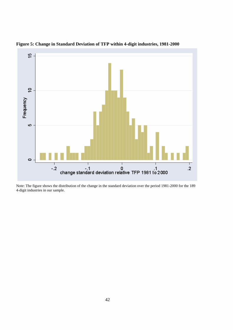
productivity distributions. Figure 5 summarises changes in productivity dispersion for all
4-digit industries in our sample, by plotting changes in the sample standard deviation of
relative TFP using a histogram. In 107 industries the standard deviation of relative TFP
declined, while in 82 industries it increased, over the period 1980-2000.
Table 2 shows the proportion of establishments that transit between quintiles of their
4-digit industry TFP distribution. The rows show the quintile at time t − 5, while the
columns show the quintile at time t. For example, the row marked quintile 5 shows that,
of the establishments that were in the bottom quintile of their industry’s TFP distribution,
five years later 22% of those that survive have moved up to the top quintile, 24% have
moved to the second quintile, 20% to the third, 21% to the fourth, and 13% remain in the
bottom quintile. This transition matrix shows that persistent cross-section dispersion is
accompanied by individual establishments changing their position within the productivity
distribution, as implied by the theoretical model.
These descriptive statistics show that there is substantial variation in growth rates, even
within industries. And that these differences in growth rates translate, in some cases, into
persistently different level of TFP. The model developed above provides one explanation for
this, and below we look at how well it describes the variation we see in the data.
3.4 The technological frontier
Before turning to the econometric evidence it is worth considering what we are capturing
in our measure of the distance to the technological frontier. We begin by using the estab-
lishment with the highest level of TFP to define the technological frontier. This approach
20

has the advantages of simplicity and of being close to the structure of the model. Another
attraction is that it potentially allows for endogenous changes in the technological frontier,
as one establishment first catches up and then overtakes the establishment with the highest
initial level of measured TFP.
For our econometric estimates, it is not important whether we correctly identify the
precise establishment with the highest level of true TFP or, more generally, whether we
correctly measure the exact position of the technological frontier. The TFP gap between
establishment i and the establishment with the highest TFP level is being used as a measure
of the potential for technology transfer. What matters for estimating the parameters of
interest is the correlation between our measure and true unobserved distance from the
technological frontier.
Year on year fluctuations in measured TFP may be due partly to measurement error
and this could lead to mis-measurement in the location of the frontier. The rich source of
information that we have on establishments in the ARD, and the series of adjustments that
we make in measuring TFP, should eliminate many of the sources of measurement error sug-
gested in the existing literature. Nonetheless, it is likely that measurement error remains.
Since we wish to abstract from high frequency fluctuations in TFP due to measurement
error, we also consider defining the technological frontier as an average of the five estab-
lishments with the highest levels of TFP relative to the geometric mean. We also report
instrumental variables estimates, estimates of the ADL(1,1) representation of the model,
and specifications where we replace our measure of distance to the frontier by a series of
dummies for the decile of the industry productivity distribution where an establishment
lies.
Finally, Table 1 shows that, on average, the log TFP gap is 0.548 which implies that on
average the frontier establishment has TFP 73% higher than non-frontier establishments
(exp(0.548) = 1.73), and that there is substantial variation in this.
21

4 Empirical results
We start by presenting evidence that our basic model of technology transfer provides a good
description of variation in the data with regards to productivity dynamics. We use these
estimates to quantify the importance of technology transfer in the growth process. We then
consider the role that foreign firms play in technology transfer.
4.1 Productivity dynamics
We start by correlating an establishment’s distance to the technological frontier in their
4-digit industry, the technology gap term, with the establishment’s TFP growth rate, con-
trolling for only year effects and industry fixed effects. This is shown in the first column of
Table 3. We see that there is a positive and significant correlation. This is close to our basic
specification in equation (8). In column 2, we add age, an indicator for whether the estab-
lishment is an affiliate of a US multinational or an affiliate of another foreign multinational,
and a term to correct for possible bias due to sample selection. The coefficient on age never
enters significiantly, while the dummy for US-owned establishments enters with a positive
and significant coefficient, indicating that the UK-based affiliates of US multinationals ex-
perience around a half of one percent faster growth than the average UK establishment. We
also include a dummy indicating whether an establishment is an affiliate of a multinational
from any other foreign country and find that this is statistically insignificant. These coef-
ficients are in line with the findings in other empirical work.22 As expected, the coefficient
on the inverse Mills ratio is positive and significant, indicating that firms that survive have,
on average, higher growth rates. In line with this, when we look at exiting firms we see that
they are mainly exiting from the lower deciles of the TFP growth distribution.
In the third column we add establishment-specific effects. These control for unobserv-
22Criscuolo and Martin (2005) provide evidence for the UK showing that the UK affiliates of US multina-tionals have a productivity advantage over UK and other foreign multinationals (located in the UK).
22
able characteristics that may be correlated with the TFP gap. We find a positive and
significant effect of the TFP gap term - other things equal, establishments further behind
the technological frontier in their 4-digit industry experience faster rates of productivity
growth than firms that are more technologically advanced. This provides evidence of tech-
nological convergence and technology transfer at the establishment-level. The magnitude
of the coefficient increases slightly when we include establishment fixed effects in column 3.
This makes sense, omitted establishment characteristics that raise the level of productivity
(e.g. good management) will be negatively correlated with the technology gap term (these
establishments will be more likely to be nearer to the technology frontier than other estab-
lishments) and so lead to negative bias in the coefficient on the technology gap. Including
establishment effects means that our model of convergence focuses on the time-series rela-
tionship between productivity in individual establishments and productivity in the frontier.
Persistent dispersion in productivity levels relates to the cross-section distribution of pro-
ductivity over different establishments. There is cross-section dispersion because different
establishments have different steady-state levels of productivity relative to the frontier, as
shaped by the fixed effects and the estimated speed of technology transfer (equation (14)).
In the fourth column we add in the growth rate of TFP in the frontier, as in the
ECM representation (equation 11). This specification allows for a more flexible long-run
relationship between frontier and non-frontier TFP. The frontier growth rate enters with a
positive and significant coefficient - establishments in industries where the frontier is growing
faster also experience faster growth. The coefficient on the gap term remains positive
and significant. This pattern of estimates is consistent with the positive cointegrating
relationship between frontier and non-frontier TFP implied by our model of technology
transfer (α2 > 0, (1− α1) > 0 and α3 = (1− α1)− α2 > 0 in equation (10)).
As mentioned above, one concern is measurement error. If we measure TFP with error
then this could induce spurious correlation, as measured TFPit−1 appears in both the right
23
and left hand sides of our regression. We address this potential problem using a number
of complementary approaches. First, we control for many sources of measurement error
in our TFP indices by using detailed micro data (as described above). Second, we include
dummies indicating which decile, in terms of distance to the frontier, the establishment is in.
Using deciles, rather than the actual distance to frontier, means that TFPit−1 does not enter
directly on the right-hand side, so measurement error can not be driving these results. These
estimates are shown in column 5 of Table 3. These show that, conditional on differences
that arise due to year and establishment effects, age and being US or other foreign-owned,
establishments in the tenth decile (those furthest away from the technological frontier),
experience 25% faster TFP growth that those very close to the frontier. The coefficients on
the decile dummies are monotonically declining, with those nearest the frontier experiencing
the slowest growth rates. We also take two further approaches - we instrument the TFP
gap term (column 2 of Table 4) and we use an alternative measure of distance from the
technological frontier based on the average of the top five establishments (column 1 of Table
4).
A final concern we deal with in Table 3, before turning to a range of other robustness
checks, is potential parameter heterogeneity. Our baseline estimation results pool across
industries, imposing common slope coefficients. We re-estimated the model separately for
each 2-digit industry.23 As shown in column 6 of Table 3, this yielded a similar pattern of
results. The median estimated coefficients, across 2-digit industries, were 0.134 for distance
from the technological frontier, 0.0006 for age, 0.013 for the US dummy and -0.01 for the
other foreign dummy. The coefficient on distance to the frontier was positive in all cases,
and in 15 out 17 2-digit industries it was significant at the 5% level. These lie close to the
baseline within groups estimates reported in column 3 of Table 3.
We now turn to a number of robustness checks. We start, in column 1 of Table 4, by
23See, for example, the discussion in Pesaran and Smith (1995).
24

considering an alternative measure of distance from the technological frontier, based on
the average TFP in the five establishments with the highest measured TFP levels.24 This
smooths the distance from the technological frontier term, and again we find a positive and
significant coefficient on the TFP gap. In column 2 we instrument relative TFP using lagged
values of the TFP gap term. We use the t-2 and t-3 lags, both of which are statistically
significant with an R-squared in the reduced form regression of 0.50, indicating that the
instruments have some power. Again, we find a similar pattern of results. The coefficient
on the gap term increases substantially (as does the standard error). This is due to the
instrumenting rather than the change in sample. A final concern about measurement error
is that TFP is measured under the assumption of perfect competition, as discussed above.
In column (3) we adjust the factor shares by an estimate of the markup (calculated at the
2-digit industry-year level). Nonetheless, the coefficient on the gap term remains positive
and significant. Finally, in column (4) we use an alternative measure of TFP growth. We
implement the Olley-Pakes technique to estimate the level of TFP and from this calculate
the growth rates and the gap. The coefficient on the gap remains positive and significant,
although the magnitude of the coefficient is somewhat reduced.
A further concern is whether we are picking up technology transfer or mean reversion.
The statistical significance of the establishment fixed effects provides evidence against re-
version to a common mean value for productivity across all establishments. There remains
the concern that each establishment may be reverting to its own mean level of productivity.
A negative realization of the stochastic shocks to technology last period, uit−1, leads to a
lower value of lagged productivity, Ait−1, and a larger value of distance from the techno-
logical frontier, AFjt−1. Reversion to the establishment’s mean level of productivity would
result in a faster rate of TFP growth, inducing a positive correlation between establishment
24This leads to a smaller sample size because we omit the frontier establishments from our estimatingsample, so in this case we are omitting the five top establishments.
25

productivity growth and lagged distance from the technological frontier. On this interpre-
tation, the identification of the parameters of interest is driven solely by variation in Ait−1.
In contrast, according to our technology transfer hypothesis, variation in the position of the
technological frontier, AFjt−1, also plays an important role.
As a robustness test, we have estimated the ADL(1,1) representation in TFP levels
from equation 10, shown in Table 5. In column (1) we find that the terms for frontier TFP
are individually and jointly statistically significant, providing evidence that our results
are not exclusively driven by variation in Ait−1. As an additional robustness test, we
estimated the equation for TFP growth in (8), but include lagged own establishment TFP
(rather than distance from the technological frontier) on the right-hand side, together with
a set of (0,1) dummies for the decile of the within-industry productivity distribution in
which the establishment was present the previous period. Even after conditioning on lagged
own establishment TFP, the decile dummies are highly statistically significant and the
coefficients on the dummies are larger for deciles further from the frontier. While they are
no longer monotonically increasing the dummies for deciles further from the frontier are
statistically different from those that are close to the frontier. In the third column we add
an additional lag of own TFP and in column (4) we instrument own lagged TFP with lags
t-2 and t-3. The results for the decile dummies hold up to these, providing further evidence
of the important role played by distance from the technological frontier.
What do these estimates imply about the economic importance of technology transfer
in growth? If we take the coefficient on the gap, multiply this by the gap for each individual
establishment, and represent this as a percentage of the establishment’s own annual growth
rate, we find that for the median establishment technology transfer accounts for 9% of total
growth (the mean is 8%). If we take it as a percentage of predicted growth (so omitting
the idiosyncratic element) we find that for the median establishment it accounts for 26% of
26

growth (the mean is 98%).25
Taken together, these estimates imply that the further a firm lags behind the techno-
logical leader the greater the potential to realize productivity growth through technology
transfer. We now turn to the question - what role is there for foreign-owned establishments
within this framework?
4.2 Foreign ownership and productivity dynamics
The existing literature emphasises the importance of foreign-owned firms in driving tech-
nology transfer, particularly in technologically less advanced countries. Productivity levels
or growth rates are typically regressed on a measure of foreign presence in an industry, such
as the share of foreign firms in employment, sales, or the total number of firms. But a
major concern about this approach is that the entry and presence of foreign-owned estab-
lishments may be endogenous to TFP growth rates, and technology transfer may occur not
only from foreign to domestic firms, but also between high performing and laggard domestic
firms. In this paper, we take an alternative approach to estimating the impact of foreign
direct investment on productivity growth of host-country firms. This allows for knowledge
spillovers from both foreign-owned multinationals and highly productive domestic firms
(including domestic multinationals, which may be sourcing technologies from abroad).
In many ways, foreign-owned establishments are just like any other. However, a large
theoretical and empirical literature finds that they are on average more productive than
domestically-owned establishments, and they may have access to superior technology from
the source country where the parent firm is based.26 Frequently, foreign-owned establish-
ments may be close to, and may advance, the technological frontier within an industry,
25 If we simply take the coefficient on the gap and multiply it by the average gap, we obtain a much largerestimate of the contribution of technology transfer. This is driven by the influence of outlying observationsthat affect mean productivity growth and levels.26For empirical evidence on the higher productivity of foreign-owned establishments and multinationals
more generally, see Criscuolo and Martin (2003), Doms and Jensen (1998) and Griffith (1999). This evidenceis consistent with there being fixed costs to becoming a multinational firm, as formalized in Helpman et al.(2004) and Markusen (2002).
27
thereby providing a source of knowledge spillovers for domestically-owned establishments.
In the UK, the majority of foreign investment has come from the US, and many papers have
documented the fact that the US is the technological leader in a large number of industries.
In addition, Criscuolo and Martin (2005) show that it is specifically US multinationals op-
erating within the UK that have a productivity advantage over UK multinationals. The
positive and sometimes significant dummy on US-owned establishments in Tables 3, 4 and
5 suggests that this is also the case in our sample. We also include a dummy to control for
foreign affiliates of all other nationalities, but this is never significant. Therefore, in this
section we focus our attention on the impact that US multinationals have on productivity
growth.
In our model, US-owned establishments influence the productivity growth of non-frontier
establishments in so far as they advance the technological frontier. Table 6 quantifies this
impact. We first show the extent to which US affiliates are present in the UK. Column
1 shows that, using data on the population of plants, US affiliates account for around
9% of employment, ranging from 30% in the high-tech office machinery and computer
equipment sector, to zero in the leather and leather goods sector. Column 2 shows that
US affiliates were the frontier establishment around 13% of the time across industries over
the period 1980-2000. There is again a large range, from US affiliates being at the frontier
around a quarter of the time in non-metallic mineral products to only three percent of
the time in textiles. As we would expect, the presence of US-owned establishments in
an industry is positively correlated with the likelihood that they are at the technological
frontier. US-owned establishments have the highest presence in high-tech industries such
as office machinery and computer equipment, chemicals and instrument engineering, and
make up the technological frontier over 25% of the time in these sectors.
The third column shows how far foreign-owned establishments advance the technolog-
ical frontier, where they are the technological leader. Using our relative TFP measure we
28

calculate the productivity gap between the US-owned frontier and the most technologically
advanced non—US-owned establishment. When the frontier is a non—US-owned establish-
ment this figure is zero. This distance averages two percent across all manufacturing indus-
tries, and ranges from zero to 5 percent. Looking just at cases where a US affiliate is the
frontier, on average it advances it by 19%. To examine how important US establishments
are in facilitating technology transfer to non-frontier UK-based establishments, we calculate
the proportion of technology transfer (δ1TFPGAPit−1) due to US affiliates advancing the
frontier (δ1³TFPGAPit−1 − TFPGAP ∗nfit−1
´), where TFPGAP ∗nfit−1 is a measure of what
the TFP gap would have been if no US establishments had been present to advance the
frontier, holding all else equal. This is equal to
δ1
³TFPGAPit−1 − TFPGAP ∗nfit−1
´δ1TFPGAPit−1
= 1−TFPGAP ∗nfit−1TFPGAPit−1
.
We calculate this for each individual establishment and take the mean over all establish-
ments. This is shown in column 4 of Table 6. We see that this ranges from zero, in industries
where no US affiliates are present at the frontier, to 20% in mechanical engineering. The
pattern across industries suggests that US affiliates make a larger contribution to technology
transfer in high-technology industries such as mechanical engineering, instruments, office
machinery and data processing equipment and chemicals.
5 Conclusions
The recent literature has emphasised deregulation and the opening up of markets as a
key source of productivity growth. One important mechanism through which this works
is technology transfer, both from domestic leaders and from inward investment from more
technologically advanced economies. But the importance of technology transfer raises the
puzzle of how this can be reconciled with persistent dispersion in productivity levels across
establishments within narrowly defined industries.
29

In this paper we developed a model of technology transfer in which persistent dispersion
is an equilibrium outcome. We estimated a structural model of technological convergence at
the micro level, that included the technological distance between an establishment and the
frontier as a measure of the potential for technology transfer. We found statistically signif-
icant and quantitatively important evidence of catch-up to the technological leader. Other
things equal, establishments further behind the technological frontier experience faster rates
of productivity growth. We looked specifically at the role of the affiliates of US multination-
als in contributing to productivity growth by raising the potential for technology transfer.
The existing literature on the links between foreign presence and productivity growth has
not included measures of distance from the technological frontier that we find to be impor-
tant here. Our findings suggest that US-affiliates make a positive contribution to technology
transfer in the UK, and that this is larger in high-technology industries, consistent with pri-
ors about US technological advantage.
30

Figure 1: Unchanged Technological Leadership
31

Figure 2: Endogenous Change in Technological Leadership
32

References
[1] Acemoglu, D, Aghion, P and Zilibotti, F (2002) "Distance to Frontier, Selection, and
Economic Growth", NBER Working Paper, #9066.
[2] Aghion, P and Howitt, P (1997) Endogenous Growth Theory, MIT Press.
[3] Aitken, B and A Harrison (1999) ’Do domestic firms benefit from direct foreign in-
vestment? Evidence from Venezuela’ American Economic Review (June 1999) 605 -
618
[4] Baily, N, Hulten, C and Campbell, D (1992) "Productivity Dynamics in Manufacturing
Plants", Brookings Papers on Economic Activity, Microeconomics, 187-267.
[5] Baily, M and Chakrabarty, A (1985) "Innovation and Productivity in US Industry",
Brookings Papers on Economic Activity, 2, 609-32.
[6] Barro, R and Sala-i-Martin, X (1995) Economic Growth, McGraw Hill: New York.
[7] Bartelsman, Eric and Mark Doms, (2000) "Understanding Productivity: Lessons from
Longitudinal Microdata", Journal of Economic Literature, XXXVIII, 569-94.
[8] Bernard, A and Durlauf, S (1996) "Interpreting Tests of the Convergence Hypothesis",
Journal of Econometrics, 71(1-2), 161-73.
[9] Bernard, A and Jensen, J (1995) "Exporters, Jobs, and Wages in US Manufacturing:
1976-87", Brookings Papers on Economic Activity: Microeconomics, 67-112.
[10] Bernard, A and Jones, C (1996) "Comparing apples to oranges: productivity conver-
gence and measurement across industries and countries", American Economic Review,
1,216-38.
[11] Blomstrom (1989) Foreign Investment and Spillovers Routledge: London
33

[12] Cameron, G., Proudman, J. and Redding S., (1998), "Productivity Convergence and
International Openness" Chapter 6 in Proudman J. and Redding S. (eds), Openness
and Growth, Bank of England: London
[13] Caves D., Christensen L., and Diewert E., (1982a) "The Economic Theory of Index
Numbers and the Measurement of Input, Output and Productivity", Econometrica,
50, 6, 1393-1414.
[14] Caves D., Christensen L., and Diewert E., (1982b) "Multilateral Comparisons of Out-
put, Input and Productivity Using Superlative Index Numbers", Economic Journal,
92, 73-86.
[15] Criscuolo and Martin (2005) "Multinationals, and US productivity leadership: Evi-
dence from Britain", AIM Working Paper, United Kingdom.
[16] Cohen, W.M., (1995) "Empirical Studies of Innovative Activity ," in P. Stoneman,
ed., Handbook of the Economics of Innovation and Technical Change, Basil Blackwell:
Oxford, 1995.
[17] Davis, Steven J and John C. Haltiwanger. (1991) "Wage Dispersion between and within
U.S. Manufacturing Plants, 1963-86", Brookings Papers on Economic Activity, Micro-
economics, 115-80.
[18] Davis, Steven J, Haltiwanger, John C. and Scott Schuh (1996) Job Creation and De-
struction, MIT Press.
[19] Disney, R., Haskel, J., and Heden, Y. (2003) "Restructuring and Productivity Growth
in UK Manufacturing", Economic Journal, 113(489), 666-694.
[20] Djankov, S, La Porta, R, Lopez-de-Silanes, F and Shleifer, A (2002) "The Regulation
of Entry", Quarterly Journal of Economics, CXVII, 1-37.
34

[21] Doms, M and Jensen, J. Bradford (1998) "Comparing Wages, Skills, and Productivity
Between Domestically and Foreign-owned Manufacturing Establishments in the United
States", in Baldwin, R et al. (eds), Geography and Ownership as Bases for Economic
Accounting, University of Chicago Press, 235-58.
[22] Dunne, T., Roberts M. J., and Samuelson L., (1989) "The Growth and Failure of U.S.
Manufacturing Plants", Quarterly Journal of Economics, 104(4):671-98..
[23] Eeckhout, J and Jovanovic, B (2002) "Knowledge Spillovers and Inequality", American
Economic Review, 92(5), 1290-1307.
[24] Ericson, R and Pakes, A (1995) "Markov-Perfect Industry Dynamics: A Framework
for Empirical Work", Review of Economic Studies, 62, 53-82.
[25] Foster, L, Haltiwanger, J and Krizan, C (2002) "The Link Between Aggregate and
Micro Productivity Growth: Evidence from Retail Trade", NBER Working Paper,
#9120.
[26] Geroski, P, Machin, S and Van Reenen, J (1993) "The Profitability of Innovating
Firms", RAND Journal of Economics, 24(2), 198-211.
[27] Girma, S. and Wakelin, K. (2000) ‘Are There Regional Spillovers from FDI in the
UK?’, GEP research paper, 2000/16, University of Nottingham.
[28] Globerman (1979) “Foreign direct investment and spillover efficiency benefits in Cana-
dian manufacturing industries” Canadian Journal of Economics, 12: 42-56.
[29] Görg, H and Greenaway, D (2002) ‘Much Ado About Nothing? Do Domestic Firms
Really Benefit from Foreign Direct Investment?’, CEPR Discussion Paper, 3485.
[30] Görg, H. and Strobl, E. (2001) ‘Multinational Companies and Indigenous Development:
An Empirical Analysis’, European Economic Review, 46(7), 1305-22.
35

[31] Griffith, R (1999) "Using the ARD Establishment-level Data to Look at Foreign Own-
ership and Productivity in the United Kingdom", Economic Journal, 109, F416-F442.
[32] Griffith, R, Redding, S and Van Reenen, J (2003) "R&D and Absorptive Capacity:
Theory and Empirical Evidence", Scandinavian Journal of Economics, 105(1), 99-118.
[33] Griffith, R, Redding, S and Van Reenen, J (2004) "Mapping the Two Faces of R&D:
Productivity Growth in a Panel of OECD Industries", Review of Economics and Sta-
tistics, forthcoming.
[34] Griliches, Z (1992) "The search for R&D Spillovers", The Scandinavian Journal of
Economics, 94, 29-47.
[35] Griliches, Z. and Lichtenberg, F. (1984), "R&D and Productivity Growth at the In-
dustry Level: Is There Still a Relationship?" in (ed) Griliches, Z. R&D, Patents and
Productivity, NBER and Chicago University Press.
[36] Grossman, G and Helpman, E (1991) Innovation and Growth in the Global Economy,
MIT Press: Cambridge MA.
[37] Hall, R (1988) "The Relationship Between Price and Marginal Cost in US Industry",
Journal of Political Economy, 96 (5), 921-947
[38] Harrigan (1997), "Technology, Factor Supplies and International Specialisation",
American Economic Review, 87, 475-94.
[39] Harris, R and Robinson, C (2004) "Spillovers from foreign ownership in the United
Kingdom: estimates for UK manufacturing using the ARD", National Institute Eco-
nomic Review, 187, January.
[40] Haskel, J., Pereira, S., and Slaughter, M. (2002) ‘Does Inward Foreign Direct Invest-
ment Boost the Productivity of Domestic Firms?’, CEPR Discussion Paper, 3384.
36

[41] Heckman, J (1976) "The Common Structure of Statistical Models of Truncation, Sam-
ple Selection, and Limited Dependent Variables and a Simple Estimator for Such Mod-
els", Annals of Economic and Social Measurement, 5, 475-92.
[42] Hendry, D (1996) Dynamic Econometrics, Oxford University Press: Oxford.
[43] Helpman, E, Melitz, M, and Yeaple, S (2004) "Export Versus FDI With Heterogeneous
Firms", American Economic Review, 300-16.
[44] Hopenhayn, Hugo. (1992) "Entry, Exit, and Firm Dynamics in Long Run Equilibrium",
Econometrica, 60(5), 1127-1150.
[45] Howitt, P (2000) ‘Endogenous Growth and Cross-country Income Differences’, Amer-
ican Economic Review, 90(4), 829-46.
[46] Jovanovic, Boyan. (1982) "Selection and the Evolution of Industry", Econometrica,
vol. 50, no. 3, May, 649-70.
[47] Keller, W (2004) "International Technology Diffusion", Journal of Economic Litera-
ture, forthcoming.
[48] Keller, W and Yeaple, S (2003) ‘Multinational Enterprises, International Trade, and
Productivity Growth: Firm-level Evidence from the United States’, NBER Working
Paper, #9504.
[49] Klette, T and Z. Griliches (1996) "The inconsistency of common scale estimators when
output prices are unobserved and endogenous" Journal of Applied Econometrics, 11
(4), 343-361
[50] Levinsohn, J and Petrin, A (2003) "Estimating Production Functions using Inputs to
Control for Unobservables", Review of Economic Studies, 70, 317-41.
37

[51] Markusen, J (2002) Multinational Firms and the Theory of International Trade, MIT
Press: Cambridge.
[52] Melitz, Marc J. (2003) "The Impact of Trade on Intra-Industry Reallocations and
Aggregate Industry Productivity", Econometrica, Vol. 71, November 2003, pp. 1695-
1725.
[53] Nicoletti, G and Scarpetta, S (2003) "Regulation, Productivity and Growth: OECD
Evidence", OECD Economics Department Working Paper, 347.
[54] Olley, Steve and Ariel Pakes (1996) "The dynamics of Productivity in the Telecommu-
nications equipment industry" Econometrica 64 (6), pp 1263-1297
[55] Parente, S and Prescott, E (1994) "Barriers to Technology Adoption and Develop-
ment", Journal of Political Economy, 102(2), 298-321.
[56] Parente, S and Prescott, E (1999) "Monopoly Rights: A Barrier to Riches", American
Economic Review, 89(5), 1216-33.
[57] Pavnick, Nina (2002) "Trade Liberalization, Exit, and Productivity Improvements;
Evidence form Chilean Plants" Review of Economic Studies, 69, 245-276
[58] Pesaran, H. and Smith, R. (1995), "Estimating Long Run Relationships from Dynamic
Heterogeneous Panels", Journal of Econometrics, 68, 79-113.
[59] Roeger, W. (1995) "Can Imperfect Competition Explain the Difference Between Pri-
mal and Dual Productivity Measures? Estimates for US Manufacturing", Journal of
Political Economy, 103(2), 316-30.
[60] Romer, P (1990) "Endogenous Technological Change", Journal of Political Economy,
98(5), S71-102.
38

[61] Smarzynska Javorcik, B (2004) “Does Foreign Direct Investment Increase the Pro-
ductivity of Domestic Firms? In Search of Spillovers through Backward Linkages”,
American Economic Review, forthcoming.
[62] Teece, D (1977) "Technology transfer by multinational firms: the resource cost of
transferring technological know-how", Economic Journal, 87 (346), 242-261.
39

40
Table 1: Descriptive Statistics Variable Mean Standard deviation
ijtTFP∆ 0.003 0.129
1−ijtTFPGAP 0.548 0.317
FjtTFP∆ 0.003 0.303Age 8.127 5.122US dummy 0.120 0.325Other foreign dummy 0.105 0.306Note: The sample includes 103,664 observations on all non-frontier establishments over the period 1980-2000. Means are weighted by the inverse of the sampling probability and employment. Figure 3: Evolution of TFP in the office machinery and computer equipment industry
Note: The figure shows the distribution of TFP in 2-digit industry no.33 over time. TFP in each establishment is measured relative to the geometric mean of all other establishments in the same 4-digit industry (averaged over all years). The sample includes 627 observations on non-frontier establishments over the period 1981-2000. The horizontal bar shows the median, the top and bottom of the horizontal lines represent the 95th and 5th percentile respectively.

41
Figure 4: Evolution of TFP in the footwear and clothing industry
Note: The figure shows the distribution of TFP in 2-digit industry 45 over time. TFP in each establishment is measured relative to the geometric mean of all other establishments in the same 4-digit industry (averaged over all years). The sample includes 6129 observations on non-frontier establishments over the period 1981-2000. The horizontal bar shows the median, the top and bottom of the horizontal lines represent the 95th and 5th percentile respectively.
42
Figure 5: Change in Standard Deviation of TFP within 4-digit industries, 1981-2000
Note: The figure shows the distribution of the change in the standard deviation over the period 1981-2000 for the 189 4-digit industries in our sample.

43
Table 2: Transition matrix Quintile of TFP distribution t Quintile of TFP distribution, t-5
1 2 3 4 5 Total
1 37.71 29.39 18.27 9.41 5.22 100 2 26.46 28.06 25.16 13.76 6.57 100 3 17.39 26.48 25.13 22.08 8.92 100 4 18.03 20.22 28.58 21.92 11.25 100 5 22.19 23.81 19.81 21.47 12.73 100 Total 24.75 25.88 23.36 17.35 8.67 100 Note: The table shows the proportion of establishments by quintile of the TFP distribution within their 4-digit industry in period t-5 and t, averaged over the four five year periods in our sample. The quintiles are defined across all establishments in our sample (including entrants and exitors), while only establishments that are present in both period t-5 and t are included in the table. The figures are weighted by the inverse of the sampling probability and employment.

44
Table 3: Catch-up model dep var: ijtTFP∆ (1) (2) (3) (4) (5) (6)
Obs 103,664 103,664 103,664 103,664 103,664 103,664
FjtTFP∆ 0.111
(0.012)
1−ijtTFPGAP 0.091 0.091 0.117 0.199 0.134 (0.012) (0.012) (0.015) (0.022) Age 0.0002 0.0003 0.0002 0.001 0.0006 (0.0005) (0.0006) (0.0006) (0.0004) US dummy 0.005 0.007 0.010 0.007 0.013 (0.002) (0.005) (0.005) (0.006) Other foreign -0.009 -0.020 -0.020 -0.022 -0.010 (0.006) (0.014) (0.014) (0.015) DD2 0.062 (0.006) DD3 0.098 (0.008) DD4 0.123 (0.008) DD5 0.146 (0.010) DD6 0.164 (0.009) DD7 0.188 (0.011) DD8 0.224 (0.013) DD9 0.251 (0.013) DD10 0.254 (0.017) Inverse mills ratio 0.006 0.043 0.038 0.021 0.032 (0.004) (0.010) (0.011) (0.012) Year dummies Yes Yes Yes Yes Yes Yes 4-digit industry dummies
Yes Yes - - - -
Within groups No No Yes Yes Yes Yes Note: Regressions are estimated on all non-frontier establishments for 1980-2000. All columns are weighted by the inverse of the sampling probability and employment. Standard errors in brackets are clustered at the 4-digit industry.
FjtTFP∆ is tfp growth in the frontier. 1−ijtTFPGAP is tfp relative to frontier in the previous period. DD* are dummies
representing the decile of the within 4-digit industry year distribution of 1−ijtTFPGAP where DD10 is the decile for establishments with the largest gap with the frontier. DD1 the decile for those closest to the frontier is omitted. Column (6) reports the median of the coefficients from 2-digit industry level regressions.
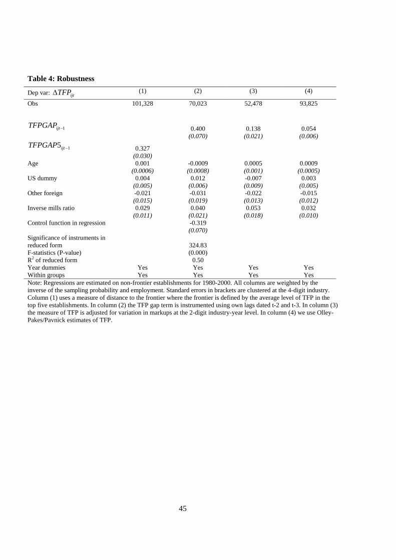
45
Table 4: Robustness
Dep var: ijtTFP∆ (1) (2) (3) (4)
Obs 101,328 70,023 52,478 93,825
1−ijtTFPGAP 0.400 0.138 0.054 (0.070) (0.021) (0.006)
15 −ijtTFPGAP 0.327
(0.030) Age 0.001 -0.0009 0.0005 0.0009 (0.0006) (0.0008) (0.001) (0.0005) US dummy 0.004 0.012 -0.007 0.003 (0.005) (0.006) (0.009) (0.005) Other foreign -0.021 -0.031 -0.022 -0.015 (0.015) (0.019) (0.013) (0.012) Inverse mills ratio 0.029 0.040 0.053 0.032 (0.011) (0.021) (0.018) (0.010) Control function in regression -0.319 (0.070) Significance of instruments in reduced form F-statistics (P-value)
324.83 (0.000)
R2 of reduced form 0.50 Year dummies Yes Yes Yes Yes Within groups Yes Yes Yes Yes Note: Regressions are estimated on non-frontier establishments for 1980-2000. All columns are weighted by the inverse of the sampling probability and employment. Standard errors in brackets are clustered at the 4-digit industry. Column (1) uses a measure of distance to the frontier where the frontier is defined by the average level of TFP in the top five establishments. In column (2) the TFP gap term is instrumented using own lags dated t-2 and t-3. In column (3) the measure of TFP is adjusted for variation in markups at the 2-digit industry-year level. In column (4) we use Olley-Pakes/Pavnick estimates of TFP.

46
Table 5: ADL(1,1) and ECM specifications (1) (2) (3) (4) Dependent variable
ijtTFP ijtTFP∆ ijtTFP∆ ijtTFP∆ Obs 103,664 103,664 84,232 70,023 TFPijt-1 0.545 -0.342 -0.375 -0.271 (0.036) (0.051) (0.034) (0.035) TFPijt-2 0.068 (0.016) TFPFjt 0.044 (0.009) TFPFjt-1 0.021 (0.008) Age 0.0012 0.001 0.0005 -0.0004 (0.0005) (0.0005) (0.0006) (0.0008) US dummy 0.006 0.006 0.010 0.010 (0.005) (0.005) (0.006) (0.008) Other foreign dummy -0.019 -0.021 -0.024 -0.025 (0.017) (0.016) (0.019) (0.020) DD2 0.025 0.026 0.024 (0.005) (0.007) (0.007) DD3 0.039 0.042 0.041 (0.009) (0.009) (0.009) DD4 0.048 0.050 0.047 (0.010) (0.010) (0.010) DD5 0.058 0.060 0.057 (0.010) (0.010) (0.010) DD6 0.062 0.064 0.060 (0.013) (0.011) (0.010) DD7 0.068 0.069 0.065 (0.015) (0.013) (0.013) DD8 0.085 0.085 0.082 (0.017) (0.014) (0.013) DD9 0.087 0.093 0.089 (0.021) (0.016) (0.017) DD10 0.079 0.079 0.075 (0.023) (0.019) (0.020) Inverse mils ratio 0.006 0.006 -0.006 -0.005 (0.015) (0.014) (0.026) (0.030) Control function in regression -0.116 (0.032) Significance of instruments in reduced form F-statistics (P-value)
10867.83 (0.000)
R2 of reduced form 0.69 Year dummies Yes Yes Yes Yes Within groups Yes Yes Yes Yes Notes: Regressions are estimated on non-frontier establishments for 1980-2000. All columns are weighted by the inverse of the sampling probability and employment. Standard errors in brackets are clustered at the 4-digit industry. In column 1 frontier TFP (TFPFt) and lagged frontier TFP (TFPFt-1) are jointly significant. Dependent variable in columns 2 to 4 is TFP growth. In column 3 we add in TFP t-2 and in column 4 we instrument TFP t-1 with TFP t-2 and TFP t-3.

47
Table 6: The contribution of affiliates of US multinationals, 1980-2000
US affiliates: Sector Share of
industry employment %
% of time frontier
Advancement of the frontier
Advancement of the frontier
as a proportion of the total gap
22 metal manufacturing 5 17 0.02 0.0724 non-metallic mineral products 4 24 0.04 0.1525 + 26 chemicals and man-made fibres
18 23 0.05 0.14
31 metal goods n.e.s. 8 6 0.01 0.0832 mechanical engineering 15 18 0.04 0.2033 office machinery and data processing equipment
30 13 0.03 0.15
34 electrical and electronic engineering
10 10 0.01 0.06
35 motor vehicles and parts 16 17 0.05 0.1036 other transport equipment 3 4 0.00 0.0037 instrument engineering 20 22 0.02 0.1341 + 42 food, drink and tobacco 6 14 0.02 0.0643 textiles 4 3 0.01 0.0244 leather and leather goods 0 0 0 045 footwear and clothing 2 4 0.01 0.0347 paper, paper products and publishing
8 9 0.02 0.12
48 rubber and plastics 8 21 0.03 0.1349 + 46 other manufacturing, timber
4 1 0.00 0.01
All manufacturing 9 13 0.02 0.10Notes: All means are weighted by the inverse of the sampling probability and employment. Column (1) shows the annual average proportion of employment in each 4-digit industry with the 2-digit industry that is in affiliates of US firms, 1980-2000. Column (2) shows the percentage of times an affiliate of a US firm is the most productive establishment in its 4-digit industry. Column (3) shows how far the US affiliate advances the frontier (i.e. the distance between the US affiliate and the nearest non-US-owned establishment) when it is the frontier. This is the mean of ln(AF US/ AF Non-US). Column 4 shows the amount that affiliates of US firms advance the frontier (increase the TFP gap) divided by the total gap, calculated at the establishment level and averaged.