The Costs of Agglomeration: House and Land Prices in French Cities
Pierre-Philippe Combes∗†
University of Lyon and Sciences Po
Gilles Duranton∗‡
University of Pennsylvania
Laurent Gobillon∗§
Paris School of Economics
Revised: January 2018
Abstract: We develop a new methodology to estimate the elasticityof urban costs with respect to city population using French house andland price data. After handling a number of estimation concerns, wefind that the elasticity of urban cost increases with city population withan estimate of about 0.03 for an urban area with 100,000 inhabitants to0.08 for an urban area of the size of Paris. Our approach also yieldsa number of intermediate outputs of independent interest such as theshare of housing in expenditure, the elasticity of unit house and landprices with respect to city population, and distance gradients for houseand land prices.
Key words: urban costs, house prices, land prices, land use, agglomeration
jel classification: r14, r21, r31
∗We thank four anonymous referees, the editor Stéphane Bonhomme, conference and seminar participants, MonicaAndini, Fabien Candau, Morris Davis, Jan Eeckhout, Sanghoon Lee, François Ortalo-Magné, Gilles Orzoni, HenryOverman, Jean-Marc Robin, Stuart Rosenthal, Nathan Schiff, Daniel Sturm, and Yuichiro Yoshida for their commentsand suggestions. We also thank Pierre-Henri Bono, Julian Gille, Giordano Mion, and Benjamin Vignolles for theirhelp with the data. Finally, we are grateful to the Service de l’Observation et des Statistiques (SOeS) - Ministère del’Écologie, du Développement durable et de l’Énergie for giving us on-site access to the data and to the casd (Centre d’accèssécurisé aux données founded by the French National Research Agency (anr), “Investissements d’Avenir” programANR-10-EQPX-17) for remote access to the French Family Expenditure Survey.
†University of Lyon, cnrs, gate-lse umr 5824, 93 Chemin des Mouilles, 69131 Ecully, France and Sciences Po,Economics Department, 28, Rue des Saints-Pères, 75007 Paris, France (e-mail: [email protected]; website: https://www.gate.cnrs.fr/ppcombes/). Also affiliated with the Centre for Economic Policy Research.
‡Wharton School, University of Pennsylvania, 3620 Locust Walk, Philadelphia, pa 19104, usa (e-mail: duran-
[email protected]; website: https://real-estate.wharton.upenn.edu/profile/21470/). Also affiliated withthe Centre for Economic Policy Research and the National Bureau of Economic Research.
§pse-cnrs, 48 Boulevard Jourdan, 75014 Paris, France (e-mail: [email protected]; website: http://
laurent.gobillon.free.fr/). Also affiliated with the Centre for Economic Policy Research and the Institute for theStudy of Labor (iza).

1. Introduction
As a city’s population grows, three major changes potentially occur. First, larger cities are expected
to be more productive as agglomeration effects become stronger. Second, larger cities are expected
to become more expensive as the cost of housing and urban transport rises. The price of other
goods may also be affected. Third, larger cities may differ in how attractive they are in terms
of amenities. From past research, we know a fair amount about agglomeration, we have some
knowledge about urban amenities but we know virtually nothing about urban costs and how they
vary with city population. Although high housing prices and traffic jams in Central Paris, London,
or Manhattan are for everyone to observe, we know of no systematic evidence about urban costs
and their magnitude. This paper seeks to fill that gap.
To that end, we develop a new methodology to estimate the elasticity of urban costs with respect
to city population using French data about house and land prices and household expenditure. Our
baseline estimates range from about 0.03 for an urban area with 100,000 inhabitants to 0.08 for an
urban area of the size of Paris. Put differently, a 10% larger population in a small city leads to a
0.3% increase in expenditure for its residents to remain equally well off. For a city with the same
population as Paris, the same 10% increase in population implies a 0.8% increase in expenditure.
These figures are ‘all else constant’, including the urban area of cities. Allowing cities to increase
their physical footprint as they grow in population reduces the magnitude of the elasticity of urban
costs by sa factor of about two. In the ‘short run’, we estimate instead larger elasticities in the 0.1-0.3
range as housing supply does not fully adjust to population increases. Our approach also yields
a number of intermediate outputs of independent interest such as distance gradients for land and
house prices, the share of housing in expenditure, and the elasticities of land and house prices with
respect to city population.
Plausible estimates for urban costs are important for a number of reasons. In many countries,
urban policies attempt to limit the growth of cities. These restrictive policies, which often take the
form of barriers to labour mobility and stringent land use regulations that limit new constructions,
are particularly prevalent in developing countries (see Desmet and Henderson, 2015, for a review).
The underlying rationale for these policies is that the population growth of cities imposes large
costs to already established residents by bidding up housing prices and crowding out the roads.
Our analysis shows that in the French case, the costs of having larger cities are modest for most
1

cities and of about the same magnitude as agglomeration economies. This lends little support to
the imposition of barriers to urban growth. Quite the opposite, urban costs increase much faster
when cities are prevented from adjusting their supply of housing.
More generally, households allocate a considerable share of their resources to housing and
transport. In France, homeowners and renters in the private sector devote on average 33.4% of
their expenditure to housing and 13.5% to transport.1 As we document below, there are sizeable
differences across cities in how much households spend on housing as its cost varies greatly across
places. Understanding this variation is thus a first-order allocation issue.
Urban costs also matter for how we think about cities in theory. Following Henderson (1974)
and Fujita and Ogawa (1982), cities are predominantly viewed as the outcome of a tradeoff between
agglomeration economies and urban costs. Much of contemporary urban theory relies or builds
on this tradeoff. Fujita and Thisse (2002) dub it the ‘fundamental tradeoff of spatial economics’.
The existence of agglomeration economies is now well established and much has been learnt about
their magnitude.2 To assess the fundamental tradeoff of spatial economics empirically, evidence
about urban costs is obviously needed.
To measure how urban costs vary with city population, three challenges must be met. The
first regards the definition and measurement of urban costs since they can take a variety of forms.
Using a simple consumer theory approach, we define the elasticity of urban costs with respect to
city population as the percentage increase in expenditure that residents in a city must incur when
population grows by one percent, keeping utility constant. At a simple spatial equilibrium, this
elasticity is equal to the product of the share of housing in expenditure and the elasticity of housing
prices with respect to city population, both taken at the city centre.3 We also show that the elasticity
of housing prices can be decomposed into the product of the share of land in housing construction
and the population elasticity of land prices.
1Our figure of 33.4% for housing is the mean between the figure for renters and the figure for homeowners for2006-2011 in the French expenditure survey. It is higher than the aggregate share of housing in expenditure of 27%reported by cgdd (2015) because we exclude rural areas where housing is less expensive and renters living in publichousing who often pay well below market price. The figure for transport is from 2010 and covers the entire country(cgdd, 2015). In the us, households devote 32.8% of their expenditure to housing and 17.5% to transport (us bts, 2013).In both countries, transport is defined as all forms of personal transport but most of it is road transport. Air transportrepresents only 6% of transport expenditure in France and 5% in the us.
2See Puga (2010) and Combes and Gobillon (2015) for reviews. See also Combes, Duranton, and Gobillon (2008),Combes, Duranton, Gobillon, and Roux (2010), or Combes, Duranton, Gobillon, Puga, and Roux (2012) for some workon French cities.
3At the equilibrium, for locations closer to the centre higher housing costs offset lower transport costs. Then, wework with prices at the centre because we can, to a first approximation, ignore travel costs for these locations.
2

After this conceptual clarification, our second challenge is to gather data to implement our
approach empirically. For housing prices, we rely on detailed price indices that are estimated
for French municipalities between 2000 and 2012. For land prices, we exploit a unique record
of transactions for land parcels with a development permit from 2006 to 2012. For housing
expenditure we use a household expenditure survey. For the share of land in housing, we rely
on the results obtained in our companion paper (Combes, Duranton, and Gobillon, 2016) which
provides a detailed investigation of the production function for housing. Finally, we gathered a
vast array of data at the level of municipalities and urban areas.
Our third challenge is the actual estimation of our key elasticities and shares. For the elasticity of
both housing and land prices at the centre with respect to city population, we first need to estimate
housing and land prices at the centre of each city. This first exercise poses one main difficulty,
estimating an appropriate distance gradient for each city. We show that our results are robust
to how we handle the distribution of heterogenous residents within cities and to our choices of
functional form, specification, and city centres.
Next, when regressing housing and land prices at the centre on city population, our main worry
is the endogeneity of city population. We employ a variety of approaches to assess the robustness
of our baseline results, including extensive control variables at both the municipality and city
level and instrumental variables. We also show that house and land prices both imply similar
estimates for the elasticity of urban costs. Finally, we also address a number of related endogeneity
concerns regarding the estimation of the share of housing in expenditure and how it varies with
city population.
Tolley, Graves, and Gardner (1979), Thomas (1980), Richardson (1987), Henderson (2002), and
Au and Henderson (2006) are the main antecedents to our research on urban costs.4 To the best
of our knowledge, this short list is close to exhaustive. Despite the merits of these works, none of
their estimates has had much influence. We attribute this lack of credible estimate for urban costs
and the scarcity of research on the subject to a lack of integrated framework to guide empirical
work, a lack of appropriate data, and a lack of attention to a number of identification issues — the
4Thomas (1980) compares the cost of living for four regions in Peru focusing only on the price of consumptiongoods. Richardson (1987) compares ‘urban’ and ‘rural’ areas in four developing countries. Closer to the spirit of ourwork, Henderson (2002) regresses commuting times and rents to income ratio for a cross-section of cities in developingcountries. Like us, Au and Henderson (2006) are interested in the tradeoff between agglomeration benefits and urbancosts. They use nonetheless a very different approach and investigate the net productivity gains associated with citysize instead of trying to separate the costs from the benefits of cities.
3

three main innovations of this paper.
The elasticity of housing prices with respect to city population is also estimated by Albouy
(2008), Bleakley and Lin (2012), and Baum-Snow and Pavan (2012). These papers estimate one of
the quantities we are interested in here but do so with very different objectives in mind. They also
ignore the location of properties within their metropolitan area, a first-order empirical issue as we
show below. There is also a literature that measures land values for a broad cross-section of urban
(and sometimes rural) areas (Davis and Heathcote, 2007, Davis and Palumbo, 2008, Albouy and
Ehrlich, 2012). We enrich it by considering the internal geography of cities and by investigating
the determinants of land prices, population in particular, at the city level.
2. Model
We want to estimate how the cost of living in cities increases with their population. To provide a
rigourous definition of urban costs and some guidance about how to estimate them empirically,
we consider a model where households choose in which city to live and work, where to reside in
this city, and how much housing and other goods to consume at their chosen location.
The utility of a resident at location ` in city c with population Nc is given by U(h(`),x(`),Mc)
where Mc denotes the quality of amenities in the city, h(`) is housing consumption, and x(`) is
the consumption of a composite good. Utility is increasing in all its arguments and is strictly
quasi-concave. The budget constraint is,
Wc ≥ P(`) h(`) + τ(`) + Qc x(`) , (1)
where Wc is the wage that prevails in city c, P(`) is the price of housing at location `, τ(`) is the
cost of transport at the same location, and Qc is the city price of the composite consumption good.5
We can solve the consumer problem in steps. First, households choose a city. Then, they
choose a residential location ` in their city. Finally, residents maximise their utility with respect
to their consumption of housing h(`) and their consumption of the composite good x(`) subject
to the budget constraint (1). We start with this last step and consider its dual. Omitting the city
subscript c, we note the expenditure function for a resident at location ` as E(P(`),τ(`),Q, M, U) =
5A special case of our model is the monocentric model of Alonso (1964), Mills (1967), and Muth (1969). In this model,` measures the distance to the central business district (cbd) where all the jobs are located. Residents must commute tothis cbd at a cost τ(`) = τ × `. The results that follow do not rely on these restrictions.
4
P(`) h(`) + τ(`) + Q x(`). This function describes the minimum total expenditure on housing,
transport, and the composite consumption good needed at location ` to achieve utility U.
We can now examine the effect of a marginal increase in city population on the resident located
at location `. Totally differentiating the expenditure function with respect to population leads to,
dE(P(`),τ(`),Q,M, U)
dN=
∂E(P(`),τ(`),Q,M, U)
∂P(`)dP(`)
dN+
dτ(`)
dN
+∂E(P(`),τ(`),Q,M, U)
∂QdQdN
+∂E(P(`),τ(`),Q,M, U)
∂MdMdN
. (2)
This equation indicates that, for a given location `, the change in expenditure that is needed to keep
utility constant following a change in city population works through four channels: the change in
expenditure that arises from the change in housing prices at location `, the change in transport cost
at location ` (e.g., more congestion), the change in expenditure due to the change in the price of
the composite good, and the change in expenditure associated with the change in amenities.
Applying Shephard’s lemma to equation (2) and omitting the arguments of the expenditure
function to ease notations, we obtain,
dEdN
= h(P(`),Q,U)dP(`)
dN+
dτ(`)
dN+ x(P(`),Q,U)
dQdN
+∂E∂M
dMdN
, (3)
where h(P(`),Q,U) is the compensated demand for housing in ` and x(P(`),Q,U) is the compen-
sated demand for the composite good at the same location. To simplify the exposition, assume
without loss of generality that we measure amenities so that the elasticity of expenditure with
respect to amenities is minus one: ∂E∂M = − E
M .6 More concretely, our choice of units for amenities
is such that a 1% decrease in amenities requires a 1% increase in consumption expenditure to keep
utility constant. Using this normalisation and dividing both sides by E/N, we can rewrite equation
(3) more compactly as:
εEN = εUC
N (`)− εMN (4)
where
εUCN (`) ≡ sh
E(`)εP(`)N + sτ
E(`)ετ(`)N + sx
E(`)εQN , (5)
εXY is the elasticity of X with respect to Y, and sX
E (`) is the expenditure share of X.
The empirical work that follows is concerned with the estimation of εUCN , the elasticity of urban
costs with respect to city population. It essentially asks how much more costly it becomes to live at
6This equality will holds regardless of the choice of units when amenities enter the utility function in a multiplica-tively separable way.
5
a location when city population increases. As made clear by equation (5), a change in urban costs
includes three components: a change in house prices, a change in transport costs, and a change in
the price of the composite good. Each of the three component elasticities of the elasticity of urban
costs is weighted by its corresponding expenditure share.
A complication is that equation (5) defines an elasticity of urban costs εUCN (`) for each location
` within the city since five of the six terms that enter its calculation depend on location `. To
simplify, we now turn to the choice of residential location within a city. At the spatial equilibrium,
the rental price of housing within a city adjusts so that residents are indifferent across all occupied
residential locations in the city: U(h∗(`),τ(`),x∗(`),M) = U. Because the expenditure is equal
to the city wage in equilibrium and because amenities are not location-specific within a city, the
urban costs elasticity must be the same for all locations within a city as per equation (4). We can
thus measure the urban costs elasticity for an entire city using a single location. Given the data
at hand, it is useful to consider the ‘central’ location of each city where the price of housing is the
highest, P. In equilibrium, this is also the location where the transport cost is the lowest, τ.
We now make two simplifications, which we discuss further below. First, as in many models
of urban structure, we assume that τ = 0. In a monocentric urban model, this corresponds to the
central resident who does not pay any commuting cost. Second, we assume free trade between
cities for the composite good so that εQN = 0. This allows us to simplify equation (5) and write the
urban costs elasticity as:
εUCN = sh
E εPN . (6)
The elasticity of urban costs with respect to city population is now the product of only two terms,
the share of housing in expenditure and the elasticity of the price of housing with respect to city
size. Both are measured at a ‘central’ location where the price of housing is the highest.
We finally turn to the first decision made by residents: the choice of a city. Under free mobility
across cities, utility U is achieved in all cities in equilibrium, which allows us to infer the urban
cost elasticity from comparisons across cities.7
7Returning to expression (4) and using again the fact that in equilibrium the city wage is equal to total expenditure, itis easy to see that the urban costs elasticity minus the wage elasticity is equal to the ‘amenity’ elasticity: εUC
N (`)− εWN =
εMN . As a city grows in population, we expect urban costs and wages to increase. At the spatial equilibrium between
cities, if urban costs increase faster than wages, the difference must be made up by better amenities. Put differently,knowing about the agglomeration elasticity εW
N and the urban costs elasticity εUCN and assuming a spatial equilibrium
across cities, we can recover the amenities elasticity. This is consistent with the approach proposed by Roback (1982)and the large literature that followed, most notably Albouy (2008) who focuses on how urban amenities vary with citypopulation. Our innovation lies in a more precise specification of urban costs and the development of an empiricalstrategy to measure them.
6

In separate supplementary appendix A, we extend this model to consider a competitive housing
production sector to show that the elasticity of housing price with respect to population can be
decomposed into the product of the elasticity of land prices with respect to population and the
share of land in housing production. We can thus rewrite equation (6) as εUCN = sh
E sLh εR
N where
sLh is the share of land in housing and εR
N is the population elasticity of land prices at the most
expensive location in the city.
We acknowledge a number of limitations. First, our model is static and abstracts from housing
tenure choices. Homeowners actually benefit when their house becomes more expensive. Our
measure of urban costs is nonetheless the relevant one when residents need to choose a new
location.8
Second, our final expression for the urban costs elasticity relies on two simplifications. Assum-
ing zero minimum transport costs in the city is perhaps a reasonable first-order approximation
in the centre of cities where a non-negligible share of residents report very low travel times for
the trips they undertake.9 Assuming constant prices for the composite consumption good is
another empirically defensible first-order approximation. Work by Handbury and Weinstein (2015)
strongly suggests that the price of individual varieties in groceries is mostly invariant with city
population in the us.10 Using broader product categories, Combes et al. (2012) confirm this result
for French cities.
Third, we rely on a standard spatial equilibrium concept involving utility equalisation among
homogeneous residents. We acknowledge the limitations of this type of approach but note that
theoretical developments where the spatial equilibrium does not involve full utility equalisation
are still in their infancy (e.g., Behrens, Duranton, and Robert-Nicoud, 2014) and empirical appli-
cations are also at early stages of development (Kline and Moretti, 2015). Empirically, we take
two approaches to household heterogeneity within and across cities. First, we gather a lot of
data about household characteristics at a fine spatial scale and use these data to condition out
8Then, tenure choice may be driven by a variety of factors. For instance residents may choose to buy instead of rentbecause they want to hedge themselves against future unforeseen changes in rents (Sinai and Souleles, 2005). We donot expect tenure choices to have a first-order effect on the choice of cities by residents (unlike house prices, amenities,and wages). Note also that we take tenure choice explicitly into account when estimating the share of housing inexpenditure.
9For the us, we can use the same individual travel data as Duranton and Turner (2016). Among residents of us
metropolitan areas with a million inhabitants or more who live within 2 kilometres of the cbd, 25% of them also livewithin one kilometre of their workplace and the median distance to work is 3 kilometres. For those living more than20 kilometres away from their cbd, the 25th percentile of distance to work is above 5 kilometres and the median is 11
kilometres.10They also find that larger cities offer a larger number of varieties, which we think of here as a consumption amenity.
7

as much heterogeneity as we can in our three empirical exercises. Second, we also experiment
with specifications that allow for heterogeneous effects.
Finally, we ignore fiscal issues. We expect them to affect location choices mostly through the
agglomeration externality. In particular, the taxation of income implies that the agglomeration
benefits of large cities are taxed which may distort location choices and lead to insufficient ag-
glomeration (Albouy, 2009). However, the urban costs elasticity in expression (5) should not be
directly affected.11 A number of further issues including land use regulations and amenities that
bear on our estimations are discussed below.
To summarise, we develop a consumer-theoretic approach to define the elasticity of urban costs
with respect to city population. This elasticity sums three price elasticities for housing, transport,
and other goods, weighting them by their expenditure shares. We then rely on a free-trade
assumption and a property of our spatial equilibrium for which we assume no commuting at the
centre to simplify our expression of the urban costs elasticity into the product of the population
elasticity of house prices at the most expensive location and the share of housing in expenditure
at this location. In turn, the empirical estimation of the urban cost elasticity implies three separate
empirical exercises. The first is to measure unit house prices consistently in cities at a central
location. The second is to estimate the elasticity of house prices with respect to city population. The
third is to estimate the share of housing in expenditure at the same central location. We conduct
these three empirical exercises below. We also conduct our first two exercises for land prices in
addition to house rices to check the consistency of our results.
3. Data
To estimates urban costs, we exploit three main sources of data for housing prices, land prices, and
housing expenditure, which we describe in turn. We also use a broad range of municipal and urban
area characteristics, which we describe in further detail in a separate supplementary appendix B.
As main units of analysis, we use French urban areas. Our main sample contains 277 urban
areas for which we can estimate housing price at the centre and have a complete set of charac-
teristics.12 Within urban areas, we work with municipalities. These municipalities are tiny. They
11 A possible indirect effect relates to the fact that owner-occupiers are in general not taxed on their implicit housingrent, which may impact their capitalisation into property values. We leave this for future research.
12In total, 352 urban areas are delineated from the 1999 census in mainland France. The 75 urban areas that we loseall have a population below 80,000 and 50 of them have a population below 25,000.
8

correspond to a circle with a radius of 2.0 kilometres on average. Urban areas in our main sample
contain on average 46 municipalities.
Housing prices
To measure housing prices, we use indices estimated at the municipality level from official transac-
tions records. These transactions data are available from the Ministry of Sustainable Development
for every even year over the 2000-2012 period. For each transaction, we know the type of dwelling
(house or apartment), the number of rooms, the floor area, and the construction period (before
1850, 1850-1913, 1914-1947, 1948-1959, 1960-1980, 1981-1991, after 1991), and a municipal identifier.
To construct municipal housing price indices, we regress the log of the price per square metre on
indicator variables for the construction period and for the quarter of the transaction. We estimate a
separate regression for every available year. We then compute housing price indices as the average
of the residuals for each municipality and year after adding the regression constant. Since the
explanatory variables are centred, we can interpret the resulting indices as a price per square metre
for a reference house or dwelling. Note that we first estimate housing price indices before using
them as an input in our main analysis. This is for institutional reasons and in contrast to what we
do with parcel prices, which we use directly into the analysis. We do not expect this difference to
matter.
To allow for easier comparisons with our land price results, we mainly focus on price indices
for single-family houses. In robustness checks, we duplicate our results using indices for all
dwellings (houses and apartments). For houses, there are 184,371 municipality-year observations
corresponding to 1,848,081 transactions that took place in mainland France. For our main sample
with 277 urban areas, we end up with 74,621 observations corresponding to 1,199,506 transactions.
To measure distance to the centre of an urban area, our preferred metric is the log of the
Euclidean distance between the centroid of the municipality of the transaction and the centroid
of its urban area. To determine urban area centroids, we weigh municipalities by their population.
In robustness checks, we use alternative distance metrics, definitions of urban area centres, and
allow for more than one centre in each urban area.
9

Land prices
We use land price data extracted from the 2006-2012 Surveys of Developable Land Prices (Enquête
sur le Prix des Terrains à Bâtir, eptb) in France. An observation is a transaction record for a parcel
of land with a building or rebuilding permit for a detached house. Before 2010, around 2/3 of
all building permits were surveyed. From 2010 onwards, all building permits are surveyed and
the response rate is about 70%.13 Overall, the land price data contain 662,060 observations with
some fluctuations across years from 48,991 in 2009 to 127,479 in 2012. As discussed in Combes
et al. (2016), this survey tracks the bulk of new constructions for single-family houses in France.
Separate appendix B provides further details about the origin of these data.
For each transacted parcel, we know its price, its municipality, its area, and a number of other
characteristics. They include how the parcel was acquired (purchase, donation, inheritance, other),
whether the parcel was acquired through an intermediary (a broker, a builder, another type of
intermediary, or none), and some information about the house built, including its cost. We also
know whether a parcel was ‘serviced’ (i.e., had access to water, sewerage, and electricity).
We restrict our attention to purchases and ignore other transactions such as inheritances for
which the price is unlikely to be informative. That leaves us with 394,818 observations for which
detailed parcel characteristics are available. Of these observations, 204,656 took place in one of the
277 French urban areas from our main sample.
Family expenditure survey
To compute the share of housing in expenditure for French households, we exploit the 2006 and
2011 French Family Expenditure Surveys (Budget des Familles). This survey is managed by the
French Statistical Institute (insee) and is designed to study the living conditions and consumption
choices of households like the us consumer expenditure survey. This survey reports income and
expenditure by category. It includes a municipality identifier. The 2006 wave includes 10,240
households while the 2011 wave contains 15,597 households.
There are three measures of housing expenditure that can be used. They correspond to two
different samples: homeowners and renters. For homeowners, the survey reports a monthly
rent-equivalent (or imputed rent) based on the market rental value assessed by homeowners. For
13We weigh land parcels transactions by their sample weight to mitigate possible selection problems here. This makesno difference to our results.
10

private-sector renters, we know the monthly rent, both inclusive and exclusive of fees and taxes. At
the sample mean, the difference between the two is small, representing only 3.3% of expenditure.14
We focus our analysis on rents inclusive of fees and taxes. In robustness checks, we verify that our
results are not sensitive to this choice. The survey also reports information on household income,
age, marital status, children, and seven levels of educational achievement.
We compute the shares of housing in expenditure by taking the ratio of the measure of monthly
rents defined above for renters or imputed rents for homeowners to monthly household income.
We delete observations with missing values (26.4% for imputed rents, 0.4% for rents inclusive of
fees and taxes, and 8.0% for rents exclusive of fees and taxes). We also delete observations with
missing values of explanatory variables and instruments, and trim the 1st and 99
th percentiles to
delete outliers. When pooling the two surveys, our final sample includes 2,464 observations for
renters and 5,984 observations for homeowners.
Some descriptive statistics
Table 1 reports descriptive statistics for houses, parcels, housing expenditure, population, and land
area. It is useful to keep in mind that a house in urban France has a mean area of 110 square metres
and sells for 2,451 € per square meter (all prices in 2012 €). For land, a parcel has a mean area of
1,060 square meters and sells for 108 € per square metre.15 French urban households devote on
average 31 or 35% of their expenditure to housing, depending on their tenure choice.
Table 2 provides further descriptive statistics for four groups of urban areas, Paris, the next three
large French urban areas, other large urban areas, and small urban areas. This table illustrates
the cross-city variation in our variables of interest and shows that prices of both floorspace and
land appear to increase with urban-area population. Households devote a smaller share of their
expenditure to housing in smaller urban areas. The ordering is less clear for the next three size
classes in the raw data.14The difference includes local taxes, and management fees and utilities for the common parts for multi-family units.
Local taxation in France is generally minimal as public goods are often provided directly by the central government andmunicipalities are mostly financed through grants. Residential taxation (paid by all residents) represents less than 250
euros per person per year. The revenue from property taxation paid by owners is about 25% larger but arises mainlyfrom commercial properties.
15The transactions we observe cover a broad spectrum of prices and areas. This is because we use a systematic andcompulsory survey based on administrative records. Unlike land transactions recorded by private real estate firms, oursare not biased towards large parcels.
11

Table 1: Descriptive statistics
Variable Mean St. Error 1st decile Median 9th decileNotary databases – housesPrice (€ per m2, sample mean) 2,451 1,187 1,321 2,185 3,820Price (€ per m2, urban area mean) 1,817 493 1,306 1,735 2,380Dwelling area (m2, sample mean) 110.4 18 92.9 108.2 130.2Survey of developable landPrice (€ per m2, sample mean) 107.7 104.1 25.1 81.5 215.8Price (€ per m2, urban area mean) 78.6 53.0 26.7 64.4 150.1Parcel area (m2, sample mean) 1,055 914 432 810 1,906Family expenditure surveyHousing expenditure share for homeowners 0.314 0.192 0.152 0.263 0.526Housing expenditure share for renters 0.352 0.287 0.146 0.277 0.624
Population (urban area mean) 166,020 757,144 17,775 47,909 305,453Land area (km2, urban area) 597 1,036 99 349 1,324Number of municipalities per urban area 45.8 104 6 24 90
Notes: All prices in 2012 €. 74,621 municipality price indices corresponding to 1,199,506 dwelling transactions for rows1-3. 204,656 weighted parcel transactions for rows 4-6. 2,464 (resp. 5,984) households renting in the private sector (resp.owning their home) who correspond to 6.79 (resp. 14.1) million weighted observations for row 6 (resp. 7). 277 urbanareas for rows 9-11.
Table 2: Descriptive statistics (means by population classes of urban areas)
City class Paris Lyon, Lille, Population Populationand Marseille >200,000 ≤200,000
Notary databases – housesPrice (€ per m2) 3,455 2,558 2,310 1,777Dwelling area (m2) 107.9 111.4 112.1 110.1Survey of developable landPrice (€ per m2) 255.2 210.6 115.2 69.8Parcel area (m2) 850 1,075 984 1,149
Family expenditure surveyHousing expenditure share for homeowners 0.344 0.344 0.304 0.293Housing expenditure share for renters 0.369 0.367 0.382 0.285
Population (urban area) 12,197,910 1,512,162 415,950 54,142Land area (urban area, km2) 14,598 2,380 1,486 361Number of urban areas 1 3 40 233Number of municipalities per urban area 1,565 172 112 26.2
Notes: See table 1. The numbers in column 3 are for all French urban areas with population above 200,000 excludingParis, Lyon, Lille, and Marseille.
12

To make the variation in house prices, land prices, and population easier to visualise, the three
panels of figure 1 map mean house price per square metre, mean land price per square metre,
and population for French urban areas. These maps confirm that there is a lot of variation across
urban areas with respect to their land area, population, and house and land prices. These maps
also suggest strong correlations between these variables. Much of the rest of our work below will
document these correlations more precisely and interpret them.
Finally, to illustrate the reality of the data within particular urban areas, the left panels of figure
2 plot municipal house prices and distance to the centre for four urban areas in 2012. The right
panels of the same figure represent instead land prices for individual parcels. The first urban area
at the top of the figure is Paris, the largest French urban area with a population of 12.2 million. The
second is Toulouse, the fifth largest French urban area with a population of 1.2 million. The third
is Dijon, a mid-sized urban area, which ranks 25th with a population of 330,000. Finally, the last
one is Arras, a smaller urban area, which ranks 68th with a population of 130,000.
These graphs demonstrate the importance of using comparable prices across urban areas as
prices vary a lot within urban areas and observations are distributed differently. Mean house price
in Paris is only 28% above the national mean whereas mean house price in Dijon is 17% below the
national mean. By contrast, a house located at the centre of Paris is 187% more expensive than
the national mean whereas a house at the centre of Dijon is just 1% below the national mean.16
The difference between Paris and Dijon is thus about four times as large when looking at prices at
the centre relative to mean prices. Hence, comparing mean house prices greatly understates true
differences across cities because the mean house in Paris is much further away from the centre than
the mean house in Dijon. For land, the contrast is even starker. Mean land price is 132% higher
than the national mean in Paris and 13% higher in Dijon. Land price at the centre is instead a
staggering 1080% higher than the national mean in Paris and only 37% higher in Dijon.
For land parcels, we also note that we can observe transactions close to the centre, in close
suburbs, and remote suburbs. This is because French land use regulations encourage in-filling and
16With a slight abuse of language and because we use a log scale, we speak of “centre” for the origin which corre-sponds to a distance of one kilometre. Recall that we measure distances from the centroid of municipalities where atransaction takes place to the centroid of the entire urban area. The two do not coincide in general nor do they evencome close in the data.
13
Figure 1: Mean house and land prices per square metre and population in French urban areas
Panel (a): Mean house prices, 2000-2012 Panel (b): Mean land prices, 2006-2012
Panel (c): Population, 2000-2012
Notes: The classes on each map were created to include about 20% of the French population in each class. All prices in2012 €.
14

Figure 2: House and land prices per square meter and distance to their centre for four urban areas
5.5
6.5
7.5
8.5
9.5
10.5
11.5
‐0.5 0.5 1.5 2.5 3.5 4.5 5.5
Log distance
Log price
1
2
3
4
5
6
7
‐0.5 0.5 1.5 2.5 3.5 4.5 5.5
Log distance
Log price
Panel (a.1): House prices in Paris Panel (a.2): Land prices in Paris
5.5
6.5
7.5
8.5
9.5
10.5
11.5
‐0.5 0.5 1.5 2.5 3.5 4.5 5.5
Log distance
Log price
1
2
3
4
5
6
7
‐0.5 0.5 1.5 2.5 3.5 4.5 5.5
Log distance
Log price
Panel (b.1): House prices in Toulouse Panel (b.2): Land prices in Toulouse
5.5
6.5
7.5
8.5
9.5
10.5
11.5
‐0.5 0.5 1.5 2.5 3.5 4.5 5.5
Log distance
Log price
1
2
3
4
5
6
7
‐0.5 0.5 1.5 2.5 3.5 4.5 5.5
Log distance
Log price
Panel (c.1): House prices in Dijon Panel (c.2): Land prices in Dijon
5.5
6.5
7.5
8.5
9.5
10.5
11.5
‐0.5 0.5 1.5 2.5 3.5 4.5 5.5
Log distance
Log price
1
2
3
4
5
6
7
‐0.5 0.5 1.5 2.5 3.5 4.5 5.5
Log distance
Log price
Panel (d.1): House prices in Arras Panel (d.2): Land prices in Arras
Notes: All panels represent 2012 data. The horizontal axis represents the log of the distance between a municipalitycentroid and the centre of its urban area. The vertical axis represents the log prices estimated from municipal means forhouse prices and from individual transactions for land prices. Both house and land prices condition out the samecharacteristics as in column 9 of table 3.
15

try to limit expansions of the urban fringe.17 The plots for land are helpful to alleviate the worry
that parcels sold with a building permit are geographically highly selected.
We draw a number of further conclusions from the plots of figure 2. The differences within
urban areas in land prices are larger than for house prices. This is in part driven by the fact that
house prices are aggregated by municipalities, but not only. The value of housing floorspace per
square meter varies much less than the value of land. Consistent with this, in all four urban areas,
the gradient is stronger for land prices. We also note that these gradients appear to differ across
urban areas.
4. Comparable house and land prices across French urban areas
To compute the urban costs elasticity as in equation (6), we must, in a first-step, estimate the prices
of housing at the centre of each urban area. Hence, from pooled cross-sections we estimate,
log Pmt = CPc(m)t − δP
c(m) ln Dm + Xmt αP + νPmt , (7)
where the dependent variable log Pmt is a (natural log) house price index for municipality m and
year t, and our explanatory variable of interest, CPc(m)t is a fixed effect for the urban area c of
municipality m and year t. This fixed effect measures a house price index per unit of housing
at the centre of urban area c. In addition, Dm is the distance of municipality m to the centre of the
urban area, δPc(m) is a distance gradient for urban area c, and Xmt are controls for amenities and
socio-economic characteristics in municipality m and year t.18
For the price of land parcels, the corresponding equation is,
log Ri = CRc(i)t(i) − δR
c(i) ln Dm(i) + Xm(i)t(i) αR + Yi γR + νRi , (8)
where the dependent variable Ri is now the unit land price for parcel i and CRc(i)t(i) is a fixed effect
for the urban area c(i) and year t(i). This fixed effect now measures the unit price of land in year
t at the centre of urban area c(i), where parcel i is located and m(i) is its municipality. Equation
17French municipalities need to produce a planning and development plan (plan local d’urbanisme) which is subject tonational guidelines and requires approval from the central government. Existing guidelines for municipalities or groupsof municipalities insist on the densification or re-development of already developed areas to save on the provision ofnew infrastructure (usually paid for by higher levels of government) relative to expansions of the urban fringe.
18Formally, our intercept corresponds to ln Dm = 0, that is to a distance to the centroid of the urban area equal to 1
kilometre. Keeping in mind that we measure distances from the centroid of each municipality, there is obviously somemeasurement error for short distances. We perform a number of robustness checks below to verify that our results arenot sensitive to this choice.
16

(8) also includes both parcel, Y, and municipality controls, X. Note that equations (7) and (8)
are variants of urban gradient regressions that have often been estimated since Clark (1951) and
Colwell and Sirmans (1978).
Main first-step results
Panel a of table 3 reports summary results for house prices using equation (7). Panel b of the
same table reports corresponding results for land prices using equation (8). Column 1 includes
only house or parcel characteristics. In panel a, mean house characteristics have little explanatory
power because we work with municipal price indices that already condition out individual house
characteristics. In panel b, parcel characteristics, especially log parcel area and its square, explain
48% of the variance of land prices per square metre.19
Column 2 of table 3 no longer includes house or parcel characteristics and estimates only fixed
effects for urban areas. Urban area effects explain about two thirds of the variance of our municipal
house price index and more than half of the variance of the unit price of individual parcels. The
lower R2 for land parcels is due to the more disaggregated nature of the land data.
It would be cumbersome to report 277 urban areas fixed effects over 7 years of data. We report
instead moments of their distribution after averaging across years. It is interesting to look at the
interquartile range, which is three times as wide for land prices as for house prices at the centre.
Normalising the mean of all urban area fixed effects to zero, the bottom quartile is at -0.173 for
house prices (about 16% below the mean) and at -0.469 for land prices (37% below the mean). The
top quartile of house prices is at 0.152 (16% above the mean) and at 0.513 for land prices (67%
above the mean).
Column 3 enriches the specification of column 2 with a distance effect specific to each urban
area. Column 4 further includes house or parcel characteristics. While distance gradients differ
across urban areas, they are in most cases negative. Like for the four cities of figure 2, land price
gradients are in general much steeper than house price gradients. In column 4, the median land
19The other characteristics we include are whether a parcel is serviced and three indicator variables that relate to thetype of intermediary through whom the parcel was purchased. Although we do not report the details of the coefficientsfor parcel characteristics in table 3, some interesting features are to be noted. Most importantly, smaller parcels fetch ahigher price per square metre. Then, a serviced parcel is more than 50% more expensive than a parcel with no access tobasic utilities. Parcels sold by real estate agencies, builders, or other intermediaries are also more expensive since realestate professionals are likely to specialise in the sale of more expensive parcels.
17

Table 3: Summary statistics from the first step estimation regressions, 277 urban areas
(1) (2) (3) (4) (5) (6) (7) (8) (9)
Panel A. Log house prices per m2
Urban area effect1st quartile -0.173 -0.207 -0.209 -0.207 -0.208 -0.204 -0.200 -0.1983rd quartile 0.152 0.156 0.153 0.154 0.181 0.156 0.156 0.172
Log distance effect1st quartile -0.0884 -0.0869 -0.0812 -0.0805 -0.0705 -0.0726 -0.0417Median -0.0374 -0.0374 -0.0378 -0.0397 -0.0251 -0.0268 -0.00883rd quartile -0.0006 0.0016 0.0089 -0.0054 0.0163 0.0145 0.0242
Observations 74,621 74,621 74,621 74,621 74,621 74,621 74,621 74,621 74,621R2 0.01 0.66 0.79 0.80 0.81 0.85 0.80 0.81 0.86
Panel B. Log land prices per m2
Urban area effect1st quartile -0.467 -0.565 -0.505 -0.502 -0.452 -0.484 -0.487 -0.4433rd quartile 0.513 0.482 0.369 0.357 0.388 0.387 0.381 0.410
Log distance effect1st quartile -0.411 -0.239 -0.244 -0.218 -0.199 -0.233 -0.143Median -0.263 -0.148 -0.145 -0.145 -0.116 -0.140 -0.0873rd quartile -0.153 -0.066 -0.063 -0.085 -0.047 -0.068 -0.032
Observations 204,656 204,656 204,656 204,656 204,656 204,656 204,656 204,656 204,656R2 0.48 0.52 0.63 0.82 0.82 0.83 0.82 0.82 0.83
ControlsHouse/Parcel charac. Y Y Y Y Y Y YGeography and geology Y YIncome, education Y YLand use Y YConsumption amenities Y Y
Notes: ols regressions in all columns. For house prices, we weigh municipalities by the number of transactions. Allreported R2 are within-year. Reported urban area effects are averaged over time weighting each year by its numberof observations.For house price indices, house characteristics include log mean area and its square for each municipality. Forland prices, parcels characteristics include log area and its square and indicator variables for whether the parcelis serviced and three types of intermediaries through whom the parcel may have been bought. Geography andgeology characteristics for municipalities include maximum and minimum altitude, dummies for presence of eachof the five main rivers (Seine, Loire, Garonne, Rhône, Rhin), dummies for contiguity to each neighbouring country(Spain, Italy, Switzerland, Germany, Belgium/Luxemburg), dummies for contiguity to each major body of water(British Channel, Atlantic Ocean, and Mediterranean Sea), four geology variables (erodability, hydrogeologicalclass, dominant parent material for two main classes). Income and education variables of a municipality include thelogarithm of mean income and of income standard deviation, and the share of population with a university degree.Land use variables of a municipality include the share of land that is build-up and the average height of buildings.Consumption amenities for each municipality are all normalised per unit of population and include the numberof restaurants, supermarkets, primary, secondary, and high schools, medical establishments, doctors, cardiologists,medical laboratory, and cinemas. All municipal controls are centred relative to their urban area mean.
18

price gradient is four times as large as the median house price gradient. This feature is closely
related to the greater dispersion of prices at centre for land parcels relative to houses.
Amenities make some municipalities more desirable and their spatial distribution differs across
urban areas. The spatial distribution and relative population sizes of socio-economic groups also
differs across urban areas. In models of urban structure, amenities and residential heterogeneity
will affect both gradients and prices at the centre (Duranton and Puga, 2015). We may also worry
about differences in land use regulations.20
To address these concerns, columns 5 to 8 further introduce different sets of control variables
that pertain to the geography and geology of municipalities (20 variables in total), to their so-
cioeconomic characteristics (including log mean income, its standard deviation, and the share
of university-educated residents), to their land use (including the share of land that is built and
average height of building), and to their consumption amenities (9 variables in total). These
explanatory variables are all centred relative to their urban area mean to condition out municipality
effects within each urban area.
Column 9 includes all house/parcel and municipality controls at the same time. It is our
preferred first-step estimation because it controls for many sources of heterogeneity within urban
areas. Relative to column 2 where only urban area fixed effects are included, the R2 is much higher,
well above 80% for both house and land prices per square metre.
Importantly, the values of the top and bottom quartiles of urban area fixed effects do not
fluctuate much across our specifications for neither house nor land prices. To provide more direct
evidence of the stability of our first-step results, we compute the correlation between the urban area
fixed effects estimated in column 2 with no further controls and those estimated in column 9 with
a full set of controls (house or parcel characteristics and 34 municipal controls). The correlation is
0.95 for house prices and 0.94 for parcel prices. The corresponding Spearman rank correlations are
similarly high. We also have high correlations between the urban area fixed effects for house prices
and those for land prices. It is equal to 0.92 for our preferred specification. This high correlation
is reassuring because our model (like most models of land development) establishes a tight link
between land and house prices.
20This concern may not be as important as it seems because, in simple models of spatial structure, differences in houseprices within urban areas are determined by differences in accessibility, not by differences in relative local housingsupply.
19

Further robustness checks
A number of further concerns about our first-step estimation must be discussed. The first is about
our choice of functional form for the distance gradients. Ultimately, the appropriate functional
form should depend on accessibility and transport costs, which we know little about. As illustrated
by the four cities represented in figure 2, measuring distance to the centre in log seems appropriate
in practice.21 In further robustness checks, we estimate equations (7) and (8) with alternative
functional forms, including measuring distance in levels, mixing logs and levels, or estimating
a separate gradient for each urban area and year of data.22 To explore the issue of sorting within
urban areas further, we also experiment with specifications for which we additionally include
interaction terms between distance to the centre and municipal income for all urban areas.
Then, the geography we impose to urban areas with a unique centre is perhaps questionable.
In response, we estimate equations (7) and (8) allowing for two different centres. We also exper-
iment with alternative definitions for the centre of urban areas. Instead of defining the centre
of an urban area as its population centroid across all municipalities, we can take as centre, the
geographic centroid of the core municipality. Because of this ambiguity about the definition of
centres, measurement error is possibly worse for short distances. As a check, we also duplicate
our preferred estimation after eliminating the 25% of observations closest to the centre in each
urban area. This last check is also helpful to address the issue that in some urban areas, central
municipalities may be special in terms of unobserved amenities, unobserved characteristics of their
residents, or unobserved land use regulations. Additionally, we duplicate our preferred estimation
after eliminating the 25% of observations with the lowest prices in each urban area.23
Finally, note that for consistency with the land parcels results our preferred estimation considers
a price index for housing that only relies on transactions of single-family houses. We duplicate our
21Beyond our four illustrative cities, the relationship between house prices and population is generally well describedby a log specification. The fit is less good for land prices but after experimenting with various functional forms, weconcluded that no simple functional form is obviously better.
22The urban area fixed effects estimated with our preferred estimation in column 9 of table 3 and panel a have acorrelation of 0.98 with those estimated from a similar specification which uses distance in levels instead of logs. Thecorrelation between our preferred fixed effects and those estimated using year-specific gradients is 0.99. We do notreport first-step results systematically for these robustness checks because duplications of table 3 are of limited interest.Below, we report second-step results using the supplementary first-step estimations mentioned in this section.
23The urban area fixed effects estimated with our preferred estimation of column 9 in panel a of table 3 are generallyhighly correlated with those estimated from the alternatives mentioned in this paragraph and the previous one. Thetwo relative exceptions are when we allow for two centres (correlation of 0.63 with our preferred fixed effects for houseprices) and when we eliminate 25% municipalities closest to the centre (correlation 0.76). We also verify below that oursecond-step results are robust to these alternative first-step estimates.
20
first-step estimation for housing prices using an index that includes both houses and apartments.
The results are reported in supplementary appendix C.24
5. Estimating the elasticity of house and land prices with respect to population
We now use the prices of houses and land at the centre estimated in the first step as dependent
variables to estimate the elasticity of these prices with respect to urban-area population in the
second step. For housing prices, from the pooled cross-sections we estimate,
CPct = Zct βP + φP
t + ξPct , (9)
where the dependent variable, the (log) price of houses at the centre of urban area c at time t, is
estimated in equation (7). The explanatory variables are a vector of urban area characteristics Zct
and year fixed effects φPt . For land prices, we estimate,
CRct = Zct βR + φR
t + ξRct , (10)
which mirrors equation (9) but the dependent variable is now obtained from equation (8).
In both equations (9) and (10), the explanatory variable of interest is the log of urban area
population included in Zct. Our main concern with equations (9) and (10) is the endogeneity of
population. More specifically, we worry about possible missing variables that are correlated with
both population and land or house prices at the centre. We also worry about potential reverse
causation leading more expensive cities to end up smaller. Before instrumenting or relying on the
longitudinal dimension of the data, our first strategy is to consider an exhaustive set of control
variables to alleviate doubts about missing variables.
Pooled cross-section results
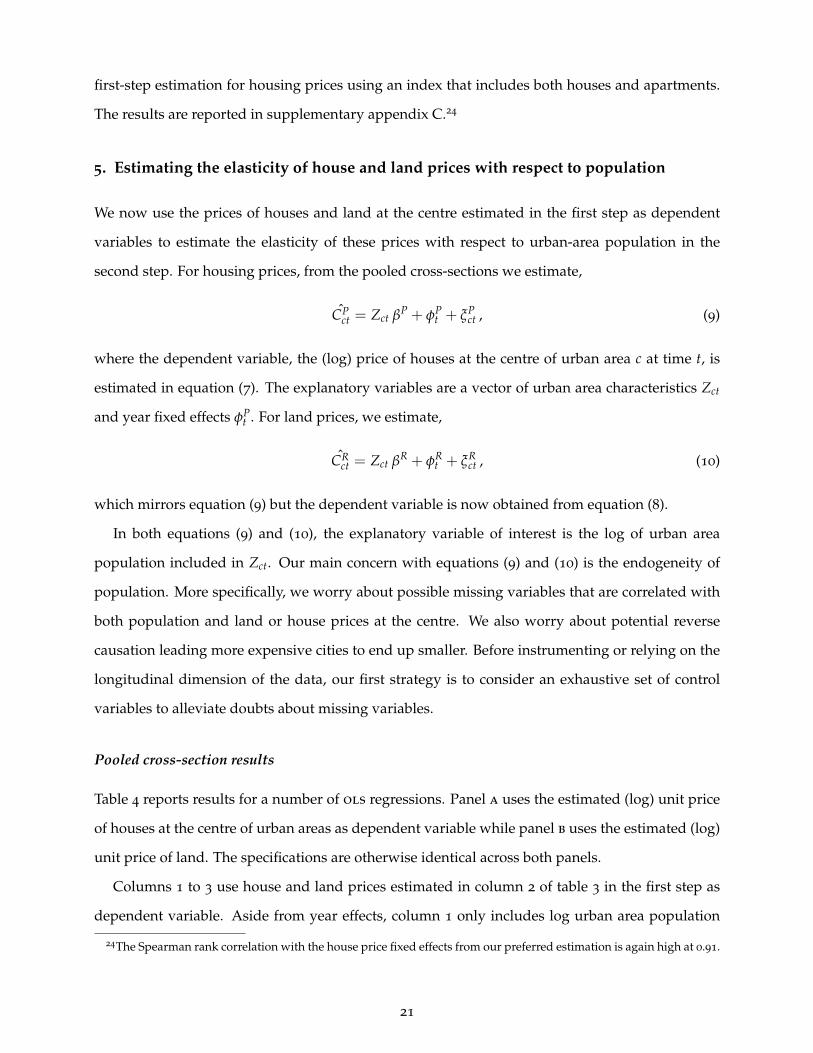
Table 4 reports results for a number of ols regressions. Panel a uses the estimated (log) unit price
of houses at the centre of urban areas as dependent variable while panel b uses the estimated (log)
unit price of land. The specifications are otherwise identical across both panels.
Columns 1 to 3 use house and land prices estimated in column 2 of table 3 in the first step as
dependent variable. Aside from year effects, column 1 only includes log urban area population
24The Spearman rank correlation with the house price fixed effects from our preferred estimation is again high at 0.91.
21

and log area as explanatory variables.25 The estimated population elasticity is 0.217 for house
prices and 0.774 for land prices. Column 2 also includes population growth, log mean income,
log standard deviation of income, and the share of university educated workers. Including these
controls marginally lowers the coefficient on log population, to 0.176 for house prices and to 0.707
for land prices. Column 3 enriches the regression further with 20 geography and geology variables
and two important land use variables, the share of built up area and the log of the average height
of buildings. Adding these extra controls leads to a slight increase of the coefficient on population
in both panels.
Columns 4 to 6 repeat the same pattern of estimation as columns 1 to 3 but use as dependent
variable the fixed effects estimated from column 4 of table 3, a more complete first-step regression,
which includes house or parcel characteristics and a distance effect specific to each urban area in
addition to urban area fixed effects and year fixed effects. Columns 7 to 9 repeat again the same
pattern of estimation but use this time the output of the most complete first-step regression from
column 9 of table 3. In these three columns, the urban area fixed effects are estimated at the first
step conditional on house or parcel characteristics and 34 municipality characteristics, including
their socioeconomic composition, geography, geology, land use, and amenities.
Our preferred ols estimates are in column 8. They suggest an elasticity of house prices with
respect to population of 0.208 and an elasticity of land prices with respect to population of 0.597.
We are interested in estimating the elasticity of house and land prices with respect to population,
all else equal. The estimates of column 7 do not condition out the socio-economic characteristics
of cities. They thus fail to account for the possibility that, among others, larger cities are also more
skilled. We also prefer the estimates of column 8 to those of column 9, which additionally control
for share of land that is built-up and the average height of buildings. While we think that these
two land-use controls are useful proxies for land-use regulations, it may be too extreme to think
of an increase in population in a city that would keep both land use and land area constant as the
relevant thought experiment.
Although we do not report the coefficients on all the control variables in the table, some results
25We generally include the log of land area in our regressions. Besides being a major determinant of the availabilityof land and housing, we also think that the relevant question about urban costs regards their increase following anincrease in population, keeping land area constant. French land use regulations make the expansion of urban boundariesextremely difficult. Below, we nonetheless contrast the results we obtain for urban costs with constant land areas toestimates that allow urban boundaries to adjust.
22
Table 4: The determinants of unit house prices and land values at the centre, OLS regressions
(1) (2) (3) (4) (5) (6) (7) (8) (9)
First-step Only fixed effects | Basic controls | Full set of controls
Controls N Y Ext. | N Y Ext. | N Y Ext.
Panel A. HousesLog population 0.217a 0.176a 0.224a 0.259a 0.215a 0.305a 0.252a 0.208a 0.304a
(0.0210) (0.0142) (0.0283) (0.0276) (0.0187) (0.0378) (0.0262) (0.0179) (0.0368)Log land area -0.151a -0.153a -0.224a -0.114a -0.122a -0.242a -0.143a -0.152a -0.276a
(0.0219) (0.0136) (0.0293) (0.0250) (0.0189) (0.0379) (0.0241) (0.0174) (0.0382)
R2 0.35 0.65 0.72 0.44 0.67 0.73 0.40 0.66 0.73Observations 1,937 1,937 1,937 1,937 1,937 1,937 1,937 1,937 1,937
Panel B. Land parcelsLog population 0.774a 0.707a 0.871a 0.678a 0.604a 0.702a 0.662a 0.597a 0.738a
(0.0464) (0.0435) (0.122) (0.0464) (0.0362) (0.0865) (0.0432) (0.0360) (0.0875)Log land area -0.676a -0.676a -0.881a -0.344a -0.363a -0.505a -0.437a -0.453a -0.630a
(0.0527) (0.0448) (0.133) (0.0464) (0.0379) (0.0905) (0.0445) (0.0372) (0.0934)
R2 0.54 0.64 0.69 0.63 0.75 0.79 0.61 0.73 0.77Observations 1,933 1,933 1,933 1,933 1,933 1,933 1,933 1,933 1,933Notes: The dependent variable is an urban area-year fixed effect estimated in the first step. Columns 1 to 3 use theoutput of column 2 of table 3. Columns 4 to 6 use the output of column 4 of table 3. Columns 7 to 9 use the output ofcolumn 9 of table 3. All regressions include year effects. All reported R2 are within-time. The superscripts a, b, and cindicate significance at 1%, 5%, and 10% respectively. Standard errors clustered at the urban area level are betweenbrackets. For second-step controls, N, Y, and Ext. stand for no further explanatory variables beyond population,land area, and year effects, a set of explanatory variables, and a full set, respectively. Second-step controls includepopulation growth of the urban area (as log of 1 + annualised population growth over the period), income andeducation variables for the urban area (log mean income, log standard deviation, and share of university degrees).Extended controls additionally include the urban-area means of the same 20 geography and geology controls as intable 3 and the same two land use variables (share of built-up land and average height of buildings) used in thesame table.
are worth a brief mention. Most notably, we introduce population growth in the regression to sep-
arate rents today and expectations of future rent increases which are driven by population growth.
Both are included in house prices. A one percentage point of annual population growth is typically
associated with about 10% higher prices for houses. Despite this large effect, including population
growth does not affect the coefficient on population because population and population growth
are only weakly correlated, in keeping with Gibrat’s law. As could be expected, we also find lower
prices in urban areas with greater supply, that is in urban areas where a greater proportion of
the land is built up and where the average height of building is lower. Many of our geographic
controls including the distance to the main rivers and various borders have a significant effect.
They capture broad regional trends in land and housing prices in France. Finally, the coefficient on
23

log mean income is always significant and equal to 1.57 in column 8.
In column 8, the elasticity of land prices is nearly three times as high as the elasticity of house
prices. This is consistent with our findings above that the interquartile range for land prices at
the centre in our preferred estimation is also about two and half times as large as the interquartile
range for house prices at the centre.
Recall that, when we extend our model to allow for a housing construction sector, the popula-
tion elasticity of the price of housing is the product of the population elasticity of the price of land
and the share of land in construction. In the data, the average share of land in the total cost of a
new house is 36% and roughly constant across urban areas and parcel size (Combes et al., 2016).
Using our model, the estimates of column 8 imply an implicit share of land of 35% for old houses.
With the caveat that we compare new constructions with old houses, this is extremely close.
We document in supplementary appendix D that the distance gradients for urban areas with
greater population are steeper. This appendix duplicates table 4 but uses the distance gradient
estimated in the first stage instead of the urban area fixed effect as dependent variable. While
prices at the fringe do not differ much across urban areas, the higher prices at the centre that we
observe in urban areas with greater population are associated with both a greater distance to the
urban fringe and a steeper distance gradient.
Robustness checks
Before implementing alternative estimation strategies, we further explore the robustness of our
second-step ols results.
First, household heterogeneity across urban areas may affect our results.26 Empirical evidence
suggests that more skilled households sort into larger cities (Combes et al., 2008). We expect the
price premium of central locations to be determined by both city population and the socioeconomic
characteristics of this population. While in table 4 we control for a wide range of socioeconomic
characteristics, more complicated interactions may be at work. To assess this possibility, we
duplicate the specifications of table 4 and include interactions between city population and income
or education in supplementary appendix E. This leads to modestly smaller population elasticities.
26In the first step of our estimation, we condition out various socio-economic characteristics of municipalities withinurban areas given our worry that the spatial distribution of heterogeneous households within the urban area may affectthe estimation of gradients and thus of prices at the centre. However, municipal characteristics are measured relativeto the city mean and only condition out household heterogeneity within cities, not differences across cities. We need toaddress heterogeneity both within and between cities.
24
For house prices, our preferred estimation implies an indistinguishable population elasticity of
0.199 instead of 0.208 when including an interaction between population and income. For parcel
prices, the elasticity is 0.572 instead of 0.597 with a similar interaction.
Second, we also duplicate the estimations of panel a of table 4 for housing prices that pertain to
all dwellings instead of only houses. The results are reported in separate appendix F. The estimated
elasticities of the price of central dwellings with respect to city population which are modestly
lower than in table 4. This is likely caused by the lower land intensity of apartments relative to
houses.
Third, we also consider a number of further variants for our preferred specification of column 8
in table 4 in separate appendix G. In particular, we experiment with dependent variables estimated
in the first step with alternative functional forms for distance to the centre, alternative definitions
of a centre, the inclusion of a second centre, separate gradients for each urban area and year,
and interactions between municipal income and distance to the centre. We also use alternative
samples which exclude the 25% cheapest municipalities or the 25% closest municipalities to the
centre in the first step to deal with potential selection problems for transactions. We also consider
alternative weighting schemes in the estimation and alternative second-step samples that eliminate
observations with negative growth. Because we rely in our second step on a dependent variable
that is estimated (with error) in a first step, we also experiment with fgls and wls techniques to
explicitly account for this measurement error (see separate appendix H for further explanations).
Finally, instead of using a two-step procedure, we can also estimate everything in one step. While
we estimate sometimes smaller or larger population elasticities, the magnitudes are in general close
and supportive of our baseline findings.
Instrumental-variable estimates
To repeat, in the estimation of equations (9) and (10) we are concerned with the endogeneity of
population. We expect the main source of endogeneity to arise from the existence of missing
variables that are correlated with population and affect land or house prices through some other
channel. Another possible source of endogeneity is reverse causation: population may become
larger in cheaper cities. Both sources of endogeneity can be addressed through instrumental
variables. Because land area is highly correlated with population, we need to instrument both
variables.
25

We use two sets of instruments. Our first set of instruments is suggested by our model where
exogenous amenities in a city attract population without otherwise affecting the demand or supply
of housing in this city. More specifically, we use a measure of temperatures in January, a count of
hotel rooms, and the share of budget hotels. Our measure of climate is motivated by the literature
on urban growth. This literature shows that January temperatures is a strong predictor of urban
growth and thus of urban population in the long run (Duranton and Puga, 2014). A count of hotel
rooms is in the spirit of Carlino and Saiz (2008) who argue that tourism visits provide a summary
proxy for all amenities in a city. We prefer to focus on budget hotels since higher-end hotels in
France arguably cater predominantly to the needs of business travellers.
Our second set of instruments consists of long lags of urban population and density constructed
from population and area data from 1831, 1851, and 1881. This instrumental strategy follows a
long tradition in the urban literature where city population is instrumented with past values of
the same variable to estimate agglomeration effects (Combes and Gobillon, 2015). We expect these
predictors of city population to be immune from reverse causation and from the effects of more
recent shocks affecting both population and prices.
While we can make the case that these instruments are strong enough predictors of contem-
poraneous city population, they might still be correlated with land or housing prices through
some other demand or supply channels. For instance, amenities may induce residents to consume
more (or less) housing. To address this worry, we can control extensively for the characteristics of
municipalities and urban areas to preclude these sources of correlation with the error term. We also
note that long population lags and amenities rely on different sources of variation in the data to
predict contemporaneous populations. For instance, the correlation between January temperatures
and the other instruments is always below 0.10. Obtaining statistically similar coefficients from
these different instruments is reassuring.
In separate appendix I, we provide further details about our iv strategy and report results for
both house and land prices. For house prices, most of our estimates of the population elasticity are
between 0.20 and 0.27 with a few exceptions above or below. For land prices, most of the estimates
of the population elasticity are between 0.60 and 0.80. In both cases, this is moderately larger than
our preferred ols estimates of 0.208 and 0.597 but comparable to other estimates reported in table
4 and in the separate appendix. We conclude that our iv results are supportive of our baseline ols
results.
26
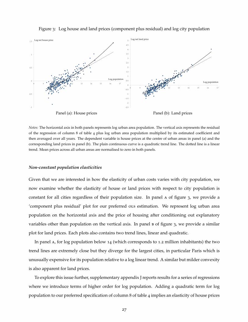
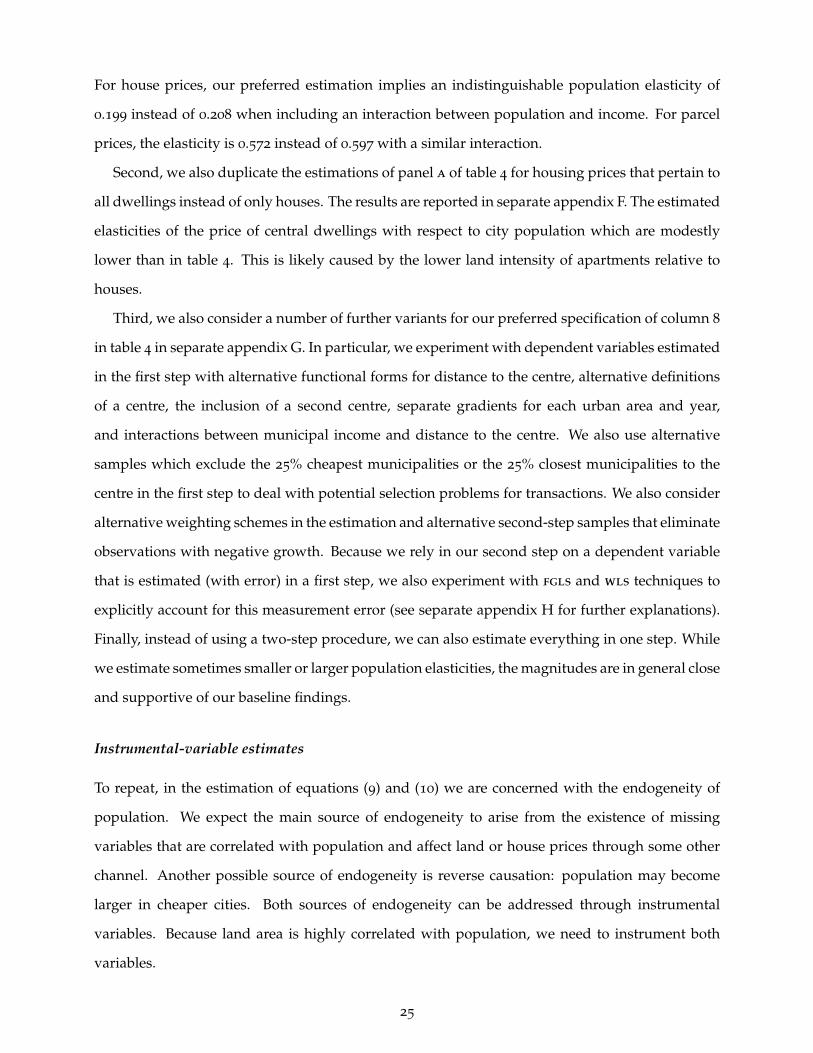
Figure 3: Log house and land prices (component plus residual) and log city population
‐1
‐0.5
0
0.5
1
1.5
8 9 10 11 12 13 14 15 16 17
Log net house price
Log population
‐2.5
‐2
‐1.5
‐1
‐0.5
0
0.5
1
1.5
2
2.5
3
3.5
4
4.5
5
8 9 10 11 12 13 14 15 16 17
Log net land price
Log population
Panel (a): House prices Panel (b): Land prices
Notes: The horizontal axis in both panels represents log urban area population. The vertical axis represents the residualof the regression of column 8 of table 4 plus log urban area population multiplied by its estimated coefficient andthen averaged over all years. The dependent variable is house prices at the centre of urban areas in panel (a) and thecorresponding land prices in panel (b). The plain continuous curve is a quadratic trend line. The dotted line is a lineartrend. Mean prices across all urban areas are normalised to zero in both panels.
Non-constant population elasticities
Given that we are interested in how the elasticity of urban costs varies with city population, we
now examine whether the elasticity of house or land prices with respect to city population is
constant for all cities regardless of their population size. In panel a of figure 3, we provide a
‘component plus residual’ plot for our preferred ols estimation. We represent log urban area
population on the horizontal axis and the price of housing after conditioning out explanatory
variables other than population on the vertical axis. In panel b of figure 3, we provide a similar
plot for land prices. Each plots also contains two trend lines, linear and quadratic.
In panel a, for log population below 14 (which corresponds to 1.2 million inhabitants) the two
trend lines are extremely close but they diverge for the largest cities, in particular Paris which is
unusually expensive for its population relative to a log linear trend. A similar but milder convexity
is also apparent for land prices.
To explore this issue further, supplementary appendix J reports results for a series of regressions
where we introduce terms of higher order for log population. Adding a quadratic term for log
population to our preferred specification of column 8 of table 4 implies an elasticity of house prices
27

with respect to population of 0.205 for an urban area with 100,000 inhabitants, an elasticity of 0.288
for an urban area with a million inhabitants, and 0.378 for an urban area with the same population
as Paris. The other specifications yield roughly similar estimates. Again, we must remain cautious
about this non-linearity because it is driven only by the three or four largest cities.
To summarise our findings so far, our preferred estimate for the elasticity of house prices at the
centre of urban areas with respect to population is 0.208. Alternative ols and iv estimates for this
elasticity reported in table 4 and in the separate appendix are mostly in the 0.15-0.30 range. We
also find that this elasticity possibly increases with population for the largest urban areas. The
estimates for land prices are equally stable and consistent with those for house prices.
Estimates for alternative time horizons
All our specifications so far include land area as a control. Given the current institutional frame-
work in France, which strongly encourages in-filling but discourages the expansion of the urban
fringe, we view the population elasticities of land and house prices conditional on urban area as
the relevant benchmarks to think about urban costs.
In the very long-run, the current institutional framework may change and allow urban areas
to expand physically with population. In separate appendix K, we duplicate table 4 and estimate
the same population elasticity as previously without including land area. We find much smaller
coefficients for population equal to or slightly larger than the sum of the population coefficients
and the (negative) land area coefficients estimated in table 4. This is consistent with an estimated
coefficient of about 0.7 for log population when we regress log land area on log population. For
our preferred specification but without including land area, we estimate a population elasticity of
house prices equal to 0.109 instead of 0.208 previously.
At the other extreme, it is also interesting to estimate urban costs over a short time horizon,
perhaps before the housing stock fully adjusts to population changes.27 For that purpose, we can
estimate equation (10) in the within dimension using observations every odd year between 2000
and 2012. We can also estimate this equation in difference using 2012 and 2000.28 These two
27A change in demand may take time to be perceived by house builders. Obtaining a building permit takes time andbuilding a house also takes time. Beyond this, new housing often requires a change in the zoning designation (conver-sion from agricultural to residential or from commercial/manufacturing to residential). These changes are infrequentin France – every 20 years or so, see the example of Lyon discussed at https://www.grandlyon.com/fileadmin/user_upload/media/pdf/espace-presse/dp/2017/20170911_dp_pluh.pdf (consulted on 22 December 2017).
28We do not use land price data here because they are only available for a short time period (2006-2012) instead of2000-2012 for house price data.
28
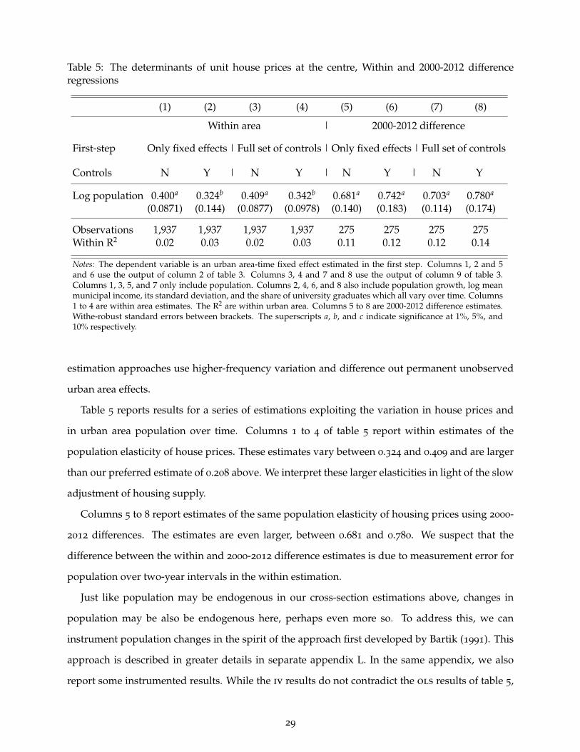
Table 5: The determinants of unit house prices at the centre, Within and 2000-2012 differenceregressions
(1) (2) (3) (4) (5) (6) (7) (8)
Within area | 2000-2012 difference
First-step Only fixed effects | Full set of controls | Only fixed effects | Full set of controls
Controls N Y | N Y | N Y | N Y
Log population 0.400a 0.324b 0.409a 0.342b 0.681a 0.742a 0.703a 0.780a
(0.0871) (0.144) (0.0877) (0.0978) (0.140) (0.183) (0.114) (0.174)
Observations 1,937 1,937 1,937 1,937 275 275 275 275Within R2 0.02 0.03 0.02 0.03 0.11 0.12 0.12 0.14
Notes: The dependent variable is an urban area-time fixed effect estimated in the first step. Columns 1, 2 and 5and 6 use the output of column 2 of table 3. Columns 3, 4 and 7 and 8 use the output of column 9 of table 3.Columns 1, 3, 5, and 7 only include population. Columns 2, 4, 6, and 8 also include population growth, log meanmunicipal income, its standard deviation, and the share of university graduates which all vary over time. Columns1 to 4 are within area estimates. The R2 are within urban area. Columns 5 to 8 are 2000-2012 difference estimates.Withe-robust standard errors between brackets. The superscripts a, b, and c indicate significance at 1%, 5%, and10% respectively.
estimation approaches use higher-frequency variation and difference out permanent unobserved
urban area effects.
Table 5 reports results for a series of estimations exploiting the variation in house prices and
in urban area population over time. Columns 1 to 4 of table 5 report within estimates of the
population elasticity of house prices. These estimates vary between 0.324 and 0.409 and are larger
than our preferred estimate of 0.208 above. We interpret these larger elasticities in light of the slow
adjustment of housing supply.
Columns 5 to 8 report estimates of the same population elasticity of housing prices using 2000-
2012 differences. The estimates are even larger, between 0.681 and 0.780. We suspect that the
difference between the within and 2000-2012 difference estimates is due to measurement error for
population over two-year intervals in the within estimation.
Just like population may be endogenous in our cross-section estimations above, changes in
population may be also be endogenous here, perhaps even more so. To address this, we can
instrument population changes in the spirit of the approach first developed by Bartik (1991). This
approach is described in greater details in separate appendix L. In the same appendix, we also
report some instrumented results. While the iv results do not contradict the ols results of table 5,
29
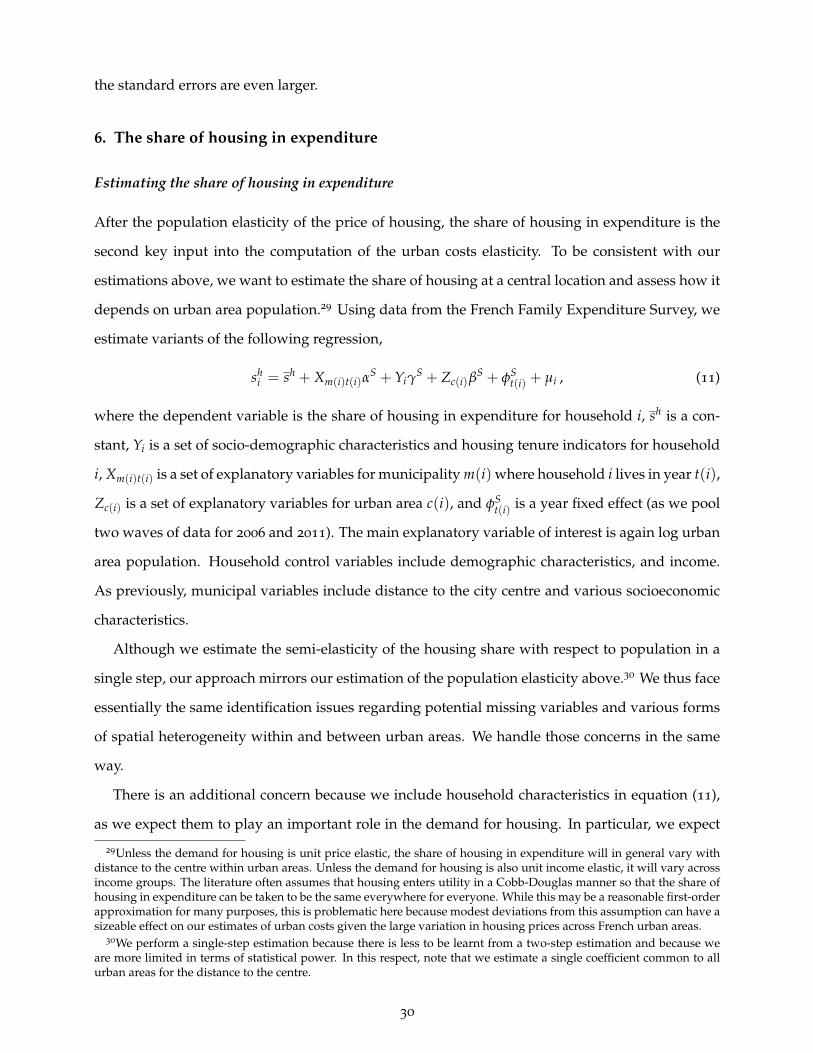
the standard errors are even larger.
6. The share of housing in expenditure
Estimating the share of housing in expenditure
After the population elasticity of the price of housing, the share of housing in expenditure is the
second key input into the computation of the urban costs elasticity. To be consistent with our
estimations above, we want to estimate the share of housing at a central location and assess how it
depends on urban area population.29 Using data from the French Family Expenditure Survey, we
estimate variants of the following regression,
shi = sh + Xm(i)t(i)α
S + YiγS + Zc(i)β
S + φSt(i) + µi , (11)
where the dependent variable is the share of housing in expenditure for household i, sh is a con-
stant, Yi is a set of socio-demographic characteristics and housing tenure indicators for household
i, Xm(i)t(i) is a set of explanatory variables for municipality m(i) where household i lives in year t(i),
Zc(i) is a set of explanatory variables for urban area c(i), and φSt(i) is a year fixed effect (as we pool
two waves of data for 2006 and 2011). The main explanatory variable of interest is again log urban
area population. Household control variables include demographic characteristics, and income.
As previously, municipal variables include distance to the city centre and various socioeconomic
characteristics.
Although we estimate the semi-elasticity of the housing share with respect to population in a
single step, our approach mirrors our estimation of the population elasticity above.30 We thus face
essentially the same identification issues regarding potential missing variables and various forms
of spatial heterogeneity within and between urban areas. We handle those concerns in the same
way.
There is an additional concern because we include household characteristics in equation (11),
as we expect them to play an important role in the demand for housing. In particular, we expect
29Unless the demand for housing is unit price elastic, the share of housing in expenditure will in general vary withdistance to the centre within urban areas. Unless the demand for housing is also unit income elastic, it will vary acrossincome groups. The literature often assumes that housing enters utility in a Cobb-Douglas manner so that the share ofhousing in expenditure can be taken to be the same everywhere for everyone. While this may be a reasonable first-orderapproximation for many purposes, this is problematic here because modest deviations from this assumption can have asizeable effect on our estimates of urban costs given the large variation in housing prices across French urban areas.
30We perform a single-step estimation because there is less to be learnt from a two-step estimation and because weare more limited in terms of statistical power. In this respect, note that we estimate a single coefficient common to allurban areas for the distance to the centre.
30

Table 6: The share of housing in expenditure for homeowners and renters
(1) (2) (3) (4) (5) (6) (7) (8)Log population 0.028a 0.031a 0.037a 0.039a 0.036a 0.047a 0.067a 0.048a
(0.001) (0.001) (0.005) (0.007) (0.007) (0.011) (0.010) (0.008)Log land area -0.011 -0.017b -0.020a -0.025b -0.043a -0.025a
(0.007) (0.007) (0.006) (0.010) (0.010) (0.008)Population growth 2.767a 2.694a 2.503a 2.521a 2.121a 2.502a
(0.562) (0.640) (0.679) (0.665) (0.692) (0.649)Log distance to city centre -0.008c -0.008 -0.006b -0.003 -0.008a -0.013a -0.008a
(0.005) (0.005) (0.003) (0.003) (0.003) (0.003) (0.003)Log income -0.282a -0.284a -0.283a -0.286a -0.170a -0.286a -0.286a -0.286a
(0.013) (0.012) (0.012) (0.011) (0.012) (0.011) (0.011) (0.011)
First-stage statistic 158.0 112.5 6.6 17.2Overidentification p-value 0.09 0.03 0.00
InstrumentsEducational level (degree) XUrban population in 1831 X XConsumption amenities X XLocal controls No No No Yes Yes Yes Yes YesR2 0.56 0.56 0.56 0.57
Note All R2 are within time. 8,446 observations in each regression corresponding to 197 urban areas. Standard errors are clustered at theurban area level. a: significant at 1% level; b: significant at 5% level; c: significant at 10% level. All variables are centred and the estimatedconstant, which corresponds to the expenditure share in a city of average size (2.99 million inhabitants, 3.17 million with weights), takesthe value 0.325 in all specifications (weighted and unweighted). Regressions are weighted with sampling weights and include: age andindicator variables for year 2011 (ref. 2006), homeowner (ref. renter), living in couple within the dwelling (ref. single), one child, twochildren, three children and more (ref. no child). Local controls include the same geography variables for urban areas as in table 4 and thesame geology, land use, and amenity variables at the municipality level as in table 3. OLS for columns (1) to (4). IV estimated with limitedinformation maximum likelihood (LIML) in columns (5) (income instrumented), (6) and (7) (population instrumented) and (8) (incomeand population instrumented). The first-stage statistics is the Kleibergen-Paap rk Wald F. The critical value for 10% maximal LIML size ofStock and Yogo (2005) weak identification test is 4.45 for column (5), 16.38 for column (6), 3.50 for column (7), and 3.42 for column (8).
The education instruments are five indicator variables corresponding to PhD and elite institution degree, master, lower university
degree, high school and technical degree, lower technical degree, and primary school (reference). Amenities instruments are: January
temperature, the log number of hotel rooms and the share of one-star hotel rooms.
housing decisions to be driven by permanent income, while we only observe current income.
Because income and population are possibly related (be it only because of agglomeration effects),
this may affect the estimates of our coefficient of interest. Like previous literature (e.g., Glaeser,
Kahn, and Rappaport, 2008), we can instrument household income by education.
Baseline results
Table 6 reports results for the pooled sample of homeowners and renters in the French Family
Expenditure Surveys for 2006 and 2011. Column 1 regresses the share of housing in expenditure on
household demographic characteristics, (log) household income, and (log) urban area population.
31

We estimate a coefficient on city population of 0.028. Column 2 also includes distance to the city
centre. Columns 3 and 4 further enrich the regression by including log land area, population
growth, and a number of further controls to condition out the socioeconomic characteristics of
urban areas. The coefficient on population increases slightly to 0.039.31 Column 5 duplicates
column 4 but instruments for income using five indicator variables for educational achievement.
This lowers the magnitude of the coefficient on income but does not appear to affect the rest of the
regression. In particular, the coefficient on population in column 5 differs only marginally from its
counterpart in column 4.
Column 6 of table 6 instruments contemporaneous urban area population by urban area popu-
lation in 1831. The point estimate on population modestly rises from 0.039 with ols in column 4 to
0.047. These two coefficients are only about one standard deviation apart. Column 7 instruments
population with urban area amenities. More specifically, we use, as previously, the overall number
of hotel rooms and the number of low-end hotel rooms per population.32 This leads to a slightly
higher coefficient on city population of 0.067. While this larger coefficient does not really affect
our conclusions as we show below, we should keep in mind that the instruments are weaker in
that case. Finally, column 8 uses both amenities and past population as instruments to estimate a
coefficient of 0.048 for population.
These small variations in the coefficient for urban area population make no economically mean-
ingful difference to our final results. With a mean share of housing in expenditure of 0.325 for
a mean urban area of 3.17 million inhabitants, our preferred coefficient of 0.048 from column 8
implies a share of housing in expenditure of 0.390 for a city with the same population as Paris and
a share of 0.159 for an urban area with only 100,000 inhabitant. Retaining a population coefficient
of 0.028 as in column 1 rather than 0.048 implies a share of housing in expenditure of 0.363 for a
city with the same population as Paris. At the other extreme, a population coefficient of 0.067 as in
column 7 implies a housing share of 0.415 for the same hypothetical city.
31Most of the change in the coefficient on city population between columns 2 and 3 of table 6 is due to the inclusionof land area into the regression. Recall that land area is strongly positively correlated with city population.
32When using amenities as instruments at the urban area level, we include a measure of the same variables at themunicipal level as explanatory variables in the regression. All our municipal explanatory variables are centred relativetheir urban area means. Moreover, we keep in mind that the regressions of table 6 exploit data from only 197 urbanareas instead of 277 previously when estimating the elasticity of house and land prices with respect to population.
32

Robustness checks
In separate appendix M, we report results for a number of robustness checks. In particular, we
replicate the results of table 6 for homeowners and renters separately. For our preferred estimation,
we find modest differences for the coefficient on city population for renters and homeowners of
about 0.02 apart. This is small and statistically insignificant. We also discuss a range of further
supplementary estimations which also instrument for land area in addition to population or
use directly household education in reduced form as a control instead of using it as instrument
for income. We also provide evidence to alleviate worries about possible non-linearities in the
relationship between the share of income in housing and urban area population.
7. The elasticity of urban costs with respect to population
With both the elasticity of house prices at the centre with respect to population and the share
of housing in household expenditure now at hand, we can compute their product to obtain the
elasticity of urban costs with respect to city population, as per equation (6). Because both quantities
possibly vary with city population, the elasticity of urban costs will also vary with population. To
illustrate our results, we consider three hypothetical cities. A small city with 100,000 inhabitants,
a larger city with a million inhabitants, and a large city with a population equal to that of Paris,
slightly above 12 million.
Starting with the elasticity of house prices with respect to city population, we consider four
different situations in panel a of table 7. First, we use our preferred ols estimate of 0.208 from
column 8 of table 4 for our baseline calculation. Among all the ols cross-sectional estimates
reported in the rest of table 4 and the separate appendix, the smallest is equal to 0.134 and
the largest is 0.306. These extreme values, which are respectively 36% smaller and 47% larger
than our baseline, provide useful bounds.33 Second, we also use estimates for which we allow
the population elasticity of house prices to vary with city population. These estimates imply a
population elasticity of house prices of 0.205 for a small city, an elasticity of 0.288 for a city with
a million inhabitants, and an elasticity of 0.378 for a large city like Paris. Finally, we consider two
more extreme cases that rely on values of 0.780 and 0.109 for the population elasticity of house
33Alternatively, if we consider the 92 estimates for the coefficient on log population in all the specifications reportedin table 4 and in the separate appendix (ols and iv) which include log population and log area, their mean is 0.224 andthe standard deviation is 0.052. Considering two standard deviations around this average comes reasonably close to thevalues of 0.134 and 0.306 retained in our bounding exercise.
33
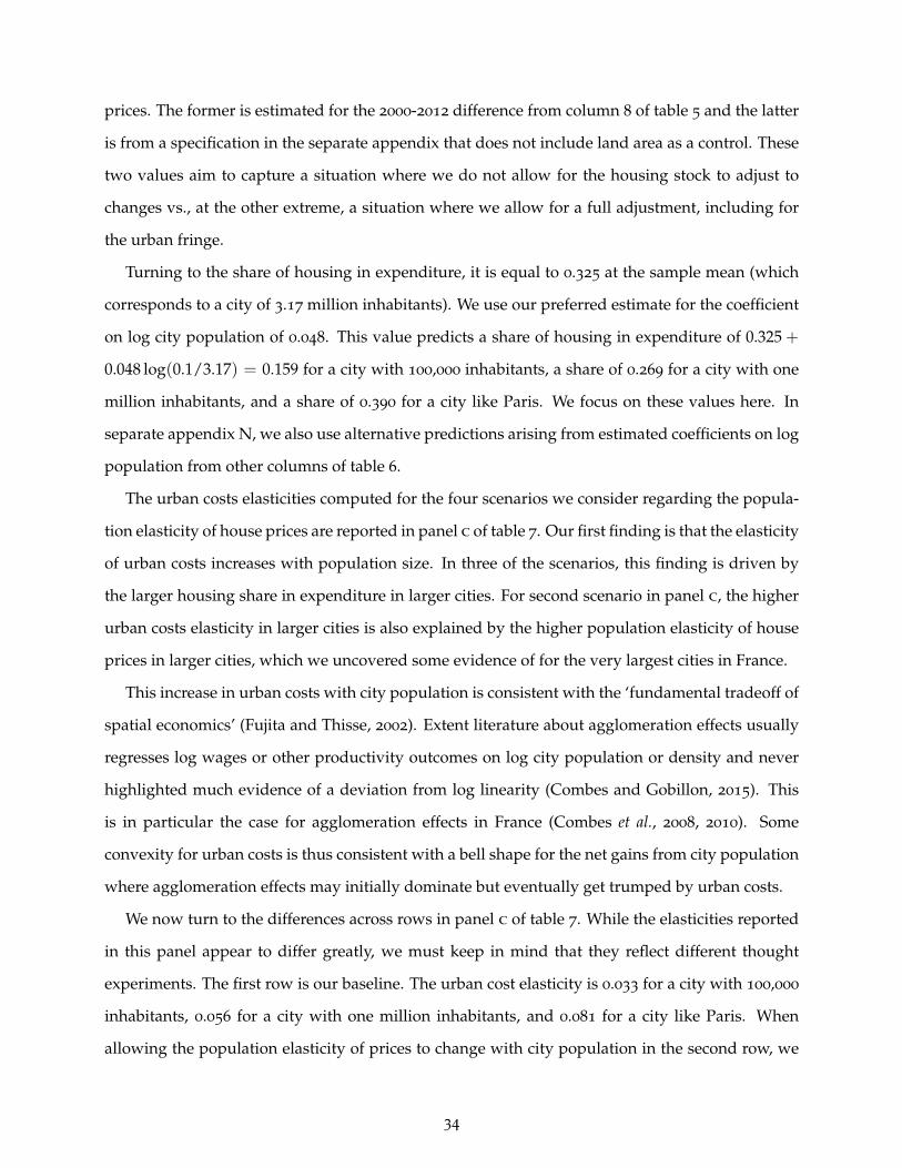
prices. The former is estimated for the 2000-2012 difference from column 8 of table 5 and the latter
is from a specification in the separate appendix that does not include land area as a control. These
two values aim to capture a situation where we do not allow for the housing stock to adjust to
changes vs., at the other extreme, a situation where we allow for a full adjustment, including for
the urban fringe.
Turning to the share of housing in expenditure, it is equal to 0.325 at the sample mean (which
corresponds to a city of 3.17 million inhabitants). We use our preferred estimate for the coefficient
on log city population of 0.048. This value predicts a share of housing in expenditure of 0.325 +
0.048 log(0.1/3.17) = 0.159 for a city with 100,000 inhabitants, a share of 0.269 for a city with one
million inhabitants, and a share of 0.390 for a city like Paris. We focus on these values here. In
separate appendix N, we also use alternative predictions arising from estimated coefficients on log
population from other columns of table 6.
The urban costs elasticities computed for the four scenarios we consider regarding the popula-
tion elasticity of house prices are reported in panel c of table 7. Our first finding is that the elasticity
of urban costs increases with population size. In three of the scenarios, this finding is driven by
the larger housing share in expenditure in larger cities. For second scenario in panel c, the higher
urban costs elasticity in larger cities is also explained by the higher population elasticity of house
prices in larger cities, which we uncovered some evidence of for the very largest cities in France.
This increase in urban costs with city population is consistent with the ‘fundamental tradeoff of
spatial economics’ (Fujita and Thisse, 2002). Extent literature about agglomeration effects usually
regresses log wages or other productivity outcomes on log city population or density and never
highlighted much evidence of a deviation from log linearity (Combes and Gobillon, 2015). This
is in particular the case for agglomeration effects in France (Combes et al., 2008, 2010). Some
convexity for urban costs is thus consistent with a bell shape for the net gains from city population
where agglomeration effects may initially dominate but eventually get trumped by urban costs.
We now turn to the differences across rows in panel c of table 7. While the elasticities reported
in this panel appear to differ greatly, we must keep in mind that they reflect different thought
experiments. The first row is our baseline. The urban cost elasticity is 0.033 for a city with 100,000
inhabitants, 0.056 for a city with one million inhabitants, and 0.081 for a city like Paris. When
allowing the population elasticity of prices to change with city population in the second row, we
34
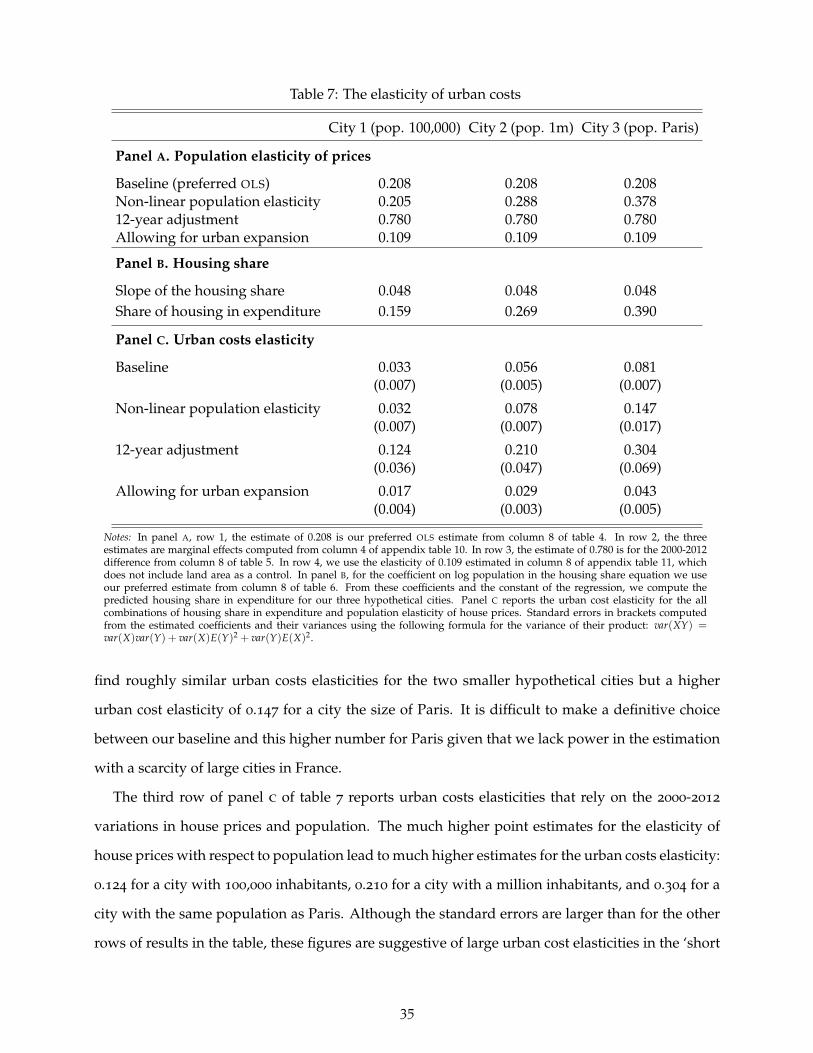
Table 7: The elasticity of urban costs
City 1 (pop. 100,000) City 2 (pop. 1m) City 3 (pop. Paris)
Panel A. Population elasticity of prices
Baseline (preferred OLS) 0.208 0.208 0.208Non-linear population elasticity 0.205 0.288 0.37812-year adjustment 0.780 0.780 0.780Allowing for urban expansion 0.109 0.109 0.109
Panel B. Housing share
Slope of the housing share 0.048 0.048 0.048Share of housing in expenditure 0.159 0.269 0.390
Panel C. Urban costs elasticity
Baseline 0.033 0.056 0.081(0.007) (0.005) (0.007)
Non-linear population elasticity 0.032 0.078 0.147(0.007) (0.007) (0.017)
12-year adjustment 0.124 0.210 0.304(0.036) (0.047) (0.069)
Allowing for urban expansion 0.017 0.029 0.043(0.004) (0.003) (0.005)
Notes: In panel A, row 1, the estimate of 0.208 is our preferred OLS estimate from column 8 of table 4. In row 2, the threeestimates are marginal effects computed from column 4 of appendix table 10. In row 3, the estimate of 0.780 is for the 2000-2012difference from column 8 of table 5. In row 4, we use the elasticity of 0.109 estimated in column 8 of appendix table 11, whichdoes not include land area as a control. In panel B, for the coefficient on log population in the housing share equation we useour preferred estimate from column 8 of table 6. From these coefficients and the constant of the regression, we compute thepredicted housing share in expenditure for our three hypothetical cities. Panel C reports the urban cost elasticity for the allcombinations of housing share in expenditure and population elasticity of house prices. Standard errors in brackets computedfrom the estimated coefficients and their variances using the following formula for the variance of their product: var(XY) =var(X)var(Y) + var(X)E(Y)2 + var(Y)E(X)2.
find roughly similar urban costs elasticities for the two smaller hypothetical cities but a higher
urban cost elasticity of 0.147 for a city the size of Paris. It is difficult to make a definitive choice
between our baseline and this higher number for Paris given that we lack power in the estimation
with a scarcity of large cities in France.
The third row of panel c of table 7 reports urban costs elasticities that rely on the 2000-2012
variations in house prices and population. The much higher point estimates for the elasticity of
house prices with respect to population lead to much higher estimates for the urban costs elasticity:
0.124 for a city with 100,000 inhabitants, 0.210 for a city with a million inhabitants, and 0.304 for a
city with the same population as Paris. Although the standard errors are larger than for the other
rows of results in the table, these figures are suggestive of large urban cost elasticities in the ‘short
35

run’ before the supply of housing can adjust (which may take many years in the French context).
In turn, these findings are indicative of potentially large frictions in the housing market. When
population takes extremely long to adjust following the economic shocks that affect cities, workers
may end up residing where housing is affordable and not where they are the most economically
productive or where amenities are the highest.
Finally, the last row of panel c of table 7 allows for a full adjustment of cities to population
growth, including a physical expansion. With this scenario, the elasticity of urban costs with
respect to city population is 0.017 for a city with 100,000 inhabitants, 0.029 for a city with a million
inhabitants, and 0.043 for a city of the size of Paris. These figures indicate that when cities can
adjust their physical footprint, the costs of urban expansion are low. With an elasticity of wages
with respect to city population of about 0.02-0.03 (Combes et al., 2008), our results indicate that in
the bell shape associated with the fundamental tradeoff of spatial economics is relatively flat in
that case. Cities appear to operate close to net constant returns when they can fully adjust.
If we take seriously the notion of a spatial equilibrium across cities as described in the model,
the difference between the urban cost elasticity and the agglomeration elasticity should be equal
to the change in willingness to pay for amenities as city population increases. This difference is
negative for small cities and becomes positive for large cities. In a spatial equilibrium framework,
we should interpret our results as indicating that amenities are getting mildly better as cities of a
larger size are considered (as wages increase less fast than urban costs). The key is nonetheless the
small size of these effects, an interpretation consistent with the results of Albouy (2008, 2016) for
us cities.
8. Conclusion
This paper develops a new methodology to estimate the elasticity of urban costs with respect to
city population. Our model derives this elasticity as the product of two terms: the share of housing
in consumer expenditure and the elasticity of the price of houses at the centre of cities with respect
to city population.
Using data for French urban areas, our preferred estimate of the elasticity of house prices with
respect to city population is 0.208 with most alternative estimates being between 0.15 and 0.30 in
pooled cross section. Finally, we estimate that the share of housing in expenditure varies from
36
0.159 in small urban areas with 100,000 inhabitants to 0.409 in a city with more than 12 million
inhabitants like Paris.
These findings imply elasticities of urban costs from about 0.033 for an urban area with 100,000
inhabitants to 0.081 for an urban area of the size of Paris. These figures refer to the effect of
an increase in population, keeping land area constant (i.e., higher density). We think these are
the relevant magnitudes to consider in France during our study period as planning regulations
strongly discourage urban expansion. Allowing land area to adjust following population increases
in cities leads to urban costs elasticities which are smaller by a factor of about two. Looking at
changes within cities over time leads instead to larger estimates of the urban cost elasticity as
housing supply takes long to adjust.
Given the existence of agglomeration benefits with apparently a constant elasticity of urban
wages with respect to city population at around 0.02-0.03 for France, higher elasticities of urban
costs in larger cities are consistent with the ‘fundamental tradeoff of spatial economics’ according
to which cities face a region of increasing returns where agglomeration gains dominate urban costs
followed by a region of decreasing returns as we consider larger population sizes. This tradeoff
may play nonetheless only a minor role in explaining the future evolution of French cities. In the
short run, the adjustment of housing supply is expected to play a major role as house prices are
fairly sensitive to population changes over a period or a decade or so. In the long run, the bell
shape of net urban gains as a function of population is relatively flat so that cities may deviate
from their efficient size without leading to large economic losses.
37

References
Albouy, David. 2008. Are big cities really bad places to live? Improving quality-of-life estimatesacross cities. Working Paper 14472, National Bureau of Economic Research.
Albouy, David. 2009. The unequal geographic burden of federal taxation. Journal of PoliticalEconomy 117(4):635–667.
Albouy, David. 2016. What are cities worth? Land rents, local productivity, and the total value ofamenities. Review of Economics and Statistics 98(3):forthcoming.
Albouy, David and Gabriel Ehrlich. 2012. Metropolitan land values and housing productivity.Working Paper 18110, National Bureau of Economic Research.
Alonso, William. 1964. Location and Land Use; Toward a General Theory of Land Rent. Cambridge, ma:Harvard University Press.
Au, Chun-Chung and J. Vernon Henderson. 2006. Are Chinese cities too small? Review of EconomicStudies 73(3):549–576.
Bartik, Timothy. 1991. Who Benefits from State and Local Economic Development Policies? Kalamazoo(mi): W.E. Upjohn Institute for Employment Research.
Baum-Snow, Nathaniel and Ronni Pavan. 2012. Understanding the city size wage gap. Review ofEconomic Studies 79(1):88–127.
Behrens, Kristian, Gilles Duranton, and Frédéric Robert-Nicoud. 2014. Productive cities: Sorting,selection, and agglomeration. Journal of Political Economy 122(3):507–553.
Bleakley, Hoyt and Jeffrey Lin. 2012. Portage and path dependence. Quarterly Journal of Economics127(2):587–644.
Carlino, Gerald A. and Albert Saiz. 2008. Beautiful city: Leisure amenities and urban growth.Federal Reserve Bank of Philadelphia Working Paper No. 08-22.
Clark, Colin. 1951. Urban population densities. Journal of the Royal Statistical Association Series A114(4):490–496.
Colwell, Peter F. and C. F. Sirmans. 1978. Area, time, centrality and the value of urban land. LandEconomics 54(4):504–519.
Combes, Pierre-Philippe, Gilles Duranton, and Laurent Gobillon. 2008. Spatial wage disparities:Sorting matters! Journal of Urban Economics 63(2):723–742.
Combes, Pierre-Philippe, Gilles Duranton, and Laurent Gobillon. 2016. The production functionfor housing: Evidence from France. Processed, Wharton School, University of Pennsylvania.
Combes, Pierre-Philippe, Gilles Duranton, Laurent Gobillon, Diego Puga, and Sébastien Roux.2012. The productivity advantages of large cities: Distinguishing agglomeration from firmselection. Econometrica 80(6):2543–2594.
Combes, Pierre-Philippe, Gilles Duranton, Laurent Gobillon, and Sébastien Roux. 2010. Estimatingagglomeration economies with history, geology, and worker effects. In Edward L. Glaeser (ed.)The Economics of Agglomeration. Cambridge (ma): National Bureau of Economic Research, 15–65.
38

Combes, Pierre-Philippe and Laurent Gobillon. 2015. The empirics of agglomeration economies. InGilles Duranton, Vernon Henderson, and William Strange (eds.) Handbook of Regional and UrbanEconomics, volume 5A. Amsterdam: Elsevier, 247–348.
Commissariat Général au Développement Durable. 2015. RéférenceS: Les Comptes des Transports en2014. Paris: Ministère de l’Ecologie, du Développement Durable, des Transports et du Logement.
Davis, Morris A. and Jonathan Heathcote. 2007. The price and quantity of residential land in theUnited States. Journal of Monetary Economics 54(8):2595–2620.
Davis, Morris A. and Michael G. Palumbo. 2008. The price of residential land in large US cities.Journal of Urban Economics 63(1):352–384.
Desmet, Klaus and J. Vernon Henderson. 2015. The geography of development within countries. InGilles Duranton, Vernon Henderson, and William Strange (eds.) Handbook of Regional and UrbanEconomics, volume 5B. Amsterdam: Elsevier, 1457–1517.
Duranton, Gilles and Diego Puga. 2014. The growth of cities. In Philippe Aghion and StevenDurlauf (eds.) Handbook of Economic Growth, volume 2. Amsterdam: North-Holland, 781–853.
Duranton, Gilles and Diego Puga. 2015. Urban land use. In Gilles Duranton, J. Vernon Henderson,and William C. Strange (eds.) Handbook of Regional and Urban Economics, volume 5A. Amsterdam:North-Holland, 467–560.
Duranton, Gilles and Matthew A. Turner. 2016. Urban form and driving: Evidence from US cities.Processed, Wharton School, University of Pennsylvania.
Fujita, Masahisa and Hideaki Ogawa. 1982. Multiple equilibria and structural transition of non-monocentric urban configurations. Regional Science and Urban Economics 12(2):161–196.
Fujita, Masahisa and Jacques-François Thisse. 2002. Economics of Agglomeration: Cities, IndustrialLocation, and Regional Growth. Cambridge: Cambridge University Press.
Glaeser, Edward L., Matthew E. Kahn, and Jordan Rappaport. 2008. Why do the poor live in cities?The role of public transportation. Journal of Urban Economics 63(1):1–24.
Handbury, Jessie and David E. Weinstein. 2015. Goods prices and availability in cities. Review ofEconomic Studies 82(1):258–296.
Henderson, J. Vernon. 1974. The sizes and types of cities. American Economic Review 64(4):640–656.
Henderson, Vernon. 2002. Urban primacy, external costs, and the quality of life. Resource andEnergy Economics 24(1):95–106.
Kline, Patrick and Enrico Moretti. 2015. People, places and public policy: Some simple welfareeconomics of local economic development programs. Annual Review of Economics 9(0):forthcom-ing.
Mills, Edwin S. 1967. An aggregative model of resource allocation in a metropolitan area. AmericanEconomic Review (Papers and Proceedings) 57(2):197–210.
Muth, Richard F. 1969. Cities and Housing. Chicago: University of Chicago Press.
Puga, Diego. 2010. The magnitude and causes of agglomeration economies. Journal of RegionalScience 50(1):203–219.
39
Richardson, Harry W. 1987. The costs of urbanization: A four-country comparison. EconomicDevelopment and Cultural Change 35(3):561–580.
Roback, Jennifer. 1982. Wages, rents and the quality of life. Journal of Political Economy 90(6):1257–1278.
Sinai, Todd and Nicholas S. Souleles. 2005. Owner-occupied housing as a hedge against rent risk.Quarterly Journal of Economics 120(2):763–789.
Stock, James H. and Motohiro Yogo. 2005. Testing for weak instruments in linear IV regression.In Donald W.K. Andrews and James H. Stock (eds.) Identification and Inference for EconometricModels: Essays in Honor of Thomas Rothenberg. Cambridge: Cambridge University Press, 80–108.
Thomas, Vinod. 1980. Spatial differences in the cost of living. Journal of Urban Economics 8(1):108–122.
Tolley, George S., Philip E. Graves, and John L. Gardner. 1979. Urban Growth Policy in a MarketEconomy. New York: Academic Press.
United States Bureau of Transportation Statistics. 2013. Transportation Statistics Annual Report 2013.Washington, dc: us Government printing office.
40

Separate Appendices with Supplementary Material for:
The Costs of Agglomeration: House and Land Prices in French Cities
Pierre-Philippe Combes†
University of Lyon and Sciences Po
Gilles Duranton‡
University of Pennsylvania
Laurent Gobillon§
Paris School of Economics
January 2018
Abstract: This document contains a set of appendices with supple-mentary material.
Key words: urban costs, house prices, land prices, land use, agglomeration
jel classification: r14, r21, r31
†University of Lyon, cnrs, gate-lse umr 5824, 93 Chemin des Mouilles, 69131 Ecully, France and Sciences Po,Economics Department, 28, Rue des Saints-Pères, 75007 Paris, France (e-mail: [email protected]; website: https://www.gate.cnrs.fr/ppcombes/). Also affiliated with the Centre for Economic Policy Research.
‡Wharton School, University of Pennsylvania, 3620 Locust Walk, Philadelphia, pa 19104, usa (e-mail: duran-
[email protected]; website: https://real-estate.wharton.upenn.edu/profile/21470/). Also affiliated withthe Centre for Economic Policy Research and the National Bureau of Economic Research.
§pse-cnrs, 48 Boulevard Jourdan, 75014 Paris, France (e-mail: [email protected]; website: http://
laurent.gobillon.free.fr/). Also affiliated with the Centre for Economic Policy Research and the Institute for theStudy of Labor (iza).

Introduction
This document complements “The Costs of Agglomeration: House and Land Prices in French
Cities” by the same authors. It contains extensions and robustness checks not included in the main
paper.
• Appendix A extends the model of section 2 of the main text to add a construction sector for
housing.
• Appendix B provides further description of our data.
• Appendix C reports additional first-step results for all dwellings in the estimation of housing
price at the centre of French urban areas.
• Appendix D reports evidence regarding the effect of urban area population on the distance
gradients. It provides further support to our result that house prices at the centre increase
with city population.
• Appendix E reports additional second-step results for the estimation of the population elas-
ticity of the price of houses and land parcels. This appendix focuses on the possible sorting
of residents across cities and within cities.
• Appendix F also reports further second-step results for the estimation of the population elas-
ticity of the price of houses. This appendix replicates our main ols results for all dwellings
instead of only houses.
• Appendix G reports again further second-step results for the estimation of the population
elasticity of the price of houses and land parcels. This appendix replicates our preferred ols
specification for alternatives samples of observations, definitions of urban centres, functional
forms for distances within cities in the first step, and estimation techniques.
• Appendix H provides further details about the fgls and wls estimation techniques used in
Appendix G.
• Appendix I develops our instrumental-variables strategy and reports detailed iv results.
• Appendix J focuses on the estimation of possible non-constant elasticities of house and land
prices with respect to urban area population.
1

• Appendix K reports second-step results for the estimation of the population elasticity from
specifications that do not include land area.
• Appendix L reports iv results for our 2000-2012 difference estimations of the population
elasticity of house prices.
• Appendix M provides additional results regarding the estimation of the housing shares.
• Appendix N provides more complete results for the urban cost elasticity.
Appendix A. Extending the model to housing construction
Housing is produced using land L and non-land K inputs, available at prices R(`) and r re-
spectively. To produce an amount of housing H(`) at location `, competitive builders face a
cost function C(`) ≡ C(r,R(`),H(`)). Since free entry among builders at location ` implies
P(`) H(`) = C(`), we can rewrite the elasticity of housing prices with respect to city population
as,
εP(`)N ≡ dP(`)
dNN
P(`)=
d C(`)H(`)
dNN
P(`)=
NP(`)H2(`)
(H(`)
dC(`)dN
− C(`)dH(`)
dN
). (a1)
Since we assume that the cost of non-land inputs remains constant within and between cities,
i.e., drdN = 0, totally differentiating the cost function leads to,
dC(`)dN
=∂C(`)∂R(`)
dR(`)dN
+∂C(`)∂H(`)
dH(`)
dN. (a2)
From the builders’ first-order condition for profit maximisation, we have, P(`) = ∂C(`)∂H(`)
. This
condition can be rewritten as C(`) = H(`) ∂C(`)∂H(`)
after substituting for P(`) using the zero-profit
condition. In turn, we can use this expression and equation (a2) to simplify equation (a1) and
obtain,
εP(`)N =
NC(`)
∂C(`)∂R(`)
dR(`)dN
. (a3)
Applying Shephard’s lemma, equation (a3) can be written as,
εP(`)N = L(`)
NC(`)
∂R(`)∂N
= sLh (`)ε
R(`)N , (a4)
where εR(`)N is the elasticity of land prices at location ` with respect to city population and sL
h (`) ≡R(`) L(`)
C(`) is the share of land in construction costs at the same location.
2
We can take expression (a4) at the central location and substitute for εPN in equation (6) in the
main text to obtain
εUCN = sh
E sLh εR
N . (a5)
where R is the price of land at the central location. Instead of using the elasticity of house price to
estimate the urban costs elasticity, we can use instead the product of share of land in housing and
the elasticity of land prices with respect to housing. Again, these quantities need to be measured at
the city centre. Relative to the approach described in the main text, this extended approach relies
additionally on the existence of a competitive supply of housing. We implement both approaches
in our empirical analysis.
Appendix B. Data description
Notary database. Regional notary associations conduct an annual census of all transactions of non-
new dwellings. Although reporting is voluntary, about 65% of transactions appear to be recorded.
The coverage is higher in Greater Paris (80%) than in the rest of the country (60%). We could not
legally append housing prices to the rest of our data directly. We could only append price indices
for each municipality and year to the rest of the data we use. We are grateful to Benjamin Vignolles
for his help with this process.
In addition, note that the floor area is missing for 25.7% of dwellings that appear in the data.
It can be imputed from the filocom repository, which is constructed from property and income
tax records. This repository contains information about all buildings in France. For dwellings
with missing floor area, our imputation attributes the average floor area of all dwellings with
the same number of rooms in filocom and in the same cadastral section which were involved
in a transaction during the same year.1 This imputation is conducted separately for houses and
apartments. It reduces the number of observations with missing floor area to 5.1% (but not to zero
as the match with filocom is not perfect). Dwellings for which the floor area cannot be recovered
are dropped from the sample. With about 270,000 cadastral sections in France, this imputation is
fairly accurate. We can assess this formally by imputing a floor area to all dwellings, including
those for which this quantity is observed. Comparing actual and imputed floor areas, the average
error is around 5%, and the R2 of the regression of actual floor areas on imputed ones is about 0.75.
1In addition to a municipal identifier, the data contain a cadastral section identifier (comprising on average less than100 housing units).
3

Note that accuracy is higher for apartments than for houses since the average error is 2% for the
former and 15% for the latter.
Enquête sur le Prix des Terrains à Bâtir (eptb). While the data is put together by the French Ministry of
Sustainable Development, the sample is composed of land parcels originally drawn from Sitadel,
the official registry which covers the universe of all building permits for a detached house. Houses
must include only one dwelling. Permits for extensions to existing houses are excluded.
Over the 2006-2009 period, parcels were drawn randomly from each municipal strata (about 3,700
of them) which corresponds to a group of municipalities (about 36,000 in France). Overall, two
thirds of the permits were surveyed. Some French regions paid for an exhaustive survey: Alsace,
Champagne-Ardennes, Île-de-France, Poitou-Charentes and Pays de la Loire (for Loire-Atlantique
and Vendée départements). From 2010 onwards, the survey is exhaustive for the entire country.
Population. We have access to data on population at the municipality level for the 1990 and 1999
general censuses. For every other year from 2000 to 2012, we use the filocom repository that is
managed by the Direction Générale des Finances Publiques of the French Ministry of Finance. This
repository contains a record of all housing units and their occupants. This is a better source
of ‘high-frequency’ population data than the permanent rotating census of population, which
replaced the general census in 2004 and surveys 20% of the population of large municipalities
every year and smaller municipalities every five years.
Labour force administrative records. We use detailed information from the 1/4 sample of the 1990 cen-
sus and the 1/20 sample of the 1999 census to construct measures of employment (by municipality
of residence) by 4-digit occupational category and by 4-digit sector for each urban area (weighting
by survey rates for the data to be representative of the whole population of occupied workers).
We also use similar data for 2006 and 2011. The resulting aggregates are used to construct Bartik
instruments.
Bartik instruments. To ease the exposition, we index the final year by t and the initial year by
t− 1. Denote Njst employment in urban area j in the four-digit sector s, Njt employment in urban
area j, and N(−j)st employment in sector s nationally outside of urban area j. The Bartik sectoral
instrument that predicts growth in urban area j between t− 1 and t is:
Bsecjt = ∑
s
(N(−j)st
N(−j)st−1
)Njst−1
Njt−1(b1)
4

A similar computation is applied to construct the Bartik occupation instrument that relies on
changes in the four-digit occupational structure of national employment interacted with initial
shares of occupations in urban areas.
Income. Mean household income and its standard deviation by municipality and urban area can
be constructed using information from each cadastral section (about 100 housing units on average)
contained in the filocom repository, which is matched to income tax records.
Land use. We compute the fraction of land that is built up in each municipality and the average
height of buildings from the BD Topo (version 2.1) from the French National Geographical Institute.
This data set is originally produced using satellite imagery combined with the French land registry.
It reports information for more than 95% of buildings in the country including their footprint,
height, and use (residential, production, commerce, public sector, religious, etc) with an accuracy
of one metre.
Amenity data. We use data from the French Permanent Census of Equipments aggregated at the
municipality level and maintained by the French Institute of Statistics. The original sources are:
the French Ministry for Education for primary, middle, and high schools, the French Ministry of
Health for medical doctors, hospitals and other medical services, the registry of establishments
(siren) for retail establishments, restaurants, and movie theaters, and various other administrative
sources.
Historical population data. We use a file containing some information on population by municipality
for 27 censuses covering the 1831-1982 period (Guérin-Pace and Pumain, 1990). Over 1831-1910,
the data contain only information on “urban municipalities” which are defined as municipalities
with at least 2,500 inhabitants. The population of municipalities varies over time. Municipalities
appear in the file when their population goes above the threshold and disappear from the file when
their population goes below the threshold. Data are aggregated at the urban area level to construct
our historical instruments.
Tourism data. These data at the municipality level are constructed by the French Institute of
Statistics (insee) since 2002 from the census and a survey of hotels. It contains some information
on the number of hotels depending on their quality (from zero star to four stars) and the number
of rooms in these hotels. We construct our instruments, the number of hotel rooms and the share
of 1-star rooms, by aggregating the data for 2006 at the urban area level.
5

Appendix Table 1: Summary statistics from the first step estimation regressions for all dwellings,277 urban areas
(1) (2) (3) (4) (5) (6) (7) (8) (9)
Municipality ControlsHouse/Parcel charac. Y Y Y Y Y Y YGeography and geology Y YIncome, education Y YUrbanisation Y YConsumption amenities Y Y
All dwellings, price per m2
Urban area effect1st quartile -0.159 -0.166 -0.181 -0.181 -0.152 -0.18 -0.177 -0.1562nd quartile 0.129 0.151 0.144 0.143 0.132 0.145 0.152 0.127
log distance effect1st quartile -0.0603 -0.0766 -0.079 -0.044 -0.0388 -0.0573 -0.0351Median -0.0187 -0.0238 -0.0233 -0.0105 0.0013 -0.0032 -0.00322nd quartile 0.0339 0.0247 0.0263 0.0227 0.0531 0.0436 0.0284
Observations 75,195 75,195 75,195 75,195 75,195 75,195 75,195 75,195 75,195Within-time R2 0.28 0.68 0.84 0.84 0.85 0.92 0.85 0.85 0.92
Notes: Same as for table 3 of the main text.
Climate measures The original data come from the ateam European project as a high-resolution grid
of cells of 10 minutes (approximately 18.6 km) per 10 minutes. These data came to us aggregated
at the département level. The value of a climate variable for a département was computed as the
average of the cells whose centroid is located in that département. The main climate variables we
use is January temperature (in C). We attribute to each municipality the value of its département.
The value of an urban area is computed as the average of its municipalities, weighting by the area.
Soil variables We use the European Soil Database compiled by the European Soil Data Centre. The
data originally come as a raster data file with cells of 1 km per 1 km. We aggregated it at the level
of each municipality and urban area. We refer to Combes, Duranton, Gobillon, and Roux (2010)
for further description of these data.
Appendix C. First-step results for all dwellings
Appendix table 1 duplicates the summary statistics of the first-step results reported panel a of
table 3 in the main text for all dwellings. The fixed effects estimated in the regressions of appendix
6

table 1 for all dwellings are highly correlated with the fixed effects estimated in the corresponding
regressions of table 3 of the main text for houses only. For our preferred estimation in column 9, the
correlation between the two tables is 0.91. Interestingly, we observe a slightly smaller dispersion
of the fixed effects estimated in Appendix table 1 relative to table 3 of the main text. The estimated
gradients estimated in appendix table 1 are also slightly smaller in absolute value relative to table
3 of the main text. As argued in the main text, this is consistent with the lesser land intensity of
apartments, which represent a large share of all dwellings in French urban areas.
Appendix D. Gradient analysis
In standard models of urban structure where land prices at the city fringe are identical for all cities,
the higher prices of houses and land parcels at the centre of cities with greater population can be
due to a greater distance to the urban fringe and/or to steeper gradients. The illustrative panels
of figure 2 in the main text appear to support both explanations. To take a single example, it is
easy to see that the higher intercept for house prices in Paris relative to Toulouse results from both
a greater distance between the centre and the urban fringe and a steeper gradient for Paris.2 In
this appendix, we provide more systematic evidence that higher prices at the centre of urban areas
with greater population can, at least in part, be accounted for by steeper distance gradients.
We implement the same two-step approach as in our estimation of the population elasticity of
house prices except that our second-step dependent variable estimated in the first step is now the
distance gradient instead of the urban area fixed effect. Results are reported in appendix table 2
which mirrors table 4 in the main text for this different dependent variable. A minor difference is
that columns 1-3 of appendix table 2 use the output of column 3 of table 3 in the main text instead
of column 2 since we need to use a first-step specification which estimates a distance gradient
(unlike column 2 of table 3 of the main text).
The coefficient on population is insignificant for the first three columns for both house and land
prices. For all subsequent columns, this coefficient is negative and significant for house prices. If
we compare an urban area at the first quartile of population with an urban area at the third quartile
of population, the difference in log population is 1.56. In, say, column 5 of appendix table 2, the
coefficient of -0.015 predicts a difference in distance gradient of 0.027 between the two quartiles.
2For both cities, the price of houses at the urban fringe is somewhat similar.
7
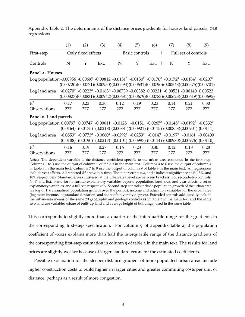
Appendix Table 2: The determinants of the distance prices gradients for houses land parcels, OLS
regressions
(1) (2) (3) (4) (5) (6) (7) (8) (9)
First-step Only fixed effects | Basic controls | Full set of controls
Controls N Y Ext. | N Y Ext. | N Y Ext.
Panel A. HousesLog population -0.00956 -0.00697 -0.00812 -0.0151b -0.0150b -0.0170b -0.0172a -0.0184a -0.0207a
(0.00720)(0.00771)(0.00950)(0.00594)(0.00631)(0.00790)(0.00543)(0.00575)(0.00701)Log land area -0.0270a -0.0223a -0.0163c -0.00739 -0.00382 0.00221 -0.00521 -0.00140 0.00522
(0.00827)(0.00831)(0.00942)(0.00681)(0.00679)(0.00783)(0.00623)(0.00619)(0.00695)
R2 0.17 0.23 0.30 0.12 0.19 0.23 0.14 0.21 0.30Observations 277 277 277 277 277 277 277 277 277
Panel B. Land parcelsLog population 0.00797 0.00747 -0.00611 -0.0128 -0.0151 -0.0265b -0.0148c -0.0192b -0.0332a
(0.0164) (0.0175) (0.0218) (0.00881)(0.00921) (0.0115) (0.00853)(0.00901) (0.0111)Log land area -0.0853a -0.0772a -0.0660a -0.0292a -0.0259a -0.0147 -0.0197b -0.0161 -0.00400
(0.0188) (0.0190) (0.0217) (0.0101) (0.00997) (0.0114) (0.00980)(0.00976) (0.0110)
R2 0.16 0.19 0.27 0.16 0.23 0.30 0.12 0.18 0.28Observations 277 277 277 277 277 277 277 277 277Notes: The dependent variable is the distance coefficient specific to the urban area estimated in the first step.Columns 1 to 3 use the output of column 3 of table 3 in the main text. Columns 4 to 6 use the output of column 4of table 3 in the main text. Columns 7 to 9 use the output of column 9 of table 3 in the main text. All regressionsinclude year effects. All reported R2 are within-time. The superscripts a, b, and c indicate significance at 1%, 5%, and10% respectively. Standard errors clustered at the urban area level are between brackets. For second-step controls,N, Y, and Ext. stand for no further explanatory variables beyond population, land area, and year effects, a set ofexplanatory variables, and a full set, respectively. Second-step controls include population growth of the urban area(as log of 1 + annualised population growth over the period), income and education variables for the urban area(log mean income, log standard deviation, and share of university degrees). Extended controls additionally includethe urban-area means of the same 20 geography and geology controls as in table 3 in the main text and the sametwo land use variables (share of built-up land and average height of buildings) used in the same table.
This corresponds to slightly more than a quarter of the interquartile range for the gradients in
the corresponding first-step specification. For column 9 of appendix table 2, the population
coefficient of -0.021 explains more than half the interquartile range of the distance gradients of
the corresponding first-step estimation in column 9 of table 3 in the main text. The results for land
prices are slightly weaker because of larger standard errors for the estimated coefficients.
Possible explanation for the steeper distance gradient of more populated urban areas include
higher construction costs to build higher in larger cities and greater commuting costs per unit of
distance, perhaps as a result of more congestion.
8

Appendix E. Second-step: spatial heterogeneity
Appendix table 3 duplicates table 4 in the main text and includes interaction terms for population
and income or education. Panel a considers house prices at the centre as dependent variable and
includes the interaction between log city population and log mean city income as explanatory
variable. Panel b also considers house prices as dependent variable and includes the interaction
between log city population and the city share of university graduates as explanatory variable.
Panels c and d mirror the previous two panels but use the land prices instead of house prices as
dependent variable.
Appendix table 4 duplicates table 4 in the main text but it relies on first-step estimates which
also include an interaction term between log distance and log municipal income for which we
estimate a specific coefficient for each urban area. Panel a considers house prices at the centre as
dependent variable while panel b considers unit land prices. For our preferred specification in
column 8, the estimated population elasticity is 0.209 for house prices and 0.592 for land prices,
extremely close to 0.208 and 0.597, respectively, in the corresponding column of table 4 of the main
text. On average, in panel a the coefficients are about 0.03 higher than in the corresponding panel
if table 4. We also note that the more noisy estimates for land prices in panel b. This is likely due
to power issues in the first step as 277 extra coefficients are estimated.
We note finally that a first-step specification including an interaction term between distance
and income group would coincide closely with the predictions of the monocentric urban model
with discrete income groups that differ in size across cities and face different commuting costs
(Duranton and Puga, 2015). Because sorting within cities is in reality less extreme than the perfect
sorting predicted by this simple model and because we have a continuum of incomes instead of
discrete income groups, in our specification we interact continuous income with distance instead
of using indicator variables by income group interacted with distance.
Appendix F. Second-step: all dwellings
The specifications of Appendix table 5 duplicate those of panel a of table 4 in the main text
for housing prices that pertain to all dwellings instead of only houses. We estimate population
elasticities of the price at the centre that are somewhat lower than in table 4 of the main text where
9

Appendix Table 3: The determinants of unit house prices and land values at the centre, OLS
regressions with interactions between population and socioeconomic characteristics
(1) (2) (3) (4) (5) (6) (7) (8) (9)
First-step Only fixed effects | Basic controls | Full set of controls
Controls N Y Ext. | N Y Ext. | N Y Ext.
Panel A. Houses, population and income interactedLog population 0.175a 0.174a 0.223a 0.204a 0.203a 0.288a 0.199a 0.199a 0.291a
(0.0169) (0.0141) (0.0283) (0.0183) (0.0164) (0.0357) (0.0183) (0.0167) (0.0361)Log pop. × log inc. 0.00779a 0.00171 0.000452 0.0102a 0.0102a 0.00816a 0.00993a 0.00816a 0.00624a
(0.00093)(0.00198)(0.00163)(0.000666)(0.00113)(0.00115)(0.00067)(0.00104)(0.00109)Log land area -0.171a -0.152a -0.224a -0.139a -0.118a -0.230a -0.168a -0.149a -0.267a
(0.0174) (0.0136) (0.0293) (0.0205) (0.0182) (0.0364) (0.0193) (0.0168) (0.0375)
R2 0.54 0.65 0.72 0.64 0.69 0.74 0.62 0.67 0.73
Panel B. Houses, population and education interactedLog population 0.171a 0.173a 0.224a 0.205a 0.195a 0.281a 0.200a 0.194a 0.289a
(0.0185) (0.0141) (0.0282) (0.0230) (0.0161) (0.0372) (0.0222) (0.0166) (0.0372)Log pop. × educ. 0.321a 0.195 0.0133 0.374a 1.349a 1.147a 0.365a 0.948a 0.744a
(0.0329) (0.223) (0.184) (0.0465) (0.176) (0.164) (0.0446) (0.196) (0.167)Log land area -0.172a -0.154a -0.224a -0.138a -0.125a -0.233a -0.167a -0.154a -0.271a
(0.0173) (0.0136) (0.0293) (0.0212) (0.0181) (0.0384) (0.0199) (0.0170) (0.0389)R2 0.48 0.65 0.72 0.55 0.70 0.75 0.52 0.68 0.74
Panel C. Land parcels, population and income interactedLog population 0.716a 0.720a 0.908a 0.583a 0.571a 0.653a 0.581a 0.572a 0.704a
(0.0469) (0.0436) (0.120) (0.0354) (0.0328) (0.0841) (0.0350) (0.0337) (0.0861)Log pop. × log inc. 0.00874a -0.00925b -0.0148a 0.0140a 0.0236a 0.0197a 0.0120a 0.0182a 0.0135a
(0.00183)(0.00450)(0.00510) (0.00116) (0.00369)(0.00413)(0.00106)(0.00324)(0.00434)Log land area -0.698a -0.679a -0.906a -0.380a -0.355a -0.472a -0.469a -0.447a -0.608a
(0.0493) (0.0449) (0.131) (0.0402) (0.0368) (0.0906) (0.0399) (0.0367) (0.0936)R2 0.58 0.64 0.70 0.74 0.77 0.80 0.71 0.74 0.78
Panel D. Land parcels, population and education interactedLog population 0.695a 0.718a 0.892a 0.581a 0.572a 0.664a 0.579a 0.577a 0.715a
(0.0472) (0.0423) (0.119) (0.0402) (0.0324) (0.0861) (0.0386) (0.0332) (0.0873)Log pop. × educ. 0.489a -0.655 -0.906b 0.598a 1.868a 1.686a 0.511a 1.228a 1.021a
(0.0757) (0.468) (0.445) (0.0744) (0.338) (0.350) (0.0665) (0.406) (0.382)Log land area -0.703a -0.673a -0.888a -0.378a -0.370a -0.493a -0.467a -0.457a -0.623a
(0.0469) (0.0449) (0.130) (0.0393) (0.0375) (0.0929) (0.0387) (0.0374) (0.0950)R2 0.59 0.64 0.70 0.70 0.77 0.80 0.68 0.74 0.78Notes: 1,937 observations in all columns for panels A and B and 1933 for panels C and D. This table duplicatestable 4 in the main text but also includes an interaction between population and log income or education (share ofuniversity degrees). All reported R2 are within-time. The superscripts a, b, and c indicate significance at 1%, 5%,and 10% respectively. Standard errors clustered at the urban area level are between brackets.
10

Appendix Table 4: The determinants of unit house prices and land values at the centre, OLS
regressions using a first step estimation where distance is interacted with income
(1) (2) (3) (4) (5) (6) (7) (8) (9)
First-step Only fixed effects | Basic controls | Full set of controls
Controls N Y Ext. | N Y Ext. | N Y Ext.
Panel A. HousesLog population 0.262a 0.215a 0.302a 0.258a 0.213a 0.300a 0.253a 0.209a 0.306a
(0.0274) (0.0185) (0.0424) (0.0269) (0.0184) (0.0420) (0.0262) (0.0181) (0.0408)Log land area -0.122a -0.131a -0.245a -0.118a -0.126a -0.241a -0.142a -0.151a -0.276a
(0.0253) (0.0191) (0.0439) (0.0247) (0.0189) (0.0433) (0.0247) (0.0190) (0.0422)
R2 0.44 0.68 0.73 0.44 0.67 0.73 0.40 0.65 0.72Observations 1,937 1,937 1,937 1,937 1,937 1,937 1,937 1,937 1,937
Panel B. Land parcelsLog population 0.869a 0.797a 0.980a 0.649a 0.587a 0.724a 0.650a 0.592a 0.751a
(0.0592) (0.0510) (0.107) (0.0445) (0.0358) (0.0911) (0.0434) (0.0361) (0.0913)Log land area -0.472a -0.489a -0.717a -0.369a -0.382a -0.560a -0.429a -0.440a -0.640a
(0.0603) (0.0548) (0.113) (0.0473) (0.0431) (0.0936) (0.0470) (0.0428) (0.0950)
R2 0.60 0.68 0.71 0.61 0.72 0.77 0.60 0.71 0.76Observations 1,933 1,933 1,933 1,933 1,933 1,933 1,933 1,933 1,933Notes: This table duplicates table 4 of the main text but relies on a first-step estimation that also includes aninteraction term of log distance and log municipal income with a separate coefficient estimated for each urbanarea.
Appendix Table 5: The determinants of unit property prices at the centre, OLS regressions for alldwellings
(1) (2) (3) (4) (5) (6) (7) (8) (9)
First-step Only fixed effects | Basic controls | Full set of controls
Controls N Y Ext. | N Y Ext. | N Y Ext.
Log population 0.200a 0.163a 0.170a 0.222a 0.184a 0.237a 0.182a 0.151a 0.187a
(0.0191) (0.0119) (0.0272) (0.0257) (0.0174) (0.0379) (0.0197) (0.0134) (0.0340)
Log land area -0.129a -0.130a -0.157a -0.0995a -0.104a -0.181a -0.114a -0.117a -0.168a
(0.0198) (0.0125) (0.0287) (0.0227) (0.0176) (0.0367) (0.0184) (0.0140) (0.0351)
R2 0.34 0.66 0.73 0.36 0.61 0.67 0.30 0.57 0.64Observations 1,937 1,937 1,937 1,937 1,937 1,937 1,937 1,937 1,937Notes: The dependent variable is an urban area-time fixed effect estimated in the first step using municipal pricesfor all dwellings instead of only houses. Otherwise, this table is similar to panel A of table 4 in the main text. Thesuperscripts a, b, and c indicate significance at 1%, 5%, and 10% respectively. Standard errors clustered at the urbanarea level are between brackets. All R2 are within time.
11

we consider only houses. This is possibly caused by the lower land intensity of apartments relative
to houses.
To obtain further insight into this question, it is interesting to consider the following back-of-the-
envelop calculation. For our preferred specification of column 8 in appendix table 5, we estimate
an elasticity of the price with respect to population that is about 27% less for all dwellings relatives
to houses, 0.151 instead of 0.208 estimated in the corresponding specification table 4 in the main
text. More generally, in appendix table 5 we estimate population elasticities that are between 10%
and 40% lower for all dwellings relative to the same elasticity for houses only.
Recall that our model interprets the ratio of the elasticity of housing prices to the elasticity of
land prices as the share of land in housing (see Appendix A). Hence, for our preferred estimate
the implicit share of land implied by our model for all dwellings is thus about 0.73 times the share
of land for houses only (and between about 0.6 to 0.9 times when considering all specification of
Appendix table 5 and table 4 of the main text). Put differently, with our preferred specification
we have an implicit share of land for all dwellings of about 0.25 (and more generally between 0.2
and 0.3 for other specifications) instead of 0.35 for houses (which we know from new construction
data).
With about 50% of apartments and 50% of single family homes in French urban areas (cgdd,
2011), this implies a share of land for apartments of 0.15 so that the average between apartments
and houses reaches 0.35 (and more generally we obtain a range between 0.05 and 0.25 for other
specifications regarding the share of land for apartments). While this calculation is subject to
caveats (including applying the share of 0.35 observed in the data for new house constructions
to all houses), these proportions do not strike us as implausible.
Appendix G. Second-step: further robustness checks
Tables 6 and 7 report results for further robustness checks for house prices in panel a and for land
prices in panel b.
The specifications of appendix table 6 experiment with a number of further specifications
regarding the distance gradient using either alternative functional forms to measure distance in
the first step, alternative definitions for centres, richer specifications for distance effects allowing
gradients to vary across years for each urban area, or alternative samples of observations elim-
12

Appendix Table 6: The determinants of unit house prices, further robustness checks part 1
(1) (2) (3) (4) (5) (6) (7)
Panel A. HousesLog population 0.188a 0.228a 0.180a 0.134a 0.207a 0.194a 0.211a
(0.0162) (0.0251) (0.0155) (0.0439) (0.0352) (0.0177) (0.0185)
Log land area -0.149a -0.168a -0.135a -0.0352 -0.140a -0.146a -0.154a
(0.0163) (0.0343) (0.0155) (0.0574) (0.0339) (0.0172) (0.0181)
R2 0.64 0.46 0.61 0.39 0.40 0.64 0.61Observations 1,937 1,937 1,937 1,937 1,937 1,937 1936
Panel B. Land parcelsLog population 0.535a 0.546a 0.542a 0.513a 0.605a 0.620a 0.696a
(0.0317) (0.0433) (0.0332) (0.0512) (0.0400) (0.0348) (0.0937)
Log land area -0.451a -0.486a -0.468a -0.381a -0.389a -0.477a -0.599a
(0.0356) (0.0739) (0.0376) (0.0658) (0.0433) (0.0360) (0.144)
R2 0.70 0.43 0.66 0.57 0.69 0.74 0.20Observations 1,933 1,933 1,933 1,933 1,933 1,933 1,921Notes: a: significant at 1% level; b: significant at 5% level; c: significant at 10% level. Standard errorsclustered at the urban area level are between brackets. All R2 are within time. All OLS regressions. Eachcolumn is a variant of our preferred OLS estimation reported in column 8 of table 4 of the main text. Asexplanatory variables, column 1 includes the distance to the centre of the urban area in level instead ofits log. Column 2 includes log distance and its square (estimating a specific coefficient for each urbanarea for both variables). Column 3 defines the centre of an urban area as the centroid of the municipalitywith the highest residential density. Column 4 measures the distance to the centre as the distance to theclosest of the two municipalities with the highest population in the urban area. Column 5 drops the 25%of observations closest to the centre in each urban area. Column 6 drops the 25% of observations withthe lowest price per square metre in each urban area. Column 7 uses as dependent variable urban-areafixed effects which are estimated allowing for year-specific gradients for each urban area in the first step.
inating potentially more selected observations that are either particularly close to the centre or
particularly cheap.
Recall we mechanically expect a negative correlation between the coefficient on distance, which
measures the price gradient, and the city fixed effect, which measures the intercept. Measuring a
steeper (i.e., more negative) gradient leads mechanically to a higher intercept. For house prices,
the estimated population elasticity is between 0.180 and 0.228 for seven of the eight specifications
of the table instead of 0.208 for our preferred estimate in table 4 of the main text. When allowing
for two centres and measuring the distance to the closest in column 4, the estimated population
elasticity is lower at 0.134. For land prices, we find relatively similar patterns.
Appendix table 7 reports results for specifications that explore two further potential problems.
The first two columns focus on samples of observations that do not contains urban areas with
13

Appendix Table 7: The determinants of unit house prices, further robustness checks part 2
(1) (2) (3) (4) (5) (6) (7) (8)
Panel A. HousesLog population 0.223a 0.214a 0.169a 0.160a 0.208a 0.223a 0.204a 0.186a
(0.0229) (0.0194) (0.0142) (0.0146) (0.006) (0.006) (0.0299) (0.0230)
Log land area -0.168a -0.157a -0.149a -0.0730a -0.152a -0.153a -0.153a -0.147a
(0.0214) (0.0176) (0.0136) (0.0159) (0.007) (0.006) (0.0306) (0.0195)
R2 0.67 0.67 0.59 0.56 0.81 0.78 0.81 0.64Observations 1,546 1,607 1,937 1,937 1,937 1,937 74,621 2,266
Panel B. Land parcelsLog population 0.629a 0.616a 0.523a 0.499a 0.576a 0.664a 0.634a 0.537a
(0.0463) (0.0369) (0.0323) (0.0314) (0.0105) (0.0174) (0.0441) (0.0397)
Log land area -0.478a -0.473a -0.502a -0.479a -0.430a -0.519a -0.493a -0.409a
(0.0479) (0.0382) (0.0343) (0.0334) (0.0116) (0.0195) (0.0513) (0.0328)
R2 0.73 0.73 0.67 0.66 0.73 0.78 0.81 0.68Observations 1,490 1,603 1,933 1,933 1,933 1,933 204,656 2,261Notes: a: significant at 1% level; b: significant at 5% level; c: significant at 10% level. Standard errors clusteredat the urban area level are between brackets (except columns 5 and 6). All R2 are within time. All OLSregressions. Each column is a variant of our preferred OLS estimation reported in column 8 of table 4 ofthe main text. Column 1 drops all urban areas that lost population during the study period. Column 2drops the 20% of urban areas with the lowest growth each year. Column 3 uses as dependent variableurban-area fixed effect which are estimated without weights in the first step. Column 4 uses as dependentvariable urban-area fixed effect which are estimated with population weights in the first step (instead ofusing the number of transactions as weights). Column 5 estimates the regression using feasible generalisedleast squares (FGLS) as described in Appendix H. Column 6 estimates the regression using weighted leastsquares (WLS) as described in Appendix H. Column 7 estimates the elasticity of house prices with respect topopulation in one step instead of two separate steps. Column 8 considers a full sample of 324 urban areasfor which we can estimate our preferred specification instead of our preferred sample of 277.
low or negative growth. As argued by Glaeser and Gyourko (2005), the housing supply curve is
expected to be kinked and much steeper when population declines as the supply of housing is then
inelastic and only adjust following slow depreciation. We either eliminate observations for urban
areas when they experience negative growth during our study period or eliminate every year the
lowest 20% of year-to-year population growth. Overall, eliminating low-growth urban areas leaves
the estimated population elasticity of housing prices unchanged. For land prices, the estimated
population elasticity is marginally higher (albeit statistically undistinguishable). The following
six columns of table 7 experiment with alternative estimation methods that use either a different
weighting scheme in the first-step, a different sample of urban areas, or a different econometric
approach. In particular, recall that our second-step estimation relies on a dependent variable that
is estimated (with error) in a first step. As made clear in appendix Appendix H below, this problem
14

can be addressed using fgls and wls techniques to explicitly account for this sampling error. We
can also estimate the population elasticity of prices at the centre in a single step. Finally, we also
estimate the population elasticity on a larger sample of urban areas (324 instead of 277).
We estimate smaller population elasticities by up to 0.05 smaller than our preferred elasticity of
table 4 in the main text for both house and land prices when using alternative weighting schemes.
We also estimate a slightly smaller elasticity when using a larger sample of urban areas, for which
the added urban areas are mostly small. This is consistent with the possibility entertained below
that this elasticity may be smaller for smaller urban areas. For our other variants, the results only
differ marginally.
Appendix H. Second-step: FGLS and WLS estimators
In this appendix, we explain how we construct weighted least squares (wls) and feasible general
least squares (fgls) estimators used in some second-stage regressions of the previous appendix.
The model is of the form:
C = Xϕ + ζ + η , (h1)
where C is a JT× 1 vector stacking the estimated urban area-time fixed effects capturing unit house
or land prices at the centre, ln CP or ln CR, with J the number of urban areas, X is a JT × K matrix
stacking the observations for urban area variables (area, population, population growth, etc.), ζ
is a JT × 1 vector of error terms supposed to be independently and identically distributed with
variance σ2, and η is a JT × 1 vector of sampling errors with known covariance matrix V.
It is possible to construct a consistent fgls estimator of ϕ as:
ϕFGLS =(
X′Ω−1X)−1
X′Ω−1C , (h2)
where Ω is a consistent estimator of the covariance matrix of ζ + η, Ω = σ2 I + V. To compute this
estimator, we use an unbiased and consistent estimator of σ2 which can be computed from the ols
residuals of equation (h1) denoted ζ + η:
σ2 =1
N − K
[ζ + η
′ζ + η − tr (MXV)
], (h3)
where MX = I − X (X′X)−1 X′ is the projection orthogonally to X. We thus use Ω = σ2 I + V in
the computation of (h2). A consistent estimator of the covariance matrix of the fgls estimator is:
V (ϕFGLS) =(
X′Ω−1X)−1
. (h4)
15

As the fgls is said not to be always robust, we also compute a wls estimator in line with
Card and Krueger (1992), using the diagonal matrix of inverse of first-stage variances as weights,
denoted ∆. The estimator is given by:
ϕWLS =(X′∆X
)−1 X′∆C , (h5)
with a consistent estimator of the covariance matrix given by:
V (ϕWLS) =(X′∆X
)−1 X′∆Ωw∆X(X′∆X
)−1 ,
where Ωw = σ2w I + V with σ2
w a consistent estimator of σ2 based on the residuals of wls denoted
∆1/2 (ζ + η) and given by:
σ2w =
1tr (∆1/2M∆1/2X∆1/2)
[∆1/2 (ζ + η)
′ ∆1/2 (ζ + η)− tr(
∆1/2M∆1/2X∆1/2V)]
. (h6)
Appendix I. Second-step: IV results
The key identification worry when estimating the elasticity of prices with respect to population
equations (7) or (8) in the main text is the endogeneity of population either because of some
missing variable(s) that is correlated with both prices at the centre and population or because of
reverse causation. The high correlation between population and land area implies that land area
is also potentially endogenous. Both sources of endogeneity can be addressed with instrumental
variables. As described in the main text, we consider two sets of instruments, either amenity
variables or long historical lags.
The rationale for using amenities as instruments follows the logic of the model where amenities
attract population to an urban area without otherwise affecting the demand or supply for housing.
The use of long lags for population, area, or density is motivated by the idea that the factors that
made an urban area a particularly cheap (or expensive) place to live nearly two centuries ago differ
from the factors that drive the demand or supply of housing today.3
While we can easily test for the strength of these instruments, the exclusion restrictions as-
sociated with our instruments require further discussion. First, as mentioned in the text the
correlations between our instruments are low. January temperatures are poorly correlated with
other instruments. Among historical variables, the correlations between population lags and
3As mentioned in the main text, there is a long tradition that uses long historical lags as instruments for urbanarea population when estimating agglomeration effects following Ciccone and Hall (1996) or Combes, Duranton, andGobillon (2008). The literature is reviewed in Combes and Gobillon (2015).
16

area lags are also low. Getting the same results from different sources of variation in the data is
reassuring. Second, we can introduce controls to our instrumental regressions to preclude possible
correlations between our instruments and the error term. We can introduce these controls either at
the first stage or at the second stage. A possible issue with introducing more controls is that these
controls may themselves be endogenous and correlated with city population. Below, we report
results for different combinations of instruments and different specifications that include fewer or
more controls.
The four panels of appendix table 8 report results for a series of iv regressions that house prices
as dependent variable. The specifications of panel a include the same set of control variables as
our preferred ols regressions while those of panel b do not include second-step controls beyond
those for which we report coefficients and time indicators. Panels c and d duplicate the first two
panels but consider a dependent variable estimated without first-stage controls. We first note that
historical instruments are in general strong whereas amenities tend to be weaker even though they
pass weak instrument requirements. Interestingly, including controls or controls appears to matter
little for the strength of the instruments. Consistent with their relative strength, the standard errors
on the estimated coefficients are smaller when using historical instruments rather than amenities.
We made the choice of using exactly the same sets of instruments for all panels to allow for more
meaningful comparisons of points estimates between panels.
Turning to the analysis of the coefficients, in panel a where controls are included in both steps,
the population elasticity of prices remains between 0.215 and 0.267. These elasticities range from
marginally above our preferred ols estimate to about 25% larger. With the higher iv coefficients
being less precisely identified, these differences between iv and ols are not statistically significant.
We nonetheless keep in mind this variation in the point estimates when computing the urban
cost elasticity in section 7 of the main text. As for the slight increase in the size of the estimated
population elasticity, we can only speculate about what might drive it. Although we think this is
unlikely, our instruments may correct for measurement error. A more plausible explanation to us
may be that our ols estimates may suffer from a minor reverse causation bias where urban areas
with higher urban costs may end up with a smaller population. Another possible explanation may
be that our instruments have more bite for larger cities for which the population elasticity may be
larger as shown in the next appendix.
17

Appendix Table 8: The determinants of unit house prices at the centre, IV estimations
(1) (2) (3) (4) (5) (6) (7) (8)
Panel A. Log house prices per m2, with first-step and second-step controls
Log population 0.247a 0.225a 0.250a 0.226a 0.227a 0.267a 0.215a 0.266a
(0.0358) (0.0249) (0.0281) (0.0248) (0.0249) (0.0557) (0.0226) (0.0563)Log land area -0.170a -0.141a -0.175a -0.140a -0.142a -0.217a -0.150a -0.216a
(0.0411) (0.0205) (0.0238) (0.0204) (0.0203) (0.0677) (0.0213) (0.0684)
First-stage statistic 34.5 130.1 84.2 119.1 120.1 9.3 101.3 6.2Overidentification p-value . 0.41 0.88 0.95 0.20 . 0.29 0.79
Panel B. Log house prices per m2, with first-step controls and without second-step controls
Log population 0.237a 0.211a 0.245a 0.211a 0.214a 0.392a 0.237a 0.400a
(0.0494) (0.0353) (0.0393) (0.0351) (0.0351) (0.0759) (0.0302) (0.0768)Log land area -0.119b -0.0859a -0.130a -0.0858a -0.0891a -0.276a -0.0789b -0.287a
(0.0555) (0.0308) (0.0337) (0.0308) (0.0305) (0.0927) (0.0334) (0.0941)
First-stage statistic 32.2 139.7 99.9 122.8 129.2 9.9 155.0 7.1Overidentification p-value . 0.53 0.83 0.60 0.05 . 0.02 0.72
Panel C. Log house prices per m2, without first-step controls and with second-step controls
Log population 0.204a 0.188a 0.207a 0.188a 0.189a 0.243a 0.187a 0.249a
(0.0295) (0.0185) (0.0217) (0.0187) (0.0187) (0.0498) (0.0164) (0.0608)Log land area -0.170a -0.148a -0.175a -0.147a -0.149a -0.223a -0.151a -0.231a
(0.0337) (0.0148) (0.0174) (0.0148) (0.0146) (0.0610) (0.0158) (0.0753)
First-stage statistic 34.5 130.1 84.2 119.1 120.1 9.3 101.3 6.2Overidentification p-value . 0.44 0.86 0.15 0.18 . 0.21 0.12Panel D. Log house prices per m2, without first-step and second-step controls
Log population 0.194a 0.174a 0.203a 0.173a 0.177a 0.353a 0.205a 0.420a
(0.0450) (0.0256) (0.0290) (0.0259) (0.0255) (0.0687) (0.0230) (0.0949)Log land area -0.126b -0.100a -0.138a -0.0994a -0.103a -0.280a -0.0905a -0.364a
(0.0514) (0.0253) (0.0271) (0.0255) (0.0250) (0.0854) (0.0280) (0.119)
First-stage statistic 32.2 139.7 99.9 122.8 129.2 9.9 155.0 7.1Overidentification p-value . 0.60 0.79 0.08 0.05 . 0.02 0.13InstrumentsUrban population in 1831 Y Y Y Y Y N N NUrban pop. density in 1851 Y Y Y N N N N NUrban area in 1851 N N Y N N N N NUrban pop. density in 1881 N Y N Y Y N Y NJanuary temperature N N N Y N N N YNumber of hotel rooms N N N N N Y Y YShare of one-star hotel rooms N N N N Y Y Y YObservations 1,937 1,937 1,937 1,937 1,937 1,937 1,937 1,937Notes: a: significant at 1% level; b: significant at 5% level; c: significant at 10% level. Standard errors are clustered at the urban arealevel. The first-step controls are the same as in column 9 of table 3 of the main text. The second-step controls correspond to thecontrols used in columns 2, 5, and 8 of table 4 of the main text. All estimations are performed with LIML. The critical value for 10%maximal LIML size of Stock and Yogo (2005) weak identification test is 7.03 for columns (1) and (6) and 5.44 for other columns.They do not depend on control variables because the role of those is first conditioned out before the estimation. This conditioningdoes not affect the estimates and their standard error for population and area but it is required due to multicolinearity arisingfrom a few urban areas with too few observations. The first-stage statistics is the Kleibergen-Paap rk Wald F.
18

The estimates of the population elasticity of prices reported in panels b to d are very close to
those of panel a. The main exceptions are the much higher elasticities estimated when using only
amenities. These higher amenities are nonetheless imprecisely estimated so that it is hard to draw
conclusions from these results.
Appendix table 9 duplicates appendix table 8 for land prices instead of house prices. In par-
ticular, we use the instruments in all panels as for house prices. In substance, the results are very
similar. The presence or absence of first or second step controls makes only modest differences
to the strength of the instruments and the estimated coefficients. The specifications that use only
amenities are more fragile and often estimate sizeably higher coefficients for population. With
historical instruments, the estimated population elasticities are modestly above our preferred ols
estimate.
Appendix J. Second-step: non-constant elasticity
Appendix table 10 duplicates some ols specifications of table 4 in the main text as well as some iv
specifications in the same spirit as those of tables 8 and 9 above and includes terms of higher order
for population, namely the square and cube of log population. Panel a considers house prices at
the centre as dependent variable while panel b uses land prices.
We find that when estimating specifications with only a quadratic term, the coefficient of this
term is generally positive and significant. This is suggestive of a convex relationship between log
prices for houses or land and log population. As a caveat, we note that this convexity is driven by
the three or four largest French urban areas. When we estimate specifications with both a quadratic
and a cubic term for log populations, the coefficients are generally not significant.
Adding a quadratic term for log population to our preferred specification of column 8 of table 4
in the main text implies an elasticity of house prices with respect to population of 0.205 for an urban
area with 100,000 inhabitants, an elasticity of 0.288 for an urban area with a million inhabitants,
and 0.378 for an urban area with the same population as Paris. Because, the non-linear estimate of
the population elasticity for Paris is nearly twice as large as our preferred ols estimate of 0.208, we
keep this range in mind for our computation of the urban cost elasticity in section 7 of the main
text.
19

Appendix Table 9: The determinants of unit land prices at the centre, IV estimations
(1) (2) (3) (4) (5) (6) (7) (8)
Panel A. Log land prices per m2, with first-step and second-step controls
Log population 0.684a 0.641a 0.696a 0.650a 0.647a 0.776a 0.627a 0.920a
(0.0799) (0.0508) (0.0580) (0.0522) (0.0512) (0.125) (0.0467) (0.264)Log land area -0.507a -0.451a -0.524a -0.453a -0.455a -0.661a -0.469a -0.845b
(0.0891) (0.0461) (0.0513) (0.0467) (0.0457) (0.157) (0.0477) (0.336)
First-stage statistic 32.5 120.2 79.4 110.8 111.2 9.7 76.3 6.5Overidentification p-value . 0.43 0.80 0.00 0.11 . 0.17 0.03
Panel B. Log land prices per m2, with first-step controls and without second-step controls
Log population 0.676a 0.620a 0.692a 0.621a 0.625a 0.905a 0.651a 0.888a
(0.0880) (0.0577) (0.0649) (0.0575) (0.0574) (0.155) (0.0510) (0.175)Log land area -0.439a -0.368a -0.462a -0.366a -0.373a -0.687a -0.363a -0.664a
(0.0999) (0.0543) (0.0590) (0.0546) (0.0539) (0.194) (0.0564) (0.220)
First-stage statistic 31.2 134.0 97.6 118.3 121.5 8.8 150.1 6.2Overidentification p-value . 0.42 0.79 0.31 0.09 . 0.06 0.21
Panel C. Log land prices per m2, without first-step controls and with second-step controls
Log population 0.729a 0.711a 0.744a 0.716a 0.713a 0.752a 0.719a 0.781a
(0.0994) (0.0577) (0.0665) (0.0594) (0.0583) (0.150) (0.0533) (0.273)Log land area -0.690a -0.667a -0.711a -0.668a -0.667a -0.707a -0.664a -0.744b
(0.114) (0.0546) (0.0605) (0.0549) (0.0537) (0.186) (0.0566) (0.346)
First-stage statistic 32.5 120.2 79.4 110.8 111.2 9.7 76.3 6.5Overidentification p-value . 0.80 0.82 0.01 0.85 . 0.82 0.01Panel D. Log land prices per m2, without first-step and second-step controls
Log population 0.729a 0.695a 0.751a 0.696a 0.697a 0.843a 0.738a 0.832a
(0.111) (0.0579) (0.0656) (0.0584) (0.0578) (0.175) (0.0564) (0.177)Log land area -0.629a -0.586a -0.659a -0.586a -0.588a -0.702a -0.568a -0.687a
(0.130) (0.0642) (0.0687) (0.0643) (0.0632) (0.221) (0.0662) (0.223)
First-stage statistic 31.2 134.0 97.6 118.3 121.5 8.8 150.1 6.2Overidentification p-value . 0.70 0.77 0.87 0.77 . 0.54 0.76InstrumentsUrban population in 1831 Y Y Y Y Y N N NUrban pop. density in 1851 Y Y Y N N N N NUrban area in 1851 N N Y N N N N NUrban pop. density in 1881 N Y N Y Y N Y NJanuary temperature N N N Y N N N YNumber of hotel rooms N N N N N Y Y YShare of one-star hotel rooms N N N N Y Y Y YObservations 1,933 1,933 1,933 1,933 1,933 1,933 1,933 1,933
Notes: a: significant at 1% level; b: significant at 5% level; c: significant at 10% level. Standard errors are clustered at the urban arealevel. The first-step controls are the same as in column 9 of table 3 of the main text. The second-step controls correspond to thecontrols used in columns 2, 5, and 8 of table 4 of the main text. All estimations are performed with LIML. The critical value for 10%maximal LIML size of Stock and Yogo (2005) weak identification test is 7.03 for columns (1) and (6) and 5.44 for other columns.They do not depend on control variables because the role of those is first conditioned out before the estimation. This conditioningdoes not affect the estimates and their standard error for population and area but it is required due to multicolinearity issuesarising from a few urban areas with too few observations. The first-stage statistics is the Kleibergen-Paap rk Wald F.
20
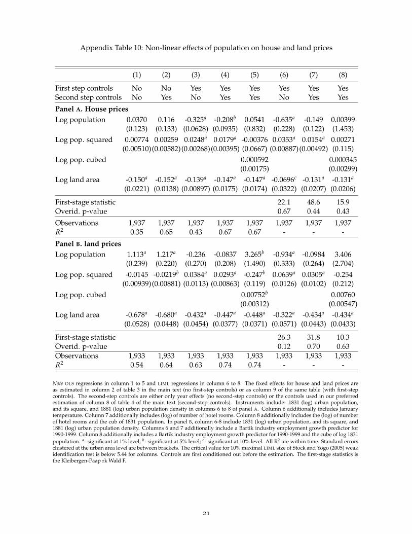
Appendix Table 10: Non-linear effects of population on house and land prices
(1) (2) (3) (4) (5) (6) (7) (8)
First step controls No No Yes Yes Yes Yes Yes YesSecond step controls No Yes No Yes Yes No Yes Yes
Panel A. House pricesLog population 0.0370 0.116 -0.325a -0.208b 0.0541 -0.635a -0.149 0.00399
(0.123) (0.133) (0.0628) (0.0935) (0.832) (0.228) (0.122) (1.453)Log pop. squared 0.00774 0.00259 0.0248a 0.0179a -0.00376 0.0353a 0.0154a 0.00271
(0.00510)(0.00582)(0.00268)(0.00395) (0.0667) (0.00887)(0.00492) (0.115)Log pop. cubed 0.000592 0.000345
(0.00175) (0.00299)Log land area -0.150a -0.152a -0.139a -0.147a -0.147a -0.0696c -0.131a -0.131a
(0.0221) (0.0138) (0.00897) (0.0175) (0.0174) (0.0322) (0.0207) (0.0206)
First-stage statistic 22.1 48.6 15.9Overid. p-value 0.67 0.44 0.43
Observations 1,937 1,937 1,937 1,937 1,937 1,937 1,937 1,937R2 0.35 0.65 0.43 0.67 0.67 - - -
Panel B. land pricesLog population 1.113a 1.217a -0.236 -0.0837 3.265b -0.934a -0.0984 3.406
(0.239) (0.220) (0.270) (0.208) (1.490) (0.333) (0.264) (2.704)Log pop. squared -0.0145 -0.0219b 0.0384a 0.0293a -0.247b 0.0639a 0.0305a -0.254
(0.00939)(0.00881) (0.0113) (0.00863) (0.119) (0.0126) (0.0102) (0.212)Log pop. cubed 0.00752b 0.00760
(0.00312) (0.00547)Log land area -0.678a -0.680a -0.432a -0.447a -0.448a -0.322a -0.434a -0.434a
(0.0528) (0.0448) (0.0454) (0.0377) (0.0371) (0.0571) (0.0443) (0.0433)
First-stage statistic 26.3 31.8 10.3Overid. p-value 0.12 0.70 0.63Observations 1,933 1,933 1,933 1,933 1,933 1,933 1,933 1,933R2 0.54 0.64 0.63 0.74 0.74 - - -
Note OLS regressions in column 1 to 5 and LIML regressions in column 6 to 8. The fixed effects for house and land prices areas estimated in column 2 of table 3 in the main text (no first-step controls) or as column 9 of the same table (with first-stepcontrols). The second-step controls are either only year effects (no second-step controls) or the controls used in our preferredestimation of column 8 of table 4 of the main text (second-step controls). Instruments include: 1831 (log) urban population,and its square, and 1881 (log) urban population density in columns 6 to 8 of panel A. Column 6 additionally includes Januarytemperature. Column 7 additionally includes (log) of number of hotel rooms. Column 8 additionally includes the (log) of numberof hotel rooms and the cub of 1831 population. In panel B, column 6-8 include 1831 (log) urban population, and its square, and1881 (log) urban population density. Columns 6 and 7 additionally include a Bartik industry employment growth predictor for1990-1999. Column 8 additionally includes a Bartik industry employment growth predictor for 1990-1999 and the cube of log 1831population. a: significant at 1% level; b: significant at 5% level; c: significant at 10% level. All R2 are within time. Standard errorsclustered at the urban area level are between brackets. The critical value for 10% maximal LIML size of Stock and Yogo (2005) weakidentification test is below 5.44 for columns. Controls are first conditioned out before the estimation. The first-stage statistics isthe Kleibergen-Paap rk Wald F.
21

Appendix Table 11: The determinants of unit house prices and land values at the centre, OLS
regressions without land area
(1) (2) (3) (4) (5) (6) (7) (8) (9)
First-step Only fixed effects | Basic controls | Full set of controls
Controls N Y Ext. | N Y Ext. | N Y Ext.
Panel A. HousesLog population 0.110a 0.0775a 0.0234b 0.178a 0.136a 0.0883a 0.151a 0.109a 0.0561a
(0.0110) (0.0103) (0.00936) (0.0178) (0.0128) (0.0139) (0.0157) (0.0122) (0.0124)R2 0.24 0.53 0.67 0.40 0.62 0.69 0.33 0.58 0.67Observations 1,937 1,937 1,937 1,937 1,937 1,937 1,937 1,937 1,937
Panel B. Land parcelsLog population 0.296a 0.262a 0.0671b 0.434a 0.365a 0.242a 0.352a 0.299a 0.163a
(0.0252) (0.0348) (0.0303) (0.0288) (0.0252) (0.0271) (0.0262) (0.0265) (0.0256)R2 0.23 0.34 0.59 0.54 0.66 0.75 0.44 0.55 0.70Observations 1,933 1,933 1,933 1,933 1,933 1,933 1,933 1,933 1,933Notes: This table duplicates table 4 in the main text but omits land area as an explanatory variable.
Appendix K. Second-step results without land area
Appendix table 11 duplicates table 4 in the main text but omits land area as an explanatory
variable. What is estimated here is the population elasticity of house and land prices when we
allow for land area to adjust to population growth.
In appendix table 11, we find that for both house and land prices, the coefficient on population
is smaller than when land area is included and typically larger than (or about equal to) the sum
of the coefficients on population and land in table 4 in the main text. This is consistent with the
standard prediction of land use models for monocentric cities: When cities grow in population,
they physically expand slightly less than proportionately and become denser (Duranton and Puga,
2015). When we regress log area on log population, we estimate a coefficient of about 0.7, consistent
with our comparison between appendix table 11 and table 4 in the main text.
The other remarkable result of appendix table 11 is that the population elasticity of land prices is
about three times as large as the population elasticity of house prices. This occurs despite sizeable
fluctuations in the absolute value of these elasticities across specifications. This result is highly
consistent with our theoretical model which predicts that the ratio of these two elasticities should
be equal to the inverse of the share of land in the value of houses. This share is equal to 0.36 in our
22

Appendix Table 12: The determinants of house prices at the centre, IV estimations in difference
(1) (2) (3) (4)
First-step controls Yes No Yes NoSecond-step controls No No Yes Yes
Log population 0.917a 0.929b 1.932b 1.993b
(0.338) (0.363) (0.813) (0.893)
First-stage statistic 16.3 16.3 7.5 7.5Overidentification p-value 0.09 0.10 0.91 0.88
InstrumentsNumber of hotel rooms Y Y N NUrban population in 1831 Y Y N NBartik industry 1999-2011 Y Y Y YBartik occupation 2006-2011 Y Y Y YObservations 275 275 275 275
Notes: a: significant at 1% level; b: significant at 5% level; c: significant at 10% level. White-robust standard errors. The first-stepcontrols are the same as in column 9 of table 3 in the main text. The second-step controls correspond to the extended controlsused in column 8 of table 4 that are time varying. All estimations are performed with limited information maximum likelihood(LIML). The critical value for 10% maximal LIML size of Stock and Yogo (2005) weak identification test is 5.44 in columns (1) and(2) and 8.68 in all columns (3) and (4). For these columns, it is 5.33 for 15% maximal LIML size. The first-stage statistics is the theKleibergen-Paap rk Wald F.
data for the new constructions associated with the land parcels that we observe.
Appendix L. Second-step: IV estimations for 2000-2012 differences
When regressing 2012-2000 changes in house prices at the centre on changes in population over
the same period, the latter is potentially endogenous. An unobserved labour demand shock in an
urban area may simultaneously determine house price growth and population growth. It is also
possible that house price growth affects population growth. To address this worry, we follow a
standard strategy initially proposed by Bartik (1991) and often used in subsequent literature (e.g.,
Diamond, 2016, among many others).
The idea of the ‘Bartik instrument’ is that we can predict the population growth of cities us-
ing their initial structure of sectoral employment interacted with the national growth of sectoral
employment. Loosely put, a city with a high fraction of employment in high-end services in
2000 is expected to enjoy more growth from 2000 to 2012 than a city with a high initial share of
employment in traditional manufacturing which kept declining over the period. We also develop
a parallel approach using the initial structure of employment by occupations and national changes
23
in employment by occupation. This approach is described in greater details in Appendix B.
The results are reported in appendix table 12. While the results do not contradict those of table
5 in the main text, the point estimates are noisy, in particular when we include changes in income,
education, and inequality as controls in columns 3 and 4. These imprecise estimates are probably
the consequence of our instruments being marginally weak for these specifications. This is perhaps
unsurprising. Changes in labour demand may be tracked by changes in predicted employment
(our instrument) but also by changes in local incomes (a control). Put differently, our controls may
condition out much of the variation contained in the Bartik predictors. The estimates of columns
1 and 2, which do not include changes in income, education, and inequality for the urban area
as controls lead to stronger instruments and relatively more precisely estimated coefficients. The
point estimates are also more in line with those obtained without instrumenting in table 5 of the
main text.
Appendix M. The share of housing in expenditure: supplementary results
In addition to the issues already discussed in the main text, we may also worry that our results
for the joint sample of homeowners and renters may mask some important heterogeneity between
the two groups. To gain insight into this issue, we duplicate the results of table 6 in the main text
separately for homeowners and renters in the two panels of appendix table 13. We first note that,
unsurprisingly, renters are more prevalent than homeowners in larger urban areas. The difference
is nonetheless modest as mean urban area population is 3.13 million for homeowners instead of
3.29 million for renters. A comparison of the two samples of renters and homeowners also indicates
that renters devote a slightly larger share of their income to housing than homeowners.4
Turning to the coefficients on city population, we find that they are very close for renters
and homeowners in most ols specifications. Modest differences arise when we instrument for
population. We then estimate coefficients of 0.055 for homeowners and 0.034 for renters instead
of 0.048 for the pooled sample of column 8 of table 6 of the main text. While the coefficients
on population for renters and homeowners differ, they remain less than two standard deviations
4This difference remains somewhat modest at about 4 percentage points after we account for the difference in meancity population. This difference even flips signs if we also account for income differences across both groups. Overall,these results suggest small differences between the two groups.
24

Appendix Table 13: The share of housing in expenditure for homeowners and private renters
(1) (2) (3) (4) (5) (6) (7) (8)Panel A. HomeownersLog population 0.027a 0.029a 0.041a 0.045a 0.044a 0.055a 0.076a 0.055a
(0.001) (0.002) (0.005) (0.008) (0.008) (0.014) (0.013) (0.012)Log land area -0.020 -0.028a -0.033a -0.038a -0.057a -0.038a
(0.007) (0.008) (0.007) (0.013) (0.012) (0.011)Population growth 2.593b 2.662a 2.443a 2.470a 2.084a 2.471a
(0.610) (0.727) (0.743) (0.763) (0.780) (0.740)Log distance to city centre -0.005 -0.004 -0.006c -0.002 -0.008b -0.013a -0.008b
(0.005) (0.005) (0.003) (0.003) (0.004) (0.004) (0.003)Log income -0.252a -0.253a -0.253a -0.256a -0.168a -0.256a -0.257a -0.256a
(0.012) (0.011) (0.011) (0.010) (0.013) (0.009) (0.009) (0.009)
First-stage statistic 253.2 97.0 5.8 14.9Overidentification p-value 0.33 0.26 0.05InstrumentsDegree XUrban population in 1831 X XConsumption amenities X XLocal controls No No No Yes Yes Yes Yes YesR2 0.53 0.53 0.54 0.55Panel B. RentersLog population 0.030a 0.033a 0.038a 0.028a 0.021a 0.028c 0.056a 0.034a
(0.002) (0.002) (0.009) (0.009) (0.008) (0.014) (0.017) (0.012)Log land area -0.008 0.005 0.009 0.005 -0.021 -0.001
(0.013) (0.012) (0.011) (0.018) (0.019) (0.016)Population growth 2.775b 3.950a 4.205a 3.957a 3.277b 3.806a
(1.262) (1.116) (1.184) (1.256) (1.273) (1.217)Log distance to city centre -0.009b -0.009b -0.005 -0.003 -0.005 -0.011b -0.006
(0.004) (0.004) (0.005) (0.005) (0.005) (0.006) (0.005)Log income -0.342a -0.342a -0.341a -0.343a -0.184a -0.343a -0.343a -0.343a
(0.023) (0.023) (0.023) (0.022) (0.033) (0.022) (0.022) (0.022)
First-stage statistic 31.6 157.4 8.1 22.0Overidentification p-value 0.03 0.03 0.01R2 0.58 0.58 0.58 0.59
Notes: a: significant at 1% level; b: significant at 5% level; c: significant at 10% level. All R2 are within time. The same regressionsare estimated in both panels. 5,984 observations in each regression of panel A corresponding to 177 urban areas. 2,464 observationsin each regression of panel B corresponding to 177 urban areas (20 of which differ from the previous sample). All variables arecentred and the estimated constant, which corresponds to the expenditure share in a city of average size (2.94 million inhabitantsin panel A and 3.12 million in panel B), takes the value 0.314 in all specifications of panel A and 0.352 in all specifications of panelB. Regressions are weighted with sampling weights and include: age and dummies for year 2011 (ref. 2006), living in couplewithin the dwelling (ref. single), one child, two children, three children and more (ref. no child). Standard errors are clusteredat the urban area level. Local controls include the same geography variables for urban areas as in table 4 of the main text andthe same geology, land use, and amenity variables as in table 3 of the main text. OLS for columns (1) to (4). IV estimated withlimited information maximum likelihood (LIML) in columns (5) (income instrumented), (6) and (7) (population instrumented)and (8) (income and population instrumented). The first-stage statistics is the Kleibergen-Paap rk Wald F. The critical value for10% maximal LIML size of Stock and Yogo (2005) weak identification test is 4.45 for column (5), 16.38 for column (6), 3.50 forcolumn (7), and 3.42 for column (8). The instruments are the same as in table 8. The education instruments are five indicatorvariables corresponding to PhD and elite institution degree,master, lower university degree, high school and technical degree,lower technical degree, and primary school (reference).
25

Appendix Figure 1: Share of housing in household expenditure and log city population
0.0
0.2
0.4
0.6
8 10 12 14 16
Log population
Housing expenditure share
Notes: The horizontal axis represents log urban area population. The vertical axis represents the urban area median ofthe residual of column 8 of table 6 in the main text plus log urban area population multiplied by its estimated coefficient.The plain continuous curve is a quadratic trend line. The dotted line is a linear trend.
apart. They are also, for most of them, in the same range as our estimates for the pooled sample in
table 6 of the main text.
In results not reported here, we also experimented with instrumenting for land area using 1881
population density in addition to population. This does not affect our results in any major way.
For instance, we estimate a coefficient on city population of 0.039 for city population instead of
0.048 in column 8 of table 6 of the main text when also instrumenting for land area. We also
experimented with including education directly as a control variable to condition out elements
of permanent income instead of instrumenting. This does not affect the coefficient on urban area
population. Using education as a control variable to the specification of column 4 of table 6 of the
main text leads to a coefficient 0.033 for population instead of 0.036 in column 5 where it is used as
instrument.
Our last worry is about functional forms. Our (semi log) linear estimation of a share of expen-
diture on a log population we fail to capture important non-linearities as population increases. In
figure 1, we provide a ‘component plus residual’ plot where we represent the share of housing in
expenditure after controlling for other controls on the vertical axis and log urban area population
on the horizontal axis. The figure also contains two trend lines, linear and quadratic. As made
clear by the figure, the two trends are virtually undistinguishable except for the very top of the
26

Appendix Table 14: The elasticity of urban costs
City 1 (pop. 100,000) City 2 (pop. 1m) City 3 (pop. Paris)
Panel A. Population elasticity of prices
Baseline (preferred OLS) 0.208 0.208 0.208 0.208 0.208 0.208 0.208 0.208 0.208Non-linear population elasticity 0.205 0.205 0.205 0.288 0.288 0.288 0.378 0.378 0.37812-year adjustment 0.780 0.780 0.780 0.780 0.780 0.780 0.780 0.780 0.780Allowing for urban expansion 0.109 0.109 0.109 0.109 0.109 0.109 0.109 0.109 0.109
Panel B. Housing share
Slope of the housing share 0.028 0.048 0.067 0.028 0.048 0.067 0.028 0.048 0.067Share of housing in expenditure 0.093 0.159 0.228 0.247 0.269 0.293 0.363 0.390 0.415
Panel C. Urban costs elasticity using:
Baseline 0.019 0.033 0.048 0.051 0.056 0.061 0.075 0.081 0.086(0.007) (0.007) (0.005) (0.005) (0.005) (0.005) (0.007) (0.007) (0.008)
Non-linear population elasticity 0.019 0.032 0.047 0.071 0.078 0.084 0.137 0.147 0.157(0.002) (0.007) (0.005) (0.007) (0.007) (0.007) (0.015) (0.017) (0.018)
12-year adjustment 0.073 0.124 0.178 0.193 0.210 0.228 0.283 0.304 0.324(0.031) (0.036) (0.041) (0.044) (0.047) (0.051) (0.063) (0.069) (0.073)
Allowing for urban expansion 0.010 0.017 0.025 0.027 0.029 0.032 0.040 0.043 0.045(0.004) (0.004) (0.003) (0.003) (0.003) (0.004) (0.004) (0.005) (0.005)
Notes: In panel A, row 1, the estimate of 0.208 is our preferred OLS estimate from column 8 of table 4. In row 2, the three estimatesare marginal effects computed from column 4 of appendix table 10. In row 3, the estimate of 0.780 is for the 2000-2012 differencefrom column 8 of table 5. In row 4, we use the elasticity of 0.109 estimated in column 8 of appendix table 11, which does not includeland area as a control. In panel B, for the coefficient on log population for the housing share we report our preferred estimate fromcolumn 8 of table 6 as well as the largest and smallest coefficients for log population estimated in the same table. From thesecoefficients and the constant of the regression, we compute the predicted housing share in expenditure for our three hypotheticalcities. Panel C reports the urban cost elasticity for all the combinations of housing share in expenditure and population elasticityof house prices. Standard errors in brackets computed from the estimated coefficients and their variances using the followingformula for the variance of their product: var(XY) = var(X)var(Y) + var(X)E(Y)2 + var(Y)E(X)2.
distribution. For a city of the size of Paris, the difference between the linear and quadratic trends is
a modest 2 percentage points. For a city of the size of Lyon (the second largest city), the difference
is already less than half of a percentage point. Consistent with this, the difference in explanatory
power between the quadratic and linear trends is small. We have an R2 of 63.1% for the quadratic
instead of 62.8% for the linear trend line. Hence, we conclude that our log linear specification
provides an accurate first-order description of the relationship between housing expenditure and
city population, except for Paris that deviates modestly.
27

Appendix N. More complete results for the urban cost elasticity
While in the main text, we focus on the share of housing in expenditure predicted from our pre-
ferred estimate for the coefficient on log city population of 0.048 in table 6 of the main text, in this
appendix we also consider a lower estimate of 0.028 and a higher estimate of 0.067 corresponding
to the lowest and highest estimated coefficients for log city population obtained in table 6 of the
main text. The predicted share of housing in expenditure for the three cities associated with the
three scenarios described above are reported in panel b of appendix table 14. We note that for a city
like Paris or for a city with a million inhabitants, the predicted share of housing in expenditure is
only modestly affected by the value that we consider for the population semi elasticity. Differences
are larger for a city with 100,000 inhabitants.
Consistent with this result, we find that the exact way we predict the share of housing in expen-
diture only makes a modest difference to our estimated urban cost elasticity for the hypothetical
cities with one or 12 million inhabitants like Paris. Appendix table 14 reports a full set of results.
The differences are more sizeable for a smaller city with 100,000 inhabitants. For this hypothetical
city, we prefer to rely on the predicted share of housing in expenditure of 0.159 coming from our
preferred estimate of 0.048 for log population. This share of 0.159 is close to the share we observe in
the data for actual urban areas of this size. Our more extreme values for the population coefficient
predict housing shares of 0.228 or 0.093, which are out of line with the raw data.
28

References
Bartik, Timothy. 1991. Who Benefits from State and Local Economic Development Policies? Kalamazoo(mi): W.E. Upjohn Institute for Employment Research.
Card, David and Alan B. Krueger. 1992. School quality and black-white relative earnings: A directassessment. Quarterly Journal of Economics 107(1):151–200.
Ciccone, Antonio and Robert E. Hall. 1996. Productivity and the density of economic activity.American Economic Review 86(1):54–70.
Combes, Pierre-Philippe, Gilles Duranton, and Laurent Gobillon. 2008. Spatial wage disparities:Sorting matters! Journal of Urban Economics 63(2):723–742.
Combes, Pierre-Philippe, Gilles Duranton, Laurent Gobillon, and Sébastien Roux. 2010. Estimatingagglomeration economies with history, geology, and worker effects. In Edward L. Glaeser (ed.)The Economics of Agglomeration. Cambridge (ma): National Bureau of Economic Research, 15–65.
Combes, Pierre-Philippe and Laurent Gobillon. 2015. The empirics of agglomeration economies. InGilles Duranton, Vernon Henderson, and William Strange (eds.) Handbook of Regional and UrbanEconomics, volume 5A. Amsterdam: Elsevier, 247–348.
Commissariat Général au Développement Durable. 2011. Comptes du Logement: Premiers Résultats2010, le Compte 2009. Paris: Ministère de l’Ecologie, du Développement Durable, des Transportset du Logement.
Diamond, Rebecca. 2016. The determinants and welfare implications of US workers’ diverginglocation choices by skill: 1980-2000. American Economic Review 106(3):479–524.
Duranton, Gilles and Diego Puga. 2015. Urban land use. In Gilles Duranton, J. Vernon Henderson,and William C. Strange (eds.) Handbook of Regional and Urban Economics, volume 5A. Amsterdam:North-Holland, 467–560.
Glaeser, Edward L. and Joseph Gyourko. 2005. Urban decline and durable housing. Journal ofPolitical Economy 113(2):345–375.
Guérin-Pace, France and Denise Pumain. 1990. 150 ans de croissance urbaine. Economie et Statis-tiques 0(230):5–16.
Stock, James H. and Motohiro Yogo. 2005. Testing for weak instruments in linear IV regression.In Donald W.K. Andrews and James H. Stock (eds.) Identification and Inference for EconometricModels: Essays in Honor of Thomas Rothenberg. Cambridge: Cambridge University Press, 80–108.
29