University of Southampton Research Repository
ePrints Soton
Copyright © and Moral Rights for this thesis are retained by the author and/or other copyright owners. A copy can be downloaded for personal non-commercial research or study, without prior permission or charge. This thesis cannot be reproduced or quoted extensively from without first obtaining permission in writing from the copyright holder/s. The content must not be changed in any way or sold commercially in any format or medium without the formal permission of the copyright holders.
When referring to this work, full bibliographic details including the author, title, awarding institution and date of the thesis must be given e.g.
AUTHOR (year of submission) "Full thesis title", University of Southampton, name of the University School or Department, PhD Thesis, pagination
http://eprints.soton.ac.uk

UNIVERSITY OF SOUTHAMPTON
Faculty of Engineering, Science and Mathematics
Institute of Sound and Vibration Research
THE CALCULATION OF NOISE FROM RAILWAY
BRIDGES AND VIADUCTS
BY
OLIVER GUY BEWES
Thesis submitted for the degree of Engineering Doctorate
September 2005

i
UNIVERSITY OF SOUTHAMPTON
ABSTRACT
FACULTY OF ENGINEERING, SCIENCE AND MATHEMATICS
INSTITUTE OF SOUND AND VIBRATION RESEARCH
Engineering Doctorate
THE CALCULATION OF NOISE FROM RAILWAY BRIDGES AND
VIADUCTS
By
Oliver Guy Bewes
Pandrol Rail Fastenings Limited are a designer and manufacturer of railway rail-fastening
systems. As an organisation they have the capability to reduce the noise impact of bridges
using resilient track components. They also have a commercial interest in providing such
technology. Knowledge of the processes behind bridge noise is important to Pandrol in two
ways; to aid the engineers within the organisation in the design of fastening systems and to
demonstrate a state-of-the-art understanding of the problem of railway bridge noise to
customers, as this will aid in the sale of Pandrol products.
The fitting of new rail components to an existing track form, or failure to meet noise
regulations with a new track form, can be costly. It is important to be able to predict
accurately the effectiveness of noise reduction techniques. Currently, Pandrol’s knowledge
of the problem consists almost entirely of experience gained and data gathered while
working on existing bridge projects.
To expand their knowledge base, Pandrol perform noise and vibration measurements on
railway bridges and viaducts and then use the measured data to predict the performance of
their systems on other bridges. This completely empirical approach to predicting bridge
noise is both costly and situation specific results cannot be provided before the installation
of the fastening system.

ii
Another approach to predicting bridge noise is through the application of analytical
models. Limited analytical modelling in the context of bridge noise is currently conducted
within the organisation. For these reasons, Pandrol are sponsoring research into bridge
noise in the form of this EngD project.
Here an existing rapid calculation approach is identified that relies less on the exact
geometry of the bridge and more on its general characteristics. In this approach an
analytical model of the track is coupled to a statistical energy analysis (SEA) model of the
bridge. This approach forms a suitable basis from which to develop a better model here by
concentrating on its weaknesses.
A mid-frequency calculation for the power input to the bridge via a resilient track system
has been developed by modelling the track-bridge system as two finite Timoshenko beams
continuously connected by a resilient layer. This has resulted in a power input calculation
which includes the important effects of coupling between the rail and bridge and the
resonance effects of the finite length of a bridge.
In addition, a detailed study of the frequency characteristics of deep I-section beams has
been performed using Finite Element, Boundary Element and Dynamic stiffness models. It
is shown that, at high frequencies, the behaviour of the beam is characterised by in-plane
motion of the beam web and bending motion in the flange. This knowledge has resulted in
an improved calculation for the mobility of a bridge at high frequencies.
The above improvements are included in an improved model for use by Pandrol in their
general activities. Data from real bridges is compared to predictions from the improved
model in order to validate different aspects of the model. The model is then used to study
the effect on noise of varying many bridge design parameters. It is shown that the
parameter that has most influence on the noise performance of a bridge is the dynamic
stiffness of the resilient rail fastening system. Additionally it is demonstrated that for a
given bridge and noise receiver location, an optimum fastener stiffness exists where the
noise radiated by the bridge and track is at a minimum.

iii
ACKNOWLEDGEMENT
Firstly I would like to thank my supervisors at the ISVR, Dr Chris Jones and Prof. David
Thompson for their supervision, instruction and support during this project. I would also
like to thank Pandrol Rail Fastenings for sponsoring this project and my industrial
supervisors, Dr Anbin Wang, Steve Cox, and Dr Chris Morison for their valued support.
Additionally I must thank Serco Docklands Limited (London), MTR Corporation (Hong
Kong) and Banverket (Sweden) for granting permission to publish data obtained on their
railways in this work.

iv
CONTENTS
ACKNOWLEDGEMENT................................................................................................ III
CONTENTS....................................................................................................................... IV
LIST OF SYMBOLS ........................................................................................................ IX
1. INTRODUCTION....................................................................................................1
1.1. RAILWAY NOISE IN THE CONTEXT OF INDUSTRY ...................................1
1.2. NOISE LEGISLATION AND RAIL SYSTEMS..................................................2
1.3. NOISE FROM RAILWAY BRIDGES AND VIADUCTS...................................3
1.4. RESILIENT TRACK SUPPORT COMPONENTS ..............................................4
1.4.1. Ballasted track................................................................................................5
1.4.2. Directly fastened track ...................................................................................7
1.4.3. Floating slab track FST ..................................................................................9
1.5. FASTENER STIFFNESS ....................................................................................10
1.5.1. Static stiffness ..............................................................................................10
1.5.2. Dynamic stiffness.........................................................................................11
1.5.3. Goals when selecting fastener stiffness........................................................11
1.6. LITERATURE REVIEW.....................................................................................12
1.6.1. Empirical literature.......................................................................................12
1.6.2. Developments of track/bridge models .........................................................17
1.6.3. Bridge noise calculation models ..................................................................18
1.7. APPROACHES TO THE CALCULATION OF BRIDGE NOISE - NORBERT ..
..............................................................................................................................21
1.7.1. Roughness excitation ...................................................................................22
1.7.2. Rail/wheel interaction ..................................................................................23
1.7.3. Track model .................................................................................................23
1.7.4. Rolling stock model .....................................................................................24
1.7.5. Power input to the bridge .............................................................................24
1.7.6. Input mobility of bridge deck.......................................................................25
1.7.7. Vibration transmission throughout the bridge .............................................27
1.7.8. Sound power radiated by the bridge ............................................................27

v
1.7.9. Wheel and track noise ..................................................................................28
1.8. SUMMARY AND OBJECTIVES OF THESIS ..................................................28
1.9. PROJECT PROGRAMME ..................................................................................31
2. MODEL FOR A RAIL RESILIENTLY MOUNTED ON A BRIDGE ............32
2.1. TWO INFINITE BEAMS CONNECTED BY A RESILIENT LAYER.............33
2.1.1. Equations of motion .....................................................................................33
2.1.2. Response to a point force. ............................................................................34
2.1.3. Equivalent point stiffness.............................................................................35
2.2. TWO INFINITE EULER BEAMS CONNECTED BY A RIGID MASS LAYER
AND TWO RESILIENT LAYERS .................................................................................36
2.2.1. Equations of motion .....................................................................................37
2.3. TWO FINITE EULER BEAMS CONNECTED VIA A RESILIENT LAYER .38
2.3.1. Response to a point force. ............................................................................39
2.4. TWO FINITE TIMOSHENKO BEAMS CONNECTED BY A RESILIENT
LAYER ............................................................................................................................40
2.4.1. Equations of motion .....................................................................................40
2.4.2. Response to a point force .............................................................................41
2.5. POWER DISTRIBUTION..................................................................................43
2.5.1. Power input to bridge ...................................................................................43
2.5.2. Power dissipated in resilient layer................................................................44
2.5.3. Power dissipated in the rail ..........................................................................45
2.6. RESULTS ............................................................................................................45
2.6.1. Infinite cases.................................................................................................46
2.6.2. Finite cases ...................................................................................................50
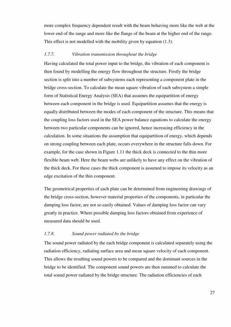
2.6.3. Timoshenko beam cases...............................................................................52
2.7. SUMMARY .........................................................................................................54
3. THE MOBILITY OF A BEAM............................................................................56
3.1. FINITE ELEMENT MODEL OF RECTANGULAR SECTION BEAMS.........57
3.1.1. FE results......................................................................................................58
3.1.2. Effect of position on driving point mobility ................................................60
3.1.3. Effect of varying length and depth...............................................................60
3.1.4. Effect of varying thickness...........................................................................62

vi
3.1.5. Effect of varying damping ...........................................................................62
3.2. BEAMS WITH A FLANGE................................................................................63
3.2.1. Beam representation of a flange...................................................................64
3.2.2. Shell representation of flange.......................................................................66
3.3. A SIMPLE MODEL FOR THE DRIVING POINT MOBILITY AT LOW
FREQUENCIES...............................................................................................................69
3.3.1. Infinite beam models....................................................................................69
3.3.2. Finite beam model........................................................................................70
3.4. MODEL FOR THE TRANSITIONAL BEHAVIOUR RANGE ........................71
3.5. MODEL FOR THE MOBILITY AT HIGH FREQUENCY ...............................74
3.5.1. Boundary element model .............................................................................76
3.5.2. Boundary element results.............................................................................78
3.5.3. Calibration of in-plane plate equation..........................................................80
3.6. MODEL FOR THE DRIVING POINT MOBILITY OF AN I-SECTION BEAM.
..............................................................................................................................83
3.6.1. Motivation....................................................................................................83
3.6.2. Rod with equal masses at each end ..............................................................84
3.6.3. Rod with equal apparent mass at each end...................................................86
3.6.4. Coupled beam and rod model. .....................................................................88
3.6.5. Calculation of the transitional mode ............................................................91
3.7. EXPERIMENTS ON WROUGHT IRON I-SECTION BEAM ..........................92
3.7.1. Measurement method ...................................................................................93
3.7.2. Measurement results and discussion. ...........................................................93
3.8. SUMMARY .........................................................................................................95
4. ON TRACK MEASUREMENTS.........................................................................96
4.1. INTRODUCTION ...............................................................................................96
4.2. MEASUREMENT METHOD .............................................................................96
4.3. STEEL-CONCRETE COMPOSITE VIADUCT ON DLR.................................98
4.3.1. Measurement method ...................................................................................99
4.3.2. Modelling ...................................................................................................101
4.3.3. Results and model validation. ....................................................................105
4.4. MEASUREMENTS ON A CONCRETE VIADUCT IN HONG KONG.........111
4.4.1. Measurement Method.................................................................................114

vii
4.4.2. Modelling ...................................................................................................115
4.4.3. Results and model validation. ....................................................................116
4.5. MEASUREMENTS ON A STEEL RAILWAY BRIDGE IN SWEDEN.........128
4.5.1. Measurement method .................................................................................130
4.5.2. Modelling ...................................................................................................130
4.5.3. Results and model validation .....................................................................132
4.6. SUMMARY .......................................................................................................134
5. THE EFFECT ON NOISE OF VARYING CERTAIN BRIDGE DESIGN
PARAMETERS................................................................................................................137
5.1. INTRODUCTON...............................................................................................137
5.1.1. Purpose of parameter study........................................................................137
5.1.2. Parameters that affect the noise radiated by a bridge.................................137
5.2. THE BRIDGES..................................................................................................138
5.2.1. All-concrete viaduct. ..................................................................................138
5.2.2. Steel-concrete composite viaduct...............................................................139
5.2.3. All-steel steel bridge ..................................................................................140
5.3. THE TRACK AND ROLLING STOCK ...........................................................141
5.4. EFFECT OF BRIDGE STRUCTURE ON NOISE RADIATED......................143
5.4.1. The power input to the bridge structure .....................................................147
5.4.2. Sound radiation from the bridge structure .................................................151
5.4.3. Effect of varying structural damping .........................................................155
5.4.4. Effect of varying plate thickness................................................................159
5.5. EFFECT OF THE TRACK ON TOTAL SOUND POWER RADIATED........162
5.5.1. Effect of varying fastener stiffness ............................................................162
5.5.2. The importance of receiver position with respect to a noise barrier. .........169
5.5.3. Effect of varying input excitation ..............................................................171
5.5.4. Effect of varying train speed ......................................................................173
5.6. SUMMARY .......................................................................................................176
6. SUMMARY OF CONCLUSIONS AND RECOMMENDATIONS FOR
FUTURE WORK .............................................................................................................177
6.1. MODEL OF A RAIL RESILIENTLY SUPPORTED ON A BRIDGE ............178
6.2. THE MOBILITY OF A BEAM.........................................................................178

viii
6.3. ON TRACK MEASUREMENTS......................................................................179
6.4. THE EFFECT ON NOISE OF VARYING CERTAIN BRIDGE DESIGN
PARAMETERS .............................................................................................................181
6.5. RECOMMENDATIONS FOR FUTURE WORK ............................................182
6.6. BENEFIT TO PANDROL .................................................................................183
7. REFERENCES.....................................................................................................184
APPENDIX A. PARAMETERS USED TO DEFINE THE ROLLING STOCK
AND VIADUCT ON DLR...............................................................................................189
APPENDIX B. PARAMETERS USED TO DEFINE THE ROLLING STOCK
AND VIADUCT ON AEL HONG KONG.....................................................................191
APPENDIX C. PARAMETERS USED TO DEFINE THE ROLLING STOCK
AND ARSTA BRIDGE....................................................................................................193

ix
LIST OF SYMBOLS
A cross-sectional area m2
An amplitude of travelling wave
a excitation radius m
B bending stiffness Nm2
B(η) damping correction factor
b depth/width of beam m
c0 speed of sound in air ms-1
cB bending wave speed ms-1
cl longitudinal wave speed ms-1
cR Rayleigh wave speed ms-1
cs shear wave speed ms-1
E Young’s modulus of elasticity Nm-2
F force N
f frequency Hz
fn natural frequency Hz
G shear modulus Nm-2
H transfer function
h thickness of beam or plate m
I second moment of area m4
K dynamic stiffness Nm-1
k wavenumber
L, l length m
M, mass, bending moment kg, Nm
m mass kg
Neq number of equivalent independent excitations
P power W
S surface area, shear force m2, N
s dynamic stiffness per unit length Nm-2
u, v, w flexural displacement m

x
un, vn eigenvectors of waves in source beam and receiver beams
V velocity ms-1
v vibration velocity ms-1
W moment mobility ms-1N-1
Y mobility ms-1N-1
Z impedance mN-1
β complex wavenumber
η hysteretic loss factor
φ angle of rotation
κ Timoshenko shear coefficient
λ wavelength m
λn eigenvalues
µ mass per unit length (beam or plate) kgm-1
ν Poisson’s ratio
ρ density kgm-3
ρ0 density of air kgm-3
σ radiation efficiency
θ shear angle, bending rotation
ω circular frequency rads-1
ζ damping ratio
spatially-averaged response

1
1. INTRODUCTION
1.1. RAILWAY NOISE IN THE CONTEXT OF INDUSTRY
Pandrol Rail Fastenings Limited are a designer and manufacturer of railway rail-fastening
systems. They produce rail clips and a range of baseplates and fastener designs. As an
organisation they have the capability to reduce the noise impact of bridges using resilient
track components. They also have a commercial interest in providing such technology.
Knowledge and understanding of the processes behind bridge noise is important to Pandrol
in two ways:
1. To aid the engineers within the organisation in the design of fastening systems.
2. To demonstrate a state-of-the-art understanding of the problem of railway bridge noise
externally to customers, as this will aid in the sale of Pandrol products.
As the fitting of new rail components to an existing track form, or failure to meet noise
regulations with a new track form, can be costly, it is important to be able to predict
accurately the effectiveness of noise reduction techniques. Currently, Pandrol’s knowledge
and understanding of the problem consists almost entirely of experience gained and data
gathered while working on existing bridge projects.
To expand their knowledge base, Pandrol perform noise and vibration measurements on
railway bridges and viaducts. Ideally, to add maximum value to the organisation, these
measurements are performed before and after the installation of a Pandrol fastening
system. This will allow the effectiveness of the fastening system to be fully evaluated.
Complete noise surveys on railways are expensive and it is rare that Pandrol will be paid
by a customer to perform them. Furthermore, a detailed survey on a viaduct will require
full access to the track while no trains are running. Due to strict time and safety constraints,
surveys can also be expensive to conduct for the railway operating company. In many
cases it is not cost effective or permission is not granted to conduct a full survey.
Another limitation of a completely empirical approach to predicting bridge noise is that
situation specific results cannot be provided before the installation of the fastening system.
This is acceptable when designing a system for a bridge that is similar to those that Pandrol
have worked with previously. However in some cases, Pandrol are presented with a bridge

2
design of which they have limited knowledge. In this situation the effectiveness of the
fastening system is more difficult to predict.
Another approach to predicting bridge noise is through the application of analytical
models. Proper application of a bridge noise model will allow the assessment of the
effectiveness of Pandrol products without performing costly noise surveys on bridges.
Furthermore, if chosen correctly, a model can be used to predict the noise of novel bridge
and track designs. Limited analytical modelling in the context of bridge noise is currently
conducted within the organisation. For these reasons, Pandrol have sponsored research into
the calculation of bridge noise in the form of this EngD project.
The aim of this project, described in more detail below, is therefore to develop a rapid
bridge noise modelling approach, which can be used as a tool for Pandrol to aid the design
of fastening systems and can be used to demonstrate a state-of-the-art understanding of
bridge noise issues.
1.2. NOISE LEGISLATION AND RAIL SYSTEMS
Increasing demand for the movement of people and freight is resulting in an increasingly
congested transport infrastructure in the western world. Heightened pressures on the
environment in terms of pollution of the areas in which people live go hand in hand with
this. Noise is an important aspect of the pollution of our living space. As a fall in demand
for travel is unlikely, governments are keen to encourage the use of environmentally
friendly methods of transport. Railway transport is generally seen as a safer, less polluting
mode of transport than road or air transport in most categories of impact. However, noise is
seen as one of its main weaknesses.
Environmental noise of all forms is also increasingly being viewed as a problem that needs
addressing. Many governments are currently setting out legislation that regulates the
assessment and management of environmental noise. For example the Environmental
Noise Directive or END (European parliament, 2002), sets out the policy on noise from
industry, road traffic, air traffic and railways in all European Union countries. The
directive requires competent authorities in EU Member States to produce strategic noise
maps around main transport infrastructures and in major agglomerations, to inform the
public about noise exposure and its effects, and to draw up action plans to reduce noise
where necessary and maintain environmental noise quality where it is good. Action plans

3
are to be drawn up by 2007 and brought into place by 2008. It has led to legislation in a
number of member states, such as the Swiss “Noise emission limitation of rolling stock”
(Bundesamt für Verkehr (Schweiz), 1994), which places limits on noise from railways
systems.
As yet, no END action plans are in place in the UK and little national railway specific
noise legislation exists. For most new railway projects, noise limits are set in negotiation
between the project owners and the relevant local authorities and or parliament. Following
public enquiry a set of undertakings are developed which can be very specific, for
example, a finite maximum noise level may be set at a defined property along the
alignment of the new railway system. The undertakings are enforceable and if not adhered
to by the project contractors, they will be in breach of contract.
Although not directly limiting noise from UK railways systems, Railway Noise and
Insulation of Dwellings (Department of Transport, 1991) sets day and night time noise
limits at properties surrounding new railway systems, above which the railway operator
has a duty to insulate the property against the noise of the railway.
Such regulation means that there is a great need for manufacturers, engineers and designers
to understand the mechanisms behind railway noise in order to be able to reduce it at the
source where possible.
1.3. NOISE FROM RAILWAY BRIDGES AND VIADUCTS.
Bridges are commonplace in the world’s transport infrastructure, whenever there is a need
for transport to cross rivers, roads and valleys etc. Furthermore, due to the combination of
road and rail traffic that exists in urban environments, many bridges can be found in
heavily populated residential or commercial areas. There is clearly a need to understand the
processes behind bridge noise in order to be able to put measures in place to mitigate such
noise, where appropriate.
For railway systems in general, the predominant source of noise is rolling noise (Jones &
Thompson, 2003), which is the broadband noise caused by the vibrations of the wheels,
sleepers and rails. When a train passes over a bridge there is an increase in the rolling noise
due to the vibration response of the bridge that represents a large radiating surface area.

4
The measured noise levels when a train passes over a bridge are usually greater than those
measured when a train passes over normal track; up to 10 dB higher (Janssens &
Thompson, 1996). Figure 1.1 shows a flow diagram of the process (based on (Janssens &
Thompson, 1996)) that leads to this increase in noise as a train passes over a bridge.
Small irregularities, usually referred to as roughness, exist on the surface of wheels and
rails in all railway systems (Remington, 1976) which, due to wheel/rail interaction, cause
the rail to vibrate during the pass-by of a train. The vibration is then transmitted through
the track fastenings and input to the bridge structure, unlike plain track where the energy is
absorbed in the ground. The energy is then transmitted throughout the various structural
components of the bridge, causing them to vibrate and hence radiate sound.
Figure 1.1. A flow diagram representing the processes behind bridge noise.
1.4. RESILIENT TRACK SUPPORT COMPONENTS
Figure 1.1 above showed the processes that lead to train pass-by noise being radiated by a
bridge structure. The second element in the flow diagram represents the power flow from
the rail through the track fastening system and into the bridge structure. Although an over-
simplification of the problem, a rail mounted on a massive structure via a resilient
fastening system can be modelled as a linear, one-dimensional, purely translational mass-
spring system as presented in Beranek and Vér, 1992. According to this theory, isolation of
the bridge structure from the vibrating rail is only achieved at frequencies greater
than nf2 , where nf is the natural frequency of the rail/wheel mass vibrating on the
Rail Vibration
Power Input To Bridge
Energy Flow in Structu r e
Total Sound power radiated
wheel/rail roughness

5
resilient fastening system. Therefore for good isolation of the bridge from the vibrating rail
and wheel, an isolator with the lowest possible fn is required. To achieve this, the stiffness
of the fastening system must be as low as possible or the vibrating mass must be as high as
possible. In practical terms it is often undesirable to add a large mass to a system.
Therefore, in most cases vibration isolation problems are addressed by reducing the
stiffness of the resilient fastening components.
The above example is an over-simplification of the problem, but highlights the fact that the
resilience of rail fastening systems is the primary design parameter for Pandrol in order to
manufacture products that are effective at achieving good isolation. Below a short review
of the most common types of resilient track support systems is given for clarity and for
reference later in this thesis.
1.4.1. Ballasted track
Figure 1.2 shows a schematic of a ballasted track form. Typically a 0.2 to 0.3 m layer of
coarse-grain crushed granite rock lies over the ground along the length of the track. Timber
or concrete sleepers are laid on the layer of granite perpendicular to the track direction at
equally spaced intervals, usually less than one metre apart. This can be seen more clearly
in Figure 1.3, an example of a ballasted track form on the Arad bridge in Romania. The
primary function of the sleepers is to provide support for the rail foot and a fixing location
for the rail fasteners that maintains the distance between the rails. The rail foot is fixed to
the sleepers using a rail fastening system such a baseplate. A resilient rail pad is usually
placed between the sleeper and rail as part of the fastening system.
Ballasted track forms are the most common type of track systems used worldwide. They
are generally the most resilient of track types (Esveld, 1989) with most of the resilience
coming from the layer of crushed granite that acts like a spring between the sleeper and
track bed. The dynamic stiffness of a ballast layer has strongly frequency dependent
characteristics due to the relatively thick layer used and the high mass of the ballast
(Thompson & Jones, 2002).

6
If a ballasted track form is to be used on a bridge, the rail pad or system that fastens the rail
to the sleeper can be replaced by a softer1 system to add more resilience to the track form
(Pandrol Rail Fastenings, 2002). However, unless the pad is much softer than the ballast
layer the effect is negligible and the use of soft rail pads in this situation is usually to
reduce the wear on the sleepers and ballast layer that comes from the dynamic force of the
train passing over the track (Grassie, 1989). Alternatively, extra resilience can be obtained
by laying a ballast mat between the ballast bed and the track bed.
rail
rail pad sleeper
ballast layer ballast mat
Figure 1.2. A schematic of a ballasted track form with sleepers.
1 In the railway industry the term ‘soft’ is more commonly used than ‘resilient’ to describe an isolating track
fastening system.

7
Figure 1.3. An example of a ballasted track form on Arad Bridge in Romania.
1.4.2. Directly fastened track
In a directly fastened track form, no sleepers or layers of ballast are present. The rail is
directly fastened to a concrete track bed or steel bridge deck with a baseplate system.
Directly fastened track forms are used as alternatives to ballasted track when the addition
of a large mass of sleepers and ballast is undesirable, such as on bridges, or when there is
little space for a track form or regular maintenance must be eliminated, such as in tunnels
(Esveld, 1989). Figure 1.4 shows an example of a rail directly fastened to a concrete track
bed using the Pandrol Vanguard baseplate system.
Since no resilient ballast layer is present, all of the resilience in the system must be present
at the connection to the track bed. Therefore to be effective in isolation, the support must
be very soft. Typical dynamic stiffness values of the pads in direct fastening systems range
from 4 MN/m to 100 MN/m as opposed to a value of 100 MN/m to 5000 MN/m that would
typically be found in the fastener to the sleeper in normal track.

8
Figure 1.4. An example of a directly fastened track form in Hong Kong.
Figure 1.5 shows the Pandrol Vanguard direct fastening system. The rail is supported at its
head by two rubber wedges, which give the system its resilience. The Vanguard fastening
system is a novel design and contrasts with most direct fastening systems where the
resilience comes from a traditional pad supporting the rail at its foot.
Figure 1.6 shows a diagram of the Pandrol VIPA fastening system. This is an example of a
double-layer baseplate system. The rail is supported by a rail pad on a top plate. A second
layer of resilience is provided with a pad between the top plate and subplate. In terms of
vibration isolation, the extra layer of resilience provides increased isolation with increasing
frequency in the isolation range (Beranek and Vér, 1992).

9
Figure 1.5. A drawing of the Pandrol VANGUARD direct fastening system.
Figure 1.6. A diagram of the Pandrol VIPA fastening system.
1.4.3. Floating slab track FST
Figure 1.7 shows a diagram of a floating slab track form (FST). The construction is similar
to that of a directly fastened track as the rail is fastened to the concrete track bed using
baseplates. However, in an FST system extra resilience is added by laying the slab on a
resilient mat or helical springs. The principle is similar to that of a double layer baseplate.
Also the large mass of the slab, together with the extra resilience of the slab support, means
that the decoupling frequency of the system from the track bed is typically less than 20 Hz,
the lowest of all the track forms mentioned here. An FST form is usually used in favour of
a ballasted track form in situations when there is little space available to perform regular
maintenance, such as in a tunnel.

10
rail
rail pad
concrete slab
resilient mat, pads or helical springs
Figure 1.7. A schematic of a floating slab track form.
1.5. FASTENER STIFFNESS
In simple terms the stiffness of a ‘spring’ system is defined as the ratio of the load to the
resulting deflection in the spring. The ‘spring’ element in a resilient fastening system is
most commonly an elastomeric material such as a cork-rubber rail pad. The stiffness of this
element can be defined as its static stiffness or its dynamic stiffness. These stiffnesses are
related to one another, but each is important for a different aspect of track design.
1.5.1. Static stiffness
Figure 1.8 shows a typical load-deflection curve for an elastomeric rail pad. Under static
loading, elastomers have a non-linear load-deflection curve. In general the stiffness of an
elastomer increases with increasing load. This means that the static stiffness of a resilient
rail fastening must be defined at a particular load. This load will depend on factors such as
axle load of the expected traffic.
Also shown in Figure 1.8 are two definitions of the static stiffness of a fastener, tangent
stiffness and secant stiffness. The secant stiffness is measured as the static stiffness
between the clip load and a stated wheel load. For small deflections about a mean load, the
tangent stiffness is more appropriate. Thus for vibrational loading, this is the appropriate
definition.

11
Figure 1.8. A typical load-deflection curve for an elastomeric rail pad.
1.5.2. Dynamic stiffness
Under static loading an elastomer normally acts as a Hookean elastic spring, where the
deflected shape will return to its original shape when the load is removed. When the
material is subject to stresses and strains that change with time, such as the excitation due
to wheel-rail roughness, the material exhibits viscoelastic behaviour.
The viscoelastic nature of elastomer fastenings produces lower deflections under dynamic
loads compared to static loads, meaning that the dynamic stiffness is much higher than the
static stiffness. The deflection also lags the applied load due to the damping effect. The
dynamic stiffness is the more important parameter in terms of vibration attenuation.
1.5.3. Goals when selecting fastener stiffness
When selecting the ideal static and dynamic stiffness of a fastening the following three
factors, in order of importance, are (TCRP, 2005):
1. Minimizing the wheel impacts on the track supports (safety criteria).
2. Constraining the rail from excessive motion particularly gauge widening and
vertical deflection (safety criteria).

12
3. Providing the correct level of vibration isolation from the rail and the support
structure.
The force acting on the track sub-structure due to the wheel impacts can be reduced by
reducing the static stiffness of the resilient fastening system (Grassie, 1989), more
specifically the vertical stiffness of the fastener. It was also described in Section 1.4 that
higher levels of vibration isolation of the rail from the support structure are achieved by
using a resilient fastening with a low vertical dynamic stiffness. Therefore, with regards to
the stiffness of the fastening system, factors 1 and 3 are in affinity with one another.
Excessive vertical motion in the rail will lead to excessive bending stress in the rail foot.
This will reduce the fatigue life of the rail and lead to rail breaks. The vertical motion of
the rail can be constrained by increasing the static stiffness of the resilient fastening
system. Excessive lateral motion or rail roll will lead to gauge widening. This will
adversely affect the steering dynamics at track-bogie interaction and in extreme cases can
lead to derailment. As for the vertical motion, the lateral motion of the rail can be
constrained by increasing the lateral stiffness of the fastening system. For a standard
resilient baseplate fastening system the vertical and lateral stiffness are dependent on each
other. A vertically ‘soft’ fastening system will inherently have a low lateral stiffness.
Thus, in terms of selecting the correct stiffness of the resilient fastening system, factor 2
opposes factors 1 and 3. Therefore a balance between excessive motion of the rail and
sufficient attenuation of impacts or vibration is required when selecting the correct fastener
stiffness. This is why, in noise and vibration problems, there is a lower limit to the vertical
dynamic stiffness of the fastening system that can be used. This depends on the specific
application.
Standards and legislation which define the best practices
1.6. LITERATURE REVIEW
1.6.1. Empirical literature
Stüber (1963) investigated the differences in noise level measured when an electric
locomotive travelled at 80 km/h over two identical steel railway bridges, one with ballasted
track and one with the track fastened directly to the deck of the bridge (direct fastening).
The paper reports an improvement of 13 dB (A) when ballasted track was used rather than

13
direct fastening. However the bridge studied had a very high mobility so the improvement
is likely to be due to factors other than isolation. This was investigated further by Stüber
(1975), by placing a layer of sand over the bridge deck before taking noise measurements.
Improvements of 7 dB (B) were seen in the noise level below the bridge. This showed that
the improvements seen in (Stüber, 1963) were more likely to be due to increased mass and
damping of the bridge deck.
As well as conducting similar exercises to Stüber’s, measurements were performed on
many other types of bridge in ORE (1966), ORE (1969) and ORE (1971). This was the
beginning of attempts to categorise bridge types with reference to the noise produced by
each bridge.
Japanese National Railways (1975) performed experiments to investigate the effect of
using ballast mats on bridges. An improvement of 8 dB (A) was seen in the wayside noise
levels for a steel bridge deck. Ban and Miyamoto (1975), also investigated the effect of
using a ballast mat on a concrete viaduct. An improvement of 7 dB (A) below the viaduct
was reported. However the results were considered unreliable between 250 Hz and 1 kHz.
Kurzweil (1977) used measurements from (ORE, 1971) and (Japanese National Railways,
1975) and divided the bridges studied into eleven categories according to construction
materials, geometry and fastening system. As each measurement was taken with different
train speeds and lengths passing over the bridges, Kurzweil applied a simple correction for
this, which allowed each bridge type to be directly compared with each other in terms of
overall noise level.
Ungar and Wittig (1980) added more measurements and then separated them into main and
sub categories according to the criteria shown in Figure 1.9. The measurements were then
presented relative to the same train on plain track. Figure 1.9 shows an adapted version of
the diagram presenting ranges of noise level increase for different bridge types seen in
(Ungar and Wittig, 1980). It is clear from the measurements gathered in (Ungar and Wittig,
1980) that steel bridges are generally noisier than concrete bridges and direct fastening
systems are noisier than ballasted track, with a few exceptions. Ungar and Wittig (1980)
provide a good method to gauge how noisy a particular bridge may be, although it is by no
means a comprehensive model that accounts for all possible noise generating effects.

14
Structure type & authority
Noise increase (dBA)
-5 0 5 10 15
Concrete deck/structure, with ballast.
DB.
JNR.
SNCF.
Concrete deck on steel structure, with ballast.
JNR.
SNCF.
CFF.
Steel deck on steel structure, with ballast.
DB.
Concrete deck/structure without ballast.
RM.
NS.
Concrete deck on steel structure, without ballast.
JNR.
SNCF.
DB.
Open Tie deck on steel beams.
JNR.
SNCF.
DB.
CFF.
NS.
Steel deck on steel structure, without ballast.
SH.
DB.
NS.
SNCF.
Legend:
= Track on top of structure.
= Track in trough formed by beams.
= Box beam, track on top.
= Lattice or truss beams.
= Rail bearers.
= Configuration not specified.
JNR = Japanese National Railway
DB = German State Railway
CFF = Swiss Railways
SNCF = French National Railway
NS = Netherlands Railway
RM = Rotterdam Metro
SH = S-Bahn, Hamburg
Figure 1.9. Increase in noise level as a result of various types of bridge. Adapted from (Ungar & Wittig, 1980).

15
Hanel and Seeger (1978) and Schommel (1982) investigated the effect of treating two steel
box girder bridges with constrained layer damping treatments. Noise reductions of 13 and
18 dB (A) at 25 m from the bridge were reported. However the increase in weight (25%)
from the addition of the damping treatment is considerable and indicates the impractical
nature of this treatment as applied here.
Nelson (1990) conducted field and laboratory measurements of the noise reduction
effectiveness of five different resilient rail fasteners. Measurements were performed on a
steel twin-girder bridge with the track previously mounted on wooden sleepers above the
girders. The laboratory tests included measurements of transfer impedance functions. It
was found that, even for order-of-magnitude differences in the dynamic stiffness of
fasteners, little more than 6 dB variation in the noise and vibration levels was measured in
the field. It is possible that the isolating effect of the resilient fastening system was reduced
due to the high mobility of the bridge.
Odebrant (1996) implemented various methods to reduce both airborne and structure-borne
sound on two bridges in Stockholm. To reduce the airborne sound component from the
bridges, a high screening girder with a sound absorber was constructed on the side of the
bridge facing the trains. Also all gaps in and around the sleepers were filled. To reduce the
structure-borne noise component, the rail vibration was isolated from the bridge’s with
resilient baseplates and the bridge structure was covered with damping material. A
reduction of 10 dB(A) in measured noise level was achieved.
Walker, Ferguson and Smith (1996) presented two case studies. The first includes
predictions and measurements of noise and vibration from a light rail system carrying
trains over elevated railway structures. Noise measurements were taken from an all-
concrete viaduct and the levels were used as the target for a proposed steel-concrete
viaduct. Predictions of noise levels from the proposed viaduct were performed using Finite
Element (FE) analysis. Noise radiation of the structure was found to be predominantly at
low frequencies. Optimisation of the level of isolation achieved with the resilient fastening
system allowed predicted noise levels for the steel-concrete viaduct to be reduced to those
measured on the all-concrete viaduct.
The second case study presented noise measurements taken near Limehouse Cut Bridge on
the Docklands Light Railway in London. A more resilient fastening system had already
been installed on the viaduct. Measurements were then taken before and after the

16
installation of low-level noise barriers designed to mitigate the noise contribution from the
wheel and rail. After comparing measurements with those made off the viaduct, it was
concluded that although both isolation and noise barriers were effective at controlling
noise, the isolation had a smaller effect subjectively as the dominant source came from the
rail/wheel in terms of A-weighted levels.
Hardy (1999) constructed an empirical model termed the ‘re-radiated noise’ model. The
model uses data previously measured from a large range of bridge and viaduct types,
corrected for individual bridge and train type to predict the sound pressure level time
history of a train passing over a viaduct. Good agreement is seen between measurements
and prediction provided that the bridge studied is of similar design to those already
measured and in the model’s database. The model is designed for use when:
a) The bridge is in concept stage and working estimates of noise levels are required.
b) Once the bridge is built and preliminary noise levels are known to model the
effect of different traffic types and speeds on the bridge/viaduct.
c) Where a similar bridge with known noise levels exists that can be used to give
estimates of different traffic types and speeds on the bridge/viaduct.
The model only considers bridge length, train type, the distance from the bridge and bridge
type. Therefore, the model can only give estimates in general terms and any optimisation
involving subtle modification of specific bridge components is inappropriate.
Wang et al (2000) describe tests performed on a bridge on the RSA line in Sydney. The
vibration of the sleeper, rail foot and bridge girder and the wayside sound pressure level
was measured before and after the installation of Pandrol VIPA fastenings. The girder
vibration after the installation of the VIPA baseplates was 10 dB (A) lower in the vertical
direction and 5 dB (A) lower in the lateral direction. A 6 dB (A) reduction in sound
pressure was achieved, indicating that, in the right circumstances, significant reductions
can be achieved by this means.
Ngai and Ng (2002) studied the vibration, acoustic resonance characteristics and dominant
frequency range of a concrete box structure in the laboratory and a concrete viaduct in
Hong Kong, both experimentally and using FE methods. The FE results agreed well with
measured data in both cases and for each structure. Measurements under traffic showed the
dominant frequency range to be between 20 Hz and 157 Hz. It was noted that A-weighted

17
sound pressure measurements might underestimate the annoyance of noise in this
frequency range.
1.6.2. Developments of track/bridge models
Thompson (1992) applied a model from (Pinnington, 1990) to the specific case of a rail
resiliently mounted on a bridge in which the source beam (rail) and receiver beam (bridge)
are of the same finite length. Assuming the bridge has a large span the effects of the ends
of the beam can be assumed small compared to the transmission through the resilient layer
and the two beams can be assumed infinite. Using a wave approach, Thompson developed
a model for the vibration isolation between a rail and a bridge based on the response to a
point force of two infinite Euler beams connected by a continuous elastic layer. The model
is developed further by replacing the continuous elastic layer with an equivalent point
stiffness equal to the stiffness within 0.45 wavelengths in the rail or the bridge, whichever
is shorter. This leads to an equivalent, more easily calculated parameter for the vibration
isolation above the decoupling frequency, although it does not give valid results below this
frequency.
A simplified approach was then used to estimate the effect on vibration isolation if:
a) Discrete supports are used rather than a continuous connection.
b) The rail and bridge are modelled as Timoshenko beams
c) The bridge is modelled as a plate
d) The bridge has a rotational degree of freedom.
For the discrete support and Timoshenko beam cases, it was found that the slope of the
vibration isolation was reduced above 1 kHz although for the Timoshenko case the
inherent shorter wavelength above 1 kHz tended to negate this effect. For the plate and
rotational degree of freedom cases, the vibration isolation was found to be greatly reduced
and was frequency-independent for the rotational degree of freedom case. In all cases, the
need for further theoretical treatment was highlighted.
Thompson’s model also assumes that all the isolation is due to a single resilient layer.
Isolation may be due to two or more resilient layers in practice, i.e. rail pads and a ballast

18
layer. Moreover the model does not show the effect that the presence of sleepers may have
on the isolation.
At high frequencies it is possible that standing waves may occur within the depth of any
resilient element present in the connection. It is likely that if this were to be included in the
model, resonance effects may be seen in the isolation spectrum.
Carlone & Thompson (2001) present a model for a rail attached to a bridge by a number of
discrete elastic supports. The model was used to examine the effects of random properties
in the track, including random distribution of stiffness in supports, random sleeper spacing
and beams with random mass distribution. It was concluded that regular spacing of the
supports should be considered for a low noise design, particularly when higher frequency
excitations can act on the deck and variations due to random mass distribution in the beam
were insignificant.
1.6.3. Bridge noise calculation models
Remington and Wittig (1985) describe a model for bridge vibration that divides the
problem into three parts: the generation of rail and wheel vibration during the passage of a
train, the transmission of the vibration from the rail to the other structural elements of the
bridge and the radiation of sound to the wayside from the wheels, rails and other structural
elements of the bridge (Figure 1.1). The excitation spectrum is calculated from a
combination of the wheel and rail roughness spectra and the force acting on the rail is
calculated using mobility techniques. The transmission of vibration from the rail to the
other structural components of the bridge is modelled using statistical energy analysis
(SEA). The total sound power radiated by each component is calculated from the radiation
efficiencies of the components. The model is simplified so that the motion of the rail is
assumed to be solely vertical bending and composed of pure travelling waves. Below the
decoupling frequency of the rail and the rest of the system, propagating waves do not exist
in the rail, meaning that the model is not valid for these frequencies.
The predictions from the model were then compared with measurements taken from an
open deck elevated structure during the passage of a train, before and after the installation
of resilient fasteners. The model was found to be reasonably accurate, predicting a sound
level reduction of 2 dB (A), where 4 dB (A) was measured. The model was then used to
predict the effectiveness of a variety of noise reduction techniques. Resilient rail fasteners

19
were thought to be the most promising technique, offering a potential sound level reduction
of almost 10 dB (A).
The equivalent point stiffness correction derived in (Thompson, 1992) is used again by
Janssens and Thompson (1996) in a similar steel bridge noise model to that found in
(Remington and Wittig, 1985). The model uses the approximation derived in (Thompson,
1992) when calculating the power input to the bridge structure. The bridge structure is
assumed to be constructed from one or more large I-section girders. The mobility of the
bridge can then be approximated as that of an infinite I-section beam at frequencies where
a high modal overlap exists. The transmission of the vibration through the structure is
modelled using a simplified form of SEA, known as the ‘equipartition’ of energy, where
strong coupling between subsystems is assumed. Predictions are then compared with
measurements from several typical bridges. It is found that the increase in noise when a
train passes over a bridge is not entirely due to noise emission from the structure itself, but
also from an increase in noise radiation by the rail and a modified sound transmission from
the bridge to the receiver.
Janssens, Thompson and Verheij (1997) used the model in (Janssens and Thompson, 1996)
to optimise a pi-girder bridge. By changing the shape of the cross-section to a ‘box shape’,
that trapped half the radiated sound inside the structure, and by changing the plate
thickness and dimensions, the model predicted reductions of up to 7 dB (A). Three scale
models of bridges were constructed. Tests were performed on the models and the results
confirmed the predictions found using the computer model.
Thompson and Jones (1997a,b) used the model from (Janssens and Thompson, 1996) to
perform noise and vibration studies on steel bridges on the Thameslink 2000 route from
Metropolitan Junction to London Bridge. In (Thompson and Jones, 1997a) the validity of
using SEA at low frequencies was investigated by comparing results from the model in
(Thompson and Jones, 1997b) with results found using a finite element mesh of the bridge
in question. It was found that the SEA approach is valid above 40 Hz for that particular
bridge. Below 40 Hz the modal behaviour of the bridge is important.
Van Haaren and Koopman (1999) describe a model for the prediction of noise from
concrete railway bridges that combines the TWINS rolling noise software (Thompson,
Hemsworth & Vincent, 1996), (Thompson, Fodiman & Mahé, 1996) and the SEA software
AUTOSEA. The model was validated in (Van Tol and Van Lier, 1999). The model was

20
found greatly to underestimate the overall noise produced above about 500 Hz. It is likely
that this is due to an inadequate model for the mobility of the bridge at high frequencies.
Hardy (1999) goes on to present combined FE and SEA predictions of the noise radiated
from two viaducts (one steel and one concrete). The predictions are performed using
commercial software with specific detailed models constructed for each case. Good
agreement is seen between the predictions and measurements for the sound pressure level
directly underneath the bridges. Predictions for the noise level measured at the side of the
bridges are not so good. However once a good SEA model is constructed it can be used to
assess the impact of any proposed noise reduction techniques in a more specific manner
than the ‘re-radiated’ noise model.
Harrison, Thompson & Jones (2000) used the modelling approach developed in (Janssens
and Thompson, 1996), slightly modified, as a rapid method of calculating the noise
produced by concrete and concrete/steel composite viaducts. An investigation into possible
techniques for noise reduction on a particular bridge was conducted. It was found that
ballasted track is not necessarily the best method to reduce the noise, but carefully
designed resilient fasteners that reduce the force acting on the deck could be more
effective. It is also mentioned how the model can be readily applied to the design of
viaduct cross-section by minimising the mobility of the bridge deck below the rail fixings.
Crockett and Pyke (2000) describe a study on concrete viaducts, for the KCRC for the
construction of the West Rail extensions from Kowloon into the New Territories in Hong
Kong. The paper describes the design of noise mitigation measures for the direct and
structure-radiated noise. A finite element prediction model is presented that models the
vibration of the structure. The predictions were then compared with measured results.
Different track forms were evaluated such as resilient baseplates, resiliently supported
sleepers and floating slab track form (FST). FST is found to be the only track form that
adequately reduces the noise level due to the ambitious targets set. However the noise
reduction of all the methods was found to be lower than if used in tunnels due to the
relatively high mobility of the viaduct.
Cooper and Harrison (2002) present the details of a tender submission for a viaduct design
that reduced the cost of the conforming design given in (Crockett and Pyke, 2000). The
process began with a study using the model of (Harrison, Thompson & Jones, 2000) to
check conformity with noise regulations. Once an outline design was found, a detailed

21
model of the cost saving design was formed using a combination of Finite Element and
Boundary Element techniques.
Thompson and Jones (2002) present a MATLAB-coded model for the calculation of noise
from railway bridges and elevated structures named NORBERT. The model is based on the
work of (Janssens & Thompson, 1996) and (Harrison, Thompson & Jones, 2000). The
model provides a good basis from which to perform further study into the calculation of
noise from railway bridges and viaducts and is therefore described in more detail below.
1.7. APPROACHES TO THE CALCULATION OF BRIDGE NOISE - NORBERT
From (Thompson & Jones, 2002), a complete bridge noise model is available that forms a
suitable basis from which to develop a better model by concentrating on improving
weaknesses, some of which are already identified in (Janssens and Thompson, 1996) and
(Harrison, Thompson & Jones, 2000). An overview of the approach used by (Thompson &
Jones, 2002) is given below together with a description of the weaknesses inherent with the
method.
The objective of the approach taken by (Thompson and Jones, 2002) is to calculate the
total noise radiated when a train passes over a viaduct without the use of computationally
intensive methods such as finite element analysis. Referring again to Figure 1.1, the bridge
structure receives excitation from the base of the track and power is input to the structure
and transmitted throughout the components of the bridge. For the vibration of the
wheel/track system, a well-validated model already exists (Thompson, Hemsworth &
Vincent, 1996), (Thompson, Fodiman & Mahé, 1996). Therefore it is convenient to
separate the components of noise and vibration emanating from the structure and the track
at this point. The total noise that would be heard by a receiver adjacent to a bridge or
viaduct may be divided into two main sources; structure-borne noise radiated by the
viaduct and rolling noise radiated by the wheels of the vehicle and the track. For a full
noise prediction, the noise from both sources must be calculated. A flowchart of how this
has been achieved is shown in Figure 1.10. In the sections below, the main processes in the
approach shown in Figure 1.10 are identified and the theory and assumptions used for each
process are expanded in order to identify areas requiring further investigation.

22
roughness
wheel/rail
interaction
rail
vibration
rail
radiation
wheel
vibration
wheel
radiation
Σ
power input to
bridge
transmission to
bridge deck
vibration of
component 1
vibration of
component n
vibration of
component i
radiation from
component 1
radiation from
component n
radiation from
component i
Σ
bridge
noise
train
noise
Σ
total
noise
shielding
Figure 1.10. Flowchart showing the detail of a model for the calculation of railway bridge noise from (Thompson and Jones, 2002).
1.7.1. Roughness excitation
The main source of vibration input to the system is the r.m.s roughness amplitude r (m).
This frequency dependent roughness is calculated as the combined roughness of the wheel
and rail. The roughness affects not only the displacement of the wheel and rail, but the

23
frequency spectrum of the vibration input to the system. For a given train speed V (km/h) a
roughness of wavelength of λ (m) excites a frequency f (Hz) given by
λ6.3
Vf = (1.1)
The model contains a number of different wheel and rail roughness spectra for typical
rolling stock expressed as one-third octave band spectra (Thompson, Jones & Bewes
2005). When performing predictions on an existing bridge the use of measured wheel/rail
roughness will provide more accurate results.
1.7.2. Rail/wheel interaction
If the roughness, train speed and parameters of the rail and rolling stock are known, the
resulting mean square vertical velocity of the rail at the contact point 2
0,rv is given by
2
2
0,
crw
rr
YYY
rYjv
++=
ω (1.2)
where Yr, Yw and Yc are the vertical driving point mobilities of the rail, wheel and contact
spring respectively. The model accounts for vertical motion only as this is considered to be
the dominant and most important source of excitation input. This means that even on
curved track, where lateral forces may be significant, the resulting predictions will be the
same as for a straight track. Yr is obtained from a model of the track; Yw and Yc are
calculated from a model of the rolling stock.
1.7.3. Track model
The simplest track model used in the existing approach is used to model track forms with a
single layer of resilience such as embedded rail or directly fastened track forms (as
described above). The rail is represented by an infinite Timoshenko beam. Periodicity of
the supports that is seen on most track forms is ignored for simplicity and the rail is
assumed to be continuously supported by a resilient layer. Damping can be added to the
resilience in one of two ways; hysteretic damping by defining a complex stiffness and
viscous damping. For thick resilient layers, such as ballast, another stiffness model can be
used which includes distributed mass to allow for standing waves to occur within the depth
of the resilient layer. This model also includes hysteretic damping.

24
Track forms with two layers of resilience such as ballasted or baseplate track are modelled
by adding extra layers of mass and resilience. The mass of sleepers and/or baseplates is
modelled by a rigid mass. The track can have up to three layers of resilience and two
intermediate layers of mass in the current model.
Details of the beam theory used to calculate the driving point mobility of improved track
models can be seen in Chapter 3. In the track models described above the track is
connected to a rigid foundation. In the situation where a track runs over a bridge, its
support structure may have a comparable mobility, at least in the same parts of the
frequency range, to that of the ballast and direct fasteners. Therefore it is likely that the
support structure will have an effect on the driving point mobility of the rail, particularly at
low frequencies where the rail has not decoupled from its foundation. It was shown in
(Thompson and Jones, 1997) that the modal behaviour of a particular bridge was important
below 40 Hz.
1.7.4. Rolling stock model
The rolling stock is modelled by treating each wheel/rail contact as an input force to the
rail. Each wheel is defined by its unsprung mass, a primary suspension element and the
appropriate proportion of the mass of the bogie. The wheel is connected to the track by a
linear contact spring. Modal behaviour of the wheel is excluded from the model. The
vertical mobility of the contact zone is evaluated as the mobility of a spring element.
1.7.5. Power input to the bridge
The total vibrational power input to the bridge by a single force can be evaluated as the
product of the mean-square force at the bottom of the track and the real part of the driving
point mobility of the bridge. The mean-square force at the bottom of the track can be
calculated from a track model, such as those described above. So if the mobility of the
bridge is known, the power input to the bridge can be calculated.

25
1.7.6. Input mobility of bridge deck
Fb Fp
x
Figure 1.11. A typical bridge cross-section.
Bridge cross-sections generally consist of a deck and/or a number of support girders. A
simplified diagram of a typical bridge cross-section is shown in Figure 1.11. In this
example, the cross-section is made up of a plate, representing the deck and two I-section
support girders. Also shown in Figure 1.11 are two forces acting on the bridge from
beneath the track. For the case of Fb the rail is mounted directly above the web of the I-
section girder. For the case of Fp the rail is mounted towards the centre of the deck at a
lateral distance x from the web of the I-section beam. The input mobility of the bridge is
different in each case. This is accounted for in the existing method by using one of two
models for the input mobility of the bridge:
1. For the case of Fb, it is assumed that the input mobility of the bridge is that of a
deep I-section beam in the vertical direction.
2. For the case of Fp, where the input force is located a lateral distance x from the
support girder web, when x is less than one quarter of the bending wavelength in the deck
it is assumed that the bridge is still behaving as a beam and the input mobility of the bridge
is modelled as the vertical mobility I-section beam as above. When x is greater than one
quarter of the bending wavelength in the deck the input mobility of the bridge is modelled
as the mobility of a normally excited thick plate.
Examples of the driving point mobility of a beam and thick plate used to model the bridge
are shown in Figure 1.12. In both cases the existing method makes use of the fact that the
frequency average point mobility of a finite beam can be approximated by the point
mobility of an infinite structure (Skudrzyk, 1980). This improves the efficiency of the
calculation method as no individual modes of the bridge need to be calculated and the
input mobility of the bridge is assumed constant over the full span of the bridge. However

26
at low frequencies, where the modal density is low, ignoring the modal behaviour in the
bridge response is likely to have a significant effect on the results.
Figure 1.12. Example of the models for the input mobility of the bridge. —, the real part of the driving point mobility of a deep beam (Cremer, Heckl and Ungar 1986); •••, thick plate (Cremer, Heckl and Ungar 1986);
– –, a deep beam accounting for in-plane compression (Janssens and Thompson, 1996).
For the case of the thick plate (dotted line in Figure 1.12), equations for the driving point
mobility over a large frequency range are well known (Cremer, Heckl and Ungar 1986).
For the case of the infinite beam, at low frequencies (up to approximately 150 Hz in
Figure 1.12) the mobility is modelled as that of an infinite Timoshenko beam (solid line in
Figure 1.12). At high frequencies, in-plane compression results in an increase of the
mobility of the beam. A mobility that fitted finite element studies of beams was found by
(Janssens and Thompson, 1996). It is given as
web
brA
A
Eh
fY
4= (1.3)
where A is the cross-sectional area of the I-section beam and Aweb is the cross-sectional
area of the I-section web. This result is also plotted in Figure 1.12 and it can be seen that
this mobility is used above approximately 150 Hz when the in-plane compression
behaviour begins. Although the mobility in equation (1.3) was found by approximating
finite element results, it is thought that the behaviour of the I-section beam will have a
27
more complex frequency dependent result with the beam behaving more like the web at the
lower end of the range and more like the flange of the beam at the higher end of the range.
This effect is not modelled with the mobility given by equation (1.3).
1.7.7. Vibration transmission throughout the bridge
Having calculated the total power input to the bridge, the vibration of each component is
then found by modelling the energy flow throughout the structure. Firstly the bridge
section is split into a number of subsystems each representing a component plate in the
bridge cross-section. To calculate the mean square vibration of each subsystem a simple
form of Statistical Energy Analysis (SEA) that assumes the equipartition of energy
between each component in the bridge is used. Equipartition assumes that the energy is
equally distributed between the modes of each component of the structure. This means that
the coupling loss factors used in the SEA power balance equations to calculate the energy
between two particular components can be ignored, hence increasing efficiency in the
calculation. In some situations the assumption that equipartition of energy, which depends
on strong coupling between each plate, occurs everywhere in the structure falls down. For
example, for the case shown in Figure 1.11 the thick deck is connected to the thin more
flexible beam web. Here the beam webs are unlikely to have any effect on the vibration of
the thick deck. For these cases the thick component is assumed to impose its velocity as an
edge excitation of the thin component.
The geometrical properties of each plate can be determined from engineering drawings of
the bridge cross-section, however material properties of the components, in particular the
damping loss factor, are not so easily obtained. Values of damping loss factor can vary
greatly in practice. Where possible damping loss factors obtained from experience of
measured data should be used.
1.7.8. Sound power radiated by the bridge
The sound power radiated by the each bridge component is calculated separately using the
radiation efficiency, radiating surface area and mean square velocity of each component.
This allows the resulting sound powers to be compared and the dominant sources in the
bridge to be identified. The component sound powers are then summed to calculate the
total sound power radiated by the bridge structure. The radiation efficiencies of each

28
component σn used in the model are based on standard formulae for plates and beams
given in (Beranek and Vér 1992) and by Maidanik (1962).
1.7.9. Wheel and track noise
For calculation of the wheel and track noise produced when a train passes over a bridge use
has been made of an existing rolling noise model called TWINS (Thompson, Hemsworth,
Vincent, 1996). In order to increase efficiency of the existing method, full rolling noise
calculations are not performed in the model. Instead, rolling noise predictions have been
calculated previously for combinations of common track and wheel types. The predictions
are stored as transfer functions from a unit squared roughness to sound power radiated by
the rail wheel and sleeper in a database in the current model. The database is accessed by
the model and the transfer functions are added to the combined input roughness spectrum
to provide rolling noise appropriate to the case in question. Adjustments can be made for
the effect of fastener stiffness.
1.8. SUMMARY AND OBJECTIVES OF THESIS
A modelling method has been identified and described which will allow the rapid
calculation of noise from railway bridges and viaducts. The modelling approach could be
used as a tool for Pandrol to aid the design of fastening systems and to provide data to
customers to aid the sale of Pandrol products. Although it will not completely replace the
need to conduct noise and vibration surveys, use of the model will mean that Pandrol no
longer need to rely solely on surveys as a means of gaining railway bridge noise and
vibration knowledge. The rapid analytical nature of the modelling approach will also mean
that predictions can be performed and provided to customers in the very early stages of a
bridge project, both for existing bridges and novel bridges in their concept stage.
A number of weaknesses in the calculation method used by (Janssens and Thompson,
1996) and in the existing model NORBERT have been identified. Some of the key points
identified are concerned with the accuracy of the input data in order to achieve good
predictions, such as accurate roughness data and measured data for the structural damping
of bridge components. In the case of roughness, errors can be rectified with improved
measurement techniques to include longer wavelengths or the application of suitable
published data. For the case of damping, improved predictions could be achieved if more
reliable input data were available. However, the accuracy of input data may be of reduced

29
importance in the design stages of a bridge, as a designer will be focussing on the relative
differences in noise for alternative track and bridge designs. Therefore these factors are not
addressed in depth in this thesis.
This thesis aims to address weaknesses in the current method associated with the
calculation of the noise radiated by the bridge or viaduct alone. It has been seen in the
literature that SEA has been shown to be a reliable method for the modelling of the
vibration transmission throughout the structure across a broad frequency range and further
research into this aspect is not required at present. This means that the power transfer from
the rail to the bridge should be the focus of any model improvement. This is also the aspect
of bridge noise of most interest to Pandrol as a supplier of rail fasteners. Three possible
sources of uncertainty have been identified in this area.
1. The track models described above take no account of the motion of the bridge.
The bridge as a track support structure may (in some cases) exhibit a significant mobility
in the low frequency range of interest to bridge noise. For frequencies higher than the
decoupling frequency of the rail from the bridge (Chapter 2), the motion in the rail
becomes uncoupled from the motion in the support structure. This means that the models
used in the current method are adequate, as the motion of the bridge will have no effect on
the motion in the rail. However for frequencies below the decoupling frequency, the
motion in the rail and bridge is likely to be strongly coupled. This will have implications
for the predicted vibration of the rail at low frequencies and implications for the calculation
of the power input to the bridge. A track model that accurately represents the coupled
motion between the rail and bridge would result in a more accurate calculation of the track
mobility at low frequencies. Furthermore if the bridge was accounted for in the track
model, the total power input to the bridge structure at low frequencies could be calculated
directly from the support characteristics and the rail and bridge vibration with no
requirement for the steps described in Section 1.7.5.
2. To calculate the power input to the bridge when the force input is situated within
one quarter of a bending wavelength of the support girder webs, the input mobility of the
bridge is modelled as the vertical driving point mobility of an I-section beam. At low
frequencies this is represented by the mobility of an infinite Timoshenko beam. At higher
frequencies, in-plane compression in the web results in an increase in the mobility of the

30
beam. The current method uses the mobility given in equation (1.3) to represent a deep
beam behaving in this way. It is expected that the mobility of the I-section beam will have
a more complex frequency dependence than is defined in equation (1.3) due to the
influence of the flange of the beam on the result. For this reason, a detailed study into the
different types of behaviour seen in the mobility of I-section beams over a frequency range
applicable to bridge noise problems would be of value to this thesis and to Pandrol.
3. In the current method, the mobilities of infinite structures are used to
approximate the frequency-averaged mobility of the finite bridge. The use of infinite
approximations at high frequencies, where the modal density of the structure will be high
is acceptable. However it has been highlighted that at low frequencies the modal behaviour
in the bridge is likely to have an effect on the vibration response of the bridge. If the
research described in points 1 and 2 is successful, any new model of the track or bridge
should include some representation of the low frequency modal behaviour of the bridge.
The areas of research outlined above have been chosen as valuable topics that will provide
an improved technique for modelling the power flow from track to bridge and potentially
provide full noise predictions with a higher level of accuracy than the current method,
which will be of great value to Pandrol as an organisation. These areas are therefore
examined in Chapters 2 and 3.
The previous modelling approach has had limited validation against measured noise and
vibration data. Another goal of this EngD project is to perform further validation of the
modelling approach by performing three noise and vibration surveys on existing bridges
described in Chapter 4.
The importance of railway bridge noise and vibration knowledge to Pandrol has been
discussed. It would be very useful to them to be able to assess the effect of incrementally
varying certain bridge noise parameters on the total noise radiated by a bridge. Due to the
costs involved with noise and vibration surveys and the frequency at which opportunities
to conduct them arises, it is impossible to perform such detailed parametric studies on
railway bridges in this way. However with a rapid noise calculation model it will be
possible to perform many predictions in a short period of time. Hence a detailed parameter
study is feasible here and therefore conducted in Chapter 5.

31
1.9. PROJECT PROGRAMME
The project was based at both the ISVR and at Pandrol at different points during the
programme. This combined approach is key to the EngD and ensures the optimum amount
of input to, and support of the academic side of the project from the industrial sponsor.
During the first 2 years the project was based at the ISVR with work focussed on desk-
based research and development of the bridge model (Chapters 1 to 3). The project was
based at the Pandrol head office in Addlestone, Surrey and the Pandrol research laboratory
in Worksop, Nottinghamshire for the remaining two years. Here, work was focussed on
measurement of bridge noise and vibration, model validation, and a parameter study
(Chapters 4 and 5).
In addition to project work, the student partook in activities relating to Pandrol’s other
research activities while based at the company. Such activities included; research into the
measurement of the dynamic stiffness of rail fastening systems (Morison, Wang & Bewes,
2005) and the investigation of the vibration performance of various floating slab track
structures (Cox et al, 2006).

32
2. MODEL FOR A RAIL RESILIENTLY MOUNTED
ON A BRIDGE
The importance in a bridge noise model of accurate calculation of the power input to a
bridge structure was discussed in Chapter 1. Factors that can affect the power input to the
bridge structure include the effect of the finite bridge length at low frequencies, and the
coupling of motion between the rail and the bridge, not accounted for in the methods used
by (Janssens and Thompson, 1996) and (Harrison, Thompson & Jones, 2000). This chapter
addresses these aspects of the problem.
The power transmitted from the track into the bridge is dependent on the isolation achieved
by the resilient track supports. Considering first the rail and bridge cross-sections as a
simple one-dimensional system, the rail and bridge represented by their masses and the rail
pads by springs, this system has a resonance frequency ω0 above which the vibration of the
rail is decoupled from that of the supporting structure below the resilient support. The
decoupling frequency is given by the expression
+=
rs
psµµ
ω112
0 (2.1)
where sp is the stiffness per unit length of the rail pad and µs and µr are the mass per unit
length of the rail and bridge respectively (Thompson, 1992). Above the decoupling
frequency good isolation can be achieved. Below the decoupling frequency the rail and
bridge vibrate with similar amplitudes. This simple analogy suggests that good isolation
can be achieved over a large frequency range by the use of soft supports. However a one-
dimensional model does not take into account the effects of coupling along the length of
the bridge. Thompson (1992) describes a two-dimensional model for the vibration
transmission from the rail to a bridge. Both the rail and bridge are modelled as infinite
Euler beams connected along their entire length by a resilient layer. In this chapter this
model is solved using a matrix approach to investigate the power transmission from the rail
to the bridge and then developed further to include the following new features:
1. Extra layers of mass and resilience to represent a sleeper and ballast, a two-layer

33
baseplate system, FST or a combination of these track forms2.
2. Modelling of the rail and bridge as finite beams, as at low frequencies the effects of the
ends of the bridge should not be neglected.
3. Modelling of the rail and bridge beams using Timoshenko beam theory to extend the
frequency range of validity.
2.1. TWO INFINITE BEAMS CONNECTED BY A RESILIENT LAYER.
2.1.1. Equations of motion
Consider the system shown in Figure 2.1 consisting of a source beam (the rail) with
bending stiffness ss EIB = connected via an elastic layer of stiffness per unit length sp to a
receiver beam (the bridge) with bending stiffness rr EIB = . Material damping may also be
included by making sp, Bs and Br complex. The system is excited at x = 0 by a force F0eiωt
resulting in vertical displacement of the source and receiver beam u(x) and v(x)
respectively. Assuming the elastic layer is soft in shear with no stiffness in the horizontal
direction, the lateral forces are low compared with the vertical forces and only vertical
motion need be considered.
F0
x
u (x)
v (x)
s ource beam (rail)
receiver beam (bridge )
resilient layer
Figure 2.1. Two infinite beams connected by a resilient layer representing a rail connected to a bridge
The equations of motion of each beam are:
( ) ( )xeFvust
u
x
uB
ti
pss δµ ω02
2
4
4
=−+∂
∂+
∂
∂ (rail) (2.2)
2 Although multi-layer track models have been well developed previously, this feature is novel in the context
of a track system coupled to a support structure.

34
( ) 02
2
4
4
=−−∂
∂+
∂
∂vus
t
v
x
vB prr µ (bridge) (2.3)
A solution is sought of the form ( ) kxti eetxvu ω=,, where k is the bending wavenumber.
Substituting into (2.2) and (2.3) and writing in matrix form gives
[ ] [ ][ ]
=
+0
04F
v
uBkA (2.4)
where
[ ]
=
r
s
B
BA
0
0 (2.5)
[ ]
+−−
−+−=
prp
pps
ss
ssB
µω
µω2
2
(2.6)
Writing λ = k4 in (2.4) gives solutions for the free vibration that satisfy
[ ] [ ]( )
=
+0
0
n
n
nv
uBA λ (2.7)
where λn are the eigenvalues of the system and (un, vn) are the eigenvectors corresponding
to the rail and bridge beam motion respectively. The values λn can be found numerically
for each frequency giving two solutions for the wavenumber k1 and k2 and the
corresponding solutions -k1 and -k2 and ±ik1 and ±ik2 (there are two solutions for λ; each
corresponds to the four roots of λ=k4).
2.1.2. Response to a point force.
A1 A2 A3
A5 A6 A7 A8
x = 0
A4
Figure 2.2. The wave components in each beam.

35
The response in each beam to a force F0eiωt at x = 0 is made up of eight wave components.
As the beams are infinite, energy only propagates away from x = 0 and the near-field
waves must decay in amplitude away from x = 0. This reduces the general solution to only
four wave components in each half of the system, as shown in Figure 2.2. The solutions for
each beam can be written (with implicit time dependence eiωt) as
( )( )
02211
2211
27251311
27251311 ≥
+++=
+++=−−−−
−−−−
xevAevAevAevAxv
euAeuAeuAeuAxuxikxkxikxk
xikxkxikxk
(2.8)
where un and vn are the eigenvectors corresponding to each wavenumber kn in the rail and
bridge respectively. The corresponding solutions for x ≤ 0 are given by symmetry.
To find the unknown wave amplitudes An in (2.8) the following boundary conditions may
be applied:
a) The rotations of each beam at x = 0 should equal zero;
b) The difference in shear forces at x = 0 should equal the external force.
These can be written in matrix form to give
=
−−
−−
−−−−
−−−−
0
2
0
0
0
7
5
3
1
2
3
22
3
21
3
11
3
1
2
3
22
3
21
3
11
3
1
22221111
22221111
sBF
A
A
A
A
vikvkvikvk
uikukuikuk
uikvkvikvk
uikukuikuk
(2.9)
which can be solved numerically to find the unknowns An.
2.1.3. Equivalent point stiffness
u (x)
v(x)
s ource beam (rail)
x
receiver beam (bridge)
K
F0
Figure 2.3. Two infinite beams connected by a point stiffness at x = 0.

36
Thompson, (1992) showed that for frequencies above the decoupling frequency the
stiffness in the continuous resilient layer can be replaced by a frequency dependent
equivalent point stiffness at x = 0 as shown in Figure 2.3. For the case ks >> kr
( ) s
s
s
s
sk
s
YK λ
ω
ωω45.0
22
Re2
2
≈=
= (2.10)
where ss s µω = and is the natural frequency of the rail on the support stiffness with the
receiver beam fixed and Ys is the mobility of the source beam. This shows that the
equivalent point stiffness is equal to the stiffness of the elastic layer within approximately
half a bending wavelength (on the source beam) of the excitation point. Similarly, for the
case ks << kr,
( ) r
r
r
r
sk
s
YK λ
ω
ωω45.0
22
Re2
2
≈=
= (2.11)
where rr s µω = is the natural frequency of the bridge beam on the support stiffness
with the source beam fixed and Yr is the mobility of the receiver beam. In this case, the
equivalent point stiffness is equal to the stiffness of the elastic layer within approximately
half a bending wavelength (on the receiver beam) of the excitation point.
2.2. TWO INFINITE EULER BEAMS CONNECTED BY A RIGID MASS LAYER AND TWO
RESILIENT LAYERS
The model presented by (Thompson, 1992) can only be applied to situations where a rail is
directly fastened to a bridge structure. In practice there are often sleepers present between
the rail and the bridge, as for a ballasted trackform (Section 1.4.1). In this case the isolation
will be due to two resilient layers. Principal isolation may come from rail pads between the
rail and sleeper with secondary isolation due to ballast between the sleeper and bridge. In a
direct fastening system a two-stage resilient baseplate system may also be used (Section
1.4.2). This is represented in Figure 2.4 by an infinite source beam with bending stiffness
Bs connected to a layer of mass per unit length m representing the sleepers, via a resilient
layer, stiffness per unit length sp, to represent rail pads. The mass layer is connected to a
receiver beam, bending stiffness Br via another resilient layer, stiffness per unit length sb
representing ballast. The mass layer is assumed to have no bending stiffness.

37
x
w( x )
v ( x )
u ( x )
F0
s ource beam (rail) r esilient layer (rail pad )
m ass layer ( sleeper ) resilient layer ( ballast )
receiver beam ( bridge )
Figure 2.4. Two infinite beams connected via two resilient layers and a rigid mass.
2.2.1. Equations of motion
The equations of motion of each beam are
( ) ( )xeFvust
u
x
uB
ti
pss δµ ω02
2
4
4
=−+∂
∂+
∂
∂ (rail) (2.12)
( ) 02
2
4
4
=−+∂
∂+
∂
∂vws
t
w
x
wB brr µ (bridge) (2.13)
The equation of motion of the sleeper mass is
( ) ( ) 02
2
=−+−+∂
∂wvsuvs
t
vm bp (2.14)
Seeking wave solutions as before the equations of motion for free wave motion can be
written in matrix form
=
+−−
−++−−
−+−
+
0
0
0
0
0
00
000
00
2
2
2
4
w
v
u
ss
sssms
ss
k
B
B
brb
bbpp
pps
r
s
µω
ω
µω
(2.15)
As the sleeper mass has no bending stiffness, it has no wavenumber term and the
eigenvalues cannot be found from (2.15) in its current form. A transformation matrix is
used to reduce the dynamic stiffness matrix to a 2 × 2 matrix. The second row is used to
perform the transformation, as it is this row in (2.15) that contains no λ term. This gives

38
++−++−=
10
01
22
bp
b
bp
p
ssm
s
ssm
sT
ωω (2.16)
Pre-multiplying equation (2.15) by the transpose of the transformation matrix and post-
multiplying by the transformation matrix and replacing k4 by λ allows the eigenvectors and
eigenvalues of the system to be found.
[ ] [ ]
[ ] [ ][ ]
=
+
=
+−−
−++−−
−+−
+
0
0''
0
0
00
000
00
2
2
2
w
uBA
T
ss
sssms
ss
B
B
T
brb
bbpp
pps
r
s
T
λ
µω
ω
µω
λ
(2.17)
where A’ and B’ are 2×2 matrices. To find the response to a point force, the boundary
conditions for the system are the same as in Section 2.1. Hence the boundary condition
matrix (2.9) can be used to find the unknown wave amplitudes in the full solution allowing
the response of each beam to be calculated.
2.3. TWO FINITE EULER BEAMS CONNECTED VIA A RESILIENT LAYER
Modelling the rail and bridge as infinite beams, as above, will give good results at high
frequencies and when the forcing occurs a large distance from the ends of the bridge. At
low frequencies (and when the forcing occurs near to the ends of the bridge span) the long
wavelength present in the beams means that distinct modes of the bridge will be seen in the
response of the system. The reflections at the ends of the beams cannot therefore be
ignored. For this reason it is necessary to model the rail and bridge as finite beams, as
shown in Figure 2.5. Simply supported boundary conditions are assumed at the ends. As
the equations of motion of the system are the same as in Section 2.1 the free wavenumbers
k1 and k2 can be found in the same way as for the infinite case.

39
F0
s ource beam (rail)
r esilient layer receiver beam ( bridge)
x = 0 x = - L L x = L R
u(x)
v (x)
Figure 2.5. Two finite Euler beams connected by a resilient layer.
2.3.1. Response to a point force.
A 6
x = 0
A 1 A 2 A 5
A 7 A 8 A 3 A 4
A 9 A 10 A 13 A 14 A 15 A 16
A 12 A 11
Figure 2.6. The wave components in each beam.
The response of each beam in the system to a point force F0eiωt at x = 0 is made up from
sixteen wave components as shown in Figure 2.6. The full solution for the displacement in
the rail to the left of the forcing point (with implicit eiωt dependence) is given by
( )
xikxikxkxk
xikxikxkxk
L
eAeuAeuAeuA
euAeuAeuAeuAxu
2222
1111
16214212210
18161412
−−
−−
+++
++++= K (2.18)
and to the right of the forcing point is given by
( )
xikxikxkxk
xikxikxkxk
R
eAeuAeuAeuA
euAeuAeuAeuAxu
2222
1111
1521321129
17151311
+++
++++=−−
−−−K
(2.19)
Similar equations apply to the lower beam replacing u by v throughout. The unknown
wave amplitudes A1-16 can be found by applying the following boundary conditions:
a) Continuity of displacement at x = 0;

40
b) Continuity of rotation at x = 0;
c) Continuity of bending moment at x = 0;
e) Equating the difference in shear forces at x = 0 to the external force;
f) Displacement at x = -LL, LR is zero;
g) Bending moment at x = -LL, LR is zero.
This leads to a 16×16 boundary condition matrix. Using the method used in Section 2.1.2
the unknown wave amplitudes A1 to A16 can be found.
2.4. TWO FINITE TIMOSHENKO BEAMS CONNECTED BY A RESILIENT LAYER
The cases described in Sections 2.1 to 2.3 model the rail and bridge as Euler beams. This
gives a good approximation of the beam behaviour at low frequencies. However as
frequency increases shear deformation and rotational inertia in each beam cannot be
neglected. To determine the vibration isolation at higher frequencies a Timoshenko beam
model is more appropriate.
2.4.1. Equations of motion
In order to model the systems shown in Figure 2.1 and Figure 2.5 as Timoshenko beams,
first consider a differential element of the source beam alone. The following four partial
differential equations can be obtained (Doyle, 1997).
0=∂
∂−
xBM s
φ (2.20)
0=
∂
∂−−
x
uGAS ss φκ (2.21)
02
2
=∂
∂+
∂
∂−
tI
x
MS s
φρ (2.22)
02
2
=∂
∂+
∂
∂
t
u
x
Ssµ (2.23)
where µs, G, As, ρs, and κs are the mass per unit length, shear modulus, cross-sectional

41
area, density and shear co-efficient (Cowper, 1966) of the beam respectively. M is the
bending moment; S is the shear force acting against the shear loading and φ is the rotation
of the beam cross-section.
Now consider the full coupled beam system as in Figure 2.1. The addition of the term
( )vus − to equation (2.22), to represent the force acting on the beam resulting from the
relative displacement in the resilient layer, results in
( ) 02
2
=−+∂
∂+
∂
∂vus
t
u
x
Ssµ (2.24)
Eliminating S, M and φ, and repeating the above for the receiver beam yields the
simultaneous equations of motion of the system. Assuming a solution of the form
tixeAetxvu ωβ=),(, the equations of motion can be written in matrix form as,
[ ] [ ] [ ][ ]
=
++0
024
v
uCBA ββ (2.25)
where
[ ] [ ]
+−
+−
−+−
+
=
=
sAG
sB
G
EIs
AG
sB
sAG
sBs
AG
sB
G
EI
BB
BA
rrr
r
rr
r
rrr
r
sss
s
sss
s
ss
s
r
s
κω
κρ
κ
κκω
κρ
2
2
1
1
;0
0
(2.26)
[ ]
−++−
−−
−−
−++−
=
rrr
r
rr
rr
rrr
r
sss
s
sss
s
ss
ss
AG
Is
G
I
AG
Is
AG
Is
AG
Is
G
I
C
κ
ωρω
κ
ρωµ
κ
ωρ
κ
ωρ
κ
ωρω
κ
ρωµ
24
22
2
224
22
11
11
(2.27)
Equation (2.25) can be solved as a quadratic eigenvalue equation in β2 to yield four
eigenvalues for β2 at each frequency. These correspond to four waves valid for x → ∞ and
another four (-β) valid for x → -∞. Each has the corresponding eigenvector (un, vn).
2.4.2. Response to a point force
For finite Timoshenko beams the response of each beam to a point force F0eiωt at x = 0 is
made up of sixteen wave components, as shown in Figure 2.6. These consist of near-

42
field and propagating waves travelling from the load and reflected at each end. The full
solution for the displacement to the left of the forcing point (with implicit eiωt dependence)
in each beam is given by
( )
xxxx
xxxx
L
euAeuAeuAeuA
euAeuAeuAeuAxu
4433
2211
416414312310
28261412
ββββ
ββββ
−−
−−
+++
++++= K (2.28)
( )
xxxx
xxxx
L
evAevAevAevA
evAevAevAevAxv
4433
2211
416414312310
28261412
ββββ
ββββ
−−
−−
+++
++++= K (2.29)
A similar expression can be given for the displacement in each beam to the right of the forcing point.
Substituting equations (2.28) and (2.29) in equations (2.20), (2.21), (2.23) and (2.24) and
rearranging yields the rotation angles of the rail φs and bridge φr in terms of the
displacements of each wave n.
snsrrr
nnrrrrn
snssss
nnssssn
IBAG
uAG
IBAG
uAG
ρωβκ
βκφ
ρωβκ
βκφ
2222 ++=
++= (2.30)
The rotation angles in each beam to the left of the forcing point are given by
( )
x
s
x
s
x
s
x
s
x
s
x
s
x
s
x
ssL
eAeAeAeA
eAeAeAeAx
4433
2211
416414312310
28261412
ββββ
ββββ
φφφφ
φφφφφ−−
−−
+++
++++= K (2.31)
( )
x
r
x
r
x
r
x
r
x
r
x
r
x
r
x
rrL
eAeAeAeA
eAeAeAeAx
4433
2211
416414312310
28261412
ββββ
ββββ
φφφφ
φφφφφ−−
−−
+++
++++= K (2.32)
and similarly for the rotation angles in each beam to the right of the forcing point.
The unknown wave amplitudes An can be found by applying the following boundary
conditions:
a) Continuity of displacement at x = 0;
b) Continuity of rotation at x = 0;
c) Continuity of bending moment at x = 0;
d) Displacement at the beam ends equal to zero;
e) Bending moment at the beam ends equal to zero;

43
f) Differences in shear forces at x = 0 equal to external force.
These yield sixteen simultaneous equations that can be solved using the matrix method to
find the unknown wave amplitudes. Hence the full solutions for the displacement in each
beam can be found.
2.5. POWER DISTRIBUTION
The time averaged power input to a structure due to the action of a point force is given by
the real part of the mobility of the structure multiplied by the mean square force amplitude
(Cremer, Heckl & Ungar, 1986).
{ }YFPin Re2
21 ×= (2.33)
where Y is the mobility of the structure and F is the force amplitude.
The theory in Sections 2.1 to 2.4 gives a method for calculating the response to a point
force of track mounted on a bridge for various beam types and track component
configurations. The mobility for each system can readily be calculated and the forcing can
be predicted from wheel/rail interaction models as in Section 1.7.2. Hence the power input
to the system can be found.
For a bridge noise model the vibrational power input to the bridge is of most interest, as
this power is then distributed amongst the various components of the bridge and either
dissipated or radiated as sound. A comparison of the total power input to the rail with the
power transmitted to the bridge provides a measure of the vibration isolation that is
achieved. In addition to the dissipation that occurs within the resilient layer, a component
of the total power is dissipated within the rail. For completeness it is useful to account for
all the power in the system and not just the power that is injected to the bridge.
2.5.1. Power input to bridge
Equation (2.33) gives the power input to a structure. For the cases studied here, the
components of the system are connected along their entire length. Hence power is injected
to the bridge along the entire length of the line connection between the bridge and the
resilient layer that joins the bridge to the other components. Therefore the total power input

44
to the bridge is an integral over the span of the bridge. This can be written as
( ) ( )dxxvxFPR
L
L
L
in ∫−
= &*
21 Re (2.34)
where F* is complex conjugate of the force applied to the bridge beam through the stiffness
of the resilient layer, v& is the velocity of the bridge beam and LL and LR is the length of
bridge span either side of the forcing point, which for analysis purpose, may be infinite.
Considering first a single-layer resilience track type, the force applied to the bridge beam
comes from the stiffness of the rail pads, sp, multiplied by the relative displacement across
the pad (z(x) = u(x)-v(x)). Therefore the power input to the bridge beam for the two-layer
case is given by
( )( ) ( )dxxvxzsPR
L
L
L
pin ∫−
= &*
21 Re (2.35)
For a double-layer resilience track type, the force applied to the bridge beam comes from
the stiffness of the ballast or lower pad, sb, multiplied by the relative displacement across
the ballast or lower pad (z(x) = v(x)-w(x)).
2.5.2. Power dissipated in resilient layer
A component of the total power in the system is dissipated in either the rail pads or the
ballast. For a one-dimensional system, the power dissipated in these layers at frequency ω
is written as
ωη2
21 zsPspring = (2.36)
where s is the stiffness of the resilient layer, η is the damping loss factor in the layer and z
is the relative displacement in the layer. As the layers are connected by a line connection
along the length of the bridge, equation (2.36) becomes an integral.
( ) dxxzsPR
L
L
L
spring ∫−
=2
21 ωη (2.37)

45
2.5.3. Power dissipated in the rail
For an Euler beam, the component of power dissipated in the rail at a frequency ω is
calculated from the total strain energy U in the beam and given by
UP srail ωη= (2.38)
where ηs is the damping loss factor in the rail. The total strain energy in the rail beam U is
given by
dxdx
udEIU
R
L
L
L
s∫−
=
2
2
2
21 (2.39)
The total strain energy in a Timoshenko beam differs from an Euler beam.It contains terms
for the shear rotation and is given by (Petyt, 1990).
dxdx
duGAdx
dx
dEIU
L
L
L
L
sss ∫∫−−
−+
=
2
2
2
2
2
21
2
21 φκ
φ (2.40)
2.6. RESULTS
The models described in Sections 2.1-2.5 were used to obtain values for the mobility and
power distribution for frequencies in the range 1 Hz to 10 kHz. The spectra obtained are
plotted in this section. The properties of the beams used in the models are listed in
Table 2.1. Both beams are considered to be steel with high values of damping used to give
easily interpretable results for the finite cases and a large decay with distance for the
infinite cases. A hysteretic damping loss factor of 0.1 has been assumed for each beam.
The rail pad stiffness per rail per unit length sp was assumed to be 2×10⁸ N/m2. This is a
typical value for direct fastening on a bridge (Thompson & Verheij, 1997). The ballast
stiffness per unit length, where present, was assumed to be 1.5×10⁸ N/m2. The internal
damping ratios of the resilient layers were chosen to be 0.25. For the three-layer cases the
mass per unit length of the sleeper was chosen to be 250 kg/m. For the infinite cases the
components of power were calculated over an integration length of 50 m on each side of
the forcing point. The forcing was assumed to be a point force with an amplitude of 1 N at
each frequency.

46
Rail Beam Bridge Beam
µ (kg/m) 54 650
L (m) 50 50
I (m4) 2.35×10⁻⁵ 5.65×10⁻²
E (N/m2) 2.07×10¹¹ 2.07×10¹¹
κ 0.4 0.85
ν 0.31 0.31 Table 2.1. Properties of beams used in the models. κ and ν are only used in the Timoshenko beam
cases.
2.6.1. Infinite cases
Figure 2.7 presents the real part of the mobility of the single-layer resilience system
modelled as infinite Euler beams. Also plotted is the real part of the mobility of the
unsupported rail and the mobility of the combined rail and bridge beams3. At low
frequencies the vibration in the rail and bridge beams is coupled and the mobility tends to
that of the combined rail and bridge beams. The mobility begins to rise at approximately
30 Hz as the motion in the beams becomes uncoupled. There is a peak in the mobility at
approximately 325 Hz. This corresponds with the decoupling frequency as given by
Equation (2.1). At frequencies above the decoupling frequency the motion in the two
beams is only weakly coupled. As frequency increases further, the mobility tends to that of
the rail.
Figure 2.8 is a plot of the power distribution in the system of two infinite beams. For this
case at very low frequencies, below approximately 10 Hz the majority of the power input
to the system is transferred into the bridge. Very little power is dissipated within the rail
and resilient layers meaning that the isolation in this range is very poor. As frequency
increases, the proportion of power transferred into the bridge begins to fall and the power
dissipated in the rail pads rises. Around the decoupling frequency the majority of the total
power is dissipated in the pad. At high frequency, the power dissipated in the rail becomes
the dominant component.
Figure 2.9 shows the spectrum of the power input to the bridge (as calculated in
Section 2.5.1) and that calculated using the equivalent point stiffness (presented in Section
3 A beam with bending stiffness Bs + Br and mass per unit length µs + µr.

47
2.1.3). It can be seen that as stated in (Thompson, 1992) the equivalent stiffness does not
give valid results at frequencies below the decoupling frequency. At the decoupling
frequency the result from the equivalent point stiffness slightly underestimates the power
input to the bridge. As frequency increases further the equivalent point stiffness tends
towards that of the continuous stiffness.
Figure 2.10 is a plot of the real part of the driving point mobility for the two infinite beams
connected by two resilient layers and an intermediate mass layer representing the sleepers.
As with the case with no sleeper, at low frequencies the motion of each layer of the system
is strongly coupled and the mobility is equal to that of a composite beam representing the
whole system. At high frequencies the mobility tends towards the mobility of the rail, as
the motion of each layer is uncoupled. The main effect on the mobility of including the
sleepers is the occurrence of another decoupling frequency. The first decoupling frequency
at approximately 100 Hz is the natural frequency of the rail and sleeper mass on the ballast
stiffness. The second decoupling frequency at approximately 400 Hz corresponds to the
natural frequency of the rail on the rail pad stiffness.
Figure 2.11 presents the power distribution for the case with a sleeper layer. As with the
case with no sleeper (Figure 2.8) there is very little isolation below 10 Hz with the majority
of the power being transmitted to the bridge beam. At the first decoupling frequency the
majority of the power is dissipated in the ballast and there is a minimum in the power
transmitted to the bridge and the power dissipated in the rail pads. Around the second
decoupling frequency the power dissipated in the rail pads becomes the dominant
component. Above approximately 2 kHz when the power dissipated in the rail becomes
dominant.

48
Figure 2.7. 10log10 of the real part of the driving point mobility. —, two infinite Euler beams joined by a resilient layer; – –, mobility of rail; •••, mobility of combined rail and bridge beams.
Figure 2.8. The power distribution spectrum for the two layer infinite Euler beam track system for a 1 N input force on rail. ▬, Total; —, input to bridge; – –, dissipated in rail pad; •••, dissipated in rail.

49
Figure 2.9. The power input to the bridge beam for the infinite beam track system. —, calculated with equivalent point stiffness; – –, calculated with continuous resilient layer.
Figure 2.10. 10 log10 of the real part of the driving point mobility for two infinite Euler beams joined by a mass layer and two resilient layers.

50
Figure 2.11. The power distribution spectrum of the three layer infinite Euler beam track system for a 1 N input force on rail. ▬, Total; —, input to bridge; – –, dissipated in ballast; – • –, dissipated in rail pad;
•••, dissipated in rail.
2.6.2. Finite cases
Figure 2.12 shows the real part of the driving point mobility for finite Euler beams 100 m
long connected by a resilient layer. The mobility of the infinite system is also included for
comparison. For this case the driving point mobility was calculated at 22 m along the span
of the rail. It can be seen that the overall trends of the mobility are similar to the infinite
case. The main differences are the peaks in the response that can be seen in the finite case
both above and below the decoupling frequency. These are due to the effects of reflections
at the ends of the beams. The fundamental bending mode and higher order modes of the
bridge beam can be seen in the response below the decoupling frequency. The modal
density above the decoupling frequency is too high to identify the individual modes due to
the short wavelengths in the rail.
Figure 2.13 presents the power distribution for the 100 m long Euler beam system. Apart
from the influence of the resonances this has a similar form to Figure 2.8.
Considering both the results for the rail mobility and power input calculations for the finite
case, it can be seen that it is at low frequencies that the inclusion of the finite effects of the
beam are most significant. The bending modes of the beams result in deviations of more

51
than 10 dB around the infinite case at some frequencies. The effect of the deviations is
exaggerated here as only the response at one location along the span of the bridge is
considered. However, even if a spatial average of the mobility and power input on the
finite bridge were considered, significant deviations about the infinite result will always be
seen, particularly on short bridges. Due to the linear modelling approach being developed
here, deviations of the same order will be carried through to calculations of bridge noise.
This demonstrates that it is imprudent to neglect the effects of the finite bridge at low
frequencies when modelling the power input to the bridge.
Figure 2.12. 10 log10 of the real part of the driving point mobility for two finite 100 m Euler beams joined by a resilient layer. —, Excited at 22 m along span; – –, Infinite case.

52
Figure 2.13. The power distribution spectrum for the finite Euler beam track system for a 1 N force input on the rail. —, Total; – • –, input to bridge; – –, dissipated in rail pad; •••, dissipated in rail.
2.6.3. Timoshenko beam cases
Figure 2.14 shows the real part of the driving point mobility for the two infinite
Timoshenko beams joined by a single resilient layer (solid line) compared with the Euler
beam system (dashed line). At low frequencies the mobility of the Timoshenko beam
system tends to the mobility of the combined rail and bridge beams as is seen above. The
Timoshenko beam system mobility begins to diverge from the Euler beam case at
approximately 10 Hz. This is due to the shear effects in the bridge beam that are not seen
in the Euler beam. The difference in the mobility between the Timoshenko and Euler beam
systems due to shear effects is small at low frequencies. At frequencies above the
decoupling frequency the differences in mobility due to shear effects in the rail are more
pronounced than at low frequencies. At 10 kHz the Timoshenko beam system mobility is
approximately 7 dB higher than for the Euler beam system.
Figure 2.15 is a plot of the power distribution in the system of two infinite Timoshenko
beams. The results show trends identical to the power distribution in the system of two
infinite Euler beams (Figure 2.8).
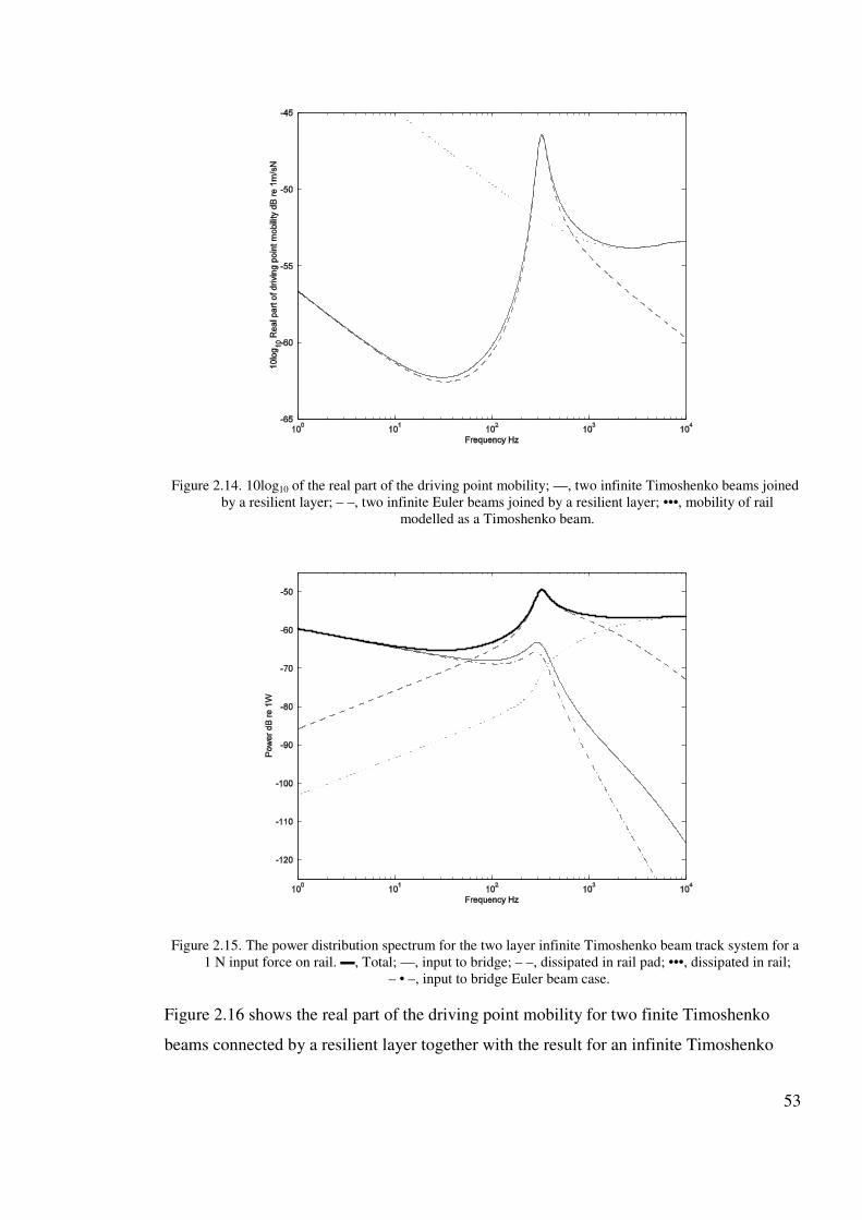
53
Figure 2.14. 10log10 of the real part of the driving point mobility; —, two infinite Timoshenko beams joined by a resilient layer; – –, two infinite Euler beams joined by a resilient layer; •••, mobility of rail
modelled as a Timoshenko beam.
Figure 2.15. The power distribution spectrum for the two layer infinite Timoshenko beam track system for a 1 N input force on rail. ▬, Total; —, input to bridge; – –, dissipated in rail pad; •••, dissipated in rail;
– • –, input to bridge Euler beam case.
Figure 2.16 shows the real part of the driving point mobility for two finite Timoshenko
beams connected by a resilient layer together with the result for an infinite Timoshenko
54
beam system (Figure 2.14) and the finite Euler beam system (Figure 2.12) for comparison.
Comparing first the finite and infinite Timoshenko systems, it can be seen that although
peaks due to reflections at the ends of the beams can be seen in the finite result, the general
trends of both systems are the same.
As for the finite the Euler beam system in Figure 2.12 at low frequencies, modelling the
effect of finite beams results in deviations of more than 10 dB about the infinite result.
Above 10 Hz the Euler formulation begins to over-predict the frequency at which each
mode occurs. It will be shown later that this may not be significant in terms of a complete
bridge noise calculation. However it highlights another source of error arising from using
an Euler formulation rather than a Timoshenko formulation.
Figure 2.16. 10 log10 of the real part of the driving point mobility against frequency. —, Two finite 100 m Timoshenko beams joined by a resilient layer excited at 22 m along span; – –, infinite case;
– • –, finite Euler case.
2.7. SUMMARY
An improved method for the calculation of the power input to a bridge has been described.
The method is based on (Thompson, 1992) but has been developed to include extra layers
of mass and resilience. This enables the model to be applied to a broad range of track
forms. The approach also has been developed to include the effects of a finite bridge length
and the use of Timoshenko beam theory to model the rail and bridge. The results suggest

55
that these new features, particularly the inclusion of the finite effects of the bridge at low
frequencies, should be included to provide an accurate calculation of the power input to the
bridge. The outcome is an improved model for the power input to the bridge that greatly
enhances the ability to determine the effects of resilient track fastenings on bridge noise.

56
3. THE MOBILITY OF A BEAM
In the previous chapter a model for a rail coupled to a bridge beam was presented. This
model is particularly useful for frequencies below the decoupling frequency. At frequencies
higher than the decoupling frequency, the two beams vibrate independently. Hence the
mobility of each beam becomes more important. Moreover, for reasons presented in this
chapter, the bridge can no longer be modelled as a beam at very high frequencies due to
local effects within the beam profile. This leads to the search for an appropriate calculation
model for the mobility of a bridge for frequencies greater than about 200 Hz. This chapter is
concerned with the development of such a calculation of the input mobility of an I-section
beam which forms the basis of many bridges (Janssens and Thompson, 1996).
Cremer, Heckl and Ungar (1986) present equations for the point mobility for a number of
infinite structures. Of relevance to this work is an equation for the point mobility of an
infinite beam of finite depth discussed in Section 3.5 below. Petersson (1983) developed a
semi-empirical model for the point mobility at the intersection of two perpendicular plates,
by modelling the T-section as an elastic half space and calibrating the result to fit measured
data. Pinnington (1988) presented an approximate model for the same structure. He
concluded that at low frequencies, the point mobility of the T-section is the same as that of a
semi-infinite edge-excited flat plate. At higher frequencies the mobility of the T-section
tends to that of the top plate.
Petersson (1999) went on to develop a numerical model of an infinite rectangular cross-
section beam of finite depth. Accompanying this numerical model he developed equations to
estimate the point mobility in four frequency ranges. At low frequencies, below the first
quasi-longitudinal (transitional) mode, the point mobility is modelled as in (Cremer, Heckl
and Ungar, 1986). Beyond this mode and for Helmholtz numbers (kTl, where kT is the
transverse wave number and l is the radius of contact patch) less than unity, the point
mobility is modelled as in (Pinnington 1988). For Helmholtz numbers above unity, the point
mobility is said to tend towards that of a rod with cross-sectional dimensions of the beam
height and thickness. The current work takes this further by developing an estimate of the
driving point mobility of an I-section beam within three frequency ranges and
demonstrating, using calculations for the driving point mobility of an infinite beam, that the

57
results can be used as a spatial average of the driving point mobility of a finite beam.
3.1. FINITE ELEMENT MODEL OF RECTANGULAR SECTION BEAMS
Before considering approximate formulae for the mobility of a beam, mobility spectra for
typical length beams against which such formulae can be evaluated have been produced
using a finite element model. For this purpose the ANSYS finite element software has been
used. Clearly to obtain valid results at high frequencies a detailed mesh is required. To avoid
the model becoming too large only simple geometry is considered.
In the first step of the finite element study a simply supported rectangular cross-section
beam, 20 m in length, is considered. This is typical of a major structural component of a
railway bridge. The model omits, at this stage, the flange from the I-shaped girder firstly for
simplicity and secondly as a good first step from which to evolve a model of a complete I-
section beam. Figure 3.1 shows the shape of the cross-section used and its dimensions. The
material properties of steel are used.
1.0m 0.02m y
x z
Figure 3.1. A schematic of the cross section used in the finite element study.
The elements used are two-dimensional elements having membrane (in-plane4) stiffness but
no bending (out-of-plane) stiffness. The element has two degrees of freedom at each of its
eight nodes: translations in the nodal x and y directions.
To ensure accuracy of the finite element model, the element length in the x-direction should
not exceed 41 of the shear wavelength in steel (i.e. eight nodes per wavelength). This can
be calculated from the shear wave speed given by,
steel
steels
Gc
ρ= (3.1)
4 As only vertical motion of the beam is considered as part of the bridge modelling approach described in
(Thompson & Jones, 2002) only in-plane motion is considered here.

58
where Gsteel and ρsteel are the shear modulus and density of steel. This gives a shear wave
speed of 3130 m/s. Therefore for the mesh to contain approximately eight nodes per shear
wavelength at 10 kHz, an element length of 0.08 m was used. In a similar way, the element
length needed in the y-direction was calculated from the longitudinal wave speed, given by,
( )21 νρ −=
steel
steell
Ec (3.2)
where Esteel is the Young’s modulus and ν is Poisson’s ratio, giving cl = 5200 m/s. The
element length required in the y-direction was calculated as 0.13 m. Approximately 1900
elements have therefore been used in the mesh. For efficiency, the number of elements can
be reduced by the use of symmetry. Only a quarter of the beam is modelled with four
different boundary conditions. The four separate solutions are then added together to gain a
result for the whole beam. Figure 3.2 shows a diagram of how this is achieved and Table 3.1
shows the boundary conditions used for each solution. The anti-symmetric condition at a
corresponds to the simple supports considered in the previous chapter. The splitting of the
model into four sections means that the number of elements in each mesh is reduced to
approximately 480.
A direct solution method was used and damping was included in the model using a constant
damping ratio of 0.05.
Figure 3.2. The geometrical model of the beam split into 4 symmetrical sections. The quarter shown shaded is the quarter modelled with different boundary conditions on edges a, b and c.
Boundary conditions at edge a
Boundary conditions at edge b
Boundary conditions at edge c
Solution 1 anti-symmetric anti-symmetric anti-symmetric
Solution 2 anti-symmetric symmetric anti-symmetric
Solution 3 anti-symmetric symmetric symmetric
Solution 4 anti-symmetric anti-symmetric symmetric Table 3.1. Boundary conditions needed to model beam by symmetry.
3.1.1. FE results
A solution was obtained for the frequency range 1 to 10 kHz, with a frequency resolution of
a
b
c

59
1 Hz for 1 to 500 Hz, 2 Hz for 500 to 1000 Hz and 10 Hz for 1000 to 10000 Hz. The beam
was loaded with a sinusoidal 1 N nodal force at 7.2 m from the beam end and the complex
amplitude of deflection at this point was extracted from the results. The amplitude of the
deflection was then used to calculate the driving point mobility for the beam, shown in
Figure 3.3.
The first mode occurs at approximately 6 Hz. The modal contribution of the various beam-
type modes can be distinctly seen up to about 1 kHz. Beyond 1 kHz the modal density
becomes too high to distinguish the contribution from individual modes.
The sudden rise in point mobility at 2.5 kHz is due to the occurrence of the first longitudinal
mode within the depth of the cross-section and could be described as the transitional mode
between high and mid-frequency behaviour. Due to the very high modal density around this
frequency, a single mode shape that demonstrates this clearly could not be found, but
longitudinal waves in the vertical plane of the beam are expected to begin occurring at
approximately 2.5 kHz, which is the frequency at which the longitudinal wavelength is
approximately twice the depth of the beam.
Figure 3.3. The real part of driving point mobility plotted against frequency for a 20 × 1 × 0.02 m rectangular
cross-section beam.

60
3.1.2. Effect of position on driving point mobility
The contribution from each mode of the beam to the mobility is not uniform as the
excitation point is moved along the length of the beam; it varies with the position of the
excitation force with respect to the nodes of each mode of the beam. For this reason, an
average has been taken of the real part of the driving point mobility for excitation at a
number of points along the beam. Figure 3.4 shows the real part of the mobility at 7 m,
4.2 m, 2.4 m and 1.1 m from one end of the beam. At low frequency the variation in the real
part of the mobility is large. The variation diminishes as frequency and the modal density
increases. Above about 1 kHz the variation is small.
Figure 3.4. The real part of driving point mobility plotted against frequency taken at four points on a
20 × 1 × 0.02 m beam. , 7 m; •••, 4.2 m; − −, 2.4 m; − • −, 1.1 m; ▬, average.
3.1.3. Effect of varying length and depth
FE studies were performed on beams with dimensions 10 × 1 × 0.02 m, 10 × 0.5 × 0.02 m,
5 × 1 × 0.02 m, 5 × 0.5 × 0.02 m, 3 × 1 × 0.02 m and 3 × 0.5 × 0.02 m. The average driving
point mobility of four points on the beam is again determined. This is plotted in Figure 3.5
and Figure 3.6.
When the length of the beam is halved, but the depth is kept the same (Figure 3.5) the
fundamental frequency increases by a factor of four. This follows the expression for the nth

61
flexural natural frequency ωn of an Euler beam which is given by,
A
EI
ln
ρ
πω
2
= (3.3)
Equation (3.3) shows that the frequency of the fundamental mode is directly proportional to
the depth of the beam as I ∝ d3 and A ∝ d as can be seen in the FE results.
The transitional modes of the 1 m deep beams occur at precisely the same point as for the
20 × 1 × 0.02 m beam, which confirms that this mode is not a function of length, but of
depth. The results from the 0.5 m deep beams (Figure 3.6) show that a decrease in depth by
a factor of two increases the frequency of the transitional mode by a factor of two to about
5 kHz. This is consistent with the assumption that the transition is associated with the cut-on
of in-plane compression. The natural frequency of quasi-longitudinal waves is given by,
)1( 2νρ
πω
−=
E
d
nn (3.4)
where d is the depth of the beam, so ωn is directly proportional to the inverse of depth.
Figure 3.5. The spatially averaged real part of driving point mobility against frequency for various 1 m deep
rectangular section beams. , 20 × 1 × 0.02 m; − −, 10 × 1 × 0.02 m; •••, 5 × 1 × 0.02 m; − • −,
3 × 1 × 0.02 m.

62
Figure 3.6. The spatially averaged real part of driving point mobility against frequency for various 0.5 m deep
rectangular section beams. , 10 × 0.5 × 0.02 m; − −, 5 × 0.5 × 0.02 m; •••, 3 × 0.5 × 0.02 m.
3.1.4. Effect of varying thickness.
In order to investigate the effect of varying the beam thickness on the real part of the driving
point mobility, additional finite element solutions were calculated for 3 × 1 × 0.01 m and
3 × 1 × 0.04 m beams. Figure 3.7 shows the real part of the driving point mobility for each
beam plotted against frequency. It can be seen that varying the thickness has negligible
effect on the frequency characteristics of the mobility. As the thickness of the cross-section
increases the overall level of the mobility reduces. This is expected, as increasing the
thickness of the cross-section will increase the beam’s stiffness and mass in the same
proportions.
3.1.5. Effect of varying damping
Figure 3.8 shows the average real part of the driving point mobility taken from four points
along a 3×1×0.02 m beam, while varying the damping ratio (ζ). In the low frequency range,
increasing ζ lowers the magnitude at resonance peaks and raises the troughs between them.
At high frequencies, increasing the damping raises the average level of the mobility. This
effect begins to happen around the second natural frequency of the 3 × 1 × 0.02 m beam and
the variation of the real part of the driving point mobility is at its largest in the transitional
region around 1.5 kHz. As frequency is increased further, increasing ζ still raises the overall

63
level of the mobility, but the variation in levels is smaller.
Figure 3.7. The spatially averaged real part of driving point mobility against frequency for three 3 × 1 m
beams of varied thickness., h = 0.02 m; •••, h = 0.01 m; − −, h = 0.04 m.
Figure 3.8. The spatially averaged real part of driving point mobility against frequency for a 3 × 1 × 0.02 m
beam. , ζ = 0.05; •••, ζ = 0.025; − −, ζ = 0.1.
3.2. BEAMS WITH A FLANGE
The next step of the study is to add a representation of the flange to the geometrical model
of the girder to see how the addition of such a component will affect the driving point

64
mobility. The flange is likely to have a highly frequency dependent effect on the result. At
low frequencies the motion of the web and flange is strongly coupled and the system is
likely to behave like the rectangular section beam, but with different values of A and I. The
mass of the flange is expected to influence the frequency of the transition mode. At
frequencies above the decoupling frequency, the flange will behave independently of the
web.
The aim of the next stage in the FE modelling is to examine these effects and to discover
how wide the flange can be before this effect is seen. Following this next stage in the FE
study, a better understanding of how the flange affects the point mobility of the girder, and
of the transition between thick beam behaviour and thin plate behaviour will be gained.
3.2.1. Beam representation of a flange
In order not to add too many degrees of freedom to the FE model, the flanges are modelled
first as two identical beams, placed on the top and bottom of the web. The elements used to
represent the beams are two-node beam elements, which have an associated cross-sectional
area A, depth d and second moment of area I, which can be changed for each study to
simulate changing the width of the flange. This means that no extra nodes will be added to
the model, as no bending will occur within the flange apart from the bending associated with
the web. Any effects seen by adding the beams to the web should simply be those associated
with adding extra mass and bending stiffness to the top and the bottom of the web, as this
flange will not behave independently from the web.
Figure 3.9 shows a schematic representation of the cross-section to be used in this part of the
study. The FE study was performed on a 3 × 1 m beam as discussed above. As well as
keeping the model small, the depth of 1 m meant that the transitional mode would occur
lower in the frequency range than it would in a 0.5 m depth beam, making it a better model
for the study of the transition between mid and high-frequency behaviour. The model was
used to include a beam representing a 10 cm, 20 cm and 40 cm flange (full width) 0.02 m
thick in each case.
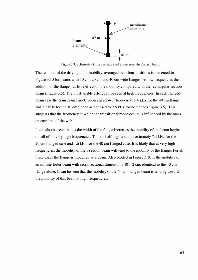
65
.02 m
t f
.0 2 m
membrane elements
beam elements
Figure 3.9. Schematic of cross section used to represent the flanged beam.
The real part of the driving point mobility, averaged over four positions is presented in
Figure 3.10 for beams with 10 cm, 20 cm and 40 cm wide flanges. At low frequencies the
addition of the flange has little effect on the mobility compared with the rectangular section
beam (Figure 3.5). The most visible effect can be seen at high frequencies. In each flanged-
beam case the transitional mode occurs at a lower frequency, 1.4 kHz for the 40 cm flange
and 2.2 kHz for the 10 cm flange as opposed to 2.5 kHz for no flange (Figure 3.5). This
suggests that the frequency at which the transitional mode occurs is influenced by the mass
on each end of the web.
It can also be seen that as the width of the flange increases the mobility of the beam begins
to roll off at very high frequencies. This roll off begins at approximately 7.4 kHz for the
20 cm flanged case and 4.6 kHz for the 40 cm flanged case. It is likely that at very high
frequencies, the mobility of the I-section beam will tend to the mobility of the flange. For all
these cases the flange is modelled as a beam. Also plotted in Figure 3.10 is the mobility of
an infinite Euler beam with cross-sectional dimensions 40 × 2 cm, identical to the 40 cm
flange alone. It can be seen that the mobility of the 40 cm flanged beam is tending towards
the mobility of this beam at high frequencies.

66
Figure 3.10. Real part of driving point mobility, averaged at four positions, of an I-section beam with the
flange modelled as a beam. , 10 cm flange; − −, 20 cm flange. •••, 40 cm flange; −−−− • −−−−, infinite Euler
beam with cross sectional dimensions 40 × 2 cm.
3.2.2. Shell representation of flange
Representing the flange with beam elements allowed the effect of adding a mass to the top
and bottom of the girder to be seen. The model is closer to that of an I-section beam than in
the earlier studies, but it is still an unrealistic I-section. The addition of a flange that would
allow bending within its width will have a more realistic effect on the driving point mobility
of the girder, such as the addition of an ‘effective’ mass to the top and bottom of the web
rather than an actual mass.
The cross section used for this study was the same as in Figure 3.9, but eight-noded plate
elements were used to model the flange rather than beam elements. To allow eight nodes per
bending wavelength in the width of the flange at 10 kHz an element edge length of 0.034 m
was calculated, according to,
( ) ωνρ
42
2
112 −=
EhcB (3.5)
where cB is the bending wave speed. As before, a 3 × 1 m beam was modelled. The addition
of a flange that would allow bending within its width greatly increases the size of the model
used. The method using symmetry is therefore employed in this study. The beam was split
into four sections (Figure 3.11) along the two axes of symmetry, so that only one quarter

67
of the flange is used in each solution. This model was used to study beams with flanges of
total width 10 cm, 20 cm and 40 cm.
1 2
3 4
Figure 3.11. The girder split into 4 sections by symmetry.
The real part of the driving point mobility averaged over four positions along the beam is
presented for each beam in Figure 3.12 to Figure 3.14. For the 10 cm flanged beam, the
flange does not decouple from the web until approximately 5 kHz and acts as a lumped mass
along the top and bottom of the web below this frequency. The addition of this mass lowers
the frequency of the transitional mode from 2.5 kHz (Figure 3.3) to about 2.1 kHz
(Figure 3.12) as already seen for the beam model of the flange. For the 20 cm flange the
transitional mode occurs at an even lower frequency (Figure 3.13). However the transitional
mode appears to rise again for the 40 cm flange (Figure 3.14), suggesting more complex
behaviour controlling the longitudinal modes in the beam than a simple added mass effect.
For the 20 cm flange, the flange is subject to bending modes and a decoupling of the flange
mass occurs at approximately 1.2 kHz where a half wavelength fits in the width of the
flange. Pinnington (1988) suggests that above this frequency the apparent mass and
therefore its effect on the web is reduced. However at very high frequency where the
wavelengths in the web are very small so that the web is decoupled, the mobility tends to
that of the bending waves in the flange. The mobility of the flange modelled as an infinite,
normally excited plate is plotted in Figure 3.12 to Figure 3.14. The combined mobilities of
the infinite plate flange and the infinite, edge-excited web plate (described later) are also
plotted in Figure 3.12 to Figure 3.14. It can be seen that the mobility of the finite element
model tends towards this latter curve at the upper limit of frequency for which results are
given.

68
Figure 3.12. Real part of driving point mobility of 10 cm flanged I-section beam: ▬, average FE result; •••,
coupled flange and web mobility; − −, edge-excited plate mobility; − • −, mobility of flange.
Figure 3.13. Real part of driving point mobility of 20 cm flanged I-section beam: ▬, average FE result; •••,
coupled flange and web mobility; − −, edge-excited plate mobility; − • −, mobility of flange.

69
Figure 3.14. Real part of driving point mobility of 40 cm flanged I-section beam: ▬, average FE result; •••,
coupled flange and web mobility; − −, edge-excited plate mobility; − • −, mobility of flange.
3.3. A SIMPLE MODEL FOR THE DRIVING POINT MOBILITY AT LOW FREQUENCIES
The finite element studies have shown the effects that are important to consider in modelling
I-section beams. For the calculation of the driving point mobility of a bridge from the
geometry of the bridge beneath the track fastener a simple rapid calculation is sought that is
suitable for the modelling approach adopted.
3.3.1. Infinite beam models
The range 1 Hz to 500 Hz is important for the excitation of structure-borne noise by the
vehicle and track. Soft base-plates are usually designed to isolate vibration at low
frequencies. In order to study the behaviour of vibration isolating track design an accurate
approximation of the point mobility of the girder at low frequencies is needed. Assuming
that a typical bridge deck can be represented as an I-shaped girder, at low frequencies the
bridge mobility can be considered to be that of a Timoshenko beam as,
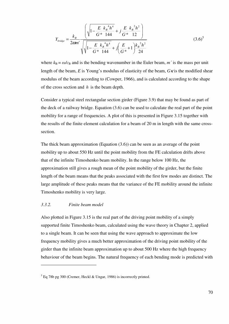
70
241
*144*1
12*144*1
'2 2244
2244
hk
G
Ej
hk
G
E
hk
G
Ej
hk
G
E
m
kY
BB
BB
Bbridge
++−
+−
=ω
(3.6)5
where kB = ω/cB and is the bending wavenumber in the Euler beam, m΄ is the mass per unit
length of the beam, E is Young’s modulus of elasticity of the beam, Gκ is the modified shear
modulus of the beam according to (Cowper, 1966), and is calculated according to the shape
of the cross section and h is the beam depth.
Consider a typical steel rectangular section girder (Figure 3.9) that may be found as part of
the deck of a railway bridge. Equation (3.6) can be used to calculate the real part of the point
mobility for a range of frequencies. A plot of this is presented in Figure 3.15 together with
the results of the finite element calculation for a beam of 20 m in length with the same cross-
section.
The thick beam approximation (Equation (3.6)) can be seen as an average of the point
mobility up to about 550 Hz until the point mobility from the FE calculation drifts above
that of the infinite Timoshenko beam mobility. In the range below 100 Hz, the
approximation still gives a rough mean of the point mobility of the girder, but the finite
length of the beam means that the peaks associated with the first few modes are distinct. The
large amplitude of these peaks means that the variance of the FE mobility around the infinite
Timoshenko mobility is very large.
3.3.2. Finite beam model
Also plotted in Figure 3.15 is the real part of the driving point mobility of a simply
supported finite Timoshenko beam, calculated using the wave theory in Chapter 2, applied
to a single beam. It can be seen that using the wave approach to approximate the low
frequency mobility gives a much better approximation of the driving point mobility of the
girder than the infinite beam approximation up to about 500 Hz where the high frequency
behaviour of the beam begins. The natural frequency of each bending mode is predicted with
5 Eq 78b pg 300 (Cremer, Heckl & Ungar, 1986) is incorrectly printed.
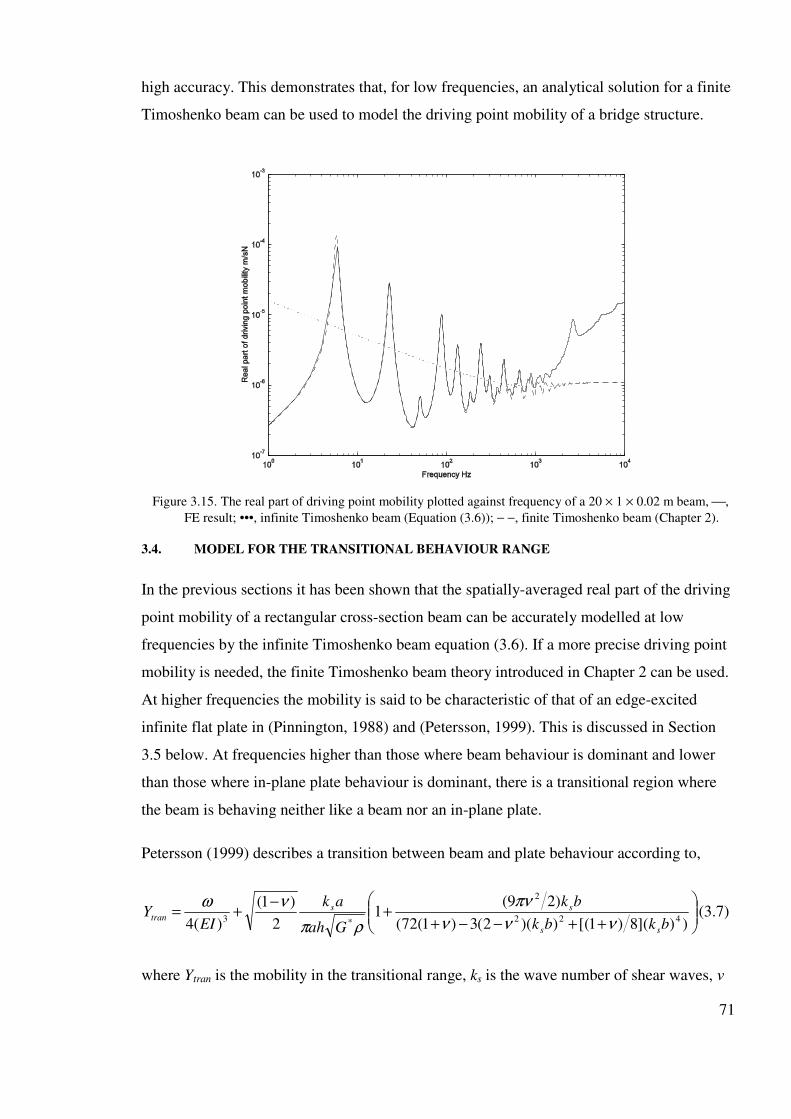
71
high accuracy. This demonstrates that, for low frequencies, an analytical solution for a finite
Timoshenko beam can be used to model the driving point mobility of a bridge structure.
Figure 3.15. The real part of driving point mobility plotted against frequency of a 20 × 1 × 0.02 m beam, ,
FE result; •••, infinite Timoshenko beam (Equation (3.6)); − −, finite Timoshenko beam (Chapter 2).
3.4. MODEL FOR THE TRANSITIONAL BEHAVIOUR RANGE
In the previous sections it has been shown that the spatially-averaged real part of the driving
point mobility of a rectangular cross-section beam can be accurately modelled at low
frequencies by the infinite Timoshenko beam equation (3.6). If a more precise driving point
mobility is needed, the finite Timoshenko beam theory introduced in Chapter 2 can be used.
At higher frequencies the mobility is said to be characteristic of that of an edge-excited
infinite flat plate in (Pinnington, 1988) and (Petersson, 1999). This is discussed in Section
3.5 below. At frequencies higher than those where beam behaviour is dominant and lower
than those where in-plane plate behaviour is dominant, there is a transitional region where
the beam is behaving neither like a beam nor an in-plane plate.
Petersson (1999) describes a transition between beam and plate behaviour according to,
++−−++
−+=
))](8)1([))(2(3)1(72(
)29(1
2
)1(
)(4 422
2
*3bkbk
bk
Gah
ak
EIY
ss
sstran
ννν
πν
ρπ
νω(3.7)
where Ytran is the mobility in the transitional range, ks is the wave number of shear waves, ν
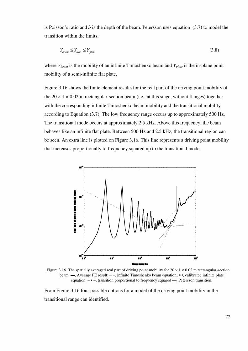
72
is Poisson’s ratio and b is the depth of the beam. Petersson uses equation (3.7) to model the
transition within the limits,
platetranbeam YYY ≤≤ (3.8)
where Ybeam is the mobility of an infinite Timoshenko beam and Yplate is the in-plane point
mobility of a semi-infinite flat plate.
Figure 3.16 shows the finite element results for the real part of the driving point mobility of
the 20 × 1 × 0.02 m rectangular-section beam (i.e., at this stage, without flanges) together
with the corresponding infinite Timoshenko beam mobility and the transitional mobility
according to Equation (3.7). The low frequency range occurs up to approximately 500 Hz.
The transitional mode occurs at approximately 2.5 kHz. Above this frequency, the beam
behaves like an infinite flat plate. Between 500 Hz and 2.5 kHz, the transitional region can
be seen. An extra line is plotted on Figure 3.16. This line represents a driving point mobility
that increases proportionally to frequency squared up to the transitional mode.
Figure 3.16. The spatially averaged real part of driving point mobility for 20 × 1 × 0.02 m rectangular-section
beam. ▬, Average FE result; − −, infinite Timoshenko beam equation; •••, calibrated infinite plate
equation; − • −, transition proportional to frequency squared , Petersson transition.
From Figure 3.16 four possible options for a model of the driving point mobility in the
transitional range can identified.

73
1. The trivial option is to model the driving point mobility in the transitional region
as a vertical jump up to the infinite flat plate behaviour at the frequency at which the
transitional mode occurs. In the case of a 20 × 1 × 0.02 m beam, it can be seen that
modelling the transitional range with the trivial solution means that the model always
underestimates the driving point mobility in this range.
2. Another option is to model the driving point mobility as flat plate behaviour from
the point at which the driving point mobility of the infinite flat plate is higher than the
infinite Timoshenko mobility as adopted by (Janssens & Thompson, 1996). This would
result in an over-estimation of the driving point mobility in this range. Moreover, modelling
the transition with the infinite flat plate equation is physically unrealistic, as the beam cannot
behave as an infinite flat plate until the first quasi-longitudinal mode has occurred.
3. The third option is to model the transition according to equation (3.7). From
Figure 3.16 it can be seen that between 1 kHz and 1.7 kHz the agreement between the FE
results and equation (3.7) is good. However the sudden rise up to the mobility of the infinite
plate results in an over-estimate of the point mobility thereafter.
4. The fourth option is to model the driving point mobility as rising in proportion to
frequency squared until the transitional mode is reached. This is an empirical method,
chosen because it fits the general trend of the FE-calculated driving point mobility in this
region. Above 1 kHz the frequency-squared model agrees very well with the finite element
results.
Figure 3.17 shows the finite element results of the driving point mobility of a 3 × 1 × 0.02 m
rectangular-section beam together with its corresponding infinite Timoshenko and infinite
in-plane plate equations, and with corresponding frequency-squared and Petersson models
for the transitional range. The infinite flat plate model gives an over-estimation of the
driving point mobility in the transitional range for this case. For this case the Petersson
model gives a reasonable estimation of the point mobility between 1 kHz and 1.7 kHz, but
again the rise up to plate behaviour at this point results in an over-estimation of the point
mobility. Agreement between the frequency-squared model and the finite element results
above 1 kHz is good. Although it is only based on empirical considerations, the frequency-
squared transition is adopted here as the practical approach.

74
Figure 3.17. The spatially averaged real part of driving point mobility of a 3 × 1 × 0.02 m rectangular-section
beam. ▬, Average FE result; − −, infinite Timoshenko beam equation; •••, calibrated infinite plate
equation; − • −, transition proportional to frequency squared , Petersson transition.
3.5. MODEL FOR THE MOBILITY AT HIGH FREQUENCY
It has been seen that a transitional frequency occurs that is associated with the cut-on of in-
plane waves in the beam. Still considering a beam without flanges, the behaviour in the
frequency region above the transition may therefore be assumed to be characteristic of that
of an edge-excited flat plate. Two approximate formulae for the behaviour in this region
have been found in the literature:
1. Pinnington (1988) considers the mobility at the junction of two plates forming a
‘T’ shape. For the mobility in the vertical direction, at high frequency the flange plates may
be considered to have relatively short bending wavelengths and therefore to decouple
effectively from the vertical plate of the ‘T’. Pinnington proposes the following formula for
the mobility of an edge-excited plate based on half the force applied at the centre of an
infinite plate and which therefore ignores the effect of the plate edge. The second term
consists of a term due to compressional waves and a term due to a shear waves.
( )
+
−+
−=
GhEhEa
iYbridge
11
42
1 22 νωνω (3.9)
where a is the excitation radius and G is the shear modulus. The excitation radius is the

75
radius of the area over which the excitation force is acting. According to (Pinnington, 1988),
a must be less than h/2. When G and E are considered as real quantities and hysteretic
damping is not included, the first term represents the imaginary part of the driving point
mobility with the second term representing the real part of the driving point mobility. When
considering the power input to the bridge, only the real part is of interest and the excitation
radius does not affect the result.
2. Petersson (1999) proposes, in his study of a rectangular section beam, to use the
formula,
ρπ Gh
kY S
bridge = (3.10)
in which ks is the shear wave number and h is the thickness of the beam. This is also based
on an approximate consideration of an edge-excited infinite plate and which also ignores the
effects of the edge of the plate.
Figure 3.18 shows the two alternative estimates of the high frequency infinite-beam
mobility, equations (3.9) and (3.10), compared with the Finite Element result for a 20 m
beam in the frequency range 1 kHz to 10 kHz. It can be seen that both infinite-beam
estimates fall a little below the finite element calculated mobility. Possible sources for the
discrepancy between the infinite plate approximations and the finite element model must be
investigated in order to study the formulae further:
1. The finite element model is loaded at a single node rather than over an excitation
radius. Moreover, it is not clear how the nodal force and the shape functions of the element
approximate the near-field behaviour of the edge of the beam. This approximation in the FE
method will become significant as the wavelengths in the plate become small at high
frequency.
2. The approximations in both the equations (3.9) and (3.10) ignore the effects of the
edge on the vibration propagation at the excitation patch.
3. Neither of the two infinite plate approximations includes the effects of damping. A
high level of damping has been included in the finite element model in order to produce a
smooth curve. Figure 3.8 shows that the variation of the mean level of mobility with

76
damping is small, however this conclusion must be checked after point 1 has been
investigated.
Figure 3.18. The spatially averaged real part of driving point mobility of 20 × 1 × 0.02 m beam, , FE result;
− −, Pinnington equation (3.9); •••, Petersson equation (3.10).
3.5.1. Boundary element model
In order to study the issues 1 to 3 above, this phase of the investigation aims to calibrate the
infinite plate equation and refine the finite element mesh used. The structural boundary
element software GBED4, which has been developed for ground vibration problems (Jones
& Thompson, 1999), is used for this purpose. The GBED4 software can be used to study the
surface of the beam efficiently without the need for a large number of elements. In the
boundary element method a load is applied as a pressure over an element rather than as the
nodal forces of the finite element method. The simulation of the contact radius in equation
(3.9) by the boundary element numerical model therefore has a more precise meaning than
for the finite element model.
At high frequencies, wavelengths in the beam are short compared with the length and depth
of the beam. The boundary element model provides an infinite length, infinite depth model
of a two-dimensional elastic half-space. Three-noded, quadratic shape function elements
have been used.

77
The GBED4 software allows plane strain problems to be modelled. The case of a bridge
girder is a plane stress problem. Finite element techniques for plane strain problems use a
different stress-strain matrix from that used for plane stress problems, but one is equivalent
to the other if the values of Young’s modulus and Poisson’s ratio entered into the calculation
are changed (Petyt, 1990). Values of E and ν for steel, modified according to (Petyt, 1990),
were used as the material properties for the elastic half space.
To study the effects of the forcing in the near-field, a three-section mesh of the half space
surface was created (Figure 3.19). A ‘near-field’ mesh is defined, which extends each side of
the contact radius to one quarter of the longitudinal wavelength at the lowest frequency
studied and another section is added on each side of the near-field mesh to create right and
left hand ‘far-field’ meshes. These sections extend out to twice the longitudinal wavelength
at the lowest frequency studied to ensure that the model approximates an infinite half space.
The element length in the near field mesh is set to 1/15 of the shear wavelength6 of the
highest frequency studied to allow for accurate investigation of the near-field effect. The
element length in the far field is set to 2/5 of the shear wavelength of the highest frequency
studied.
At the origin of the half space, one small element is placed in the mesh. The forcing of the
half space is distributed over the length of this element and its length is equal to twice the
required contact radius. In this case the contact radius is set to 0.01 m, which is equal to half
the thickness of most of the beams studied so far.
6 This figure was chosen after investigation showed that results had converged when 15 elements per shear
wavelength were used.

78
.
2λ pmin
λ pmin /4
Left hand far field mesh Right hand far field mesh Near field mesh
Loaded element
Figure 3.19. Diagram of mesh used in GBED4
3.5.2. Boundary element results
A solution was obtained for the steel elastic half space for five frequencies between 1 kHz
and 10 kHz. Figure 3.20 shows the displacement along the surface of the half space at
1 kHz. The peak at the load can be seen at the origin. Each side of the origin, extending
approximately 1 m, a near-field wave can be seen that has an exponential shape rather than
the sinusoidal shape that is seen further out to the edges of the half space. The element size
used in the horizontal direction in the finite element model of the previous studies was not
sufficiently small to model this effect accurately.
Figure 3.20. Normal displacement on the surface of the steel half space at 1 kHz.
The boundary element analysis highlights a requirement for a more carefully defined finite
element model for this frequency range. Adding a near-field mesh to the previous finite
element models, containing smaller elements, ensures that the near-field effects are
accurately modelled. To model the loading radius more precisely, the forcing on the finite
element mesh was altered so that the load acts across an element of the appropriate size

79
rather than just at one node. Figure 3.21 shows how a force F is placed across an element to
approximate pressure loading over an element (Petyt, 1990).
A solution was obtained from a refined 3 × 1 × 0.02 m finite element model for the range
1 kHz to 10 kHz. Figure 3.22 shows the real part of the driving point mobility obtained from
the boundary element results plotted with results from the previous and refined finite
element models. The refinement of the mesh and the loading in the finite element model has
had negligible effect around the transitional mode at approximately 2.5 kHz. However in the
ranges 1 kHz to 2 kHz and 3 kHz to 10 kHz the overall level of the driving point mobility
for the refined finite element mesh is slightly higher than that of the unrefined mesh. Good
agreement can be seen between the boundary element result and the refined finite element
result. This suggests that the boundary element elastic half space provides a good
approximation for the average behaviour of the beam in this frequency range. The average
point mobility in this region is therefore dependent only on the material properties and
damping of the beam, not the geometry. However the boundary element model is unsuitable
for the purposes of the bridge model. A correction to equation (3.9) that would accurately
replicate the results of the boundary element model is therefore sought.
F6
1 F
6
1
F3
2
Figure 3.21. Diagram of how a load is distributed to model a pressure applied along the side of an element in
the finite element model.

80
Figure 3.22. The spatially averaged real part of driving point mobility of refined mesh FE model and BE
model. ▬, refined FE; , unrefined FE; − −, BE result;
3.5.3. Calibration of in-plane plate equation
The in-plane plate equation (3.9) does not contain damping. To calibrate the infinite plate
equation to fit the boundary element result, a boundary element solution was performed with
a very low value of damping in the model7. This result is shown in Figure 3.23 and an
approximate factor of 1.13 has been found between it and equation (3.9).
The real part of equation (3.9) is made up of two terms. The first term (ω(1−ν2)/4Eh)
accounts for the effect of longitudinal waves in the plate and the second term (ω/4Gh)
accounts for the effect of shear waves. The second term may be written as a function of
shear wave number (ω/4ρcs2h). In order to take better account of the effect of the edge of the
plate the shear wave speed can be replaced by the Rayleigh wave speed, (ω/4ρcR2h). It is
found that this accounts for the 13% difference between (3.9) and the boundary element
result for very low damping.
7 The boundary element model cannot be run with zero damping since this leads to mathematical instability. A
value of loss factor of 10-5 was therefore used.
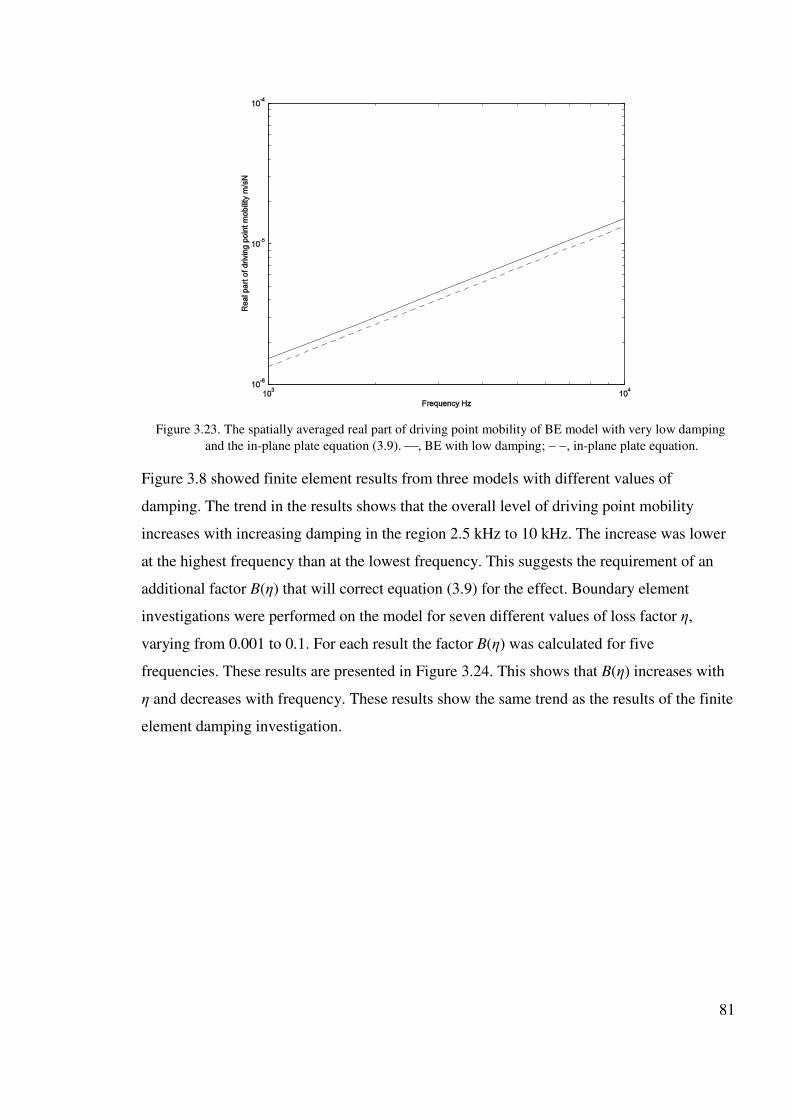
81
Figure 3.23. The spatially averaged real part of driving point mobility of BE model with very low damping
and the in-plane plate equation (3.9). , BE with low damping; − −, in-plane plate equation.
Figure 3.8 showed finite element results from three models with different values of
damping. The trend in the results shows that the overall level of driving point mobility
increases with increasing damping in the region 2.5 kHz to 10 kHz. The increase was lower
at the highest frequency than at the lowest frequency. This suggests the requirement of an
additional factor B(η) that will correct equation (3.9) for the effect. Boundary element
investigations were performed on the model for seven different values of loss factor η,
varying from 0.001 to 0.1. For each result the factor B(η) was calculated for five
frequencies. These results are presented in Figure 3.24. This shows that B(η) increases with
η and decreases with frequency. These results show the same trend as the results of the finite
element damping investigation.

82
Figure 3.24. The factor B(η) for various different values of η at 5 different frequencies. ▬, mean; , 1 kHz;
− −, 1778 Hz; •••, 3162 Hz; − • −, 5623 Hz; −+−, 10 kHz.
Figure 3.25 shows the real part of the driving point mobility from the refined finite element
model and the boundary element results. In each case the loss factor used in the model is
0.1. Figure 3.25 also shows the infinite flat plate equation after modification with a factor
B(η) that is equivalent to the mean B(η) at all five frequencies. The agreement between all
three lines is generally good across the whole frequency range. At 1 kHz the infinite flat
plate equation is approximately 0.6 dB lower than the boundary element result. At 10 kHz
the infinite flat plate result is approximately 0.4 dB higher than the boundary element result.
The errors are due to neglecting the frequency dependence of B(η) when taking the mean.
It is not known what the characteristic damping of bridge beams is at this high frequency
range. The material damping of steel is very low (η ≈ 0.0001) and other effects, such as
friction between the beam and other bridge components may be expected to have little effect
on the point mobility of the beam. In practice therefore, B(η) may be little used and seldom
with a value as high as η = 0.1.
Assuming that B(η) is an accurate representation of the variation of driving point mobility
with loss factor, equation (3.9) becomes,
+
−=
hcEhBY
R
bridge 2
2 11
4)()Re(
ρ
νωη (3.11)

83
Figure 3.25. The spatially averaged real part of driving point mobility against frequency. ▬, refined FE
model; − −, BE model η = 0.1; •••, corrected infinite flat plate equation.
3.6. MODEL FOR THE DRIVING POINT MOBILITY OF AN I-SECTION BEAM
In Sections 3.2 to 3.5, three equations for the real part of the mobility of an infinite
rectangular section beam were derived. It was seen that they gave a good approximation of
the frequency-averaged mobility of a finite beam. Comparison with the finite element study
of an I-section beam in Section 3.2 showed that the equations for frequency-averaged
mobility of the rectangular section beam could be used for the I-section beam in the low and
mid frequency ranges if the parameters A and I were adjusted accordingly. At frequencies
above the transitional mode, it was seen that the mobility tended towards that of a normally
excited flat plate due to the addition of the flange. It was also seen that the addition of the
flange moved the transitional frequency. Hence the marker for the beginning of high
frequency behaviour was moved and found not to be simple to predict. This section is
concerned with the investigation of the mechanisms that determine the transitional
frequency by taking a different modelling approach and aims to predict this frequency with
reasonable accuracy.
3.6.1. Motivation
The frequency at which the first in-plane longitudinal mode of the beam occurs has been

84
termed the ‘transitional’ frequency. In the finite length beams that have been studied so far
the modal deformation in this mode is coupled with longitudinal strain and no single mode
where only vertical stretching is seen can be easily identified. The addition of the flange
(mass) to each end of the rectangular cross section lowers the frequency at which the
transition mode occurs. Above the frequency at which the motion of the flange decouples
from the motion of the web, the flange will act independently of the web and the mass on
each end of the web will become a frequency-dependent apparent mass, approximately the
mass of 1/4 bending wavelength of the flange. This means prediction of the ‘transitional
frequency’ will be more complex for the I-section beam than for the rectangular section
beam. In order to study the dynamics of a flanged beam cross section separately from
longitudinal beam bending effects, a two-dimensional model of the cross section was
produced. The model is developed in stages in Sections 3.6.2 to 3.6.4 below.
3.6.2. Rod with equal masses at each end
M M F′1
u 1 u 2
L
F′1 F′2
F′2 F1 F2
Figure 3.26. The I-section modelled as a rod with equal masses at each end.
The first model (Figure 3.26) comprises a rod representing the web of the cross section of
the beam with a mass at either end representing the flange.
The equation of motion of the rod is given by
02
2
2
=+∂
∂uA
x
uEA ωρ (3.12)
A solution is assumed of the form
ti
LL exkBxkBxu ω))sin()cos(()( 21 += (3.13)
where kL is the longitudinal wave number in the rod and B1 and B2 are constants. These can
be related to the displacement at each end
( ) 11 0 Buu == (3.14a)

85
( ) ( ) ( )LkBLkBLuu LL sincos 212 +== (3.14b)
This can be written in matrix form
( ) ( )
=
2
1
2
1
sincos
01
B
B
LkLku
u
LL
(3.14c)
or
{ } { }BPu 1= (3.14d)
Evaluating the external forces
( ) ( )
2
2
1
00
t
uM
x
uEAF
∂
∂−
∂
∂−= (3.15a)
and
( ) ( )
2
2
2t
LuM
x
LuEAF
∂
∂+
∂
∂= (3.15b)
This can be written in matrix form
( ) ( ) ( ) ( )
++−
−=
2
1
22
2
2
1
sincoscossin B
B
LkMLkEAkLkMLkEAk
EAkM
F
F
LLLLLL
L
ωω
ω (3.15c)
or
{ } { }BPF 2= (3.15d)
Combining (3.14) and (3.15) to eliminate {B}
{ } { }uPPF 1
12
−= (3.16)
where 1
12
−PP is the dynamic stiffness matrix which can be written analytically as
( )( ) ( )
( ) ( )
=
Lk+EAkLkMω-EAk
-EAkLk+EAkLkMω
LkD
LLLL
LLLL
l
wcossin
cossin
sin
12
2
(3.17)
Using (3.17), the point mobility of the cross-section of the I-beam, excited at one end, can

86
be calculated. The point mobility of the system was calculated for various masses (equal) at
each end. These ranged from zero mass (no flange) to 110 kg/m (70 cm flange). Figure 3.27
shows a surface plot of point mobility for each mass against frequency. The red colours
show the peaks in point mobility and the blue colours show the dips. The peaks show the
position of the stretching modes in the cross-section of the beam. It can be seen that as the
flange mass increases, the position of the first mode, or ‘transitional’ mode, decreases in
frequency from approximately 2.5 kHz to 1.3 kHz. This can be expected as the addition of
mass lowers this natural frequency. The same effect can be seen on the higher order
longitudinal modes as well as a reduction of the magnitude of the mobility at the higher
order modes as the flange mass increases.
Figure 3.27. Surface plot of the real part of driving point mobility against frequency for various flange widths.
3.6.3. Rod with equal apparent mass at each end.
Modelling the flange as a fixed mass is an over-simplification as this does not account for
bending in the flange. At low frequency the flange acts as a constant mass on the web. As
frequency increases the bending wavelengths in the flange become comparable to the width
of the flange and the apparent mass of the flange reduces as more of it becomes effectively
decoupled from the web. An estimate of the cut-on frequency of this behaviour is the
frequency at which one quarter of the bending wavelength becomes shorter than the width of
one side of the flange. This frequency can be termed the decoupling frequency. Above this

87
frequency the vibration of the flange and web become uncoupled to some extent and the
mass of the flange acting on the web becomes frequency dependent. An estimate of the
apparent mass is that of one quarter of the bending wavelength of the flange either side of
the web. Thus
fbendfbendapp hhM λλ21
41 )(2 =≈ (3.18)
Mapp and hf are the apparent mass and thickness of the flange and bendλ is the bending
wavelength in the flange.
Plotted in Figure 3.28 is the decoupling frequency plotted against flange width (solid line). It
shows that for flange widths of approximately 15 cm the decoupling frequency occurs at
about 2.3 kHz. This is very close to where the transitional mode occurs. Hence for flange
widths greater than 15 cm only the apparent mass contributes to the transitional mode and it
is no longer affected by flange width, but by the bending wavelength in the flange.
Also plotted in Figure 3.28 is a surface plot of the point mobility of the system, using
apparent mass above the decoupling frequency, for various flange widths. Concentrating on
the transitional mode, for flange widths between 0 and 15 cm, the transition frequency
decreases as the flange width increases. This effect was also seen in the fixed mass model.
However, for flange widths greater than 15 cm the transition frequency no longer decreases
with increasing flange width, but remains constant.

88
Figure 3.28. Surface plot of point mobility against frequency for various flange widths using apparent mass to
model the flange.
3.6.4. Coupled beam and rod model.
The dynamic stiffness method has next been used to model a rod coupled to a beam. This
allows the bending in the flange to be modelled more accurately. Both vertical and lateral
lines of symmetry of the cross-section are used to reduce the problem. The web is modelled
as a rod and the flange is modelled as a beam coupled to the rod (Figure 3.29).
F 1 , u 1
F 2 , u 2
M 2 , θ 2 M 3 , θ 3
F 2 , w 2
F 3 , w 3
b w /2
h w /2
b f /2
Node 2
Node 1
Node 3
Figure 3.29. The I-section modelled as a rod coupled to a sliding-free beam.
The dynamic stiffness matrix of the rod without masses at each end is

89
( )
( )( )
=
2cos1-
1-2cos
2sin wL
wL
wL
Lw
bk
bk
bk
kEAD (3.19)
where Aw = 2wh and is the cross-sectional area of the web if a unit length of the beam is
considered. The equation of motion of the flange beam is
02
4
4
=−∂
∂uA
x
wEI ff ωρ (3.20a)
where Af and If are the longitudinal cross-sectional area and second moment of area of a unit
length of flange.
1×= ff hA (3.20b)
112
3
×=f
f
hI (3.20c)
The bending wavenumber kB in the flange is defined as
41
21
=
f
f
BEI
Ak
ρω (3.21)
so a solution of (3.20a) takes the form
( ) ( ) ( ) ( ) ( )xkBxkBxkBxkBxw BBBB sincossinhcosh 4321 +++= (3.22)
the displacements and rotations are ( )02 ww = , ( )23 fbww = , ( )02 θθ = , ( )23 fbθθ = :
( ) ( ) ( ) ( )( ) ( ) ( ) ( )
−
=
4
3
2
1
3
3
2
2
2cos2sin2cosh2sinh
2sin2cos2sinh2cosh
00
0101
B
B
B
B
bkkbkkbkkbkk
bkbkbkbk
kk
w
w
fBBfBBfBBfBB
fBfBfBfB
BB
θ
θ
(3.23a)
or
{ } [ ]{ }BPw 1= (3.18b)
The nodal forces and moments are ( )02 SF = , ( )23 fbSF −= , ( )02 MM −= ,

90
( )23 fbMM = :
( ) ( ) ( ) ( )( ) ( ) ( ) ( )
−−
−−−
−−
−
=
4
3
2
1
2
3
3
2
2
2sin2cos2sinh2cosh
2cos2sin2cosh2sinh
0101
00
B
B
B
B
bkbkbkbk
bkkbkkbkkbkk
kk
kEI
M
F
M
F
fBfBfBfB
fBBfBBfBBfBB
BB
Bf
(3.24a)
or
{ } [ ]{ }BPF 2= (3.24b)
Combining P1 and P2 to eliminate {B} gives the dynamic stiffness matrix of the flange Df.
The dynamic stiffness matrices of the beam and rod can be coupled at node 2, giving a
dynamic stiffness matrix for the whole system Dcoup. Noting that u2 = w2, yields
=
+
3
3
2
2
1
3
3
2
2
1
44434241
34333231
24232221
141313112221
1211
'
'
0
0
0
000
M
F
M
F
F
w
w
w
w
u
DDDD
DDDD
DDDD
DDDDDD
DD
ffff
ffff
ffff
ffffww
ww
(3.25)
Applying boundary conditions: due to symmetry the beam is sliding at node 2. Therefore
w2′ = 0. The beam is free at its outer edge. Therefore ( ) 023 =−= fbSF and 03 =M .
=
+
0
0
'0
0
00
2
1
3
3
2
1
444241
343331
1413112221
1211
F
F
w
w
w
u
DDD
DDD
DDDDD
DD
fff
fff
fffww
ww
(3.26a)
Modelling the system by symmetry means the system must also be solved with the rod
blocked at the inner end of the web. i.e. 01 =u , giving
=
+
0
0
'
2
3
3
2
444241
343331
14131122 F
w
w
w
DDD
DDD
DDDD
fff
fff
fffw
(3.26b)
For the anti-symmetry case F1 is set to zero in equation (3.26a). By setting 2F to 0.5 in

91
(3.26a) and (3.26b), the response to a unit point force at the top of the I-section can be
found. From this, the point mobility can be calculated.
Figure 3.30 shows a surface plot of the real part of driving point mobility against frequency
for various flange widths. The complex behaviour seen is due to the coupling of bending
modes in the flange and stretching modes in the web. This may help to explain the finite
element results for the flanged beams, where the transitional mode for the 40 cm flange
occurred at a higher frequency than for the 20 cm flange. The mode that occurs at
approximately 1.5 kHz for a flange width of 22 cm and 150 Hz for a flange width of 70 cm
corresponds to the first ‘flange-flapping’ mode of the cross-section and is not a true
stretching mode of the web. However a transitional region can be seen between 1.5 kHz and
3 kHz where the majority of the power in the response occurs. In general the transition
frequency occurs at frequencies slightly lower than when there is no flange present. The
prediction of the exact transition frequency for a given flange width would be complicated
and out of the scope of this project. Nevertheless it can be seen from the study of the three
cross-section models that the apparent mass is an adequate model for predicting this mode,
that is Figure 3.28 gives a good approximation of Figure 3.30.
Figure 3.30. Surface plot of point mobility against frequency for various flange widths using the coupled
model.
3.6.5. Calculation of the transitional mode
Predominantly flange
Transitional
region

92
The model for the frequency-averaged mobility of an I-section beam developed in this
chapter splits the mobility into three frequency ranges. It has been seen in the finite element
results (Sections 3.1-3.2) and the dynamic stiffness method results for the cross section, that
the start of the high frequency behaviour of the beam is marked by the transitional mode.
For the frequency-averaged beam mobility to be calculated in a computer model throughout
the full frequency range it is necessary to calculate the frequency of this transitional mode.
It was shown in section 3.1 that the transitional mode corresponds to the first mode where
longitudinal motion occurs in the web and for a rectangular section beam this mode is
calculated using equation (3.4). In Section 3.6 it was seen that for an I-section beam the
addition of the mass of the flange lowers the frequency at which the transitional mode
occurs. It was also shown that apparent mass is an adequate model for predicting the
transitional mode. Solving for B1 and B2 in equation (3.13) results in the expression
( )wLL bk
k
ktan
1
222
=−µ
µ (3.27)
where wapp AM ρµ = , with Aw the cross sectional area of the rod and bw is the depth of the
web. The first root of this gives the transitional frequency.
3.7. EXPERIMENTS ON WROUGHT IRON I-SECTION BEAM
Figure 3.31 shows a short length of I-section beam. The section had been removed from a
wrought iron railway bridge in Llangamarsh Wells in South Wales and is typical of many
bridges throughout the United Kingdom. The beam is approximately 2.3 m in length and
0.9 m in depth. The length of the beam is insufficient to investigate it’s low frequency
‘bending’ behaviour in the frequency range of interest, however the depth is sufficient for
investigating it’s high frequency ‘in-plane’ behaviour. The web has a thickness of 0.01 m.
The beam has flanges on each end of the web, making up the I-section. The upper flange is
0.45 m wide with a thickness of 0.03 m. The lower flange is 0.57 m wide and 0.03 m thick.
The beam was supported at each end on two wooden blocks. It can also be seen in
Figure 3.31 that the beam’s cross-section is not homogeneous along its length, unlike the
finite element models studied in Sections 3.1 and 3.2. There are lumps of wrought iron
welded to the bottom flange at one end of the beam and a cross-member connecting the
upper and lower flanges near the centre of the beam. Many years of weathering also means
that the beam is in an advanced state of deterioration.

93
In order to validate the model for the driving point mobility of an I-section beam derived in
Sections 3.3 to 3.6, mobility measurements were performed on the I-section beam.
Figure 3.31. A short length of wrought iron I-section beam removed from a railway bridge in Llangamarsh
Wells in South Wales.
3.7.1. Measurement method
The beam was excited by at a point directly above the beam web using an impact hammer.
The response to the impact excitation was measured using an accelerometer located as close
as possible to the excitation. The force and response of six to eight hammer taps were
recorded to provide some averaging and to reduce the effect of noise in the final result. The
driving point accelerance was calculated using an FFT analyser. To obtain a spatial average
of the accelerance, the test was performed at five points along the length of the beam and the
average of the five results was taken. Finally the accelerance was integrated once to give the
driving point mobility Y(f) and converted to one-third octave bands to provide a frequency-
averaged result.
3.7.2. Measurement results and discussion.
Figure 3.32 shows the real part of the driving point mobility measured on the bridge beam
plotted in one-third octave bands between 600 Hz and 8000 Hz. Results are not plotted
below 600 Hz due to signal-to-noise problems. The high mass and high bending stiffness of
the beam studied meant that it was difficult to excite the beam with sufficient energy at low

94
frequency. Results for lower frequencies may have been achieved using an impact hammer
with higher mass or a softer tip than the one used in this experiment, but the mobility of the
beam at high frequencies is of most interest here.
Also plotted in Figure 3.32 is the predicted real part of the combined mobility of the flange
and web plates according to equation (3.11). This result is plotted from approximately 1 kHz
(the prediction of the occurrence of the transitional mode according to equation (3.27) for
this case) up to 10 kHz. The measured mobility fluctuates around the predicted mobility in
this region. The fluctuations were also seen in the finite element results for the flanged
beams in Section 3.2.2 and are likely to be due to coupling between the flange-flapping
modes and the web compression modes of the beam. The predicted mobility provides a good
approximation of the frequency-averaged real part of the driving point mobility in this
region.
Using the transitional mode as a marker, the mobility for the transitional range (section 3.4)
increasing with the square of frequency up to the transitional mode has also been plotted in
Figure 3.32. Although there is little measurement data in this range it can be seen that this
result is consistent with the frequency-averaged mobility in this region. Furthermore the
prediction of the transitional mode according to equation (3.27) is consistent with the
behaviour seen in the measured results.
Figure 3.32. The spatial average real part of the driving point mobility against frequency. , measured on

95
bridge beam; − −, calculated using equations developed in this section.
3.8. SUMMARY
By comparison with Finite Element results it has been shown that the Timoshenko beam
formulation considered in the last chapter is appropriate for low frequencies but at high
frequencies local deformation of the beam has to be taken into account. Depending on the
depth of the beam these effects can commence as low as 200 Hz (Janssens & Thompson,
1996) although for the 1 m deep beams considered here the lower limit of such effects is
about 1 kHz. Models for the various phenomena have been developed to allow physical
understanding and these have been implemented in simple formulae.
In modelling bridge noise the coupled beam formulation of Chapter 2 can be used up to and
including the decoupling frequency (usually well below 1 kHz) and the improved beam
mobilities can be used at higher frequencies.
A summary of the equations needed to model the mobility of an I-section beam throughout
the full frequency range is shown in Bewes, Thompson & Jones (2003).

96
4. ON TRACK MEASUREMENTS
4.1. INTRODUCTION
An existing method for the rapid calculation of noise from railway bridges and viaducts
under traffic was outlined in Chapter 1 and some limitations of the existing method were
described. These included limitations in the coupling between the rail and bridge at low
frequencies, the modelling of the effect of a finite structure at low frequencies and the
model of the mobility of a beam at high frequencies. These limitations have been
addressed in Chapters 2 and 3 and the developments have now been included in the
modelling approach. This has resulted in an improved method for the calculation of noise
from railway bridges and viaducts (Thompson, Jones & Bewes 2005).
For the model to be a useful tool for Pandrol to predict the noise radiated by a bridge
validation of the model against measured noise and vibration data is required. During the
course of this EngD project the opportunity arose to measure noise and vibration on three
working bridges/viaducts; a steel-concrete composite viaduct on Docklands Light Railway
(DLR), London, England, a concrete viaduct in Hong Kong and a steel railway bridge in
Stockholm, Sweden. The noise and vibration surveys were part of Pandrol’s normal
activities. These noise and vibration surveys are described in detail in the following
sections. The procedures used to construct a specific model of the track and bridge
according to the geometrical and material properties of each viaduct are presented. Finally
the noise and vibration predictions from each model are critically compared with the
measured vibration and noise data.
4.2. MEASUREMENT METHOD
The goals of the measurements in the context of this project were considered when
designing a noise and vibration survey on a working viaduct or bridge. Measurements at a
number of bridges were required in order to fulfil the following four aims.
1. The extraction of parameters such as fastener stiffness on track for input to the
bridge noise model.
2. Comparison of predicted and measured rail mobility data in order to test the

97
track model presented in Chapter 2.
3. Comparison of predicted structural vibration data with measured data in order to
test the vibration aspect of the bridge model including the coupling of the rail and
bridge.
4. Comparison of predicted noise data with measured noise data to test the noise
prediction aspect of the model.
In order to achieve all the above targets on a particular viaduct, two types of measurements
can be identified which reflect the need to obtain the data in two separate phases of the
work: (i) “unloaded” measurements, and (ii) measurements under traffic.
Unloaded measurements. Unloaded measurements are performed on the viaduct while no
traffic is running and require full track access for the duration of the tests. These types of
measurements are designed to achieve aims 1 and 2 above and consist of impulse response
tests, which are used to measure the mobility at the rail head.
Measurements under traffic. The vibration responses of each structural component using
accelerometers and noise measurements during the pass-by of trains were used to validate
the vibration and noise prediction aspects of the model. The measurements required full
track access for installation of the equipment.
Due to the level of access to each viaduct granted and the environmental conditions at the
time of the each survey, it was not possible to complete all the measurements in each case.
A summary of each bridge type and the corresponding measurements taken is given in
Table 4.1.
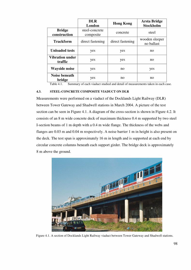
98
DLR
London Hong Kong
Arsta Bridge
Stockholm
Bridge
construction
steel-concrete composite
concrete steel
Trackform direct fastening direct fastening wooden sleeper
no ballast
Unloaded tests yes yes no
Vibration under
traffic yes yes no
Wayside noise yes no yes
Noise beneath
bridge yes no no
Table 4.1. Summary of each viaduct studied and detail of measurements taken in each case.
4.3. STEEL-CONCRETE COMPOSITE VIADUCT ON DLR
Measurements were performed on a viaduct of the Docklands Light Railway (DLR)
between Tower Gateway and Shadwell stations in March 2004. A picture of the test
section can be seen in Figure 4.1. A diagram of the cross-section is shown in Figure 4.2. It
consists of an 8 m wide concrete deck of maximum thickness 0.4 m supported by two steel
I-section beams of 1 m depth with a 0.4 m wide flange. The thickness of the webs and
flanges are 0.03 m and 0.04 m respectively. A noise barrier 1 m in height is also present on
the deck. The test span is approximately 16 m in length and is supported at each end by
circular concrete columns beneath each support girder. The bridge deck is approximately
8 m above the ground.
Figure 4.1. A section of Docklands Light Railway viaduct between Tower Gateway and Shadwell stations.

99
Figure 4.2. A diagram of the viaduct cross-section.
The track form consists of BS80A section rails directly fastened to the concrete deck at
0.6 m intervals with Pandrol baseplates. This baseplate system is a single layer direct
fastening system with a 10 mm resilient rail pad. Both tracks in this location are bi-
directional, and there is a set of points towards the Western side of the measurement span,
so that trains on either track can come to or from Tower Gateway Station or diverge into a
tunnel towards Bank Station.
The rolling stock on the DLR consists of pairs articulated units of types P86/89 or B90/92;
each approximately 14 m in length, with a maximum design speed of 80 km/h (50 mph)
and approximate weight of 38 tonnes (tare).
The mobility at the rail head was measured using the impact hammer technique while no
trains were running to determine stiffness and damping characteristics of the trackform and
to determine the mobility at the rail head for direct comparison with the track models
presented in Chapter 2. Vibration measurements on the rail, and deck were made under
traffic for validation of the SEA part of the bridge model. Simultaneous measurements of
the sound pressure immediately adjacent to the track and underneath the viaduct were
made to validate a full noise prediction of the bridge model.
4.3.1. Measurement method
Unloaded tests. To determine the vertical driving point mobility at the rail head, impact
tests were performed on the viaduct. Two sets of mobility measurements were taken, once
directly above a support and once at a point halfway between two supports. The average of
the two results is then taken.
Measurements under traffic. Ideally, for full validation of the SEA part of the bridge
model, the vibration should be measured on each plate of the bridge. Furthermore, it is

100
desirable to measure the vibration at more than one point on each plate to achieve some
space averaging in the measurements. However, full access to the underside of the viaduct
was not possible meaning that measurements of the vibration of the support girder plates
were not obtained and only deck vibration measurements were made.
Vibration measurements of the deck under traffic were made at two positions along the
span of the viaduct (half-span and quarter-span). The accelerometer positions at each point
on the span are shown in Figure 4.3. Deck vibration was measured at four positions (two at
half-span and two at quarter-span), of which two positions were at the track-centre (a1 and
a2 in Figure 4.3) and two were near the outer edge of the viaduct (a3 and a4). Additionally
rail vibration was measured at the centre of the rail foot of the both rails on one track at
half-span (a5 and a6) for validation of the predicted rail vibration. The accelerometers were
attached to the concrete components in the bridge using an epoxy resin based adhesive and
to the rails using magnetic mounting studs. In both cases the upper frequency limit of
vibration measurements is above 4 kHz.
For validation of the noise prediction from the model, noise measurements were made at
two positions. The microphone positions used are shown in Figure 4.4.
Noise and vibration measurements were made under normal service passenger traffic
between 09:00 and 12:00 during the passage of 48 trains. The morning commuter rush
hour was deliberately avoided to minimise the contribution of commuter traffic on the
nearby roads in the sound recordings. The recordings were made digitally using two DAQ
cards running at a sampling frequency of 12 kHz.
= Accelerometer
a3, a4
8 m
0.03 m
0.4 m
1 m
0.04 m
0.4 m
1 m a1, a2
a5, a6
Figure 4.3. Simplified diagram of the DLR cross section showing vibration measurement positions.

101
7.5 m
1.2 m
1.2 m
8 m
= microphone
microphone boom
M1 - wayside noise
M2 - noise below bridge
Figure 4.4. Microphone positions.
4.3.2. Modelling
4.3.2.1. Input parameters for the rolling stock
The parameters used to model the B90/92 rolling stock are given Appendix A. The train
speed was calculated for all 48 trains from the average time between axle passes seen in
the rail acceleration time histories. The mechanical parameters of the rolling stock were
obtained from DLR. As no wheel or rail roughness measurements were taken in this test,
the wheel roughness used is that typical of disc-braked wheels and obtained using an
energy average of 37 wheel roughness spectra from (Dings and Dittrich 1996) and the rail
roughness is described as an ‘average UK roughness’ (Hardy 1997). The combined wheel-
rail roughness spectrum input to the model is plotted in Appendix A.
4.3.2.2. Input parameters for the track
The rail on this section of DLR is directly fastened to the deck using a baseplate system
with a single layer of resilience. Therefore the rail coupled to the viaduct can be modelled
as two finite Timoshenko beams, representing the rail and support structure, continuously

102
connected by a resilient layer, representing the rail pad (Section 2.3). The parameters used
to define the track and bridge can be found in Appendix A. The rail pad stiffness and
damping has been obtained from the measured mobility (see Section 4.3.3). The
geometrical and material properties of the BS80A rail section were obtained from (Esveld,
1989).
The input mobility of the viaduct. The cross-section of the viaduct consists of a thick
concrete deck stiffened with two steel I-section girders. It is possible that the appropriate
model for the input mobility of the viaduct is either that of a thick concrete plate,
representing the deck, or a steel I-section beam, representing the girders. In practice it is
the ‘stiffer’ of the two components that will dominate the combined mobility of the cross-
section as a complete system and should therefore be used. Figure 4.5 shows the real part
of the driving point mobility of the steel girders modelled as I-section beams. For
frequencies below approximately 700 Hz the beam is modelled using the finite
Timoshenko beam theory presented in Chapter 2 applied to a single beam. For frequencies
above 700 Hz, where the mobility is characterised by in-plane compression of the web and
bending in the flange, the beam is modelled using the theory presented in Sections 3.4 and
3.5. Also plotted in Figure 4.5is the real part of the driving point mobility of the concrete
deck modelled as an infinite thick plate.
In the frequency range 25 Hz to 700 Hz the mobility of the support girders is higher than
that of the concrete deck at most frequencies. The difference is highest at the peaks due to
bending modes of the support girder. However, at the troughs in the mobility of the support
girder this mobility is lower than that of the concrete deck. Furthermore, at many
frequencies there is little difference between the mobility of the two components. As it is
unclear which is the correct model to use in this frequency range, both possibilities have
been tested in the predictions below (Section 4.3.3.2. ).
At 700 Hz a rise in the mobility of the support girder marks the beginning of the high
frequency behaviour of the bridge beam. In the frequency range 700 Hz to 2500 Hz the
mobility of the support girder is consistently higher than that of the deck. However, the rail
is mounted on the deck at a perpendicular distance of 0.47 m from the support girder webs.
Moreover, at approximately 800 Hz one quarter of the bending wavelength of the concrete
deck becomes equal to this distance. Therefore for frequencies above 800 Hz a thick plate
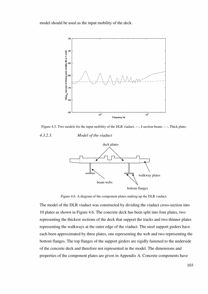
103
model should be used as the input mobility of the deck.
Figure 4.5. Two models for the input mobility of the DLR viaduct. —, I-section beam; – –, Thick plate;
4.3.2.3. Model of the viaduct
deck plates
beam webs
bottom flanges
walkway plates
Figure 4.6. A diagram of the component plates making up the DLR viaduct.
The model of the DLR viaduct was constructed by dividing the viaduct cross-section into
10 plates as shown in Figure 4.6. The concrete deck has been split into four plates, two
representing the thickest sections of the deck that support the tracks and two thinner plates
representing the walkways at the outer edge of the viaduct. The steel support girders have
each been approximated by three plates, one representing the web and two representing the
bottom flanges. The top flanges of the support girders are rigidly fastened to the underside
of the concrete deck and therefore not represented in the model. The dimensions and
properties of the component plates are given in Appendix A. Concrete components have

104
been given a constant loss factor of 0.03 and the steel components have been given
frequency dependent loss factors to describe welded steel (Thompson, Jones & Bewes,
2005).
As discussed in Chapter 1, the assumption of equipartition of energy in the viaduct does
not apply where thick heavy components are connected to thin light components, as the
bending vibration of the low mass component will have little effect on the spatially-
averaged vibration of the high mass component. This is the case for this viaduct, where the
thick concrete deck is connected to the thin steel support girder webs and flanges. The way
of overcoming this that has been chosen here is to place the steel components and concrete
components in separate SEA systems, each of which uses the equipartition assumption.
The system into which the components are placed is important and will depend on the
mobility model used for the viaduct.
If a beam model is used as the input mobility of the viaduct, it follows that the support
girder webs and flanges are placed in a primary SEA system, which receives its power
input from the base of the track. The concrete components are placed in a secondary SEA
system, which receives its power input as an edge-excitation of the concrete deck by the
support girder webs, i.e. the vibration velocity is set as the input assuming that the
receiving subsystem has no effect on the primary SEA system.
Conversely, if a plate model is used, it follows that the concrete components are placed in
the primary SEA system with the support girders in the secondary SEA system. The
secondary SEA system will receive its power input as an edge-excitation of the support
girder webs by the concrete deck.
Due to the location of the rail in relation to the support girder webs, one of the three
models considered for the input mobility of the bridge is a beam at low frequencies and a
plate at high frequencies. For consistency two different SEA models are required to model
the bridge over the full frequency range using this model. This highlights an inadequacy of
the current approach when modelling composite structures such as this viaduct. It is
unclear physically which SEA system should receive the power input from the base of the
track.
For now, three possibilities have been investigated. Firstly, if the beam model used to

105
describe the bridge, the support girders are placed in the primary SEA system (Model A).
Secondly, if the plate model is used to describe the bridge, the concrete components are
placed in the primary SEA system (Model B). The third method investigated is placing the
concrete components in the primary SEA system while using the beam model to describe
the mobility of the bridge (Model C).
4.3.3. Results and model validation.
4.3.3.1. Mobility
Figure 4.7 shows a plot of the magnitude of the driving point mobility at the rail head
measured close to the centre of the viaduct span. Results are presented within the
frequency range 80 to 800 Hz. Signal-to-noise problems prevented measurement of the
mobility outside this frequency range. However this range is adequate for validation of the
track model described in Chapter 2 as the high frequency driving point mobility of rails is
well known and the region where the rail becomes decoupled from the bridge beam is of
most interest for this study. The peak at approximately 310 Hz corresponds to the
decoupling frequency as described in Chapter 2. Also plotted in Figure 4.7 is the spatially-
averaged magnitude of the driving point mobility predicted using the Timoshenko beam
model described in Section 2.3. The material and geometrical properties of the bridge and
rail beams are known, therefore the dynamic stiffness of the rail fastening, s, was
calculated by fitting the peak of the predicted mobility curve to the measured results. This
gave a value of 84 MN/m per fastener. This value of rail pad stiffness can now be input
into the full model and used for the calculation of a complete noise and vibration
calculation.
Between 80 Hz and the decoupling frequency good agreement can be seen between the
measured and predicted mobilities. In this region the rail and bridge motion are becoming
uncoupled. In this region no prominent bending modes in the bridge are seen, suggesting
high damping in the bridge. A frequency dependent loss factor for the bridge that ranges
from 0.3 at 50 Hz to 0.03 at and above 500 Hz has been used in the predictions. For
frequencies above the decoupling frequency and up to 800 Hz the mobility tends towards
that of the rail alone. Although no individual modes can be seen, the peaks and troughs in
the mobility suggest that the finite length of the bridge affects the mobility even at high
frequencies. In this range, agreement between the measured and predicted mobilities is not

106
as good, with the predictions 3 to 5 dB above the measurements between 400 Hz and
600 Hz. The peak in the measured mobility seen at 600 Hz is likely to be the pinned-
pinned frequency of the rail which for a fastener spacing of 0.6 m is expected to occur
around 800 Hz.
Figure 4.7. Magnitude of the driving point mobility of the rail on the DLR viaduct. —, measured at the bridge centre; – –, predicted spatial average.
4.3.3.2. Noise and vibration
The spatially-averaged vibration velocity on the deck has been calculated by averaging the
measured vibration at measurement positions a1 and a2 (Figure 4.2) for all 48 trains. The
same has been done for the vibration on the walkway for measurement positions a3 and a4
and the rail foot vibration at measurement positions a5 and a6. Figure 4.8 shows the
measured deck vibration in one-third octave frequency bands. Also plotted is the range of
measurements recorded. It can be seen that the measured velocity spectrum is dominated
by low frequency components with a velocity level of 90 dB seen at 40 Hz compared with
45 dB at 2.5 kHz.
As discussed in Section 4.3.2, the vibration has been predicted using three different
combinations of bridge mobility and SEA model. These three predictions are also plotted
in Figure 4.8. The prediction using Model A (dashed line) gives poor agreement with
measurement. In the frequency range up to 1600 Hz the model over-predicts the deck

107
vibration by up to 20 dB.
Good agreement is found between the prediction using Model B and the measurement in
the frequency range 100 Hz to 500 Hz. In this range the prediction is within ±1 dB of the
average measured vibration at all frequencies. Below 40 Hz and above 500 Hz the deck
vibration is under-predicted by this model. At approximately 63 Hz a peak is seen in the
predicted vibration that is not seen in the measurements. This corresponds to the natural
frequency of the unsprung mass of the wheel and rail vibrating on the stiffness of the track.
At this mode the vibration of the deck is over-predicted by approximately 10 dB.
The prediction using Model C agrees well with measurement between 100 Hz and 600 Hz,
with errors of no more than 5 dB at discrete frequency bands. However the agreement is
not as good as for Model B. The peak at 63 Hz is much smaller, meaning the prediction of
the deck vibration is much better in the frequency range 50 Hz to 100 Hz. Above 800 Hz
the plate part of the beam-plate model is used for the prediction, yielding the same result as
Model B.
From these results it is not clear if the Model B or Model C model gives the best
representation of the input mobility of the bridge. Comparing the various results it is clear
that the poor result for Model A is not due to the assumption that the bridge behaves like a
beam at low frequencies, but due to the assumption that the deck receives its excitation
from the support girder webs. This model is therefore discounted.
It was shown in Figure 4.5 that, at most frequencies, the mobility of the concrete deck is
less that that of the steel I-section beam. Therefore it is surprising that the use of the plate
model for the bridge mobility at all frequencies should result in a higher vibration of the
deck than using the beam mobility. It can also be seen in Figure 4.5 that for frequencies
below 700 Hz the steel I-section beam is behaving as a Timoshenko beam. Consequently
the power input to the bridge, when the beam mobility model is used, is calculated using
the coupled rail-bridge beam model described in Chapter 2. When the plate mobility model
is used, the coupling between the rail and bridge is not accounted for and the force acting
on the bridge through the fastening system is calculated as if the track is connected to a
rigid foundation. This means that it is likely that this force is artificially high. This would
explain the high magnitude peak seen at the natural frequency of the unsprung mass of the

108
wheel and rail on the stiffness of the track for the case when a plate mobility model is used.
It is also clear that placing the deck and walkways in the primary SEA system while using
the beam mobility model still gives a reasonable result. It is possible that this is due to the
fact that both components make up the stiffness of the bridge and therefore it is not clear
which SEA system the power should be input to. To overcome this problem a more
sophisticated SEA model of the bridge, including the coupling between the impedance
mis-matched components of the bridge, is required for this type of composite structure.
This is outside of the scope of this project and for now it is concluded that the use of the
beam-plate mobility for the bridge while inputting the power into the concrete deck
(Model C) is the best representation of this structure.
Figure 4.8. The spatially-averaged vibration on the bridge deck. —, measured average; , measured range. – –, Model A; •••, Model B; – • –, Model C.
Figure 4.9 shows the spatially-averaged vibration measured on the walkway plates and the
range of measurements recorded. The corresponding walkway vibration prediction using
Model C is also plotted. As for the deck plate vibration, the spectrum is dominated by the
low frequency components. It can be seen that agreement between measurement and
prediction for this case is better than for the deck plate vibration with the model predicting
the walkway vibration well between 50 Hz and 1 kHz. Again the model under-predicts the
vibration at very low frequencies and at very high frequencies.

109
The SEA part of the model works on the assumption that there is a high modal density in
the bridge. At low frequencies this may not be true and therefore the under-prediction of
the deck and walkway vibration for frequencies less than 50 Hz may be partly due to the
lower limit of the SEA assumption being reached. However insufficient measured data was
obtained from the bridge to clarify this.
The under-prediction of the deck and walkway vibration at high frequencies may also be
due to the assumed roughness spectra. Another explanation is that the level of isolation of
the rail from the bridge at high frequencies is not as high as predicted and that the use of a
single frequency-independent value for the dynamic stiffness is an over-simplification.
Figure 4.9. The spatially-averaged vibration on the walkway. —, measured average; – –, predicted; , measured range.
The sound power per unit length predictions for the viaduct and rolling noise have been
converted to a total sound pressure spectrum by considering the sources as incoherent line
sources and accounting for the noise barrier in the wayside noise predictions according to
Maekawa’s formula (Bies and Hansen 2003). Figure 4.10 shows the average A-weighted
sound pressure level measured underneath the viaduct together with the range of
measurements and the predicted sound pressure level radiated by the bridge structure
alone. No account for the wheel-rail noise has been included in the prediction, but it is
expected that shielding from the viaduct deck will mean that the contribution of the wheel-

110
rail noise to the measured noise level will be small. Agreement between the predicted and
measured sound pressure levels is good between 40 Hz and 630 Hz, apart from the 100 Hz
and 125 Hz frequency bands, with predicted levels within ±3 dB of the average measured
levels. Below 40 Hz the model under-predicts the measured sound pressure level in a
similar way to the vibration measurements. Above 630 Hz the predicted sound pressure
level radiated by the bridge structure begins to roll off sharply, while the measured level
peaks at 800 Hz. It was seen from Figure 4.8 and Figure 4.9 that the model under-predicts
the measured deck vibration above 600 Hz and the walkway vibration above 1000 Hz.
Therefore accurate prediction of the sound pressure level radiated by the viaduct at high
frequencies is not expected. Furthermore, although shielded by the bridge deck, a
contribution from the noise from the wheel and rail is expected on the microphone directly
below the viaduct at high frequencies. However the measured sound pressure level below
the viaduct is highest in the frequency range 100 Hz to 800 Hz and the prediction is good
over most of this range. Therefore the model has enabled prediction of the majority of the
important frequency bands in terms of noise radiation from the bridge.
The A-weighted sound pressure level measured 7.5 m from the track centre is plotted in
Figure 4.11 together with the measured range and the sound pressure level predicted using
the model. Also plotted in Figure 4.11 are the predicted structure-radiated component of
the noise and the predicted wheel-rail noise component.
Below 40 Hz the predicted total noise component is much lower than the measured sound
pressure level, as for the case of the noise below the bridge. Again it is due to the under
prediction of the vibration in this range. In the frequency range 40 Hz to 600 Hz,
agreement is better although it is not as good as for the noise measured underneath the
viaduct. In most frequency bands the predicted sound pressure level is within 4 dB of the
average measured sound pressure level.
The contribution to the total sound pressure level from the structure-radiated component
dominates the total sound power up to approximately 500 Hz. Above 500 Hz the total level
remains high as the noise component due to radiation from the wheel-rail dominates the
total level. Due to the inclusion of the wheel-rail noise in the prediction, the agreement is
good between measured and predicted up to approximately 2 kHz. Therefore the under-
prediction of the structural vibration and structure-radiated noise at high frequencies is of

111
less importance when considering the total noise radiated.
Figure 4.10. The sound pressure levels underneath the DLR viaduct. —, measured average; – –, predicted structure-radiated component; , measured range.
Figure 4.11. The wayside sound pressure levels adjacent to the DLR viaduct. —, measured average; – –, predicted total; •••, predicted structure radiated; –▪–, predicted wheel-rail; , measured range.
4.4. MEASUREMENTS ON A CONCRETE VIADUCT IN HONG KONG
Two noise and vibration surveys were performed on a concrete viaduct on a curved section
of the Airport Express (AEL) just outside Chep Lap Kok Airport in Hong Kong.

112
Measurements of deflection and vibration were first made on the existing track form,
which consisted of resilient baseplates on a concrete slab. These measurements were
repeated after the resilient baseplates had been replaced with the Pandrol Vanguard
fastening system. The same rail remained in place throughout and the measurements were
made within a few days of each other. A picture taken approximately 20 m to the east of
the test site can be seen in Figure 4.12. The test installation was 94 m long on a curve of
radius 306 m between kilometre posts 58.673 and 58.777. The installation of Pandrol
Vanguard baseplates was on the ‘up’ track, on the right in Figure 4.12; trains ran from the
west (out of frame to the front) towards Chep Lap Kok airport station (background). The
gradient of the track at the test site is 2.94% uphill and the cant of the track is 120 mm. At
the airport station the up track at the arrivals hall is above the down track at the departures
hall. The test section is on the continuation beyond the airport terminal station to a depot.
Two separate viaducts carry the two tracks from the airport over a road and brown belt
land. The viaducts merge together as the tracks reach the same level.
Figure 4.12. Overhead photograph showing the track and viaduct 20 m to the east of the test site.

113
Figure 4.13. The underside of the viaduct consisting of two concrete box sections supporting the deck.
Figure 4.14. A diagram of the airport viaduct cross section.
Figure 4.13 shows the underside of the viaduct. It is constructed as a concrete trough
supported by two concrete box-sections, one beneath each track, as shown in Figure 4.14.
Cast concrete panels form the sides of the bridge and it has concrete pillars beneath each
box-section supporting the viaduct spans. At the position where the track was
instrumented and the measurements made, the viaduct is approximately 5.2 m wide, and
the instrumented span is approximately 30 m in length.
The existing track form was UIC 60 rail supported in resilient baseplates, fitted with a
10 mm studded rail pad. A 94 m stretch of resilient baseplates between two rail movement
joints was replaced with the Pandrol Vanguard fastening system. The existing UIC 60 rail
was retained. Displacement and vibration measurements were then taken on the new

114
system at the same positions as for the previous tests. A total of 65 Pandrol Vanguard
baseplates were installed on each rail in the first two nights, meaning that the
measurements on the existing track form were made on a 35 m length of resilient baseplate
track that remained. On the third night the remaining fasteners were installed allowing the
measurements on the Pandrol Vanguard system to be made on the full 94 m of track.
4.4.1. Measurement Method
Unloaded tests. As for the DLR viaduct, impact tests were performed to determine the
vertical driving point mobility at the rail head. Impact tests were performed on the low rail
(see Figure 4.14) at the measurement position 6 m from the support column both before
and after the installation. The equipment set-up and procedure was identical to that used
for the unloaded tests on the DLR viaduct (Section 4.3.1).
Measurements under traffic. Vibration measurements were performed on the rail and on
each major component of the cross-section. Where possible, measurements were made at
both the 1 m and 6 m positions. The accelerometer positions are shown in Figure 4.15.
Strain gauge displacement transducers were also used to measure deflections of the rail
relative to the concrete slab; such measurements can be used to accurately obtain the train
speed of a passing train. No sound pressure measurements were made at this site due to the
high level of background noise from a nearby construction site.
Measurements were made between the hours of 0600 and 0900 under normal traffic, which
consists only of MTR Airport Express trains. The signals from 12 trains were recorded on
the resilient baseplate track followed by 11 trains after the installation of Vanguard. The
analogue outputs from the deflection and acceleration measuring equipment were recorded
at a sampling frequency of 12 kHz. The temperature when the vibration and displacement
measurements were made was roughly constant at about 18°C. The weather was fine and
clear for both the ‘before’ and ‘after’ measurements.

115
a1 (6 m)
a2 (6 m)
a3 (6 m) a4, a5 (1 m & 6 m)
a6, a7 (1 m & 6 m)
a8, a9 (1 m & 6 m)
= accelerometer
Figure 4.15. A simplified diagram of the Hong Kong viaduct cross-section showing the vibration measurement positions.
4.4.2. Modelling
4.4.2.1. Input parameters used to define the rolling stock.
The rolling stock on the AEL consists entirely of 7-car AEG-CAF EMU rolling stock. The
parameters used to define the rolling stock were obtained from MTR and are given in
Appendix B. The average train speed was calculated from the rail deflection time history
data and found to be roughly the same on the two measurement days. A typical disc-braked
wheel roughness spectrum (Thompson, Jones & Bewes 2005) has been used to define the
excitation input from the rolling stock.
4.4.2.2. Input parameters used to define the track.
The parameters used for this rail section together with all the parameters used to model the
track are shown in Appendix B. An average UK rail roughness (Hardy 1997) has been used
to define the wear conditions on the rail. Each rail is directly fastened to a concrete slab
with the resilient baseplate or Vanguard fastening system. The dynamic stiffness and loss
factor of 31 MN/m and 0.15 respectively for the resilient baseplate system are calculated
from the mobility measured at the rail head (Section 4.4.3). To model the track after the
installation of Vanguard, these values are replaced with a dynamic stiffness and a loss
factor of 3.3 MN/m and 0.27 respectively which were also obtained from the mobility
measurements.

116
To model the coupling between the rail and bridge up to approximately 600 Hz, an
approximation of an I-section support girder for input to the model described in Chapter 2
is required. The dimensions of the box-section webs are used to form the support girder
webs in the model. An approximation of the flanges of the support girders are constructed
by accounting for the deck that makes up the upper flange of the support girders and the
lower box-flange that makes up the lower flange of the support girder. From these
dimensions an average flange width has been used. These dimensions are also shown in
Appendix B.
4.4.2.3. Input parameters used to define the bridge.
The viaduct is represented by splitting the cross-section into seven plates as shown in
Figure 4.16. The slab supporting the track and the section of deck directly beneath are both
modelled as a single plate, labelled ‘deck’ in Figure 4.16. The dimensions of each plate are
given in Appendix B. The construction material of each plate is concrete.
box webs
bottom flange
walkway
parapet
deck
Figure 4.16. Details of the viaduct cross-section split into component plates for the SEA model.
4.4.3. Results and model validation.
4.4.3.1. Mobility.
The driving point mobility in the frequency range 25 Hz to 600 Hz, measured at the
railhead on the high rail and low rails of the resilient baseplate track are shown in
Figure 4.17 and Figure 4.18. The mobilities measured directly above a fastener and at the
mid-span between two fasteners are both plotted. As for the DLR viaduct, signal-to-noise
problems prevented measurement of the driving point mobility outside of this frequency

117
range. For the high rail, two distinct peaks can be seen in the mobility at approximately
150 Hz and 220 Hz. This suggests that there are inconsistencies in the stiffness of the
fastenings along the high rail as a single peak at 150 Hz is seen for the low rail. From this
more consistent result it can be assumed that for the resilient baseplate track, the rail
decouples from the bridge at approximately 150 Hz.
Also plotted in Figure 4.17 and Figure 4.18 is the spatial average of the predicted driving
point mobility calculated at twenty random points along the span of the bridge. The result
has been ‘tuned’ to the measured mobility by adjusting the values for rail pad stiffness and
rail pad loss factor. For the high and low rails this gave a value for the rail pad stiffness of
31 MN/m. Differences in the sharpness of the peak at the decoupling frequency meant that
values for the loss factor of the rail pads of 0.20 and 0.15 were used for the high and low
rails respectively. It can be seen that, as for the DLR case, the mobility tends to that of the
rail for frequencies above the decoupling frequency and tends towards the combined
mobility of the rail and bridge for frequencies below the decoupling frequency. Other than
the peak seen at 220 Hz on the high rail, agreement is good throughout the full frequency
range in both cases.
For the low rail the mobilities measured above and between the supports differ
substantially at very low frequencies. It is likely that this is due to measurement error in the
mobility measured directly above the support. However apart from this there is little
difference between the measured mobility above and between the supports at most
frequencies in both cases. This confirms that the rail can be modelled as continuously
connected to the bridge for frequencies below the pinned-pinned frequency, which can be
expected to occur at approximately 1 kHz for this case.

118
Figure 4.17. The driving point mobility of the high rail on the resilient baseplate track. —, measured above support - high rail; – –, measured mid-support - high rail; •••, predicted spatial average.
Figure 4.18. The driving point mobility of the low rail on the resilient baseplate track. —, measured above support - low rail; – –, measured mid-support - low rail; •••, predicted spatial average.
The magnitude of the driving point mobility measured at the railhead of the low rail on the
Vanguard track is plotted in Figure 4.19. As for the previous cases, the mobilities
measured above and between the rail fastenings are similar, with slight differences in the
magnitude of individual modes. For this case, a distinct peak is seen at approximately

119
50 Hz. This is the decoupling frequency of the rail from the bridge. Also plotted in
Figure 4.19 is the spatial average of the driving point mobility calculated at 20 random
points along the bridge span. In this case, values for the dynamic stiffness and hysteretic
loss factor of the fastening system of 3.3 MN/m and 0.27 were chosen. A good
approximation of the response in the frequency band surrounding the decoupling frequency
is achieved with these values. In the frequency range 50 Hz to 100 Hz peaks and troughs
can be seen in the measured mobility that are not seen in the prediction. Again it is likely
that this is because individual modes may not be seen in the spatially-averaged mobility.
Above 100 Hz, where the modal density becomes too high to spot individual modes, the
predicted mobility is in good agreement with the measured mobility. Below 50 Hz it is not
clear if the measured mobility is tending to that of the combined mobility of the rail and
bridge beams as the decoupling frequency occurs at a very low frequency relative to the
frequency range measured. However the prediction is in good agreement with
measurement in the range shown.
Figure 4.19. The driving point mobility of the low rail on the Vanguard track. —, measured above support - low rail; – –, measured mid-support - low rail; •••, predicted spatial average.
4.4.3.2. Vibration.
The spatially-averaged vibrations of each bridge plate have been calculated from the
average of the two vibration signals recorded on the each component at both span positions
during the pass by of all twelve trains on the resilient baseplate track. The same has been

120
done for the eleven trains on the Vanguard track. An average of all trains on each track
has been taken. The results for the spatially-averaged vibration velocity on the deck,
averaged over all trains on the resilient baseplate track is plotted in Figure 4.20, together
with the range of levels recorded. Variation of approximately ±3 dB can be seen, even
though the train speed was almost constant. A distinct peak can be seen in the results in the
50 Hz and 63 Hz frequency bands. This corresponds to the natural frequency of the
unsprung mass of the wheel and rail vibrating on the stiffness of the track. Also plotted in
Figure 4.20 are three predictions of the spatially-averaged deck vibration from the model.
Each prediction has been calculated with a different value for the damping loss factor in
the deck plate, 0.3 (dashed line), 0.03, (dash-dot line) and 0.003 (dotted line). Damping of
the concrete deck is unknown and in reality it may be a function of frequency. Predictions
of the spatially-averaged vibration velocity in the deck with three different damping loss
factors suggests that if a frequency dependent damping loss factor varying from 0.3 at
25 Hz and 0.003 at 1000 Hz was used a prediction with increased accuracy over a large
frequency range would be achieved. This would however be a large frequency variation of
damping.
The spatially-averaged vibration on the viaduct walkways averaged for all 12 trains on the
resilient baseplate track, processed in the same manner as for the deck vibration, is plotted
in Figure 4.21. It can be seen that the measured spectrum has a similar shape to the deck
vibration in Figure 4.20 with the low frequencies dominating the spectrum. The peak in the
50 Hz and 63 Hz frequency bands is again seen, with greater prominence than for the case
of the deck. Also plotted in Figure 4.21 are the predictions performed using the same three
damping loss factors for the viaduct walkway. These results suggest that the damping in
the walkway may not be as high as in the deck at low frequencies.
The results for the spatially-averaged vibration measured on the box-section webs are
plotted in Figure 4.22. Again predictions using damping loss factors of 0.3, 0.03 and 0.003
have been performed. Similar results are seen as for the cases of the deck and walkway,
suggesting again that the use of a frequency dependent damping loss factor may be
appropriate.

121
Figure 4.20. The spatially-averaged vibration on the viaduct deck with resilient baseplates. —, measured average;
, measured range; – –, predicted η = 0.3; – • –, predicted η = 0.03; •••, predicted η = 0.003.
Figure 4.21. The spatially-averaged vibration on the viaduct walkway with resilient baseplates. —, measured
average; , measured range; – –, predicted η = 0.3; – • –, predicted η = 0.03; •••, predicted η = 0.003..

122
Figure 4.22. The spatially-averaged vibration on the viaduct box-section webs with resilient baseplates. —,
measured average; , measured range; – –, predicted η = 0.3; – • –, predicted η = 0.03; •••, predicted η = 0.003.
The measured spatially-averaged deck vibration recorded after the installation of Vanguard
baseplates is plotted in Figure 4.23, together with the range of measured results. Firstly the
distinct peak seen in Figure 4.20 in the 50 Hz and 63 Hz frequency bands is not present in
the measurements on the Vanguard track. This is expected, as a reduction in fastener
stiffness by a factor of 10 gives a reduction in track stiffness by a factor of 5.6 and will
lower the frequency at which the resonance of the moving masses of the wheel and rail on
the stiffness of the track occurs by a factor of 2.4.
The predicted deck vibration is also plotted in Figure 4.23. For this prediction the
parameters for Vanguard calculated from the mobility measurements have been used and a
loss factor of 0.03 has been used for the deck. The prediction for the resilient baseplate
track with this loss factor agreed best with measurement in the frequency range 80 Hz to
300 Hz. It can be seen that this is not the case for the Vanguard track. The vibration of the
deck is under-predicted by up to 30 dB in this range. The extent of the under-prediction is
so great using the model that it is clear that the use of a frequency dependent loss factor for
the bridge deck would have little effect on the agreement. The large discrepancy of the
prediction for the Vanguard track using the same rolling stock, bridge and rail parameters
as for the resilient baseplate track, suggests that some additional means of power transfer

123
from the rail to bridge is present for the Vanguard case that is not accounted for in the
current modelling method.
Figure 4.23. The spatially-averaged vibration on the viaduct deck with Vanguard baseplates. —, measured
average; , measured range; – –, predicted η = 0.03.
Figure 4.24 shows the measured insertion loss on the deck due to installing softer
baseplates on the viaduct together with the insertion loss predicted using the model. The
insertion loss is calculated by subtracting the vibration level of the deck in each frequency
band after the installation of the Vanguard baseplates from the corresponding levels for the
resilient baseplate track. Hence positive values indicate a reduction of vibration in that
frequency band. In the measured insertion loss, reduced deck vibration is seen with
Vanguard baseplates between 30 Hz and 500 Hz. The reduction in vibration is greatest
between 40 Hz and 80 Hz. This is due to the lower resonance frequency of the wheel and
rail on the stiffness of the fastening system. For frequencies above 600 Hz, negative values
of insertion loss show an increase in vibration on the deck with Vanguard. The predicted
insertion loss again shows reduced vibration on the deck above approximately 30 Hz.
However the predicted insertion loss rises much more rapidly between 30 Hz and 50 Hz
than for the measurement. Furthermore the prediction remains roughly constant at 20 dB
above 50 Hz. This is expected, as the dynamic stiffness of the fastening system is
approximately a factor of 10 (20 dB) softer than the resilient baseplate system and this is
the only parameter that was altered in the model. According to the theory presented in

124
Chapter 2, a reduction in fastener stiffness will result in a reduction in deck vibration above
the decoupling frequency of the rail from the viaduct. To obtain an increase in vibration in
a frequency band higher than the decoupling frequency, as seen in the measurements,
transmission effects not accounted for in the model must be occurring in practice. Two
possible reasons for this could be:
1. Frequency or load-dependent dynamic stiffness of the fastening system. The
dynamic stiffness of the fastening system in each case has been calculated by curve fitting
to the measured mobility at the rail head in unloaded conditions. The dynamic stiffness of
the fastening system will increase under the load of the rolling stock. It is possible that the
increase in the Vanguard dynamic stiffness will be greater than for the resilient baseplate
system. Also the method used to calculate the dynamic stiffness of the fastening system
means that only a single value for the dynamic stiffness at a single frequency can be
extracted from the mobility measurements. It is known that the dynamic stiffness of
resilient elements varies with frequency partly due to the internal modes of vibration,
which are seen as a peak in the dynamic stiffness of the baseplate. Due to the relatively
large thickness of the resilient elements in the Vanguard system, it is possible that the
increase with frequency in the Vanguard system is much higher than for the resilient
baseplate system. Although this possibility requires further investigation, very little
frequency and load-dependent dynamic stiffness data exists for Vanguard baseplates and
from the results shown in Figure 4.24 very large differences in the dynamic stiffness due to
load and frequency would be required to model correctly the insertion loss. For these
reasons this effect is not investigated further here.
2. Neglect of the lateral forces acting on the viaduct. Firstly the viaduct supports a
curved track, which may result in higher lateral forces acting on the deck than on a viaduct
supporting straight track. Secondly, due to the geometry of the Vanguard system, the rail is
supported beneath the head rather than at the foot. This is designed to give a relatively high
lateral stiffness of the system to reduce lateral and roll movement of the rail. Hence the
lateral forces acting on the viaduct deck may be too large to neglect. This possibility is
investigated in the next section.

125
Figure 4.24. The insertion loss in dB obtained on the viaduct deck from installation of soft baseplates. —, measured average; – –, predicted.
4.4.3.3. Assessment of lateral forces acting on the viaduct
The lateral forces acting on the bridge deck are assessed below. From this, the power input
to the deck laterally is estimated and compared with the vertical power input.
In the same way that the vertical stiffness of the fastening system can be calculated using
the resonance method from the vertical driving point mobility measured at the rail head,
the lateral stiffness can be calculated from the lateral driving point mobility measured at
the rail head. Although not presented in Section 4.4.3.1, measurements of the lateral
driving point mobility at the rail head on the original resilient baseplate track and
Vanguard track were taken. From these measurements the lateral dynamic stiffness has
been calculated using the resonance method. The results are shown in Table 4.2 together
with the values for the vertical dynamic stiffness of each fastening system measured in
Section 4.4.3.1. and the ratios of lateral to vertical stiffness. It can be seen that the resilient
baseplate system is approximately 40 % softer laterally than it is vertically. Conversely the
Vanguard system is 40 % stiffer laterally than it is vertically. This suggests that for the
same vibration of the rail, when translated into forcing on the deck through the fastening
system, the contribution from the lateral direction will be much higher with the Vanguard
system.

126
A diagram of how the deck may be excited from lateral excitation of the rail is shown in
Figure 4.25. A lateral displacement of the rail xL acting on the lateral stiffness KL of the
resilient fastening system results in a lateral force on the deck. The force acts at a
perpendicular distance d from the central axis of the deck, thus exciting it with a moment
M.
Resilient baseplate system
Vanguard system
Vertical stiffness MN/m 31.2 3.3
Lateral stiffness MN/m 18.5 4.7
Ratio of lateral to vertical stiffness 0.59 1.42 Table 4.2. The vertical and lateral dynamic stiffness of the two fastening systems measured on the
Hong Kong viaduct.
xL
d
M
Deck
KL
Figure 4.25. Diagram showing how the deck is forced by lateral excitation of the rail.
In the model, the power input to the deck is considered in the vertical direction alone and is
calculated from the force acting through the resilient fastening system below the wheel into
the deck modelled as either a plate or beam. An approximation of the lateral power input
can be calculated from the measured spatially-averaged lateral acceleration of the rail
webs, also measured on both tracks at this site. The spatially-averaged lateral displacement
of the rail is calculated by integrating the measured spatially-averaged rail web
acceleration twice. This in turn is used to calculate an approximation8 of the lateral force
acting on the deck by multiplying it by the lateral stiffness of the fastening system. In the
model the force at the contact point is multiplied by the real part of the vertical driving
point mobility of the deck. For the lateral case, the deck is excited by a moment. The real
part of the driving point moment mobility of an infinite plate is given by (Cremer, Heckl
and Ungar 1986) as
8 The modelling method calculates the force acting on the deck using vibration of the rail at the contact point
acting on the fastener stiffness. This cannot be measured directly on site and as the decay rates in the rails are
unknown cannot be obtained indirectly from the measurements of rail vibration during a train pass-by.

127
( )32
8.4Re
hc
fW
L ρ= (4.1)
where cL is the longitudinal wave speed in the deck, h is the thickness of the deck and f is
the frequency. Hence the power input to the deck due to lateral forcing of the rail can be
found from equation (2.33) as
( )WxKdP LLlat Re222
21= (4.2)
where 2
Lx is the measured spatially-averaged lateral rail web displacement. Using the
measured spatially-averaged vertical rail foot displacement Vx , a similar approximation
of the power input to the deck due to vertical forcing of the rail from equation (2.33) can
be written as
( )plVVvert YxKP Re22
21= (4.3)
where Kv in the vertical dynamic stiffness of the fastening system in Table 4.2 and Ypl is
the vertical driving point mobility of a thick plate (Cremer, Heckl and Ungar, 1986). The
approximations of the power input due to vertical and lateral forces on the rail in equations
(4.2) and (4.3) have been calculated for each track system using the measured spatially-
averaged rail vibrations and the dynamic stiffness presented in Table 4.2. From these
results the ratio of lateral to vertical power input has been estimated and this is plotted for
each fastening system in dB in Figure 4.26. Positive values of this ratio indicate that the
power input due to lateral forces is larger than the power input due to vertical forces in the
corresponding frequency band.
For the resilient baseplate system, over most of the frequency range the lateral forces are
negligible. For the Vanguard system, the ratio is close to 0 dB above 60 Hz indicating that
lateral force cannot be neglected. At high frequencies power from the lateral vibration is as
much as 8 dB greater than the vertical input. However these results are not sufficient to
explain fully the differences in insertion loss in Figure 4.24.

128
Figure 4.26. The ratio of lateral to vertical power input to the viaduct deck. —, resilient baseplate system; – –, Vanguard fastening system.
4.5. MEASUREMENTS ON A STEEL RAILWAY BRIDGE IN SWEDEN
This section describes a noise survey on the old Arsta Bridge in Stockholm in October
2004. The Arsta Bridge was opened to traffic in 1929, and is on what is now the main
railway route running south from Stockholm Central Station. A newer bridge with the
same name is being constructed parallel to the existing bridge. A diagram of the bridge
span can be seen in Figure 4.27. The bridge is approximately 650 m long and carries two
tracks. The track is approximately 30 m above the water. It consists of a reinforced
concrete arch viaduct section with a short lifting span towards the northern end (now fixed
in position) and a 150 m riveted steel structure towards the southern end where the bridge
crosses the shipping channel. Pictures of the concrete and steel sections can be seen in
Figure 4.28 and Figure 4.29 respectively. The track on the concrete section is ballasted.
The lifting bridge and the steel bridge sections have open deck structures with transverse
timber bearers. The running rails are BV50 section, fixed with Heyback fastenings on
rolled steel plates. Wayside noise measurements were made approximately 40 m away
from this bridge under normal service traffic. The microphone positions were set up on the
new bridge under construction which runs parallel to the west of the old bridge.
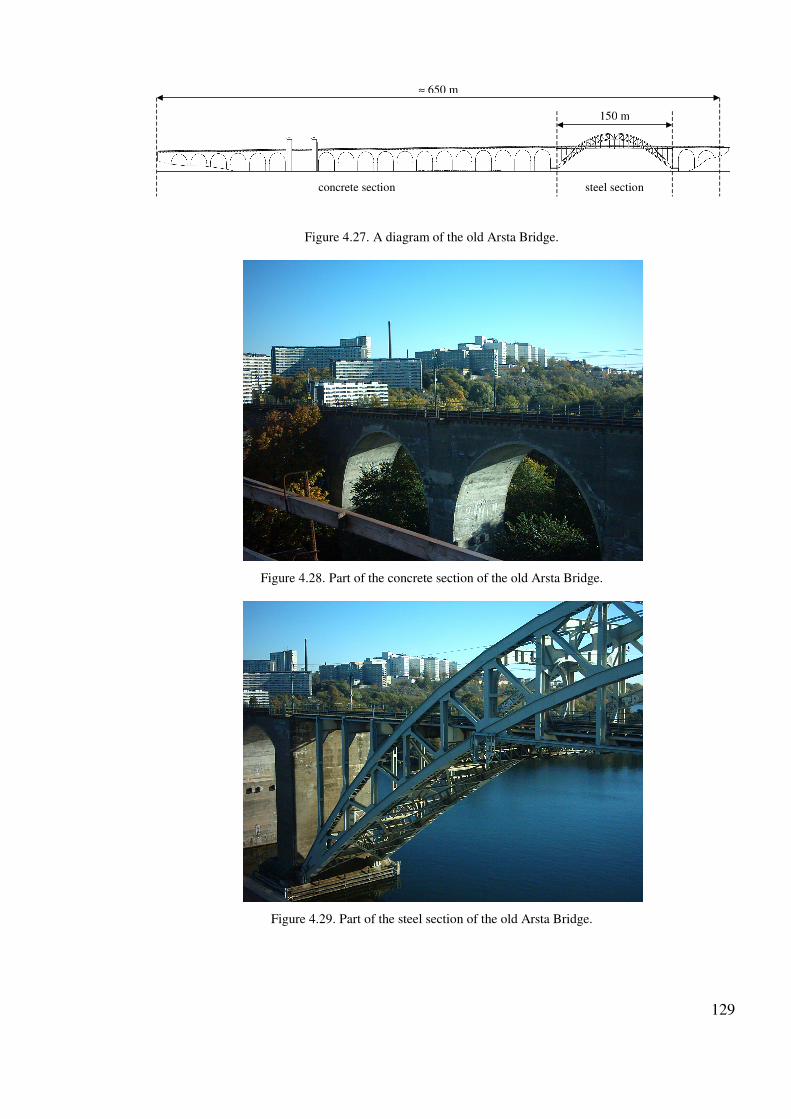
129
≈ 650 m
150 m
concrete section steel section
Figure 4.27. A diagram of the old Arsta Bridge.
Figure 4.28. Part of the concrete section of the old Arsta Bridge.
Figure 4.29. Part of the steel section of the old Arsta Bridge.

130
4.5.1. Measurement method
No track access was granted for this noise survey. For this reason only wayside noise
measurements under traffic were made. Noise was recorded at three positions opposite the
centres of the three different sections of the old bridge: M1 opposite the concrete section
over the water, M2 opposite the concrete section over land on the island and M3 opposite
the steel section over the water as shown in Figure 4.30. In each case the microphone was
positioned on the new bridge at approximately 1.5 m above rail head level. The weather
was fine and clear with no wind and the temperature was between 5˚C and 7˚C when the
measurements were made.
Figure 4.30. Plan view of the old and new Arsta bridges showing the wayside noise measurement positions.
4.5.2. Modelling
It is assumed that the noise radiated by the massive concrete arch sections is low compared
with the wheel and rail noise. Therefore only full noise predictions of the steel section of
the bridge were performed. The parameters used as inputs for the model are presented in
the following sub-sections.
4.5.2.1. Input parameters for rolling stock
Traffic on the day of measurements consisted of various commuter trains made up of 4 to 8
carriages. Data was not available for every type of train crossing the bridge. However one
of the most common types of rolling stock passing over the bridge is the SJ X2000. The
rolling stock parameters corresponding to these trains were obtained from Banverket and
are presented in Appendix C.
The rail or wheel roughness at the site is unknown. An assumed combined wheel/rail
roughness spectrum at 100 km/h is shown in Appendix C, based on typical disc braked

131
wheels and rail roughness in the Netherlands obtained from (Dings & Dittrich 1996)9. The
typical speed of trains passing over the Arsta Bridge has been assumed as 70 km/h.
4.5.2.2. Parameters used to define the track.
The Arsta Bridge supports two tracks. On each track the running rails are BV50 section
fastened to wooden sleepers. On the steel section of the bridge, each sleeper is fastened
directly to two steel I-section support girders. Consequently the sleepers have not been
included in the track model and have been accounted for as a radiating source by
modelling them in the bridge model. It has therefore been assumed that the rail is coupled
to the track support girders (modelled as beams) via the combined resilience of the
unspecified rail pad and wooden sleeper. The dynamic stiffness of the pad in series with
the sleeper has been given a value of 265 MN/m which is typical of stiff pad/wooden
sleeper assemblies (Thompson and Verheij, 1996). Due to the relatively large depth of the
sleepers compared with a conventional rail pad, internal mode effects have been included
in the model of the sleeper stiffness making it frequency dependent. All the track
parameters used for this case are shown in Appendix C.
4.5.2.3. Parameters used to define the bridge.
A detailed drawing of the construction of the steel section of the bridge is shown in
Appendix C. From this and other drawings it has been estimated that the bridge is made up
of approximately 2400 plates. Each of these plates has been grouped by type common to
each cross-section and the dimensions and number of each plate are also shown in
Appendix C. Where the dimensions of a component vary along the length of the bridge an
average length was assumed. The component plates have all been given the properties of
steel. All steel plates have been given a loss factor spectrum which varies from of 0.22 at
10 Hz down to 0.02 at 1 kHz and is equivalent to medium steel damping (Thompson, Jones
and Bewes 2005).
9 This data has been chosen in preference to the UK data of (Hardy 1997) because the grade of steel used in
the UK prior to 1997 is softer than that of the Netherlands and Sweden and so the Netherlands data is more
likely to be representative of the correct wear conditions.

132
4.5.3. Results and model validation
Recordings were made of the noise from 34 trains in total (10 trains at M1, 5 trains at M2
and 9 trains at M3) and recordings with high background noise were eliminated. Between 3
and 5 good quality recordings were identified for each section with similar train type and at
similar speeds. These were then averaged to provide the following results. The average A-
weighted sound pressure level spectra for each train are plotted between 50 Hz and 5 kHz
in Figure 4.31.
The noise measured adjacent to the concrete section over water and the concrete section
over land are similar above approximately 100 Hz. This suggests that the noise measured is
directly radiated wayside noise and that any difference because of a possible component
reflected from the land or water beneath the bridge is negligible.
The noise levels measured adjacent to the steel section are more than 5 dB higher than for
the concrete sections between 50 Hz and 800 Hz. This suggests a significant increase in
structure-radiated noise in this range due to the presence of the steel structure.
Above 1 kHz, the spectra recorded on all three bridge sections are similar. The noise in this
frequency range is likely to be dominated by airborne rolling noise from wheels and rails
which should not depend significantly on the structure beneath the track at these
frequencies.
Assuming that the noise levels radiated by the massive concrete arched sections can be
neglected and that the rolling noise is the same in each case, the component of noise
radiated by the steel structure alone can be estimated by subtracting the concrete section
spectra from the steel section spectra. This result is also plotted in Figure 4.31. This
suggests that on the steel section, the structure-radiated noise is the dominant noise source
in the range 50 Hz to 800 Hz and above 800 Hz the rolling noise is the dominant noise
source. Above 1.25 kHz the estimate of structure-radiated noise is unreliable.
The predictions of viaduct and rolling noise are shown as a sound pressure spectrum for
the steel bridge section in Figure 4.32 along with the measured noise. The prediction is
within ±3 dB of the measured spectrum in all frequency bands between 80 Hz and 4 kHz
except at 630 Hz.

133
Figure 4.33 shows the predicted structure-radiated noise of the steel section and the
estimated structure-radiated component calculated from subtracting the measured noise
levels on the concrete bridge from those on the steel bridge. Predicted levels are within
±3 dB(A) of the estimated noise component in most frequency bands between 80 Hz and
1.25 kHz.
Figure 4.31. The average wayside sound pressure levels measured adjacent to old Arsta Bridge. —, M1 concrete section over water; – –, M2 concrete section over land; •••, M3 steel section over water; – • –, Estimated
noise component radiated by the steel bridge.

134
Figure 4.32. The wayside sound pressure levels adjacent to the steel section of Arsta Bridge. —, measured total = 81.4 dB(A); – –, predicted total = 80.2 dB(A); , measured range.
Figure 4.33. The structure-radiated sound pressure level adjacent to the steel section of Arsta Bridge. —, measured total = 79.4 dB(A); – –, predicted total = 78.8 dB(A).
4.6. SUMMARY
Noise and vibration surveys have been performed on three working railway bridges, in one
case with two track forms. For each case, the rail head mobility, vibration and noise has
been predicted using the bridge noise model described in the previous chapters.

135
On the steel-concrete composite viaduct and for both track types on the all-concrete
viaduct rail head mobility was measured. The data was compared with the predicted
mobility calculated using the coupled rail-bridge beam model described in Chapter 2. For
each of the three cases the mobility was accurately modelled up to the pinned-pinned
frequency of the rail.
For the case of the steel-concrete composite viaduct, uncertainty in the choice of model of
the bridge mobility and SEA representation of the bridge was investigated. It was found
that the use of a beam model for the mobility of the bridge, which accounted for coupling
between the rail and bridge, at low frequencies gave the best representation of the bridge.
However it is still unclear the best way to represent the bridge in the SEA part of the
model. It was concluded that to model a composite structure a more sophisticated SEA
model of the bridge, that includes a more accurate representation of the coupling between
components is required.
Using the beam representation of the bridge below 800 Hz, the model was found to predict
the structural vibration of the concrete components of the steel-concrete viaduct with
reasonable accuracy up to approximately 1 kHz. At high frequencies the model under-
predicts the vibration of each bridge component. It is thought that this is partly due to the
inaccuracy of using a frequency independent dynamic stiffness for the resilient fastening
system. However a large variation of the stiffness would be required to improve the
prediction. This therefore suggests that, at high frequencies, a means of power transfer
from the rail to the bridge, not accounted for in the current model, is present on the track-
bridge system.
Prediction of the noise underneath the viaduct was accurate up to approximately 600 Hz.
Due to the discrepancies between the measured and predicted structural vibration of the
viaduct, good agreement between measured and predicted noise beneath the bridge up to
higher frequencies was not expected. However prediction of the total wayside noise up to
approximately 2 kHz was achieved with the inclusion of the wheel-rail noise component in
the total.
For the case of the all-concrete viaduct, agreement between the measured and predicted
structural vibration of the components in the viaduct for two track types was not as good as
for the case of the steel-concrete composite viaduct. The structural vibration of the bridge

136
was predicted well up to 400 Hz in some cases for the resilient baseplate track. It was
shown that the model is particularly sensitive to structural damping and that improved
results could be obtained if frequency dependent loss factors are used in the model. This
also highlights the importance of obtaining measured damping data for use in the model.
Agreement between the predicted and measured structural vibration of the viaduct with the
Pandrol Vanguard track is poor at most frequencies. It is clear that, in this case, the power
transfer from the rail to the bridge is not correctly modelled using the current method. An
attempt has been made to assess the level of power input to the viaduct from lateral
vibration of the rail. It was shown that this could account for some of the discrepancy
between measurement and prediction with a vertically soft, laterally stiff fastening system
such as Vanguard. However more detailed data is required to quantify this effect more
reliably.
On the all-steel bridge, only wayside noise measurements were made. Agreement between
predicted and measured wayside noise is good up to approximately 4 kHz. The all-steel
bridge is a large structure with relatively low structural damping throughout. Therefore out
of all of the three bridge cases, this bridge is the most suited to the method of modelling
using the SEA approach with the equipartition of energy.
137
5. THE EFFECT ON NOISE OF VARYING CERTAIN
BRIDGE DESIGN PARAMETERS
5.1. INTRODUCTON
5.1.1. Purpose of parameter study
The importance railway bridge noise and vibration knowledge was discussed in Chapter 1.
It was also discussed that Pandrol’s primary method of developing knowledge of the
problem is experimental. In practice noise and vibrations surveys are costly, can take days
to complete and weeks to plan. This means that it is impossible to study the effect of
incrementally varying many bridge noise parameters in this way. However, such a
parametric study would be of great value to Pandrol as it would allow the effectiveness of
many different techniques in reducing bridge noise to be evaluated and the parameters in
the model of most importance to bridge noise to be identified.
Due to the rapid nature of the model developed in Chapters 2 to 4, it is possible to perform
many bridge noise predictions in minutes. For these reasons a study into the effect of
varying certain parameters is conducted in this chapter.
5.1.2. Parameters that affect the noise radiated by a bridge
Figure 1.1 in Chapter 1 showed the three main steps that lead to the noise radiation from a
bridge. The input excitation comes from the wheel-rail roughness causing the rail to
vibrate. Power is then transmitted through the track and into the bridge structure. The
energy then flows throughout the bridge structure causing it to vibrate and ultimately
radiate sound. On this basis, parameters that affect the total noise radiated can be changed
at each stage of the process.
The rolling stock parameters, the wheel-rail roughness and the train speed affect the input
excitation to the track/bridge system. In order to change the power transmission from the
rail to the bridge, the dynamic stiffness of the fastening system can be varied. The input
mobility of the bridge structure also affects the power input to the bridge. Parameters that
then affect the noise radiation from the bridge are the mass, damping and radiation

138
efficiency of the bridge structure.
Each of the above parameters has been varied in the study that is divided into two sections.
In the first section, only changes of the bridge structure are examined and in the second
section, only parameters of the track and input excitation have been varied.
5.2. THE BRIDGES
Three bridge types have been chosen on which to perform the study. The cross-sections of
each type are based on existing bridges. They represent three types of bridge that Pandrol
are frequently asked to provide fastening systems for an all-concrete construction, a steel-
concrete composite construction and an all-steel construction.
It was seen in Chapter 4 that a number of simplifications and assumptions were required to
describe the bridge in the model. For this reason each of the three bridges has an
‘idealised’ cross-section based on an existing bridge of its type. Use of the beam mobility
model of the bridge input described in Chapter 4 has been applied in each case. The rail is
assumed to be mounted directly above the vertical web of the support structure on each
bridge type. This has been done to allow easy comparison of the relative performance of
each type of bridge. It has also been found to be ‘best practice’ when designing a bridge
(Harrison, Thompson & Jones 2000). Again, in the interest of ease of comparison, each
bridge has been given the same length, 30 m.
5.2.1. All-concrete viaduct.
The cross-section chosen for the all-concrete viaduct is based on the viaduct on which
measurements were performed in Hong Kong (Section 4.3) and is shown in Figure 5.1.
The viaduct consists of a 5 m wide deck supported by a concrete box section. It has
parapets at each edge that are 2 m in height and act as noise barriers. The viaduct supports
a single track. Like the Hong Kong viaduct, the bridge can be divided into 8 component
plates for the bridge model. The dimensions and numbers of each plate are shown in
Table 5.1. Each of the component plates has a similar thickness and density. This means
that the equipartition of energy assumption is valid as the components are well matched in
terms of their bending wave impedance. All of the components are therefore in the same
SEA system in the model.
For the calculation of the power input to the bridge, the bridge is modelled as an I-section

139
beam throughout the full frequency range as the rail is assumed to be mounted directly
above the box-section web. The assumed dimensions of the equivalent I-section beam are
1.5 m × 0.5 m for the web and 1.5 m × 0.3 m for the flange. The concrete has been given a
damping loss factor of 0.03.
parapets
deck
walkway
box webs
bottom flange Figure 5.1. Cross-section diagram of the all-concrete construction viaduct used in the study.
Plate component Thickness (m) Width/depth (m) Length (m) Number
Deck 0.5 2.5 30 1
Box webs 0.5 1.5 30 2
Bottom flange 0.3 1 30 1
Walkway 0.3 1 30 2
Parapet 0.3 2 30 1 Table 5.1. Dimensions and number of each plate in the all-concrete viaduct.
5.2.2. Steel-concrete composite viaduct
The second bridge to be studied is based on the steel-concrete composite viaduct on DLR
(Section 4.2). A diagram of the viaduct is shown in Figure 5.2. The cross-section consists
of a 5 m wide concrete deck supported by two steel I-section beams. On the viaduct
studied in Section 4.2, the deck supported two tracks. Here, for simplicity, the deck only
supports one track.
For the case of the DLR viaduct, it was found that the mobilities of the concrete deck and
steel I-section girders were similar. This made it difficult to establish the correct model of
the input mobility of the bridge. The thickness of the deck has been reduced from 0.4 m to
0.25 m in this example viaduct, to ensure that the mobility of the I-section girders is
consistently lower than that of the concrete deck. Therefore, for the power input
calculation, the bridge is modelled as an I-section beam with dimensions as used for the

140
SEA model (Table 5.2). This ensures that the effect of the coupling between the rail and
bridge is accounted for in the frequency range where the bridge beam behaves as a
Timoshenko beam.
The viaduct has again been divided into 8 component plates, the dimensions, number and
construction material of each being given in Table 5.2. Concrete plates have been given a
constant damping loss factor of 0.03. Steel plates have been given a frequency-dependent
damping loss factor (Thompson, Jones & Bewes, 2005).
As for Model C for the DLR viaduct (Section 4.3.2), the deck and walkways are placed in
the primary SEA system and the support girders in a secondary SEA system. The power
from the base of the track is input to the deck and the support girders receive their power
from an edge-excitation of the support girder webs by the concrete deck. However the
results obtained with this approach must be treated with some caution, as the applicability
of the method is unproven.
deck walkways
girder webs
girder flanges
Figure 5.2. Cross-section diagram of the steel-concrete composite viaduct used in the study.
Plate component
Thickness m Width/Depth m
Length m Material Number
Deck plates 0.25 3 30 concrete 1
Walkways 0.25 1 30 concrete 2
Beam webs 0.03 1 30 steel 2
Beam flanges 0.04 0.2 30 steel 4 Table 5.2. Dimensions and properties of the component plates of the steel-concrete composite viaduct.
5.2.3. All-steel steel bridge
The third bridge to be studied is based on an all-steel bridge typically found on many
railway systems in the UK. A diagram of the cross-section is shown in Figure 5.3. The
bridge is approximately 8 m wide and supports two tracks. The cross-section consists of a
thin steel deck supported by four steel I-section beams (one beneath each rail). The bridge

141
has two steel parapets at its edges. The dimensions and numbers of each plate used for the
SEA model are given in Table 5.3. Each plate is constructed from steel. A frequency
dependent loss factor typical of medium damped steel has been used (Thompson, Jones &
Bewes 2005). For the power input calculation, the bridge is modelled as a beam with the
dimensions of the support girders shown in Table 5.3.
As for the all-concrete viaduct, equipartition of energy throughout the whole bridge
structure has been assumed.
deck
support girders
parapets
Figure 5.3. A diagram of the all-steel viaduct used in the study
Plate component Thickness m
Width/Depth m
Length m Number
Deck plate 0.01 7.5 30 1
Support girder webs 0.01 1 30 4
Parapet webs 0.02 3 30 2
Flanges 0.02 0.2 30 16 Table 5.3. Dimensions and properties of the component plates of the all-steel viaduct.
5.3. THE TRACK AND ROLLING STOCK
To allow a direct comparison between the three bridge types all parameters for the rolling
stock have been kept the same. The rolling stock parameters have been chosen to represent
the AEG-CAF EMU rolling stock that was seen on the Hong Kong tests. These parameters
are presented in Appendix B. This train type was chosen as it represents typical light transit
rolling stock that would be compatible with any of the bridges. The only rolling stock
parameter to be varied during the study is the train speed. Predictions for each bridge have
been made for trains running at 40 km/h, 80 km/h and 160 km/h.
A UIC 60 rail section has been used for all cases. This is used in many countries around

142
the world. A direct fastening system has been used to represent the trackform on each
bridge. Although, in practice, ballasted and floating slab trackforms are often used on
bridges, little work has been done in this thesis regarding these trackforms and it was
decided only to investigate the effect of varying the type of direct fastening system used.
The value of the dynamic stiffness of the resilient fastening has been varied in the study.
Six values have been chosen and are shown in Table 5.4. These represent a range from a
very soft fastening system similar to Pandrol Vanguard to a very stiff 5 mm EVA rail pad.
The hysteretic damping loss factor used for each pad in the study has been kept constant at
0.1. In practice it is likely that this value will vary slightly. A higher damping loss factor is
expected in the ‘softest’ fastening systems and a lower one in the stiffest fastening system.
However, for simplicity, only a single parameter has been varied between each prediction.
To study the effect of varying the excitation input to the system, the combined roughness
input used in the model can be changed. This can be done by changing either the rail
roughness or the wheel roughness. Some typical roughness spectra are presented in
(Thompson, Jones & Bewes, 2005) showing the variation in wheel roughness due to the
type of braking system on the rolling stock and the variation in rail roughness due to the
wear on the rail. Changing the wheel roughness will only affect the noise radiated by the
bridge for a single train whereas changing the rail roughness by rail grinding will affect the
noise radiated by the bridge for every passing train. Therefore rail maintenance is a more
direct method by which to control the noise radiated by a particular bridge. For these
reasons when investigating the effect of varying the roughness input on the noise radiated
by the bridge, only the rail roughness is varied. The rail roughnesses used are the ‘normal’
and ‘smooth’ rail roughness presented in (Thompson, Jones & Bewes, 2005). The wheel
roughness is kept as the disc-braked roughness presented in (Thompson, Jones & Bewes,
2005) for the entire study.
Dynamic stiffness MN/m
Description
7 A very soft fastener with stiffness similar to Pandrol Vanguard
30 A typical baseplate stiffness similar to Pandrol VIPA
80 A very soft rail pad typical of a Pandrol 10 mm studded pad
160 A soft pad
500 Medium to stiff rail pad
1600 A hard rail pad typical of a 5 mm EVA pad Table 5.4. The values for dynamic stiffness of the resilient fastening system used in the study.

143
5.4. EFFECT OF BRIDGE STRUCTURE ON NOISE RADIATED
A number of different results are presented and compared in this and the next section. The
focus of this study is on factors that affect the noise radiated by the bridge structure, wheel
and rail. Consequently all results presented are in sound power per metre of bridge length
rather than sound pressure level. This allows comparison of different cases without
considering site-specific factors related to noise propagation.
In order to be able to quantify more quickly the effect of changing particular parameters on
the total noise radiated by a bridge, the results presented below are initially left as un-
weighted levels and spectra. The two outputs of the bridge noise model are the structure-
radiated noise and the wheel-rail noise. These are presented as separate sound components.
From the linear modelling approach taken, it is clear that investigation of the effect of
varying speed on each bridge need only be performed for a single fastener stiffness and
investigation into the effect of changing fastener stiffness need only be done at a single
speed, hence reducing the amount of data requiring analysis.
This section is concerned with the effect of the bridge structure alone and only parameters
that change each structure are varied here. Therefore the train speed and fastener dynamic
stiffness have not been changed. A typical fastener stiffness of 80 MN/m and a train speed
of 40 km/h have been used for the calculations in this section.
Figure 5.4 shows the structure-radiated and wheel-rail-radiated sound power per metre
radiated by each bridge in one-third octave bands between 10 Hz and 5 kHz and as the
total sound power radiated over the whole frequency range.
Above approximately 250 Hz the sound power due to the wheel-rail noise is very similar
for each case, with differences of less than 1 dB between each bridge. This is because the
wheel-rail noise is calculated from the rail vibration, which is in turn calculated from the
vertical rail mobility. It was seen in Chapter 2 from the coupled beam model of the track
and bridge that at frequencies above the decoupling frequency of the rail from the bridge
beam, the vertical mobility at the railhead tends to that of the rail beam alone. As the rail
section and rolling stock have been kept the same for each bridge case, the resulting rail
and wheel vibration are expected to be the same.

144
Figure 5.4. The sound power per metre radiated by each viaduct for a train speed of 40 km/h and a fastener
stiffness of 80 MN/m. Structure-radiated noise: —, all-concrete (Bridge 1); – –, steel-concrete composite
(Bridge 2); •••, all-steel (Bridge 3). Wheel-rail noise: –+–, all-concrete; – + –, steel-concrete composite; •+•,
all-steel. Total: , structure-radiated noise; , wheel-rail noise.
Below 250 Hz, some differences in the wheel-rail noise spectra on each bridge are seen
due to differences in the mobility caused by the bridge structure. However these
differences will have negligible effect on the total sound power. Furthermore in terms of
overall level, differences of less than 1 dB occur between rolling noise on the three bridge
types.
It can be seen that the all-concrete viaduct is the ‘quietest’ bridge with a sound power level
of approximately 95 dB radiated by the bridge structure. In terms of these un-weighted
total levels the steel-concrete composite viaduct is the ‘loudest’ bridge. However further
further analysis of the sound power spectra is required to give a better indication of the
relative performance of the three bridges. In terms of spectra the steel-concrete and all-
steel bridges have similar levels between 30 Hz and 500 Hz.
Each bridge has a peak at about 80 Hz, that is relatively independent of bridge structure,
corresponding to the natural frequency at which the unsprung mass of the train vibrates on
the stiffness of the track. This peak is more distinct in relation to the general level of the
spectrum for the all-concrete viaduct and the steel-concrete composite viaduct than for the
all-steel bridge.

145
It must also be noted that above 200 Hz for the all-concrete viaduct, and approximately
500 Hz for the other two bridges the sound power due to wheel-rail noise becomes the
dominant radiating source in each case. Unless noise mitigation is introduced to reduce the
noise radiated by the wheel/rail (including shielding), noise reduction methods aimed at
reducing the bridge noise radiated above these frequencies will have little effect on the
total noise radiated in each case.
The relative performance of each bridge can be directly related to differences in the two
main processes that lead to radiation from the bridge. Firstly, the level of sound power
radiated by each structure is directly related to the amount of power input to the bridge
through the track. The fastener stiffness is the same on each bridge but it is likely that the
characteristics of each different bridge structure result in differing levels of power input to
the bridge itself.
Secondly, the total sound power radiated by the bridge structure is directly related to the
energy flow through the structure and the noise radiation of the components that make up
the bridge section. For example, it is not clear whether a bridge containing many thin steel
components with a low radiation efficiency but high vibration levels or a bridge made up
from a few concrete components with high radiation efficiency and low vibration levels
might be the noisier, especially given the different behaviour at different frequencies.
Figure 5.5 shows the total power input to the bridge structure for each bridge case. In each
case this is highest at 80 Hz, corresponding to the natural frequency of the unsprung mass
of the train vibrating on the stiffness of the track. The power input is lowest for the all-
concrete viaduct over the whole frequency range, except in the 16 Hz frequency band
where there is a distinct peak. Figure 5.6 shows the sound power radiated per metre by
each bridge structure for a unit power injected to the viaduct at the base of the track. In all
frequency bands the sound power radiated by the all-concrete viaduct is the lowest.
Comparing Figure 5.4, Figure 5.5 and Figure 5.6, between 10 Hz and 50 Hz, the power
input to the all-concrete viaduct is much less than the power input to the steel-concrete
composite viaduct whereas the sound powers radiated for a unit input power are similar.
As the total sound power radiated by the all-concrete viaduct is much less than the steel-
concrete viaduct, the difference is clearly dominated by the differing power inputs to the

146
two bridges.
Conversely, between 250 Hz and 5 kHz, significantly larger differences are seen in the
sound power radiated for a unit input power by each viaduct than the differences seen in
the power input. This suggests that at high frequencies, the higher total sound power
radiated by the steel-concrete and all-steel structures are due the differences in the
radiating properties of the structures.
Between 90 Hz and 600 Hz, the performance of the all-steel and steel-concrete viaducts are
similar in both graphs. This suggests that both the power input and the power radiated are
significant factors in the noise performance of the bridges in this mid frequency range.
Figure 5.5. The total power input to the bridge for a train speed of 40 km/h and a fastener stiffness of 80 MN/m.
—, all-concrete; – –, steel-concrete composite; •••, all-steel.

147
Figure 5.6. The total sound power radiated by the bridge for a unit power input. —, all-concrete; – –, steel-
concrete composite; •••, all-steel.
5.4.1. The power input to the bridge structure
The power input to a structure can be calculated from the product of the square of the force
acting on the structure and the real part of the driving point mobility of the structure.
Figure 5.7 shows a plot of the real part of the driving point mobility of each bridge.
In all frequency bands the mobility of the all-concrete viaduct is the lowest, and that of the
all-steel viaduct is the highest. The low mobility of the all-concrete viaduct is due to the
high mass and bending stiffness associated with the thick concrete webs of this cross-
section. The depth of the support girders on the all-steel bridge and the steel-concrete
viaduct is the same. However the thickness of the webs of the steel-concrete composite
viaduct support girders are three times that of the webs of the all-steel bridge and the
flanges on the former bridge are twice the thickness. Hence the mass and bending stiffness
of the bridge beams for the case of the all-steel bridge is much less, resulting in a higher
driving point mobility.
In the 16 Hz frequency band a mode of the all-concrete bridge can be seen and can account
for the increase in power input to the bridge and total sound power radiated by the bridge.
This highlights the importance of including bending modes in the calculation of the
response of the bridge as described in Chapter 2.

148
Between 40 Hz and 100 Hz the mobility of each viaduct remains roughly constant. An
increase in the power input to the bridge and sound power radiated by the structures was
seen in Figure 5.5 and Figure 5.4, corresponding to the natural frequency of the unsprung
mass of the train vibrating on the stiffness of the track. This shows that the maximum
response in the sound power radiated by and power input to each viaduct is due to a peak
in force acting at the base of the track and not due to the mobility of the structure.
In all other bands, an approximate 5 dB increase in mobility leads to a similar increase in
power input to the bridge. It is clear that for all frequencies other than those associated
with the natural frequency of the unsprung mass of the train vibrating on the stiffness of
the track, the power input to each bridge is directly related to its mobility. Hence the sound
power radiated by each bridge can be changed by changing the mobility of the bridge.
Figure 5.7. The input mobility of the bridge. —, all-concrete; – –, steel-concrete composite; •••, all-steel.
Since a more ‘mobile’ bridge will radiate a higher level of sound power it is possible to
alter the design of the support girder with the aim of reducing the sound power radiated.
This can be achieved across a wide frequency range by adding mass and increasing the
bending stiffness of the support girder. For the case of the all-concrete viaduct, the existing
box-section already contain a lot of mass. For this reason it may be impractical to increase
mass and bending stiffness of the all-concrete viaduct further. In a real situation, increasing
the mass and bending stiffness of the steel support girders on the steel-concrete and all-

149
steel structure is more plausible.
Plotted in Figure 5.8 is the real part of the driving point mobility for three different steel
girders. The solid and dashed lines show the result for the all-steel and steel-concrete
bridge respectively. The dotted line is the mobility of a girder that has webs that are three
times as thick as the webs of the steel-concrete viaduct girder and flanges of twice the
thickness. A web thickness of 0.09 m is very thick for a single cast girder, however an
equivalent web thickness could be achieved by replacing the I-section girder with a box-
section girder with two webs of equal thickness.
Figure 5.8. The input mobility of the bridge. —, all-steel bridge; – –, steel-concrete composite; •••, modified
bridge beam.
An additional prediction has been performed for the steel-concrete viaduct, with the girder
parameters changed to those of the low mobility beam shown in Figure 5.8, all other
parameters have been kept the same. In order to examine the effect of changing the bridge
mobility alone, the SEA parameters have not been changed. Note that, changing the
dimensions of the support girder without changing parameters of the SEA model is not
correct in physical terms, as the support girders are also radiators and their radiating
properties will also change.
Figure 5.9 shows the sound power radiated by the steel-concrete composite viaduct in its
original form (solid line) and the sound power radiated by the viaduct with modified

150
support girders (dashed line). The wheel-rail sound power predictions are not shown as
they are independent of the bridge structure.
Replacing the support girders of the viaduct with heavier and stiffer beams has reduced the
noise radiated by the bridge in all frequency bands. In most bands the improvement is more
than 3 dB and is as much as 8 dB in some bands. The total sound power radiated by the
structure is reduced by approximately 2 dB. This corresponds to a drop in the A-weighted
level of approximately 4 dB(A).
Predictions have also been performed on a modified version of the all-steel bridge after the
support girders on the steel bridge have been replaced with girders of the steel-concrete
composite viaduct (dashed line in Figure 5.8). The results are plotted in Figure 5.10.
Between 50 Hz and 80 Hz the sound power radiated by the bridge structure increases by
1 dB to 2 dB after modification of the support girders. Increasing the ‘stiffness’ of the
support girder will result in an increase in the force acting at the base of the track at the
frequency of the unsprung of the train vibrating on the stiffness of the track, hence an
increase in the power input to the bridge and sound power in this frequency region. Overall
however the total sound power radiated has been reduced by approximately 1 dB. This
corresponds to a reduction of 3 dB in the A-weighted total.
These results show that a design change in the structure can be significant in altering the
sound power radiated by the structure. Increasing the web thickness 3-fold and doubling
the thickness of the flange may be considered a reasonable increase in construction cost.

151
Figure 5.9. The sound power per metre radiated by the steel-concrete composite viaduct for a train speed of 40 km/h and a fastener stiffness of 80 MN/m. Structure-radiated noise: —, with original support girders; – –,
with modified support girders. Total: .
Figure 5.10. The sound power per metre radiated by the all-steel bridge for a train speed of 40 km/h and a fastener stiffness of 80 MN/m. Structure-radiated noise: —, with original support girders; – –, with modified
support girders. Total: .
5.4.2. Sound radiation from the bridge structure
In the previous sub-section the relationship between the total sound power radiated by each
viaduct and its total power input at the base of the track has been discussed. Once power

152
has been injected to the structure, the energy is transmitted throughout the structure
resulting in the vibration of each component in the bridge cross-section. Each component
in the cross-section is a radiator of sound and the total sound power radiated by the bridge
is the sum of the sound power radiated by each component. Therefore, factors that control
the energy flow and radiation from each component may be important factors in
controlling the total sound power radiated by the bridge. In the current modelling approach
the sound power radiated by the nth component in the cross-section can be written as
2
00 nnnn vScW σρ= (5.4)
where ρ0 is the density of air, c0 is the speed of sound in air, σn is the radiation efficiency
of component n and Sn is its surface area. Therefore in this section, the component sound
power radiated, component vibration velocity and radiation efficiency are evaluated and
compared independently of changes to the power input to the bridge structure.
Figure 5.11(a) shows the overall sound power radiated per unit input power for each bridge
component of the all-concrete viaduct. The components contributing most to the total
sound power radiated are the parapets. The second ‘noisiest’ components contributing to
the total sound power radiated for a unit input power are the walkways. The bottom flange,
and deck contribute less, the ‘quietest’ components being the box-section webs.
Figure 5.11(b) shows the equivalent results for the steel-concrete composite viaduct. As for
the all-concrete viaduct, it can be seen that the total sound power radiated by the viaduct is
dominated by a single component in all frequency bands, in this case the support girder
webs. The sound power radiated by the deck, walkways and support girder flanges is
sufficiently low for the radiation to have little effect on the total sound power radiated by
the viaduct as a complete system (Figure 5.6). A peak can be seen in the sound power
radiated by the support girder webs at approximately 400 Hz that corresponds to a peak
seen in the total sound power radiated by the viaduct (Figure 5.4).
Figure 5.11(c) shows the results for the all-steel bridge. Unlike the other structures, the
sound power radiated is not dominated by a single component throughout the full
frequency range. Peaks can be seen in the sound power radiated by parapet webs and
flanges at 630 Hz and by the deck and girder webs at 1250 Hz which correspond to peaks

153
in the total sound power radiated by the bridge (Figure 5.4).
Figure 5.12 shows the spatially-averaged mean square vibration velocity 2
iv of each
component per unit input power for each viaduct. The mean square vibration velocity of
each plate in an assemblage of plates is proportional to the reciprocal of the product of its
damping loss factor, density and square of the thickness (Cremer, Heckl and Ungar 1986).
For the parapets, walkways, and bottom flange of the all-concrete viaduct each of these
properties are the same resulting in an identical mean square velocity. This can be seen as
the higher of the two lines in Figure 5.12(a). The same is true for the deck and box-section
webs that share the same density and damping loss factor but have an increased thickness.
For the steel-concrete composite viaduct, Figure 5.12(b), the highest vibration velocity is
seen for the support girder webs in all frequency bands. The mean square vibration
velocities of the concrete deck and walkway are up to 10 dB less than the vibration
velocities of the steel webs and flanges in the bridge. Comparing the vibration velocity of
each component and the total sound power radiated by each component for this case, it can
be seen that at most frequencies the differences in sound power radiated can be accounted
for by the corresponding difference in the mean squared vibration velocity. It can also be
seen that for this case the vibration velocities of the steel components are higher than those
of the concrete components. This a characteristic difference between thin low mass, lightly
damped components, such as the support girder webs and thick high mass, highly damped
components, such as the concrete deck.
For the all-steel bridge, similar results are seen as for the all-concrete viaduct, with
differences plate thickness resulting in different vibration velocity.
Figure 5.13 shows the radiation efficiency of each component for each viaduct case. The
radiation efficiencies of each component σn used in the model are the standard formulae
for plates and beams given in (Beranek and Vér 1992) and by Maidanik (1962).
Comparing the radiation efficiency of the components in each viaduct with the
corresponding overall sound power radiated by each component, it is clear that although
differences exist between the radiation efficiencies of each component, these differences
cannot account for the large broadband differences in sound power level radiated by each
component.

154
Two main characteristics can be identified from Figure 5.13. Firstly, the critical frequency
of thick concrete elements is generally much lower than for the thinner steel elements.
Secondly, below the critical frequency, the radiation efficiency of the steel components is
in general much lower than that of the concrete components. However, the maximum
radiation efficiency of the typical steel elements is much higher than the maximum
radiation efficiency of concrete elements. This means that when the critical frequency of a
steel component occurs, high magnitude peaks will occur in the total sound power radiated
by the bridge, if the component is one of the dominating components in the viaduct.
Figure 5.11. The overall sound power per metre for a unit input power radiated by each bridge component. (a),
all-concrete viaduct; (b), steel-concrete composite viaduct; (c), all-steel bridge.

155
Figure 5.12. The vibration velocity of each plate for a unit power input. (a), all-concrete viaduct; (b), steel-
concrete composite viaduct; (c), all-steel bridge.
Figure 5.13. The radiation efficiency of each component. (a), all-concrete viaduct; (b), steel-concrete composite
viaduct; (c) all-steel bridge.
5.4.3. Effect of varying structural damping
It was shown above that the mean square vibration velocity of each plate controls the
sound power radiated by the bridge structure over a broad frequency range. The spatially
averaged mean square velocity 2
iv of one plate in an assemblage of plates is calculated in

156
the modelling method as (Cremer, Heckl and Ungar 1986)
∑=
n n
niii
ini
h
Sh
Pv
2
2
ρωη
(5.2)
where Pin is the power input to the system, ω is the circular frequency, ρi, ηi and hi are the
density, damping loss factor and thickness of plate i and hn and Sn are the thickness and
surface area of plate n. As the vibration velocity of each plate is proportional to its
structural damping, it is useful to investigate the sensitivity of the model to this parameter.
For each viaduct case, a calculation has been made with two different levels of structural
damping in the component plates, while no other parameters in the model have been
changed. The value for the hysteretic loss factor used in every component in the SEA
model has been replaced with a value equal to one third of the original value and then three
times the original value.
Figure 5.14 shows the sound power radiated per metre by the all-concrete viaduct for three
different values of structural damping. A three-fold reduction in the damping in each
component of the all-concrete viaduct increases the total sound power radiated by
approximately 5 dB and a three-fold increase in the structural damping reduces the sound
power radiated by approximately 5 dB. This suggests that changing damping has a
significant effect on the sound power radiated by the bridge. The same result can be seen in
the spectral result. An identical result, not plotted here, is also found for the all-steel
bridge.

157
Figure 5.14. The sound power per metre radiated by the all-concrete viaduct for a train speed of 40 km/h and a fastener stiffness of 80 MN/m. Structure-radiated noise: —, with one third original loss factors of structural elements; – –, with original loss factors of structural elements; •••, with three times original loss factors of
structural elements; , total.
Figure 5.15 shows the sound power radiated per metre by the steel-concrete composite
viaduct, calculated for three different values of structural damping. A three-fold reduction
in the structural damping of every component in the bridge has resulted in an 8 dB increase
in the total sound power radiated by the structure compared to the original prediction and a
corresponding increase in the structural damping in each component has resulted in a 7 dB
decrease in the total sound power radiated. This suggests that the effect of damping on the
total sound power radiated by the steel-concrete composite viaduct is much more
significant than on the all-concrete viaduct. Furthermore, it suggests that a change in
damping does not affect the total sound power radiated linearly as expected.
Comparing the three spectra on the left hand side of Figure 5.15, it can be seen that
differences in sound power radiated by the structure due to a change in structural damping
are frequency dependent, unlike for the previous viaducts.
In the SEA model of this structure, equipartition of energy does not apply and the steel
support girder webs receive their excitation from the concrete deck, not directly from the
base of the track. This means that the power input to the support girder webs is
proportional to the mean square vibration velocity of the concrete deck. As well as

158
reducing or increasing the mean square velocity of the support girder webs and flanges
directly by 5 dB, by changing their structural damping, a change in the damping of the
concrete deck will result in a further 5 dB change in the vibration velocity of the support
girder webs and flanges. This shows that the sound power radiated per metre by the steel-
concrete viaduct is particularly sensitive to a change in structural damping.
This result must be treated with caution due to the heuristic nature of the model used and
warrants further investigation.
Nevertheless, even from the results for the all-concrete viaduct and the all-steel bridge, it is
clear that if the structural damping of a bridge could be improved, significant reductions in
the sound power radiated by the bridge could be achieved. However, in practice,
significantly altering the damping properties of materials or structural components can be
difficult. Furthermore, of all the parameters used in the prediction of the noise from a
railway bridge, structural damping is the most difficult to measure or predict and little
published data exists that describes the damping of common construction materials. This
study of the sensitivity of the structure-radiated noise to changes in the damping has
highlighted the importance of this parameter in making accurate predictions of the noise
emanating from a railway bridge more so than indicating how damping can be used to
control the noise radiated by the bridge.

159
Figure 5.15. The sound power per metre radiated by the steel-concrete composite viaduct for a train speed of
40 km/h and a fastener stiffness of 80 MN/m. Structure-radiated noise: —, with one third original loss factors of structural elements; – –, with original loss factors of structural elements; •••, with three times original loss
factors of structural elements; , total.
5.4.4. Effect of varying plate thickness
It was shown above that reducing the mean squared velocity of each bridge component by
increasing its damping has a significant effect on the sound power radiated by each
component. From equation (5.2) it can be seen that the mean square spatially-averaged
velocity of each component is proportional to the reciprocal of the square of the thickness
of that component. Therefore it may be possible to reduce the sound power radiated by the
viaduct by tuning the thickness of the components in the bridge. Working on this
hypothesis, an attempt to reduce the sound power radiated per metre by one of the viaducts
is made below.
It was seen that for the case of the all-steel bridge, the total sound power radiated is not
dominated by the radiation from a single bridge component. Therefore to achieve a
significant reduction in the sound power radiated by the all-steel bridge over a large
frequency range, the thickness of many components in the bridge would have to be
adjusted. For the all-concrete and steel-concrete composite viaducts it was shown that the
total sound power is dominated by the radiation of one component, the parapets on the all-
concrete viaduct and the support girder webs on the steel-concrete composite viaduct.

160
It was discussed in section 5.4.1 that increasing the mass by increasing the thickness of a
component in the all-concrete viaduct may be implausible in practice as the all-concrete
viaduct is constructed from components that are relatively thick. However the damping
study on the steel-concrete composite study showed that care must be taken when altering
parameters of a bridge with two SEA systems due to the way the power flow throughout
the structure is modelled. Therefore, although an increase in the mass of components may
be implausible in practice, a study into the effect of changing the thickness of the parapets
on the all-concrete viaduct has been performed below.
Figure 5.16 shows the sound power radiated per metre by the all-concrete viaduct in its
original form and after changing the thickness of the parapets in the SEA part of the model
from 0.3 m to 0.6 m. Increasing the thickness of the parapets has reduced the total sound
power radiated by the viaduct by approximately 2 dB. Spectral differences of up to 2 dB
are found with the largest difference around 100 Hz.
Figure 5.16. The sound power per metre radiated by the all-concrete viaduct for a train speed of 40 km/h and a
fastener stiffness of 80 MN/m. Structure-radiated noise: —, 0.3 m thick parapets; – –, 0.6 m thick parapets; , total.
To explain the results, Figure 5.17 is a plot of the overall sound power radiated by each
component of the all-concrete viaduct for a unit input power after doubling the thickness of
the parapets. Comparing these sound powers with those before modification of the parapets
in Figure 5.11, it can be seen that the overall sound power level radiated by the parapets

161
after modification has dropped by 5 dB. It can also be seen that the shape of the parapet
spectrum has changed after modification indicating that changing the thickness of the
support girder webs has altered the radiation efficiency of this component.
The significant reduction in the sound power radiated by the parapets means that the
walkways are now the dominant radiating component in the bridge. This means that the
benefit of increasing the thickness of the parapets is limited due to the sound power
radiated by other components in the bridge.
Comparing again the sound powers radiated by each component before and after the
modification of the parapets, it can be seen that while the sound power of the parapets has
been reduced, the sound power radiated by the other components has increased by
approximately 1 dB at all frequencies. Considering the term ∑n n
nn
h
Sh
2 in equation (5.2),
altering the thickness of the parapets has changed the ratio of the impedances of the
components in the bridge, resulting in an increase in the mean square spatially averaged
vibration velocity of each component of approximately 1 dB.
This demonstrates that the vibration velocities of each component in the viaduct are
dependent on each other and attempting to tune the thickness of different components in
order to reduce the sound power radiated by the structure is not straightforward. It was
shown in section 5.4.1 for the cases of the steel-concrete composite viaduct and the all-
steel bridge, that increasing the input mobility of a structure by thickening of the support
girder webs reduces the sound power radiated by the structure. This study shows that such
an improvement was achieved because the parameter was only changed in the mobility
model of the viaduct and not the SEA model. From the prediction here it is now known
that these effects could cancel each other out, resulting in reduced benefit from thickening
a component in the bridge.

162
Figure 5.17. The overall sound power per metre radiated by each bridge component on the all-concrete viaduct
for a unit power input after modification of the parapets. —, deck; – –, box-section webs; •••, bottom flange;
–•–, walkway; –+–, parapets.
5.5. EFFECT OF THE TRACK ON TOTAL SOUND POWER RADIATED
Referring again to Figure 1.1, another way to reduce the noise radiated by a bridge
structure is to alter the track form on the bridge or the input to the track. In doing so it is
possible to reduce either the vibration excitation input to the system or the power flow into
the bridge structure. The benefit of mitigation methods that concentrate on the track
structure is that they do not require any major structural design changes to the bridge and
can be applied after the bridge has been constructed as well as in the design stages of the
bridge construction. For these reasons the effect of varying three parameters of the track
have been studied in this section.
5.5.1. Effect of varying fastener stiffness
The first parameter that is considered is the dynamic stiffness of the rail fastening system.
This will affect the level of isolation of the rail from the bridge and hence the power input
to the bridge. Due to the linear modelling approach taken the effect of varying fastener
dynamic stiffness is independent of the train speed. Therefore analysis has only been done
for a train speed of 40 km/h.
Figure 5.18 shows the sound power radiated per metre for the all-concrete viaduct,
calculated with a rail pad dynamic stiffness of 30 MN/m, 80 MN/m and 160 MN/m.

163
Increasing the fastener stiffness from 80 MN/m to 160 MN/m results in a 7 dB increase in
the total structure-radiated noise and a 1.5 dB drop in the total wheel-rail noise. The
corresponding decrease in total structure-radiated noise and increase in total wheel-rail
noise when reducing the fastener stiffness from 80 MN/m to 30 MN/m are 2 dB and 1 dB
respectively. Thus an increase in fastener dynamic stiffness leads to an increase in the
structure-radiated noise and a decrease in the wheel-rail noise. This is expected since, as
the dynamic stiffness of the fastening system is increased, the level of vibration isolation of
the rail from the bridge is reduced, resulting in an increase in the power transmitted away
from the rail and into the bridge.
Comparing the structure-radiated sound power spectra, the most noticeable change in the
spectra is the shift of the natural frequency of the unsprung mass of the wheel and the rail
vibrating on the stiffness of the track, seen at 50 Hz for the 30 MN/m fastener, 63 Hz for
an 80 MN/m fastener and 80 Hz for the 160 MN/m fastener.
Below 30 Hz there is little difference in the structure-radiated spectra, as at low
frequencies the motion of the rail and bridge are well coupled. Above 300 Hz a significant
reduction in structure-radiated sound power is achieved when the fastening system is
reduced as the motion in the rail and bridge has decoupled and better isolation is achieved
with a more resilient fastening system.
Comparing the wheel-rail radiated spectra, a reduction in fastener stiffness results in an
increase in the wheel-rail radiated noise between 100 Hz and 1 kHz. This is expected as at
high frequencies the rail has decoupled from the bridge resulting in reduced decay rate in
the rail and an increased average vibration of the rail for a reduced fastener stiffness.
Plotted in Figure 5.19 are the structure-radiated sound power level spectra calculated for all
six fastener stiffness values presented in Table 5.4. It can be seen that in all cases three
characteristic changes occur when a less resilient fastening system is replaced with a more
resilient fastening system:
1. The natural frequency of the unsprung mass of the wheel and rail vibration is
reduced in frequency. At this frequency on the less resilient track there is an increase in the
structure-radiated sound power.
2. At the natural frequency of the unsprung mass of the wheel and rail on the more

164
resilient track there is a significant reduction in the structure-radiated sound power when
the stiffness of the fastening system is reduced.
3. For frequencies above the natural frequency of the unsprung mass of the wheel-
rail vibration on the stiffness of the less resilient track, the reduction in structure-radiated
sound power for a reduction in the dynamic stiffness of the fastener stiffness is significant
in most frequency bands.
Plotted in Figure 5.20 are the corresponding wheel-rail sound power spectra. As for the
three cases presented in Figure 5.18, further increase or decrease in the dynamic stiffness
of the fastening system results in the same characteristic changes in the spectra.
Plotted in Figure 5.21 and Figure 5.22 are the structure-radiated sound power spectra
calculated for the steel-concrete composite viaduct and the all-steel bridge with the six
different values of fastener stiffness presented in Table 5.4. It can be seen that the
reduction in structure-radiated sound power level for a reduction in the dynamic fastener
stiffness follow the same trends discussed above.
Figure 5.18. The sound power per metre radiated by the all-concrete viaduct for a train speed of 40 km/h.
Structure-radiated noise: —, 30 MN/m fastener stiffness; – –, 80 MN/m fastener stiffness; •••, 160 MN/m
fastener stiffness. Wheel-rail noise: –+–, 30 MN/m fastener stiffness; – + –, 80 MN/m fastener stiffness; •+•,
160 MN/m fastener stiffness. Total: , structure-radiated noise; , wheel-rail noise.

165
Figure 5.19. The structure-radiated sound power per metre of the all-concrete viaduct for a train speed of 40 km/h
and six different fastener stiffness. —, 7 MN/m; – –, 30 MN/m; •••, 80 MN/m; – • –, 160 MN/m;
–+–, 500 MN/m; –ο–, 1600 MN/m.
Figure 5.20. The wheel-rail-radiated sound power per metre on the all-concrete viaduct for a train speed of
40 km/h and six different fastener stiffness. —, 7 MN/m; – –, 30 MN/m; •••, 80 MN/m; – • –, 160 MN/m;
–+–, 500 MN/m; –ο–, 1600 MN/m

166
Figure 5.21. The structure-radiated sound power per metre of the steel-concrete composite viaduct for a train
speed of 40 km/h and six different fastener stiffness. —, 7 MN/m; – –, 30 MN/m; •••, 80 MN/m; – • –,
160 MN/m; –+–, 500 MN/m; –ο–, 1600 MN/m.
Figure 5.22. The structure-radiated sound power per metre of the all-steel bridge for a train speed of 40 km/h and
six different fastener stiffness. —, 7 MN/m; – –, 30 MN/m; •••, 80 MN/m; – • –, 160 MN/m; –+–,
500 MN/m; –ο–, 1600 MN/m.
For each of the above cases, a decrease in fastener stiffness leads to an increase in the
structure-radiated sound power at some frequencies and a decrease at others. However, the
increase in structure-radiated sound power occurs over a relatively narrow frequency range
compared to the decrease in structure-radiated power seen at other frequencies. It has

167
also been shown that the most significant decrease in structure-radiated sound power for a
decrease in fastener stiffness occurs at high frequencies. It would be attractively simple if
the given reduction in the structure-radiated sound power could be tabulated as single
values for a given reduction in fastener stiffness.
From Figure 5.18 it is demonstrated that the level of reduction in structure-radiated sound
power seen at high frequencies for a reduction in fastener stiffness is not adequately
gauged using un-weighted total levels. For this reason, total A-weighted levels rather than
the un-weighted values used throughout the chapter may give a better quantification of the
benefit of replacing a fastening system with a more resilient system.
Plotted in Figure 5.23 is the predicted total A-weighted structure-radiated sound power in
all frequency bands on all three bridges and for all six fasteners presented in Table 5.4.
together with trend lines for each case. For a ten fold decrease in fastener stiffness the total
structure-radiated sound power of the each viaduct decrease by very similar amounts;
13.5 dB, 13.4 dB and 13.6 dB. Thus the effect of changing the dynamic stiffness of the
fastening system on the total structure-radiated sound power is relatively independent on
the type of structure beneath the track. A comparable average 13 dB reduction in the
vibration level on a tunnel floor for a ten-fold decrease in fastener stiffness has been
measured by Cox and Wang (2003).
Figure 5.24 shows the predicted total A-weighted wheel-rail-radiated sound power level
for each bridge for each of the six different resilient fastening systems. For a tenfold
decrease in fastener stiffness there is a 4 dB(A) increase in the total level.

168
Figure 5.23. Total A-weighted structure-radiated sound power level for a train speed of 40 km/h plotted against
the log of fastener dynamic stiffness. Level: +, all-concrete viaduct; ο, steel-concrete composite viaduct; □,
all-steel bridge. Trend line: —, all-concrete viaduct; – –, steel-concrete composite viaduct; •••, all-steel bridge.
Figure 5.24. Total A-weighted wheel-rail-radiated sound power level per metre for a train speed of 40 km/h
plotted against the log of fastener dynamic stiffness. +, all-concrete viaduct; ο, steel-concrete composite
viaduct; □, all-steel bridge; trend line.
On each bridge it has been shown that replacing a fastening system with a more resilient
system results in a decrease in the total A-weighted structure-radiated sound power and an
increase in the total A-weighted wheel-rail-radiated sound power. Although the

169
increase in wheel-rail component is significantly less than the decrease in the structure
radiated sound power, it is possible that replacing a fastening system with a more resilient
system will have an adverse effect on the total noise radiated by the bridge. This will
depend on the relative levels of the structure-radiated and the wheel-rail radiated sound
power for a given bridge.
The total A-weighted sound power per metre for each bridge (the sum of the structure-
radiated and wheel-rail radiated levels) for all six fasteners is shown in Figure 5.25. For the
all-concrete viaduct, for every reduction in the dynamic stiffness of the fastener an increase
in the total sound power radiated by the viaduct occurs. Thus decreasing fastener stiffness
has an adverse effect on the total A-weighted sound power. This is because for all
fastening systems the contribution to the total noise from the wheel-rail is larger than the
contribution to the total from the structure. Therefore to reduce the total noise radiated on
this viaduct, only methods that reduce the sound power radiated by the wheel-rail should
be used, such as rail dampers or barriers.
For the steel-concrete composite viaduct, replacing the 1600 MN/m fastener with the
30 MN/m fastener will give a significant reduction in the total sound power radiated by the
viaduct. However if the fastener stiffness is reduced further to 7 MN/m, there is a 1 dB(A)
increase in the total sound power radiated by the viaduct. Thus an optimum fastener
stiffness value of about 30 MN/m exists for this viaduct. At this point the contribution to
the total sound power emanating the wheel-rail and the structure is equal and a further
reduction in fastener stiffness will have an adverse effect unless additional measures are
taken against wheel-rail noise.
A similar effect is seen for the all-steel bridge, where reducing the fastening system
dynamic stiffness to 30 MN/m from 1600 MN/m will significantly reduce the total A-
weighted sound power radiated by the bridge. Further reduction in the dynamic stiffness to
7 MN/m will again increase the total sound power radiated by the viaduct.
5.5.2. The importance of receiver position with respect to a noise barrier.
The total levels presented in Figure 5.24 and Figure 5.25 take no account of the location of
the receiver in relation to the source of the noise. Furthermore it can be seen from the
diagrams of the all-concrete viaduct and the all-steel bridge (Figure 5.1 and Figure 5.3) that
these bridges each have parapets. These parapets will act as a noise barrier to the wheel-rail

170
noise component and will reduce its perceivable level. Assuming that the receiver is at a
position 25 m adjacent to the track and 1.2 m above the rail head, the insertion loss due to
the presence of the parapets on the all-concrete viaduct and the all-steel bridge can be
calculated using a Maekawa’s standard formula for the effect of a barrier (Bies and
Hansen, 2003).
Figure 5.26 shows the total A-weighted sound power radiated by each viaduct with the
effect of the parapets applied to the wheel-rail sound power. For the case of the all-
concrete viaduct, reducing the dynamic stiffness of the fastening system from 1600 MN/m
to 80 MN/m will reduce the total noise radiated by the viaduct by approximately 5 dB(A).
Further reduction in the fastener stiffness will result in no further reduction in the total
level, suggesting that 80 MN/m is the optimum fastening system for the all-concrete
viaduct when the 25 m receiver position is taken into account.
For the case of the all-steel bridge, a reduction in the total sound power radiated for all six-
fastening systems is seen. This suggests that for all six fastening systems, the noise
radiated by the structure is now the biggest contributor to the total and methods that reduce
the wheel-rail noise further will be ineffective.
It has been shown that for each viaduct the structure-radiated noise can be considerably
reduced by reducing the dynamic stiffness of the fastening system. However, due to the
balance between the wheel-rail and structure-radiated noise, there is an optimum fastener
stiffness for each viaduct. It must also be noted that the optimum fastener stiffness may be
highly dependent on the receiver position. In practice, the types of bridge studied will be
elevated above the ground. This may mean that the receiver location is well below the level
of the track. Hence the contribution to the total noise from the structure may be of more
importance than the contribution from the wheel-rail. Thus a fastening system with more
resilience than the optimum discussed above will provide a better solution. Conversely the
receiver may be located in a high rise dwelling well above the level of the track. In this
situation the wheel-rail noise may be contribute more to the total than the structure noise
and a less resilient fastening system will provide a better result.

171
Figure 5.25. The total A-weighted sound power per m for a train speed of 40 km/h plotted against fastener
dynamic stiffness. , all-concrete viaduct; , steel-concrete composite viaduct; , all-steel bridge.
Figure 5.26. The total A-weighted sound power per m for a train speed of 40 km/h plotted against fastener
dynamic stiffness with the wheel-rail sound power adjusted according to Maekawa’s formula. , all-
concrete viaduct; , steel-concrete composite viaduct; , all-steel bridge.
5.5.3. Effect of varying input excitation
To investigate the effect of altering the input excitation to the system and study the effect
of rail wear on the total noise radiated by the bridge, some additional predictions have been
made. For each bridge additional predictions have been made with the rail roughness of a
172
smooth rail (Thompson, Jones & Bewes, 2005) used in the combined wheel-rail roughness
as the input excitation.
Figure 5.27 shows the wheel-rail roughness spectra for the ‘normal’ and ‘smooth’ rail
combined with the disc-braked wheel. Figure 5.28 is a plot of the structure-radiated and
wheel-rail-radiated sound power radiated per metre by the all-concrete viaduct calculated
with this roughness. The total structure and wheel-radiated sound powers drop by 1.8 dB
and 1 dB respectively when the ‘smooth’ rail roughness is used in the calculation.
In the spectral result between 30 Hz and 1 kHz reductions of up to 4 dB are seen in the
structure-radiated and wheel-radiated sound power when the smooth rail is used. The
difference is largest at approximately 300 Hz and is as high as 4 dB in some frequency
bands. The differences correspond exactly to those seen in the combined wheel-rail
roughness spectra above. Due to the linear modelling method, the corresponding structure-
radiated and wheel-rail radiated sound power levels calculated for the ‘normal’ and
‘smooth’ rails on the steel-concrete composite viaduct and the all-steel bridge showed
identical results to the all-concrete viaduct and are therefore not plotted here.
These roughness spectra are believed to represent typical differences in track qualities that
might be achieved through better rail maintenance and therefore these results can be taken
as indicative of the differences between these typical conditions that may be achieved or
encountered. It is also useful to note that these differences can be as large, in some cases,
as those achieved through track replacement.

173
Figure 5.27. The combined wheel-rail roughness displacement plotted against frequency. —, normal rail; – –,
smooth rail.
Figure 5.28. The sound power per metre radiated by the all-concrete viaduct for a train speed of 40 km/h and a
fastener stiffness of 80 MN/m. Structure-radiated noise: —, normal rail; – –, smooth rail. Wheel-rail noise:
–+–, normal rail; – + –, smooth rail. Total: , structure-radiated noise; , wheel-rail noise.
5.5.4. Effect of varying train speed
Another factor that can change the input excitation to the track and bridge is the train
speed. To examine this effect additional calculations have been made for train speeds of
80 km/h and 160 km/h for a fastener stiffness of 80 MN/m. The ‘normal’ rail roughness

174
has been used.
Figure 5.29 shows the combined wheel-rail roughness of the disc-braked wheel and
‘normal’ rail plotted against roughness wavelength together with the trend line of the data.
This shows that for a 10-fold increase in the roughness wavelength there is approximately
a 19 dB increase in the combined wheel-rail roughness. For most roughness spectra, the
level is in general higher at long wavelengths than for short wavelengths. As the frequency
of input excitation is calculated directly from the roughness wavelength and the train speed
a 19 dB increase in the force input to the rail and sound power radiated by the bridge can
be expected for a 10-fold increase in the train speed, or 6 dB per doubling of speed.
Figure 5.30 shows the total A-weighted structure-radiated sound power level for all three
bridges plotted against the log of train speed. An increase of approximately 6 dB(A) per
doubling in train speed is seen for each bridge, corresponding to the trend of the roughness
displacement described above.
Figure 5.31 shows the total A-weighted wheel-rail-radiated sound power level calculated
on each viaduct. The trend seen shows that for a ten fold increase in the train speed an
increase in the wheel-rail-radiated sound power of approximately 27 dB is expected. This
increase is close to the 30log10(v) relationship assumed in simple environmental noise
models (Hemsworth, 1979). Between 40 and 160 km/h the rolling noise increases by 16-
18 dB whereas the structure-radiated noise increases by only 11-12 dB.
This demonstrates that while the change in the structure-radiated and wheel-radiated sound
power is roughly constant with train speed when considered separately, a change in train
speed will affect the relative levels of the structure-radiated and wheel-rail-radiated
components of the noise. Thus the choice of optimum fastener stiffness on a bridge is also
dependent on train speed.

175
Figure 5.29. The combined wheel-rail roughness displacement for the disc-braked wheel and ‘normal’ rail. —,
roughness displacement; – –, trend.
Figure 5.30. Total A-weighted structure-radiated sound power level for a fastener dynamic stiffness of 80 MN/m
plotted against the log of train speed. Level: +, all-concrete viaduct; ο, steel-concrete composite viaduct; □,
all-steel bridge. Trend line: —, all-concrete viaduct; – –, steel-concrete composite viaduct; •••, all-steel bridge.

176
Figure 5.31. Total A-weighted wheel-rail-radiated sound power level for a fastener dynamic stiffness of
80 MN/m plotted against the log of train speed. Level: +, all-concrete viaduct; ο, steel-concrete composite
viaduct; □, all-steel bridge. Trend line: —, all-concrete viaduct; – –, steel-concrete composite viaduct; •••,
all-steel bridge.
5.6. SUMMARY
In this chapter a study into the effect on noise of varying seven bridge parameters has been
performed. Such a survey would have been practically impossible to achieve
experimentally. It has been found that the factors that have most influence on the total
sound power radiated by each bridge are factors that affect the force input to the rail and
the power flow from the rail to the bridge, more specifically the train speed and the
dynamic stiffness of the fastening system. Therefore when trying to reduce the noise
radiated by a bridge reducing the train speed or optimising the dynamic fastener stiffness
are the two methods likely to provide the most effective solution. The extra advantage of
these methods is that they can be easily applied to each bridge after construction and not
just in the design stages of the bridge.

Page 177
6. SUMMARY OF CONCLUSIONS AND
RECOMMENDATIONS FOR FUTURE WORK
Pandrol’s need for accurate models of noise from railway bridges and viaducts has been
identified. Of the many methods used to model bridge noise previously, an approach that
couples an analytical model of the track to an SEA model of a bridge is attractive in order
to fulfil the ‘rapid’ and ‘general’ calculation objectives of the model development.
An existing model was available at the start of this work (Thompson and Jones, 2002).
This formed the basis for the developments reported in this thesis.
It has been identified that an important aspect of the modelling approach is the
calculation of the power input to the bridge. This problem was addressed by (Janssens
and Thompson, 1996) and (Thompson and Jones, 2002), but a number of weaknesses in
the method at that stage have been identified, including:
• Modelling of the coupling between the rail and bridge, particularly at low
frequencies.
• The effect on the response of the finite length of a bridge, particularly at low
frequencies,
• Modelling of the input mobility of a bridge at high frequencies.
The aims of the current work have therefore been to investigate the above effects and to
develop an improved model for the calculation of noise from railway bridges. An
important goal of the current work has been to obtain measured vibration and noise data
to test the model and identify the weaknesses that have guided and will guide its
development in future work. An additional aim was to use the improved model to give
some insight into the important factors in the design of low noise railway bridges and
viaducts. Below, the key findings of each section are highlighted and a summary of these
conclusions is given.

178
6.1. MODEL OF A RAIL RESILIENTLY SUPPORTED ON A BRIDGE
An alternative model for the track coupled to the bridge has been developed. The rail and
bridge are modelled as beams continuously connected via a resilient layer. The power
input to the bridge is then calculated as an integral over the full length of the bridge. Thus
the coupling between the rail and bridge is accounted for with this approach. Each model
has been presented using either a Timoshenko or an Euler beam formulation. There main
findings of this section were:
• At frequencies below the decoupling frequency of the rail, the vertical motion in
the rail and bridge is strongly coupled.
• Inclusion of the effect of the finite length of a bridge in any modelling approach is
necessary for an accurate bridge noise calculation at low frequencies.
The model can easily be adapted to include extra layers of resilience and additional mass
layers to represent sleepers, slab or baseplates. The wave approach used has also means
that the rail and bridge can alternatively be modelled as finite beams to represent the span
of a bridge more realistically.
6.2. THE MOBILITY OF A BEAM
The behaviour of an I-section was studied between 1 Hz and 10 kHz using FE, BE and
dynamic stiffness techniques. The main findings from the extensive analysis of the I-
section beam were:
• At high frequencies, the modal behaviour of a deep I-section beam is
characterised by the in-plane motion of the web and the bending motion in the
flange.
• These effects can be included in a beam model to provide a good approximation
of the input mobility of many typical bridges up to very high frequencies.
It was shown that at low frequencies the spatially averaged driving point mobility could
be approximated by the mobility of an infinite Timoshenko beam. However, at very low

179
frequencies the modal behaviour due to the finite length of the beam causes large
variations about the mobility of the infinite beam and a finite Timoshenko beam is the
most accurate model for the bridge here.
At high frequencies, the beam was found to behave more like in-plane motion of a plate
than a beam. The beginning of this behaviour is marked by a transitional mode, the first
mode in which in-plane motion occurs in the web of the beam. It was demonstrated that
when a flange is present the occurrence of this mode is difficult to predict due to
coupling of this mode with the bending modes in the web and the bending modes in the
flange.
A method for calculating this mode has been presented and it was shown that, for an I-
section beam, the spatially-averaged mobility can be approximated as the combination of
the mobility of an edge excited flat plate, representing the web, and a normally exited flat
plate, representing the flange. A modified version of the edge-excited flat plate mobility
derived by (Pinnington, 1988) has been used to describe the mobility of the web here.
In the mid-frequency range the beam was found to behave neither like a plate nor a beam.
Studies showed that the spatially-averaged mobility could be modelled as increasing with
the square of frequency up to the transitional mode.
Finally, experiments were performed on an existing bridge beam removed from a
working bridge. This allowed the spatially-averaged mobility of the beam to be measured
in the transitional and plate ranges. The expressions derived in this thesis were found to
model the spatially-averaged mobility of the beam with reasonable accuracy.
This result has been used to as an approximation of the input mobility of bridges at high
frequencies in the current modelling approach.
6.3. ON TRACK MEASUREMENTS
As a means of validation of the improved model, noise and vibration surveys were
performed on three working railway bridges and viaducts; a steel-concrete composite
viaduct on DLR, London, an all-concrete viaduct in Hong Kong and an all-steel bridge in
Stockholm, Sweden. In each case, the design, management and coordination of the tests

180
was successfully undertaken under the time and safety restrictions imposed by the nature
of working on-track on an operating railway.
The model, including the developments presented here, was used to predict the track
mobility, vibration and noise of the viaducts.
The main findings of the experimental study were:
• A coupled beam model provides a good approximation of the rail head mobility
up to the pinned-pinned frequency of the rail.
• Even with relatively few input parameters, many of which have been assumed,
predictions of the noise radiated by a viaduct of reasonable accuracy are possible
with this improved model.
• Inclusion of the noise component radiated by the wheel/rail in noise predictions
can provide accurate wayside noise predictions up to much higher frequencies.
• In some instances, a method of power transfer between the rail and bridge, not
adequately accounted for in the current model, has been identified.
• The SEA assumption of equipartition of energy can cause difficulty when
modelling composite bridges.
For the three tracks on which mobility was measured, the updated model provided
accurate prediction of the mobility for frequencies up to the pinned-pinned frequency of
the rail, most importantly in the frequency range where the rail decouples from the
bridge. This meant that the model could be used to extract the rail pad dynamic stiffness
by fitting the predicted mobility curve to the measured data.
Using the coupled beam model in the prediction, the structural vibration and noise on the
DLR viaduct was accurately predicted in the frequency range 50 Hz to 1000 Hz.
However, inadequacies in the model regarding the modelling of a composite structure
using SEA with the equipartition of energy were identified. This could be rectified with
the use of a more sophisticated SEA model that accounts for the coupling between each
subsystem. However this would complicate the model and some of the benefit of a

181
relatively simple rapid modelling approach would be lost. It was also unfortunate that
vibration measurements on the steel girders could not be carried out.
The prediction of structural vibration prediction on the all-concrete viaduct was less
successful. The vibration was accurately predicted in the frequency range 50 Hz to
400 Hz on some components for the resilient baseplate track. The predictions could be
improved with the use of frequency dependent loss factors for the bridge, though, since
detailed measurements of damping parameters cannot be easily carried out, these must be
chosen in a fairly arbitrary way.
For the case of the Vanguard track on the all-concrete viaduct, prediction of the structural
vibration was poor. This indicated that power input to the bridge, not accounted for in the
current modelling approach, is present.
It has been suggested that this may be partly due to the power input to the bridge from
lateral force on the rail exciting the bridge via a moment. This could be a characteristic of
vertically soft fastening systems, where the lateral stiffness is higher or comparable to the
vertical stiffness. It has been shown that this effect is not negligible in this particular case
however insufficient measurement data has been obtained to clarify this. Further
investigation of this effect is required with a view to include this mechanism in the model
in the future.
From the total noise predictions it was found that the under-prediction of structural
vibration at high frequencies is of less importance when the largely high frequency
wheel-rail noise component is included in the prediction. The wayside noise at the DLR
site was predicted with reasonable accuracy in the frequency range 50 Hz to 2 kHz. On
the steel railway bridge in Stockholm, the wayside noise has been predicted with good
accuracy in the frequency range 100 Hz to 5 kHz.
6.4. THE EFFECT ON NOISE OF VARYING CERTAIN BRIDGE DESIGN PARAMETERS
A study into the effect of varying certain bridge design parameters on three typical
bridges was performed. The aim of the study was to compare the relative noise
performance of each type of bridge and to identify the important parameters when
considering the design of low noise bridges.

182
The key findings of the parameter study were:
• The factors that have most influence on the noise radiated by a bridge are the
dynamic stiffness of the track fastening system and the train speed.
• Factors that control the noise radiation from the bridge, such as structural
damping and mass can be impractical to ‘tune’ after a bridge has been built and,
in any case, are likely to provide less benefit than factors that affect the power
input to the bridge.
• When a receiver position is taken into account, an optimum fastener stiffness
exists for any bridge where the noise radiated by the track and bridge is at a
minimum.
It is concluded from the full study that parameters that affect the excitation input to the
track-bridge system and the power flow into the bridge, the dynamic stiffness of the
fastening system and the train speed, have the largest influence over the bridge noise
performance. This indicates the most promising routes that can be applied in the design
of low noise bridges or the mitigation of noise from existing bridges. Furthermore these
routes are attractive because no major structural modification of the bridge is required.
This means that they can be applied both in the design stage of a new bridge project or
after the bridge has been built.
6.5. RECOMMENDATIONS FOR FUTURE WORK
Even for the more successful structural vibration predictions, the model consistently
under-predicts the vibration at high frequencies. It is likely that this is due to more than
one factor, but further investigation into the following three areas is of importance:
a) The power input to the bridge due to a lateral forcing of the rail.
b) The structural damping of the bridge components.
c) The use of frequency and load dependent dynamic stiffness spectra to represent
the fastener stiffness.
183
All these areas could be improved with more sophisticated modelling. However, more
importantly, a lot of uncertainty has been introduced to the predictions where assumed
input parameters have had to be used. The modelling approach would benefit greatly if
much more measured data describing the dynamic stiffness of the fastening systems or
the structural damping of the bridge components could be used in the predictions.
Therefore further validation of the model with better-defined input parameters is
required.
The study has demonstrated that the model is a useful tool in the ‘intelligent’ design of
low noise railway bridges and viaducts. For this reason, further study into the effect of
varying design parameters on the noise radiated by a bridge is warranted. Since it has
been found that the parameters of the track have the largest influence on the sound power
radiated, a study assessing other types of track form, such as ballasted track, FST or two-
layer baseplate systems would provide some important results
6.6. BENEFIT TO PANDROL
Prior to this project Pandrol had limited methods for predicting the noise and vibration of
railway bridges and viaducts, mostly depending on previously measured data. This meant
that predictions for novel bridges still in the design stages were difficult. Assessment of
the effectiveness of reducing noise by the use of resilient fastening systems could only be
achieved with costly time-consuming noise and vibration surveys. Now a model exists
and has been delivered to Pandrol (Thompson, Jones & Bewes, 2005) that can provide
noise predictions in minutes. As well as aiding Pandrol’s engineers in the design of a
fastening system for a bridge, the model also means that Pandrol can quickly respond to
customer’s requests for state-of-the-art low noise design knowledge and understanding.
At the time of writing this thesis the model has already been used in a real application
(Pandrol Rail Fastenings Limited, 2004) and has prevented the over-design of a fastening
system for application on Arsta Bridge, Sweden.
In addition a large-scale parameter study has been performed into the effect of varying
many bridge design parameters, the results of which indicate that altering the fastening
system on a bridge is likely to provide the most effective noise mitigation solution on the
bridge.

184
7. REFERENCES
Ban, Y., Miyamoto, T. 1975 Journal of sound and vibration. 43, 273-280. Noise control of high-speed railways.
Bundesamt für r Verkehr (Schweiz) 1994 Grenzwerte der Lärmemissionen für Schienenfahrzeuge
Carlone, L., Thompson, 2001 D.J. ISVR Technical Memorandum. 873. Vibrations of a rail coupled to a foundation beam through a series of discrete elastic supports.
Beranek, L.L., Vér, I.L. 1992 Noise and Vibration Control Engineering. John Wiley and Sons, New York.
Bewes, O., Thompson, D.J., Jones, C.J.C. 2003 Proceedings of the 8th
International
Conference on Recent Advances in Structural Dynamics. Southampton, England, 2003. Calculation of noise from railway bridges: the mobility of beams at high frequencies.
Bies, D. A., Hansen, C.H. 2003 Engineering noise control: theory and practice. Third edition, Spon Press, London.
Cooper, J.H., Harrison, H.F. 2002 Proceedings of the Institution of Civil Engineers. 153(2), 87-96. Development of an alternative design for the west rail viaducts.
Cowper, G. R. 1966 Journal of Applied Mechanics. June, 335-340. The shear coefficient in Timoshenko’s beam theory.
Cox, S.J., Wang, A. 2003 Journal of Sound and Vibration. 267, 565-573. Effect of track stiffness on vibration levels in railway tunnels.
Cox, S.J. et al. 2006 Journal of Sound and Vibration. (Article in press). A test rig to investigate slab track structures for modelling ground vibration.
Cremer, L., Heckl, M. 1988 Structure-Borne Sound. Second edition. Springer-Verlag, Berlin.
Crockett, A.R., Pyke, J. 2000 Journal of Sound and Vibration. 231(3), 883-897. Viaduct design for minimisation of direct and structure-radiated train noise.
Department of Transport 1991. Railway noise and insulation of dwellings. ISBN 0 11 551012 5
Dings, P.C., Dittrich, M.G. 1996 Journal of Sound and Vibration. 193, 103-112. Roughness on Dutch railway wheels and rails.

185
Doyle, J.F. 1997 Wave propagation in structures, Second edition, Springer, Berlin.
European parliament 2002 Official Journal of the European Communities. L. 189, 12-26. Directive 2002/49/EC of the European parliament and of the council of 25 June 2002 relating to the assessment & management of environmental noise.
Esveld, C. 1989 Modern Railway Track. MRT-Productions.
Grassie, S.L. 1989 Proceedings of the Institute of Mechanical Engineers. 203, 97-101. Behaviour in track of concrete sleepers with resilient railpads.
Hanel, J.J., Seeger, T. 1978 Der Stahlabau. 47(12), 353-361. Schalldämpfungsgroßversuch an zwei stählemen Eisenbahn-Hohlkastenbrücken (Full scale tests of sound damping on two steel railway box girder bridges).
Hardy, A.E.J. 1997 Report RR-SPS-97-012 of AEAT Rail Ltd. Draft proposal for noise measurement standard for ERRI committee C163. Published through European Rail Research Institute.
Hardy, A.E.J. 1999 Proceedings of the Institute of Mechanical Engineers. 213 Part F, 161-172. Noise from railway bridges..
Haren, R. van, Koopman, A. 1999 Proceedings Inter Noise 99. Ft. Lauderdale, Florida 1807-1810. Prediction of noise radiation by concrete railway bridges.
Harrison, M.F., Thompson, D.J., Jones, C.J.C. 2000 Proceedings of the Institute of
Mechanical Engineers. 214 Part F, 125-134. The calculation of noise from railway viaducts and bridges.
Hemsworth, B. 1979 Journal of Sound and Vibration. 66(3), 297-310. Recent developments in wheel/rail noise research.
Janssens, M.H.A., Thompson, D.J., 1996 Journal of Sound and Vibration. 193(1), 295-305. A calculation model for noise from steel railway bridges.
Janssens, M.H.A., Thompson, D.J., Verheij, J.W. 1997 Proceedings Inter Noise 97. 1621-1624, Budapest. Application of a calculation model for low noise design of steel railway bridges.
Japanese National Railways. 1975 Shinkansen Noise (II).
Jones, C.J.C., Thompson, D.J. 1999 ISVR Technical memorandum. 838. A boundary element model for two-dimensional elastodynamics on a single open or closed domain.
Jones, C.J.C., Thompson, D.J. 2003 Rail technology magazine. 30-32. Reducing environmental noise from railways.
Kurzweil, L.G. 1977 Journal of Sound and Vibration. 51, 419-439. Prediction and control of noise from railway bridges and tracked transit elevated structures.

186
Lyon, R.H., Dejong, R.G. 1995 Statistical energy analysis. Second edition. Butterworth-Heinemann.
Maidanik, G. 1962 (Also Erratum 1975) Journal of the Acoustical Society of America. 34(6), 809-826. Response of ribbed panels to reverberant acoustic fields.
Morision, C., Wang, A., Bewes, O. 2005 Journal of Low Frequency Noise, Vibration and
Active Control. 24, 107-116. Methods for measuring the dynamic stiffness of resilient rail fastenings for low frequency vibration isolation of railways, their problems and possible solutions.
Nelson, J.T. 1990 Proceedings of Inter Noise 90. 395-400, Gothenburg. Steel elevated structure noise reduction with resilient rail fasteners at the NYCTA.
Ngai, K.W., Ng, C.F. “Structure-borne noise and vibration of concrete box structure and rail viaduct”, Journal of Sound and Vibration 255(2), 281-297, 2002.
Odebrant T. 1996 Journal of Sound and Vibration. 193(1), 227-233. Noise from steel railway bridges: A systematic investigation on methods for sound reduction.
Office for Research and Experiment (ORE) of the Union Internationale des Chemins de Fer. 1966 Question D105, Noise Abatement on Bridges. Report RP1. Noise development in steel railway bridges.
Office for Research and Experiment (ORE) of the Union Internationale des Chemins de Fer. 1969 Question D105, Noise Abatement on Bridges. Report RP2. Noise measurements on the Rosenheim bridges.
Office for Research and Experiment (ORE) of the Union Internationale des Chemins de Fer. 1971 Question D105, Noise Abatement on Bridges. Report RP3. Final report.
Pandrol Rail fastenings Limited. 2002 Report 65171-2. Installation, testing and monitoring of Pandrol Vanguard system on a ballasted bridge, London Waterloo October 2000 to March 2002.
Pandrol Rail fastenings Limited. 2004 Report 85164-7. Noise measurements and theoretical study on Arsta Bridge in Sweden.
Petersson, B. 1983 Journal of Sound and Vibration. 91(2), 219-238. An approximation for the point mobility at the intersection of two perpendicular plates.
Petersson, B.A.T. 1999 Journal of Sound and Vibration. 224(2), 243-266. Concentrated excitation of deep beams.
Petyt, M. 1990 Introduction to Finite Element Vibration Analysis. Cambridge University Press.
Pinnington, R.J. 1988 ISVR technical report. 162. Approximate mobilities of built up structures.

187
Pinnington, R.J. 1990 Journal of Sound and Vibration. 137(1), 117-129. Vibrational power transmission from a finite source beam to an infinite receiver beam via a continuous compliant mount.
Poisson, F., Foy, F. 2004 Proceedings of the Eighth International Workshop on Railway
Noise. Buxton, 459-466. Dynamic dampers to reduce the noise of railway steel bridges.
Remington, P.J. 1976 Journal of sound and vibration. 46, 419-346. Wheel/rail noise, Part IV: rolling noise.
Remington, P.J., Wittig, L.E. 1985 Journal of the Acoustical Society of America. 78, 2017-2033. Prediction of the effectiveness of noise control treatments in urban rail elevated structures.
Skurdrzyk, E. 1980 Journal of Acoustical Society of America. 67, 1105–1135. The mean-value method of predicting the dynamic response of complex vibrators.
Stüber, C. 1963 VDI-Berichte. 69. Geräuschentwicklung beim Befahren stählerner Eisenbahnbrücken und Abwehrmaßnahmen.
Stüber, C. 1975 Journal of Sound and Vibration. 43, 281-289. Air and structure-bourne noise of railways.
Transit Cooperative Research Program (TCRP). 2005 Project D-07/Task 11,
Development of direct-fixation fastener specifications and related material. Volume 1, Direct fixation track design and example specifications.
Thompson, D.J. 1992 TNO Report. TPD-HAG-RPT-92-0069. An analytical model for the vibration isolation for a rail mounted on a bridge.
Thompson, D.J. 1996 Journal of Sound and Vibration. 193(1), 149-160. On the relationship between wheel and rail surface roughness and rolling noise.
Thompson, D.J., Fodiman, P., Mahé, H. 1996 Journal of Sound and Vibration. 193(1), 137-148. Experimental validation of the TWINS prediction program for rolling noise, part 2: Results.
Thompson, D.J., Hemsworth, B,. Vincent, N. 1996 Journal of Sound and Vibration. 193(1), 123-136. Experimental validation of the TWINS prediction program for rolling noise, part 1: description of the model and method.
Thompson, D.J., Verheij, J.W. 1997 Applied Acoustics. 52(1), 1-15. The Dynamic Behaviour of Rail Fasteners at High Frequencies.
Thompson, D.J., Jones, C.J.C. 1997 ISVR Contract Report. 97/29. Thameslink 2000 Metropolitan Junction to London Bridge noise and vibration studies: Investigation of the validity of using SEA to predict bridge noise at low frequencies.
Thompson, D.J., Jones, C.J.C. 1997 ISVR Contract Report. 97/45. Thameslink 2000 Metropolitan Junction to London Bridge noise and vibration studies.

188
Thompson, D.J., Jones, C.J.C. 2002 ISVR Contract report. 02/24. NORBERT - Software for predicting the noise of railway bridges and elevated structures.
Thompson, D.J., Jones, C.J.C., Bewes, O.G. 2005 ISVR Contract Report. 05/12. NORBERT - Software for predicting the noise of railway bridges and elevated structures - Version 2.0.
Tol, P. van., Lier, S. van. 1999 Proceedings of Inter Noise 99. 1811-1816, Ft. Lauderdale, Florida. Validation of noise radiation by concrete railway bridges.
Ungar, E.E. Wittig, L.E. 1980 US Department of Transportation report. UMTA-MA-06-0099-80-6. Wayside noise of elevated rail transit structure: analysis of published data and supplementary measurements.
Walker, J.G., Ferguson, N.S., Smith, M.G. 1996 Journal of Sound and Vibration. 193(1), 307-314. An investigation of noise from trains on bridges.
Wang, A., Cox, S.J., Gosling, D. & Prudhoe, J.E.W. 2000 Journal of Sound and
Vibration. 231(3), 907-911. Railway bridge noise control with resilient baseplates.

Page 189
APPENDIX A. PARAMETERS USED TO DEFINE
THE ROLLING STOCK AND VIADUCT ON DLR
Train speed (km/h) 54 Primary suspension stiffness
(N/m) 5.7 × 10⁵
Damping of primary suspension (Ns/m)
3.7 × 10³ Index for wheel
roughness Disc Braked
K2 of primary suspension (N/m)
5 × 10⁵
Unsprung mass of wheel (kg) 344 Sprung mass of bogie per
wheel (kg) 468
Length of train (m) 56 Length of one vehicle (m) 14
Number of wheels per vehicle
6 Contact stiffness, KH (N/m) 1.3 × 10⁹
Table A.1. Parameters used to define the B90/92 rolling stock on DLR.
Figure 5.32. Figure A.1. The combined wheel/rail roughness in one-third octave bands used as input for the DLR viaduct.

190
Rail Roughness Average UK roughness
Vertical bending stiffness of rail (Nm2)
2.5 × 10⁶ Mass per unit length
of rail (kg/m3) 39.3
Timoshenko shear coefficient for rail
0.4 Damping loss factor
of rail 0.02
Rail pad stiffness (N/m) 84 × 106 Rail pad damping
loss factor 0.17
Mass of sleeper (kg) N/A Support spacing (m) 0.6
Thickness of support girder web (m)
0.03 Depth of support girder web (m)
1.0
Thickness of support girder flanges (m)
0.03 Width of support girder flanges (m)
0.4
Girder construction material
Steel Lateral distance of
rail head from girder web (m)
0.47
Table A.2. Parameters used to define the track on DLR.
Plate component
Thickness m Width/Depth m
Length m Material Number
Deck plates 0.39 2.97 16 concrete 2
Walkways 0.23 0.92 16 concrete 2
Beam webs 0.03 1 16 steel 2
Beam flanges
0.04 0.2 16 steel 4
Table A.3. Dimensions and properties of the component plates of the DLR viaduct.
Values for the Young’s modulus of elasticity, density and Poisson’s ratio of
2.07 × 10¹¹ N/m2, 7860 kgm-3 and 0.31 have been used for the steel support girder.

Page 191
APPENDIX B. PARAMETERS USED TO DEFINE
THE ROLLING STOCK AND VIADUCT ON AEL
HONG KONG
Train speed (km/h) 40 Primary suspension
stiffness (N/m) 1.1 × 10⁶
Damping of primary suspension (Ns/m)
1.5 × 10³ Index for wheel
roughness Disc Braked K2 of primary
suspension (N/m) 4.5 × 10⁶
Unsprung mass of wheel (kg) 768
Sprung mass of bogie per wheel (kg)
645
Length of train (m) 161.7 Length of one
vehicle (m) 22.5
Number of wheels per vehicle 8
Contact stiffness, KH (N/m)
1.1 × 10⁹
Table B.1. Input parameters used for the AEG-CAF EMU rolling stock.
Rail Roughness Average UK roughness
Vertical bending stiffness of rail (Nm2) 6.42 × 10⁶
Mass per unit length of rail (kg/m3)
60.3
Timoshenko shear coefficient for rail 0.4
Damping loss factor of rail
0.02
Rail pad stiffness (N/m) resilient baseplate 31 × 106
Rail pad damping loss factor resilient
baseplate
0.15
Thickness of support girder web (m)
0.45 Depth of support girder web (m)
1.70
Thickness of support girder flanges (m)
0.20 Width of support girder flanges (m)
1.35
Support spacing (m) 0.60 Girder construction
material Concrete
Lateral distance of rail head from girder web (m)
0.45
Table B.2. Parameters used to define the resilient baseplate track.

192
Plate component Thickness (m) Width/depth (m) Length (m) Number
Deck 0.5 2.70 30 1
Box webs 0.45 1.70 30 2
Bottom flange 0.20 1.80 30 1
Walkway 0.20 1.25 30 2
Parapet 0.30 2.10 30 1 Table B.3. Dimensions and number of each plate in the Hong Kong viaduct.
Values for the Young’s modulus of elasticity, density and Poisson’s ratio of
1.40 × 10¹⁰ N/m2, 2400 kgm-3 and 0.15 have been used to represent the concrete
construction.

Page 193
APPENDIX C. PARAMETERS USED TO DEFINE
THE ROLLING STOCK AND ARSTA BRIDGE.
Rail Roughness normal roughness
Vertical bending stiffness of rail (Nm2)
4.24 × 10⁶ Mass per unit length
of rail (kg/m3) 50
Timoshenko shear coefficient for rail
0.4 Damping loss factor
of rail 0.02
Rail pad stiffness (N/m) 250 × 106
Rail pad damping loss factor
0.1
Thickness of support girder web (m)
0.03 Depth of support girder web (m)
0.73
Thickness of support girder flanges (m)
0.06 Width of support girder flanges (m)
0.3
Support spacing (m) 0.4 Girder construction
material Steel
Lateral distance of rail head from girder web (m)
0.2
Table C.1. Parameters used to define the track.
Figure C.1. The combined one-third octave wheel/rail roughness used as input for old Arsta Bridge.

194
Track support girders
Primary deck
cross-members
Primary deck
diagonals
Minor deck
cross-members 1
Minor deck
cross-members 2
Minor deck
diagonals 1
Minor deck
diagonals 2
Minor deck
diagonals 3
Vertical truss
supports
Vertical truss
diagonals
Top arch
box-section Bottom arch
box-section
Horizontal truss cross-members
Guardrail
Figure C.2. The detail of the Arsta Bridge and its principal components.
Train speed (km/h) 70
Primary suspension stiffness (N/m)
1.45 × 10⁶
Damping of primary suspension (Ns/m)
3 × 10⁴ Index for wheel
roughness Disc Braked
K2 of primary suspension (N/m)
9 × 10⁶
Unsprung mass of wheel (kg)
891 Sprung mass of
bogie per wheel (kg) 2225
Length of train (m) 200
Length of one vehicle (m)
26.4
Number of wheels per vehicle
8 Contact stiffness,
KH (N/m) 1.4 × 10⁹
Table C.2. Input parameters used for the SJ X2000 rolling stock.

195
Plate component Thickness (m)
Width/depth (m)
Length (m)
Number
Support Girder webs 0.03 0.73 150 4
Support girder flanges 0.06 0.15 150 16
Primary deck cross-member webs 0.05 2.00* 12 21
Primary deck cross-member flanges 0.06 0.15 12 84
Primary deck diagonal webs 0.04 2 4 24
Primary deck diagonal flanges 0.04 0.15 4 48
Minor deck cross-member webs 1 0.02 0.1 1.25 24
Minor deck cross-member flanges 1 0.02 0.1 1.25 24
Minor deck cross-member webs 2 0.02 0.1 1.8 78
Minor deck cross-member flanges 2 0.02 0.1 1.8 78
Minor deck diagonal webs 1 0.02 0.1 3 38
Minor deck diagonal flanges 1 0.02 0.1 3 38
Minor deck diagonal webs 2 0.02 0.1 2.3 148
Minor deck diagonal flanges 2 0.02 0.1 2.3 148
Minor deck diagonal webs 3 0.02 0.1 3.9 32
Minor deck diagonal flanges 3 0.02 0.1 3.9 32
Vertical truss support webs 0.06 0.7 12* 46
Vertical truss support flanges 0.03 0.22 12* 184
Vertical truss diagonal webs 0.05 0.7 6.1* 22
Vertical truss diagonal flanges 0.03 0.22 6.1* 88
Top Arch webs 0.04 0.45 173 4
Top Arch flanges 0.04 0.14 173 8
Bottom Arch webs 0.04 0.45 164 4
Bottom Arch flanges 0.04 0.14 164 8
Horizontal truss cross-member webs 0.05 1 12 23
Horizontal truss cross-member flanges 0.05 0.23 12 52
Guardrail support beam webs 0.02 0.1 6.5 24
Guardrail support beam flanges 0.02 0.05 6.5 96
Guardrail upright webs 0.01 0.1 1.6 152
Guardrail upright flanges 0.01 0.03 1.6 152
Handrail 0.01 0.37 150 6
Sleepers (wooden) 0.23 0.23 3 700 Table C.3. Dimensions and number of each plate in Arsta Bridge.
Values for density, Young’s modulus and Poisson’s ratio of 7800 kg/m3, 2.07 × 10¹¹ N/m2
and 0.31 respectively have been used for the steel plates in the bridge.
Lengths marked with a * indicate an average dimension.