The Average Propensity to Consume Out of Full Wealth:
Testing a New Measure
Laurie Pounder

Full Wealth: The Right Measure of Wealth for Consumption
Lifecycle/PIH theory since Modigliani says consumption should depend on all current and future resources (including financial and human wealth.) • Essentially a stock value of permanent income
from today forward• I call this PDV of all resources:
“Modigliani full wealth” = M
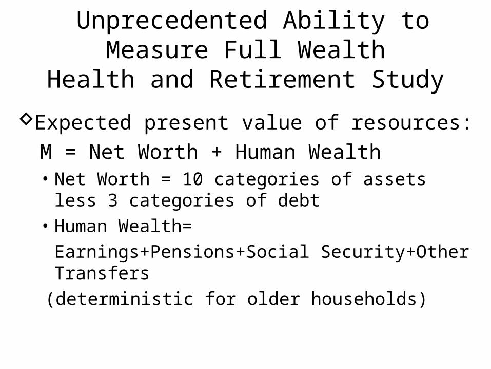
Unprecedented Ability to Measure Full WealthHealth and Retirement Study
Expected present value of resources:
M = Net Worth + Human Wealth• Net Worth = 10 categories of assets less 3 categories
of debt• Human Wealth=
Earnings+Pensions+Social Security+Other Transfers
(deterministic for older households)

Full Wealth is Not Just Scaled-Up Net Worth
Age Profile of Wealth
20
0,0
00
40
0,0
00
60
0,0
00
80
0,0
00
10
0000
0
55 60 65 70 75Age of Household Head
Full Wealth Cash-on-Hand Net Worth
Full Wealth
Net worth
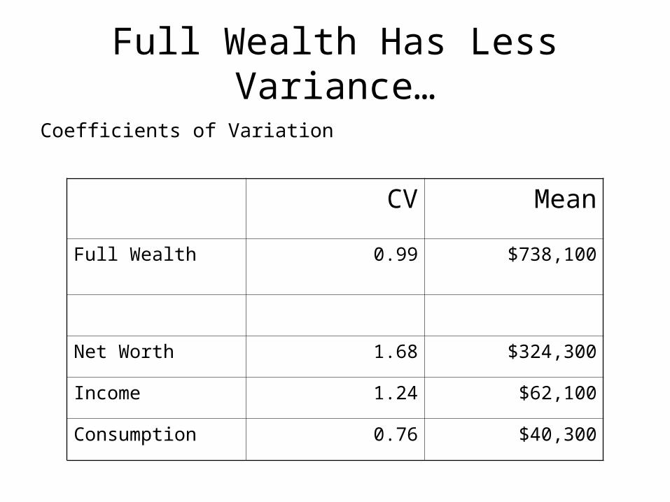
Full Wealth Has Less Variance…
Coefficients of Variation
CV Mean
Full Wealth 0.99 $738,100
Net Worth 1.68 $324,300
Income 1.24 $62,100
Consumption 0.76 $40,300

…and is more equally distributed0
.2.4
.6.8
1
0 .2 .4 .6 .8 1Cumulative population proportion
Lorenz Curve Full Wealth Lorenz Curve Net Worth
Full Wealth
Net worth
Lorenz Curves
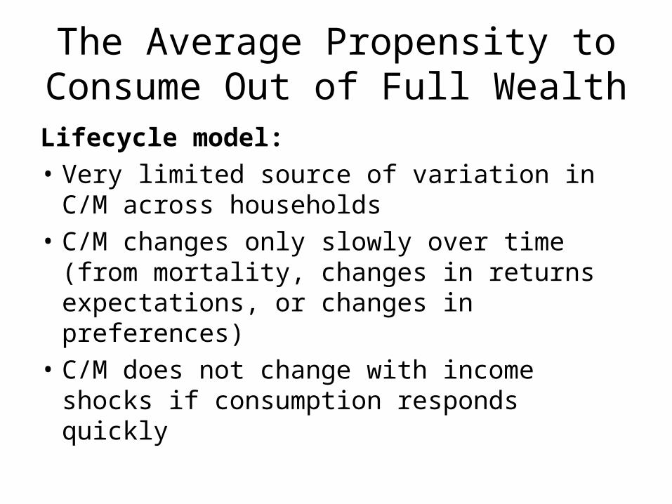
The Average Propensity to Consume Out of Full Wealth
Lifecycle model:
• Very limited source of variation in C/M across households
• C/M changes only slowly over time (from mortality, changes in returns expectations, or changes in preferences)
• C/M does not change with income shocks if consumption responds quickly

Which Implies…
Relative to C/Income or C/NetWorth, C/M Should Have:
• Lower variance• Higher covariance over time• Lower correlation with “circumstances” such as:
– Income Profile• Having a pension or the generosity of pension and social security
benefits (income replacement rate in retirement) • Earnings profile over lifetime
– Past Income Shocks
Also ∆(C/M) Should Have:• Lower correlation with past shocks both to income and
to full wealth

And the data says…
Std. Dev. Mean Median CV
C/M 2001 .058 .078 .060 0.74
C/M 2003 .062 .084 .067 0.74
C/NW 2001 3.26 1.05 .221 3.10
C/NW 2003 12.56 2.59 .256 4.85
C/I 2001 1.47 1.22 .828 1.20
C/I 2003 1.37 1.24 .888 1.10
Lower and more consistent variance

Covariance 2001&2003
C/M 0.70
C/NW 0.37
C/I 0.27
And higher covariance over time

Circumstances
• Traditional savings or consumption rates (C/I) have “noise” from circumstances, both cross-sectionally and longitudinally
• Examples:– Households expecting generous DB pension
income will save less than otherwise identical households with little or no DB pension
– Households experiencing a temporary positive income shock will save more that period

Lifecycle Model Illustrations
Standard Lifecycle Consumption
Age
Consumption Income Net Worth

Rates of Consumption Out of Alternate Measures of Resources: Income and Full Wealth
20 23 26 29 32 35 38 41 44 47 50 53 56 59 62 65 68 71 74 77 80
Age
Rat
e of
C
onsu
mpt
ion
C/Income C/Full Wealth

Comparison of Baseline to Household with Lower Retirement Income
Income and Net Worth with Different Retirement Incomes
Income Net Worth Baseline Income Baseline Net Worth
`
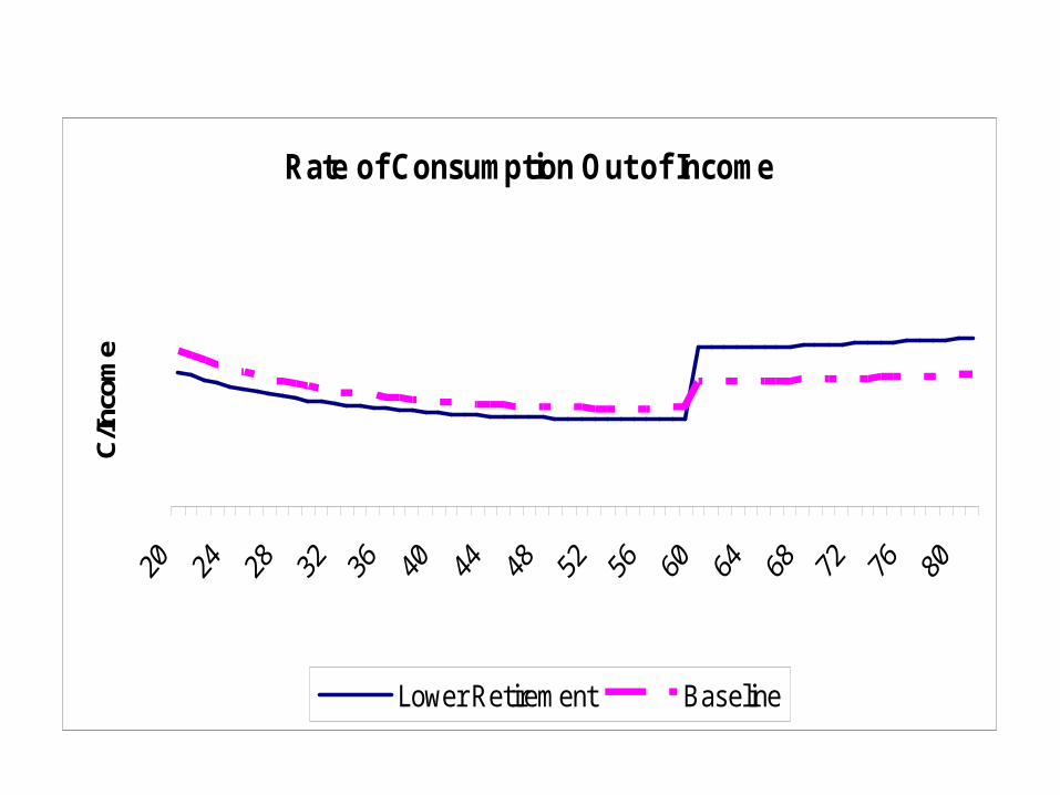
Rate of Consumption Out of Income
C/In
com
e
Lower Retirement Baseline

Consumption Rate Out of Full Wealth with Different Retirement Incomes
Age
Rat
e of
C
onsu
mpt
ion
Lower Retirement Baseline
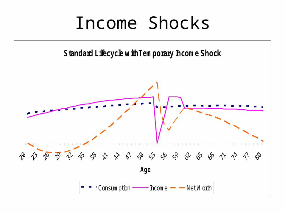
Income Shocks
Standard Lifecycle withTemporary Income Shock
Age
Consumption Income Net Worth

Comparison of Baseline and Shocked Household
Consumption Rate Out of Income with Income Shock
Age
Rat
e o
f C
on
sum
pti
on
C/I With Shock C/I Baseline
Consumption Rate Out of Full Wealth with Income Shock
AgeC/
M
C/M with Shock C/M Baseline

Testing Circumstances
Circumstance: Generosity of retirement benefits (DB pension and Social Security)
Measure:
RetRatio= Ratio of PV(Pension+Social Security) to Average Earnings Over Ages 45-55
Outcome: C/M is less correlated

Retirement/Earnings Ratio
Bivariate OLS Coefficient & T-stat R2
std(C/M) 2001 on RetRatio 0.003 (1.2) 0.00
std(C/NW) 2001 on RetRatio 0.013*** (6.0) 0.03
std(C/I) 2001 on RetRatio 0.005** (2.1) 0.01
std(C/M) 2003 on RetRatio -0.001 (-0.4) 0.00
std(C/NW) 2003 on RetRatio 0.016*** (4.8) 0.03
std(C/I) 2003 on RetRatio 0.007** (2.3) 0.01
Coefficients represent fraction of standard deviation from mean so can be compared across dependent variables

Income Shocks
Circumstance: Past Income Shock
Measure: Change in Earnings over previous years
Outcome With Levels: results mixed: C/M less correlated than C/I in 2001; less correlated for large shocks in 2003
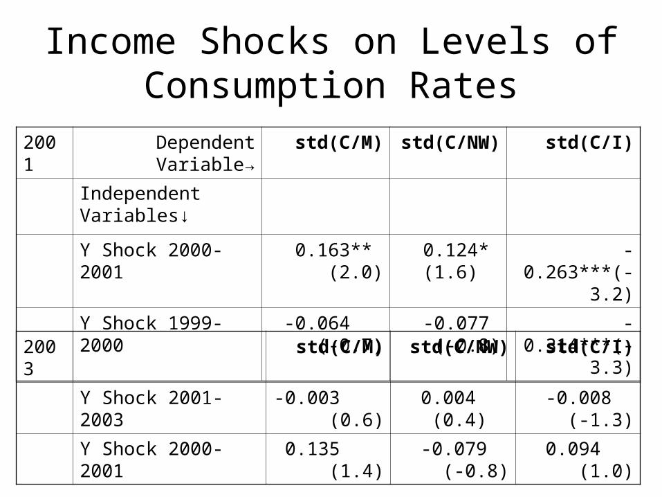
Income Shocks on Levels of Consumption Rates
2001 Dependent Variable→ std(C/M) std(C/NW) std(C/I)
Independent Variables↓
Y Shock 2000-2001 0.163** (2.0) 0.124* (1.6) -0.263***(-3.2)
Y Shock 1999-2000 -0.064 (-0.7) -0.077 (-0.8) -0.314***(-3.3)
2003 std(C/M) std(C/NW) std(C/I)
Y Shock 2001-2003 -0.003 (0.6) 0.004 (0.4) -0.008 (-1.3)
Y Shock 2000-2001 0.135 (1.4) -0.079 (-0.8) 0.094 (1.0)
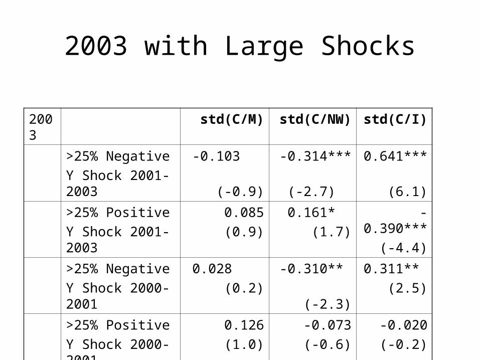
2003 with Large Shocks
2003 std(C/M) std(C/NW) std(C/I)
>25% Negative
Y Shock 2001-2003
-0.103
(-0.9)
-0.314***
(-2.7)
0.641***
(6.1)
>25% Positive
Y Shock 2001-2003
0.085
(0.9)
0.161*
(1.7)
-0.390***
(-4.4)
>25% Negative
Y Shock 2000-2001
0.028
(0.2)
-0.310**
(-2.3)
0.311**
(2.5)
>25% Positive
Y Shock 2000-2001
0.126
(1.0)
-0.073
(-0.6)
-0.020
(-0.2)
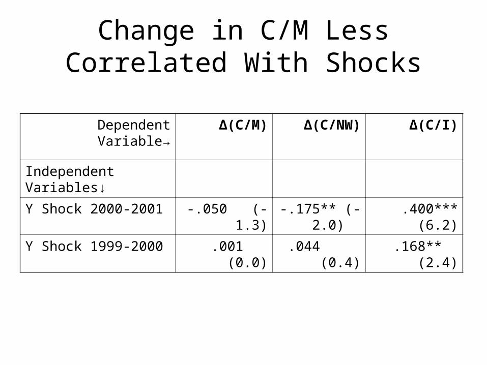
Change in C/M Less Correlated With Shocks
Dependent Variable→ ∆(C/M) ∆(C/NW) ∆(C/I)
Independent Variables↓
Y Shock 2000-2001 -.050 (-1.3) -.175** (-2.0) .400*** (6.2)
Y Shock 1999-2000 .001 (0.0) .044 (0.4) .168** (2.4)

Changes in M
• Since M is an expected value of current and future resources, any change in M must be unexpected, unlike a change in income
• If consumers adjust relatively quickly to changes in M, then C/M should be relatively invariant to such changes
• Instrument for change in M: Unexpected retirement
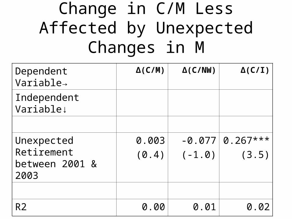
Change in C/M Less Affected by Unexpected Changes in M
Dependent Variable→ ∆(C/M) ∆(C/NW) ∆(C/I)
Independent Variable↓
Unexpected Retirement between 2001 & 2003
0.003
(0.4)
-0.077
(-1.0)
0.267***
(3.5)
R2 0.00 0.01 0.02
Conclusion
• Empirically, full wealth, M, and C/M match expected distribution characteristics
• The level of C/M has less correlation with tested circumstances than either C/NW or C/I
• The change in C/M is relatively invariant to recent income and employment shocks and changes in M when compared to C/NW or C/I