Full Title: TESTING THE ASSERTION THAT EMERGING ASIAN STOCK MARKETS ARE BECOMING MORE EFFICIENT
Authors: Kian-Ping Lima, b, Robert D. Brooksb* and Melvin J. Hinichc
Affiliations: a Labuan School of International Business and Finance Universiti Malaysia Sabah
b Department of Econometrics and Business Statistics Faculty of Business and Economics Monash University c Applied Research Laboratories
University of Texas at Austin Abstract: Testing the assertion that emerging stock markets are becoming
more efficient over time has received increasing attention in the empirical literature in recent years. However, the statistical tests adopted in extant literature are designed to detect linear predictability, and hence disregard the possible existence of nonlinear predictability. Motivated by this concern, this study computes the bicorrelation statistics of Hinich (1996) in fixed-length moving sub-sample windows, and found that nonlinear predictability for all returns series follows an evolutionary time path. However, for most indices with the exception of Taiwan SE Weighted, there is no clear trend towards higher efficiency as predicted by the classical EMH.
JEL Classification: G15; C49. Keywords: Predictability; Nonlinearity; Market Efficiency; Bicorrelations;
Emerging stock markets.
* Corresponding author.
I. INTRODUCTION
In conventional market efficiency studies using standard statistical tests, market
efficiency is measured as a property that is steady over some predefined period. In
other words, these tests lead to the inference that a market either is or is not weak-form
efficient for the sample as a whole. However, it is reasonable to expect market
efficiency to evolve over time due to factors such as institutional, regulatory and
technological changes. To accommodate this possibility, the common approach adopted
by earlier studies is to divide the sample periods into sub-periods on the basis of their
postulated factors and observe the changes in efficiency test results. For instance, in an
effort to identify the impact of regulatory changes on the efficient functioning of the
Istanbul Stock Exchange, Antoniou et al. (1997) argued in favour of examining the
evolution of the stock market, rather than simply taking a snapshot of the market at a
particular point in time. By investigating efficiency on a yearly basis over the period
1988-1993, the results show that the Istanbul Stock Exchange became efficient when
the right institutional and regulatory framework is in place. To address the question of
whether changes in the regulations governing the direct involvement of banks in the
stock market would have any significant effects on market efficiency, Groenewold et
al. (2003, 2004) examined market efficiency over three different sub-periods in which
banks were subjected to different regulations. Similarly, using sub-periods analysis,
Odabaşi et al. (2004) investigated whether the rapid development of the Istanbul Stock
Exchange in a decade of existence has rendered the market to become a relatively more
efficient market. In the wake of the movement towards financial liberalization in
emerging markets, a number of researchers have explored the issue of whether the
opening of these markets to foreign investors has caused stock markets to become more
efficient, by examining the degree of efficiency before and after the date of
2
liberalization (see, for example, Groenewold and Ariff, 1998; Kawakatsu and Morey,
1999a, b; Basu et al., 2000; Kim and Singal, 2000a, b; Maghyereh and Omet, 2002;
Laopodis, 2003, 2004).
The limitation with the above sub-periods analysis is that the movement towards
market efficiency is assumed to take the form of a discrete change that occurs at a point
in time on the basis of some postulated factors. The possibility of a continuous and
smooth change in the behaviour of stock prices over time has only been explored in
recent years using more advanced methodologies. The first group of study pioneered by
Emerson et al. (1997) applied the Kalman Filter framework that allows for time-
varying parameters and a Generalized Autoregressive Conditional Heteroscedasticity
(GARCH) structure for the residuals. In this framework, the time-varying
autoregressive coefficients were used to gauge the changing degree of predictability,
and hence evolving weak-form market efficiency. If the market under study becomes
more efficient over time, the smoothed time varying estimates of the autocorrelation
coefficient would gradually converge towards zero and become insignificant. This
framework was later formalized by Zalewska-Mitura and Hall (1999) as Test for
Evolving Efficiency (TEE) to provide an indicator of the degree of market inefficiency
and the timing and speed of the movement towards efficiency. Given that the emerging
markets in Bulgaria and Hungary were still in the early stages of development,
Emerson et al. (1997) and Zalewska-Mitura and Hall (1999) argued that it is not
sensible to address the issue of whether the stock markets in these transition economies
are efficient or not. The main reason is that when a market first opens, it is hardly
credible for the market to be efficient since it takes time for the price discovery process
to become known. However, as markets operate and market microstructures develop,
3
within a finite amount of time, they are likely to become more efficient. Hence, the
more relevant research question is whether and how these infant markets are becoming
more efficient, and this certainly cannot be answered by classical steady-variable
approaches that assume a fixed level of market efficiency throughout the entire
estimation period. In fact, the early inefficiency would bias the results of these
conventional tests and lead to the conclusion that there are profit opportunities simply
because of past inefficiencies (see Emerson et al., 1997; Zalewska-Mitura and Hall,
1999). Using the proposed TEE, their results revealed varying degrees of inefficiency
in those markets under study and the respective time paths towards efficiency. This
framework was subsequently adopted to assess the evolution of efficiency in other
stock markets in Central and Eastern European transition economies that have just
emerged out of the former communist bloc (see, for example, Zalewska-Mitura and
Hall, 2000; Rockinger and Urga, 2000, 2001). Hence, it is not surprising that the TEE
literature has been expanding to test a wider set of markets including the Chinese (Li,
2003a, b) and African stock markets (Jefferis and Smith, 2004, 2005). Along the same
line, Kvedaras and Basdevant (2004) proposed the time-varying variance ratio statistic
that is based on time-varying autocorrelation coefficients estimated using the Kalman
filter technique, and applied the methodology to track the changing degree of market
efficiency in Estonia, Latvia and Lithuania.
Another strand of study employs fixed-length moving sub-sample windows approach to
test the evolution of market efficiency in emerging stock markets. This rolling windows
approach computes the relevant test statistic that is capable of detecting serial
dependence for the first window of a specified length, and then rolls the sample one
point forward eliminating the first observation and including the next one for re-
4
estimation of the test statistic. This process continues until the last observation is used.
For instance, in a fixed-length rolling windows of 30 observations, the first window
starts from day 1 and ends on day 30, the second window comprises observations
running from day 2 through day 31, and so on. The last window is built with the last 30
observations. To accommodate the dynamics of the stock price process, Tabak (2003)
examined the random walk hypothesis using rolling variance ratio tests with a fixed
window of 1024 days, and concluded that the Brazilian stock market has become
increasingly more efficient.1 Besides the popular variance ratio test, the Hurst exponent
has been explored by Costa and Vasconcelos (2003) to assess the efficiency of
Brazilian stock market using 30 years of daily data from 1968 to 2001. The authors
argued that a Hurst exponent (H) of 0.5 for the whole sample period does not
necessarily imply the absence of long-range correlations, since this could be due to the
averaging of those positive and negative correlations at different time periods.2 Indeed,
the results from the rolling 3-year time windows approach support their conjecture that
the Hurst exponent varies considerably over time.3 In particular, the exponent is always
greater than 0.5 before 1990 with the only exception occurring around the year 1986,
and drops rapidly towards 0.5 in early 1990. After that, H stays around 0.5 with minor
1 Yilmaz (2003) has also adopted the rolling variance ratio test to observe whether there is any change in
the behaviour of exchange rates over time.
2 Briefly, there is no evidence of temporal dependence between observations widely separated in time if
H = 0.5, indicating that the series under examination behaves in a manner consistent with weak-form
efficient market hypothesis (EMH). On the other hand, H > 0.5 indicates that linear associations between
distant observations is somewhat persistent, while there is evidence of long-term dependence with anti-
persistent behaviour if H < 0.5.
3 In the foreign exchange market, evidence of time-varying Hurst exponents was documented in
Vandewalle and Ausloos (1997) and Muniandy et al. (2001).
5

fluctuations, suggesting that the market has become more efficient during this period.
Cajueiro and Tabak (2004a) formally proposed the calculation of Hurst exponent over
time for stock returns using the rolling sample approach as a statistical tool to test the
assertion that emerging stock markets are becoming more efficient. The authors argued
that stock markets have presented different levels of efficiency over time mainly due to
the variation of the effects of (a) speed of information, (b) capital flows, and (c) non-
synchronous trading. Using a 4-year time windows, and stock data from eleven
emerging markets, plus the U.S. and Japan for comparison, the Hurst exponent is found
to be time-varying reflecting the evolution of market efficiency over time in each
market under study. The changing degree of long-term predictability is also reported
for stock markets in European transition economies by Cajueiro and Tabak (2006).
Using similar approach, Cajueiro and Tabak (2004b, c) computed the Hurst exponent
over time and build a ranking based on the medians of those computed Hurst exponent
to assess the relative efficiency of stock markets. An alternative framework for testing
evolving market efficiency was later proposed by Cajueiro and Tabak (2005a, b), in
which the Hurst exponent was computed for the volatility of stock returns, measured by
absolute and squared returns.
The above discussion clearly demonstrates that it is not sensible for conventional
efficiency studies to assume markets are in some kind of steady-state, especially for
emerging stock markets. In this regard, those cited statistical tests offer useful
framework to capture the evolving dynamics of the detected patterns over time. The test
for evolving efficiency (Zalewska-Mitura and Hall, 1999), rolling variance ratio test
(Tabak, 2003), time-varying variance ratio test (Kvedaras and Basdevant, 2004) are
designed to capture the changing degree of autocorrelation coefficients of lower lag
6
orders over time. On the other hand, the framework of time-varying Hurst exponents
(Costa and Vasconcelos, 2003) detects the presence of long-term dependence, in which
the autocorrelation function decays at a hyperbolic rate and remains significant even at
long lags. As far as financial markets are concerned, the existence of both types of
linear dependence, be it short-term or long-term, provides evidence against the weak-
form efficient market hypothesis (EMH) which implies unpredictability of future
returns based on historical returns. This study focuses on another type of temporal
dependence that appears inconsistent with the unpredictable criterion of market
efficiency, and has been neglected in this line of empirical inquiry. In particular, given
that predictability is assumed to take the form of linear correlations in those cited
literature, the main objective of this paper is to demonstrate that detecting nonlinear
dependence in a moving time windows provides further insight into the changing
degree of market efficiency over time.
There are a number of reasons why nonlinear dependence should not be discarded in
the empirical investigation of whether emerging stock markets are becoming more
efficient. First, partly due to the development of new statistical tools capable of
uncovering any hidden nonlinear structures in time series data4, overwhelming
evidence in support of nonlinear serial dependence has been documented across
international stock markets with different market structure mechanisms, indicating that
the observed feature is a stylized fact of real financial data. This growing body of
research includes the U.S. (Hinich and Patterson, 1985; Ashley and Patterson, 1989;
4 For a review of those existing non-linearity tests that are widely employed in the literature, see Granger
and Teräsvirta (1993), Barnett et al. (1997), Patterson and Ashley (2000) and Kyrtsou and Serletis
(2006).
7

Scheinkman and LeBaron, 1989; Brock et al., 1991; Hsieh, 1991; Kohers et al., 1997;
Patterson and Ashley, 2000; Urrutia et al., 2002), U.K. (Abhyankar et al., 1995; Al-
Loughani and Chappell, 1997; Omran, 1997; Chappel et al., 1998; Opong et al., 1999;
Yadav et al., 1999; McMillan, 2003), and other national stock markets (De Gooijer,
1989; Sewell et al., 1993; Hsieh, 1995; Abhyankar et al., 1997; Pandey et al., 1998;
Freund and Pagano, 2000; Sarantis, 2001; Ammermann and Patterson, 2003; Appiah-
Kusi and Menyah, 2003; Shively, 2003; Lim and Liew, 2004; Narayan, 2005). Second,
the existence of nonlinear dependence implies the potential of predictability, thus
posing a serious threat to the weak-form EMH. Brooks and Hinich (1999) argued that if
the nonlinearity is present in the conditional first moment, it may be possible to devise
a trading strategy based on nonlinear models which is able to yield higher returns than a
buy-and-hold rule. Neftci (1991) demonstrated that in order for technical trading rules
to be successful, some form of nonlinearity in stock prices is necessary. In testing the
primary hypothesis that graphical technical analysis methods may be equivalent to non-
linear forecasting methods, Clyde and Osler (1997) found that technical analysis works
better on nonlinear data than on random data, and the use of technical analysis can
generate higher profits than a random trading strategy if the data generating process is
non-linear. The potential of nonlinear predictability generated considerable excitement
in the financial econometrics community that led to an explosive growth of nonlinear
time series models over the years (see, for example, Tong, 1990; Granger and
Teräsvirta, 1993; Franses and van Dijk, 2000). Third, widely applied efficiency tests,
such as autocorrelation, variance ratio and spectral tests are not capable of capturing
nonlinearity, and may deliver misleading conclusion especially in cases where the
underlying series have zero autocorrelation yet possess predictable nonlinearities in
mean, such as those generated by bilinear and nonlinear moving average processes.
8

Motivated by this concern, a number of studies re-examined the weak-form market
efficiency using statistical tests that are capable of detecting nonlinear serial
dependence (see, for example, Al-Loughani and Chappell, 1997; Antoniou et al., 1997;
Kohers et al., 1997; Chappel et al., 1998; Opong et al., 1999; Freund and Pagano, 2000;
Appiah-Kusi and Menyah, 2003; Narayan, 2005).
To capture the evolving property of nonlinear predictable patterns, this study adopts the
research framework proposed by Hinich and Patterson (1995). In particular, this
approach first divides the full sample period into equal-length non-overlapped moving
time windows, and then computes the Hinich (1996) portmanteau bicorrelation test
statistic that is designed to detect nonlinear serial dependence in each window. This
nonlinearity test is the preferred choice for two reasons. First, it has good sample
properties over short horizons of data (Hinich and Patterson, 1995, Hinich, 1996).
Second, the test suggests an appropriate functional form for a nonlinear forecasting
equation. In particular, Brooks and Hinich (2001) demonstrated via their proposed
univariate bicorrelation forecasting model that the bicorrelations can be used to forecast
the future values of the series under consideration. In the present framework, the
evolution of nonlinear predictable patterns can be captured by the moving time
windows. Specifically, by plotting the bicorrelation test statistic as a function of time, it
permits a closer examination of the precise time periods during which nonlinear serial
dependence are occurring. In the literature, this approach has been applied on financial
time series data (see, for example, Brooks and Hinich, 1998; Brooks et al., 2000;
Ammermann and Patterson, 2003; Lim and Hinich, 2005a, b; Bonilla et al., 2006).
9

The plan of this paper is as follows. Section II discusses the research framework
adopted in this study. Following that, description of the data and discussion on the
empirical results are provided. The final section concludes the paper.
II. PORTMANTEAU CORRELATION AND BICORRELATION TEST
STATISTICS IN MOVING TIME WINDOWS
The research framework adopted in this study was first proposed by Hinich and
Patterson (1995), now published as Hinich and Patterson (2005). It involves a
procedure of dividing the full sample period into equal-length non-overlapped moving
time windows, in which the window length is an arbitrary choice. Suppose that a 30-
day window length is chosen, the first window comprises the first 30 sample data
points, starts from day 1 and ends on day 30. The second window comprises
observations running from day 31 through day 60. Subsequent windows will follow in a
similar manner until the end of the data series is reached. However, the last window is
not used if there are not 30 observations to fill that window. In principle, this approach
is similar to the rolling time windows given that the window length in both approaches
is fixed. The only difference lies on how the time windows move forward. The data in
each window is standardized to have a sample mean of zero and a sample variance of
one by subtracting the sample mean of the window and dividing by its standard
deviation in each case. Subsequently, two test statistics are calculated for the
standardized data in each window. The first one is a portmanteau correlation test
statistic, denoted as the C statistic, which is a modified version of the Box-Pierce Q-
statistic. Unlike the Box-Pierce Q-statistic that was usually applied to the residuals of a
fitted ARMA model, the C statistic is a function of the standardized observations and
10
the number of lags used depends on the sample size. The second test statistic is the
portmanteau bicorrelation test statistic denoted as the H statistic, which is a third-order
extension of the standard correlation test for white noise. The null hypothesis for each
window is that the standardized data are realizations of a stationary pure white noise
process that has zero correlation and bicorrelation. Under the null hypothesis, the
distribution of the C and H statistics are asymptotically chi-squared with degrees of
freedom equal to L and (L-1)(L/2) respectively, where L is the number of lags that
define the window.5 Using the two portmanteau test statistics, the proposed research
framework looks for those windows in which the time series exhibits behaviour that
departs significantly from pure white noise in terms of linear serial dependence
(significant autocorrelations detected by C statistic) or nonlinear serial dependence
(significant bicorrelations detected by H statistic). In other words, the null hypothesis is
rejected if the process in the window has some non-zero correlations or bicorrelations,
implying the potential of predictability for the series under consideration. The full
theoretical derivation of the test statistics and some Monte Carlo evidence on the small
sample properties of both test statistics are given in Hinich (1996) and Hinich and
Patterson (1995, 2005).
Mathematical Representation
Let the sequence {y(t)} denote the sampled data process, where the time unit, t, is an
integer. The test procedure employs non-overlapped time windows, thus if n is the
window length, then the k-th window is {y(tk), y(tk+1),…, y(tk+n-1)}. The next non-
overlapped window is {y(tk+1), y(tk+1+1),….. y(tk+1+n-1)}, where tk+1 = tk+n. The null 5 The proofs for the asymptotic property of C and H statistics are given in Box and Pierce (1970) and
Hinich (1996) respectively.
11

hypothesis for each time window is that y(t) are realizations of a stationary pure white
noise process. Thus, under the null hypothesis, the correlations Cyy(r) = E[y(t)y(t+r)]
and bicorrelations Cyyy(r, s) = E[y(t)y(t+r)y(t+s)] are all equal to zero for all r, s except
when r = s = 0. The alternative hypothesis is that the process in the window has some
non-zero correlations or bicorrelations in the set 0 < r < s < L, where L is the number of
lags that define the window. In other words, if there exists second-order linear or third-
order nonlinear dependence in the data generating process, then Cyy(r) ≠ 0 or Cyyy(r, s) ≠
0 for at least one r value or one pair of r and s values respectively.
Define Z(t) as the standardized observations obtained as follows:
( )( ) y
y
y t mZ t
s−
= (1)
for each t = 1, 2,………, n where my and sy are the sample mean and sample standard
deviation of the window.
The r sample correlation coefficient is:
12
1( ) ( ) ( ) ( )
n r
ZZt
C r n r Z t Z t r−−
=
= − +∑ (2)
The C statistic, which is developed to test for the existence of non-zero correlations (i.e.
linear dependence) within a window, and its corresponding distribution are:
12
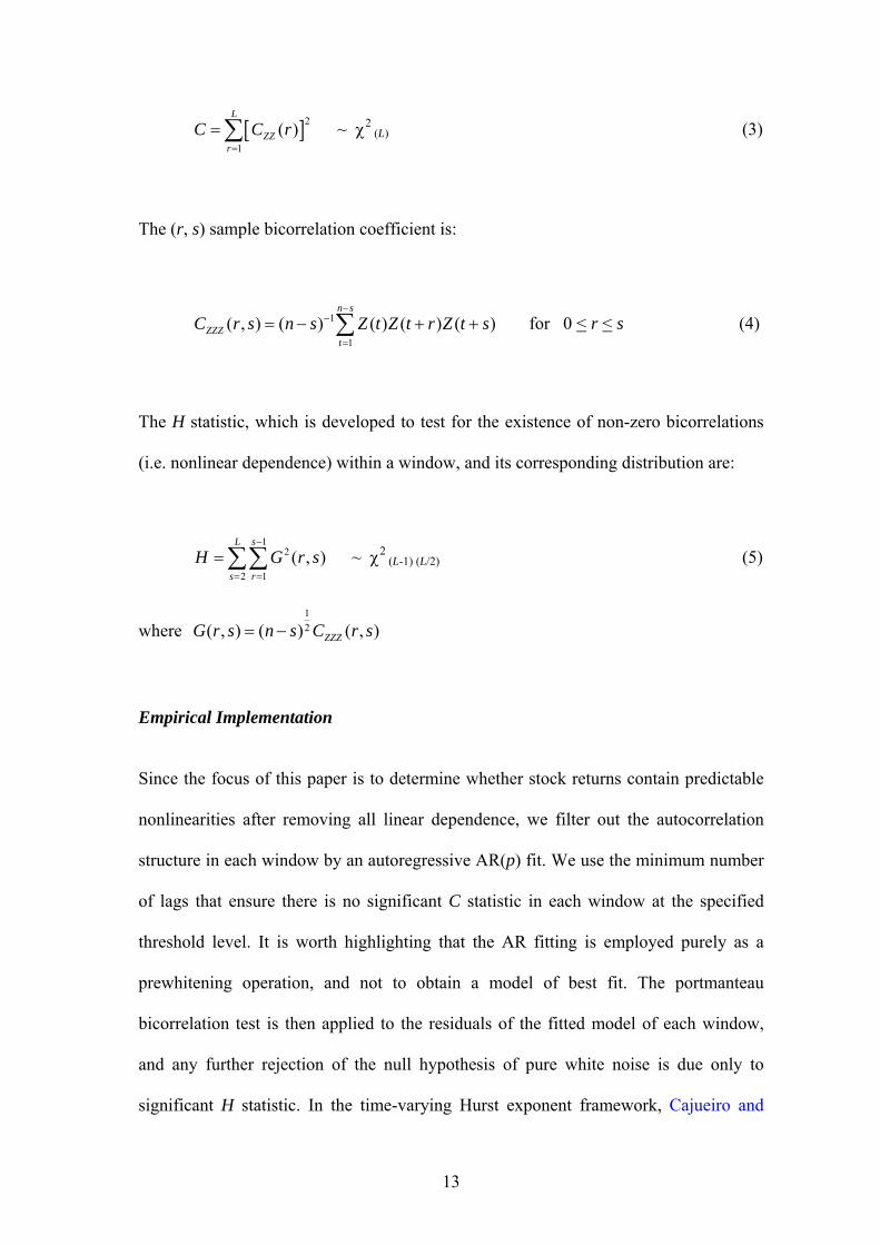
[ 2
1( )
L
ZZr
C C r=
= ∑ ] ~ χ2 (L) (3)
The (r, s) sample bicorrelation coefficient is:
1
1( , ) ( ) ( ) ( ) ( )
n s
ZZZt
C r s n s Z t Z t r Z t s−
−
=
= − +∑ + for 0 < r < s (4)
The H statistic, which is developed to test for the existence of non-zero bicorrelations
(i.e. nonlinear dependence) within a window, and its corresponding distribution are:
12
2 1( , )
L s
s rH G r s
−
= =
= ∑∑ ~ χ2 (L-1) (L/2) (5)
where 12( , ) ( ) ( , )ZZZG r s n s C r s= −
Empirical Implementation
Since the focus of this paper is to determine whether stock returns contain predictable
nonlinearities after removing all linear dependence, we filter out the autocorrelation
structure in each window by an autoregressive AR(p) fit. We use the minimum number
of lags that ensure there is no significant C statistic in each window at the specified
threshold level. It is worth highlighting that the AR fitting is employed purely as a
prewhitening operation, and not to obtain a model of best fit. The portmanteau
bicorrelation test is then applied to the residuals of the fitted model of each window,
and any further rejection of the null hypothesis of pure white noise is due only to
significant H statistic. In the time-varying Hurst exponent framework, Cajueiro and
13
Tabak (2004a) filtered the data in each window by means of an AR-GARCH procedure
to account for short-term autocorrelation and time-varying volatility commonly found
in financial returns series. However, Brooks and Hinich (2001) argued that this
procedure is unnecessary with the bicorrelation test since the presence of GARCH
effects will not cause a rejection of the null hypothesis of pure white noise. This is due
to the fact that the GARCH process has zero bicorrelation, and hence, the bicorrelation
test will have the proper size, asymptotically, even in the presence of GARCH effects
(see also Ammermann and Patterson, 2003).6
The number of lags L is specified as L = nb with 0 < b < 0.5, where b is a parameter
under the choice of the user. All lags up to and including L are used to compute the
bicorrelations in each window. Based on the results of Monte Carlo simulations,
Hinich and Patterson (1995, 2005) recommended the use of b=0.4 in order to maximize
the power of the tests while ensuring a valid approximation of the asymptotic theory
even when n is small. Another element that must be decided upon is the choice of the
window length. In fact, there is no unique value for the window length. The larger the
window length, the larger the number of lags and hence the greater the power of the
test, but it increases the uncertainty on the event time when the serial dependence
occurs. In this study, the data are split into a set of equal-length non-overlapped moving
time windows of 50 observations. This window length is sufficiently long enough to
6 Nonetheless, Hinich and Patterson (1995, 2005) demonstrated that the presence of ARCH/GARCH
effects does not cause false rejection by the H statistic in two different ways. First, a computer simulation
of a GARCH model is carried out, and the size of the H statistic is reported. Second, the simulated
GARCH data is transformed to a binary series (0, 1), turning the GARCH into a pure white noise
process, and then evaluate the size of the H statistic. In both instances, the H statistic has the appropriate
size. See also Brooks and Hinich (1998) and Brooks et al. (2000).
14
validly apply the test and yet short enough for the data generating process to have
remained roughly constant.
The H statistic for each window in this study is computed using the T23 FORTRAN
program.7 Instead of reporting the test statistics as chi-square variates, the program
transforms the computed statistics to p-values based on the appropriate chi square
cumulative distribution value, since it is a simple and informative way of summarizing
the results of statistical test. If the p-value for the H statistic in a particular window is
sufficiently low, then one can reject the null hypothesis of pure white noise that has
zero bicorrelation. In this case, the significant H statistic indicates the presence of
nonlinear dependence in that window. In the present study, a window is defined as
significant if the H statistic rejects the null hypothesis at the specified threshold level
for the p-value, which is set at 5% in the empirical analysis. To offer further
improvement to the size of the test in small samples, resampling with replacement
(Efron, 1979) that satisfy the null hypothesis is used to determine a threshold for the H
statistic that has a test size to be 5%. Hence, the null hypothesis in each window is
rejected when the p-value for the H statistic is less than or equal to the bootstrapped
threshold drawn from 5000 replications that corresponds to the specified nominal
threshold level of 5%.
7 The T23 FORTRAN program can be downloaded from http://www.gov.utexas.edu/hinich/.
15

III. EMPIRICAL APPLICATIONS
The Data
The present study utilizes indices at daily frequency for ten emerging stock markets in
Asia as categorized by Standard & Poor’s Global Stock Markets Factbook 2004: China
(Shanghai SE Composite), India (India BSE National), Indonesia (Jakarta SE
Composite), South Korea (Korea SE Composite), Malaysia (Kuala Lumpur
Composite), Pakistan (Karachi SE 100), Philippines (Philippines SE Composite), Sri
Lanka (Colombo SE All Share), Taiwan (Taiwan SE Weighted) and Thailand
(Bangkok S.E.T.). All the closing prices of these indices collected from Datastream are
denominated in their respective local currency units for the sample period 1/1/1992 to
31/12/2005. The data are transformed into a series of continuously compounded
percentage returns by taking 100 times the log price relatives, i.e. rt = 100* ln(pt/pt-1),
where pt is the closing price of the index on day t, and pt-1 the price on the previous
trading day. This transformation yields 3130 observations for the empirical analysis.
Preliminary Analysis
Table 1 provides the summary statistics for the returns series of all the ten Asian stock
indices. Notably, the China stock market exhibits the highest level of volatility. Most of
the indices exhibit some degree of right-skewness, with the exception of Pakistan,
South Korea and Taiwan. On the other hand, the distributions are highly leptokurtic, in
which the tails of their respective distributions taper down to zero more gradually than
do the tails of a normal distribution. Not surprisingly, given the non-zero skewness
16

levels and excess kurtosis, the Jarque-Bera (JB) test statistics clearly indicate that all
returns series under study significantly deviate from normality.
The lower panel of Table 1 reports the autocorrelation coefficients for the first five
lags. In all cases except Taiwan, the first order autocorrelation coefficient is statistically
significant, and its magnitude is generally higher than those of longer lags. Even so,
there is still evidence of significant autocorrelation at lags higher than one. Moreover,
the null hypothesis of autocorrelation for all orders up to lag 10 is strongly rejected by
the Ljung-Box Q-statistic. Taken as a whole, these results clearly indicate the presence
of linear dependence in the daily returns series of all indices.
<<Insert Table 1 about here>>
Evidence of Nonlinearity
To test whether nonlinear serial dependence also plays an important role in the data
generating process, in addition to the autocorrelations identified earlier, this study
employs a battery of univariate nonlinearity tests outlined in Patterson and Ashley
(2000). These tests are selected for two reasons. First, most of the existing tests have
differing power against different classes of nonlinear processes and none dominates all
others (see, for example, Ashley et al., 1986; Ashley and Patterson, 1989; Hsieh, 1991;
17
Lee et al., 1993; Brock et al., 1991, 1996; Barnett et al., 1997; Patterson and Ashley,
2000). Second, the estimations can be carried out using the Nonlinear Toolkit provided
by Patterson and Ashley (2000), and it been used in the literature by Panagiotidis
(2002, 2005), Panagiotidis and Pelloni (2003) and Ashley and Patterson (2006).8 It is
important to note that the main objective is not to determine the precise nature of the
nonlinearity but to determine whether or not nonlinearity exists in the full sample of the
returns series under study.
The battery of nonlinearity tests included in the toolkit are: McLeod-Li test (McLeod
and Li, 1983), Engle LM test (Engle, 1982), BDS test (Brock et al., 1996), Tsay test
(Tsay, 1986), bicorrelation test (Hinich, 1996) and bispectrum test (Hinich, 1982).9
With the exception of the bispectrum test, each of these tests is actually testing for
serial dependence of any kind, whether linear or nonlinear. Hence, data pre-whitening
is necessary prior to the application of these five tests in order to remove any linear
structure from the data, so that any remaining serial dependence must be due to a
nonlinear data generating mechanism. In contrast, the bispectrum test provides a direct
test for a non-linearity, irrespective of any linear serial dependence that might be
present. Ashley et al. (1986) presented an equivalence theorem to prove that the Hinich
bispectrum test is invariant to linear filtering of the data, even if the filter is estimated.
8 The toolkit can be downloaded from Richard Ashley’s webpage at
http://ashleymac.econ.vt.edu/ashleyhome.html, while instructions and interpretations of all the tests are
given in chapter 3 of Patterson and Ashley (2000).
9 The descriptions of these tests are deliberately omitted due to space constraint. The reader is to refer to
the detailed discussion in Patterson and Ashley (2000).
18

In this case, the test is robust even if linear pre-whitening model has failed to remove
all linear serial dependence in the data.10
Given the differing power of these nonlinearity tests against different classes of
nonlinear processes, it is not surprising to observe from Table 2 that ‘unanimous’
verdict on the existence of nonlinearity is reached only for six markets. In the case of
China, the Mc-Leod-Li test cannot reject the null of linearity even at the 10% level of
significance. On the other hand, the bispectrum test cannot reject the null for South
Korea, Sri Lanka and Thailand. Taken as a whole, the results indicate that nonlinearity
plays a significant role in the returns dynamics for each of the indices. Hence, the
present findings provide further support to the main argument of this paper that
empirical study on market efficiency should not implicitly disregard the possible
existence of this particular type of higher-order temporal dependence.
<<Insert Table 2 about here>>
10 Given that the size of the bispectrum test is found to be conservative for finite samples, this study
utilizes the shuffle bootstrap approach (resampling without replacement) outlined by Hinich et al. (2005)
with 1000 replications. The FORTRAN program is available from http://www.gov.utexas.edu/hinich/.
19
Results from Moving Time Windows Approach
This section proceeds to compute the bicorrelation or H statistic for each window to
determine whether those detected nonlinear serial dependence is localized in time. As
noted by Ammermann and Patterson (2003), it is possible that the significant results of
nonlinearity in the full sample are driven by the activity within a small number of sub-
periods. To conserve space and for comparison purpose, Figure 1 and 2 plot the p-
values of the H statistic in moving time windows for two selected markets- Taiwan and
Sri Lanka.11 The vertical axis shows the p-values, while across the horizontal axis are
the starting dates for each time window. In the present framework, a window is defined
as significant if the H statistic rejects the null hypothesis of pure white noise at the
specified threshold level, i.e. when the p-value of the H statistic is less than or equal to
the bootstrapped threshold that corresponds to the nominal threshold level of 5%.
Graphically, a window is significant if the p-value lies below or on the threshold line.
For instance, in the case of Taiwan (Taiwan SE Weighted)) as depicted in Figure 1,
there are six windows with strong non-zero bicorrelations and hence move the H
statistic to cross the bootstrapped threshold for the p-value of 0.0677 (dashed line), thus
implying the potential of nonlinear predictability during these particular time periods.
Table 3 provides the time periods of those windows with significant H statistic, making
it possible for future research to explore in detail the factors that generate this
predictability. It is interesting to note that after removing all short-term linear
dependence, the stock returns under study still contain predictable nonlinearities that
contradict the unpredictable criterion of weak-form EMH.
11 Figures for other stock markets are available upon request from the authors.
20
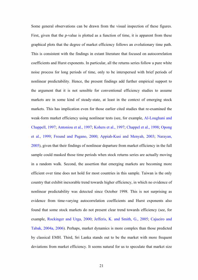
Some general observations can be drawn from the visual inspection of these figures.
First, given that the p-value is plotted as a function of time, it is apparent from these
graphical plots that the degree of market efficiency follows an evolutionary time path.
This is consistent with the findings in extant literature that focused on autocorrelation
coefficients and Hurst exponents. In particular, all the returns series follow a pure white
noise process for long periods of time, only to be interspersed with brief periods of
nonlinear predictability. Hence, the present findings add further empirical support to
the argument that it is not sensible for conventional efficiency studies to assume
markets are in some kind of steady-state, at least in the context of emerging stock
markets. This has implication even for those earlier cited studies that re-examined the
weak-form market efficiency using nonlinear tests (see, for example, Al-Loughani and
Chappell, 1997; Antoniou et al., 1997; Kohers et al., 1997; Chappel et al., 1998; Opong
et al., 1999; Freund and Pagano, 2000; Appiah-Kusi and Menyah, 2003; Narayan,
2005), given that their findings of nonlinear departure from market efficiency in the full
sample could masked those time periods when stock returns series are actually moving
in a random walk. Second, the assertion that emerging markets are becoming more
efficient over time does not hold for most countries in this sample. Taiwan is the only
country that exhibit inexorable trend towards higher efficiency, in which no evidence of
nonlinear predictability was detected since October 1998. This is not surprising as
evidence from time-varying autocorrelation coefficients and Hurst exponents also
found that some stock markets do not present clear trend towards efficiency (see, for
example, Rockinger and Urga, 2000; Jefferis, K. and Smith, G., 2005; Cajueiro and
Tabak, 2004a, 2006). Perhaps, market dynamics is more complex than those predicted
by classical EMH. Third, Sri Lanka stands out to be the market with more frequent
deviations from market efficiency. It seems natural for us to speculate that market size
21
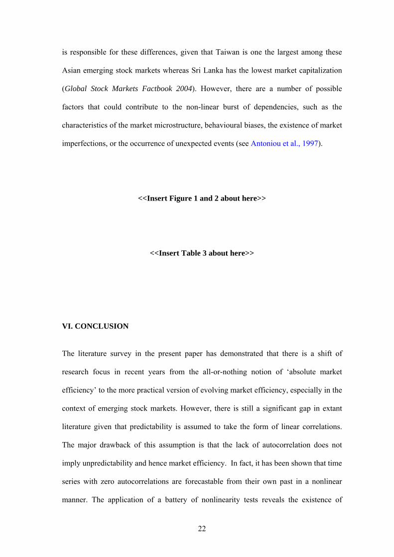
is responsible for these differences, given that Taiwan is one the largest among these
Asian emerging stock markets whereas Sri Lanka has the lowest market capitalization
(Global Stock Markets Factbook 2004). However, there are a number of possible
factors that could contribute to the non-linear burst of dependencies, such as the
characteristics of the market microstructure, behavioural biases, the existence of market
imperfections, or the occurrence of unexpected events (see Antoniou et al., 1997).
<<Insert Figure 1 and 2 about here>>
<<Insert Table 3 about here>>
VI. CONCLUSION
The literature survey in the present paper has demonstrated that there is a shift of
research focus in recent years from the all-or-nothing notion of ‘absolute market
efficiency’ to the more practical version of evolving market efficiency, especially in the
context of emerging stock markets. However, there is still a significant gap in extant
literature given that predictability is assumed to take the form of linear correlations.
The major drawback of this assumption is that the lack of autocorrelation does not
imply unpredictability and hence market efficiency. In fact, it has been shown that time
series with zero autocorrelations are forecastable from their own past in a nonlinear
manner. The application of a battery of nonlinearity tests reveals the existence of
22

nonlinear predictability in all the returns series under study, and hence contradicts the
unpredictable criterion of weak-form EMH.
Motivated by the concern that the findings of nonlinear departure from market
efficiency in the full sample could actually masked those time periods when stock
returns series are in fact pure white noise, bicorrelation or H statistics of Hinich (1996)
were estimated using fixed-length moving sub-sample windows approach. The results
reveal that the detected nonlinear predictability for all returns series is localized in time
and follows an evolutionary time path. This adds further support to the argument that
market efficiency is not an all-or-none condition but is a characteristic that varies
continuously over time. However, for most indices with the exception of Taiwan SE
Weighted, there is no clear trend towards higher efficiency as predicted by the classical
EMH. All this points to the search for an alternative hypothesis, and the statistical
features of our data are very much in line with those postulated by the Adaptive
Markets Hypothesis (AMH) of Lo (2004, 2005). According to Lo (2005), the notion
that evolving systems must march inexorably towards some ideal stationary state is
incorrect. Instead, the AMH implies considerably more complex market dynamics, with
cycles as well as trends, panics, manias, bubbles, crashes, and other phenomena that are
routinely witnessed in natural market ecologies. Based on the evolutionary perspective,
profit opportunities do exist from time to time. Though they disappear after being
exploited by investors, new opportunities are continually being created as groups of
market participants, institutions and business conditions change. Hence, the present
paper provides some interesting insight into this new paradigm that is still in its infant
stage of development.
23

ACKNOWLEDGEMENT
The authors would like to thank Richard Ashley for comments on the implementation
of the tests included in the Nonlinear Toolkit. The first author thanks Universiti
Malaysia Sabah for his PhD scholarship.
REFERENCES
Abhyankar, A., L.S. Copeland and W. Wong, 1995, Nonlinear dynamics in real-time
equity market indices: evidence from the United Kingdom, Economic Journal
105, 864-880.
Abhyankar, A., L.S. Copeland and W. Wong, 1997, Uncovering nonlinear structure in
real-time stock-market indexes: the S&P 500, the DAX, the Nikkei 225, and the
FTSE-100, Journal of Business and Economic Statistics 15, 1-14.
Al-Loughani, N. and D. Chappell, 1997, On the validity of the weak-form efficient
markets hypothesis applied to the London stock exchange, Applied Financial
Economics 7, 173-176.
Ammermann, P.A. and D.M. Patterson, 2003, The cross-sectional and cross-temporal
universality of nonlinear serial dependencies: evidence from world stock indices
and the Taiwan Stock Exchange, Pacific-Basin Finance Journal 11, 175-195.
Antoniou, A., N. Ergul and P. Holmes, 1997, Market efficiency, thin trading and non-
linear behaviour: evidence from an emerging market, European Financial
Management 3, 175-190.
Appiah-Kusi, J. and K. Menyah, 2003, Return predictability in African stock markets,
Review of Financial Economics 12, 247-270.
24
Ashley, R.A. and D.M. Patterson, 1989, Linear versus nonlinear macroeconomies: a
statistical test, International Economic Review 30, 685-704.
Ashley, R.A. and D.M. Patterson, 2006, Evaluating the effectiveness of state-switching
time series models for U.S. real output, Journal of Business and Economic
Statistics, forthcoming.
Ashley, R.A., D.M. Patterson and M.J. Hinich, 1986, A diagnostic test for nonlinear
serial dependence in time series fitting errors, Journal of Time Series Analysis
7(3), 165-178.
Barnett, W.A., A.R. Gallant, M.J. Hinich, J. Jungeilges, D. Kaplan and M.J. Jensen,
1997, A single-blind controlled competition among tests for nonlinearity and
chaos, Journal of Econometrics 82, 157-192.
Basu, P., H. Kawakatsu and M.R. Morey, 2000, Liberalization and stock prices in
emerging markets, Emerging Markets Quarterly 4(3), 7-17.
Bonilla, C.A., R. Romero-Meza and M.J. Hinich, 2006, Episodic nonlinearity in Latin
American stock market indices, Applied Economics Letters 13, 195-199.
Box, G.E.P. and D.A. Pierce, 1970, Distributions of residual autocorrelations in
autoregressive-integrated moving average time series models, Journal of the
American Statistical Association 65(332), 1509-1526.
Brock, W.A., W.D. Dechert, J.A. Scheinkman and B. LeBaron, 1996, A test for
independence based on the correlation dimension, Econometric Reviews 15, 197-
235.
Brock, W.A., D.A. Hsieh and B. LeBaron, 1991, Nonlinear dynamics, chaos, and
instability: statistical theory and economic evidence (MIT Press, Cambridge).
Brooks, C. and M.J. Hinich, 1998, Episodic nonstationarity in exchange rates, Applied
Economics Letters 5, 719-722.
25
Brooks, C. and M.J. Hinich, 1999, Cross-correlations and cross-bicorrelations in
Sterling exchange rates, Journal of Empirical Finance 6, 385-404.
Brooks, C. and M.J. Hinich, 2001, Bicorrelations and cross-bicorrelations as non-
linearity tests and tools for exchange rate forecasting, Journal of Forecasting 20,
181-196.
Brooks, C., M.J. Hinich and R. Molyneux, 2000, Episodic nonlinear event detection:
political epochs in exchange rates, in: D. Richards, ed., Political complexity:
political epochs in exchange rates (Michigan University Press, Ann Arbor) 83-98.
Cajueiro, D.O. and B.M. Tabak, 2004a, The Hurst exponent over time: testing the
assertion that emerging markets are becoming more efficient, Physica A 336, 521-
537.
Cajueiro, D.O. and B.M. Tabak, 2004b, Evidence of long range dependence in Asian
equity markets: the role of liquidity and market restrictions, Physica A 342, 656-
664.
Cajueiro, D.O. and B.M. Tabak, 2004c, Ranking efficiency for emerging markets,
Chaos, Solitons and Fractals 22, 349-352.
Cajueiro, D.O. and B.M. Tabak, 2005a, Testing for time-varying long-range
dependence in volatility for emerging markets, Physica A 346, 577-588.
Cajueiro, D.O. and B.M. Tabak, 2005b, Ranking efficiency for emerging equity
markets II, Chaos, Solitons and Fractals 23, 671-675.
Cajueiro, D.O. and B.M. Tabak, 2006, Testing for predictability in equity returns for
European transition markets, Economic Systems, forthcoming.
Chappel, D., J. Padmore and J. Pidgeon, 1998, A note on ERM membership and the
efficiency of the London Stock Exchange, Applied Economics Letters 5, 19-23.
26

Clyde, W.C. and C.L. Osler, 1997, Charting: chaos theory in disguise? Journal of
Futures Markets 17, 489-514.
Costa, R.L. and G.L. Vasconcelos, 2003, Long-range correlations and nonstationarity
in the Brazilian stock market, Physica A 329, 231-248.
De Gooijer, J.G., 1989, Testing non-linearities in world stock market prices, Economics
Letters 31, 31-35.
Efron, B., 1979, Bootstrap methods: another look at the Jackknief, Annals of Statistics
7(1), 1-26.
Emerson, R., S.G. Hall and A. Zalewska-Mitura, 1997, Evolving market efficiency
with an application to some Bulgarian shares, Economics of Planning 30, 75-90.
Engle, R.F., 1982, Autoregressive conditional heteroskedasticity with estimates of the
variance of United Kingdom inflation, Econometrica 50, 987-1007.
Franses, P.H. and D. van Dijk, 2000, Nonlinear time series models in empirical finance
(Cambridge University Press, New York).
Freund, W.C. and M.S. Pagano, 2000, Market efficiency in specialist markets before
and after automation, Financial Review 35, 79-104.
Granger, C.W.J. and T. Teräsvirta, 1993, Modelling nonlinear economic relationships
(Oxford University Press, New York).
Groenewold, N. and M. Ariff, 1998, The effects of de-regulation on share-market
efficiency in the Asia-Pacific, International Economic Journal 12(4), 23-47.
Groenewold, N., S.H.K. Tang and Y. Wu, 2003, The efficiency of the Chinese stock
market and the role of the banks, Journal of Asian Economies 14, 593-609.
Groenewold, N., Y. Wu, S.H.K. Tang and X.M. Fan, 2004, The Chinese stock market:
efficiency, predictability and profitability (Edward Elgar, Cheltenham).
27
Hinich, M.J., 1982, Testing for gaussianity and linearity of a stationary time series,
Journal of Time Series Analysis 3, 169-176.
Hinich, M.J., 1996, Testing for dependence in the input to a linear time series model,
Journal of Nonparametric Statistics 6, 205-221.
Hinich, M.J., E.M. Mendes and L. Stone, 2005, Detecting nonlinearity in time series:
surrogate and bootstrap approaches, Studies in Nonlinear Dynamics and
Econometrics 9(4), Article 3.
Hinich, M.J. and D.M. Patterson, 1985, Evidence of nonlinearity in daily stock returns,
Journal of Business and Economic Statistics 3, 69-77.
Hinich, M.J. and D.M. Patterson, 1995, Detecting epochs of transient dependence in
white noise, Mimeo, University of Texas at Austin.
Hinich, M.J. and D.M. Patterson, 2005, Detecting epochs of transient dependence in
white noise, in: M.T. Belongia and J.M. Binner, eds., Money, measurement and
computation (Palgrave Macmillan, London) 61-75.
Hsieh, D.A., 1991, Chaos and nonlinear dynamics: application to financial markets,
Journal of Finance 46, 1839-1877.
Hsieh, D.A., 1995, Nonlinear dynamics in financial markets: evidence and
implications, Financial Analysts Journal 51, 55-62.
Jefferis, K. and G. Smith, 2004, Capitalisation and weak-form efficiency in the JSE
Securities Exchange, South African Journal of Economics 72(4), 684-707.
Jefferis, K. and G. Smith, 2005, The changing efficiency of African stock markets,
South African Journal of Economics 73(1), 54-67.
Kawakatsu, H. and M.R. Morey, 1999a, Financial liberalization and stock market
efficiency: an empirical examination of nine emerging market countries, Journal
of Multinational Financial Management 9, 353-371.
28
Kawakatsu, H. and M.R. Morey, 1999b, An empirical examination of financial
liberalization and the efficiency of emerging market stock prices, Journal of
Financial Research 22, 385-411.
Kim, E.H. and V. Singal, 2000a, Stock market openings: experience of emerging
economies, Journal of Business 73, 25-66.
Kim, E.H. and V. Singal, 2000b, The fear of globalizing capital markets, Emerging
Markets Review 1, 183-198.
Kohers, T., V. Pandey and G. Kohers, 1997, Using nonlinear dynamics to test for
market efficiency among the major U.S. stock exchanges, Quarterly Review of
Economics and Finance 37, 523-545.
Kvedaras, V. and O. Basdevant, 2004, Testing the efficiency of emerging capital
markets: the case of the Baltic States, Journal of Probability and Statistical
Science 2(1), 111-138.
Kyrtsou, C. and A. Serletis, 2006, Univariate tests for nonlinear structure, Journal of
Macroeconomics 28, 154-168.
Laopodis, N.T., 2003, Financial market liberalization and stock market efficiency: the
case of Greece, Managerial Finance 29(4), 24-41.
Laopodis, N.T., 2004, Financial market liberalization and stock market efficiency:
evidence from the Athens Stock Exchange, Global Finance Journal 15, 103-123.
Lee, T.H., H. White and C.W.J. Granger, 1993, Testing for neglected nonlinearity in
time series models: a comparison of neural network methods and alternative tests,
Journal of Econometrics 56, 269-290.
Li, X.M., 2003a, China: further evidence on the evolution of stock markets in transition
economies, Scottish Journal of Political Economy 50, 341-358.
29
Li, X.M., 2003b, Time-varying informational efficiency in China’s A-share and B-
share markets, Journal of Chinese Economic and Business Studies 1, 33-56.
Lim, K.P. and M.J. Hinich, 2005a, Cross-temporal universality of non-linear
dependencies in Asian stock markets, Economics Bulletin 7(1), 1-6.
Lim, K.P. and M.J. Hinich, 2005b, Non-linear market behavior: events detection in the
Malaysian stock market, Economics Bulletin 7(6), 1-5.
Lim, K.P. and V.K.S. Liew, 2004, Non-linearity in financial markets: evidence from
ASEAN-5 exchange rates and stock markets, ICFAI Journal of Applied Finance
10(5), 5-18.
Lo, A.W., 2004, The Adaptive Markets Hypothesis: market efficiency from an
evolutionary perspective, Journal of Portfolio Management 30, 15-29.
Lo, A.W., 2005, Reconciling efficient markets with behavioral finance: the Adaptive
Markets Hypothesis, Journal of Investment Consulting 7(2), 21-44.
Maghyereh, A. and G. Omet, 2002, Financial liberalization and stock market
efficiency: empirical evidence from an emerging market, African Finance Journal
4(2), 24-35.
McLeod, A.I. and W.K. Li, 1983, Diagnostic checking ARMA time series models
using squared-residual autocorrelations, Journal of Time Series Analysis 4, 269-
273.
McMillan, D.G., 2003, Non-linear predictability of UK stock market returns, Oxford
Bulletin of Economics and Statistics 65, 557-573.
Muniandy, S.V., S.C. Lim and R. Murugan, 2001, Inhomogeneous scaling behaviors in
Malaysian foreign currency exchange rates, Physica A 301, 407-428.
Narayan, P.K., 2005, Are the Australian and New Zealand stock prices nonlinear with a
unit root? Applied Economics 37, 2161-2166.
30
Neftci, S.N., 1991, Naive trading rules in financial markets and Wiener-Kolmogorov
prediction theory: a study of “technical analysis”, Journal of Business 64, 549-
571.
Odabaşi, A., C. Aksu, and V. Akgiray, 2004, The statistical evolution of prices on the
Istanbul Stock Exchange, European Journal of Finance 10, 510-525.
Omran, M.F., 1997, Nonlinear dependence and conditional heteroscedasticity in stock
returns: UK evidence, Applied Economics Letters 4, 647-650.
Opong, K.K., G. Mulholland, A.F. Fox and K. Farahmand, 1999, The behaviour of
some UK equity indices: an application of Hurst and BDS tests, Journal of
Empirical Finance 6, 267-282.
Panagiotidis, T., 2002, Testing the assumption of linearity, Economics Bulletin 3(29),
1-9.
Panagiotidis, T., 2005, Market capitalization and efficiency: does it matter? Evidence
from the Athens Stock Exchange, Applied Financial Economics 15, 707-713.
Panagiotidis, T. and G. Pelloni, 2003, Testing for non-linearity in labour markets: the
case of Germany and the UK, Journal of Policy Modeling 25, 275-286.
Pandey, V., T. Kohers, and G. Kohers, 1998, Deterministic nonlinearity in the stock
returns of major European equity markets and the United States, Financial
Review 33, 45-64.
Patterson, D.M. and R.A. Ashley, 2000, A nonlinear time series workshop: a toolkit for
detecting and identifying nonlinear serial dependence (Kluwer Academic
Publishers, Boston).
Rockinger, M. and G. Urga, 2000, The evolution of stock markets in transition
economies, Journal of Comparative Economics 28, 456-472.
31
Rockinger, M. and G. Urga, 2001, A time varying parameter model to test for
predictability and integration in stock markets of transition economies, Journal of
Business and Economic Statistics 19, 73-84.
Sarantis, N., 2001, Nonlinearities, cyclical behaviour and predictability in stock
markets: international evidence, International Journal of Forecasting 17, 459-482.
Scheinkman, J. and B. LeBaron, 1989, Nonlinear dynamics and stock returns, Journal
of Business 62, 311-337.
Sewell, S.P., S.R. Stansell, I. Lee and M.S. Pan, 1993, Nonlinearities in emerging
foreign capital markets, Journal of Business Finance and Accounting 20, 237-248.
Shively, P.A., 2003, The nonlinear dynamics of stock prices, Quarterly Review of
Economics and Finance 43, 505-517.
Tabak, B.M., 2003, The random walk hypothesis and the behaviour of foreign capital
portfolio flows: the Brazilian stock market case, Applied Financial Economics 13,
369-378.
Tong, H., 1990, Nonlinear time series: a dynamic system approach (Oxford University
Press, New York).
Tsay, R.S., 1986, Nonlinearity tests for time series, Biometrika 73, 461-466.
Urrutia, J.L., J. Vu, P. Gronewoller and M. Hoque, 2002, Nonlinearity and low
deterministic chaotic behavior in insurance portfolio stock returns, Journal of Risk
and Insurance 69, 537-554.
Vandewalle, N. and M. Ausloos, 1997, Coherent and random sequences in financial
fluctuations, Physica A 246, 454-459.
Yadav, P.K., K. Paudyal and P.F. Pope, 1999, Non-linear dependence in stock returns:
does trading frequency matter? Journal of Business Finance and Accounting 26,
651-679.
32

33
Yilmaz, K., 2003, Martingale property of exchange rates and central bank
interventions, Journal of Business and Economic Statistics 21, 383-395.
Zalewska-Mitura, A. and S.G. Hall, 1999, Examining the first stages of market
performance: a test for evolving market efficiency, Economics Letters 64, 1-12.
Zalewska-Mitura, A. and S.G. Hall, 2000, Do market participants learn? The case of
the Budapest Stock Exchange, Economics of Planning 33, 3-18.
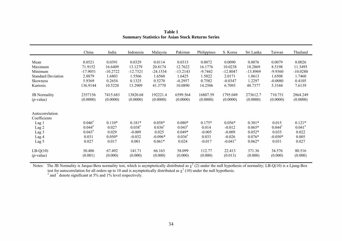
Table 1 Summary Statistics for Asian Stock Returns Series
China
India
Indonesia
Malaysia
Pakistan
Philippines
S. Korea
Sri Lanka
Taiwan
Thailand
0.0521
71.9152 0.0391
16.6409 0.0329
13.1279 0.0114
20.8174 0.0315
12.7622 0.0072
16.1776 0.0090
10.0238 0.0076
18.2869 0.0079 8.5198
0.0026 11.3495
-17.9051 2.8879 5.9369
136.9144
-10.2722 1.6803 0.2654
10.5220
-12.7321 1.5566 0.1325
13.2909
-24.1534 1.6560 0.5270
41.3770
-13.2143 1.6425 -0.2957 10.0890
-9.7442 1.5022 0.7582
14.2506
-12.8047 2.0171 -0.0347 6.7093
-13.8969 1.0613 1.2297
48.7377
-9.9360 1.6508 -0.0080 5.3344
-10.0280 1.7460 0.4105 7.6139
Mean Maximum Minimum Standard Deviation Skewness Kurtosis JB Normality (p-value) Autocorrelation Coefficients Lag 1 Lag 2 Lag 3 Lag 4 Lag 5 LB-Q(10) (p-value)
2357156 (0.0000)
0.046#
0.044#
0.043#
0.031 0.027
30.486 (0.001)
7415.683 (0.0000)
0.110* 0.027 0.029
0.050* 0.017
67.492 (0.000)
13820.68 (0.0000)
0.181* 0.038#
-0.009 -0.032 0.001
141.71 (0.000)
192221.4 (0.0000)
0.058* 0.036#
0.025 -0.096* 0.061*
66.163 (0.000)
6599.564 (0.0000)
0.080* 0.043#
0.049* 0.036#
0.024
58.099 (0.000)
16807.59 (0.0000)
0.175* 0.014 -0.005 0.033 -0.017
112.77 (0.000)
1795.049 (0.0000)
0.056* -0.012 -0.009 -0.026 -0.041#
22.413 (0.013)
273612.7 (0.0000)
0.301* 0.065* 0.052* 0.076* 0.062*
371.36 (0.000)
710.751 (0.0000)
0.015 0.044#
0.035 -0.050* 0.031
34.576 (0.000)
2864.249 (0.0000)
0.121* 0.041#
0.022 0.005 0.027
80.516 (0.000)
Notes: The JB Normality is Jarque-Bera normality test, which is asymptotically distributed as χ2 (2) under the null hypothesis of normality; LB-Q(10) is a Ljung-Box test for autocorrelation for all orders up to 10 and is asymptotically distributed as χ2 (10) under the null hypothesis.
# and * denote significant at 5% and 1% level respectively.
34

Table 2 Nonlinearity Test Results for Asian Stock Returns Series
China
India
Indonesia
Malaysia
Pakistan
Philippines
S. Korea
Sri Lanka
Taiwan
Thailand
0.112 0.148
0.000 0.000
0.000 0.000
0.000 0.000
0.000 0.000
0.009 0.011
0.000 0.000
0.003 0.003
0.000 0.000
0.000 0.000
McLeod-Li Test Using up to lag 20 Using up to lag 24 Bicorrelation Test Engle test Using up to lag 1 Using up to lag 2 Using up to lag 3 Using up to lag 4 Using up to lag 5 Tsay test BDS test ε /σ = 1; m=2 ε /σ = 1; m=3 ε /σ = 1; m=4 Bispectrum Test
0.002
0.043 0.022 0.017 0.018 0.023
0.006
0.000 0.000 0.000
0.0063
0.000
0.000 0.000 0.001 0.000 0.000
0.000
0.000 0.000 0.000
0.0516
0.000
0.000 0.000 0.000 0.000 0.000
0.003
0.000 0.000 0.000
0.0405
0.000
0.000 0.000 0.000 0.000 0.000
0.000
0.000 0.000 0.000
0.0063
0.000
0.000 0.000 0.000 0.000 0.000
0.000
0.000 0.000 0.000
0.0442
0.000
0.004 0.005 0.003 0.003 0.005
0.004
0.000 0.000 0.000
0.0134
0.000
0.000 0.000 0.000 0.000 0.000
0.000
0.000 0.000 0.000
0.1255
0.000
0.001 0.001 0.001 0.001 0.001
0.001
0.000 0.000 0.000
0.0063
0.000
0.000 0.000 0.000 0.000 0.000
0.000
0.002 0.000 0.000
0.4704
0.000
0.000 0.000 0.000 0.000 0.000
0.007
0.000 0.000 0.000
0.1445
Notes: With the exception of the bispectrum test, all the tests are carried out in the Nonlinear Toolkit of Patterson and Ashley (2000). These tests are applied to the residuals of an AR(p) model, in which the lag length is chosen to minimize the Schwartz Criterion. The statistics reported are bootstrap p-values with 1000 replications. On the other hand, the bispectrum test is implemented using the FORTRAN program that has incorporated the shuffle bootstrap approach proposed by Hinich et al. (2005). The reported statistics are the shuffle bootstrap p-values with 1000 replications.
35

Table 3 Significant H Statistics in Moving Time Windows Test
China
India
Indonesia
Malaysia
Pakistan
Philippines
S. Korea
Sri Lanka
Taiwan
Thailand
13
(20.97%)
9 (14.52%)
7 (11.29%)
11 (17.74%)
18 (29.03%)
9 (14.52%)
7 (11.29%)
23 (37.10%)
6 (9.68%)
8 (12.90%)
Total number of significant H windows Dates of significant H windows
3/12/92-5/20/92 7/30/92-10/7/92 7/15/93-9/22/93
11/17/94-1/25/95 8/24/95-11/1/95 3/21/96-5/29/96 3/6/97- 5/14/97 7/24/97-10/1/97 4/30/98-7/8/98 7/9/98-9/16/98
11/11/99-1/19/00 6/8/00-8/16/00 12/5/02-2/12/03
5/21/92-7/29/92 2/10/94-4/20/94 4/6/95-6/14/95 11/2/95-1/10/96 8/8/96-10/16/96
10/2/97-12/10/97 1/20/00-3/29/00
8/17/00-10/25/00 8/2/01-10/10/01
1/2/92-3/11/92 5/6/93-7/14/93 1/26/95-4/5/95 3/21/96-5/29/96 3/15/01-5/23/01
10/11/01-12/19/01 7/18/02-9/25/02
5/6/93-7/14/93 12/2/93-2/9/94 5/30/96-8/7/96 7/9/98-9/16/98 2/4/99-4/14/99 6/24/99-9/1/99 6/8/00-8/16/00 8/2/01-10/10/01
10/11/01-12/19/01 5/9/02-7/17/02 2/13/03-4/23/03
7/30/92-10/7/92 7/15/93-9/22/93 9/23/93-12/1/93 4/21/94-6/29/94
11/17/94-1/25/95 11/2/95-1/10/96 1/11/96-3/20/96 3/21/96-5/29/96
10/2/97-12/10/97 2/19/98-4/29/98
9/17/98-11/25/98 4/15/99-6/23/99
11/11/99-1/19/00 3/30/00-6/7/00 8/2/01-10/10/01 5/9/02-7/17/02 7/18/02-9/25/02 12/5/02-2/12/03
5/6/93-7/14/93 4/21/94-6/29/94
11/17/94-1/25/95 3/6/97-5/14/97 5/15/97-7/23/97
10/2/97-12/10/97 2/19/98-4/29/98 4/30/98-7/8/98 5/9/02-7/17/02
10/8/92-12/16/92 7/15/93-9/22/93 4/21/94-6/29/94 12/26/96-3/5/97 4/30/98-7/8/98
8/17/00-10/25/00 7/18/02-9/25/02
5/21/92-7/29/92 7/30/92-10/7/92 2/25/93-5/5/93 5/6/93-7/14/93 9/23/93-12/1/93 4/21/94-6/29/94 6/30/94-9/7/94 1/26/95-4/5/95 8/24/95-11/1/95 11/2/95-1/10/96 3/6/97-5/14/97 7/9/98-9/16/98 4/15/99-6/23/99 6/24/99-9/1/99 9/2/99-11/10/99
8/17/00-10/25/00 2/28/02-5/8/02 7/18/02-9/25/02 9/26/02-12/4/02 12/5/02-2/12/03 4/24/03-7/2/03 7/3/03-9/10/03
9/11/03-11/19/03
1/2/92-3/11/92 2/25/93-5/5/93 9/8/94-11/16/94 3/21/96-5/29/96 7/24/97-10/1/97 7/9/98-9/16/98
5/21/92-7/29/92 8/24/95-11/1/95 8/8/96-10/16/96
10/17/96-12/25/96 7/24/97-10/1/97 4/30/98-7/8/98 6/24/99-9/1/99 8/2/01-10/10/01
36

Figure 1: Time Series Plots for p-values of H Statistic (Taiwan)
0.000
0.100
0.200
0.300
0.400
0.500
0.600
0.700
0.800
0.900
1.000
1/2/
923/
12/9
25/
21/9
27/
30/9
210
/8/9
212
/17/
922/
25/9
35/
6/93
7/15
/93
9/23
/93
12/2
/93
2/10
/94
4/21
/94
6/30
/94
9/8/
9411
/17/
941/
26/9
54/
6/95
6/15
/95
8/24
/95
11/2
/95
1/11
/96
3/21
/96
5/30
/96
8/8/
9610
/17/
9612
/26/
963/
6/97
5/15
/97
7/24
/97
10/2
/97
12/1
1/97
2/19
/98
4/30
/98
7/9/
989/
17/9
811
/26/
982/
4/99
4/15
/99
6/24
/99
9/2/
9911
/11/
991/
20/0
03/
30/0
06/
8/00
8/17
/00
10/2
6/00
1/4/
013/
15/0
15/
24/0
18/
2/01
10/1
1/01
12/2
0/01
2/28
/02
5/9/
027/
18/0
29/
26/0
212
/5/0
22/
13/0
34/
24/0
37/
3/03
9/11
/03
Bootstrapped threshold = 0.0677
37
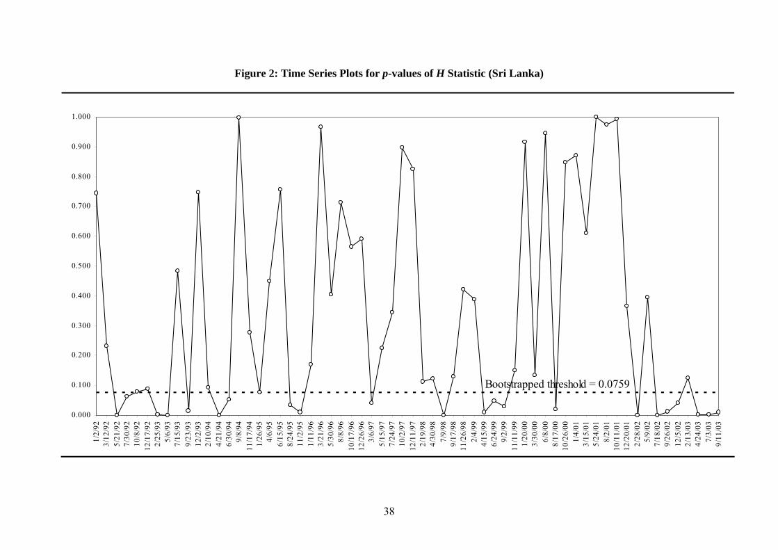
Figure 2: Time Series Plots for p-values of H Statistic (Sri Lanka)
0.000
0.100
0.200
0.300
0.400
0.500
0.600
0.700
0.800
0.900
1.000
1/2/
923/
12/9
25/
21/9
27/
30/9
210
/8/9
212
/17/
922/
25/9
35/
6/93
7/15
/93
9/23
/93
12/2
/93
2/10
/94
4/21
/94
6/30
/94
9/8/
9411
/17/
941/
26/9
54/
6/95
6/15
/95
8/24
/95
11/2
/95
1/11
/96
3/21
/96
5/30
/96
8/8/
9610
/17/
9612
/26/
963/
6/97
5/15
/97
7/24
/97
10/2
/97
12/1
1/97
2/19
/98
4/30
/98
7/9/
989/
17/9
811
/26/
982/
4/99
4/15
/99
6/24
/99
9/2/
9911
/11/
991/
20/0
03/
30/0
06/
8/00
8/17
/00
10/2
6/00
1/4/
013/
15/0
15/
24/0
18/
2/01
10/1
1/01
12/2
0/01
2/28
/02
5/9/
027/
18/0
29/
26/0
212
/5/0
22/
13/0
34/
24/0
37/
3/03
9/11
/03
Bootstrapped threshold = 0.0759
38