Demographic, Economic, and Political Determinants of
Land Development in the U. S.
Scott R. Templeton
259 Barre Hall
Department of Applied Economics and Statistics
Clemson University
Clemson SC 29634-0355
864-656-6680 (o), 864-656-5776 (f), and [email protected]
Selected short paper prepared for presentation at the Annual Meeting of the American
Agricultural Economics Association in Denver CO, July 1-4, 2004.
An earlier and less comprehensive version of this paper was presented at the 35th
Annual Meeting of the Southern Agricultural Economics Association, Mobile AL, 4
February 2003 and a related poster was presented at the AGU Chapman Conference on
Ecosystem Interactions with Land Use Change, Santa Fe NM, 17 June 2003. The Natural
Resource Conservation Service, USDA supported this research through Grant Agreement
No. 69-4639-1-0010. Ritu Sharma entered most of the demographic, economic, and
political data and used SAS for preliminary estimation. Basman Towfique entered land-
use data. Peter Berck, Hal Harris, Mark Henry, Karina Schoengold, and Webb Smathers
commented on preliminary results. I am responsible for any remaining error.
© 2004 by Scott R. Templeton. All rights reserved. Readers may make verbatim copies
of this document for non-commercial purposes by any means, provided that this
copyright notice appears on all such copies.
Abstract
Two reduced-form, econometric models of developed land area were estimated with the
data from the USDA’s National Resource Inventory and numerous other sources for 49
states during 1982-1997. In these linear and semi-quadratic fixed-effects models,
developed land area is smaller where the average real gas price or conservation reserve
program payment per enrolled acre during the previous five years is higher. This area
also decreases as the average share of lower-house Democrats or real per-capita
agricultural-mining production during the previous five years grows. Increases in a
state’s average population and average annual growth rate of real non-agricultural and
non-mining output per capita during the previous five years induce land development.
Policies that increase real CRP payments per enrolled acre, improve the real returns to
agriculture and mining, reduce population growth, or raise real gasoline prices are likely
to reduce land development.

Demographic, Economic, and Political Determinants of
Land Development in the U.S.
Introduction
Land development is ubiquitous in the U.S. The area of developed land increased
34%, from 73.246 million acres to 98.252 million acres, during 1982-1997 in the U.S.
except Alaska (NRCS, p. 36). Conversion of land from forestry, annual crop production,
and other ‘undeveloped’ uses to residential, commercial, and other ‘developed’ uses
accompanies economic growth. However, this land-use change can adversely affect
wildlife, water quality, and other natural resources (e.g., Heimlich and Anderson, pp. 31-
35). For example, land development led to a gross loss of 247,500 acres of Palustrine
and Estuarine wetlands in these 49 states during 1992-1997 (NRCS, p. 73). Vehicle
miles can increase with urban expansion (e.g., Kahn) and, by implication, emissions of
greenhouse-producing gases can too. For this and other reasons, urban and rural uses of
land affect climate in the U.S. (e.g., Bonan) and the world (e.g., Bounoua et al.). Models
of land-use change for continents and large countries have become important for
forecasting climate change (e.g., DeFries, Bounoua, and Collatz.).
Policies to reduce these negative externalities and forecasts of climate change as a
function of land-use change should be grounded in up-to-date, appropriately-scaled,
theoretically-motivated empirical models. In theory, land development depends on
population and income per capita (Muth, pp. 16-20) and growth rates of population
(Capozza and Helsey, p. 301), expected housing rents (Arnott and Lewis, p. 164), and
expected returns to urban use (Capozza and Li, p. 897). In early empirical analyses (e.g.,
Clawson; Zeimetz et al.; Vesterby and Heimlich), economic or demographic growth is
also the main determinant of land development but the quantitative impact in a
multivariate statistical model was not estimated. In recent empirical models of a land
owner’s decision of whether (e.g., Bockstael) or when (e.g., Irwin and Bockstael) to
develop a parcel of land, the quantitative effects of factors that determine differences in
financial returns to residential and agricultural uses of this parcel have been estimated.
Examples of these factors are zoning restrictions or distance of parcel to the nearest urban
center. In these models, however, the effects of population, economic production per
capita, associated growth rates, gas prices, and other factors that federal or state policy
makers can influence have not been estimated. Use of spatially explicit, parcel-level data
makes such estimation relatively difficult, if not prohibitively expensive.
In this paper the effects of demographic, economic, and political factors on statewide
land development throughout the U.S. except Alaska are estimated and analyzed.
Decomposition of real economic production and growth rates matters (e.g., Muth;
Norris). In theory, discounted rents and conversion costs depend on the real interest rate.
Moreover, in bid-offer models of land rent, distances to the central business district and,
more generally, the associated transport costs are the primary reason for changes in these
rents over space. Of course, land-use policies (e.g., Irwin and Bockstael) affect rents and
vary across state and time. Federal farm programs usually increase the profitability of
traditional agriculture. Finally, rents tend to be higher the more abundant and closer are
water resources to those properties (e.g., Bastian et al.).
Conceptual Framework
Our model of land development is a modification of Irwin and Bockstael’s model.
Assume that perfectly competitive landowners maximize the net present financial value
-2-
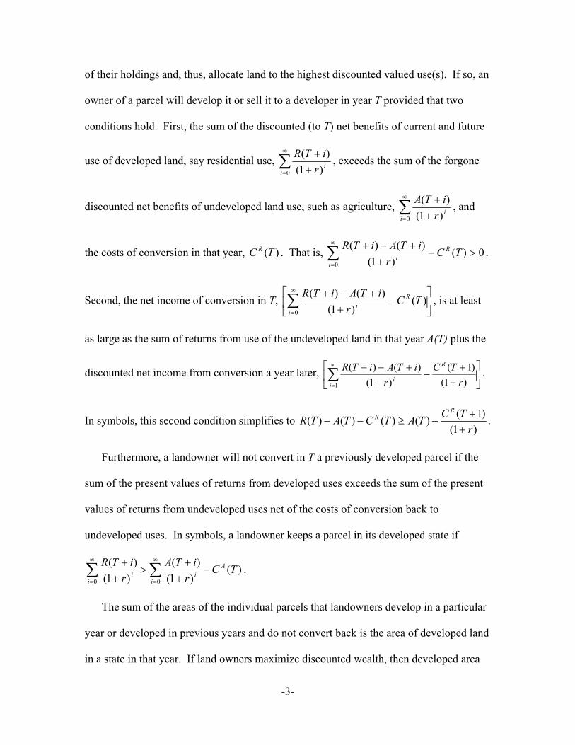
of their holdings and, thus, allocate land to the highest discounted valued use(s). If so, an
owner of a parcel will develop it or sell it to a developer in year T provided that two
conditions hold. First, the sum of the discounted (to T) net benefits of current and future
use of developed land, say residential use, ∑ , exceeds the sum of the forgone
discounted net benefits of undeveloped land use, such as agriculture,
∞
= ++
0 )1()(
iiriTR
∑∞
= ++
0 )1()(
iiriTA , and
the costs of conversion in that year, C . That is, )(TR 0)()1(
)()(0
>−+
+−+∑∞
=
TCr
iTAiTR R
ii .
Second, the net income of conversion in T,
−
++−+∑
∞
=
)()1(
)()(0
TCr
iTAiTR R
ii , is at least
as large as the sum of returns from use of the undeveloped land in that year A(T) plus the
discounted net income from conversion a year later,
++
−+
+−+∑∞
= )1()1(
)1()()(
1 rTC
riTAiTR R
ii
.
In symbols, this second condition simplifies to )1(
)1()()()()(r
TCTATCTATRR
R
++
−≥−− .
Furthermore, a landowner will not convert in T a previously developed parcel if the
sum of the present values of returns from developed uses exceeds the sum of the present
values of returns from undeveloped uses net of the costs of conversion back to
undeveloped uses. In symbols, a landowner keeps a parcel in its developed state if
)()1(
)( )1(
)(00
TCr
iTAr
iTR A
ii
ii −
++
>++ ∑∑
∞
=
∞
=
.
The sum of the areas of the individual parcels that landowners develop in a particular
year or developed in previous years and do not convert back is the area of developed land
in a state in that year. If land owners maximize discounted wealth, then developed area
-3-
depends on undiscounted current and future returns to developed and undeveloped uses
of parcels, conversion costs, interest rates, and land-use regulations.
Variables and Data Sources
The U. S. Department of Agriculture’s Natural Resources Conservation Service has
conducted the National Resources Inventory (NRI) every five years since 1982. This
inventory entails periodic aerial sampling of hundreds of thousands of parcels with
ground truthing to estimate, among other things, the area of developed land for each state
of the U.S. except Alaska (NRCS, p. 3). Sampled and estimated areas have reflected
growing season conditions in individual states in those years (NRCS, p. 3).
The Natural Resources Conservation Service has not collected financial data from
individual owners of parcels in their samples. Moreover, to keep identities of parcel
owners confidential, NRCS does not release longitude and latitude coordinates of the
exact locations of sampled parcels. Hence, data on financial returns from uses of specific
parcels, conversion costs, discount rates of individual owners in the NRI sample, and
non-pecuniary benefits and costs to owners of these uses cannot be collected. However,
data on variables that affect these returns, costs, and discount factors are available.
Table 1 presents descriptive statistics for the area of developed land and exogenous
variables that affect land development. DEVAREA represents the area of non-federally
owned large urban and built-up areas, small built-up areas, and rural transportation land
in a state in 1982, 1987, 1992, and 1997 (NRCS, p. 82). Urban and built-up areas include
residential, industrial, commercial, and institutional land, construction sites, railroad
yards, cemeteries, airports, golf courses, landfills, sewage treatment plants, and urban
roadways (NRCS, p. 88). Rural transportation land includes all highways, roads,
-4-
railways, and other rights-of-way outside of urban and built-up areas (NRCS, p. 86).
To reflect the periodic, during-the-year timing of the NRI and non-instantaneous land
conversion, demographic, economic, and political variables were constructed to
summarize conditions during the five or four years prior to the year in which areas of
developed land were sampled and estimated. This construction also eliminates the
possibility that these variables could be endogenous. For example, POP represents the
mean of the mid-year populations in a state for 1977-1981, 1982-1986, 1987-1991, and
1992-1996 (Census Bureau 2002, 1996, 1995). POPGR is the mean of the annual growth
rates of state population for 1978-1981, 1982-1986, 1987-1991, and 1992-1996.
Traditional agriculture and mining are the primary economic activities that use
undeveloped land. To account for these differences in the location of productive
activities and, thus, potential impacts on rents, economic production per capita is
separated into real agricultural and mining output per capita and all other real production
per capita. In particular, AGMINEPC and NANMPC represent the means of real (1996
$s) agricultural and mining output per capita of agricultural and all other production per
capita in a state for the five years prior to 1982, 1987, 1992, and 1997 (BEA). Real
agricultural production per capita, by construction and data availability, includes real
output of forestry and fishing. AGMGR and NANMGR are the means of the annual
growth rates of real agricultural and mining output per capita and all other real production
per capita for 1978-1981, 1982-1986, 1987-1991, and 1992-1996.
The Federal Home Mortgage Corporation provided data on the fixed interest rates for
30-year conventional mortgages for the U.S per year for 1977-1997 (FHMC). The real
interest rate in a particular state and year was calculated as this nominal interest rate for
-5-
the nation in that year minus the state’s inflation rate in that year. A state’s inflation rate
equals the ratio of state’s price index in a given year to the index in the previous year
minus one. The price index equals the state’s nominal gross state product divided by its
real (1996 $s) gross state product. SINTRATE represents the mean real interest rate for
30-year conventional mortgages in a state for ‘78-‘81, ‘82-‘86, ‘87-‘91, and ‘92-‘96.
The Energy Information Administration of the US Department of Energy publishes
annual, statewide data on the nominal price of motor gasoline, measured in dollars per
million British Thermal Units (EIA). The real (1996 $s) price of motor gasoline equals
the nominal price in a particular state and year divided by the state’s price index for that
year. GASPRICE represents the average real price of motor gasoline in a state for the
five years prior to 1982, 1987, 1992, and 1997.
There is no available published information that summarizes the degree of zoning in a
particular state and year. However, reputations and legislative records of the two major
political parties suggest differences in their approach to regulation (Friedman).
SHAREDEM equals the mean of the shares of Democrats in the lower house of a state’s
legislature for the five years prior to 1982, 1987, 1992, and 1997. These shares were
calculated with data on the number of state legislators by political party affiliation after
each state election (Census Bureau 2001, 1999, 1992, 1986, and 1984).
Another political determinant is the Conservation Reserve Program (CRP). The CRP
provides farmers with rental payments and cost-share assistance to plant trees or other
resource-conserving vegetative covers to improve the quality of water, control soil
erosion, and enhance wildlife habitat (Farm Service Agency). CRPAYPA and
CRPAREA represent average real (1996 $s) net outlay per enrolled acre and the enrolled
-6-
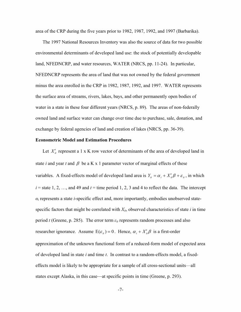
area of the CRP during the five years prior to 1982, 1987, 1992, and 1997 (Barbarika).
The 1997 National Resources Inventory was also the source of data for two possible
environmental determinants of developed land use: the stock of potentially developable
land, NFEDNCRP, and water resources, WATER (NRCS, pp. 11-24). In particular,
NFEDNCRP represents the area of land that was not owned by the federal government
minus the area enrolled in the CRP in 1982, 1987, 1992, and 1997. WATER represents
the surface area of streams, rivers, lakes, bays, and other permanently open bodies of
water in a state in these four different years (NRCS, p. 89). The areas of non-federally
owned land and surface water can change over time due to purchase, sale, donation, and
exchange by federal agencies of land and creation of lakes (NRCS, pp. 36-39).
Econometric Model and Estimation Procedures
Let X ′ represent a 1 x K row vector of determinants of the area of developed land in
state i and year t and
it
β be a K x 1 parameter vector of marginal effects of these
variables. A fixed-effects model of developed land area is Y ititiit X εβα +′+= , in which
i = state 1, 2, …, and 49 and t = time period 1, 2, 3 and 4 to reflect the data. The intercept
αi represents a state i-specific effect and, more importantly, embodies unobserved state-
specific factors that might be correlated with Xit, observed characteristics of state i in time
period t (Greene, p. 285). The error term εit represents random processes and also
researcher ignorance. Assume 0)(E =itε . Hence, βα iti X ′+ is a first-order
approximation of the unknown functional form of a reduced-form model of expected area
of developed land in state i and time t. In contrast to a random-effects model, a fixed-
effects model is likely to be appropriate for a sample of all cross-sectional units—all
states except Alaska, in this case—at specific points in time (Greene, p. 293).
-7-

Fixed-effects models of developed land area were estimated with the ordinary least
squares (OLSQ) command in Time Series Processor (TSP), Version 4.5 (Hall and
Cummins). A fixed-effect model with 13 exogenous variables and the square of each of
these variables was initially estimated to detect possible non-linear effects, such as
Vesterby and Heimlich (p. 287) found for population. Squared variables with
insignificant effects were dropped and the resultant semi-quadratic model was re-
estimated. A fixed-effect, linear-in-variables model was also estimated.
Given evidence from Lagrange multiplier tests in favor of H1: var(εit) = =
var(ε
22ji σσ ≠
jt), heteroskedastic-consistent standard errors were calculated with the Eicker-White
estimator divided by (T-K)/T (Hall and Cummins, p. 185). In models with n fixed effects
for all cross-sectional units, K other explanatory variables, and T time periods, the
appropriate divisor in the Eicker-White estimator is nTKnnT −− , or 196K−147 for
these data. Preceded by the frequency statement FREQ (PANEL, T=4), OLSQ correctly
calculated the Durbin-Watson statistic, ( )∑ ∑∑ ∑= == =
−
=
49
1
4
1
49
1
4
21
i tit
i titit eeed
2 , for these
balanced panel data. Given evidence from Durbin-Watson tests in favor of first-order
autocorrelation, H1: ρ > 0, and, thus, cov [εt, εt-1] ≠ 0, Prais-Winsten transformations of
the dependent variable were regressed on identical transformations of state-specific
intercepts and exogenous variables to correct for these non-spherical disturbances.
-8-
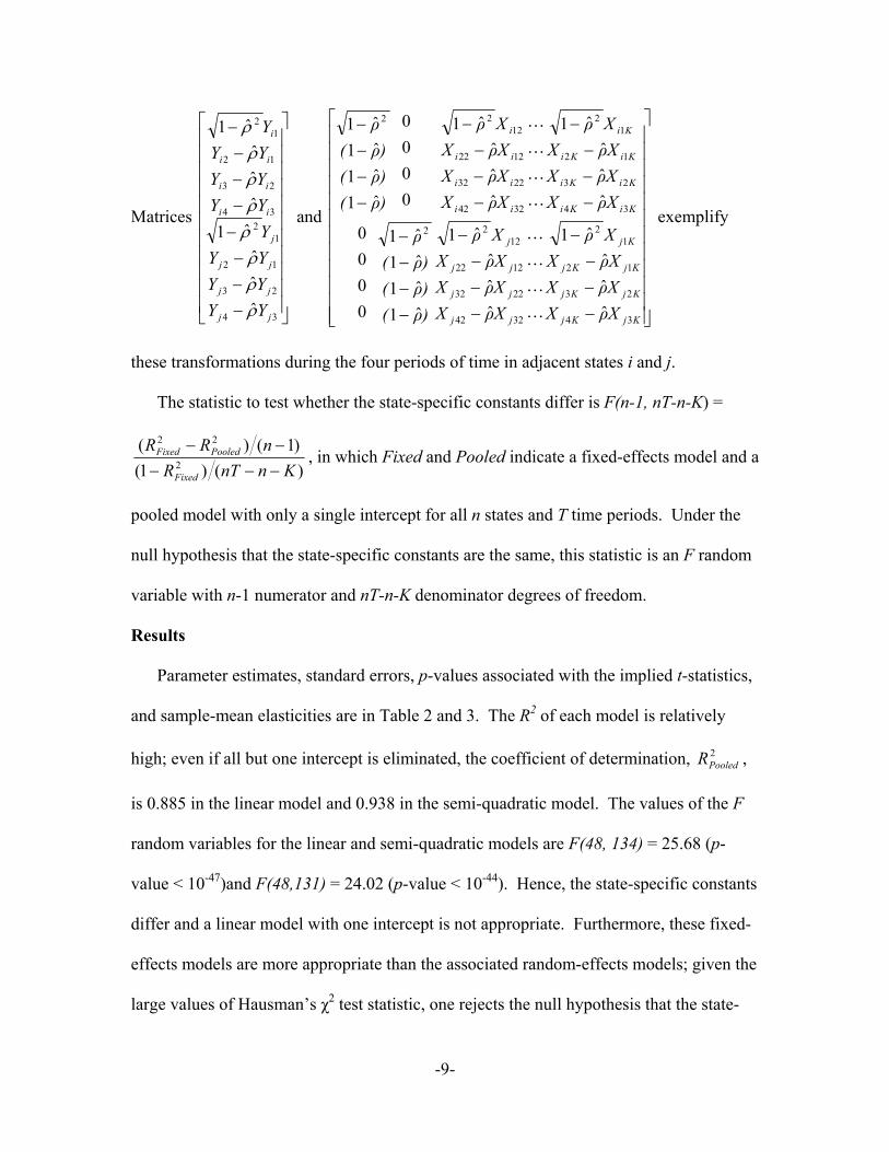
Matrices
−−−−−−−−
34
23
12
12
34
23
12
12
ˆˆˆ
ˆ1ˆˆˆ
ˆ1
jj
jj
jj
j
ii
ii
ii
i
YYYYYYYYYYYYYY
ρρρρρρρρ
and
−−−
−
−−−
−
−−−−
−−−
−
−−−
−
−−−−
KjKj
KjKj
KjKj
Kj
jj
jj
jj
j
KiKi
KiKi
KiKi
Ki
ii
ii
ii
i
XρXXρXXρX
Xρ
XρXXρXXρXXρ
)ρ()ρ()ρ(ρ
XρXXρXXρXXρ
XρXXρXXρXXρ
)ρ()ρ()ρ(ρ
34
23
12
12
3242
2232
1222
1222
34
23
12
12
3242
2232
1222
1222
ˆˆˆ
ˆ1
ˆˆˆ
ˆ1
ˆ1ˆ1ˆ1ˆ1
0000
ˆˆˆ
ˆ1
ˆˆˆ
ˆ1
0000
ˆ1ˆ1ˆ1ˆ1
K
K
K
K
K
K
K
K
exemplify
these transformations during the four periods of time in adjacent states i and j.
The statistic to test whether the state-specific constants differ is F(n-1, nT-n-K) =
)()1()1()(
2
22
KnnTRnRR
Fixed
PooledFixed
−−−−−
, in which Fixed and Pooled indicate a fixed-effects model and a
pooled model with only a single intercept for all n states and T time periods. Under the
null hypothesis that the state-specific constants are the same, this statistic is an F random
variable with n-1 numerator and nT-n-K denominator degrees of freedom.
Results
Parameter estimates, standard errors, p-values associated with the implied t-statistics,
and sample-mean elasticities are in Table 2 and 3. The R2 of each model is relatively
high; even if all but one intercept is eliminated, the coefficient of determination, ,
is 0.885 in the linear model and 0.938 in the semi-quadratic model. The values of the F
random variables for the linear and semi-quadratic models are F(48, 134) = 25.68 (p-
value < 10
2PooledR
-47)and F(48,131) = 24.02 (p-value < 10-44). Hence, the state-specific constants
differ and a linear model with one intercept is not appropriate. Furthermore, these fixed-
effects models are more appropriate than the associated random-effects models; given the
large values of Hausman’s χ2 test statistic, one rejects the null hypothesis that the state-
-9-
specific constants are uncorrelated with the other exogenous variables in favor of the
alternative that these constants are correlated. In terms of adjusted R2, the log of the
likelihood function, and Schwarz’s criterion, the semi-quadratic model variables fits the
data slightly better than the linear model does. Variance inflation factors (VIFs) of the
untransformed exogenous variables did not indicate serious multicollinearity; two of the
variables had VIFs between 2.2 and 2.6 and the other nine had VIFs between 1.2 and 2.0.
The positive effect of POP in both models and negative effect of POPSQ in the semi-
quadratic model are significant. In the semi-quadratic model, each additional person in a
state during the previous five years induces, on average, an additional 0.422 acres of
developed land. A one percent increase in the average previous five-year population
leads to a subsequent 1.2% average increase in developed land area.
The negative effect of average real agricultural and mining output per capita in the
previous five years, AGMINEPC, is statistically significant and similar in both models.
An increase of $100 in AGMINEPC leads to approximately 6,000 fewer acres of
developed land. A 10% increase in average real agricultural and mining output per capita
in the previous five years leads to a 0.7% decrease in developed land area.
The positive effect of average real non-agricultural and non-mining output per capita
output in the previous five years, NANMPC, is statistically significant in the semi-
quadratic model, albeit at the 92.5% confidence level. In particular, an increase of $100
in average real per capita output other than agriculture or mining in the previous five
years induces 1,434 more acres of developed land. In other words, a 10% increase in
NANMPC induces a 3.9% increase in developed land area. The average annual rate of
growth of real non-agricultural and non-mining output per capita in the previous five
-10-
years, NANMGR, also encourages land development. The p-value associated with the t-
statistic is smaller and the parameter estimate is larger in the semi-quadratic than the
linear model. In particular, an increase of one percentage point in NANMGR leads to an
increase of 23,309 acres of developed land in the semi-quadratic model.
The negative effect of GASPR is statistically significant in both models, although the
absolute value of the effect and the confidence level are lower in the linear model. In the
semi-quadratic model an increase of $1 in the previous five-year average price per
million BTUs of motor gas--an approximate increase of $.124 per gallon--leads to a
decrease in developed area, on average, of 41,617 acres. A 10% increase in GASPR
subsequently reduces developed land area by 6.0%, on average.
Political variables matter too. In two of three cases, the qualitative effects and p-
values are robust to the model specification. In the semi-quadratic model, developed land
area is 5,965 acres smaller, on average, in a state where the previous five-year average
share of Democrats in the state’s lower legislative house is one percentage point higher.
An increase of $10 in the previous five-year average real conservation reserve program
payment per enrolled acre, CRPAYPA, leads to 2,486 fewer acres of developed land. A
10% increase in CRPAYPA induces a 0.09% decrease in the area of developed land. The
effect of CRPAREA becomes significant at a high level of confidence in the semi-
quadratic model. The area of developed land is 189 acres smaller, on average, in a state
with 1000 more acres enrolled in the CRP during the previous five years. A 10%
increase in this area leads to a 0.38% decrease, on average, in developed land area.
Discussion
The signs and magnitudes of the parameter estimates compare reasonably well with
-11-
results from previous research, are consistent with economic theories about land rents and
owners of land who allocate it to the highest present-valued use(s), or both.
Marginal consumption of urban land in 135 fast-growth counties of the U.S. during
the early 1970s to the early 1980s was 0.47 additional acres per additional household, or
0.216 acres per additional person (Vesterby and Heimlich, p. 285). The urban area in
those counties that was estimated with land-use data from aerial photographs was 0.5
million acres smaller than the area in those same counties that fit the Census Bureau’s
population-based definition of urban (Vesterby and Heimlich, p. 282). Marginal
consumption of urban land--defined by the Census Bureau, calculated with the USDA’s
Major Land Uses data, and also called the urban land-use coefficient--was 0.69 acres per
additional person during 1974-1987 in the continental U. S. (Reynolds, p. 277).
‘Urban area’ for Census purposes, however, is smaller than the National Resource
Inventory’s developed land area. In 1997, for example, urban area was 62 million acres,
which was 36 million acres, or 37%, less than developed land area (Heimlich and
Anderson, p. 12). Developed land area includes rural transportation land and large, often
scattered, residential lots in rural areas. Development of these lots in rural areas,
particularly lots 10 acres or larger, grew during the economic expansion of the 1990s
(Heimlich and Anderson, pp. 13-14). Although differences in developed and urban land
areas make direct comparisons of urban land-use coefficients impossible, the estimated
increase of developed land area of 0.422 acres for each additional person in the previous
five years during 1982-1997 seems credible.
Increases in developed land area that get smaller as population grows imply that rents
grow more for uses of developed land than for uses of undeveloped land, but these
-12-
positive differences get smaller as population grows. This differential pattern of rent
increases is consistent with one or more of the following two hypotheses. First, demand
increases proportionately more for uses of developed land than for uses of undeveloped
land but the difference gets smaller as population grows. In other words, the population
elasticity of demand for uses of developed land exceeds that for uses of undeveloped land
but the excess becomes smaller as population grows. Second, the price elasticity of
supply of land for undeveloped uses exceeds that for developed uses. In particular,
farmers are more willing or able to substitute fertilizers, pesticides, new varieties of
seeds, and other ‘modern’ inputs for land to increase production as rents for undeveloped
land increase than developers are willing or able to substitute vertical space and
horizontal space-saving inputs for land to produce sites for residential, commercial,
industrial and other ‘urban’ activities as rents for developed land increase.
Increases in the previous five-year average real agricultural and mining output per
capita do not imply increases in the previous five-year average real gross state product
per capita. The sample correlation coefficient between real gross state product per capita
and real agricultural and mining output per capita is only 0.07 and no linear association
between the two variables exists (p-value = 0.35). Increases in the federal government’s
agricultural price supports, growth in the demand for a state’s agricultural or mining
exports, or weather-related decreases in supply of agricultural and mining products with
price inelastic demand would lead to increases in real agricultural and mining output per
capita. Hence, increases in the previous five-year average real agricultural and mining
output per capita, ceteris paribus, most likely imply increases in real net earnings in the
present and, given constant growth rates, in the future from uses of undeveloped land
-13-
relative to developed land. Increases in the average conservation-reserve-program
payments per acre of enrolled land in the previous five years definitely imply increases in
real returns to owners of agricultural and timber land for the length of the CRP contract.
As real returns for uses of undeveloped land increase, some of this land that would
otherwise be converted to ‘urban’ uses is not developed.
Real non-agricultural and non-mining output per capita constitutes, on average, 95%
of real gross state product per capita. The sample correlation coefficient between these
two variables is 0.96 and the linear association between them is strongly positive (p-value
< 10-107). Hence, increases in real non-agricultural and non-mining output per capita
imply increases in income per capita in a state. The income elasticity of demand for the
highest-valued developed use of land along the spatial margin probably exceeds the
income elasticity of demand for the highest-valued undeveloped use of that land. For
example, most estimates indicate that the income elasticity of demand for housing in the
long run exceeds that for food (e.g., Deaton and Muellbauer, pp. 319-320; Muth, p. 19).
If so, increases in real non-agricultural and non-mining output per capita and its growth
rate imply proportionately greater increases in real current and future rents for uses of
developed land than rents for uses of undeveloped land.
In theory (e.g., Capozza and Helsey, p. 297) and empirical analyses (e.g., Bockstael,
p. 1176), housing prices usually decline as residential locations get farther from the
central business district, town center, or highway because commuting costs increase with
distance. Commuting costs also increase with the real price of gas. Although prices of
land for developed and undeveloped uses will decrease as transport costs increase, the
decrease in the price of land for developed uses will tend to be more pronounced because
-14-
commuting tends to be more time-intensive for users of developed land than users of
undeveloped land. For example, people typically commute four to six days per week
whereas farmers transport produce a few times per year. As a result, less land is
converted to developed uses as real gas prices increase. In other words, for a given
population, the area of developed land decreases as the real price of gas increases
because, to economize on commute costs, people choose to live and work closer together
and, thereby, create denser uses of developed land. Increases in gas prices also imply
increases in the cost of converting undeveloped land into developed land.
Zoning and other land-use policies affect the returns to uses of undeveloped and
developed land. As the share of Democrats in the lower legislative house increases, local
government officials might be more likely to regulate land use because these officials are
more likely to be Democrats themselves or, at least, the voting public is more likely to
support such policies. In general, Democrats regulate the economy and its environmental
impacts more than Republicans do (Friedman). As prohibitions and inhibitions on land
development increase, future real returns to developed uses of currently undeveloped land
decrease and the amount of land that is converted to urban uses decreases as well.
Implications for Research and Policy
Although these two models explain a relatively large proportion of the variation in
developed land area across states during 1982-1997, their specifications can be improved.
None of the exogenous variables served exclusively as a proxy for these costs. Forested
land and steep land are more costly to develop than crop land and flat land are
(Bockstael, pp. 1176-1177). The NRI contains information on the area of forest and the
erodibility index of cropland in each state in each of the four years of observation.
-15-
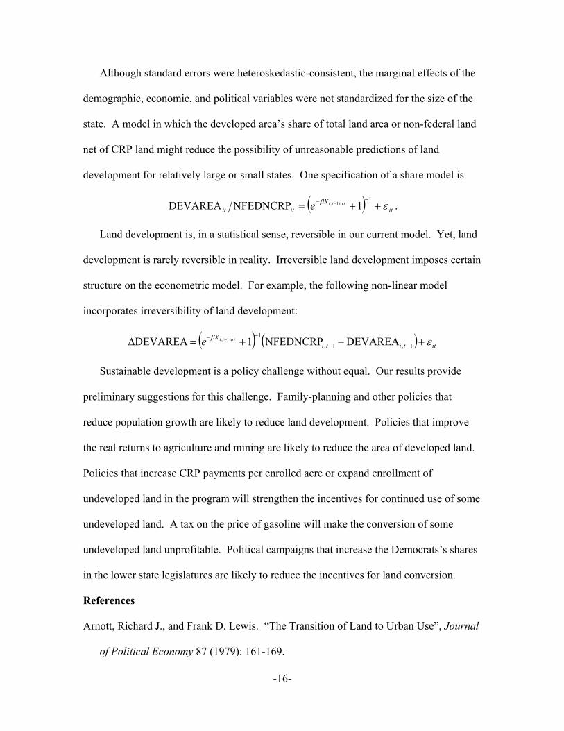
Although standard errors were heteroskedastic-consistent, the marginal effects of the
demographic, economic, and political variables were not standardized for the size of the
state. A model in which the developed area’s share of total land area or non-federal land
net of CRP land might reduce the possibility of unreasonable predictions of land
development for relatively large or small states. One specification of a share model is
( ) itX
ititttie εβ ++=
−− −1
1NFEDNCRPDEVAREA to1, .
Land development is, in a statistical sense, reversible in our current model. Yet, land
development is rarely reversible in reality. Irreversible land development imposes certain
structure on the econometric model. For example, the following non-linear model
incorporates irreversibility of land development:
( ) ( ) ittitiX ttie εβ +−+=∆ −−
−− −1,1,
1DEVAREANFEDNCRP1DEVAREA to1,
Sustainable development is a policy challenge without equal. Our results provide
preliminary suggestions for this challenge. Family-planning and other policies that
reduce population growth are likely to reduce land development. Policies that improve
the real returns to agriculture and mining are likely to reduce the area of developed land.
Policies that increase CRP payments per enrolled acre or expand enrollment of
undeveloped land in the program will strengthen the incentives for continued use of some
undeveloped land. A tax on the price of gasoline will make the conversion of some
undeveloped land unprofitable. Political campaigns that increase the Democrats’s shares
in the lower state legislatures are likely to reduce the incentives for land conversion.
References
Arnott, Richard J., and Frank D. Lewis. “The Transition of Land to Urban Use”, Journal
of Political Economy 87 (1979): 161-169.
-16-
Barbarika, Alexander. “Estimated Cumulative CRP Enrollment, by Year and State
(Acres)” and “Net CRP Outlays”, Unpublished Data, Farm Service Agency, U. S.
Dept. of Agriculture, Sept. - Oct. 2003, [email protected].
Bastian, Chris T., Donald M. McLeod, Matthew J. Germino, William A. Reiners, and
Benedict J. Blasko. “Environmental Amenities and Agricultural Land Values: A
Hedonic Model Using Geographic Information Systems Data”, Ecological Economics
40 (2002): 337-49.
Bockstael, Nancy E. “Modeling Economics and Ecology: The Importance of a Spatial
Perspective”, American Journal of Agricultural Economics 78 (Dec. 1996): 1168-
1180.
BEA. “Gross State Product (millions of current dollars)” and “Quantity Indexes for Real
GSP (1996=100.0)” for 1) Agriculture, Forestry, and Fishing, 2) Mining, and 3) Total
Gross State Product. Gross State Product Data, Regional Accounts Data, Bureau of
Economic Analysis, U.S. Department of Commerce, 2003.
http://www.bea.gov/bea/regional/gsp.
Bonan, Gordon B. “Frost Followed the Plow: Impacts of Deforestation on the Climate of
the United States”, Ecological Applications 9 (1999): 1305-1315.
Bounoua L., Ruth S. Defries, G.James Collatz and Piers J. Sellers, and H. Khan. “Effects
of Land Cover Conversions on Surface Climate”, Climatic Change 52 (2002): 29-64.
Capozza, Dennis and Yuming Li. “The Intensity and Timing of Investment: The Case of
Land”, American Economic Review 84 (Sept. 1994): 889-904.
Capozza, Dennis R. and Robert W. Helsley. “The Fundamentals of Land Prices and
Urban Growth”, Journal of Urban Economics 26 (1989): 295-306.
-17-
Census Bureau. “Table CO-EST2001-12-00 - Time Series of Intercensal State
Population Estimate, April 1, 1990 to April 1, 2000”. Population Estimates Program,
Population Division, U.S. Census Bureau, Washington DC, 2002.
http://eire.census.gov/popest/data/counties/tables/CO-EST2001-12/CO-EST2001-12-
00.php.
Census Bureau. “Table No. 395 Composition of States Legislatures by Political Party
Affiliation: 1994 to 2000”, Statistical Abstract of the United States: 2001, 121th Ed.
Bureau of the Census, Economics and Statistics Administration, Department of
Commerce, Washington DC, 2001, pg. 248.
Census Bureau. “Table No. 479 Composition of States Legislatures by Political Party
Affiliation: 1990 to 1996”, Statistical Abstract of the United States: 1999, 119th Ed.
Bureau of the Census, Economics and Statistics Administration, Department of
Commerce, Washington DC, 1999, pg. 296.
Census Bureau. “Intercensal Estimates of the Total Resident Population of States: 1980
to 1990”. Population Estimates Branch, U.S. Bureau of the Census, 1996.
http://www.census.gov/population/estimates/state/stts/st8090ts.txt.
Census Bureau. Intercensal Estimates of the Total Resident Population of States: 1970 to
1980. Population Estimates Branch, U.S. Bureau of the Census, 1995.
http://www.census.gov/population/estimates/state/stts/st7080ts.txt.
Census Bureau. “Table No. 430 Composition of States Legislatures by Political Party
Affiliation: 1984 to 1990”, Statistical Abstract of the United States: 1992, 112th Ed.
Bureau of the Census, Economics and Statistics Administration, Department of
Commerce, Washington DC, 1992, pg. 266.
-18-
Census Bureau. “Table No. 426 Composition of States Legislatures by Political Party
Affiliation: 1978 to 1984”, Statistical Abstract of the United States: 1986, 106th Ed.
Bureau of the Census, Economics and Statistics Administration, Department of
Commerce, Washington DC, 1986, pg. 251.
Census Bureau. “Table No. 432 Composition of States Legislatures by Political Party
Affiliation: 1994 to 2000”, Statistical Abstract of the United States: 1984, 104th Ed.
Bureau of the Census, Economics and Statistics Administration, Department of
Commerce, Washington DC, 1984, pg. 260.
Clawson, Marion. Suburban Land Conversion in the United States: An Economic and
Governmental Process. The John Hopkins University Press for Resources for the
Future, Inc., Baltimore MD, 1971.
Deaton, Angus and John Muellbauer. An Almost Ideal Demand System, American
Economic Review 70 (June 1980): 312-326.
Defries, Ruth S., Lahouari Bounoua, and G. James Collatz. “Human Modification of the
Landscape and Surface Climate in the Next Fifty Years”, Global Change Biology 8
(2002): 438-458.
EIA. State Energy Price and Expenditure Report 1999. Energy Information
Administration, Office of Energy Markets and End Use, U.S. Department of Energy,
Washington, DC, 2001. http://www.eia.doe.gov/emeu/states/_price_multistate.html.
Farm Service Agency. “Conservation Reserve Program: Fact Sheet”, US Dept. of
Agriculture, April 2003,
http://www.fsa.usda.gov/pas/publications/facts/html/crp03.htm
FHMC. “Selected Interest Rates: H.15, Fixed Rates for 30-Year Conventional
-19-
Mortgages”, Federal Reserve Statistical Release, Federal Home Mortgage
Corporation, 2003. http://www.federalreserve.gov/releases/h15/data/a/cm.txt.
Friedman, David. “The Politics of Growth”, Los Angeles Times, 17 Sept. 2000.
Greene, William H. “Chapter 13: Models for Panel Data”, Econometric Analysis, 5th
Edition, Prentice Hall, Upper Saddle River NJ, 2003, pgs. 588-589.
Hall, Bronwyn H. and Clint Cummins. Reference Manual, Time Series Processor,
Version 4.5, TSP International, Palo Alto CA, April 1999.
Heimlich, Ralph E. and William D. Anderson. Development at the Urban Fringe and
Beyond: Impacts on Agriculture and Rural Land, Agricultural Report No. 803,
Economic Research Service, USDA, Washington DC, June 2001.
http://www.ers.usda.gov/publications/aer803.
Irwin, Elena G. and Nancy E. Bockstael. “Interacting Agents, Spatial Externalities, and
the Endogenous Evolution of Residential Land Use Patterns”, Journal of Economic
Geography 2 (2002): 31-54.
Kahn, Matthew E. “The Environmental Impact of Suburbanization”, Journal of Policy
Analysis and Management 19 (2000): 569-586.
Muth, Richard F. “Economic Change and Rural-Urban Land Conversions”,
Econometrica 29 (Jan. 1961): 1-23.
Norris, Patricia E. “Land-Use Change, Resource Competition, and Conflict: Discussion”,
Journal of Agriculture and Applied Economics 33 (Aug. 2001): 311-314.
NRCS. Summary Report 1997 National Resources Inventory (revised December 2000).
Natural Resources Conservation Service, U. S. Department of Agriculture in
cooperation with Iowa State University Statistical Laboratory. 2000.
-20-
http://www.nrcs.usda.gov/technical/NRI/1997/summary_report/index.html.
Reynolds, John E. “Land Use Change and Competition in the South”, Journal of
Agricultural and Applied Economics 33 (Aug. 2001): 271-281.
Vesterby, Marlow and Ralph E. Heimlich. “Land Use and Demographic Change: Results
from Fast-Growth Counties”, Land Economics 67 (Aug. 1991): 279-291.
Zeimetz, K.A., E. Dillon, E.E. Hardy and R. C. Otte. Dynamics of Land Use in Fast
Growth Areas. Agricultural Economic Report No. 325, Economic Research Service,
United States Department of Agriculture, Washington, DC, 1976.
-21-
Table 1: Descriptive Statistics
Variable Mean Std.
Deviation Minimum Maximum
DEVAREA (1,000 acres) 1,717 1,345 149 8,567
POP (1,000 people) 4,929 5,208 452 31,490
AGMINEPC (1996$/person) 1,090.18 1,372.86 98.31 10,028.25
NANMPC (1996$/person) 22,059.55 4,643.75 13,618.82 37,340.56
POPGR (percentage pts.) 1.09 1.12 -1.50 5.74
AMGR (percentage pts.) 3.20 5.01 -6.99 30.73
NANMGR (percentage pts.) 1.90 1.31 -2.73 5.49
SINTRATE (percentage pts.) 6.40 2.15 -2.84 14.03
GASPRICE (1996$/million BTUs
or ≈1996 $s/gallon)
11.68
1.45
2.12
0.26
8.12
1.01
17.99
2.23
SHAREDEM (percentage pts.) 59.0 17.6 22.0 96.8
CRPAYPA ($s/acre) 31.78 48.51 0.00 401.57
WATER (1,000 acres) 1,010 923 52 4,045
CRPAREA (1,000 acres) 316 676 0 4,042
NFEDNCR (1,000 acres) 30,029 24,423 655 164,594
-22-
Table 2: Linear Model of Developed Land Area
Variable Estimated
Coefficient Std. Error t-statistic p-value
Elasticity of
Sig. Variable
POP 0.223 0.058 3.858 [.000] 0.615
AGMINEPC -0.058 0.033 -1.786 [.076] -0.069
NANMPC 0.014 0.010 1.441 [.152]
POPGR 5.127 16.858 0.304 [.762]
AMGR -0.262 2.167 -0.121 [.904]
NANMGR 14.831 7.665 1.935 [.055] 0.033
SINRATE -0.890 5.078 -0.175 [.861]
GASPR -30.163 13.955 -2.161 [.032] -0.436
SHRDEM -10.544 2.458 -4.289 [.000] -0.738
CRPAYPA -0.309 0.149 -2.077 [.040] -0.011
WATER 0.220 0.310 0.708 [.480]
CRPAREA 0.037 0.068 0.547 [.585]
NFEDNCRP -0.006 0.058 -0.111 [.912]
ρ̂ , Adjusted R2, Log Likelihood, and Schwarz Criterion 49 State
CONSTANTS 0.2407, 0.9835, -1211.01, 1374.63
-23-
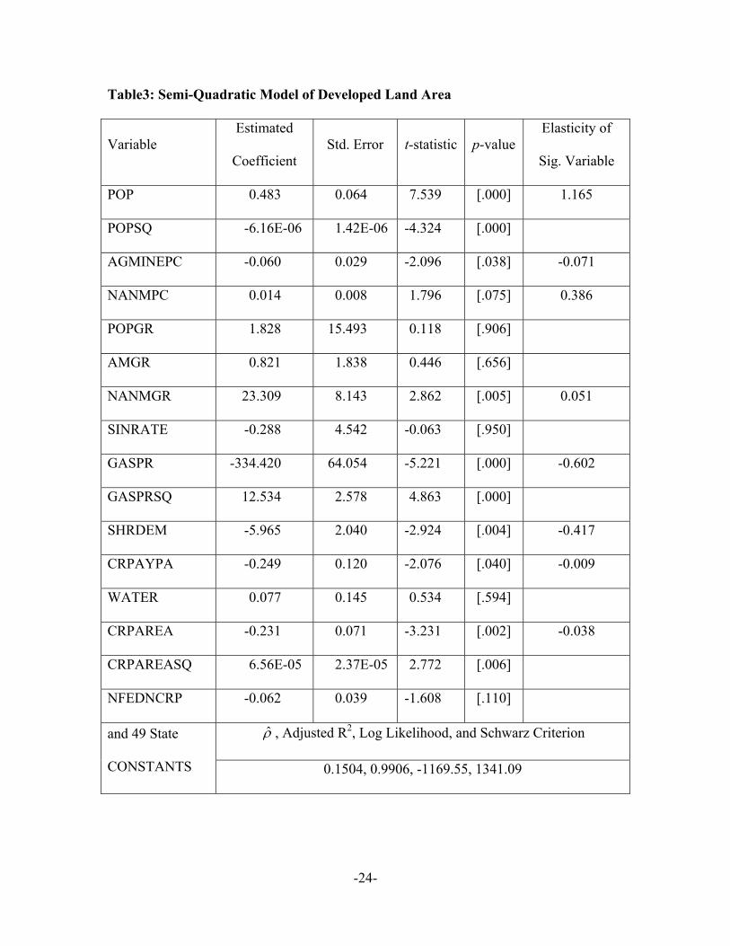
Table3: Semi-Quadratic Model of Developed Land Area
Variable Estimated
Coefficient Std. Error t-statistic p-value
Elasticity of
Sig. Variable
POP 0.483 0.064 7.539 [.000] 1.165
POPSQ -6.16E-06 1.42E-06 -4.324 [.000]
AGMINEPC -0.060 0.029 -2.096 [.038] -0.071
NANMPC 0.014 0.008 1.796 [.075] 0.386
POPGR 1.828 15.493 0.118 [.906]
AMGR 0.821 1.838 0.446 [.656]
NANMGR 23.309 8.143 2.862 [.005] 0.051
SINRATE -0.288 4.542 -0.063 [.950]
GASPR -334.420 64.054 -5.221 [.000] -0.602
GASPRSQ 12.534 2.578 4.863 [.000]
SHRDEM -5.965 2.040 -2.924 [.004] -0.417
CRPAYPA -0.249 0.120 -2.076 [.040] -0.009
WATER 0.077 0.145 0.534 [.594]
CRPAREA -0.231 0.071 -3.231 [.002] -0.038
CRPAREASQ 6.56E-05 2.37E-05 2.772 [.006]
NFEDNCRP -0.062 0.039 -1.608 [.110]
ρ̂ , Adjusted R2, Log Likelihood, and Schwarz Criterion and 49 State
CONSTANTS 0.1504, 0.9906, -1169.55, 1341.09
-24-