Systematic evaluation of soluble protein expression using a fluorescent unnatural amino acid reveals no reliable predictors of tolerability
Zachary M. Hostetler†, John J. Ferrie‡, Marc R. Bornstein†, Itthipol Sungwienwong‡,
E. James Petersson*,‡, Rahul M. Kohli**,†
†Department of Medicine, Department of Biochemistry and Biophysics, University of Pennsylvania,
Philadelphia, Pennsylvania 19104, United States ‡Department of Chemistry, University of Pennsylvania, Philadelphia, Pennsylvania 19104, United States
Corresponding Authors
*Email: [email protected].
**Email: [email protected].
ABSTRACT Improvements in genetic code expansion have made preparing proteins with diverse functional groups
almost routine. Nonetheless, unnatural amino acids (Uaas) pose theoretical burdens on protein solubility, and
determinants of position-specific tolerability to Uaas remain underexplored. To broadly examine associations,
we systematically assessed the effect of substituting the fluorescent Uaa, acridonylalanine, at more than fifty
chemically, evolutionarily, and structurally diverse residues in two bacterial proteins—LexA and RecA.
Surprisingly, properties that ostensibly contribute to Uaa tolerability—like conservation, hydrophobicity, or
accessibility—demonstrated no consistent correlations with resulting protein solubility. Instead, solubility closely
depended on the location of the substitution within the overall tertiary structure, suggesting that intrinsic
properties of protein domains, and not individual positions, are stronger determinants of Uaa tolerability.
Consequently, those who seek to install Uaas in new target proteins should consider broadening, rather than
narrowing, the types of residues screened for Uaa incorporation.
KEYWORDS Genetic code expansion, nonsense codon suppression, protein solubility, non-canonical amino acids, SOS
response
Technological advances in genetic code expansion have encouraged the design of proteins with a wide
range of reactive residues, post-translational modifications, photocaged groups, or intrinsic fluorophores.1–3
Nonsense codon suppression using orthogonal tRNA/aminoacyl-tRNA synthetase pairs enables direct
incorporation of chemically diverse unnatural amino acids (Uaas, also known as non-canonical amino acids) into
proteins in vivo. Many efforts have sought to boost the efficiency of Uaa incorporation, including evolving more
efficient aminoacyl-tRNA synthetases and recoding the E. coli genome to remove competing translational
release factors.4,5 Although these developments can improve total yields of modified proteins, factors governing
the position-dependent effects of Uaa substitution on protein solubility remain understudied.
Recent reports have demonstrated that the position of a Uaa can affect the level of total protein expressed,
both in cell-free and cell-based systems.6–10 Investigations of 20 positions in IFN-α and 33 positions in VSV
glycoprotein revealed varying total protein yields, from 0 to 95% of wildtype.11,12 Despite these observations,
explanations for position-dependent differences in total amounts of Uaa-containing proteins have been limited,
and no studies have explicitly addressed UAA incorporation versus the resulting protein solubility.
Unnatural amino acid mutagenesis could hypothetically operate under well-accepted principles that govern
the effects of natural amino acid mutation. For example, substitution of a nonpolar for a polar residue within the
hydrophobic core generally destabilizes proteins, whereas mutations on the solvent-exposed surface less
frequently affect solubility.13,14 Unsurprisingly, evolutionarily-conserved residues largely disfavor mutation.15–17
Substituting bulkier and more chemically-diverse Uaas into a protein can restrict function18 and therefore could
pose similar burdens on folding and solubility. Nevertheless, the applicability of principles of natural amino acid
mutagenesis to Uaa mutagenesis remains unknown.
Suggested guidelines or approaches for choosing Uaa-tolerant sites have been proposed. Some groups
favor residues with structural similarity to the Uaa.9 Others assert that candidate positions should be first
assessed for mutational tolerability with natural amino acids10 or that proteins should be thoroughly screened by
random incorporation of Uaas into protein-GFP fusions to reveal positions that label with high efficiency.19,20
Nonetheless, the feasibility of using position-specific properties to increase soluble protein expression remains
untested.
To address these open questions, we aimed to explore factors that impact Uaa incorporation and soluble
protein production. By employing an intrinsically fluorescent Uaa, acridonylalanine (Acd),6,21,22 we directly detect
labeled protein in cell lysate samples, overcoming the inability of past studies to measure levels of both total and
soluble expressed protein. Our systematic survey of more than fifty sites across two proteins reveals that while
incorporation efficiency is relatively similar, protein solubility, and by extension Uaa tolerability, varies widely
across different positions. However, most position-specific physicochemical, evolutionary, and structural
properties, some of which have been previously suggested to improve yield, were minimally predictive; instead,
solubility more strongly associated with the identity of the protein domain. After controlling for this domain effect,
we found that only a few factors, such as a tolerance for aromatic residues, moderately trended with protein
solubility. To our knowledge, this work currently represents the most systematic effort evaluating predictive
factors for producing soluble Uaa-containing proteins.
RESULTS AND DISCUSSION The bacterial protein LexA, a multi-domain repressor of the DNA damage response, has characteristics that
made it well-suited to this broader survey. Wild-type E. coli LexA is well-behaved in overexpression and has
previously tolerated selective unnatural amino acid (Uaa) incorporation.22 Additionally, the availability of protein
crystal structures and a multiple sequence alignment for LexA enabled retrieval of position-specific properties
from databases or servers that require these data as inputs (Table S1). For every position in LexA, we calculated
established metrics across different classes of properties: physicochemical, such as hydrophobicity;
evolutionary, such as conservation; and structural, such as solvent accessibility (Table 1). Using these metrics,
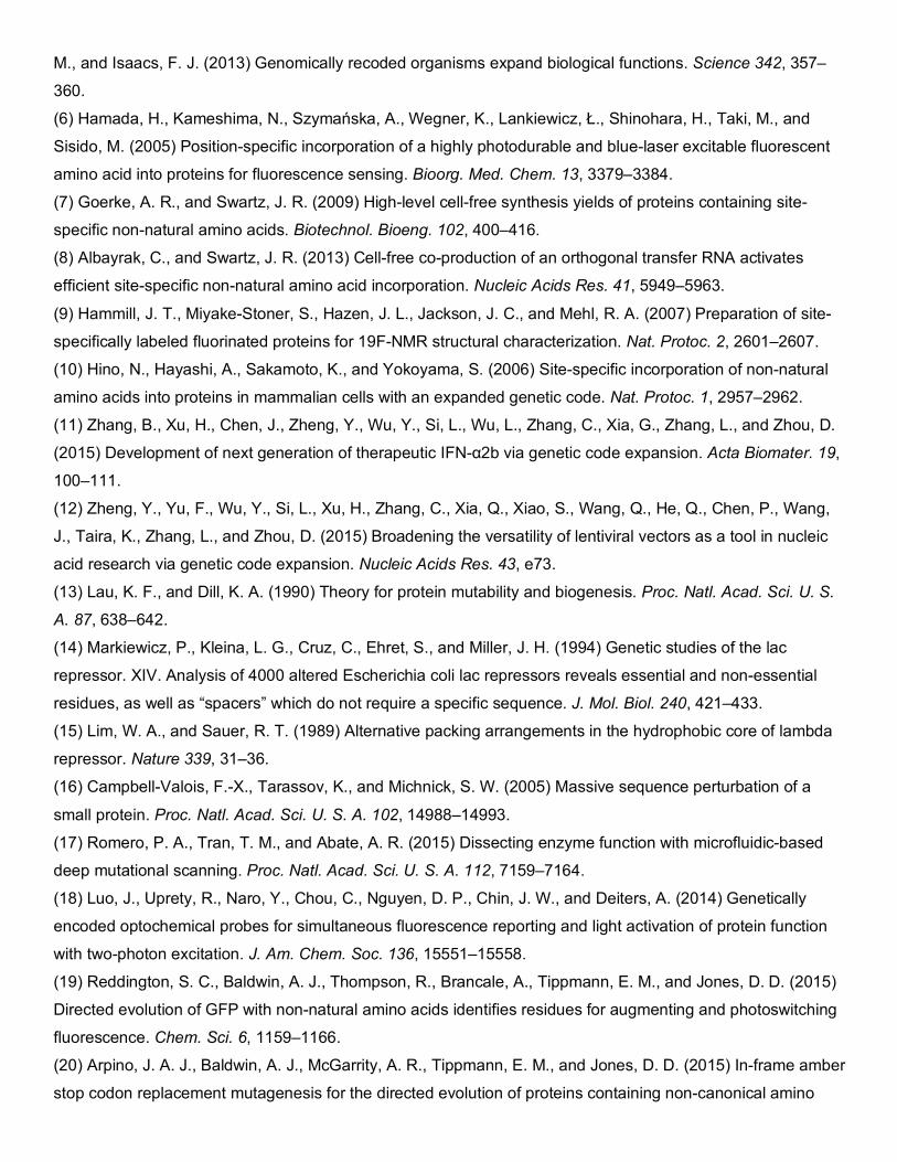
we selected 32 positions spanning both domains of LexA, deliberately avoiding known deleterious mutants as
well as the most conserved or hydrophobic positions (Figure 1a, Table S2). Our selected positions sample the
remaining metrics well (Figure 1b, Figure S1, and Figure S2), indicating that this series is well-positioned to
explore how aromatic, accessible, or poorly-conserved residues might differentially tolerate Uaa incorporation.
Historically, measuring Uaa incorporation efficiencies in vivo has overlooked protein solubility issues, while
labeling Uaa-containing proteins in vitro has suffered from incomplete sample recovery and detection. Crucially,
we chose to measure both total and soluble protein levels by using the fluorescent Uaa acridonylalanine (Acd,
Figure 1c), which already possesses an optimized tRNA/tRNA synthetase pair for in vivo incorporation.21,22 This
system offers several advantages. First, Acd incorporation occurs during protein overexpression without post-
translational labeling. Second, measurements of Acd fluorescence at the expected size on an SDS-PAGE gel
are directly proportional to levels of protein with successfully-incorporated Acd. Finally, gel-based detection of
Acd demonstrates a broad dynamic range, enabling us to detect quantitative differences in the expression of
Acd-containing LexA mutants (Figure S3).
Expression levels for a single protein can range widely due to experimental variability, making quantitative
comparison between different proteins difficult. To overcome this challenge, we overexpressed the 32 LexA
mutants in the presence of both Acd and the Acd-specific tRNA/tRNA synthetase using autoinduction media for
consistency in the timing and duration of protein production. Following overexpression, we measured
fluorescence intensity levels of Acd-containing LexA protein in both the whole cell lysate and soluble fraction
(Figure 1d). The use of purified Acd-containing LexA as a standard enabled quantitative and reproducible
comparisons of protein amounts across independent experiments (Figure S4).
Parallel overexpression of all 32 LexA mutants allowed us to investigate how amounts of total expressed
Acd-labeled LexA proteins differed (Table S3). A plot of logarithmically-transformed total protein amounts shows
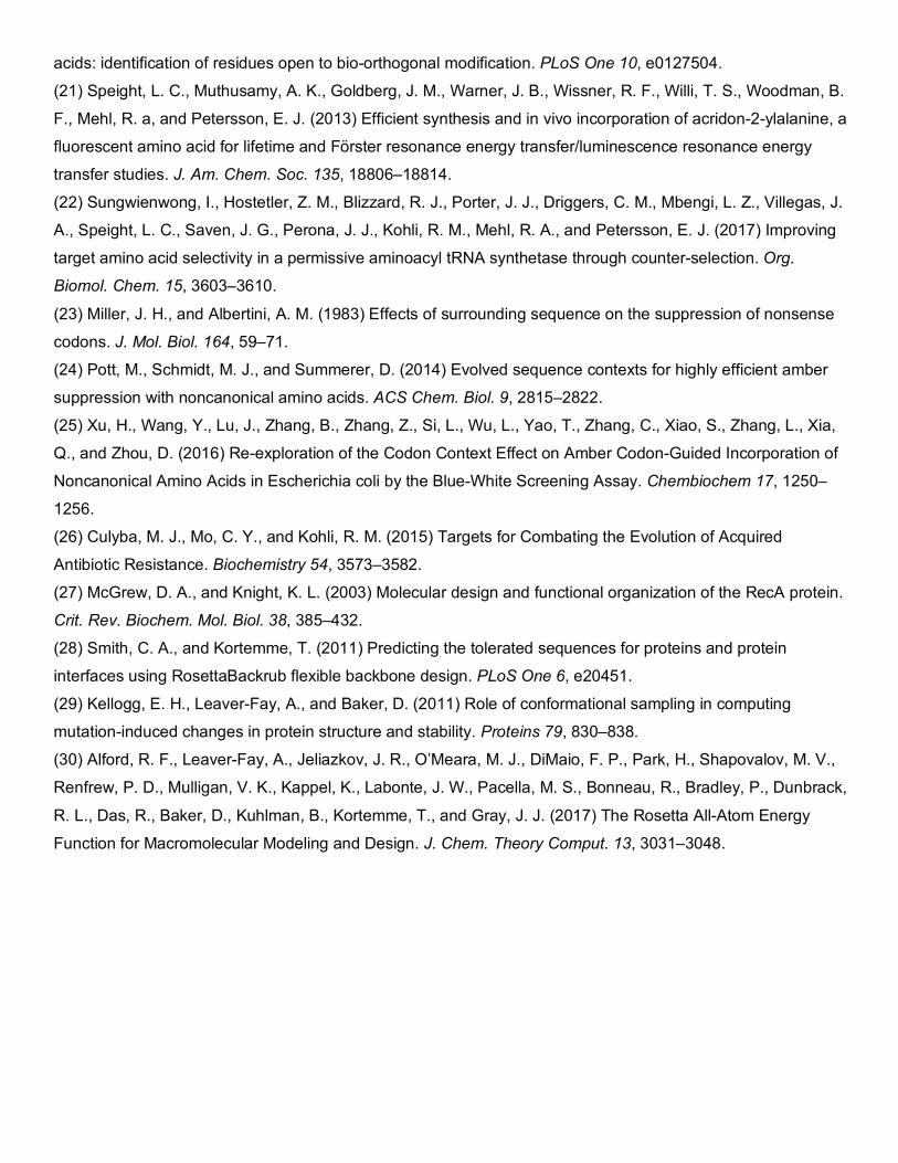
uniformly high protein expression (mean = 3.1) with minor variability (SD = 0.16) (Figure 2a). While past studies
have suggested that the identity of nucleotides surrounding the stop codon can impact nonsense codon
suppression efficiencies,23–25 we did not observe this relationship (Figure S5). Rather, the small 4.5-fold
difference between measurements of the lowest and highest-expressing samples suggests that changing the
position of Acd does not substantially alter Acd incorporation rates in vivo, and that incorporation is not a major
bottleneck with regards to solubility.
Recognizing the consistency in total levels of expressed protein, we next evaluated whether levels of soluble
protein differed. A distribution of logarithmically-transformed soluble protein amounts (Figure 2a) reveals more
variability (mean = 2.2, SD = 0.86). Measured soluble protein amounts ranged nearly 40-fold from the lowest
detectable measurements to the highest, a ten-fold increase over the range of total protein amounts. Because
both measurements are paired, we can isolate the position-dependent effect of Acd incorporation on solubility
by calculating the soluble fraction of total protein, which should exclude variability due to differences in total
protein production. The soluble fractions of Acd-labeled LexA mutants still vary considerably, from 0% to nearly
70% of total protein expressed (Figure 2b, Table S3). This result not only corroborates previous observations of
position-dependent effects on total protein expression,11,12 but it also establishes the heightened sensitivity of
protein solubility to Uaa incorporation.
Observing that the position of Acd can substantially impact protein solubility, we next asked which of the
properties that ostensibly affect Uaa tolerability might correlate with solubility. We fitted the soluble fraction as a
response variable to each property in individual linear regression models (Table S4 and Table S5). For almost
all of the properties we evaluated, the explained variability (adj. R2) was about 5% or less, indicating that if any
property-specific effect exists, it is insubstantial and likely below our ability to detect with a sample size of 32
(Figure S6 and Figure S7). We note that particular properties—such as accessibility, conservation, and
hydrophobicity—did not explain any substantial variation in our data, despite past suggestions that choosing
accessible, less-conserved, and chemically-similar residues may yield more soluble Uaa-containing protein
(Figure 2c).
Conspicuously, several highly-correlated properties each explained around 50% of the variability in our data,
including individual residue position (adj. R2 = 0.53), secondary structure (adj. R2 = 0.45), and overall protein
domain (adj. R2 = 0.53) (Figure 2d and Figure 2e). Specifically, we obtained more soluble protein when Acd was
incorporated within the first 74 residues of LexA, which includes all three of the α-helices that comprise the N-
terminal domain. By contrast, Acd incorporation within the β-sheets of the C-terminal domain resulted in much
lower proportions of soluble protein. The nearly uniform secondary structure composition of each domain limited
our ability to interpret whether Acd tolerability is due to local secondary structure effects or global protein domain
stabilities.
Excluding the effect that secondary or tertiary structure has on protein solubility could reveal minor trends
obscured in the overall dataset. To address this possibility, in individual linear regression models, we fitted each
property along with protein domain as explanatory factors for the soluble fraction (Table S6 and Table S7). By
controlling for domain, we could detect a minor correlation between the soluble fraction and the evolutionary
tolerance of any given position to an aromatic residue (Figure 2f). However, remaining factors—including notable
ones such as conservation, hydrophobicity, and accessibility—either did not explain any substantial variation in
the data or demonstrated inconsistent trends between domains (Figure 2c). Consequently, our extended LexA
analysis reaffirmed that the tolerability of a protein domain to Acd—or possibly the tolerability of a secondary
structure type—overwhelmingly determines soluble protein expression.
Studying Acd incorporation in a distinct protein scaffold with mixed α/β character could help dissect the similar
effects we observed from the highly-correlated domain and secondary structure factors with LexA. Thus, we
extended our survey to RecA, a bacterial ATPase that binds LexA to suppress its repressor function.26 We
selected positions in E. coli RecA that satisfied one or more criteria: high accessibility, low conservation, few
inter-residue contacts, or prior functional tolerance to mutation (Figure 3a).27 After expressing these mutants with
Acd and measuring protein amounts, we again observed greater variability in logarithmically-transformed soluble
protein levels (mean = 3.42, SD = 0.40) compared to total protein levels (mean = 3.72, SD = 0.17) (Figure 3b,
Figure 3c, Table S8). Similar to LexA, most properties examined did not explain much variation in the fractions
of soluble protein (Figure 3d), with the exception that solubility modestly trended with domain type and tolerance
to aromatics (Table S9). However, unlike in LexA, no clear relationship existed between protein solubility and
type of secondary structure (Figure 3e), a result consistent with a more limited prior survey of GFP.8 This survey
in RecA bolsters a model in which the intrinsic Uaa tolerability of a protein domain remains the key obstacle for
the production of soluble protein.
Searching for easily-determined properties that correlate with Acd tolerability may have eliminated from
consideration more complicated properties with higher predictive ability. Additionally, linear regression modeling
may have over-simplified the inter-dependence of certain properties and protein solubility. Previously, Rosetta
modeling has predicted the ΔΔG associated with a particular mutation and identified tolerated mutations within
a protein.28–30 Speculating that Rosetta modeling could recapitulate our experimental results, we used the
Rosetta Modeling Suite to simulate the resulting energy associated with Acd incorporation in LexA or RecA.
However, we observed no significant correlations between simulated energies and soluble fractions of LexA or
RecA (Figure S8 and Figure S9). Incidentally, we noted that nearly all high-energy positions in LexA
experimentally yielded insoluble protein and may therefore have been useful in filtering out those positions;
however, we did not observe a similar energy threshold effect for RecA. Accordingly, further refinement towards
predicting Uaa incorporation using Rosetta is required in order to recapitulate experimental data and exclude
higher-energy and lower-solubility mutants.
CONCLUSION The expression of soluble protein is a major bottleneck for the study of protein function. Here, we leveraged
the fluorescence of Acd to study how protein solubility is impacted by Uaa mutagenesis. In two bacterial proteins,
we demonstrated the dramatic impact that Uaa position has on protein solubility. Surprisingly, a number of amino
acid properties that purportedly contribute to Uaa tolerability—including low evolutionary conservation, similar
hydrophobic character, or high surface accessibility—were unreliable predictors of protein solubility. Instead,
these inconsistent relationships suggest that consideration of specific amino acid features for successful Uaa
mutagenesis is less critical than previously thought. Rather, we speculate that the Uaa tolerability of a protein
domain may matter more. Our results also emphasize a continued need to explore, through theory and
experiment, the steric and chemical burdens different Uaas pose to the expression of soluble protein. In the
absence of reliable predictors or refined simulation algorithms for Uaa tolerability, a chemical biologist pursuing
Uaa incorporation in a new protein, as of now, should broaden rather than narrow the types of residues screened
for Uaa tolerability when possible.
ASSOCIATED CONTENT Supporting Information
Supporting Information Available: The following material is available free of charge via the internet.
Experimental methods, supplemental figures and tables, and associated references.
AUTHOR INFORMATION ORCID Zachary M. Hostetler: 0000-0002-2830-8870
John J. Ferrie: 0000-0001-7934-7266
E. James Petersson: 0000-0003-3854-9210
Rahul M. Kohli: 0000-0002-7689-5678
Author Contributions Z.M.H., J.J.F., M.R.B., I.S., E.J.P, and R.M.K. designed the experiments. Z.M.H performed all the experiments
with assistance from M.R.B. J.J.F. performed the Rosetta simulations. I.S. synthesized Acd. Z.M.H. and J.J.F.
performed the data analysis with input from all authors. Z.M.H., E.J.P., and R.M.K. wrote the manuscript with
input from all authors.
Notes The authors declare no competing financial interest.
ACKNOWLEDGMENTS We thank members of the Kohli and Petersson laboratories for general advice, and we are grateful to E. Schutsky
for input in preparing the manuscript. This work was supported by the National Institutes of Health (R01-
GM127593 to R.M.K. and E.J.P.) and the National Science Foundation (NSF, CHE-1708759 to E.J.P.). Z.M.H.
was supported by the NIH Chemistry Biology Interface Training Program (T32-GM071399). J.J.F. was supported
by the NSF Graduate Research Fellowship Program (DGE-1321851). I.S. was supported by the Royal Thai
Foundation.
REFERENCES (1) Young, T. S., and Schultz, P. G. (2010) Beyond the Canonical 20 Amino Acids: Expanding the Genetic
Lexicon. J. Biol. Chem. 285, 11039–11044.
(2) Neumann-Staubitz, P., and Neumann, H. (2016) The use of unnatural amino acids to study and engineer
protein function. Curr. Opin. Struct. Biol. 38, 119–128.
(3) Xiao, H., and Schultz, P. G. (2016) At the Interface of Chemical and Biological Synthesis: An Expanded
Genetic Code. Cold Spring Harb. Perspect. Biol. 8, a023945.
(4) Chatterjee, A., Sun, S. B., Furman, J. L., Xiao, H., and Schultz, P. G. (2013) A Versatile Platform for Single-
and Multiple-Unnatural Amino Acid Mutagenesis in Escherichia coli. Biochemistry 52, 1828–1837.
(5) Lajoie, M. J., Rovner, A. J., Goodman, D. B., Aerni, H.-R., Haimovich, A. D., Kuznetsov, G., Mercer, J. a,
Wang, H. H., Carr, P. a, Mosberg, J. a, Rohland, N., Schultz, P. G., Jacobson, J. M., Rinehart, J., Church, G.
M., and Isaacs, F. J. (2013) Genomically recoded organisms expand biological functions. Science 342, 357–
360.
(6) Hamada, H., Kameshima, N., Szymańska, A., Wegner, K., Lankiewicz, Ł., Shinohara, H., Taki, M., and
Sisido, M. (2005) Position-specific incorporation of a highly photodurable and blue-laser excitable fluorescent
amino acid into proteins for fluorescence sensing. Bioorg. Med. Chem. 13, 3379–3384.
(7) Goerke, A. R., and Swartz, J. R. (2009) High-level cell-free synthesis yields of proteins containing site-
specific non-natural amino acids. Biotechnol. Bioeng. 102, 400–416.
(8) Albayrak, C., and Swartz, J. R. (2013) Cell-free co-production of an orthogonal transfer RNA activates
efficient site-specific non-natural amino acid incorporation. Nucleic Acids Res. 41, 5949–5963.
(9) Hammill, J. T., Miyake-Stoner, S., Hazen, J. L., Jackson, J. C., and Mehl, R. A. (2007) Preparation of site-
specifically labeled fluorinated proteins for 19F-NMR structural characterization. Nat. Protoc. 2, 2601–2607.
(10) Hino, N., Hayashi, A., Sakamoto, K., and Yokoyama, S. (2006) Site-specific incorporation of non-natural
amino acids into proteins in mammalian cells with an expanded genetic code. Nat. Protoc. 1, 2957–2962.
(11) Zhang, B., Xu, H., Chen, J., Zheng, Y., Wu, Y., Si, L., Wu, L., Zhang, C., Xia, G., Zhang, L., and Zhou, D.
(2015) Development of next generation of therapeutic IFN-α2b via genetic code expansion. Acta Biomater. 19,
100–111.
(12) Zheng, Y., Yu, F., Wu, Y., Si, L., Xu, H., Zhang, C., Xia, Q., Xiao, S., Wang, Q., He, Q., Chen, P., Wang,
J., Taira, K., Zhang, L., and Zhou, D. (2015) Broadening the versatility of lentiviral vectors as a tool in nucleic
acid research via genetic code expansion. Nucleic Acids Res. 43, e73.
(13) Lau, K. F., and Dill, K. A. (1990) Theory for protein mutability and biogenesis. Proc. Natl. Acad. Sci. U. S.
A. 87, 638–642.
(14) Markiewicz, P., Kleina, L. G., Cruz, C., Ehret, S., and Miller, J. H. (1994) Genetic studies of the lac
repressor. XIV. Analysis of 4000 altered Escherichia coli lac repressors reveals essential and non-essential
residues, as well as “spacers” which do not require a specific sequence. J. Mol. Biol. 240, 421–433.
(15) Lim, W. A., and Sauer, R. T. (1989) Alternative packing arrangements in the hydrophobic core of lambda
repressor. Nature 339, 31–36.
(16) Campbell-Valois, F.-X., Tarassov, K., and Michnick, S. W. (2005) Massive sequence perturbation of a
small protein. Proc. Natl. Acad. Sci. U. S. A. 102, 14988–14993.
(17) Romero, P. A., Tran, T. M., and Abate, A. R. (2015) Dissecting enzyme function with microfluidic-based
deep mutational scanning. Proc. Natl. Acad. Sci. U. S. A. 112, 7159–7164.
(18) Luo, J., Uprety, R., Naro, Y., Chou, C., Nguyen, D. P., Chin, J. W., and Deiters, A. (2014) Genetically
encoded optochemical probes for simultaneous fluorescence reporting and light activation of protein function
with two-photon excitation. J. Am. Chem. Soc. 136, 15551–15558.
(19) Reddington, S. C., Baldwin, A. J., Thompson, R., Brancale, A., Tippmann, E. M., and Jones, D. D. (2015)
Directed evolution of GFP with non-natural amino acids identifies residues for augmenting and photoswitching
fluorescence. Chem. Sci. 6, 1159–1166.
(20) Arpino, J. A. J., Baldwin, A. J., McGarrity, A. R., Tippmann, E. M., and Jones, D. D. (2015) In-frame amber
stop codon replacement mutagenesis for the directed evolution of proteins containing non-canonical amino
acids: identification of residues open to bio-orthogonal modification. PLoS One 10, e0127504.
(21) Speight, L. C., Muthusamy, A. K., Goldberg, J. M., Warner, J. B., Wissner, R. F., Willi, T. S., Woodman, B.
F., Mehl, R. a, and Petersson, E. J. (2013) Efficient synthesis and in vivo incorporation of acridon-2-ylalanine, a
fluorescent amino acid for lifetime and Förster resonance energy transfer/luminescence resonance energy
transfer studies. J. Am. Chem. Soc. 135, 18806–18814.
(22) Sungwienwong, I., Hostetler, Z. M., Blizzard, R. J., Porter, J. J., Driggers, C. M., Mbengi, L. Z., Villegas, J.
A., Speight, L. C., Saven, J. G., Perona, J. J., Kohli, R. M., Mehl, R. A., and Petersson, E. J. (2017) Improving
target amino acid selectivity in a permissive aminoacyl tRNA synthetase through counter-selection. Org.
Biomol. Chem. 15, 3603–3610.
(23) Miller, J. H., and Albertini, A. M. (1983) Effects of surrounding sequence on the suppression of nonsense
codons. J. Mol. Biol. 164, 59–71.
(24) Pott, M., Schmidt, M. J., and Summerer, D. (2014) Evolved sequence contexts for highly efficient amber
suppression with noncanonical amino acids. ACS Chem. Biol. 9, 2815–2822.
(25) Xu, H., Wang, Y., Lu, J., Zhang, B., Zhang, Z., Si, L., Wu, L., Yao, T., Zhang, C., Xiao, S., Zhang, L., Xia,
Q., and Zhou, D. (2016) Re-exploration of the Codon Context Effect on Amber Codon-Guided Incorporation of
Noncanonical Amino Acids in Escherichia coli by the Blue-White Screening Assay. Chembiochem 17, 1250–
1256.
(26) Culyba, M. J., Mo, C. Y., and Kohli, R. M. (2015) Targets for Combating the Evolution of Acquired
Antibiotic Resistance. Biochemistry 54, 3573–3582.
(27) McGrew, D. A., and Knight, K. L. (2003) Molecular design and functional organization of the RecA protein.
Crit. Rev. Biochem. Mol. Biol. 38, 385–432.
(28) Smith, C. A., and Kortemme, T. (2011) Predicting the tolerated sequences for proteins and protein
interfaces using RosettaBackrub flexible backbone design. PLoS One 6, e20451.
(29) Kellogg, E. H., Leaver-Fay, A., and Baker, D. (2011) Role of conformational sampling in computing
mutation-induced changes in protein structure and stability. Proteins 79, 830–838.
(30) Alford, R. F., Leaver-Fay, A., Jeliazkov, J. R., O’Meara, M. J., DiMaio, F. P., Park, H., Shapovalov, M. V.,
Renfrew, P. D., Mulligan, V. K., Kappel, K., Labonte, J. W., Pacella, M. S., Bonneau, R., Bradley, P., Dunbrack,
R. L., Das, R., Baker, D., Kuhlman, B., Kortemme, T., and Gray, J. J. (2017) The Rosetta All-Atom Energy
Function for Macromolecular Modeling and Design. J. Chem. Theory Comput. 13, 3031–3048.
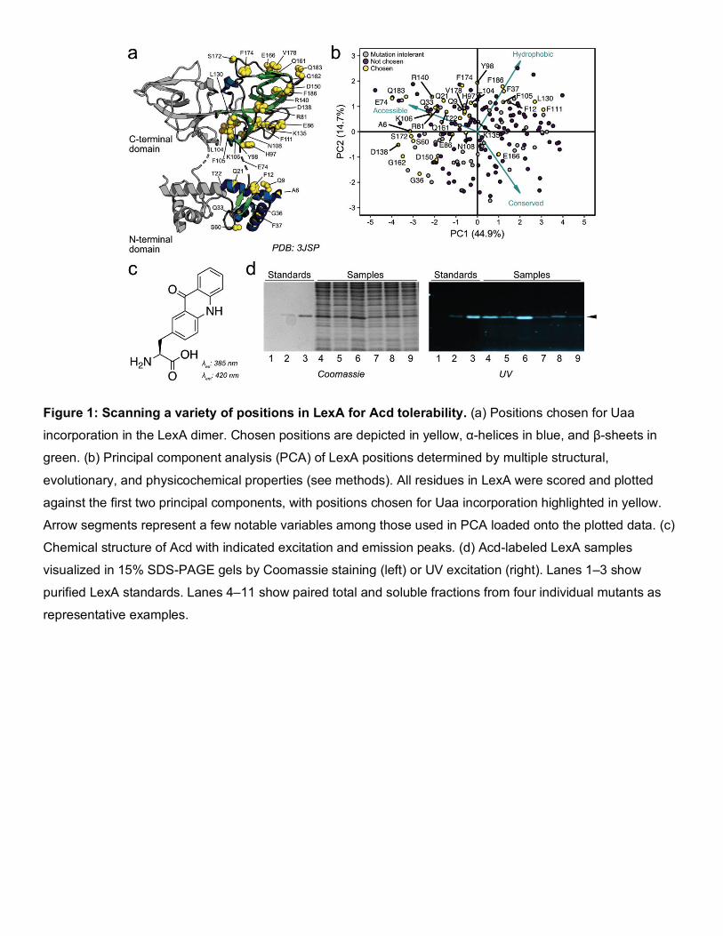
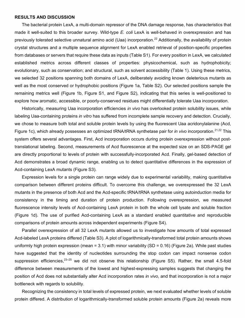
Figure 1: Scanning a variety of positions in LexA for Acd tolerability. (a) Positions chosen for Uaa
incorporation in the LexA dimer. Chosen positions are depicted in yellow, α-helices in blue, and β-sheets in
green. (b) Principal component analysis (PCA) of LexA positions determined by multiple structural,
evolutionary, and physicochemical properties (see methods). All residues in LexA were scored and plotted
against the first two principal components, with positions chosen for Uaa incorporation highlighted in yellow.
Arrow segments represent a few notable variables among those used in PCA loaded onto the plotted data. (c)
Chemical structure of Acd with indicated excitation and emission peaks. (d) Acd-labeled LexA samples
visualized in 15% SDS-PAGE gels by Coomassie staining (left) or UV excitation (right). Lanes 1–3 show
purified LexA standards. Lanes 4–11 show paired total and soluble fractions from four individual mutants as
representative examples.
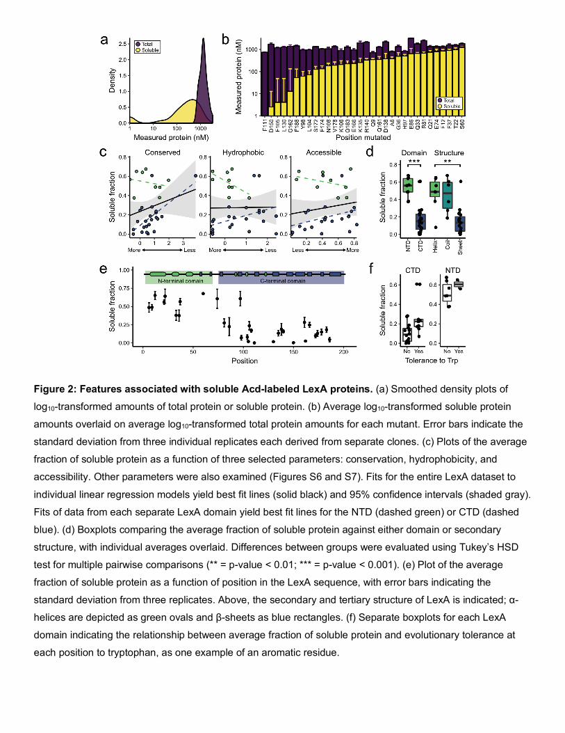
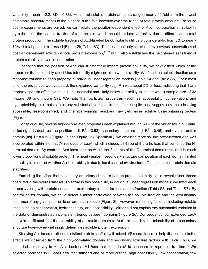
Figure 2: Features associated with soluble Acd-labeled LexA proteins. (a) Smoothed density plots of
log10-transformed amounts of total protein or soluble protein. (b) Average log10-transformed soluble protein
amounts overlaid on average log10-transformed total protein amounts for each mutant. Error bars indicate the
standard deviation from three individual replicates each derived from separate clones. (c) Plots of the average
fraction of soluble protein as a function of three selected parameters: conservation, hydrophobicity, and
accessibility. Other parameters were also examined (Figures S6 and S7). Fits for the entire LexA dataset to
individual linear regression models yield best fit lines (solid black) and 95% confidence intervals (shaded gray).
Fits of data from each separate LexA domain yield best fit lines for the NTD (dashed green) or CTD (dashed
blue). (d) Boxplots comparing the average fraction of soluble protein against either domain or secondary
structure, with individual averages overlaid. Differences between groups were evaluated using Tukey’s HSD
test for multiple pairwise comparisons (** = p-value < 0.01; *** = p-value < 0.001). (e) Plot of the average
fraction of soluble protein as a function of position in the LexA sequence, with error bars indicating the
standard deviation from three replicates. Above, the secondary and tertiary structure of LexA is indicated; α-
helices are depicted as green ovals and β-sheets as blue rectangles. (f) Separate boxplots for each LexA
domain indicating the relationship between average fraction of soluble protein and evolutionary tolerance at
each position to tryptophan, as one example of an aromatic residue.
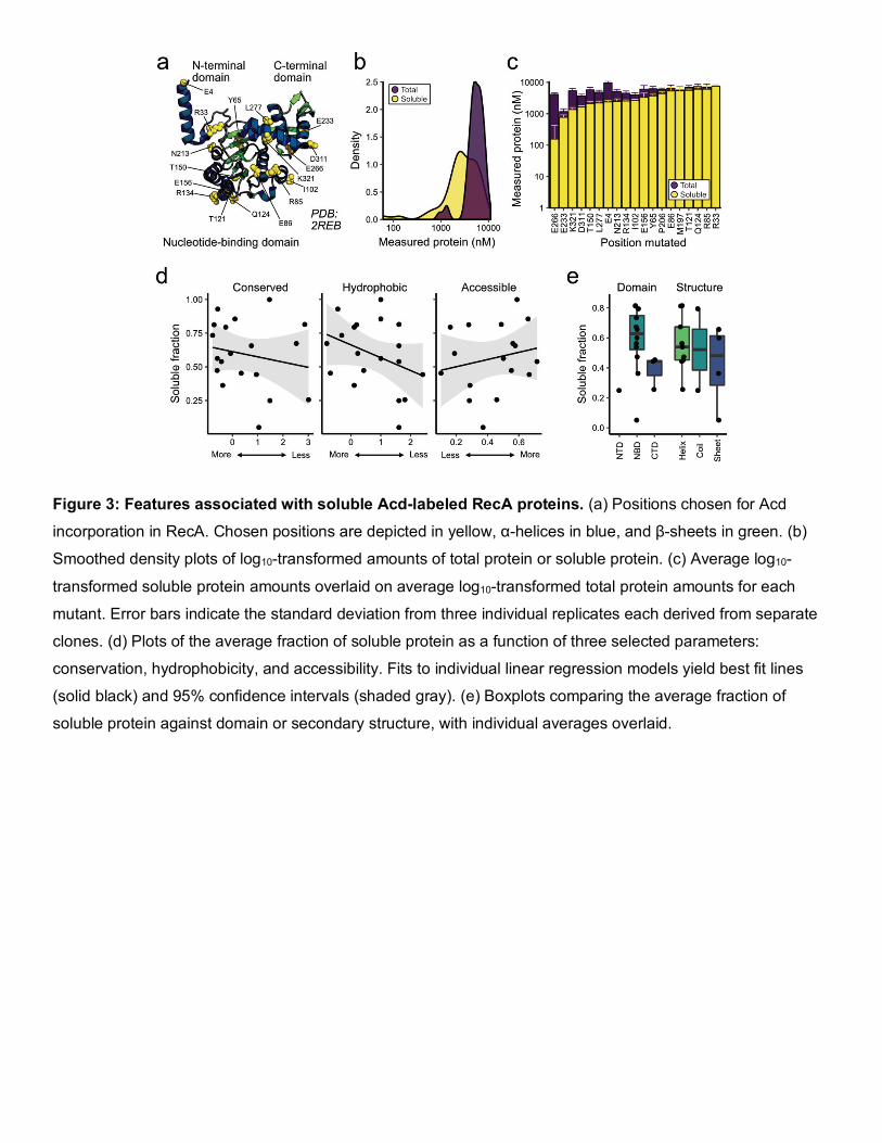
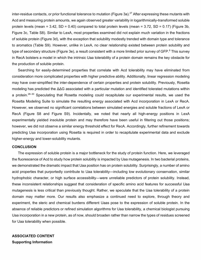
Figure 3: Features associated with soluble Acd-labeled RecA proteins. (a) Positions chosen for Acd
incorporation in RecA. Chosen positions are depicted in yellow, α-helices in blue, and β-sheets in green. (b)
Smoothed density plots of log10-transformed amounts of total protein or soluble protein. (c) Average log10-
transformed soluble protein amounts overlaid on average log10-transformed total protein amounts for each
mutant. Error bars indicate the standard deviation from three individual replicates each derived from separate
clones. (d) Plots of the average fraction of soluble protein as a function of three selected parameters:
conservation, hydrophobicity, and accessibility. Fits to individual linear regression models yield best fit lines
(solid black) and 95% confidence intervals (shaded gray). (e) Boxplots comparing the average fraction of
soluble protein against domain or secondary structure, with individual averages overlaid.
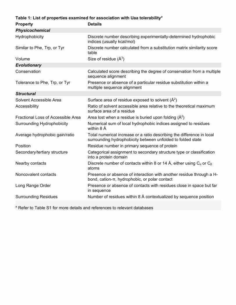
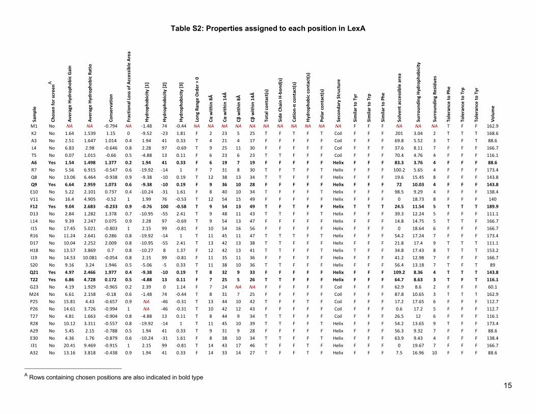
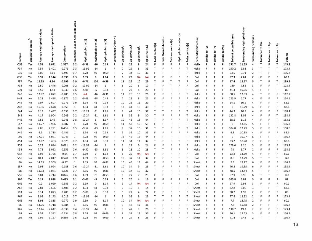
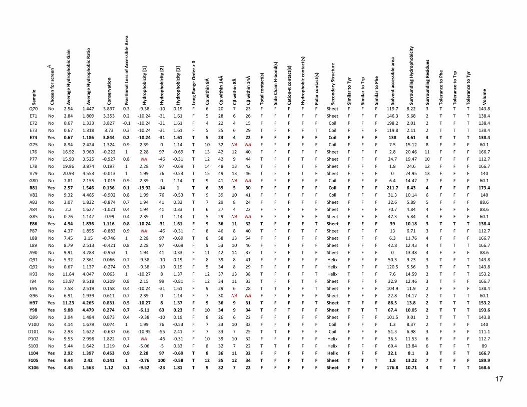
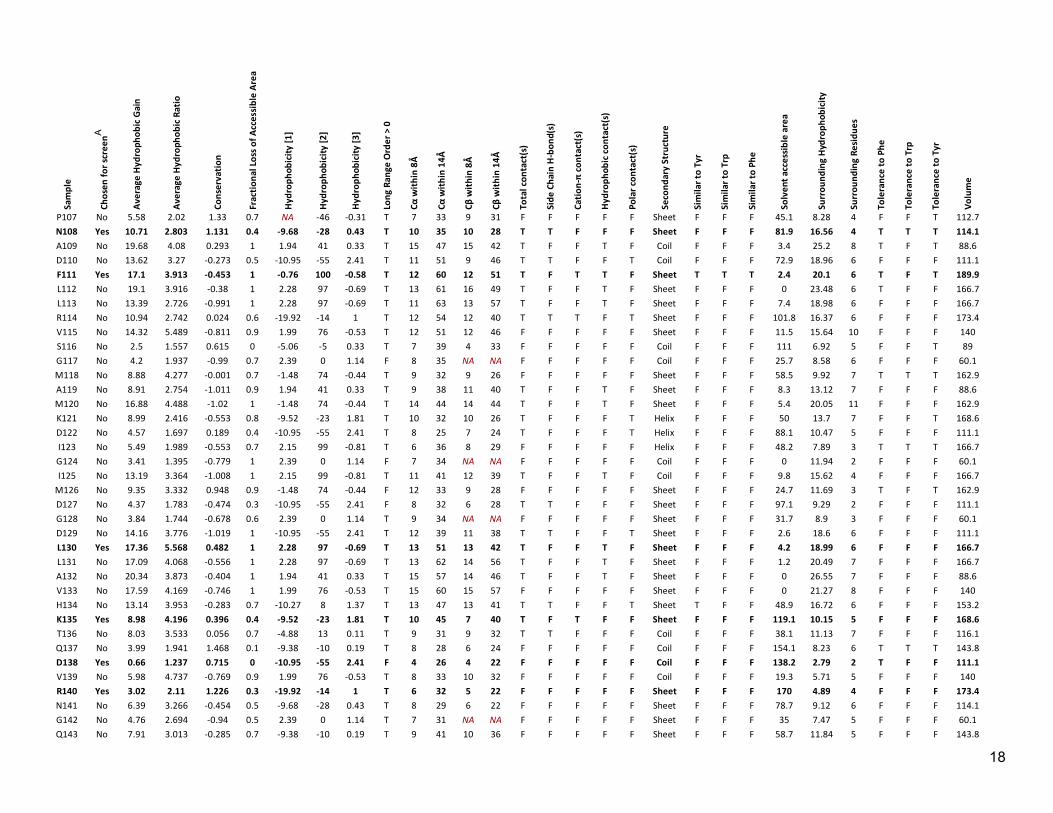
Table 1: List of properties examined for association with Uaa tolerabilitya
Property Details Physicochemical Hydrophobicity Discrete number describing experimentally-determined hydrophobic
indices (usually kcal/mol) Similar to Phe, Trp, or Tyr Discrete number calculated from a substitution matrix similarity score
table Volume Size of residue (Å3) Evolutionary Conservation Calculated score describing the degree of conservation from a multiple
sequence alignment Tolerance to Phe, Trp, or Tyr Presence or absence of a particular residue substitution within a
multiple sequence alignment Structural Solvent Accessible Area Surface area of residue exposed to solvent (Å2) Accessibility Ratio of solvent accessible area relative to the theoretical maximum
surface area of a residue Fractional Loss of Accessible Area Area lost when a residue is buried upon folding (Å2) Surrounding Hydrophobicity Numerical sum of local hydrophobic indices assigned to residues
within 8 Å Average hydrophobic gain/ratio Total numerical increase or a ratio describing the difference in local
surrounding hydrophobicity between unfolded to folded state Position Residue number in primary sequence of protein Secondary/tertiary structure Categorical assignment to secondary structure type or classification
into a protein domain Nearby contacts Discrete number of contacts within 8 or 14 Å, either using Cα or Cβ
atoms Noncovalent contacts Presence or absence of interaction with another residue through a H-
bond, cation-π, hydrophobic, or polar contact Long Range Order Presence or absence of contacts with residues close in space but far
in sequence Surrounding Residues Number of residues within 8 Å contextualized by sequence position a Refer to Table S1 for more details and references to relevant databases
Systematic evaluation of soluble protein expression using a fluorescent unnatural amino acid reveals
no reliable predictors of tolerability
Zachary M. Hostetler†, John J. Ferrie‡, Marc R. Bornstein†, Itthipol Sungwienwong‡,
E. James Petersson‡, Rahul M. Kohli†
†Department of Medicine, Department of Biochemistry and Biophysics, University of Pennsylvania,
Philadelphia, Pennsylvania 19104, United States ‡Department of Chemistry, University of Pennsylvania, Philadelphia, Pennsylvania 19104, United States
Experimental Methods Amber stop codon mutagenesis in LexA and RecA overexpression plasmids .......................................... 2 Parallel overexpression of LexA or RecA mutants ....................................................................................... 2 Cell lysis and soluble protein fractionation ................................................................................................... 2 Determination of properties from sequence and structure files .................................................................. 2 Specific detection of Acd fluorescence ......................................................................................................... 3 Simulation of Acd incorporation into LexA or RecA with Rosetta ............................................................... 3 Exploring amino acid properties and levels of Acd-labeled proteins .......................................................... 4 Supplemental Figures Figure S1: Sampling of numerical properties by chosen positions in LexA ............................................... 5 Figure S2: Sampling of categorical properties by chosen positions in LexA. ............................................ 6 Figure S3: Dynamic range determination from purified LexA standards .................................................... 7 Figure S4: Reproducibility of experimental approach .................................................................................. 8 Figure S5: Effect of neighboring nucleotides on amber stop codon suppression efficiency.................... 9 Figure S6: Effect of individual numerical properties on LexA solubility ................................................... 10 Figure S7: Effect of individual categorical properties on LexA solubility ................................................. 11 Figure S8: Predicting protein solubility through simulation of Acd incorporation in LexA ..................... 12 Figure S9: Predicting protein solubility through simulation of Acd incorporation in RecA .................... 13
Supplemental Tables Table S1: Expanded list of properties examined for association with Uaa tolerability ............................ 14 Table S2: Properties assigned to each position in LexA ............................................................................ 15 Table S3: Measured total and soluble amounts of fluorescent LexA ........................................................ 21 Table S4: Summary statistics of linear regression models for categorical properties with LexA ........... 22 Table S5: Summary statistics of linear regression models for numerical properties with LexA ............. 23 Table S6: Categorical property coefficients for two-factor linear regression models with LexA ............ 24 Table S7: Numerical property coefficients for two-factor linear regression models with LexA .............. 25 Table S8: Measured total and soluble amounts of fluorescent RecA ........................................................ 26 Table S9: Summary statistics of linear regression models with RecA ...................................................... 27
2
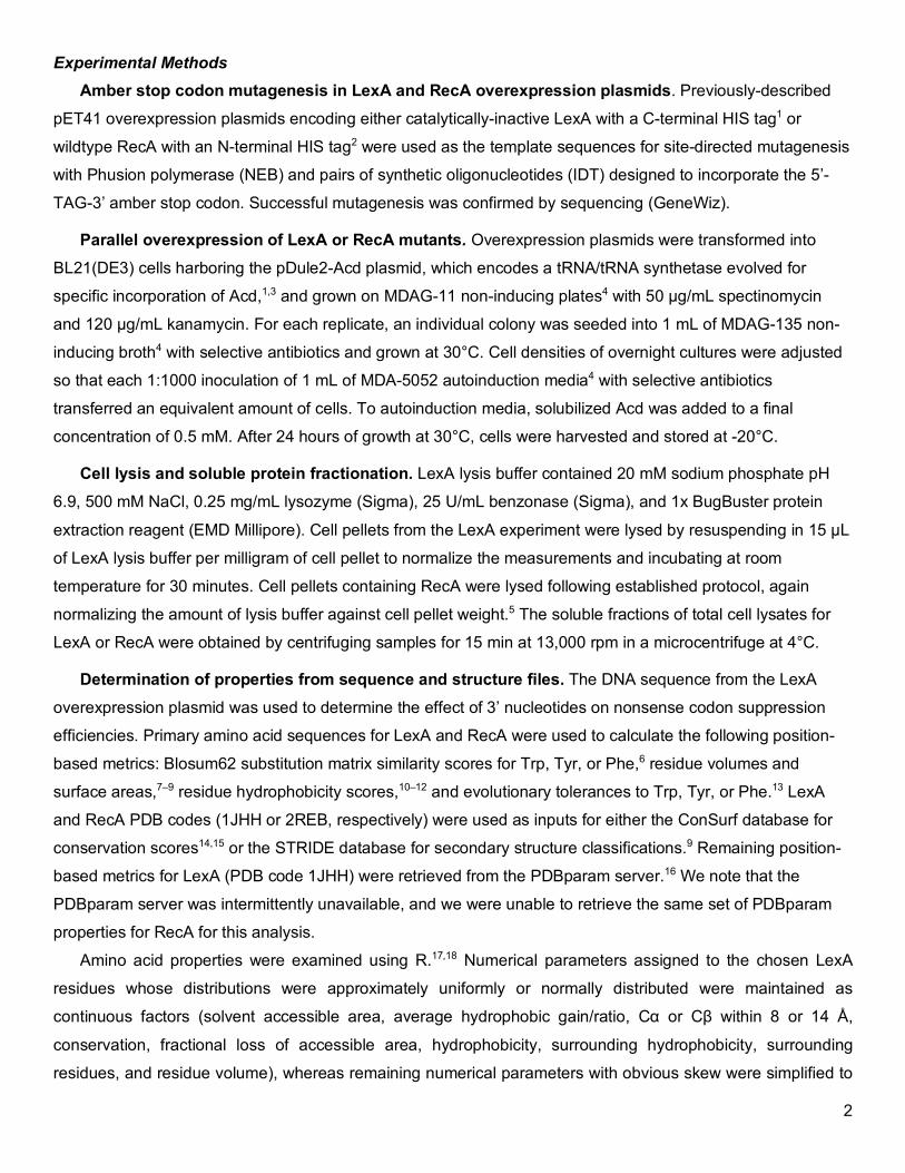
Experimental Methods Amber stop codon mutagenesis in LexA and RecA overexpression plasmids. Previously-described
pET41 overexpression plasmids encoding either catalytically-inactive LexA with a C-terminal HIS tag1 or
wildtype RecA with an N-terminal HIS tag2 were used as the template sequences for site-directed mutagenesis
with Phusion polymerase (NEB) and pairs of synthetic oligonucleotides (IDT) designed to incorporate the 5’-
TAG-3’ amber stop codon. Successful mutagenesis was confirmed by sequencing (GeneWiz).
Parallel overexpression of LexA or RecA mutants. Overexpression plasmids were transformed into
BL21(DE3) cells harboring the pDule2-Acd plasmid, which encodes a tRNA/tRNA synthetase evolved for
specific incorporation of Acd,1,3 and grown on MDAG-11 non-inducing plates4 with 50 μg/mL spectinomycin
and 120 μg/mL kanamycin. For each replicate, an individual colony was seeded into 1 mL of MDAG-135 non-
inducing broth4 with selective antibiotics and grown at 30°C. Cell densities of overnight cultures were adjusted
so that each 1:1000 inoculation of 1 mL of MDA-5052 autoinduction media4 with selective antibiotics
transferred an equivalent amount of cells. To autoinduction media, solubilized Acd was added to a final
concentration of 0.5 mM. After 24 hours of growth at 30°C, cells were harvested and stored at -20°C.
Cell lysis and soluble protein fractionation. LexA lysis buffer contained 20 mM sodium phosphate pH
6.9, 500 mM NaCl, 0.25 mg/mL lysozyme (Sigma), 25 U/mL benzonase (Sigma), and 1x BugBuster protein
extraction reagent (EMD Millipore). Cell pellets from the LexA experiment were lysed by resuspending in 15 µL
of LexA lysis buffer per milligram of cell pellet to normalize the measurements and incubating at room
temperature for 30 minutes. Cell pellets containing RecA were lysed following established protocol, again
normalizing the amount of lysis buffer against cell pellet weight.5 The soluble fractions of total cell lysates for
LexA or RecA were obtained by centrifuging samples for 15 min at 13,000 rpm in a microcentrifuge at 4°C.
Determination of properties from sequence and structure files. The DNA sequence from the LexA
overexpression plasmid was used to determine the effect of 3’ nucleotides on nonsense codon suppression
efficiencies. Primary amino acid sequences for LexA and RecA were used to calculate the following position-
based metrics: Blosum62 substitution matrix similarity scores for Trp, Tyr, or Phe,6 residue volumes and
surface areas,7–9 residue hydrophobicity scores,10–12 and evolutionary tolerances to Trp, Tyr, or Phe.13 LexA
and RecA PDB codes (1JHH or 2REB, respectively) were used as inputs for either the ConSurf database for
conservation scores14,15 or the STRIDE database for secondary structure classifications.9 Remaining position-
based metrics for LexA (PDB code 1JHH) were retrieved from the PDBparam server.16 We note that the
PDBparam server was intermittently unavailable, and we were unable to retrieve the same set of PDBparam
properties for RecA for this analysis.
Amino acid properties were examined using R.17,18 Numerical parameters assigned to the chosen LexA
residues whose distributions were approximately uniformly or normally distributed were maintained as
continuous factors (solvent accessible area, average hydrophobic gain/ratio, Cα or Cβ within 8 or 14 Å,
conservation, fractional loss of accessible area, hydrophobicity, surrounding hydrophobicity, surrounding
residues, and residue volume), whereas remaining numerical parameters with obvious skew were simplified to
3
categorical factors. The degree to which each property was sampled by the chosen positions in LexA was
assessed by plotting individual histograms or bar charts (Figure S1 and Figure S2). A more rigorous assessment
of the variability of the chosen positions was accomplished through a principal component analysis. From the
above continuous factors, highly-correlated parameters were dropped; the remaining continuous factors (solvent
accessible area, average hydrophobic ratio, alpha carbons within 14 Å, conservation, hydrophobicity,
surrounding hydrophobic residues, surrounding residues, and residue volume) were used to generate principal
components using the base “pca()” function in R.
Specific detection of Acd fluorescence. To specifically detect Acd-labeled LexA or RecA, total cell lysate
and soluble fraction samples were mixed with equivalent volumes of 2x Laemmli buffer and 8 μL were run on
15% SDS-PAGE gels. On each gel, three dilutions of previously-purified Acd-labeled LexA were also run as
standards.1 Acd fluorescence was visualized by illuminating the gels in the dark with an Entela UL3101-1
handheld UV lamp and exposing with a Sony ILCE-6000 camera with E 35 mm F1.8 OSS lens outfitted with a
440 nm fluorescence bandpass filter (Edmund Optics). Red and green channels were removed from raw
images, and fluorescence intensities were quantified using ImageJ.19 A standard curve for each set of purified
LexA standards was used to transform raw fluorescence readings to protein concentrations. To facilitate
comparison between total and soluble measurements, fluorescent protein concentrations were logarithmically-
transformed, i.e. y = log'((x x(⁄ ), where y is the transformed value, x is the measured value, and x( is equal to
1 unit of fluorescent protein (in nM). To compare differences in protein solubilities between samples, a ratio of
the measured soluble fluorescent protein was divided by the measured total fluorescent protein.
Simulation of Acd incorporation into LexA or RecA with Rosetta. Prior to performing simulations, a
parameter file and rotamer library were produced for Acd following a previously described method.20 Starting
structures for the LexA simulations were prepared from PDB 1JHE and PDB 1JHF by adding the missing
residues using the remodel application in Rosetta.21 A blueprint file was prepared from each monomer and the
primary sequence was modified to match that of the LexA expression construct. After adding the missing
residues to each monomer, the dimer was reconstructed by merging the two PDB files and the resultant
structure was minimized using the Relax application. The Relax application was run by setting the jump_move,
bb_move, and chi_move flags to False and using the relax:fast flag. The starting structure was selected as the
lowest energy structure of 10 outputs. The same protocol was followed to produce the RecA starting structures
from PDB 3CMW, omitting the remodel application step as all residues were present. For the Backrub-based
method, a total 2,500 structures were produced from each starting structure. This was done by running the
Backrub application in Rosetta performing 10,000 trials at 0.6 kT to generate each output structure. The total
energy was computed for each member of the ensemble following the single-site mutation to Acd and global
repacking in PyRosetta. For RecA, all mutations were performed and assessed within a single monomeric unit
(residues 967-1299) within the multimer. The total energy was averaged across all members of the single
ensemble for RecA and across all members of both ensembles for LexA. LexA simulations based on the relax-
based algorithm were performed in PyRosetta using the same initial structures as starting points. The method
4
consisted exclusively of the FastRelax mover constrained to the starting coordinates using the
'lbfgs_armiho_nonmonotone' min_type and a maximum of 200 iterations. A total of five output were produced
for each mutation and the energy was averaged across all outputs for both starting structures for a given site.
All methods were run using the 'beta_nov15' score function weights.
Exploring amino acid properties and levels of Acd-labeled proteins. The calculated soluble fractions
for LexA or RecA were fit to individual linear regression models for each categorical or numerical factor using
the base “lm()” function in R. Data fitted to the models were evaluated using the base “summary()” function,
which provide summary statistics for the fits. Models with single explanatory factors were as follows:
y- = α + β1x- + ε-where, y is the fraction of soluble protein, β is the coefficient for a given property "a", α is the intercept, ε is the
error term, and i represents each individual observation. Summary statistics describing the quality of each fit,
including adjusted R2, are provided in Table S4 and Table S5. Models with protein domain and an individual
property as two explanatory factors were modified from the above single-factor model, now explicitly including
the term β6781-9x- for the protein domain factor:
y- = α + β6781-9x- + β1x- + ε-For the two-factor models, the coefficient estimate and standard error for each β6781-9x- term were reported in
Table S6 and Table S7. In cases where there were too few observations for a given domain and individual
property, the model was excluded from analysis. Between-group comparisons for the “domain” and “secondary
structure” factors were performed with Tukey’s HSD test using the base “TukeyHSD()” function in R.
5
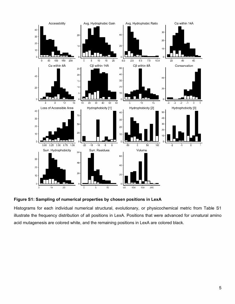
Figure S1: Sampling of numerical properties by chosen positions in LexA
Histograms for each individual numerical structural, evolutionary, or physicochemical metric from Table S1
illustrate the frequency distribution of all positions in LexA. Positions that were advanced for unnatural amino
acid mutagenesis are colored white, and the remaining positions in LexA are colored black.
6
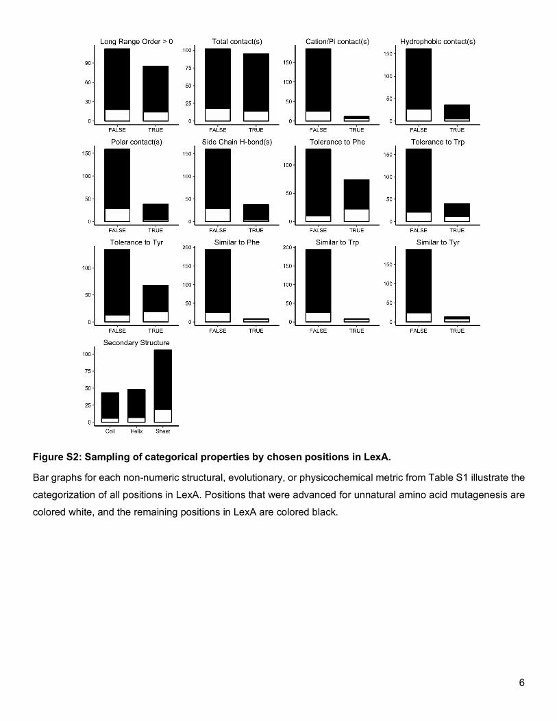
Figure S2: Sampling of categorical properties by chosen positions in LexA.
Bar graphs for each non-numeric structural, evolutionary, or physicochemical metric from Table S1 illustrate the
categorization of all positions in LexA. Positions that were advanced for unnatural amino acid mutagenesis are
colored white, and the remaining positions in LexA are colored black.
7
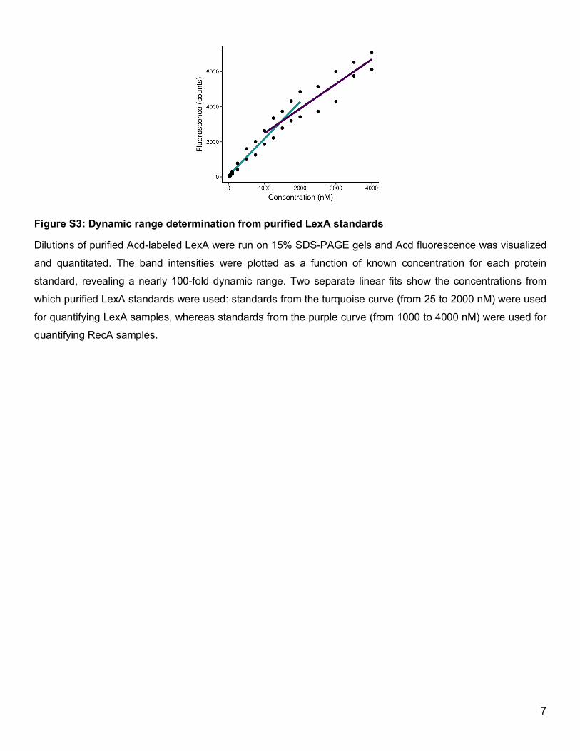
Figure S3: Dynamic range determination from purified LexA standards
Dilutions of purified Acd-labeled LexA were run on 15% SDS-PAGE gels and Acd fluorescence was visualized
and quantitated. The band intensities were plotted as a function of known concentration for each protein
standard, revealing a nearly 100-fold dynamic range. Two separate linear fits show the concentrations from
which purified LexA standards were used: standards from the turquoise curve (from 25 to 2000 nM) were used
for quantifying LexA samples, whereas standards from the purple curve (from 1000 to 4000 nM) were used for
quantifying RecA samples.
8
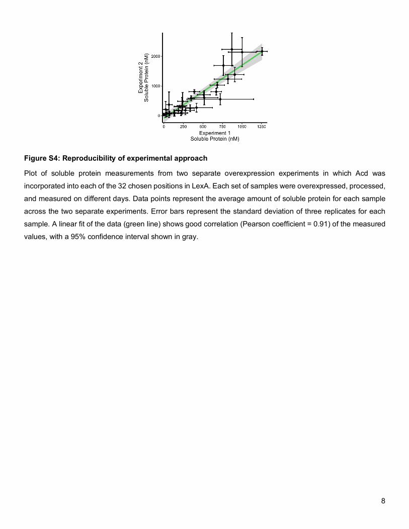
Figure S4: Reproducibility of experimental approach
Plot of soluble protein measurements from two separate overexpression experiments in which Acd was
incorporated into each of the 32 chosen positions in LexA. Each set of samples were overexpressed, processed,
and measured on different days. Data points represent the average amount of soluble protein for each sample
across the two separate experiments. Error bars represent the standard deviation of three replicates for each
sample. A linear fit of the data (green line) shows good correlation (Pearson coefficient = 0.91) of the measured
values, with a 95% confidence interval shown in gray.
9
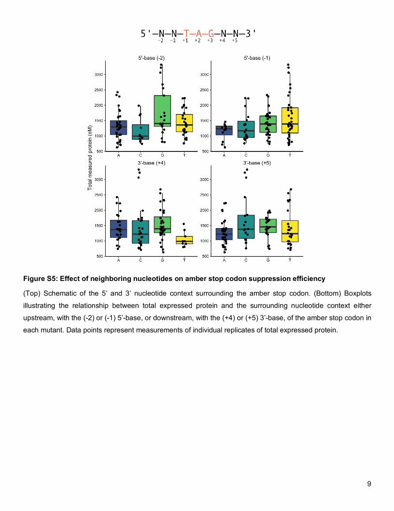
Figure S5: Effect of neighboring nucleotides on amber stop codon suppression efficiency
(Top) Schematic of the 5’ and 3’ nucleotide context surrounding the amber stop codon. (Bottom) Boxplots
illustrating the relationship between total expressed protein and the surrounding nucleotide context either
upstream, with the (-2) or (-1) 5’-base, or downstream, with the (+4) or (+5) 3’-base, of the amber stop codon in
each mutant. Data points represent measurements of individual replicates of total expressed protein.
10
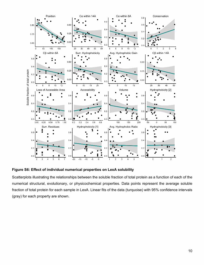
Figure S6: Effect of individual numerical properties on LexA solubility
Scatterplots illustrating the relationships between the soluble fraction of total protein as a function of each of the
numerical structural, evolutionary, or physicochemical properties. Data points represent the average soluble
fraction of total protein for each sample in LexA. Linear fits of the data (turquoise) with 95% confidence intervals
(gray) for each property are shown.
11
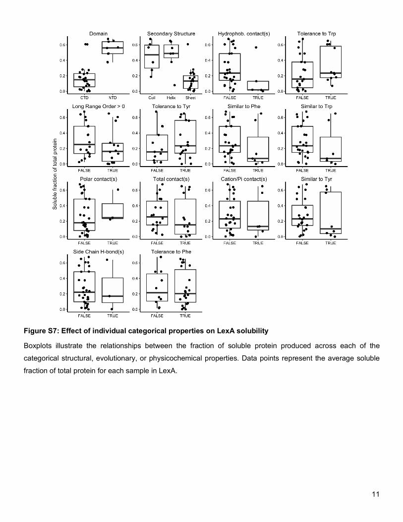
Figure S7: Effect of individual categorical properties on LexA solubility
Boxplots illustrate the relationships between the fraction of soluble protein produced across each of the
categorical structural, evolutionary, or physicochemical properties. Data points represent the average soluble
fraction of total protein for each sample in LexA.
12
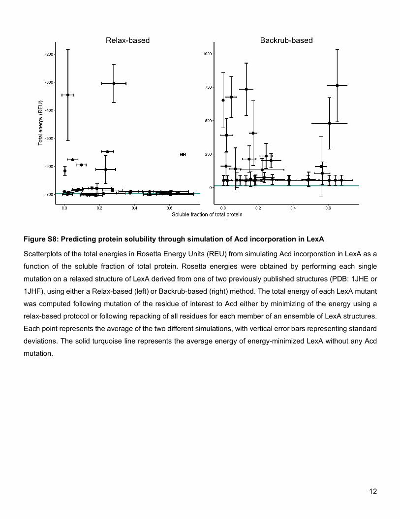
Figure S8: Predicting protein solubility through simulation of Acd incorporation in LexA
Scatterplots of the total energies in Rosetta Energy Units (REU) from simulating Acd incorporation in LexA as a
function of the soluble fraction of total protein. Rosetta energies were obtained by performing each single
mutation on a relaxed structure of LexA derived from one of two previously published structures (PDB: 1JHE or
1JHF), using either a Relax-based (left) or Backrub-based (right) method. The total energy of each LexA mutant
was computed following mutation of the residue of interest to Acd either by minimizing of the energy using a
relax-based protocol or following repacking of all residues for each member of an ensemble of LexA structures.
Each point represents the average of the two different simulations, with vertical error bars representing standard
deviations. The solid turquoise line represents the average energy of energy-minimized LexA without any Acd
mutation.
13
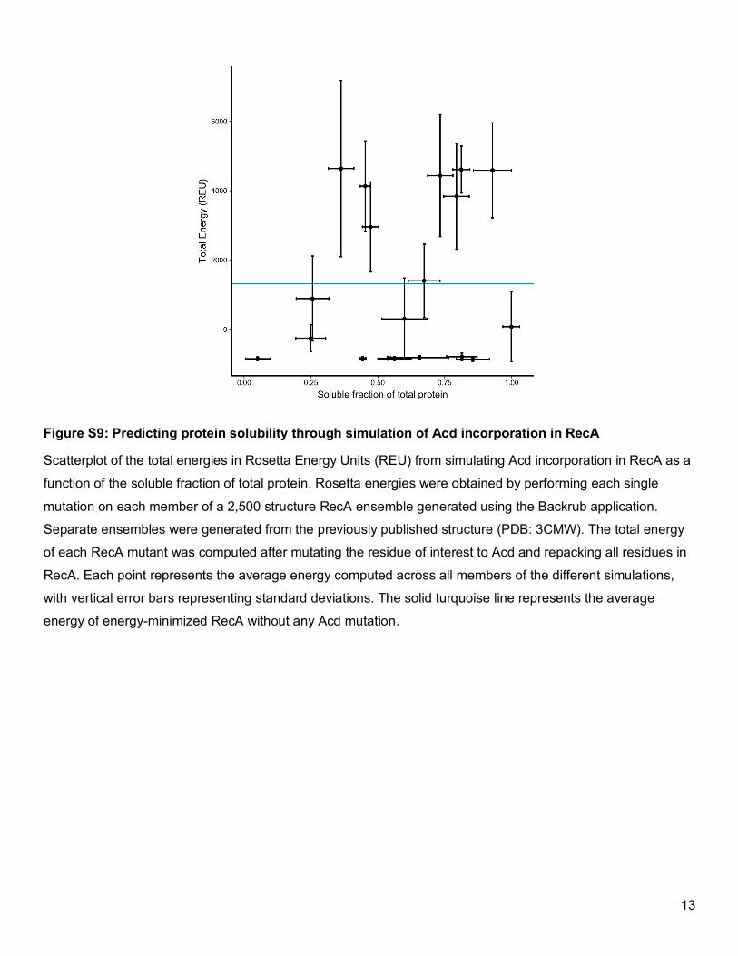
Figure S9: Predicting protein solubility through simulation of Acd incorporation in RecA
Scatterplot of the total energies in Rosetta Energy Units (REU) from simulating Acd incorporation in RecA as a
function of the soluble fraction of total protein. Rosetta energies were obtained by performing each single
mutation on each member of a 2,500 structure RecA ensemble generated using the Backrub application.
Separate ensembles were generated from the previously published structure (PDB: 3CMW). The total energy
of each RecA mutant was computed after mutating the residue of interest to Acd and repacking all residues in
RecA. Each point represents the average energy computed across all members of the different simulations,
with vertical error bars representing standard deviations. The solid turquoise line represents the average
energy of energy-minimized RecA without any Acd mutation.
14
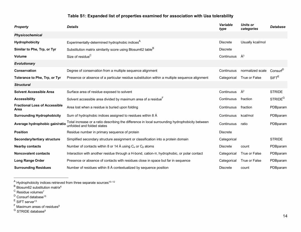
Table S1: Expanded list of properties examined for association with Uaa tolerability
Property Details Variable type
Units or categories Database
Physicochemical
Hydrophobicity Experimentally-determined hydrophobic indicesA Discrete Usually kcal/mol
Similar to Phe, Trp, or Tyr Substitution matrix similarity score using Blosum62 tableB Discrete
Volume Size of residueC Continuous Å3
Evolutionary
Conservation Degree of conservation from a multiple sequence alignment Continuous normalized scale ConsurfD
Tolerance to Phe, Trp, or Tyr Presence or absence of a particular residue substitution within a multiple sequence alignment Categorical True or False SIFTE
Structural
Solvent Accessible Area Surface area of residue exposed to solvent Continuous Å2 STRIDE
Accessibility Solvent accessible area divided by maximum area of a residueF Continuous fraction STRIDEG
Fractional Loss of Accessible Area Area lost when a residue is buried upon folding Continuous fraction PDBparam
Surrounding Hydrophobicity Sum of hydrophobic indices assigned to residues within 8 Å Continuous kcal/mol PDBparam
Average hydrophobic gain/ratio Total increase or a ratio describing the difference in local surrounding hydrophobicity between unfolded and folded states Continuous ratio PDBparam
Position Residue number in primary sequence of protein Discrete
Secondary/tertiary structure Simplified secondary structure assignment or classification into a protein domain Categorical STRIDE
Nearby contacts Number of contacts within 8 or 14 Å using Cα or Cβ atoms Discrete count PDBparam
Noncovalent contacts Interaction with another residue through a H-bond, cation-π, hydrophobic, or polar contact Categorical True or False PDBparam
Long Range Order Presence or absence of contacts with residues close in space but far in sequence Categorical True or False PDBparam
Surrounding Residues Number of residues within 8 Å contextualized by sequence position Discrete count PDBparam
A Hydrophobicity indices retrieved from three separate sources10–12 B Blosum62 substitution matrix6 C Residue volumes7 D Consurf database15 E SIFT server13 F Maximum areas of residues8 G STRIDE database9
15
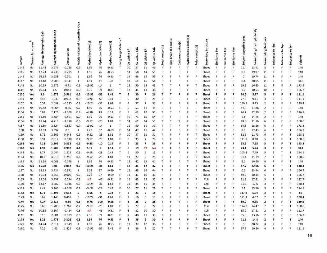
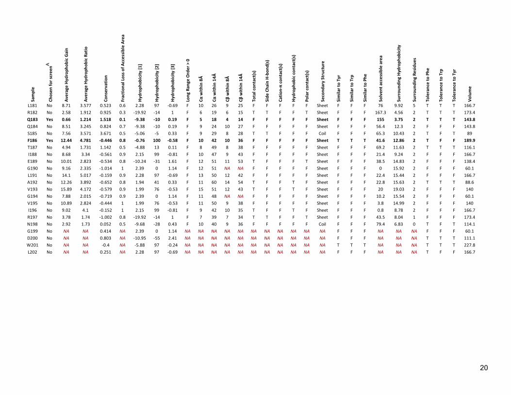
Table S2: Properties assigned to each position in LexA Sa
mpl
e
Chos
en fo
r scr
eenA
Aver
age
Hydr
opho
bic G
ain
Aver
age
Hydr
opho
bic R
atio
Cons
erva
tion
Frac
tiona
l Los
s of A
cces
sible
Are
a
Hydr
opho
bici
ty [1
]
Hydr
opho
bici
ty [2
]
Hydr
opho
bici
ty [3
]
Long
Ran
ge O
rder
> 0
Cα w
ithin
8Å
Cα w
ithin
14Å
Cβ w
ithin
8Å
Cβ w
ithin
14Å
Tota
l con
tact
(s)
Side
Cha
in H
-bon
d(s)
Catio
n -π
cont
act(
s)
Hydr
opho
bic c
onta
ct(s
)
Pola
r con
tact
(s)
Seco
ndar
y St
ruct
ure
Sim
ilar t
o Ty
r
Sim
ilar t
o Tr
p
Sim
ilar t
o Ph
e
Solv
ent a
cces
sible
are
a
Surr
ound
ing
Hydr
opho
bici
ty
Surr
ound
ing
Resid
ues
Tole
ranc
e to
Phe
Tole
ranc
e to
Trp
Tole
ranc
e to
Tyr
Volu
me
M1 No NA NA -0.794 NA -1.48 74 -0.44 NA NA NA NA NA NA NA NA NA NA NA F F F NA NA NA T F F 162.9 K2 No 1.64 1.539 1.15 0 -9.52 -23 1.81 F 2 23 5 25 T F T F T Coil F F F 201 3.04 2 T T T 168.6 A3 No 2.51 1.647 1.014 0.4 1.94 41 0.33 T 4 21 4 17 F F F F F Coil F F F 69.8 5.52 3 T F T 88.6 L4 No 6.83 2.98 -0.646 0.8 2.28 97 -0.69 T 9 25 11 30 F F F F F Coil F F F 37.6 8.11 7 F F F 166.7 T5 No 0.07 1.015 -0.66 0.5 -4.88 13 0.11 F 6 23 6 23 T T F F F Coil F F F 70.4 4.76 4 F F F 116.1 A6 Yes 1.54 1.498 1.377 0.2 1.94 41 0.33 F 6 19 7 19 F F F F F Helix F F F 83.3 3.76 4 F F F 88.6 R7 No 5.56 6.915 -0.547 0.6 -19.92 -14 1 F 7 31 8 30 T F T F T Helix F F F 100.2 5.65 4 F F F 173.4 Q8 No 13.06 6.464 -0.938 0.9 -9.38 -10 0.19 T 12 38 13 34 T T F F F Helix F F F 19.6 15.45 8 F F F 143.8 Q9 Yes 6.64 2.959 1.073 0.6 -9.38 -10 0.19 F 9 36 10 28 F F F F F Helix F F F 72 10.03 4 F F F 143.8 E10 No 5.22 2.101 0.737 0.4 -10.24 -31 1.61 F 8 40 10 34 T F F F T Helix F F F 98.5 9.29 4 F F F 138.4 V11 No 16.4 4.905 -0.52 1 1.99 76 -0.53 T 12 54 15 49 F F F F F Helix F F F 0 18.73 8 F F F 140 F12 Yes 9.04 2.683 -0.233 0.9 -0.76 100 -0.58 T 9 54 13 49 T F T F F Helix T T T 24.5 11.54 5 T T T 189.9 D13 No 2.84 1.282 1.378 0.7 -10.95 -55 2.41 T 9 48 11 43 T T F F T Helix F F F 39.3 12.24 5 F F F 111.1 L14 No 9.39 2.247 0.075 0.9 2.28 97 -0.69 T 9 54 13 47 F F F F F Helix F F F 14.8 14.75 5 T T F 166.7 I15 No 17.45 5.021 -0.803 1 2.15 99 -0.81 F 10 54 16 56 F F F F F Helix F F F 0 18.64 6 F F F 166.7 R16 No 11.24 2.641 0.286 0.8 -19.92 -14 1 T 11 45 11 47 T T T F T Helix F F F 54.2 17.24 7 F F F 173.4 D17 No 10.04 2.252 2.009 0.8 -10.95 -55 2.41 T 13 42 13 38 T T F F F Helix F F F 21.8 17.4 9 T T T 111.1 H18 No 13.57 3.869 0.7 0.8 -10.27 8 1.37 F 12 42 13 41 T T F F T Helix T F F 34.8 17.43 8 T T T 153.2 I19 No 14.53 10.081 -0.054 0.8 2.15 99 -0.81 F 11 35 11 36 F F F F F Helix F F F 41.2 12.98 7 F F F 166.7 S20 No 9.16 3.24 1.946 0.5 -5.06 -5 0.33 T 11 38 10 36 T T F F F Helix F F F 56.4 13.18 7 T F T 89 Q21 Yes 4.97 2.466 1.977 0.4 -9.38 -10 0.19 T 8 32 9 33 F F F F F Helix F F F 109.2 8.36 4 T T T 143.8 T22 Yes 6.86 4.728 0.172 0.5 -4.88 13 0.11 F 7 25 5 26 T T F F F Helix F F F 64.7 8.63 3 T F T 116.1 G23 No 4.19 1.929 -0.965 0.2 2.39 0 1.14 F 7 24 NA NA F F F F F Coil F F F 62.9 8.6 2 F F F 60.1 M24 No 6.61 2.158 -0.18 0.6 -1.48 74 -0.44 T 8 31 7 25 F F F F F Coil F F F 87.8 10.65 3 T T T 162.9 P25 No 15.81 4.43 -0.657 0.9 NA -46 -0.31 T 13 44 10 42 T F F T F Coil F F F 17.2 17.65 6 F F F 112.7 P26 No 14.61 3.726 -0.994 1 NA -46 -0.31 T 10 42 12 43 F F F F F Coil F F F 0.6 17.2 5 F F F 112.7 T27 No 4.81 1.663 -0.904 0.8 -4.88 13 0.11 T 8 44 9 34 T T F F F Coil F F F 26.5 12 6 F F F 116.1 R28 No 10.12 3.311 -0.557 0.8 -19.92 -14 1 T 11 45 10 39 T T F F T Helix F F F 54.2 13.65 9 T F F 173.4 A29 No 5.45 2.15 -0.788 0.5 1.94 41 0.33 T 9 31 9 28 F F F F F Helix F F F 56.3 9.32 7 F F F 88.6 E30 No 4.36 1.76 -0.879 0.6 -10.24 -31 1.61 F 8 38 10 34 T T F F T Helix F F F 63.9 9.43 4 F F F 138.4 I31 No 20.41 9.469 -0.915 1 2.15 99 -0.81 T 14 43 17 46 T F F T F Helix F F F 0 19.67 7 F F F 166.7 A32 No 13.16 3.818 -0.438 0.9 1.94 41 0.33 F 14 33 14 27 T F F T F Helix F F F 7.5 16.96 10 F F F 88.6
A Rows containing chosen positions are also indicated in bold type
16
Sam
ple
Chos
en fo
r scr
eenA
Aver
age
Hydr
opho
bic G
ain
Aver
age
Hydr
opho
bic R
atio
Cons
erva
tion
Frac
tiona
l Los
s of A
cces
sible
Are
a
Hydr
opho
bici
ty [1
]
Hydr
opho
bici
ty [2
]
Hydr
opho
bici
ty [3
]
Long
Ran
ge O
rder
> 0
Cα w
ithin
8Å
Cα w
ithin
14Å
Cβ w
ithin
8Å
Cβ w
ithin
14Å
Tota
l con
tact
(s)
Side
Cha
in H
-bon
d(s)
Catio
n-π
cont
act(
s)
Hydr
opho
bic c
onta
ct(s
)
Pola
r con
tact
(s)
Seco
ndar
y St
ruct
ure
Sim
ilar t
o Ty
r
Sim
ilar t
o Tr
p
Sim
ilar t
o Ph
e
Solv
ent a
cces
sible
are
a
Surr
ound
ing
Hydr
opho
bici
ty
Surr
ound
ing
Resid
ues
Tole
ranc
e to
Phe
Tole
ranc
e to
Trp
Tole
ranc
e to
Tyr
Volu
me
Q33 Yes 4.51 1.641 1.357 0.2 -9.38 -10 0.19 F 8 25 8 24 F F F F F Helix F F F 151.7 11.55 4 T F T 143.8 R34 No 7.54 3.401 -0.276 0.3 -19.92 -14 1 F 7 29 8 35 T F F F T Helix F F F 150.2 9.83 3 T T T 173.4 L35 No 8.06 3.11 -0.493 0.7 2.28 97 -0.69 F 7 34 10 36 F F F F F Helix F F F 53.5 9.71 2 T F F 166.7 G36 Yes 0.97 1.144 -0.399 0.3 2.39 0 1.14 F 6 23 NA NA F F F F F Coil F F F 57.3 7.61 2 F F F 60.1 F37 Yes 12.25 4.84 -0.699 0.9 -0.76 100 -0.58 F 11 26 10 29 T F T T F Coil T T T 17.4 12.57 5 T F T 189.9 R38 No 2.59 1.446 -0.005 0.2 -19.92 -14 1 F 6 20 6 19 T F T F F Coil F F F 189 7.55 3 F F T 173.4 S39 No 3.55 1.54 -0.939 0.6 -5.06 -5 0.33 F 8 22 8 20 F F F F F Coil F F F 41.3 10.06 4 F F F 89 P40 No 12.92 7.872 -0.485 0.5 NA -46 -0.31 F 11 26 10 26 F F F F F Helix F F F 68.5 12.03 4 T F F 112.7 N41 No 2.28 1.498 -0.871 0.2 -9.68 -28 0.43 F 7 23 8 21 F F F F F Helix F F F 123.9 6.77 4 F F F 114.1 A42 No 7.07 2.607 -0.776 0.9 1.94 41 0.33 F 10 28 11 29 T F F T F Helix F F F 14.5 10.6 4 F F F 88.6 A43 No 15.36 7.678 -0.859 1 1.94 41 0.33 F 13 41 16 40 T F F T F Helix F F F 0 16.79 4 F F F 88.6 E44 No 8.19 3.497 -0.633 0.7 -10.24 -31 1.61 F 9 44 10 37 T T F F T Helix F F F 44.3 10.8 4 F F F 138.4 E45 No 4.14 1.904 -0.249 0.2 -10.24 -31 1.61 F 8 36 9 30 T F F F T Helix F F F 132.8 8.05 4 F F T 138.4 H46 No 7.52 2.46 -0.746 0.8 -10.27 8 1.37 F 10 46 13 44 T F F F T Helix T F F 38.5 11.8 4 F F T 153.2 L47 No 11.77 3.906 -0.682 1 2.28 97 -0.69 F 11 53 15 53 F F F F F Helix F F F 0 13.65 5 F F F 166.7 K48 No 7.85 2.291 0.436 0.5 -9.52 -23 1.81 F 9 37 10 31 T T F F T Helix F F F 104.8 12.29 5 F F F 168.6 A49 No 4.9 1.715 -0.456 1 1.94 41 0.33 F 9 33 10 33 F F F F F Helix F F F 4.8 10.88 4 F F F 88.6 L50 No 17.01 5.021 -0.943 1 2.28 97 -0.69 F 13 42 15 44 F F F F F Helix F F F 0 19.07 6 F F F 166.7 A51 No 13.62 3.463 -0.625 0.7 1.94 41 0.33 F 11 34 11 32 T F F T F Helix F F F 33.2 18.28 7 F F F 88.6 R52 No 5.23 2.094 0.081 0.2 -19.92 -14 1 F 7 29 6 24 F F F F F Helix F F F 179.6 9.16 3 F F F 173.4 K53 No 7.72 3.092 -0.656 0.6 -9.52 -23 1.81 F 8 28 10 28 T T F F F Helix F F F 78 9.77 2 F F F 168.6 G54 No 5.98 1.796 -0.94 0.7 2.39 0 1.14 T 8 29 NA NA F F F F F Coil F F F 23.8 13.39 4 F F F 60.1 V55 No 10.1 2.817 0.578 0.9 1.99 76 -0.53 T 10 37 11 37 F F F F F Coil F F F 8.8 13.79 5 T T T 140 I56 No 14.53 3.509 -0.57 1 2.15 99 -0.81 T 10 46 13 44 F F F F F Sheet F F F 2.5 17.17 6 F F F 166.7 E57 No 9.98 1.994 -0.188 0.6 -10.24 -31 1.61 T 10 34 9 26 T F F F T Sheet F F F 76.2 19.35 6 F F F 138.4 I58 No 11.93 3.071 -0.621 0.7 2.15 99 -0.81 F 10 34 10 32 T F F T F Sheet F F F 48.5 14.54 5 T F F 166.7 V59 No 6.84 2.714 0.076 0.6 1.99 76 -0.53 F 8 27 7 23 F F F F F Coil F F F 57.9 8.96 6 T T T 140 S60 Yes 0.17 1.028 0.413 0.1 -5.06 -5 0.33 F 5 20 4 16 F F F F F Coil F F F 105.8 6.09 3 F F F 89 G61 No 0.2 1.069 -0.383 0.2 2.39 0 1.14 F 5 17 NA NA F F F F F Coil F F F 57.9 2.98 3 F F F 60.1 A62 No 2.84 3.606 -0.408 0.2 1.94 41 0.33 F 6 16 5 14 F F F F F Sheet F F F 82.8 3.06 3 T F T 88.6 S63 No 0.14 1.073 -0.709 0.2 -5.06 -5 0.33 F 5 22 4 22 F F F F F Sheet F F F 98.7 1.99 2 F F F 89 R64 No 8.98 3.143 -1.019 0.7 -19.92 -14 1 F 9 33 8 29 T T F F T Sheet F F F 77.8 12.32 2 F F F 173.4 G65 No 8.93 2.815 -0.772 0.9 2.39 0 1.14 F 10 34 NA NA F F F F F Sheet F F F 7.7 13.75 2 F F F 60.1 I66 No 14.76 4.718 -0.584 1 2.15 99 -0.81 F 9 48 12 46 T F F T F Sheet F F F 7.8 15.58 2 F F F 166.7 R67 No 12.46 2.642 -0.538 0.4 -19.92 -14 1 F 9 42 9 26 T F F F T Sheet F F F 138.7 19.2 2 F F F 173.4 L68 No 8.53 2.382 -0.234 0.8 2.28 97 -0.69 F 8 38 12 36 F F F F F Sheet F F F 36.1 12.53 3 F F F 166.7 L69 No 7.96 3.157 0.859 0.6 2.28 97 -0.69 F 8 27 8 25 F F F F F Sheet F F F 71.4 9.48 2 T T T 166.7
17
Sam
ple
Chos
en fo
r scr
eenA
Aver
age
Hydr
opho
bic G
ain
Aver
age
Hydr
opho
bic R
atio
Cons
erva
tion
Frac
tiona
l Los
s of A
cces
sible
Are
a
Hydr
opho
bici
ty [1
]
Hydr
opho
bici
ty [2
]
Hydr
opho
bici
ty [3
]
Long
Ran
ge O
rder
> 0
Cα w
ithin
8Å
Cα w
ithin
14Å
Cβ w
ithin
8Å
Cβ w
ithin
14Å
Tota
l con
tact
(s)
Side
Cha
in H
-bon
d(s)
Catio
n-π
cont
act(
s)
Hydr
opho
bic c
onta
ct(s
)
Pola
r con
tact
(s)
Seco
ndar
y St
ruct
ure
Sim
ilar t
o Ty
r
Sim
ilar t
o Tr
p
Sim
ilar t
o Ph
e
Solv
ent a
cces
sible
are
a
Surr
ound
ing
Hydr
opho
bici
ty
Surr
ound
ing
Resid
ues
Tole
ranc
e to
Phe
Tole
ranc
e to
Trp
Tole
ranc
e to
Tyr
Volu
me
Q70 No 2.54 1.447 3.837 0.3 -9.38 -10 0.19 F 6 20 7 23 F F F F F Sheet F F F 119.7 8.22 3 T T T 143.8 E71 No 2.84 1.809 3.353 0.2 -10.24 -31 1.61 F 5 28 6 26 F F F F F Sheet F F F 146.3 5.68 2 T T T 138.4 E72 No 0.67 1.333 3.827 -0.1 -10.24 -31 1.61 F 4 22 4 15 F F F F F Coil F F F 198.2 2.01 2 T F T 138.4 E73 No 0.67 1.318 3.73 0.3 -10.24 -31 1.61 F 5 25 6 29 T F F F T Coil F F F 119.8 2.11 2 T T T 138.4 E74 Yes 0.67 1.186 3.844 0.2 -10.24 -31 1.61 T 5 23 4 22 F F F F F Coil F F F 138 3.61 3 T T T 138.4 G75 No 8.94 2.424 1.324 0.9 2.39 0 1.14 T 10 32 NA NA F F F F F Coil F F F 7.5 15.12 8 F F F 60.1 L76 No 16.92 3.963 -0.222 1 2.28 97 -0.69 T 13 42 12 40 F F F F F Sheet F F F 2.8 20.46 11 F F F 166.7 P77 No 15.93 3.525 -0.927 0.8 NA -46 -0.31 T 12 42 9 44 T F F T F Sheet F F F 24.7 19.47 10 F F F 112.7 L78 No 19.86 3.874 0.197 1 2.28 97 -0.69 T 14 48 13 42 T F F T F Sheet F F F 1.8 24.6 12 F F F 166.7 V79 No 20.93 4.553 -0.013 1 1.99 76 -0.53 T 15 49 13 46 T F F T F Sheet F F F 0 24.95 13 F F F 140 G80 No 7.81 2.155 -1.015 0.9 2.39 0 1.14 T 9 41 NA NA F F F F F Coil F F F 6.4 14.47 7 F F F 60.1 R81 Yes 2.57 1.546 0.136 0.1 -19.92 -14 1 T 6 39 5 30 F F F F F Coil F F F 211.7 6.43 4 F F F 173.4 V82 No 9.32 4.465 -0.902 0.8 1.99 76 -0.53 T 9 39 10 41 F F F F F Coil F F F 31.3 10.14 6 F F F 140 A83 No 3.07 1.832 -0.874 0.7 1.94 41 0.33 T 7 29 8 24 F F F F F Sheet F F F 32.6 5.89 5 F F F 88.6 A84 No 2.2 1.627 -1.021 0.4 1.94 41 0.33 T 6 27 4 22 F F F F F Sheet F F F 70.7 4.84 4 F F F 88.6 G85 No 0.76 1.147 -0.99 0.4 2.39 0 1.14 T 5 29 NA NA F F F F F Sheet F F F 47.3 5.84 3 F F F 60.1 E86 Yes 4.94 1.836 1.116 0.8 -10.24 -31 1.61 F 9 36 11 32 T F F F T Sheet F F F 39 10.18 3 T T T 138.4 P87 No 4.37 1.855 -0.883 0.9 NA -46 -0.31 F 8 46 8 40 T F F T F Sheet F F F 13 6.71 3 F F F 112.7 L88 No 7.45 2.15 -0.746 1 2.28 97 -0.69 T 8 58 13 54 F F F F F Sheet F F F 6.3 11.76 4 F F F 166.7 L89 No 8.79 2.513 -0.421 0.8 2.28 97 -0.69 F 9 53 10 46 F F F F F Sheet F F F 42.8 12.43 4 T T T 166.7 A90 No 9.91 3.283 -0.953 1 1.94 41 0.33 F 11 42 14 37 T F F T F Sheet F F F 0 13.38 4 F F F 88.6 Q91 No 5.32 2.361 0.066 0.7 -9.38 -10 0.19 F 8 39 8 41 F F F F F Helix F F F 50.3 9.23 3 T F T 143.8 Q92 No 0.67 1.137 -0.274 0.3 -9.38 -10 0.19 F 5 34 8 29 F F F F F Helix F F F 120.5 5.56 3 T F T 143.8 H93 No 11.64 4.047 0.063 1 -10.27 8 1.37 F 12 37 13 38 T F F F T Helix T F F 7.6 14.59 2 T F T 153.2 I94 No 13.97 9.518 0.209 0.8 2.15 99 -0.81 F 12 34 11 33 T F F T F Sheet F F F 32.9 12.46 3 T F F 166.7 E95 No 7.58 2.519 0.158 0.4 -10.24 -31 1.61 F 9 29 6 28 T T F F T Sheet F F F 104.9 11.9 2 F F F 138.4 G96 No 6.91 1.939 0.611 0.7 2.39 0 1.14 F 7 30 NA NA F F F F F Sheet F F F 22.8 14.17 2 T T T 60.1 H97 Yes 11.23 4.265 0.831 0.5 -10.27 8 1.37 F 9 36 9 31 T F F F T Sheet T F F 86.5 13.8 2 T T T 153.2 Y98 Yes 9.88 4.479 0.274 0.7 -6.11 63 0.23 F 10 34 9 34 T F T F F Sheet T T T 67.4 10.05 2 T T T 193.6 Q99 No 2.94 1.484 0.873 0.4 -9.38 -10 0.19 F 8 26 6 22 F F F F F Sheet F F F 101.5 9.01 2 T T T 143.8 V100 No 4.14 1.679 0.074 1 1.99 76 -0.53 F 7 33 10 32 F F F F F Coil F F F 1.3 8.37 2 T F F 140 D101 No 2.93 1.622 -0.637 0.6 -10.95 -55 2.41 F 7 33 7 25 T T F F F Coil F F F 51.3 6.98 3 F F F 111.1 P102 No 9.53 2.998 1.822 0.7 NA -46 -0.31 F 10 39 10 32 F F F F F Helix F F F 36.5 11.53 6 F F F 112.7 S103 No 5.44 1.642 1.219 0.4 -5.06 -5 0.33 F 8 32 7 22 T T F F F Helix F F F 69.4 13.84 6 T F T 89 L104 Yes 2.92 1.397 0.453 0.9 2.28 97 -0.69 T 8 36 11 32 F F F F F Helix F F F 22.1 8.1 3 T F T 166.7 F105 Yes 9.44 2.42 0.141 1 -0.76 100 -0.58 T 12 35 12 34 T F F T F Sheet T T T 1.8 13.22 7 T F F 189.9 K106 Yes 4.45 1.563 1.12 0.1 -9.52 -23 1.81 T 9 32 7 22 F F F F F Sheet F F F 176.8 10.71 4 T T T 168.6
18
Sam
ple
Chos
en fo
r scr
eenA
Aver
age
Hydr
opho
bic G
ain
Aver
age
Hydr
opho
bic R
atio
Cons
erva
tion
Frac
tiona
l Los
s of A
cces
sible
Are
a
Hydr
opho
bici
ty [1
]
Hydr
opho
bici
ty [2
]
Hydr
opho
bici
ty [3
]
Long
Ran
ge O
rder
> 0
Cα w
ithin
8Å
Cα w
ithin
14Å
Cβ w
ithin
8Å
Cβ w
ithin
14Å
Tota
l con
tact
(s)
Side
Cha
in H
-bon
d(s)
Catio
n-π
cont
act(
s)
Hydr
opho
bic c
onta
ct(s
)
Pola
r con
tact
(s)
Seco
ndar
y St
ruct
ure
Sim
ilar t
o Ty
r
Sim
ilar t
o Tr
p
Sim
ilar t
o Ph
e
Solv
ent a
cces
sible
are
a
Surr
ound
ing
Hydr
opho
bici
ty
Surr
ound
ing
Resid
ues
Tole
ranc
e to
Phe
Tole
ranc
e to
Trp
Tole
ranc
e to
Tyr
Volu
me
P107 No 5.58 2.02 1.33 0.7 NA -46 -0.31 T 7 33 9 31 F F F F F Sheet F F F 45.1 8.28 4 F F T 112.7 N108 Yes 10.71 2.803 1.131 0.4 -9.68 -28 0.43 T 10 35 10 28 T T F F F Sheet F F F 81.9 16.56 4 T T T 114.1 A109 No 19.68 4.08 0.293 1 1.94 41 0.33 T 15 47 15 42 T F F T F Coil F F F 3.4 25.2 8 T F T 88.6 D110 No 13.62 3.27 -0.273 0.5 -10.95 -55 2.41 T 11 51 9 46 T T F F T Coil F F F 72.9 18.96 6 F F F 111.1 F111 Yes 17.1 3.913 -0.453 1 -0.76 100 -0.58 T 12 60 12 51 T F T T F Sheet T T T 2.4 20.1 6 T F T 189.9 L112 No 19.1 3.916 -0.38 1 2.28 97 -0.69 T 13 61 16 49 T F F T F Sheet F F F 0 23.48 6 T F F 166.7 L113 No 13.39 2.726 -0.991 1 2.28 97 -0.69 T 11 63 13 57 T F F T F Sheet F F F 7.4 18.98 6 F F F 166.7 R114 No 10.94 2.742 0.024 0.6 -19.92 -14 1 T 12 54 12 40 T T T F T Sheet F F F 101.8 16.37 6 F F F 173.4 V115 No 14.32 5.489 -0.811 0.9 1.99 76 -0.53 T 12 51 12 46 F F F F F Sheet F F F 11.5 15.64 10 F F F 140 S116 No 2.5 1.557 0.615 0 -5.06 -5 0.33 T 7 39 4 33 F F F F F Coil F F F 111 6.92 5 F F T 89 G117 No 4.2 1.937 -0.99 0.7 2.39 0 1.14 F 8 35 NA NA F F F F F Coil F F F 25.7 8.58 6 F F F 60.1 M118 No 8.88 4.277 -0.001 0.7 -1.48 74 -0.44 T 9 32 9 26 F F F F F Sheet F F F 58.5 9.92 7 T T T 162.9 A119 No 8.91 2.754 -1.011 0.9 1.94 41 0.33 T 9 38 11 40 T F F T F Sheet F F F 8.3 13.12 7 F F F 88.6 M120 No 16.88 4.488 -1.02 1 -1.48 74 -0.44 T 14 44 14 44 T F F T F Sheet F F F 5.4 20.05 11 F F F 162.9 K121 No 8.99 2.416 -0.553 0.8 -9.52 -23 1.81 T 10 32 10 26 T F F F T Helix F F F 50 13.7 7 F F T 168.6 D122 No 4.57 1.697 0.189 0.4 -10.95 -55 2.41 T 8 25 7 24 T F F F T Helix F F F 88.1 10.47 5 F F F 111.1 I123 No 5.49 1.989 -0.553 0.7 2.15 99 -0.81 T 6 36 8 29 F F F F F Helix F F F 48.2 7.89 3 T T T 166.7 G124 No 3.41 1.395 -0.779 1 2.39 0 1.14 F 7 34 NA NA F F F F F Coil F F F 0 11.94 2 F F F 60.1 I125 No 13.19 3.364 -1.008 1 2.15 99 -0.81 T 11 41 12 39 T F F T F Coil F F F 9.8 15.62 4 F F F 166.7
M126 No 9.35 3.332 0.948 0.9 -1.48 74 -0.44 F 12 33 9 28 F F F F F Sheet F F F 24.7 11.69 3 T F T 162.9 D127 No 4.37 1.783 -0.474 0.3 -10.95 -55 2.41 F 8 32 6 28 T T F F F Sheet F F F 97.1 9.29 2 F F F 111.1 G128 No 3.84 1.744 -0.678 0.6 2.39 0 1.14 T 9 34 NA NA F F F F F Sheet F F F 31.7 8.9 3 F F F 60.1 D129 No 14.16 3.776 -1.019 1 -10.95 -55 2.41 T 12 39 11 38 T T F F T Sheet F F F 2.6 18.6 6 F F F 111.1 L130 Yes 17.36 5.568 0.482 1 2.28 97 -0.69 T 13 51 13 42 T F F T F Sheet F F F 4.2 18.99 6 F F F 166.7 L131 No 17.09 4.068 -0.556 1 2.28 97 -0.69 T 13 62 14 56 T F F T F Sheet F F F 1.2 20.49 7 F F F 166.7 A132 No 20.34 3.873 -0.404 1 1.94 41 0.33 T 15 57 14 46 T F F T F Sheet F F F 0 26.55 7 F F F 88.6 V133 No 17.59 4.169 -0.746 1 1.99 76 -0.53 T 15 60 15 57 F F F F F Sheet F F F 0 21.27 8 F F F 140 H134 No 13.14 3.953 -0.283 0.7 -10.27 8 1.37 T 13 47 13 41 T T F F T Sheet T F F 48.9 16.72 6 F F F 153.2 K135 Yes 8.98 4.196 0.396 0.4 -9.52 -23 1.81 T 10 45 7 40 T F T F F Sheet F F F 119.1 10.15 5 F F F 168.6 T136 No 8.03 3.533 0.056 0.7 -4.88 13 0.11 T 9 31 9 32 T T F F F Coil F F F 38.1 11.13 7 F F F 116.1 Q137 No 3.99 1.941 1.468 0.1 -9.38 -10 0.19 T 8 28 6 24 F F F F F Coil F F F 154.1 8.23 6 T T T 143.8 D138 Yes 0.66 1.237 0.715 0 -10.95 -55 2.41 F 4 26 4 22 F F F F F Coil F F F 138.2 2.79 2 T F F 111.1 V139 No 5.98 4.737 -0.769 0.9 1.99 76 -0.53 T 8 33 10 32 F F F F F Coil F F F 19.3 5.71 5 F F F 140 R140 Yes 3.02 2.11 1.226 0.3 -19.92 -14 1 T 6 32 5 22 F F F F F Sheet F F F 170 4.89 4 F F F 173.4 N141 No 6.39 3.266 -0.454 0.5 -9.68 -28 0.43 T 8 29 6 22 F F F F F Sheet F F F 78.7 9.12 6 F F F 114.1 G142 No 4.76 2.694 -0.94 0.5 2.39 0 1.14 T 7 31 NA NA F F F F F Sheet F F F 35 7.47 5 F F F 60.1 Q143 No 7.91 3.013 -0.285 0.7 -9.38 -10 0.19 T 9 41 10 36 F F F F F Sheet F F F 58.7 11.84 5 F F F 143.8
19
Sam
ple
Chos
en fo
r scr
eenA
Aver
age
Hydr
opho
bic G
ain
Aver
age
Hydr
opho
bic R
atio
Cons
erva
tion
Frac
tiona
l Los
s of A
cces
sible
Are
a
Hydr
opho
bici
ty [1
]
Hydr
opho
bici
ty [2
]
Hydr
opho
bici
ty [3
]
Long
Ran
ge O
rder
> 0
Cα w
ithin
8Å
Cα w
ithin
14Å
Cβ w
ithin
8Å
Cβ w
ithin
14Å
Tota
l con
tact
(s)
Side
Cha
in H
-bon
d(s)
Catio
n-π
cont
act(
s)
Hydr
opho
bic c
onta
ct(s
)
Pola
r con
tact
(s)
Seco
ndar
y St
ruct
ure
Sim
ilar t
o Ty
r
Sim
ilar t
o Tr
p
Sim
ilar t
o Ph
e
Solv
ent a
cces
sible
are
a
Surr
ound
ing
Hydr
opho
bici
ty
Surr
ound
ing
Resid
ues
Tole
ranc
e to
Phe
Tole
ranc
e to
Trp
Tole
ranc
e to
Tyr
Volu
me
V144 No 11.44 3.979 -0.725 0.9 1.99 76 -0.53 T 10 57 11 49 T F F T F Sheet F F F 21.4 13.41 8 F F F 140 V145 No 17.23 4.738 -0.795 1 1.99 76 -0.53 T 14 58 14 51 F F F F F Sheet F F F 0.8 19.97 11 F F F 140 V146 No 16.15 3.958 -0.901 1 1.99 76 -0.53 T 14 66 15 59 F F F F F Sheet F F F 0 19.74 11 F F F 140 A147 No 13.18 2.703 -0.941 1 1.94 41 0.33 T 13 61 16 56 F F F F F Sheet F F F 0.4 20.05 11 F F F 88.6 R148 No 10.95 2.672 -0.71 0.9 -19.92 -14 1 T 13 50 14 45 T T F F T Sheet F F F 19.6 16.65 11 F F F 173.4 I149 No 10.64 4.5 0.057 0.9 2.15 99 -0.81 T 12 41 13 38 F F F F F Sheet F F F 16 10.53 10 T F F 166.7 D150 Yes 3.6 1.675 0.561 0.5 -10.95 -55 2.41 T 7 30 7 26 T T F F F Sheet F F F 74.6 8.27 5 T F T 111.1 D151 No 3.42 1.539 0.037 0.5 -10.95 -55 2.41 T 9 30 8 25 T T F F T Sheet F F F 77.3 9.11 3 F F F 111.1 E152 No 5.54 2.699 -0.625 0.1 -10.24 -31 1.61 F 7 37 7 33 F F F F F Sheet F F F 150.3 8.13 2 F F F 138.4 V153 No 10.48 4.205 -0.86 0.7 1.99 76 -0.53 F 9 53 11 45 F F F F F Sheet F F F 44.2 11.88 2 F F F 140 T154 No 6.81 2.126 -1.009 0.8 -4.88 13 0.11 F 8 62 12 52 T T F F F Sheet F F F 24.2 12.79 2 F F F 116.1 V155 No 11.89 3.684 -0.801 0.9 1.99 76 -0.53 F 10 71 15 54 F F F F F Sheet F F F 13 14.45 2 F F F 140 K156 No 18.44 4.718 -1.018 0.9 -9.52 -23 1.81 T 14 61 14 51 T T T F F Sheet F F F 18.8 21.76 6 F F F 168.6 R157 No 11.89 2.624 -0.567 0.7 -19.92 -14 1 T 12 50 11 39 T T F F T Sheet F F F 64.5 18.36 5 T F F 173.4 L158 No 13.83 3.397 0.1 1 2.28 97 -0.69 F 14 47 15 42 F F F F F Sheet F F F 9.1 17.43 6 T T T 166.7 K159 No 8.71 2.869 0.448 0.6 -9.52 -23 1.81 F 10 37 11 31 T F F F T Sheet F F F 82.6 11.73 6 F F T 168.6 K160 No 5.91 2.512 -0.018 0.4 -9.52 -23 1.81 F 8 33 7 28 F F F F F Sheet F F F 111.9 8.18 5 F F T 168.6 Q161 Yes 4.18 2.205 0.833 0.5 -9.38 -10 0.19 F 7 23 7 23 F F F F F Sheet F F F 93.9 7.65 5 T F T 143.8 G162 Yes 1.97 1.585 0.987 0.1 2.39 0 1.14 F 5 19 NA NA F F F F F Sheet F F F 73.1 5.24 3 F F F 60.1 N163 No 3.77 2.044 1.225 0.3 -9.68 -28 0.43 T 7 20 6 15 F F F F F Sheet F F F 105.1 7.29 5 T T T 114.1 K164 No 10.7 4.919 1.256 0.6 -9.52 -23 1.81 T 11 27 9 25 T F F F T Sheet F F F 91.4 11.79 7 T T T 168.6 V165 No 13.99 4.061 -0.148 1 1.99 76 -0.53 T 13 42 13 41 T F F T F Sheet F F F 6.2 16.69 6 F F T 140 E166 Yes 15.78 3.01 0.012 0.7 -10.24 -31 1.61 T 12 41 12 32 T F F F T Sheet F F F 47.7 22.96 6 T T T 138.4 L167 No 18.13 3.424 -0.991 1 2.28 97 -0.69 T 12 48 16 44 T F F T F Sheet F F F 0.2 23.44 6 F F F 166.7 L168 No 16.03 3.553 0.006 0.7 2.28 97 -0.69 F 11 41 10 39 F F F F F Sheet F F F 49.9 20.14 5 T T T 166.7 P169 No 15.08 3.957 -0.594 0.9 NA -46 -0.31 F 11 43 13 37 T F F T F Coil F F F 21.2 17.41 5 F F F 112.7 E170 No 13.17 3.582 -0.616 0.7 -10.24 -31 1.61 F 11 35 11 35 T T F F T Coil F F F 51.6 17.6 3 F F F 138.4 N171 No 9.47 3.266 -1.008 0.9 -9.68 -28 0.43 F 10 27 11 28 T T F F F Sheet F F F 12 13.56 3 F F F 114.1 S172 Yes 1.71 1.398 0.632 0 -5.06 -5 0.33 F 5 21 5 15 F F F F F Sheet F F F 117.8 5.94 3 F F F 89 E173 No 0.67 1.143 0.459 0 -10.24 -31 1.61 F 4 16 5 17 F F F F F Sheet F F F 171.4 4.67 2 F F F 138.4 F174 Yes 7.27 2.412 -0.16 0.6 -0.76 100 -0.58 F 8 26 9 28 T F T T F Sheet T T T 89.9 9.55 2 T F T 189.9 K175 No 6.65 1.703 1.267 0.2 -9.52 -23 1.81 F 7 27 5 22 F F F F F Coil F F F 174.9 14.47 2 T T T 168.6 P176 No 10.55 2.107 -0.424 0.5 NA -46 -0.31 F 8 32 10 30 F F F F F Coil F F F 65.9 17.31 2 F F F 112.7 I177 No 8.16 2.001 -0.809 0.6 2.15 99 -0.81 F 7 40 11 39 T F F T F Sheet F F F 65.9 13.16 2 F F F 166.7 V178 Yes 8.22 1.973 0.802 0.5 1.99 76 -0.53 F 8 36 9 30 F F F F F Sheet F F F 71.6 14.8 2 T T T 140 V179 No 14.24 2.814 -0.149 1 1.99 76 -0.53 F 11 37 12 38 T F F T F Sheet F F F 0 20.22 4 F F F 140 D180 No 4.26 1.63 1.424 0.9 -10.95 -55 2.41 F 9 26 9 22 T T F F T Sheet F F F 17.8 10.36 4 F F F 111.1
20
Sam
ple
Chos
en fo
r scr
eenA
Aver
age
Hydr
opho
bic G
ain
Aver
age
Hydr
opho
bic R
atio
Cons
erva
tion
Frac
tiona
l Los
s of A
cces
sible
Are
a
Hydr
opho
bici
ty [1
]
Hydr
opho
bici
ty [2
]
Hydr
opho
bici
ty [3
]
Long
Ran
ge O
rder
> 0
Cα w
ithin
8Å
Cα w
ithin
14Å
Cβ w
ithin
8Å
Cβ w
ithin
14Å
Tota
l con
tact
(s)
Side
Cha
in H
-bon
d(s)
Catio
n-π
cont
act(
s)
Hydr
opho
bic c
onta
ct(s
)
Pola
r con
tact
(s)
Seco
ndar
y St
ruct
ure
Sim
ilar t
o Ty
r
Sim
ilar t
o Tr
p
Sim
ilar t
o Ph
e
Solv
ent a
cces
sible
are
a
Surr
ound
ing
Hydr
opho
bici
ty
Surr
ound
ing
Resid
ues
Tole
ranc
e to
Phe
Tole
ranc
e to
Trp
Tole
ranc
e to
Tyr
Volu
me
L181 No 8.71 3.577 0.523 0.6 2.28 97 -0.69 F 10 26 9 25 F F F F F Sheet F F F 76 9.92 5 T T T 166.7 R182 No 2.58 1.912 0.925 0.3 -19.92 -14 1 F 6 19 6 15 T T F F T Sheet F F F 167.3 4.56 2 T T T 173.4 Q183 Yes 0.66 1.214 1.518 0.1 -9.38 -10 0.19 F 5 18 4 14 F F F F F Sheet F F F 155 3.75 2 T T T 143.8 Q184 No 8.51 3.245 0.824 0.7 -9.38 -10 0.19 F 9 24 10 27 F F F F F Sheet F F F 56.4 12.3 2 F F F 143.8 S185 No 7.56 3.571 3.671 0.5 -5.06 -5 0.33 F 9 29 8 28 T T F F F Coil F F F 65.3 10.43 2 T F T 89 F186 Yes 12.44 4.781 -0.446 0.8 -0.76 100 -0.58 F 10 42 10 36 F F F F F Sheet T T T 41.6 12.86 2 T F F 189.9 T187 No 4.94 1.731 1.142 0.5 -4.88 13 0.11 F 8 49 8 38 F F F F F Sheet F F F 69.2 11.63 2 T T T 116.1 I188 No 8.68 3.34 -0.561 0.9 2.15 99 -0.81 F 10 47 9 43 F F F F F Sheet F F F 21.4 9.24 2 F F F 166.7 E189 No 10.01 2.823 -0.534 0.8 -10.24 -31 1.61 F 12 51 11 53 T F F F T Sheet F F F 38.5 14.83 2 F F F 138.4 G190 No 9.16 2.335 -1.014 1 2.39 0 1.14 F 12 51 NA NA F F F F F Sheet F F F 0 15.92 2 F F F 60.1 L191 No 14.1 5.017 -0.159 0.9 2.28 97 -0.69 F 13 50 12 42 F F F F F Sheet F F F 22.4 15.44 2 F F F 166.7 A192 No 12.26 3.892 -0.652 0.8 1.94 41 0.33 F 11 60 14 54 T F F T F Sheet F F F 22.8 15.63 2 T T T 88.6 V193 No 15.89 4.172 -0.579 0.9 1.99 76 -0.53 F 15 51 12 43 T F F T F Sheet F F F 20 19.03 2 F F F 140 G194 No 7.88 2.015 -0.719 0.9 2.39 0 1.14 F 11 48 NA NA F F F F F Sheet F F F 10.2 15.54 2 F F F 60.1 V195 No 10.89 2.824 -0.444 1 1.99 76 -0.53 F 11 50 9 38 F F F F F Sheet F F F 3.8 14.99 2 F F F 140 I196 No 9.02 4.1 -0.152 1 2.15 99 -0.81 F 9 42 10 35 T F F T F Sheet F F F 0.8 8.78 2 F F F 166.7 R197 No 3.78 1.74 -1.002 0.8 -19.92 -14 1 F 7 39 7 34 T T F F T Sheet F F F 43.5 8.04 1 F F F 173.4 N198 No 2.92 1.73 0.052 0.5 -9.68 -28 0.43 F 10 40 9 36 F F F F F Coil F F F 79.4 6.83 0 T F T 114.1 G199 No NA NA 0.414 NA 2.39 0 1.14 NA NA NA NA NA NA NA NA NA NA NA F F F NA NA NA F F F 60.1 D200 No NA NA 0.803 NA -10.95 -55 2.41 NA NA NA NA NA NA NA NA NA NA NA F F F NA NA NA T T T 111.1 W201 No NA NA -0.4 NA -5.88 97 -0.24 NA NA NA NA NA NA NA NA NA NA NA T T T NA NA NA T T T 227.8 L202 No NA NA 0.251 NA 2.28 97 -0.69 NA NA NA NA NA NA NA NA NA NA NA F F F NA NA NA T F F 166.7
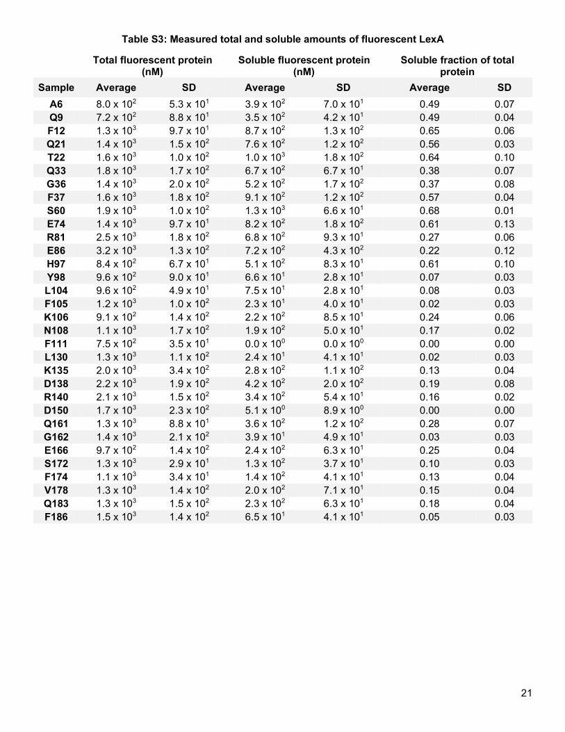
21
Table S3: Measured total and soluble amounts of fluorescent LexA
Total fluorescent protein (nM)
Soluble fluorescent protein (nM)
Soluble fraction of total protein
Sample Average SD Average SD Average SD A6 8.0 x 10² 5.3 x 101 3.9 x 10² 7.0 x 101 0.49 0.07 Q9 7.2 x 10² 8.8 x 101 3.5 x 10² 4.2 x 101 0.49 0.04 F12 1.3 x 10³ 9.7 x 101 8.7 x 10² 1.3 x 10² 0.65 0.06 Q21 1.4 x 10³ 1.5 x 10² 7.6 x 10² 1.2 x 10² 0.56 0.03 T22 1.6 x 10³ 1.0 x 10² 1.0 x 10³ 1.8 x 10² 0.64 0.10 Q33 1.8 x 10³ 1.7 x 10² 6.7 x 10² 6.7 x 101 0.38 0.07 G36 1.4 x 10³ 2.0 x 10² 5.2 x 10² 1.7 x 10² 0.37 0.08 F37 1.6 x 10³ 1.8 x 10² 9.1 x 10² 1.2 x 10² 0.57 0.04 S60 1.9 x 10³ 1.0 x 10² 1.3 x 10³ 6.6 x 101 0.68 0.01 E74 1.4 x 10³ 9.7 x 101 8.2 x 10² 1.8 x 10² 0.61 0.13 R81 2.5 x 10³ 1.8 x 10² 6.8 x 10² 9.3 x 101 0.27 0.06 E86 3.2 x 10³ 1.3 x 10² 7.2 x 10² 4.3 x 10² 0.22 0.12 H97 8.4 x 10² 6.7 x 101 5.1 x 10² 8.3 x 101 0.61 0.10 Y98 9.6 x 10² 9.0 x 101 6.6 x 101 2.8 x 101 0.07 0.03 L104 9.6 x 10² 4.9 x 101 7.5 x 101 2.8 x 101 0.08 0.03 F105 1.2 x 10³ 1.0 x 10² 2.3 x 101 4.0 x 101 0.02 0.03 K106 9.1 x 10² 1.4 x 10² 2.2 x 10² 8.5 x 101 0.24 0.06 N108 1.1 x 10³ 1.7 x 10² 1.9 x 10² 5.0 x 101 0.17 0.02 F111 7.5 x 10² 3.5 x 101 0.0 x 100 0.0 x 100 0.00 0.00 L130 1.3 x 10³ 1.1 x 10² 2.4 x 101 4.1 x 101 0.02 0.03 K135 2.0 x 10³ 3.4 x 10² 2.8 x 10² 1.1 x 10² 0.13 0.04 D138 2.2 x 10³ 1.9 x 10² 4.2 x 10² 2.0 x 10² 0.19 0.08 R140 2.1 x 10³ 1.5 x 10² 3.4 x 10² 5.4 x 101 0.16 0.02 D150 1.7 x 10³ 2.3 x 10² 5.1 x 100 8.9 x 100 0.00 0.00 Q161 1.3 x 10³ 8.8 x 101 3.6 x 10² 1.2 x 10² 0.28 0.07 G162 1.4 x 10³ 2.1 x 10² 3.9 x 101 4.9 x 101 0.03 0.03 E166 9.7 x 10² 1.4 x 10² 2.4 x 10² 6.3 x 101 0.25 0.04 S172 1.3 x 10³ 2.9 x 101 1.3 x 10² 3.7 x 101 0.10 0.03 F174 1.1 x 10³ 3.4 x 101 1.4 x 10² 4.1 x 101 0.13 0.04 V178 1.3 x 10³ 1.4 x 10² 2.0 x 10² 7.1 x 101 0.15 0.04 Q183 1.3 x 10³ 1.5 x 10² 2.3 x 10² 6.3 x 101 0.18 0.04 F186 1.5 x 10³ 1.4 x 10² 6.5 x 101 4.1 x 101 0.05 0.03
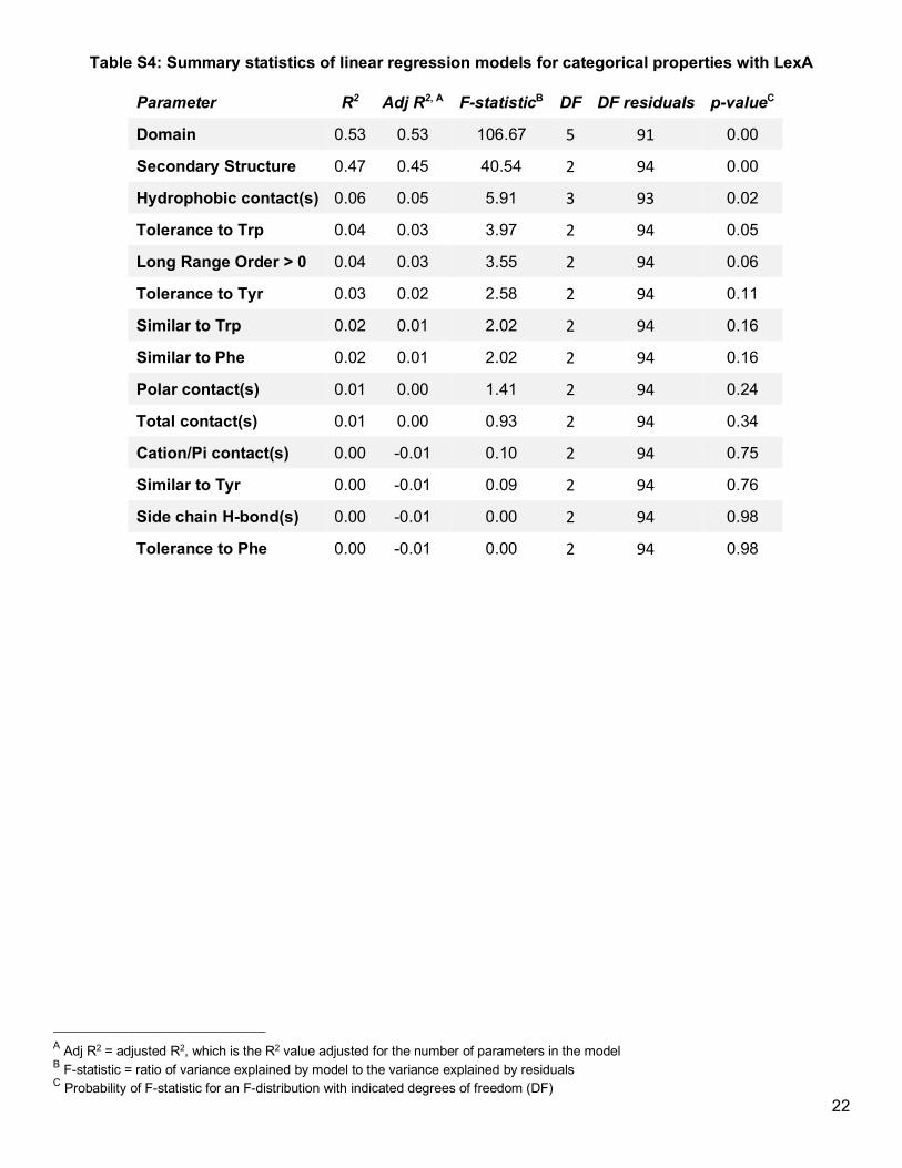
22
Table S4: Summary statistics of linear regression models for categorical properties with LexA
Parameter R2 Adj R2, A F-statisticB DF DF residuals p-valueC
Domain 0.53 0.53 106.67 5 91 0.00
Secondary Structure 0.47 0.45 40.54 2 94 0.00
Hydrophobic contact(s) 0.06 0.05 5.91 3 93 0.02
Tolerance to Trp 0.04 0.03 3.97 2 94 0.05
Long Range Order > 0 0.04 0.03 3.55 2 94 0.06
Tolerance to Tyr 0.03 0.02 2.58 2 94 0.11
Similar to Trp 0.02 0.01 2.02 2 94 0.16
Similar to Phe 0.02 0.01 2.02 2 94 0.16
Polar contact(s) 0.01 0.00 1.41 2 94 0.24
Total contact(s) 0.01 0.00 0.93 2 94 0.34
Cation/Pi contact(s) 0.00 -0.01 0.10 2 94 0.75
Similar to Tyr 0.00 -0.01 0.09 2 94 0.76
Side chain H-bond(s) 0.00 -0.01 0.00 2 94 0.98
Tolerance to Phe 0.00 -0.01 0.00 2 94 0.98
A Adj R2 = adjusted R2, which is the R2 value adjusted for the number of parameters in the model B F-statistic = ratio of variance explained by model to the variance explained by residuals C Probability of F-statistic for an F-distribution with indicated degrees of freedom (DF)
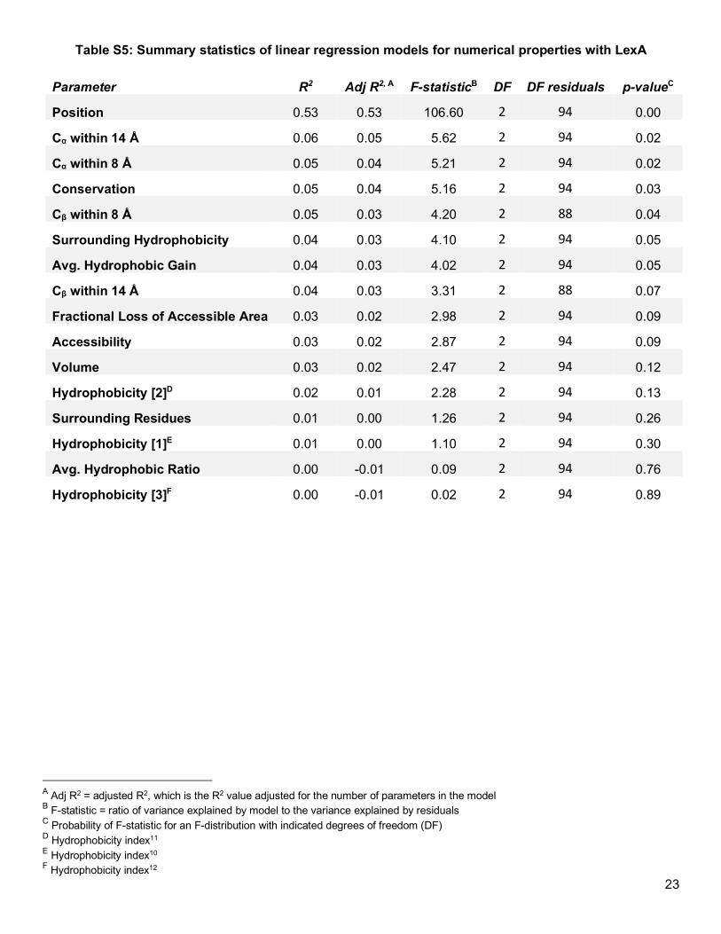
23
Table S5: Summary statistics of linear regression models for numerical properties with LexA
Parameter R2 Adj R2, A F-statisticB DF DF residuals p-valueC
Position 0.53 0.53 106.60 2 94 0.00
Cα within 14 Å 0.06 0.05 5.62 2 94 0.02
Cα within 8 Å 0.05 0.04 5.21 2 94 0.02
Conservation 0.05 0.04 5.16 2 94 0.03
Cβ within 8 Å 0.05 0.03 4.20 2 88 0.04
Surrounding Hydrophobicity 0.04 0.03 4.10 2 94 0.05
Avg. Hydrophobic Gain 0.04 0.03 4.02 2 94 0.05
Cβ within 14 Å 0.04 0.03 3.31 2 88 0.07
Fractional Loss of Accessible Area 0.03 0.02 2.98 2 94 0.09
Accessibility 0.03 0.02 2.87 2 94 0.09
Volume 0.03 0.02 2.47 2 94 0.12
Hydrophobicity [2]D 0.02 0.01 2.28 2 94 0.13
Surrounding Residues 0.01 0.00 1.26 2 94 0.26
Hydrophobicity [1]E 0.01 0.00 1.10 2 94 0.30
Avg. Hydrophobic Ratio 0.00 -0.01 0.09 2 94 0.76
Hydrophobicity [3]F 0.00 -0.01 0.02 2 94 0.89
A Adj R2 = adjusted R2, which is the R2 value adjusted for the number of parameters in the model B F-statistic = ratio of variance explained by model to the variance explained by residuals C Probability of F-statistic for an F-distribution with indicated degrees of freedom (DF) D Hydrophobicity index11 E Hydrophobicity index10 F Hydrophobicity index12
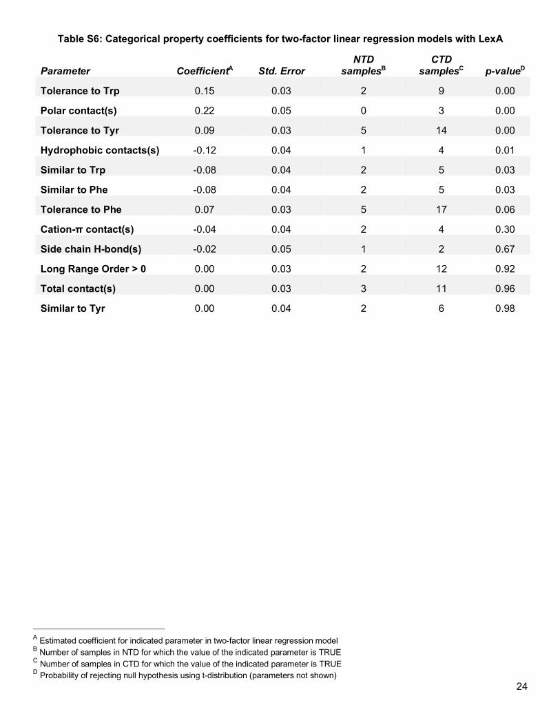
24
Table S6: Categorical property coefficients for two-factor linear regression models with LexA
Parameter CoefficientA Std. Error NTD
samplesB CTD
samplesC p-valueD
Tolerance to Trp 0.15 0.03 2 9 0.00
Polar contact(s) 0.22 0.05 0 3 0.00
Tolerance to Tyr 0.09 0.03 5 14 0.00
Hydrophobic contacts(s) -0.12 0.04 1 4 0.01
Similar to Trp -0.08 0.04 2 5 0.03
Similar to Phe -0.08 0.04 2 5 0.03
Tolerance to Phe 0.07 0.03 5 17 0.06
Cation-π contact(s) -0.04 0.04 2 4 0.30
Side chain H-bond(s) -0.02 0.05 1 2 0.67
Long Range Order > 0 0.00 0.03 2 12 0.92
Total contact(s) 0.00 0.03 3 11 0.96
Similar to Tyr 0.00 0.04 2 6 0.98
A Estimated coefficient for indicated parameter in two-factor linear regression model B Number of samples in NTD for which the value of the indicated parameter is TRUE C Number of samples in CTD for which the value of the indicated parameter is TRUE D Probability of rejecting null hypothesis using t-distribution (parameters not shown)
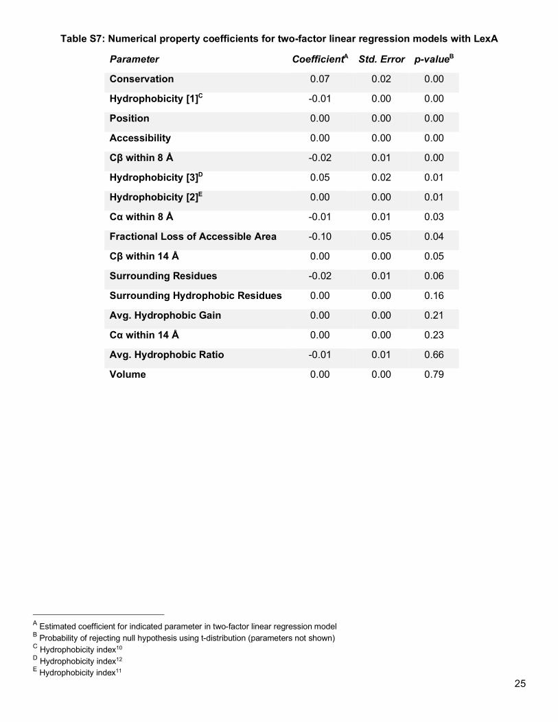
25
Table S7: Numerical property coefficients for two-factor linear regression models with LexA
Parameter CoefficientA Std. Error p-valueB
Conservation 0.07 0.02 0.00
Hydrophobicity [1]C -0.01 0.00 0.00
Position 0.00 0.00 0.00
Accessibility 0.00 0.00 0.00
Cβ within 8 Å -0.02 0.01 0.00
Hydrophobicity [3]D 0.05 0.02 0.01
Hydrophobicity [2]E 0.00 0.00 0.01
Cα within 8 Å -0.01 0.01 0.03
Fractional Loss of Accessible Area -0.10 0.05 0.04
Cβ within 14 Å 0.00 0.00 0.05
Surrounding Residues -0.02 0.01 0.06
Surrounding Hydrophobic Residues 0.00 0.00 0.16
Avg. Hydrophobic Gain 0.00 0.00 0.21
Cα within 14 Å 0.00 0.00 0.23
Avg. Hydrophobic Ratio -0.01 0.01 0.66
Volume 0.00 0.00 0.79
A Estimated coefficient for indicated parameter in two-factor linear regression model B Probability of rejecting null hypothesis using t-distribution (parameters not shown) C Hydrophobicity index10 D Hydrophobicity index12 E Hydrophobicity index11
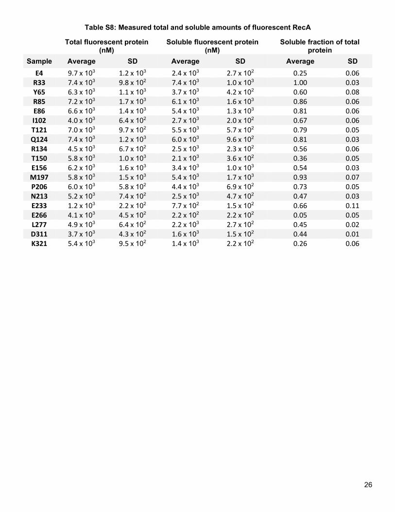
26
Table S8: Measured total and soluble amounts of fluorescent RecA
Total fluorescent protein (nM)
Soluble fluorescent protein (nM)
Soluble fraction of total protein
Sample Average SD Average SD Average SD E4 9.7 x 10³ 1.2 x 10³ 2.4 x 10³ 2.7 x 10² 0.25 0.06 R33 7.4 x 10³ 9.8 x 10² 7.4 x 10³ 1.0 x 10³ 1.00 0.03 Y65 6.3 x 10³ 1.1 x 10³ 3.7 x 10³ 4.2 x 10² 0.60 0.08 R85 7.2 x 10³ 1.7 x 10³ 6.1 x 10³ 1.6 x 10³ 0.86 0.06 E86 6.6 x 10³ 1.4 x 10³ 5.4 x 10³ 1.3 x 10³ 0.81 0.06 I102 4.0 x 10³ 6.4 x 10² 2.7 x 10³ 2.0 x 10² 0.67 0.06 T121 7.0 x 10³ 9.7 x 10² 5.5 x 10³ 5.7 x 10² 0.79 0.05 Q124 7.4 x 10³ 1.2 x 10³ 6.0 x 10³ 9.6 x 10² 0.81 0.03 R134 4.5 x 10³ 6.7 x 10² 2.5 x 10³ 2.3 x 10² 0.56 0.06 T150 5.8 x 10³ 1.0 x 10³ 2.1 x 10³ 3.6 x 10² 0.36 0.05 E156 6.2 x 10³ 1.6 x 10³ 3.4 x 10³ 1.0 x 10³ 0.54 0.03 M197 5.8 x 10³ 1.5 x 10³ 5.4 x 10³ 1.7 x 10³ 0.93 0.07 P206 6.0 x 10³ 5.8 x 10² 4.4 x 10³ 6.9 x 10² 0.73 0.05 N213 5.2 x 10³ 7.4 x 10² 2.5 x 10³ 4.7 x 10² 0.47 0.03 E233 1.2 x 10³ 2.2 x 10² 7.7 x 10² 1.5 x 10² 0.66 0.11 E266 4.1 x 10³ 4.5 x 10² 2.2 x 10² 2.2 x 10² 0.05 0.05 L277 4.9 x 10³ 6.4 x 10² 2.2 x 10³ 2.7 x 10² 0.45 0.02 D311 3.7 x 10³ 4.3 x 10² 1.6 x 10³ 1.5 x 10² 0.44 0.01 K321 5.4 x 10³ 9.5 x 10² 1.4 x 10³ 2.2 x 10² 0.26 0.06
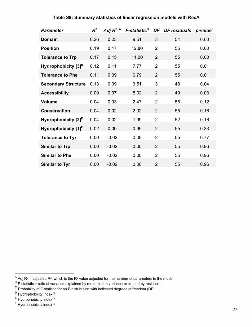
27
Table S9: Summary statistics of linear regression models with RecA
Parameter R2 Adj R2, A F-statisticB DF DF residuals p-valueC
Domain 0.26 0.23 9.51 3 54 0.00
Position 0.19 0.17 12.80 2 55 0.00
Tolerance to Trp 0.17 0.15 11.00 2 55 0.00
Hydrophobicity [3]D 0.12 0.11 7.77 2 55 0.01
Tolerance to Phe 0.11 0.09 6.79 2 55 0.01
Secondary Structure 0.13 0.09 3.51 3 48 0.04
Accessibility 0.09 0.07 5.02 2 49 0.03
Volume 0.04 0.03 2.47 2 55 0.12
Conservation 0.04 0.02 2.02 2 55 0.16
Hydrophobicity [2]E 0.04 0.02 1.99 2 52 0.16
Hydrophobicity [1]F 0.02 0.00 0.99 2 55 0.33
Tolerance to Tyr 0.00 -0.02 0.09 2 55 0.77
Similar to Trp 0.00 -0.02 0.00 2 55 0.96
Similar to Phe 0.00 -0.02 0.00 2 55 0.96
Similar to Tyr 0.00 -0.02 0.00 2 55 0.96
A Adj R2 = adjusted R2, which is the R2 value adjusted for the number of parameters in the model B F-statistic = ratio of variance explained by model to the variance explained by residuals C Probability of F-statistic for an F-distribution with indicated degrees of freedom (DF) D Hydrophobicity index12 E Hydrophobicity index11 F Hydrophobicity index10
28
Supplemental References (1) Sungwienwong, I., Hostetler, Z. M., Blizzard, R. J., Porter, J. J., Driggers, C. M., Mbengi, L. Z., Villegas, J.
A., Speight, L. C., Saven, J. G., Perona, J. J., Kohli, R. M., Mehl, R. A., and Petersson, E. J. (2017) Improving
target amino acid selectivity in a permissive aminoacyl tRNA synthetase through counter-selection. Org.
Biomol. Chem. 15, 3603–3610.
(2) Mo, C. Y., Culyba, M. J., Selwood, T., Kubiak, J. M., Hostetler, Z. M., Jurewicz, A. J., Keller, P. M., Pope, A.
J., Quinn, A., Schneck, J., Widdowson, K. L., and Kohli, R. M. (2018) Inhibitors of LexA Autoproteolysis and
the Bacterial SOS Response Discovered by an Academic-Industry Partnership. ACS Infect. Dis. 4, 349–359.
(3) Speight, L. C., Muthusamy, A. K., Goldberg, J. M., Warner, J. B., Wissner, R. F., Willi, T. S., Woodman, B.
F., Mehl, R. A., and Petersson, E. J. (2013) Efficient synthesis and in vivo incorporation of acridon-2-ylalanine,
a fluorescent amino acid for lifetime and Förster resonance energy transfer/luminescence resonance energy
transfer studies. J. Am. Chem. Soc. 135, 18806–18814.
(4) Studier, F. W. (2014) Stable expression clones and auto-induction for protein production in E. coli. Methods
Mol. Biol. 1091, 17–32.
(5) Shibata, T., Osber, L., and Radding, C. M. (1983) Purification of recA protein from Escherichia coli.
Methods Enzymol. 100, 197–209.
(6) Henikoff, S., and Henikoff, J. G. (1992) Amino acid substitution matrices from protein blocks. Proc. Natl.
Acad. Sci. U. S. A. 89, 10915–10919.
(7) Zamyatnin, A. A. (1972) Protein volume in solution. Prog. Biophys. Mol. Biol. 24, 107–123.
(8) Tien, M. Z., Meyer, A. G., Sydykova, D. K., Spielman, S. J., and Wilke, C. O. (2013) Maximum allowed
solvent accessibilites of residues in proteins. PLoS One (Porollo, A., Ed.) 8, e80635.
(9) Heinig, M., and Frishman, D. (2004) STRIDE: a web server for secondary structure assignment from known
atomic coordinates of proteins. Nucleic Acids Res. 32, W500–W502.
(10) Wolfenden, R. (2007) Experimental measures of amino acid hydrophobicity and the topology of
transmembrane and globular proteins. J. Gen. Physiol. 129, 357–362.
(11) Monera, O. D., Sereda, T. J., Zhou, N. E., Kay, C. M., and Hodges, R. S. (1995) Relationship of sidechain
hydrophobicity and alpha-helical propensity on the stability of the single-stranded amphipathic alpha-helix. J.
Pept. Sci. 1, 319–329.
(12) Wimley, W. C., and White, S. H. (1996) Experimentally determined hydrophobicity scale for proteins at
membrane interfaces. Nat. Struct. Biol. 3, 842–848.
(13) Sim, N.-L., Kumar, P., Hu, J., Henikoff, S., Schneider, G., and Ng, P. C. (2012) SIFT web server:
predicting effects of amino acid substitutions on proteins. Nucleic Acids Res. 40, W452–W457.
(14) Celniker, G., Nimrod, G., Ashkenazy, H., Glaser, F., Martz, E., Mayrose, I., Pupko, T., and Ben-Tal, N.
(2013) ConSurf: Using Evolutionary Data to Raise Testable Hypotheses about Protein Function. Isr. J. Chem.
53, 199–206.
(15) Goldenberg, O., Erez, E., Nimrod, G., and Ben-Tal, N. (2009) The ConSurf-DB: pre-calculated
evolutionary conservation profiles of protein structures. Nucleic Acids Res. 37, D323–D327.
29
(16) Nagarajan, R., Archana, A., Thangakani, A. M., Jemimah, S., Velmurugan, D., and Gromiha, M. M. (2016)
PDBparam: Online Resource for Computing Structural Parameters of Proteins. Bioinform. Biol. Insights 10,
73–80.
(17) R core team. (2017) R: A language and environment for statistical computing. R Found. Stat. Comput.
Vienna, Austria.
(18) Wickham, H. (2016) tidyverse: Easily Install and Load “Tidyverse” Packages. R Packag. version 1.0.0.
(19) Schneider, C. A., Rasband, W. S., and Eliceiri, K. W. (2012) NIH Image to ImageJ: 25 years of image
analysis. Nat. Methods 9, 671–675.
(20) Drew, K., Renfrew, P. D., Craven, T. W., Butterfoss, G. L., Chou, F.-C., Lyskov, S., Bullock, B. N.,
Watkins, A., Labonte, J. W., Pacella, M., Kilambi, K. P., Leaver-Fay, A., Kuhlman, B., Gray, J. J., Bradley, P.,
Kirshenbaum, K., Arora, P. S., Das, R., and Bonneau, R. (2013) Adding diverse noncanonical backbones to
rosetta: enabling peptidomimetic design. PLoS One 8, e67051.
(21) Huang, P.-S., Ban, Y.-E. A., Richter, F., Andre, I., Vernon, R., Schief, W. R., and Baker, D. (2011)
RosettaRemodel: a generalized framework for flexible backbone protein design. PLoS One 6, e24109.