https://www.halvorsen.blog
https://www.halvorsen.blog/documents/automation/
SystemIdentification andEstimationinLabVIEW
Hans-PetterHalvorsen
SystemIdentificationandEstimationinLabVIEW
Hans-PetterHalvorsen
Copyright©2017
E-Mail:[email protected]
Web:https://www.halvorsen.blog
https://www.halvorsen.blog
i
PrefaceThisTutorialwillgothroughthebasicprinciplesofSystemidentificationandEstimationandhowtoimplementthesetechniquesinLabVIEWandLabVIEWMathScript.
LabVIEWisagraphicalprogramminglanguagecreatedbyNationalInstruments,whileLabVIEWMathScriptisanadd-ontoLabVIEW.LabVIEWMathScripthassimilarsyntaxas,e.g.,MATLAB.LabVIEWMathScriptmaybeusedasaseparatepart(andcanbeconsideredasaminiatureversionofMATLAB)orbeintegratedintothegraphicalLabVIEWcodeusingtheMathScriptNode.
Thefollowingmethodswillbediscussed:
StateEstimation:
• KalmanFilter• Observers
ParameterEstimation:
• LeastSquareMethod(LS)
SystemIdentification
• Sub-spacemethods/Black-Boxmethods• PolynomialModelEstimation:ARX/ARMAXmodelEstimation
Software
YouneedthefollowingsoftwareinthisTutorial:
• LabVIEW• LabVIEWControlDesignandSimulationModule• LabVIEWMathScriptRTModule(LabVIEWMathScript)
“LabVIEWControlDesignandSimulationModule”hasfunctionalityforcreatingKalmanFiltersandObservers,butitalsohasfunctionalityforSystemidentification.

ii
TableofContentsPreface.......................................................................................................................................i
TableofContents......................................................................................................................ii
1 IntroductiontoLabVIEWandMathScript.........................................................................5
1.1 LabVIEW....................................................................................................................5
1.2 LabVIEWMathScript..................................................................................................6
2 LabVIEWControlandSimulationModule.........................................................................9
3 ModelCreationinLabVIEW............................................................................................11
3.1 State-spaceModels.................................................................................................12
3.2 Transferfunctions...................................................................................................15
3.2.1 commonlyusedtransferfunctions..................................................................17
4 IntroductiontoSystemIdentificationandEstimation....................................................24
5 StateEstimationwithKalmanFilter................................................................................26
5.1 State-Spacemodel...................................................................................................27
5.2 Observability...........................................................................................................29
5.3 IntroductiontotheStateEstimator........................................................................30
5.4 StateEstimation......................................................................................................36
5.5 LabVIEWKalmanFilterImplementations................................................................38
6 CreateyourownKalmanFilterfromScratch..................................................................44
6.1 TheKalmanFilterAlgorithm....................................................................................44
6.2 Examples.................................................................................................................45
7 OverviewofKalmanFilterVIs.........................................................................................49
7.1 ControlDesignpalette.............................................................................................49
7.1.1 StateFeedbackDesignsubpalette..................................................................49
7.1.2 Implementationsubpalette.............................................................................50
iii TableofContents
Tutorial:SystemIdentificationandEstimationinLabVIEW
7.2 Simulationpalette...................................................................................................51
7.2.1 Estimationsubpalette.....................................................................................51
8 StateEstimationwithObserversinLabVIEW..................................................................54
8.1 State-Spacemodel...................................................................................................54
8.2 Eigenvalues..............................................................................................................56
8.3 ObserverGain..........................................................................................................57
8.4 Observability...........................................................................................................58
8.5 Examples.................................................................................................................59
9 OverviewofObserverfunctions......................................................................................64
9.1 ControlDesignpalette.............................................................................................64
9.1.1 StateFeedbackDesignsubpalette..................................................................64
9.1.2 Implementationsubpalette.............................................................................65
9.2 Simulationpalette...................................................................................................66
9.2.1 Estimationsubpalette.....................................................................................66
10 SystemIdentificationinLabVIEW................................................................................69
10.1 ParameterEstimationwithLeastSquareMethod(LS)...........................................70
10.2 SystemIdentificationusingSub-spacemethods/Black-Boxmethods.....................73
10.3 SystemIdentificationusingPolynomialModelEstimation:ARX/ARMAXmodelEstimation...........................................................................................................................74
10.4 GeneratemodelData..............................................................................................75
10.4.1 Excitationsignals.............................................................................................77
11 OverviewofSystemIdentificationfunctions..............................................................80
12 SystemIdentificationExample....................................................................................85
4
PartI:Introduction
5
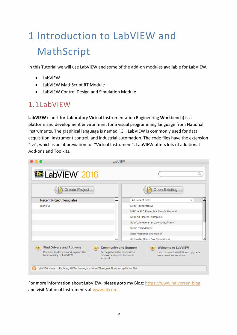
1 IntroductiontoLabVIEWandMathScript
InthisTutorialwewilluseLabVIEWandsomeoftheadd-onmodulesavailableforLabVIEW.
• LabVIEW• LabVIEWMathScriptRTModule• LabVIEWControlDesignandSimulationModule
1.1 LabVIEWLabVIEW(shortforLaboratoryVirtualInstrumentationEngineeringWorkbench)isaplatformanddevelopmentenvironmentforavisualprogramminglanguagefromNationalInstruments.Thegraphicallanguageisnamed"G".LabVIEWiscommonlyusedfordataacquisition,instrumentcontrol,andindustrialautomation.Thecodefileshavetheextension“.vi”,whichisanabbreviationfor“VirtualInstrument”.LabVIEWofferslotsofadditionalAdd-onsandToolkits.
FormoreinformationaboutLabVIEW,pleasegotomyBlog:https://www.halvorsen.blog andvisitNationalInstrumentsatwww.ni.com.
6 IntroductiontoLabVIEWandMathScript
Tutorial:SystemIdentificationandEstimationinLabVIEW
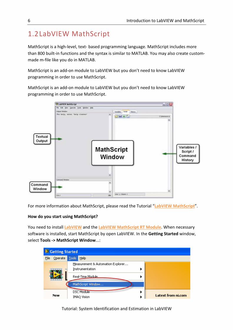
1.2 LabVIEWMathScriptMathScriptisahigh-level,text-basedprogramminglanguage.MathScriptincludesmorethan800built-infunctionsandthesyntaxissimilartoMATLAB.Youmayalsocreatecustom-madem-filelikeyoudoinMATLAB.
MathScriptisanadd-onmoduletoLabVIEWbutyoudon’tneedtoknowLabVIEWprogramminginordertouseMathScript.
MathScriptisanadd-onmoduletoLabVIEWbutyoudon’tneedtoknowLabVIEWprogramminginordertouseMathScript.
FormoreinformationaboutMathScript,pleasereadtheTutorial“LabVIEWMathScript”.
HowdoyoustartusingMathScript?
YouneedtoinstallLabVIEWandtheLabVIEWMathScriptRTModule.Whennecessarysoftwareisinstalled,startMathScriptbyopenLabVIEW.IntheGettingStartedwindow,selectTools->MathScriptWindow...:
7 IntroductiontoLabVIEWandMathScript
Tutorial:SystemIdentificationandEstimationinLabVIEW
FormoreinformationaboutMathScript,pleasereadtheTutorial“LabVIEWMathScript”.
MathScriptNode:
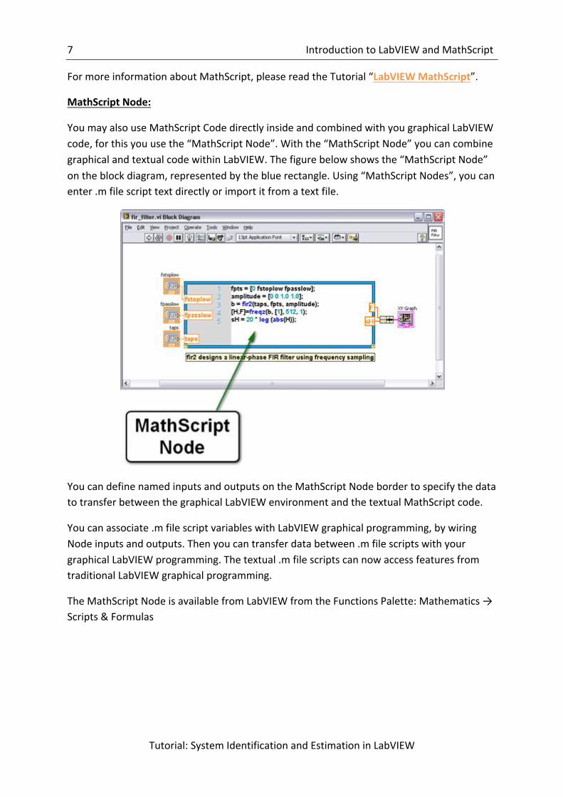
YoumayalsouseMathScriptCodedirectlyinsideandcombinedwithyougraphicalLabVIEWcode,forthisyouusethe“MathScriptNode”.Withthe“MathScriptNode”youcancombinegraphicalandtextualcodewithinLabVIEW.Thefigurebelowshowsthe“MathScriptNode”ontheblockdiagram,representedbythebluerectangle.Using“MathScriptNodes”,youcanenter.mfilescripttextdirectlyorimportitfromatextfile.
YoucandefinenamedinputsandoutputsontheMathScriptNodebordertospecifythedatatotransferbetweenthegraphicalLabVIEWenvironmentandthetextualMathScriptcode.
Youcanassociate.mfilescriptvariableswithLabVIEWgraphicalprogramming,bywiringNodeinputsandoutputs.Thenyoucantransferdatabetween.mfilescriptswithyourgraphicalLabVIEWprogramming.Thetextual.mfilescriptscannowaccessfeaturesfromtraditionalLabVIEWgraphicalprogramming.
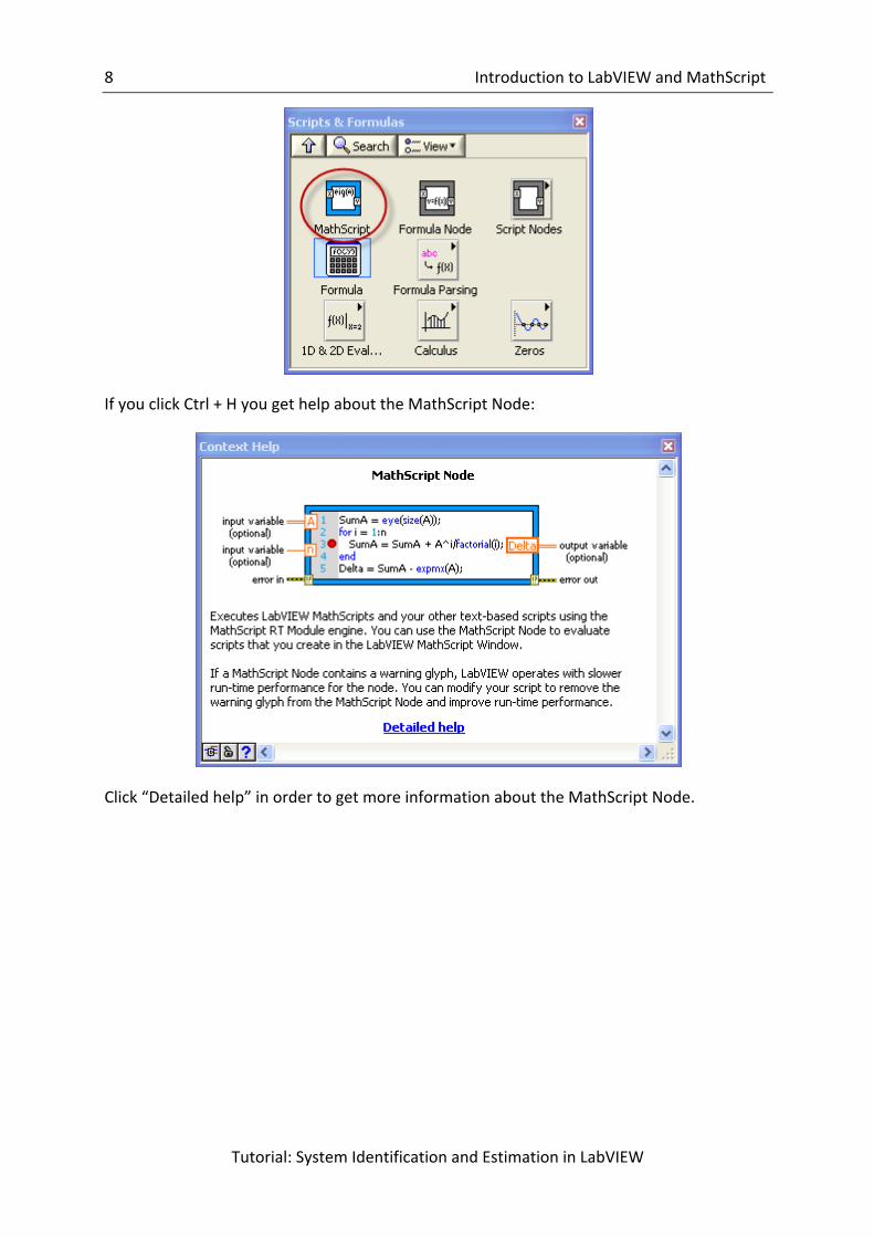
TheMathScriptNodeisavailablefromLabVIEWfromtheFunctionsPalette:Mathematics→Scripts&Formulas
8 IntroductiontoLabVIEWandMathScript
Tutorial:SystemIdentificationandEstimationinLabVIEW
IfyouclickCtrl+HyougethelpabouttheMathScriptNode:
Click“Detailedhelp”inordertogetmoreinformationabouttheMathScriptNode.
9
2 LabVIEWControlandSimulationModule
LabVIEWhasseveraladditionalmodulesandToolkitsforControlandSimulationpurposes,e.g.,“LabVIEWControlDesignandSimulationModule”,“LabVIEWPIDandFuzzyLogicToolkit”,“LabVIEWSystemIdentificationToolkit”and“LabVIEWSimulationInterfaceToolkit”.LabVIEWMathScriptisalsousefulforControlDesignandSimulation.
• LabVIEWControlDesignandSimulationModule• LabVIEWPIDandFuzzyLogicToolkit• LabVIEWSystemIdentificationToolkit• LabVIEWSimulationInterfaceToolkit
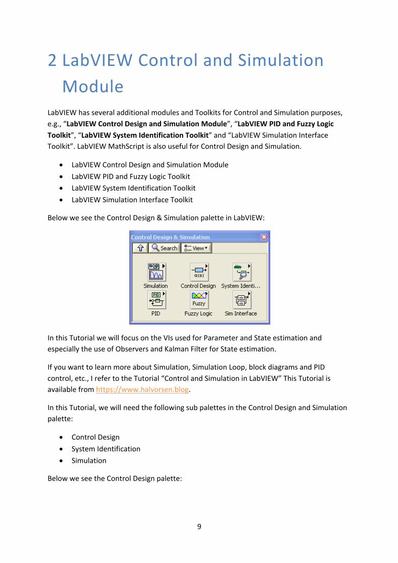
BelowweseetheControlDesign&SimulationpaletteinLabVIEW:
InthisTutorialwewillfocusontheVIsusedforParameterandStateestimationandespeciallytheuseofObserversandKalmanFilterforStateestimation.
IfyouwanttolearnmoreaboutSimulation,SimulationLoop,blockdiagramsandPIDcontrol,etc.,IrefertotheTutorial“ControlandSimulationinLabVIEW”ThisTutorialisavailablefromhttps://www.halvorsen.blog.
InthisTutorial,wewillneedthefollowingsubpalettesintheControlDesignandSimulationpalette:
• ControlDesign• SystemIdentification• Simulation
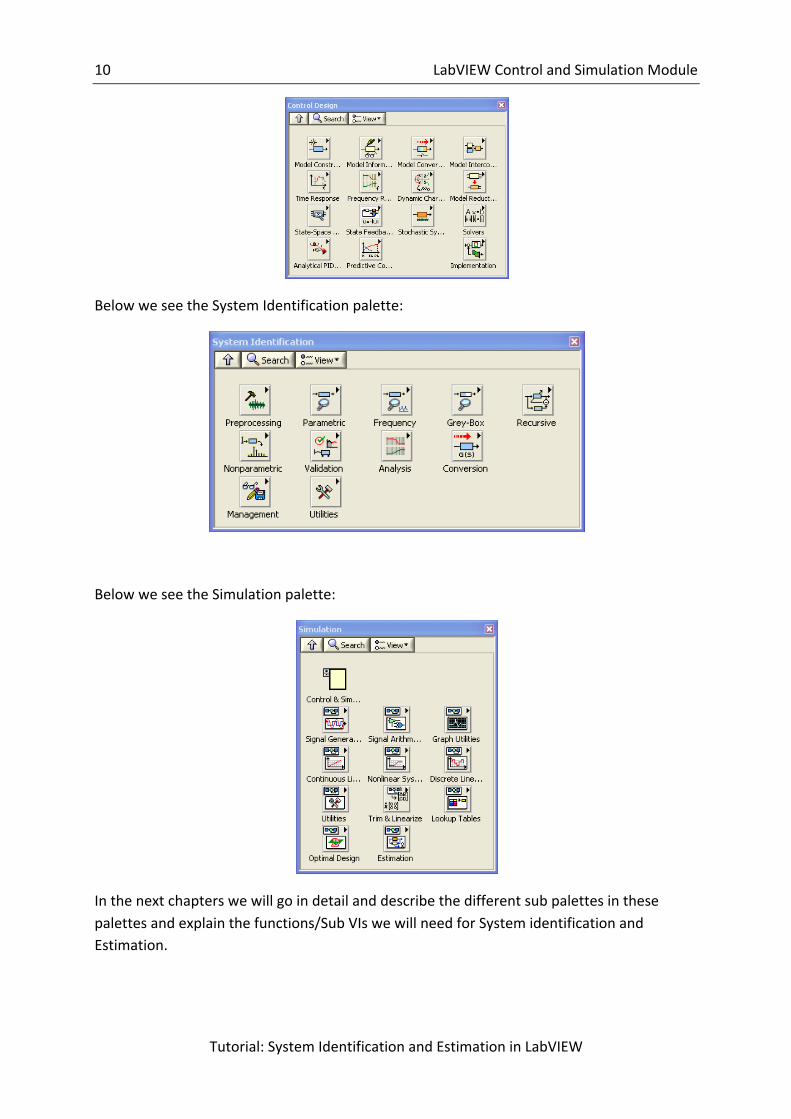
BelowweseetheControlDesignpalette:
10 LabVIEWControlandSimulationModule
Tutorial:SystemIdentificationandEstimationinLabVIEW
BelowweseetheSystemIdentificationpalette:
BelowweseetheSimulationpalette:
Inthenextchapterswewillgoindetailanddescribethedifferentsubpalettesinthesepalettesandexplainthefunctions/SubVIswewillneedforSystemidentificationandEstimation.

11
3 ModelCreationinLabVIEWWhenyouhavefoundthemathematicalmodelforyoursystem,thefirststepistodefine/orcreateyourmodelinLabVIEW.YourmodelcanbeaTransferfunctionoraState-spacemodel.
InLabVIEWandthe“LabVIEWControlDesignandSimulationModule”youcancreatedifferentmodels,suchasState-spacemodelsandtransferfunctions,etc.
IntheControlDesignpalette,wehaveseveralsubpalettesthatdealswithmodels,theseare:
• ModelConstruction• ModelInformation• ModelConversion• ModelInterconnection
BelowwegothroughthedifferentsubpalettesandthemostusedVIsinthesepalettes.
“ModelConstruction”Subpalette:
InthispalettewehaveVIsforcreatingstate-spacemodelsandtransferfunctions.

12 ModelCreationinLabVIEW
Tutorial:SystemIdentificationandEstimationinLabVIEW
→UsetheModelConstructionVIstocreatelinearsystemmodelsandmodifythepropertiesofasystemmodel.YoualsocanusetheModelConstructionVIstosaveasystemmodeltoafile,readasystemmodelfromafile,orobtainavisualrepresentationofamodel.
SomeofthemostusedVIswouldbe:
CDConstructState-SpaceModel.vi
CDConstructTransferFunctionModel.vi
TheseVIsandsomeothersareexplainedbelow.
3.1 State-spaceModelsGiventhefollowingState-spacemodel:
𝑥 = 𝐴𝑥 + 𝐵𝑢
𝑦 = 𝐶𝑥 + 𝐷𝑢
InLabVIEWweusethe“CDConstructState-SpaceModel.vi”tocreateaState-spacemodel:
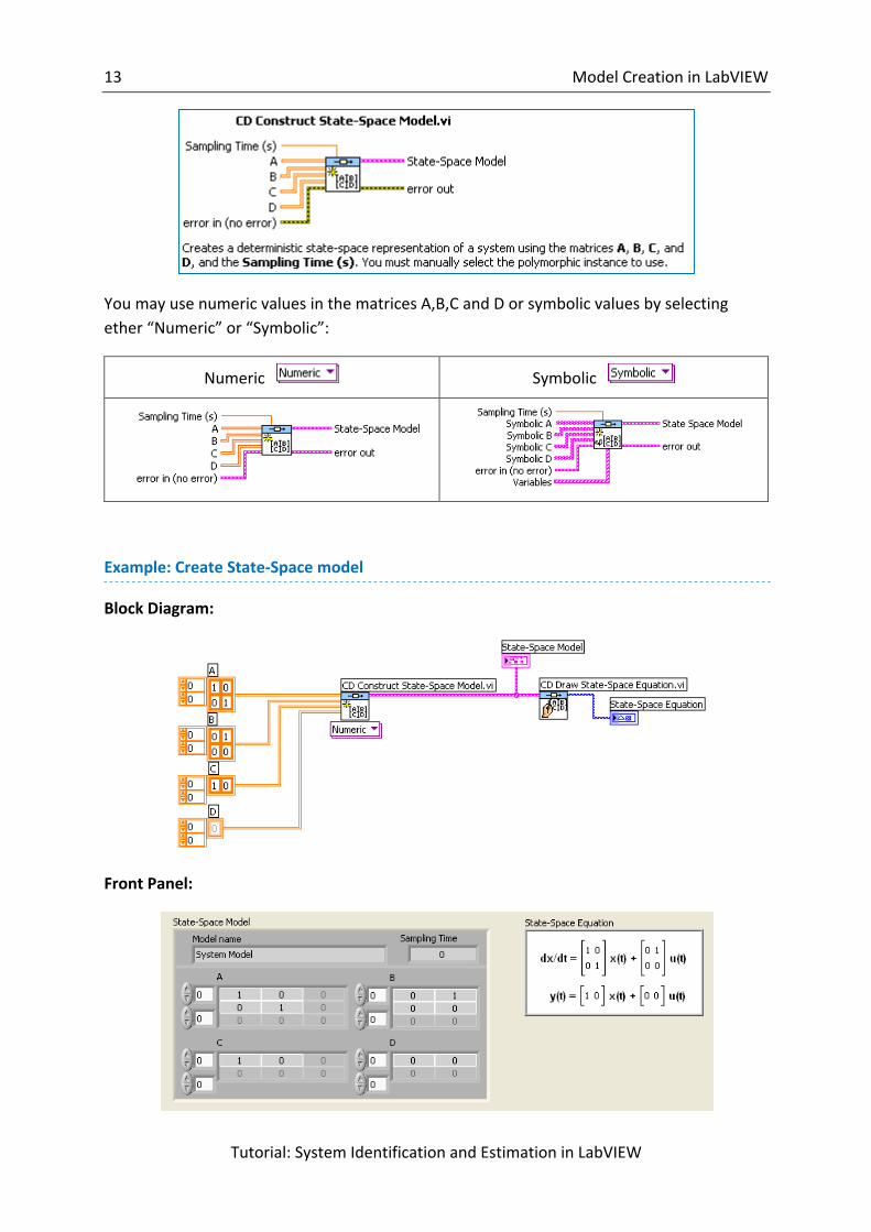
13 ModelCreationinLabVIEW
Tutorial:SystemIdentificationandEstimationinLabVIEW
YoumayusenumericvaluesinthematricesA,B,CandDorsymbolicvaluesbyselectingether“Numeric”or“Symbolic”:
Numeric Symbolic
Example:CreateState-Spacemodel
BlockDiagram:
FrontPanel:
14 ModelCreationinLabVIEW
Tutorial:SystemIdentificationandEstimationinLabVIEW
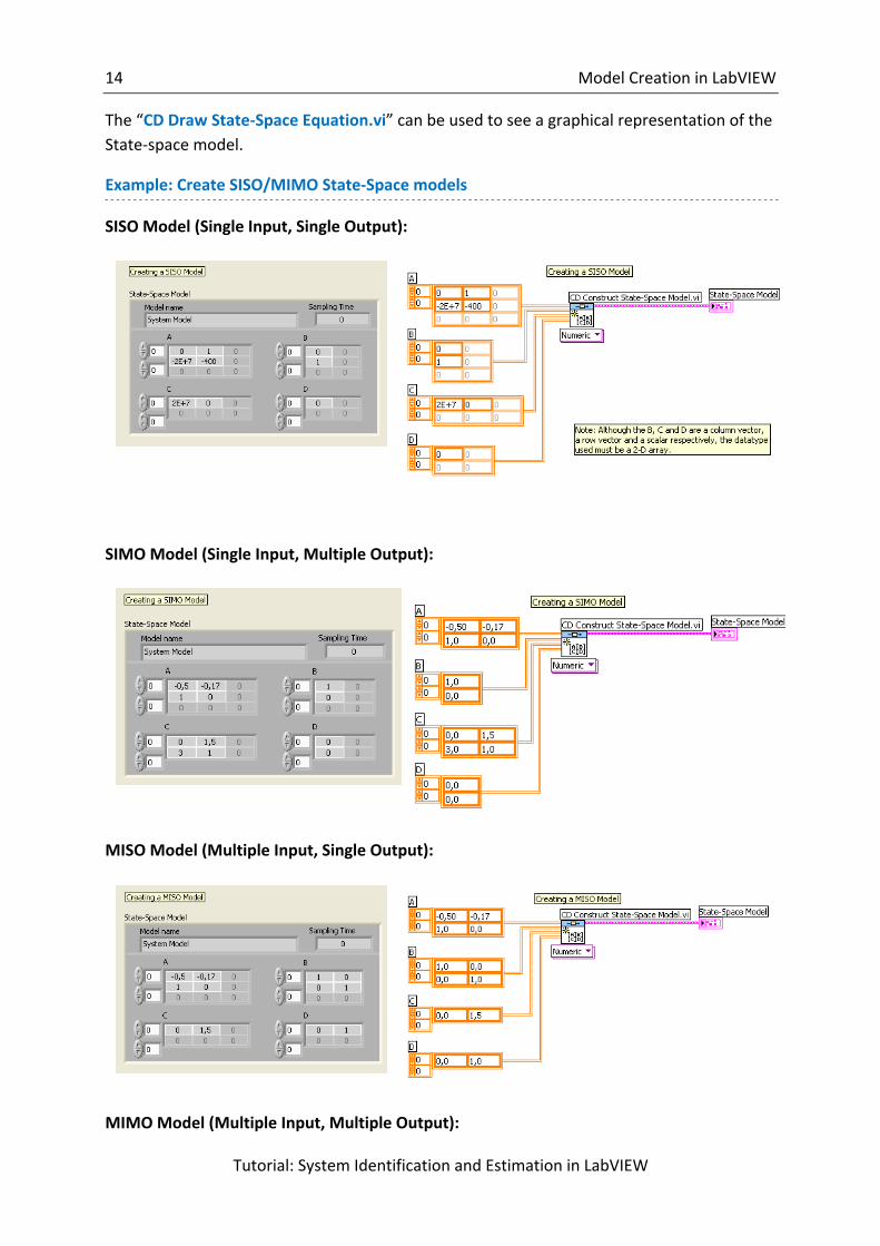
The“CDDrawState-SpaceEquation.vi”canbeusedtoseeagraphicalrepresentationoftheState-spacemodel.
Example:CreateSISO/MIMOState-Spacemodels
SISOModel(SingleInput,SingleOutput):
SIMOModel(SingleInput,MultipleOutput):
MISOModel(MultipleInput,SingleOutput):
MIMOModel(MultipleInput,MultipleOutput):
15 ModelCreationinLabVIEW
Tutorial:SystemIdentificationandEstimationinLabVIEW
[EndofExample]
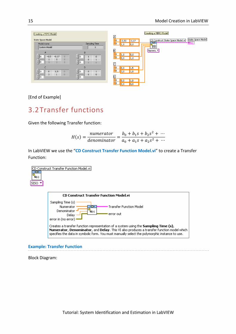
3.2 TransferfunctionsGiventhefollowingTransferfunction:
𝐻 𝑠 =𝑛𝑢𝑚𝑒𝑟𝑎𝑡𝑜𝑟𝑑𝑒𝑛𝑜𝑚𝑖𝑛𝑎𝑡𝑜𝑟
=𝑏6 + 𝑏7𝑠 + 𝑏8𝑠8 +⋯𝑎6 + 𝑎7𝑠 + 𝑎8𝑠8 +⋯
InLabVIEWweusethe“CDConstructTransferFunctionModel.vi”tocreateaTransferFunction:
Example:TransferFunction
BlockDiagram:
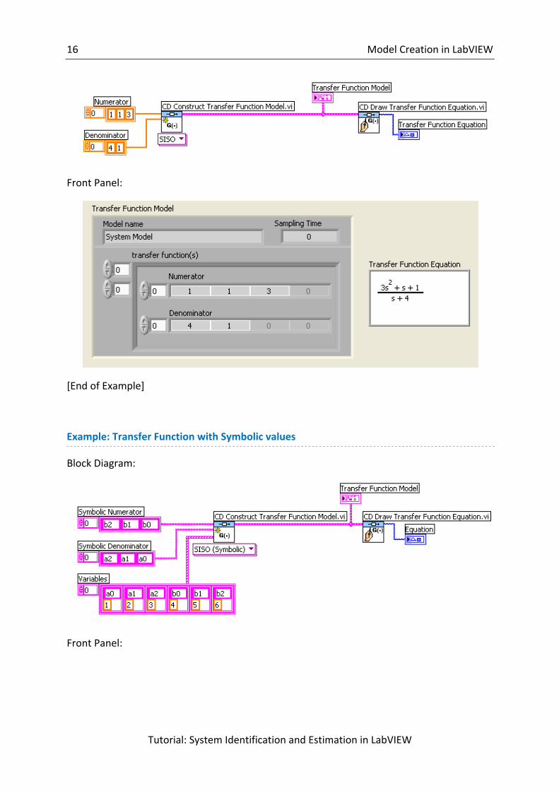
16 ModelCreationinLabVIEW
Tutorial:SystemIdentificationandEstimationinLabVIEW
FrontPanel:
[EndofExample]
Example:TransferFunctionwithSymbolicvalues
BlockDiagram:
FrontPanel:
17 ModelCreationinLabVIEW
Tutorial:SystemIdentificationandEstimationinLabVIEW
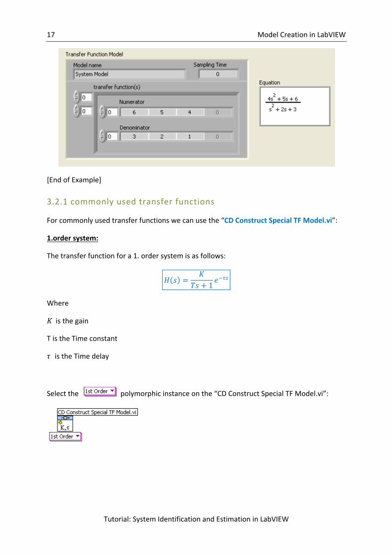
[EndofExample]
3.2.1 commonlyusedtransferfunctions
Forcommonlyusedtransferfunctionswecanusethe“CDConstructSpecialTFModel.vi”:
1.ordersystem:
Thetransferfunctionfora1.ordersystemisasfollows:
𝐻 𝑠 =𝐾
𝑇𝑠 + 1𝑒>?@
Where
𝐾 isthegain
TistheTimeconstant
𝜏 istheTimedelay
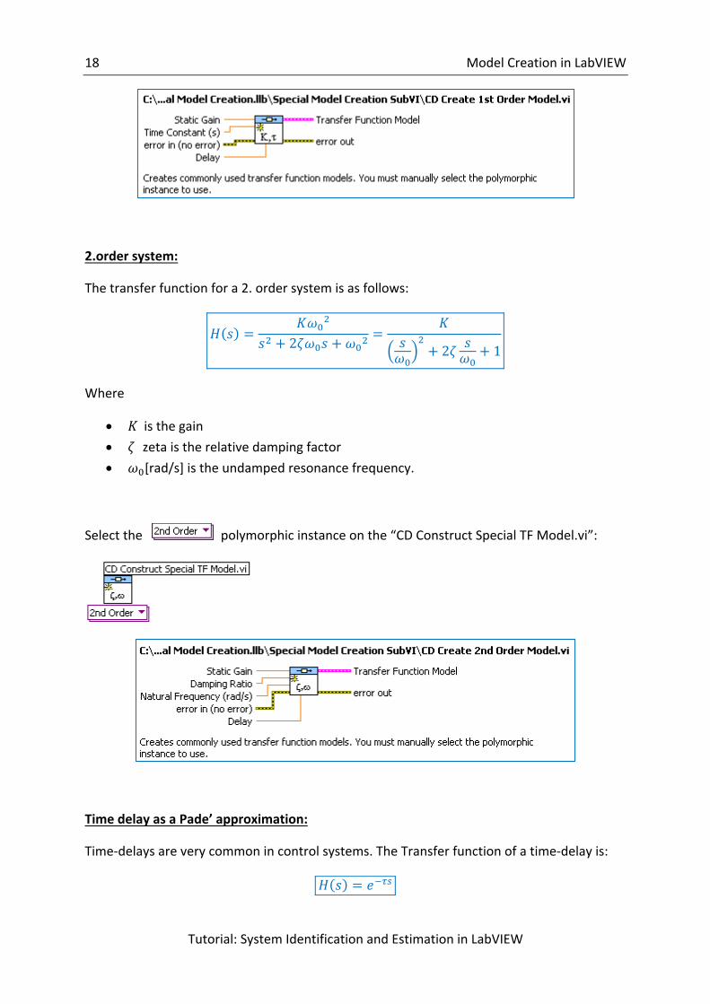
Selectthe polymorphicinstanceonthe“CDConstructSpecialTFModel.vi”:
18 ModelCreationinLabVIEW
Tutorial:SystemIdentificationandEstimationinLabVIEW
2.ordersystem:
Thetransferfunctionfora2.ordersystemisasfollows:
𝐻 𝑠 =𝐾𝜔68
𝑠8 + 2𝜁𝜔6𝑠 + 𝜔68=
𝐾𝑠𝜔6
8+ 2𝜁 𝑠
𝜔6+ 1
Where
• 𝐾 isthegain• 𝜁 zetaistherelativedampingfactor• 𝜔6[rad/s]istheundampedresonancefrequency.
Selectthe polymorphicinstanceonthe“CDConstructSpecialTFModel.vi”:
TimedelayasaPade’approximation:
Time-delaysareverycommonincontrolsystems.TheTransferfunctionofatime-delayis:
𝐻 𝑠 = 𝑒>?@
19 ModelCreationinLabVIEW
Tutorial:SystemIdentificationandEstimationinLabVIEW
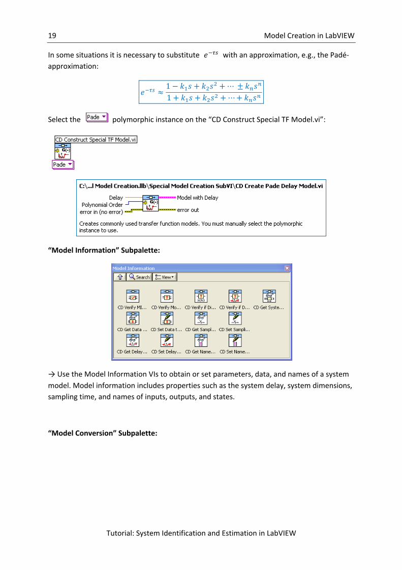
Insomesituationsitisnecessarytosubstitute 𝑒>?@ withanapproximation,e.g.,thePadé-approximation:
𝑒>?@ ≈1 − 𝑘7𝑠 + 𝑘8𝑠8 + ⋯± 𝑘I𝑠I
1 + 𝑘7𝑠 + 𝑘8𝑠8 + ⋯+ 𝑘I𝑠I
Selectthe polymorphicinstanceonthe“CDConstructSpecialTFModel.vi”:
“ModelInformation”Subpalette:
→UsetheModelInformationVIstoobtainorsetparameters,data,andnamesofasystemmodel.Modelinformationincludespropertiessuchasthesystemdelay,systemdimensions,samplingtime,andnamesofinputs,outputs,andstates.
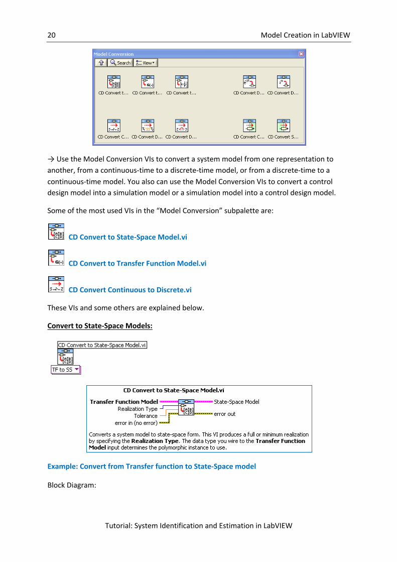
“ModelConversion”Subpalette:
20 ModelCreationinLabVIEW
Tutorial:SystemIdentificationandEstimationinLabVIEW
→UsetheModelConversionVIstoconvertasystemmodelfromonerepresentationtoanother,fromacontinuous-timetoadiscrete-timemodel,orfromadiscrete-timetoacontinuous-timemodel.YoualsocanusetheModelConversionVIstoconvertacontroldesignmodelintoasimulationmodelorasimulationmodelintoacontroldesignmodel.
SomeofthemostusedVIsinthe“ModelConversion”subpaletteare:
CDConverttoState-SpaceModel.vi
CDConverttoTransferFunctionModel.vi
CDConvertContinuoustoDiscrete.vi
TheseVIsandsomeothersareexplainedbelow.
ConverttoState-SpaceModels:
Example:ConvertfromTransferfunctiontoState-Spacemodel
BlockDiagram:

21 ModelCreationinLabVIEW
Tutorial:SystemIdentificationandEstimationinLabVIEW
FrontPanel:
[EndofExample]
ConverttoTransferFunctions:
Example:ConvertfromState-SpacemodeltoTransferFunction
BlockDiagram:
FrontPanel:

22 ModelCreationinLabVIEW
Tutorial:SystemIdentificationandEstimationinLabVIEW
[EndofExample]
ConvertContinuoustoDiscreteModel:
Example:ConvertfromContinuousState-SpacemodeltoDiscreteState-Spacemodel
BlockDiagram:
FrontPanel:

23 ModelCreationinLabVIEW
Tutorial:SystemIdentificationandEstimationinLabVIEW
[EndofExample]
“ModelInterconnection”Subpalette:
→UsetheModelInterconnectionVIstoperformdifferenttypesoflinearsysteminterconnections.Youcanbuildalargesystemmodelbyconnectingsmallersystemmodelstogether.
24
4 IntroductiontoSystemIdentificationandEstimation
ThisTutorialwillgothroughthebasicprinciplesofSystemidentificationandEstimationandhowtoimplementthesetechniquesinLabVIEW.
Thefollowingmethodswillbediscussedinthenextchapters:
StateEstimation:
• KalmanFilter• Observers
SystemIdentification:
• ParameterEstimationandtheLeastSquareMethod(LS)• Sub-spacemethods/Black-Boxmethods• PolynomialModelEstimation:ARX/ARMAXmodelEstimation
ThenextchapterswillgothroughthebasictheoryandshowhowitcouldbeimplementedinLabVIEWandMathScript.

25
PartII:Estimation

26
5 StateEstimationwithKalmanFilterKalmanFilterisacommonlyusedmethodtoestimatethevaluesofstatevariablesofadynamicsystemthatisexcitedbystochastic(random)disturbancesandstochastic(random)measurementnoise.
TheKalmanFilterisastateestimatorwhichproducesanoptimalestimateinthesensethatthemeanvalueofthesumoftheestimationerrorsgetsaminimalvalue.
BelowweseeasketchofhowaKalmanFilterisworking:
Theestimator(modelofthesystem)runsinparallelwiththesystem(realsystemormodel).Themeasurement(s)isusedtoupdatetheestimator.
LabVIEWControlDesignandSimulationModulehavelotsoffunctionalityforStateEstimationusingKalmanFilters.Thefunctionalitywillbeexplainedindetailinthenextchapters.
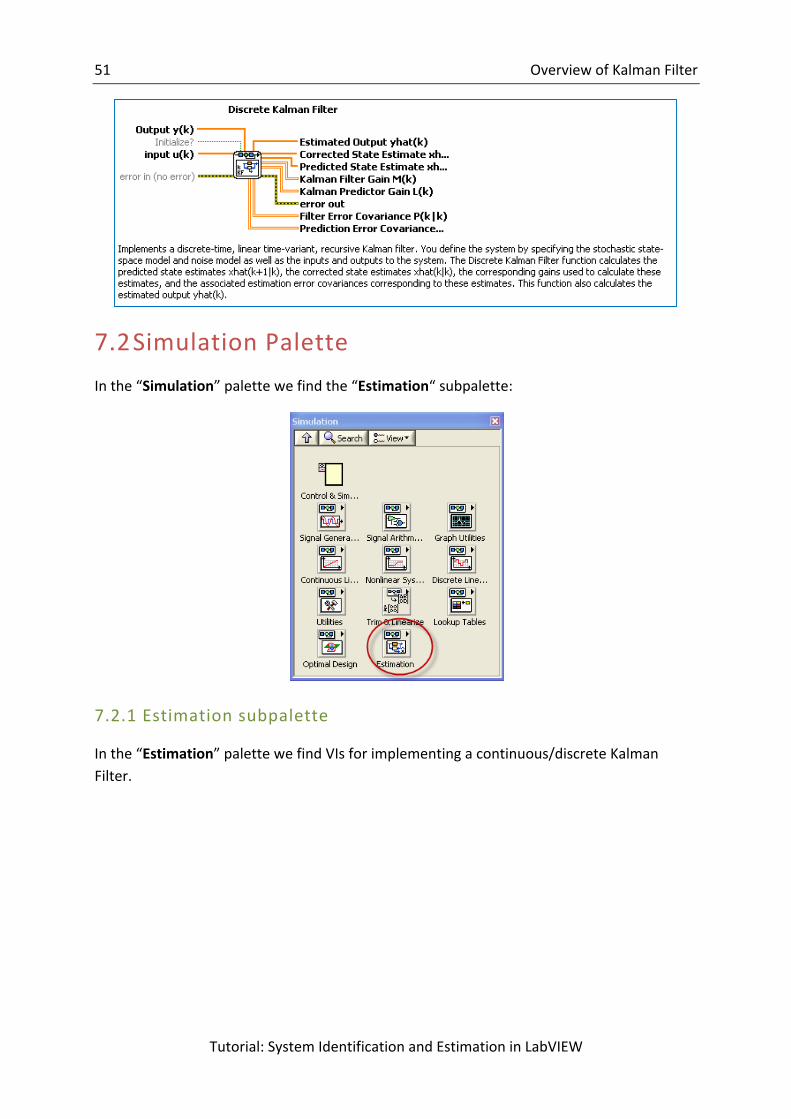
BelowweseetheDiscreteKalmanFilterimplementationinLabVIEW:
TheKalmanFilterfornonlinearmodelsiscalledthe“ExtendedKalmanFilter”.
27 StateEstimationwithKalmanFilter
Tutorial:SystemIdentificationandEstimationinLabVIEW
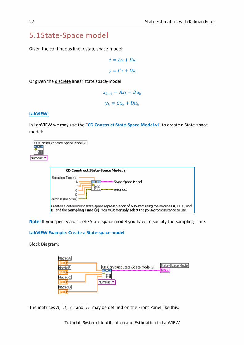
5.1 State-SpacemodelGiventhecontinuouslinearstatespace-model:
𝑥 = 𝐴𝑥 + 𝐵𝑢
𝑦 = 𝐶𝑥 + 𝐷𝑢
Orgiventhediscretelinearstatespace-model
𝑥JK7 = 𝐴𝑥J + 𝐵𝑢J
𝑦J = 𝐶𝑥J + 𝐷𝑢J
LabVIEW:
InLabVIEWwemayusethe“CDConstructState-SpaceModel.vi”tocreateaState-spacemodel:
Note!IfyouspecifyadiscreteState-spacemodelyouhavetospecifytheSamplingTime.
LabVIEWExample:CreateaState-spacemodel
BlockDiagram:
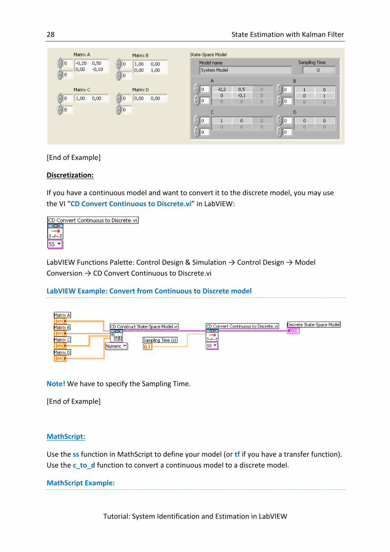
Thematrices𝐴, 𝐵, 𝐶 and 𝐷 maybedefinedontheFrontPanellikethis:
28 StateEstimationwithKalmanFilter
Tutorial:SystemIdentificationandEstimationinLabVIEW
[EndofExample]
Discretization:
Ifyouhaveacontinuousmodelandwanttoconvertittothediscretemodel,youmayusetheVI“CDConvertContinuoustoDiscrete.vi”inLabVIEW:
LabVIEWFunctionsPalette:ControlDesign&Simulation→ControlDesign→ModelConversion→CDConvertContinuoustoDiscrete.vi
LabVIEWExample:ConvertfromContinuoustoDiscretemodel
Note!WehavetospecifytheSamplingTime.
[EndofExample]
MathScript:
UsethessfunctioninMathScripttodefineyourmodel(ortfifyouhaveatransferfunction).Usethec_to_dfunctiontoconvertacontinuousmodeltoadiscretemodel.
MathScriptExample:
29 StateEstimationwithKalmanFilter
Tutorial:SystemIdentificationandEstimationinLabVIEW
GiventhefollowingState-spacemodel:
𝑥7𝑥8
=0 1
−𝑘𝑚
−𝑐𝑚
N
𝑥7𝑥8 +
01𝑚O
𝑢
𝑦 = 1 0P
𝑥7𝑥8
ThefollowingMathScriptCodecreatesthismodel:
c=1; m=1; k=1; A = [0 1; -k/m -c/m]; B = [0; 1/m]; C = [1 0]; ssmodel = ss(A, B, C)
Ifyouwanttofindthediscretemodelusethec_to_dfunction:
Ts=0.1 % Sampling Time discretemodel = c_to_d(ssmodel, Ts)
[EndofExample]
5.2 ObservabilityAnecessaryconditionfortheKalmanFiltertoworkcorrectlyisthatthesystemforwhichthestatesaretobeestimated,isobservable.Therefore,youshouldcheckforObservabilitybeforeapplyingtheKalmanFilter.
TheObservabilitymatrixisdefinedas:
𝑂 =𝐶𝐶𝐴⋮
𝐶𝐴I>7
Wherenisthesystemorder(numberofstatesintheState-spacemodel).
→Asystemofordernisobservableif 𝑶 isfullrank,meaningtherankof 𝑶 isequalton.
LabVIEW:
TheLabVIEWControlDesignandSimulationModulehaveaVI(ObservabilityMatrix.vi)forfindingtheObservabilitymatrixandcheckifastates-pacemodelisObservable.

30 StateEstimationwithKalmanFilter
Tutorial:SystemIdentificationandEstimationinLabVIEW
LabVIEWFunctionsPalette:ControlDesign&Simulation→ControlDesign→State-SpaceModelAnalysis→CDObservabilityMatrix.vi
Note!InLabVIEW 𝑁 isusedasasymbolfortheObservabilitymatrix.
LabVIEWExample:CheckforObservability
[EndofExample]
MathScript:
InMathScriptyoumayusetheobsvmxfunctiontofindtheObservabilitymatrix.YoumaythenusetherankfunctioninordertofindtherankoftheObservabilitymatrix.
MathScriptExample:
ThefollowingMathScriptCodecheckforObservability:
% Check for Observability: O = obsvmx (discretemodel) r = rank(O)
[EndofExample]
5.3 IntroductiontotheStateEstimatorContinuousModel:

31 StateEstimationwithKalmanFilter
Tutorial:SystemIdentificationandEstimationinLabVIEW
Giventhecontinuouslinearstatespacemodel:
𝑥 = 𝐴𝑥 + 𝐵𝑢 + 𝐺𝑤
𝑦 = 𝐶𝑥 + 𝐷𝑢 + 𝐻𝑣
oringeneral:
𝑥 = 𝑓(𝑥, 𝑢) + 𝐺𝑤
𝑦 = 𝑔(𝑥, 𝑢) + 𝐻𝑣
DiscreteModel:
Giventhediscretelinearstatespacemodel:
𝑥JK7 = 𝐴𝑥J + 𝐵𝑢J + 𝐺𝑤J
𝑦J = 𝐶𝑥J + 𝐷𝑢J + 𝐻𝑣J
oringeneral:
𝑥JK7 = 𝑓(𝑥J, 𝑢J) + 𝐺𝑤J
𝑦J = 𝑔(𝑥J, 𝑢J) + 𝐻𝑣J
Where 𝑣 isuncorrelatedwhiteprocessnoisewithzeromeanandcovariancematrix 𝑄 andwisuncorrelatedwhitemeasurementsnoisewithzeromeanandcovariancematrix,i.e.suchthat
𝑄 = 𝐸{𝑤𝑤`}
𝑅 = 𝐸{𝑣𝑣`}
𝐸{𝑤} istheexpectedvalueormeanoftheprocessnoisevector.
𝐸{𝑣}istheexpectedvalueormeanofthemeasurementnoisevector.
Itisnormaltolet 𝑄 and 𝑅 bediagonalmatrices:
𝑄 =
𝑞77 0 0 00 𝑞88 0 00 0 ⋱ 00 0 0 𝑞II
, 𝑅 =
𝑟77 0 0 00 𝑟88 0 00 0 ⋱ 00 0 0 𝑟ee
𝐺 istheprocessnoisegainmatrix,andyounormallyset 𝐺 equaltotheIdentitymatrix 𝐼:

32 StateEstimationwithKalmanFilter
Tutorial:SystemIdentificationandEstimationinLabVIEW
𝐺 =
1 0 0 00 1 0 00 0 ⋱ 00 0 0 1
𝐻 isthemeasurementnoisegainmatrix,andyounormallyset 𝐻 = 0
StateEstimator:
Thestateestimatorisgivenby:
𝑥JK7 = 𝐴𝑥J + 𝐵𝑢J + 𝐾(𝑦 − 𝑦)
𝑦J = 𝐶𝑥J
Where 𝐾 istheKalmanFilterGain
Itcanbefoundthat:
𝐾 = 𝑋𝐶`𝑄>7
Where 𝑋 isthesolutiontotheRiccatiequation.ItiscommontousethesteadystatesolutionoftheRiccatiequation(AlgebraicRiccatiEquation),i.e., 𝑋 = 0.
Note! 𝑄 and 𝑅 isusedastuning/weightingmatriceswhendesigningtheKalmanFilterGain 𝐾.
BelowweseeaBlockDiagramofa(discrete)KalmanFilter/StateEstimator:

33 StateEstimationwithKalmanFilter
Tutorial:SystemIdentificationandEstimationinLabVIEW
LabVIEW:
InLabVIEWDesignandSimulationModuleweusethe“CDKalmanGain.vi”inordertofindK:
LabVIEWFunctionsPalette:ControlDesign&Simulation→ControlDesign→StateFeedbackDesign→CDKalmanGain.vi
Note!InLabVIEW 𝐿 isusedasasymbolfortheKalmanFilterGainmatrix.
Note!The“KalmanFilterGain.vi”ispolymorphic,dependingonwhatkindofmodel(deterministic/stochasticorcontinuous/discrete)youwiretothisVI,theinputschangesautomaticallyoryoumayusethepolymorphicselectorbelowtheVI:
DeterministicandContinuous:
StochasticandContinuous:
DeterministicandDiscrete:
StochasticandDiscrete:

34 StateEstimationwithKalmanFilter
Tutorial:SystemIdentificationandEstimationinLabVIEW
LabVIEWExample:FindtheKalmanGain
BlockDiagram:
FrontPanel:
[EndofExample]
MathScript:
Usethefunctionskalman,kalman_dorlqetofindtheKalmangainmatrix.
Function Description Example
kalman Calculatestheoptimalsteady-stateKalmangainKthatminimizesthecovarianceofthestateestimationerror.YoucanusethisfunctiontocalculateKforcontinuousanddiscretesystemmodels.
>>[SysKal, K]=kalman(ssmodel, Q, R)
35 StateEstimationwithKalmanFilter
Tutorial:SystemIdentificationandEstimationinLabVIEW
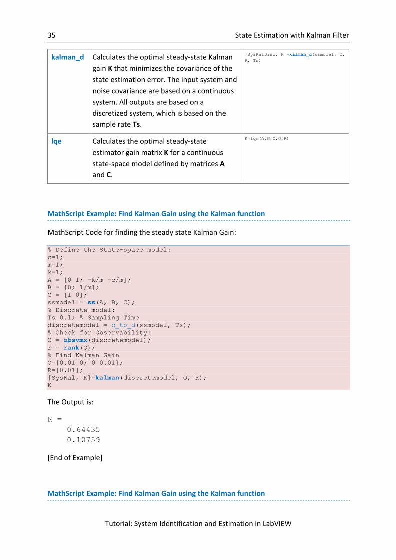
kalman_d Calculatestheoptimalsteady-stateKalmangainKthatminimizesthecovarianceofthestateestimationerror.Theinputsystemandnoisecovariancearebasedonacontinuoussystem.Alloutputsarebasedonadiscretizedsystem,whichisbasedonthesamplerateTs.
[SysKalDisc, K]=kalman_d(ssmodel, Q, R, Ts)
lqe Calculatestheoptimalsteady-stateestimatorgainmatrixKforacontinuousstate-spacemodeldefinedbymatricesAandC.
K=lqe(A,G,C,Q,R)
MathScriptExample:FindKalmanGainusingtheKalmanfunction
MathScriptCodeforfindingthesteadystateKalmanGain:
% Define the State-space model: c=1; m=1; k=1; A = [0 1; -k/m -c/m]; B = [0; 1/m]; C = [1 0]; ssmodel = ss(A, B, C); % Discrete model: Ts=0.1; % Sampling Time discretemodel = c_to_d(ssmodel, Ts); % Check for Observability: O = obsvmx(discretemodel); r = rank(O); % Find Kalman Gain Q=[0.01 0; 0 0.01]; R=[0.01]; [SysKal, K]=kalman(discretemodel, Q, R); K
TheOutputis:
K = 0.64435 0.10759
[EndofExample]
MathScriptExample:FindKalmanGainusingtheKalmanfunction
36 StateEstimationwithKalmanFilter
Tutorial:SystemIdentificationandEstimationinLabVIEW
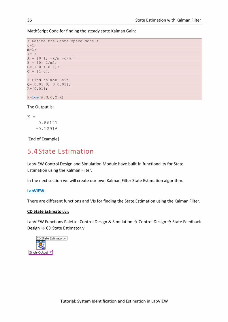
MathScriptCodeforfindingthesteadystateKalmanGain:
% Define the State-space model: c=1; m=1; k=1; A = [0 1; -k/m -c/m]; B = [0; 1/m]; G=[1 0 ; 0 1]; C = [1 0]; % Find Kalman Gain Q=[0.01 0; 0 0.01]; R=[0.01]; K=lqe(A,G,C,Q,R)
TheOutputis:
K = 0.86121 -0.12916
[EndofExample]
5.4 StateEstimationLabVIEWControlDesignandSimulationModulehavebuilt-infunctionalityforStateEstimationusingtheKalmanFilter.
InthenextsectionwewillcreateourownKalmanFilterStateEstimationalgorithm.
LabVIEW:
TherearedifferentfunctionsandVIsforfindingtheStateEstimationusingtheKalmanFilter.
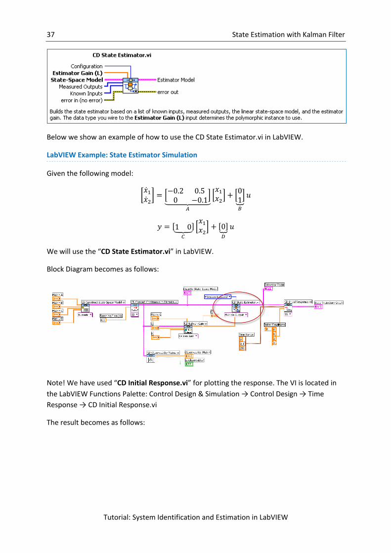
CDStateEstimator.vi:
LabVIEWFunctionsPalette:ControlDesign&Simulation→ControlDesign→StateFeedbackDesign→CDStateEstimator.vi
37 StateEstimationwithKalmanFilter
Tutorial:SystemIdentificationandEstimationinLabVIEW
BelowweshowanexampleofhowtousetheCDStateEstimator.viinLabVIEW.
LabVIEWExample:StateEstimatorSimulation
Giventhefollowingmodel:
𝑥7𝑥8
= −0.2 0.50 −0.1
N
𝑥7𝑥8 + 0
1O
𝑢
𝑦 = 1 0P
𝑥7𝑥8 + 0
k𝑢
Wewillusethe“CDStateEstimator.vi”inLabVIEW.
BlockDiagrambecomesasfollows:
Note!Wehaveused“CDInitialResponse.vi”forplottingtheresponse.TheVIislocatedintheLabVIEWFunctionsPalette:ControlDesign&Simulation→ControlDesign→TimeResponse→CDInitialResponse.vi
Theresultbecomesasfollows:
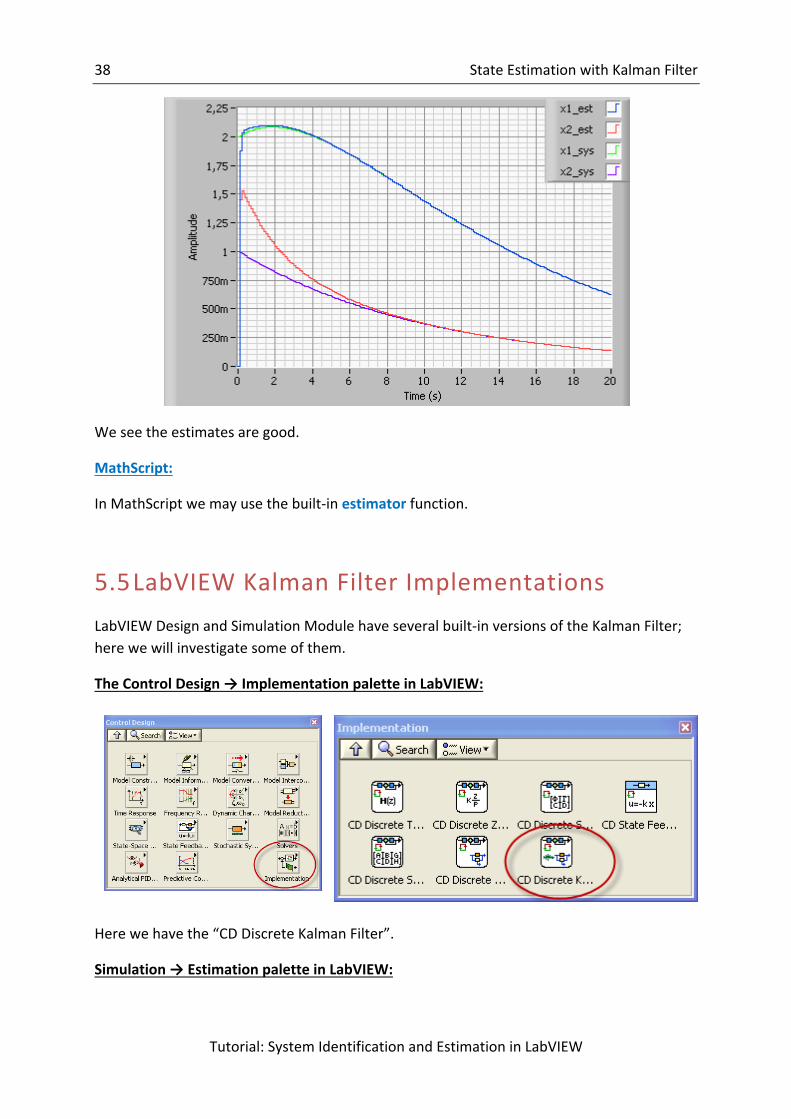
38 StateEstimationwithKalmanFilter
Tutorial:SystemIdentificationandEstimationinLabVIEW
Weseetheestimatesaregood.
MathScript:
InMathScriptwemayusethebuilt-inestimatorfunction.
5.5 LabVIEWKalmanFilterImplementationsLabVIEWDesignandSimulationModulehaveseveralbuilt-inversionsoftheKalmanFilter;herewewillinvestigatesomeofthem.
TheControlDesign→ImplementationpaletteinLabVIEW:
Herewehavethe“CDDiscreteKalmanFilter”.
Simulation→EstimationpaletteinLabVIEW:

39 StateEstimationwithKalmanFilter
Tutorial:SystemIdentificationandEstimationinLabVIEW
Herewehaveimplementationsfor:
• ContinuousKalmanFilter• ContinuousExtendedKalmanFilter• DiscreteKalmanFilter• DiscreteExtendedKalmanFilter
Wewillgothroughthe“DiscreteKalmanFilter”indetailandshowsomeexamples.
DiscreteKalmanFilter:
LabVIEWFunctionsPalette:ControlDesign&Simulation→Simulation→Estimation→DiscreteKalmanFilter
Bydefaultyouneedtowiretheinput(𝑢)andoutput(𝑦)vectors:
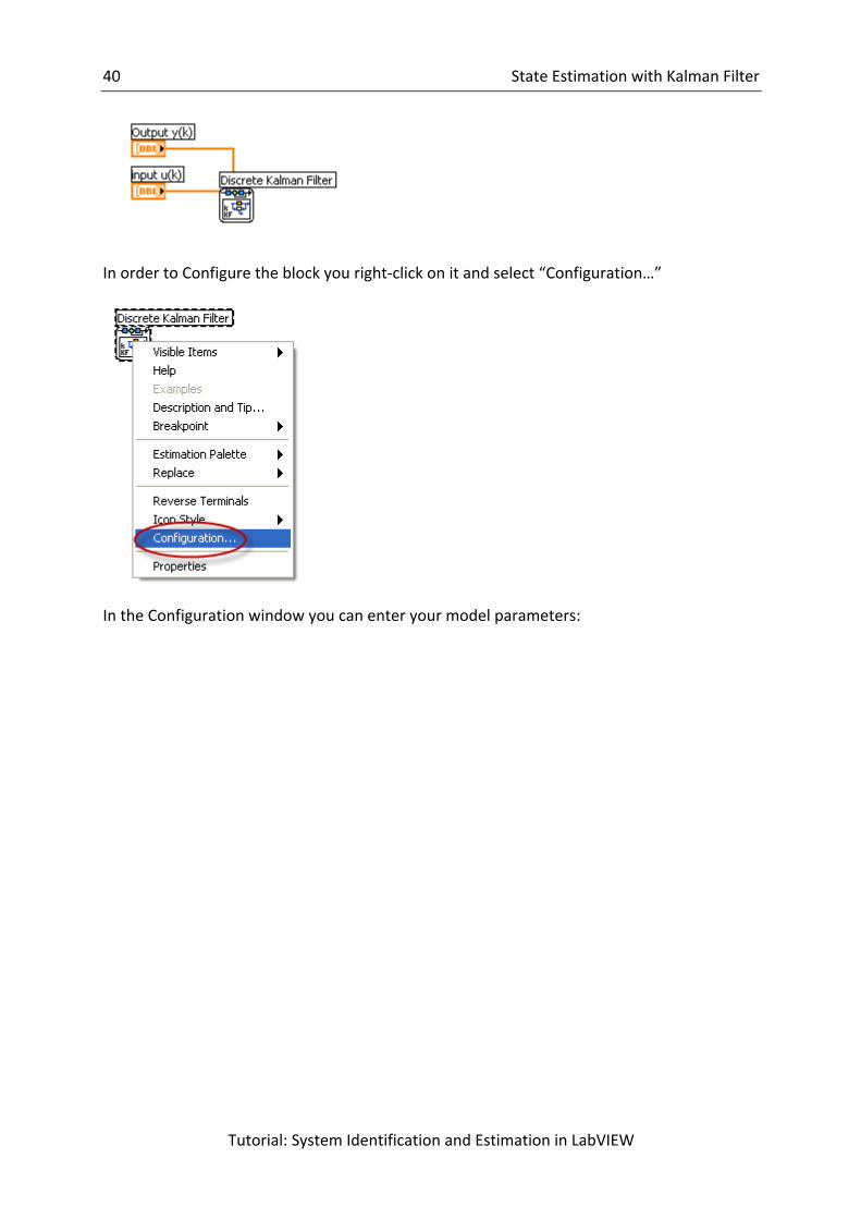
40 StateEstimationwithKalmanFilter
Tutorial:SystemIdentificationandEstimationinLabVIEW
InordertoConfiguretheblockyouright-clickonitandselect“Configuration…”
IntheConfigurationwindowyoucanenteryourmodelparameters:

41 StateEstimationwithKalmanFilter
Tutorial:SystemIdentificationandEstimationinLabVIEW
Ifyouselect“Terminal”inthe“Parametersource”youmaycreateyourmodelinLabVIEWcodelikethis:
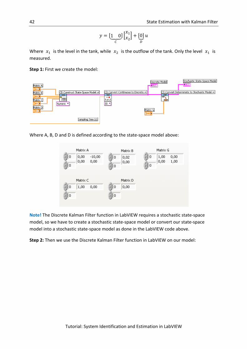
LabVIEWExample:DiscreteKalmanFilter
Giventhefollowinglinearstate-spacemodelofawatertank:
𝑥7𝑥8
= 0 −100 0
N
𝑥7𝑥8 + 0.02
0O
𝑢
42 StateEstimationwithKalmanFilter
Tutorial:SystemIdentificationandEstimationinLabVIEW
𝑦 = 1 0P
𝑥7𝑥8 + 0
k𝑢
Where 𝑥7 isthelevelinthetank,while 𝑥8 istheoutflowofthetank.Onlythelevel 𝑥7 ismeasured.
Step1:Firstwecreatethemodel:
WhereA,B,DandDisdefinedaccordingtothestate-spacemodelabove:
Note!TheDiscreteKalmanFilterfunctioninLabVIEWrequiresastochasticstate-spacemodel,sowehavetocreateastochasticstate-spacemodelorconvertourstate-spacemodelintoastochasticstate-spacemodelasdoneintheLabVIEWcodeabove.
Step2:ThenweusetheDiscreteKalmanFilterfunctioninLabVIEWonourmodel:

43 StateEstimationwithKalmanFilter
Tutorial:SystemIdentificationandEstimationinLabVIEW
TheDiscreteKalmanFilterfunctionalsorequiresaNoisemodel,sowecreateanoisemodelfromour 𝑄 and 𝑅 matricesasdoneintheLabVIEWcodeabove.
Theresultsareasfollows:
Weseetheresultisverygood.
[EndofExample]

44
6 CreateyourownKalmanFilterfromScratch
InthischapterwewillcreateourownKalmanFilterAlgorithmfromscratch.
6.1 TheKalmanFilterAlgorithmLabVIEWDesignandSimulationModulehaveseveralbuilt-inversionsoftheKalmanFilter,butinthischapterwewillcreateourownKalmanFilteralgorithm.
HereisastepbystepKalmanFilteralgorithmwhichcanbedirectlyimplementedinaprogramminglanguage,suchasLabVIEW.Youmay,e.g.,implementitinstandardLabVIEWcodeoraFormulaNodeinLabVIEW.
PreStep:FindthesteadystateKalmanGainK
Kistime-varying,butyounormallyimplementthesteadystateversionofKalmanGainK.Usethe“CDKalmanGain.vi”inLabVIEWoroneofthefunctionskalman,kalman_dorlqeinMathScript.
InitStep:SettheinitialApriori(Predicted)stateestimate
𝑥6 = 𝑥6
Step1:FindMeasurementmodelupdate
𝑦J = 𝑔(𝑥J, 𝑢J)
ForLinearState-spacemodel:
𝑦J = 𝐶𝑥J + 𝐷𝑢J
Step2:FindtheEstimatorError
𝑒J = 𝑦J − 𝑦J
Step3:FindtheAposteriori(Corrected)stateestimate
𝑥J = 𝑥J + 𝐾𝑒J
WhereKistheKalmanFilterGain.UsethesteadystateKalmanGainorcalculatethetime-varyingKalmanGain.
Step4:FindtheApriori(Predicted)stateestimateupdate
𝑥JK7 = 𝑓(𝑥J, 𝑢J)

45 CreateyourownKalmanFilterfromScratch
Tutorial:SystemIdentificationandEstimationinLabVIEW
ForLinearState-spacemodel:
𝑥JK7 = 𝐴𝑥J + 𝐵𝑢J
Step1-4goesinsidealoopinyourprogram.
Thisisthealgorithmwewillimplementintheexamplebelow.
6.2 ExamplesLabVIEWExample:KalmanFilteralgorithm
Giventhefollowinglinearstate-spacemodelofawatertank:
𝑥7𝑥8
= 0 −100 0
N
𝑥7𝑥8 + 0.02
0O
𝑢
𝑦 = 1 0P
𝑥7𝑥8 + 0
k𝑢
Where 𝑥7 isthelevelinthetank,while 𝑥8 istheoutflowofthetank.Onlythelevel 𝑥7 ismeasured.
FirstwehavetofindthesteadystateKalmanFilterGainandcheckforObservability:
Thenweruntherealprocess(orsimulatedmodel)inparallelwiththeKalmanFilterinordertofindestimatesfor 𝑥7 and 𝑥8:
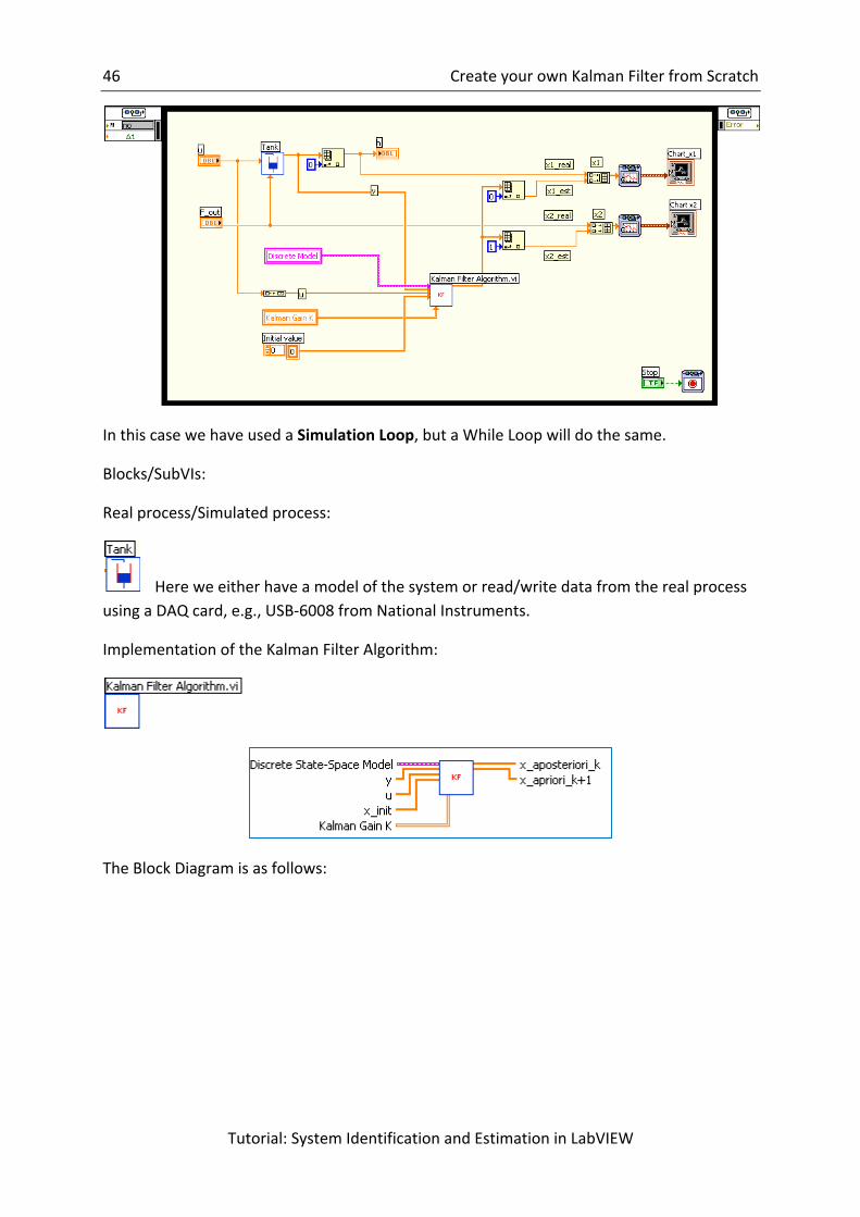
46 CreateyourownKalmanFilterfromScratch
Tutorial:SystemIdentificationandEstimationinLabVIEW
InthiscasewehaveusedaSimulationLoop,butaWhileLoopwilldothesame.
Blocks/SubVIs:
Realprocess/Simulatedprocess:
Hereweeitherhaveamodelofthesystemorread/writedatafromtherealprocessusingaDAQcard,e.g.,USB-6008fromNationalInstruments.
ImplementationoftheKalmanFilterAlgorithm:
TheBlockDiagramisasfollows:

47 CreateyourownKalmanFilterfromScratch
Tutorial:SystemIdentificationandEstimationinLabVIEW
Thisisageneralimplementationandwillworkforalllineardiscretesystems.
Theresultsareasfollows:

48 CreateyourownKalmanFilterfromScratch
Tutorial:SystemIdentificationandEstimationinLabVIEW
[EndofExample]

49
7 OverviewofKalmanFilterVIsInLabVIEWthereareseveralVIsandfunctionsusedforKalmanFilterimplementations.
7.1 ControlDesignPaletteInthe“ControlDesign”palettewefindsubpalettesfor“StateFeedbackDesign”and“Implementation”:
7.1.1 StateFeedbackDesignsubpalette
Inthe“StateFeedbackDesign”subpalettewefindVIsforcalculationtheKalmanGain,etc.
→UsetheStateFeedbackDesignVIstocalculatecontrollerandobservergainsforclosed-loopstatefeedbackcontrolortoestimateastate-spacemodel.YoualsocanuseState
50 OverviewofKalmanFilter
Tutorial:SystemIdentificationandEstimationinLabVIEW
FeedbackDesignVIstoconfigureandteststate-spacecontrollersandstateestimatorsintimedomains.
KalmanFilterGainVI:
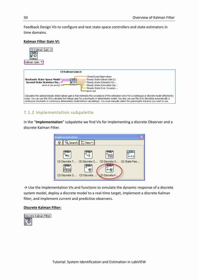
7.1.2 Implementationsubpalette
Inthe“Implementation”subpalettewefindVIsforimplementingadiscreteObserverandadiscreteKalmanFilter.
→UsetheImplementationVIsandfunctionstosimulatethedynamicresponseofadiscretesystemmodel,deployadiscretemodeltoareal-timetarget,implementadiscreteKalmanfilter,andimplementcurrentandpredictiveobservers.
DiscreteKalmanFilter:
51 OverviewofKalmanFilter
Tutorial:SystemIdentificationandEstimationinLabVIEW
7.2 SimulationPaletteInthe“Simulation”palettewefindthe“Estimation“subpalette:
7.2.1 Estimationsubpalette
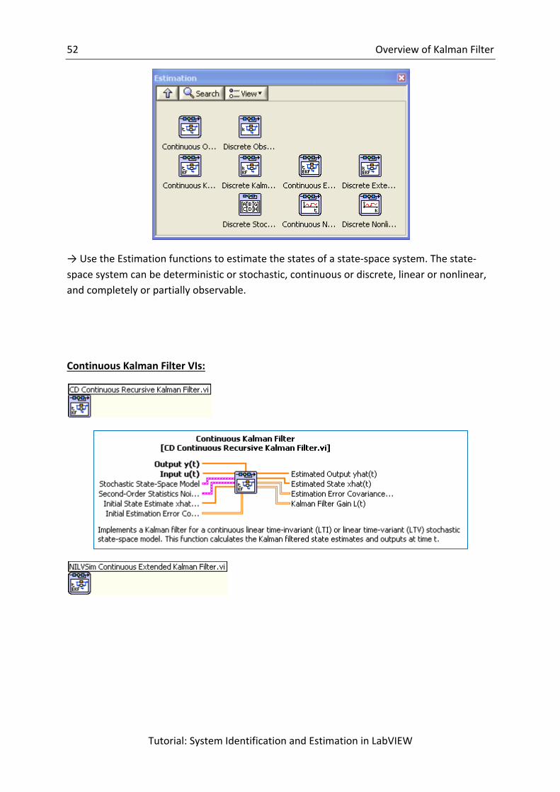
Inthe“Estimation”palettewefindVIsforimplementingacontinuous/discreteKalmanFilter.
52 OverviewofKalmanFilter
Tutorial:SystemIdentificationandEstimationinLabVIEW
→UsetheEstimationfunctionstoestimatethestatesofastate-spacesystem.Thestate-spacesystemcanbedeterministicorstochastic,continuousordiscrete,linearornonlinear,andcompletelyorpartiallyobservable.
ContinuousKalmanFilterVIs:

53 OverviewofKalmanFilter
Tutorial:SystemIdentificationandEstimationinLabVIEW
DiscreteKalmanFilterVIs:
54
8 StateEstimationwithObserversinLabVIEW
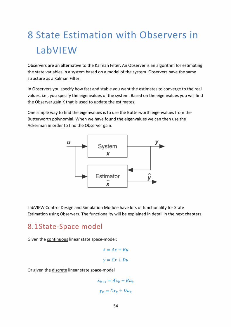
ObserversareanalternativetotheKalmanFilter.AnObserverisanalgorithmforestimatingthestatevariablesinasystembasedonamodelofthesystem.ObservershavethesamestructureasaKalmanFilter.
InObserversyouspecifyhowfastandstableyouwanttheestimatestoconvergetotherealvalues,i.e.,youspecifytheeigenvaluesofthesystem.BasedontheeigenvaluesyouwillfindtheObservergainKthatisusedtoupdatetheestimates.
OnesimplewaytofindtheeigenvaluesistousetheButterwortheigenvaluesfromtheButterworthpolynomial.WhenwehavefoundtheeigenvalueswecanthenusetheAckermaninordertofindtheObservergain.
LabVIEWControlDesignandSimulationModulehavelotsoffunctionalityforStateEstimationusingObservers.Thefunctionalitywillbeexplainedindetailinthenextchapters.
8.1 State-SpacemodelGiventhecontinuouslinearstatespace-model:
𝑥 = 𝐴𝑥 + 𝐵𝑢
𝑦 = 𝐶𝑥 + 𝐷𝑢
Orgiventhediscretelinearstatespace-model
𝑥JK7 = 𝐴𝑥J + 𝐵𝑢J
𝑦J = 𝐶𝑥J + 𝐷𝑢J
55 StateEstimationwithObserversinLabVIEW
Tutorial:SystemIdentificationandEstimationinLabVIEW
LabVIEW:
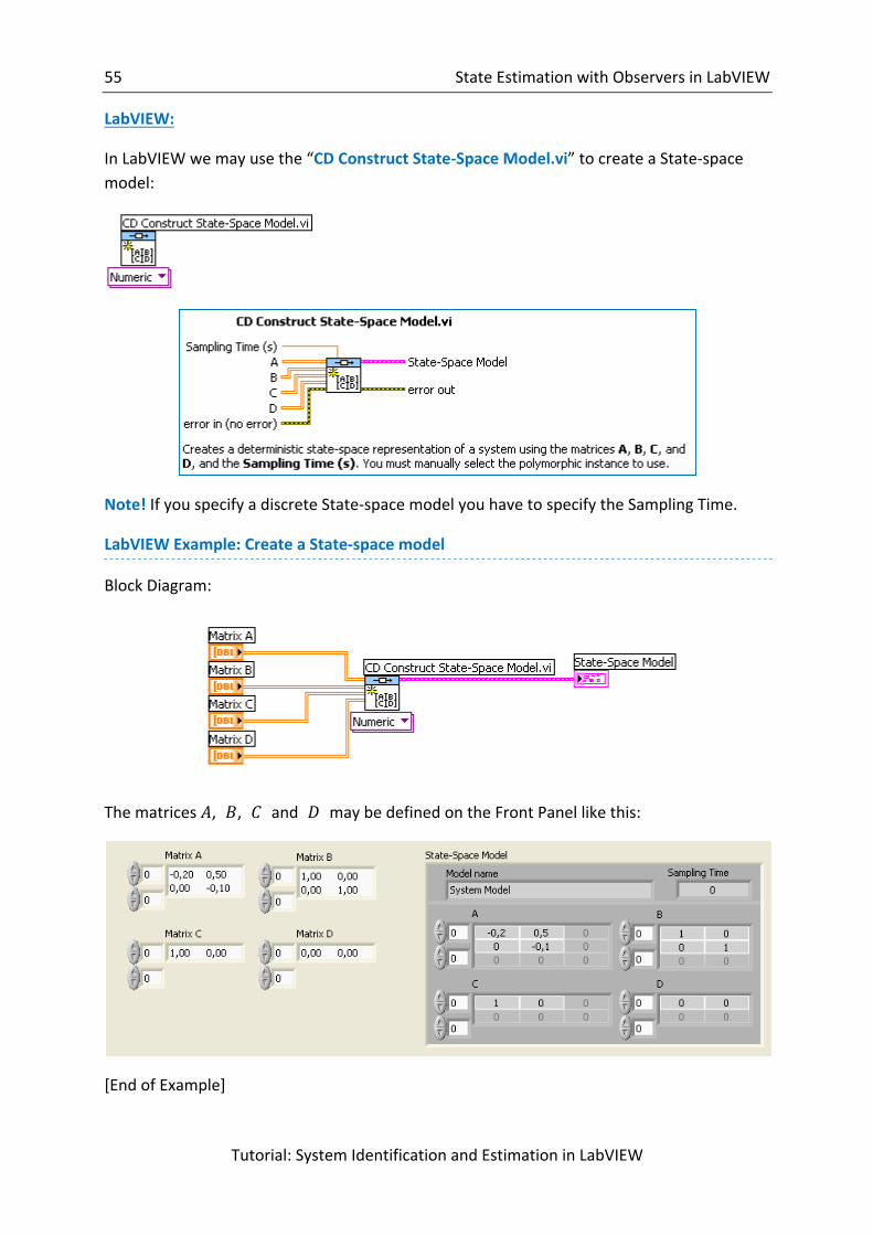
InLabVIEWwemayusethe“CDConstructState-SpaceModel.vi”tocreateaState-spacemodel:
Note!IfyouspecifyadiscreteState-spacemodelyouhavetospecifytheSamplingTime.
LabVIEWExample:CreateaState-spacemodel
BlockDiagram:
Thematrices𝐴, 𝐵, 𝐶 and 𝐷 maybedefinedontheFrontPanellikethis:
[EndofExample]
56 StateEstimationwithObserversinLabVIEW
Tutorial:SystemIdentificationandEstimationinLabVIEW
8.2 EigenvaluesOnesimplewaytofindtheeigenvaluesistousetheButterwortheigenvaluesfromtheButterworthpolynomial.
ButterwortPolynomial:
TheButterworthPolynomialisdefinedas:
𝐵I 𝑠 = 𝑎I𝑠I +…+ 𝑎8𝑠8 + 𝑎7𝑠 + 1
where 𝑎6 = 1, 𝑎7, 𝑎8, … , 𝑎I arethecoefficientsintheButterworthPolynomial.
Herewewillusea2.orderButterworthPolynomial,whichisdefinedas:
𝐵8 𝑠 = 𝑎8𝑠8 + 𝑎7𝑠 + 1
where 𝑎6 = 1, 𝑎7 = 2𝑇, 𝑎8 = 𝑇8.
Thisgives:
𝐵8 𝑠 = 𝑇8𝑠8 + 2𝑇𝑠 + 1
wheretheparameter 𝑇 isusedtodefinedthespeedoftheresponseaccordingto:
𝑇e ≈ 𝑛𝑇
where 𝑇e isdefinedastheObserverresponsetimewherethestepresponsereach63%ofthesteadystatevalueoftheresponse.
→Sowewilluse 𝑇e asthetuningparameterfortheObserver.
LabVIEW:
InLabVIEWwecanusethe“PolynomialRoots.vi”tofindtherootsbasedontheButterworthPolynomial
LabVIEWFunctionsPalette:Mathematics→Polynomial→PolynomialRoots.vi
57 StateEstimationwithObserversinLabVIEW
Tutorial:SystemIdentificationandEstimationinLabVIEW
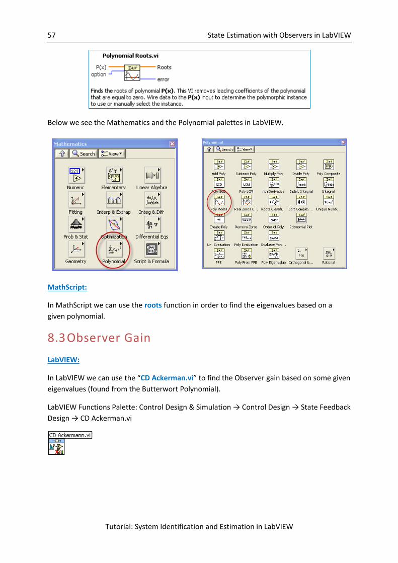
BelowweseetheMathematicsandthePolynomialpalettesinLabVIEW.
MathScript:
InMathScriptwecanusetherootsfunctioninordertofindtheeigenvaluesbasedonagivenpolynomial.
8.3 ObserverGainLabVIEW:
InLabVIEWwecanusethe“CDAckerman.vi”tofindtheObservergainbasedonsomegiveneigenvalues(foundfromtheButterwortPolynomial).
LabVIEWFunctionsPalette:ControlDesign&Simulation→ControlDesign→StateFeedbackDesign→CDAckerman.vi

58 StateEstimationwithObserversinLabVIEW
Tutorial:SystemIdentificationandEstimationinLabVIEW
MathScript:
InMathScriptwecanusetheackerfunctioninordertofindtheObservergainbasedonsomegiveneigenvalues(foundfromtheButterwortPolynomial).
8.4 ObservabilityAnecessaryconditionfortheObservertoworkcorrectlyisthatthesystemforwhichthestatesaretobeestimated,isobservable.Therefore,youshouldcheckforObservabilitybeforeapplyingtheObserver.
TheObservabilitymatrixisdefinedas:
𝑂 =𝐶𝐶𝐴⋮
𝐶𝐴I>7
Wherenisthesystemorder(numberofstatesintheState-spacemodel).
→Asystemofordernisobservableif 𝑶 isfullrank,meaningtherankof 𝑶 isequalton.
LabVIEW:
TheLabVIEWControlDesignandSimulationModulehaveaVI(ObservabilityMatrix.vi)forfindingtheObservabilitymatrixandcheckifastates-pacemodelisObservable.
LabVIEWFunctionsPalette:ControlDesign&Simulation→ControlDesign→State-SpaceModelAnalysis→CDObservabilityMatrix.vi
59 StateEstimationwithObserversinLabVIEW
Tutorial:SystemIdentificationandEstimationinLabVIEW
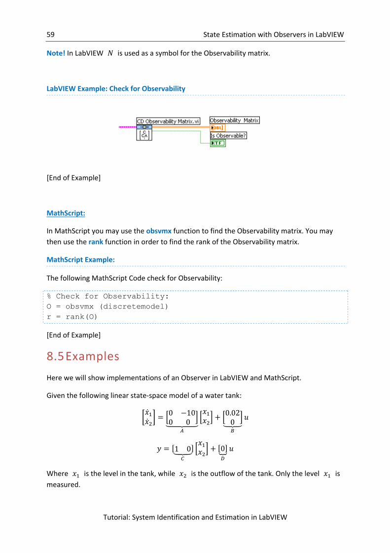
Note!InLabVIEW 𝑁 isusedasasymbolfortheObservabilitymatrix.
LabVIEWExample:CheckforObservability
[EndofExample]
MathScript:
InMathScriptyoumayusetheobsvmxfunctiontofindtheObservabilitymatrix.YoumaythenusetherankfunctioninordertofindtherankoftheObservabilitymatrix.
MathScriptExample:
ThefollowingMathScriptCodecheckforObservability:
% Check for Observability: O = obsvmx (discretemodel) r = rank(O)
[EndofExample]
8.5 ExamplesHerewewillshowimplementationsofanObserverinLabVIEWandMathScript.
Giventhefollowinglinearstate-spacemodelofawatertank:
𝑥7𝑥8
= 0 −100 0
N
𝑥7𝑥8 + 0.02
0O
𝑢
𝑦 = 1 0P
𝑥7𝑥8 + 0
k𝑢
Where 𝑥7 isthelevelinthetank,while 𝑥8 istheoutflowofthetank.Onlythelevel 𝑥7 ismeasured.
60 StateEstimationwithObserversinLabVIEW
Tutorial:SystemIdentificationandEstimationinLabVIEW
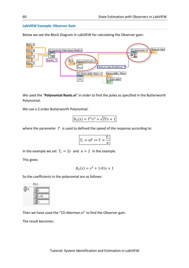
LabVIEWExample:ObserverGain
BelowweseetheBlockDiagraminLabVIEWforcalculatingtheObservergain:
Weusedthe“PolynomialRoots.vi”inordertofindthepolesasspecifiedintheButterworthPolynomial.
Weusea2.orderButterworthPolynomial:
𝐵8 𝑠 = 𝑇8𝑠8 + 2𝑇𝑠 + 1
wheretheparameter 𝑇 isusedtodefinedthespeedoftheresponseaccordingto:
𝑇e ≈ 𝑛𝑇 ↔ 𝑇 =𝑇e𝑛
Intheexampleweset 𝑇e = 2𝑠 and 𝑛 = 2 intheexample.
Thisgives:
𝐵8 𝑠 = 𝑠8 + 1.41𝑠 + 1
Sothecoefficientsinthepolynomialareasfollows:
Thenwehaveusedthe“CDAkerman.vi”tofindtheObservergain.
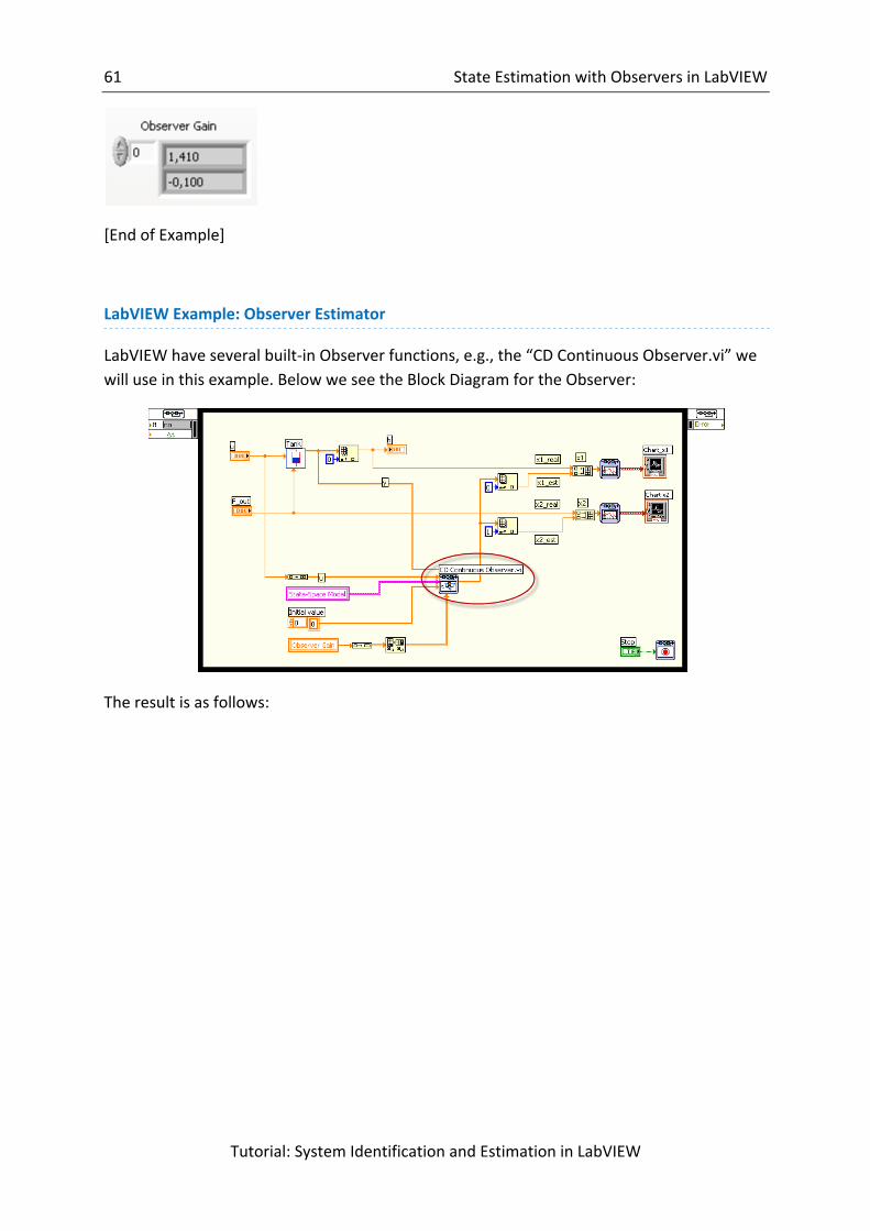
Theresultbecomes:
61 StateEstimationwithObserversinLabVIEW
Tutorial:SystemIdentificationandEstimationinLabVIEW
[EndofExample]
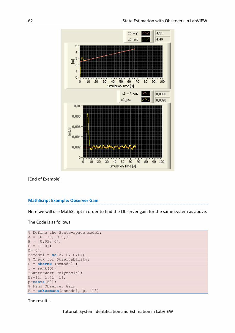
LabVIEWExample:ObserverEstimator
LabVIEWhaveseveralbuilt-inObserverfunctions,e.g.,the“CDContinuousObserver.vi”wewilluseinthisexample.BelowweseetheBlockDiagramfortheObserver:
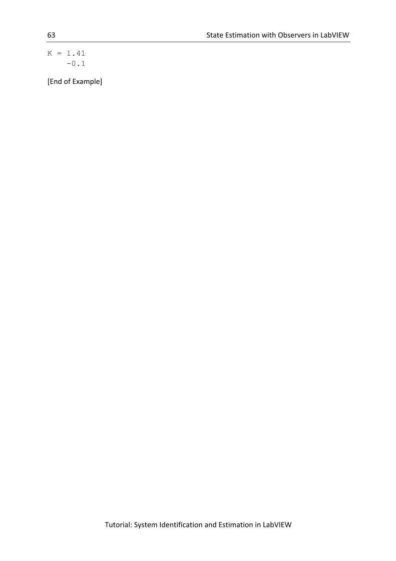
Theresultisasfollows:
62 StateEstimationwithObserversinLabVIEW
Tutorial:SystemIdentificationandEstimationinLabVIEW
[EndofExample]
MathScriptExample:ObserverGain
HerewewilluseMathScriptinordertofindtheObservergainforthesamesystemasabove.
TheCodeisasfollows:
% Define the State-space model: A = [0 -10; 0 0]; B = [0.02; 0]; C = [1 0]; D=[0]; ssmodel = ss(A, B, C,D); % Check for Observability: O = obsvmx (ssmodel); r = rank(O); %Butterwort Polynomial: B2=[1, 1.41, 1]; p=roots(B2); % Find Observer Gain K = ackermann(ssmodel, p, 'L')
Theresultis:
63 StateEstimationwithObserversinLabVIEW
Tutorial:SystemIdentificationandEstimationinLabVIEW
K = 1.41 -0.1
[EndofExample]
64
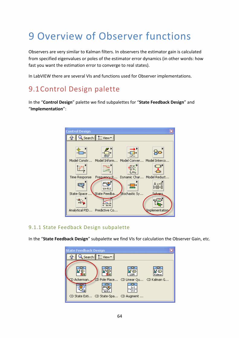
9 OverviewofObserverfunctionsObserversareverysimilartoKalmanfilters.Inobserverstheestimatorgainiscalculatedfromspecifiedeigenvaluesorpolesoftheestimatorerrordynamics(inotherwords:howfastyouwanttheestimationerrortoconvergetorealstates).
InLabVIEWthereareseveralVIsandfunctionsusedforObserverimplementations.
9.1 ControlDesignpaletteInthe“ControlDesign”palettewefindsubpalettesfor“StateFeedbackDesign”and“Implementation”:
9.1.1 StateFeedbackDesignsubpalette
Inthe“StateFeedbackDesign”subpalettewefindVIsforcalculationtheObserverGain,etc.
65 OverviewofObserverfunctions
Tutorial:SystemIdentificationandEstimationinLabVIEW
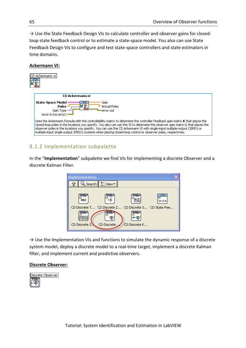
→UsetheStateFeedbackDesignVIstocalculatecontrollerandobservergainsforclosed-loopstatefeedbackcontrolortoestimateastate-spacemodel.YoualsocanuseStateFeedbackDesignVIstoconfigureandteststate-spacecontrollersandstateestimatorsintimedomains.
AckermannVI:
9.1.2 Implementationsubpalette
Inthe“Implementation”subpalettewefindVIsforimplementingadiscreteObserverandadiscreteKalmanFilter.
→UsetheImplementationVIsandfunctionstosimulatethedynamicresponseofadiscretesystemmodel,deployadiscretemodeltoareal-timetarget,implementadiscreteKalmanfilter,andimplementcurrentandpredictiveobservers.
DiscreteObserver:

66 OverviewofObserverfunctions
Tutorial:SystemIdentificationandEstimationinLabVIEW
9.2 SimulationpaletteInthe“Simulation”palettewefindthe“Estimation“sub-palette:
9.2.1 Estimationsubpalette
Inthe“Estimation”palettewefindVIsforimplementingcontinuous/discreteObserversandKalmanFilter.

67 OverviewofObserverfunctions
Tutorial:SystemIdentificationandEstimationinLabVIEW
→UsetheEstimationfunctionstoestimatethestatesofastate-spacesystem.Thestate-spacesystemcanbedeterministicorstochastic,continuousordiscrete,linearornonlinear,andcompletelyorpartiallyobservable.
ContinuousObserverVI:
DiscreteObserverVI:
68
PartIII:SystemIdentification

69
10 SystemIdentificationinLabVIEWThemodelcanbeinformofdifferentialequationsdevelopedfromphysicalprinciplesorfromtransferfunctionmodels,whichcanberegardedas“black-box”-modelswhichexpressestheinput-outputpropertyofthesystem.Someoftheparametersofthemodelcanhaveunknownoruncertainvalues,forexampleaheattransfercoefficientinathermalprocessorthetime-constantinatransferfunctionmodel.Wecantrytoestimatesuchparametersfrommeasurementstakenduringexperimentsonthesystem.
Herewewilldiscuss:
• ParameterEstimationandtheLeastSquareMethod(LS)• Sub-spacemethods/Black-Boxmethods• PolynomialModelEstimation:ARX/ARMAXmodelEstimation
InLabVIEWwecanusethe“SystemIdentificationPalette”.
The“SystemIdentification”paletteinLabVIEW:
InthenextchapterswewillusethedifferentfunctionalityavailableintheSystemIdentificationToolkit.

70 SystemIdentificationinLabVIEW
Tutorial:SystemIdentificationandEstimationinLabVIEW
10.1 ParameterEstimationwithLeastSquareMethod(LS)
ParameterEstimationusingtheLeastSquareMethod(LS)isusedtofindamodelwithunknownphysicalparametersinamathematicalmodel.
TheLeastsquaremethodcanbewrittenas:
𝑌 = Φ𝜃
Where
𝜽 istheunknownparametervector
𝑌 istheknownmeasurementvector
Φ istheknownregressionmatrix
Thesolutionfor 𝜃 maybefoundas:
𝜃 = Φ>7𝑌
Itcanbefoundthattheleastsquaresolutionfor 𝑌 = Φ𝑌 is:
𝜃st = (ΦuΦ)>7ΦuY
ImplementationinMathScript/MATLAB:
theta=inv(phi’*phi)* phi’*Y
orsimply:
theta=phi\Y
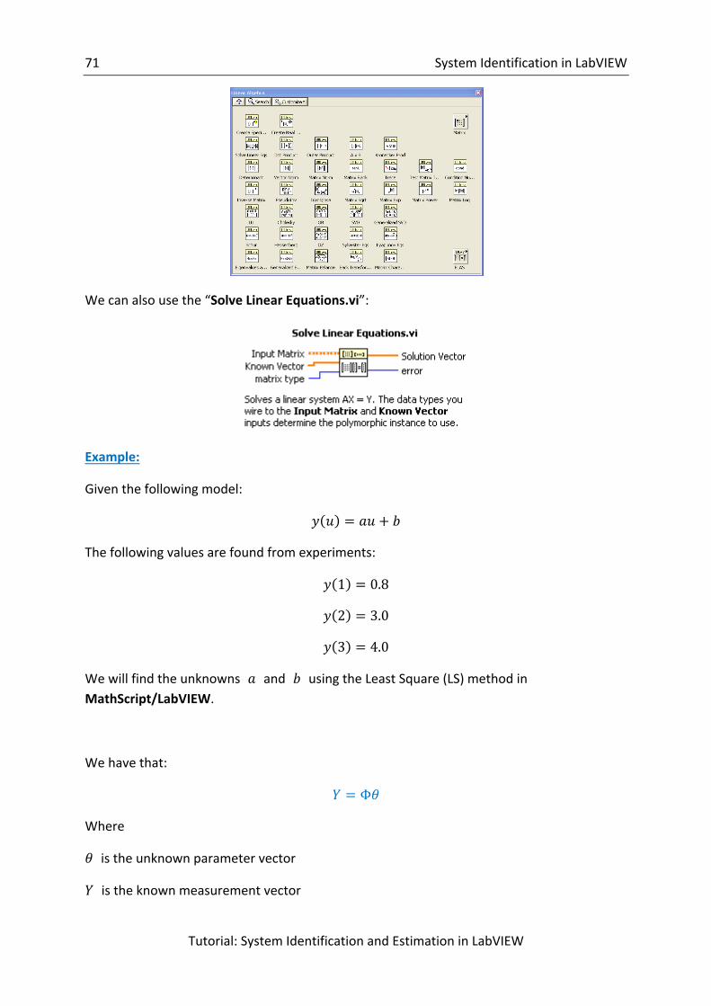
InLabVIEWwecanusetheblocks(“AxB.vi”,“TransposeMatrix.vi”,“InverseMatrix.vi”)inthe“LinearAlgebra”(locatedintheMathematicspalette)paletteinordertofintheLeastSquaresolution:
71 SystemIdentificationinLabVIEW
Tutorial:SystemIdentificationandEstimationinLabVIEW
Wecanalsousethe“SolveLinearEquations.vi”:
Example:
Giventhefollowingmodel:
𝑦 𝑢 = 𝑎𝑢 + 𝑏
Thefollowingvaluesarefoundfromexperiments:
𝑦 1 = 0.8
𝑦 2 = 3.0
𝑦 3 = 4.0
Wewillfindtheunknowns 𝑎 and 𝑏 usingtheLeastSquare(LS)methodinMathScript/LabVIEW.
Wehavethat:
𝑌 = Φ𝜃
Where
𝜃 istheunknownparametervector
𝑌 istheknownmeasurementvector

72 SystemIdentificationinLabVIEW
Tutorial:SystemIdentificationandEstimationinLabVIEW
Φ istheknownregressionmatrix
Thesolutionfor 𝜃 maybefoundas(if Φ isaquadraticmatrix):
𝜃 = Φ>7𝑌
Itcanbefoundthattheleastsquaresolutionfor 𝑌 = Φ𝜃 is:
𝜃st = (ΦuΦ)>7ΦuY
Weget:
0.8 = 𝑎 ∙ 1 + 𝑏
3.0 = 𝑎 ∙ 2 + 𝑏
4.0 = 𝑎 ∙ 3 + 𝑏
Thisbecomes:
0.83.04.0z
=1 12 13 1{
𝑎𝑏|
MathScript:
Wedefine 𝑌 and Φ inMathScriptandfind 𝜃 by:
phi = [1 1; 2 1; 3 1]; Y = [0.8 3.0 4.0]'; theta = inv(phi'*phi)* phi'*Y %or simply by theta=phi\Y
Theanswerbecomes:
theta = 1.6
-0.6
i.e.:
𝑎 = 1.6
𝑏 = −0.6
Thisgives:
73 SystemIdentificationinLabVIEW
Tutorial:SystemIdentificationandEstimationinLabVIEW
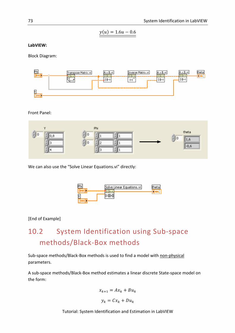
𝑦 𝑢 = 1.6𝑢 − 0.6
LabVIEW:
BlockDiagram:
FrontPanel:
Wecanalsousethe“SolveLinearEquations.vi”directly:
[EndofExample]
10.2 SystemIdentificationusingSub-spacemethods/Black-Boxmethods
Sub-spacemethods/Black-Boxmethodsisusedtofindamodelwithnon-physicalparameters.
Asub-spacemethods/Black-BoxmethodestimatesalineardiscreteState-spacemodelontheform:
𝑥JK7 = 𝐴𝑥J + 𝐵𝑢J
𝑦J = 𝐶𝑥J + 𝐷𝑢J

74 SystemIdentificationinLabVIEW
Tutorial:SystemIdentificationandEstimationinLabVIEW
LabVIEWoffersfunctionalityforthis.Inthe“ParametricModelEstimation”palettewefindthe“SIEstimateState-SpaceModel.vi”whichcanbeusedforsub-spaceidentification.
“ParametricModelEstimation”palette:
ThisVIestimatestheparametersofastate-spacemodelforanunknownsystem.
10.3 SystemIdentificationusingPolynomialModelEstimation:ARX/ARMAXmodelEstimation
LabVIEWoffersVIsforARX/ARMAXmodelestimationinthe“ParametricModelEstimation”palette.

75 SystemIdentificationinLabVIEW
Tutorial:SystemIdentificationandEstimationinLabVIEW
ForARXmodelswecanuse“SIEstimateARXmodel”:
ForARMAXmodelswecanuse“SIEstimateARMAXmodel”:
10.4 GeneratemodelDataInordertofindamodelweneedtogeneratedatabasedontherealprocess.Thestimulus(exitation)signalandtheresponsesignalwillthenbeinputtothefunctions/VIs(algorithms)inLabVIEWthatyouwillusetomodelyourprocess.
BelowweexplainhowwedothisinLabVIEW.
Datalogging:

76 SystemIdentificationinLabVIEW
Tutorial:SystemIdentificationandEstimationinLabVIEW
UseLabVIEWforexcitingtheprocessandloggingsignals.Useopen-loopexperiments(nofeedbackcontrolsystem).YoucanusetheWritetoMeasurementFilefunctionontheFileI/OpaletteinLabVIEWforwritingdatatotextfiles(usetheLVMdatafileformat,nottheTDMSfileformatwhichgivebinaryfiles).
IntheFileI/OpaletteinLabVIEWwehavelotsoffunctionalityforwritingandreadingfiles.
Belowweseethe“FileI/O”paletteinLabVIEW:
InthisTutorialwewillfocusonthe“WriteToMeasurementFile”and“ReadFromMeasurementFile”.
The“WriteToMeasurementFile”and“ReadFromMeasurementFile”isso-called“ExpressVIs”.WhenyoudragtheseVI’stotheBlockDiagram,aconfigurationdialogpops-upimmediately,likethis:

77 SystemIdentificationinLabVIEW
Tutorial:SystemIdentificationandEstimationinLabVIEW
Inthisconfigurationdialogyousetfilename,filetype,etc.
Notethatthese“ExpressVIs”havenoBlockDiagram.
10.4.1 Excitationsignals
Itisimportanttohaveagoodexcitationsignal,youcanusedifferentexcitationsignals,suchas:
• APRBSsignal(PseudoRandomBinarySignal) • AChirpSignal• AUp-downsignal
LabVIEW:
InLabVIEWyoucanusesomeofthefunctionsintheSignalGenerationpalette:
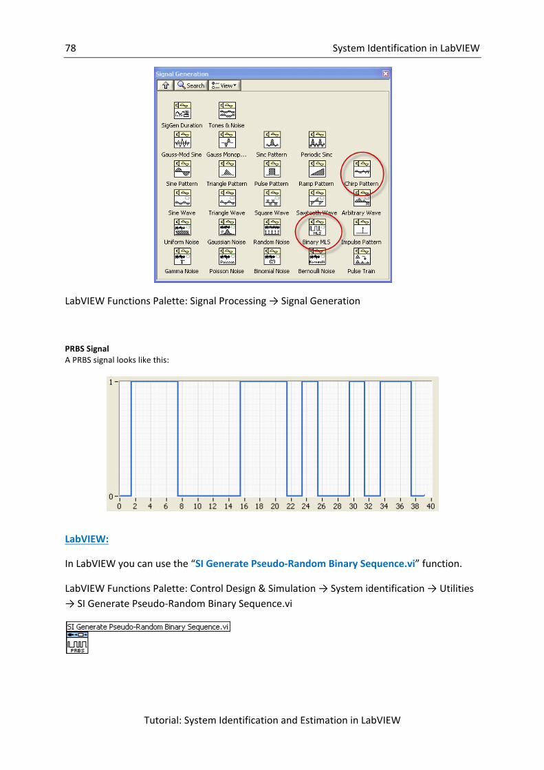
78 SystemIdentificationinLabVIEW
Tutorial:SystemIdentificationandEstimationinLabVIEW
LabVIEWFunctionsPalette:SignalProcessing→SignalGeneration
PRBSSignalAPRBSsignallookslikethis:
LabVIEW:
InLabVIEWyoucanusethe“SIGeneratePseudo-RandomBinarySequence.vi”function.
LabVIEWFunctionsPalette:ControlDesign&Simulation→Systemidentification→Utilities→SIGeneratePseudo-RandomBinarySequence.vi
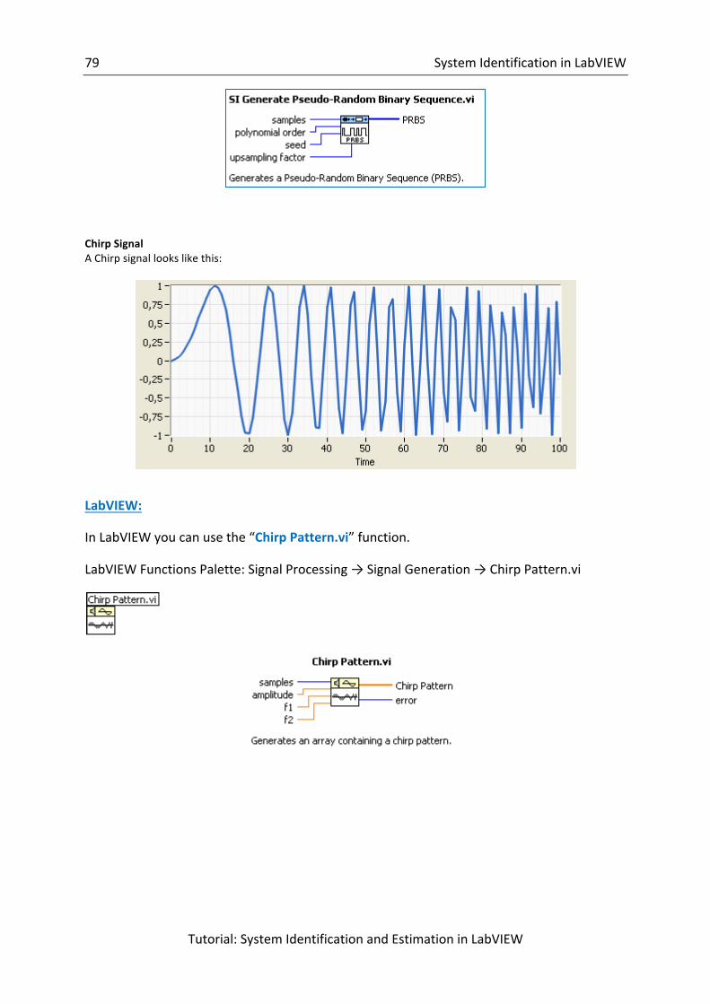
79 SystemIdentificationinLabVIEW
Tutorial:SystemIdentificationandEstimationinLabVIEW
ChirpSignalAChirpsignallookslikethis:
LabVIEW:
InLabVIEWyoucanusethe“ChirpPattern.vi”function.
LabVIEWFunctionsPalette:SignalProcessing→SignalGeneration→ChirpPattern.vi

80
11 OverviewofSystemIdentificationfunctions
InLabVIEWwecanusetheSystemIdentificationToolkit.
The“SystemIdentification”paletteinLabVIEW:
→UsetheSystemIdentificationVIstocreateandestimatemathematicalmodelsofdynamicsystems.YoucanusetheVIstoestimateaccuratemodelsofsystemsbasedonobservedinput-outputdata.
The“SystemIdentification”paletteinLabVIEWhasthefollowingsubpalettes:
Icon Name Description
Preprocessing
DataPreprocessing
UsetheDataPreprocessingVIstopreprocesstherawdatathatyouacquiredfromanunknownsystem.

81 OverviewofSystemIdentificationfunctions
Tutorial:SystemIdentificationandEstimationinLabVIEW
Parametric
ParametricModelEstimation
UsetheParametricModelEstimationVIstoestimateaparametricmathematicalmodelforanunknown,linear,time-invariantsystem.
Frequency
Frequency-DomainModelEstimation
UsetheFrequency-DomainModelEstimationVIstoestimatethefrequencyresponsefunction(FRF)andtoidentifyatransferfunction(TF)orastate-space(SS)modelofanunknownsystem.
Grey-Box
PartiallyKnownModelEstimation
UsethePartiallyKnownModelEstimationVIstocreateandestimatepartiallyknownmodelsfortheplantinasystem.
Recursive
RecursiveModelEstimation
UsetheRecursiveModelEstimationVIstorecursivelyestimatetheparametricmathematicalmodelforanunknownsystem.
Nonparametric
NonparametricModelEstimation
UsetheNonparametricModelEstimationVIstoestimatetheimpulseresponseorfrequencyresponseofanunknown,linear,time-invariantsystemfromaninputandcorrespondingoutputsignal.
Validation
ModelValidation
UsetheModelValidationVIstoanalyzeandvalidateasystemmodel.
Analysis
ModelAnalysis
UsetheModelAnalysisVIstoperformaBode,Nyquist,orpole-zeroanalysisofasystemmodelandtocomputethestandarddeviationoftheresults.
Conversion
ModelConversion
UsetheModelConversionVIstoconvertmodelscreatedintheLabVIEWSystemIdentificationToolkitintomodelsyoucanusewiththeLabVIEWControlDesignandSimulationModule.YoucanconvertanAR,ARX,ARMAX,output-error,Box-Jenkins,general-linear,orstate-spacemodelintoatransferfunction,zero-pole-gain,orstate-spacemodel.Youalsocanconverta
82 OverviewofSystemIdentificationfunctions
Tutorial:SystemIdentificationandEstimationinLabVIEW
continuousmodeltoadiscretemodelorconvertadiscretemodeltoacontinuousmodel.
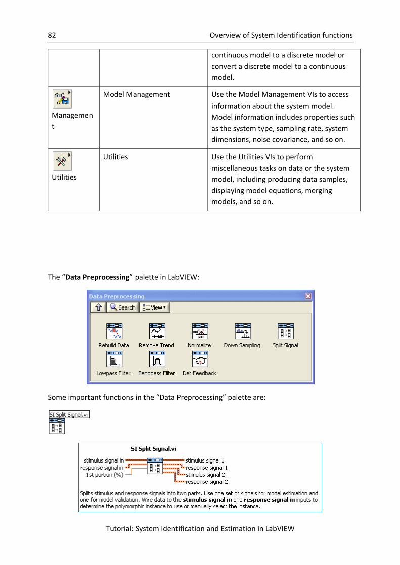
Management
ModelManagement
UsetheModelManagementVIstoaccessinformationaboutthesystemmodel.Modelinformationincludespropertiessuchasthesystemtype,samplingrate,systemdimensions,noisecovariance,andsoon.
Utilities
Utilities
UsetheUtilitiesVIstoperformmiscellaneoustasksondataorthesystemmodel,includingproducingdatasamples,displayingmodelequations,mergingmodels,andsoon.
The“DataPreprocessing”paletteinLabVIEW:
Someimportantfunctionsinthe“DataPreprocessing”paletteare:

83 OverviewofSystemIdentificationfunctions
Tutorial:SystemIdentificationandEstimationinLabVIEW
The“ParametricModelEstimation”paletteinLabVIEW:
Someimportantfunctionsinthe“ParametricModelEstimation”paletteare:
The“ParametricModelEstimation”paletteinLabVIEWhassubpalettefor“PolynomialModelEstimation”:

84 OverviewofSystemIdentificationfunctions
Tutorial:SystemIdentificationandEstimationinLabVIEW
→UsethePolynomialModelEstimationVIstoestimateanAR,ARX,ARMAX,Box-Jenkins,oroutput-errormodelforanunknown,linear,time-invariantsystem.
Someimportantfunctionsinthe“PolynomialModelEstimation”paletteare:
85
12 SystemIdentificationExampleWewanttoidentifythemodelofagivensystem.
Wehavefoundthemodeltobe:
𝑥 = −1𝑇𝑥 + 𝐾𝑢(𝑡 − 𝜏)
where
𝑇 isthetimeconstant
𝐾 isthesystemgain,e.g.pumpgain
𝜏 isthetime-delay
→Wewanttofindthemodelparameters 𝑇, 𝐾, 𝜏 usingtheLeastSquaremethod.WewilluseLabVIEWandMathScript.
Setthesystemontheform 𝒚 = 𝛗𝜽
Solutions:
Weget:
𝑥�= 𝑥 𝑢(𝑡 − 𝜏)
�
−1𝑇𝐾|
i.e.
𝜃 = −1𝑇𝐾
Inordertofind 𝜃 usingtheLeastSquaremethodweneedtologinputandoutputdata.Thismeansweneedtodiscretizethesystem.
WeuseasimpleEulerforwardmethod:
𝑥 ≈𝑥JK7 − 𝑥J
𝑇@
𝑇@ isthesamplingtime.

86 SystemIdentificationExample
Tutorial:SystemIdentificationandEstimationinLabVIEW
Thisgives:
𝑥JK7 − 𝑥J𝑇@�
= 𝑥J 𝑢J> ?�̀
�
−1𝑇𝐾|
Let’sassume 𝜏 = 3𝑠 (whichcanbefoundfromasimplestepresponseontherealsystem),wethenget(withsamplingtime 𝑇@ = 0.1):
𝑥JK7 − 𝑥J𝑇@�
= 𝑥J 𝑢J>�6�
−1𝑇𝐾|
Note!In3secondswelog30pointswithdatausingsamplingtime 𝑻𝒔 = 𝟎. 𝟏!!!
Giventhefollowingloggingdata(thedataisjustforillustrationandnotrealistic):
𝒌 𝒖 𝒚
1 0.9 3
2 1.0 4
3 1.1 5
4 1.2 6
5 1.3 7
6 1.4 8
7 1.5 9
Weusethefollowingsamplingtime: 𝑻𝒔 = 𝟏𝒔
Fromasimplestepresponse,wehavefoundthetime-delaytobe: 𝜏 = 3𝑠.
→Setthesystemontheform 𝒀 = 𝚽𝛉
Solutions:
Withtime-delay 𝜏 = 3𝑠and 𝑇@ = 1𝑠 weget:
87 SystemIdentificationExample
Tutorial:SystemIdentificationandEstimationinLabVIEW
𝑥JK7 − 𝑥J𝑇@�
= 𝑥J 𝑢J>��
−1𝑇𝐾|
Usingthegivendatasetwecansetontheform 𝑌 = Φθ:
7 − 68 − 79 − 8
=6 0.97 1.08 1.1
−1𝑇𝐾
i.e.:
111z
=6 0.97 1.08 1.1
{
−1𝑇𝐾|
Note!Weneedtomakesurethedimensionsarecorrect.
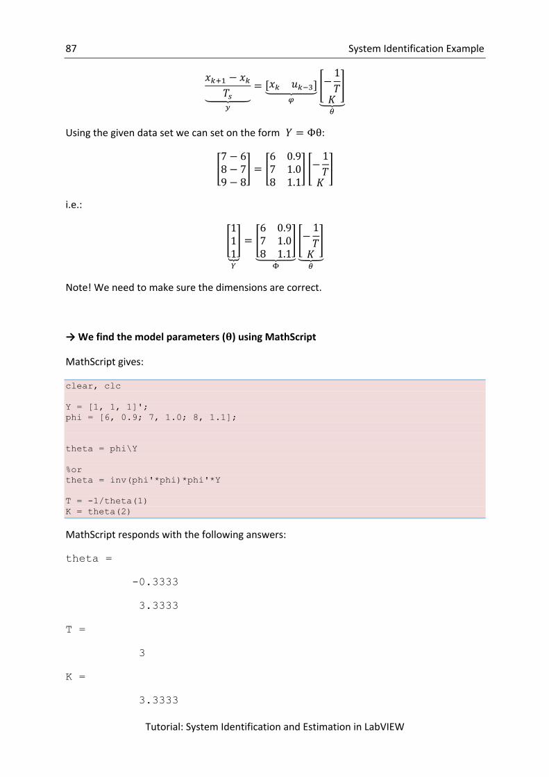
→Wefindthemodelparameters(𝛉)usingMathScript
MathScriptgives:
clear, clc Y = [1, 1, 1]'; phi = [6, 0.9; 7, 1.0; 8, 1.1]; theta = phi\Y %or theta = inv(phi'*phi)*phi'*Y T = -1/theta(1) K = theta(2)
MathScriptrespondswiththefollowinganswers:
theta =
-0.3333
3.3333
T =
3
K =
3.3333
88 SystemIdentificationExample
Tutorial:SystemIdentificationandEstimationinLabVIEW
i.e.,themodelparametersbecome:
𝑇 = 3, 𝐾 =103, 𝜏 = 3
Whichgivesthefollowingmodell:
𝑥 = −1𝑇𝑥 + 𝐾𝑢(𝑡 − 𝜏)
Withvalues:
𝑥 = −13𝑥 +
103(𝑡 − 3)
ImplementthemodelinLabVIEW.Use 𝑻 = 𝟓, 𝑲 = 𝟐, 𝝉 = 𝟑 andsimulatethesystem.Plotthestepresponseforthesystem.
Model:
𝑥 = −1𝑇𝑥 + 𝐾𝑢(𝑡 − 𝜏)
Where 𝑇 = 5, 𝐾 = 2, 𝜏 = 3
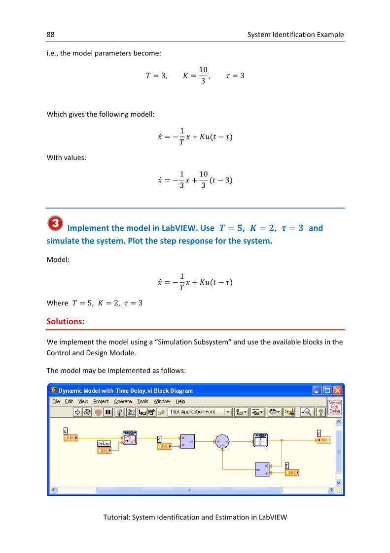
Solutions:
Weimplementthemodelusinga“SimulationSubsystem”andusetheavailableblocksintheControlandDesignModule.
Themodelmaybeimplementedasfollows:
89 SystemIdentificationExample
Tutorial:SystemIdentificationandEstimationinLabVIEW
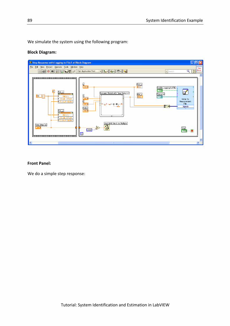
Wesimulatethesystemusingthefollowingprogram:
BlockDiagram:
FrontPanel:
Wedoasimplestepresponse:

90 SystemIdentificationExample
Tutorial:SystemIdentificationandEstimationinLabVIEW
Findthetransferfunctionforthesystem:
𝐻 𝑠 =𝑥(𝑠)𝑢(𝑠)
Model:
𝑥 = −1𝑇𝑥 + 𝐾𝑢(𝑡 − 𝜏)
PlotthestepresponseforthetransferfunctioninMathScript.Compareanddiscusstheresultsfromprevioustask.
Solutions:
Weusethedifferentialequation:
𝑥 = −1𝑇𝑥 + 𝐾𝑢(𝑡 − 𝜏)
Laplacetransformationgives:

91 SystemIdentificationExample
Tutorial:SystemIdentificationandEstimationinLabVIEW
𝑠𝑥(𝑠) = −1𝑇𝑥(𝑠) + 𝐾𝑢(𝑠)𝑒>?@
Note!WeusethefollowingLaplacetransformation:
𝐹 𝑠 𝑒>?@ ⟺ 𝑓(𝑡 − 𝜏)
𝑠𝐹(𝑠) ⟺ 𝑓(𝑡)
Thenweget:
𝑠𝑥 𝑠 +1𝑇𝑥 𝑠 = 𝐾𝑢(𝑠)𝑒>?@
and:
𝑥 𝑠 𝑠 +1𝑇
= 𝐾𝑢(𝑠)𝑒>?@
and:
𝑥 𝑠𝑢(𝑠)
=𝐾
𝑠 + 1𝑇𝑒>?@
Finally:
𝐻 𝑠 =𝑥 𝑠𝑢(𝑠)
=𝐾𝑇
𝑇𝑠 + 1𝑒>?@ =
𝐾���𝑇𝑠 + 1
𝑒>?@
Withvalues(𝑇 = 5, 𝐾 = 2, 𝜏 = 3):
𝐻 𝑠 =𝑥 𝑠𝑢(𝑠)
=10
5𝑠 + 1𝑒>�@
MathScript:
WeimplementthetransferfunctioninMathScriptandperformastepresponse.Weusethestep()function.
clear, clc s=tf('s'); K=2; T=5; H1=tf(K*T/(T*s+1)); delay=3; H2=set(H1,'inputdelay',delay); step(H2)
92 SystemIdentificationExample
Tutorial:SystemIdentificationandEstimationinLabVIEW
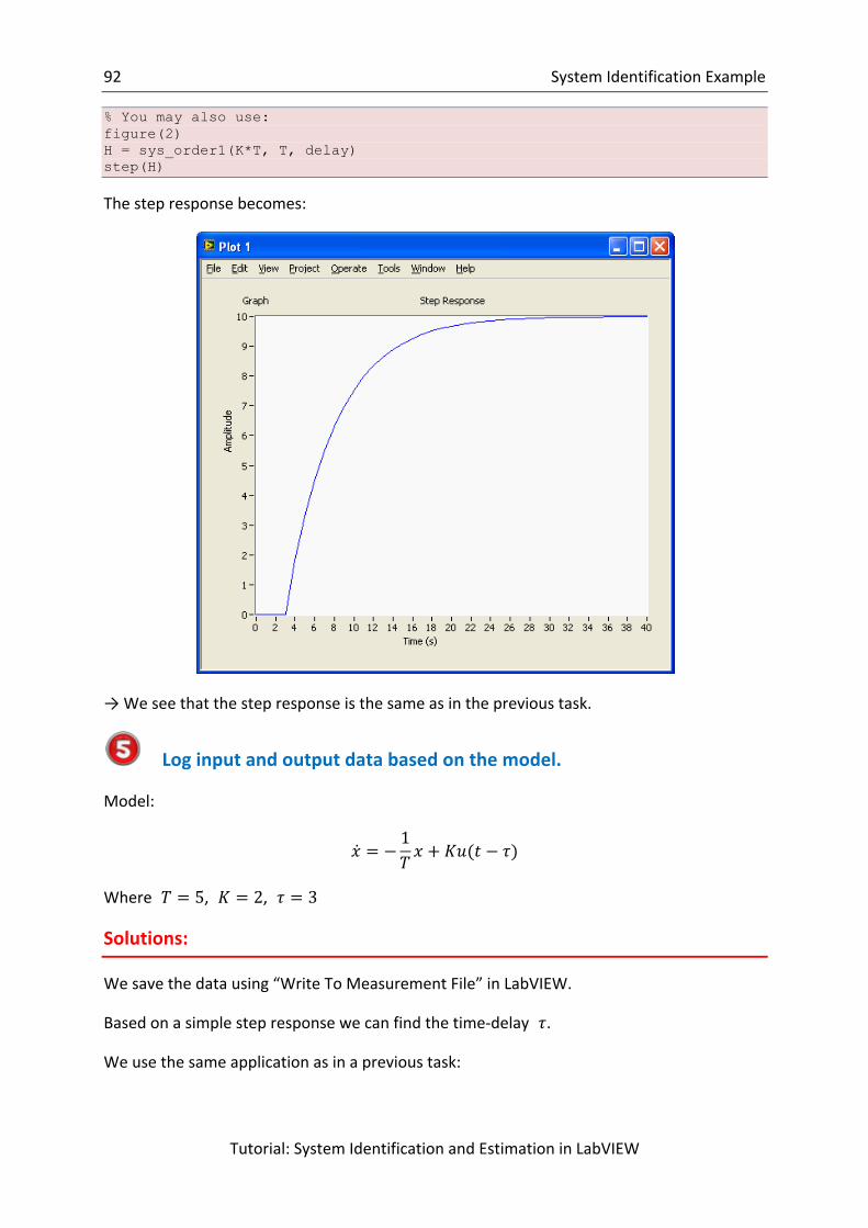
% You may also use: figure(2) H = sys_order1(K*T, T, delay) step(H)
Thestepresponsebecomes:
→Weseethatthestepresponseisthesameasintheprevioustask.
Loginputandoutputdatabasedonthemodel.
Model:
𝑥 = −1𝑇𝑥 + 𝐾𝑢(𝑡 − 𝜏)
Where 𝑇 = 5, 𝐾 = 2, 𝜏 = 3
Solutions:
Wesavethedatausing“WriteToMeasurementFile”inLabVIEW.
Basedonasimplestepresponsewecanfindthetime-delay 𝜏.
Weusethesameapplicationasinaprevioustask:
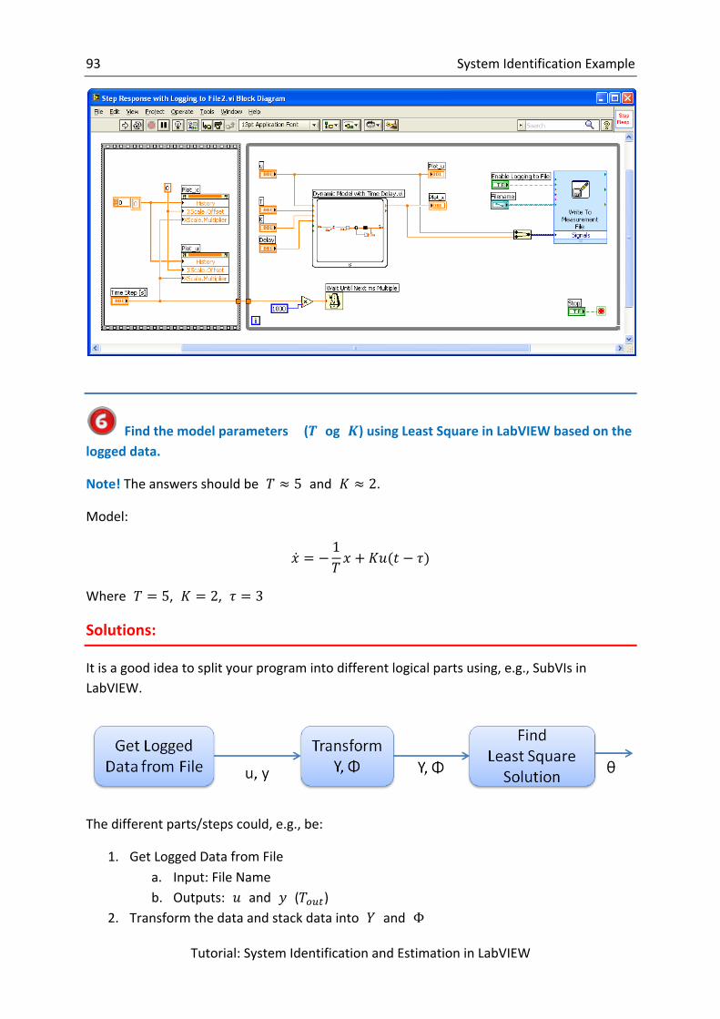
93 SystemIdentificationExample
Tutorial:SystemIdentificationandEstimationinLabVIEW
Findthemodelparameters (𝑻 og 𝑲)usingLeastSquareinLabVIEWbasedontheloggeddata.
Note!Theanswersshouldbe 𝑇 ≈ 5 and 𝐾 ≈ 2.
Model:
𝑥 = −1𝑇𝑥 + 𝐾𝑢(𝑡 − 𝜏)
Where 𝑇 = 5, 𝐾 = 2, 𝜏 = 3
Solutions:
Itisagoodideatosplityourprogramintodifferentlogicalpartsusing,e.g.,SubVIsinLabVIEW.
Thedifferentparts/stepscould,e.g.,be:
1. GetLoggedDatafromFilea. Input:FileNameb. Outputs: 𝑢 and 𝑦 (𝑇���)
2. Transformthedataandstackdatainto 𝑌 and Φ
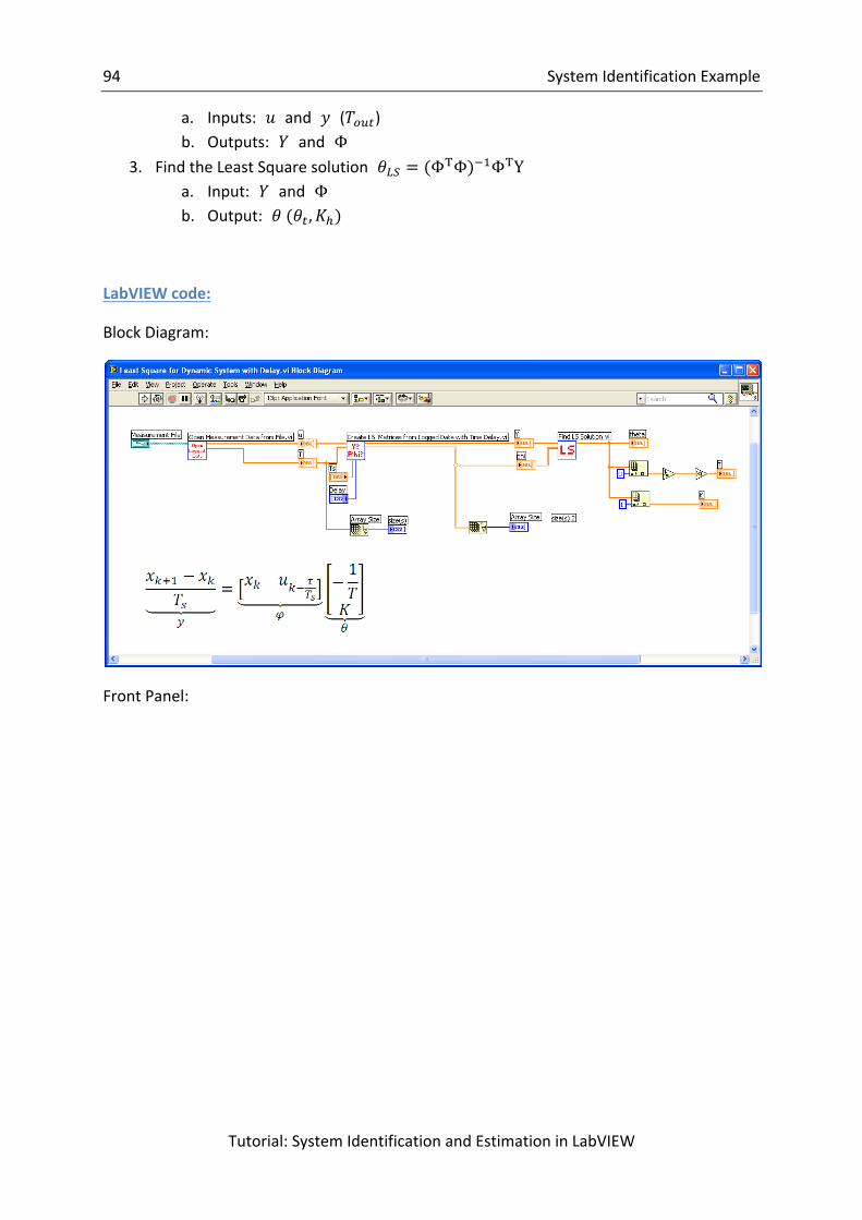
94 SystemIdentificationExample
Tutorial:SystemIdentificationandEstimationinLabVIEW
a. Inputs: 𝑢 and 𝑦 (𝑇���)b. Outputs: 𝑌 and Φ
3. FindtheLeastSquaresolution 𝜃st = (ΦuΦ)>7ΦuYa. Input: 𝑌 and Φb. Output: 𝜃(𝜃�, 𝐾�)
LabVIEWcode:
BlockDiagram:
FrontPanel:
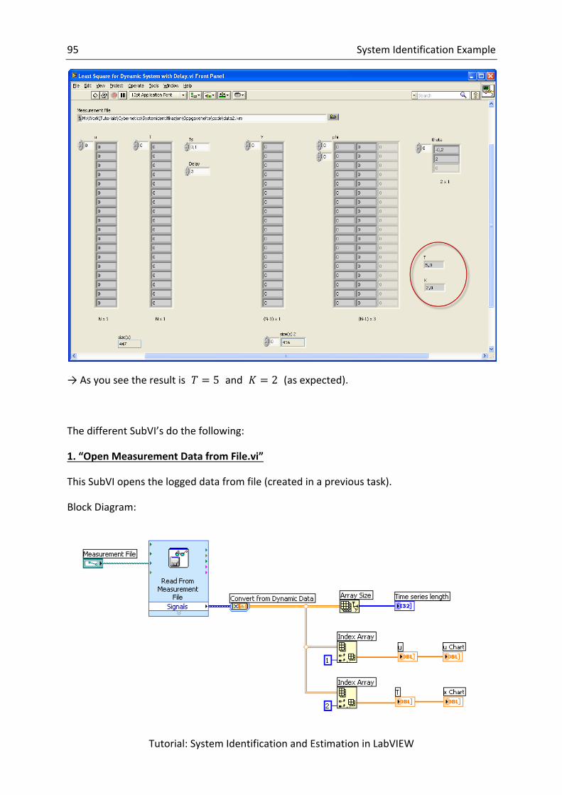
95 SystemIdentificationExample
Tutorial:SystemIdentificationandEstimationinLabVIEW
→Asyouseetheresultis 𝑇 = 5 and 𝐾 = 2 (asexpected).
ThedifferentSubVI’sdothefollowing:
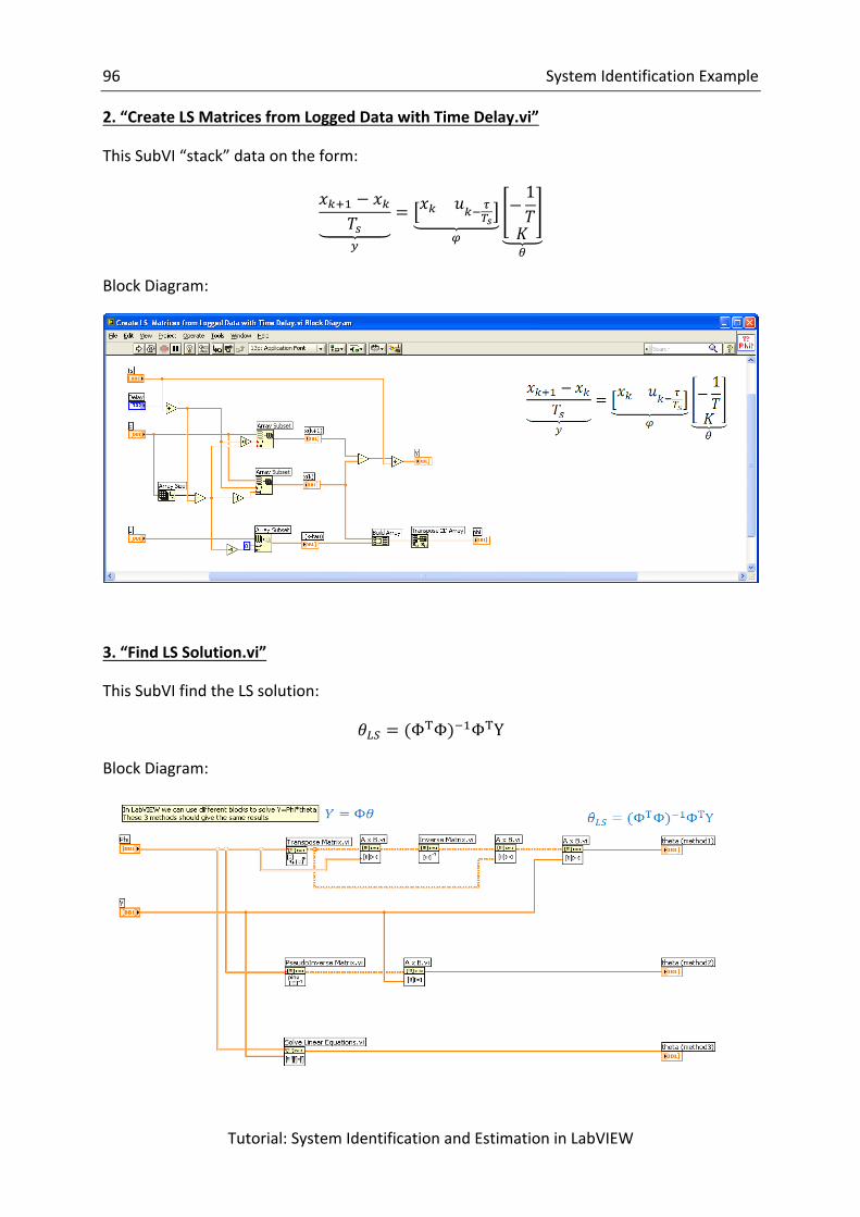
1.“OpenMeasurementDatafromFile.vi”
ThisSubVIopenstheloggeddatafromfile(createdinaprevioustask).
BlockDiagram:
96 SystemIdentificationExample
Tutorial:SystemIdentificationandEstimationinLabVIEW
2.“CreateLSMatricesfromLoggedDatawithTimeDelay.vi”
ThisSubVI“stack”dataontheform:
𝑥JK7 − 𝑥J𝑇@�
= 𝑥J 𝑢J> ?�̀
�
−1𝑇𝐾|
BlockDiagram:
3.“FindLSSolution.vi”
ThisSubVIfindtheLSsolution:
𝜃st = (ΦuΦ)>7ΦuY
BlockDiagram:
SystemIdentificationandEstimationinLabVIEW
Hans-PetterHalvorsen
Copyright©2017
E-Mail:[email protected]
Web:https://www.halvorsen.blog
https://www.halvorsen.blog