SUPPLY CHAIN SALES PROMOTION:
THE OPERATIONS AND MARKETING INTERFACE
By
SHILEI YANG
A dissertation submitted in partial fulfillment of the requirements for the degree of
DOCTOR OF PHILOSOPHY
WASHINGTON STATE UNIVERSITY College of Business
AUGUST 2007
© Copyright by SHILEI YANG, 2007
All Rights Reserved

© Copyright by SHILEI YANG, 2007
All Rights Reserved

ii
To the Faculty of Washington State University:
The members of the Committee appointed to examine the dissertation
of SHILEI YANG find it satisfactory and recommend that it be accepted.
___________________________________ Chair ___________________________________ ___________________________________ ___________________________________

iii
ACKNOWLEDGMENT
I am deeply indebted to my advisor, Charles L. Munson, who committed himself
to my development from the day I arrived in the program. This dissertation would not
have been possible without his sincere encouragement and wise guidance. I am also
indebted to Bintong Chen for his valuable support in pursuing the research topics and
his constructive comments on my dissertation. I am also blessed with the expertise of
my other committee members Pratim Datta and David E. Sprott. I deeply appreciate
their generous support and commitment to my dissertation work.
I would also like to acknowledge the financial support and facilities that were
graciously provided by the Department of Management and Operations during my
four-year process as a doctoral student. Finally, I would like to thank my big family,
all my previous teachers and many wonderful friends for their encouragement in this
long journey to pursue a doctoral degree.

iv
INCENTIVES OF THE DISSERTATION
With the widespread use of business models in practice, traditional operational
decisions have been integrated with other types of decisions, such as pricing,
promotions, system design, etc. For any firm, previous myopic cost control
operational decision making must be shifted to a multi-dimensional decision making
process. It seems natural for us to understand the how operational area interacts with
other functional areas.
In academia, focused disciplinary research has been the traditional approach for
each individual functional area (e.g., operations, marketing, information systems, and
finance). In the past decade, however, interdisciplinary research across functional
areas has become a very active research stream. By applying newly acquired
knowledge from other functional areas to my specifically trained area, I believe this
fusion of ideas can certainly improve our understanding of operations management
and hopefully generate more managerial insights for decision making in industry.

v
SUPPLY CHAIN SALES PROMOTION:
THE OPERATIONS AND MARKETING INTERFACE
Abstract
By Shilei Yang, Ph.D. Washington State University
August 2007
Chair: Charles L. Munson
Supply chain sales promotion is critical to the organizations in the channel due to
complications with hooking up manufacturers, retailers and consumers together. This
dissertation analyzes models discussing supply chain sales promotion under
collaboration between the operations and marketing disciplines. Borrowing from the
marketing empirical research on consumers’ slippage behavior, this research focuses
on the optimal use of mail-in rebate promotions in conjunction with other promotional
tools to maximized supply chain profits.
Related literature is organized in Chapter 2. Following the literature review are
three independent modeling chapters. Chapter 3 uses a utility function approach to
study the manufacturer’s profitability with two promotional strategies: rebates and

vi
manufacturer’s suggested retail prices (MSRP). The results show that the
manufacturer’s optimal strategies are jointly determined by the slippage rate and
magnitude of loss aversion. Chapter 4 uses a newsvendor modeling framework to
study coordinating issues between the manufacturer and the retailer when the
manufacturer provides rebates to consumers and the retailer exerts promotional effort
to further spur demand. The results show that a quantity discount contract is enough
to coordinate a supply chain under a typical deterministic demand model. For
stochastic demand, a quantity discount contract plus buy-back can coordinate the
supply chain. Chapter 5 uses an economic order quantity (EOQ) modeling
framework to study the retailer’s choices of promotional strategies: rebate promotions
or everyday low prices. The results show that the retailer’s decision making depends
upon several important factors including the demand price sensitivity and the regular
undiscounted retail price on market.
These research results provide insights for both operations managers and
marketers to facilitate proper choosing and designing of sales promotions over a
supply chain. Furthermore, scholars interested in cross-disciplinary studies between
operations and marketing can utilize the work here as a springboard to explore a wide
range of future applications.
vii
TABLE OF CONTENTS
Page
ACKNOWLEDGMENT……………………………………………………… INCENTIVES OF THE DISSERTATION…………………………………… ABSTRACT…………………………………………………………………… LIST OF TABLES…………………………………………………………… LIST OF FIGURES…………………………………………………………… CHAPTER 1. INTRODUCTION………………………………………..……………… 2. LITERATURE REVIEW………………………………………..…………
Sales promotion…………………………………………………………… Rebates…………………………………………………………..………… Pricing and production/inventory interface...………………..…………… Supply chain/channel.……………………………………………………… Contractual coordination…………………………………………………… Summary………………………………………………………..…………
3. CHANNEL ANALYSIS OF REBATE PROMOTION WITH REFERENCE-DEPENDENT CONSUMERS…………………………… Introduction……………………………………………………………… Model environment……………………………………………………… Model with rebate promotion only………………………………………… Reference-dependent model with rebate promotion……………………… Reference-dependent but loss-neutral model with rebate promotion……… Integrated channel with rebate promotion………………………………… Channel performance with rebate promotion……………………………… Numerical studies………………………………………………………… Conclusions………………………………………………………………..
4. COORDINATING CONTRACTS UNDER SALES PROMOTION..……
Introduction……………………………………………………………… Model development……………………………………………………… The deterministic demand model…………………………………………
Quantity discount contract……………………………………… Two-part tariff contract…………………………………………
The stochastic demand model…………………………………………… Centralized supply chain………………………………………… Buy-back only contract………………………………………………
iii iv v ix x 1 7 8 13 18 21 24 30
33 34 36 40 42 47 49 51 53 54
66 67 69 73 73 77 78 79 81
viii
Continuous quantity discount contract with buy-back……………… Discrete quantity discount contract with buy-back…………………
Numerical studies………………………………………………………… Conclusions………………………………………………………………..
5. RETAILER’S PROMOTIONAL CAMPAIGN: WHY WAL-MART
NEVER ISSUES REBATE ……………….………………….…….……. Introduction……………………………………………………………… Model development……………………………………………………… Analysis of rebate promotions using specific functional forms…………… Analysis of EDLP policy………………………………………………… Sensitivity analysis and discussions……………………………………… Comparative example……………………………………………………… Conclusions………………………………………………………………..
APPENDIX
Proof of Proposition 3.1. ………………………………………………… Proof of Lemma 3.1. ……………………………………………………… Proof of Proposition 3.2…………………………………………………… Proof of Proposition 3.4…………………………………………………… Proof of Lemma 4.1. ……………………………………………………… Proof of Theorem 4.4……………………………………………………… Proof of Lemma 4.2. ……………………………………………………… Proof of Theorem 4.5……………………………………………………… Proof of Theorem 4.6………………………………………………………
LIST OF REFERENCES
84 86 91 94
100 101 102 106 109 110 114 115
123 124 127 131 139 147 148 149 150 151
156

ix
LIST OF TABLES
Page 1 INTRODUCTION
1.1 Specific sales promotion tools……………………………………… 2 LITERATURE REVIEW
2.1 Popular contract forms……………………………………………… 2.2 Summary of most relevant literature………………………………
3 CHANNEL ANALYSIS OF REBATE PROMOTION WITH
REFERENCE-DEPENDENT CONSUMERS 3.1 The equilibrium solution of rebate promotion only without slippage. 3.2 The equilibrium solution of rebate promotion only with slippage… 3.3 The equilibrium solution sets of reference-dependent model.……… 3.4 The equilibrium solution sets of loss-neutral model……………… 3.5 The equilibrium solution sets of integrated channel………………
4 COORDINATING CONTRACTS UNDER SALES PROMOTIONS
5 PROMOTIONAL CAMPAIGN 5.1 Effects of price sensitivity parameter b…………………………… 5.2 Optimal solutions of the comparative example……………………..
APPENDIX A.1. The candidate solution sets in decentralized channel………………
A.2. The candidate solution sets in integrated channel….. ………………
6
31 32
62 62 63 64 65
122 122
154 155
x
LIST OF FIGURES
Page 1 INTRODUCTION
1.1 A schematic framework of the supply chain………………………… 1.2 A schematic framework of the types of promotion…………………… 1.3 A schematic framework of the dissertation work………………………
2 LITERATURE REVIEW 3 CHANNEL ANALYSIS OF REBATE PROMOTION WITH
REFERENCE-DEPENDENT CONSUMERS 3.1 An MSRP example…………………………………….……………… 3.2 A schematic framework of the market environment ………………… 3.3 The kinked demand curve………….…………….... ………………… 3.4 A schematic framework of reference-dependent model……………… 3.5 A schematic framework of loss-neutral model…….... ……………… 3.6 A schematic framework of integrated channel ….... ………………… 3.7 A numerical example ….... ……………………………………………
3.8 The joint effects of s or r and β on the manufacturer’s profit.……
4 COORDINATING CONTRACTS UNDER SALES PROMOTIONS
4.1 An example of restricted rebates promotion………………………… 4.2 The layout of proposed contracts…….…………….... ……………… 4.3 Numerical examples of contract efficiency………….………………… 4.4 Sensitivity analysis one………….…………….... …………………… 4.5 Sensitivity analysis two.. ………………………………………………
5 PROMOTIONAL CAMPAIGN
5.1 Price sensitivity parameter b vs profits…………………………….… 5.2 Market potential parameter a vs profits………….……………….…… 5.3 Market potential parameter a vs optimal rebate value……………. … 5.4 Regular retail price vs profits. ………………………………………… 5.5 Regular retail price vs optimal rebate value…….... ………………… 5.6 The joint effects of regular retail price and price sensitivity ………… 5.7 Rebate costliness c vs optimal rebate value…….... ………………… 5.8 Rebate costliness c vs optimal redemption effort level….... …………
APPENDIX A.1. The manufacturer’s candidate strategy sets in decentralized channel…
A.2. The manufacturer’s candidate strategy sets in integrated channel……..
5 5 5
57 57 58 59 59 59 60 61
96 96 97 98 99
118 118 119 119 120 120 121 121
153 153
xi
Dedication
This dissertation is dedicated to my grandmother and parents.

- 1 -
CHAPTER 1
INTRODUCTION

- 2 -
Over the past decade, emerging business technologies have provided new
opportunities for enhancing the collaboration between marketing and operations. Both
practitioners and researchers have increased their focus on the management of the
interface between marketing and operations.
Classic operational decisions involve production, procurement and inventory
decisions; while classic marketing decisions involve pricing, advertising, promotional
decisions. These kinds of decisions making can either be the activities of a single firm
or between multiple business entities. The decision making for coordinating different
business entities, i.e., manufacturers and retailers, falls within the realm of supply
chain management. In the operations literature, supply chain management is called
“the tactical and strategic control of network of firms from raw materials to finished
goods” (Cachon 2006). Below is a figure of the typical supply chain.
[Insert Figure 1.1. here]
However, in the marketing literature, the term “supply chain” has been noticeably
replaced by another term, “marketing channel”, which refers to “the set of
interdependent organizations involved in taking a product or service from its point of
production to its point of consumption” (Iyer and Padmanabhan 2003). Although there
is no major distinction between the definitions of these two terms, marketers use the
word “consumption” to indicate their special focus on consumers, i.e., all marketing
events should have an impact on final consumers.

- 3 -
In this dissertation, the consumers’ behavior has been embedded into sales promotion.
More specifically, I incorporate sales promotion into the study of a supply chain. As a
ubiquitous component of marketing mix, sales promotion can be defined as “an
action-focused marketing event whose purpose is to have a direct impact on the
behavior of the firm’s customers” (Blattberg and Neslin 1990). A traditional but more
thorough definition of sales promotion is offered by Ulanoff (1985):
Sales promotion consists of all the marketing and promotion activities, other than
advertising, personal selling, and publicity, that motivate and encourages the
consumer to purchase, by means of such inducements as premiums, advertising
specialties, samples, cents-off coupons, sweepstakes, contests, games, trading stamps,
refunds, rebates, exhibits, displays, and demonstrations. It is employed, as well, to
motivate retailers’, wholesalers’, and manufacturers’ sales forces to sell, through the
use of such incentives as awards or prizes (merchandise, cash, and travel), direct
payments and allowances, cooperative advertising, and trade shows.
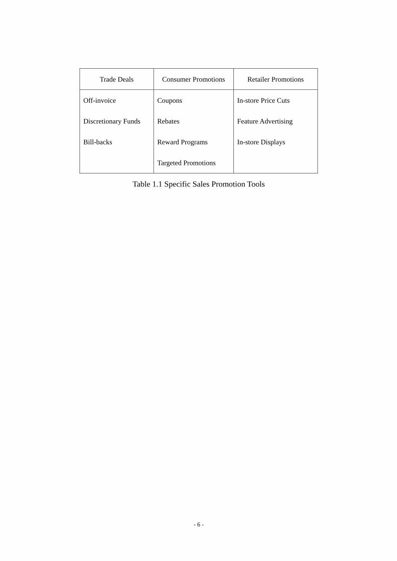
There are three major types of sales promotion: trade deals, retailer promotions, and
consumer promotions. Strategically, trade deals and retailer promotions are elements
of the push effort, while consumer promotions offered by the manufacturers are part
of the pull effort. As Figure 1.2 demonstrates, by including the pull effort, I
successfully complete a closed loop in the supply chain.
[Insert Figure 1.2. here]
For each type of promotion, a variety of special promotional tools exists. Table 1.1
lists out the most discussed tools in the marketing literature (Neslin, 2002).

- 4 -
[Insert Table 1.1. here]
In this dissertation, I focus on rebates (i.e., mail-in rebates) as the representative of
consumer promotion. (Coupons can be shown to be a special case of rebates in my
models.) Retail promotion in my work is characterized into a more general form:
retailer promotional effort (more detailed discussion provided in the literature review
section). Trade deals between manufacturers and retailers in my work involve
wholesale pricing, bill-backs (i.e., channel rebates or retailer rebates in the operations
literature), discretionary funds, and possibly some other techniques from the
operations literature, for example, buy-back, quantity discount, revenue sharing.
There are three independent modeling sections in this dissertation. In the first section,
I use a utility-based model to study consumers’ behavior towards the interaction of
rebates and reference price. In the second section, I develop coordinating contracts
between trading partners under all three types of sales promotions. In the last section,
I compare two types of common retailing strategies, everyday low pricing and rebate
promotional pricing, in the category of single-firm decision making. The following
figure describes my dissertation framework.
[Insert Figure 1.3. here]

- 5 -
Figure 1.1 A Schematic Framework of the Supply Chain
Figure 1.2 A Schematic Framework of the Types of Promotion
Figure 1.3 A Schematic Framework of the Dissertation Work
Trade Deals Manufacturer Retailer
Consumer
Consumer Promotions
Retailer Promotions
Manufacturer Retailer Consumer
- 6 -
Trade Deals Consumer Promotions Retailer Promotions
Off-invoice
Discretionary Funds
Bill-backs
Coupons
Rebates
Reward Programs
Targeted Promotions
In-store Price Cuts
Feature Advertising
In-store Displays
Table 1.1 Specific Sales Promotion Tools

- 7 -
CHAPTER 2
LITERATURE REVIEW

- 8 -
2.1. Sales Promotion
Sales promotion is certainly the most important element of marketing mix. Statistics
for packaged goods companies show that sales promotion comprises nearly 75% of
the marketing budget (Neslin 2002). The marketing literature on sales promotion is
saturated with both theoretical and empirical works (see Blattberg and Nelsin 1990 for
the early work on sales promotion, Nelsin 2002 for an excellent recent review, and
Blattberg et al. 1995 for a summary of empirical generalization of promotions).
Consumers represent the ultimate targets of all promotions. Numerous marketing
articles focus on how sales promotion impacts the behavior of consumers, particularly
their purchasing decisions. For example, Neslin et al. (1985) studies the relationship
between consumer promotions and the acceleration of product purchases. Purchase
acceleration can behave in two ways: larger purchase quantities and shorter
interpurchase times. The authors estimate acceleration effects in two product
categories, and they conclude that featured advertising on price cuts is the most
effective tool for accelerating purchases. In a recent paper, Zhang et al. (2000)
compare two types of promotional incentives: immediate value incentives versus
delayed value incentives. They show that delayed incentives are more profitable in
markets where consumers exhibit high variety-seeking, while immediate incentives
are more profitable in markets where consumers exhibit inertia-proneness.
Among a variety of consumer behavior related topics, the phenomenon of reference

- 9 -
price has been a popular topic in marking literature. The reference price effect is
based on adaptation level, which is “determined by previous and current stimulus to
which a person has been exposed” (Blattberg and Neslin 1990). Consumers judge the
current available price by comparing it to the adaptation level, which is called
reference price. The utility from comparing purchase price relative to the reference
price is called transaction utility, or deal value. As a counterpart of transaction utility,
acquisition utility is the value derived from the intrinsic utility provided by an item,
relative to its purchase price (Neslin, 2002). So the total value of a transaction to a
consumer is the sum of acquisition utility and transaction utility. The support for the
existence of the reference price effect can be found in a variety of empirical studies
(see Kalyanaram and Winer 1995 for a review). Sometimes, however, consistent price
promotions may lower the reference prices of consumers, rendering future promotions
ineffective. Greenleaf (1995) shows that reference price effects can make the
promotion profitable if the profit gains in the current period exceed the losses in the
future. The author also proposes a recurring promotion model with dynamic
programming to identify the optimal promotional strategy in multiple periods.
There are two broad types of reference prices (Mayhew and Winer 1992): internal and
external reference prices. The internal ones are prices stored in the minds of
consumers and not presented in the physical environment, such as a historical price,
the lowest currently available price, or expected future price. External reference prices
are provided by observed stimuli in the purchase environment, such as the regular
- 10 -
price or suggested price displayed on sale tags or featured advertising. Most of the
existing literature has focused on internal reference price.
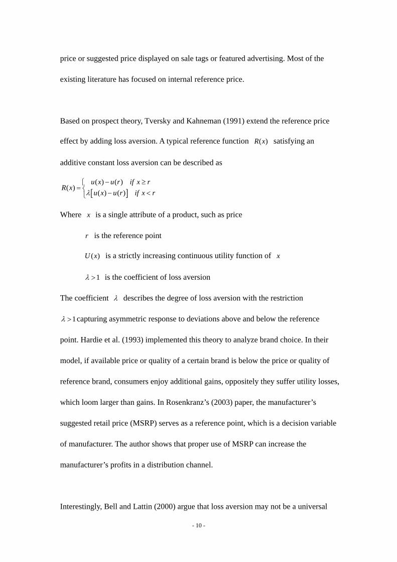
Based on prospect theory, Tversky and Kahneman (1991) extend the reference price
effect by adding loss aversion. A typical reference function ( )R x satisfying an
additive constant loss aversion can be described as
[ ]( ) ( )
( )( ) ( )
u x u r if x rR x
u x u r if x rλ− ≥⎧
= ⎨ − <⎩
Where x is a single attribute of a product, such as price
r is the reference point
( )U x is a strictly increasing continuous utility function of x
1λ > is the coefficient of loss aversion
The coefficient λ describes the degree of loss aversion with the restriction
1λ > capturing asymmetric response to deviations above and below the reference
point. Hardie et al. (1993) implemented this theory to analyze brand choice. In their
model, if available price or quality of a certain brand is below the price or quality of
reference brand, consumers enjoy additional gains, oppositely they suffer utility losses,
which loom larger than gains. In Rosenkranz’s (2003) paper, the manufacturer’s
suggested retail price (MSRP) serves as a reference point, which is a decision variable
of manufacturer. The author shows that proper use of MSRP can increase the
manufacturer’s profits in a distribution channel.
Interestingly, Bell and Lattin (2000) argue that loss aversion may not be a universal

- 11 -
phenomenon due to consumer price responsive heterogeneity. A more
price-responsive consumer has a lower price level as a reference point, while a less
price-responsive consumer tends to have a higher reference level. The authors show
that after controlling for heterogeneity in price responsiveness, the loss aversion effect
is no longer statistically significant. A recent empirical paper by Novemsky and
Kahneman (2005) also claims that loss aversion is not ubiquitous and that it has
certain boundaries. The authors propose that goods that are exchanged as intended do
not exhibit a loss aversion effect.
To address complex consumer behaviors, retailers generally employ one of two
different types of pricing strategies: everyday low pricing (EDLP) and promotional
pricing (HI/LO). EDLP does not necessarily imply no promotions at all, but EDLP
stores promote less frequently and less steeply than HI/LO stores. Marketing
researchers have postulated a variety of reasons for the coexistence of EDLP and
HI/LO. For example, EDLP stores appeal to “expected price shoppers”, while HI/LO
stores appeal to “cherry-pickers” (Lattin and Ortmeyer 1991). Moreover, EDLP stores
appeal to “large basket” shoppers, while HI/LO stores appeal to “small basket”
shoppers (David and Lattin 1998). Ho et al. (199) find that a rational shopper tends to
shop more often but purchase fewer quantities per visit at HI/LO stores. Other
researchers (Hoch et al. 1994, Lal and Rao 1997) argue that EDLP and HI/LO are
position strategies rather than merely pricing strategies.
- 12 -
The marketing research on retailer promotions or consumer promotions, like that
described above, focuses on consumers but ignores intra-firm issues between channel
members. Articles on trade promotions need to study the coordination between
manufacturers and retailers. As the most important element in promotional mix, trade
promotions command half of the marketing budget for many packaged goods firms
(Neslin 2002). In spite of the large amount of money spent on trade promotions, the
inefficiency of trade deals is a primary concern among manufacturers. The
inefficiency of trade promotions are usually attributed to two retailer behaviors:
passthrough and forward buying. Manufacturers offer trade promotions to retailers to
encourage them to reduce retail prices and, hence, generate incremental sales.
However, the retailers may decide not to pass through the full discount to consumers,
or they may forward buy the items by carrying inventory to satisfy future demand.
Much existing literature in trade promotions focuses on implementing proper
strategies or designing efficient tools to help manufacturers to alleviate the
passthrough and forward buying problems. For example, Dreze and Bell (2003)
suggest that manufacturers can redesign the scan-back deals to leave the retailers
weakly better off while leaving themselves strictly better off. Ault et al. (2000) show
that the strategic use of instant consumer rebates can increase manufacturers’ profits
caysed by mitigating arbitrage by retailers’ forward buying behavior. Kumar et al.
(2001) examine how consumer knowledge of trade promotions affect retailers’
passthrough behavior, and they suggest that manufacturers can advertise their trade
promotions directly to consumers, thus making consumers aware of the ongoing trade

- 13 -
deals. On the other hand, Lal et al. (1996) argue that forward buying has certain
benefits – for example, it can decrease the intensity of competition between
manufacturers. The authors explains that the forward buying makes the best trade
deals unprofitable to manufacturers while making the worst trade deals unacceptable
to retailers, consequently decreasing the overall probability of offering trade deals.
2.2. Rebates
This section reviews the literature on rebates, which represent the key element in this
dissertation work. In the chapters that follow, rebates exclusively represent
consumers’ mail-in rebates, and the redemption process typically requires consumers
to perform arduous tasks (filling forms, clipping labels and sending them via the mail).
In many papers, rebates have been modeled interchangeably with coupons (i.e.,
instant rebates). Although in many regards, rebates and coupons are similar (such as
sales impact, price discrimination, etc.), one fundamental difference is that coupons
are redeemed at the time of purchase and provide an immediate price reduction while
rebates can only be redeemed after purchasing the product at the regular price.
Couponing is the most researched form of consumer promotion by far (see Blattberg
and Nelsin 1990 p279 for a summary of couponing objectives). As the twin brother of
coupons, consumer promotion by rebates does not have much veritable research
(Neslin 2002), despite the fact that mail-in rebate business is increasing and the use of
traditional cents-off coupons is declining (Bulkeley 1998). In 2005, the total face
- 14 -
value of rebates is estimated to be $6 billion in the U.S. (Grow 2005).
The most fascinating phenomenon of rebates is consumers’ slippage behavior, which
occurs when “consumers are enticed to purchase as a result of a rebate offer but
subsequently fail to apply for the rebate” (Silk 2004). Business Week (Grow, 2005)
reports that “fully 40% of all rebates never get redeemed”, which gives rebate issuers
a large enough “arbitrage” space. Because this “arbitrage” space is so large, the
respective market shares of some companies have even increased by issuing rebates
(Bulkeley 1998). Most of the existing marketing literature on rebates can be generally
classified into two categories: WHY questions and HOW questions, i.e., explanation
for the phenomenon of slippage based on consumers’ responses to rebates, and the
influences of slippage on promotional strategies. Several early articles (Jolson et al.
1987, Tat et al. 1988) offer some initial explanation for the popularity of rebates.
Folkes and Wheat (1995) provide an interesting finding that consumer’s future price
expectations for products with rebates are higher than those with sales or coupons.
Soman (1998) suggests that consumer’s purchase decisions of products offering a
delayed incentive can be independent of the decisions to redeem the delayed incentive
itself. Purchase decisions are influenced by the face value of rebate offer; conversely,
redemption decisions are directly dependent on the extent of effort involved. The
author further shows that consumers usually underestimate their future effort needed
for rebate redemption. Gourville and Soman (2004) offer further insights into the
effort-discounting process with an anchoring and adjustment model. Chen et al. (2005)

- 15 -
argue that slippage can be attributed to the different post-purchase states of a
consumer. Gilpatric (2005) uses a present-biased preference model to explain the term
slippage.
Primarily based on Soman’s research, Silk (2004) suggest that there are three
characteristics of a rebate offer: value of the reward, length of the redemption period,
and redemption effort. Changes in any of these three characteristics have the potential
to influence both purchase and redemption. The author finds that the discrepancy
between consumers’ subjective probabilities of redeeming and their objective
probabilities of redeeming causes the slippage. The subjective probability of
redeeming represents a consumer’s redemption confidence at the time of purchase,
which is mainly determined by size of reward and length of redemption period. The
objective probability of redeeming represents a consumer’s actual redemption
behavior after purchase, which is influence by three post-purchase factors
(procrastination, prospective forgetting, and redemption effort). Another interesting
finding is that increasing the length of the redemption period can have a greater
impact on slippage than increasing the redemption effort. Silk and Janiszeweki (2004)
provide further support with industry surveys.
Recent analytical papers by quantitative marketing researchers have begun to address
how to take advantage of slippage behavior. Moorthy and Soman (2003) provide a
way to exacerbate the slippage effects by highlighting the reward and not highlighting

- 16 -
the effort required to redeem. Joseph and Kemieux (2005) explain how the
redemption cost influences the designing of rebate promotions. Moorthy and Lu (2004)
indicate that rebates are more efficient than coupons in price discriminating between
consumer types. Thompson and Noordewier (1992) use a time series approach to
study the problems of overusing cash rebates in the automobile industry. Besides the
slippage phenomenon, Dogan et al. (2005) show that rebate promotion can serve as an
effective market segmentation tool. The authors find that the disadvantaged firm tends
to pursue a segmentation strategy by offering rebates more frequently than the
advantaged one. Following these works by marketing researchers, operations
researchers have begun to apply rebate tools to supply chain management (described
in the next two sections).
Here, I list out the generalizations of rebates that can be drawn from literature by both
marketing and operations researchers. For each generalization, there are at least three
articles sharing the same results. Among them, the slippage phenomenon is uniquely
associated with rebates. Coupons may share the same findings (except slippage) with
rebates, although my synthesizing work is from the literature on rebates.

- 17 -
Price discriminating --- Gerstner and Hess (1991), Gerstner and Hess (1994), Moorthy and Lu
(2004), Chen et al. (2005), Joseph and Lemieux (2005).
Slippage/Breakage/Space-out phenomenon --- Bulkeley (1998), Grow (2005) Lieber (2005),
Mitchell (2005), Jolson et al. (1987), Silk and Janiszeweki (2004), Silk (2004), Chen et al.
(2005), Moorthy and Soman (2003), Moorthy and Lu (2004), Gilpatric (2005), Khouja
(2006): followed by some sub-findings
Redemption cost plays the critical role in designing rebates --- Soman (1998) Chen et al.
(2005), Joseph and Lemieux (2005).
Sales increase with rebate face value --- Soman (1998), Silk and Janiszeweki (2004),
Silk (2004).
Redemption rate decreases with redemption cost --- Tat et al. (1988), Khouja (2003),
Silk and Janiszeweki (2004).
The relationship between rebate face value and redemption rate is mixed --- Moorthy
and Lu (2004), Silk and Janiszeweki (2004) support a positive relationship; in contrast,
Soman (1998) and Silk (2004) argue that the effect of face value on redemption is weak.
Against forward-buying/inventory stock-up by retailer --- Bulkeley (1998), Ault et al. (2000),
Arcelus and Srinivasan (2003).
Improving the manufacturer’s profits and the channel profits --- Gerstner and Hess (1991),
Gerstner and Hess (1995), Chen et al., 2005 (2005), Aydin et al. (2005).
Increase retail price --- Gerstner and Hess (1991), Aydin et al. (2005), Arcelus et al. (2006);
however, Chen et al. (2005) argue that “the retailer may or may not increase its selling price
when the manufacturer offers a rebate”.

- 18 -
2.3. Pricing and Production/Inventory Interface
One major component of the marketing/operations interface is the integration of
operational decisions with retail pricing. This research area has also been called
marketing/manufacturing or pricing/inventory interface. The increased research in this
category coincides with the growth of the Internet and E-commerce, which has
opened up great opportunities for investigating the pricing mechanism. The latest
thorough reviews can be found in Yano and Gilbert (2003) and Chan et al. (2003).
Most of the articles in this category focus on decision making involving only a single
firm rather than on coordination issues within and between business entities. The firm
under investigation has control over production or inventory decisions, and the
price-sensitive demand is usually limited by the quantity produced or procured. The
firm’s goal is to align the incentives of marketing and production. This section
reviews the promotional related articles falling into this category. Although there are
many examples of promotional pricing in the marketing literature, operations
researchers have produced the majority of the work that aligns promotion decisions
with inventory or production decisions.
Sogomonian and Tang (1993) develop a multiple-period deterministic model to
maximize a firm’s net profit by choosing the timing and level of promotion, as well as
the level of production at each period. Their mixed-integer program results in a
"nested” longest path problem over a network, which can be solved in polynomial

- 19 -
time. Cheng and Sethi (1999) model a joint inventory-promotion decision problem for
a retailer. By using a Markov decision process, they find the optimal promotional
timing determined by an inventory threshold. If this threshold is exceeded, then the
retailer should promote the product. For the linear ordering cost case, they also find
that the retailer should replenish if the inventory falls below a certain base level.
Neslin et al. (1995) develop a model to maximize the manufacturer’s profits by
optimally allocating expenses on advertising directly to the consumers and offering
periodic trade deal discounts to the retailer.
Several recent papers on rebates can also be classified into this category. Two papers
(Arcelus et al. 2006 and Khouja 2003) use a newsvendor model to study the joint
pricing-inventory decision. In Arcelus et al.’s (2006) paper, a profit-maximizing
retailer needs to determine the optimal retail pricing and ordering policy when the
manufacturer offers the rebates directly to the consumers or a wholesale price
discount to the retailer itself. The authors analyze the retailer’s behavior through
two ratios: passthrough ratio and claw-back ratio (i.e., the proportion of
manufacturer’s rebates offset by the retail-price increase). In Khouja’s (2003) paper,
the expected profit for the manufacture is a function of three decision variables (retail
price, rebate face value, and the production quantity). The author shows that under
certain condition, offering rebates may lead to a large increase in the manufacturer’s
profit. In another paper, Khouja (2006) implements an EOQ-based model to jointly
consider the retailer’s optimal pricing, rebate value and lot sizing problems. The

- 20 -
author uses a simple linear deterministic demand function D a bP cR= − + , where the
ratio L c b= measures the effectiveness of a one-dollar increase in rebate face value
relative to a one-dollar drop in price. The author shows that an increase in the rebate
effectiveness leads to a larger optimal face value and greater profit.
This type of decision making is extended into a synchronized decision making of
marketing and operations departments within the same firm, which is called
“horizontal coordination”. When the two departments are in conflict, there is usually a
mismatch in demand and supply, leading to production inefficiencies and unsatisfied
consumers. Even when the two independent departments obtain their respective best
operating level, it may lead to a suboptimal performance of the firm as a whole. Based
on agency theory, Porteus and Whang (1991) suggest optimal compensation plans for
one manufacturing and multiple marketing managers. Hess and Lucas (2004) argue
that firms without initial knowledge of their potential customers should allocate
one-third of their resources to perform marketing research and the rest to manufacture
the goods. Pekgun et al. (2005) study a more complex case by adding leadtime. In
their paper, the marketing department chooses the price and the manufacturing
department chooses the lead time, where both variables influence the demand in a
linear way. The authors find that a transfer price contract with bonus payments can
achieve coordination. Meanwhile, Balasubramanian and Bhardwaj (2004) argue that
conflict between the two departments is not entirely undesirable. They show that the
firm’s resulting profits under compromise decisions via bargaining can be higher than
- 21 -
those obtained under perfect interdepartmental coordination.
Obviously, horizontal coordination can be extended into “vertical coordination”, i.e.
how to coordinate the manufacturer’s decisions (production, delivery, and inventory)
and the retailer’s decisions (pricing and procurement) in a distribution channel. This
vertical channel coordination is also called supply chain coordination, which will be
discussed next.
2.4. Supply Chain/Channel
The term “supply chain” has been specifically used by operations researchers while
the term “marketing channel” is preferred by marketing researchers, though these two
terms are used interchangeably without much distinction in this dissertation.
Consistent with the finding by Cachon (2006), I also notice that marketing researchers
working on channel coordination almost never cite any literature from operations. The
operations researchers on supply chain management do cite a few papers from
marketing. The other major distinction is that marketing papers tend to use
deterministic demand whereas the operations papers tend to work with stochastic
demand. More interestingly, for a demand function ( )D P , where P is the retail
price, the marketing researchers call it a stochastic form because demand is not
constant, however, the operations researchers still call it a deterministic form because
of lack of random component.
- 22 -
The marketing literature on marketing channels is much more diversified than the
operations literature on supply chain management. I will only review the related
papers on promotions and some interesting new papers. Gerstner and Hess (1991)
provide a foundation for price promotion in a channel. Rebates/coupons offered
directly to consumers are called pull price promotions, whereas a temporary
wholesale price reduction to the retailer is called push price promotions. Based on the
analysis of a segmented consumer market (i.e., high and low segments), the authors
find that the manufacturer prefers pull to push; however, the consumers are worse off
with push promotions because of the redemption costs. They also find that the channel
profit is highest under a combination push-pull, except with small,
price-discriminatory rebates. In a later paper, Gerstner et al. (1994) extended the pull
price promotion to a version with competitive retailers. Lee and Staelin (1997) define
the vertical strategic interaction as “the direction of a channel member’s reaction to
the actions of its channel partner within a given demand structures”. There are three
types of vertical strategic interactions: substitutability, complementarity, and
independence. Two recent papers study the influence of channel structure. Desai and
Padmanabhan (2004) discuss the channel of selling extended warranties. The
manufacturer has choices on how to sell the extended warranties: indirect selling
through retailers, direct selling, or dual distribution. The authors find that the best
choice is to use a dual distribution arrangement. Bell et al. (2003) compare two
different channel structures: (1) an independent structure without the manufacturer’s

- 23 -
owned flagship retail store and (2) a partially-integrated structure with one flagship
store. The authors find that the second structure allows the manufacturer to
simultaneously pursue intensive distribution and high levels of retail support for its
brand.
Most of the operations literature focuses on trade dealing between the manufacture
and the retailer. Only a few papers consider retailer and consumer promotions. One
stream studies cooperative advertising (Huang et al. 2002, Li et al. 2002). Yue et al.
(2006) extend the Huang et al.’ (200) paper by having the manufacturer offer a direct
discount to consumers. Only recently have there appeared a couple of papers that
explicitly analyze the effects of rebates in a supply chain. Chen et al. (2005) find that
as long as some customers attracted by a rebate will forgo the rebate, offering rebates
is always beneficial for manufacturers. Unlike the sequential decision making in the
Chen et al’ (2005) paper, Aydin and Porteus(2005) adopt simultaneous Nash
equilibrium decision making. The authors compare consumer rebates to retailer
rebates (i.e., channel rebates). Under consumer rebates, the authors find that the
optimal profit allocation between the manufacture and the retailer equals the ratio
α β , where α is the effective fraction of rebates and β is the redemption
probability. Baysar et al. (2006) compare the effects of cash rebates to consumers and
a lump-sum incentive to retailers. They find that with high uncertain market potential,
offering rebates may be more profitable for the manufacturer than offering a retailer
incentive.

- 24 -
2.5. Contractual Coordination
The above literature on supply chains and marketing channels does not involve
manufacturer-retailer contractual relationships. A contract is said to coordinate the
supply chain “if the set of supply chain optimal actions is a Nash equilibrium, i.e., no
firm has a profitable unilateral deviation from the set of supply chain optimal actions”
(Cachon 2003). Furthermore, only verifiable variables can be written into a contract
because in the event of a disagreement between the contracting parties, a court must
intervene. A channel variable is called observable “if both parties to a bilateral
contract can learn the realized value”; it is called verifiable “if outside enforcers (e.g.,
courts) can also learn the realized value” (Krishnan et al. 2004). Usually both
observable and verifiable channel variables are called instruments. In practice,
although each firm’s relative power plays an important role in the negotiation process,
the majority of the existing work on contractual coordination assumes that the
manufacturer has the power to make a “take-it-or-leave-it” offer to the retailer. This
assumption appears in this dissertation as well.
Research on contractual coordination to achieve optimal supply chain performance is
a very active area. For a review on supply chain/channel coordination with emphasis
on contracts, see Cachon (2003) and Iyer and Padmanabhan (2003). The first review
is written by an operations researcher, while the second one is written by marketing
researchers. Since marketing researchers prefer to use deterministic demand models
and the operations researchers prefer to use stochastic newsvendor models, different

- 25 -
forms of popular contracts exist in the respective marketing and operations literatures.
[Insert Table 2.1 here]
Among these favored forms, the two-part tariff is often called a franchising contract in
practice. The incremental quantity discount contract in operations is equivalent to the
multiple-block wholesale price contract in the marketing literature. Because of
deterministic demand assumptions, the marketing literature usually lacks discussions
of returns, salvages, or goodwill, which are general components of the newsvendor
problem in the operations contracting literature.
Quantity discount contracts have been extensively discussed in both the marketing
and operation literatures. Choi et. al. (2003) provide a recent review of coordination
with quantity discounts. Quantity discounts incorporated in the operations literature
usually arise as part of a minimization of total ordering and inventory-related cost
evolving from the classical EOQ model. Alternatively, the marketing literature usually
utilizes a price-dependent demand model and employs discount schedules to induce
the retailer to lower retail prices. Jeuland and Shugan (1983) is the first paper to
specifically discuss the use of quantity discount contracts to coordinate channels.
Recent papers (Weng 1995, Viswanathan and Wang 2003, Choi 2003) have combined
the EOQ-based and price-dependent model together. Wang and Wu (2000) and Chen
et al. (2001) have extended a one-retailer setting to multiple retailers. As a departure

- 26 -
from above literature on quantity discount coordination, Weng (2004) employs a
newsvendor model to study the effect of quantity discounts on channel coordination.
Next, I review some papers directly related to sales promotions. Gerstner and Hess
(1995) use the manufacturer’s indifference curve to analyze how to mitigate the
double marginalization under pull price promotion. They find that pull promotion can
improve channel price coordination, even if all consumers use the discount. Jeuland
and Shugan (1983) indicate that the quantity discount schedule can involves the
sharing of nonprice cost, such as retail displays, consumer advertising, etc. Many
other marketing papers on channel coordination fall into the context of franchising
agreements (e.g., Lal 1990), where the franchisee needs to pay the franchisor an initial
fee plus royalty payments. In Chu and Desai (1995), the retailer can exert long-term
customer-satisfying effort and short-term selling effort to increase the demand, while
the manufacture can only exert long-term customer-satisfying effort. Based on a
two-period deterministic model, the authors find a two-part tariff with zero wholesale
price plus customer satisfying assistance and a lump sum bonus can coordinate the
channel.
Operations management has an extensive literature that deals with contract
coordination between channel members, but it usually ignores marketing expenses
like promotional costs exerted by either manufacturers or retailers. There are only a
handful of papers that incorporate sales promotion, which will be discussed below.

- 27 -
Furthermore, few contracting paper in operations consider consumer promotions (i.e.,
rebates or coupons), which have obvious benefits, such as little verification and
negotiation between trading partners.
In recent years, contractual coordination in operations extends the traditional
newsvendor setting by allowing the retailer to exert costly effort to increase demand,
i.e., retailer promotional effort. The retailer can provide a host of services to spur
demand, such as feature advertising, product display, point of sales service, guiding
consumer purchase with salespeople, or even providing some value added services
(i.e., repackages, repair and maintenance). However, these retailer’s efforts are too
costly for the manufacturer to observe and usually not verifiable. Hence, in an
uncertain demand environment, it is hard for the manufacturer to clearly tell whether a
high sales realization is caused by the retailer’s effort or simply higher than expected
baseline demand. So if the effort cost is written into contracts, the retailer has the
incentive to provide less than the contractual level of effort, which is called the moral
hazard problem. Of course, some specific effort is verifiable, like shelf-space (Wang
and Gerchak 2001), or feature advertising. But, in general, the retailer’s promotional
effort is not legally contractible. Therefore, the promotional cost cannot be shared
between the manufacturer and the retailer. In one revenue-sharing contract paper,
Cachon and Lariviere (2005) discuss an extension where the retailer both takes
inventory risk and influences demand by exerting costly effort. The authors show that
revenue-sharing contract cannot coordinate the supply chain in this situation. Taylor

- 28 -
(2002) is one of the first papers explicitly investigating coordinating contracts under
retailer’s effort. The author assumes that the retailer’s ordering quantity and effort
decisions are both made prior to observing the state of market demand, and
promotional cost only depends on the level of effort. The author shows that a target
channel rebate contract with return credit for each unsold unit (i.e., buy back) can
coordinate the supply chain. Krishnan et al. (2004) approach this topic in a more
general setting, where the promotional cost depends not only on the level of effort but
also on the basic demand. Different from Taylor’s assumption, Krishnan et al. assume
that retailer can exert promotional effort after observing basic demand. Both papers
find similar results: when basic demand is observable and verifiable, a buy-back
contract contingent on a sales target achieves coordination; however, if basic demand
is observable but not verifiable, a buy-back contract with a markdown allowance to
the retailer can coordinate the supply chain. Netessine and Rudi (2000) analyzed the
drop-shipping supply chain in a multi-period model with fixed wholesale and retail
price. Unlike the traditional shipping scenario in which the retailer takes on the full
inventory risk, in drop-shipping, the retailer carries no inventory and focuses on
customer acquisition only. As a return, the retailer compensates the wholesaler for
inventory carried over, while the wholesaler subsidizes a portion of customer
acquisition expenses by the retailer. The authors show that both channel members
prefer the drop-shipping agreement over the traditional agreement for most of the
conditions, and they also design a new contract scheme to coordinate a drop-shipping
supply chain.

- 29 -
The above papers discussing contractual coordination with effort dependent demand
all assume that the retail price is exogenously given. When the retailer can choose the
retailer price, the problem becomes too complicated by the fact that the incentives
provided by the manufacturer to align one action may cause distortions with the other
action. The manufacture could hardly offer any incentives that will not distort all of
the retailer’s three actions (order quantity, retailer price, and promotional effort). So
some other papers only focus on retailer pricing but excluding the promotional effort
(see section 3 in Cachon 2003). Two papers also incorporate production/delivery
decisions along with marketing retail pricing. Eliashberg and Steinberg (1987) study a
two-echelon multiperiod model where the product is delivered continuously to the
distributor who can vary its processing rate. The authors find that the coordination can
be achieved by the manufacturer’s wholesale price contract to the distributor. The
optimal wholesale price lies between the manufacturer’s per-unit production cost and
the average of the maximum possible distributor’s price over the season. Unlike their
determinist model, Ray et al. (2005) use a stochastic demand model with delivery
uncertainty. Via a mean-variance method, Ray et al. propose a new contract that
involves revenue sharing between the parties, in lieu of the distributor paying a
backordering penalty and charging a low wholesale price.

- 30 -
2.6. Summary
To summarize previous research and position my work more clearly, I provide a
summary of various aspects incorporated in the some of the most relevant literature
on supply chain/channel.
[Insert Table 2.2 here]

- 31 -
Marketing-Favored Forms Operations-Favored Forms
One-block wholesale price contract Wholesale price contract
Multiple-block wholesale price contract Quantity discount contract
All-units quantity discount contract Buy-back contract
Two-part tariff contract Revenue sharing contract
Franchising contract Channel rebate contract
Quantity flexibility contract
Table 2.1 Popular Contract Forms

- 32 -
Table 2.2 Sum
mary of M
ost Relevant L
iterature
1 They use a mean-variance approach to m
aximize profits
2 In customer satisfaction respect
3 The authors use a linear inverse demand function, so determ
ine optimal Q
rather than P
- 33 -
CHAPTER 3
CHANNEL ANALYSIS OF REBATE PROMOTION WITH
REFERENCE-DEPENDENT CONSUMERS

- 34 -
3.1. Brief Introduction
This chapter analyzes two popular marketing tools: mail-in rebate promotion (MIR)
and the manufacturer’s suggested retail price (MSRP). Through a combined strategy
of rebates and suggested retail price, the manufacturer can increase the profitability in
a reference-dependent consumer market.
Rebates have become the ubiquitous promotional technique for a variety of products,
ranging from groceries to electronics. Consumers’ slippage behavior represents on e
of the most interesting rebate phenomena. Due to slippage, manufacturers can
potentially accrue large profits by expecting that consumers are enticed by the rebate
promotions but eventually fail to redeem the rebates. Borrowing from Silk’s (2004)
empirical analysis, I characterize the slippage phenomenon by two parameters:
consumers’ subjective redemption confidence sr at the time of purchase and the
objective probability of redeeming or after the purchase. The ratio s or r is defined
as slippage rate in this chapter1. The larger the slippage rate, the more significant the
slippage effect, which implies that more purchasers fail to redeem. With respect to the
situation where s or r= , i.e., or all purchasers redeem the rebates, rebates promotion
becomes equivalent to coupon promotions.
Previous research (see the literature review in the previous chapter) has demonstrated
that rebate promotions cannot increase demand if the retailers counteract direct
1 Slippage rate can also be defined as 1s o o
s s
r r rr r−
= − , which is an increasing function of s or r .

- 35 -
discounts from manufactures to customers by raising the corresponding retail prices.
However, by law, manufacturers cannot dictate prices to retailers; they can only
recommend a price at which the product is expected to sell. This recommended retail
price is typically called the manufacturer's suggested retail price (MSRP). In this
chapter, the MSRP serves as the manufacturer’s strategic tool to guide the retailer to
price the product.
The MSRP is typically printed on the sales tag, the product tag, or the featured
advertising, all of which can easily be observed by the consumers at the time of
purchase. For Internet shopping, the MSRP is usually displayed along with the actual
retail price. The following example comes from an online camera retailer
(mikescamera.com).
[Insert Figure 3.1 here]
At the time of purchase, potential consumers can use the manufacturer’s suggested
price as a reference point. Based on the reference price literature, I assume that
consumers’ willingness to buy is increasing when confronted with a lower than
suggested retail price, and vice-versa. From loss aversion theory, I also assume that
consumers react more strongly to a higher than suggested retail price than to a lower
one. I use this reference-dependent utility to determine the consumers’ market
demand.
To the best of my knowledge, this is the first paper to use a utility-based model to

- 36 -
study rebate promotions in a two-echelon supply chain. In my model, the
manufacturer can apply two effective marketing tools: rebates and MSRPs. The
results show that the optimal strategies for the manufacturer and the retailer are jointly
determined by the slippage rate and the magnitude of loss aversion. The slippage rate
primarily determines the manufacturer’s rebate promotion decisions, while the
magnitude of loss aversion primarily determines the retailer’s selection of the actual
retail price when facing a manufacturer’s suggested price.
3.2. Model Environment
This section describes the marketing environment in which I will set up the model.
1. One manufacturer and one retailer comprise an exclusive distribution channel. In
the promotional season, the manufacturer sells a product to final consumers
through the independent retailer. The manufacturer’s unit production cost is not
the focus of this chpater and assumed to be zero without loss of generality (see,
for example, Lal 1990, and Chu and Desai 1995).
2. The product contains a quality level s >0 , which is defined as a summary
measure denoting the product’s overall attractiveness, exclusive of price. I use s
to summarize all of the product’s attributes, such as product value, reliability,
durability, service, warranty, etc. As such, quality is an overall preference for a
particular usage occasion that summarizes multidimensional product attributes.
3. For one unit of product with quality level s , a consumer of type t is willing to
- 37 -
pay up to ts dollars for the utility derived from consuming the product. A
consumer who is more quality sensitive is designated as a higher type. As such,
higher type consumers are willing to pay more for the same product than lower
type consumers. Alternatively, the consumer’s type can be viewed as the
importance weight on overall quality relative to an importance weight of 1 on
product retail price. I further assume that consumer types are distributed uniformly
on [0, b], which captures consumer heterogeneity in the market. Similar
assumptions using the uniform distribution can be found in classic marketing
literature (Moorthy1988, Blattberg and Wisniewski l989, and Rhee 1996). I set the
lower limit of the uniform distribution to zero to include the “deal-prone” segment.
Some deal-prone consumers have no intention to buy the product at the regular
price; however, under heavy promotions, they may obtain the item free after
rebates (FAR).
4. Before consumers decide to buy, they can observe the product quality s , the
retail price rP , the rebate face value R , and the MSRP sP . And, each consumer
has a reservation utility zero at the time of purchase, which implies a consumer
will purchase the product as long as his overall utility is not negative.
5. Given that the retailer can choose any retail price rP , consumers can enjoy utility
gain ( )s rP Pα − when they observe s rP P> ; however, they suffer utility loss
( )s rP Pβ − when s rP P< . Here, α and β are the coefficients for reference price
effect, i.e. the importance weight on transaction utility relative to an importance
weight of 1 on product retail price. By setting 0 , 1α β< ≤ (see Erdem et al. 2001

- 38 -
for examples of empirical estimation), I assume that the importance weight on
transaction utility derived from reference effect cannot be greater than the
importance weight on acquisition utility derived from the economic value of
purchase. I further assume α β< to capture the loss aversion effect.
6. In the decision timing, the manufacturer serves as the Stackelberg leader and the
retailer serves as the follower (i.e., backward induction is used to obtain the
subgame perfect Nash equilibrium (SPNE)). The sequence of decisions begins
with the manufacturer determining the wholesale price w and the rebate face
value R , and announcing the MSRP sP . Given the manufacturer’s decisions, the
retailer then decides the retail price rP . The manufacture and the retailer are
assumed to be risk neutral, and both seek to maximize their own profits.
7. I assume that consumers have a homogenous subjective redemption confidence sr
at the time of purchase and a homogenous objective probability of redeeming or
after the purchase. While this assumption may seems strict, part of its validity
derives from the realization that every consumer faces the same redemption
requirements and the same length of redemption deadline described in the rebate
coupon.
[Insert Figure 3.2 here]
Figure 3.2 displays the environment described by the model. Note that the
manufacturer strives to dictate behavior to both of the other channel levels: (1) the

- 39 -
retailer – directly through w and indirectly through MSRP, and (2) consumers –
directly through R and indirectly through MSRP. When both rebate promotions and
MSRP are present, the consumer’s overall utility2 is
( ) ( ) ( )r s s r r su ts P r R P P P Pα β+ += − − + − − − (3.1)
where { }( ) max 0,x x+ = .
A consumer will purchase the product if 0u ≥ , where 0 is the reservation utility for
each consumer.
u a consumer’s overall utility
s a summary measure of product quality level
t consumer types
b the highest consumer type
α the coefficient for reference price effect when s rP P>
β the coefficient for reference price effect when s rP P<
sr consumers’ subjective redemption confidence
or consumers’ objective probability of redeeming
rP the retail price determined by the retailer
sP the MSRP determined by the manufacturer
R the rebate face value determined by the manufacturer
w the wholesale price determined by the manufacturer
2 This utility function is equivalent to the following one:
( ) ( ) ( )r s s r r su v P r R P P P Pλ α β+ += − − + − − −
where v reflects that consumers differ in their valuation of product with [0,1]v∈ and 1 bsλ = represents the importance weight on acquisition utility.

- 40 -
The following parameter value assumptions will apply in all of the models studied in
the ensuing sections:
(A1) β α> to capture the loss aversion effect
(A2) s or r≥ to capture the slippage phenomenon
(A3) ow r R≥ so the manufacturer can obtain positive profit
(A4) rP w≥ so the retailer can obtain positive profit
(A5) r sP r R≥ for a logical boundary condition on the rebate value, so consumers
cannot potentially make profits from buying the product.
(A6) sP bs≤ , sP w≥ and s sP r R≥ for other logical boundary conditions
3.3. Model with Rebate Promotion Only
This section formulates the retailer’s and the manufacturer’s problem under rebate
promotions without the MSRP. With 0α β= = , the consumer’s utility function
reduces to
( )r su ts P r R= − − ,
Resulting in the derived consumer demand function:
( )1( , ) r s
b r sp r Rr
s
bs P r RD P R dtb bs
−− −
= =∫ .
Based on the backward induction of SPNE, Proposition 3.1 summarizes the
quilibrium results for rebate promotion case without MSRP.

- 41 -
Proposition 3.1. When the manufacturer offers rebates to consumers, the equilibrium
is determined by the consumers’ slippage behavior.
(1) If all the purchasers attracted by rebates promotion actually end up redeem the
rebates, i.e., o sr r= , the manufacturer cannot benefit from providing rebates. The
equilibrium solution is as shown in Table 3.1.
[Insert Table 3.1 here]
(2) If the slippage phenomenon exists, i.e. o sr r< , the manufacturer can benefit from
rebates promotion by providing a rebate with ,s o
bsRr r⎡ ⎞
∈ ∞⎟⎢ −⎣ ⎠. The equilibrium
solution is as shown in Table 3.2.
[Insert Table 3.2 here]
Proof. See Appendix.
As we can see, when o sr r= , the manufacturer’s sales and profit do not improve with
rebate promotion. This occurs because when providing rebates the manufacturer
increases the wholesale price by or R to maintain the same profit margin; in turn, the
retailer also increases its retail price by or R . Hence, the consumer demand does not
change. When slippage exists, the manufacturer can achieve arbitrarily large profits if
no upper bound exists for R . With a large-ticket rebate, the manufacturer can induce
all consumers to buy the product and acquire profits due to the slippage effect.
However, the retail price increases dramatically (i.e., sr
s o
rP bsr r
≥−
) and is much
higher than the regular price without rebates. Especially when the slippage rate is not

- 42 -
significant, the retail price in equilibrium can reach an extremely high level. I can not
explain why consumers should make purchases at such insane prices. This result
implies that I need to add the suggested retail price by assuming that consumers are
reference-dependent.
3.4. Reference-dependent Model with Rebate Promotion
This section reformulates the retailer’s and the manufacturer’s problem when
consumers use the MSRP sP as a reference price at the time of purchase. Now I
employ the full consumer’s utility function (3.1), which can be expressed as:
( )( )
( )
( )r s s r s r
r s s r s r
ts P r R P P when P Pu
ts P r R P P when P P
α
β
⎧ − − + − ≥⎪= ⎨− − + − <⎪⎩
(3.2)
The derived demand function based on (3.2) is
11
(1 )1
( , , ) (1 )1
0.1
s sr
r s s s sr s
r sr s s s s
s r
s sr
r R PP
bs P r R P r R P P Pbs
D P R P bs P r R P bs r R PP Pbs
bs r R PP
αα
α α αα
β β ββ
ββ
+⎧ ≤⎪ +⎪− + + + +⎪ < ≤⎪ +⎪= ⎨ − + + + + +⎪ < <
+⎪⎪ + +⎪ ≥⎪ +⎩
Obviously the lowest 1
s sr
r R PP αα
+=
+, since the retailer cannot convince any additional
consumers to purchase the product by further reducing its retail price. On the other
end, if the retailer chooses 1
s sr
bs r R PP ββ
+ +>
+, there will be no consumers left to buy
the product. The demand function ( , , )r sD P R P is continuous at 1
s sr
r R PP αα
+=
+ and at

- 43 -
1s s
rbs r R PP β
β+ +
=+
. Figure 3.3 shows the kinked demand curve caused by the MSRP
sP .
[Insert Figure 3.3. here]
With loss averse consumers, the demand deceases more rapidly when r sP P> . In
cases where loss aversion does not exit, i.e., α β= , the demand function will not be
kinked at r sP P= .
The retailer’s profit function can now be written as
( )( , , , ) ( , , )r r s r r sP w R P P w D P R P= − ⋅∏ .
As the retailer has to take into account the consumer’s reference price effect, the
retailer’s optimal choice depends upon the four subfunctions of ( , , )r sD P R P and can
be characterized by the following lemma:
Lemma 3.1. The retailer chooses a retailer price rP , depending on w and R , such
that:
*
1 1
2 2(1 ) 1 1( , , )
1 1
.2 2(1 ) 1
s s s ss
s s s s s ss s
r ss s s s
s s s
s s s ss s s
r R P P r R bsP for w
bs r R P P r R bs r R bs Pw P for w PP w R P
r R bs P r R bs PP for P w P
bs r R P r R bs Pw P for P w P
α αα α
α αα α α
α ββ
β β
+ + −⎧ ≤ ≤⎪ + +⎪+ + + − + −⎪ + < < < −⎪ + + +⎪= ⎨ + − + −⎪ − ≤ ≤ −
⎪ + +⎪ + + + −⎪ + > − < ≤⎪ + +⎩
Proof. See Appendix.
We can observe that if the wholesale price w is sufficiently low, the retailer chooses
a retail price which is low enough to reach all consumer types such that the customer
- 44 -
demand equals 1. As w increases, the retail price will increase at a rate of / 2w
until it reaches the MSRP sP . When 1 1
s s s ss s
r R bs P r R bs PP w Pα β
+ − + −− ≤ ≤ −
+ +, the
optimal response of the retailer is to price at sP (with no loss aversion, the region for
the retailer choosing sP does not exist). Finally, as the wholesale price continues to
rise, the retailer chooses to sell only to the higher types of consumers by setting the
retail price above sP .
Anticipating the retailer’s reaction to w , R and sP , the manufacturer’s profit can be
written as,
*( , , ) ( ) ( ( , , ), , )m s o r s sw R P w r R D P w R P R P= − ⋅∏ .
Given the retailer’s different choices of *( , , )r sP w R P as characterized above, the
manufacturer needs to choose the optimal combination of w , R and sP to
maximize its profits by taking into account the retailer’s response.
These optimal strategies of the manufacturer can be summarized in the following
proposition.
Proposition 3.2. The manufacturer’s optimal strategy is jointly determined by the
consumers’ slippage behavior and their magnitudes of loss aversion, as shown in
Table 3.3.
[Insert Table 3.3. here]
Proof. See Appendix.

- 45 -
Proposition 3.2 produces three major observations:
(1) If all purchasers attracted by rebates actually end up redeeming them, i.e., o sr r= ,
the manufacturer cannot benefit from providing rebates. If consumers are sufficiently
loss averse, i.e., 21αβα
≥−
, the manufacturer selects a lower MSRP at (3 )4 2s
bsP ββ
+=
+
and induces the retailer to adopt this suggested price. If 21αβα
<−
, the manufacturer
sets the MSRP at the ceiling level, i.e., sP bs= , and the retailer chooses a higher retail
price at 34rP bs= .
(2) If the consumers are sufficiently loss averse, i.e., 21αβα
≥−
, the manufacturer
should offer rebates as long as some purchasers forgo the redemption; if the
consumers are not sufficiently loss averse, the manufacturer should provide rebates
only after the slippage rate breaks a threshold level (1 )(1 )( , ) max(1, )1 ( )
α βθ α ββ β α+ +
=+ + −
,
which is strictly less than 1 α+ .
(3) When rebates are offered, the manufacturer should always set the MSRP at the
ceiling level, i.e., sP bs= . As the slippage rate gets larger, the manufacturer should
increase the wholesale price and offer a larger rebate, and the retailer should also
increase its retail price accordingly. As a result, both the manufacturer’s and the
retailer’s profits increase with the slippage rate. Furthermore, when
( , ) 1s
o
rr
θ α β β< ≤ + , the manufacturer can induce the retailer to adopt the MSRP at
sP bs= . Finally, as the slippage rate continues to increase, i.e., 1s
o
rr
β≥ + , the retailer
should select a retail price which is higher the manufacturer’s suggested one.
- 46 -
[Insert Figure 3.4. here]
Due to the reference effect, a higher MSRP expands the market demand. However, a
higher MSRP also implies a wider range for the retailer to increase the retail price,
which can decrease the demand. The manufacturer needs to find a proper balance.
When consumers are sufficiently loss averse, the manufacturer can induce the retailer
to adopt the MSRP and hence has more flexibility. Without doubt, in this situation the
manufacturer’s share of the total profit pie is larger than the share when inducement is
not possible.
Without rebate promotions, the retailer will not choose rP higher than sP . But with
rebate promotions, the retailer may choose r sP P> when 1s
o
rr
β≥ + . Although a
higher than suggested retail price will cause loss aversion among consumers, the
medium-ticketed and the large-ticketed rebates can sufficiently offset the loss aversion
effect on consumer choices, so the market demand continues to expand. Finally, after
the optimal rebate value reaches the ceiling level at s
bsRr
= , the manufacturer and the
retailer can only attract more consumers by reducing w and R , respectively.
As shown in Appendix, for the situation 11s
o
rr α≥ + , the manufacturer may choose to
issue a large-ticketed rebate (s
bsRr
= ). At the same time, the manufacturer offers a

- 47 -
sufficiently low wholesale price to the retailer and hence induces the retailer to choose
the suggested price as the actual retail price. By doing so, all the consumers will be
attracted to buy the product, i.e., D=1 . Even the deal-prone consumers in the lowest
type segment will make a purchase because of free-after-rebate promotion. Although
the supply chain is coordinated with a total channel profit (1 )oI
s
r bsr
= −∏ , however, in
this situation, the retailer gains larger share of the profit pie instead of the
manufacturer, which leaves the manufacturer less desirable. Therefore the
manufacturer has no incentives to cover all consumer segments (i.e., case a2 is
dominated by case d2 as shown in Table A.1)
3.5. Reference-dependent but Loss-neutral Model with Rebate Promotion
Some researchers (Bell and Lattin 2000, Novemsky and Kahneman 2005) have
arguments against a loss aversion effect. They show that the loss aversion effect can
be overestimated or it is not universal to every product category. To address that case,
this section assumes that the consumers are no longer loss averse, i.e., α β= , such
that losses do not loom larger than gains in consumers’ minds. The demand function
analyzed in section 3.4 now loses its kink at r sP P= . The function reduces to:
11
(1 )( , , )1 1
0,1
s sr
r s s s s s sr s r
s sr
r R PP
bs P r R P r R P bs r R PD P R P Pbs
bs r R PP
αα
α α α αα α
αα
⎧ +≤⎪ +⎪
− + + + + + +⎪= < <⎨+ +⎪
⎪ + +≥⎪ +⎩
,

- 48 -
and the retailer’s optimal retail price is given by:
* 1 1( , , ).
2 2(1 ) 1
s s s s
r ss s s s
s
r R P P r R bsfor wP w R P
bs r R P P r R bsw for w P
α αα α
α αα α
+ + −⎧ ≤⎪ + +⎪= ⎨ + + + −⎪ + < ≤⎪ + +⎩
Similar to the proof of Proposition 3.2, the following proposition describes the
equilibrium strategies when consumers are loss neutral.
Proposition 3.3. The manufacturer’s optimal strategy under the loss-neutral
reference-dependent model is jointly determined by the consumers’ slippage behavior
and the coefficient of transaction utility α , as shown in Table 3.4.. The manufacturer
always sets the suggested retail price at the ceiling level sP bs= .
[Insert Table 3.4. here]
Proposition 3.3 produces two major observations:
(1) If the slippage rate is relatively small, 1s
o
rr
α≤ + , the manufacturer will not issue
rebates, while the retailer chooses a lower than suggested retail price 34rP bs= to
attract consumers.
(2) If the slippage rate is large enough, i.e., 1s
o
rr
α> + , the manufacturer benefits from
rebate promotions and the retailer always chooses a higher than suggested retail price
in equilibrium.
[Insert Figure 3.5. here]
- 49 -
As shown in Figure 3.5, when the consumers are no longer loss averse, the retailer has
less pressure to increase rP . So the manufacturer can no longer induce the retailer to
adopt the MSRP. In this situation, a more prominent slippage effect is required to
induce the manufacturer to offer a rebate promotion (i.e., 1 ( , )α θ α β+ > ). This occurs
because the manufacturer offers a promotion with the goal to spur more demand and
take advantage of the slippage effect; however, the retailer increases its retail price to
“hijack” the promotion resulting in a lower demand. For the loss-neutral case, once
the manufacturer launches the rebate promotion, the retailer chooses r sP P> . If the
manufacturer still issues a small-ticketed rebate as in the loss-averse case, the market
demand decreases for a higher than suggested retail price. So the manufacturer has to
issue a medium-ticketed or large-ticketed rebate, which requires larger slippage rate to
break even.
3.6. Integrated Channel with Rebate Promotion
This section considers the situation that the manufacturer owns the retailer, i.e., a
vertically integrated channel in which the manufacturer can achieve supply chain
optimal performance. Because the manufacturer owns the retailer, the manufacturer
can dictate the actual retail price. Hence, the manufacturer maximizes its profits by
choosing an optimal combination of ( , , )r sP R P for each segment of the kinked
demand function as shown in Figure 3.3. The manufacturer’s optimal strategies can be
summarized by the following proposition.

- 50 -
Proposition 3.4. For the integrated channel, the manufacturer always sets the MSRP
at the ceiling level sP bs= to exhaust the benefits by reference price effect. The
equilibrium strategies are shown in Table 3.5.
[Insert Table 3.5. here]
Proof. See Appendix.
Proposition 3.4 produces three major observations:
(1) If the slippage rate is relatively small, 1s
o
rr
α≤ + , the manufacturer will not issue
rebates; however, the retailer chooses a lower than suggested retail price 34rP bs= to
attract consumers.
(2) If the slippage rate is large enough, i.e., 1s
o
rr
α> + , the manufacturer can benefit
from rebate promotions. When the slippage rate continues to increase above 1 β+ ,
the manufacturer offers a large-ticketed rebate.
(3) If the magnitude of consumers’ loss aversion is sufficiently small, such that the
slippage rate falls into the interval 11 ,1ββ
⎡ ⎞+ + ⎟⎢
⎣ ⎠, the manufacturer should only serve
the high consumer segments with r sP P> . While consumers suffers a traction utility
loss which in turn decreases the market demand, the manufacturer can acquire more
profits with a large retail price,.
[Insert Figure 3.6. here]

- 51 -
Because of the integrated channel, the manufacturer can acquire more profits even
without rebates. Hence, the manufacturer has less incentive to offer rebates and also
requires higher a slippage rate (i.e., 1 ( , )α θ α β+ > ) to make rebate promotion
profitable. Once offered, the value of the rebate is larger than the small-ticketed but
smaller than the medium-ticketed rebate in the decentralized channel. Furthermore,
as opposed to the decentralized channel case, the manufacturer should serve all
consumer segments as long as 11s
o
rr β≥ + .
3.7. Channel Performance with Rebate Promotion
This section tests the efficiency of rebate promotion in improving the channel
performance. The efficiency here is defined as the ratio of decentralized channel profit
to the integrated channel profit, i.e., ( )m r IΠ +Π Π . From the manufacturer’s
perspective, providing rebates is more attractive if the efficiency ratio in the situation
when rebates are provided is higher than the measure in no rebates situation.
When no rebates are offered by the manufacturer in both models, the ratio is
3(1 )316
(1 ) 44
m r
I
bs
bs
α
α
++
= =+
∏ ∏∏
, which serves as a benchmark efficiency ratio.
When rebates are offered by the manufacturer in both models, there are three different
cases as shown in Figure 3.4 and Figure 3.6.
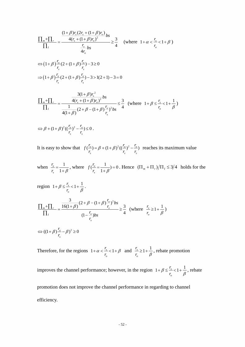
- 52 -
2
(1 ) (2 (1 ) )4( (1 ) ) 3
44
s s o
m r s o
sI
o
r r r bsr r
r bsr
β ββ
+ + ++ + +
= ≥∏ ∏∏
(where 1 1s
o
rr
α β+ < < + )
( )
( )
1 (2 (1 ) ) 3 0
1 (2 (1 ) ) 3 1(2 1) 3 0
o o
s s
o o
s s
r rr rr rr r
β β
β β
⇔ + + + − ≥
⇒ + + + − > + − =
2
2
2
3(1 )4( (1 ) ) 3
1 4(2 (1 ) )4(1 )
s
m r s o
oI
s
r bsr r
r bsr
ββ
β ββ
++ + +
= ≤+ − +
+
∏ ∏∏
(where 11 1s
o
rr
ββ
+ ≤ < + )
2 2(1 ) (( ) ) 0o o
s s
r rr r
β β⇔ + + − ≤ .
It is easy to show that 2 2( ) (1 ) (( ) )o o o
s s s
r r rfr r r
β β= + + − reaches its maximum value
when 11
o
s
rr β=
+, where 1( ) 0
1o
s
rfr β= =
+. Hence ( ) 3 4m r IΠ +Π Π ≤ holds for the
region 11 1s
o
rr
ββ
+ ≤ < + .
23 (2 (1 ) )16(1 ) 3
4(1 )
o
m r s
oI
s
r bsr
r bsr
β ββ
+ − ++ +
= ≥−
∏ ∏∏
(where 11s
o
rr β≥ + )
2((1 ) ) 0o
s
rr
β β⇔ + − ≥
Therefore, for the regions 1 1s
o
rr
α β+ < < + and 11s
o
rr β≥ + , rebate promotion
improves the channel performance; however, in the region 11 1s
o
rr
ββ
+ ≤ < + , rebate
promotion does not improve the channel performance in regarding to channel
efficiency.

- 53 -
3.8. Numerical Studies
This section uses numerical studies to further analyze the impact of the slippage
phenomenon and loss aversion effect on the manufacturer’s profit. Proposition 3.3
provides evidence that the manufacturer’s optimal profit increases with the slippage
rate under rebate promotion. However, it does not quantify the magnitude of the
benefit. Consider an example with the following parameter settings: bs=$300 ,
0.2α = , 0.4β = , 0.9sr = and 0.1 o sr r≤ ≤ at an incremental rate of 0.01. The values
of mΠ , D , R , sP , rP and w are plotted in figure 3.7. From these graphs, we can
observe that the manufacturer’s profits and the market demand increases smoothly
with the slippage rate; however, the curve of the optimal rebate value R increases in
a stepwise fashion with the slippage rate. From graph d, we can observe that the retail
price almost follows the same pattern as the wholesale price, as expected.
[Insert Figure 3.7. here]
Next, I explore how the slippage and loss aversion jointly affect the manufacturer’s
profit. By setting β to be flexible from [ ],0.8α , we can observe from the
three-dimensional graph of Figure 3.8 that the stronger the magnitude of loss aversion,
the larger the manufacturer’s profits. However, the contribution of loss aversion
effects to profits is much smaller than the one brought by slippage effects.
Furthermore, the distinct section line on the graph is the section point where the
manufacturer changes from offering a small-ticketed rebate to a larger one. With
larger magnitude of loss aversion, it is easier for the manufacturer to induce the

- 54 -
retailer to choose the MSRP. In this situation, the manufacturer has higher profit level
with a small-ticket rebate, so a larger slippage rate is required for the manufacturer to
desire to offer a large-ticketed rebate.
[Insert Figure 3.8. here]
3.9. Conclusions
In this chapter, I analyze the impact of rebates and MSRP on a vertical channel with
reference-dependent consumers. Coupled with a rebate promotion, the manufacturer
announces a suggested retail price serving as a reference point for consumers. I find
that the slippage effect and the loss aversion effect jointly impact the manufacturer’s
profit. For the decentralized channel, if the consumers are sufficiently loss averse, i.e.,
21αβα
≥−
, the manufacturer should offer rebates as long as some purchasers end up
forgoing the rebates. On the other hand, if the consumers are not sufficiently loss
averse, the manufacturer chooses to provide rebates only after the slippage rate breaks
a threshold level ( , )θ α β . Under rebate promotions, both the manufacturer’s and the
retailer’s profits increase with the slippage rate and the magnitude of loss aversion.
For the loss-neutral case and the integrated channel, the breakeven slippage rate to
make rebate promotion profitable increases to 1 α+ . According to industry reports,
the slippage rate is ranging from approximately a low rate for 1.7 on electronics
(Spencer 2005) to a very high rate for more than 10 in some categories, such as
software products (Bulkeley 1998). This reveals why so many companies are issuing

- 55 -
rebates nowadays.
Even for a promoted product facing high redemptions, the companies can increase the
slippage rate by adopting appropriate marketing techniques. Rather than increasing
the required redemption effort, previous empirical research has provided several
effective ways in which the manufacturer can exacerbate the consumers’ slippage
behavior. Moorthy and Soman (2003) suggests that properly marketing the rebate can
exacerbate the slippage by highlighting the reward and not highlighting the effort
required to redeem. Silk (2004) suggests that encouraging procrastination and
prospective forgetting also have a great impact on slippage by increasing the length of
the redemption deadline.
Hopefully, the results in this chapter will provide insights for researchers who would
like to further analyze the slippage phenomenon on rebates. One extension would be
to associate the objective probability of redeeming or to the consumer’s type t, i.e.
assuming or is decreasing with t. With this assumption, rebate promotions can
price-discriminate between consumer types after purchase, which implies that high
consumer types have low probability to redeem because they usually have high
redemption costs and low marginal utility of income. Hence, the manufacturer can
possibly achieve higher profits by only serving the high consumer types. Another line
of extension would be to apply this model to the research on new product design. In
that case, the manufacturer can adjust the product quality level s , which has an

- 56 -
increasing cost ( )v s such that the manufacturer needs to determine an optimal
quality level. Since advertising is one important element of the promotional mix,
researchers can also add the advertising cost to initiate the penetration rate.

- 57 -
Figure 3.1. An MSRP Example
Figure 3.2. A Schematic Framework of the Market Environment

- 58 -
Figure 3.3. The Kinked Demand Curve ( , )rD P R

- 59 -
Figure 3.4. A Schematic Framework of Reference-dependent Model
Figure 3.5. A Schematic Framework of Loss-neutral Model
Figure 3.6. A Schematic Framework of Integrated Channel

- 60 -
(a) m∏ versus s or r
(b) D versus s or r
(c) R versus s or r
(d) sP , rP and w versus s or r
Figure 3.7. A Numerical Example
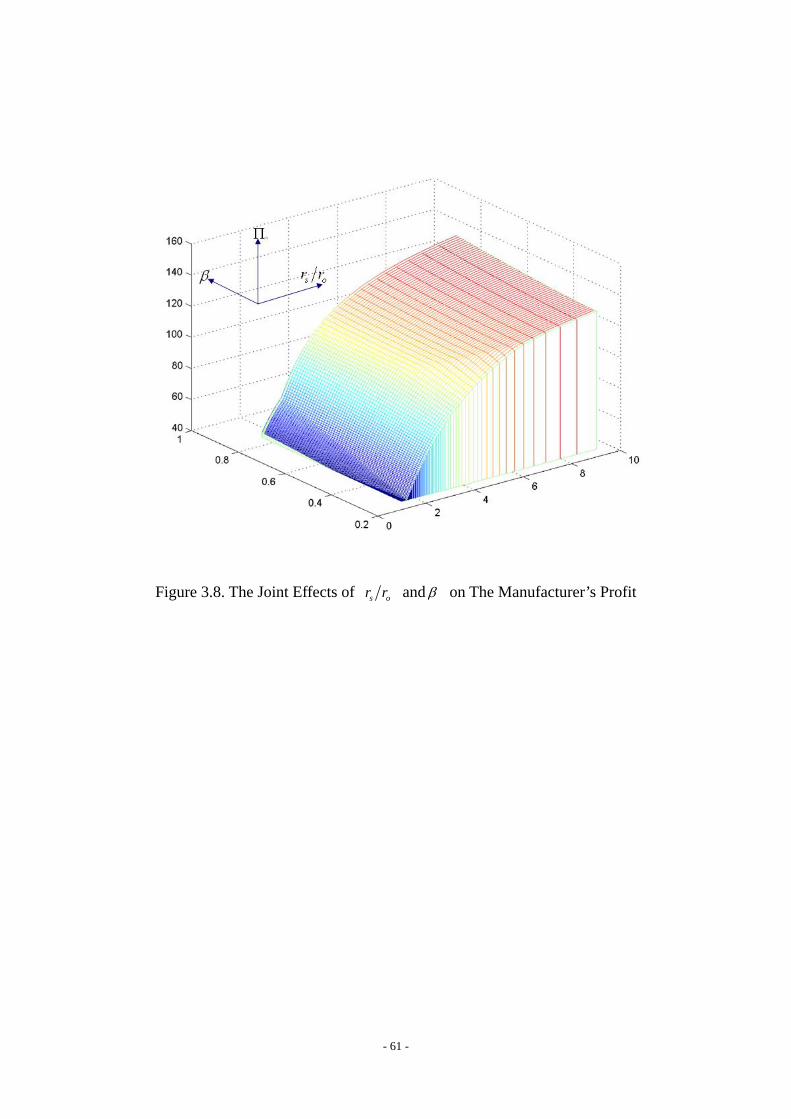
- 61 -
Figure 3.8. The Joint Effects of s or r and β on The Manufacturer’s Profit

- 62 -
ow r R− r oP r R− D rΠ mΠ r mΠ +Π
2bs 3
4bs 1
4
16bs
8bs 3
16bs
Table 3.1. The Equilibrium Solution of Rebate Promotion Only without Slippage
w rP R D rΠ mΠ r mΠ +Π
∞ ∞ ∞ 1 bs ∞ ∞
Table 3.2. The Equilibrium Solution of Rebate Promotion Only with Slippage

- 63 -
NRLS NRES SRES MRHS LRHS b1 c1 c2 d1 d2
Con
ditio
n 1 ( , )s
o
rr
θ α β≤ < 1s
o
rr= ( , ) 1s
o
rr
θ α β β≤ < + 11 1s
o
rr
ββ
+ ≤ < + 11s
o
rr β≥ +
w
2bs
2bs
2(1 )2( (1 ) )
s o
s o
r r bsr r
ββ
+ ++ +
bs 2( )
2 2 2o
s
r bsr
ββ
++
+
R 0 0 12( (1 ) )s o
bsr r
ββ
++ +
(1 )
(1 )s o
bsr r
ββ
++ +
s
bsr
sP bs (3 )
4 2bsββ
++
bs bs bs
rP 34
bs (3 )
4 2bsββ
++
bs 3 2(1 )2( (1 ) )
s o
s o
r r bsr r
ββ
+ ++ +
3(2 )( )4(1 ) 4
o
s
r bsr
ββ
++
+
D 14α+
14 2
ββ
++
(1 )2( (1 ) )
s
s o
rr r
ββ
++ +
(1 )
2( (1 ) )s
s o
rr r
ββ
++ +
1 (2 (1 ) )4
o
s
rr
β β+ − + ⋅
rΠ 116
bsα+
2
14(2 )
bsββ
++
2
2
(1 )4( (1 ) )
s
s o
r bsr r
ββ
++ +
2
2
(1 )4( (1 ) )
s
s o
r bsr r
ββ
++ +
21 (2 (1 ) )
16(1 )o
s
r bsr
β ββ
+ − ++
mΠ 18
bsα+ 1
4(2 )bsβ
β++
(1 )
4( (1 ) )s
s o
r bsr r
ββ
++ +
2
2
(1 )2( (1 ) )
s
s o
r bsr r
ββ
++ +
21 (2 (1 ) )8(1 )
o
s
r bsr
β ββ
+ − ++
r mΠ +Π 3(1 )16
bsα+ 2
(1 )(3 )4(2 )
bsβ ββ
+ ++
2
(1 ) (2 (1 ) )4( (1 ) )
s s o
s o
r r r bsr r
β ββ
+ + ++ +
2
2
3(1 )4( (1 ) )
s
s o
r bsr r
ββ
++ +
23 (2 (1 ) )
16(1 )o
s
r bsr
β ββ
+ − ++
Table 3.3. The Equilibrium Solution Sets of Reference-dependent Model3
3 At the corner points, i.e., when 1s or r = with 2 (1 )β α α= − , ( , )s or r θ α β= and 1s or r β= + , the equilibrium solution can be any combination of the two consecutive solution sets. For example, when
1s or r β= + , * 2(1 ) (1 )2( (1 ) )
s o
s o
r rw bs bsr r
βκ κ
β+ +
= ⋅ + − ⋅+ +
, where [ ]0,1κ ∈ is a fraction parameter.

- 64 -
NRLS MSHS LRHS Condition
1s
o
rr
α≤ + 11 1s
o
rr
αα
+ < < + 11s
o
rr α≥ +
w
2bs
bs 2( )
2 2 2o
s
r bsr
αα
++
+
R 0 (1 )(1 )s o
bsr r
αα
++ +
s
bsr
sP bs bs bs
rP 34
bs 3 2(1 )2( (1 ) )
s o
s o
r r bsr r
αα
+ ++ +
3(2 )( )4(1 ) 4
o
s
r bsr
αα
++
+
D 14α+
(1 )2( (1 ) )
s
s o
rr r
αα
++ +
1 (2 (1 ) )4
o
s
rr
α α+ − + ⋅
rΠ 116
bsα+ 2
2
(1 )4( (1 ) )
s
s o
r bsr r
αα
++ +
21 ((2 (1 ) )16(1 )
o
s
r bsr
α αα
+ − ++
mΠ 18
bsα+ 2
2
(1 )2( (1 ) )
s
s o
r bsr r
αα
+⋅
+ +21 ((2 (1 ) )
8(1 )o
s
r bsr
α αα
+ − ++
r mΠ +Π 3(1 )16
bsα+ 2
2
3(1 )4( (1 ) )
s
s o
r bsr r
αα
++ +
23 ((2 (1 ) )16(1 )
o
s
r bsr
α αα
+ − ++
Table 3.4. The Equilibrium Solution Sets of Loss-neutral Model.4
4 At the corner point where 1s or r α= + , the equilibrium solution can be any combination of the two consecutive solution sets NRLS and MSHS.

- 65 -
NRLS SMRES LRHS LRES b1 c2-1 d a2
Con
diti
on 1s
o
rr
α≤ + 1 1s
o
rr
α β+ < < +11 1s
o
rr
ββ
+ ≤ < + 11s
o
rr β≥ +
R 0
2 o
bsr
s
bsr
s
bsr
sP bs bs bs bs
rP 2bs
bs 2( )
2 2 2o
s
r bsr
ββ
++
+
bs
D 12α+
2
s
o
rr
1 (2 (1 ) )2
o
s
rr
β β+ − + 1
IΠ (1 )4
bsα+
4s
o
r bsr
21 (2 (1 ) )4(1 )
o
s
r bsr
β ββ
+ − ++
(1 )o
s
r bsr
−
Table 3.5. The Equilibrium Solution Sets of Integrated Channel5
5 At the corner points, i.e., when 1s or r α= + and 1s or r β= + , the equilibrium solution can be any combination of the two consecutive solution sets

- 66 -
CHAPTER 4
COORDINATING CONTRACTS UNDER SALES PROMOTION

- 67 -
4.1. Brief Introduction
In a decentralized supply chain, channel members acting independently usually
cannot achieve optimal performance of the supply chain due to the double
marginalization problem (Spengler 1950). To improve supply chain performance, the
coordination mechanism between upstream manufacturers and downstream retailers
has been studied extensively in recent years. A contract is widely used between
independent channel members to prevent a unilateral deviation from the set of
globally optimal actions. This chapter examines contracting coordination issues under
sales promotion in a supply chain. I build a three-way promotion loop in a supply
chain by including all three types of sales promotions (consumer promotions, retailer
promotions, and the trade dealings). Because sales promotion is indispensable in
business, such three-way promotions frequently occur in practice. When the
manufacturer launches a consumer promotion (such as rebates or coupons), the
retailer usually performs multiple follow-up promotional tasks (such as in-store
displays, feature advertising, etc) to leverage the manufacturer’s consumer promotion
and spur even more market demand.
Among various techniques of consumer promotions, mail-in rebates offered by the
manufacturer can bypass the retailer and reach consumers directly. Usually the
consumers are eligible to redeem the rebates as long as they purchase the required
products. However, there has been a tendency in recent years to apply rebate
promotions only to a limited set of retailers or even a single cooperative retailer. The

- 68 -
following rebate promotion is provided by Logitech and requires purchasing from
Amazon.com only.
[Insert Figure 4.1. here]
Apparently, there are some cooperative promotions uniquely existing between these
two supply chain partners. So a properly designed contract can certainly improve the
performance of the sales promotion.
We consider the following two-echelon system in a single selling season
(newsvendor-like) environment. The manufacturer chooses the rebate face value and
the wholesale price, where both are observable and verifiable (i.e., contract
instruments). Facing the manufacturer’s rebate promotion, the retailer acting as a
newsvendor chooses order quantity and promotional effort level before the selling
season starts. However, due to the moral hazard problem (see p.27 on literature
review for reference), the retailer’s promotional effort cannot be written into contract,
hence, cost sharing is not possible in contracting. As shown in previous literature,
traditional contracts (i.e., wholesale, buy-back, revenue sharing, channel rebates)
offered by the manufacturer are not sufficient to coordinate the supply chain, in part
because these contracts fail to align the retailer’s incentives (i.e., the order quantity
and the promotional effort level). I show that a quantity discount contract with
buy-back is sufficient to coordinate the supply chain with stochastic market demand.

- 69 -
To the best of my knowledge, this is one of the first papers in the coordination
literature that specifically studies the manufacturer’s rebate promotion and the
retailer’s promotional effort simultaneously in a general setting. The rest of the
chapter is organized as follows. Model development (descriptions, assumptions and
notations) are presented in section 4.2. Section 4.3 analyzes the deterministic demand
model which is usually favored by the marketing literature. Section 4.4 analyzes the
stochastic demand model which usually exists in operations literature. Section 4.5
contains the numerical examples. Finally, section 4.6 concludes this chapter. The
flowchart below reveals a layout of the discussed contracts in the rest of the chapter.
[Insert Figure 4.2. here]
4.2. Model Development
This section describes the basic model setting. Given the short life cycle of many
products (such as software and electronics) and the short-term nature of promotions, a
one-period model is employed. This approach is consistent with the contracting
literature where one-period models are widely used. This model may also serve as an
approximation for time-restricted promotions for longer life-cycle products. In this
model, the manufacturer can only sell products to final consumers through the retailer,
i.e., no direct sales can occur.
- 70 -
The retail price is exogenously given by the market, i.e. the retailer cannot dictate the
pricing. The exogenous retail price has been used previously in contracting literature
(Taylor 2001, Krishnan et al. 2004, Netessine and Rudi 2000). This assumption can be
justified under a sufficiently competitive market where retailers are price takers.
Alternatively, in the durable goods market, manufacturers may have control over the
retail price by employing manufacturer suggested retail price (MSRP) or resale price
maintenance (see Gurnani and Xu 2006 for explicit resale price maintenance
discussion).
As two different types of sales promotion, rebate promotion and retailer promotional
effort (see p.27 on literature review for reference) should have dissimilar effects on
consumer demand. I assume that the rebate influences consumer demand in an
additive fashion; however, the retailer’s effort could influence demand in a
multiplicative way, i.e.,
( , ) ( )sD R e ar R eξ= +
where
a is a scaling coefficient for the impact of the rebate promotion
sr is the consumers’ subjective redemption confidence at the time of purchase
R is the rebate face value, a decision variable of the manufacturer
e is the level of promotional effort, a decision variable of the retailer.
ξ is the demand given by a random variable with density ( )f ξ and distribution

- 71 -
( )F ξ .
This functional form of demand can be justified from the existing marketing literature
(Neslin 2002), as retailer efforts (features and displays) have been shown to add
significantly to the effectiveness of temporary price reduction. Even if there is no
accompanying price discount, features and displays can increase sales dramatically
(Inman et al. 1990). I believe effects of rebates on sales are similar to the effects of
price discount, but in a delayed manner to the consumer. So the retailer’s promotional
effort is assume to be stochastically related to the demand, however effect of rebate
promotion is deterministically related to the demand.
The manufacturer serves as the Stackelberg leader and the retailer serves as the
follower. The manufacturer first sets a linear wholesale price w , announces the rebate
face value R , and may offer the retailer a conditional ex post transfer payment
T (such as channel rebate, buy-back credit, markdown allowance). Given the
manufacturer’s decisions, the retailer then places an order with the manufacturer and
chooses the effort level before observing the state of underlying demand ξ . With
symmetric information, the manufacturer and the retailer are risk neural, and both
seek to maximize their own profits. Neither the manufacturer nor the retailer incurs
any goodwill penalty cost if inventories are insufficient to meet market demand, and I
also assume the product has no salvage value.
Given the value of w and R from manufacturer, the retailer’s profit function is

- 72 -
given as
( )( , ) min ,( ) ( )r sQ e w Q p E Q ar R e V e Tξ= − ⋅ + ⋅ ⎡ + ⎤ − +⎣ ⎦∏ ,
where
Q is the order quantity, a decision variable of the retailer
w is the wholesale price, a decision variable of the manufacturer
p is the exogenous retail price
T is the conditional ex post transfer from the manufacturer to the retailer
( )V e is the retailer’s cost of exerting e level of effort, which is convex, increasing,
and continuously differentiable in e for any 0e ≥ , with ( )0 0V = .
Anticipating the retailer’s proper profit maximizing reaction ( )* *,Q e , the
manufacturer’s profit function can be written as
( )* * *( , ) ( ) ( , ) min ( , ), ( ) ( , )m o sw R w c Q w R r R E Q w R ar R e w R Tξ⎡ ⎤= − ⋅ − ⋅ + −⎣ ⎦∏ ,
where
c is the manufacturer’s unit production cost
or is consumers’ objective probability of redeeming the rebate after the purchase.
The logical boundary conditions are listed below:
(A1) 0 c w p< < < ,
(A2) 0R ≥ , ow c r R> + , 0e ≥ ,
(A3) 0 1o sr r< ≤ ≤ ,
(A4) ( ) 0f ξ > for all 0ξ > .
- 73 -
4.3. The Deterministic Demand Model
When the market demand is certain, the retailer’s order quantity Q is equivalent to the
market demand D. So the original problem reduces to a pricing and promotion
problem to find the optimal demand. I use ( )u E ξ= represent a constant basic
demand. The retailer’s and the manufacturer’s profit functions become
( )( ) ( )r sp w ar R u e V e= − + −∏ ,
( )( )m o sw c r R ar R u e= − − +∏ ,
respectively. For an integrated channel, the profit function follows as
( , ) ( ) ( , ) ( ) ( )( R ) ( )I o o sR e p c r R D R e V e p c r R ar u e V e= − − − = − − + −∏ .
Since ( )V e is convex in e and ( , )D R e is linear in R and e , ( , )I R e∏ is strictly
concave in both R and e . The above profit function is assumed to be well behaved
such that a unique maximizing solution * *( , )R e exists with finite arguments, i.e., the
Hessian matrix of ( , )I R e∏ is negative definite. For all ow c r R> + , r I
e e∂ ∂
<∂ ∂∏ ∏ .
So the retailer always exerts a lower than optimal promotional effort; hence, a simple
wholesale price contract cannot coordinate the supply chain unless the retailer keeps
all realized profit. It is easy to show that a contract of sharing rebate cost or sharing
revenue does not coordinate either.
4.3.1. Quantity Discount Contract
Consider a quantity discount contract where the manufacturer offers the retailer a
varying wholesale price according to the quantity ordered by the retailer. The larger
the quantity ordered, the lower the wholesale price. From the demand function,
- 74 -
( )sD ar R u e= + , there is a one-to-one relationship between e and D for any given
value of R by the manufacturer. So the retailer’s promotional effort level can be
represented by a function of market demand and rebate face value, i.e.,
( , )s
De D Rar R u
=+
. For integrated channel, the profit function can be written as
[ ]( , ) ( ) ( , )I oD R p c r R D V e D R= − − −∏ .
Theorem 4.1. There exists an all-units quantity discount contract ( , )w D R that
coordinates the supply chain.
(a)The quantity discount schedule is given by
[ ]21 1 1
( , )( , ) (1 )( )o
V e D Rkw D R k p k c r R kD D
= + − + + − ,
where ( )1 0,1k ∈ and 2k are profit-splitting parameters between the manufacturer
and the retailer.
(b) The resulting profits to the manufacturer and the retailer are
* *1 2( , )m Ik D R k= +∏ ∏ and * *
1 2(1 ) ( , )r Ik D R k= − −∏ ∏ , respectively.
Under this specification, the wholesale price is jointly determined by the market
demand and the rebate value. Furthermore, as long as the demand elasticity of
[ ]( , )V e D R , i.e., /
V DV D∂ ∂ , is greater than one, ( )w D is indeed a quantity discount
schedule for any 2 0k ≥ . This property is intuitive: as the order quantity increase, the
promotional cost increases by a larger percentage. The property 1/
V DV D∂ ∂
> holds for
most realistic promotional effort cost function. For example, assume 2( ) 2V e be=
(see Taylor, 2002), where 0b > can be interpreted as the costliness of effort, we have

- 75 -
2 1/
V DV D∂ ∂
= > .
With this quantity discount contract, the retailer’s profit function becomes
[ ] [ ]{ }1 2( ) ( ( , )) ( , ) (1 ) ( ) ( , )r oD p w D R D V e D R k p c r R D V e D R k= − − = − − − − −∏ .
The retailer now faces the same decision problem as the one in integrated channel.
Thus, the profit maximizing behavior of the retailer is consistent with the channel
profit maximizing behavior, implying that the retailer will choose the
channel-optimizing order quantity as well as the cannel-optimizing level of
promotional effort. The manufacturer’s profit is also linearly related to the channel
profit, implying that the manufacturer will choose the channel-optimizing rebate face
value contingent that *D is chosen by the retailer. Therefore, this quantity discount
scheme ( , )w D R can coordinate the supply chain by inducing the retailer to order
more and resulting in exerting the optimal promotional effort. The intuition behind
this is that the discount scheme has been designed so that the retailer’s marginal cost
is equal to its marginal revenue p at the point *D ,, i.e.,
( ) [ ]1 1
( , )( , ) ( , ) (1 )( )o
V e D Rw D R D V D R k p k c r R
D D∂∂
+ = + − + +∂ ∂
, where
[ ] *( , ) oD DV e D R D p c r R
=∂ ∂ = − − . The discount scheme indicates that supply chain
coordination involves a sharing of rebate cost, i.e., the retailer needs to share
1100(1 )%k− of each redeemed rebate.
The quantity discount schedule in Theorem 4.1 is a continuous one. A coordinating
discrete discount schedule can also be developed. Previous theoretic results (Weng

- 76 -
1995) already predict that one price break at *D is sufficiently enough to coordinate
the supply chain under a deterministic model. With the assumption that a discrete
discount policy would appeal to the retailer only if its profit will increase by no
smaller than (1 ) 100%λ+ × , the following corollary explains the coordinating
mechanism with a discrete schedule.
Theorem 4.2. There exists a discrete quantity discount contract that coordinates the
supply chain.
(a) The quantity discount schedule is given by { }1 1 2 2( , ), ( , )w R w R with price break at
*D such that
( )( )*2 2 1 1 2 1 1 1 1 2*
1( , , ) (1 ) ( ) [ ( , )] [ ( , )]w w w R R p p w D V e D R V e D RD
λ= = − + − − + , where 1D is
the solution of the equation 1
11
[ ( , )]
D D
V e D R p wD =
∂= −
∂.
(b) The resulting profits to the manufacturer and retailer are
( )* *1 1 1 1( , ) (1 ) ( ) [ ( , )]d
m I D R p w D V e D RλΠ =Π − + − − and
1 1 1 1(1 )(( ) [ ( , )])dr p w D V e D RλΠ = + − − , respectively.
The legality issue of proposed quantity discount contracts can be justified by arguing
a cost savings by producing for a large order size (Jeuland and Shugan 1983). Hence,
as long as the promotional cost structures of different retailers are similar, then
retailers will not pay different prices for the same order quantities. Thus, my proposed
contracts are legal under Robinson Patman Act, which prohibits offering different
terms to different retailers in the same retailer class. However, if the retailers have

- 77 -
significantly different promotional cost structures, the proposed discount schemes
may not be directly applicable because different retailer will end up paying a different
unit wholesale price.
4.3.2. Two-part Tariff Contract
In practice, quantity discount are often implemented as a set of two-part tariff contract,
especially in the extent of franchised chains. A typical set of two-part tariff contract
involves a fixed payment and per-unit charges, i.e. the retailer pays an initial fee F
for buying any amount of the product plus a constant wholesale price w . The
following two-part tariff contract achieves cannel coordination,
* *1 2( ) ( ) ( , ) ( )oF R k p c r R D e R V e k⎡ ⎤= − − − +⎣ ⎦ ,
( ) ow R c r R= +
where ( )1 0,1k ∈ and 2k are profit-splitting parameters,
*e is the optimal promotional effort in the integrated channel.
The cost of the rebate has been shared in the fixed initial fee by the retailer. The main
idea behind this contract is that the retailer keeps all realized revenues such that it will
exert the correct amount of promotional effort. The retailer’s profit function is
* *1 2
( ( )) ( , ) ( ) ( )
( ) ( , ) ( ) ( ) ( , ) ( ) .r
o o
p w R D e R V e F R
p c r R D e R V e k p c r R D e R V e k
Π = − − −
⎡ ⎤= − − − − − − − −⎣ ⎦
Since the above function is linearly related to the integrated channel profits, the
retailer’s profit maximizing is equivalent to the channel’s maximizing problem. Hence,
the retailer will choose the channel optimal promotional effort level. For the

- 78 -
manufacturer,
* *1 2( ) ( , ) ( ) ( , ) ( )m o ow c r R D e R F k p c r R D e R V e k⎡ ⎤Π = − − + = − − − +⎣ ⎦ .
So as long as the retailer chooses the optimal decisions ( i.e., *e ), the manufacturer’s
profit is also maximized. So the supply chain achieves coordination, and the split of
profits between the manufacturer and the retailer is exactly the same as the quantity
discount contract.
The proposed continuous quantity discount contract and the two-part tariff contract
also function properly in situations where the retailer (like Wal-Mart) has more
bargaining power, and acts as a leader by offering a contract to the manufacturer. The
same quantity discount scheme still coordinate the supply chain, and the two-part
tariff contract can also work after adjusting the fixed fee to
*1 2( ) ( ) ( , ) ( )oF e k p c r R D e R V e k⎡ ⎤= − − − +⎣ ⎦ .
4.4. The Stochastic Demand Model
When the market demand is stochastic, we have the following demand function
( , ) ( )sD R e ar R eξ= + .
Let the density function and distribution function of ( , )D R e be ( | , )y R eφ and
( | , )y R eΦ , respectively. From the distribution of ξ , it is straightforward to show that
1( | , ) ( )syy R e f ar R
e eφ = − , and
R
1( | , ) ( ) ( )s
ys sar e
y yy R e f ar R dy F ar Re e e
Φ = − = −∫ .

- 79 -
As a benchmark, suppose that the manufacturer owns the retailer, i.e., the case of
integrated channel. For the integrated channel, the manufacturer faces a newsvendor
problem with three decision actions: the production quantity Q , the level of
promotional effort e, and the rebate face value R. Let ( , , )S Q R e be expected sales,
( )min ,E Q D⎡ ⎤⎣ ⎦ ,
( )
0
( , , ) min ,(
(1 ( | , )) ( | , )
( | , )
( )
( ) .
s
s
s
s
s
Q
ar eR
Q
ar eR
Qsar eR
Q ar Re
S Q R e E Q ar R e
Q Q R e y y R e dy
Q y R e dy
yQ F ar R dye
Q e F y dy
ξ
φ
−
= ⎡ + ⎤⎣ ⎦
= −Φ +
= − Φ
= − −
= −
∫
∫
∫
∫
4.4.1. Centralized Supply Chain
As a benchmark, suppose the manufacturer owns the retailer. The profit function of
the integrated channel is
( )
0
( , , ) ( ) min ,( ( )
( ) ( ) ( ) ( ).s
I o s
Q ar Re
o o
Q R e cQ p r R E Q ar R e V e
p r R c Q p r R e F y dy V e
ξ
−
= − + − ⋅ ⎡ + ⎤ −⎣ ⎦
= − − − − −
∏
∫
Lemma 4.1. ( , , )I Q R eΠ is strictly concave in Q , R and e .
Proof: See Appendix
We assume that the function ( )V e and the demand distribution are chosen such that
the channel profit function IΠ is well-behaved, i.e., the existence of an optimal
solution ( , , )I I IQ R e is assured in the feasible area (i.e., satisfying all assumptions
A1-A4). The optimal solution should satisfy the following first-order conditions:

- 80 -
( )I I I IsQ ar R Q e= + (4.1)
0( )QI I
II
o s
Q e F y dyp cRr ar e
−−= − ∫
(4.2)
0( ) | ( ) ( ) ( )
I
I
IQI I
o Ie e
QV e p r R F Q F y dye e=
⎛ ⎞∂= − ⋅ −⎜ ⎟∂ ⎝ ⎠
∫ (4.3)
where 1( )I
I oI
o
p r R cQ Fp r R
− − −=
−.
By embedding (4.1) into (4.2) and (4.3), we can get
0( )
2 2
IQII
o s
Q F y dyp cRr ar
−−= − ∫
(4.4)
( )0
0
( ) | ( ) ( ) ( ) ( )
( ) ( ) ( )
I
I
I
QI I I Io se e
QI I Is o o
V e p r R ar R Q F Q F y dye
ar p r R c R p r R ydF y
=
∂= − + −
∂
= − − + −
∫
∫ (4.5)
So IR can be obtained by solving (4.4) 1. Note that the optimal rebate value is not
related to the cost structure of ( )V e . With IR , we can get Ie and IQ sequentially
from (4.5) and (4.1). Let IΠ denote the corresponding maximum profits for the
integrated channel.
0( , , ) ( ) ( ) ( ) ( )
( ) ( ) | ( ) ( ) ( )
( ) | ( ).
I Is
I
I
I
Q ar RI I I I I I I Ie
I o o
I I I I I I Io oe e
I Ie e
Q R e p r R c Q p r R e F y dy V e
p r R c Q e V e p r R Q F Q V ee
e V e V ee
−
=
=
Π = − − − − −
∂= − − + − − −
∂∂
= −∂
∫
The above profit function is in the same form as the one in Taylor (2002), which does
not include rebate promotions.
1 Multiple complex solutions of equation 4.4 exist, depending on the demand distribution. For example, if the basic demand is uniformly distributed, equation 4.4 is a cubic function, which has at least one real number root. For most of the realistic parameter settings, equation 4.4 has only one solution falling in the feasible area. In particular, if a feasible solution does not exist, the optimal value of the rebate is zero.
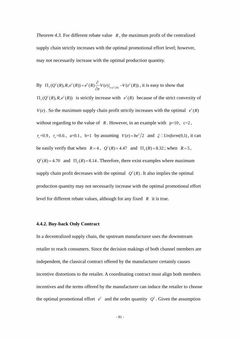
- 81 -
Theorem 4.3. For different rebate value R , the maximum profit of the centralized
supply chain strictly increases with the optimal promotional effort level; however,
may not necessarily increase with the optimal production quantity.
By ( )
( ( ), , ( )) ( ) ( ) | ( ( ))II I I I
I e e RQ R R e R e R V e V e R
e =
∂Π = −
∂, it is easy to show that
( ( ), , ( ))I II Q R R e RΠ is strictly increase with ( )Ie R because of the strict convexity of
( )V e . So the maximum supply chain profit strictly increases with the optimal ( )Ie R
without regarding to the value of R . However, in an example with p=10 , c=2 ,
=0.9sr , =0.6or , a=0.1 , b=1 by assuming 2( ) 2V e be= and (0,1)Uniformξ , it can
be easily verify that when 4R = , ( ) 4.47IQ R = and ( ) 8.32I RΠ = ; when 5R = ,
( ) 4.70IQ R = and ( ) 8.14I RΠ = . Therefore, there exist examples where maximum
supply chain profit decreases with the optimal ( )IQ R . It also implies the optimal
production quantity may not necessarily increase with the optimal promotional effort
level for different rebate values, although for any fixed R it is true.
4.4.2. Buy-back Only Contract
In a decentralized supply chain, the upstream manufacturer uses the downstream
retailer to reach consumers. Since the decision makings of both channel members are
independent, the classical contract offered by the manufacturer certainly causes
incentive distortions to the retailer. A coordinating contract must align both members
incentives and the terms offered by the manufacturer can induce the retailer to choose
the optimal promotional effort Ie and the order quantity IQ . Given the assumption

- 82 -
that the retailer’s promotional level is not contractible, a possible solution can only
contract on order quantity or market sales.
Under a wholesale price contract, the retailer’s profit function is
0( , ) ( , , ) ( ) ( ) ( ) ( )s
Q ar Rw er Q e wQ p S Q R e V e p w Q pe F y dy V e−= − + ⋅ − = − − −∏ ∫ .
For any given order quantity Q and rebate value R , the following first-order
condition of promotional effort is necessary for coordination (but not sufficient),
0
( , ) ( ) ( ) ( ) 0sw Q ar Rr e
sQ e Q Qp F ar R F y dy V e
e e e e−∂ ∂⎛ ⎞= ⋅ − − − =⎜ ⎟∂ ∂⎝ ⎠
∏∫ .
However it is greater than ( , , )I Q e R e∂ ∂∏ for any positive rebate value. As a result,
the retailer exerts a higher than optimal effort. Therefore a wholesale price contract
does not coordinate the supply chain.
Next, consider a buy-back contract where the manufacturer charges the retailer a
wholesale price w but pays the retailer credit b per unit remaining at the end of the
season. The retailer’s profit function is
( )
0
( , ) ( , , ) ( , , ) ( )
( ) ( ) ( ) ( ).s
br
Q ar Re
Q e wQ p S Q R e b Q S Q R e V e
p w Q p b e F y dy V e−
= − + ⋅ + − −
= − − − −
∏
∫
For any given order quantity Q and rebate value R , the retailer chooses the
following promotional effort to maximize its profit,
0
( , ) ( ) ( ) ( ) ( ) 0sb Q ar Rr e
sQ e Q Qp b F ar R F y dy V e
e e e e−∂ ∂⎛ ⎞= − ⋅ − − − =⎜ ⎟∂ ∂⎝ ⎠
∏∫ .
Compared to the channel profit function, i.e.,
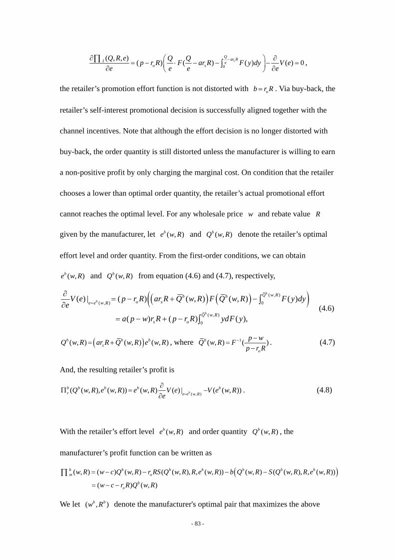
- 83 -
0
( , , ) ( ) ( ) ( ) ( ) 0sQ ar RI e
o sQ R e Q Qp r R F ar R F y dy V ee e e e
−∂ ∂⎛ ⎞= − ⋅ − − − =⎜ ⎟∂ ∂⎝ ⎠∏
∫ ,
the retailer’s promotion effort function is not distorted with ob r R= . Via buy-back, the
retailer’s self-interest promotional decision is successfully aligned together with the
channel incentives. Note that although the effort decision is no longer distorted with
buy-back, the order quantity is still distorted unless the manufacturer is willing to earn
a non-positive profit by only charging the marginal cost. On condition that the retailer
chooses a lower than optimal order quantity, the retailer’s actual promotional effort
cannot reaches the optimal level. For any wholesale price w and rebate value R
given by the manufacturer, let ( , )be w R and ( , )bQ w R denote the retailer’s optimal
effort level and order quantity. From the first-order conditions, we can obtain
( , )be w R and ( , )bQ w R from equation (4.6) and (4.7), respectively,
( ) ( )( )( , )
( , ) 0
( , )
0
( ) | ( ) ( , ) ( , ) ( )
( ) ( ) ( ),
b
b
b
Q w Rb bo se e w R
Q w Rs o
V e p r R ar R Q w R F Q w R F y dye
a p w r R p r R ydF y
=
∂= − + −
∂
= − + −
∫
∫ (4.6)
( )( , ) ( , ) ( , )b b bsQ w R ar R Q w R e w R= + , where 1( , ) ( )b
o
p wQ w R Fp r R
− −=
−. (4.7)
And, the resulting retailer’s profit is
( , )( ( , ), ( , )) ( , ) ( ) | ( ( , ))b
b b b b br e e w R
Q w R e w R e w R V e V e w Re =
∂Π = −
∂. (4.8)
With the retailer’s effort level ( , )be w R and order quantity ( , )bQ w R , the
manufacturer’s profit function can be written as
( )( , ) ( ) ( , ) ( ( , ), , ( , )) ( , ) ( ( , ), , ( , ))
( ) ( , )
b b b b b b bm o
bo
w R w c Q w R r RS Q w R R e w R b Q w R S Q w R R e w R
w c r R Q w R
= − − − −
= − −
∏
We let ( , )b bw R denote the manufacturer's optimal pair that maximizes the above

- 84 -
profit function, and bmΠ is the corresponding manufacturer’s maximum profit. With
( , )b bw R chosen by the manufacturer, the retailer’s maximum profit brΠ can be
obtained.
Theorem 4.4. Suppose ( ) kV e be= ( 2k ≥ ), where 0b > can be interpreted as the
costliness of effort. The efficiency of the buy-back contract ( ( )b bm r IΠ +Π Π ) and the
manufacturer’s optimal decisions on ( , )w R is not influenced by the value of b .
Proof: See Appendix
It also can be shown that identical results for the parameter b also hold under a
wholesale price contract.
The following lemma also holds for any given rebate face value.
Lemma 4.2. For any given rebate value R , ( ( ), )b bQ w R R is strictly less than ( )IQ R .
Proof: See Appendix
Lemma 4.2 characterize the optimal quantity decision for any given rebate face value,
which serves as a base for the discrete quantity discount in the following section.
In this section, I show that a buy-back contract by itself is not enough to coordinate a
supply chain. However, a buy-back contract does not distort the retailer’s promotional
decision. Based on this, two coordinating contracts are proposed in the following.
4.4.3. Continuous Quantity Discount Contract with Buy-back

- 85 -
Inspired by Cachon and Lariviere (2005), where the authors find that a continuous
quantity discount contract can coordinate the supply chain with the retailer’s
promotional effort, I propose a continuous quantity discount schedule with buy-back
contract that can coordinate a supply chain.
Theorem 4.5. There exists a continuous all-unit quantity discount contract with
buy-back ( )( , ),w Q R b that coordinates the supply chain.
(a)The quantity discount schedule is given by
21 1
( , , )( , ) ( ) (1 )I
o okS Q R ew Q R k p r R r R k c
Q Q= − + + − +
and the buy-back credit is given by ( ) ob R r R= .
(b) The resulting profits to the manufacturer and the retailer are
1 1 2( , , ) ( )I I I Im Ik Q R e k V e k= + +∏ ∏ and 1 1 2(1 ) ( , , ) ( )I I I I
r Ik Q R e k V e k= − Π − −∏ ,
respectively.
where Ie is the optimal effort level in the integrated channel
( )1 0,1k ∈ and 2k are profit-splitting parameters
Proof: See Appendix.
With this quantity discount contract with buy-back, the retailer keeps all the revenues
such that it will choose the optimal promotional effort as in the integrated channel.
Coordination occurs because the retailer’s effort decision is not distorted, and its order
quantity decision is adjusted contingent that Ie is chosen; subsequently, the
manufacturer’s rebate value decision is adjusted contingent that Ie and IQ are

- 86 -
chosen. Moreover, for a special case, if 2 1 ( )Ik k V e= − , the profit can be shared exactly
between the manufacturer and the retailer with a percentage rate 1k .
4.4.4. Discrete Quantity Discount Contract with Buy-back
The continuous quantity discount contract with buy-back achieves coordination
because the retailer’s expected profit is proportional to the supply chain’s expected
profit under the proposed contract. As long as the promotional cost structures of
different retailers are similar, my proposed contract is legal under Robinson Patman
Act.
However, although continuous discount schedule is popular in academia (See Jeuland
and Shugan 1983, Cachon and Lariviere 2005 for examples), the infinite number of
price breaks associated with continuous discount is definitely not welcomed by the
managers in practice. In a field study by Munson and Rosenblatt (1998), the authors
say “none of the participants have seen continuous schedules in practice”, and they
suggest researchers should especially “shy away from continuous discount schedules”.
So I create a discrete discount schedule with one price break, and then test whether
the manufacturer can design a quantity discount contract with buy-back which can
sufficiently coordinate the supply chain.
In my proposed contract, the manufacturer offers a quantity discount schedule with
only one price breaks at dQ , i.e., the manufacturer offers two pairs of wholesale price

- 87 -
and rebate value as follows: if the retailer’s order quantity Q is less than dQ , the
manufacturer charges a basic wholesale price 1w and announce a rebate promotion
with 1R ; if Q is greater than or equal to dQ , the manufacturer charges a discounted
wholesale price 2w (where 2 1w w< ) and announce a rebate promotion with 2R .
After the selling season ends, the retailer can return the leftovers to the manufacturer
with ob r R= . The objective of the manufacturer is to offer a quantity discount
schedule such that the retailer will always order at the level 2w w= , which is
equivalent to maximizing the manufacturer's profit at 2w w= subject to the constraint
that the retailer’s maximum profit earned at the level 2w w= is no smaller than its
profit earned by ordering at the 1w w= level.
The retailer would be willing to order at a discounted wholesale price 2w only if its
profit would not decreases by ordering dQ Q≥ . The retailer’s profit function can be
given by,
( )2
2 0
( , | ) ( , , ) ( , , ) ( )
( ) ( ) ( ) ( ).s
dr
Q ar Re
o
Q e Q Q w Q pS Q R e b Q S Q R e V e
p w Q p r R e F y dy V e−
Π ≥ = − + + − −
= − − − −∫
Let Q′ be the unconstrained optimal order quantity, i.e.,
( ) 1 22 2 2 2 2 2 2
2
, ( , ), ( ) ( , )so
p wQ w e w R R F ar R e w Rp r R
−⎛ ⎞−′ = +⎜ ⎟−⎝ ⎠. Because the retailer’s profit
function is piecewise concave in order quantity, the retailer will choose either Q′ or
dQ . Directly from Lemma 4.2, we have 2 2 2( , ) ( )IQ w R Q R′ < . Hence, to induce the
retailer to choose the same optimal order quantity IQ in the integrated channel, we
must have IQ as the price breakpoint, i.e. IdQ Q= , such that the retailer’s profit is

- 88 -
maximized at IQ Q= .
I assume that a quantity discount policy would appeal to the retailer only if its profit
will increase by no smaller than (1 ) 100%λ+ × . I propose the following contract.
Theorem 4.6. There exists a discrete quantity discount contract with buy-back that
coordinates the supply chain.
(a) The quantity discount schedule is given by { }1 1 2 2( , ), ( , )w R w R with price break at
IQ such that
22( )
2 2 1 1 2 1 1 2 2 20
1( , , ) (1 ) ( , ) ( ) ( ) ( ) ( ( ))I
sdQ ar R
e Rb d dr oIw w w R R p w R p r R e R F y dy V e R
Qλ
−⎛ ⎞⎜ ⎟= = − + Π + − +⎜ ⎟⎝ ⎠
∫ ,
where 1 1( , )br w RΠ and 2( )de R are obtained from (4.8) and (4.9) in appendix,
respectively.
(b) The buy-back credit is given by ( ) ob R r R= accordingly.
(c) The resulting profits to the manufacturer and retailer are
1 1(1 ) ( , )d bm I r w RλΠ =Π − + Π and 1 1(1 ) ( , )d b
r r w RλΠ = + Π , respectively.
Proof: See Appendix.
Note that under coordination, the arbitrary profit splitting can be achieved by
choosing a sufficiently large 1w (which results in 1 1(1 ) ( , ) 0d br r w RλΠ = + Π = ) or by
choosing a sufficiently large λ (which results in 1 1(1 ) ( , ) 0d bm I r w RλΠ =Π − + Π = ). It
should be pointed out that in Theorem 4.6, the manufacturer does not need to
maximize its own profit at the level 1w w= as long as it can induce the retailer to
order at a discounted wholesale price level 2w w= by offering a properly designed

- 89 -
contract. In an extreme case, the manufacture can keep almost all gains by passing
onto the retailer only a “just enough” portion to induce ordering at a discounted price
level. However, in Lim and Ho (2006), the authors show experimentally that the
retailer will not always order at the cheapest wholesale price level designed by the
manufacturer. In a quantity discount schedule with one price break, the retailer has the
possibility of ordering at the level 1w w= because of some non-pecuniary reasons.
Hence, the manufacturer has the incentive to maximize its own profits by
decentralized decision makings at the level 1w w= , the following theorem illustrates
the corresponding results.
Theorem 4.7. For any sufficiently small λ , there exists a discrete quantity discount
policy that maximizes the manufacturer’s profit.
(a) The quantity discount schedule is given by { }2( , ), ( , )b b Iw R w R with price break at
IQ , where 2(1 ) b
I I ro Iw r R c
QλΠ − + Π
= + + , and the buy-back credit is given by
( ) ob R r R= accordingly.
(b) The necessary condition is b b
I m rbr
λΠ −Π −Π
≤Π
.
(c) The manufacturer’s profit increased by (1 ) 1 100%b
I rbm
λ⎛ ⎞Π − + Π− ⋅⎜ ⎟Π⎝ ⎠
, and the
retailer’s profit increased by 100%λ ⋅ .
(d) The manufacturer’s profit share will increase if 1Ib bm r
λ Π< −Π +Π

- 90 -
At the basic price level 1w w= , the manufacturer will announce 1bw w= and 1
bR R=
to maximize its profit. The corresponding profits for the retailer and the manufacturer
are brΠ and b
mΠ , respectively, as denoted in the buy-back contract. At the discounted
price level 2w , the manufacturer maximizes its profit by choosing 2IR R= . Then,
from Theorem 4.6, we have
( )2 2 0
1( , , ) (1 ) ( , ) ( ) ( ) ( ) ( ( ))I
Isd I
Q ar Rb b I b b b I d I d Ie R
r oIw w w R R p w R p r R e R F y dy V e RQ
λ−⎛ ⎞
⎜ ⎟= = − + Π + − +⎜ ⎟⎝ ⎠
∫
( )2 0
(1 )1 (1 ) ( ) ( ) ( )b
Qb I I I I I rr o oI Iw p p r R e F y dy V e r R c
Q Qλλ Π − + Π
⇒ = − + Π + − + = + +∫ .
So the manufacturer’s maximum profit is given by
2 2( ) (1 )d I bm o I rw r R c Q λΠ = − − =Π − + Π .
However, this achieved manufacturer’s profit should not be less than bmΠ ; otherwise,
the manufacturer as a contract provider would not be willing to offer such a contract.
The manufacturer’s profit should satisfy the following condition
(1 )b b
d b b I m rm I r m b
r
λ λΠ −Π −Π
Π =Π − + Π ≥Π ⇒ ≤Π
So as long as the retailer is not too aggressive, i.e. its profit increasing rate is not
greater than ( )b b bI m r rΠ −Π −Π Π , there always exists a cooperative way to coordinate
the supply chain.
Although it is a special case of Theorem 4.6, Theorem 4.7 is more realistic for the
situation when the retailer is sensitive to non-pecuniary reasons. It can be easily seen
that if the manufacturer charges a wholesale price 1w equal to the retail price p, the
retailer has to place an order at the level 2w . However, the retailer might reject the
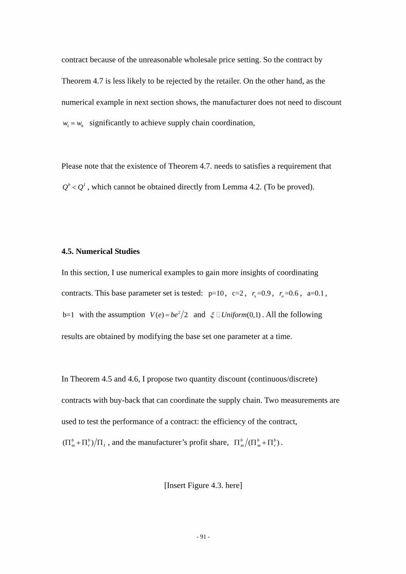
- 91 -
contract because of the unreasonable wholesale price setting. So the contract by
Theorem 4.7 is less likely to be rejected by the retailer. On the other hand, as the
numerical example in next section shows, the manufacturer does not need to discount
1 bw w= significantly to achieve supply chain coordination,
Please note that the existence of Theorem 4.7. needs to satisfies a requirement that
b IQ Q< , which cannot be obtained directly from Lemma 4.2. (To be proved).
4.5. Numerical Studies
In this section, I use numerical examples to gain more insights of coordinating
contracts. This base parameter set is tested: p=10 , c=2 , =0.9sr , =0.6or , a=0.1 ,
b=1 with the assumption 2( ) 2V e be= and (0,1)Uniformξ . All the following
results are obtained by modifying the base set one parameter at a time.
In Theorem 4.5 and 4.6, I propose two quantity discount (continuous/discrete)
contracts with buy-back that can coordinate the supply chain. Two measurements are
used to test the performance of a contract: the efficiency of the contract,
( )b bm r IΠ +Π Π , and the manufacturer’s profit share, ( )b b b
m m rΠ Π +Π .
[Insert Figure 4.3. here]

- 92 -
The above numerical results demonstrate that coordination achieved by the proposed
contracts can improve the supply chain performance significantly. The maximum
efficiency of the buy-back contract and wholesale price contract is around 74% .
Furthermore, the efficiency of the buy-back contract is very robust to parameter
changes because the retailer’s optimal decision on promotional effort is not distorted
through a buy-back credit ob r R= . However, the efficiency of the wholesale price
contract varies as parameter changes due to the fact that neither of retailer’s decisions
have been corrected. As Theorem 4.4. shows, the costliness of effort ( b ) does not
influence the performance of both contracts.
[Insert Figure 4.4. here]
As the figures in 4.4 demonstrate, when the impact of rebate promotion on market
demand is very small, i.e., when parameter a is sufficiently small, the manufacturer
will not issue rebates (it also holds under integrated channel). In this situation, the
buy-back contract becomes wholesale price contract because 0ob r R= = . Furthermore,
The retail price parameter p influences the supply chain in a similar way as the
parameter a does because retail price restricts the upper bound of the rebate value.
Hence, when p is sufficiently small, the impact of a tiny rebate on market demand is
very small and the manufacturer chooses not to issue rebates. Interestingly, there
exists a special relatively small segment for parameters a and p under which the
manufacturer chooses to issue rebates under coordinated channel or uncoordinated

- 93 -
channel with buyback only contract, but not with wholesale price contract. This
implies that the manufacturer with wholesale price only is less likely to offer rebate
promotions. The above figures also show that when rebate benefits are significant, i.e.,
a larger rebate impact ( a ), a higher retail price ( p ), and a higher slippage rate ( s or r ),
the manufacturer’s profit share will increase. For the buy-back contract, the ratio of
optimal rebate value b IR R sticks around 1.04 with very small varying; however, for
the wholesale price contract, w IR R increases with potential rebate benefits.
Moreover, because the rebates help the manufacturer by increasing the order quantity
from the retailer, contrary to general belief, the numerical example suggests that even
if all rebates are redeemed (i.e., by letting 1or = ), the manufacturer would still prefer
providing rebates to consumers as long as neither a nor p is sufficiently small.
[Insert Figure 4.5. here]
The above two figures report the sensitivity of the discrete quantity discount contract
with buy-back based on Theorem 4.7. Without doubt, as the retailer’s profit
reservation parameter λ increases, the manufacturer’s profit share decreases
accordingly. The top figure implies that the proposed contract can achieve supply
chain coordination with arbitrary profit splitting, which is determined by channel
members’ relative bargaining power. Furthermore, the manufacturer does not need to
discount the wholesale price significantly to achieve arbitrary profit splitting. The
bottom figure shows the optimal unit back-back credit ( ob r R= ) decreases with or for

- 94 -
both buy-back only contract and quantity discount contract with buy-back. It is
intuitive that the smaller the probability of redeeming or , the larger the optimal rebate
value R , so the numerical example implies that the optimal R increases at a higher
rate compared to the decreasing rate of or .
4.6. Conclusions
In this chapter, I study a three-way sales promotion that is very popular in practice.
Under the situation where the manufacturer can influence the consumer demand
directly through mail-in rebates while the retailer simultaneously exerts promotional
effort to further spur demand, I find that trade dealing via quantity discounts plus
buy-back is sufficient to coordinate the supply chain. For the deterministic demand
model, even a quantity discount contract itself achieves coordination. The results
show that the performance of a simple wholesale price contract under sales promotion
is not robust and also far from a perfect situation. A successful coordination can result
in significant supply chain improvement, which leads the retailer to order more and
exert higher promotional effort, however, a coordination does not necessarily lead the
manufacturer to issue larger-ticketed rebate.
Hopefully, some of the results in this chapter can provide insights for researchers who
would like to further analyze the coordination issue involving consumer mail-in
rebates. One direct extension is to change the rebate and effort-dependent demand
model to a rebate and price-dependent one. In this case, the retailer can choose the

- 95 -
retail price instead of assuming an exogenously given one. I believe analogous
contracts can coordinate the supply chain if sD ar R bp ξ= + + . An interesting different
game would be to adopt the following timeline of decisions: first the manufacturer
chooses a wholesale price and the retailer determines the order quantity, then the
manufacturer announces the rebate promotion value and the retailer determines the
promotional effort level. Based on this, I can investigate the potential that the
manufacturer uses rebate promotion to coordinate a multiple retailers via structure
coordination. In this scenario, the manufacturer issues rebates which are only valid at
a certain flagship retailer store. Clearly, this rebate promotion will influence the
pricing of other retailers during a relatively long promotion period (consider Google
Checkout discount as an example). Hence, the manufacturer can use this partial
forward integration instead of contracting schemes to improve the performance of a
supply chain. Another line of extension would be to change rebate promotions to the
idea of price match where the retailer price match the price difference to the
customers if the price drops in a short period or the other authorized retailer has a
lower price.
The analytical results are based on a specification of market demand. Other types of
demand functions may generate different managerial insights. Moreover, the
coordination scheme is certainly not unique. Exploration of other possible
coordinating contracts deserves future analysis, especially under a competitive market
environment.

- 96 -
Figure 4.1. An Example of Restricted Rebates Promotion
Figure 4.2. The Layout of Proposed Contracts

- 97 -
Figure 4.3. Numerical Examples of Contract Efficiency

- 98 -
Figure 4.4. Sensitivity Analysis One

- 99 -
Figure 4.5. Sensitivity Analysis Two

- 100 -
CHAPTER 5
RETAILER’S PROMOTIONAL CAMPAIGN: WHY WAL-MART
NEVER ISSUES REBATES

- 101 -
5.1. Brief Introduction
Mail-in rebates have become common promotional techniques in the modern industry.
Given the high slippage rate of rebates, many manufacturers not only have spurred
demand but have also generated free money via rebate promotions. With the recent
rebate boom, many manufacturers have subcontracted the administrative rebate
process to some third-party rebate fulfillment businesses. The popularity of rebates is
not only limited to manufacturers; many retailers also provide their own rebates to
attract consumers. Some retailers, like Staples, have launched paperless rebates
systems to decrease the rebates processing cost and also build customer loyalty.
However, the world’s largest retailer, Wal-Mart, never issues rebates.
The question arising here actually addresses the core of a retailer’s decision making
on promotional strategy. Typically, the retailer has two choices: one is to be an
everyday low price provider, like Wal-Mart; the other is to adopt higher base retail
prices but offer higher promotional discounts. Apparently, everyday low price (EDLP)
has many potential benefits, such as relatively consistent demand, low advertising
cost, and low managerial and inventory cost. Marketing researchers have provided a
variety of reasons to explain the coexistence of EDLP and other promotional
strategies. As a departure from traditional literature on the marketing and operations
interface, which typically involves retail pricing with inventory decisions, in this
chapter I focus on the comparison of two promotion vehicles: rebate promotions and
an EDLP policy under the environment incorporating typical economic order quantity
- 102 -
(EOQ) assumptions.
This chapter show that the retailer’s decision making on promotional strategies
depends upon several factors. Among the most important of these are the demand
price sensitivity and the regular undiscounted retail price on market. I argue that
choices between rebates promotion and EDLP are positioning strategies rather than
purely pricing strategies.
5.2. Model Development
This section describes and formulates the model. For a typical rebate offer, there are
three characteristics: value of the reward, length of the redemption period, and
redemption effort. In my model of characterizing a rebate, I focus on the role of the
rebate face value R and the required redemption effort e . According to the
empirical research of Soman (1998) and Silk (2004), consumers’ purchase decisions
of products offering a rebate can be independent of the decisions to redeem the rebate.
In particular, at the time of purchase, consumers tend to underweight the latent future
redemption effort and be highly confident of redeeming a rebate. Such misperception
of consumers can even be exacerbated by highlighting the reward benefits and not
highlighting the effort required to redeem (Soman 1998, Moorthy and Soman 2003).
So I assume that consumers’ subjective probabilities of redeeming, which determine
their purchase decisions, are only related to the reward size but not related to the

- 103 -
actual redemption effort required. The subjective probability of redeeming sr is
strictly increasing with the rebate face value R , implying that a larger reward
increases the effectiveness of a rebate offer and generates more market demand.
Similar to Soman (1998), I assume a linear deterministic demand, i.e.,
( )( ) ( )R o sD R a b p r R R= − − ⋅ ,
where RD is the consumer demand in the market during the promotional period
op is the regular undiscounted retail price on market
a is the market potential parameter
b is the price sensitivity parameter
( )sr R is the consumer’s subjective probability of redeeming.
In the demand model, ( )o sp r R R− ⋅ can be interpreted as the net effective retail price
including the rebate incentive. Different from Khouja (2006), the retail price op is
not a decision variable in my model but exogenously given, which can be justified
under a sufficiently competitive market where retailers are price takers. Such a
phenomenon is also common in practice where retailers provide rebates but do not
necessarily increase their retail price during the promotional period.
As mentioned previouly, a high redemption confidence does not necessarily translate
into actual redemption behavior (Silk 2004). At the time of redemption, consumers
become more accurately aware of the required redemption effort. Thus, the size of the
reward has a weaker effect on the redemption decisions because consumers reevaluate
the rebate value relative to the extent of required redemption effort. So I assume that

- 104 -
consumers’ objective probabilities of redeeming increases in rebate value R but
strictly declines in required effort level e . In my model, the effort level e is a real
number greater than or equal to 1, which reflects the inherent difficulty level that the
retailer imposes on the redemption of rebate. For example, 1e = might represent a
requirement of only submitting the purchasing information online; 2e = might
represent a requirement of filling out forms and cutting and mailing the original UPC;
while 3e = might require purchase of extra products to qualify for a rebate besides
the regular redemption effort, etc. Rebate slippage is caused by the difference between
consumers’ subjective probabilities of redeeming and their objective probabilities of
redeeming. Apparently, for any given rebate size, a high required redemption effort
can result in a high slippage rate. However, a slippage rate caused by redemption
effort can have an upper limit. So I assume that the consumer’s objective probability
of redeeming, denoted by ( , )or R e is convex, decreasing in e , and ( , 1) ( )o sr R e r R= = .
Furthermore, simple redemption requirement usually has a lower unit rebate
processing cost for the retailer. For example, the processing of a Staples’ easy rebate
does not require any manual work by Staples but processing of a regular mail-in paper
rebate requires a certain level of manual processing or even involves a payment to
some special rebate fulfillment businesses. On the other hand, “experiencing a high
effort redemption process dramatically decreases the proportion of rebate buyers that
purchase the offer again” (Silk, 2004), i.e., a higher effort level hurts the customers’
loyalty. So I build an effort-induced unit cost ( )c e for the retailer. This cost ( )c e is

- 105 -
an overall cost measure, which may include the rebate processing cost, the loss of
future sales, and the damage to the customers’ loyalty in the long run. So I assume
( )c e is convex and increasing in e .
Assuming no supplier capacity constraints, all replenishment orders incur a fixed
setup cost s . In addition, the retailer incurs inventory holding cost which at any point
in time is proportional to its inventory level and the retail price. However, because of
a single-period modeling, the retailer is assumed not to carry inventory from one
promotional season to the next one. Therefore, for a retailer providing rebate
promotion in a certain promotional period, its profit function can be written as
follows:
( )( , , ) ( ) ( , )( ( )) ( )2
Ro R o R oR
D RQR Q e p D R r R e R c e D R hp sQ
= − + − −∏ , (5.1)
where Q is the order quantity
s is the setup cost per order placed by the retailer
h is the inventory holding cost per unit per dollar during the promotional
period.
Instead, if the retailer chooses to adopt a direct price cut, i.e., offering an everyday
low price rather than a rebate promotion, the market demand function and the
retailer’s profit function are
( )P oD a b pλ λ= − ,

- 106 -
( )( , ) ( )2
Po P oP
DQQ p D h p sQλλ λ λ λ= − −∏ , (5.2)
respectively, whereλ is the price reduction percentage.
The logical boundary conditions are listed below:
(A1) 0oa bp− > , which guarantees no negative demand under the undiscounted retail
price even if there is no promotions.
(A2) oR p≤ , 1e ≥ , 1λ ≤
(A3) RD Q≥ or pD Q≥ , which guarantees the order quantity per time will no be
greater than the total market demand during the season.
5.3. Analysis of Rebate Promotions Using Specific Functional Forms of sr , or ,
and ( )c e
To obtain managerial insights, I begin by assuming that ( )s or R R p= , which implies
that consumers’ redemption confidence and the attractiveness of a rebate offer
increases linearly in the ratio of the rebate value R to the regular retail price op of
the product. At the extreme, a free-after-rebate product ( oR p= ) has a 100%
redemption confidence. However, even these 100% rebates do not elicit 100%
redemption because of the redemption effort involved. I further assume that
consumers’ objective probability of redeeming is 1( , )oo
Rr R ep e
= ⋅ . Obviously, there is
no slippage behavior when 1e = in my setting. The unit rebate induced cost ( )c e is

- 107 -
assumed to be 2( ) oc e cp e= , where c is a sufficiently small number and can be
interpreted as the retailer’s costliness parameter of a rebate offer. Under these
assumptions, the retailer’s profit function (5.1) becomes,
2
( )( , , ) ( ) ( , )( ( )) ( )2
( )1( ) ( ) ( )2
Ro R o R oR
Ro R o R o
o
D RQR Q e p D R r R e R c e D R hp sQ
D RR Qp D R R cp e D R hp sp e Q
= − + − −
= − ⋅ + − −
∏
where ( ) ( )R oo
RD R a b p Rp
= − − ⋅ .
By embedding the demand function inside the profit function, the sufficient
conditions for optimality are obtained by taking the first-order derivatives with
respect to Q and e , respectively,
* 2 ( )RR
o
sD RQhp
= (5.3)
*
o
Recp
= (5.4)
For any given rebate value R , we can obtain the following Hessian matrix,
3
3
12 0
2 10o
sDQ
HRDp e
⎡ ⎤− ⋅⎢ ⎥⎢ ⎥=⎢ ⎥− ⋅⎢ ⎥⎣ ⎦
.
So the Hessian matrix is negative definite for any given R .
Furthermore, from (5.4), we can obtain
* **
1( , )oo o
R cRr R e cep e p
= ⋅ = = ,
which implies that for any given R , the consumer’s objective probability of

- 108 -
redeeming is increasing with the optimal redemption effort level. Although this seems
counter-intuitive, the explanation is that the higher the optimal redemption effort level
implies a larger rebate face value, which resulting a higher objective probability of
redeeming.
By embedding (5.3) and (5.4) into the retailer’s profit function, we have
32
32 2 22
( ) ( ) 2 ( ) 2 ( )
( ) 2 ( ) 2 ( ).
o R R o RRo
o o o o oo o o o
cR p D R R D R shp D Rp
b c b bp a bp R R a bp R shp a bp Rp p p p
= − −
= − + − − + − − +
∏
For ( )R R∏ to be concave requires that
2 22
2
( ) 3 35 22 ( ) 1 02 2 ( ) ( )
Ro
o o o R o R
R c b sh bRb a bp R bR p R p p D R p D R
⎛ ⎞ ⎛ ⎞∂= − − + − − ≤⎜ ⎟ ⎜ ⎟∂ ⎝ ⎠ ⎝ ⎠
∏ .
Although the above condition does not hold for all parameter settings, it can be easily
tested that the above condition holds for a wide range of realistic parameter values. So
from the first order condition of R , the optimal rebate value *R should satisfy the
following equation,
1 122 2
2 2
22 3( ) 7 0oo o o o
c b shRR bR a bp R bp p ap bp bR
⎧ ⎫⎛ ⎞⎪ ⎪− − + − =⎨ ⎬⎜ ⎟ − +⎪ ⎪⎝ ⎠⎩ ⎭ (5.5)
Hence, 0R = is a possible candidate for the optimal solution. If the retailer decides
not to offer rebates, the optimal order quantity *Q is given by * 2 ( )o
o
s a bpQhp−
= ,
which leads to a profit of ( ) 2 ( )R o o o op a bp shp a bpΠ = − − − . If the retailer can achieve
higher profits by offering rebates, the optimal rebate face value *R can be solved
from the equation below,
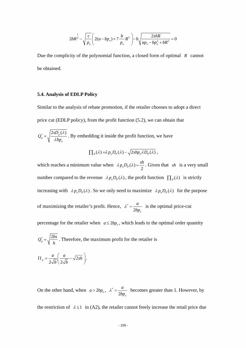
- 109 -
122
2 2
22 2( ) 7 0oo o o o
c b shRbR a bp R bp p ap bp bR
⎛ ⎞− − + − =⎜ ⎟ − +⎝ ⎠
Due the complicity of the polynomial function, a closed form of optimal R cannot
be obtained.
5.4. Analysis of EDLP Policy
Similar to the analysis of rebate promotion, if the retailer chooses to adopt a direct
price cut (EDLP policy), from the profit function (5.2), we can obtain that
* 2 ( )pp
o
sDQ
hpλ
λ= . By embedding it inside the profit function, we have
( ) ( ) 2 ( )o P o PP p D shp Dλ λ λ λ λ= −∏ ,
which reaches a minimum value when ( )2o Pshp Dλ λ = . Given that sh is a very small
number compared to the revenue ( )o Pp Dλ λ , the profit function ( )P λ∏ is strictly
increasing with ( )o Pp Dλ λ . So we only need to maximize ( )o Pp Dλ λ for the purpose
of maximizing the retailer’s profit. Hence, *
2 o
abp
λ = is the optimal price-cut
percentage for the retailer when 2 oa bp≤ , which leads to the optimal order quantity
* 2p
bsQh
= . Therefore, the maximum profit for the retailer is
22 2p
a a shb b⎛ ⎞
Π = −⎜ ⎟⎝ ⎠
.
On the other hand, when 2 oa bp> , *
2 o
abp
λ = becomes greater than 1. However, by
the restriction of 1λ ≤ in (A2), the retailer cannot freely increase the retail price due

- 110 -
to the pressure from his competitors or manufacturers. Due to the concavity of λ , the
retailer chooses not to offer any price-cut promotion, i.e., * 1λ = , which results in a
maximum profit of ( ) 2 ( )p o o o op a bp shp a bpΠ = − − − .
5.5. Sensitivity Analysis and Discussions
In this section, I use numerical examples to gain further insights. Consider a product
with the market potential 20,000a = and price sensitivity 0.02b a= × (i.e., a dollar
change in effective retail price will cause the demand to change by 2% ). The other
parameters in the base set include op =30 , c=0.1 , =0.01h , and =2000s . All the
following analytical results are obtained by modifying the base set by one or two
parameters at a time.
For a linear demand function, the most important parameters are the market potential
a and the price sensitivity b . Previous studies (Gerstner et al. 1994, Moorthy and Lu
2004, Chen et al. 2005) have confirmed that rebate/coupon promotion is an effective
technique for price-discriminating by making products appealing to price-sensitive
consumers. Because of this price sensitivity, the retailer can charge customers
different prices through slippage. My results also imply that rebate promotion is more
effective than direct price-cut promotion (EDLP) when consumers are highly
price-sensitive.

- 111 -
[Insert Table 5.1. here]
[Insert Figure 5.1. here]
Table 5.1 and Figure 5.1 (where b varies from 0.015 a× to 0.025 a× ) show that the
benefits of rebates promotion increases with consumers’ price sensitivity. Some
product categories have low price sensitivity. In this situation, the EDLP promotion is
at least as effective as rebates promotion and retailer chooses not to provide rebates.
Because consumers are not price-sensitive enough, a rebate promotion cannot attract
more customers and generate significant revenue increases to cover the high rebate
promotion costs. In Blattberg and Neslin (1990), the authors argue that frequent
promotion can increase price sensitivity, which is a limitation of promotions. However,
I argue that a product category with high price sensitivity can also be beneficial to the
retailer to implement rebate promotions where the retailer can vary the level of
redemption effort to cause slippage.
The numerical results further suggest that the market potential parameter a plays a
less important role on the choices of promotions. As the Figure 5.2 shows, the benefits
brought by rebate promotions under a high market potential is not as significant as the
benefits under a high price sensitivity. Figure 5.3 shows that the optimal rebate face
value increases with the market potential parameter but at an extremely small rate, i.e.,
the optimal rebate value is insensitive to parameter a .
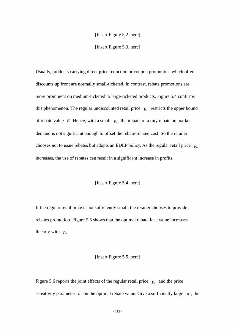
- 112 -
[Insert Figure 5.2. here]
[Insert Figure 5.3. here]
Usually, products carrying direct price reduction or coupon promotions which offer
discounts up front are normally small-ticketed. In contrast, rebate promotions are
more prominent on medium-ticketed to large-ticketed products. Figure 5.4 confirms
this phenomenon. The regular undiscounted retail price op restricts the upper bound
of rebate value R . Hence, with a small op , the impact of a tiny rebate on market
demand is not significant enough to offset the rebate-related cost. So the retailer
chooses not to issue rebates but adopts an EDLP policy. As the regular retail price op
increases, the use of rebates can result in a significant increase in profits.
[Insert Figure 5.4. here]
If the regular retail price is not sufficiently small, the retailer chooses to provide
rebates promotion. Figure 5.5 shows that the optimal rebate face value increases
linearly with op .
[Insert Figure 5.5. here]
Figure 5.6 reports the joint effects of the regular retail price op and the price
sensitivity parameter b on the optimal rebate value. Give a sufficiently large op , the

- 113 -
retailer will choose to offer rebates even at a low value of price sensitivity, i.e., the
profitable range of parameter b for the retailer to offer rebates expands as op
increases.
[Insert Figure 5.6. here]
It should be noted that above the results are based on a reasonable range of values.
For example, if op is extremely large, the retailer tends to issue an extremely big
rebate but at the same time has to require an extraordinarily high redemption effort
level for the purpose of slippage. However, an extremely complicated rebate
redemption process is definitely not welcomed by customers, which will significantly
hurt the customer loyalty and make them avoid products carrying such offers.
Moreover, extremely complicated rebate redemption may also increase the rebate
processing cost and the cost of handling customer’s complaints. All of these
consequences can cause a variation on the retailer’s costliness parameter c of rebate
offer. As c increases, the profitability of a rebate promotion decreases and the
retailer chooses the EDLP instead of rebate promotion. Figure 5.7 and Figure 5.8
show that both the optimal rebate value and optimal redemption effort level decrease
rapidly in the rebate costliness parameter c . At an extreme, if parameter c is
sufficiently small, the retailer may provide free-after-rebate offer, i.e., the optimal
rebate value is equal to the regular price. Such rebate offers are not rare in practice
(see http://www.free-after-rebate.net for examples). For free-after-rebate products,
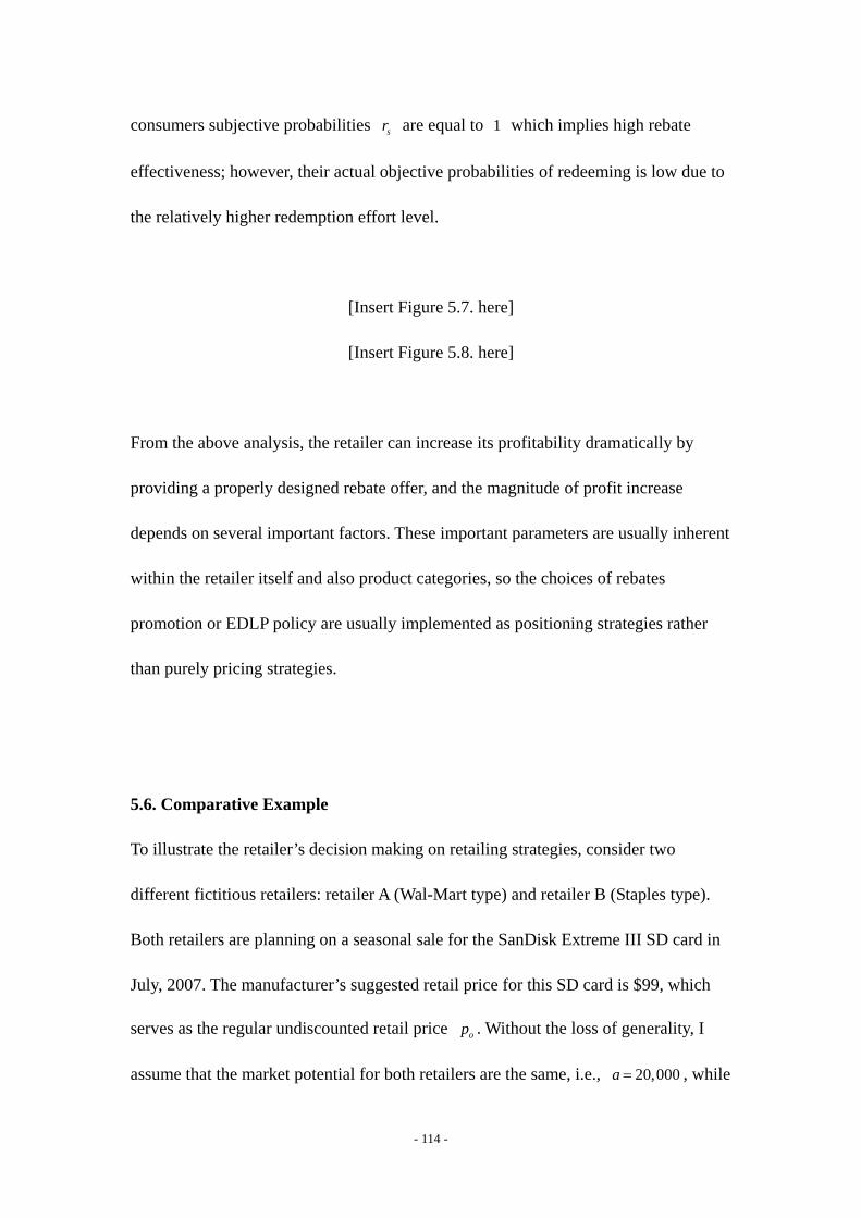
- 114 -
consumers subjective probabilities sr are equal to 1 which implies high rebate
effectiveness; however, their actual objective probabilities of redeeming is low due to
the relatively higher redemption effort level.
[Insert Figure 5.7. here]
[Insert Figure 5.8. here]
From the above analysis, the retailer can increase its profitability dramatically by
providing a properly designed rebate offer, and the magnitude of profit increase
depends on several important factors. These important parameters are usually inherent
within the retailer itself and also product categories, so the choices of rebates
promotion or EDLP policy are usually implemented as positioning strategies rather
than purely pricing strategies.
5.6. Comparative Example
To illustrate the retailer’s decision making on retailing strategies, consider two
different fictitious retailers: retailer A (Wal-Mart type) and retailer B (Staples type).
Both retailers are planning on a seasonal sale for the SanDisk Extreme III SD card in
July, 2007. The manufacturer’s suggested retail price for this SD card is $99, which
serves as the regular undiscounted retail price op . Without the loss of generality, I
assume that the market potential for both retailers are the same, i.e., 20,000a = , while

- 115 -
the price sensitivity parameter b is 0.006 a× and 0.008 a× for retailer A and B,
respectively. Other parameter values are c=0.15 , =0.01h , and =5000s . Thus, the
only difference between the two retailers is the price sensitivity of their respective
customers.
By solving equation (5.5), the optimal rebate values for retailer A and retailer B are
$43.68 and $70.50, respectively. Embedding the rebate values into (5.3) and (5.4), the
optimal solutions using both policies can be obtained as in Table 5.2.
[Insert Table 5.2 here]
From Table 5.2, obviously retailer A should adopt the EDLP policy, while retailer B
should adopt a rebate promotion. Hence, depending on the different values of inherent
marketing parameters, the choices of rebate promotion or EDLP policy are
positioning strategies rather than purely pricing strategies.
5.7. Conclusions
In this chapter, I use an EOQ based model to compare two different promotional
policies: rebate promotion and EDLP via direct price-cut. For rebate promotion, the
retailer needs to jointly determine the optimal order quantity, the rebate face value and
the level of redemption effort. For EDLP, the retailer needs to determine the optimal

- 116 -
order quantity and the price reduction percentage. I show that rebate promotions can
result in a significant increase in profits depending on several important factors, such
as the price sensitivity parameter, the regular undiscounted retail price, and the rebate
costliness parameter. The different values of these factors induce the retailer to make a
choice between rebate promotions and EDLP. Customers visiting Wal-Mart are
typically “expected price shoppers” and are less likely to chase deals all over town
once they are in store. Hence, such customers typically have lower price sensitivity, so
as a positioning strategy Wal-Mart chooses to adopt an EDLP policy. Most of the
products offered at Wal-Mart stores are small-ticketed non-durable goods, which are
not suitable for rebate promotion by my analysis.
Although the rebate face value and required redemption effort play an important role
on consumers’ purchase and redemption behaviors, there are some other factors
contributing to creating slippage behavior which have not been studied in this chapter.
For example, Gourville and Soman (2004) suggests an anchoring and self adjustment,
while Silk (2004) provides procrastination and forgetting as additional explanation for
slippage. Furthermore, the benefits of rebates are not restricted to the increasing
profits brought by slippage. Rebate promotions also provide the retailer interest free
loans during the long redemption and processing period even if customers
successfully receive the rebate checks.
Another limitation in this chapter is the use of a linear demand model, which is not

- 117 -
suitable for extreme values, so future researchers using richer models should be able
to develop more analytical results. Another interesting approach would be to follow
the idea in chapter three and use consumer utility function to generate market demand
and actual redemption rate.
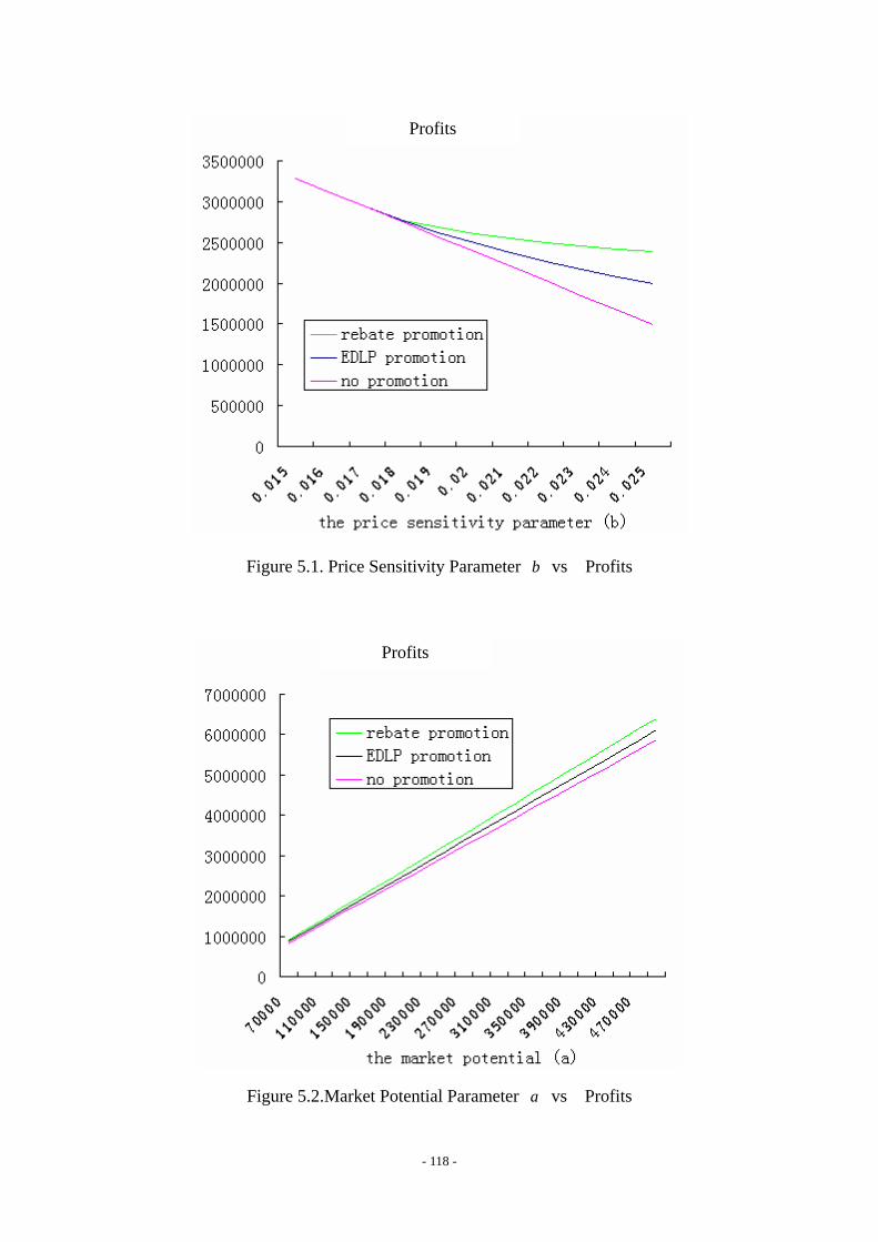
- 118 -
Figure 5.1. Price Sensitivity Parameter b vs Profits
Figure 5.2.Market Potential Parameter a vs Profits
Profits
Profits
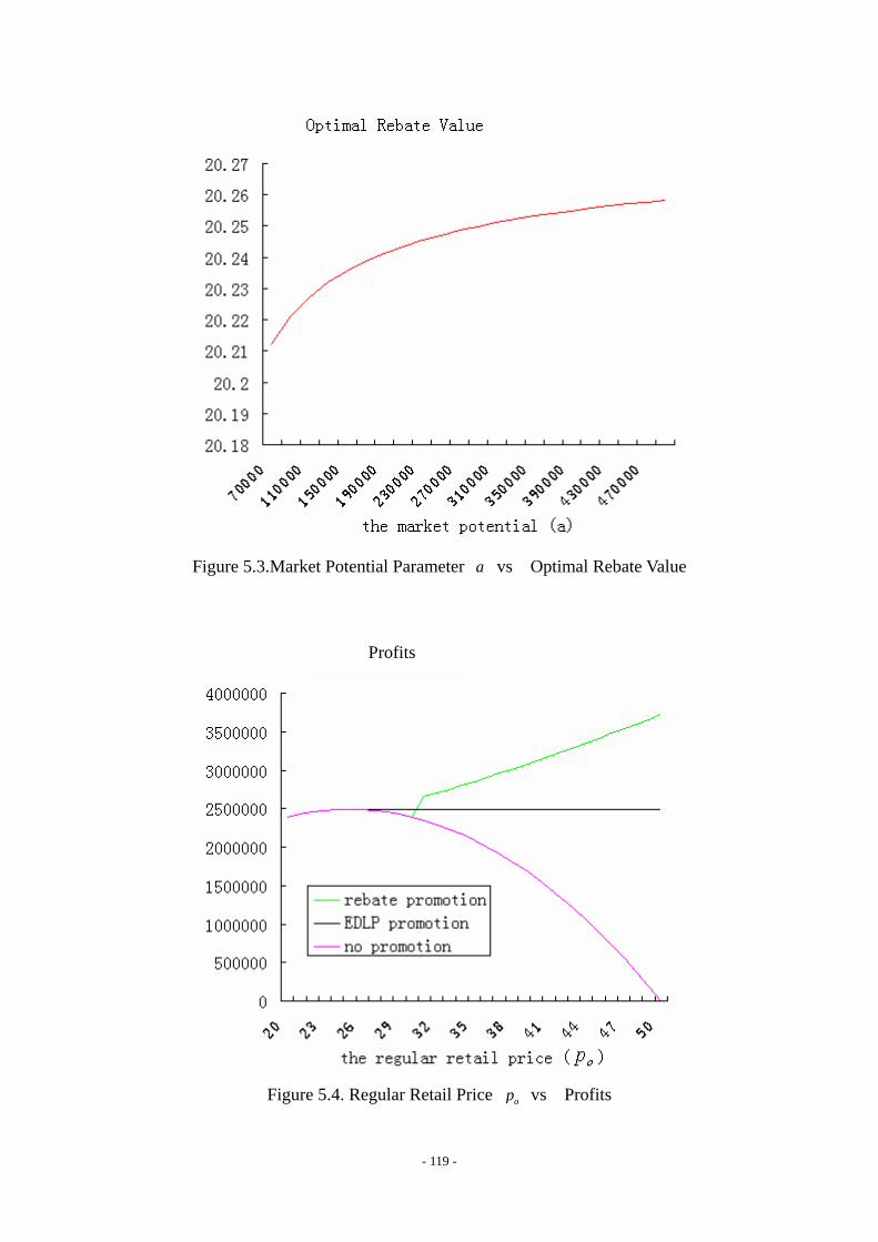
- 119 -
Figure 5.3.Market Potential Parameter a vs Optimal Rebate Value
Figure 5.4. Regular Retail Price op vs Profits
Profits

- 120 -
Figure 5.5. Regular Retail Price op vs Optimal Rebate Value
Figure 5.6. The Joint Effects of Regular Retail Price op and Price Sensitivity
Parameter b

- 121 -
Figure 5.7. Rebate Costliness Parameter c vs Optimal Rebate Value
Figure 5.8. Rebate Costliness Parameter c vs Optimal Redemption Effort Level

- 122 -
b R RΠ pΠ noneΠ 0.015 0 3,288,511 3,288,511 3,288,511 0.016 0 3,108,829 3,108,828 3,108,828 0.017 0 2,929,156 2,930,330 2,929,156 0.018 16.58 2,763,035 2,767,237 2,749,493 0.019 18.72 2,679,694 2,621,319 2,569,841 0.02 20.24 2,610,459 2,490,000 2,390,202
0.021 21.45 2,551,759 2,371,193 2,210,576 0.022 22.44 2,501,396 2,263,192 2,030,966 0.023 23.28 2,457,846 2,164,588 1,851,374 0.024 24.01 2,419,980 2,074,204 1,671,802 0.025 24.64 2,386,930 1,991,056 1,492,254
Table 5.1. Effects of Price Sensitivity Parameter b
RΠ pΠ noneΠ R e sr or λ
Retailer A $788,206 $824,167 $794,914 $43.68 1.715 0.441 0.257 0.842
Retailer B $634,215 $616,875 $405,423 $70.50 2.179 0.712 0.327 0.631
Table 5.2. Optimal Solutions of the Comparative Example

- 123 -
APPENDIX

- 124 -
Proof of Proposition 3.1:
With the demand function, we can proceed in two different cases.
(a) If r sP r R= , the market demand is equal to 1. The retailer’s profit function is given
by ( )( , ) 1r r sw R P w r R w= − ⋅ = −∏ . Hence, for sw r R≤ , ar sP r R= ; otherwise, if
sw r R> , which leads to a negative profit, the retailer will not choose r sP r R= .
(b) If s r sr R P bs r R< < + , The retailer’s profit function is given by
( ) ( )( , , ) ( , ) ( ) r sr r r r r
bs P r Rw R P P w D P R P wbs
− −= − ⋅ = − ⋅∏
Since ( , , )rr w R P∏ is concave in rP , from FOC, we get ( , )2
b sr
bs w r RP w R + += .
This solution is in the relevant interval if s r sr R P bs r R< < + holds, which leads to
2s
s s s sbs w r Rr R bs r R r R bs w bs r R+ +
< < + ⇔ − < < +
Note that the upper bound for w in case a is larger than the lower bound for w in case
b. Obviously, there is an interval for w in which arP and b
rP are both interior
solutions. The retailer’s best interior solution is the one which leads to higher profits.
A comparison of the retailer’s profits in that region shows that
2 2
* ( ) ( )( , ) ( , , ) 04 4s s
r r srbs r R w bs w r Rw R w R P r R w
bs bs+ − + −
− = − − = − ≤∏ ∏ .
Hence, the interior solution is arP for sw r R bs≤ − , and it is b
rP for
s sr R bs w bs r R− < < + .
c) If r sP bs r R≥ + , apparently the retail will not choose this region because of the zero
consumer demand.
From the retailer’s response, the manufacturer chooses his optimal combination of w
and R fore each case.

- 125 -
a) with sw r R bs≤ − , the retailer chooses ar sP r R= and the manufacturer’s profit can
be written as,
0( , ) ( ) 1 ( )m o s s ow R w r R r R bs r R r r R bs= − ⋅ ≤ − − = − −∏
So obviously, there are two cases: s or r= and s or r>
Case a1: If s or r= , which leads to a negative manufacturer’s profit, so the
manufacturer does not have a feasible solution in this interval.
Case a2: If s or r> , the manufacturer’s profit is strictly increasing in R without bound.
The manufacturer’s optimal solution is *sw r R bs= − .
By (A4), *s o
s o
bsw r R bs r R Rr r
= − ≥ ⇔ ≥−
. So if s or r> , ,s o
bsRr r⎡ ⎞
∈ ∞⎟⎢ −⎣ ⎠, which leads to
r sP r R= and sw r R bs= − . Hence, the manufacturer chooses the highest feasible
*R = ∞ , *rP = ∞ and *w = ∞ , which results in a profit of m= ∞∏ .
b) For s sr R bs w bs r R− < < + , given the information that the retailer will choose
( , )2
b sr
bs w r RP w R + += , the manufacturer’s profit function is given by
( )( , ) ( ) ( )2
br s s
m o obs P r R bs w r Rw R w r R w r R
bs bs− − − +
= − ⋅ = − ⋅∏
In order to solve the manufacturer’s problem we proceed in two steps, first, we
characterize the optimal wholesale price, *( )w R , for a given rebate face value R, and
next, we find the optimal R, by embedding *( )w R in the manufacturer’s objective
function and maximizing it over R.
The manufacturer’s objective is concave in w, so from FOC, we get
* ( )( )2s obs r r Rw R + +
= , which is greater than or R . By embedding *( )w R in the
manufacturer’s objective function, the manufacturer’s profit follows as

- 126 -
( ) 2
( )8s o
m
bs r r RR
bs⎡ + − ⎤⎣ ⎦=∏
So obviously, there are two cases: s or r= and s or r>
Case 1: s or r=
It is straightforward to verify that I can get 2obsw r R− = in equilibrium, which is
equivalent to the optimal wholesale price decision.
Case 2: s or r>
Since its profit is strictly increasing in R , the manufacturer will choose the highest
feasible R . From the restriction of relevant region, we have
( ) 32s o
s s s ss o
bs r r R bsr R bs w bs r R r R bs bs r R Rr r
+ +− < < + ⇔ − < < + ⇔ <
−
Hence, the manufacturer chooses the corner solution 3
s o
bsr r−
. However, if the
manufacturer chooses 3
s o
bsRr r
=−
, the retailer will choose r sP r R= , which is the
situation under case a. Hence, if s or r> , the manufacturer does not have a feasible
solution for the interval s sr R bs w bs r R− < < + .

- 127 -
Proof of Lemma 3.1.: Being confronted with the four intervals of the demand function
( , , )r sD P R P , the retailer chooses the optimal ( , , )r sP w R P for any given w , R and
sP of the manufacturer.
a) For 1
s sr
r R PP αα
+≤
+, the retailer’s optimal retail price is straightforward,
1a s s
rr R PP α
α+
=+
for 1
s sr R Pw αα
+≤
+
Otherwise, if 1
s sr R Pw αα
+>
+, which leads to negative profits, the retailer will not
choose rP in this interval.
b) For 1
s sr s
r R P P Pαα
+< ≤
+, the retailer’s profit function is given by
( ) (1 )( ) r s sr r r
bs P r R PP P wbs
α α− + + +⎛ ⎞= − ⎜ ⎟⎝ ⎠
∏
The above objective is concave in rP , so from FOC, we get
2 2(1 )b s s
rbs r R PwP α
α+ +
= ++
This solution is in the relevant interval if 1
s sr s
r R P P Pαα
+< ≤
+ holds, which leads to
1 2 2(1 ) 1 1s s s s s s s s
s sr R P bs r R P P r R bs r R bs Pw P w Pα α α
α α α α+ + + + − + −
< + ≤ ⇔ < ≤ −+ + + +
Note that the upper bound for w in case a is greater than the lower bound for w in case
b. Obviously, there is an interval for w in which ( )arP R and ( , )b
rP w R are bother
interior solutions. The retailer’s best interior solution is the one which leads to higher
profits. A comparison of the retailer’s profits in that region shows that
21( , ) ( , ) ((1 ) ) 04(1 )
a br r r r s sw P w P w bs r R P
bsα α
α− = − + + − − ≤
+∏ ∏
Hence, the interior solution is arP for
1s sP r R bsw α
α+ −
≤+
, and it is brP for
1 1s s s s
sP r R bs r R bs Pw Pα
α α+ − + −
< ≤ −+ +
.

- 128 -
c) For 1
s ss r
bs r R PP P ββ
+ +< <
+, the retailer’s maximization function is
( ) (1 )( ) r s sr r r
bs P r R PP P wbs
β β− + + +⎛ ⎞= − ⎜ ⎟⎝ ⎠
∏
The above objective is concave in rP , so from FOC, we have
2 2(1 )c s s
rbs r R PwP β
β+ +
= ++
This solution is in the relevant interval if 1
s ss r
bs r R PP P ββ
+ +< ≤
+ holds, which leads
to
2 2(1 ) 1 1 1s s s s s s s s
s sbs r R P bs r R P r R bs P P r R bswP P wβ β β
β β β β+ + + + + − + +
< + < ⇔ − < <+ + + +
From (A6), we have sw P≤ . Since the RHS 1 1
s s s ss
P r R bs P P Pβ ββ β
+ + +≥ =
+ +, so the
appropriate interval is 1
s ss s
r R bs PP w Pβ
+ −− < ≤
+.
Note that the upper bound for w in case a is always less than the upper bound for w in
case c: by (A6), it is easy to show 1
s ss
r R P Pαα
+≤
+; however, for the upper bound for w
in case a and the lower bound for w in case c the following relation holds:
1 1s s s s
sr R bs P r R PP α
β α+ − +
− ≤+ +
⇔1
2s sP bs r Rαα β+
≤ ++ +
So when 12s sP bs r Rα
α β+
≤ ++ +
, there is an interval for w in which arP and c
rP are
bother interior solutions. The retailer’s best interior solution is the one which leads to
higher profits. A comparison of the retailer’s profits in that region shows that
2
2
( , ) ( , )1( ) ( ) ((1 ) )
1 1 4(1 )( )( ) 1 ((1 ) ) 0
(1 )(1 ) 4(1 )
a cr r r r
s s s ss s
s ss s
w P w Pr R P r R Pw w w bs r R P
bsP r R w bs r R P
bs
α ββ β
α β ββ α
β βα β β
−+ +
= − − − − + + − −+ + +− −
= − − + + − − ≤+ + +
∏ ∏
Hence, the interior solution is crP for
1s s
s sr R bs PP w P
β+ −
− < ≤+
.
d) Since we assume β α> , the upper bound for w in case b is less than the lower

- 129 -
bound in case c. So there exists an interval 1 1
s s s ss s
r R bs P r R bs PP w Pα β
+ − + −− ≤ ≤ −
+ + for
which dr sP P= is a corner solution to the retailer’s optimization problem.
Note that for the upper bound for w in case a and the lower bound for w in case d the
following relation holds:
1 1 2s s s s
s s sr R bs P r R P bsP P r Rα
α α+ − +
− ≤ ⇔ ≤ ++ +
So when 2s sbsP r R≤ + , there is an interval for w in which a
rP and drP are bother
interior solutions. The retailer’s best interior solution is the one which leads to higher
profits. A comparison of the retailer’s profits in that region shows that
( )2
( , ) ( , ) ( )1
( )1 1( )( ) ( )( / ) 01 1 1 (1 )
a d s s s sr r r r s
s s s s ss s s s
r R P bs P r Rw P w P w P wbs
P w r R bs P P r RP r R P r R bsbs bs
αα
α α α α
+ − +⎛ ⎞− = − − − ⎜ ⎟+ ⎝ ⎠− + − −
= − − ≤ − − = − ≤+ + + +
∏ ∏
Hence, the interior solution is drP for
1 1s s s s
s sr R bs P r R bs PP w P
α β+ − + −
− < ≤ −+ +
e) For 1
s sr
bs r R PP ββ
+ +≥
+, obviously the retailer does not have a feasible rP from this
interval with zero consumer demand.
f) Now that all interior solutions are calculated, we have to compare the retailer’s
profits associated with those solutions to the profits at the corner of the intervals. It is
straightforward to exclude 0rP = and 1
s sr
bs r R PP ββ
+ +=
+ as optimal retail prices for
any combination ( , , )sw R P of the manufacturer because both cannot lead to positive
profits for the retailer.
First consider arP for
1s sP r R bsw α
α+ −
≤+
. Only r sP P= is a candidate for corner
solution. A comparison of profits shows that

- 130 -
2
1( , ) ( , ) ( )( )1
( )1( )(( ) / ) 01 1 (1 )
a sr r r r s s s
s s s ss s s
P ww P w P P P r Rbs
P r R bs P r RP r R P bsbs
αα
α α α
−− = = − −
++ − −
≥ − − − = ≥+ + +
∏ ∏
Hence, if 1
o sp r R bsw αα
+ −≤
+, the retailer still chooses a
rP .
Next consider brP for
1 1s s s s
sP r R bs r R bs Pw Pα
α α+ − + −
< < −+ +
. The only possible
candidate 1
s sr
bs r R PP ββ
+ +=
+ as a corner solution is already excluded.
Next consider drP for
1 1s s s s
s sr R bs P r R bs PP w P
α β+ − + −
− ≤ ≤ −+ +
. As we already show in
case d), for the candidate1
s sr
r R PP αα
+=
+ as a corner solution,
( , ) ( , ) 01
ds sr r r r
r R Pw P w Pαα
+= − ≤
+∏ ∏ . Hence, if
1 1s s s s
s sr R bs P r R bs PP w P
α β+ − + −
− ≤ ≤ −+ +
,
the retailer still chooses drP .
Next consider crP for
1s s
s sr R bs PP w P
β+ −
− < ≤+
. As we already show in case c), for
the candidate 1
s sr
r R PP αα
+=
+ as a corner solution,
( , ) ( , ) 01
cs sr r r r
r R Pw P w Pαα
+= − ≤
+∏ ∏ . Hence, if
1s s
s sr R bs PP w P
β+ −
− < ≤+
, the retailer
still chooses crP .
Also, it is straightforward to show that ( )1
a s sr
r R PP R αα
+=
+ is less than or equal to sP
from (A6). The retailer chooses brP when
1 1s s s s
sP r R bs r R bs Pw Pα
α α+ − + −
< < −+ +
, so we
have 2 2(1 ) 2 2(1 ) 2(1 )
b s s s s s s sr s
bs r R P P r R bs P bs r R PwP Pα αα α α
+ + + − + += + < − + =
+ + +.
And, the retailer chooses For crP when
1s s
s sr R bs PP w P
β+ −
− < ≤+
, so we have
2 2(1 ) 2 2(1 ) 2(1 )c s s s s s s s
r sbs r R P P r R bs P bs r R PwP Pβ β
β β β+ + + − + +
= + > − + =+ + +
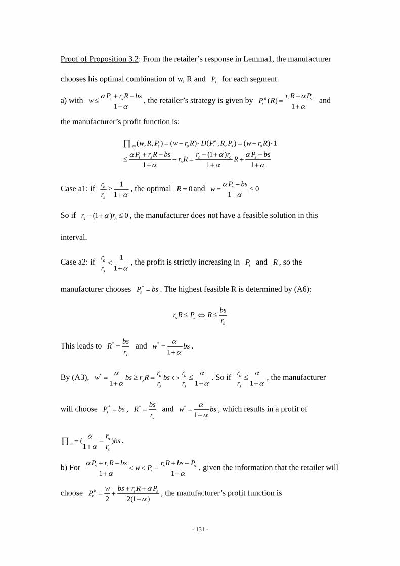
- 131 -
Proof of Proposition 3.2: From the retailer’s response in Lemma1, the manufacturer
chooses his optimal combination of w, R and sP for each segment.
a) with 1
s sP r R bsw αα
+ −≤
+, the retailer’s strategy is given by ( )
1a s s
rr R PP R α
α+
=+
and
the manufacturer’s profit function is:
( , , ) ( ) ( , , ) ( ) 1(1 )
1 1 1
am s o r s o
s s s o so
w R P w r R D P R P w r RP r R bs r r P bsr R Rα α α
α α α
= − ⋅ = − ⋅+ − − + −
≤ − = ++ + +
∏
Case a1: if 11
o
s
rr α≥
+, the optimal 0R = and 0
1sP bsw αα−
= ≤+
So if (1 ) 0s or rα− + ≤ , the manufacturer does not have a feasible solution in this
interval.
Case a2: if 11
o
s
rr α<
+, the profit is strictly increasing in sP and R , so the
manufacturer chooses *sP bs= . The highest feasible R is determined by (A6):
s ss
bsr R P Rr
≤ ⇔ ≤
This leads to *
s
bsRr
= and *
1w bsα
α=
+.
By (A3), *
1 1o o
os s
r rw bs r R bsr r
α αα α
= ≥ = ⇔ ≤+ +
. So if 1
o
s
rr
αα
≤+
, the manufacturer
will choose *sP bs= , *
s
bsRr
= and *
1w bsα
α=
+, which results in a profit of
( )1
om
s
r bsr
αα
= −+
∏ .
b) For 1 1
s s s ss
P r R bs r R bs Pw Pαα α
+ − + −< < −
+ +, given the information that the retailer will
choose 2 2(1 )
b s sr
bs r R PwP αα
+ += +
+, the manufacturer’s profit function is
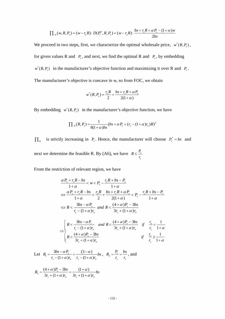
- 132 -
(1 )( , , ) ( ) ( , , ) ( )2
b s sm s o r s o
bs r R P ww R P w r R D P R P w r Rbs
α α+ + − += − ⋅ = − ⋅∏
We proceed in two steps, first, we characterize the optimal wholesale price, *( , )sw R P ,
for given values R and sP , and next, we find the optimal R and sP , by embedding
*( , )sw R P in the manufacturer’s objective function and maximizing it over R and sP .
The manufacturer’s objective is concave in w, so from FOC, we obtain
*( , )2 2(1 )o s s
sr R bs r R Pw R P α
α+ +
= ++
By embedding *( , )sw R P in the manufacturer’s objective function, we have
21( , ) ( ( (1 ) ) )8(1 )m s s s oR P bs P r r R
bsα α
α= + + − +
+∏
m∏ is strictly increasing in sP . Hence, the manufacturer will choose *sP bs= and
next we determine the feasible R. By (A6), we have s
s
PRr
≤
From the restriction of relevant region, we have
1 1
1 2 2(1 ) 13 (4 ) 3
(1 ) 3 (1 )
s s s ss
s s o s s s ss
s s
s o s o
P r R bs r R bs Pw P
P r R bs r R bs r R P r R bs PP
bs P P bsR and Rr r r r
αα α
α αα α α
α αα α
+ − + −< < −
+ ++ − + + + −
⇔ < + < −+ + +
− + −⇔ < <
− + + +
3 (4 ) 3 1(1 ) 3 (1 ) 1
(4 ) 3 13 (1 ) 1
s s o
s o s o s
s o
s o s
bs P P bs rR and R ifr r r r r
P bs rR ifr r r
α αα α α
αα α
− + −⎧ < < <⎪ − + + + +⎪⇒ ⎨ + −⎪ < ≥⎪ + + +⎩
Let 13 (3 )
(1 ) (1 )s
s o s o
bs PR bsr r r r
α αα α
− −= =
− + − +, 2
s
s s
P bsRr r
= = , and
3(4 ) 3 (1 )3 (1 ) 3 (1 )
s
s o s o
P bsR bsr r r rα α
α α+ − +
= =+ + + +
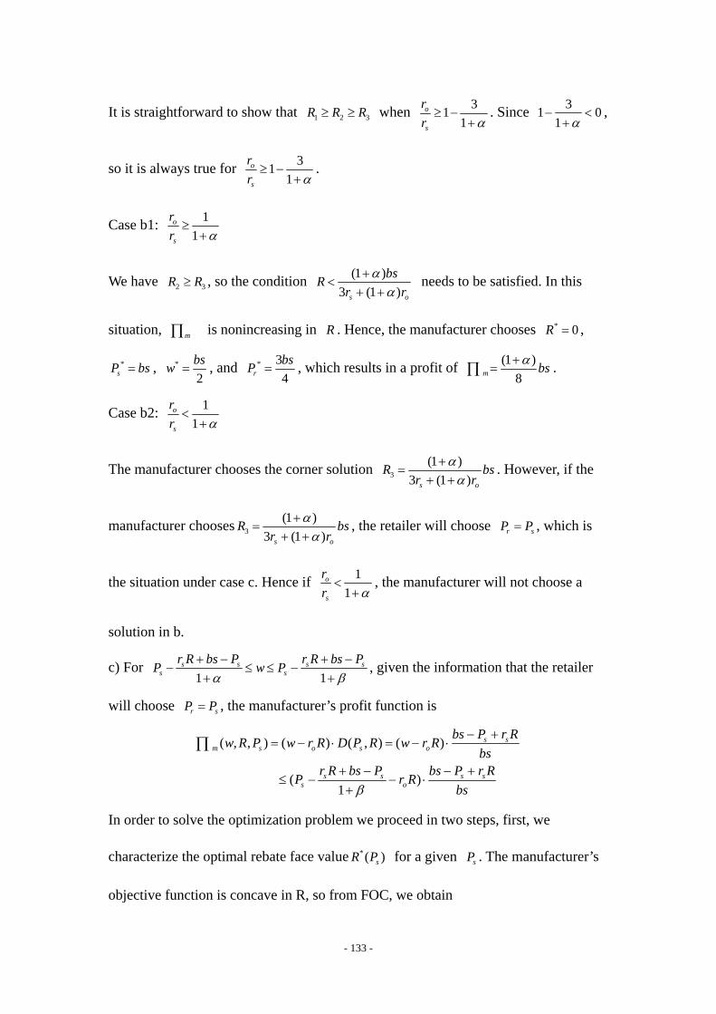
- 133 -
It is straightforward to show that 1 2 3R R R≥ ≥ when 311
o
s
rr α≥ −
+. Since 31 0
1 α− <
+,
so it is always true for 311
o
s
rr α≥ −
+.
Case b1: 11
o
s
rr α≥
+
We have 2 3R R≥ , so the condition (1 )3 (1 )s o
bsRr r
αα
+<
+ + needs to be satisfied. In this
situation, m∏ is nonincreasing in R . Hence, the manufacturer chooses * 0R = ,
*sP bs= , *
2bsw = , and * 3
4rbsP = , which results in a profit of (1 )
8m bsα+=∏ .
Case b2: 11
o
s
rr α<
+
The manufacturer chooses the corner solution 3(1 )
3 (1 )s o
R bsr r
αα
+=
+ +. However, if the
manufacturer chooses 3(1 )
3 (1 )s o
R bsr r
αα
+=
+ +, the retailer will choose r sP P= , which is
the situation under case c. Hence if 11
o
s
rr α<
+, the manufacturer will not choose a
solution in b.
c) For 1 1
s s s ss s
r R bs P r R bs PP w Pα β
+ − + −− ≤ ≤ −
+ +, given the information that the retailer
will choose r sP P= , the manufacturer’s profit function is
( , , ) ( ) ( , ) ( )
( )1
s sm s o s o
s s s ss o
bs P r Rw R P w r R D P R w r Rbs
r R bs P bs P r RP r Rbsβ
− += − ⋅ = − ⋅
+ − − +≤ − − ⋅
+
∏
In order to solve the optimization problem we proceed in two steps, first, we
characterize the optimal rebate face value *( )sR P for a given sP . The manufacturer’s
objective function is concave in R, so from FOC, we obtain
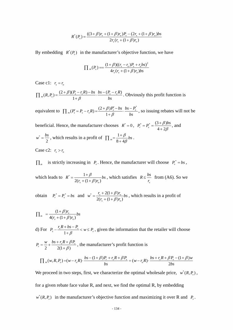
- 134 -
* ((3 ) (1 ) ) (2 (1 ) )( )2 ( (1 ) )
s o s s os
s s o
r r P r r bsR Pr r r
β β ββ
+ + + − + +=
+ +
By embedding *( )sR P in the manufacturer’s objective function, we have
2(1 )(( ) )( )4 ( (1 ) )
s o s om s
s s o
r r P r bsPr r r bsβ
β+ − +
==+ +
∏
Case c1: s or r=
(2 )( ) ( )( , )1
s s s sm s
P r R bs bs P r RR Pbs
ββ
+ − − − −= ⋅
+∏ . Obviously this profit function is
equivalent to (2 )( )1
s sm s s s
P bs bs PP P r Rbs
ββ
′′+ − −′ = − = ⋅+
∏ , so issuing rebates will not be
beneficial. Hence, the manufacturer chooses * 0R = , * * (3 )4 2r s
bsP P ββ
+= =
+, and
*
2bsw = , which results in a profit of 1
8 4m bsββ
+=
+∏ .
Case c2: s or r>
m∏ is strictly increasing in sP . Hence, the manufacturer will choose *sP bs= ,
which leads to * 12( (1 ) )s o
R bsr r
ββ
+=
+ +, which satisfies
s
bsRr
≤ from (A6). So we
obtain * *r sP P bs= = and * 2(1 )
2( (1 ) )s o
s o
r rw bsr r
ββ
+ +=
+ +, which results in a profit of
(1 )4( (1 ) )
sm
s o
r bsr r
ββ
+=
+ +∏
d) For 1
s ss s
r R bs PP w Pβ
+ −− < ≤
+, given the information that the retailer will choose
2 2(1 )s s
rbs r R PwP β
β+ +
= ++
, the manufacturer’s profit function is
(1 ) (1 )( , , ) ( ) ( )2
r s s s sm s o o
bs P r R P bs r R P ww R P w r R w r Rbs bs
β β β β− + + + + + − += − ⋅ = − ⋅∏
We proceed in two steps, first, we characterize the optimal wholesale price, *( , )sw R P ,
for a given rebate face value R, and next, we find the optimal R, by embedding
*( , )sw R P in the manufacturer’s objective function and maximizing it over R and sP .
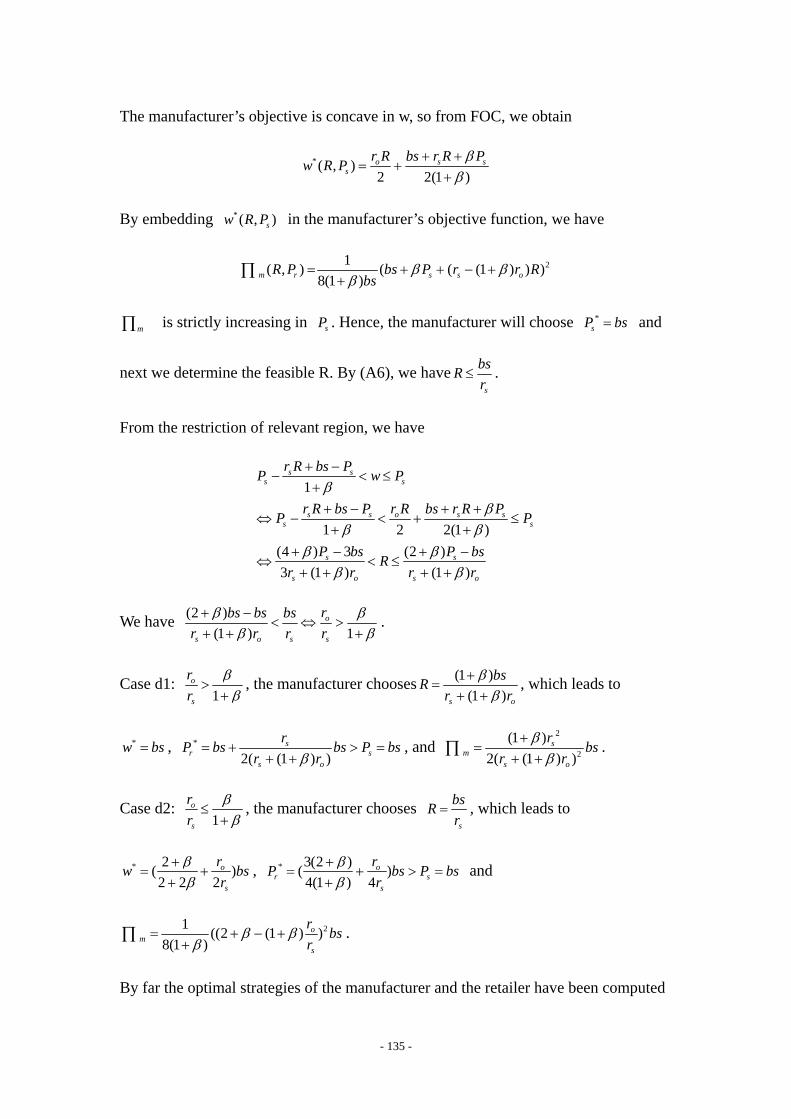
- 135 -
The manufacturer’s objective is concave in w, so from FOC, we obtain
*( , )2 2(1 )o s s
sr R bs r R Pw R P β
β+ +
= ++
By embedding *( , )sw R P in the manufacturer’s objective function, we have
21( , ) ( ( (1 ) ) )8(1 )m r s s oR P bs P r r R
bsβ β
β= + + − +
+∏
m∏ is strictly increasing in sP . Hence, the manufacturer will choose *sP bs= and
next we determine the feasible R. By (A6), we haves
bsRr
≤ .
From the restriction of relevant region, we have
1
1 2 2(1 )(4 ) 3 (2 )3 (1 ) (1 )
s ss s
s s o s ss s
s s
s o s o
r R bs PP w P
r R bs P r R bs r R PP P
P bs P bsRr r r r
ββ
β ββ β
β β
+ −− < ≤
++ − + +
⇔ − < + ≤+ +
+ − + −⇔ < ≤
+ + + +
We have (2 )(1 ) 1
o
s o s s
rbs bs bsr r r r
β ββ β
+ −< ⇔ >
+ + +.
Case d1: 1
o
s
rr
ββ
>+
, the manufacturer chooses (1 )(1 )s o
bsRr r
ββ
+=
+ +, which leads to
*w bs= , *
2( (1 ) )s
r ss o
rP bs bs P bsr rβ
= + > =+ +
, and 2
2
(1 )2( (1 ) )
sm
s o
r bsr r
ββ
+=
+ +∏ .
Case d2: 1
o
s
rr
ββ
≤+
, the manufacturer chooses s
bsRr
= , which leads to
* 2( )2 2 2
o
s
rw bsr
ββ
+= +
+, * 3(2 )( )
4(1 ) 4o
r ss
rP bs P bsr
ββ
+= + > =
+ and
21 ((2 (1 ) )8(1 )
om
s
r bsr
β ββ
= + − ++
∏ .
By far the optimal strategies of the manufacturer and the retailer have been computed

- 136 -
for every interval.
[Insert Table A.1. here]
A comparison of the resulting profits helps to decide which strategy the manufacturer
will eventually to be chosen. Based on the conditions for each candidate strategy set,
we draw the following figure to help visualize the potential candidate sets.
[Insert Figure A.1. here]
First, consider the situation where o sr r= , i.e. no slippage phenomenon, issuing
rebates will not help the manufacturer to improve sales or profits. Both cases b1, c1
and d1 satisfies the condition, so we need to compare the manufacturer’s profits.
1 12
(1 ) 1 1 1 1( ) 02(2 ) 4(2 ) 2(2 ) 2 2
d cm m bs bs bsβ β β
β β β β+ + +
− = ⋅ − = − <+ + + +
∏ ∏
2 21 1
2 2
(1 ) 1 (2 ) 02(2 ) 8 8(2 )
d bm m bs bs bsβ α β α β
β β+ + + +
− = ⋅ − = − <+ +
∏ ∏
1 1 1 1 208 4(2 ) 1
b cm m bs bsα β αβ
β α+ +
− = − ≤ ⇔ ≥+ −
∏ ∏
So if 21αβα
≥−
, the manufacturer will choose strategy set c1; otherwise he will
choose b1.
Next, consider the situation where 1 11
o
s
rrα
≤ <+
, we need to compare cases b1, c2,
and d1.
21 1
2
(1 ) 1 2 102( (1 ) ) 8 1(1 )(1 )
d b s om m
s o s
r rbs bsr r r
β αβ βα β
+ +− = ⋅ − = ≤ ⇔ ≥ −
+ + ++ +∏ ∏
Since 2 1 11 1(1 )(1 ) β αα β
− ≤+ ++ +
, so case b1 dominates case d1 when
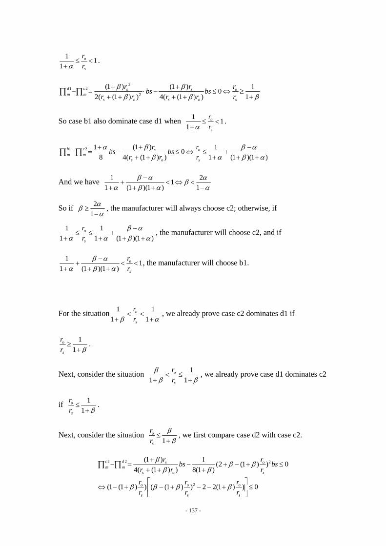
- 137 -
1 11
o
s
rrα
≤ <+
.
21 2
2
(1 ) (1 ) 102( (1 ) ) 4( (1 ) ) 1
d c s s om m
s o s o s
r r rbs bsr r r r r
β ββ β β
+ +− = ⋅ − ≤ ⇔ ≥
+ + + + +∏ ∏
So case b1 also dominate case d1 when 1 11
o
s
rrα
≤ <+
.
1 2 (1 )1 108 4( (1 ) ) 1 (1 )(1 )
b c s om m
s o s
r rbs bsr r r
βα β αβ α β α
++ −− = − ≤ ⇔ ≤ +
+ + + + +∏ ∏
And we have 1 211 (1 )(1 ) 1
β α αβα β α α
−+ < ⇔ <
+ + + −
So if 21αβα
≥−
, the manufacturer will always choose c2; otherwise, if
1 11 1 (1 )(1 )
o
s
rr
β αα α β α
−≤ ≤ +
+ + + +, the manufacturer will choose c2, and if
1 11 (1 )(1 )
o
s
rr
β αα β α
−+ < <
+ + +, the manufacturer will choose b1.
For the situation 1 11 1
o
s
rrβ α
< <+ +
, we already prove case c2 dominates d1 if
11
o
s
rr β≥
+.
Next, consider the situation 11 1
o
s
rr
ββ β< ≤
+ +, we already prove case d1 dominates c2
if 11
o
s
rr β≤
+.
Next, consider the situation 1
o
s
rr
ββ
≤+
, we first compare case d2 with case c2.
2 2 2
2
(1 ) 1 (2 (1 ) ) 04( (1 ) ) 8(1 )
(1 (1 ) ) ( (1 ) ) 2 2(1 ) ) 0
c d s om m
s o s
o o o
s s s
r rbs bsr r r
r r rr r r
ββ β
β β
β β β β
+− = − + − + ≤
+ + +
⎡ ⎤⇔ − + − + − − + ≤⎢ ⎥
⎣ ⎦
∏ ∏
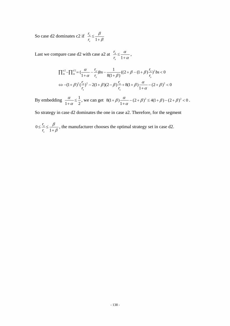
- 138 -
So case d2 dominates c2 if 1
o
s
rr
ββ
≤+
Last we compare case d2 with case a2 at 1
o
s
rr
αα
≤+
,
2 2 2
2 2 2
1( ) ((2 (1 ) ) 01 8(1 )
(1 ) ( ) 2(1 )(2 ) 8(1 ) (2 ) 01
a d o om m
s s
o o
s s
r rbs bsr r
r rr r
α β βα β
αβ β β β βα
− = − − + − + <+ +
⇔ − + − + − + + − + <+
∏ ∏
By embedding 11 2αα≤
+, we can get 2 28(1 ) (2 ) 4(1 ) (2 ) 0
1αβ β β βα
+ − + ≤ + − + <+
.
So strategy in case d2 dominates the one in case a2. Therefore, for the segment
01
o
s
rr
ββ
≤ ≤+
, the manufacturer chooses the optimal strategy set in case d2.

- 139 -
Proof of Proposition 3.4:
For the centralized channel, where the manufacturer owns the retailer, the
manufacturer chooses his optimal combination of ( , , )r sP R P for each segment of the
kinked demand function.
(a) For 1
s sr
r R PP αα
+≤
+, the manufacturer’s profit function is:
(1 )( , , ) ( ) 11 1 1
s s s o sm r s r o o
r R P r r PP R P P r R r R Rα α αα α α
+ − += − ⋅ ≤ − = +
+ + +∏
Case a1: if 11
o
s
rr α≥
+, the optimal * 0R = , *
1rP bsαα
=+
and *sP bs= , which results
in a profit 1m bsα
α=
+∏ .
Case a2: if 11
o
s
rr α<
+, the profit is strictly increasing in sP and R , so the
manufacturer chooses *sP bs= . The highest feasible R is determined by (A6):
s ss
bsr R P Rr
≤ ⇔ ≤
This leads to *
s
bsRr
= and *rP bs= , which results in a profit
(1 ) (1 )1 1
s o om
s s
r r rbs bs bsr r
α αα α
− += ⋅ + = −
+ +∏
(b) For 1
s sr s
r R P P Pαα
+< <
+, the manufacturer’s profit function is
(1 )( , , ) ( ) ( , , ) ( )b r s sm r s r o r s r o
bs P r R PP R P P r R D P R P P r Rbs
α α− + + += − ⋅ = − ⋅∏
We proceed in two steps, first, we characterize the optimal retail price, *( , )r sP R P , for
given values R and sP , and next, we find the optimal R and sP , by embedding
*( , )r sP R P in the manufacturer’s objective function and maximizing it over R and sP .
The manufacturer’s objective is concave in rP , so from FOC, we obtain

- 140 -
*( , )2 2(1 )o s s
r sr R bs r R PP R P α
α+ +
= ++
By embedding *( , )r sP R P in the manufacturer’s objective function, we have
21( , ) ( ( (1 ) ) )4(1 )m s s s oR P bs P r r R
bsα α
α= + + − +
+∏
m∏ is strictly increasing in sP . Hence, the manufacturer will choose sP bs= and
next we determine the feasible R. By (A6), we have s
s
PRr
≤
From the restriction of relevant region, we have
1
1 2 2(1 )(2 ) 1
(1 ) (1 ) 1(2 ) 1
(1 ) 1
s sr s
s s o s ss
s s o
s o s o s
s o
s o s
r R P P P
r R P r R bs r R P P
bs P P bs rR and R ifr r r r r
P bs rR ifr r r
αα
α αα α
α αα α α
αα α
+< <
++ + +
⇔ < + <+ +
− + −⎧ < < <⎪ − + + + +⎪⇒ ⎨ + −⎪ < ≥⎪ + + +⎩
Let 1(1 )
(1 ) (1 )s
s o s o
bs P bsRr r r r
α αα α
− −= =
− + − +, 2
s
s s
P bsRr r
= = , and
3(2 ) (1 )
(1 ) (1 )s
s o s o
P bs bsRr r r r
α αα α
+ − += =
+ + + +
It is straight forward to show that 1 2 3R R R≥ ≥ when 1
o
s
rr
αα
≥+
.
Case b1: 11
o
s
rr α≥
+
We have 2 3R R≥ , so the condition (1 )(1 )s o
bsRr r
αα
+<
+ + needs to be satisfied. In this
situation, m∏ is nonincreasing in R . Hence, the manufacturer chooses * 0R = ,
*sP bs= and *
2rbsP = , which results in a profit of (1 )
4m bsα+=∏ .

- 141 -
Case b2: 11 1
o
s
rr
αα α≤ <
+ +
In this situation, m∏ strictly increasing in R and 1 2 3R R R≥ ≥ . So the
manufacturer chooses the corner solution 3(1 )
(1 )s o
bsRr r
αα
+=
+ +. However, if the
manufacturer chooses 3(1 )
(1 )s o
bsRr r
αα
+=
+ +, we have r sP P= , which is the case under c.
Hence, if 11 1
o
s
rr
αα α≤ <
+ +, the manufacturer does not have a feasible solution in case
b.
Case b3: 1
o
s
rr
αα
<+
In this situation, m∏ strictly increasing in R and 1 2 3R R R< < . So the
manufacturer chooses the corner solution 1(1 )
(1 )s o
bsRr r
αα
−=
− +. However, if the
manufacturer chooses 1(1 )
(1 )s o
bsRr r
αα
−=
− +, we have 1D = , which is the case under a.
Hence, if 1
o
s
rr
αα
<+
, the manufacturer does not have a feasible solution in case b.
(c) For r sP P= , the manufacturer’ profit function is
( , ) ( ) s sm s s o
bs P r RR P P r Rbs
− += − ⋅∏
In order to solve the optimization problem we proceed in two steps, first, we
characterize the optimal rebate face value *( )sR P for a given sP . The manufacturer’s
objective function is concave in R, so from FOC, we obtain
( )* ( )2
s o s os
o s
r r P r bsR P
r r+ −
=
By embedding *( )sR P in the manufacturer’s objective function, we have

- 142 -
( )2( )( )
4s o s o
m so s
r r P r bsP
r r bs− +
=∏
Case c1: s or r=
( )( , ) ( ) s sm s s s
bs P r RR P P r Rbs
− −= − ⋅∏ . Obviously this profit function is equivalent to
( ) sm s s s s
bs PP P r R Pbs
′−′ ′= − = ⋅∏ , so issuing rebates will not be beneficial. Hence, the
manufacturer chooses * 0R = and * *
2r sbsP P= = , which results in a profit of
4mbs
=∏ .
Case c2: s or r>
m∏ is strictly increasing in sP . Hence, the manufacturer will choose *sP bs= ,
which leads to *
2 o
bsRr
= . By (A6), we haves
bsRr
≤ . So we have 12 2
o
o s s
rbs bsr r r≤ ⇒ ≥ .
Case c2-1: 1 12
o
s
rr
≤ <
The manufacturer chooses *
2 o
bsRr
= and * *r sP P bs= = , which results in a profit of
4s
mo
r bsr
=∏ .
Case c2-2: 12
o
s
rr<
Similarly, it is easy to show that m∏ is strictly increasing in R as long as 1o
s
rr< .
So the manufacturer chooses *
s
bsRr
= and * *r sP P bs= = , which results in a profit of
(1 )om
s
r bsr
= −∏ . Obviously, c1 is exactly the same with a2 but with a shorter covering
region. So we can omit case c2-2.

- 143 -
(d) For 1
s ss r
bs r R PP P ββ
+ +< <
+, the manufacturer’s profit function is
(1 )( , , ) ( ) r s sm r s r o
bs P r R PP R P P r Rbs
β β− + + += − ⋅∏
We proceed in two steps, first, we characterize the optimal retail price, *( , )r sP R P , for
given values R and sP , and next, we find the optimal R and sP , by embedding
*( , )r sP R P in the manufacturer’s objective function and maximizing it over R and sP .
The manufacturer’s objective is concave in rP , so from FOC, we obtain
*( , )2 2(1 )o s s
r sr R bs r R PP R P β
β+ +
= ++
By embedding *( , )sw R P in the manufacturer’s objective function, we have
21( , ) ( ( (1 ) ) )4(1 )m r s s oR P bs P r r R
bsβ β
β= + + − +
+∏
m∏ is strictly increasing in sP . Hence, the manufacturer will choose sP bs= and
next we determine the feasible R. By (A6), we haves
bsRr
≤ .
From the restriction of relevant region, we have
1
2 2(1 ) 1(2 )
(1 )
s ss r
o s s s ss
s
s o
bs r R PP P
r R bs r R P bs r R PP
P bsRr r
ββ
β ββ β
ββ
+ +< <
++ + + +
⇔ < + <+ +
+ −⇔ >
+ +
Hence, (2 )(1 )s o s
bs bs bsRr r r
ββ
+ −< ≤
+ +, which implies the condition (1 )
(1 )s o s
bs bsr r r
ββ
+<
+ + needs
to be satisfied; otherwise there is no feasible solution. So we have
(1 )(1 ) 1
o
s o s s
rbs bsr r r r
β ββ β
+< ⇒ >
+ + +
So if 1
o
s
rr
ββ
>+
, manufacturer chooses sP bs= , s
s
PRr
= , and * 2( )2 2 2
or
s
rP bsr
ββ
+= +
+,
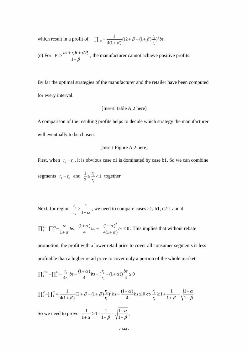
- 144 -
which result in a profit of 21 ((2 (1 ) )4(1 )
om
s
r bsr
β ββ
= + − ++
∏ .
(e) For 1
s sr
bs r R PP ββ
+ +≥
+, the manufacturer cannot achieve positive profits.
By far the optimal strategies of the manufacturer and the retailer have been computed
for every interval.
[Insert Table A.2 here]
A comparison of the resulting profits helps to decide which strategy the manufacturer
will eventually to be chosen.
[Insert Figure A.2 here]
First, when o sr r= , it is obvious case c1 is dominated by case b1. So we can combine
segments o sr r= and 1 12
o
s
rr
≤ < together.
Next, for region 11
o
s
rr α≥
+, we need to compare cases a1, b1, c2-1 and d.
21 1 (1 ) (1 ) 0
1 4 4(1 )a bI I bs bs bsα α α
α α+ −
− = − = − ≤+ +
∏ ∏ . This implies that without rebate
promotion, the profit with a lower retail price to cover all consumer segments is less
profitable than a higher retail price to cover only a portion of the whole market.
2 1 1 (1 ) ( (1 )) 04 4 4
c b s sI I
o o
r r bsbs bsr r
α α− +− = − = − + ≤∏ ∏
1 21 (1 ) 1 1(2 (1 ) ) 0 14(1 ) 4 1 1
d b o oI I
s s
r rbs bsr r
α αβ ββ β β
+ +− = + − + − ≤ ⇔ ≥ + −
+ + +∏ ∏
So we need to prove 1 1 111 1 1
αα β β
+≥ + −
+ + +,

- 145 -
Let 1 1( )1
f xx xα α
α+
= − −+
with ( ]1 ,2x α∈ + .
3 2 2
1 1 1 1 1( ) (1 (1 ) ) 0 ( 1 ) ( 1 ) 02 2
f x x f x f xx x xα α β α+′⇒ = − + = − + ≥ ⇒ = + > = + =
Hence, we have proved strategy in case b1 dominates the rest when 1 11
o
s
rrα
≤ <+
.
Next, consider the situation where 1 12 1
o
s
rr α
≤ <+
, we need to compare case a2, c2-1
and d.
22 2 1 (2 )(1 ) 0
4 4a c o s o sI I
s o s o
r r r rbs bsr r r r
− −− = − − = − ≤∏ ∏
2 2
2 2
1(1 ) ((2 (1 ) ) 04(1 )
4(1 )(1 ) (2 (1 ) ) 0 ( (1 ) ) 0
a d o oI I
s s
o o o
s s s
r rbs bsr r
r r rr r r
β ββ
β β β β β
− = − − + − + ≤+
⇔ − + − + − + ≤ ⇔ − − + ≤
∏ ∏
2 1 21 ((2 (1 ) )4 4(1 )
c d s oI I
o s
r rbs bsr r
β ββ
− − = − + − ++
∏ ∏

- 146 -
It is easy to verify that 11 01
c doI I
s
rr β= ⇒ − =
+∏ ∏ , 211 0
2c doI I
s
rr= ⇒ − ≤∏ ∏ , and
2 11 0c doI I
s
rr
−= ⇒ − ≥∏ ∏ . So if 1 12 1
o
s
rr β
≤ ≤+
, the manufacturer chooses case d;
otherwise if 1 11 1
o
s
rrβ α
< <+ +
, he chooses case c2-1.
Last, for the situation where 11 2
o
s
rr
ββ< <
+, case d dominates case a2.

- 147 -
Proof of Lemma 4.1:
Taking the derivatives with respect to Q, R , and e , respectively, we get
( ) ( ) ( )Io o s
Qp r R c p r R F ar RQ e
∂= − − − − −
∂∏
0( ) ( ) ( )s
Q ar RI eo o s o s
Qr Q r e F y dy ar e p r R F ar RR e
−∂= − + + − −
∂∏ ∫
Because I
Q∂∂∏ strictly decreases with Q and I
R∂∂∏ strictly decreases with R ,
IΠ is strictly concave in both Q and R .
20
0
( ) ( ) ( ) ( ) ( )
( ) ( ) ( ) ( )
s
s
Q ar RI eo s
Q ar Re
o s
Q Qp r R F y dy e F ar R V ee e e e
Q Qp r R F ar R F y dy V ee e e
−
−
∂ ∂⎛ ⎞= − − + ⋅ − ⋅ − −⎜ ⎟∂ ∂⎝ ⎠∂⎛ ⎞= − − − −⎜ ⎟ ∂⎝ ⎠
∏ ∫
∫
2 2 2
2 3 2( ) ( ) ( )Io s
Q Qp r R f ar R V ee e e e
∂ ∂⇒ = − − − −
∂ ∂∏
Because ( )V e is convex in e , so IΠ is also strictly concave in e .

- 148 -
Proof of Theorem 4.4:
With the optimal choices of the retailer, the manufacturer’s profit function follows as
( )( , ) ( ) ( , ) ( ) ( , ) ( , )b b b bm o o sw R w c r R Q w R w c r R ar R Q w R e w R= − − = − − + ⋅∏ ,
where ( , )
( , ) 0( ) | ( ) ( ) ( )
b
b
Q w Rs oe e w R
V e a p w r R p r R ydF ye =
∂= − + −
∂ ∫ ,
11 1( , )1
0
1( , ) ( ) ( ) ( )b kQ w Rb k
s oe w R b a p w r R p r R ydF yk
−− ⎧ ⎫⇒ = − + −⎨ ⎬⎩ ⎭
∫
which imply the manufacturer’s functions can always be written as a form of
11
1( , ) ( , )b km w R Z w R b −Π = ⋅ . So the manufacturer’s optimal choices ( , )b bw R are not
affected by the value of b . The retailer’s profit function is uniquely determined by
the promotional effort level, hence,
( , )
1( , )10
1 1( , )10
( ( , ), ( , )) ( , ) ( ) | ( ( , ))
1( 1) ( ) ( ) ( )
1( 1) ( ) ( ) ( )
b b b
b b b
b b b
b b b b b b b b b b b b br e e w R
kk kQ w Rb b bk
s o
kkQ w Rb bk
s o
Q w R e w R e w R V e V e w Re
b k b a p w r R p r R ydF yk
b k a p w r R p r R ydF yk
=
−−
−−
∂Π = −
∂
⎧ ⎫= − − + −⎨ ⎬⎩ ⎭
⎧ ⎫= ⋅ − − + −⎨ ⎬⎩ ⎭
∫
∫
So the retailer’s profit can be written as a form of 1
12( , ) ( , )b b b b b k
r w R Z w R b −Π = ⋅ .
Similarly, the integrated channel profit can also be represented by
11
3( ) ( )I I kI R Z R b −Π = ⋅ . Therefore, 1 2
3
( , ) ( , )( )
b b b b b bm r
II
Z w R Z w RZ R
Π +Π +=
Π.

- 149 -
Proof of Lemma 4.2:
First we prove it by contradiction. For any given R , we assume ( ( ), ) ( )b b IQ w R R Q R≥ .
Because ( , )br Q e e∂ ∂∏ has the exact form of ( , , )I Q e R e∂ ∂∏ as follows
0( , ) ( ) ( ) ( ) ( )s
Q ar Re
o sQ QZ Q e p r R F ar R F y dy V ee e e
− ∂⎛ ⎞= − ⋅ − − −⎜ ⎟ ∂⎝ ⎠∫
2
2 2
3 2
( ) ( )0
( ) ( ) ( )
o s
o s
Q Qp r R f ar Re Z Q e eQ Z e Q Qp r R f ar R V e
e e e
− −∂ ∂ ∂⇒ = − = − >
∂ ∂ ∂ ⎧ ⎫∂− − ⋅ − +⎨ ⎬∂⎩ ⎭
.
Hence, we can get ( , ) ( )b Ie w R e R≥ . Since ( )V e is convex, so
( , ) ( )
( ) ( )b Ie e w R e e R
V e V ee e= =
∂ ∂≥
∂ ∂. And, the first order condition of optimal promotional
effort can be denoted by ( )0( ) ( ) ( ) ( ) ( ) ( )Q
o sV e p r R ar R Q F Q F y dy Z Qe∂
= − + ⋅ − =∂ ∫ . It is
easy to show that ( )Z Q is strictly increasing with the variable Q . Hence, we should
have ( ( ), ) ( )b b IQ w R R Q R≥ . However,
1 1( )( ( ), ) ( ) ( ) ( )b
b b Io
o o
p r R cp w RQ w R R F F Q Rp r R p r R
− − − −−= < =
− −. Thus, we prove
( ( ), ) ( )b b IQ w R R Q R< .
Alternatively, ( ( ), ) ( )b b IQ w R R Q R< may be proved as follows by taking
( ( ), ) ( )b br Iw R R RΠ <Π for granted. For any given R , we have
( ( ), )( ( ( ), ), ( ( ), )) ( ( ), ) ( ) | ( ( ( ), ))b b
b b b b b b b b br e e w R R
Q w R R e w R R e w R R V e V e w R Re =
∂Π = −
∂
( )( , , ( )) ( ) ( ) | ( ( ))I
I I I II e e R
Q R e R e R V e V e Re =
∂Π = −
∂
Because of ( ( ), ) ( )b br Iw R R RΠ <Π , from the proof in theorem 4.2., we can get
( ( ), ) ( )b b Ie w R R e R< . Hence, for any ( )bow R r R c> + , the following condition holds
( ) ( )( ( ), ) ( ( ), ) ( ( ), ) ( ) ( ) ( )b b b b b I Is sQ w R R ar R Q w R R e w R R ar R Q R e R Q R= + < + = .

- 150 -
Proof of Theorem 4.5:
First we prove that ( , , )IS Q R eQ
is strictly decreasing in .Q
2 0
0
2
( , , ) 1( ) ( ) 0
( ) ( )
1 1( ) ( ) ( )
s
s
I Q ar R se
Q ar Rse
s s s
Q ar RS Q R e e F y dy FQ Q Q Q e
Q ar RQF y dy Fe e
Q ar R Q ar R Q ar RQF F fe e e e e e
−
−
⎛ ⎞ −∂= − <⎜ ⎟∂ ⎝ ⎠
−⇔ <
− − −⇔ < +
∫
∫
So ( , )w Q R is indeed a quantity discount schedule for any 2 0k ≥ .
With quantity discount and buy-back contract, the retailer’s profit function is
( )( )1 2
( , ) ( , ) ( , , ) ( ) ( , , ) ( )
( ) ( , , ) ( ) ( ) ( , , )r
Io o
Q e w Q R Q pS Q R e b R Q S Q R e V e
cQ p r R S Q R e V e k cQ p r R S Q R e k
= − + + − −
= − + − − − − + − −
∏
Take the first derivative with respect to e , we have
( , ) ( , , ) ( )( ) 0ro
Q e S Q R e V ep r Re e e
∂ ∂ ∂= − − =
∂ ∂ ∂∏
Hence, the retailer chooses the optimal effort level Ie . With the chosen optimal effort
level,
1( , ) ( , , )(1 ) ( )
I Ir
oQ e S Q R ek c p r RQ Q
⎛ ⎞∂ ∂= − − + −⎜ ⎟∂ ∂⎝ ⎠
∏ .
Hence, the retailer also chooses the optimal order quantity IQ .
Apparently, with the anticipation of the retailers choices, the manufacturer’ profit
function is
( )1 1 2
1 2 1
( ) ( ( , ) ) ( , , ) ( ) ( , , )
( ) ( , , )
( , , ) ( )
I I I I I I Im o
I I Io
I I II
R w Q R c Q r RS Q R e b R Q S Q R e
k cQ k p r R S Q R e k
k Q R e k k V e
= − − − −
= − + − +
= + +
∏
∏
Hence, the manufacturer’s decision on rebate value is IR .

- 151 -
Proof of Theorem 4.6:
At the undiscounted price level 1w , similar to lemma 4.2, we can obtain the optimal
order quantity for the retailer satisfies the condition 1 1 1( , ) ( )b IQ w R Q R< . Obviously,
the manufacturer can always find a 1R such that 1( )I IQ R Q≤ , for example, simply by
choosing 1IR R= .
At the discounted price level 2w , the retailer chooses IQ as his optimal order
quantity. Because
2
2 2 0
( , ) ( ) ( ) ( ) ( ) 0I
sI I I Q ar Rr e
o sQ e Q Qp r R F ar R F y dy V ee e e e
−⎛ ⎞∂ ∂= − ⋅ − − − =⎜ ⎟∂ ∂⎝ ⎠
∏∫ (4.9)
So for any given rebate value 2R , the retailer’s promotional decision is not distorted
and not related to 2w , denote by 2( )de R , which can be solved from (4.9).
Hence, the manufacturer’s problem is to maximize the following profit function,
2 2 2 2( , ) ( ) Im ow R w r R c QΠ = − − ,
with the constraint that
2( )2 2 2 2 1 10
( ) ( ) ( ) ( ) ( ( )) (1 ) ( , )dQ RI d d b
r o rp w Q p r R e R F y dy V e R w RλΠ = − − − − ≥ + Π∫
where 2 22
( )( )
Id
d s
QQ R ar R
e R= −
Hence, ( )2( )2 1 1 2 2 20
1 (1 ) ( , ) ( ) ( ) ( ) ( ( ))dQ Rb d d
r oIw p w R p r R e R F y dy V e RQ
λ≤ − + Π + − +∫ ,
or 2
2 1 1 2 2 2 2( )
1 (1 ) ( , ) ( ) ( ( )) ( ) ( ) | ( ( ))db I d d dr oI e e R
w p w R p r R Q F Q R e R V e V e RQ e
λ=
∂⎛ ⎞≤ − + Π + − − +⎜ ⎟∂⎝ ⎠.
So the manufacturer’s problem is equivalent to maximize
( ){ }2( )2 2 2 2 1 10
( ) ( ) ( ) ( ) ( ) ( ) (1 ) ( , )dQ RI d d b
m o o rR p r R c Q p r R e R F y dy V e R w RλΠ = − − − − − − + Π∫ .
The first term of the above function is in exactly the same form as the integrated
channel. So the manufacturer will announce 2IR R= . As long as the manufacturer

- 152 -
choose the optimal IR , the retailer’s promotional effort will be adjusted accordingly
to the level Ie since the retailer’s promotional decision is not distorted. With these
optimal choices, the manufacturer’s wholesale price is
2 1 1
1 1
1 ( ) ( ) | ( ) (1 ) ( , )
(1 ) ( , )
II I I I b
o rI e e
bI I r
o I
w r R c Q e V e V e w RQ e
w Rr R cQ
λ
λ
=
∂⎛ ⎞= + + − − + Π⎜ ⎟∂⎝ ⎠Π − + Π
= + +
and his maximum profit is denoted by 1 1(1 ) ( , )d bm I r w RλΠ =Π − + Π .
However, the discounted wholesale price should be less than the undiscounted one,
i.e., 2 1w w< . Hence,
( ){ }
2
2
( )2 1 1 2 2 2 10
( )1 2 2 20
1 1
1 (1 ) ( , ) ( ) ( ) ( ) ( ( ))
1 ( ) ( ) ( ) ( ) ( ( )) 1( , )
d
d
Q Rb d dr oI
Q RI d dob
r
w p w R p r R e R F y dy V e R wQ
p w Q p r R e R F y dy V e Rw R
λ
λ
= − + Π + − + <
⇔ > − − − − −Π
∫
∫
Given if the manufacturer chooses a 1w sufficiently close to the retail price p , the
above condition can always be satisfied.

- 153 -
Figure A.1. The Manufacturer’s Candidate Strategy Sets in Decentralized Channel
Figure A.2. The Manufacturer’s Candidate Strategy Sets in Integrated Channel

- 154 -
a2 b1 c1 c2 d1 d2
Con
ditio
n
1o
s
rr
αα
≤+
1
1o
s
rr α≥
+1o
s
rr= 1o
s
rr<
1o
s
rr
ββ
>+
1
o
s
rr
ββ
≤+
w
1bsα
α+
2bs
2bs
2(1 )2( (1 ) )
s o
s o
r r bsr r
ββ
+ ++ +
bs 2( )
2 2 2o
s
r bsr
ββ
++
+
R
s
bsr
0 0 1
2( (1 ) )s o
bsr r
ββ
++ +
(1 )
(1 )s o
bsr r
ββ
++ +
s
bsr
sP bs bs (3 )
4 2bsββ
++
bs bs bs
rP bs 3
4bs
(3 )4 2
bsββ
++
bs 3 2(1 )2( (1 ) )
s o
s o
r r bsr r
ββ
+ ++ +
3(2 )( )4(1 ) 4
o
s
r bsr
ββ
++
+
D 1 14α+
14 2
ββ
++
(1 )2( (1 ) )
s
s o
rr r
ββ
++ +
(1 )
2( (1 ) )s
s o
rr r
ββ
++ +
1 (2 (1 ) )4
o
s
rr
β β+ − + ⋅
rΠ 11
bsα+
1
16bsα+
2
14(2 )
bsββ
++
2
2
(1 )4( (1 ) )
s
s o
r bsr r
ββ
++ +
2
2
(1 )4( (1 ) )
s
s o
r bsr r
ββ
++ +
21 (2 (1 ) )16(1 )
o
s
r bsr
β ββ
+ − ++
mΠ ( )1
o
s
r bsr
αα−
+ 1
8bsα+
14(2 )
bsββ
++
(1 )
4( (1 ) )s
s o
r bsr r
ββ
++ +
2
2
(1 )2( (1 ) )
s
s o
r bsr r
ββ
++ +
21 (2 (1 ) )8(1 )
o
s
r bsr
β ββ
+ − ++
r mΠ +Π (1 )o
s
r bsr
− 3(1 )
16bsα+ 2
(1 )(3 )4(2 )
bsβ ββ
+ ++
2
(1 ) (2 (1 ) )4( (1 ) )
s s o
s o
r r r bsr r
β ββ
+ + ++ +
2
2
3(1 )4( (1 ) )
s
s o
r bsr r
ββ
++ +
23 (2 (1 ) )16(1 )
o
s
r bsr
β ββ
+ − ++
Table A.1. The Candidate Solution Sets in Decentralized Channel
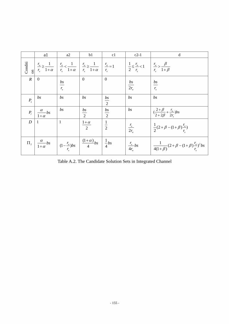
- 155 -
a1 a2 b1 c1 c2-1 d
Con
diti
on
11
o
s
rr α≥
+
11
o
s
rr α<
+
11
o
s
rr α≥
+1o
s
rr=
1 12
o
s
rr
≤ < 1
o
s
rr
ββ
>+
R 0
s
bsr
0 0
2 o
bsr
s
bsr
sP bs bs bs
2bs
bs bs
rP 1
bsαα+
bs
2bs
2bs
bs 2( )
2 2 2o
s
r bsr
ββ
++
+
D 1 1 12α+
12
2
s
o
rr
1 (2 (1 ) )2
o
s
rr
β β+ − +
IΠ 1
bsαα+
(1 )o
s
r bsr
− (1 )
4bsα+ 1
4bs
4s
o
r bsr
21 (2 (1 ) )4(1 )
o
s
r bsr
β ββ
+ − ++
Table A.2. The Candidate Solution Sets in Integrated Channel

- 156 -
LIST OF REFERENCES
- 157 -
Arcelus, F.J., Kumar, S. and Srinivasan, G. (2006). “Retailer’s response to alternate manufacturer’s incentives under a single-period, price-dependent, stochastic-demand framework”, Decision Sciences, 36(4)
Ault, W.R., R. Beard, D.N. Laband and R.P. Saba (2000) “Rebates, inventories, and
intertemporal price discrimination”, Economic Inquiry, 38(4) 570-578. Aydin, G. and E.L. Porteus (2005) “The Effects of Retailer versus Consumer Rebates
in a Supply Chain”, Working Paper, The University of Michigan Balasubramanian, S. and P. Bhardwaj (2004) "Manufacturing-Marketing Conflict and
Strategic Incentive Design” Management Science, 50(4), 489–502 Baysar, O., O.C. Demirag, P. Keskinocak and J.L. Swann (2006) “The effects of
customer rebates and retailer incentives on manufacturer profitability and sales”, Manuscript submitted to Management Science.
Bell, D.R. and J.M. Lattin (2000) "Looking for Loss Aversion in Scanner Panel Data:
The Confounding Effect of Price Response Heterogeneity", Marketing Science, 19(2), 185–200
Bell, D.R., Y. Wang and V. Padmanabhan (2003) “The effect of partial forward
integration on retailer behavior: an explanation for co-located stores”, Working Paper, University of Pennsylvania
Blattberg, R.C. and S.A. Neslin (1990), “Sales Promotion: Concepts, Methods and
Strategies”, Englewood Cliffs, NJ: Prentice Hall. Blattberg, R.C. and K.J. Wisniewski (l989), "Price-Induced Patterns of Competition,”
Marketing Science 8 (4), 291-309. Blattberg, R.C. and S.A. Neslin(1990), “Sales Promotion: Concepts, Methods and
Strategies”, Englewood Cliffs, NJ: Prentice Hall. Blattberg, R.C., R. Briesch and E.J. Fox (1995). “How promotions work”, Marketing
Science 14(3-2) Bulkeley, W.M. (1998), “Rebates' Secret Appeal to Manufacturers: Few Consumers
Actually Redeem Them”, Wall Street Journal (Eastern edition), New York, pg. B.1
Cachon, G.P. (2003) “Supply chain coordination with contracts”, Chapter in
Handbooks in Operations Research and Management Science: Supply Chain Management. Graves, S. and Kok, T.de, eds. North-Holland.

- 158 -
Cachon, G.P. (2004) “The Allocation of Inventory Risk in a Supply Chain: Push, Pull,
and Advance-Purchase Discount Contracts”, Management Science 50(2), 222-238
Cachon, G.P. (2006), “You say ‘channels’, I say ‘supply chains’: Shall we get it on, or
call the whole thing off?”, Working paper, University of Pennsylvania. Cachon, G. P. and M. A. Lariviere (2005) “Supply chain coordination with
revenue-sharing contracts: strengths and limitations”, Management Science 51(1), 30-44.
Chan, L.M.A., Z.J.M. Shen, D. Simchi-Levi and J.L. Swann (2003) “Coordination of
pricing and inventory decisions: a survey and classification”, Chapter in Handbook of Quantitative Supply chain analysis in the eBusiness era. Simchi-Levi, D., Wu, S.D. and Shen, Z-J., eds. Kluwer Academics Publishers.
Chen, F., F. Awi and Y. Zheng (2001) "Coordination Mechanisms for a Distribution
System with One Supplier and Multiple Retailers" Management Science 47(5), 693–708
Chen, X., C.-L. Li and D. Simchi-Levi (2005) “The impact of manufacturer rebates
on supply chain profits”, Working Paper, University of Illinois at Urbana-Champaign.
Chen, Y., S. Moorthy and Z.J. Zhang (2005), “Price discrimination after the purchase:
Rebates as state-dependent discounts”, Management Science 51, 1131-1140. Cheng, F. and S.P. Sethi (1999) “A periodic review inventory model with demand
influenced by promotion decisions”, Management Science, 45(11), 1510-1523 Choi, S.C (2003) "Quantity Discounts for Channel Coordination: Transaction and
Channel Efficiency", Working Paper, Rutgers University Choi, C., L. Lei and Q. Wang (2003) “Quantity Discounts for Supply chain
Coordination”, Chapter in Managing Business Interfaces: Marketing, Engineering, and Manufacturing Perspectives. Chakravarty, A.K. and Eliashberg, J., eds. Kluwer Academics Publishers.
Chu, W. and P. S. Desai (1995) “Channel coordination mechanisms for customer
satisfaction”, Marketing Science 14(4) 343–359. David R.B. and J.M. Lattin (1998) "Shopping Behavior and Consumer Preference for
Store Price Format: Why "Large Basket" Shoppers Prefer EDLP" Marketing

- 159 -
Science 17(1), 66-88. Desai, P.S. and P. Padmanabhan (2004) “Durable Good, Extended Warranty and
Channel Coordination”, Review of Marketing Science, 2(2) Dogan, K., E. Haruvy and R.C. Rao (2005) "Segmentation and Competition: An
Application to Rebates", working paper, University of Texas at Dallas Dreze, X. and D.R. Bell (2003) “Creating Win–Win Trade Promotions: Theory and
Empirical Analysis of Scan-Back Trade Deals”, Marketing Science, Vol.22, No.1, 16-19
Eliashberg, J. and R. Steinberg (1987) “Marketing-production decisions in an
industrial channel of distribution”, Management Science, 33(8), 981-1000. Erdem, T., G. Mayhew and B. Sun (2001) “Understanding reference-price shoppers: A
within- and cross-category analysis”, Journal of Marketing Research, 38(4) Folkes, V. and R.D. Wheat (1995) “Consumers price perceptions of promoted
products”, Journal of Retailing 71 (3), 317–328. Gerstner, E. and J. Hess (1991) “A Theory of Channel Price Promotions,” The
American Economic Review, 81(4), 872-886 Gerstner, E., J. Hess and D. Holthausen (1994) “Price discrimination through a
distribution channel: theory and evidence,” The American Economic Review, 84(5), 1437-1445
Gerstner, E. and J. Hess (1995) “Pull promotions and channel coordination”,
Marketing Science, 14(1), 43-60 Gilpatric, S.M. (2005) “A Behavioral Theory of Rebates: Present-Biased Preferences
and Redemption”, working paper, University of Tennesse Gourville, J.T. and D. Soman (2004) “The consumer psychology of mail-in rebates: a
model of anchoring and adjustment”, working paper, Harvard Business School. Greenleaf, E.A. (1995), "The Impact of Reference Price Effects on the Profitability of
Price Promotions", Marketing Science 14 (1), 82-104. Grow, B. (2005), “The Great Rebate Runaround”, Business Week, Nov.23 Gurnani, H. and Y. Xu, (2006) “Resale Price Maintenance contracts with retailer sales
effort: Effect of Flexibility and competition”, Naval Research Logistics, 10.1002

- 160 -
Hardie, B., E.J. Johnson and P.S. Fader (1993) “Modeling loss aversion and reference
dependence effects on brand choices”, Marketing Science, 12(4), 378-394 Hess, J.D. and M.T. Lucas (2004) “Doing the Right Thing or Doing the Thing Right:
allocating resources between marketing research and manufacturing”, Management Science, 50(4)
Ho, T., C.S. Tang and D.R. Bell (1998) "Rational Shopping Behavior and the Option
Value of Variable Pricing", Management Science 44(12), Part 2 of 2, S145-S160. Hoch, S.J., X. Dreze and M.E. Purk (1994) "EDLP, Hi-Lo, and Margin Arithmetic",
Journal of Marketing 58(4), 16-27 Huang, Z., S.X. Li and V. Mahajan (2002) “An analysis of manufacturer–retailer
supply chain coordination in cooperative advertising”, Decision Sciences 33, 469–494.
Inman, J. J., L. McAlister and W.D. Hoyer (1990) “Promotion signal: proxy for a
price cut?”, Journal of Consumer Research, 17 (June), 74-81. Iyer, G. and V. Padmanabhan (2003) “Contractual relationships and coordination in
distribution channels”, Chapter in Managing Business Interfaces: Marketing, Engineering, and Manufacturing Perspectives. Chakravarty, A.K. and Eliashberg, J., eds. Kluwer Academics Publishers.
Jeuland A.P. and S.M. Shugan (1983) “Managing Channel Profits”, Marketing
Science, 2(3) Jolson, M.A., J.L. Wiener and R. Rosecky (1987). “Correlates of rebate proneness”.
Journal of Advertising Research 27 (1), 33–44. Joseph, K. and J. Lemieux (2005) “The Optimal Design of Rebate Programs”,
working paper, University of Kansas. Kalyanaram, G. and R.S. Winer (1995) "Empirical Generalization from Reference
Price Research", Marketing Science, 14(3-2) Khouja, M. (2003) “Joint pricing and delayed incentive model for maximizing
profits”, Working paper, the University of North Carolina at Charlotte, Charlotte, NC, 28223.
Khouja, M. (2006) “A Joint optimal pricing, rebate value, and lot sizing model for
maximizing profits”, European Journal of Operational Research 174, 706-723

- 161 -
Krishnan, H., R. Kapuscinski and D.A. Butz (2004) “Coordinating contracts for
decentralized supply chain with retailer promotional effort”, Management Science 50(1), 48-63
Kuman, N., S. Rajiv, and A. Jeuland (2001) “Effectiveness of Trade Promotions:
Analyzing the Determinants of Pass Through”, Marketing Science, Vol20, No.4 382-404
Lal, R. (1990) “Improving channel coordination through franchising”, Marketing
Science, 9(4) Lal, R., D.C. Little and J.M. Villas-Boas (1996) “A Theory of Forward Buying,
Merchandising, and Trade Deals”, Marketing Science,15(1) Lal, R. and R. Rao (1997)"Supermarket Competition: The Case of Every Day Low
Pricing", Marketing Science 16(1), 60-80 Lattin, J.M. and G. Ortmeyer (1991) "A theoretical rationale for everyday low pricing
by grocery retailers”, Research Paper No. 1144. Graduate School of Business, Stanford University
Lee, E. and R. Staelin (1997) Vertical strategic integration: implications for channel
pricing strategy, Marketing Science, 16(3), 185-207 Li, S.X., Z. Huang, J. Zhu and P.Y.K. Chau (2002) “Cooperative advertising, game
theory and manufacturer–retailer supply chains”, Omega, 30, 347–357 Lieber, D. (2005) “Rebate = Hassle: State, federal regulators begin to take a closer
look”, Dave Lieber's Watchdog column on Star-Telegram News Lim, N and T. Ho (2006) “Designing Price Contracts for Boundedly Rational
Customers: Does the Number of Blocks Matter?”, Forthcoming in Marketing Science
Mayhew, G.E. and R.S. Winer (1992) "An Empirical Analysis of Internal and External
Reference Prices Using Scanner Data", The Journal of Consumer Research, 19(1), 62-70.
Mitchell, R.L. (2005), “High-tech retailers, low-tech rebates”, Computerworld Daily
News Moorthy, K.S. (1988), “Product and Price Competition in a Duopoly,” Marketing
Science 7 (2), 141-168.

- 162 -
Moorthy, K.S. and D. Soman (2003) “ On the marketing of rebates: Having your cake
and eating it too?”, Working paper, University of Toronto Moorthy, K.S. and Q. Lu (2004) “Coupons versus Rebates”, working paper,
University of Toronto. Munson, C.L. and M.J. Rosenblatt (1998) "Theories and Realities of Quality
Discounts: An Exploratory Study", Production and Operations Management 7(4), 352-369
Neslin, S.A. (2002), “Sales Promotion”, Chapter in Handbook of Marketing. Weitz, B.
and Wensley, R., eds. Sage Publications. Neslin, S.A., C. Henderson and J. Quelch (1985) “Consumer promotions and the
acceleration of product purchases”, Marketing Science 4(2), Neslin, S.A., S.G. Powell and L.S. Stone (1995), “The effects of retailer and consumer
response on optimal manufacturer advertising and trade promotion strategies”, Management Science 41(5)
Netessine, S. and N. Rudi (2000) “Supply chain structures on the Internet and the role
of marketing-operations interactions”, Chapter in Handbook of Quantitative Supply chain analysis in the eBusiness era. Simchi-Levi, D., Wu, S.D. and Shen, Z-J., eds. Kluwer Academics Publishers.
Novemsky, N. and D. Kahneman (2005) "The Boundaries of Loss Aversion", Journal
of Marketing Research", V. XLII, 119–128 Spencer, J. (2002) “As Cash-Back Offers Multiply, So Do Obstacles for Consumers”,
Wall Street Journal, June 11. Pekgun, P., P. Griffin and P. Keskinocak (2005) “Coordination of Marketing and
Production for Price and Leadtime Decisions”, working paper, Georgia Institute of Technology
Porteus E.L. and S. Whang (1991) “On manufacturing/marketing incentives”,
Management Science, 37(9) Ray, S., S. Li, and Y. Song (2005), “Tailored Supply Chain Decision Making Under
Price-Sensitive Stochastic Demand and Delivery Uncertainty”, Management Science, 51(12), 1873-1891
Rhee, Byong-Duk (1996), “Consumer Heterogeneity and Strategic Quality
- 163 -
Decisions,” Management Science 42(2), 157-172. Rosenkranz, S. (2003), “The Manufacturer’s Suggested Retail Price”, Discussion
Paper Series 03-05, Utrecht School of Economics Silk, T.G. (2004) “Why do we buy but fail to redeem? Examining the breakage of
mail-in rebates”, Doctoral Dissertation, University of Florida. Silk, T. and C. Janiszeweki (2004) “managing mail-in rebate”, working paper,
University of South Carolina. Sogomonian, A.G. and C.S. Tang (1993) “A Modeling Framework for Coordinating
Promotion and Production Decisions within a Firm”, Management Science, 39(2)
Soman, D. (1998) “The Illusion of Delayed Incentives: Evaluating Future
Effort-Money Transactions,” Journal of Marketing Research, 35 (4), 427-437 Spengler, J. (1950) “Vertical Integration and Antitrust Policy”, Journal of Political
Economy, 58(4) 347-352 Tat, P., W.A. Cunningham and E. Babakus (1988) “Consumer perceptions of rebates”,
Jouarnal of Advertising Research, 28(August/September. Taylor, T.A. (2002) “Supply Chain Coordination Under Channel Rebates with Sales
Effort Effects”, Management Science 48(8), 992-1007 Thompson, P. and T. Noordewier (1992) “Estimating the effects of consumer
incentive programs on domestic automobile sales”, Journal of Business and Economic Statistics, 10(10).
Tversky, A. and D. Kahneman (1991) "Loss Aversion in Riskless Choice: A
Reference-Dependent Model", The Quarterly Journal of Economics, 106(4), 1039-1061.
Ulanoff, M. S. (1985) “What is Sales Promotion?”, Chapter in Handbook of Sales
Promotion. Ulanoff, M. S., eds. McGraw-Hill, Inc. Viswanathan, S. and Q. Wang (2003) "Discount pricing decisions in distribution
channels with price-sensitive demand", European Journal of Operational Research 149, 571–587
Wang, Q. and Z. Wu (2000) "Improving a supplier’s quantity discount gain from
many different buyers" IIE Transactions 32, 1071–1079

- 164 -
Wang, Y. and Y. Gerchak (2001) “Supply chain coordination when demand is
shelf-space dependent”, Manufacturing and Service Operations Management, 3(1). 82-87.
Weng, Z.K. (1995) "Channel Coordination and Quantity Discounts", Management
Science 41(9), 1509-1522 Weng, Z.K. (2004) "Coordinating order quantities between the manufacturer and the
buyer: A generalized newsvendor model", European Journal of Operational Research 156, 148–161
Yano, C.A. and S.M. Gilbert (2003) “Coordinated Pricing and
Production/Procurement Decisions: A Review”, Chapter in Managing Business Interfaces: Marketing, Engineering, and Manufacturing Perspectives. Chakravarty, A.K. and Eliashberg, J., eds. Kluwer Academics Publishers.
Yue, J., J. Austin, M.-C. Wang and Z. Huang (2006) “Coordination of cooperative
advertising in a two-level supply chain when manufacturer offers discount”, European Journal of Operational Research, 168, 65-68
Zhang, Z.J., A. Krishna and S. K. Dhar (2000) “The optimal choice of promotional
vehicles: front-loaded or rear-loaded incentives?”, Management Science, 46(3), 448-362