The Pennsylvania State University
The Graduate School
Harold and Inge Marcus Department of Industrial and Manufacturing Engineering
SUPPLIER SELECTION PROBLEM IN CROSS DOCKING
COLD CHAIN
A Thesis in
Industrial Engineering
by
Mengyi Yu 2015 Mengyi Yu Submitted in Partial Fulfillment of the Requirements for the Degree of
Master of Science
December 2015

The thesis of Mengyi Yu was reviewed and approved* by the following: Vittal Prabhu Professor of Industrial Engineering Thesis Advisor Robert Novack Associate Professor of Supply Chain and Information Systems Janis Terpenny Professor of Industrial Engineering Peter and Angela Dal Pezzo Department Head *Signatures are on file in the Graduate School
ii

ABSTRACT
Cross docking is an integrated warehouse where incoming freights are directly loaded onto
outbound trucks. It has been widely used in the retail industry to reduce supply chain costs.
Every retailer wants to sell relatively high quality products while reduce the operation costs
to the minimum. In recent years, the purchasing function has assumed to take larger
proportion of the contribution to the supply chain, and one of the most important
purchasing functions is the selection of the suppliers. The supplier selection problem could
be solved in two phases. The first phase is to reduce the large amount of candidate suppliers
to a relatively manageable small size. The second phase is to form a multiple criteria
optimization model to allocate order quantities among the shortlisted suppliers. This thesis
examines the strategy of supplier selection in a cross docking cold chain. Buyers usually
do not consider from this perspective, but this method may help them to save extra money.
In the first phase, Borda Count, L∞ Norm, and Analytical Hierarchy Process (AHP) have
been used to reduce the original suppliers. An optimization model has been stated in the
second phase to determine which supplier to choose from the reduced suppliers selected in
the first phase. And the two-phase supplier selection method has been performed in an
example. The sensitivity analysis of the example showed that the order allocation among
the suppliers would not change when we varied the inbound shipment capacity.
iii

Table of Contents
LIST OF FIGURES ....................................................................................... vi
LIST OF TABLES ........................................................................................ vii
ACKNOWLEDGEMENTS ........................................................................... ix
1 Introduction ............................................................................................... 1
1.1 Supplier Selection Problem ............................................................... 1 1.1.1 Sourcing Strategy ........................................................................ 2 1.1.2 Criteria for Selection ................................................................... 2 1.1.3 Pre-Qualification of Suppliers .................................................... 3 1.1.4 Final Selection ............................................................................. 3
1.2 An Overview of Cross Docking......................................................... 3 1.3 An Overview of Cold Chain .............................................................. 5 1.4 Objective and Thesis Outlines ........................................................... 5
2 Literature Review ..................................................................................... 7
2.1 Supplier Selection Problem ............................................................... 7 2.2 Cross Docking .................................................................................... 9 2.3 Cold Chain ....................................................................................... 11 2.4 Cross Docking in Cold Chain .......................................................... 12
3 Methodology ...........................................................................................13
3.1 Definitions ........................................................................................ 13 3.2 First Phase ........................................................................................ 20 3.3 Second Phase ................................................................................... 20
3.3.1 Model ........................................................................................20 3.3.2 Assumptions ..............................................................................21 3.3.3 Indices .......................................................................................22 3.3.4 Parameters .................................................................................22 3.3.5 Decision Variables ....................................................................23 3.3.6 Problem Formulation ................................................................24
iv

4 Example and Discussions .......................................................................28
4.1 First Phase ........................................................................................ 28 4.2 Second Phase ................................................................................... 42 4.3 Sensitivity Analysis ......................................................................... 46
5 Conclusions .............................................................................................47
REFERENCES ..............................................................................................48
Appendix A: LINDO Formulation of the Model ..........................................53
Appendix B: The Solution Reports Obtained from LINDO .........................57
v

LIST OF FIGURES
Figure 1 Supplier Selection Problem .................................................................................. 2
Figure 2 Schematic Representation of a Cross Docking Terminal ..................................... 4
Figure 3 The Supply Chain for the Model ........................................................................ 21
Figure 4 Supplier Selection Criteria ................................................................................. 37
vi

LIST OF TABLES
Table 1 Degree of Importance Scale in AHP.................................................................... 15
Table 2 the Value of RI ..................................................................................................... 16
Table 3 Potential Suppliers for Product 1 ......................................................................... 29
Table 4 Potential Suppliers for Product 2 ......................................................................... 29
Table 5 Potential Suppliers for Product 2 ......................................................................... 31
Table 6 Initial Supplier Data for product 2 ....................................................................... 32
Table 7 Normalized Supplier Data for Product 1 ............................................................. 33
Table 8 Normalized Supplier Data for Product 2 ............................................................. 33
Table 9 Preference Matrix of each Criterion .................................................................... 34
Table 10 Borda Count Rank and Weight of each Criterion .............................................. 34
Table 11 Score and Rank of Suppliers for Product 1........................................................ 35
Table 12 Score and Rank of Suppliers for Product 2........................................................ 36
Table 13 Pairwise Comparison Matrix for Product 1 ....................................................... 37
Table 14 Pairwise Comparison Matrix for Product 2 ....................................................... 37
Table 15 Normalized Matrix for Product 1....................................................................... 38
Table 16 Normalized Matrix for Product 2....................................................................... 38
Table 17 Criterion Weights ............................................................................................... 39
Table 18 Consistency Check for Product 1....................................................................... 40
Table 19 Consistency Check for Product 2....................................................................... 40
Table 20 AHP Rank for Product 1 .................................................................................... 41
Table 21 AHP Rank for Product 2 .................................................................................... 41
vii

Table 22 Notation of Reduced Suppliers .......................................................................... 42
Table 23 Model Summary ................................................................................................ 44
Table 24 Order Allocated to Each Supplier (in Percent) .................................................. 45
Table 25 Order Allocated to Original Supplier Notation (in Percent) .............................. 45
Table 26 Allocation for Different Scenarios ..................................................................... 46
viii

ACKNOWLEDGEMENTS
I am really thankful for my thesis advisor, Professor Prabhu. Without his support, there is
no way that this thesis could progress towards its full completion. His insightful comments,
intellectual guidance and remarkable patience helped me construct original thoughts into
this full-fledged form. And also I would like to express gratitude to my thesis reader
Professor Novack, who reviews my work in the final phase. Finally, special thanks to my
friends, Xuan Li, Maiteng Pornthip and Vara-Urairat Putthipan, and family members who
gave me so much support both academically and emotionally.
ix

1 Introduction
1.1 Supplier Selection Problem
In this highly competitive world, an effective supplier selection process is significant to the
success of retailers. In most cases, buyers from a company need to choose among a set of
suppliers by using some predetermined criteria such as quality, reliability, technical
capability, lead-times, etc. Therefore, two basic and interrelated decisions must be made
by a company before building any long-term relationships with suppliers, as presented in
the following questions:
1. Which suppliers to do business with?
2. How much to order from each supplier?
Weber et al. define this pair of decisions as the supplier selection problem (Weber, et al.,
1991).
The supplier selection problem is considered to be complicated because most of the criteria
for selecting are conflicting. Supplier selection is a multiple criteria optimization problem
that requires the decision maker considering the trade-offs among different qualitative and
quantitative factors (Ravindran & Warsing, 2012).
The supplier selection methods are explicitly discussed in Dr. Ravindran’s book.
(Ravindran & Warsing, 2012)
Figure 1 shows the typical decision making procedures for supplier selection problem.
1

Figure 1 Supplier Selection Problem (Ravindran & Warsing, 2012)
1.1.1 Sourcing Strategy
Depending on the type of items being purchased, the sourcing strategy could be either
strategic or tactical. When the item being purchased is expensive and critical, and can only
be bought from certain suppliers, the sourcing strategy tends to be more strategic; when
the item could be easily purchased from several suppliers in the market, the supplier
selection is a tactical decision.
1.1.2 Criteria for Selection
Criteria for supplier selection have been studied since the 1960s. Pal et al. thoroughly
reviewed present paper regarding to the supplier selection criteria and methods in supply
chains and concluded that price, delivery, and quality are considered to be the top three
most important criteria for supplier selection (Pal, et al., 2013).
2

1.1.3 Pre-Qualification of Suppliers
Pre-qualification is defined as the process of reducing a large set of potential suppliers to a
smaller manageable number by ranking the suppliers under a pre-defined set of criteria.
(Holt, 1998) The benefits of pre-qualification of suppliers are presented as following:
1. The possibility of rejecting good suppliers at an early stage is reduced.
2. Resource commitment of the buyer toward purchasing process is optimized.
3. With the application of pre-selected criteria, the pre-qualification process is rationalized.
1.1.4 Final Selection
In this step, the purchaser decides which suppliers to do business with and allocates order
quantities among the chosen suppliers. As proposed by Ghodsypour & O’Brien, there are
two types of basic supplier selection problem (Ghodsypour & O'Brien, 2001):
1. Single Sourcing, which supposes that each one of the suppliers could satisfy the buyer’s
requirements of demand, quality, delivery, etc.
2. Multiple Sourcing, which considers that there are certain limitations in suppliers’
capacity, quality, etc. so that multiple suppliers have to be used.
1.2 An Overview of Cross Docking
Cross docking is a “process of consolidating freight with the same destination (but coming
from several origins), with minimal handling and with little or no storage between
unloading and loading of the goods” (Belle, et al., 2012). Cross docking has been widely
used by many companies such as Wal-Mart (United States), Carrefour (France), Albert
Heijn (the Netherlands), and Tesco (United Kingdom). Implementation of proper cross
3

docking has many advantages compared to traditional warehouses such as reduction or
even elimination of merchandise storage, and order-picking. Thus the inventory holding
cost and labor cost would be reduced (Galbreth, et al., 2008).
Figure 2 shows a schematic representation of a cross docking terminal (Stephan & Boysen,
2011). At the inbound doors, trucks are unloaded and shipments are registered. The
shipments will be checked for completeness and intactness, and be sorted according to their
destinations. Then shipments will be moved across the dock to their temporary storage area
which has been assigned by the intended destination of the shipments. In the meantime,
value adding services would be performed such as labeling while the shipments are waiting
for the outbound truck. Lastly, shipments will be loaded onto outbound trucks to leave the
terminal for their next destinations.
Figure 2 Schematic Representation of a Cross Docking Terminal (Stephan & Boysen, 2011)
4
1.3 An Overview of Cold Chain
A cold chain protects a large variety of products from deterioration such as food,
pharmaceutical and chemical products. It insulates them from degradation, improper
exposure to temperature, humidity, light or particular contaminants, and keeps them frozen,
chilled and fresh (Bishara, 2006). The typical cold chain infrastructure contains pre-cooling
facilities, cold storages, refrigerated carriers, packaging, warehouse, traceability, retailer,
and customers. And these facilities are under control of the information management
systems (Montanari, 2008). However, Manikas & Terry stated that the efficiency of the
food cold chain is not high enough even though automatic machines have been applied to
this industry. Large parts of this logistic process is still handled manually such as picking
process since it is hard to control the process by machines (Manikas & Terry, 2009).
1.4 Objective and Thesis Outlines
Many retailers have a large amount of suppliers to choose from. This thesis extended a
two-phase supplier selection strategy in a cross docking cold chain. The main objective of
supplier selection for retailers is to reduce purchase risk, to maximize overall value, and to
develop long-term relationship with suppliers in this competitive industrial world. The
supplier selection problem, cross docking arrangement and cold supply chain have been
studied by many researchers. However, very few studies address the perspective: supplier
selection in cross docking cold chain. This thesis aims to fill this gap of researches.
The next chapter provides the literature review on studies of supplier selection problem,
cross docking operation and cold chain management. Chapter 3 discussed the two-phase
supplier selection method in the cross docking cold chain. Borda Count, L∞ Norm, and
5

AHP have been used in the first phase to reduce the original suppliers. Then an optimization
model of supplier selection problem in cross docking cold chain is presented in the second
phase, to make final selection of suppliers. Parameters and decision variables used in the
optimization model are discussed; assumptions for mathematical formulation of the model
are made. The solution to this optimization model is computationally intractable when the
problem size grows even modestly. Thereafter, the model is implemented to an example
using the modeling tool LINDO and the results are analyzed. The thesis ends with
conclusion of the final remarks.
6

2 Literature Review
2.1 Supplier Selection Problem
An Analytical Hierarchy Process (AHP)-based model was formulated and implemented to
a real case study by Tam & Tummala to examine its feasibility in selecting suppliers for a
telecommunication system. The results showed that using the proposed model, the group
decision making in selecting vendors, which can satisfy customer demands, was improved.
The time consuming pairwise comparison judgements could be avoided by applying the
suggested five-point rating system (Tam & Tummala, 2001).
Humphreys et al. developed a framework for integrating environmental factors into the
supplier selection process. For example, quality and flexibility are traditional factors that
companies would consider for evaluating supplier performance. However, many
companies start to consider environmental criteria and measure their suppliers’
environmental performance to accommodate the increase of the environmental pressure. A
knowledge-based system was constructed and could guide the buyers to select suppliers
from an environmental point of view (Humphreys, et al., 2003).
A comparison was made within the weighted sum of the selection number of rank vote by
Liu & Hai, after determining the weights in a selected rank. A novel weighting procedure
other than AHP’s paired comparison for selecting suppliers was presented. A voting
analytic hierarchy process was formulated which is simpler than AHP. Even though the
presented method is simpler, it does not lose the systematic approach when deriving the
weights and scoring the performance of suppliers. The author expected that this method
7

could be applied to other issues such as policy making, business strategies and performance
assessment in the near future (Liu & Hai, 2005).
Shyur & Shih developed a hybrid model for supporting the vendor selection. Firstly, the
combination of the multi-criteria decision-making (MCDM) approach and a five-step
hybrid process formulated the vendor evaluation problem. Secondly, this modified
technique for order performance by similarity to idea solution is used to rank the overall
performances of competing products. Lastly, this new ANP approach will yield the relative
weights of the multiple evaluation criteria. The effectiveness and feasibility of the model
was demonstrated by solving an empirical example (Shyur & Shih, 2006).
Yan & Wei described a procedure of preference adjustments, which was based on a
minimax principle, with a finite number of steps to find compromise weights. This paper
discussed the problem of the existence of optimal solutions thoroughly. In order to avoid
the selection of optimal solutions, the authors defined a set of “very worst preference
order”. They also proved that compromise weights could be achieved within a finite
number of adjustments on preference orders. A numerical example was presented for
illustration. However, this unique method is only appropriate for this special problem
described in this paper, and cannot be directly applied to other problems (Yan & Wei,
2002).
Mendoza et al. introduced a three-phase multi-criteria methodology to the supplier
selection problem. They initially reduced the number of alternatives for supplier selection
by simple linearization and L2 metric combination, and used AHP to determine the criteria
weights and ranking of suppliers. And afterwards, they calculated the efficient allocation
8

of orders of each potential supplier by applying preemptive goal programming (GP).
(Mendoza, et al., 2008)
Velazquez et al. did a study to find the best combination of weighting and scaling methods
considering single or multiple decision makers. The experiments were conducted with real
decision makers. The weighting methods of rating, ranking (Borda count), and AHP were
discussed. The scaling methods of ideal value, linear normalization, and vector
normalization using Lp norm were studied. It was concluded that the best scaling method
is influenced by which weighting method has been chosen, and the best combination is
scaling by L∞ norm and ranking by Borda count. Same results were found for both single
and multiple decision makers. (Velazquez, et al., 2010)
2.2 Cross Docking
Lim et al. studied the transshipment through cross docking with inventory and time window
constraints. There are two steps to solve this problem. The objective of the first step is to
find a flow with minimum cost while meeting all the demand and capacity constraints. The
second step forms a new model which can be considered as cross docking because it is
aimed to minimize or even to eliminate holdover inventory. Also, the model includes the
supplier and customer time windows and takes into account the capacity and holding costs
of the cross docking. The objective of this new model is also to minimize the cost
(transportation costs and inventory holding costs), while meeting the demand, time window
and capacity constraints at the same time. The author showed that when multiple departures
and deliveries within a time window were considered, the new model could be reduced to
9

a flow problem; when certain times of departures and deliveries within a time window were
allowed, the problem would be NP-complete in strong sense. (Lim, et al., 2004)
In the work of Ma et al., a new shipment consolidation and transportation problem in cross
docking distribution networks was studied, where a single product can be shipped directly
or via the cross docking. The trade-offs between transportation costs, inventory and time
scheduling requirements were considered. The authors formulated an Integer Program
model and proved it to be NP-complete in the strong sense. Moreover, the authors
presented a two-stage heuristic framework to solve this problem. In the first stage, a full
truckload plan (TL) and an initial less-than-truckload plan (LTL) were constructed. In the
second stage, the initial LTL was developed by applying Squeaky Wheel Optimization
(SWO) heuristic and a Genetic Algorithm (GA). The computational experiments indicated
that the heuristic approaches are more efficient considering runtime and solution quality.
(Ma, et al., 2011)
Boysen & Fliedner suggested an optimization model which aimed at minimizing the
(weighted) number of shipments delayed until the next day. It would solve problems in
cross docking with fixed outbound schedules. Postal services and less-than-truck load
providers always rely on fixed outbound schedules. The outbound trucks would depart the
terminal as scheduled regardless of whether all dedicated products or shipments have been
loaded. Since it is assumed in the model that the outbound trucks are fixed, the inbound
schedule has to be determined by a short-term truck scheduling at other inbound doors. The
authors concluded that the model is NP-hard in the strong sense. (Boysen & Fliedner, 2010)
10
According to Tiwari, an optimization model in a cross docking operation in the presence
of multiple items, several suppliers and deterministic demand over a time horizon was
stated. This master thesis focused on integrating transportation, inventory decisions and
efficient labor management. The author discussed the methodology to choose inbound and
outbound schedules cost effectively when the labor utilization or the inventory level was
relatively low. The model was implemented with a small pilot study and was used to the
real industrial world with the real cross docking operation data provided by a large 3PL
provider. (Tiwari, 2003)
2.3 Cold Chain
Giannakourou & Taoukis discussed the vitamin C loss for four green vegetables at the
temperature range of freezing storage. These four types of vegetables were exposed to
temperature -18.5 ℃ for 10 days, -22.3 ℃ for 10 days, -16.1 ℃ for 20 days, -14.4 ℃ for 20
days. The results indicated that the type of vegetable determines the deterioration rates of
vitamin C. In order to fit the experimental result, an Arrhenius equation was formed and
the model was then used to estimate the remaining product shelf life under dynamic
temperature conditions. (Giannakourou & Taoukis, 2003)
Koutsoumanis et al. made a survey on time-temperature situations in cold chain for
pasteurized milk in Greece. The authors used the survey data to generate a probabilistic
model to evaluate the growth of Listeria Monocytogenes in this milk cold chain using a
Monte Carlo simulation. The model is appropriate because it takes into account the strain
variability. And the paper concluded that the domestic storage time significantly influences
the concentration of Listeria Monocytogenes in the milk. (Koutsoumanis, et al., 2010)
11

Shi et al. developed a three-stage optimization model of fresh food cold chain with RFID
application. In the initial planning model, the objective was to minimize the estimated
transportation cost of moving products from farms to packers, from packers to DCs, from
DCs to retailers, and to minimize the estimated value loss of food products during packing,
transportation and distribution. In the stage-one and stage-two planning model, the decision
made in previous planning stage need to be reexamined because the estimated value loss
would have been detected with real data using RFID technology. Thus, the objective of
stage-one planning and stage-two planning were to minimize the transportation cost of
shipping products to the following echelons: the value loss of products, and the penalty
costs caused by unmet order quantities for retailers or extra quantities shipped to retailers.
The authors concluded that decision making model, product flow visibility and product
quality information would help cold supply chain management to better fulfil the customer
demand. (Shi, et al., 2010)
2.4 Cross Docking in Cold Chain
Qiu et al. creatively combined the cross docking logistics and food cold-chain and proposed
a new model. The internal workflow in this cross docking distribution center was studied.
The advantages of applying cross docking in food cold-chain were presented. Firstly,
because the model was consistent with JIT strategy, it could provide in-time protection for
its enterprises. Secondly, the inventory space would be saved and cost of inventory,
distribution and labor would be reduced. Thirdly, the processes of goods shelves, picking,
packing and other operations would be shortened. (Qiu, et al., 2009)
12
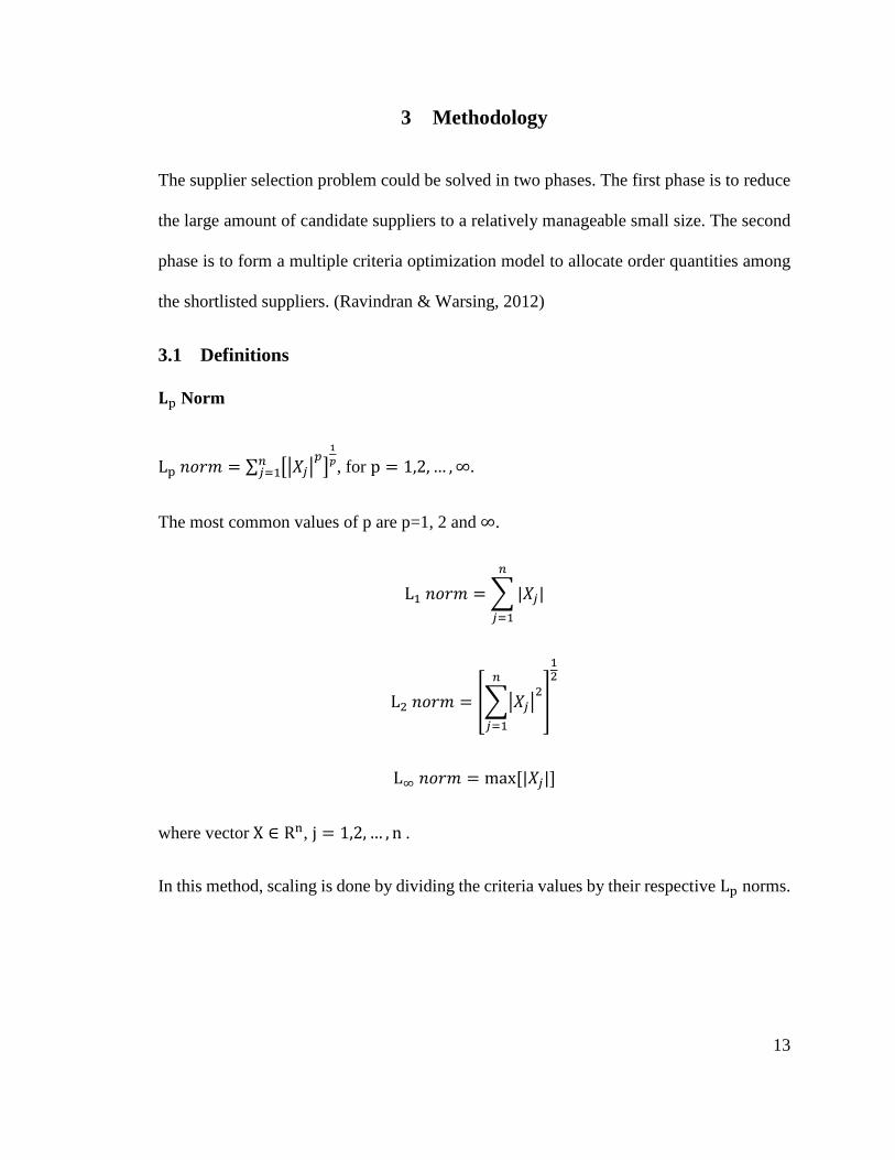
3 Methodology
The supplier selection problem could be solved in two phases. The first phase is to reduce
the large amount of candidate suppliers to a relatively manageable small size. The second
phase is to form a multiple criteria optimization model to allocate order quantities among
the shortlisted suppliers. (Ravindran & Warsing, 2012)
3.1 Definitions
𝐋𝐋p Norm
Lp 𝑛𝑛𝑛𝑛𝑛𝑛𝑛𝑛 = ∑ ��𝑋𝑋𝑗𝑗�𝑝𝑝�1𝑝𝑝𝑛𝑛
𝑗𝑗=1 , for p = 1,2, … ,∞.
The most common values of p are p=1, 2 and ∞.
L1 𝑛𝑛𝑛𝑛𝑛𝑛𝑛𝑛 = � |𝑋𝑋𝑗𝑗|𝑛𝑛
𝑗𝑗=1
L2 𝑛𝑛𝑛𝑛𝑛𝑛𝑛𝑛 = ���𝑋𝑋𝑗𝑗�2
𝑛𝑛
𝑗𝑗=1
�
12
L∞ 𝑛𝑛𝑛𝑛𝑛𝑛𝑛𝑛 = max [|𝑋𝑋𝑗𝑗|]
where vector X ∈ Rn, j = 1,2, … , n .
In this method, scaling is done by dividing the criteria values by their respective Lp norms.
13

Borda Count
This method is named after Jean Charles de Borda, an 18th century French physicist. The
method is defined as follows:
1. The n criteria are ranked 1 when most important, to n when least important. Criterion
ranked 1 gets n points, 2 gets n-1 points, and the last place gets 1 point.
2. Weights for the criteria are calculated as follows:
Criterion ranked 1 = ns
Criterion ranked 2 = n−1s
Criterion ranked n = 1s
where s is the sum of all the points s = n(n+1)2
.
AHP
The AHP was developed by (Saaty, 1980) and has been thoroughly discussed in (Ravindran
& Warsing, 2012). It is a multiple criteria decision making method for ranking alternatives.
In the supplier selection process, AHP includes not only quantitative but also qualitative
factors, such as financial stability, feeling of trust, etc. There are six steps to implement
AHP.
• Step 1: Carry out a pair-wise comparison between criteria using the 1-9 degree of
importance scale as shown Table 1.
14

Degree of Importance Definition
1 Equal importance
3 Weak importance of one over other
5 Essential or strong importance
7 Demonstrated importance 9 Absolute importance
2,4,6,8 Intermediate values between two adjacent judgments
Table 1 Degree of Importance Scale in AHP
The pair-wise comparison matrix for the criteria is given by A(n×n) = [𝑎𝑎𝑖𝑖𝑗𝑗], if there are n
criteria to evaluate. aij represents the relative importance of criterion i with respect to
criterion j. aii = 1 and aji = 1𝑎𝑎𝑖𝑖𝑖𝑖
.
Step 2: Compute the normalized weights for the main criteria. L1 norm is most commonly
used. The two step process for calculating the weights is presented as follows:
• Normalize each column of A matrix using L1 norm:
rij =𝑎𝑎𝑖𝑖𝑗𝑗
∑ 𝑎𝑎𝑖𝑖𝑗𝑗𝑛𝑛𝑖𝑖=1
• Average the normalized values across each row to get the criteria weights:
wi =∑ 𝑛𝑛𝑖𝑖𝑗𝑗𝑛𝑛𝑗𝑗=1
𝑛𝑛
15

Step 3: Check consistency of the pair-wise comparison matrix using Eigen value theory as
follows:
• Compute the vector AW, where A is the pair-wise comparison matrix and W is the
weight matrix. Let the vector X = (X1, X2, X3, … , Xn) denote the values of AW.
• Compute
𝜆𝜆𝑚𝑚𝑎𝑎𝑚𝑚 = 𝐴𝐴𝐴𝐴𝐴𝐴𝑛𝑛𝑎𝑎𝐴𝐴𝐴𝐴[𝑋𝑋1𝑊𝑊1
,𝑋𝑋2𝑊𝑊2
,𝑋𝑋3𝑊𝑊3
, … ,𝑋𝑋𝑛𝑛𝑊𝑊𝑛𝑛
]
• Consistency index (CI) is given by
CI =𝜆𝜆𝑚𝑚𝑎𝑎𝑚𝑚 − n
n − 1
The values of RI are listed in Table 2
Table 2 the Value of RI
Consistency ratio (CR) is defined as CR = CIRI
. If CR<0.15, the pair-wise
comparison matrix is consistent.
Step 4: Compute the relative importance of the sub-criteria in the same way as the process
done for the main criteria. Step 2 and Step 3 are performed for every pair of sub-criteria
with respect to their main criterion. The final weights of the sub-criteria are the product of
the weights calculated first in step 4 and its corresponding main criterion weight.
16

Step 5: Repeat Step 1, 2 and 3 to obtain:
• Pair-wise comparison of alternatives with respect to each criterion using the ratio
scale.
• Normalized scores of all alternatives with respect to each criterion. Note that a
S(m×m matrix is obtained, and Sij is noted as normalized score for alternative i with
respect to criterion j and m is the number of alternatives.
Step 6: Compute the total score (TS) for each alternative. TS(m×1) = 𝑆𝑆(𝑚𝑚×n)𝑊𝑊(𝑛𝑛×1), where
W is the weight vector obtained after step 4. Hence the alternatives will be ranked with the
TS.
Capacity Utilization
The percentage of the full capacity being utilized.
Fixed Cost
Fixed cost is a one-time cost that incurred if a supplier is used, irrespective of the number
of units bought from that supplier.
Less-Than-Truckload (LTL)
A quantity of freight which is less the required freight for a truckload. The historical
definition of LTL is the shipments of freight under 10,000 pounds.
Truckload (TL)
A quantity of freight which could fill a truck. The historical definition of TL is a shipment
of fright with 10,000 pounds or more.
17

Global and Local Optima
A global optimal solution for a specific model is a feasible solution which has an objective
value as good as or better than all other feasible solutions. The properties of constraints
and objective functions determine whether a globally optimal solution could be obtained.
Linear optimization models satisfy these properties.
A local optimal solution for a specific model is a feasible solution which has an objective
value as good as or better than all other feasible solutions in the immediate neighborhood.
Although no better solution could be found in the immediate neighborhood, a better
solution may exist at some distance away. Nonlinear optimization models may have several
local optima.
Convexity
A geometric definition of convexity is defined that when a function is convex, for any two
points on the function, a straight line connecting this two points lies entirely on or above
the function. For minimizing a convex function, a global optimal solution could be found.
Integer and Mixed Integer Linear Problems
Integer programming (IP) models are linear programming models with binary (0-1)
decision variables. Mixed integer programming (MIP) models refer to general IP models
which include regular integer variables (non 0-1) and continuous variables. An example of
MIP model is shown as follows:
18

Objective:
min�𝑎𝑎𝑗𝑗 𝑥𝑥𝑗𝑗𝑗𝑗∈𝐵𝐵
+ �𝑏𝑏𝑗𝑗𝑥𝑥𝑗𝑗𝑗𝑗∈𝐼𝐼
+ �𝑐𝑐𝑗𝑗𝑥𝑥𝑗𝑗𝑗𝑗∈𝐶𝐶
Constraints:
�𝑑𝑑𝑖𝑖𝑗𝑗𝑥𝑥𝑗𝑗𝑗𝑗∈𝐵𝐵
+ �𝐴𝐴𝑖𝑖𝑗𝑗𝑥𝑥𝑗𝑗𝑗𝑗∈𝐼𝐼
> 𝑓𝑓𝑖𝑖 (i = 1,2, … , m)
lj ≤ xj ≤ uj (𝑗𝑗 ∈ 𝐼𝐼)
xj ∈ {0,1} (𝑗𝑗 ∈ 𝐵𝐵)
xj ∈ 𝑖𝑖𝑛𝑛𝑖𝑖 (𝑗𝑗 ∈ 𝐼𝐼)
xj ∈ 𝑛𝑛𝐴𝐴𝑎𝑎𝑟𝑟 (𝑗𝑗 ∈ 𝐶𝐶)
where B is the set of 0-1 variables, I is the set of integer variables, and C is the set of
continuous variables. lj and uj are the lower and upper bound values for variable xj.
19

3.2 First Phase
In this thesis, considering the first phase, L∞ Norm is used to scale the criteria, Borda count
will be used to rank these criteria, the number of initial suppliers will be reduced, and AHP
will be conducted to rank the reduced suppliers.
3.3 Second Phase
In the second phase, an optimization model for final selection of suppliers and order
allocation including cross docking and cold chain constraints will be solved among the
shortlisted suppliers determined in the first phase.
3.3.1 Model
A supply chain may be made of several different companies. These companies could range
from suppliers to distribution centers to retailers. This thesis investigates a win-win
situation for both cross docking operators and the retailers.
The objective of the optimization model is to minimize the major costs in the cold supply
chain, namely the fixed and variable costs of the suppliers, the transportation costs, and the
value loss costs in cold chain subject to certain constraints. These constraints are based on
operating conditions of the cold chain cross docking and the terms of business between the
cross docking operator, the suppliers and the retailers.
The operations we aim to model include suppliers, a cross docking facility and retailers.
The cross docking facility receives products from suppliers, thereafter, products are
unloaded from inbound trucks, consolidated, and loaded onto the outbound trucks.
20

Figure 3 The Supply Chain for the Model
3.3.2 Assumptions
To mathematically formulate the operations of the supply chain shown in Figure 3, we
made some assumptions as follows:
1. The demand for product i is deterministic.
2. Lead time is not considered in this model. There is no lead time of delivery of products
to the next echelon.
3. Each supplier is responsible for getting items ready for pick up.
4. No shortage or delay occurs for picking up items.
5. The penalty costs of not being able to fulfill the demand are not included in the objective
function. All demands are met.
6. Charges of holding the inventory are ignored.
21

7. The optimal route for the movement of trucks from cross docking to retailers is pre-
determined.
8. Initial inventory is zero.
9. The outbound shipments are consolidated at the cross docking and hence consist of
various products received during the horizon.
10. All products shipped from the suppliers have the same initial quality.
3.3.3 Indices
Below are the indices used throughout the model.
I Index of product, i=1,2,…,n
T Index of time horizon, t=1,2,…,T
n Number of products managed by the cross docking facility in periods
t=1,2,…,T
J Index of potential suppliers for each product, j=1,2,…,J
3.3.4 Parameters
Below are some parameters used in the model.
𝑲𝑲𝒊𝒊,𝒋𝒋𝑰𝑰 Inbound cost per container of product i from supplier j
𝑲𝑲𝑶𝑶 Outbound cost per container
𝑪𝑪𝑶𝑶 Capacity of the outbound trucks
𝑪𝑪𝑰𝑰 Capacity of the inbound trucks
𝑪𝑪𝒊𝒊,𝒋𝒋 Capacity of supplier j for product i in the time horizon T
𝒗𝒗𝒊𝒊 Volume occupied by product i
22

𝝀𝝀𝒊𝒊 Per period demand of product i at the retailer
𝑼𝑼𝒊𝒊,𝒋𝒋 Unit price of product i shipped from supplier j
𝑭𝑭𝒊𝒊,𝒋𝒋 Fixed costs of using supplier j for product i. It will occur no matter
supplier j has been used in which period
𝒉𝒉𝒊𝒊,𝒋𝒋𝑰𝑰 Value lost per unit of product i in inbound transportation from supplier
j
𝒉𝒉𝒊𝒊𝑪𝑪𝑪𝑪 Value lost per unit of product i in cross docking
𝒉𝒉𝒊𝒊𝑶𝑶 Value lost per unit of product i in the outbound transportation
𝑪𝑪𝒊𝒊,𝒋𝒋 Defect percentage of product i from supplier j
3.3.5 Decision Variables
We introduce the decision variables and give their definitions below.
𝜶𝜶𝒊𝒊,𝒋𝒋,𝒕𝒕 Fraction of the total horizon demand of product i shipped from supplier
j to the cross docking in period t
Note: The total horizon demand of product 𝑖𝑖 = 𝜆𝜆𝑖𝑖𝑇𝑇
𝝎𝝎𝒊𝒊,𝒕𝒕 Fraction of the total horizon demand of product i shipped from the
cross docking to the retailer in period t
𝒏𝒏𝒊𝒊,𝒋𝒋,𝒕𝒕𝑰𝑰 Number of inbound shipments of product i from supplier j in period t
𝒏𝒏𝒕𝒕𝑶𝑶 Number of outbound shipments in period t
𝜹𝜹𝒊𝒊,𝒋𝒋 1, if supplier j is used
0, otherwise
23

3.3.6 Problem Formulation
We present the methodology for formulating the math program in this section.
Objective Function
Minimizing the sum of fixed costs of the suppliers, variable costs of the suppliers, inbound
transportation costs, outbound transportation costs, values loss costs in cold chain.
Minimize Total Cost =
��𝐹𝐹𝑖𝑖,𝑗𝑗𝛿𝛿𝑖𝑖,𝑗𝑗
𝐽𝐽
𝑗𝑗=1
𝑛𝑛
𝑖𝑖=1
+ ���𝛼𝛼𝑖𝑖,𝑗𝑗,𝑡𝑡𝑈𝑈𝑖𝑖,𝑗𝑗(𝜆𝜆𝑖𝑖𝑇𝑇)𝑇𝑇
𝑡𝑡=1
𝐽𝐽
𝑗𝑗=1
𝑛𝑛
𝑖𝑖=1
+ ���𝑛𝑛𝑖𝑖,𝑗𝑗,𝑡𝑡𝐼𝐼 𝐾𝐾𝑖𝑖,𝑗𝑗𝐼𝐼
𝑇𝑇
𝑡𝑡=1
𝐽𝐽
𝑗𝑗=1
𝑛𝑛
𝑖𝑖=1
+ �𝑛𝑛𝑡𝑡𝑂𝑂𝑘𝑘𝑂𝑂𝑇𝑇
𝑡𝑡=1
+ ���𝛼𝛼𝑖𝑖,𝑗𝑗,𝑡𝑡𝐷𝐷𝑖𝑖,𝑗𝑗(𝜆𝜆𝑖𝑖𝑇𝑇)(ℎ𝑖𝑖,𝑗𝑗𝐼𝐼 + ℎ𝑖𝑖𝐶𝐶𝐶𝐶 + ℎ𝑖𝑖𝑂𝑂)𝑇𝑇
𝑡𝑡=1
𝐽𝐽
𝑗𝑗=1
𝑛𝑛
𝑖𝑖=1
Constraints
1. Receive and Ship all Products in Cross Docking:
��𝛼𝛼𝑖𝑖,𝑗𝑗,𝑡𝑡
𝑇𝑇
𝑡𝑡=1
𝐽𝐽
𝑗𝑗=1
= 1,∀𝑖𝑖
�𝜔𝜔𝑖𝑖,𝑡𝑡
𝑇𝑇
𝑡𝑡=1
= 1,∀𝑖𝑖
2. Capacity Constraints of the suppliers:
�𝛼𝛼𝑖𝑖,𝑗𝑗,𝑡𝑡(𝜆𝜆𝑖𝑖𝑇𝑇) ≤𝑇𝑇
𝑡𝑡=1
𝐶𝐶𝑖𝑖,𝑗𝑗𝛿𝛿𝑖𝑖,𝑗𝑗,∀i, j
24

3. Inbound Transportation:
vi × 𝛼𝛼𝑖𝑖,𝑗𝑗,𝑡𝑡 × (𝜆𝜆𝑖𝑖𝑇𝑇) ≤ 𝑛𝑛𝑖𝑖,𝑗𝑗,𝑡𝑡𝐼𝐼 × 𝐶𝐶𝐼𝐼 ,∀𝑖𝑖, 𝑗𝑗, 𝑖𝑖
The inbound transportation constraint restrict the shipping capacity not being violated on
the inbound side.
ni,j,t𝐼𝐼 ≤ 𝑀𝑀𝛿𝛿𝑖𝑖,𝑗𝑗,∀𝑖𝑖, 𝑗𝑗
where M is a very large real number. This constraint ensures that, when a supplier j not be
chosen, the inbound shipment number for that supplier would be zero.
4. Outbound Transportation
�𝐴𝐴𝑖𝑖 × 𝜔𝜔𝑖𝑖,𝑡𝑡 × (𝜆𝜆𝑖𝑖𝑇𝑇) ≤ 𝑛𝑛𝑡𝑡𝑂𝑂 × 𝐶𝐶𝑂𝑂𝑛𝑛
𝑖𝑖=1
,∀𝑖𝑖
The outbound transportation constraint restricts the shipping capacity not being violated
on the outbound side.
5. Binary, Integer and Non-negativity Constraints
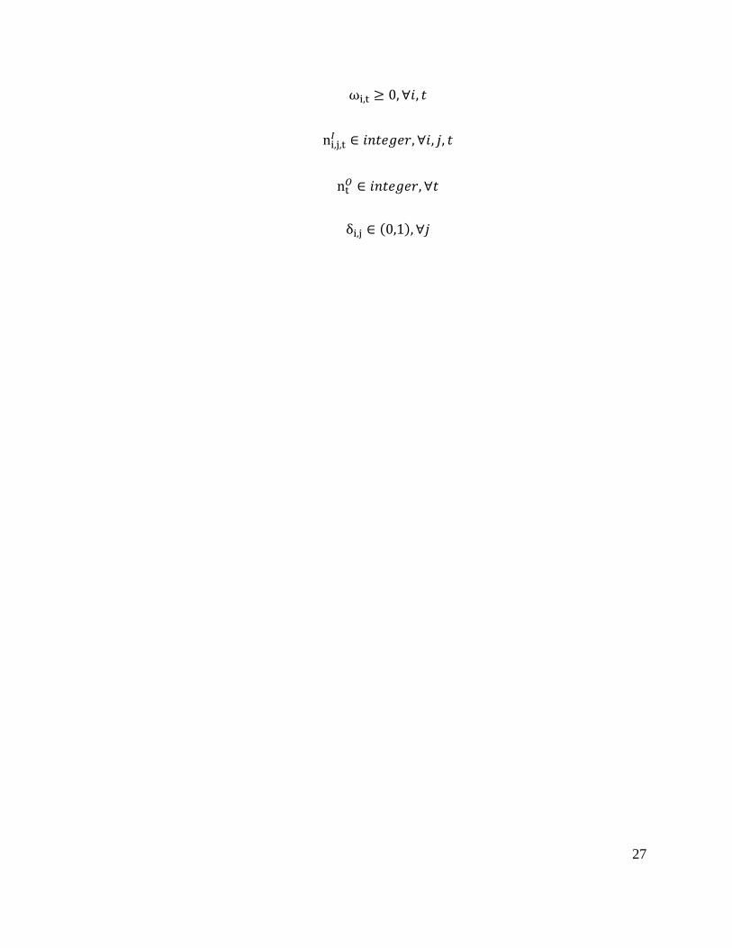
αi,j,t ≥ 0,∀𝑖𝑖, 𝑗𝑗, 𝑖𝑖
ωi,t ≥ 0,∀𝑖𝑖, 𝑖𝑖
ni,j,t𝐼𝐼 ∈ 𝑖𝑖𝑛𝑛𝑖𝑖𝐴𝐴𝐴𝐴𝐴𝐴𝑛𝑛,∀𝑖𝑖, 𝑗𝑗, 𝑖𝑖
nt𝑂𝑂 ∈ 𝑖𝑖𝑛𝑛𝑖𝑖𝐴𝐴𝐴𝐴𝐴𝐴𝑛𝑛,∀𝑖𝑖
δi,j ∈ (0,1),∀𝑖𝑖, 𝑗𝑗
25

Final Mixed Integer Linear Optimization Model:
Minimize Total Cost =
�𝐹𝐹𝑖𝑖,𝑗𝑗𝛿𝛿𝑖𝑖,𝑗𝑗
𝐽𝐽
𝑗𝑗=1
+ ���𝛼𝛼𝑖𝑖,𝑗𝑗,𝑡𝑡𝑈𝑈𝑖𝑖,𝑗𝑗(𝜆𝜆𝑖𝑖𝑇𝑇)𝑇𝑇
𝑡𝑡=1
𝐽𝐽
𝑗𝑗=1
𝑛𝑛
𝑖𝑖=1
+ ���𝑛𝑛𝑖𝑖,𝑗𝑗,𝑡𝑡𝐼𝐼 𝐾𝐾𝑖𝑖,𝑗𝑗𝐼𝐼
𝑇𝑇
𝑡𝑡=1
𝐽𝐽
𝑗𝑗=1
𝑛𝑛
𝑖𝑖=1
+ �𝑛𝑛𝑡𝑡𝑂𝑂𝑘𝑘𝑂𝑂𝑇𝑇
𝑡𝑡=1
+ ���𝛼𝛼𝑖𝑖,𝑗𝑗,𝑡𝑡𝐷𝐷𝑖𝑖,𝑗𝑗(𝜆𝜆𝑖𝑖𝑇𝑇)(ℎ𝑖𝑖,𝑗𝑗𝐼𝐼 + ℎ𝑖𝑖𝐶𝐶𝐶𝐶 + ℎ𝑖𝑖𝑂𝑂)𝑇𝑇
𝑡𝑡=1
𝐽𝐽
𝑗𝑗=1
𝑛𝑛
𝑖𝑖=1
Subject to
��𝛼𝛼𝑖𝑖,𝑗𝑗,𝑡𝑡
𝑇𝑇
𝑡𝑡=1
𝐽𝐽
𝑗𝑗=1
= 1,∀𝑖𝑖
�𝜔𝜔𝑖𝑖,𝑡𝑡
𝑇𝑇
𝑡𝑡=1
= 1,∀𝑖𝑖
�𝛼𝛼𝑖𝑖,𝑗𝑗,𝑡𝑡(𝜆𝜆𝑖𝑖𝑇𝑇) ≤𝑇𝑇
𝑡𝑡=1
𝐶𝐶𝑖𝑖,𝑗𝑗𝛿𝛿𝑖𝑖,𝑗𝑗,∀i, j
vi × 𝛼𝛼𝑖𝑖,𝑗𝑗,𝑡𝑡 × (𝜆𝜆𝑖𝑖𝑇𝑇) ≤ 𝑛𝑛𝑖𝑖,𝑗𝑗,𝑡𝑡𝐼𝐼 × 𝐶𝐶𝐼𝐼 ,∀𝑖𝑖, 𝑗𝑗, 𝑖𝑖
ni,j,t𝐼𝐼 ≤ 𝑀𝑀𝛿𝛿𝑖𝑖,𝑗𝑗,∀𝑖𝑖, 𝑗𝑗
where M is a very large real number.
�𝐴𝐴𝑖𝑖 × 𝜔𝜔𝑖𝑖,𝑡𝑡 × (𝜆𝜆𝑖𝑖𝑇𝑇) ≤ 𝑛𝑛𝑡𝑡𝑂𝑂 × 𝐶𝐶𝑂𝑂𝑛𝑛
𝑖𝑖=1
,∀𝑖𝑖
αi,j,t ≥ 0,∀𝑖𝑖, 𝑗𝑗, 𝑖𝑖 26
ωi,t ≥ 0,∀𝑖𝑖, 𝑖𝑖
ni,j,t𝐼𝐼 ∈ 𝑖𝑖𝑛𝑛𝑖𝑖𝐴𝐴𝐴𝐴𝐴𝐴𝑛𝑛,∀𝑖𝑖, 𝑗𝑗, 𝑖𝑖
nt𝑂𝑂 ∈ 𝑖𝑖𝑛𝑛𝑖𝑖𝐴𝐴𝐴𝐴𝐴𝐴𝑛𝑛,∀𝑖𝑖
δi,j ∈ (0,1),∀𝑗𝑗
27

4 Example and Discussions
In this section, a pilot problem with 2 products, 2 suppliers for each product in a time
horizon spanning 3 days is presented to illustrate how the supplier selection is carried out
using the two-phase methodology proposed in Chapter 3.
4.1 First Phase
There are 15 potential suppliers for product 1 which are randomly chosen from top 200
suppliers for Product 1. And there are also 15 potential suppliers for Product 2 which are
randomly chosen from top 200 suppliers for Product 2. We firstly reduce the suppliers to
10, 5 for Product 1 and 5 for Product 2 by using L∞ Norm and Borda Count. Secondly,
ranking these reduced suppliers for each product by AHP, and obtaining top 2 suppliers for
each product. Table 3 and Table 4 show the suppliers chosen in the first place for Product
1 and Product 2 respectively. Data used in the First Phase is partially from one of my course
project, Goal Programming Approaches of Franchise Selection, other team members in this
project are Xuan Li, Maiteng Pornthip, and Vara-Urairat Putthipan.
28

Supplier No. Rank in Top 200 1 1 2 3 3 4 4 5 5 12 6 15 7 38 8 39 9 43 10 46 11 48 12 53 13 54 14 67 15 80
Table 3 Potential Suppliers for Product 1
Supplier No. Rank in Top 200 1 17 2 18 3 34 4 47 5 84 6 125 7 136 8 137 9 142 10 145 11 150 12 180 13 186 14 188 15 195
Table 4 Potential Suppliers for Product 2
29

Screening Process with 𝐋𝐋∞ Norm and Borda Count
Fourteen criteria are considered in this stage and are denoted as criterion 1, criterion 2,
criterion 3 and etc. Criterion 1 to 8 and criterion 14 need to be minimized, while criterion
9 to criterion 13 need to be maximized.
Using L∞ Norm and Borda Count here is trying to reduce the initial suppliers. This makes
it much easier for us to do AHP since we will reduce the suppliers to ten, five for product
1 and five for product 2. We use L∞ Norm to scale and use Borda Count to rank the
suppliers.
• Define the L∞ Norm of each criterion and sub-criterion. L∞ Norm is calculated as:
L∞ 𝑁𝑁𝑛𝑛𝑛𝑛𝑛𝑛 = max [|𝑋𝑋𝑗𝑗|]
To do the scaling, the criterion values is divided by their respective L∞ Norm. Table
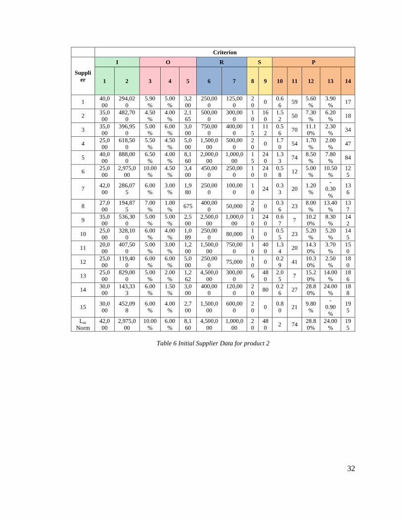
5 and Table 6 show the potential supplier criteria data for product 1 and product 2
respectively. Table 7 and Table 8 list the normalized criterion data for each product.
30

Criterion
Supplier
I O R S P
1 2 3 4 5 6 7 8 9 10 11 12 13 14
1 45,000
986,350
4.00%
4.00%
57,600 0 750,00
0 20 2160
2.73 59 12.2
0% 4.30% 1
2 45,000
1,264,900
5.00%
5.00%
2,160
1,500,000
750,000 20 44
8 1.25 62 7.00
% 4.60% 3
3 15,000
157,775
8.00%
4.50%
13,286 30,000 195,00
0 20 112
0.47 40 9.00
% 6.70% 4
4 50,000
1,360,600
4.50%
4.00%
7,500
1,500,000
500,000 20 44
0 1.22 55 3.60
% 3.90% 5
5 45,000
1,148,300
5.50%
4.50%
10,000
1,500,000
750,000 25 39
2 1.30 50 6.80
% 0.60% 12
6 25,000
265,825
5.50%
4.00%
15,435
250,000 75,000 10 0 0.7
2 47 6.40%
5.30% 15
7 50,000
1,208,900
5.00%
5.00%
10,000
1,500,000
750,000 0 24
0 1.37 32 4.70
% 1.30% 38
8 15,000
733,000
4.00%
4.20%
12,500
1,000,000
180,700 20 28
0 0.88 49
-1.10%
-2.30%
39
9 0 124,823
5.00%
9.00%
1,432 50,000 150,00
0 10 120
0.68 29 10.6
0% 7.20% 43
10 50,000
2,021,500
5.00%
4.00%
20,085
6,000,000
2,500,000 10 44
0 2.96 45 3.80
% 1.00% 46
11 0 1,178,556
4.00%
4.00%
20,000
1,000,000
350,000 20 15
2 1.48 51 3.20
% 0.20% 48
12 35,000
1,034,600
5.00%
4.00%
36,000
1,000,000
500,000 20 44
0 1.06 22 13.3
0% 1.20% 53
13 10,000
1,437,900
4.00%
5.00%
20,150
1,000,000
300,000 20 56
0 1.12 53 5.50
% 1.20% 54
14 35,000
1,196,500
4.00%
5.50% 0 1,000,0
00 300,00
0 20 0 1.21 30 7.50
% 4.30% 67
15 25,000
281,200
6.00%
1.50%
10,500
1,500,000
500,000 10 11
2 0.98 12 19.6
0% 21.60% 80
L∞ Norm
50,000
2,021,500
8.00%
9.00%
57,600
6,000,000
2,500,000 25
2,160
3 62 19.60%
21.60% 80
Table 5 Potential Suppliers for Product 2
31
Criterion
Supplier
I O R S P
1 2 3 4 5 6 7 8 9 10 11 12 13 14
1 40,000
294,020
5.90%
5.00%
3,200
250,000
125,000
20 0 0.6
6 59 5.60%
3.90% 17
2 35,000
482,700
4.50%
4.00%
2,165
500,000
300,000
10
160
1.52 50 7.30
% 6.20% 18
3 35,000
396,950
5.00%
6.00%
3,000
750,000
400,000
15
112
0.56 70 11.1
0% 2.30% 34
4 25,000
618,500
5.50%
4.50%
5,000
1,500,000
500,000
20 0 1.7
0 54 1.70%
2.00% 47
5 40,000
888,000
6.50%
4.00%
8,160
2,000,000
1,000,000
15
240
1.33 74 8.50
% 7.80% 84
6 25,000
2,975,000
10.00%
4.50%
3,400
450,000
250,000
10
240
0.58 12 5.00
% 10.50
% 125
7 42,000
286,075
6.00%
3.00%
1,980
250,000
100,000
10 24 0.3
3 20 1.20%
-0.30%
136
8 27,000
194,875
7.00%
1.00% 675 400,00
0 50,000 20 0 0.3
6 23 8.00%
13.40%
137
9 35,000
536,300
5.00%
5.00%
2,500
2,500,000
1,000,000
10
240
0.67 7 10.2
0% 8.30%
142
10 25,000
328,100
6.00%
4.00%
1,089
250,000 80,000 1
0 0 0.55 23 5.20
% 5.20%
145
11 20,000
407,500
5.00%
3.00%
1,200
1,500,000
750,000
10
400
1.34 20 14.3
0% 3.70%
150
12 25,000
119,400
6.00%
6.00%
5,000
250,000 75,000 1
0 0 0.29 41 10.3
0% 2.50%
180
13 25,000
829,000
5.00%
2.00%
1,262
4,500,000
300,000 6 48
0 2.05 7 15.2
0% 14.00
% 186
14 30,000
143,333
6.00%
1.50%
3,000
400,000
120,000
20 80 0.2
6 27 28.80%
24.00%
188
15 30,000
452,098
6.00%
4.00%
2,700
1,500,000
600,000
20 0 0.8
0 21 9.80%
-0.90%
195
L∞ Norm
42,000
2,975,000
10.00%
6.00%
8,160
4,500,000
1,000,000
20
480 2 74 28.8
0% 24.00
% 195
Table 6 Initial Supplier Data for product 2
32

Criterion
Supplier I O R S P
1 2 3 4 5 6 7 8 9 10 11 12 13 14 1 0.90 0.49 0.50 0.44 1.00 0.00 0.30 0.80 1.00 0.92 0.95 0.62 0.20 0.01
2 0.90 0.63 0.63 0.56 0.04 0.25 0.30 0.80 0.21 0.42 1.00 0.36 0.21 0.04
3 0.30 0.08 1.00 0.50 0.23 0.01 0.08 0.80 0.05 0.16 0.65 0.46 0.31 0.05
4 1.00 0.67 0.56 0.44 0.13 0.25 0.20 0.80 0.20 0.41 0.89 0.18 0.18 0.06
5 0.90 0.57 0.69 0.50 0.17 0.25 0.30 1.00 0.18 0.44 0.81 0.35 0.03 0.15
6 0.50 0.13 0.69 0.44 0.27 0.04 0.03 0.40 0.00 0.24 0.76 0.33 0.25 0.19
7 1.00 0.60 0.63 0.56 0.17 0.25 0.30 0.00 0.11 0.46 0.52 0.24 0.06 0.48
8 0.30 0.36 0.50 0.47 0.22 0.17 0.07 0.80 0.13 0.30 0.79 -0.06
-0.11 0.49
9 0.00 0.06 0.63 1.00 0.02 0.01 0.06 0.40 0.06 0.23 0.47 0.54 0.33 0.54
10 1.00 1.00 0.63 0.44 0.35 1.00 1.00 0.40 0.20 1.00 0.73 0.19 0.05 0.58
11 0.00 0.58 0.50 0.44 0.35 0.17 0.14 0.80 0.07 0.50 0.82 0.16 0.01 0.60
12 0.70 0.51 0.63 0.44 0.63 0.17 0.20 0.80 0.20 0.36 0.35 0.68 0.06 0.66
13 0.20 0.71 0.50 0.56 0.35 0.17 0.12 0.80 0.26 0.38 0.85 0.28 0.06 0.68
14 0.70 0.59 0.50 0.61 0.00 0.17 0.12 0.80 0.00 0.41 0.48 0.38 0.20 0.84
15 0.50 0.14 0.75 0.17 0.18 0.25 0.20 0.40 0.05 0.33 0.19 1.00 1.00 1.00
Table 7 Normalized Supplier Data for Product 1
Criterion
Supplier I O R S P
1 2 3 4 5 6 7 8 9 10 11 12 13 14 1 0.95 0.10 0.59 0.83 0.39 0.06 0.13 1.00 0.00 0.32 0.80 0.19 0.16 0.09
2 0.83 0.16 0.45 0.67 0.27 0.11 0.30 0.50 0.33 0.74 0.68 0.25 0.26 0.09
3 0.83 0.13 0.50 1.00 0.37 0.17 0.40 0.75 0.23 0.28 0.95 0.39 0.10 0.17
4 0.60 0.21 0.55 0.75 0.61 0.33 0.50 1.00 0.00 0.83 0.73 0.06 0.08 0.24
5 0.95 0.30 0.65 0.67 1.00 0.44 1.00 0.75 0.50 0.65 1.00 0.30 0.33 0.43
6 0.60 1.00 1.00 0.75 0.42 0.10 0.25 0.50 0.50 0.28 0.16 0.17 0.44 0.64
7 1.00 0.10 0.60 0.50 0.24 0.06 0.10 0.50 0.05 0.16 0.27 0.04 -0.01 0.70
8 0.64 0.07 0.70 0.17 0.08 0.09 0.05 1.00 0.00 0.17 0.31 0.28 0.56 0.70
9 0.83 0.18 0.50 0.83 0.31 0.56 1.00 0.50 0.50 0.33 0.09 0.35 0.35 0.73
10 0.60 0.11 0.60 0.67 0.13 0.06 0.08 0.50 0.00 0.27 0.31 0.18 0.22 0.74
11 0.48 0.14 0.50 0.50 0.15 0.33 0.75 0.50 0.83 0.66 0.27 0.50 0.15 0.77
12 0.60 0.04 0.60 1.00 0.61 0.06 0.08 0.50 0.00 0.14 0.55 0.36 0.10 0.92
13 0.60 0.28 0.50 0.33 0.15 1.00 0.30 0.30 1.00 1.00 0.09 0.53 0.58 0.95
14 0.71 0.05 0.60 0.25 0.37 0.09 0.12 1.00 0.17 0.12 0.36 1.00 1.00 0.96
15 0.71 0.15 0.60 0.67 0.33 0.33 0.60 1.00 0.00 0.39 0.28 0.34 -0.04 1.00
Table 8 Normalized Supplier Data for Product 2
33

• Ask decision maker (DM) for preference information between pairs of criteria. In
the pairwise comparison matrix, pij = 1 when i is preferred to j, meanwhile, pji =
0, and vise versa. pij = pji = 1 when i and j are equally preferred. pii = 1 all the
time. The preference matrix is shown in Table 9.
Criterion 1 2 3 4 5 6 7 8 9 10 11 12 13 14 1 1 0 0 0 0 0 0 0 0 0 0 0 0 0 2 1 1 1 1 1 1 1 1 1 1 1 1 1 1 3 1 0 1 1 1 1 1 1 1 1 1 1 1 1 4 1 0 0 1 1 1 1 1 1 1 1 1 1 1 5 1 0 0 0 1 0 0 0 0 0 1 0 0 0 6 1 0 0 0 1 1 1 0 1 0 1 0 1 1 7 1 0 0 0 1 0 1 0 1 0 1 0 1 1 8 1 0 0 0 1 1 1 1 1 0 1 0 0 1 9 1 0 0 0 1 0 0 0 1 0 0 0 0 0
10 1 0 0 0 1 1 1 1 1 1 1 1 1 1 11 1 0 0 0 0 0 0 0 1 0 1 0 0 0 12 1 0 0 0 1 1 1 1 1 0 1 1 1 0 13 1 0 0 0 1 0 0 1 1 0 1 0 1 0 14 1 0 0 0 1 0 0 0 1 0 1 1 1 1
Table 9 Preference Matrix of each Criterion
• Rank criteria and get weights using Borda Count, as listed in Table 10.
Criterion 1 2 3 4 5 6 7 8 9 10 11 12 13 14 Borda Count Rank
1 14 13 12 3 8 7 8 3 11 3 9 6 7
Weight
0.010
0.133
0.124
0.114
0.029
0.076
0.067
0.076
0.029
0.105
0.029
0.086
0.057
0.067
Table 10 Borda Count Rank and Weight of each Criterion
34

• Get the score of each supplier. For a supplier, the score is getting from the sum of
the product of each normalized criterion and its respective weight. If the criterion
needs to be minimized, multiply it by -1 first. Table 11 and Table 12 show the score
of suppliers for each product.
Supplier Score Rank 1 -0.080 1 15 -0.085 2 6 -0.125 3 9 -0.167 4 3 -0.177 5 2 -0.215 6 7 -0.215 7 4 -0.221 8 11 -0.231 9 12 -0.237 10 8 -0.237 11 5 -0.251 12 14 -0.254 13 13 -0.260 14 10 -0.342 15
Table 11 Score and Rank of Suppliers for Product 1
35

Supplier Score Rank
2 -0.099 1 14 -0.111 2 13 -0.115 3 11 -0.159 4 8 -0.173 5 10 -0.207 6 1 -0.214 7 3 -0.219 8 7 -0.227 9 4 -0.238 10 12 -0.259 11 5 -0.266 12 9 -0.292 13 15 -0.319 14 6 -0.377 15
Table 12 Score and Rank of Suppliers for Product 2
• Thus we choose Supplier 1, 15, 6, 9, and 3 for Product 1, while Supplier 2, 14, 13,
11, and 8 for Product 2 at this stage.
Criterion Weights and Ranking with AHP
Here we will reduce the 5 suppliers to 2 for each product. The motivation to use AHP to
rank suppliers is that this technique allows the selection to involve the assessment not only
numerical but also intangible factors. Figure 4 shows the supplier selection criteria in AHP
used for this example.
36
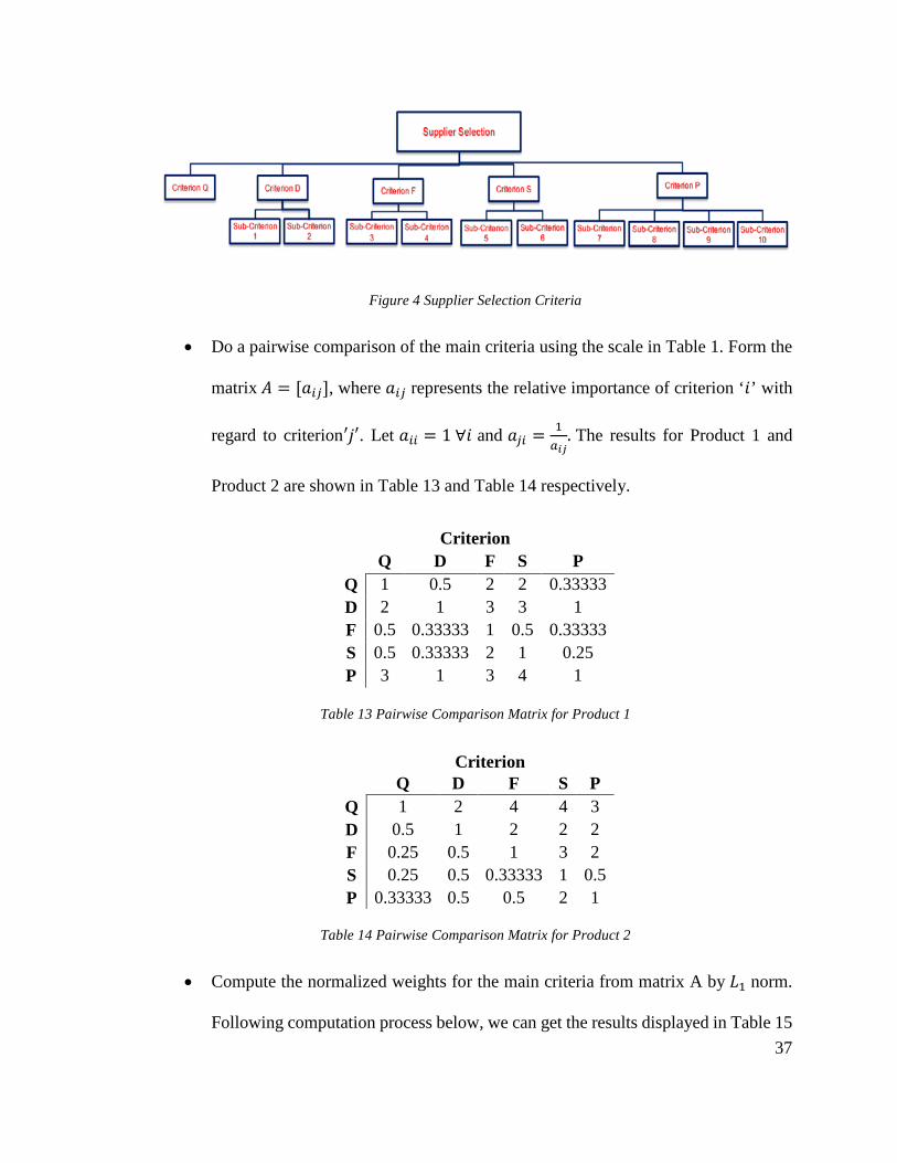
Figure 4 Supplier Selection Criteria
• Do a pairwise comparison of the main criteria using the scale in Table 1. Form the
matrix 𝐴𝐴 = [𝑎𝑎𝑖𝑖𝑗𝑗], where 𝑎𝑎𝑖𝑖𝑗𝑗 represents the relative importance of criterion ‘𝑖𝑖’ with
regard to criterion′𝑗𝑗′. Let 𝑎𝑎𝑖𝑖𝑖𝑖 = 1 ∀𝑖𝑖 and 𝑎𝑎𝑗𝑗𝑖𝑖 = 1𝑎𝑎𝑖𝑖𝑖𝑖
. The results for Product 1 and
Product 2 are shown in Table 13 and Table 14 respectively.
Criterion Q D F S P
Q 1 0.5 2 2 0.33333 D 2 1 3 3 1 F 0.5 0.33333 1 0.5 0.33333 S 0.5 0.33333 2 1 0.25 P 3 1 3 4 1
Table 13 Pairwise Comparison Matrix for Product 1
Criterion Q D F S P
Q 1 2 4 4 3 D 0.5 1 2 2 2 F 0.25 0.5 1 3 2 S 0.25 0.5 0.33333 1 0.5 P 0.33333 0.5 0.5 2 1
Table 14 Pairwise Comparison Matrix for Product 2
• Compute the normalized weights for the main criteria from matrix A by 𝐿𝐿1 norm.
Following computation process below, we can get the results displayed in Table 15 37

and Table 16: Compute 𝑛𝑛𝑖𝑖𝑗𝑗 = 𝑎𝑎𝑖𝑖𝑖𝑖∑ 𝑎𝑎𝑖𝑖𝑖𝑖𝑛𝑛𝑖𝑖=1
, then average the 𝑛𝑛𝑖𝑖𝑗𝑗 values to get the weights,
𝑤𝑤𝑖𝑖 =∑ 𝑟𝑟𝑖𝑖𝑖𝑖𝑖𝑖
𝑛𝑛.
Normalization
Weights
Q D F S P
Q 0.143 0.158 0.182 0.190 0.114 0.157 D 0.286 0.316 0.273 0.286 0.343 0.301 F 0.071 0.105 0.091 0.048 0.114 0.086 S 0.071 0.105 0.182 0.095 0.086 0.108 P 0.429 0.316 0.273 0.381 0.343 0.348
Table 15 Normalized Matrix for Product 1
Normalization
Weights
Q D F S P
Q 0.429 0.444 0.511 0.333 0.353 0.414 D 0.214 0.222 0.255 0.167 0.235 0.219 F 0.107 0.111 0.128 0.250 0.235 0.166 S 0.107 0.111 0.043 0.083 0.059 0.081 P 0.143 0.111 0.064 0.167 0.118 0.120
Table 16 Normalized Matrix for Product 2
Pairwise comparison and normalized weights are continuously performed
throughout every criteria and sub-criteria. Table 17 shows the weights of each
criterion for 2 products. The final weight of a sub-criterion is the product of the
weights with the corresponding branch.
38

Criterion/Sub-criterion Weight Product 1 Product 2 Q 0.157 0.414 D 0.156 0.153
- Sub-Criterion 1 0.145 0.066 - Sub-Criterion 2 0.029 0.055
F 0.057 0.111 - Sub-Criterion 3 0.027 0.054 - Sub-Criterion 4 0.081 0.027
S 0.158 0.019 - Sub-Criterion 5 0.090 0.054 - Sub-Criterion 6 0.051 0.035
P 0.048 0.013 - Sub-Criterion 7 0.157 0.414 - Sub-Criterion 8 0.156 0.153 - Sub-Criterion 9 0.145 0.066 - Sub-Criterion 10 0.029 0.055
Table 17 Criterion Weights
• Check consistency of the pairwise comparison matrix, using the Consistency Index
(CI) and the Consistency Ratio (CR). AHP has a procedure to check the consistency
of the DM's response. If the DM is perfectly consistent, then, A (before
normalization) has the following property:
If A is perfectly consistent then 𝜆𝜆𝑚𝑚𝑎𝑎𝑚𝑚 = 𝑛𝑛; where 𝜆𝜆𝑚𝑚𝑎𝑎𝑚𝑚 = 𝐴𝐴𝐴𝐴𝐴𝐴𝑛𝑛𝑎𝑎𝐴𝐴𝐴𝐴[𝐴𝐴1 • ∙ 𝑤𝑤/𝑤𝑤1,
𝐴𝐴2 • ∙ 𝑤𝑤/𝑤𝑤2, … ,𝐴𝐴𝑛𝑛 • ∙ 𝑤𝑤/𝑤𝑤𝑛𝑛, ]. To measure the degree of inconsistency, we use the
following indicators:
𝐶𝐶𝐼𝐼 =𝜆𝜆𝑚𝑚𝑎𝑎𝑚𝑚 − 𝑛𝑛𝑛𝑛 − 1
;𝐶𝐶𝐶𝐶 =𝐶𝐶𝐼𝐼𝐶𝐶𝐼𝐼
39

where RI is a random index, obtained from Table 2. If CR<0.1, the pairwise
comparison matrix would be accepted.
Finally, we check the consistency of pairwise comparison matrix for Product 1 and
Product 2, and they are all acceptable. Table 18 and Table 19 show the results:
Consistency Check AW 𝛌𝛌 0.811 5.153 𝛌𝛌𝐦𝐦𝐦𝐦𝐦𝐦 5.122 1.545 5.141 CI 0.031 0.435 5.062 RI 1.110 0.546 5.057 CR 0.028 1.810 5.200 Acceptance Y
Table 18 Consistency Check for Product 1
Consistency Check AW 𝛌𝛌 2.200 5.314 𝛌𝛌𝐦𝐦𝐦𝐦𝐦𝐦 5.192 1.160 5.304 CI 0.048 0.862 5.184 RI 1.110 0.409 5.076 CR 0.043 0.612 5.083 Acceptance Y
Table 19 Consistency Check for Product 2
At this point, we should proceed to rank all the suppliers by comparing the suppliers
with regard to each criterion using AHP. The column of Score Matrix (S) is formed
by the weights computed for each criterion. The Total Score (TS) of the suppliers
is determined by Equation shown below, where w corresponds to the criteria
weights, and S represents the Score Matrix. The suppliers are ranked by their TS
values, the higher the better.
40

𝑇𝑇𝑆𝑆 = �[𝑆𝑆 × 𝑤𝑤]11
𝑖𝑖=1
The results are shown in Table 20 and Table 21:
Supplier Total Score Rank
1 0.297 1 15 0.225 2 9 0.189 3 6 0.149 4 3 0.141 5
Table 20 AHP Rank for Product 1
Supplier Total Score Rank
14 0.299 1 8 0.257 2 2 0.164 3 11 0.142 4 13 0.139 5
Table 21 AHP Rank for Product 2
• Therefore, we choose Supplier 1 and Supplier 15 for Product 1, while choosing
Supplier 14 and Supplier 8 for Product 2 up to this stage.
41

4.2 Second Phase
For a better illustration, we match the reduced suppliers for Product 1 and Product 2 with
Supplier 1 and Supplier 2 for Product 1, and Supplier 1 and Supplier 2 for Product 2
correspondingly, as presented in Table 22.
Product 1 Noted as Product 2 Noted as
Supplier 1 Supplier 1 Supplier 14 Supplier 1
Supplier 15 Supplier 2 Supplier 8 Supplier 2
Table 22 Notation of Reduced Suppliers
The parameter values are chosen as:
n (Number of Products) = 2;
T (Time horizon) = 3 days;
J (Number of suppliers for each product) = 2;
𝐾𝐾1,1𝐼𝐼 ,𝐾𝐾1,2
𝐼𝐼 ,𝐾𝐾2,1𝐼𝐼 ,𝐾𝐾2,2
𝐼𝐼 (Cost of an inbound shipment for Product i from Supplier j) = $150,
$100, $100, $200 per shipment for Product 1, 2;
𝐾𝐾𝑂𝑂 (Cost of an outbound shipment) = $2000 per outbound shipment;
𝐶𝐶𝑂𝑂 (Outbound capacity) = 500 units;
𝐶𝐶𝐼𝐼 (Inbound capacity) = 500 units;
𝐶𝐶1,1,𝐶𝐶1,2,𝐶𝐶2,1,𝐶𝐶2,2 (The capacity of each supplier for Product i) = 50, 70, 40, 50;
𝐴𝐴1, 𝐴𝐴2 (Volume occupied) = 2, 2 units for products 1, 2 respectively;
42

𝜆𝜆1, 𝜆𝜆2 (Daily demands of Product 1, 2) = 60, 60;
𝑈𝑈1,1,𝑈𝑈1,2,𝑈𝑈2,1,𝑈𝑈2,2 (Unit price of Product 1, 2 from Supplier 1, 2) = $2, $3, $9, $7;
𝐹𝐹1,1,𝐹𝐹1,2,𝐹𝐹2,1,𝐹𝐹2,2 (Fixed cost of using Supplier j for Product i) = $1300, $1400, $2100,
$2200;
ℎ1,1𝐼𝐼 ,ℎ1,2
𝐼𝐼 ,ℎ2,1𝐼𝐼 ,ℎ2,2
𝐼𝐼 (Value lost per unit in inbound of Product i from Supplier j) = $1, $1,
$2, $3;
ℎ1𝐶𝐶𝐶𝐶 ,ℎ2𝐶𝐶𝐶𝐶 (Value lost per unit in cross docking of Product 1, 2) = $1, $3;
ℎ1𝑂𝑂 ,ℎ2𝑂𝑂 (Value lost per unit of Product 1, 2 in outbound) = $2, $2;
𝐷𝐷1,1,𝐷𝐷1,2,𝐷𝐷2,1,𝐷𝐷2,2 (The defect percentage of Product i from Supplier j) = 2%, 7%, 2%,
8%;
LINDO optimizer is used to analyze this problem.
43

The summary of the model is given in Table 23:
Variables Numbers
Total 36
Non-linear 0
Integer 21
Constraints
Total 35
Non-linear 0
Table 23 Model Summary
The total minimum cost is computed as $11195.60. Supplier 1 and Supplier 2 for Product
1 are both selected. However, only Supplier 2 is selected for Product 2. The number of
inbound shipments of Product 1 from Supplier 1 in Time Period 2 is 1 while the number of
inbound shipments of Product 1 from Supplier 2 in Time Period 3 is 1. And the number of
inbound shipments of Product 2 from Supplier 2 in Time Period 3 is 1. In Period 2 and
Period 3, the number of outbound shipments are both 1. The fraction of the total horizon
demand of Product 1 shipped from cross docking to the retailer in Period 2 and Period 3
are 38.9% and 61.1% respectively. The fraction of the total horizon demand of Product 2
shipped from cross docking to the retailer in Period 2 is 100%. The value of the rest
variables are 0 if not stated above. The order allocation is concluded in Table 24:
44

Product Supplier Time Period Percent
1
1
1 0 2 55.56% 3 0
Sum 55.56%
2
1 0 2 0 3 44.44%
Sum 44.44%
2
1
1 0 2 0 3 0
Sum 0
2
1 0 2 0 3 100%
Sum 100%
Table 24 Order Allocated to Each Supplier (in Percent)
For the original supplier notation, the order allocation would be as shown in Table 25:
Product Supplier Percent
1 1 55.56% 15 44.44%
2 14 0 8 100%
Table 25 Order Allocated to Original Supplier Notation (in Percent)
The LINDO formulation and the complete results are attached in Appendix A and
Appendix B respectively.
45

4.3 Sensitivity Analysis
Several scenarios were analyzed to see if the order allocation would change. Here we
varied the inbound capacity of the containers, which may be a representation of different
trailer sizes that are being used by the logistics companies. The other parameters remain
the same.
Inbound
Capacity
Product 1 Product 2
Total Cost
Supplier 1 Supplier 15 Supplier 14 Supplier 8
T 1 T 2 T 3 T 1 T 2 T 3 T
1 T 2
T 3 T 1 T 2 T 3
700 0 55.56% 0 0 0 44.44
% 0 0 0 0 100% 0 $11,195.6
600 0 55.56% 0 0 0 44.44
% 0 0 0 0 100% 0 $11,195.6
500 0 55.56% 0 0 0 44.44
% 0 0 0 0 0 100% $11,195.6
400 0 55.56% 0 0 0 44.44
% 0 0 0 100% 0 0 $11,195.
6
300 0 0 55.56%
44.44% 0 0 0 0 0 100
% 0 0 $11,395.6
200 0 0 55.56% 0 0 44.44
% 0 0 0 0 100% 0 $11,395.6
100 0 27.78%
27.78% 0 44.44
% 0 0 0 0 0 72.22%
27.78%
$12,045.6
Table 26 Allocation for Different Scenarios
In Table 26, we observe that though the order allocation would change in different time
periods, the allocation for different suppliers remains unchanged. Therefore, the model is
insensitive to the capacity of inbound trucks.
46

5 Conclusions
Supplier selection is an essential part of the purchasing process. However, very few studies
addressed the perspective of supplier selection in cross docking cold chain. This thesis
formed a two-phase supplier selection problem with cross docking and cold chain
constraints. The two-phase methodology presented here allows the retailer to make sound
decisions about supplier selection. In particular, first phase screens a large number of
potential suppliers to a manageable amount. The AHP in the first phase provides a strategic
approach to evaluate alternatives and enables retailers to make selections based on both
qualitative and quantitative criteria. A mathematical optimization model has been
developed to decide the order allocation in the second phase.
The mathematical model presented in this research have been set up for deterministic
retailer demands. The model could be extended for stochastic demands. And other
constraints such as quality constraints, lead time constraints and price break constraints
could be considered for further study.
47

REFERENCES
Belle, J. V., Valckenaers, P. & Cattrysse, D., 2012. Cross-docking: State of the art. Omega
the International Journal of Management Science, 40(6), pp. 827-846.
Bishara, R. H., 2006. American Pharmaceutical Review. [Online]
Available at: http://www.sensitech.com/assets/articles/lsbisharaapr.pdf
Boysen, N. & Fliedner, M., 2010. Cross Dock Scheduling: Classification, Literature
Review and Research Agenda. Omega the International Journal of Management Science,
38(6), pp. 413-422.
Buffa, F. & Jackson, W., 1983. A Goal Programming Model for Purchase Planning.
International Journal of Purchasing and Materials Management, 19(3), p. 27.
Cook, R. L., 1997. Case-Based Reasoning Systems in Purchasing: Applications and
Development. International Journal of Purchasing and Materials Management, 33(4), pp.
32-39.
Ding, H., Benyoucef, L. & Xie, X., 2003. A simulation-optimization approach using
genetic search for supplier selection. New Orleans, IEEE.
Dobler, D., Lee, L. & Burt, D. N., 1995. Purchasing and Supply Management. 6th edition
ed. s.l.:McGraw-Hill Companies.
Galbreth, M. R., Hill, J. A. & Handley, S., 2008. An Investigation of the Value of Cross-
Docking for Supply Chain Management. Journal of Business Logistics, 29(1), pp. 225-239.
48
Ghodsypour, S. & O'Brien, C., 2001. The total cost of logistics in supplier selection, under
conditions of multiple sourcing, mutiple criteria and capacity constraint. International
Journal of Production Economics, 73(1), pp. 15-27.
Giannakourou, M. & Taoukis, P., 2003. Kinetic modelling of vitamin C loss in frozen green
vegetables under variable storage conditions. Food Chemistry, 83(1), pp. 33-41.
Holt, G. D., 1998. Which contractor selection methodology?. International Journal of
Project Management, 16(3), pp. 153-164.
Humphreys, P., Wong, Y. & Chan, F., 2003. Integrating environmental criteria into the
supplier selection process. Journal of Materials Processing Technology, 138(1-3), pp. 349-
356.
Koutsoumanis, K., Pavlis, A., Nychas, G.-J. E. & Xanthiakos, K., 2010. Probablistic Model
for Listeria monocytogenes Growth during Distrbution, Retail Storage, and Domestic
Storage of Pasteurized Milk. Applied and Environmental Microbiology, 76(7), pp. 2181-
2191.
Lim, A., Miao, Z., Rodrigues, B. & Xu, Z., 2004. Transshipment Through Crossdocks with
Inventory and Time Windows. Jeju Island, s.n.
Liu, F.-H. F. & Hai, H. L., 2005. The voting analytic hierarchy process method for selecting
supplier. International Journal of Production Economics, 97(3), pp. 308-317.
Ma, H., Miao, Z., Lim, A. & Rodrigues, B., 2011. Crossdocking Distribution Networks
with Setup Cost and Time Window Constraint. Omega the International Journal of
Management Science, 39(1), pp. 64-72.
49

Manikas, L. & Terry, L. A., 2009. A case study assessment of the operational performance
of a multiple fresh produce distrubuion centre in the UK. British Food Journal, 111(5), pp.
421-435.
Mendoza, A., Santiago, E. & Ravindran, A. R., 2008. A Three-Phase Multicriteria Method
to the Supplier Selection Problem. International Journal of Industrial Engineering, 15(2),
pp. 195-210.
Montanari, R., 2008. Cold chain tracking: a managerial perspective. Trends in Food
Science & Technology, 19(8), pp. 425-431.
Mummalaneni, V., Dubas, K. M. & Chao, C.-n., 1996. Chinese purchasing manager's
preferences and trade-offs in supplier selection and performance evaluation. Industrial
Marketing Management, 25(2), pp. 115-124.
Nydick, R. L. & Hill, R. P., 1992. Using the Analytic Hierarchy Process to Structure the
Supplier Selection Procedure. International Journal of Purchasing and Materials
Management, 28(2), p. 31.
Pal, O., Gupta, A. K. & Garg, R., 2013. Supplier Selection Criteria and Methods in Supply
Chains: A review. International Journal of Social, Behavioral, Educational, Economic ad
Management Engineering, 7(10).
Qiu, Q., Zhang, Z., Song, X. & Gui, S., 2009. Application Research of Cross Docking
Logistics in Food Cold-Chain Logistics. Xi'an, IEEE.
Ravindran, A. R. & Warsing, D. P., 2012. Supply Chain Engineering: Models and
Applications. s.l.:CRC Press.
50

Saaty, T. L., 1980. The Analytic Hierarchy Process. New York: McGraw Hill.
Shi, J., Zhang, J. & Qu, X., 2010. Optimizing Distribution Strategy for Perishable Foods
Using RFID and Sensor Technologies. Journal of Business & Industrial Marketing, 25(8),
pp. 596-606.
Shyur, H.-J. & Shih, H.-S., 2006. A hybrid MCDM model for strategic vendor selection.
Mathematical and Computer Modelling, 44(7-8), pp. 749-761.
Soukup, W. R., 1987. Supplier Selection Strategies. Journal of Purchasing and Materials
Management, 23(2), pp. 7-13.
Stephan, K. & Boysen, N., 2011. Cross-docking. Journal of Management Control, 22(1),
pp. 129-137.
Stringer, M. & Hall, M., 2007. A generic model of the integrated food supply chain to aid
the investigation of food safety breakdowns. Food Control, 18(7), pp. 755-765.
Tam, M. C. & Tummala, V., 2001. An application of the AHP in vendor selection of a
telecommunications system. Omega the International Journal of Management Science,
29(2), pp. 171-182.
Tiwari, G., 2003. Optimization Models for Cross Docking Operations, State College: s.n.
Velazquez, M. A., Claudio, D. & Ravindran, A. R., 2010. Experiments in multiple criteria
selection problems with multiple decision makers. International Journal of Operational
Research, 7(4), pp. 413-428.
51

Vokurka, R. J., Choobineh, J. & Vadi , L., 1996. A prototype expert system for the
evaluation and selection of potential suppliers. International Journal of Operations &
Production Management, 16(12), pp. 106-127.
Weber, C. A., 1996. A data envelopemt analysis approach to measuring vendor
performance. Supply Chain Management: An International Journal, 1(1), pp. 28-39.
Weber, C., Current, J. & Benton, W., 1991. Vendor Selection Criteria and Methods.
European Journal of Operational Research, pp. 2-18.
Yan, H. & Wei, Q., 2002. Determining Compromise Weights for Group Decision Making.
The Journal of the Operational Research Society, 53(6), pp. 680-687.
Yu, M., Li, X., Pornthip, M. & Putthipan, V.-U., 2014. Goal Programming Approaches of
Franchise Selection, State College: s.n.
Zenz, G. J., 1993. Purchasing and the Management of Materials. 7 edition ed. s.l.:Wiley.
52

Appendix A
LINDO Formulation of the Model
MIN 150 I(1,1,1) + 150 I(1,1,2) + 150 I(1,1,3) + 100 I(1,2,1)
+ 100 I(1,2,2) + 100 I(1,2,3) + 100 I(2,1,1) + 100 I(2,1,2)
+ 100 I(2,1,3) + 200 I(2,2,1) + 200 I(2,2,2) + 200 I(2,2,3) + 2000
O(1)
+ 2000 O(2) + 2000 O(3) + 1300 D(1,1) + 1400 D(1,2) + 2100 D(2,1)
+ 2200 D(2,2) + 374.4 A(1,1,1) + 374.4 A(1,1,2) + 374.4 A(1,1,3)
+ 590.4 A(1,2,1) + 590.4 A(1,2,2) + 590.4 A(1,2,3) + 1645.2
A(2,1,1)
+ 1645.2 A(2,1,2) + 1645.2 A(2,1,3) + 1375.2 A(2,2,1) + 1375.2
A(2,2,2)
+ 1375.2 A(2,2,3)
SUBJECT TO
A(1,1,1) A(1,1,2) + A(1,1,3) + A(1,2,1) + A(1,2,2) + A(1,2,3) = 1
A(2,1,1) A(2,1,2) + A(2,1,3) + A(2,2,1) + A(2,2,2) + A(2,2,3) = 1
W(1,1) W(1,2) + W(1,3) = 1
W(2,1) W(2,2) + W(2,3) = 1
6) - 100 D(1,1) + 180 A(1,1,1) + 180 A(1,1,2) + 180 A(1,1,3) <=
0
7) - 150 D(1,2) + 180 A(1,2,1) + 180 A(1,2,2) + 180 A(1,2,3) <=
0 53

8) - 170 D(2,1) + 180 A(2,1,1) + 180 A(2,1,2) + 180 A(2,1,3) <=
0
9) - 190 D(2,2) + 180 A(2,2,1) + 180 A(2,2,2) + 180 A(2,2,3) <=
0
I(1,1,1) - 50 D(1,1) <= 0
I(1,1,2) - 50 D(1,1) <= 0
I(1,1,3) - 50 D(1,1) <= 0
I(1,2,1) - 50 D(1,2) <= 0
I(1,2,2) - 50 D(1,2) <= 0
I(1,2,3) - 50 D(1,2) <= 0
I(2,1,1) - 50 D(2,1) <= 0
I(2,1,2) - 50 D(2,1) <= 0
I(2,1,3) - 50 D(2,1) <= 0
I(2,2,1) - 50 D(2,2) <= 0
I(2,2,2) - 50 D(2,2) <= 0
I(2,2,3) - 50 D(2,2) <= 0
22) - 500 I(1,1,1) + 360 A(1,1,1) <= 0
23) - 500 I(1,1,2) + 360 A(1,1,2) <= 0
24) - 500 I(1,1,3) + 360 A(1,1,3) <= 0
25) - 500 I(1,2,1) + 360 A(1,2,1) <= 0
26) - 500 I(1,2,2) + 360 A(1,2,2) <= 0
54

27) - 500 I(1,2,3) + 360 A(1,2,3) <= 0
28) - 500 I(2,1,1) + 360 A(2,1,1) <= 0
29) - 500 I(2,1,2) + 360 A(2,1,2) <= 0
30) - 500 I(2,1,3) + 360 A(2,1,3) <= 0
31) - 500 I(2,2,1) + 360 A(2,2,1) <= 0
32) - 500 I(2,2,2) + 360 A(2,2,2) <= 0
33) - 500 I(2,2,3) + 360 A(2,2,3) <= 0
34) - 500 O(1) + 360 W(1,1) + 360 W(2,1) <= 0
35) - 500 O(2) + 360 W(1,2) + 360 W(2,2) <= 0
36) - 500 O(3) + 360 W(1,3) + 360 W(2,3) <= 0
END
GIN I(1,1,1)
GIN I(1,1,2)
GIN I(1,1,3)
GIN I(1,2,1)
GIN I(1,2,2)
GIN I(1,2,3)
GIN I(2,1,1)
GIN I(2,1,2)
GIN I(2,1,3)
GIN I(2,2,1)
55

GIN I(2,2,2)
GIN I(2,2,3)
GIN O(1)
GIN O(2)
GIN O(3)
SUB D(1,1) 1.00000
INTE D(1,1)
SUB D(1,2) 1.00000
INTE D(1,2)
SUB D(2,1) 1.00000
INTE D(2,1)
SUB D(2,2) 1.00000
INTE D(2,2)
56

Appendix B
The Solution Reports Obtained from LINDO
OBJECTIVE FUNCTION VALUE
1) 11195.60
VARIABLE VALUE REDUCED COST
I(1,1,1) 0.000000 150.000000
I(1,1,2) 1.000000 150.000000
I(1,1,3) 0.000000 150.000000
I(1,2,1) 0.000000 100.000000
I(1,2,2) 0.000000 100.000000
I(1,2,3) 1.000000 100.000000
I(2,1,1) 0.000000 100.000000
I(2,1,2) 0.000000 100.000000
I(2,1,3) 0.000000 100.000000
I(2,2,1) 0.000000 200.000000
I(2,2,2) 0.000000 200.000000
57

I(2,2,3) 1.000000 200.000000
O(1) 0.000000 2000.000000
O(2) 1.000000 2000.000000
O(3) 1.000000 2000.000000
D(1,1) 1.000000 1180.000000
D(1,2) 1.000000 1400.000000
D(2,1) 0.000000 2100.000000
D(2,2) 1.000000 2200.000000
A(1,1,1) 0.000000 590.400024
A(1,1,2) 0.555556 0.000000
A(1,1,3) 0.000000 0.000000
A(1,2,1) 0.000000 0.000024
A(1,2,2) 0.000000 0.000024
A(1,2,3) 0.444444 0.000000
A(2,1,1) 0.000000 1645.199951
A(2,1,2) 0.000000 269.999939
A(2,1,3) 0.000000 269.999939
A(2,2,1) 0.000000 0.000000
58

A(2,2,2) 0.000000 -0.000049
A(2,2,3) 1.000000 0.000000
W(1,2) 0.388889 0.000000
W(1,3) 0.611111 0.000000
W(2,2) 1.000000 0.000000
W(2,3) 0.000000 0.000000
W(1,1) 0.000000 0.000000
W(2,1) 0.000000 0.000000
ROW SLACK OR SURPLUS DUAL PRICES
A(1,1,1) 0.000000 -590.400024
A(2,1,1) 0.000000 -1375.199951
W(1,1) 0.000000 0.000000
W(2,1) 0.000000 0.000000
6) 0.000000 1.200000
7) 70.000000 0.000000
8) 0.000000 0.000000
59

9) 10.000000 0.000000
I(1,1,1) 50.000000 0.000000
I(1,1,2) 50.000000 0.000000
I(1,1,3) 50.000000 0.000000
I(1,2,1) 50.000000 0.000000
I(1,2,2) 50.000000 0.000000
I(1,2,3) 50.000000 0.000000
I(2,1,1) 0.000000 0.000000
I(2,1,2) 0.000000 0.000000
I(2,1,3) 0.000000 0.000000
I(2,2,1) 50.000000 0.000000
I(2,2,2) 50.000000 0.000000
I(2,2,3) 50.000000 0.000000
22) 0.000000 0.000000
23) 300.000000 0.000000
24) 0.000000 0.000000
25) 0.000000 0.000000
26) 0.000000 0.000000
60

27) 340.000000 0.000000
28) 0.000000 0.000000
29) 0.000000 0.000000
30) 0.000000 0.000000
31) 0.000000 0.000000
32) 0.000000 0.000000
33) 140.000000 0.000000
34) 0.000000 0.000000
35) 0.000000 0.000000
36) 280.000000 0.000000
NO. ITERATIONS= 283
BRANCHES= 39 DETERM.= 1.000E 0
61