Supplementary Lecture Notes for
Accelerator PhysicsJanuary 2013
Duke University
William W. MacKay
Brookhaven National Laboratory
“Faiemo i lumetti in scia ciappa do leugo” Press

ii Supplementary Notes for Accelerator Physics
Table of Contents
1 E&M and Math Formulae Review . . . . . . . . . . . . . . . . . . . . . . . . . . . . . . . . . . . . . . . . . . . . . . . . . . . . . . . . . 1
2 Characteristic Equations of Symplectic Matrices . . . . . . . . . . . . . . . . . . . . . . . . . . . . . . . . . . . . . . . . . . . 3
2.1 Symplectic restriction . . . . . . . . . . . . . . . . . . . . . . . . . . . . . . . . . . . . . . . . . . . . . . . . . . . . . . . . . . . . . . . . .4
2.2 Solution of cubic equation . . . . . . . . . . . . . . . . . . . . . . . . . . . . . . . . . . . . . . . . . . . . . . . . . . . . . . . . . . . . 6
3 How to plot the Courant-Snyder ellipse . . . . . . . . . . . . . . . . . . . . . . . . . . . . . . . . . . . . . . . . . . . . . . . . . . . . 9
4 Matrix Elements: Synchrobetatron Coupling . . . . . . . . . . . . . . . . . . . . . . . . . . . . . . . . . . . . . . . . . . . . . .10
4.1 Quadrupole Matrix . . . . . . . . . . . . . . . . . . . . . . . . . . . . . . . . . . . . . . . . . . . . . . . . . . . . . . . . . . . . . . . . . . 15
4.2 Drift Matrix . . . . . . . . . . . . . . . . . . . . . . . . . . . . . . . . . . . . . . . . . . . . . . . . . . . . . . . . . . . . . . . . . . . . . . . . .15
4.3 Sector Bend Matrix . . . . . . . . . . . . . . . . . . . . . . . . . . . . . . . . . . . . . . . . . . . . . . . . . . . . . . . . . . . . . . . . . .16
5 Comments on Canonical Coordinates . . . . . . . . . . . . . . . . . . . . . . . . . . . . . . . . . . . . . . . . . . . . . . . . . . . . . 18
5.1 Nonparaxial considerations in the transverse plane . . . . . . . . . . . . . . . . . . . . . . . . . . . . . . . . . . . 18
5.2 Longitudinal coordinate variations . . . . . . . . . . . . . . . . . . . . . . . . . . . . . . . . . . . . . . . . . . . . . . . . . . . 19
6 Comparison of the TEAPOT and Yoshida Integrators . . . . . . . . . . . . . . . . . . . . . . . . . . . . . . . . . . . . 21
7 Example of Coupled Bunch Instability . . . . . . . . . . . . . . . . . . . . . . . . . . . . . . . . . . . . . . . . . . . . . . . . . . . .24

1
E&M and Math Formulae Review
Appendix E of Conte & MacKay contains some other useful stuff.
Speed of light in vacuum: c ≡ 299792458 m/s ≃ 30 cm/ns
Fields (See Chapter 9 of Conte & MacKay):~D = ǫ ~E ~B = µ ~H ǫ = ǫrǫ0 µ = µrµ0
For free space (vacuum): ǫr = µr = 1
µ0 ≡ 4π × 10−7 Tm/A, ǫ0 =1
µ0c2≃ 8.85× 10⁻¹² C/V/m2
Maxwell’s Equations:
Gauss’ Laws Stoke’s Laws
∇ · ~D = ρ ∇ · ~B = 0 ∇× ~E = −∂ ~B∂t ∇× ~H = ~J + ∂ ~D
∂t∫∫
∂V~D · d~S =
∫∫∫
V ρ dV∫∫
∂V~B · d~S = 0
∮
E · d~ℓ = ∂∂t
∫∫
~B · d~S∮
H · d~ℓ =∫∫
~J · d~S + ∂∂t
∫∫
~D · d~SSteady-state boundary conditions between two media:
( ~D2 − ~D1) · n = ρsurface
( ~B2 − ~B1) · n = 0
( ~E2 − ~E1)× n = 0
( ~H2 − ~H1)× n = − ~Jsurface
Fields in terms of potentials:
~E = −∇Φ− ∂ ~A
∂t~B = ∇× ~A
Coulomb’s law:~F =
q1q24πǫ0r2
r
Biot-Savart law:
d ~B =µ0I
4π
d~ℓ × r
r2
Lorentz force:~F = q( ~E + ~v × ~B)
Energy density:
u =1
2( ~D · ~E + ~H · ~B)
Momentum density:
~g =~E × ~H
c2
Poynting vector (energy flow):~S = ~E × ~H
1

2 Supplementary Notes for Accelerator Physics
Some trig identities and other useful stuff:
eix = cosx+ i sinx
sinx =eix − e−ix
2i
cosx =eix + e−ix
2
sin(θ + φ) = sin θ cosφ+ cos θ sinφ
cos(θ + φ) = cos θ cosφ− sin θ sinφ
ex = coshx+ sinhx
sinhx =ex − e−x
2
coshx =ex + e−x
2
sinh(θ+φ) = sinh θ coshφ+cosh θ sinhφ
cosh(θ+φ) = cosh θ coshφ+sinh θ sinhφ
cos2 θ = 12 (1 + cos 2θ)
sin2 θ = 12 (1− cos 2θ)
sinθ
2= ±
√
1− cos θ
2
cosθ
2= ±
√
1 + cos θ
2
tanθ
2=
sin θ
1 + cos θ=
1− cos θ
sin θ= ±
√
1− cos θ
1 + cos θ
sinA
a=
sinB
b=
sinC
c
c2 = a2 + b2 − 2ab cosC
a+ b
a− b=
tan(
A+B2
)
tan(
A−B2
)
A B
C
c
ab
∫
dx
1 + x2= tan−1 x
1√2πσ
∫ ∞
−∞e−
x2
2σ2 dx = 1
1√2πσ
∫ ∞
−∞x2e−
x2
2σ2 dx = σ2
Fourier transforms:
f(ω) =
∫ ∞
−∞e−iωtf(t) dt
f(t) =1
2π
∫ ∞
−∞e−iωtf(ω) dω
Poisson sum formula:∞∑
n=−∞δ(t− nτ) =
1
τ
∞∑
m=−∞ei
m2πtτ
Parseval’s theorem:
h(t) =
∫
f(t′)g(t− t′)dt′ ⇔ h(ω) = f(ω)g(ω)

2
Characteristic Equations of Symplectic Matrices
Given an m×m matrix M, we can define a characteristic polynomial by
P (λ) = |M− Iλ| =m∑
j=0
Ajλj , (2.1)
so that the characteristic equation for the eigenvalues λj is
P (λ) =
m∏
j=1
(λ − λj) = 0. (2.2)
Clearly
A0 = P (0) = |M| =m∏
j=0
λj , (2.3)
where λ1, λ2, . . . , λm are the m eigenvalues of M. Expanding the product in Eq. (2.2), it is easy to
show that
A1 = −tr(M) = −m∑
j=1
Mjj , and Am = (−1)m. (2.5)
It should also be noted that the coefficients Aj are all invariants under similarity transformations of
the type M → WMW−1 for any nonsingular m×m matrix W.
If we now restrict ourselves to nonsingular matrices, i. e. |M| 6= 0, then M−1 will exist. Note
that none of the eigenvalues of M will be zero in this case. Another characteristic polynomial for
M−1 is defined by
Q(µ) = |M−1 − Iµ| =m∑
j=0
Bjµj , (2.6)
with m eigenvalues µj found from the equation Q(µj) = 0. Dividing P (λ) by | − λM| produces
1
λm | −M|P (λ) = |M−1 − Iλ−1| = Q(λ−1), (2.7)
so the eigenvalues of the M−1 are simply the inverse of the eigenvalues of the M: µj = λ−1j .
Combining Eqs. (2.1, 2.6, and 2.7) yields
m∑
j=0
Ajλj = | −M|
m∑
j=0
Bm−jλj , (2.8)
which must hold for all values of λ, so we obtain the condition
Aj = | −M|Bm−j. (2.9)
3
4 Supplementary Notes for Accelerator Physics
2.1 Symplectic restriction
Now if M ∈ Sp(2n,R;S) is a symplectic matrix with m = 2n, then | −M| = (−1)2n|M| = 1,
and we get
Aj = Bm−j . (2.10)
Since M−1 = STMTS and STS = I, we find
Q(µ) = |M−1 − Iµ| = |STS| |M−1 − Iµ| = |S(STMTS− Iµ)ST| = |MT − Iµ|. (2.11)
But MT has the same eigenvalues as M, so we must have Q(µ) = P (µ) for a symplectic matrix.
This means that the reciprocal of an eigenvalue of a symplectic matrix is also an eigenvalue; they
come in pairs: λj and 1/λj. Additionally, we should note that since M is real, all the Aj are real
and therefore if λj is an eigenvalue of M, then so is its complex conjugate λ∗j .
Therefore the characteristic polynomial for a symplectic matrix has the symmetry with Aj =
A2n−j , so
P (λ) = 1+A1λ1+A2λ
2+· · ·+An−1λn−1+Anλ
n+An−1λn+1+· · ·+A2λ
2n−2+A1λ2n−1+λ2n, (2.12)
or slightly more succinctly
P (λ) = Anλn +
n−1∑
j=0
Aj(λj + λ2n−j). (2.13)
Dividing the characteristic equation by λn (since none of the eigenvalues can be zero) gives
λ−n P (λ) = An +
n−1∑
j=0
Aj
(
λn−j +1
λn−j
)
= 0. (2.14)
Another way to arrive at the symmetry of the Aj is to expand P (λ) in terms of the eigenvalues
in symbolic terms even though we may not have solved for them. Let us order the m eigenvalues of
M so that the second half are the respective reciprocals of the first n eigenvalues:
λn+j =1
λj. (2.15)
Now we can write
P (λ) =m∑
j=0
Ajλj =
m∏
j=1
(λ− λj). (2.16)
To simplify things, let us write the coefficients for the case 2n = m = 6:
A0 = det(M) = 1 = A6, (2.17a)
A1 = A5 = −2∑
i=1
3∑
j=i+1
4∑
k=j+1
5∑
l=k+1
6∑
m=l+1
λiλjλkλlλm =6∑
i=1
λj , (2.17b)
A2 = A4 =
3∑
i=1
4∑
j=i+1
5∑
k=j+1
6∑
l=k+1
λiλjλkλl =
5∑
i=1
6∑
j=i+1
λiλj , (2.17c)
A3 = −4∑
i=1
5∑
j=i+1
6∑
k=j+1
λiλjλk. (2.17d)

Characteristic Equations of Symplectic Matrices 5
The eigenvalues of the matrix K = M +M−1 are
κj = λj + λ−1j , (2.18)
and the characteristic polynomial of K can be written as
R(κ) = |K− Iκ| =2n∑
j=0
Cjκj =
n∏
j=1
(κ− κj)
2
. (2.19)
So we must be able to write R(κ) as
n∑
i=0
Ciκi =
(
n∑
i=0
Diκi
)2
=n∑
i=0
n∑
j=0
DiDjκi+j =
2n∑
i=0
i∑
j=0
DjDi−j
κi. (2.20)
The characteristic equation for K is the square of an nth order polynomial, and we need only factor
R(κ) and solve for the n roots ofn∏
j=1
(κ− κj) = 0. (2.21)
The eigenvalues of M will then be
λj =κj
2+
√
(κj
2
)
− 1, and λn+j =κj
2−√
(κj
2
)
− 1. (2.22)
For n = 3, the Dj may be obtained from the Cj
D0 =√
C0 =√
|K|, (2.23)
D1 =C1
2D0= − tr(K)
√
|K|, (2.24)
D2 =C2 −D2
1
2D0, (2.25)
D3 =C3 − 2D1D2
2D0. (2.26)
Expanding and comparing the right-hand products of Eqs. (2.16 and 2.19) with κj = λj + λ−1j we
find the coefficients of R(κ) in terms of the coefficients in the characteristic equation for M:
C0 = A3 + 2A2, (2.27)
C1 = A2 − 3, (2.27)
C2 = A1, (2.27)
C3 = 1. (2.27)

6 Supplementary Notes for Accelerator Physics
2.2 Solution of cubic equation
From §3.8.2 of Abramowitz and Stegun we have the polynomial
z3 + a2z2 + a1z + a0 = 0.
To find the three solutions they give the following algorithm:
q =a13
− a229,
r =a1a2 − 3a0
6− a32
27,
s1 =(
r +√
q3 + r2)1/3
,
s2 =(
r −√
q3 + r2)1/3
,
z1 = s1 + s2 −a23,
z2 = −s1 + s22
− a23
+ i
√3
2(s1 − s2),
z3 = −s1 + s22
− a23
− i
√3
2(s1 − s2).
Note that if q3 + r2 ≥ 0, we should take the real cube roots in the equations for s1 and s2. I find
that the algorithm has problems in Octave if q3 + r2 < 0.
The cubic equation above could be thought of as characteristic equation for the diagonal 3×3
matrix
M =
z1 0 00 z2 00 0 z3
,
i. e.,
z3 − (−a2)z2 + a1z − (−a0) = 0.
In this case we must have the three coefficients
−a0 = |M| = z1z2z3,
−a2 = tr(M) = z1 + z2 + z3,
a1 = z1z2 + z2z3 + z3z1,
which are invariant under similarity transformations
M′ = WMW−1
where W is any complex 3×3 matrix with nonzero determinant.
Let’s start with the equation:
z3 − b2z2 + b1z − b0 = 0.

Characteristic Equations of Symplectic Matrices 7
First make the subsitution z = x− k and find k to eliminate the x2 term:
0 = (x3 − 3kx2 + 3k2x− k3)− b2(x2 − 2kx+ k2) + b1(x − k)− b0.
0 = x3 − (3k + b2)x2 + (3k2 + 2kb2 + b1)x− (k3 + b2k
2 + b1k + b0).
k = −b23, i.e., z = x+
b23.
The equation then becomes
0 = x3 + (3k2 + 2kb2 + b1)x− (k3 + b2k2 + b1k + b0).
0 = x3 +
(
b223
− 2b223
+ b1
)
x−(
− b3227
+b329
− b1b23
+ b0
)
.
0 = x3 + c1x+ c0, where
c1 = b1 −b223, and
c0 = −(
2b3227
− b1b23
+ b0
)
.
Now make the substitution x = y − c13y , i. e. z = y − c1
3y + b23 to transform the equation to
0 = y3 − 3c13y
y2 + 3c219y2
y − c3127y3
+ c1y −c213y
+ c0
0 = y3 − c3127
y−3 + c0
0 = (y3)2 + c0(y3)− c31
27, a quadratic equation in y3.
y3 = −c02
±√
(c02
)2
+c3127
.
q =c13
=b13
− b229.
r = −c02
= −(
b1b2 − 3b206
− b3227
)
,
Y± = y3 = r ±√
r2 + q3 = ρjei(θj+n2π),
for j ∈ {1, 2}, θj ∈ [0, 2π), and n ∈ {0, 1, 2}
It seems as though we can just take Y+ to calculate
y1 =3
√
r +√
r2 + q3, y2 = y1 ei2π/3, and y3 = y1 e
i4π/3
zj = yj −q
yj− k = yj +
3b1 − b223yj
+b23
With some tests, it seems that Y+ or Y− both generate the same three roots for n ∈ {0, 1, 2}. Thisalgorithm works with complex coefficients as well.

8 Supplementary Notes for Accelerator Physics
References for Chapter 2
[1] Milton Abramowitz and Irene A. Stegun, Handbook of Mathematical Functions with Formulas,
Graphs, and Mathematical Tables, Dover (1972).
[2] Richard Talman, Geometric Mechanics, John Wiley and Sons, New York (2000).
[3] Robert A. Horn and Charles R. Johnson, Matrix Analysis, Cambridge (1985).

3
How to plot the Courant-Snyder ellipse
Given the usual Twiss parameterization of an ellipse,
γx2 + 2αxx′ + βx′2 = W , with γβ − α2 = 1, (1)
the obvious idea which comes to mind is to plot both
x′ = f+(x) =−α+
√
Wβ − x2
βx,
x′ = f−(x) =−α−
√
Wβ − x2
βx.
In gnuplot this will almost work because gnuplot does not complain about the complex values, but
only plots the real values; however the left and right ends of the ellipse near xmin and xmax will have
little gaps. (The gaps can be lessened by increasing the number of samples via the “set samples”
command, but this may not be satisfactory.)
How can we eliminate little gaps altogether? Use parametric plotting with the “set parametric
command. We can plot a circle of radius r centered at (x0, y0) with something like:
x0 = 0.1
y0 = 0.0
r = 10
set parametric
plot r*cos(t)+x0,r*sin(t)+y0
Since the positive y-intercept of the ellipse in Eq. (1) is just (x0, y0) = (√
w/γ, 0), our desired
parameterization will be simply
(
xy
)
=
(
cos t+ α sin t β sin t−γ sin t cos t− α sin t
)(√
w/γ0
)
=
(
cos t+ α sin t−γ sin t
)√
w
γ.
So a simple gnuplot script could be:
#!/usr/bin/gnuplot
set parametric
alpha = -1.5; beta = 10.0; gamma = (1.0+alpha**2)/beta
w=1.0e-6
x0 = sqrt(w/gamma); y0 = 0
xoft(t) = (cos(t)+alpha*sin(t)) *x0
yoft(t) = -gamma*sin(t) *x0
plot xoft(t), yoft(t)
9

4
Matrix Elements: Synchrobetatron Coupling
For a charged particle of charge q in an external electromagnetic field, we may write the rela-
tivistic Hamiltonian as
H(x, Px, y, Py, z, Pz; t) = U =
√
(~P − ~A)2 +m2c4 + qΦ, (4.1)
with vector potential ~A, and electric potential Φ, canonical momentum ~P = ~p+q ~A, and total energy
U . Here the kinetic momentum ~p = γ~βmc. In the usual cylindrical coordinates of accelerator physics
with radius of curvature ρ, the Hamiltonian may be written as
H(x, Px, y, Py, s, Ps; t) = U
= c
√
(Px − qAx)2 + (Py − qAy)2 +
(
Ps − qAs
1 + x/ρ
)2
+m2c2 + qΦ. (4.2)
Recalling that a canonical transformation from variables (~q, ~p) to variables ( ~Q, ~P ) preserves the
Poincare-Cartan integral invariant
~p · d~q −H dt = ~P · d ~Q−K dt, (4.3)
we can interchange one canonical pair (qj , pj) with the time and energy pair (t,−H) by writing the
invariant as
∑
i6=j
pidqi + (−H)dt
− (−pj)dqj . (4.4)
This transformation gives the new Hamiltonian
H(x, Px, y, Py, t,−U ; s) = −Ps
= −qAs
−(
1 +x
ρ
)
√
(
U − qΦ
c
)2
− (mc)2 − (Px − qAx)2 − (Py − qAy)2. (4.5)
If there are no electrostatic fields then we may write Φ = 0; the fields in rf cavities may be obtained
from the time derivative of ~A. Ignoring solenoids for now, with only transverse magnetic guide fields
and the longitudinal electric fields of the cavities, then it is sufficient to have only As, so
Ax = 0, Ay = 0, and Φ = 0. (4.6)
For dipoles, quadrupoles and cavities a vector potential of the form
qAs = q
(
1 +x
ρ
)
( ~A · s)
= −psyρ
x− psyK
2(x2 − y2) + . . .
+qV
ωrf
∞∑
j=−∞δ(s− jL) cos(ωrft+ φ0). (4.7)
10

Matrix Elements: Synchrobetatron Coupling 11
is sufficient. Here the circumference is L, and the magnetic guide field parameter is
K =1
ρ2+
q
psy
(
∂B
∂x
)
0
, (4.8)
and psy is the momentum of the synchronous design particle. The effective rf phase as the syn-
chronous particle passes the cavities is φ0, to give a net energy gain per turn of [qV cos(φ0)]. In
Eq. (4.7) the effect of all rf cavities has been lumped at the location s = 0 in the ring.
The time coordinate may be broken up into the time for the synchronous particle to arrive at
the location s plus a deviation ∆t for the particular particle’s arrival time:
t = tsy(s) + ∆t(s) =2πh
ωrfLs+∆t =
s
βc+∆t. (4.9)
If the beam is held at constant energy, then we may make a canonical transformation of the time
coordinate ∆t to rf phase ϕ given by
ϕ = ωrf∆t. (4.10)
If acceleration is assumed to be adiabatically slow, so that ωrf changes very slowly, and the magnetic
guide fields track the momentum of the synchronous particle, keeping the synchronous particle on a
fixed trajectory, we can allow for an adiabatic energy ramp according to
Usy = U0 +qV sinφ0
Ls, (4.11)
where the energy gain per turn [qV sinφ0] is much less than the total energy Us. In this case it
might not unreasonable to use ϕ as the longitudinal coordinate, so long as we are prepared to allow
for adiabatic damping of the phase space areas. To convert the time coordinate into an rf phase
angle relative to the phase of the synchronous particle, we can use the generating function
F2(x, px, t,W ; s) =xpx +
[
ωrfW −(
U0 +qV sinφ0
Ls
)]
t
− 2πh
LWs+
qV πh sinφ0
ωrfL2s2, (4.12)
to find a new canonical momentum W corresponding to the phase coordinate. This is what was
used to arrive at Eq. 7.61 of Ref. [1].*
Before proceeding down this path it will behoove us to examine the effect of ramping the energy.
The deviation in energy of another particle of energy U from the synchronous particle may be defined
as
∆U = U − Usy. (4.13)
For the synchronous particle the phase of the rf cavity should be
φsy = φ0 +
∫ tsy
0
ωrf dt
= φ0 +
∫ tsy
0
2πhβc
Ldtsy (4.14)
* In writing § 7.6 of Ref. [1], I was following the formalism of Suzuki[2].
12 Supplementary Notes for Accelerator Physics
With changing energy and the velocity dependence of ωrf , calculation of this integral becomes a
problem and ϕ does not appear to be such an attractive candidate for a canonical coordinate.
This is why Chris Iselin chose to take ζ = −c∆t as the longitudinal coordinate variable in the
MAD program[3]. Of course there are other parameters which are not necessarily constants in
real accelerators. It is quite common to vary the radial position of the closed orbit, as well as
the synchronous phase of the rf – particularly during the phase jump at transition crossing. Pulsed
quadrupoles are frequently used to cause a rapid change in the transition energy at transition during
acceleration.
If we consider a ramp with a constant increase of energy per turn
Usy = U0 +Rs with
R =qV
Lsinφ0, (4.15)
then the time evolution as a function of path length of the synchronous particles is given by
tsy(s) =
∫ s
0
ds
βc
=
∫ s
0
[
1−(
mc2
U0 +Rs′
)2]1/2
ds′
=mc2
R
∫
U0+Rs
mc2
U0
mc2
√
1− ξ−2 dξ, s′ =ξmc2 − U0
R
= −mc2
R
∫ mc2
U0+Rs
mc2
U0
√
1− η2dη
η2, ξ =
1
η
=mc2
R
∫ cos−1(
mc2
U0+Rs
)
cos−1(
mc2
U0
)
tan2 θ dθ, η = cos θ
=mc2
R[tan θ − θ]
∣
∣
∣
∣
∣
cos−1(
mc2
U0+Rs
)
cos−1(
mc2
U0
)
=mc2
2R
U0 +Rs
mc2
√
1−(
mc2
U0 +Rs
)2
− U0
mc2
√
1−(
mc2
U0
)2
+cos−1
(
mc2
U0 +Rs
)
− cos−1
(
mc2
U0
)]
=mc2
2R
[
βγ − β0γ0 + cos−1
(
1
γ
)
− cos−1
(
1
γ0
)]
(4.16)
Provided that the ramping is sufficiently slow, then acceleration may be treated adiabatically.
At least in the adiabatic case, then we can find the new canonical coordinate and Hamiltonian
from Eq. (4.12):
−U =∂F2
∂t= ωrfW −
(
U0 +qV sinφ0
Ls
)
(4.17a)
ϕ =∂F2
∂W= ωrft−
2πh
Ls (4.17b)

Matrix Elements: Synchrobetatron Coupling 13
∂F2
∂s= −qV sinφ0
Lt− 2πh
Ls+
2πhqV sinφ0
ωrfL2s
= −qV sinφ0
L
[
2πh
ωrfLs+∆t
]
− 2πh
Ls+
2πhqV sinφ0
ωrfL2s
= −qV sinφ0
L
ϕ
ωrf− 2πh
Ls
= −qV sinφ0
L
ϕ
ωrf− s
Ż∗rf
, (4.17c)
where we have written Ż∗rf = L/2πh as a constant effective rf wavelength corrected for the velocity.*
Ignoring the vertical coordinate and momentum the new Hamiltonian is
H1(x, px, ϕ,W ; s) = H+∂F2
∂s
=psyρ
x+psyK
2x2 +
qV
ωrf
∞∑
j=−∞δ(s− jL) cos
(
φ0 + ϕ+s
Ż∗rf
)
−(
1 +x
ρ
)[
(Usy − ωrfW )2 −m2c4
c2− p2x
]1/2
− qV sinφ0
L
ϕ
ωrf− s
Ż∗rf
=psyρ
x+psyK
2x2 +
qV
ωrf
∞∑
j=−∞δ(s− jL) cos
(
φ0 + ϕ+s
Ż∗rf
)
−(
1 +x
ρ
)[
p2sy −2ωrfUsy
c2W +
ω2rf
c2W 2 − p2x
]1/2
− qV sinφ0
L
ϕ
ωrf− s
Ż∗rf
≃ psyρ
x+psyK
2x2 +
qV
ωrf
∞∑
j=−∞δ(s− jL) cos
(
φ0 + ϕ+s
Ż∗rf
)
− psy
(
1 +x
ρ
)
[
1− ωrfUsy
p2syc2
W +
(
ω2rf
2p2syc2− 1
8
4U2syω
2rf
p4syc4
)
W 2 − 1
2
p2xp2sy
]
− qV sinφ0
L
ϕ
ωrf− s
Ż∗rf
≃ psy
−1 +K
2x2 +
qV
ωrfpsy
∞∑
j=−∞δ(s− jL) cos
(
φ0 + ϕ+s
Ż∗rf
)
+
(
1 +x
ρ
)[
ωrfUsy
p2syc2
W +m2ω2
rf
2p4syW 2 +
1
2
p2xp2sy
]
− qV sinφ0
Lpsy
ϕ
ωrf− s
Ż∗rf
}
≃ psy
−1 +K
2x2 +
qV
ωrfpsy
∞∑
j=−∞δ(s− jL) cos
(
φ0 + ϕ+s
Ż∗rf
)
+
(
1 +x
ρ
)
[
1
Ż∗rf
W
psy+
1
γ2Ż∗rf2
(
W
psy
)2
+1
2
(
pxpsy
)2]
* The true rf wavelength is actually Żrf = L/2πhβ and is a function of the momentum of the
particle, whereas Ż∗rf is a constant depending only on the design circumference and harmonic number.

14 Supplementary Notes for Accelerator Physics
− qV sinφ0
Lpsy
ϕ
ωrf− s
Ż∗rf
(4.18)
This is essentially the same as Eq. (7.61) of Ref. [1] where the longitudinal variables are
ϕ = ωrf ∆t, and (4.19a)
W = −∆U
ωrf, (4.19b)
L is the circumference, and for magnets with transverse fields and no horizontal-vertical coupling
K =1
ρ2+
q
p
(
∂B
∂x
)
0
. (4.20)
If we want to calculate matrices for the basic magnetic elements, i. e., normal quads and dipoles,
then the summation drops out, since δ(s − jL) = 0 and V = 0 away from the rf cavities. Then
keeping only terms to second order in the canonical variables we have
H1 ≃ −ps +psK
2x2 +
p2x2ps
+
(
Usyωrf
psyc2− 2πh
L
)
W +m2ω2
rf
2p3syW 2 +
Usyωrf
ρpsyc2Wx
≃ −psy +psyK
2x2 +
p2x2psy
+m2ω2
rf
2p3syW 2 +
Usyωrf
ρpsyc2Wx, (4.21)
since the two terms in the coefficient of W cancel. We may rescale the Hamiltonian by 1/psy getting
H1.5 ≃ −1 +K
2x2 +
1
2wx
2 +1
γ2Ż∗rf2w
2φ +
1
ρŻ∗rfwφx, (4.22)
with the new canonical momenta
wx =pxpsy
, and (4.23a)
wφ =W
psy= − ∆U
ωrfpsy.
= −βγmc3
γmc2
2πhβcL
∆p
psy
= −Ż∗rf∆p
psy. (4.23b)
In this case with ϕ and wφ as canonically conjugate the longitudinal emittance would have units of
length (meters), just like the horizontal and vertical planes. (Of course this should be obvious since all
three emittances would come from the common Hamiltonian H1.5.) In the paraxial approximation,
we obviously have wx ≃ x′.

Matrix Elements: Synchrobetatron Coupling 15
4.1 Quadrupole Matrix
For a normal quadrupole the last term in Eq. (4.22) vanishes, and we have
H1.5 ≃ −1 +k
2x2 +
1
2wx
2 +1
γ2Ż∗rf2w
2φ, (4.24)
with
k =q
psy
(
∂B
∂x
)
0
. (4.25)
Evaluating for the equations of motion, produces
dx
ds=
∂H1.5
∂wx= wx (4.26a)
dwx
ds= −∂H1.5
∂x= −kx (4.26b)
dϕ
ds=
∂H1.5
∂wφ=
1
γ2Ż∗rf2 wφ (4.26c)
dwφ
ds= −∂H1.5
∂ϕ= 0 (4.26d)
So the infinitesimal matrix of integration should look like
I+G ds =
1 ds 0 0−k ds 1 0 00 0 1 ds
γ2Ż∗
rf2
0 0 0 1
(4.27)
which has the corresponding generator matrix
G ds =
0 1√k
0 0
−√k 0 0 0
0 0 0 1
γ2Ż∗
rf2√k
0 0 0 0
√k ds (4.28)
Integration leads to the quadrupole transfer matrix
M =
cos(√kl) 1√
ksin(
√kl) 0 0
−√k sin(
√kl) cos(
√kl) 0 0
0 0 1 lγ2Ż
∗
rf2
0 0 0 1
. (4.29)
4.2 Drift Matrix
For a drift k = 0 and Eq. (4.27) becomes
I+G ds =
1 ds 0 00 1 0 00 0 1 ds
γ2Ż∗
rf2
0 0 0 1
, (4.30)
and leads to the full matrix
M =
1 l 0 00 1 0 00 0 1 l
γ2Ż∗
rf2
0 0 0 1
. (4.31)

16 Supplementary Notes for Accelerator Physics
4.3 Sector Bend Matrix
K =1
ρ2+
1
ρ2ρ
B0
(
∂B
∂x
)
0
=1− n
ρ2(4.32)
where n is the field index.
H1.5 ≃ −1 +1− n
2ρ2x2 +
1
2wx
2 +1
2γ2Ż∗rf2 w2
φ +1
ρŻ∗rfwφx, (4.33)
dx
ds=
∂H1.5
∂wx= wx (4.34a)
dwx
ds= −∂H1.5
∂x= −1− n
ρ2x− 1
ρŻ∗rfwφ (4.34b)
dϕ
ds=
∂H1.5
∂wφ=
1
γ2Ż∗rf2 wφ +
1
ρŻ∗rfx (4.34a)
dwφ
ds= −∂H1.5
∂ϕ= 0 (4.34a)
I+G ds =
1 ds 0 0− 1−n
ρ2 ds 1 0 − 1ρŻ∗rf
ds1
ρŻ∗rfds 0 1 1
γ2Ż∗
rf2 ds
0 0 0 1
(4.35)
G =1
ρ
0 ρ 0 0− 1−n
ρ 0 0 − 1Ż∗
rf1Ż∗
rf0 0 ρ
γ2Ż∗
rf2
0 0 0 0
(4.36a)
G2 =1
ρ2
−(1− n) 0 0 − ρŻ∗
rf
0 −(1− n) 0 00 ρ
Ż∗
rf0 0
0 0 0 0
(4.36b)
G3 =1
ρ3
0 −ρ(1− n) 0 0(1−n)2
ρ 0 0 1−nŻ∗
rf
− 1−nŻ∗
rf0 0 − ρ
Ż∗
rf2
0 0 0 0
(4.36c)
G4 =1
ρ4
(1− n)2 0 0 (1−n)ρŻ∗
rf
0 (1− n)2 0 0
0 − (1−n)ρŻ∗
rf0 0
0 0 0 0
= −1− n
ρ2G2. (4.36d)

Matrix Elements: Synchrobetatron Coupling 17
M =
cos[√
1− nθ] ρ sin[
√1−nθ]√
1−n0
ρ(1−cos[√1−nθ])
(1−n)Ż∗rf√1−n sin[
√1−nθ]
ρ cos[√
1− nθ]
0sin[
√1−nθ]√
1−nŻ∗rf
− sin[√1−nθ]√
1−nŻ∗rf− ρ(1−cos[
√1−nθ])
(1−n)Ż∗rf1 ρ
Ż∗
rf2
{
θγ2 −
√1−nθ−sin[
√1−nθ]
(1−n)−3/2
}
0 0 0 1
(4.37)
References for Chapter 4
[1] Mario Conte and William W. MacKay, An Introduction to the Physics of Particle Accelerators,
World Sci., Singapore (2008).
[2] Toshio Suzuki, “Hamiltonian Formulation for Synchrotron Oscillations and Sacherer’s Integral
Equation”, Particle Accelerators, 12, 237 (1982).
[3] F. C. Iselin, “Lie Transformations and Transport Equations for Combined-Function Dipoles”,
Particle Accelerators, 17, 143 (1985).
[4] Milton Abramowitz and Irene Stegun, Handbook of Mathematical Functions, Dover Pub.,
New York (1970).

5
Comments on Canonical Coordinates
5.1 Nonparaxial considerations in the transverse plane
The paraxial approximation is generally obtained by dividing the Hamiltonian by the design
momentum p0 and making a small angle approximation. In the scale transformation obtained by
dividing H by p0 the real transverse momenta conjugate to the x and y coordinates are
sx =pxp0
= sin θx (5.1a)
sy =pyp0
= sin θy, (5.1b)
where θx and θy are the projections of the trajectory angle with respect to the design orbit. As
stated earlier, the approximation is made for small angles by
sin θj ≃ tan θj .
Suppose we would still like to transform the transverse momenta to x′ and y′ without the paraxial
approximation. What canonical coordinates could we expect to find. We need to construct a new
F2 function for the canonical transformation. Remember that F2(x, x′, y, y′; s) is a function of old
coordinates and new momenta with the partial derivatives:
∂F2
∂x=
pxp0
= x′√
1− x′2 − y′2 (5.2a)
∂F2
∂y=
pxp0
= y′√
1− x′2 − y′2 (5.2b)
∂F2
∂x′ = qx (5.2c)
∂F2
∂y′= qy. (5.2d)
From the first pair of equations we find a good choice for F2 to be
F2(x, x′, y, y′; s) = (xx′ + yy′)
√
1− x′2 − y′2. (5.3)
Evaluating the second pair of equations (5.2a&b) gives:
(
qxqy
)
=1
√
1− x′2 − y′2
(
1− 2x′2 − y′2 −x′y′
−x′y′ 1− x′2 − 2y′2
)(
xy
)
. (5.4)
Inverting the matrix and solving for the old coordinates yields
(
xy
)
=√
1− x′2 − y′21
D
(
1− x′2 − 2y′2 x′y′
x′y′ 1− 2x′2 − y′2
)(
qxqy
)
, (5.5)
18

Comments on Canonical Coordinates 19
where the determinant
D = (1− 2x′2 − y′2)(1 − x′2 − 2y′2)− x′2y′2
= [1− (x′2 + y′2)][1− 2(x′2 + y′2)]. (5.6)
So the old coordinates in terms of the new ones must be replaced by
x =(1− x′2 − 2y′2)qx + x′y′qy
(1− x′2 − y′2)1/2[1− 2(x′2 + y′2)](5.7a)
y =x′y′qx + (1− 2x′2 − y′2)qy
(1− x′2 − y′2)1/2[1− 2(x′2 + y′2)]. (5.7b)
This will create one bloody-awful mess, won’t it?
If we expand qx and qy in power series to 3rd order we obtain
qx = x− 12
(
3x′2 + y′2)
x− x′y′y + · · · (5.8a)
qy = y − 12
(
x′2 + 3y′2)
y − x′y′x+ · · · (5.8b)
So if we are only interested in terms up to second order, the paraxial approximation will probably
work, but if we want to keep terms to third order or higher, then we should use the canonical
momenta px/p0 and py/p0 rather than x′ and y′.
5.2 Longitudinal coordinate variations
There are a several different combinations for the longintudinal canonical variables, for exam-
ple:(
z,∆p
p0
)
, (5.9a)
(
− c∆t,∆u
p0c
)
, (5.9b)
(
− (t− t0)v0γ0γ0 + 1
,K −K0
K0
)
, (5.9e)
(φ, W ), (5.9d)
(φ, wφ), (5.9e)
The last two pairs Eqs. (5.9d and e) were explained in the previous chapter Eqs. (4.19 and 4.23b).
Differentiating the equation
U2 = p2c2 +m2c4, (5.10a)
leads to the relation
du = βc dp, (5.10b)
or on converting to fractional deviations
dp
p0=
1
β
du
p0c=
1
β2
du
U0. (5.11)

20 Supplementary Notes for Accelerator Physics
Conversion from the pair Eq. (5.9a) to pair Eq. (5.9b) used in the MAD3,4 program may be accom-
plished by
(
z∆pp0
)
=
(−β0c(t− t0)∆pp0
)
=
(−β0c∆t)β−10
∆up0c
)
=
(
β0 00 β−1
0
)(−c∆t∆up0c
)
(5.12)
The usual definition of dispersion gives the particular solution to the inhomogeneous horizontal Hill’s
equation (Eq. 5.77 of Ref. 2) must be modified by a factor of β to agree with the value calculated
by MAD.
The pair in Eq. (5.9e) is used in the program COSY Infinity5. If we start from the good
canonical pair
(∆t,−∆U) (5.13)
and rescale as usual by dividing by p0, we may write
∆t
(
−∆U
p0
)
=c∆t∆K
p0c, (5.14)
where ∆K = ∆U is the change in kinetic energy K = (γ − 1)mc2. Writing p0c in terms of the
kinetic energy, we have
p0c = mc2γ0β0 = mc2(γ0 − 1)
√
γ0 + 1
γ0 − 1= K0
√
γ0 + 1
γ0 − 1=
K0(γ0 + 1)√
γ20 − 1
=K0(γ0 + 1)
γ0β0.(5.15)
Substituting this into Eq. (5.14) we find
∆t
(
−∆U
p0
)
= −∆t γ0v0γ0 + 1
∆K
K0, (5.16)
and we see that Eq. (5.9e) must also be a good canonical pair which preserves the area elements of
longitudinal phase space.
References
1. Herbert Goldstein, Classical Mechanics, 2nd Ed., Addison-Wesley Pub. Co., Reading MA,
(1980).
2. Mario Conte and William W. MacKay, An Introduction to the Physics of Particle Accelerators,
World Scientific Pub. Co., Singapore (1991).
3. Hans Grote and F. Christoph Iselin, “The MAD Program Users Reference Manual”,
CERN/SL/90-13(AP) (Rev. 5) (1996).
4. F. Ch. Iselin, Particle Accelerators, 17, 143 (1985).
5. M. Berz and K. Makino, “COSY INFINITY Version * User’s Guide and Reference Manual”,
Dept. of Physics and Astronomy, Michigan State University, East Lansing (2001).

6
Comparison of the TEAPOT and Yoshida Integrators
It is common knowledge that modeling of accelerators with drifts and thin kicks preserves the
symplecticity as required by a conserved Hamiltonian. An excellent review of integration techniques
as used for accelerators given by Etienne Forest in [1]. This informal note is meant to explain some
of the difference between a few common sympletic integrators and does not present anything new
and original.
Following the example in the TEAPOT manual[2], I consider a thick magnetic quadrupole lens
of length l and strength
k =q
p
∂By
∂x
∣
∣
∣
∣
0
. (6.1)
In the focusing plane the quadrupole matrix may be written for a thick lens as
M =
(
cosϕ sinϕ√k
−√k sinϕ cosϕ
)
=
(
1− ϕ2
2 + ϕ4
24 − ϕ6
720 + · · ·√k ϕk −
√k ϕ3
6 k +√k ϕ5
120 k + · · ·−√k ϕ+
√k ϕ3
6 −√k ϕ5
120 + · · · 1− ϕ2
2 + ϕ4
24 − ϕ6
720 + · · ·
)
+O(ϕ7), (6.2)
where the dimensionless angle ϕ =√k l, and the trig functions have been expanded up to 6th order
for comparison (See Fig. 1.) with TEAPOT integration[2,3] and Yoshida integration[4] up to 4th
order.
Before proceeding, it is perhaps informative to recall the the decomposition of a thick lens into
a thin lens with drifts using principle planes[5,6]. The exact matrix in Eq. (6.1) may be factored
into
M =
(
1 1√ktan ϕ
20 1
)(
1 0−√k sinφ 1
)(
1 1√ktan ϕ
20 1
)
. (6.3)
While this seems to give a very simple drift-kick-drift representation for the thick lens, it may have
two drawbacks:
1. The sum of the two drift lengths is not the same as the original magnet. In fact for the defocusing
plane the circular tan and sin functions must be replaced by hyperbolic functions resulting in
different lengths for the drifts of the focusing and defocusing planes.
2. In this case, the thin lens kick term is identical to M21 of the thick lens. For more general
elements, this requires actually performing the integration of Hamilton’s equations to determine
the focusing element M21 of the thick-lens, so one might well ask “What have we gained?”
In passing, we can note that any symplectic 2×2-matrix with equal elements on the diagonal can be
decomposed as follows:
(
a bc a
)
=
(
1 b1+a
0 1
)(
1 0c 1
)(
1 b1+a
0 1
)
, (6.4)
21

22 Supplementary Notes for Accelerator Physics
lThick
l/2 l/2Y2=T1
kl
kl/4 kl/4 kl/4 kl/4
β βT4
α β α
al/2
al/2 al/2
al/2
bl/2 bl/2
akl
bkl
akl
Y4
Figure 1. Comparison of the four integration models. The T1 integration method of
TEAPOT is identical to the second order integrator Y2 of Yoshida. TEAPOT’s T4 method
uses positive drifts with four equal-strength thin kicks with two different drift lengths
α = l/10 and β = 4l/15. Yoshida’s 4th order method Y4 uses only three thin kicks with
backwards integration in the middle with a = 1/(2− 3√2) and b = −2a.
since the determinant a2−bc = 1. If the diagonal elements are unequal, then a similar decomposition
may be performed with unequal drifts on either side of the thin kick.
The single drift-kick-drift algorithm of TEAPOT (T4) is identical to the 2nd order integrator
of Yoshida (Y2):
Y2(φ, k) = T1(ϕ, k) =
(
1− ϕ2
2
√k ϕk −
√k ϕ3
4 k
−√k ϕ 1− ϕ2
2
)
. (6.5)
Taking with difference with the expansion in Eq. (6.2):
Mthick −T1 =
(
ϕ4
24 − ϕ6
720 + · · ·√k ϕ3
12 k +√k ϕ5
120 k + · · ·√k ϕ3
6 −√k ϕ5
120 + · · · ϕ4
24 − ϕ6
720 + · · ·
)
= O(ϕ3), (6.6)
we see that this single kick algorithm is accurate to order ϕ2.
A similar expansion of the difference M−T4
Mthick −T4 =
(
ϕ4
360 − 23ϕ6
54000 + · · · −√k ϕ3
180 k + 7√k ϕ5
6750 k + · · ·−
√k ϕ5
600 + · · · ϕ4
360 − 23ϕ6
54000 + · · ·
)
= O(ϕ3), (6.7)
is still only accurate to order ϕ2, while the Yoshida fourth order integrator differs by
Mthick −Y4 =
(
− 20×22/3+251/3+321440 ϕ6 + · · · 5×22/3+5×21/3+6
720√k
ϕ5 + · · ·− 15×22/3+20×21/3+26
720
√k ϕ5 + · · · − 20×22/3+25×21/3+32
1440 ϕ6 + · · ·
)
=
( −0.066143ϕ6 + · · · 0.028106√k
ϕ5 + · · ·−0.104180
√k ϕ5 + · · · 0.066143ϕ6 + · · ·
)
= O(ϕ5). (6.8)

Comparison of the TEAPOT and Yoshida Integrators 23
For single particle tracking there is no particular reason why backwards tracking in an integrator
must be avoided; however when one considers collective effects such as space charge, then it may be
advantageous to use an integrator which propagates only in the forward direction[7]. For most spin
tracking, space-charge effects are ignored and fourth or higher order Yoshida should work quite well.
References for Chapter 6
[1] Etienne Forest, “Geometric integration for particle accelerators”, J. Phys. A: Math. Gen., 39,
5321 (2006).
[2] L. Schachinger and R. Talman, “TEAPOT. A Thin Element Accelerator Program for Optics
and Tracking”, SSC-52 (1985).
[3] Richard Talman, “Representation of Thick Quadrupoles by Thin Lenses”, SSC-N-33 (1985).
[4] Haruo Yoshida, “Construction of higher order symplectic integrators”, Phys. Lett. A150, 262
(1990).
[5] Jenkins, F. A. and White, H. E., Fundamentals of Optics, 4th Ed., New York (1976).
[6] K. G. Steffen, High Energy Beam Optics, John Wiley and Sons, New York (1965).
[7] Etienne Forest, private communication (2010).
[8] Some of the algebra was performed using the symbolic algebra system,Maxima;
see http://maxima.sourceforge.net/.
7
Example of Coupled Bunch Instability
During one ramp of polarized protons in Yellow ring of RHIC, only one of the two 28 MHz
cavities for acceleration was being powered. The tuner for the other cavity was detuned to a
fixed frequency away from the proper frequency. As the beam was accelerated from 24.3 GeV
at injection to 100 GeV at storage the revolution frequency shifts from frf,i = 28.1297 MHz to
frf,f = 28.1494 MHz. The normal harmonic number for the 28 MHz cavities is h = 360. At one
point in the ramp, the 358th harmonic of the revolution frequency crossed the resonant frequency of
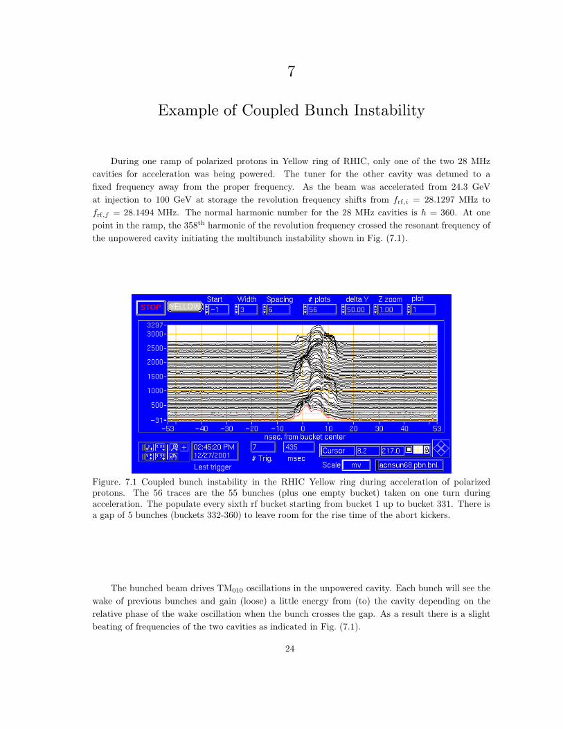
the unpowered cavity initiating the multibunch instability shown in Fig. (7.1).
Figure. 7.1 Coupled bunch instability in the RHIC Yellow ring during acceleration of polarizedprotons. The 56 traces are the 55 bunches (plus one empty bucket) taken on one turn duringacceleration. The populate every sixth rf bucket starting from bucket 1 up to bucket 331. There isa gap of 5 bunches (buckets 332-360) to leave room for the rise time of the abort kickers.
The bunched beam drives TM010 oscillations in the unpowered cavity. Each bunch will see the
wake of previous bunches and gain (loose) a little energy from (to) the cavity depending on the
relative phase of the wake oscillation when the bunch crosses the gap. As a result there is a slight
beating of frequencies of the two cavities as indicated in Fig. (7.1).
24

Example of Coupled Bunch Instability 25
-1-0.8-0.6-0.4-0.2
00.20.40.60.8
1
0 0.2 0.4 0.6 0.8 1
-1-0.8-0.6-0.4-0.2
00.20.40.60.8
1
Figure. 7.2Conceptual beating of the frequencies of the two cavities: [sin(2πhx) sin(2πh′x)]. Here
the harmonic numbers h = 20 [sin(2πhx)] and h′ = 18 [0.5 sin(2πh′x)] were used rather than 360
and 358, so that the individual cycles could be seen for the individual cavities.
This shows the 55 bunches later in the acceleration ramp after the oscillations have Landau damped.