Study of Electrode Kinetics
A thesis submitted for the degree of
Doctor of Philosophy
in Physical and Theoretical Chemistry
Danlei Li
Exeter College
Trinity Term 2020
Contents
Abstract ........................................................................................................................... x
Acknowledgements ........................................................................................................ xi
Glossary ......................................................................................................................... xii
Chapter 1 ......................................................................................................................... 1
Introduction to Electrochemistry .................................................................................. 1
1.1 Electrochemical equilibrium............................................................................... 2
1.2 Electrode kinetics in aqueous solution ............................................................. 10
1.2.1 Electrochemical cells ............................................................................. 10
1.2.2 Butler-Volmer (BV) kinetics for a simple one-electron transfer process
........................................................................................................................ 13
1.2.3 Tafel analysis ......................................................................................... 16
1.3 Mass transfer in electrochemical systems ........................................................ 18
1.3.1 Introduction of modes of mass transport ............................................... 18
1.3.2 Diffusion of species in solution ............................................................. 20
1.4 Electrochemical techniques: cyclic voltammetry ............................................. 26
1.4.1 Reversibility: mass transport versus electrode kinetics ......................... 27

1.4.2 Cyclic voltammetry at different electrode geometries .......................... 28
References: ............................................................................................................. 38
Chapter 2 ....................................................................................................................... 40
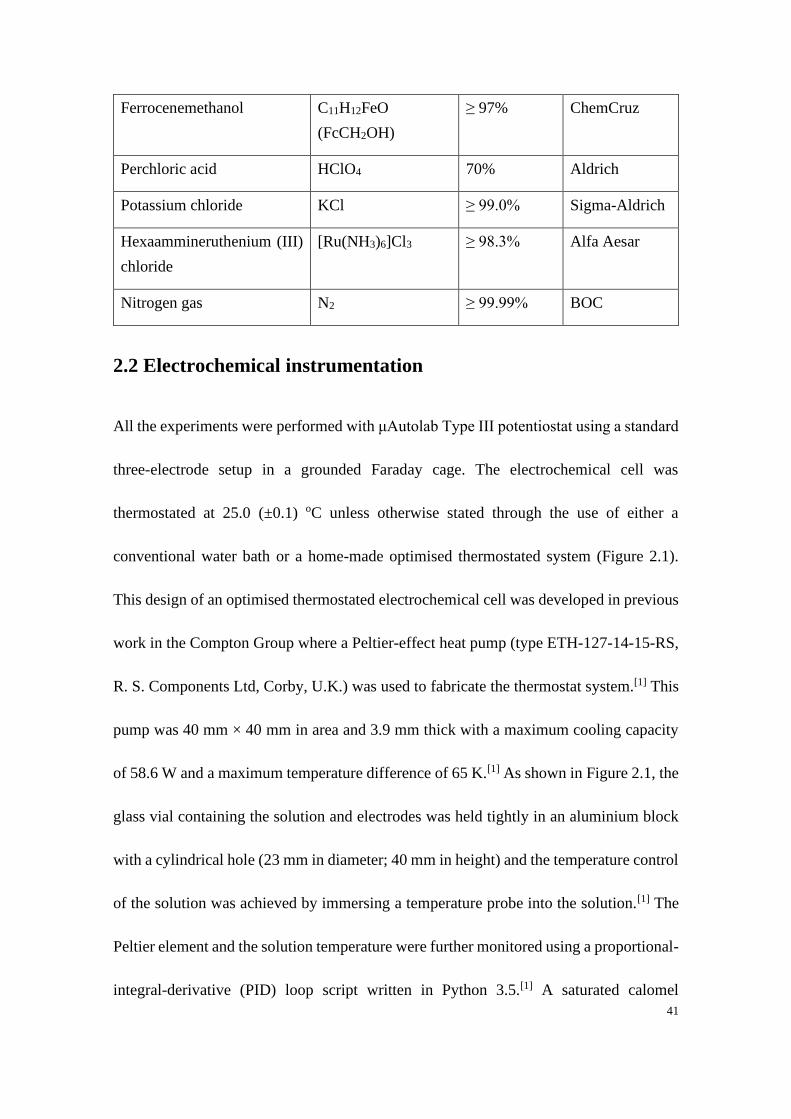
Experimental ................................................................................................................. 40
2.1 Chemical reagents............................................................................................. 40
2.2 Electrochemical instrumentation ...................................................................... 41
2.3 Preparation and geometries of the working electrodes ..................................... 43
2.3.1 Preparation of the working electrodes ................................................... 43
2.3.2 Geometries of the working electrodes ................................................... 44
2.4 Simulation programmes .................................................................................... 45
References: ............................................................................................................. 46
Chapter 3 ....................................................................................................................... 47
Voltammetric Demonstration of Thermally Induced Natural Convection in Aqueous
Solution .......................................................................................................................... 47
3.1 Introduction ...................................................................................................... 48
3.2 Experimental ..................................................................................................... 51
3.2.1 Chemical reagents.................................................................................. 51

3.2.2 Instrumentation ...................................................................................... 51
3.2.3 Electrochemical cell designs for the study of convection effect on
electrodes with different geometries............................................................... 52
3.2.4 Electrochemical cell design for the study of convective effects on a
macroelectrode with different orientations ..................................................... 55
3.2.5 Electrochemical measurements ............................................................. 56
3.3 Results and discussion ...................................................................................... 56
3.3.1 Chronoamperometric responses on a macrodisc electrode.................... 57
3.3.2 Evaporation effects on the voltammetric behaviour of a microcylinder
electrode.......................................................................................................... 62
3.3.3 Vibration effects on the voltammetric behaviour of a microcylinder
electrode.......................................................................................................... 65
3.3.4 Effect of natural convection on different electrode geometries ............ 70
3.4 Conclusions ...................................................................................................... 75
References: ............................................................................................................. 76
Chapter 4 ....................................................................................................................... 78
Tafel Analysis under Different Electrode Geometries .............................................. 78
4.1 Introduction ...................................................................................................... 79
4.2 Background theory ........................................................................................... 82
4.2.1 Butler-Volmer kinetics .......................................................................... 82
4.2.2 Tafel analysis ......................................................................................... 83
4.2.3 Mass-transport corrected Tafel analysis ................................................ 86
4.3 Numerical simulation procedures ..................................................................... 87
4.4 Results and discussion ...................................................................................... 91
4.4.1 Electrodes with linear diffusion ............................................................. 92
4.4.2 Microelectrodes under steady-state conditions ..................................... 99
4.4.3 Electrodes under quasi-steady state conditions ................................... 107
4.5 Conclusions .................................................................................................... 119
References: ........................................................................................................... 120
Chapter 5 ..................................................................................................................... 122
Some Thoughts About Reporting the Electrocatalytic Performance of
Nanomaterials ............................................................................................................. 122
5.1 Standard, formal and equilibrium potentials .................................................. 123
5.2 How should we quantify electrode-kinetics?.................................................. 125
5.3 What is an overpotential? ............................................................................... 129
5.4 What is an onset potential? ............................................................................. 132
5.5 What is the appropriate Tafel region of the current-potential plot of a half-cell
reaction in which to analyse a ‘Tafel slope’? ....................................................... 135
5.6 Units and electrochemical surface areas ......................................................... 138
5.7 Conclusions .................................................................................................... 141
References: ........................................................................................................... 141
Chapter 6 ..................................................................................................................... 143
Electrochemical Measurement of the Size of Microband Electrodes: A Theoretical
Study ............................................................................................................................ 143
6.1 Introduction .................................................................................................... 144
6.1.1 Background overview .......................................................................... 144
6.1.2 Fabrication methods ............................................................................ 147
6.2 Background theory ......................................................................................... 152
6.2.1 General theory background on band electrodes .................................. 152
6.2.2 Numerical simulation procedures ........................................................ 159
6.3 Results and discussion .................................................................................... 162
6.3.1 Fully reversible redox couple with equal diffusion coefficients ......... 163

6.3.2 Fully irreversible redox couple with equal diffusion coefficients ....... 165
6.3.3 Fully irreversible redox couple with unequal diffusion coefficients ... 173
6.3.4 Blind tests ............................................................................................ 180
6.4 Conclusions .................................................................................................... 187
References: ........................................................................................................... 188
Chapter 7 ..................................................................................................................... 190
Electrocatalysis via Intrinsic Surface Quinones Mediating Electron Transfer to and
from Carbon Electrodes ............................................................................................. 190
7.1 Introduction .................................................................................................... 191
7.2 Experimental ................................................................................................... 193
7.2.1 Chemical reagents................................................................................ 193
7.2.2 Instrumentation .................................................................................... 193
7.2.3 Electrochemical measurements ........................................................... 194
7.2.4 Simulation programmes ....................................................................... 195
7.3 Tafel analysis on a microdisc electrode .......................................................... 195
7.3.1 Mass-transport corrected transfer coefficient plots ............................. 196
7.3.2 Non-uniformly mass-transport corrected transfer coefficient plots .... 197
7.4 Results and discussion .................................................................................... 199
7.4.1 Determination of the diffusion coefficients and the formal potential of the
Fe2+/Fe3+ redox couple .................................................................................. 199
7.4.2 Comparison of voltammetric responses on gold and carbon microdisc
electrodes ...................................................................................................... 202
7.4.3 Transfer coefficient plots measured at carbon electrodes ................... 204
7.4.4 Adsorption of Fe2+/Fe3+ on a carbon microdisc electrode ................... 208
7.4.5 Proposed mechanistic model of the Fe2+/3+ redox process .................. 221
7.5 Conclusions .................................................................................................... 224
References: ........................................................................................................... 225
Chapter 8 ..................................................................................................................... 227
Mass Transport Corrected Transfer Coefficients from Microdisc Cyclic
Voltammetry: 2D Simulation and Experiment ........................................................ 227
8.1 Introduction .................................................................................................... 228
8.2 Applications of the Koutecky-Levich method and the normal mass transport
corrected method on a microdisc electrode .......................................................... 237
8.2.1 The Koutecky-Levich method on a microdisc electrode ..................... 237
8.2.2 The mass transport corrected method applied to a microdisc electrode
...................................................................................................................... 241
8.3 Experimental ................................................................................................... 246
8.3.1 Chemical reagents................................................................................ 246
8.3.2 Instrumentation .................................................................................... 246
8.4 Theory ............................................................................................................. 246
8.5 Numerical methods ......................................................................................... 251
8.6 Results and discussion .................................................................................... 252
8.6.1 Data extraction process ........................................................................ 252
8.6.2 Accuracy of the data extraction method .............................................. 254
8.6.3 Experimental example using the extraction method............................ 257
8.7 Conclusions .................................................................................................... 260
References: ........................................................................................................... 261
Chapter 9 ..................................................................................................................... 264
Overall Conclusions .................................................................................................... 264
Appendix A .................................................................................................................. 268
Section A1: Derivation of the analytical expression for the mass-transport corrected
transfer coefficient 𝜶′ in Chapter 4 ..................................................................... 268
Section A2: Establishing the lower current limit on different electrodes in Chapter 4
.............................................................................................................................. 271
Section A3: Determination for diffusion limit in Chapter 4 ................................. 273
References: ........................................................................................................... 274
Appendix B .................................................................................................................. 275
Section B1: Convergence test for the home-written microband programme ....... 275
Section B2: Blind tests ......................................................................................... 276
Section B2.1: Test 3 - Redox couple with low unequal diffusion coefficients (αa
= 0.3, αc = 0.7) .............................................................................................. 276
Section B2.2: Test 4 - Redox couple with low unequal diffusion coefficients (αa
= 0.4, αc = 0.6) .............................................................................................. 279
x
Study of Electrode Kinetics
Danlei Li
Exeter College, University of Oxford
A thesis submitted for the degree of D.Phil. in Physical and Theoretical Chemistry
Trinity Term, 2020
Abstract
This thesis reports the use of Tafel analysis in the study of electrode kinetics from both
theoretical and experimental perspectives.
During electrochemical measurements, any changes in temperature cause changes in
diffusion coefficient of the species, the electrochemical rate constant and the equilibrium
potential. Concequently, the improtance of temperature control in electrochemical
systems is first investigated. When and how thermally induced convective flows in bulk
solution influence the votlammetric behaviour are presented in Chapter 3.
Chapters 4 and 5 theoretically discuss what fraction of a voltammetric wave is appropriate
to use as the Tafel region for accurate analysis under linear, quasi-steady-state and steady-
state mass-transport regimes for an irreversible one-electron transfer process. The
measured transfer coefficient is found to deviate significantly from its true value as a
function of potential due to the mass-transport limitation at high overpotentials. If and
how a simple analytical mass-transport correction using a plot of ln |1
𝐼−
1
𝐼𝑙𝑖𝑚| against
potential can be used to improve the measurement of transfer coefficient is investigated.
The methodology of measuring transfer coefficient is further employed in the
electrochemical characterisation of a single microband electrode with unknown
dimensions (Chapter 6). Such Tafel analysis is applied to an experimental study where
the intrinsic surface quinones on carbon substrates can catalyse Fe2+/3+ redox reaction
evidenced by a potential dependent transfer coefficient (Chapter 7).
Last but not least, a new simulation techinique is developed in Chapter 8 to extract the
kinetic information from experimental voltammograms for electrodes under both radial
and liner regimes on the basis of the prior knowledge of the physical parameters defining
the system, most importantly the diffusion coefficient, analyte concentration and
electrode radius.
xi
Acknowledgements
First of all, I would like to express great thanks to my supervisor, Professor Richard
Compton, for all the invaluable support and guidance throughout my D.Phil. study. Thank
you for providing me lots of opportunities to develop my scientific skills as well as
knowledge. Your meticulous attitude and passion about the research always inspired me
during my D.Phil. I am now becoming more positive and thoughtful towards the
difficulties.
Second, my deep appreciation goes to Dr Christopher Batchelor-McAuley for your
generous help and constructive advice which have made a significant contribution
towards my D.Phil. You are always so supportive and patient when I was in trouble. I
could learn some new knowledge from every single discussion with you. My D.Phil.
would not have been so productive without your help. I also would like to acknowledge
Lifu who was such a helpful senior group member and friend. My D.Phil. would not have
started smoothly without your help and guidance of the experiments when I was a totally
‘fresher’ to the group. Thanks to Dr Chuhong Lin for the home-written programme which
has been employed throughout my projects.
To Jake, Ruochen and Haonan, it has been lucky for me to have you preparing and
achieving milestones of the D.Phil. together. To Archana, Yuanyuan and Yifei, I would
be more than happy if I have ever helped you in some ways during your research. To
Yuanzhe, Haotian, Bertold, Xiuting and many other group members of the past and
present, I have been truly enjoying working with you. I felt so lucky to have the chance
to be a member of such a wonderful group full of warmth, kindness and experitise. I am
also greatful to the funding from China Scholarship Council and University of Oxford.
Special thanks to my ‘Oxford Family’ -Xin and Yanjun- who were and are so considerate
in many ways. It has been so nice to have you two as housemates. The tasty food I
received from you, especially Xin, have given me lots of happiness and energy. Thank
you for taking care of me and always being my side. Special thanks to my “Pigeon”
friends for the uncountable joy and ease you brought to me during the pandemic.
Last but not least, I would like to express heartfelt thanks to my parents and other family
members for your deepest love, strongest support and constant encouragement. I could
be so brave and positive is because I know you are always there. Undertaking this D.Phil.
has been a meaningful and valuable experience in my life. It would not be possible for
me to complete D.Phil. without the help and support from all of you.

xii
Glossary
Roman Symbols
Symbol Meaning Units
𝑨 (a) area
(b) frequency factor in a rate expression (1st order)
(c) oxidised form of the system 𝐴 + 𝑒− ⇌ 𝐵
cm2
s-1
none
𝒂𝒊 Activity of species 𝑖 none
𝒃 Tafel slope mV dec-1
𝑩 Reduced form of the system 𝐴 + 𝑒− ⇌ 𝐵 none
𝑪𝒅𝒍 Capacitance of the double layer F cm-2
𝒄𝒊,𝒃𝒖𝒍𝒌 Bulk concentration of species 𝑖 mol dm-3
𝒄𝒊,𝟎 Concentration of species 𝑖 at the electrode surface mol dm-3
𝒄⦵ Standard concentration (1 mol dm-3) mol dm-3
𝑫𝒊 Diffusion coefficient of species 𝑖 m2 s-1
𝑫∞ Diffusion coefficient of species 𝑖 at infinite temperature m2 s-1
𝑬𝒂 Activation energy of a reaction kJ mol-1
𝑬 Applied potential at the electrode V
𝑬𝒑𝒂 Anodic peak potential V
𝑬𝒑𝒄 Cathodic peak potential V
𝑬𝒎𝒊𝒅 Mid-point potential V
𝑬𝒈 Energy gap V
xiii
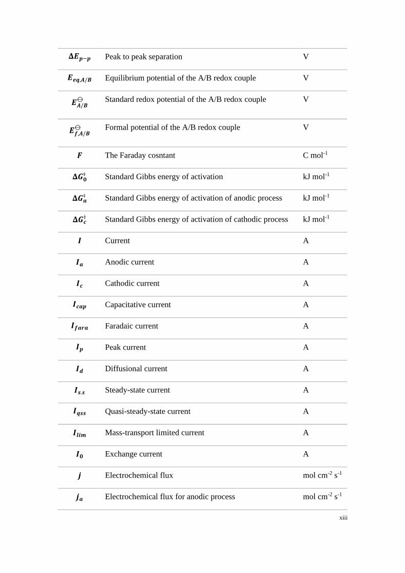
𝚫𝑬𝒑−𝒑 Peak to peak separation V
𝑬𝒆𝒒,𝑨/𝑩 Equilibrium potential of the A/B redox couple V
𝑬𝑨/𝑩⦵
Standard redox potential of the A/B redox couple V
𝑬𝒇,𝑨/𝑩⦵
Formal potential of the A/B redox couple V
𝑭 The Faraday cosntant C mol-1
𝚫𝑮𝟎‡ Standard Gibbs energy of activation kJ mol-1
𝚫𝑮𝒂‡ Standard Gibbs energy of activation of anodic process kJ mol-1
𝚫𝑮𝒄‡ Standard Gibbs energy of activation of cathodic process kJ mol-1
𝑰 Current A
𝑰𝒂 Anodic current A
𝑰𝒄 Cathodic current A
𝑰𝒄𝒂𝒑 Capacitative current A
𝑰𝒇𝒂𝒓𝒂 Faradaic current A
𝑰𝒑 Peak current A
𝑰𝒅 Diffusional current A
𝑰𝒔.𝒔 Steady-state current A
𝑰𝒒𝒔𝒔 Quasi-steady-state current A
𝑰𝒍𝒊𝒎 Mass-transport limited current A
𝑰𝟎 Exchange current A
𝒋 Electrochemical flux mol cm-2 s-1
𝒋𝒂 Electrochemical flux for anodic process mol cm-2 s-1
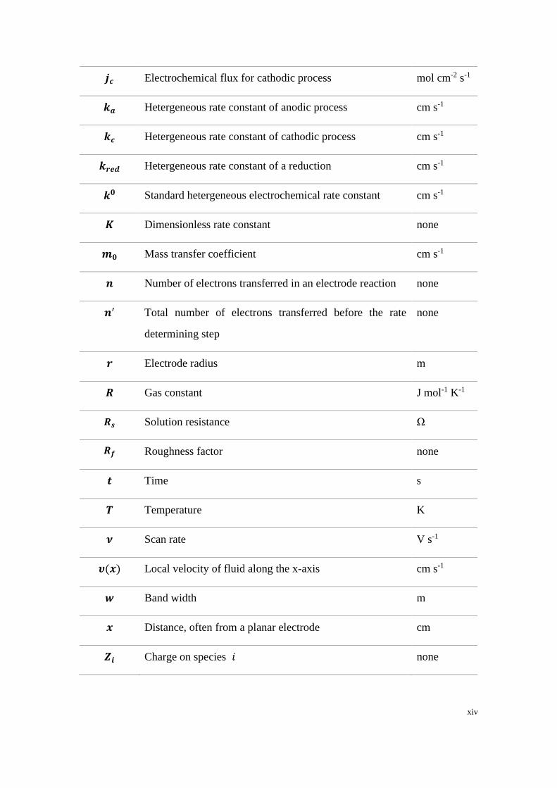
xiv
𝒋𝒄 Electrochemical flux for cathodic process mol cm-2 s-1
𝒌𝒂 Hetergeneous rate constant of anodic process cm s-1
𝒌𝒄 Hetergeneous rate constant of cathodic process cm s-1
𝒌𝒓𝒆𝒅 Hetergeneous rate constant of a reduction cm s-1
𝒌𝟎 Standard hetergeneous electrochemical rate constant cm s-1
𝑲 Dimensionless rate constant none
𝒎𝟎 Mass transfer coefficient cm s-1
𝒏 Number of electrons transferred in an electrode reaction none
𝒏′ Total number of electrons transferred before the rate
determining step
none
𝒓 Electrode radius m
𝑹 Gas constant J mol-1 K-1
𝑹𝒔 Solution resistance Ω
𝑹𝒇 Roughness factor none
𝒕 Time s
𝑻 Temperature K
𝝂 Scan rate V s-1
𝝊(𝒙) Local velocity of fluid along the x-axis cm s-1
𝒘 Band width m
𝒙 Distance, often from a planar electrode cm
𝒁𝒊 Charge on species 𝑖 none
xv
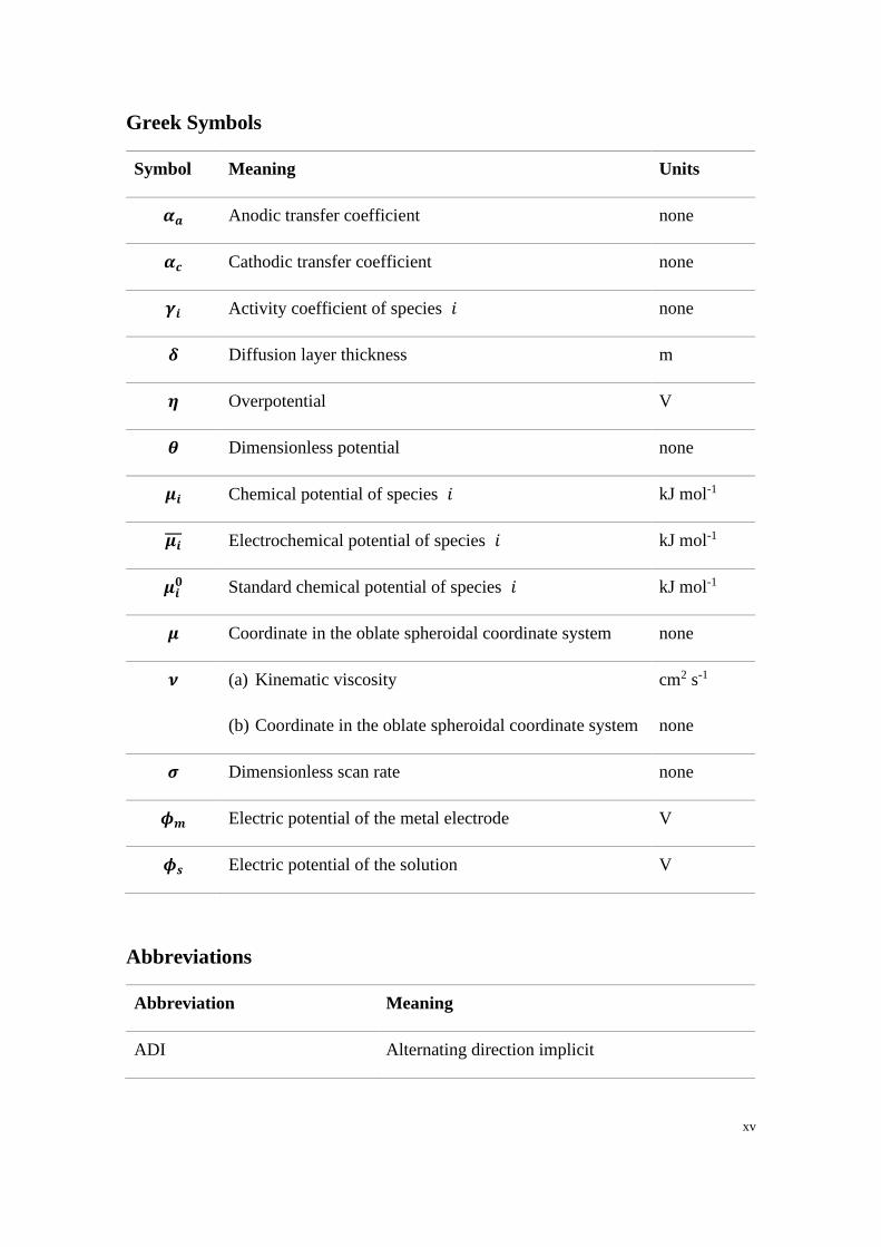
Greek Symbols
Symbol Meaning Units
𝜶𝒂 Anodic transfer coefficient none
𝜶𝒄 Cathodic transfer coefficient none
𝜸𝒊 Activity coefficient of species 𝑖 none
𝜹 Diffusion layer thickness m
𝜼 Overpotential V
𝜽 Dimensionless potential none
𝝁𝒊 Chemical potential of species 𝑖 kJ mol-1
𝝁𝒊 Electrochemical potential of species 𝑖 kJ mol-1
𝝁𝒊𝟎 Standard chemical potential of species 𝑖 kJ mol-1
𝝁 Coordinate in the oblate spheroidal coordinate system none
𝝂 (a) Kinematic viscosity
(b) Coordinate in the oblate spheroidal coordinate system
cm2 s-1
none
𝝈 Dimensionless scan rate none
𝝓𝒎 Electric potential of the metal electrode V
𝝓𝒔 Electric potential of the solution V
Abbreviations
Abbreviation Meaning
ADI Alternating direction implicit
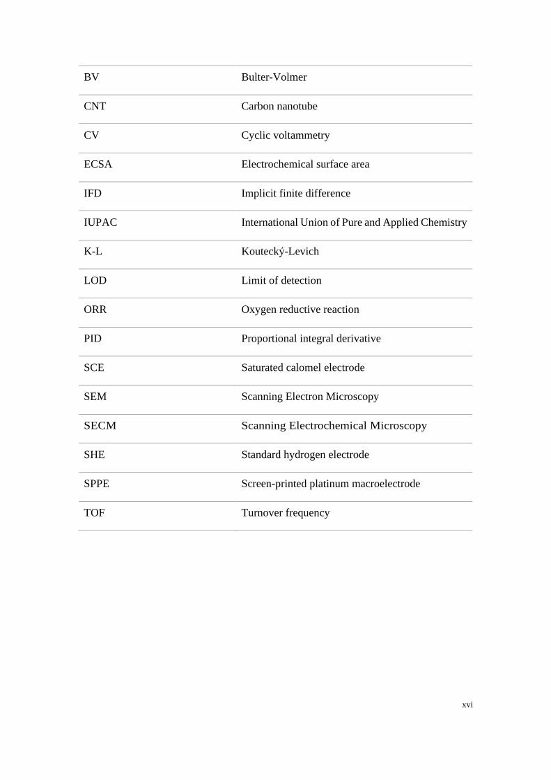
xvi
BV Bulter-Volmer
CNT Carbon nanotube
CV Cyclic voltammetry
ECSA Electrochemical surface area
IFD Implicit finite difference
IUPAC International Union of Pure and Applied Chemistry
K-L Koutecky-Levich
LOD Limit of detection
ORR Oxygen reductive reaction
PID Proportional integral derivative
SCE Saturated calomel electrode
SEM Scanning Electron Microscopy
SECM Scanning Electrochemical Microscopy
SHE Standard hydrogen electrode
SPPE Screen-printed platinum macroelectrode
TOF Turnover frequency
1
Chapter 1
Introduction to Electrochemistry
Electrochemistry is the important branch of chemistry which studies reactions involving
electron transfers, and which relates the flow of electrons to chemical changes. Such
reactions are called redox (reduction-oxidation) reactions. Electrochemical
measurements are powerful methods for studying the kinetics and thermodynamics of
such processes. Electrochemical processes are widely involved in daily life for instance
in metal corrosion and coating and the detection of breath alcohol in drivers through the
redox reaction of ethanol with dichromate[1]. In addition food sensors including chilli
sensors have been recently developed[2] along with the bio-electrochemical detection of
bacteria[3] and viruses[4]. Energy-related applications such as fuel cells and batteries (e.g.
lithium-ion batteries, all-vanadium redox flow batteries)[5] also provide significant
benefits to the world. Such research requires solid knowledge of fundamental
electrochemistry in order to have a better understanding of the science behind the redox
reactions. In this chapter, we give an overview of the fundamental principles of electrode
reactions as well as the electrochemical techniques used in this thesis, with the aim of
providing a clear background knowledge for the following chapters.
2
1.1 Electrochemical equilibrium
Electrochemistry studies the chemical processes involving electrons transfer across the
interface between an electronic conductor (an electrode) and an ionic conductor (an
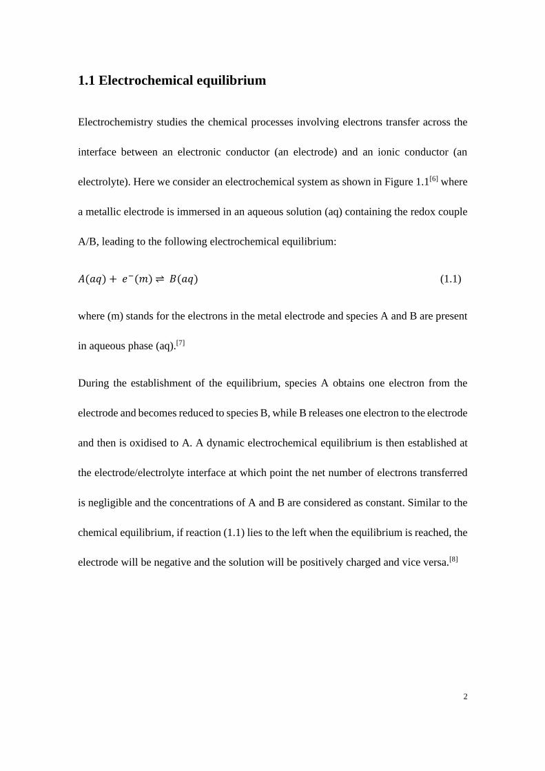
electrolyte). Here we consider an electrochemical system as shown in Figure 1.1[6] where
a metallic electrode is immersed in an aqueous solution (aq) containing the redox couple
A/B, leading to the following electrochemical equilibrium:
𝐴(𝑎𝑞) + 𝑒−(𝑚) ⇌ 𝐵(𝑎𝑞) (1.1)
where (m) stands for the electrons in the metal electrode and species A and B are present
in aqueous phase (aq).[7]
During the establishment of the equilibrium, species A obtains one electron from the
electrode and becomes reduced to species B, while B releases one electron to the electrode
and then is oxidised to A. A dynamic electrochemical equilibrium is then established at
the electrode/electrolyte interface at which point the net number of electrons transferred
is negligible and the concentrations of A and B are considered as constant. Similar to the
chemical equilibrium, if reaction (1.1) lies to the left when the equilibrium is reached, the
electrode will be negative and the solution will be positively charged and vice versa.[8]
3
Figure 1.1 A metallic electrode immersed into an aqueous solution containing an A/B redox couple.
The charge transfer induces a charge separation between the electrolyte and the electrode,
resulting in an electrical potential difference between them. An electrode potential is
therefore established at the electrode relative to the bulk solution. The resulting electrode
potential is associated with the energy levels of the species involved during the
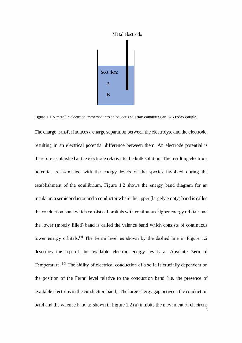
establishment of the equilibrium. Figure 1.2 shows the energy band diagram for an
insulator, a semiconductor and a conductor where the upper (largely empty) band is called
the conduction band which consists of orbitals with continuous higher energy orbitals and
the lower (mostly filled) band is called the valence band which consists of continuous
lower energy orbitals.[9] The Fermi level as shown by the dashed line in Figure 1.2
describes the top of the available electron energy levels at Absolute Zero of
Temperature.[10] The ability of electrical conduction of a solid is crucially dependent on
the position of the Fermi level relative to the conduction band (i.e. the presence of
available electrons in the conduction band). The large energy gap between the conduction
band and the valence band as shown in Figure 1.2 (a) inhibits the movement of electrons
4
from the valence band to the conduction band, resulting in an insulating characteristic
without electrical conductivity. The relatively small energy gap in semiconductor (Figure
1.2 b) provides possibility of electron conduction; electrons in the valence band can be
thermally excited to reach the conduction band and extra charge carriers can be added by
doping.[9] According to the energy diagram of a hypothetical metal shown in Figure 1.2(c),
the overlap of the conduction band and the valence band and existence of freely available
electrons provide easy electron conduction.[9]
Figure 1.2 Possible energy band diagrams for (a) insulator, (b) semiconductor and (c) metal. Eg stands for
the energy gap between the conduction band and the valence band. The dashed line represents the Fermi
level.
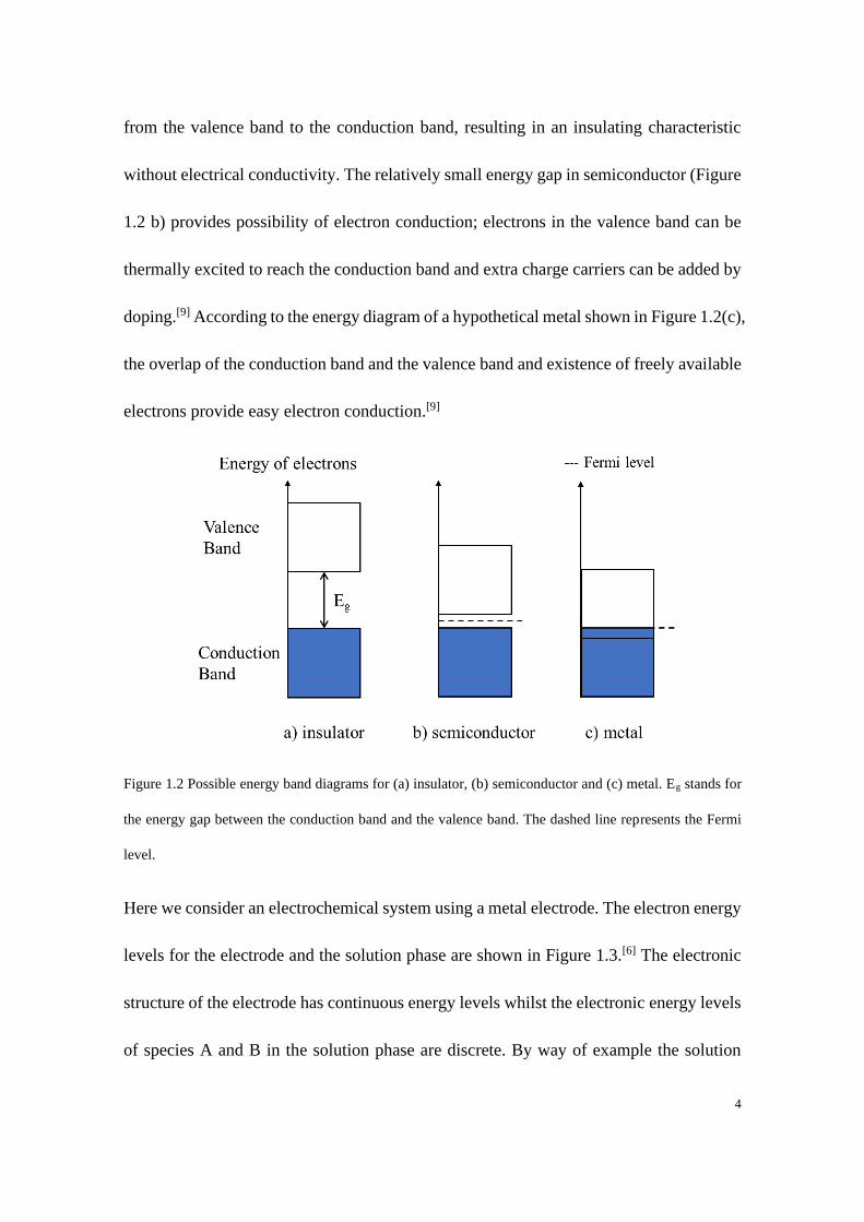
Here we consider an electrochemical system using a metal electrode. The electron energy
levels for the electrode and the solution phase are shown in Figure 1.3.[6] The electronic
structure of the electrode has continuous energy levels whilst the electronic energy levels
of species A and B in the solution phase are discrete. By way of example the solution
5
levels are assumed lower in energy than the Fermi Level of the electrode; in this case how
the energy of electrons changes before (a) and after (b) electron transfer at the
electrode/electrolyte interface is illustrated in Figure 1.3. The Fermi levels of the
electrode and the solution are not usually equal when an initially uncharged metal
electrode is immersed in an uncharged solution. In this example, before the electron
transfers it is energetically favourable for the electrons flowing from the metal with a
higher Fermi level to the vacant electronic states on species A in the solution phase and
gets reduced to B. The metallic electrode consequently becomes positively charged after
donating electrons to the ions which lowers the electronic energy presented as the lowered
Fermi level in Figure 1.3(b). Meanwhile the solution phase becomes negatively charged
and the electronic energy levels of the ions in the solution phase are progressively raised.
The dynamic equilibrium will be finally attained once the rates of the oxidation of B and
the reduction of A are the same (i.e. the rates of donating electrons to species A and
gaining electrons from species B are matched). Note that it is shown in Figure 1.3(b), a
charge separation due to the electron flowing exists between the metal electrode and the
solution phase when the equilibrium is attained, which is the origin of the electrode
potential established on the metal.[6] Of course if the Fermi level is below the solution
energy levels then electrons move into the electrode before equilibrium is reached and in
that case the electrode develops a negative charge.
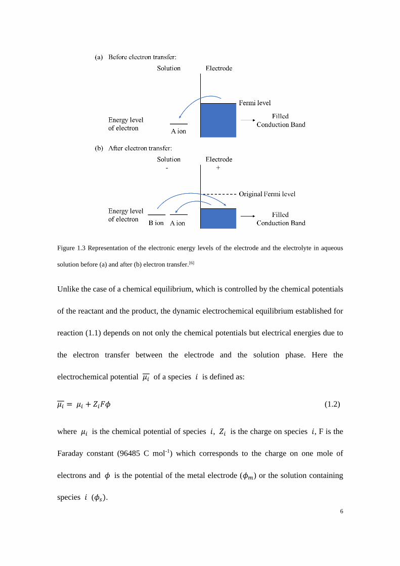
6
Figure 1.3 Representation of the electronic energy levels of the electrode and the electrolyte in aqueous
solution before (a) and after (b) electron transfer.[6]
Unlike the case of a chemical equilibrium, which is controlled by the chemical potentials
of the reactant and the product, the dynamic electrochemical equilibrium established for
reaction (1.1) depends on not only the chemical potentials but electrical energies due to
the electron transfer between the electrode and the solution phase. Here the
electrochemical potential 𝜇𝑖 of a species 𝑖 is defined as:
𝜇𝑖 = 𝜇𝑖 + 𝑍𝑖𝐹𝜙 (1.2)
where 𝜇𝑖 is the chemical potential of species 𝑖, 𝑍𝑖 is the charge on species 𝑖, F is the
Faraday constant (96485 C mol-1) which corresponds to the charge on one mole of
electrons and 𝜙 is the potential of the metal electrode (𝜙𝑚) or the solution containing
species 𝑖 (𝜙𝑠).

7
The chemical potential 𝜇𝑖 of species 𝑖 is defined as:
𝜇𝑖 = 𝜇𝑖0 + 𝑅𝑇𝑙𝑛𝑎𝑖 (1.3)
where 𝜇𝑖0 is the standard chemical potential of species 𝑖, R is the universal gas constant
(8.314 J K-1 mol-1), T is the temperature in K and 𝑎𝑖 is the activity of species 𝑖 in the
solution phase.
For reaction (1.1), the electrochemical potential at the equilibrium can be expressed as:
𝜇𝐴 + 𝜇𝑒− = 𝜇𝐵 (1.4)
Equation (1.4) can be converted to Equation (1.5) by applying Equation (1.2):
(𝜇𝐴 + 𝑍𝐴𝐹𝜙𝑠) + (𝜇𝑒− + 𝑍𝑒−𝐹𝜙𝑚) = 𝜇𝐵 + 𝑍𝐵𝐹𝜙𝑠 (1.5)
Considering the charge on electron is -1, hence
(𝜇𝐴 + 𝑍𝐴𝐹𝜙𝑠) + (𝜇𝑒− − 𝐹𝜙𝑚) = 𝜇𝐵 + (𝑍𝐴 − 1)𝐹𝜙𝑠 (1.6)
Rearranging Equation (1.6), we can get:
𝐹(𝜙𝑚 − 𝜙𝑠) = 𝜇𝐴 + 𝜇𝑒− − 𝜇𝐵 (1.7)
With the knowledge of the definition of chemical potential as shown in Equation (1.3),
Equation (1.7) can be written as:
𝜙𝑚 − 𝜙𝑠 =Δ𝜇0
𝐹+
𝑅𝑇
𝐹𝑙𝑛 (
𝑎𝐴
𝑎𝐵) (1.8)
8
where Δ𝜇0 = 𝜇𝐴0 + 𝜇𝑒− + 𝜇𝐵
0 which is a constant at a given temperature and pressure.
Equation (1.8) is known as one form of the Nernst Equation describing a single
electrode/solution interface in an electrochemical system as shown in Figure 1.1.
In reality the single boundary situation is extremely difficult to deal with as the potential
differences cannot be realistically measured; hence an electrochemical cell which consists
of two electrodes separated by at least one solution phase is necessarily employed. The
introduced second electrode is called a reference electrode and this ideally has a fixed
potential.[11] The internationally accepted primary reference electrode is the standard
hydrogen electrode (SHE) where the standard conditions have protons at unit activity and
hydrogen gas at one bar pressure. Other commonly used reference electrodes include the
saturated calomel electrode (SCE) of which the potential is 0.242 V versus SHE and the
silver-silver chloride electrode (Ag/AgCl) with a potential of 0.197 V in saturated KCl
versus SHE at 25 oC.[11-12] With the use of a reference electrode the measured potential
changes (ΔE) in the cell are all ascribable to the working electrode with respect to the
reference electrode as shown as Equation (1.9).
𝛥𝐸 = (𝜙𝑚 − 𝜙𝑠)𝑤𝑜𝑟𝑘𝑖𝑛𝑔 − (𝜙𝑚 − 𝜙𝑠)𝑟𝑒𝑓𝑒𝑟𝑒𝑛𝑐𝑒 (1.9)
The Nernst equation for the electrode potential in such a two-electrode system is then
expressed as:
𝐸 = 𝐸𝐴/𝐵⦵ +
𝑅𝑇
𝐹ln (
𝛼𝐴
𝛼𝐵) (1.10)
9
where 𝐸𝐴/𝐵⦵
is the standard redox potential of the A/B redox couple in the solution phase
measured against a SHE. However, due to the non-ideality of the solution, the
concentrations (𝑐𝑖) of the electroactive species are usually not equal to their activity (𝑎𝑖).
The relationship between the activities and the concentrations of the electroactive species
in solution phase has the expression 𝑎𝑖 = 𝛾𝑖𝑐𝑖/𝑐⦵, where 𝛾𝑖 is the activity coefficient
of species 𝑖 and 𝑐⦵ is the standard concentration (1 mol dm-3) we can write:
𝐸 = 𝐸𝐴/𝐵⦵ −
𝑅𝑇
𝐹𝑙𝑛
𝛾𝐵
𝛾𝐴−
𝑅𝑇
𝐹𝑙𝑛
𝑐𝐵
𝑐𝐴 (1.11)
The formal potential (𝐸𝑓,𝐴/𝐵⦵ ) of the A/B redox couple can then be expressed as:
𝐸𝑓,𝐴/𝐵⦵ = 𝐸𝐴/𝐵
⦵ −𝑅𝑇
𝐹𝑙𝑛
𝛾𝐵
𝛾𝐴 (1.12)
For a simple one-electron transfer process (reaction 1.1), the Nernst equation describing
the dynamic electrochemical equilibrium is consequently defined as:
𝐸𝑒𝑞,𝐴/𝐵 = 𝐸𝑓,𝐴/𝐵⦵ −
𝑅𝑇
𝐹𝑙𝑛
𝑐𝐵
𝑐𝐴 (1.13)
Note that Equation (1.13) is sensitive to the ratio of the concentrations of species A and
B. If a solution contains one order of magnitude higher concentration of the product as
compared to the reactant the equilibrium potential will be ~59.1 mV negative of the
formal potential of the system at 298K .[6] Classically the electrode potential is measured
using a potentiometer which requires fast electrode kinetics in order to establish the
dynamic electrochemical equilibrium as discussed in the next section.
10
1.2 Electrode kinetics in aqueous solution
1.2.1 Electrochemical cells
The two-electrode system mentioned above provides a feasible way to measure the
equilibrium electrode potential at a working electrode (albeit relative to a reference
electrode) which is expressed as Equation (1.9): Δ𝐸 = (𝜙𝑚 − 𝜙𝑠)𝑤𝑜𝑟𝑘𝑖𝑛𝑔 − (𝜙𝑚 −
𝜙𝑠)𝑟𝑒𝑓𝑒𝑟𝑒𝑛𝑐𝑒 where (𝜙𝑚 − 𝜙𝑠)𝑟𝑒𝑓𝑒𝑟𝑒𝑛𝑐𝑒 is assumed as a fixed value during the
measurements. In practical measurements away from equilibrium, as shown in Figure 1.4
(a), if a two electrode system is used when a potential is applied to the working electrode,
the generated current passes through both the working electrode and reference electrode,
resulting in chemical changes inside the reference electrode (and hence a change in its
potential). Moreover, a potential drop (𝑖𝑅𝑠), also known as ‘ohmic drop’, is gained due
to the resistance of the solution (𝑅𝑠) between the two electrodes. The potential, E, applied
between the two electrodes is then given by:
𝐸 = (𝜙𝑚 − 𝜙𝑠)𝑤𝑜𝑟𝑘𝑖𝑛𝑔 − (𝜙𝑚 − 𝜙𝑠)𝑟𝑒𝑓𝑒𝑟𝑒𝑛𝑐𝑒 + 𝑖𝑅𝑠 (1.14)
The first term on the right-hand side of Equation (1.14) relates to the driving force for the
electron transfer at the interface of interest and for a quantitative study changes in
potential need to be reflected directly in this term. This requires the second term
((𝜙𝑚 − 𝜙𝑠)𝑟𝑒𝑓𝑒𝑟𝑒𝑛𝑐𝑒) to be constant which in turn dictates that no current can pass through
the reference electrode as discussed above. In addition, the third term, 𝑖𝑅𝑠, needs to be

11
eliminated or minimised if changes in potential are to be reflected in changes in
(𝜙𝑚 − 𝜙𝑠)𝑤𝑜𝑟𝑘𝑖𝑛𝑔.
To minimise the two, unwanted contributions a third electrode called a counter electrode
(or auxiliary electrode) is consequently introduced to set up a three-electrode cell system
as shown in Figures 1.4 (b) and (c). A device called potentiostat is used to control the
electrochemical cell, which is able to impose a fixed potential between the working
electrode and reference electrode, which drives the redox reaction of interest generating
a current response. The current passes through the counter electrode but not the reference
electrode. This allows the generation of current-voltage response at the working
electrode/solution interface and the investigation of the redox reaction. To avoid the issue
of potential change raised in a two-electrode system due to the current flowing across the
reference electrode, the use of potentiostat which has a high impedance draws a negligible
current flow through the reference electrode. The same amount of current as that flowing
through the working electrode is then driven by the potentiostat to pass between the
working electrode and the counter electrode to complete the electric circuit. The potential
of the reference electrode ((𝜙𝑚 − 𝜙𝑠)𝑟𝑒𝑓𝑒𝑟𝑒𝑛𝑐𝑒) can then be considered as a fixed value
and also the unwanted contribution from the resistance between the working electrode
and the reference electrode is minimised. In such a three-electrode cell, all the changes in
the potential, E, appear in the term (𝜙𝑚 − 𝜙𝑠)𝑤𝑜𝑟𝑘𝑖𝑛𝑔 and the working electrode is
regarded as being ‘potentiostatted’. The counter electrode is chosen to have a good
12
electrical conductivity, a high surface area and not to produce any substances that affect
the reactions of interest.[13]
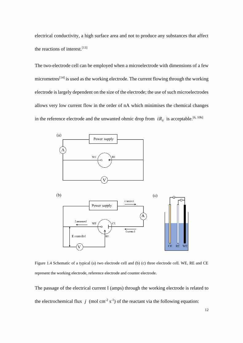
The two-electrode cell can be employed when a microelectrode with dimensions of a few
micrometres[14] is used as the working electrode. The current flowing through the working
electrode is largely dependent on the size of the electrode; the use of such microelectrodes
allows very low current flow in the order of nA which minimises the chemical changes
in the reference electrode and the unwanted ohmic drop from 𝑖𝑅𝑠 is acceptable.[6, 10b]
Figure 1.4 Schematic of a typical (a) two electrode cell and (b) (c) three electrode cell. WE, RE and CE
represent the working electrode, reference electrode and counter electrode.
The passage of the electrical current I (amps) through the working electrode is related to
the electrochemical flux 𝑗 (mol cm-2 s-1) of the reactant via the following equation:
13
𝐼 = −𝑛𝐹𝑗𝐴 (1.15)
where A the electrode area in cm2 and n=1 throughout the thesis for a one electron transfer
process. The electrochemical flux measures the rate of heterogeneous interfacial reaction,
which if assumed to be first order can be written as:
𝑗𝑎/𝑐 = 𝑘𝑎/𝑐[𝑟𝑒𝑎𝑐𝑡𝑎𝑛𝑡]0 (1.16)
where 𝑗𝑎/𝑐 is the electrochemical flux for anodic (oxidative) or cathodic (reductive)
reaction, 𝑘𝑎/𝑐 is the heterogeneous rate constant for anodic or cathodic reaction (cm s-1)
and subscript ‘0’ stands for the concentration of the reactant at the electrode surface. Note
that the concentration at the electrode surface [𝑟𝑒𝑎𝑐𝑡𝑎𝑛𝑡]0 is generally different from
that of the bulk solution [𝑟𝑒𝑎𝑐𝑡𝑎𝑛𝑡]𝑏𝑢𝑙𝑘 due to the mass transport of the species from
the bulk solution to the interface, which will be discussed later in this chapter.
1.2.2 Butler-Volmer (BV) kinetics for a simple one-electron transfer process
Here we consider a simple one-electron transfer process as discussed above in reaction
(1.1):
(1.17)
The total (net) flux can be expressed using the rate law as shown in Equation (1.16):
𝑗𝑡𝑜𝑡 = 𝑗𝑐 − 𝑗𝑎 = 𝑘𝑐[𝐴]0 − 𝑘𝑎[𝐵]0 (1.18)
14
According to Equation (1.18), the cathodic reaction will become dominant at relatively
negative overpotentials and the anodic reaction will dominate at relatively positive
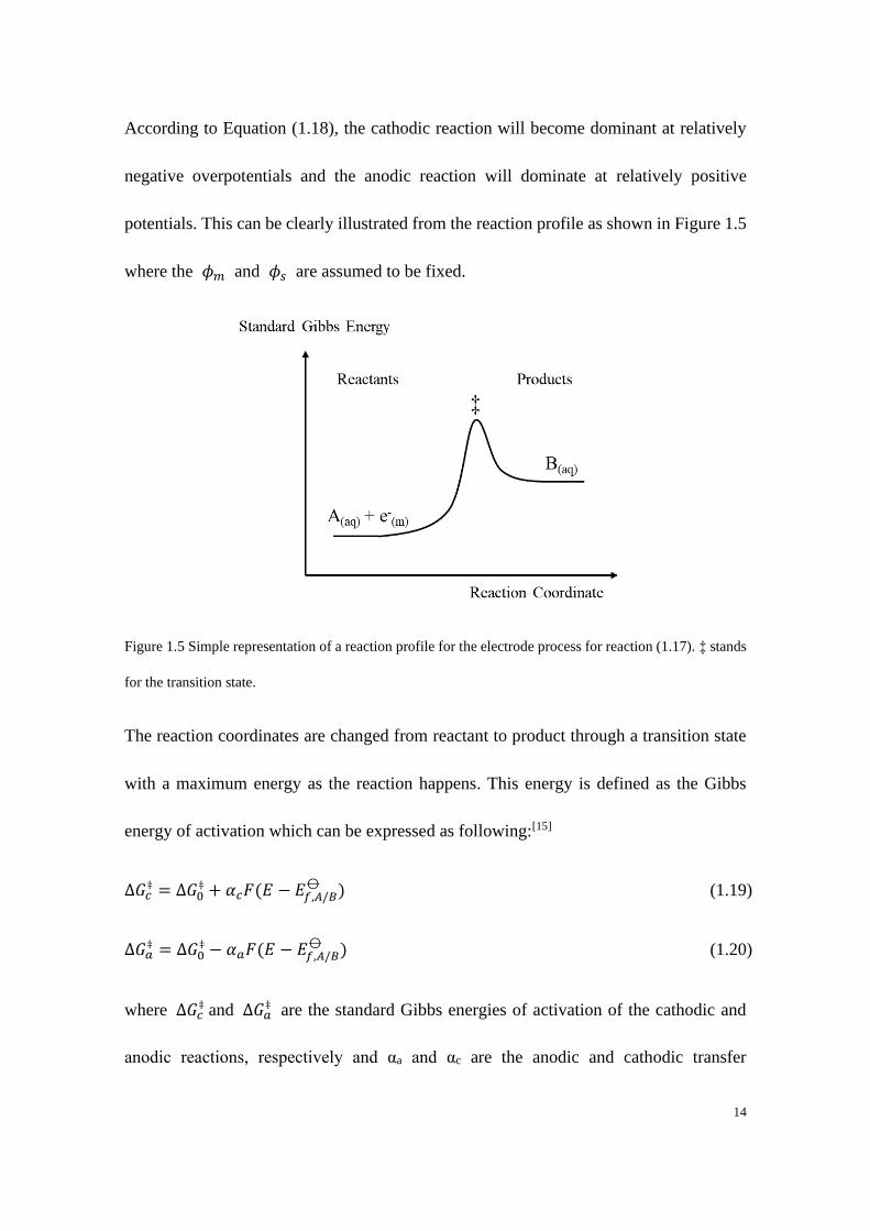
potentials. This can be clearly illustrated from the reaction profile as shown in Figure 1.5
where the 𝜙𝑚 and 𝜙𝑠 are assumed to be fixed.
Figure 1.5 Simple representation of a reaction profile for the electrode process for reaction (1.17). ‡ stands
for the transition state.
The reaction coordinates are changed from reactant to product through a transition state
with a maximum energy as the reaction happens. This energy is defined as the Gibbs
energy of activation which can be expressed as following:[15]
Δ𝐺𝑐‡ = Δ𝐺0
‡ + 𝛼𝑐𝐹(𝐸 − 𝐸𝑓,𝐴/𝐵⦵ ) (1.19)
Δ𝐺𝑎‡ = Δ𝐺0
‡ − 𝛼𝑎𝐹(𝐸 − 𝐸𝑓,𝐴/𝐵⦵ ) (1.20)
where Δ𝐺𝑐‡ and Δ𝐺𝑎
‡ are the standard Gibbs energies of activation of the cathodic and
anodic reactions, respectively and αa and αc are the anodic and cathodic transfer
15
coefficients of which the values are between 0 to 1. For a one-electrode transfer process
normally αa + αc =1.[16]
According to the Arrhenius Equation, the rate constants for cathodic and anodic processes
are given by[10b]:
𝑘𝑐 = 𝐴𝑐𝑒−Δ𝐺𝑐
‡
𝑅𝑇⁄
(1.21)
𝑘𝑎 = 𝐴𝑎𝑒−Δ𝐺𝑎
‡
𝑅𝑇⁄
(1.22)
where Aa/c is the exponential factor which is generally known as the frequency factor.
The existence of the temperature T implies the importance of temperature control during
electrochemical measurements.
Substituting Δ𝐺𝑐‡ and Δ𝐺𝑎
‡ in Equations (1.21) and (1.22) using Equations (1.19) and
(1.20):
𝑘𝑐 = 𝐴𝑐𝑒−Δ𝐺0
‡
𝑅𝑇⁄
× 𝑒−𝛼𝑐𝐹(𝐸−𝐸𝑓,𝐴/𝐵⦵ )/𝑅𝑇
(1.23)
𝑘𝑎 = 𝐴𝑎𝑒−Δ𝐺0
‡
𝑅𝑇⁄
× 𝑒𝛼𝑎𝐹(𝐸−𝐸𝑓,𝐴/𝐵⦵ )/𝑅𝑇
(1.24)
At the formal potential the anodic and cathodic rate constants become equal if the bulk
concentrations and A and B are the same, and equal to the standard electrochemical rate
constant:
𝑘0 = 𝑘𝑐 = 𝐴𝑐𝑒−Δ𝐺𝑐
‡
𝑅𝑇⁄
= 𝑘𝑎 = 𝐴𝑎𝑒−Δ𝐺𝑎
‡
𝑅𝑇⁄
(1.25)
The rate constants at other potentials can then be expressed as:
16
𝑘𝑐 = 𝑘0 × 𝑒−𝛼𝑐𝐹(𝐸−𝐸𝑓,𝐴/𝐵⦵ )/𝑅𝑇
(1.26)
𝑘𝑎 = 𝑘0 × 𝑒𝛼𝑎𝐹(𝐸−𝐸𝑓,𝐴/𝐵⦵ )/𝑅𝑇
(1.27)
Now the total net flux measured at the working electrode can be expressed as Equation
(1.28), which is known as the Butler-Volmer Equation.[17]
𝑗𝑡𝑜𝑡 = −𝐹𝑘𝐴/𝐵0 (c𝐴,0exp (
−𝛼𝑐𝐹
𝑅𝑇(𝐸 − 𝐸𝑓,𝐴/𝐵
⦵ )) − 𝑐𝐵,0exp (𝛼𝑎𝐹
𝑅𝑇(𝐸 − 𝐸𝑓,𝐴/𝐵
⦵ ))) (1.28)
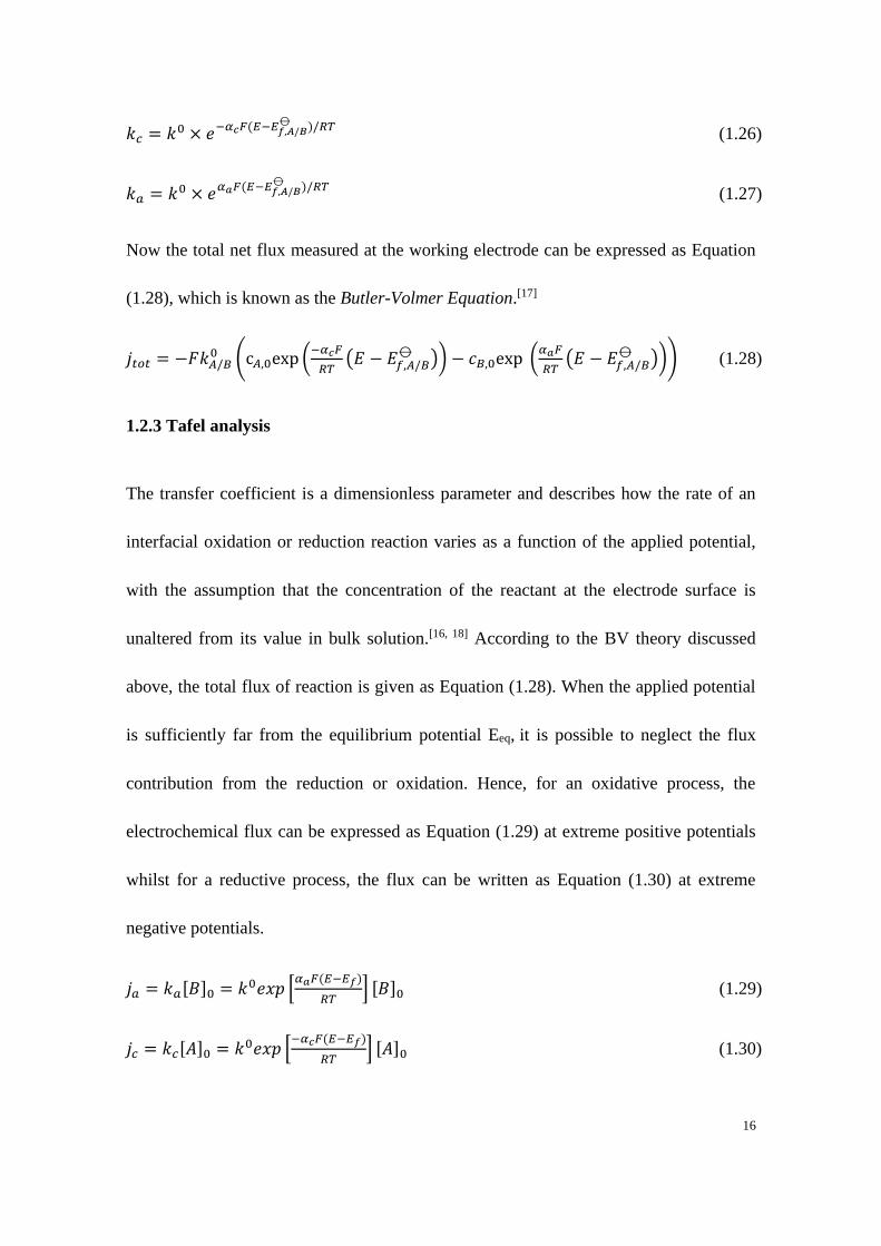
1.2.3 Tafel analysis
The transfer coefficient is a dimensionless parameter and describes how the rate of an
interfacial oxidation or reduction reaction varies as a function of the applied potential,
with the assumption that the concentration of the reactant at the electrode surface is
unaltered from its value in bulk solution.[16, 18] According to the BV theory discussed
above, the total flux of reaction is given as Equation (1.28). When the applied potential
is sufficiently far from the equilibrium potential Eeq, it is possible to neglect the flux
contribution from the reduction or oxidation. Hence, for an oxidative process, the
electrochemical flux can be expressed as Equation (1.29) at extreme positive potentials
whilst for a reductive process, the flux can be written as Equation (1.30) at extreme
negative potentials.
𝑗𝑎 = 𝑘𝑎[𝐵]0 = 𝑘0𝑒𝑥𝑝 [𝛼𝑎𝐹(𝐸−𝐸𝑓)
𝑅𝑇] [𝐵]0 (1.29)
𝑗𝑐 = 𝑘𝑐[𝐴]0 = 𝑘0𝑒𝑥𝑝 [−𝛼𝑐𝐹(𝐸−𝐸𝑓)
𝑅𝑇] [𝐴]0 (1.30)
17
Recall that the flux is related to the measured current using Equation 𝐼 = 𝐹𝑗𝐴. Equations
(1.29) and (1.30) can be rearranged as:
ln|𝐼𝑎| =𝛼𝑎𝐹(𝐸−𝐸𝑓
0)
𝑅𝑇+ 𝑙𝑛(𝐹𝐴𝑘0[𝐴]0) (1.31)
ln|𝐼𝑐| =−𝛼𝑐𝐹(𝐸−𝐸𝑓
0)
𝑅𝑇+ 𝑙𝑛(𝐹𝐴𝑘0[𝐴]0) (1.32)
Hence, if the concentration at the electrode surface is assumed constant with respect to its
bulk solution, a straight line with a gradient proportional to the transfer coefficient is
obtained by plotting ln|𝐼𝑎/𝑐| versus E as shown in Figure 1.6. For a one-electron transfer
process, 𝛼𝑎 + 𝛼𝑐 = 1 and the transfer coefficient is commonly qualitatively interpreted
as a measure of the ‘position’ of the transition state[19], where a transfer coefficient close
to zero implies the transition state is ‘reactant-like’ and similarly a value close to unity
implies a ‘product-like’ transition state for an reductive process.
Figure 1.6 Tafel plots for (a) reductive and (b) oxidative processes.
18
1.3 Mass transfer in electrochemical systems
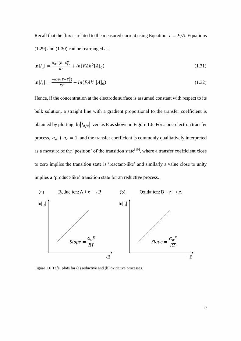
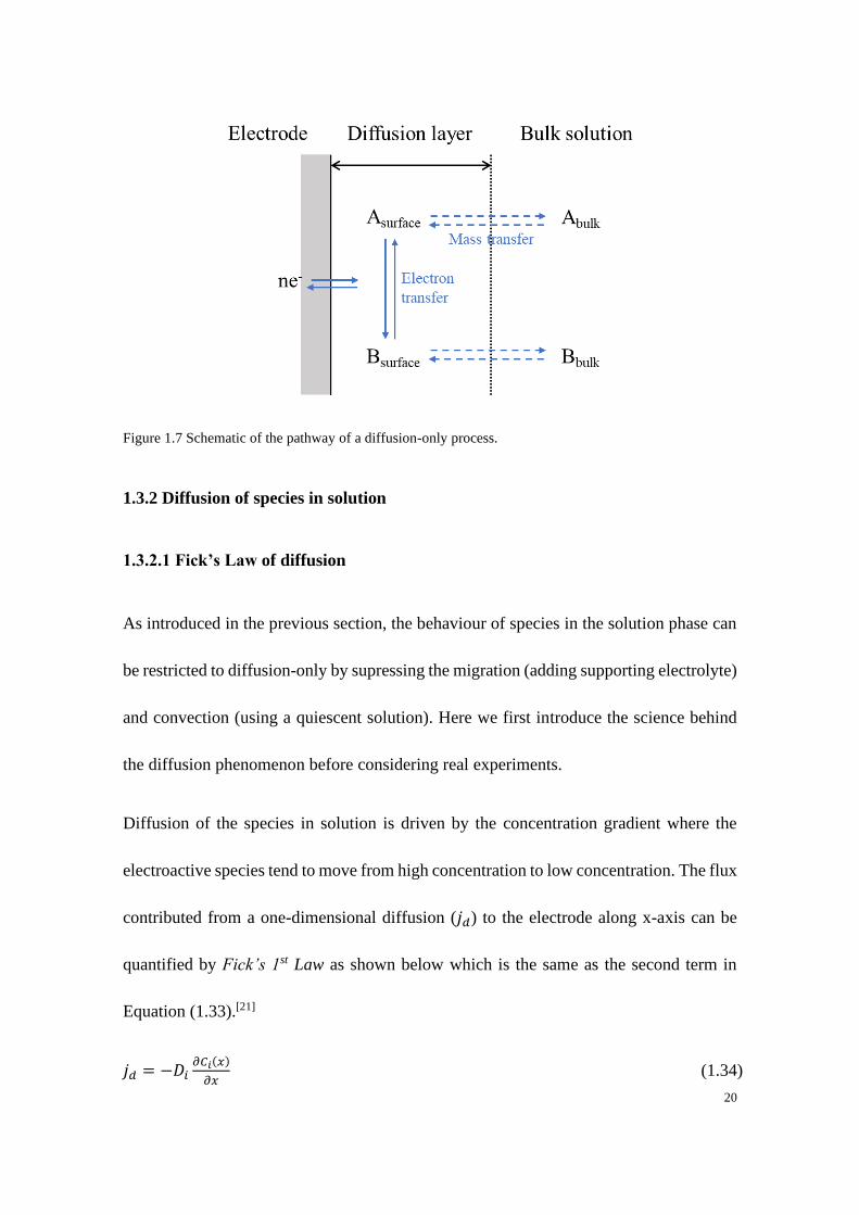
1.3.1 Introduction of modes of mass transport
Electrochemical mass transport is defined as the movement of the species in the bulk
solution to the reaction interface (i.e. the electrode/solution interface) as illustrated in
Figure 1.7. The reaction happens when the electroactive species is transferred to the
interface, therefore how the species transported to the electrode surface plays an important
role in studying the electrode kinetics. There are three modes of mass transport:[20]
a) Migration: this describes the movement of a charged molecule driven by the electrical
potential gradient (i.e. under an electric field).
b) Diffusion: this describes the movement of species driven by the concentration
gradient.
c) Convection: this describes the movement of species driven by the density gradient of
the species themselves (natural convection) or external forces such as stirring or
pumping (forced convection).
One-dimensional mass transport to an electrode along the x-axis is govern by the Nernst-
Planck equation:[10b]
𝑗𝑖(𝑥) = −𝑧𝑖𝐹
𝑅𝑇𝐷𝑖𝐶𝑖
𝜕𝜙(𝑥)
𝜕𝑥− 𝐷𝑖
𝜕𝐶𝑖(𝑥)
𝜕𝑥+ 𝐶𝑖𝜐(𝑥) (1.33)
19
where 𝑥 is the distance from the electrode surface (cm), 𝑗𝑖(𝑥) is the flux of species 𝑖
at distance x (mol cm-2 s-1), 𝐷𝑖 is the diffusion coefficient of species 𝑖 (cm2 s-1), 𝐶𝑖 is
the concentration of species 𝑖 (mol cm-3), 𝜕𝜙(𝑥)
𝜕𝑥 is the potential gradient,
𝜕𝐶𝑖(𝑥)
𝜕𝑥 is the
local concentration gradient at distance x, and 𝜐(𝑥) is the local velocity of fluid along
the axis (cm s-1). The three terms on the right stand for the flux contributions from
migration, diffusion and convection, respectively. The negative sign in the equation
implies the flux is down the gradient. The study of electrochemical systems with all the
three modes of mass transport involved is mathematically complicated. The system is
normally designed to eliminate one or two of the transport modes for the ease of
investigation. The migration effect can be supressed to negligible by adding a supporting
electrolyte (an inert electrolyte) with a much higher concentration (>100 times higher)
than that of the electroactive species. The addition of such supporting electrolyte also
decreases the solution resistance which improves the accuracy of the potential measured
or controlled at the working electrode. The convection effect can be eliminated by
avoiding the stirring and vibration of the solution and the possible density gradient
introduced due to the temperature difference which will be investigated in detail later in
Chapter 3. The diffusion of species in the solution is one of the key points in this thesis
which will be discussed further in the following sections.
20
Figure 1.7 Schematic of the pathway of a diffusion-only process.
1.3.2 Diffusion of species in solution
1.3.2.1 Fick’s Law of diffusion
As introduced in the previous section, the behaviour of species in the solution phase can
be restricted to diffusion-only by supressing the migration (adding supporting electrolyte)
and convection (using a quiescent solution). Here we first introduce the science behind
the diffusion phenomenon before considering real experiments.
Diffusion of the species in solution is driven by the concentration gradient where the
electroactive species tend to move from high concentration to low concentration. The flux
contributed from a one-dimensional diffusion (𝑗𝑑) to the electrode along x-axis can be
quantified by Fick’s 1st Law as shown below which is the same as the second term in
Equation (1.33).[21]
𝑗𝑑 = −𝐷𝑖𝜕𝐶𝑖(𝑥)
𝜕𝑥 (1.34)
21
It is known that in the same way that a rate constant is dependent on the temperature, the
diffusion coefficient of species 𝑖 is also strongly dependent on the temperature following
an Arrhenius type relationship:
𝐷𝑖 = 𝐷∞exp (−𝐸𝑎
𝑅𝑇) (1.35)
where 𝐷∞ is the diffusion coefficient of species 𝑖 at infinite temperature and 𝐸𝑎 is the
activation energy for diffusion. This relationship further implies the requirement of a high
quality thermostated system during electrochemical experiments.
Fick’s 1st Law provides information on how the flux and concentration of the species 𝑖
varies with the distance to the interface. The relationship between the flux and local
concentration of the species 𝑖 at the distance x and the time t is further given by Fick’s
2nd Law of diffusion, which is derived from Fick’s 1st Law by considering mass
conservation.
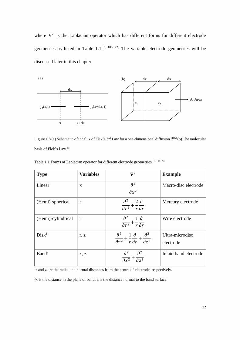
Now we consider a one-dimensional system as shown in Figure 1.8(a), according to
Fick’s 2nd Law, the change in concentration of species 𝑖 with time:
𝜕𝐶𝑖(𝑥,𝑡)
𝜕𝑡= 𝐷𝑖
𝜕𝐶𝑖(𝑥,𝑡)
𝜕𝑥2 (1.36)
The equation can be written as following in three-dimensions:
𝜕𝐶𝑖
𝜕𝑡= 𝐷𝑖∇
2𝐶𝑖 (1.37)
22
where ∇2 is the Laplacian operator which has different forms for different electrode
geometries as listed in Table 1.1.[6, 10b, 22] The variable electrode geometries will be
discussed later in this chapter.
Figure 1.8 (a) Schematic of the flux of Fick’s 2nd Law for a one-dimensional diffusion.[10b] (b) The molecular
basis of Fick’s Law.[6]
Table 1.1 Forms of Laplacian operator for different electrode geometries.[6, 10b, 22]
Type Variables 𝛁𝟐 Example
Linear x 𝜕2
𝜕𝑥2
Macro-disc electrode
(Hemi)-spherical r 𝜕2
𝜕𝑟2+
2
𝑟
𝜕
𝜕𝑟
Mercury electrode
(Hemi)-cylindrical r 𝜕2
𝜕𝑟2+
1
𝑟
𝜕
𝜕𝑟
Wire electrode
Disk1 r, z 𝜕2
𝜕𝑟2+
1
𝑟
𝜕
𝜕𝑟+
𝜕2
𝜕𝑧2
Ultra-microdisc
electrode
Band2 x, z 𝜕2
𝜕𝑥2+
𝜕2
𝜕𝑧2
Inlaid band electrode
1r and z are the radial and normal distances from the centre of electrode, respectively.
2x is the distance in the plane of band; z is the distance normal to the band surface.
23
Now if we consider Fick’s Laws on a molecular basis as shown in Figure 1.8 (b) where
two regions (half-box) have different concentrations c1 and c2. Assuming a particle moves
𝑑𝑥 during a given time 𝑑𝑡, the number of moles of particle travelling from left to right
in the left region is 𝑐1𝐴𝑑𝑥
2 and similarly the number of moles of particles travelling from
right to left is 𝑐2𝐴𝑑𝑥
2. The net rate of mass transfer can then be expressed as a function of
time:
𝑟𝑎𝑡𝑒 =(𝑐1−𝑐2)𝐴𝑑𝑥
2𝑑𝑡 (1.38)
The local concentration gradient in the ‘box’ is (𝑐1 − 𝑐2)~ − 𝑑𝑥(𝜕𝑐
𝜕𝑥). Hence the flux can
be written as:
𝑗 = −(𝑑𝑥)2
2𝑑𝑡
𝜕𝑐
𝜕𝑥 (1.39)
Recall that from Fick’s 1st Law 𝑗 = −𝐷𝑖𝜕𝐶𝑖(𝑥)
𝜕𝑥, we can get:
𝐷𝑖 =(𝑑𝑥)2
2𝑑𝑡 (1.40)
and
√𝑥2 = √2𝐷𝑖𝑡 (1.41)
The above equation originally due to Einstein implies how far the molecule diffuses in
the solution as a function of time, which provides a way in estimating the diffused
distance of species in a certain time. The value of 𝐷𝑖 normally lies in the range of 10-10
to 10-9 m2 s-1.
24
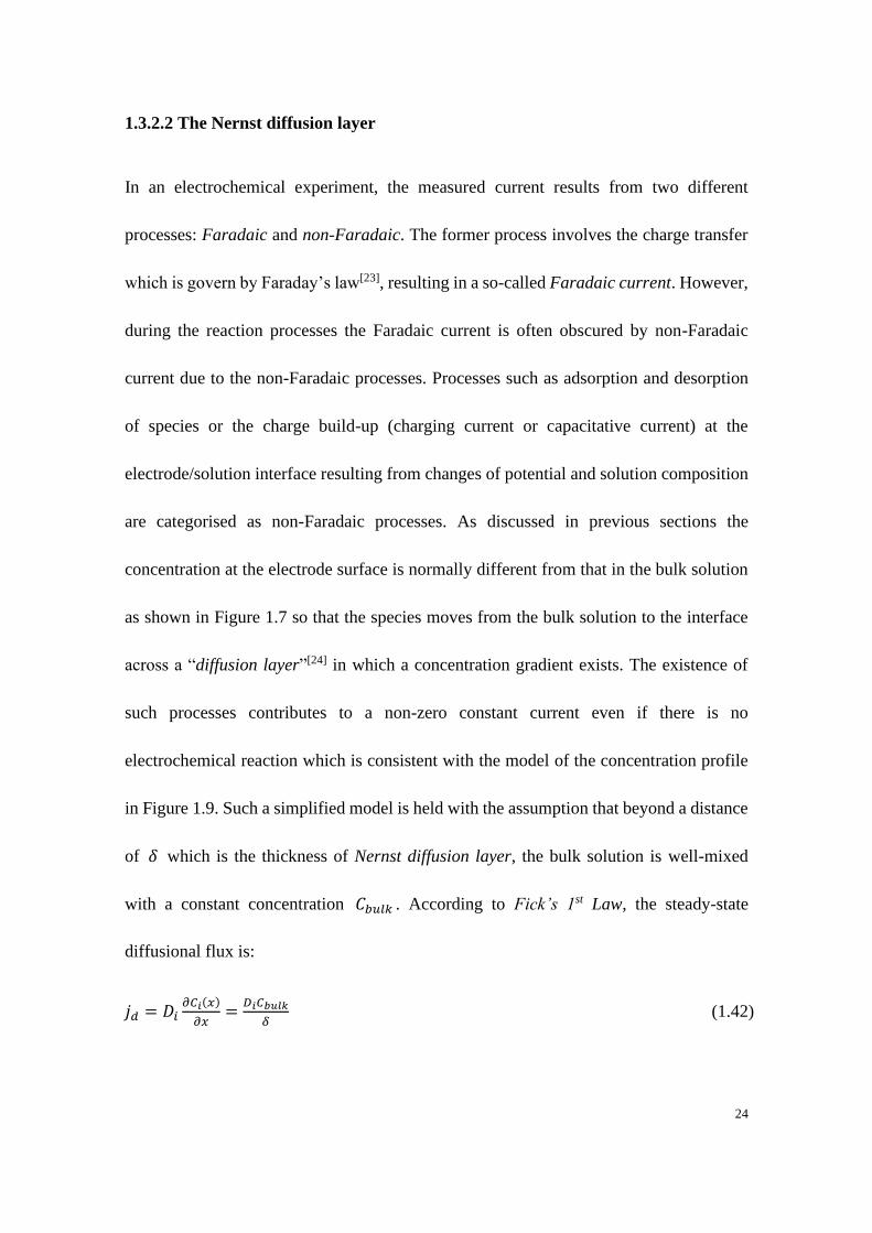
1.3.2.2 The Nernst diffusion layer
In an electrochemical experiment, the measured current results from two different
processes: Faradaic and non-Faradaic. The former process involves the charge transfer
which is govern by Faraday’s law[23], resulting in a so-called Faradaic current. However,
during the reaction processes the Faradaic current is often obscured by non-Faradaic
current due to the non-Faradaic processes. Processes such as adsorption and desorption
of species or the charge build-up (charging current or capacitative current) at the
electrode/solution interface resulting from changes of potential and solution composition
are categorised as non-Faradaic processes. As discussed in previous sections the
concentration at the electrode surface is normally different from that in the bulk solution
as shown in Figure 1.7 so that the species moves from the bulk solution to the interface
across a “diffusion layer”[24] in which a concentration gradient exists. The existence of
such processes contributes to a non-zero constant current even if there is no
electrochemical reaction which is consistent with the model of the concentration profile
in Figure 1.9. Such a simplified model is held with the assumption that beyond a distance
of 𝛿 which is the thickness of Nernst diffusion layer, the bulk solution is well-mixed
with a constant concentration 𝐶𝑏𝑢𝑙𝑘 . According to Fick’s 1st Law, the steady-state
diffusional flux is:
𝑗𝑑 = 𝐷𝑖𝜕𝐶𝑖(𝑥)
𝜕𝑥=
𝐷𝑖𝐶𝑏𝑢𝑙𝑘
𝛿 (1.42)
25
The corresponding steady-state current 𝐼𝑠.𝑠 at the electrode with a Nernst diffusion layer
of thickness is:
𝐼𝑠.𝑠 = 𝑛𝐹𝐴𝑗𝑑 =𝑛𝐹𝐴𝐷𝑖𝐶𝑏𝑢𝑙𝑘
𝛿 (1.43)
Here a so-called mass transport diffusion coefficient is defined as:[6]
𝑚0 =𝐷𝑖
𝛿 (1.44)
where the unit of 𝑚0 is cm s-1 which is the same as that of the electrochemical rate
constant, allowing the direct comparison between the mass transfer of species and the
electrode kinetics as will be discussed in section 1.4.
Figure 1.9 Nernst diffusion layer[24]. The y-axis is the concentration and x-axis is the distance from the
electrode surface.

26
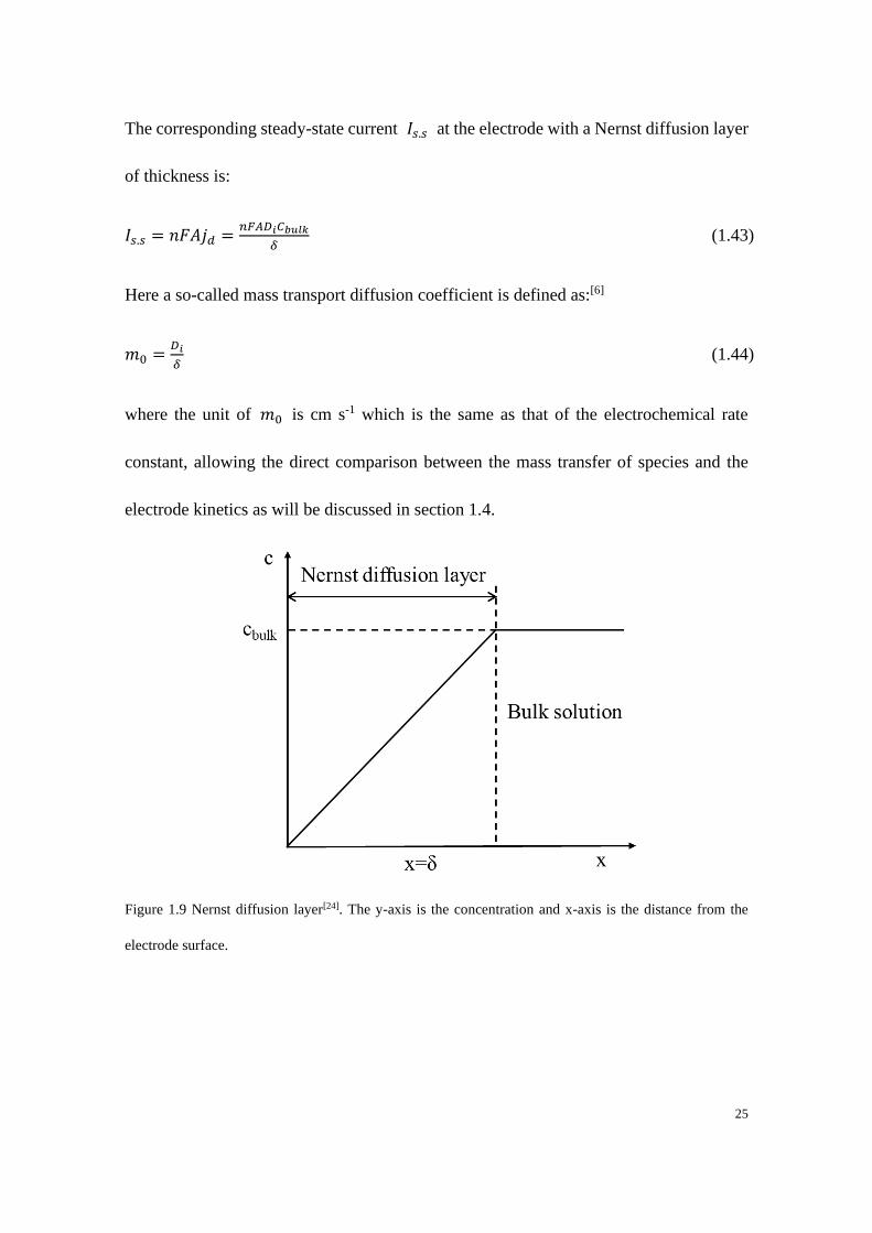
1.4 Electrochemical techniques: cyclic voltammetry
As is discussed above, the three-electrode cell in an electrochemical system is controlled
by a potentiostat through which the current or the potential can be applied to the working
electrode. Cyclic voltammetry (CV) is a simple but powerful method which is widely
employed in the study of electrode kinetics in electrochemical systems.[25] In cyclic
voltammetry the potential is applied at the working electrode as a function of time,
resulting in a corresponding voltammetric current response as a function of applied
potential.[26] CV is similar to linear sweep voltammetry but the potential in this case is
reversed back to the starting potential. Here we consider a simple one electron transfer
reductive process 𝐴 + 𝑒− ⇌ 𝐵 where A and B are in aqueous solution and initially only
A exists. The potential is applied to the working electrode in a way illustrated in Figure
1.10 where the starting potential is labelled as E1 at which point usually no
electrochemical reaction happens so that the electroactive species of interest at first
remains in its initial state. The potential is then swept linearly to E2 with a fixed scan rate
ν, at which point the direction of scan is reversed and swept back to E1. The potential
window (E1-E2) is chosen so that the electrochemical reaction under investigation occurs
over such potential range. The resulting voltammetric current response as a function of
the applied potential is known as a cyclic voltammogram.
27
Figure 1.10 The potential-time profile for a cyclic voltammetry.
1.4.1 Reversibility: mass transport versus electrode kinetics
Here we still consider a one-electron transfer process (reaction 1.16) in aqueous solution.
(1.16)
When a potential is applied to the working electrode at which point the potential is
negative enough to reduce A to B or positive enough to oxidise B to A, there is a
competition between how fast the species is transferred to the interface (mass transport)
and the species is reduced or oxidised (electrode kinetics). The rate of mass transport is
measured by the mass transport coefficient 𝑚0 =𝐷𝑖
𝛿,[6] where 𝛿 is dependent on time t
(𝛿~√𝐷𝑡).
According to 𝐸~𝑅𝑇
𝐹, then the time 𝑡~
𝑅𝑇
𝐹𝜈 where ν is the scan rate in V s-1, consequently,
the mass transport coefficient for a cyclic voltammetric experiment can be estimated by:
𝑚0 = √𝐷
(𝑅𝑇𝐹𝜈⁄ )
(1.45)
28
The rate of electrode kinetics is measured using the standard electrochemical rate constant
k0, therefore the process is considered as reversible if 𝑘0 ≫ 𝑚0 and irreversible if
𝑘0 ≪ 𝑚0. The transition between the reversible and irreversible limit is considered as
quasi-reversible or quasi-irreversible process. How the voltammetric behaviour varies
with reversibility is discussed in the following sections.
1.4.2 Cyclic voltammetry at different electrode geometries
Working electrodes normally used in electrochemical measurements are categorised as
either macroelectrodes or microelectrodes in terms of the size of the electrodes.
Macroelectrodes are large electrodes with dimensions usually in the millimetre scale. A
microelectrode has a definition by the International Union of Pure and Applied Chemistry
(IUPAC) that a microelectrode has at least one dimension of tens of micrometers or less,
down to the submicrometer range.[14] For electrodes with dimensions in less than
micrometre scale, other terms, for example, ultramicroelectrodes[27] and
nanoelectrodes[28], are sometimes used in the literature. The size difference among
electrodes results in distinguishable diffusional profiles and hence different voltammetric
behaviours. In the following, discussion is divided into three regimes in terms of their
diffusion profile and mass-transport regime: linear diffusion, steady-state and quasi-
steady state. Note that the reaction considered is reaction (1.16) throughout this chapter
unless otherwise stated.
29
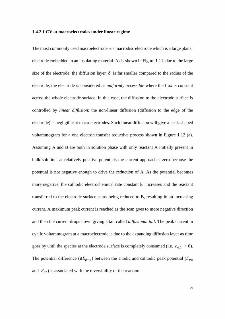
1.4.2.1 CV at macroelectrodes under linear regime
The most commonly used macroelectrode is a macrodisc electrode which is a large planar
electrode embedded in an insulating material. As is shown in Figure 1.11, due to the large
size of the electrode, the diffusion layer 𝛿 is far smaller compared to the radius of the
electrode, the electrode is considered as uniformly accessible where the flux is constant
across the whole electrode surface. In this case, the diffusion to the electrode surface is
controlled by linear diffusion; the non-linear diffusion (diffusion to the edge of the
electrode) is negligible at macroelectrodes. Such linear diffusion will give a peak-shaped
voltammogram for a one electron transfer reductive process shown in Figure 1.12 (a).
Assuming A and B are both in solution phase with only reactant A initially present in
bulk solution, at relatively positive potentials the current approaches zero because the
potential is not negative enough to drive the reduction of A. As the potential becomes
more negative, the cathodic electrochemical rate constant kc increases and the reactant
transferred to the electrode surface starts being reduced to B, resulting in an increasing
current. A maximum peak current is reached as the scan goes to more negative direction
and then the current drops down giving a tail called diffusional tail. The peak current in
cyclic voltammogram at a macroelectrode is due to the expanding diffusion layer as time
goes by until the species at the electrode surface is completely consumed (i.e. 𝑐𝐴,0 → 0).
The potential difference (Δ𝐸𝑝−𝑝) between the anodic and cathodic peak potential (𝐸𝑝𝑎
and 𝐸𝑝𝑐) is associated with the reversibility of the reaction.

30
Figure 1.11 Diffusion profile at a macrodisc electrode.
Figure 1.12(b) shows the voltammograms on a macroelectrode with different
electrochemical rate constants (red – reversible; blue – quasi-reversible; yellow –
irreversible). As k0 decreases, the peak-to-peak separation (Δ𝐸𝑝−𝑝) becomes larger which
indicates the process is becoming more irreversible. For the fully irreversible process,
ideally there is a potential region where the net current is zero, implying that a significant
potential above the thermodynamically required potential need to be applied to drive the
process of the reaction. However, in the reversible limit with fast electrode kinetics
(relative to the mass transport), apparent current flow is observed at the potential near
equilibrium potential at which point the Nernst equilibrium is attained. The concentration
at the electrode surface for a fully reversible process then follows Nernst equation:
𝐸 = 𝐸𝑓,𝐴/𝐵⦵ −
𝑅𝑇
𝐹𝑙𝑛
𝑐𝐵,0
𝑐𝐴,0 (1.46)
where 𝑐𝐴,0 and 𝑐𝐵,0 are the concentrations of species A and B at the electrode surface.
Another important parameter obtained from the voltammogram is the mid-point potential:
𝐸𝑚𝑖𝑑 =|𝐸𝑝𝑎−𝐸𝑝𝑐|
2 (1.47)

31
For a reversible process, 𝐸𝑚𝑖𝑑 is expressed as:
𝐸𝑚𝑖𝑑 = 𝐸𝑓,𝐴/𝐵⦵ −
𝑅𝑇
2𝐹𝑙𝑛
𝐷𝐵
𝐷𝐴 (1.48)
For an irreversible process with the anodic and cathodic transfer coefficients of 0.5, 𝐸𝑚𝑖𝑑
is expressed as:
𝐸𝑚𝑖𝑑 = 𝐸𝑓,𝐴/𝐵⦵ −
𝑅𝑇
𝐹𝑙𝑛
𝐷𝐵
𝐷𝐴 (1.49)
According to Equations (1.48) and (1.49), the formal potential of a redox couple A/B can
be estimated from its mid-point potential with the known knowledge of the ratio of the
diffusion coefficients of species A and B.
Figure 1.12 (a) Example of the cyclic voltammogram at a planar macrodisc electrode. (b) Voltammogram
on a macrodisc electrode with different electrochemical rate constants k0.
32
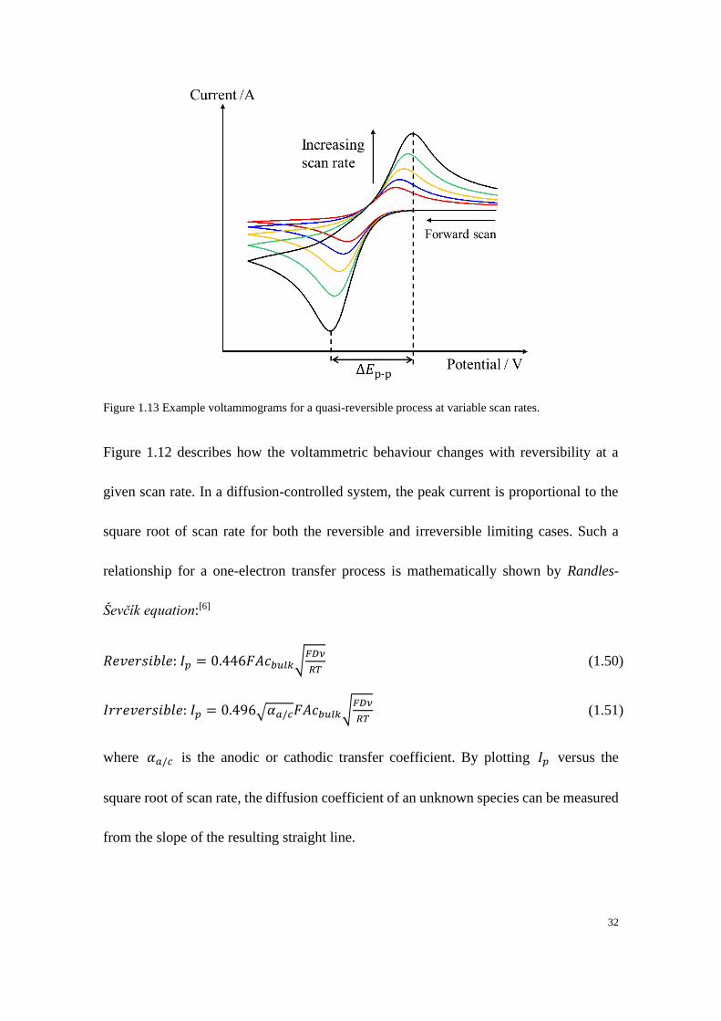
Figure 1.13 Example voltammograms for a quasi-reversible process at variable scan rates.
Figure 1.12 describes how the voltammetric behaviour changes with reversibility at a
given scan rate. In a diffusion-controlled system, the peak current is proportional to the
square root of scan rate for both the reversible and irreversible limiting cases. Such a
relationship for a one-electron transfer process is mathematically shown by Randles-
Ševčík equation:[6]
𝑅𝑒𝑣𝑒𝑟𝑠𝑖𝑏𝑙𝑒: 𝐼𝑝 = 0.446𝐹𝐴𝑐𝑏𝑢𝑙𝑘√𝐹𝐷𝜈
𝑅𝑇 (1.50)
𝐼𝑟𝑟𝑒𝑣𝑒𝑟𝑠𝑖𝑏𝑙𝑒: 𝐼𝑝 = 0.496√𝛼𝑎/𝑐𝐹𝐴𝑐𝑏𝑢𝑙𝑘√𝐹𝐷𝜈
𝑅𝑇 (1.51)
where 𝛼𝑎/𝑐 is the anodic or cathodic transfer coefficient. By plotting 𝐼𝑝 versus the
square root of scan rate, the diffusion coefficient of an unknown species can be measured
from the slope of the resulting straight line.
33
Figure 1.13 shows an example of how the voltammogram changes at different scan rates
for a quasi-reversible process. There are two changes to the voltammetric response as the
scan rate increases: 1) the magnitude of current increases at higher scan rates; 2) the peak-
to-peak separation increases at higher scan rates, indicating an increased irreversibility.
Since the thickness of diffusion layer built up during the voltammogram increases with
the time taken of the scan, for the same potential window, a higher scan rate requires
shorter time to build up the diffusion layer around the electrode, resulting in a thinner
diffusion layer which gives a large concentration gradient. According to Fick’s 1st Law,
a larger concentration gradient produces a higher current flux. In addition since the
thickness of diffusion layer influences the rate of mass transfer as discussed in section
1.4.1, the ratio between the mass transport and the electrode kinetics becomes relatively
large, which encourages electrochemical irreversibility at higher scan rates.
For processes involving more than one electron transfer, the current can be predicted by:
𝑅𝑒𝑣𝑒𝑟𝑠𝑖𝑏𝑙𝑒: 𝐼𝑝 = 0.446𝑛𝐹𝐴𝑐𝑏𝑢𝑙𝑘√𝑛𝐹𝐷𝜈
𝑅𝑇 (1.52)
𝐼𝑟𝑟𝑒𝑣𝑒𝑟𝑠𝑖𝑏𝑙𝑒: 𝐼𝑝 = 0.496√𝑛′ + 𝛼𝑛′+1𝑛𝐹𝐴𝑐𝑏𝑢𝑙𝑘√𝐹𝐷𝜈
𝑅𝑇 (1.53)
where 𝑛 is the number of electrons transferred, 𝑛′ is the total number of electrons
transferred before the rate determining step and 𝛼𝑛′+1 is the transfer coefficient of the
rate determining step.
34
1.4.2.2 CV at microelectrodes under a steady-state diffusion regime
Two types of electrode geometries are discussed in this section: the microdisc electrode
and the micro-hemispherical electrode (a spherical electrode is similar but with the only
difference of double the current magnitude). The diffusional profiles at the
microelectrodes with both geometries are shown in Figure 1.14 where the electrode radius
is much smaller than the steady-state diffusion layer thickness (𝑟 ≪ √𝐷𝜋𝑡). Unlike the
peak-shaped voltammogram at macroelectrodes, a steady-state flux can be achieved
without stirring of the solution as a consequence of radial diffusion. Such radial diffusion
improves the efficiency of mass transport, resulting in a sigmoidal voltammogram with a
steady-state current 𝐼𝑠.𝑠 at sufficiently slow scan rates. When the potential is applied to
the electrode, at very short time limit, the diffusion layer built-up is still much smaller
compared to the radius of electrode (𝑟 ≫ √𝐷𝜋𝑡), which corresponds to the response
obtained under linear diffusion as discussed in the previous sections. As time goes by, the
diffusion layer becomes thicker and thicker until 𝑟 ≪ √𝐷𝜋𝑡 at long-time limit.
Here the current on a uniformly accessible (hemi)spherical electrode is given as:
𝐼𝑠.𝑠 = 2𝜋𝑟𝐷𝐹𝑐𝑏𝑢𝑙𝑘 (ℎ𝑒𝑚𝑖𝑠𝑝ℎ𝑒𝑟𝑖𝑐𝑎𝑙 𝑒𝑙𝑒𝑐𝑡𝑟𝑜𝑑𝑒) (1.54)
𝐼𝑠.𝑠 = 4𝜋𝑟𝐷𝐹𝑐𝑏𝑢𝑙𝑘 (𝑠𝑝ℎ𝑒𝑟𝑖𝑐𝑎𝑙 𝑒𝑙𝑒𝑐𝑡𝑟𝑜𝑑𝑒) (1.55)
For the microdisc electrode of which the transient behaviour reflects a 2D diffusional
problem. Under steady-state conditions, the current to the electrode is given by Equation
(1.56) as originally described by Saito.[29]

35
𝐼𝑠.𝑠 = 4𝑛𝐹𝐷𝑐𝑏𝑢𝑙𝑘𝑟 (1.56)
From Equations (1.54), (1.55) and (1.56), the steady-state current on a microelectrode is
independent of scan rate, which provides an easier way for the measurement of the
diffusion coefficient of a species.
Figure 1.14 Diffusion profile for a (a) microdisc electrode and (b) micro hemispherical electrode.
Similar to the cases on macroelectrodes, the voltammetric behaviour is influenced by the
reversibility of the processes. Figure 1.15 shows examples of the voltammograms at a
micro-hemispherical electrode with variable electrochemical rate constants. In this case,
the half-wave potential (𝐸1/2) at which point the current is half of the steady-state current
is given by:
𝑅𝑒𝑣𝑒𝑟𝑠𝑖𝑏𝑙𝑒: 𝐸1/2 = 𝐸𝑓,𝐴/𝐵⦵ +
𝑅𝑇
𝑛𝐹ln (
𝐷𝐵
𝐷𝐴) (1.57)
𝐼𝑟𝑟𝑒𝑣𝑒𝑟𝑠𝑖𝑏𝑙𝑒: 𝐸1/2 = 𝐸𝑓,𝐴/𝐵⦵ +
𝑅𝑇
𝛼𝐹ln (
𝑟𝑘0
𝐷𝐴) (1.58)
From the above two equations, the formal potential can be estimated for a reversible
process with the knowledge of the ratio of diffusion coefficients of reactant and product;
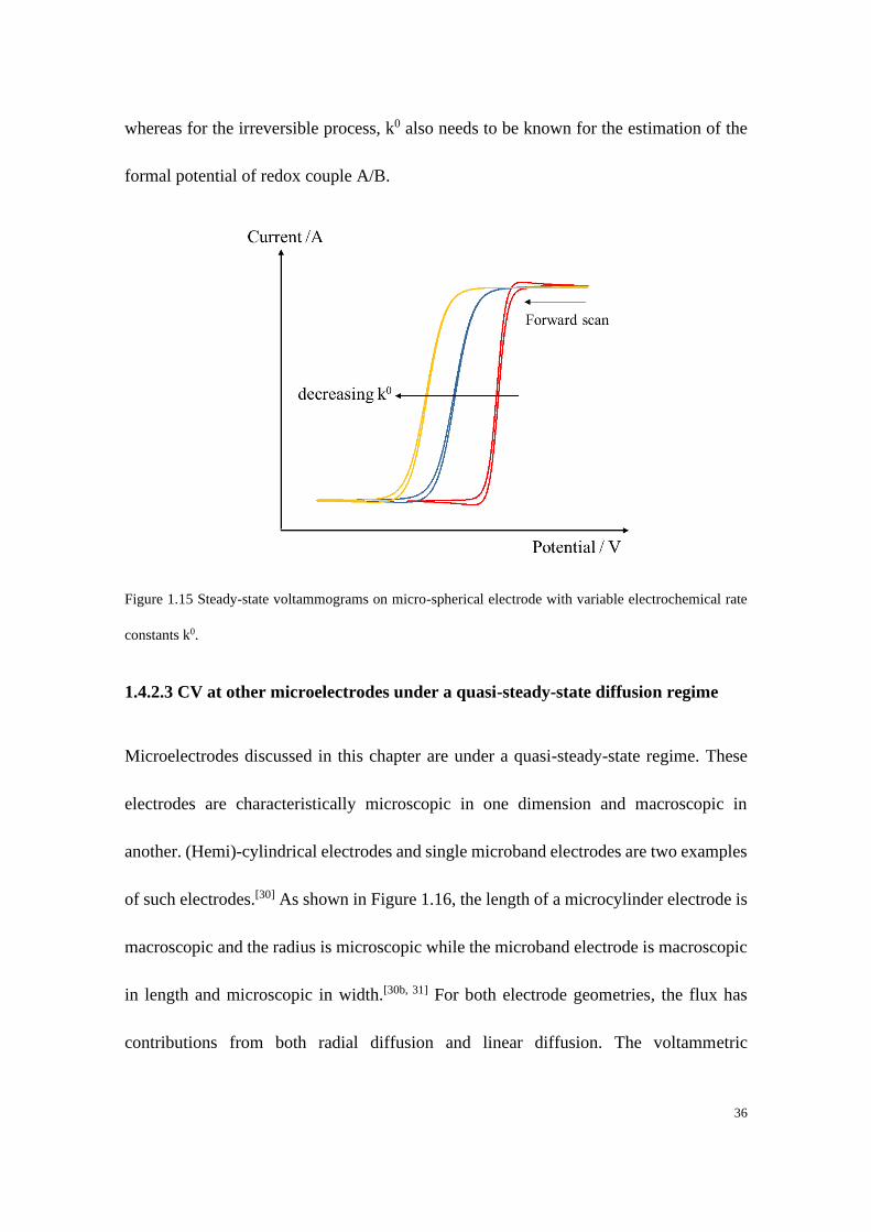
36
whereas for the irreversible process, k0 also needs to be known for the estimation of the
formal potential of redox couple A/B.
Figure 1.15 Steady-state voltammograms on micro-spherical electrode with variable electrochemical rate
constants k0.
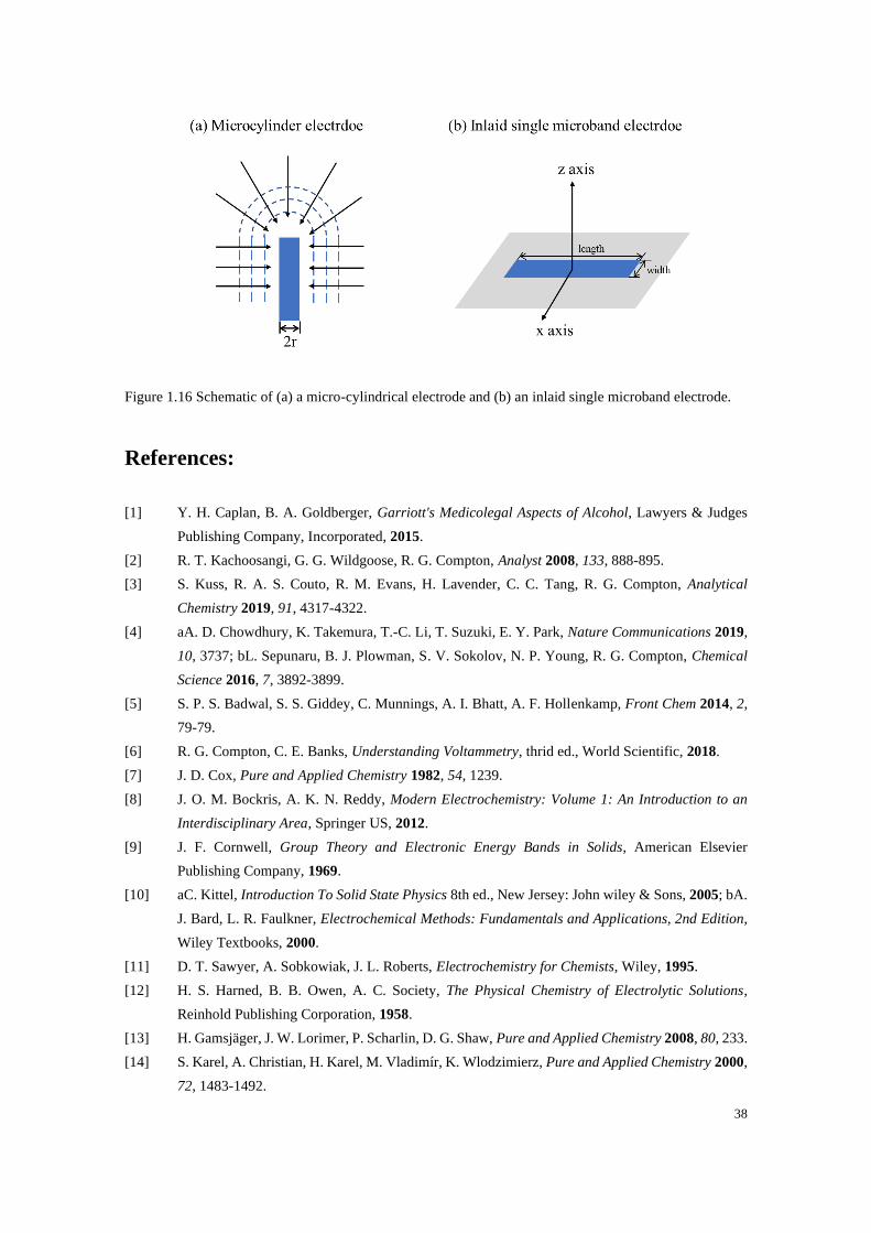
1.4.2.3 CV at other microelectrodes under a quasi-steady-state diffusion regime
Microelectrodes discussed in this chapter are under a quasi-steady-state regime. These
electrodes are characteristically microscopic in one dimension and macroscopic in
another. (Hemi)-cylindrical electrodes and single microband electrodes are two examples
of such electrodes.[30] As shown in Figure 1.16, the length of a microcylinder electrode is
macroscopic and the radius is microscopic while the microband electrode is macroscopic
in length and microscopic in width.[30b, 31] For both electrode geometries, the flux has
contributions from both radial diffusion and linear diffusion. The voltammetric
37
waveshape on such electrodes is intermediate between peak-shaped and sigmoidal
voltammogram and the voltammetric response has a scan rate dependency.
In the long-time limit, the current at a micro-cylindrical electrode can be predicted
from:[10b]
𝐼𝑞𝑠𝑠 =2𝑛𝐹𝐴𝐷𝑐𝑏𝑢𝑙𝑘
𝑟𝑙𝑛𝜏 (1.59)
where 𝐼𝑞𝑠𝑠 is the quasi-steady-state current and 𝜏 =4𝐷𝑡
𝑟2 . The measured current is
proportional to the inverse logarithm of time, resulting in a rather slow decay of current
in the long-time limit compared to that for the macroelectrodes.
For the single microband electrode which is a two-dimensional problem, the current at a
microband electrode is often approximated to that of a hemi-cylinder of equivalent area
(𝑟 = 𝑤/𝜋).[19, 30a, 32] At long-time limit, the current at a single microband electrode can
be expressed as:[10b]
𝐼𝑞𝑠𝑠 =2𝜋𝑛𝐹𝐴𝐷𝑐𝑏𝑢𝑙𝑘
𝑤𝑙𝑛(64𝐷𝑡
𝑤2 ) (1.60)
Therefore, neither of the two electrode geometries is able to reach a true steady-state
current at long times.
38
Figure 1.16 Schematic of (a) a micro-cylindrical electrode and (b) an inlaid single microband electrode.
References:
[1] Y. H. Caplan, B. A. Goldberger, Garriott's Medicolegal Aspects of Alcohol, Lawyers & Judges
Publishing Company, Incorporated, 2015.
[2] R. T. Kachoosangi, G. G. Wildgoose, R. G. Compton, Analyst 2008, 133, 888-895.
[3] S. Kuss, R. A. S. Couto, R. M. Evans, H. Lavender, C. C. Tang, R. G. Compton, Analytical
Chemistry 2019, 91, 4317-4322.
[4] aA. D. Chowdhury, K. Takemura, T.-C. Li, T. Suzuki, E. Y. Park, Nature Communications 2019,
10, 3737; bL. Sepunaru, B. J. Plowman, S. V. Sokolov, N. P. Young, R. G. Compton, Chemical
Science 2016, 7, 3892-3899.
[5] S. P. S. Badwal, S. S. Giddey, C. Munnings, A. I. Bhatt, A. F. Hollenkamp, Front Chem 2014, 2,
79-79.
[6] R. G. Compton, C. E. Banks, Understanding Voltammetry, thrid ed., World Scientific, 2018.
[7] J. D. Cox, Pure and Applied Chemistry 1982, 54, 1239.
[8] J. O. M. Bockris, A. K. N. Reddy, Modern Electrochemistry: Volume 1: An Introduction to an
Interdisciplinary Area, Springer US, 2012.
[9] J. F. Cornwell, Group Theory and Electronic Energy Bands in Solids, American Elsevier
Publishing Company, 1969.
[10] aC. Kittel, Introduction To Solid State Physics 8th ed., New Jersey: John wiley & Sons, 2005; bA.
J. Bard, L. R. Faulkner, Electrochemical Methods: Fundamentals and Applications, 2nd Edition,
Wiley Textbooks, 2000.
[11] D. T. Sawyer, A. Sobkowiak, J. L. Roberts, Electrochemistry for Chemists, Wiley, 1995.
[12] H. S. Harned, B. B. Owen, A. C. Society, The Physical Chemistry of Electrolytic Solutions,
Reinhold Publishing Corporation, 1958.
[13] H. Gamsjäger, J. W. Lorimer, P. Scharlin, D. G. Shaw, Pure and Applied Chemistry 2008, 80, 233.
[14] S. Karel, A. Christian, H. Karel, M. Vladimír, K. Wlodzimierz, Pure and Applied Chemistry 2000,
72, 1483-1492.
39
[15] D. G. Truhlar, W. L. Hase, J. T. Hynes, The Journal of Physical Chemistry 1983, 87, 2664-2682.
[16] R. Guidelli, R. G. Compton, J. M. Feliu, E. Gileadi, J. Lipkowski, W. Schmickler, S. Trasatti, Pure
and Applied Chemistry 2014, 86, 259-262.
[17] T. Erdey-Grúz, M. Volmer, Zeitschrift für physikalische Chemie 1930, 150, 203-213.
[18] R. Guidelli, R. G. Compton, J. M. Feliu, E. Gileadi, J. Lipkowski, W. Schmickler, S. Trasatti, Pure
and Applied Chemistry 2014, 86, 245-258.
[19] R. G. A. B. Compton, Craig E, Understanding Voltammetry, third ed., World Scientific, 2018.
[20] J. Agar, Discussions of the Faraday Society 1947, 1, 26-37.
[21] aA. Fick, Annalen der Physik 1855, 170, 59; bA. Fick, The London, Edinburgh, and Dublin
Philosophical Magazine and Journal of Science 1855, 10, 30-39.
[22] J. Crank, The mathematics of diffusion Clarendon Press, Oxford [England], 1975.
[23] aM. Faraday, Philosophical Transactions of the Royal Society of London 1834, 124, 55-76; bM.
Faraday, Philosophical Transactions of the Royal Society of London 1834, 124, 77-122.
[24] N. Ibl, Pure and Applied Chemistry 1981, 53, 1827.
[25] N. Elgrishi, K. J. Rountree, B. D. McCarthy, E. S. Rountree, T. T. Eisenhart, J. L. Dempsey,
Journal of Chemical Education 2018, 95, 197-206.
[26] D. Pletcher, S. E. Group, R. Greff, R. Peat, L. M. Peter, J. Robinson, Instrumental Methods in
Electrochemistry, Elsevier Science, 2001.
[27] aElectroanalysis 2002, 14, 1041-1051; bJ. Heinze, Angewandte Chemie International Edition in
English 1993, 32, 1268-1288.
[28] Analyst 2004, 129, 1157-1165.
[29] Y. Saito, Review of Polarography 1968, 15, 177-187.
[30] aC. A. Amatore, B. Fosset, M. R. Deakin, R. M. Wightman, Journal of Electroanalytical
Chemistry and Interfacial Electrochemistry 1987, 225, 33-48; bM. P. Nagale, I. Fritsch, Analytical
Chemistry 1998, 70, 2908-2913.
[31] M. P. Nagale, I. Fritsch, Analytical Chemistry 1998, 70, 2902-2907.
[32] A. Szabo, D. K. Cope, D. E. Tallman, P. M. Kovach, R. M. Wightman, Journal of
Electroanalytical Chemistry and Interfacial Electrochemistry 1987, 217, 417-423.

40
Chapter 2
Experimental
This chapter presents first the generic details of experiments reported in this thesis
including the chemical reagents, the instrumentation and the preparation and geometries
of the electrodes. Second, the simulation programmes used in the thesis are outlined.
More details regarding bespoke experiments, are separately described in the relevant
Chapters 3-8.
2.1 Chemical reagents
All the chemical reagents used are listed in Table 2.1. Concentrations of each solution
used in individual experiments are described in relevant chapters 3-8. All the solutions
were prepared using deionised water (Milipore) with a resistivity of 18.2 MΩ cm at 25
oC.
Table 2.1 Chemical reagents used in the thesis.
Chemical Name Formula Purity Supplier
Ammonium iron (II) sulfate
hexahydrate
(NH4)2Fe(SO4)2 99.0% Aldrich
Ammonium iron (III) sulfate
dodecahydrate
NH4Fe(SO4)2 99.0% Aldrich
Ammonium sulfate (NH4)2SO4 ≥ 99.0% Aldrich
41
Ferrocenemethanol C11H12FeO
(FcCH2OH)
≥ 97% ChemCruz
Perchloric acid HClO4 70% Aldrich
Potassium chloride KCl ≥ 99.0% Sigma-Aldrich
Hexaammineruthenium (III)
chloride
[Ru(NH3)6]Cl3 ≥ 98.3% Alfa Aesar
Nitrogen gas N2 ≥ 99.99% BOC
2.2 Electrochemical instrumentation
All the experiments were performed with μAutolab Type III potentiostat using a standard
three-electrode setup in a grounded Faraday cage. The electrochemical cell was
thermostated at 25.0 (±0.1) oC unless otherwise stated through the use of either a
conventional water bath or a home-made optimised thermostated system (Figure 2.1).
This design of an optimised thermostated electrochemical cell was developed in previous
work in the Compton Group where a Peltier-effect heat pump (type ETH-127-14-15-RS,
R. S. Components Ltd, Corby, U.K.) was used to fabricate the thermostat system.[1] This
pump was 40 mm × 40 mm in area and 3.9 mm thick with a maximum cooling capacity
of 58.6 W and a maximum temperature difference of 65 K.[1] As shown in Figure 2.1, the
glass vial containing the solution and electrodes was held tightly in an aluminium block
with a cylindrical hole (23 mm in diameter; 40 mm in height) and the temperature control
of the solution was achieved by immersing a temperature probe into the solution.[1] The
Peltier element and the solution temperature were further monitored using a proportional-
integral-derivative (PID) loop script written in Python 3.5.[1] A saturated calomel
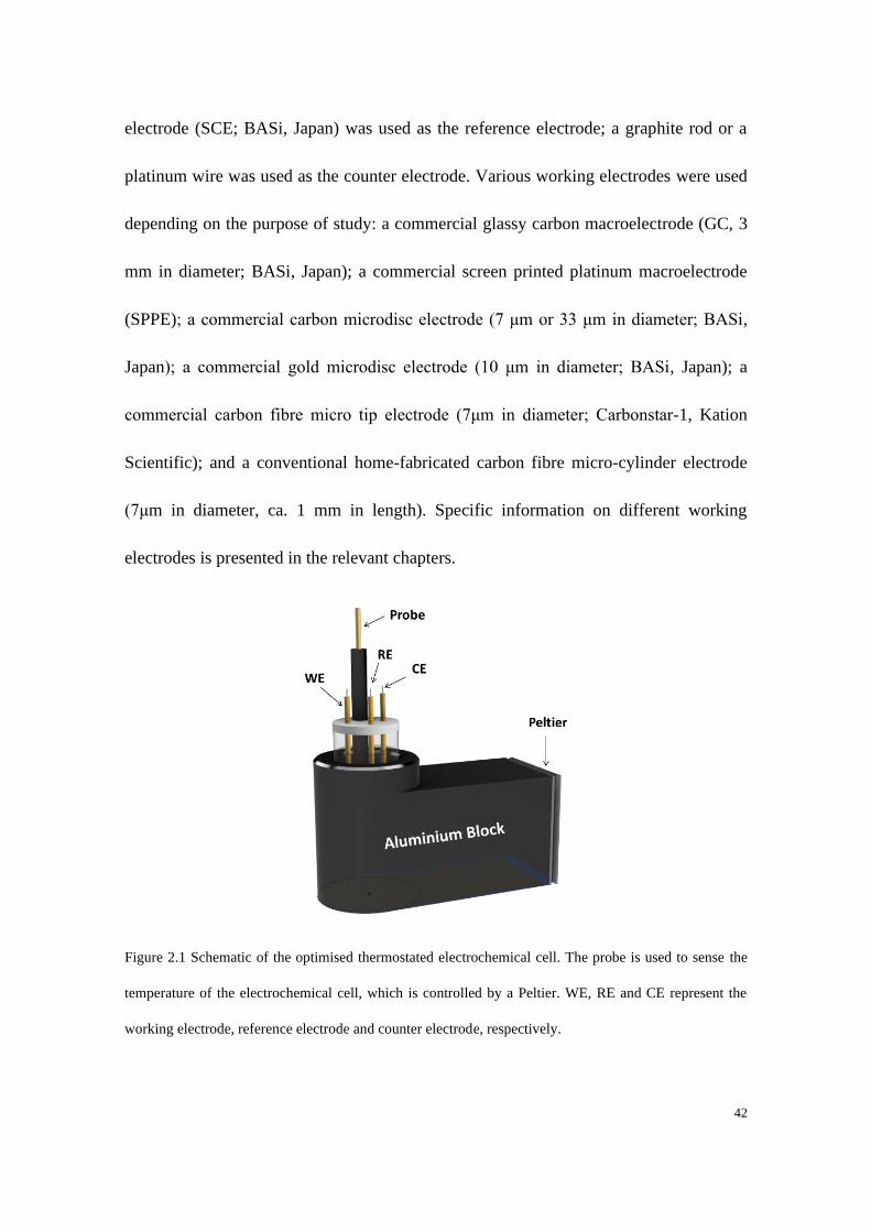
42
electrode (SCE; BASi, Japan) was used as the reference electrode; a graphite rod or a
platinum wire was used as the counter electrode. Various working electrodes were used
depending on the purpose of study: a commercial glassy carbon macroelectrode (GC, 3
mm in diameter; BASi, Japan); a commercial screen printed platinum macroelectrode
(SPPE); a commercial carbon microdisc electrode (7 μm or 33 μm in diameter; BASi,
Japan); a commercial gold microdisc electrode (10 μm in diameter; BASi, Japan); a
commercial carbon fibre micro tip electrode (7μm in diameter; Carbonstar-1, Kation
Scientific); and a conventional home-fabricated carbon fibre micro-cylinder electrode
(7μm in diameter, ca. 1 mm in length). Specific information on different working
electrodes is presented in the relevant chapters.
Figure 2.1 Schematic of the optimised thermostated electrochemical cell. The probe is used to sense the
temperature of the electrochemical cell, which is controlled by a Peltier. WE, RE and CE represent the
working electrode, reference electrode and counter electrode, respectively.
43
2.3 Preparation and geometries of the working electrodes
2.3.1 Preparation of the working electrodes
Macro- and microdisc electrode preparations All the commercial macro- or micro- disc
electrodes were, before use, polished using alumina of decreasing size (1.0, 0.3 and 0.05
μm, Buehler, IL) on a polishing pad, washed with deionised water and then dried with
nitrogen. The radii of macroelectrodes were determined using a travelling microscope
from at least three independent measurements. The radii of microdisc electrodes were
calibrated from the steady-state current obtained in a solution containing 1.0 mM
ferrocenemethanol and 0.1 M KCl using a diffusion coefficient for FcCH2OH of 7.81 ×
10-10 m2 s-1 at 25 oC or a solution containing 1.0 mM hexaammineruthenium chloride and
0.1 M KCl using a diffusion coefficient for [Ru(NH3)6]Cl3 of 8.43 × 10⁻¹⁰ m2 s-1 at 25
oC.[2]
Carbon fibre micro-cylinder electrode fabrication Carbon fibre micro-cylinder
electrodes were fabricated in-house using a method developed by Ellison et al.[3] A carbon
fibre (7 μm in diameter, Goodfellow, Cambridge, U.K.) was connected to a metal wire
using conductive silver epoxy adhesive (RS Components Ltd.) which was then cured in
the oven for 15 minutes at ca. 60 oC. The dried connection wire was then threaded through
a plastic pipette tip until only the carbon fire extended out of the pipette tip. A non-
conducting cyanoacrylate adhesive was used to seal the wire and the tip. The resulting
electrode was left overnight at room temperature to dry the glue. The desired wire
44
electrode was obtained by cutting the wire to approximately 1 mm length. The exact
length of the wire electrode was calibrated from the peak current of the voltammograms
obtained in a solution containing 1.0 mM ferrocenemethanol and 0.1 M KCl using a
diffusion coefficient for FcCH2OH of 7.81 × 10⁻¹⁰ m2 s-1 at 25 oC.[2] The electrode was
rinsed with deionised water before and after experiments. The geometry of the electrode
is shown in the following section.
2.3.2 Geometries of the working electrodes
The schematics of the electrode geometries used in this thesis are shown in Figure 2.2.
The commercial macro- and micro-disc electrodes are shown in Figure 2.2(a) and (b),
respectively. In both electrodes the electrode materials are embedded in an insulating
sheath. For the glassy carbon macrodisc electrode (Figure 2.2(a)), the calibrated diameter
was 2.984 (±0.005) mm and the total diameter of the electrode including the insulating
sheath was 6 mm. In Figure 2.2(b), the total diameter of microdisc electrode (i.e. including
the glass sheath) was 3.5 mm of which the diameter of the electrode material was only a
few micrometres. The carbon fibre used in the home-fabricated micro-cylinder electrode
(Figure 2.2(c)) was 7 μm in diameter of which the length was calibrated individually as
mentioned above. The carbon fibre micro tip electrode is shown in Figure 2.2(d) where
the diameter of the carbon fibre was 7 μm and the estimated length was ca. 15 μm.
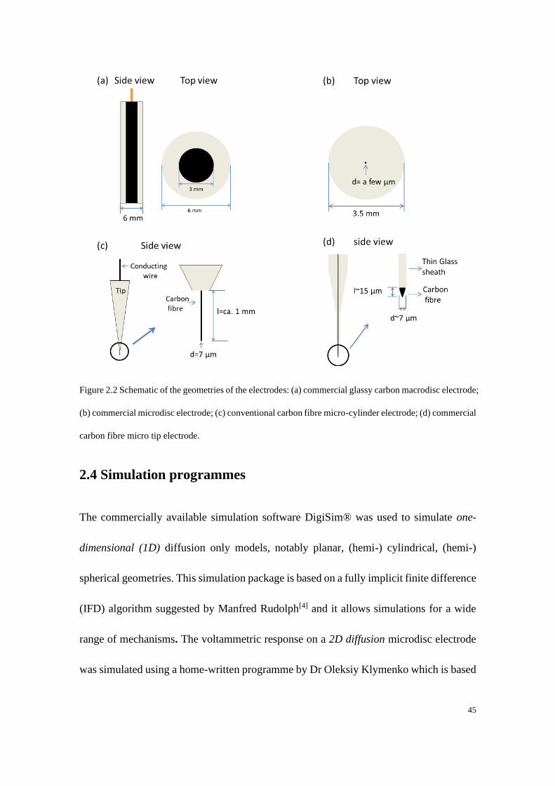
45
Figure 2.2 Schematic of the geometries of the electrodes: (a) commercial glassy carbon macrodisc electrode;
(b) commercial microdisc electrode; (c) conventional carbon fibre micro-cylinder electrode; (d) commercial
carbon fibre micro tip electrode.
2.4 Simulation programmes
The commercially available simulation software DigiSim® was used to simulate one-
dimensional (1D) diffusion only models, notably planar, (hemi-) cylindrical, (hemi-)
spherical geometries. This simulation package is based on a fully implicit finite difference
(IFD) algorithm suggested by Manfred Rudolph[4] and it allows simulations for a wide
range of mechanisms. The voltammetric response on a 2D diffusion microdisc electrode
was simulated using a home-written programme by Dr Oleksiy Klymenko which is based
46
on the conformal mapping of the spatial coordinates and uses an exponentially expanding
time grid.[5]
The voltammogram on a microband electrode was simulated using a bespoke programme
was written by Dr Chuhong Lin.[6] The numerical simulation procedures are introduced
further in detail in Chapters 4 and 6.
A home-written programme for a rotating disc electrode was written by Dr Christopher
Batchelor-McAuley. This simulation numerically calculates the voltammetric profile
using a fully implicit finite difference method and makes use of the Hale transform[7]
which is employed in Chapter 5.
References:
[1] X. Li, C. Batchelor-McAuley, J. K. Novev, R. G. Compton, Phys. Chem. Chem. Phys. 2018, 20,
11794-11804.
[2] K. Ngamchuea, C. Lin, C. Batchelor-McAuley, R. G. Compton, Analytical Chemistry 2017, 89,
3780-3786.
[3] J. Ellison, C. Batchelor-McAuley, K. Tschulik, R. G. Compton, Sensors and Actuators B:
Chemical 2014, 200, 47-52.
[4] aM. Rudolph, J. Electroanal. Chem. Interfacial Electrochem. 1991, 314, 13-22; bM. Rudolph, J.
Electroanal. Chem. 1992, 338, 85-98; cM. Rudolph, J. Electroanal. Chem. 1994, 375, 89-99.
[5] O. V. Klymenko, R. G. Evans, C. Hardacre, I. B. Svir, R. G. Compton, Journal of
Electroanalytical Chemistry 2004, 571, 211-221.
[6] D. Li, C. Lin, C. Batchelor-McAuley, L. Chen, R. G. Compton, Journal of Electroanalytical
Chemistry 2019, 840, 279-284.
[7] aR. G. Compton, E. Laborda, K. R. Ward, Understanding Voltammetry: Simulation Of Electrode
Processes, World Scientific Publishing Company, 2013; bJ. M. Hale, Journal of Electroanalytical
Chemistry (1959) 1963, 6, 187-197.
47
Chapter 3
Voltammetric Demonstration of Thermally Induced
Natural Convection in Aqueous Solution
Temperature control is normally used during electrochemical measurements since
changes in temperature affect the equilibrium potentials, diffusion coefficients, rate
constants (both homogeneous and heterogeneous), and hence the currents flowing. In
addition imperfect thermostating inevitably leads to the presence of bulk convective flows.
Whilst as recognised by Nernst[1] the damping of these bulk convective flows next to a
solid surface, or at an electrode, leads to diffusional mass transport predominating locally,
this chapter questions the exclusivity of diffusional transport and provides hitherto
unexplored physical insights into how thermally induced flows in bulk solution can, on
both macro- and microelectrodes, influence a voltammetric measurement. Imperfect
thermostating results in flows in the bulk solution which are predicted and here
experimentally shown to be as large as of the order of 100 μm s-1. We show that even in
the absence of natural convective flows induced by the electrochemical reaction itself,
this thermally induced bulk convection can significantly affect the voltammetric response.
First, we show that evaporative losses from an open electrochemical cell can be sufficient
to produce convective flows that can alter the electrochemical response. Second,
electrodes with various sizes and geometries have been investigated and experimental
48
results evidence that the sensitivity of an electrode to these flows in bulk solution is to a
large extent controlled by the size of the surrounding non-conductive supporting substrate
used to insulate parts of the electrode.
This work presented in this chapter has been published as a first author paper in Physical
Chemistry Chemical Physics[2] and was carried out in collaboration with Dr. Christopher
Batchelor-McAuley and Mr. Lifu Chen.
3.1 Introduction
Voltammetry lies at the very centre of the study of electrode reactions and, as well as
being key to understanding catalysis and analysis, it offers a plethora of fundamental
insights across a diversity of problems. Regardless of whether potential steps, sweeps[3]
or pulses[4] are used, the current-voltage behaviour is generally interpreted on the basis of
a signal in which the mass-transport is controlled exclusively by diffusion except when
forced convection is introduced either by flowing the solution or rotating or vibrating the
electrode. However, even in the absence of deliberately imposed convection, so-called
natural convection can arise. As clarified by Levich[5] one mechanism by which this may
arise originally from the heterogeneous reaction and relate to changes in solution density
in the proximity of the reaction surface. Levich[5] identified two cases that can induce a
density change, namely first, the intrinsic exo- or endothermicity of the electrode
reactions locally altering the solution temperature and second, the local changes in
chemical composition induced by the electrolysis causing altered local densities. Levich[5]
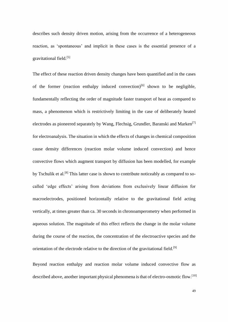
49
describes such density driven motion, arising from the occurrence of a heterogeneous
reaction, as ‘spontaneous’ and implicit in these cases is the essential presence of a
gravitational field.[5]
The effect of these reaction driven density changes have been quantified and in the cases
of the former (reaction enthalpy induced convection)[6] shown to be negligible,
fundamentally reflecting the order of magnitude faster transport of heat as compared to
mass, a phenomenon which is restrictively limiting in the case of deliberately heated
electrodes as pioneered separately by Wang, Flechsig, Grundler, Baranski and Marken[7]
for electroanalysis. The situation in which the effects of changes in chemical composition
cause density differences (reaction molar volume induced convection) and hence
convective flows which augment transport by diffusion has been modelled, for example
by Tschulik et al.[8] This latter case is shown to contribute noticeably as compared to so-
called ‘edge effects’ arising from deviations from exclusively linear diffusion for
macroelectrodes, positioned horizontally relative to the gravitational field acting
vertically, at times greater than ca. 30 seconds in chronoamperometry when performed in
aqueous solution. The magnitude of this effect reflects the change in the molar volume
during the course of the reaction, the concentration of the electroactive species and the
orientation of the electrode relative to the direction of the gravitational field.[9]
Beyond reaction enthalpy and reaction molar volume induced convective flow as
described above, another important physical phenomena is that of electro-osmotic flow.[10]
50
Such flows may be induced by applying an electric field in a perpendicular direction to a
double-layer. These flows have important technological applications in microfluidic
devices; however, they are of less direct relevance to electro-analytical systems and hence
will not be considered further in this work.
When theoretically analysing the influence of electrochemical reaction induced
convection (i.e. enthalpy or molar volume induced convection) it is common in
electrochemical simulations[8] to presume the presence of a stagnant bulk solution. Such
a situation requires a uniform temperature throughout the cell. This assumption has
recently been questioned and the simulation of typical electrochemical cells using finite
element methods has shown the existence of significant flows in bulk solution.[11] These
flows can arise from imperfect thermostating of a solution which is, at least to some extent,
intrinsic to the concept of maintaining a cell at a fixed temperature within surroundings
of different and variable temperatures. A common situation is that an electrochemical cell
is immersed in a thermostated water bath but also exposed to the air which may produce
a different temperature and/or allow evaporation from the water bath itself. Moreover if
the thermal conductivity of the wall in contact with the electrolytic solution is spatially
heterogeneous then local differential thermal conduction can lead to local solution phase
flows near the glass/solution interface inside the electrochemical cell. Furthermore and in
particular, evaporation of solvent from the surface of the liquid contained in the cell
locally reduces the temperature and can cause significant flows. These flows are driven
by the local temperature differences causing changes in the solution density. The
51
consequence of these effects is that even in the absence of other extrinsic forces (such as
vibrations) the bulk solution contains natural convective flows; due to imperfect
thermostating an aqueous solution will tend not towards a quiescent state but a convective
stationary one with a non-zero flow velocity. The question arises as to the extent to which
these density induced convective flows can influence voltammetry?
3.2 Experimental
3.2.1 Chemical reagents
Ferrocenemethanol (FcCH2OH; ChemCruz; >97%), Hexaammineruthenium (III)
chloride ([Ru(NH3)6]Cl3; Alfa Aesar; >98.3%) and potassium chloride (KCl; Sigma-
Aldrich; ≥ 99.0%) were used as purchased without further purification. Solutions (1 mM
FcCH2OH in 0.1 M KCl) were prepared using deionised water (Millipore) with a
resistivity of 18.2 MΩ cm.
3.2.2 Instrumentation
Electrochemical measurements were performed with a μAutolab Type III potentiostat
using a standard three electrode setup in an optimised thermostated electrochemical cell
(Scheme 3.1). This design was developed in previous work[12] and has been described in
Chapter 2. A saturated calomel electrode (SCE; BASi, Japan) and a platinum wire were
used as the reference electrode and the counter electrode, respectively. Five different
52
electrodes were used as working electrodes depending on the purpose of study as
mentioned below.
Scheme 3.1 Schematic of the optimised thermostated electrochemical cell. The probe is used to sense the
temperature of the electrochemical cell, which is controlled by a Peltier. WE, RE and CE represent the
working electrode, reference electrode and counter electrode, respectively.
3.2.3 Electrochemical cell designs for the study of convective effect on electrodes
with different geometries
All experiments were conducted in a glass vial (Specimen tubes soda glass, 50 × 23 mm,
SAMCO) containing 12 mL of solution (1 mM FcCH2OH in 0.1 M KCl) except where
otherwise stated. The side view of the set-up of the vial is shown in Scheme 3.2, in this
system the electrodes were positioned horizontally facing downward and at a height equal
to half of the solution depth.

53
Four different electrodes were used as working electrodes: a conventional carbon fibre
microcylinder electrode (7 μm in diameter), a commercial carbon fibre micro tip electrode
(7μm in diameter; Carbonstar-1, Kation Scientific), a commercial carbon microdisc
electrode (33 μm in diameter; BASi) and a commercial glassy carbon macroelectrode (3
mm in diameter; BASi). Prior to experiments, the latter two electrodes were polished
using alumina of decreasing size (1.0, 0.3 and 0.05 μm, Buehler, IL), washed with
deionised water and dried with nitrogen.
Scheme 3.2 Schematic of the side-view of the set-up within the glass vial. The surface of working electrode
shown here is horizontal facing downward.
Geometries of the electrodes The schematics of the electrode geometries are shown in
Scheme 3.3. For the commercial macrodisc electrode (Scheme 3.3(a)), the calibrated
diameter of glassy carbon is 2.984 (±0.005) mm and the total diameter of the electrode
(i.e. including the insulating sheath) is 6 mm; for the commercial microdisc electrode
(Scheme 3.3(b)), the diameter of carbon fibre is 33 μm and the total diameter of the
electrode (i.e. including the glass sheath) is 3.5 mm; for the conventional carbon fibre
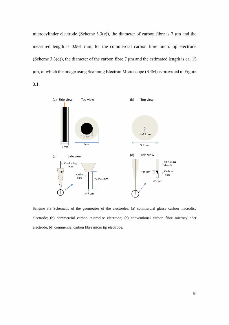
54
microcylinder electrode (Scheme 3.3(c)), the diameter of carbon fibre is 7 μm and the
measured length is 0.961 mm; for the commercial carbon fibre micro tip electrode
(Scheme 3.3(d)), the diameter of the carbon fibre 7 μm and the estimated length is ca. 15
μm, of which the image using Scanning Electron Microscope (SEM) is provided in Figure
3.1.
Scheme 3.3 Schematic of the geometries of the electrodes: (a) commercial glassy carbon macrodisc
electrode; (b) commercial carbon microdisc electrode; (c) conventional carbon fibre microcylinder
electrode; (d) commercial carbon fibre micro tip electrode.
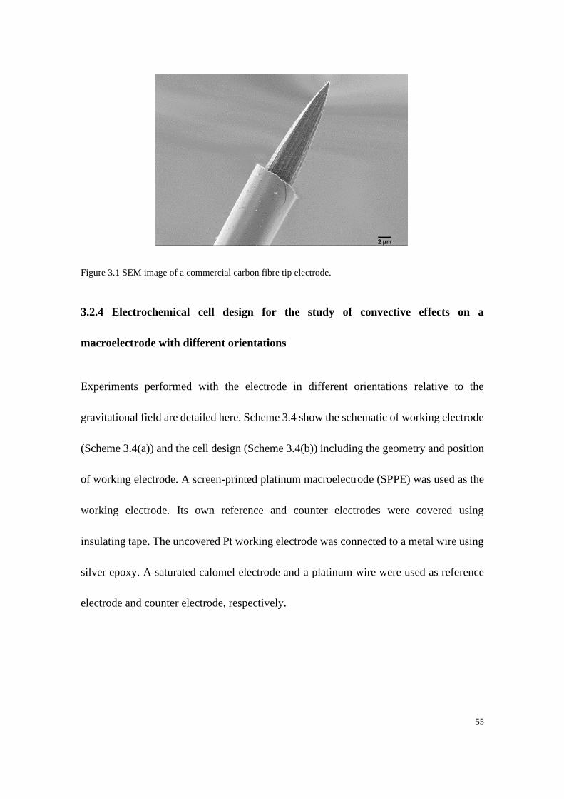
55
Figure 3.1 SEM image of a commercial carbon fibre tip electrode.
3.2.4 Electrochemical cell design for the study of convective effects on a
macroelectrode with different orientations
Experiments performed with the electrode in different orientations relative to the
gravitational field are detailed here. Scheme 3.4 show the schematic of working electrode
(Scheme 3.4(a)) and the cell design (Scheme 3.4(b)) including the geometry and position
of working electrode. A screen-printed platinum macroelectrode (SPPE) was used as the
working electrode. Its own reference and counter electrodes were covered using
insulating tape. The uncovered Pt working electrode was connected to a metal wire using
silver epoxy. A saturated calomel electrode and a platinum wire were used as reference
electrode and counter electrode, respectively.
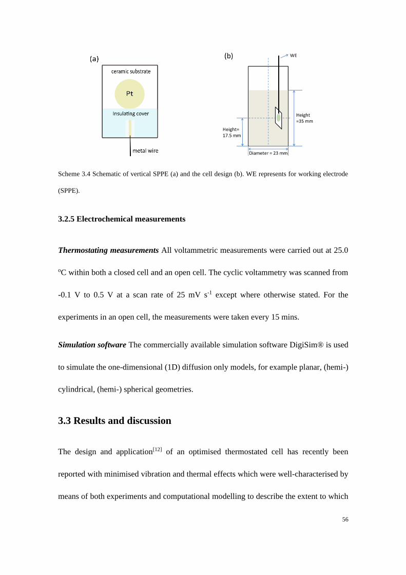
56
Scheme 3.4 Schematic of vertical SPPE (a) and the cell design (b). WE represents for working electrode
(SPPE).
3.2.5 Electrochemical measurements
Thermostating measurements All voltammetric measurements were carried out at 25.0
oC within both a closed cell and an open cell. The cyclic voltammetry was scanned from
-0.1 V to 0.5 V at a scan rate of 25 mV s-1 except where otherwise stated. For the
experiments in an open cell, the measurements were taken every 15 mins.
Simulation software The commercially available simulation software DigiSim® is used
to simulate the one-dimensional (1D) diffusion only models, for example planar, (hemi-)
cylindrical, (hemi-) spherical geometries.
3.3 Results and discussion
The design and application[12] of an optimised thermostated cell has recently been
reported with minimised vibration and thermal effects which were well-characterised by
means of both experiments and computational modelling to describe the extent to which
57
the full thermostating of a cell by a heated bath can be realised. The detailed design of
this optimised thermostated cell is described in above Section 3.2.2. The modelling
included heat transfer due to evaporation and radiative processes and, in agreement with
experiments, indicated that the steady-state temperature of the cell could deviate from
that of the thermostat by ~0.1 K. Such a spatial inhomogeneity of the temperature is
predicted to drive convective flows of speed of the order of 100 μm s-1 in bulk solution.[12]
3.3.1 Chronoamperometric responses on a macrodisc electrode
First, the oxidation of a model redox probe under relatively quiescent conditions is studied
in the electrochemical cell schematically shown in Scheme 3.1. Figure 3.2 shows the
chronoamperometric response of a glassy carbon macro-electrode (3 mm in diameter)
obtained by applying a constant positive potential of 0.35 V for 60 s for the oxidation of
1 mM ferrocenemethanol at 25 oC. In this experiment the working electrode is facing
downward, as would be most commonly done in an electroanalytical experiment.
Overlaid is the theoretical time current transient as predicted using a) the Cottrell
equation[3] and b) the Shoup-Szabo equation.[14] The Cottrell equation is given as
Equation 3.1:
𝐼 =𝑛𝐹𝐴√𝐷𝑐𝑏𝑢𝑙𝑘
√𝜋𝑡 (3.1)
The Shoup-Szabo equation is given as Equation 3.2 which additionally accounts for the
contribution of radial diffusion towards the macrodisc electrode.
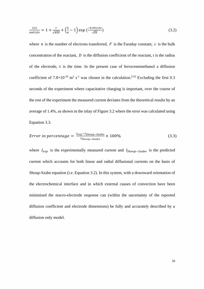
58
𝐼(𝑡)
𝑛𝜋𝐹𝑐𝐷𝑟= 1 +
𝑟
√𝜋𝐷𝑡+ (
4
𝜋− 1) exp (
−0.39115𝑟
√𝐷𝑡) (3.2)
where 𝑛 is the number of electrons transferred, 𝐹 is the Faraday constant, 𝑐 is the bulk
concentration of the reactant, 𝐷 is the diffusion coefficient of the reactant, r is the radius
of the electrode, 𝑡 is the time. In the present case of ferrocenemethanol a diffusion
coefficient of 7.8×10⁻¹⁰ m2 s-1 was chosen in the calculation.[15] Excluding the first 0.3
seconds of the experiment where capacitative charging is important, over the course of
the rest of the experiment the measured current deviates from the theoretical results by an
average of 1.4%, as shown in the inlay of Figure 3.2 where the error was calculated using
Equation 3.3.
𝐸𝑟𝑟𝑜𝑟 𝑖𝑛 𝑝𝑒𝑟𝑐𝑒𝑛𝑡𝑎𝑔𝑒 = 𝐼𝑒𝑥𝑝−𝐼𝑆ℎ𝑜𝑢𝑝−𝑆𝑧𝑎𝑏𝑜
𝐼𝑆ℎ𝑜𝑢𝑝−𝑆𝑧𝑎𝑏𝑜× 100% (3.3)
where 𝐼𝑒𝑥𝑝 is the experimentally measured current and 𝐼𝑆ℎ𝑜𝑢𝑝−𝑆𝑧𝑎𝑏𝑜 is the predicted
current which accounts for both linear and radial diffusional currents on the basis of
Shoup-Szabo equation (i.e. Equation 3.2). In this system, with a downward orientation of
the electrochemical interface and in which external causes of convection have been
minimised the macro-electrode response can (within the uncertainty of the reported
diffusion coefficient and electrode dimensions) be fully and accurately described by a
diffusion only model.

59
Figure 3.2 The experimentally recorded chronoamperometric response of a glassy carbon macrodisc
electrode (red) (r = 0.15 cm) plotted against that predicted on the basis of the Cottrell (blue) and Shoup-
Szabo equations (brown). Inlay in (a) depicts the error between the experimental (red) and simulated
chronoamperometric response that predicted by the Shoup-Szabo (brown). The excellent agreement of the
experimental data with the Shoup-Szabo equation highlights the importance of accounting for radial
diffusion at this time scale even when using an electrode of millimetres in dimension. The experiment was
run in a glass vial with 12 mL solution (1 mM FcCH2OH in 0.1 M KCl) at a constant applied potential of
+0.35 V with the macroelectrode facing downwards.
It should be noted that the Shoup-Szabo equation is itself approximate being based on
fitting to simulations and can be in error by up to 0.6%. Figure 3.3 below presents the plot
of the normalised difference ((𝐼𝑒𝑥𝑝 − 𝐼𝑠𝑖𝑚)/𝐼𝑠𝑖𝑚)) of choronoamperometric response for
the oxidation of 1 mM ferrocenemethanol at 25oC at a glassy carbon macroelectrode,
where 𝐼𝑒𝑥𝑝 is the experimental measured current and 𝐼𝑠𝑖𝑚 is the simulated current
response. The simulation was based on a two-dimensional microdisc model solved using
the ADI method.[16] This result shows that with the consideration of radial diffusion, the
0 10 20 30 40 50 60-6.0
-5.5
-5.0
-4.5
0 10 20 30 40 50 60-0.04
-0.02
0.00
0.02
0.04
0.06
Err
or
Time / s
log
10(c
urr
ent)
/ A
Time / s
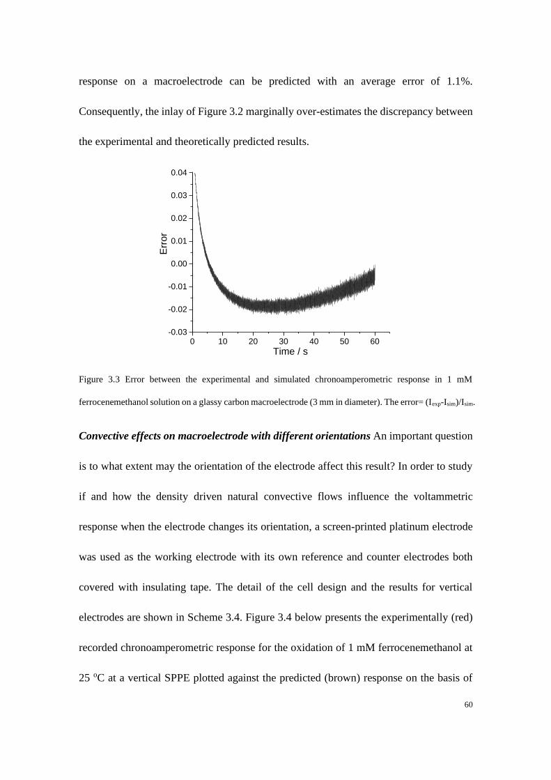
60
response on a macroelectrode can be predicted with an average error of 1.1%.
Consequently, the inlay of Figure 3.2 marginally over-estimates the discrepancy between
the experimental and theoretically predicted results.
Figure 3.3 Error between the experimental and simulated chronoamperometric response in 1 mM
ferrocenemethanol solution on a glassy carbon macroelectrode (3 mm in diameter). The error= (Iexp-Isim)/Isim.
Convective effects on macroelectrode with different orientations An important question
is to what extent may the orientation of the electrode affect this result? In order to study
if and how the density driven natural convective flows influence the voltammetric
response when the electrode changes its orientation, a screen-printed platinum electrode
was used as the working electrode with its own reference and counter electrodes both
covered with insulating tape. The detail of the cell design and the results for vertical
electrodes are shown in Scheme 3.4. Figure 3.4 below presents the experimentally (red)
recorded chronoamperometric response for the oxidation of 1 mM ferrocenemethanol at
25 oC at a vertical SPPE plotted against the predicted (brown) response on the basis of
0 10 20 30 40 50 60-0.03
-0.02
-0.01
0.00
0.01
0.02
0.03
0.04
Err
or
Time / s
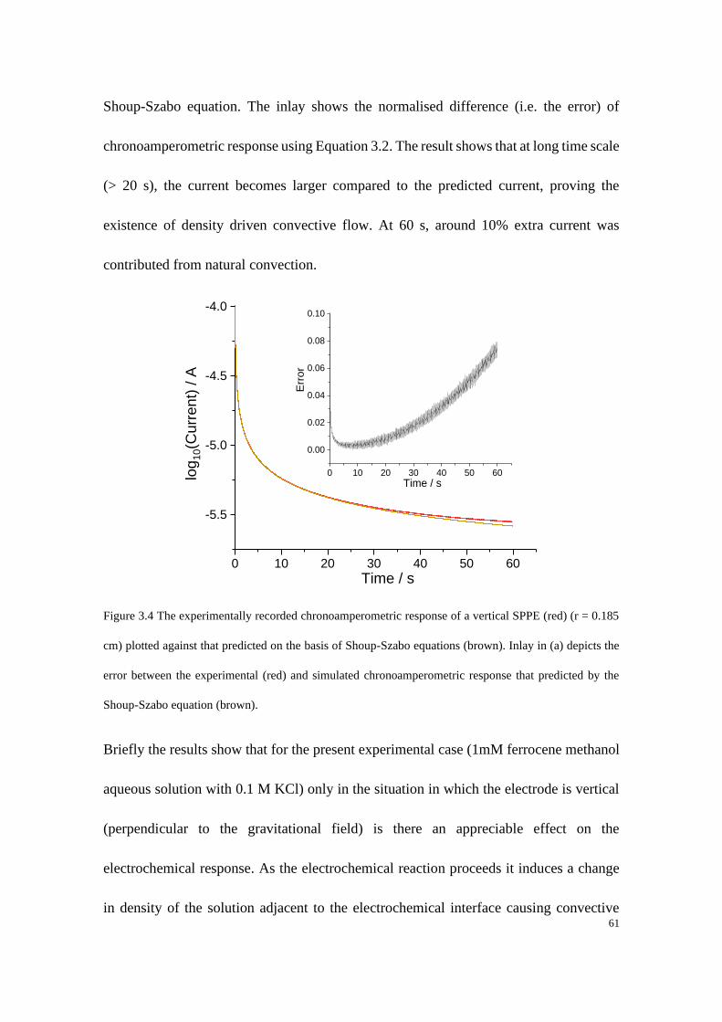
61
Shoup-Szabo equation. The inlay shows the normalised difference (i.e. the error) of
chronoamperometric response using Equation 3.2. The result shows that at long time scale
(> 20 s), the current becomes larger compared to the predicted current, proving the
existence of density driven convective flow. At 60 s, around 10% extra current was
contributed from natural convection.
Figure 3.4 The experimentally recorded chronoamperometric response of a vertical SPPE (red) (r = 0.185
cm) plotted against that predicted on the basis of Shoup-Szabo equations (brown). Inlay in (a) depicts the
error between the experimental (red) and simulated chronoamperometric response that predicted by the
Shoup-Szabo equation (brown).
Briefly the results show that for the present experimental case (1mM ferrocene methanol
aqueous solution with 0.1 M KCl) only in the situation in which the electrode is vertical
(perpendicular to the gravitational field) is there an appreciable effect on the
electrochemical response. As the electrochemical reaction proceeds it induces a change
in density of the solution adjacent to the electrochemical interface causing convective
0 10 20 30 40 50 60
-5.5
-5.0
-4.5
-4.0
0 10 20 30 40 50 60
0.00
0.02
0.04
0.06
0.08
0.10
Err
or
Time / s
log
10(C
urr
ent)
/ A
Time / s
62
flows. In the case of a vertically orientated electrode this results in the mass-transport
limited current being 10% greater than predicted current on the basis of Shoup-Szabo
equation[14]. The influence of such electrochemical reaction induced convection will
lessen as the size of the electrode decreases[9]. Consequently, the above 10% increase in
current for a vertically orientated macroelectrode represents, in this work, a likely largest
possible contribution for natural convection induced by the occurrence of the interfacial
reaction. Hence, in the remainder of this work we continue by only considering the
voltammetric contribution associated with bulk convection arising from thermal
differences in the cell.
3.3.2 Evaporation effects on the voltammetric behaviour of a microcylinder
electrode
We now turn to use a less ‘conventional’ electrode design; that of a micro-cylinder
electrode. The reason for this choice will be evidenced below. Figure 3.5 presents the
voltammetric response of carbon fibre microcylinder electrode (diameter = 7.0 μm and
length 0.961 mm) towards the oxidation of ferrocenemethanol (1 mM) at a scan rate of
25 mV s-1 in both closed (Figure 3.5(a)) and open (Figure 3.5 (b)) cells. The microcylinder
electrode is an interesting geometry for voltammetric experiments where, as is the case
for band electrodes, due to the electrode being macroscopic in one dimension under
diffusion only conditions the voltammogram does not reach a true steady state flux and
in the mass-transport limit the current varies with the inverse of logarithmic time; this
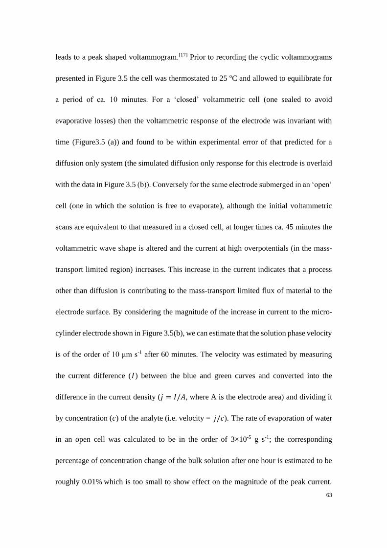
63
leads to a peak shaped voltammogram.[17] Prior to recording the cyclic voltammograms
presented in Figure 3.5 the cell was thermostated to 25 oC and allowed to equilibrate for
a period of ca. 10 minutes. For a ‘closed’ voltammetric cell (one sealed to avoid
evaporative losses) then the voltammetric response of the electrode was invariant with
time (Figure3.5 (a)) and found to be within experimental error of that predicted for a
diffusion only system (the simulated diffusion only response for this electrode is overlaid
with the data in Figure 3.5 (b)). Conversely for the same electrode submerged in an ‘open’
cell (one in which the solution is free to evaporate), although the initial voltammetric
scans are equivalent to that measured in a closed cell, at longer times ca. 45 minutes the
voltammetric wave shape is altered and the current at high overpotentials (in the mass-
transport limited region) increases. This increase in the current indicates that a process
other than diffusion is contributing to the mass-transport limited flux of material to the
electrode surface. By considering the magnitude of the increase in current to the micro-
cylinder electrode shown in Figure 3.5(b), we can estimate that the solution phase velocity
is of the order of 10 μm s-1 after 60 minutes. The velocity was estimated by measuring
the current difference (𝐼) between the blue and green curves and converted into the
difference in the current density (𝑗 = 𝐼/𝐴, where A is the electrode area) and dividing it
by concentration (𝑐) of the analyte (i.e. velocity = 𝑗/𝑐). The rate of evaporation of water
in an open cell was calculated to be in the order of 3×10⁻⁵ g s-1; the corresponding
percentage of concentration change of the bulk solution after one hour is estimated to be
roughly 0.01% which is too small to show effect on the magnitude of the peak current.
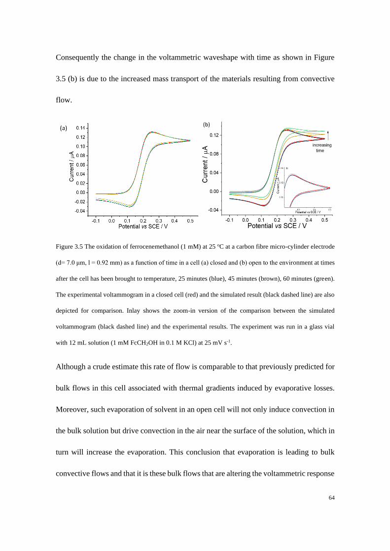
64
Consequently the change in the voltammetric waveshape with time as shown in Figure
3.5 (b) is due to the increased mass transport of the materials resulting from convective
flow.
Figure 3.5 The oxidation of ferrocenemethanol (1 mM) at 25 oC at a carbon fibre micro-cylinder electrode
(d= 7.0 μm, l = 0.92 mm) as a function of time in a cell (a) closed and (b) open to the environment at times
after the cell has been brought to temperature, 25 minutes (blue), 45 minutes (brown), 60 minutes (green).
The experimental voltammogram in a closed cell (red) and the simulated result (black dashed line) are also
depicted for comparison. Inlay shows the zoom-in version of the comparison between the simulated
voltammogram (black dashed line) and the experimental results. The experiment was run in a glass vial
with 12 mL solution (1 mM FcCH2OH in 0.1 M KCl) at 25 mV s-1.
Although a crude estimate this rate of flow is comparable to that previously predicted for
bulk flows in this cell associated with thermal gradients induced by evaporative losses.
Moreover, such evaporation of solvent in an open cell will not only induce convection in
the bulk solution but drive convection in the air near the surface of the solution, which in
turn will increase the evaporation. This conclusion that evaporation is leading to bulk
convective flows and that it is these bulk flows that are altering the voltammetric response
65
is evidenced by the fact that the change in the voltammetric response is only observed
when the cell is open to the environment. Consequently, we conclude that evaporative
losses and the possible induced air movement above the surface of the solution from a
cell can significantly influence the voltammetric response by changing the mass transport.
A closed cell is suggested to be used in experiments to minimise such evaporation effect
(but only once the vapour pressure above the solution reaches the saturated vapour
pressure at 25oC) and meanwhile to suppress any air movement above the solution.
3.3.3 Vibration effects on the voltammetric behaviour of a microcylinder electrode
The optimised thermostated electrochemical cell was used throughout the
experiment to minimised the temperature difference between the normal water bath
and the solution in the cell. In a conventional cell system the electrochemical cell is
held in the water bath using a laboratory clamp held by a clamp stand in a Faraday cage;
consequently the possible vibration of the clamp may be induced by putting the working
electrode into the solution just before the measurement or the closure of the door of the
Faraday cage, which may induce the external convection to the solution and further
induce mechanical movement of the electrode during the measurement. Figure 3.6 shows
how the voltammetric response varies with time in both cell conditions; the comparison
between the experimental and simulated voltammograms is shown in Figure 3.7.
These results show that at short times in the conventional electrochemical system the
microcylinder electrode exhibits a near steady state response (Figure 3.6 (a) red line),

66
over time (ca. minutes) the system stabilises towards a more peaked and hence more
diffusional response. This behaviour is interpreted on the likely basis of the cell not being
held fully rigidly in place despite being ‘clamped’ and as time goes on the vibration of
the cell or the effect of vibration decreases minimising the magnitude of the convective
contribution to the measured Faradaic current at high overpotentials. It is important to
note that in this cell design where a water bath has been used to control the temperature
the voltammetric response, even at long times, does not become purely diffusional as
evidenced through comparison of the voltammetric waveshape with that predicted by
numerical simulation (DigiSim; see experimental section) as shown in Figure 3.7.
Figure 3.6 The oxidation of ferrocenemethanol (1 mM) at 25oC at a carbon fibre microcylinder electrode
(r=3.5 μm, l=0.916 mm) as a function of time in a closed cell in (a) conventional water bath system (clamp
stand) and (b) optimised thermostated electrochemical cell at 25 mV s-1. In Figure (a), the red, magenta and
gray curves represent the voltammograms at the time of 0 s, 600 s and 1200 s respectively. In figure (b),
blue, cyan and black curves represent the voltammograms at the time of 0 s, 600 s and 1200 s respectively.
-0.1 0.0 0.1 0.2 0.3 0.4 0.5-0.04
-0.02
0.00
0.02
0.04
0.06
0.08
0.10
0.12
0.14
0.16
CVs on F8 electrode as a function of time in water bath
Cu
rrent /
A
Potential vs SCE / V
(a)
-0.1 0.0 0.1 0.2 0.3 0.4 0.5
-0.04
-0.02
0.00
0.02
0.04
0.06
0.08
0.10
0.12
0.14
CVs on F8 electrode as a function of time in homemade potentiostat
Cu
rrent /
A
Potential vs SCE / V
(b)
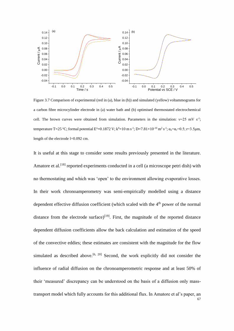
67
Figure 3.7 Comparison of experimental (red in (a), blue in (b)) and simulated (yellow) voltammograms for
a carbon fibre microcylinder electrode in (a) water bath and (b) optimised thermostated electrochemical
cell. The brown curves were obtained from simulation. Parameters in the simulation: ν=25 mV s-1;
temperature T=25 oC; formal potential Eo=0.1872 V; k0=10 m s-1; D=7.81×10⁻¹⁰ m2 s-1; αa=αc=0.5; r=3.5μm,
length of the electrode l=0.092 cm.
It is useful at this stage to consider some results previously presented in the literature.
Amatore et al.[18] reported experiments conducted in a cell (a microscope petri dish) with
no thermostating and which was ‘open’ to the environment allowing evaporative losses.
In their work chronoamperometry was semi-empirically modelled using a distance
dependent effective diffusion coefficient (which scaled with the 4th power of the normal
distance from the electrode surface)[19]. First, the magnitude of the reported distance
dependent diffusion coefficients allow the back calculation and estimation of the speed
of the convective eddies; these estimates are consistent with the magnitude for the flow
simulated as described above.[6, 20] Second, the work explicitly did not consider the
influence of radial diffusion on the chronoamperometric response and at least 50% of
their ‘measured’ discrepancy can be understood on the basis of a diffusion only mass-
transport model which fully accounts for this additional flux. In Amatore et al’s paper, an
-0.1 0.0 0.1 0.2 0.3 0.4 0.5
-0.04
-0.02
0.00
0.02
0.04
0.06
0.08
0.10
0.12
0.14
Cu
rre
nt
/
A
Time / s
Experimental and simulated CVs at CF electrode (F8) at 298 K
(a)
-0.1 0.0 0.1 0.2 0.3 0.4 0.5
-0.04
-0.02
0.00
0.02
0.04
0.06
0.08
0.10
0.12
0.14
Experimental and simulated CVs at CF electrode (F8) at 298 K
Cu
rrent /
A
Potential vs SCE / V
(b)
68
elliptic Pt disk of 1.2 mm equivalent diameter obtained from the slant cross-section (45o)
of a 1 mm diameter platinum wire was used.[21] Here we use a ‘elliptic disk’ model
adapted from Dudko et al’s paper[22] to predict the chronoamperometric response. These
results should be compared to Figure 4 in Amatore’s paper[23], the difference between the
theoretical (with radial diffusion) and Cottrellian chronoamperometric responses in
Figure 3.8 (below) shows that the radial diffusion is likely important in their experimental
setup and should have been considered. These results indicate that at least 50% of their
measured current discrepancy can be understood in terms of the radial diffusion
contribution. However, we speculate the remaining ‘missing’ current may be due to a)
evaporative losses causing bulk fluid motion b) electrode vibrations or c) ‘spontaneous’
convection as defined by Levich i.e. convection arising due to density changes associated
with the occurrence of the electrochemical reaction. We note that Amatore et al. do
discuss the latter point but do not provide evidence that such convection is not operative.
69
Figure 3.8 The comparison between the predicted chronoamperometric response from (blue) Cottrell
equation and (red) the ‘elliptic disk’ equation taken from Dudko et al’s paper[22]. All parameters used were
the same as those in Amatore et al’s paper: D(Fe(CN)64-) = (5.7 ± 0.5) × 10-10 m2 s-1, concentration c = 10
mM.
Further work in the literature[23] suggests that beyond forced and density (aka
gravitationally) driven convection an additional microscopic convection model needs to
be considered to understand natural convection in electrochemical systems. We note
however that first, “a spontaneous excitation of internal convection cannot be generated
from a state at rest in a system which is at thermodynamic equilibrium”,[24] the
‘spontaneous’ natural convection discussed by Levich[5] arises due to the occurrence of
an electrochemical reaction (i.e. it is induced by the system being in a non-equilibrium
state). Moreover, the experimental results we present in Figure 3.2 clearly demonstrate
that for the electrode orientation used relative to the gravitational field (downward),
analyte identity and concentration and, where external influences such as vibrations and
non-perfect thermostating have been minimised, then over a timeframe of 60 seconds at
0 10 20 30 400
5
10
15
20
Curr
ent /
A
Time / s
70
a macro-electrode, no other mass-transport mechanism need be invoked to explain the
results. Furthermore nor do distance dependence diffusion coefficients represent physical
reality but merely attempt to parameterise the transition from stagnant to density driven
convection zone. The results shown in Figure 3.5 demonstrate how convection can be
induced to occur, due to the influence of the external environment on the cell causing
evaporative losses.
It is on the basis of such literature experiments[18a, 23] into convection that a categorisation
of electrodes as either being ‘microelectrodes’ or ‘ultra-microelectrodes’ has been
previously proposed.[21] Zonal diagrams were produced to reportedly define the behaviour
of an electrochemical system. Succinctly it was suggested that larger electrodes are more
sensitive (in terms of their measured voltammetric response) towards natural convection
than smaller ones. Here we ask, to what extent is this generally true?
3.3.4 Effect of natural convection on different electrode geometries
In order to reproducibly and controllably create a density gradient in the electrochemical
cell the system was first thermostated and allowed to equilibrate. Having attained a near
quiescent system the thermostat temperature was increased by one degree Celsius. In the
present experimental system a Peltier heat pump is used to control the thermostat
temperature. This temperature jump method will necessarily induce convective flows in
the electrochemical cell which are likely of the order of 1 mm s-1.[12] Figure 3.9 presents
the recorded voltammetric response for four different electrode types towards the
71
oxidation of ferrocenemethanol prior to (red line) and immediately after (blue line) the
onset of the temperature jump. Over the course of the voltammetric experiment the
solution phase temperature, as recorded in-situ by a thermocouple, was raised by
approximately one degree Celsius, note however, under these conditions the solution
phase temperature in the cell is heterogeneous. Figure 3.9 a) and b) present the
voltammetric responses for a macroscopic (d = 2.98 mm) and a microscopic (d = 33 μm)
disc electrodes where both electrodes are inlaid in a non-conductive support (support
diameters of 6.0 and 3.5 mm). The voltammetric response of neither electrode is
particularly altered by the change in the systems thermostating or hence the induced
convection. Conversely Figure 3.9 c) and d) depicts the voltammetric response of a carbon
fibre microcylinder electrode and a carbon fibre micro tip electrode. Importantly the
carbon fibre electrode (Figure 3.9 d) is only surrounded by a thin glass sheath (~0.4 μm).
The various electrode geometries used are outlined schematically in Figure 3.9. The
voltammetric responses of both electrodes (c and d) are markedly altered by the change
in the thermostating conditions. Moreover, the increase in the mass-transport limited
current cannot be rationalised in terms of the diffusion coefficient of ferrocenemethanol.
For a one degree Celsius change in the solution temperature the diffusion coefficient of
ferrocenemethanol is only anticipated to increase by ca. 2.5 %.[25]

72
Figure 3.9 Effect of temperature change on the voltammograms for (a) macroelectrode, (b) commercial
carbon microdisc electrode, (c) carbon fibre microcylinder electrode and (d) carbon fibre tip electrode.
Macroelectrode used in (a) is glassy carbon electrode with a diameter of 3 mm. Commercial carbon
microdisc electrode used in (b) is 33 μm in diameter. The carbon fibre used in (c) and (d) are 7 μm in
diameter. The red curves represent for the voltammograms at a constant temperature (20 oC), and the blue
curves represents for the voltammograms at each electrode with a temperature jump. Inlays in each figure
represent the schematic of each electrode. The experiments were run in a glass vial with 12 mL solution (1
mM FcCH2OH in 0.1 M KCl) at 25 mV s-1.
The above results directly point to the importance of the electrode surround in altering
the convective profile near the electrode which influences the mass-transport environment
local to the electrochemical interface. The solution phase velocity at a solid surface is
73
necessarily zero (no slip boundary) and a microelectrode inlaid in a relatively large glass
sheath is essentially shielded from the bulk convective flows. Microelectrodes that are
inlaid in non-conductive glass sheaths are less sensitive to bulk convective flows as
compared to macroelectrodes (that are also inlaid in a non-conductive surface). This
however does not mean that microelectrodes are inherently immune to such flows; it is
the non-conducting support structure that creates a larger stagnant layer adjacent to the
electrochemical interface. The notion of a bulk solution in which there is significant
mixing, promoted by density differences, and which is separated from a surface by a
stagnant diffusion layer is of course the physical basis for the simple Nernst diffusion
layer model dating from 1904.[1] But the above results demonstrate more broadly that this
stagnant layer thickness is sensitive to the local environment; the mass-transport to and
from a point on a non-reactive surface will, in terms of the influence of convection, differ
from that of an isolated point in solution.
It is important to recognise that microelectrodes that are not encased in large insulating
surfaces are routinely used in electrochemical experiments. Such electrodes are often
employed for example as probe electrodes in scanning electrochemical microscopy
(SECM) and other analytical contexts. Consequently, if such ‘unsheathed’
microelectrodes are in bulk solution then depending on the local convective environment
the measured steady-state current may differ significantly from that of a diffusion only
model. This has two potential implications: first, the accurate calibration of such
electrodes may be challenging; second, in experimental setups where the electrodes

74
distance from an interface is varied, such as an approach curve, the influence of
convection on the measured electrochemical response will vary as a function of the
electrode/surface separation. Therefore, the careful and rigorous[26] thermostating of
electrochemical systems using such unsheathed microelectrodes is a likely necessary
requisite.
In summary, convection in electrochemical systems can significantly influence the
voltammetric response. Generally convection is classified as either forced or natural.
Forced convection induced by deliberate flowing, vibrating or rotating of the electrode is
a routinely used method to enhance the rate of mass-transport to an electrochemical
interface. However, in the absence of deliberately induced convection it is common for
an electrochemical system to be interpreted solely on the basis of a diffusion-only model.
However, there are a number of mechanisms that may still lead to the convective
movement of the solution in an electrochemical cell. First, there may be sources of
external adventitious forced convection, a prime example being vibrations arising from
the laboratory environment. Such unintentional sources of forced convection can be, as
is done in this work, often easily and sufficiently minimised by firmly securing the cell
and damping local vibration sources. More complex is the issue of so-called natural
convection. Natural convection is a broad term encompassing a number of physical
phenomena. Generally natural convection refers to gravitationally driven convection
resulting from local density differences in the solution. As outlined by Levich[5] such
density differences may be driven by the occurrence of the electrochemical reaction itself,
75
arising either due to the reaction enthalpy or molar volume change associated with the
electrochemical reaction.
3.4 Conclusions
In this work we use low (millimolar) concentrations of the electroactive analyte and
demonstrate experimentally that for the orientation (horizontally facing downward) of the
electrode the influence of natural convection induced by the change in enthalpy or the
reaction molar volume of the electrochemical reaction itself only contributes minimally
to the observed voltammetry. Consequently, having minimised and controlled all other
sources of forced and natural convection this allows us to investigate to what extent
thermally induced natural convection can be important in such voltammetric
measurements. We demonstrate how imperfect thermostating of an electrochemical cell
can and does lead to significant density driven convective flows. These convective flows
may influence an electrochemical response of a system by altering the mass-transport
regime. This convection can be driven simply by the evaporative loss of solution from an
electrochemical cell which is open to the environment. The use of distance dependent
diffusion coefficients to model the effects of convection in an electrochemical cell, as
employed in the literature, is cautioned against on conceptual, theoretical[24] and
experimental bases.
Importantly, we show how the sensitivity of an electrode towards convective flows in the
bulk solution is not just a function of the electrodes size but is also importantly influenced
76
by the size and geometry of the non-conductive support surrounding the electrode. The
sensitivity of a microelectrode towards bulk convective flows is less if the electrode is
inlaid into a large macroscopic surface. The surrounding substrate serves to shield the
electrode and creates a larger stagnant layer near the reactive interface. This highlights a
general insight that unsheathed microelectrodes i.e. ones that are not embedded in a large
non-conductive support surface are generally more sensitive to solution phase convection.
This has potential implications for a variety of experimental systems that used such
unsheathed electrodes; highlighting a source of irreproducibility that is generally not
considered.
References:
[1] W. Nernst, Z. Phys. Chem. 1904, 47U, 52.
[2] D. Li, C. Batchelor-McAuley, L. Chen, R. G. Compton, Physical Chemistry Chemical Physics
2019, 21, 9969-9974.
[3] R. G. Compton, C. E. Banks, Understanding Voltammetry, 3rd ed., World Scientific Publishing
Company Pte Limited, 2018.
[4] Á. Molina, J. González, Pulse Voltammetry in Physical Electrochemistry and Electroanalysis:
Theory and Applications, Springer International Publishing, 2015.
[5] V. G. Levich, Physicochemical Hydrodynamics: (by) Veniamin G. Levich. Transl. by Scripta
Technica, Inc, Prentice-Hall, 1962.
[6] J. K. Novev, S. Eloul, R. G. Compton, J. Phys. Chem. C 2016, 120, 13549-13562.
[7] aG.-U. Flechsig, Curr. Opin. in Electrochem. 2018, 10, 54-60; bP. Gründler, In-situ
Thermoelectrochemistry: Working with Heated Electrodes, Springer Berlin Heidelberg, 2015; cP.
Gründler, D. Degenring, J. Electroanal. Chem. 2001, 512, 74-82; dP. Gründler, G.-U. Flechsig,
Microchimica Acta 2006, 154, 175-189; eP. Gründler, T. Zerihun, A. Möller, A. Kirbs, J.
Electroanal. Chem. 1993, 360, 309-314; fA. S. Baranski, Anal. Chem. 2002, 74, 1294-1301; gF.
Marken, Y.-C. Tsai, B. A. Coles, S. L. Matthews, R. G. Compton, New J. Chem. 2000, 24, 653-
658; hA. Boika, A. S. Baranski, Anal. Chem. 2008, 80, 7392-7400; iJ. Wang, P. Gründler, G.-U.
Flechsig, M. Jasinski, G. Rivas, E. Sahlin, J. L. Lopez Paz, Anal. Chem. 2000, 72, 3752-3756.
[8] K. Ngamchuea, S. Eloul, K. Tschulik, R. G. Compton, Anal. Chem. 2015, 87, 7226-7234.
[9] X. Gao, J. Lee, H. S. White, Anal. Chem. 1995, 67, 1541-1545.

77
[10] T. M. Squires, M. Z. Bazant, J. Fluid Mech. 2004, 509, 217-252.
[11] aJ. K. Novev, R. G. Compton, Phys. Chem. Chem. Phys. 2017, 19, 12759-12775; bJ. K. Novev,
R. G. Compton, Phys. Chem. Chem. Phys. 2016, 18, 29836-29846.
[12] X. Li, C. Batchelor-McAuley, J. K. Novev, R. G. Compton, Phys. Chem. Chem. Phys. 2018, 20,
11794-11804.
[13] aM. Rudolph, J. Electroanal. Chem. Interfacial Electrochem. 1991, 314, 13-22; bM. Rudolph, J.
Electroanal. Chem. 1992, 338, 85-98; cM. Rudolph, J. Electroanal. Chem. 1994, 375, 89-99.
[14] D. Shoup, A. Szabo, J. Electroanal. Chem. Interfacial Electrochem. 1982, 140, 237-245.
[15] K. Ngamchuea, C. Lin, C. Batchelor-McAuley, R. G. Compton, Anal. Chem. 2017, 89, 3780-3786.
[16] R. G. Compton, E. L. Laborda, K. R. Ward, Understanding Voltammetry: Simulation Of Electrode
Processes, World Scientific Publishing Company, 2013.
[17] A. J. Bard, L. R. Faulkner, Electrochemical Methods: Fundamentals and Applications, 2nd
Edition, John Wiley & Sons, 2000.
[18] aC. Amatore, S. Szunerits, L. Thouin, J. S. Warkocz, Electroanalysis: An International Journal
Devoted to Fundamental and Practical Aspects of Electroanalysis 2001, 13, 646-652; bN. Baltes,
L. Thouin, C. Amatore, J. Heinze, Angewandte Chemie International Edition 2004, 43, 1431-1435.
[19] A questionable consequence of this approach is that diffusion coefficients measured
electrochemically may not quantitatively agree with those made by other 'bulk' measurement
techniques such as conductance.
[20] J. K. Novev, R. G. Compton, Curr. Opin. in Electrochem. 2018, 7, 118-129.
[21] C. Amatore, C. c. Pebay, L. Thouin, A. Wang, J. S. Warkocz, Analytical chemistry 2010, 82, 6933-
6939.
[22] O. K. Dudko, A. Szabo, J. Ketter, R. M. Wightman, Journal of Electroanalytical Chemistry 2006,
586, 18-22.
[23] C. Amatore, S. Szunerits, L. Thouin, J.-S. Warkocz, J. Electroanal. Chem. 2001, 500, 62-70.
[24] P. Glansdorff, I. Prigogine, Thermodynamic Theory of Structure, Stability and Fluctuations, Wiley,
1971.
[25] The diffusion coefficient is inversely proportional to the dynamic viscosity of the liquid. The
percentage difference in diffusion coefficient was calculated using the inverse ratio of viscosity of
water at 20 degree Celsius to viscosity at 21 degree Celsius.
[26] D. Schäfer, A. Puschhof, W. Schuhmann, Phys. Chem. Chem. Phys. 2013, 15, 5215-5223.
78
Chapter 4
Tafel Analysis under Different Electrode Geometries
Tafel analysis is a basic and powerful tool to extract kinetic information from measured
voltammograms. In this chapter voltammetric waves under five different mass-transport
regimes (macroelectrode, microdisc, micro-hemisphere, micro-hemicylinder and single
microband) for an irreversible one electron transfer process were simulated and analysed
to find the appropriate Tafel region for accurate analysis. The transfer coefficient was
found to deviate significantly from its true value as a function of potential in all cases due
to the influence of mass-transport. If and how a simple analytical mass-transport
correction in which the current is corrected for the change in the reactant concentration at
the surface can be used to improve the measurement of transfer coefficient were
investigated. It is shown that this correction is only rigorously valid for a uniformly
accessible microelectrode under a true steady-state condition. This translates to
hemispherical electrodes only of the set of five considered. The fraction of the current
used in Tafel analysis (Tafel region) can be increased to around 50% for quasi-steady
state regimes (hemi-cylindrical and single band electrodes) with this analytical correction
but it completely failed in linear diffusion regimes (macroelectrodes). In the latter case
an improved empirical correction is suggested.
79
This work presented in this chapter has been published as a first author paper in Journal
of Electroanalytical Chemistry[1] and was carried out in collaboration with Dr. Chuhong
Lin, Dr. Christopher Batchelor-McAuley and Mr. Lifu Chen.
4.1 Introduction
Voltammetric experiments can yield significant thermodynamic and kinetic
information.[2] However, due to the convolution of the time and energy domains
extraction of this data is often non-facile. In many cases measurement of the related
physico-chemical parameters may only be fully achieved through simulation of the
system. Notwithstanding this, due in part for ease and expediency, it is very common for
voltammetric experiments to be analysed using mathematically analytical procedures. Of
these analytical methods, Tafel analysis is a cornerstone of the electrochemist’s tool box.
Tafel analysis of a voltammogram yields a measure of the electrochemical system’s
transfer coefficient[3]. First, under appropriate conditions, the transfer coefficient can
provide information regarding the electrochemical mechanism[4]. Classically, Tafel
analysis has been used to great effect in the analysis and elucidation of the catalytic
activity of various metal surfaces towards the hydrogen evolution reaction[5]. Second, for
irreversible voltammetry at a macroelectrode (linear diffusion regime) the transfer
coefficient needs to be known in order for the species diffusion coefficient to be
accurately determined[6].
80
The transfer coefficient is a dimensionless parameter and describes how the rate of an
interfacial oxidation or reduction reaction varies as a function of the applied potential,
under the caveat that the concentration of the reactant at the electrode surface is unaltered
from its value in bulk solution. The physical interpretation of the transfer coefficient is
often dependent upon the assumption of an underlying electrochemical mechanism.
Moreover, for electrochemical processes involving the transfer of multiple electrons
and/or the formation and breaking of chemical bonds (i.e. processes comprised of
multiple sequential elementary steps) the interpretation of the transfer coefficient is not
straightforward[7]. However, for a simple and single electron transfer process the transfer
coefficient is commonly qualitatively interpreted being a measure of the ‘position’ of the
transition state[6], where a transfer coefficient close to unity implies the transition state is
‘reactant-like’ and similarly a value close to zero implies a ‘product-like’ transition state
for an oxidative process.
The Butler-Volmer equation is a phenomenological description of the rate of an
interfacial redox reaction where the reaction rate increases exponentially as a function of
the applied potential. In this framework it is commonly assumed that the transfer
coefficient is a constant and independent of the applied potential. In contrast Marcus-
Hush theory[8] provides a microscopic model of an interfacial electron transfer process,
here the rate of the reaction is rationalised in terms of the reaction Gibbs energy and a
reorganisation energy[9]. The reorganisation energy is related to the energy required to
distort the reactant molecule and its solvation shell to those of the product. Commonly,
81
the force constants for the reduced and oxidised species are assumed to be equal
(symmetric): this is equivalent to assuming that at low overpotentials that the transfer
coefficient has a value of 0.5. However, even for many apparently outer-sphere redox
processes the transfer coefficient is found to deviate from 0.5[10]. Relaxation of the
assumption of equal force constants, allows (asymmetric) Marcus-Hush theory to be
reconciled with the Butler-Volmer equation[11]. The latter can be viewed as a good
approximation of the former at low overpotentials and the transfer coefficient can be
quantitatively interpreted as reflecting the asymmetry in the force constants for the
reduced and oxidised species.
For both the symmetric and asymmetric forms of Marcus-Hush theory, these microscopic
theories predict a deviation of the reaction rate from exponentially increase at high
overpotentials; ultimately the rate becomes independent of the applied potential,
becoming mass-transport controlled. The predicted deviation away from exponentially
increasing reaction rate may be expressed as a potential dependent transfer coefficient (or
equivalently as a ‘curved’ Tafel slope). The experimental reporting of such curved Tafel
slopes and potential dependent transfer coefficients have historically[12] played an
important role in validating and advancing our physical insight into this class of
heterogeneous reactions. However, during the course of a voltammogram the reactant
rapidly becomes depleted at the electrode surface and the rate determining step becomes
the mass-transport of material to the electrode surface. Consequently, before interpreting
an experimental Tafel plot and the associated transfer coefficient it is important to
82
quantify over what range of voltammetric currents can the voltammogram be directly
analysed within the Butler-Volmer approach to yield an accurate measure of the transfer
coefficient? A further issue is to what extent can the depletion of the reactant be corrected
for using analytical approximations? The present work in this chapter addresses and
answers these two questions.
4.2 Background theory
4.2.1 Butler-Volmer kinetics
We consider the following one electron transfer oxidative process under different mass-
transport geometries:
A ⇄ B + 𝑒− (4.1)
where the reactant and product in the process are assumed to have equal diffusion
coefficients with only reactant present in bulk solution.
Butler-Volmer (BV) theory is experimentally the most commonly used kinetic model.[13]
According to BV theory, the oxidative and reductive rate constants (𝑘𝑎, 𝑘𝑐) are functions
of the transfer coefficients, the standard rate constant 𝑘0 and the formal potential 𝐸𝑓0[6]:
𝑘𝑎 = 𝑘0𝑒𝑥𝑝[𝛼𝑎,𝐵𝑉𝜃] (4.2)
𝑘𝑐 = 𝑘0𝑒𝑥𝑝[−𝛼𝑐,𝐵𝑉𝜃] (4.3)
83
where the anodic transfer coefficient 𝛼𝑎,𝐵𝑉 and the cathodic transfer coefficient 𝛼𝑐,𝐵𝑉
are between 0 and 1, 𝛼𝑎,𝐵𝑉 + 𝛼𝑐,𝐵𝑉 = 1, and θ is the dimensionless potential given by:
𝜃 =𝐹
𝑅𝑇(𝐸 − 𝐸𝑓
0) (4.4)
where E is the potential of the working electrode, F is the Faraday constant (96485 C mol-
1), R is the gas constant (8.314 J mol-1 K-1) and T is the temperature in K. 𝛼𝑎,𝐵𝑉 and
𝛼𝑐,𝐵𝑉 are commonly assumed to be independent of potential.
4.2.2 Tafel analysis
The International Union of Pure and Applied Chemistry (IUPAC) formally defines the
anodic and cathodic transfer coefficients as being experimentally determined values and
given by[3]:
𝛼𝑎 =𝑅𝑇
𝐹(
𝑑𝑙𝑛𝑗𝑎,𝑐𝑜𝑟𝑟
𝑑𝐸) (4.5)
𝛼𝑐 = −𝑅𝑇
𝐹(
𝑑𝑙𝑛|𝑗𝑐,𝑐𝑜𝑟𝑟|
𝑑𝐸) (4.6)
where 𝑗𝑎,𝑐𝑜𝑟𝑟 and 𝑗𝑐,𝑐𝑜𝑟𝑟 are the anodic and cathodic current densities corrected for any
changes in the reactant concentration at the electrode surface with respect to its bulk value.
The definitions avoid the need for any knowledge of the overall number of electrons
transferred.
If a process is considered to be fully irreversible, for an oxidative process, when the
applied potential is sufficiently far from the equilibrium potential Eeq, it is possible to
84
neglect the flux contribution from the reduction. Hence, the electrochemical flux can be
expressed as:
𝑗𝑎 = 𝑘𝑎[𝐴]0 = 𝑘0𝑒𝑥𝑝 [𝛼𝑎𝐹(𝐸−𝐸𝑓)
𝑅𝑇] [𝐴]0 (4.7)
where 𝑗𝑎 is the experimentally measured anodic flux density and [𝐴]0 is the
concentration of the reactant at the electrode surface, which is typically different from
that in bulk solution except close to the ‘foot’ of the voltammetric wave. Due to the
sensitivity of 𝑗𝑎 to [𝐴]0, surface depletion of the reactant inherently leads to a mass-
transport limitation of the measured current.
This anodic electrochemical flux 𝐼𝑎 can be directly related to the measured current by:
𝐼𝑎 = ∫ 𝐹𝑗𝑎𝑑𝐴 (4.8)
By combining Equations 4.7 and 4.8, rearranging and assuming the flux is uniform across
the electrode surface, we get the expression:
ln|𝐼𝑎| =𝛼𝑎𝐹(𝐸−𝐸𝑓
0)
𝑅𝑇+ 𝑙𝑛(𝐹𝐴𝑘0[𝐴]0) (4.9)
Consequently, if [𝐴]0 does not deviate significantly from its bulk value, a plot of ln|𝐼𝑎|
versus 𝐸 yields a straight line with a gradient proportional to 𝛼𝑎. Hence plots of ln|𝐼|
versus 𝐸 are commonly used to extract the transfer coefficient from voltammetric data
and are referred to as ‘Tafel plots’. The resulting line of best fit will yield a measure of
the transfer coefficient averaged over a range of potentials. However, mirroring the

85
IUPAC recommendations, if the plot is curved, the transfer coefficient can be defined as
a function of potential.
Problematically, implementation of Equations 4.5 and 4.6 requires precise knowledge of
the mass-transport regime to allow the flux to be suitably corrected for deviations in the
surface concentration of the reactant. Consequently, for expediency and/or due to the lack
of knowledge regarding the nature of the mass-transport regime (in contrast to Equations
4.5 and 4.6), the experimentally accessible parameters are:
𝑅𝑇
𝐹
𝑑𝑙𝑛𝐼𝑎
𝑑𝐸= 𝛼𝑎,𝑛𝑐 (4.10)
−𝑅𝑇
𝐹
𝑑𝑙𝑛|𝐼𝑐|
𝑑𝐸= 𝛼𝑐,𝑛𝑐 (4.11)
where 𝐼𝑐 is the experimentally measured cathodic current, 𝛼𝑎,𝑛𝑐 and 𝛼𝑐,𝑛𝑐 are the non-
mass-transport corrected or ‘apparent’ transfer coefficients. The transfer coefficient 𝛼𝑛𝑐
may deviate from its true value 𝛼𝑎 due to the local depletion of reagents at the
electrochemical interface. However, at low current densities (i.e. 𝐼 → 0), 𝛼𝑛𝑐 → 𝛼.
It is useful to comment that Tafel plots (ln|𝐼| versus E) as used in this work differ from
its historical form (overpotential η versus 𝑙𝑜𝑔10𝐼 ) as measured from galvanostatic
experiments. The classically defined Tafel slope with the unit as mV per decade of current
is directly related to the transfer coefficient (𝑇𝑎𝑓𝑒𝑙 𝑠𝑙𝑜𝑝𝑒 = 2.3𝑅𝑇/𝛼𝑎𝐹). For example,
𝛼𝑎 = 0.5 is equivalent to the Tafel slope of ca. 118 mV per decade. In this work,
potentiostatic control is assumed, and consequently it is appropriate to define the Tafel
plot as ln|𝐼| versus E, the slope of which is proportional to the transfer coefficient.
86
4.2.3 Mass-transport corrected Tafel analysis
Correction of the current or flux to account for the change in the reactant concentration
at the surface requires knowledge of the mass-transport regime. Such corrections may be
achieved through numerical simulation using the experimentally measured current as a
boundary condition[2b]. However, it is far more common to use an analytical expression
to provide an approximate mass-transport correction[6, 14].
The analytical expression is based on the assumption of a uniformly accessible
microelectrode, where a true steady state can be attained after sufficient long time. Under
these conditions, for a fully irreversible electrode process, the flux can be expressed via
the Nernst diffusion layer approximation, where the diffusion layer thickness 𝛿 is often
taken as invariant with time[6, 15] and is:
𝑗𝑎 = 𝐷 ([𝐴]0−[𝐴]𝑏𝑢𝑙𝑘
𝛿) (4.12)
Under BV theory, the analytical expressions describing mass-transport corrected transfer
coefficients 𝛼′ are:
−𝑅𝑇
𝐹
𝑑𝑙𝑛(1
𝐼𝑎−
1
𝐼𝑙𝑖𝑚)
𝑑𝐸= 𝛼𝑎
′ (4.13)
𝑅𝑇
𝐹
𝑑𝑙𝑛|1
𝐼𝑐−
1
𝐼𝑙𝑖𝑚|
𝑑𝐸= 𝛼𝑐
′ (4.14)
where 𝐼𝑙𝑖𝑚 is the mass-transport limiting current and 𝛼𝑎′ and 𝛼𝑐
′ are the measured
analytically mass-transport corrected anodic and cathodic transfer coefficients,
87
respectively. The full deviation of these expressions is presented in the Appendix A
Section A1.
Ideally, 𝛼′ should have the same value as 𝛼 after mass-transport correction. However,
this analytical mass-transport correction as a result of the breakdown of the assumptions
made in its derivation is not applicable in all cases. Therefore, 𝛼′ is considered as an
analytical approximation to the mass-transport corrected transfer coefficient. A linear
relationship of ln |1
𝐼−
1
𝐼𝑙𝑖𝑚| with the dimensionless potential θ is expected when the
assumptions are met.[16] In this work, the extent to which how accurate the analytically
mass-transport corrected Tafel analysis is under different diffusion geometries is studied.
4.3 Numerical simulation procedures
The commercially available simulation software DigiSim® is used to simulate the one-
dimensional (1D) diffusion models. It is based on a fully implicit finite difference (IFD)
algorithm suggested by Manfred Rudolph[17] and it allows simulations for a wide range
of mechanisms.
The voltammetric response on a 2D diffusion microdisc electrode is simulated using a
home-written programme which is based on the conformal mapping of the spatial
coordinates and uses an exponentially expanding time grid.[18]
Although the current at a microband electrode is often approximated by a hemicylinder
of equivalent area (𝑟 = 𝑤/𝜋, where 𝑟 is the radius of the hemicylinder and 𝑤 is the
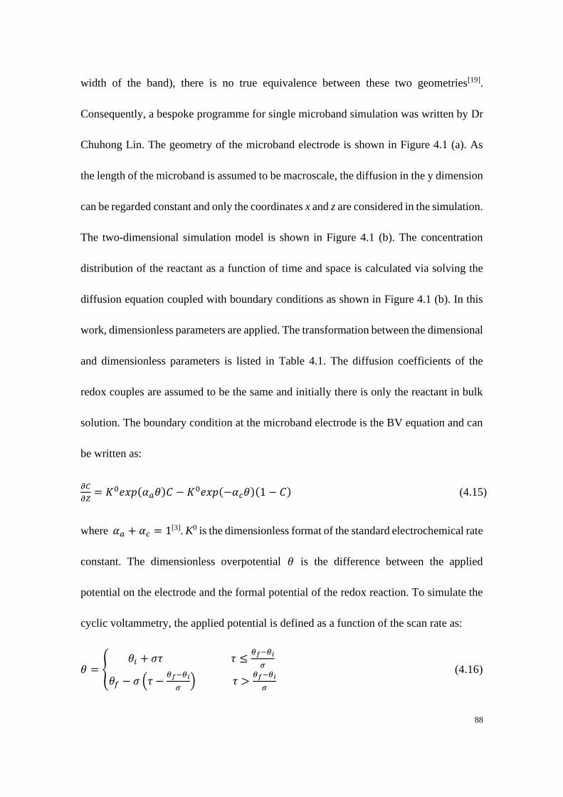
88
width of the band), there is no true equivalence between these two geometries[19].
Consequently, a bespoke programme for single microband simulation was written by Dr
Chuhong Lin. The geometry of the microband electrode is shown in Figure 4.1 (a). As
the length of the microband is assumed to be macroscale, the diffusion in the y dimension
can be regarded constant and only the coordinates x and z are considered in the simulation.
The two-dimensional simulation model is shown in Figure 4.1 (b). The concentration
distribution of the reactant as a function of time and space is calculated via solving the
diffusion equation coupled with boundary conditions as shown in Figure 4.1 (b). In this
work, dimensionless parameters are applied. The transformation between the dimensional
and dimensionless parameters is listed in Table 4.1. The diffusion coefficients of the
redox couples are assumed to be the same and initially there is only the reactant in bulk
solution. The boundary condition at the microband electrode is the BV equation and can
be written as:
𝜕𝐶
𝜕𝑍= 𝐾0𝑒𝑥𝑝(𝛼𝑎𝜃)𝐶 − 𝐾0𝑒𝑥𝑝(−𝛼𝑐𝜃)(1 − 𝐶) (4.15)
where 𝛼𝑎 + 𝛼𝑐 = 1[3]. K0 is the dimensionless format of the standard electrochemical rate
constant. The dimensionless overpotential 𝜃 is the difference between the applied
potential on the electrode and the formal potential of the redox reaction. To simulate the
cyclic voltammetry, the applied potential is defined as a function of the scan rate as:
𝜃 = {𝜃𝑖 + 𝜎𝜏 𝜏 ≤
𝜃𝑓−𝜃𝑖
𝜎
𝜃𝑓 − 𝜎 (𝜏 −𝜃𝑓−𝜃𝑖
𝜎) 𝜏 >
𝜃𝑓−𝜃𝑖
𝜎
(4.16)
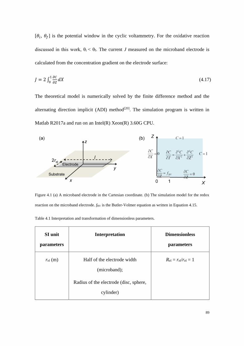
89
[𝜃𝑖, 𝜃𝑓] is the potential window in the cyclic voltammetry. For the oxidative reaction
discussed in this work, θi < θf. The current J measured on the microband electrode is
calculated from the concentration gradient on the electrode surface:
𝐽 = 2 ∫𝜕𝐶
𝜕𝑍
1
0𝑑𝑋 (4.17)
The theoretical model is numerically solved by the finite difference method and the
alternating direction implicit (ADI) method[20]. The simulation program is written in
Matlab R2017a and run on an Intel(R) Xeon(R) 3.60G CPU.
Figure 4.1 (a) A microband electrode in the Cartesian coordinate. (b) The simulation model for the redox
reaction on the microband electrode. fBV is the Butler-Volmer equation as written in Equation 4.15.
Table 4.1 Interpretation and transformation of dimensionless parameters.
SI unit
parameters
Interpretation Dimensionless
parameters
rel (m) Half of the electrode width
(microband);
Radius of the electrode (disc, sphere,
cylinder)
Rel = rel/rel = 1

90
lel (m) Length of the microband
x (m) Space coordinate, parallel to the
electrode surface
X = x/rel
z (m) Space coordinate, perpendicular to the
electrode surface
Z = z/rel
cbulk (mM) Concentration in the bulk solution Cbulk = cbulk/cbulk = 1
c (mM) Concentration C = c/cbulk
D (m2 s-1) Diffusion coefficient d = D/D = 1
t (s) Reaction time τ = t*D/rel2
F (C mol-1) Faraday constant (96485 C mol-1)
R (J⋅mol−1⋅
K−1)
Gas constant (8.314 J⋅mol−1⋅K−1)
T (K) Experiment temperature (298.2 K)
Ef (V) Formal potential
E (V) Applied electrode potential θ= (E - Ef)F/(RT)
k0 (m s-1) Standard electrochemical rate constant K = k0rel/D
v (V s-1) Scan rate σ= vFrel2/(RTD)
I (A) Current J = I/ (FDcbulklel)

91
4.4 Results and discussion
Oxidative voltammograms on different electrode geometries were simulated. The
waveshapes and the non-mass-transport corrected (‘apparent’) transfer coefficient 𝛼𝑛𝑐
as a function of potential were analysed. We first aim to assess over which range of
voltammetric current without mass-transport correction 𝛼𝑛𝑐 closely reflects the true
transfer coefficient 𝛼. Second, the accuracy or otherwise of using the analytical defined
mass-transport correction (Equations 4.13 and 4.14) is investigated.
The process studied in this work is a fully irreversible, one-electron transfer reaction
(Equation 4.1). Five different diffusion geometries, macrodisc, micro-hemispherical,
micro-disc, micro-hemicylindrical and single microband electrodes, are investigated in
this work. Voltammograms on different geometries were simulated using either
DigiSim® or a home-written programme as described above. The analysis presented here
focuses on oxidative processes only, but the results are also equally applicable to the
irreversible reductive processes. The anodic and cathodic transfer coefficients as used in
the BV equation are added to unity except where otherwise stated. All the Tafel analysis
was undertaken in the current range from 1% to 99% of the peak current 𝐼𝑝 or steady-
state current 𝐼𝑠.𝑠. Experimentally, the lower limit percentage of current should be chosen
based on the ratio of faradaic current to background current, this lower limit will vary
between different electrode systems, further details on which are outlined in the

92
discussion presented in Appendix A Section A2. Three mass-transport regimes will be
discussed in the sequence: linear diffusion, steady-state and quasi-steady state.
4.4.1 Electrodes with linear diffusion
4.4.1.1 Tafel analysis under linear diffusion
For a planar disc electrode, both linear and radial (near the electrode edge) diffusion
contribute to the total mass-transport limited flux. However, at sufficiently short times or
for larger electrodes, when the diffusion layer thickness is small as compared to the
electrode radius, only the linear diffusion contribution needs to be considered. The limits
of this linear diffusion regime can be described via the dimensionless scan rate σ (defined
in Table 4.1). When σ is in excess of ca 3350[21] as is commonly encountered when
using a macroelectrode the diffusion to the electrode can be assumed to be linear.
Under these conditions the resulting maximum current is expected to be within
experimental error (no more than 3% greater compared to that predicted for a linear
diffusion regime from Randles-Ševčík equation)[21]. The flux is then considered as
uniform over the electrode surface and results in a peak-shaped cyclic voltammogram.
The simulations were done at the same dimensionless scan rate and dimensionless rate
constant for easy comparison. Here voltammograms on linear diffusion electrodes at
different dimensionless scan rates were simulated using DigiSim®, with the transfer
coefficients αa and αc equal to 0.5 and a dimensionless rate constant K of 1.5×10⁻³. The
93
normalised voltammograms at different dimensionless scan rates (σ = 2.19×10³, 2.19×10⁴
and 2.19×10⁵) were superimposed in Figure 4.2 where the y-axis is the dimensionless
current which was normalised to the peak current and the x-axis is the dimensionless
potential. The results show that in the fully irreversible limit, although the magnitude of
the peak current is proportional to the square root of the scan rate and its position on the
potential scale shifts with the scan rate, the dimensionless voltammetric waveshape is
independent of the dimensionless scan rate. This fully irreversible case is further shown
in Figure 4.3 (a) in the following section.
Figure 4.2 (a) Effect of various dimensionless scan rates on the waveshape under linear diffusion. (b)
Anodic transfer coefficient plot for linear diffusion at different dimensionless scan rates. Red: σ = 2.19×10³;
Blue: σ = 2.19×10⁴; Brown: σ = 2.19 × 10⁵. The dimensionless rate constant K = 1.5 × 10⁻³. Transfer
coefficients αa = αc = 0.5.
Non-mass transport corrected transfer coeffiscient plot The voltammogram simulated
for a dimensionless scan rate of 2.19×10⁴ were selected for Tafel analysis with a
dimensionless rate constant K of 1.5×10⁻³. The results where both the anodic and cathodic
transfer coefficients αa and αc are 0.5 were first presented. Cases where the transfer
94
coefficient does not equal to 0.5 will be later discussed. Figure 4.3(a) shows the
voltammogram normalised relative to the voltammetric peak current. The Tafel plot
(ln|𝐼𝑎| versus θ) was then calculated over the current range of 1% to 99% of the peak
current and is shown in the inlay of Figure 4.3(a). The slope of the Tafel plot corresponds
to the anodic transfer coefficient 𝛼𝑎,𝑛𝑐. It can be seen that the Tafel plot is not a straight
line over the potential range; the value of 𝛼𝑎,𝑛𝑐 is not a constant.
In order to more clearly visualise how the non-mass-transport-corrected anodic transfer
coefficient changes with dimensionless potential θ, the first derivative of the Tafel plot
(Equation 4.10) is presented as the blue curve in Figure 4.3(b). It shows that at very low
current, the measured anodic transfer coefficient 𝛼𝑎,𝑛𝑐 approaches the true value of 0.5,
but deviates from this value at high currents. This deviation occurs due to the depletion
of the reactant at the electrode surface. Upon reaching the peak current the ‘apparent’ or
non-mass-transport corrected transfer coefficient (𝛼𝑎,𝑛𝑐) tends to zero. Moreover, in order
to numerically express how far the measured 𝛼𝑎,𝑛𝑐 deviates from the true value as a
function of potential, the fraction of the oxidative wave that can be used in the Tafel
analysis for a given error has been calculated using Equation 4.18.
𝐸𝑟𝑟𝑜𝑟 𝑖𝑛 𝛼𝑎 =|𝛼𝑎,𝑛𝑐− 𝛼𝑎|
𝛼𝑎× 100% (4.18)
Frequently, up to 50% of the rising part of the voltammogram is taken for Tafel analysis
in order to get rid of the influence from background current and diffusion effect[6, 22].
However, from the results presented in Table 4.2 it can be seen that at 50% of the way up
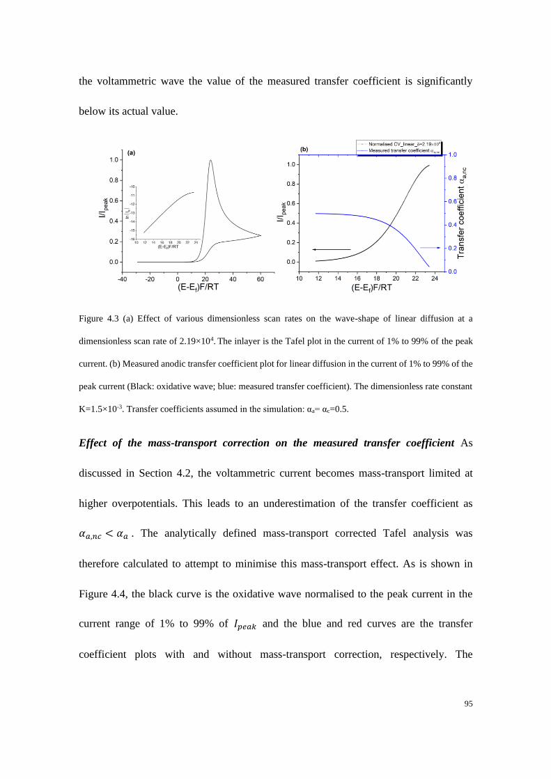
95
the voltammetric wave the value of the measured transfer coefficient is significantly
below its actual value.
Figure 4.3 (a) Effect of various dimensionless scan rates on the wave-shape of linear diffusion at a
dimensionless scan rate of 2.19×10⁴. The inlayer is the Tafel plot in the current of 1% to 99% of the peak
current. (b) Measured anodic transfer coefficient plot for linear diffusion in the current of 1% to 99% of the
peak current (Black: oxidative wave; blue: measured transfer coefficient). The dimensionless rate constant
K=1.5×10⁻³. Transfer coefficients assumed in the simulation: αa= αc=0.5.
Effect of the mass-transport correction on the measured transfer coefficient As
discussed in Section 4.2, the voltammetric current becomes mass-transport limited at
higher overpotentials. This leads to an underestimation of the transfer coefficient as
𝛼𝑎,𝑛𝑐 < 𝛼𝑎 . The analytically defined mass-transport corrected Tafel analysis was
therefore calculated to attempt to minimise this mass-transport effect. As is shown in
Figure 4.4, the black curve is the oxidative wave normalised to the peak current in the
current range of 1% to 99% of 𝐼𝑝𝑒𝑎𝑘 and the blue and red curves are the transfer
coefficient plots with and without mass-transport correction, respectively. The
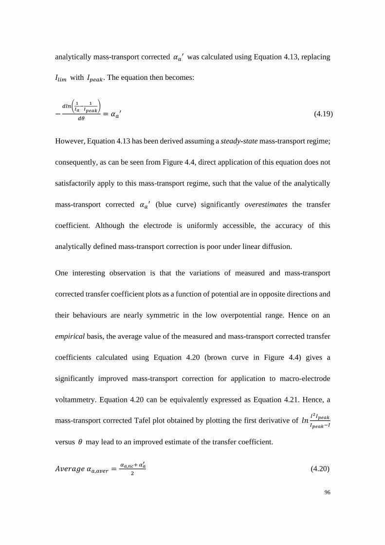
96
analytically mass-transport corrected 𝛼𝑎′ was calculated using Equation 4.13, replacing
𝐼𝑙𝑖𝑚 with 𝐼𝑝𝑒𝑎𝑘. The equation then becomes:
−𝑑𝑙𝑛(
1
𝐼𝑎−
1
𝐼𝑝𝑒𝑎𝑘)
𝑑𝜃= 𝛼𝑎
′ (4.19)
However, Equation 4.13 has been derived assuming a steady-state mass-transport regime;
consequently, as can be seen from Figure 4.4, direct application of this equation does not
satisfactorily apply to this mass-transport regime, such that the value of the analytically
mass-transport corrected 𝛼𝑎′ (blue curve) significantly overestimates the transfer
coefficient. Although the electrode is uniformly accessible, the accuracy of this
analytically defined mass-transport correction is poor under linear diffusion.
One interesting observation is that the variations of measured and mass-transport
corrected transfer coefficient plots as a function of potential are in opposite directions and
their behaviours are nearly symmetric in the low overpotential range. Hence on an
empirical basis, the average value of the measured and mass-transport corrected transfer
coefficients calculated using Equation 4.20 (brown curve in Figure 4.4) gives a
significantly improved mass-transport correction for application to macro-electrode
voltammetry. Equation 4.20 can be equivalently expressed as Equation 4.21. Hence, a
mass-transport corrected Tafel plot obtained by plotting the first derivative of 𝑙𝑛𝐼2𝐼𝑝𝑒𝑎𝑘
𝐼𝑝𝑒𝑎𝑘−𝐼
versus 𝜃 may lead to an improved estimate of the transfer coefficient.
𝐴𝑣𝑒𝑟𝑎𝑔𝑒 𝛼𝑎,𝑎𝑣𝑒𝑟 = 𝛼𝑎,𝑛𝑐+ 𝛼𝑎
′
2 (4.20)
97
𝐴𝑣𝑒𝑟𝑎𝑔𝑒 𝛼𝑎,𝑎𝑣𝑒𝑟 =1
2×
𝑑𝑙𝑛𝐼2𝐼𝑝𝑒𝑎𝑘
𝐼𝑝𝑒𝑎𝑘−𝐼
𝑑𝜃 (4.21)
when I<<Ipeak, 𝑎𝑣𝑒𝑟𝑎𝑔𝑒 𝛼𝑎,𝑎𝑣𝑒𝑟 =𝑑𝑙𝑛𝐼
𝑑𝜃= 𝛼𝑎.
Figure 4.4 Effect of analytical mass-transport correction on the anodic transfer coefficient αa. Black:
oxidative wave; Red: measured transfer coefficient; Blue: mass-transport corrected transfer coefficient;
Brown: average transfer coefficient. The true transfer coefficient αa is 0.5 in the simulation. The current
range is 1%-99% of the peak current.
Table 4.2 Fractions of the oxidative wave at a given error in transfer coefficient. The dimensionless rate
constant K=1.5×10⁻³. Transfer coefficients αa= αc =0.5 in the simulation. The dimensionless scan rate
σ=2.19×10⁴.
1% error in αa 5% error in αa 10% error in αa 20% error in αa
αa,nc 2.1% of Is.s 10% 19% 36%
αa’ 1.7% 9.2% 17% 31%
αa,aver 25% 48% 61% 73%

98
The error in the measured transfer coefficient is calculated in Table 4.2. In the case of the
average transfer coefficient, the fraction of the peak current that can be used in Tafel
analysis is improved from 10% to 48% for a measured transfer coefficient that is expected
to be within 5% error of its actual value across the full range of potentials.
Figure 4.5 (a) Normalised measured αa plot with different true transfer coefficients on linear diffusion
electrode. (b) Averaged normalisedαa,aver plot with different true transfer coefficients on linear diffusion
electrode. Black: αa = 0.3, red: αa = 0.4, blue: αa = 0.5, brown: αa = 0.6, green: αa = 0.7. The current range:
1% - 99% of peak current, αc + αa = 1.
Table 4.3 Fractions of the oxidative wave at a given error in transfer coefficient without analytical mass-
transport correction.
True αa -1% error -5% error -10% error -20% error
0.3 1.8% of Ipeak 10% 19% 36%
0.4 2.1% 10% 19% 36%
0.5 2.1% 10% 19% 36%
0.6 1.9% 10% 19% 36%
0.7 2.1% 10% 19% 36%
10 20 30
0.0
0.2
0.4
0.6
0.8
1.0
Linear_a=0.3; Linear_a=0.4; Linear_a=0.5
Linear_a=0.6; Linear_a=0.7
F/RT(E-Ef)
I/I p
ea
k
(a)
0.0
0.2
0.4
0.6
0.8
1.0
1.2
1.4
1.6
Me
asu
red
a,n
c/T
rue
a
10 20 30
0.0
0.2
0.4
0.6
0.8
1.0 (b)
Linear_a=0.3; Linear_a=0.4; ; Linear_a=0.5
Linear_a=0.6; Linear_a=0.7
F/RT(E-Ef)
I/I p
ea
k
0.6
0.8
1.0
1.2
1.4
1.6
Ave
rag
e
a,a
ver/T
rue
a

99
Table 4.4 Fractions of the oxidative wave at a given error in transfer coefficient with the averaged analytical
mass-transport correction.
True αa +1% error +5% error +10% error +20% error
0.3 25% 49% 61% 73%
0.4 24% 48% 61% 73%
0.5 25% 48% 61% 73%
0.6 25% 48% 61% 73%
0.7 24% 48% 61% 73%
The above results are further valid in cases where the transfer coefficient does not equal
0.5. Voltammograms for different transfer coefficients (𝛼𝑎 = 0.3, 0.4, 0.6 and 0.7) were
simulated and analysed via the same method, the dimensionless rate constant K was
1.5×10⁻³ and the dimensionless scan rate σ was 2.19×10⁴. The measured and analytically
mass-transport corrected transfer coefficient plots are shown in Figure 4.5. The
percentage error in transfer coefficient is the same in all cases; consequently the anodic
transfer coefficient at different fractions of the wave is insensitive to the true αa value for
linear diffusion, as tabulated in Tables 4.3 and 4.4.
4.4.2 Microelectrodes under steady-state conditions
For a microelectrode with a radius of the order of microns, a steady-state flux can be
achieved without stirring of the solution as a consequence of radial diffusion. As a result,
the voltammogram has a sigmoidal (Figure 4.6(a) and Figure 4.7(a)) waveshape rather
than a peaked-shape voltammogram[6].
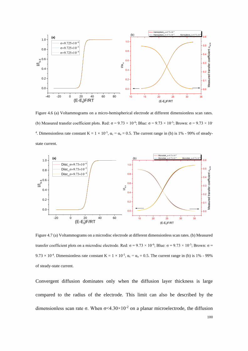
100
Figure 4.6 (a) Voltammograms on a micro-hemispherical electrode at different dimensionless scan rates.
(b) Measured transfer coefficient plots. Red: σ = 9.73 × 10⁻⁶; Blue: σ = 9.73 × 10⁻⁵; Brown: σ = 9.73 × 10-
4. Dimensionless rate constant K = 1 × 10⁻⁵, αc = αa = 0.5. The current range in (b) is 1% - 99% of steady-
state current.
Figure 4.7 (a) Voltammograms on a microdisc electrode at different dimensionless scan rates. (b) Measured
transfer coefficient plots on a microdisc electrode. Red: σ = 9.73 × 10⁻⁶; Blue: σ = 9.73 × 10⁻⁵; Brown: σ =
9.73 × 10⁻⁴. Dimensionless rate constant K = 1 × 10⁻⁵, αc = αa = 0.5. The current range in (b) is 1% - 99%
of steady-state current.
Convergent diffusion dominates only when the diffusion layer thickness is large
compared to the radius of the electrode. This limit can also be described by the
dimensionless scan rate σ. When σ<4.30×10⁻² on a planar microelectrode, the diffusion
-40 -20 0 20 40 60 80
0.0
0.2
0.4
0.6
0.8
1.0I/I s
.s
(E-Ef)F/RT
=−
=−
=−
(a)
-20 0 20 40 60
0.0
0.2
0.4
0.6
0.8
1.0
I/I s
.s
(E-Ef)F/RT
Disc_=−
Disc_=−
Disc_=−
(a)
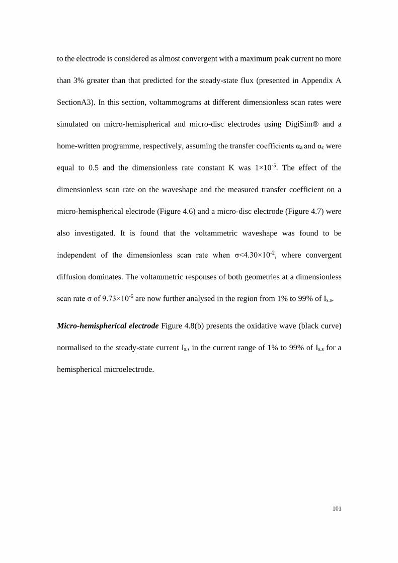
101
to the electrode is considered as almost convergent with a maximum peak current no more
than 3% greater than that predicted for the steady-state flux (presented in Appendix A
SectionA3). In this section, voltammograms at different dimensionless scan rates were
simulated on micro-hemispherical and micro-disc electrodes using DigiSim® and a
home-written programme, respectively, assuming the transfer coefficients αa and αc were
equal to 0.5 and the dimensionless rate constant K was 1×10⁻⁵. The effect of the
dimensionless scan rate on the waveshape and the measured transfer coefficient on a
micro-hemispherical electrode (Figure 4.6) and a micro-disc electrode (Figure 4.7) were
also investigated. It is found that the voltammetric waveshape was found to be
independent of the dimensionless scan rate when σ<4.30×10⁻², where convergent
diffusion dominates. The voltammetric responses of both geometries at a dimensionless
scan rate σ of 9.73×10⁻⁶ are now further analysed in the region from 1% to 99% of Is.s.
Micro-hemispherical electrode Figure 4.8(b) presents the oxidative wave (black curve)
normalised to the steady-state current Is.s in the current range of 1% to 99% of Is.s for a
hemispherical microelectrode.
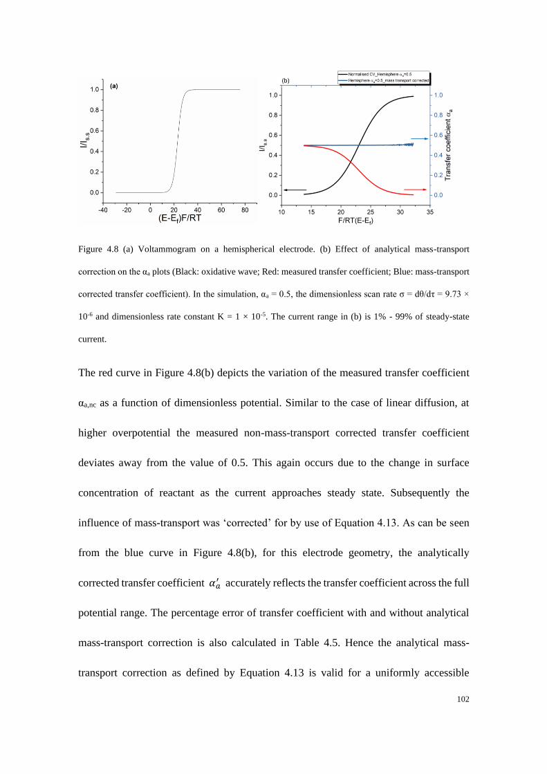
102
Figure 4.8 (a) Voltammogram on a hemispherical electrode. (b) Effect of analytical mass-transport
correction on the αa plots (Black: oxidative wave; Red: measured transfer coefficient; Blue: mass-transport
corrected transfer coefficient). In the simulation, αa = 0.5, the dimensionless scan rate σ = dθ/dτ = 9.73 ×
10-6 and dimensionless rate constant K = 1 × 10⁻⁵. The current range in (b) is 1% - 99% of steady-state
current.
The red curve in Figure 4.8(b) depicts the variation of the measured transfer coefficient
αa,nc as a function of dimensionless potential. Similar to the case of linear diffusion, at
higher overpotential the measured non-mass-transport corrected transfer coefficient
deviates away from the value of 0.5. This again occurs due to the change in surface
concentration of reactant as the current approaches steady state. Subsequently the
influence of mass-transport was ‘corrected’ for by use of Equation 4.13. As can be seen
from the blue curve in Figure 4.8(b), for this electrode geometry, the analytically
corrected transfer coefficient 𝛼𝑎′ accurately reflects the transfer coefficient across the full
potential range. The percentage error of transfer coefficient with and without analytical
mass-transport correction is also calculated in Table 4.5. Hence the analytical mass-
transport correction as defined by Equation 4.13 is valid for a uniformly accessible
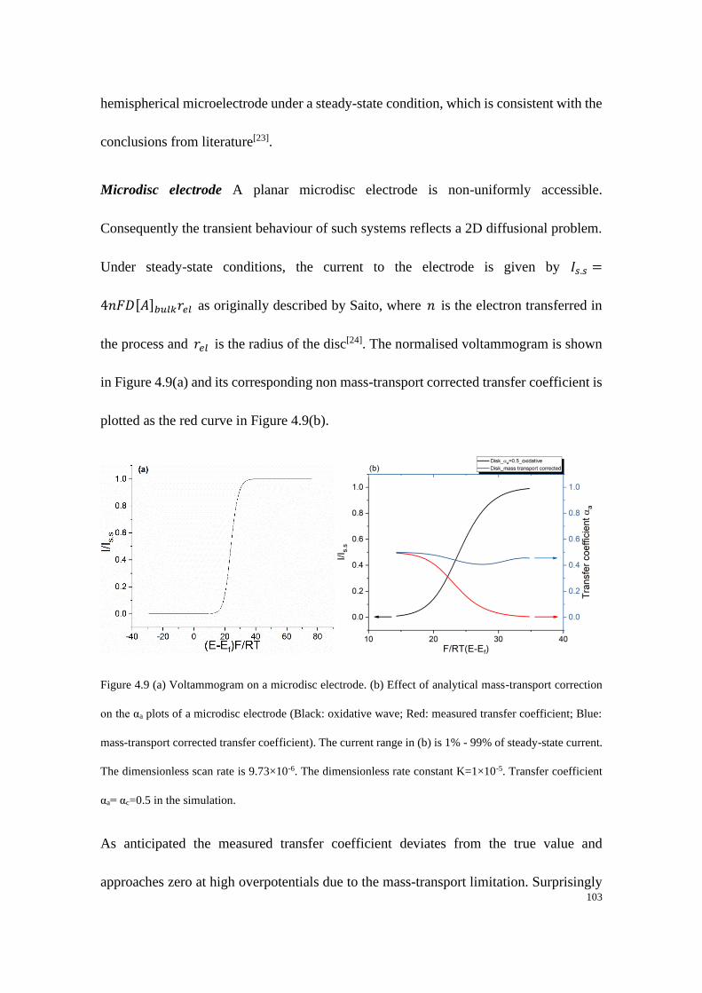
103
hemispherical microelectrode under a steady-state condition, which is consistent with the
conclusions from literature[23].
Microdisc electrode A planar microdisc electrode is non-uniformly accessible.
Consequently the transient behaviour of such systems reflects a 2D diffusional problem.
Under steady-state conditions, the current to the electrode is given by 𝐼𝑠.𝑠 =
4𝑛𝐹𝐷[𝐴]𝑏𝑢𝑙𝑘𝑟𝑒𝑙 as originally described by Saito, where 𝑛 is the electron transferred in
the process and 𝑟𝑒𝑙 is the radius of the disc[24]. The normalised voltammogram is shown
in Figure 4.9(a) and its corresponding non mass-transport corrected transfer coefficient is
plotted as the red curve in Figure 4.9(b).
Figure 4.9 (a) Voltammogram on a microdisc electrode. (b) Effect of analytical mass-transport correction
on the αa plots of a microdisc electrode (Black: oxidative wave; Red: measured transfer coefficient; Blue:
mass-transport corrected transfer coefficient). The current range in (b) is 1% - 99% of steady-state current.
The dimensionless scan rate is 9.73×10⁻⁶. The dimensionless rate constant K=1×10⁻⁵. Transfer coefficient
αa= αc=0.5 in the simulation.
As anticipated the measured transfer coefficient deviates from the true value and
approaches zero at high overpotentials due to the mass-transport limitation. Surprisingly
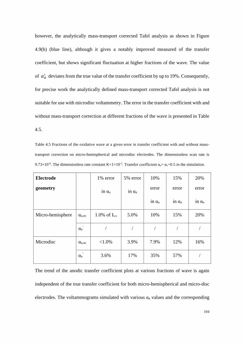
104
however, the analytically mass-transport corrected Tafel analysis as shown in Figure
4.9(b) (blue line), although it gives a notably improved measured of the transfer
coefficient, but shows significant fluctuation at higher fractions of the wave. The value
of 𝛼𝑎′ deviates from the true value of the transfer coefficient by up to 19%. Consequently,
for precise work the analytically defined mass-transport corrected Tafel analysis is not
suitable for use with microdisc voltammetry. The error in the transfer coefficient with and
without mass-transport correction at different fractions of the wave is presented in Table
4.5.
Table 4.5 Fractions of the oxidative wave at a given error in transfer coefficient with and without mass-
transport correction on micro-hemispherical and microdisc electrodes. The dimensionless scan rate is
9.73×10⁻⁶. The dimensionless rate constant K=1×10⁻⁵. Transfer coefficient αa= αc=0.5 in the simulation.
Electrode
geometry
1% error
in αa
5% error
in αa
10%
error
in αa
15%
error
in αa
20%
error
in αa
Micro-hemisphere αa,nc 1.0% of Is.s 5.0% 10% 15% 20%
αa’ / / / / /
Microdisc αa,nc <1.0% 3.9% 7.9% 12% 16%
αa’ 3.6% 17% 35% 57% /
The trend of the anodic transfer coefficient plots at various fractions of wave is again
independent of the true transfer coefficient for both micro-hemispherical and micro-disc
electrodes. The voltammograms simulated with various αa values and the corresponding
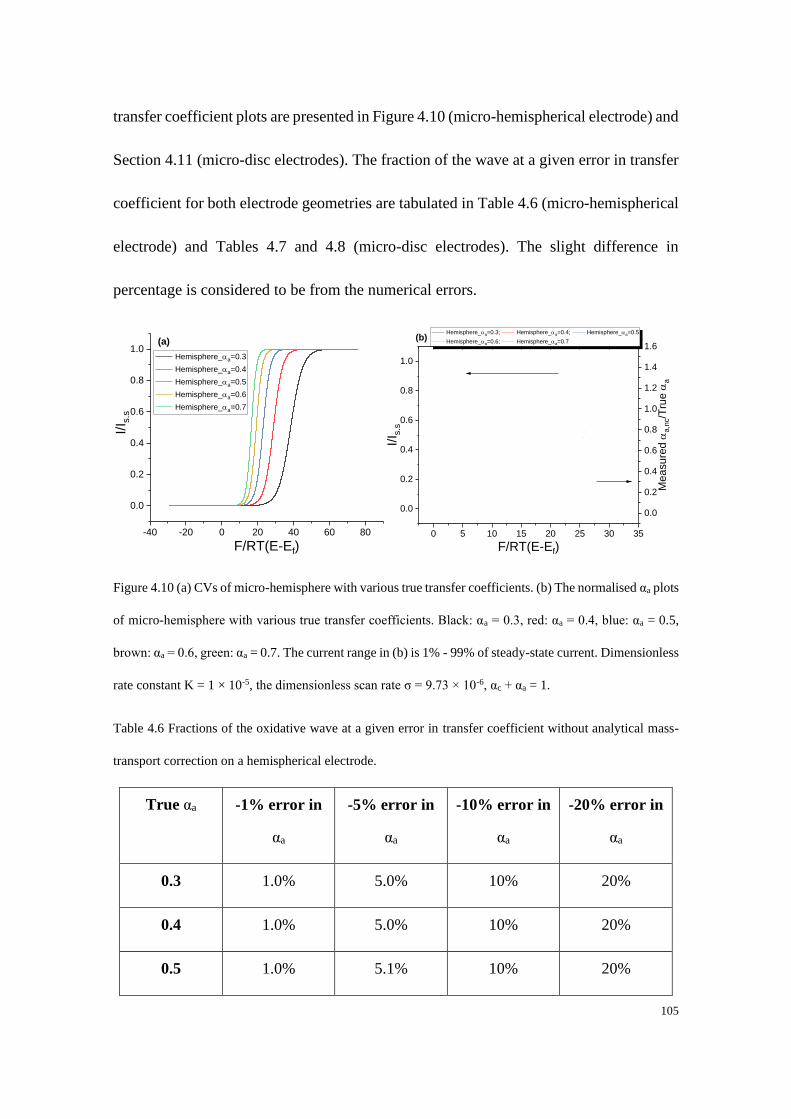
105
transfer coefficient plots are presented in Figure 4.10 (micro-hemispherical electrode) and
Section 4.11 (micro-disc electrodes). The fraction of the wave at a given error in transfer
coefficient for both electrode geometries are tabulated in Table 4.6 (micro-hemispherical
electrode) and Tables 4.7 and 4.8 (micro-disc electrodes). The slight difference in
percentage is considered to be from the numerical errors.
Figure 4.10 (a) CVs of micro-hemisphere with various true transfer coefficients. (b) The normalised αa plots
of micro-hemisphere with various true transfer coefficients. Black: αa = 0.3, red: αa = 0.4, blue: αa = 0.5,
brown: αa = 0.6, green: αa = 0.7. The current range in (b) is 1% - 99% of steady-state current. Dimensionless
rate constant K = 1 × 10⁻⁵, the dimensionless scan rate σ = 9.73 × 10⁻⁶, αc + αa = 1.
Table 4.6 Fractions of the oxidative wave at a given error in transfer coefficient without analytical mass-
transport correction on a hemispherical electrode.
True αa -1% error in
αa
-5% error in
αa
-10% error in
αa
-20% error in
αa
0.3 1.0% 5.0% 10% 20%
0.4 1.0% 5.0% 10% 20%
0.5 1.0% 5.1% 10% 20%
-40 -20 0 20 40 60 80
0.0
0.2
0.4
0.6
0.8
1.0
I/I s
.s
F/RT(E-Ef)
Hemisphere_a=0.3
Hemisphere_a=0.4
Hemisphere_a=0.5
Hemisphere_a=0.6
Hemisphere_a=0.7
(a)
0 5 10 15 20 25 30 35
0.0
0.2
0.4
0.6
0.8
1.0
Hemisphere_a=0.3; Hemisphere_a=0.4; Hemisphere_a=0.5
Hemisphere_a=0.6; Hemisphere_a=0.7
F/RT(E-Ef)
I/I s
.s
(b)
0.0
0.2
0.4
0.6
0.8
1.0
1.2
1.4
1.6
Mea
su
red
a,n
c/T
rue
a
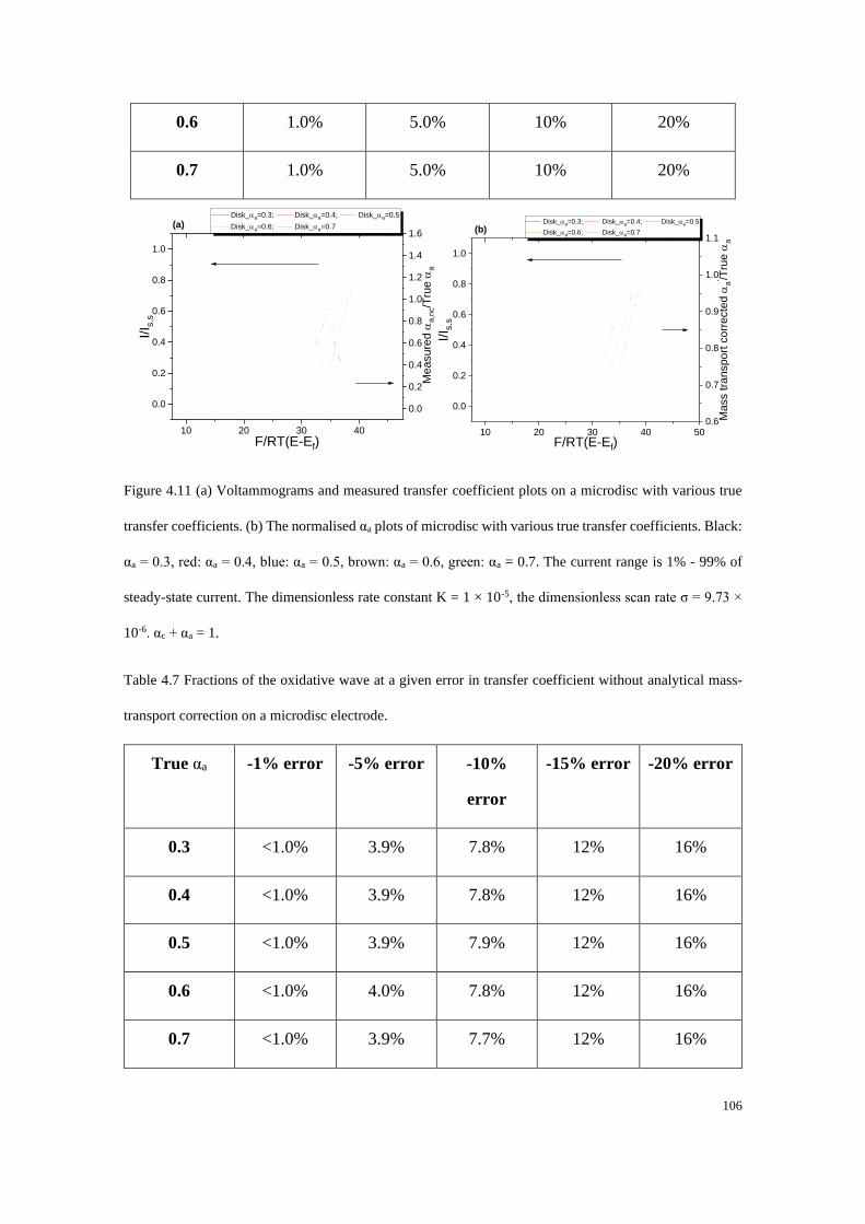
106
0.6 1.0% 5.0% 10% 20%
0.7 1.0% 5.0% 10% 20%
Figure 4.11 (a) Voltammograms and measured transfer coefficient plots on a microdisc with various true
transfer coefficients. (b) The normalised αa plots of microdisc with various true transfer coefficients. Black:
αa = 0.3, red: αa = 0.4, blue: αa = 0.5, brown: αa = 0.6, green: αa = 0.7. The current range is 1% - 99% of
steady-state current. The dimensionless rate constant K = 1 × 10⁻⁵, the dimensionless scan rate σ = 9.73 ×
10-6. αc + αa = 1.
Table 4.7 Fractions of the oxidative wave at a given error in transfer coefficient without analytical mass-
transport correction on a microdisc electrode.
True αa -1% error -5% error -10%
error
-15% error -20% error
0.3 <1.0% 3.9% 7.8% 12% 16%
0.4 <1.0% 3.9% 7.8% 12% 16%
0.5 <1.0% 3.9% 7.9% 12% 16%
0.6 <1.0% 4.0% 7.8% 12% 16%
0.7 <1.0% 3.9% 7.7% 12% 16%
10 20 30 40
0.0
0.2
0.4
0.6
0.8
1.0
Disk_a=0.3; Disk_a=0.4; Disk_a=0.5
Disk_a=0.6; Disk_a=0.7
F/RT(E-Ef)
I/I s
.s
(a)
0.0
0.2
0.4
0.6
0.8
1.0
1.2
1.4
1.6
Measure
d
a,n
c/T
rue
a10 20 30 40 50
0.0
0.2
0.4
0.6
0.8
1.0
Disk_a=0.3; Disk_a=0.4; Disk_a=0.5
Disk_a=0.6; Disk_a=0.7
F/RT(E-Ef)I/I s
.s
(b)
0.6
0.7
0.8
0.9
1.0
1.1
Mass tra
nspo
rt c
orr
ecte
d
a' /T
rue
a
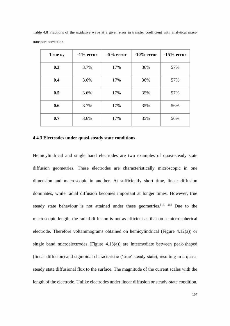
107
Table 4.8 Fractions of the oxidative wave at a given error in transfer coefficient with analytical mass-
transport correction.
True αa -1% error -5% error -10% error -15% error
0.3 3.7% 17% 36% 57%
0.4 3.6% 17% 36% 57%
0.5 3.6% 17% 35% 57%
0.6 3.7% 17% 35% 56%
0.7 3.6% 17% 35% 56%
4.4.3 Electrodes under quasi-steady state conditions
Hemicylindrical and single band electrodes are two examples of quasi-steady state
diffusion geometries. These electrodes are characteristically microscopic in one
dimension and macroscopic in another. At sufficiently short time, linear diffusion
dominates, while radial diffusion becomes important at longer times. However, true
steady state behaviour is not attained under these geometries.[19, 25] Due to the
macroscopic length, the radial diffusion is not as efficient as that on a micro-spherical
electrode. Therefore voltammograms obtained on hemicylindrical (Figure 4.12(a)) or
single band microelectrodes (Figure 4.13(a)) are intermediate between peak-shaped
(linear diffusion) and sigmoidal characteristic (‘true’ steady state), resulting in a quasi-
steady state diffusional flux to the surface. The magnitude of the current scales with the
length of the electrode. Unlike electrodes under linear diffusion or steady-state condition,
108
the voltammetric waveshape on micro-hemicylinder and single microband is sensitive to
the dimensionless scan rate. As can be seen from the Figure 4.12 (a) (micro-
hemicylindrical electrode) and Figure 4.13 (a) (single microband), the voltammogram
becomes more peak-shaped at higher dimensionless scan rates as a result of larger
contribution from linear diffusion and more sigmoidal-like at sufficiently small
dimensionless scan rates due to enhanced mass transport from non-linear diffusion. It is
also found that this improvement in the estimation of transfer coefficient using analytical
mass-transport correction becomes smaller at higher dimensionless scan rates where the
linear diffusion contribution is larger, which further proves the assumption of the
analytical mass-transport correction, as shown in Table 4.9 (micro-hemicylindrical
electrode) and Table 4.10 (single microband electrode).
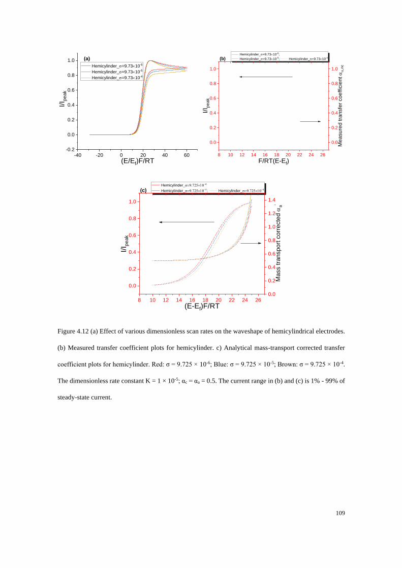
109
Figure 4.12 (a) Effect of various dimensionless scan rates on the waveshape of hemicylindrical electrodes.
(b) Measured transfer coefficient plots for hemicylinder. c) Analytical mass-transport corrected transfer
coefficient plots for hemicylinder. Red: σ = 9.725 × 10⁻⁶; Blue: σ = 9.725 × 10⁻⁵; Brown: σ = 9.725 × 10⁻⁴.
The dimensionless rate constant K = 1 × 10⁻⁵; αc = αa = 0.5. The current range in (b) and (c) is 1% - 99% of
steady-state current.
-40 -20 0 20 40 60-0.2
0.0
0.2
0.4
0.6
0.8
1.0I/I p
ea
k
(E/Ef)F/RT
Hemicylinder_=9.7310-6
Hemicylinder_=9.7310-5
Hemicylinder_=9.7310-4
(a)
8 10 12 14 16 18 20 22 24 26
0.0
0.2
0.4
0.6
0.8
1.0
Hemicylinder_=9.7310-6;
Hemicylinder_=9.7310-5; Hemicylinder_=9.7310-4
F/RT(E-Ef)
I/I p
ea
k
(b)
0.0
0.2
0.4
0.6
0.8
1.0
Me
asu
red
tra
nsfe
r co
effic
ien
t n
c
8 10 12 14 16 18 20 22 24 26
0.0
0.2
0.4
0.6
0.8
1.0
Hemicylinder_=−
Hemicylinder_=−; Hemicylinder_=−
(E-Ef)F/RT
I/I p
ea
k
(c)
0.0
0.2
0.4
0.6
0.8
1.0
1.2
1.4
Mass tra
nspo
rt c
orr
ecte
d
a'
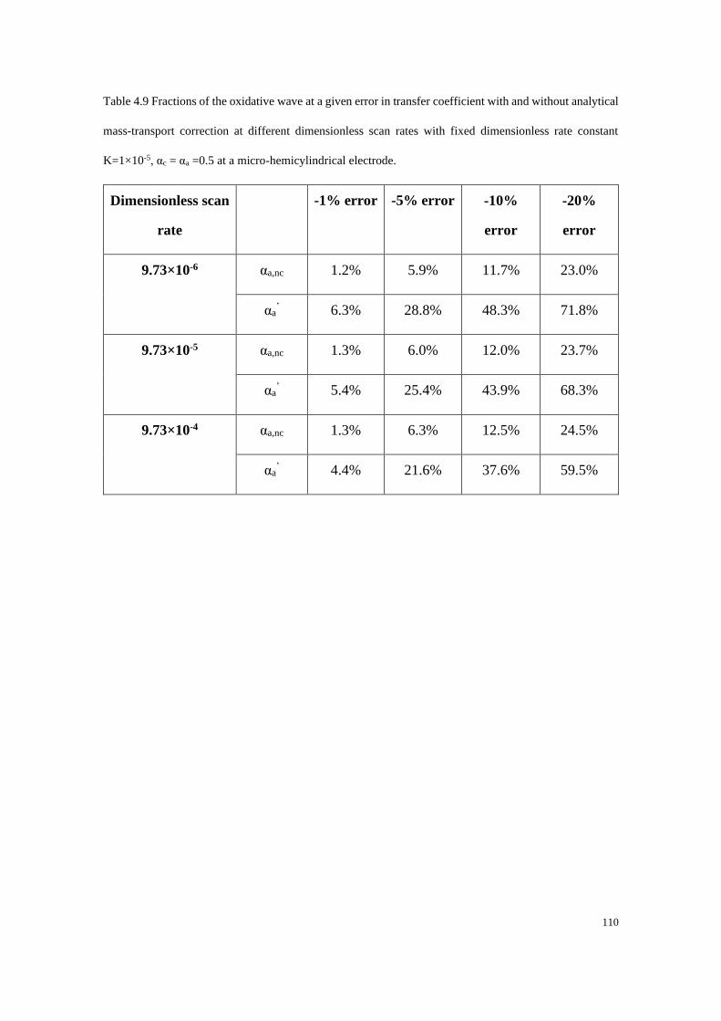
110
Table 4.9 Fractions of the oxidative wave at a given error in transfer coefficient with and without analytical
mass-transport correction at different dimensionless scan rates with fixed dimensionless rate constant
K=1×10⁻⁵, αc = αa =0.5 at a micro-hemicylindrical electrode.
Dimensionless scan
rate
-1% error -5% error -10%
error
-20%
error
9.73×10⁻⁶ αa,nc 1.2% 5.9% 11.7% 23.0%
αa’ 6.3% 28.8% 48.3% 71.8%
9.73×10⁻⁵ αa,nc 1.3% 6.0% 12.0% 23.7%
αa’ 5.4% 25.4% 43.9% 68.3%
9.73×10⁻⁴ αa,nc 1.3% 6.3% 12.5% 24.5%
αa’ 4.4% 21.6% 37.6% 59.5%
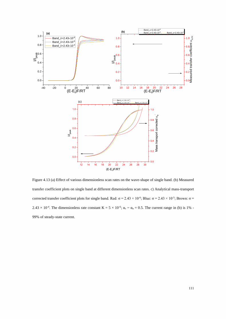
111
Figure 4.13 (a) Effect of various dimensionless scan rates on the wave-shape of single band. (b) Measured
transfer coefficient plots on single band at different dimensionless scan rates. c) Analytical mass-transport
corrected transfer coefficient plots for single band. Red: σ = 2.43 × 10⁻⁶; Blue: σ = 2.43 × 10⁻⁵; Brown: σ =
2.43 × 10⁻⁴. The dimensionless rate constant K = 5 × 10⁻⁶; αc = αa = 0.5. The current range in (b) is 1% -
99% of steady-state current.
-40 -20 0 20 40 60 80
0.0
0.2
0.4
0.6
0.8
1.0I/I p
ea
k
(E-Ef)F/RT
Band_=2.4310-6
Band_=2.4310-5
Band_=2.4310-4
(a)
10 12 14 16 18 20 22 24 26 28
0.0
0.2
0.4
0.6
0.8
1.0
Band_=2.4310-6
Band_=2.4310-5; Band_=2.4310-4
(E-Ef)F/RT
I/I p
ea
k
(b)
0.0
0.2
0.4
0.6
0.8
1.0
Mea
su
red tra
nsfe
r coe
ffic
ien
t
a,n
c
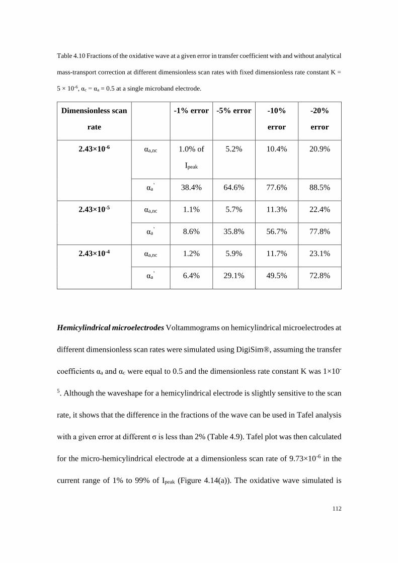
112
Table 4.10 Fractions of the oxidative wave at a given error in transfer coefficient with and without analytical
mass-transport correction at different dimensionless scan rates with fixed dimensionless rate constant K =
5 × 10⁻⁶, αc = αa = 0.5 at a single microband electrode.
Dimensionless scan
rate
-1% error -5% error -10%
error
-20%
error
2.43×10⁻⁶ αa,nc 1.0% of
Ipeak
5.2% 10.4% 20.9%
αa’ 38.4% 64.6% 77.6% 88.5%
2.43×10⁻⁵ αa,nc 1.1% 5.7% 11.3% 22.4%
αa’ 8.6% 35.8% 56.7% 77.8%
2.43×10⁻⁴ αa,nc 1.2% 5.9% 11.7% 23.1%
αa’ 6.4% 29.1% 49.5% 72.8%
Hemicylindrical microelectrodes Voltammograms on hemicylindrical microelectrodes at
different dimensionless scan rates were simulated using DigiSim®, assuming the transfer
coefficients αa and αc were equal to 0.5 and the dimensionless rate constant K was 1×10-
5. Although the waveshape for a hemicylindrical electrode is slightly sensitive to the scan
rate, it shows that the difference in the fractions of the wave can be used in Tafel analysis
with a given error at different σ is less than 2% (Table 4.9). Tafel plot was then calculated
for the micro-hemicylindrical electrode at a dimensionless scan rate of 9.73×10⁻⁶ in the
current range of 1% to 99% of Ipeak (Figure 4.14(a)). The oxidative wave simulated is
113
normalised relative to its peak current as shown as the black curve in Figure 4.14(b). The
measured non mass-transport corrected transfer coefficient 𝛼𝑎,𝑛𝑐 (red curve) again
deviates from its true value at higher potentials, as is seen under other geometries. The
removal of mass-transport effect was attempted using the analytical approximation to get
a better correction for the measure of the transfer coefficient as shown as the blue curve
in Figure 4.14(b).
Figure 4.14 (a) Voltammogram on a micro-hemicylindrical electrode. (b) Effect of analytical mass-
transport correction on the transfer coefficient plots of hemicylinder (Black: oxidative wave; Red: measured
transfer coefficient; Blue: mass-transport corrected transfer coefficient). The current range in (b) is 1% -
99% of steady-state current. The dimensionless scan rate is 9.73×10⁻⁶. The dimensionless rate constant
K=1×10⁻⁵. Transfer coefficients αa= αc=0.5 in the simulation.
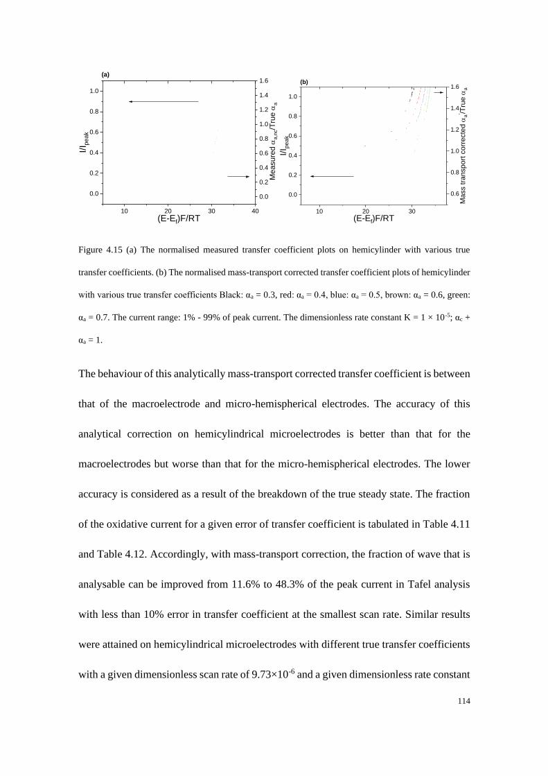
114
Figure 4.15 (a) The normalised measured transfer coefficient plots on hemicylinder with various true
transfer coefficients. (b) The normalised mass-transport corrected transfer coefficient plots of hemicylinder
with various true transfer coefficients Black: αa = 0.3, red: αa = 0.4, blue: αa = 0.5, brown: αa = 0.6, green:
αa = 0.7. The current range: 1% - 99% of peak current. The dimensionless rate constant K = 1 × 10⁻⁵; αc +
αa = 1.
The behaviour of this analytically mass-transport corrected transfer coefficient is between
that of the macroelectrode and micro-hemispherical electrodes. The accuracy of this
analytical correction on hemicylindrical microelectrodes is better than that for the
macroelectrodes but worse than that for the micro-hemispherical electrodes. The lower
accuracy is considered as a result of the breakdown of the true steady state. The fraction
of the oxidative current for a given error of transfer coefficient is tabulated in Table 4.11
and Table 4.12. Accordingly, with mass-transport correction, the fraction of wave that is
analysable can be improved from 11.6% to 48.3% of the peak current in Tafel analysis
with less than 10% error in transfer coefficient at the smallest scan rate. Similar results
were attained on hemicylindrical microelectrodes with different true transfer coefficients
with a given dimensionless scan rate of 9.73×10⁻⁶ and a given dimensionless rate constant
10 20 30 40
0.0
0.2
0.4
0.6
0.8
1.0
(E-Ef)F/RT
I/I p
ea
k
(a)
0.0
0.2
0.4
0.6
0.8
1.0
1.2
1.4
1.6
Measure
d
a,n
c/T
rue
a
10 20 30
0.0
0.2
0.4
0.6
0.8
1.0
(E-Ef)F/RT
I/I p
ea
k
(b)
0.6
0.8
1.0
1.2
1.4
1.6
Ma
ss t
ran
sp
ort
co
rre
cte
d
a' /T
rue
a

115
of 1×10⁻⁵. The corresponding transfer coefficient plots with and without analytical mass-
transport correction are presented in Figure 4.15. The fraction of the voltammetric wave
at a given error in transfer coefficient is tabulated in Table 4.11 and 4.12.
Table 4.11 Fractions of the oxidative wave at a given error in transfer coefficient without analytical mass-
transport correction at a micro-hemicylindrical electrode.
True αa -1% error -5% error -10% error -20% error
0.3 1.3% 5.9% 11.5% 22.9%
0.4 1.2% 5.9% 11.7% 22.9%
0.5 1.2% 5.9% 11.6% 23.0%
0.6 1.2% 5.9% 11.7% 22.9%
0.7 1.2% 5.9% 11.6% 23.0%
Table 4.12 Fractions of the oxidative wave at a given error in transfer coefficient with analytical mass-
transport correction at a micro-hemicylindrical electrode.
True αa +1% error +5% error +10% error +20% error
0.3 6.2% 30.8% 49.2% 72.5%
0.4 6.1% 28.9% 49.1% 72.0%
0.5 6.4% 28.4% 48.3% 71.8%
0.6 6.0% 27.7% 48.6% 71.8%
0.7 6.2% 27.6% 47.8% 71.3%
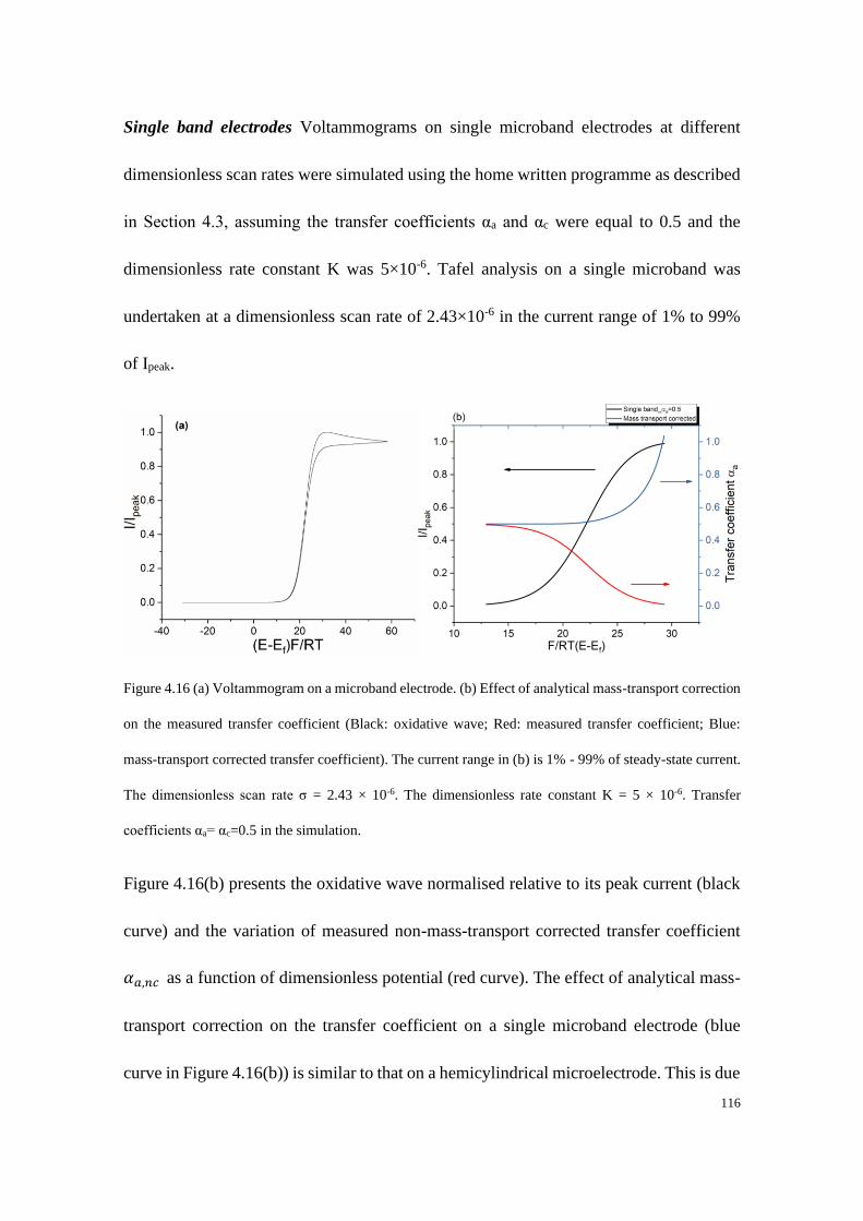
116
Single band electrodes Voltammograms on single microband electrodes at different
dimensionless scan rates were simulated using the home written programme as described
in Section 4.3, assuming the transfer coefficients αa and αc were equal to 0.5 and the
dimensionless rate constant K was 5×10⁻⁶. Tafel analysis on a single microband was
undertaken at a dimensionless scan rate of 2.43×10⁻⁶ in the current range of 1% to 99%
of Ipeak.
Figure 4.16 (a) Voltammogram on a microband electrode. (b) Effect of analytical mass-transport correction
on the measured transfer coefficient (Black: oxidative wave; Red: measured transfer coefficient; Blue:
mass-transport corrected transfer coefficient). The current range in (b) is 1% - 99% of steady-state current.
The dimensionless scan rate σ = 2.43 × 10⁻⁶. The dimensionless rate constant K = 5 × 10⁻⁶. Transfer
coefficients αa= αc=0.5 in the simulation.
Figure 4.16(b) presents the oxidative wave normalised relative to its peak current (black
curve) and the variation of measured non-mass-transport corrected transfer coefficient
𝛼𝑎,𝑛𝑐 as a function of dimensionless potential (red curve). The effect of analytical mass-
transport correction on the transfer coefficient on a single microband electrode (blue
curve in Figure 4.16(b)) is similar to that on a hemicylindrical microelectrode. This is due
117
to both the quasi-steady state condition rather than a true steady state and the non-
uniformly accessibility of the single microband. According to the results of the calculated
fraction of the oxidative wave at given errors in transfer coefficient, with analytical mass-
transport correction, the fraction of the peak current can be improved from 4.9% to 64.5%
in Tafel analysis with less than 5% error in transfer coefficient. Similar to hemicylindrical
electrodes, the analytical correction works better at lower dimensionless scan rates due to
the increased radial diffusion to the electrode.
Voltammograms with other different transfer coefficients (αa=0.3, 0.4, 0.6 and 0.7) with
a given dimensionless scan rate of 2.43×10⁻⁶ and a given dimensionless rate constant of
5×10⁻⁶ were also simulated and analysed via the same method. A similar trend was
observed in the case of the measured non mass-transport corrected transfer coefficient as
shown in Figure 4.17. However, unlike the results for other geometries, the fraction of
the oxidative wave which can be used in Tafel analysis at given errors increases with a
larger transfer coefficient after analytical mass-transport correction. For example, from
the data shown in Table 4.13 and 4.14, up to 82% of the oxidative current can be used in
Tafel analysis with a 10% error in transfer coefficient when αa equals to 0.7.
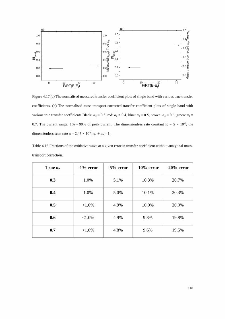
118
Figure 4.17 (a) The normalised measured transfer coefficient plots of single band with various true transfer
coefficients. (b) The normalised mass-transport corrected transfer coefficient plots of single band with
various true transfer coefficients Black: αa = 0.3, red: αa = 0.4, blue: αa = 0.5, brown: αa = 0.6, green: αa =
0.7. The current range: 1% - 99% of peak current. The dimensionless rate constant K = 5 × 10⁻⁶; the
dimensionless scan rate σ = 2.43 × 10⁻⁶; αc + αa = 1.
Table 4.13 Fractions of the oxidative wave at a given error in transfer coefficient without analytical mass-
transport correction.
True αa -1% error -5% error -10% error -20% error
0.3 1.0% 5.1% 10.3% 20.7%
0.4 1.0% 5.0% 10.1% 20.3%
0.5 <1.0% 4.9% 10.0% 20.0%
0.6 <1.0% 4.9% 9.8% 19.8%
0.7 <1.0% 4.8% 9.6% 19.5%
0 10 20 30
0.0
0.2
0.4
0.6
0.8
1.0
F/RT(E-Ef)
I/I p
ea
k
(a)
0.0
0.2
0.4
0.6
0.8
1.0
Me
asu
red
a,n
c/ T
rue
a
0 10 20 30
0.0
0.2
0.4
0.6
0.8
1.0
F/RT(E-Ef)
I/I p
ea
k
(b)
0.6
0.8
1.0
1.2
1.4
1.6
Ma
ss t
ran
sp
ort
co
rre
cte
d
a' /T
rue
a
119
Table 4.14 Fractions of the oxidative wave at a given error in transfer coefficient with analytical mass-
transport correction.
True αa +1% error +5% error +10% error +20% error
0.3 22.4% 55.4% 72.0% 85.9%
0.4 30.1% 60.1% 74.9% 87.3%
0.5 38.4% 64.5% 77.6% 88.5%
0.6 46.2% 68.5% 79.9% 89.6%
0.7 53.2% 72.0% 82.0% 90.6%
4.5 Conclusions
For all electrode geometries, and in the absence of mass-transport correction to the
resulting flux, the measured non mass-transport corrected transfer coefficient deviates
significantly from its true value even when only currents less than 10% of the steady-state
or peak current are analysed in Tafel analysis. The exact fraction of the voltammetric
wave that can be used in Tafel analysis is sensitive to the electrode geometry and the
prevailing mass-transport regime. Due to the variation of 𝛼𝑎,𝑛𝑐 as a function of potential
as a result of the influence of mass transport, care must be taken in analysing such data
so as to not wrongly conclude that curvature in such Tafel plots reflects a sensitivity of
the underlying transfer coefficient to the electrode potential.
The use of a plot of 𝑙𝑛 |1
𝐼−
1
𝐼𝑙𝑖𝑚| against θ to provide a mass-transport corrected Tafel
plot is strictly only applicable to cases where the electrode is uniformly accessible and is

120
under a true steady-state diffusion regime. The use of such a mass-transport corrected
Tafel plot even for micro-disc electrodes is found to potentially result in significant errors
in the measured transfer coefficient (up to 19%). For the quasi-steady-state regimes with
specific dimensionless constants, the fraction of the voltammetric wave can be improved
to 48.3% (micro-hemicylinder) and 77.6% (single microband) with less than 10% error
in transfer coefficient after this analytical correction. Moreover, such an analytical mass-
transport correction completely fails when applied to voltammetry measured under a
linear diffusion regime (macroelectrode). The new empirical mass-transport correction
presented allows an improved estimation of the transfer coefficient for macroelectrode
geometry.
References:
[1] D. Li, C. Lin, C. Batchelor-McAuley, L. Chen, R. G. Compton, Journal of Electroanalytical
Chemistry 2018, 826, 117-124.
[2] aF. Scholz, Electroanalytical Methods: Guide to Experiments and Applications, Springer Berlin
Heidelberg, 2009; bM. C. Henstridge, R. G. Compton, Journal of Electroanalytical Chemistry
2012, 681, 109-112.
[3] aR. Guidelli, R. G. Compton, J. M. Feliu, E. Gileadi, J. Lipkowski, W. Schmickler, S. Trasatti,
Pure and Applied Chemistry 2014, 86, 245-258; bR. Guidelli, R. G. Compton, J. M. Feliu, E.
Gileadi, J. Lipkowski, W. Schmickler, S. Trasatti, Pure and Applied Chemistry 2014, 86, 259-262.
[4] S. Fletcher, Journal of Solid State Electrochemistry 2008, 13, 537-549.
[5] aW. Sheng, H. A. Gasteiger, Y. Shao-Horn, Journal of The Electrochemical Society 2010, 157,
B1529; bD. V. Esposito, S. T. Hunt, A. L. Stottlemyer, K. D. Dobson, B. E. McCandless, R. W.
Birkmire, J. G. Chen, Angew Chem Int Ed Engl 2010, 49, 9859-9862.
[6] R. G. A. B. Compton, Craig E, Understanding Voltammetry, third ed., World Scientific, 2018.
[7] C. Batchelor-McAuley, R. G. Compton, Journal of Electroanalytical Chemistry 2012, 669, 73-81.
[8] aR. A. Marcus, The Journal of Chemical Physics 1965, 43, 679-701; bR. A. Marcus, N. Sutin,
Biochimica et Biophysica Acta (BBA) - Reviews on Bioenergetics 1985, 811, 265-322; cN. S. Hush,
The Journal of Chemical Physics 1958, 28, 962-972.
121
[9] E. Laborda, M. C. Henstridge, C. Batchelor-McAuley, R. G. Compton, Chemical Society Reviews
2013, 42, 4894-4905.
[10] V. Mirceski, E. Laborda, D. Guziejewski, R. G. Compton, Analytical Chemistry 2013, 85, 5586-
5594.
[11] aM. C. Henstridge, E. Laborda, Y. Wang, D. Suwatchara, N. Rees, Á. Molina, F. Martínez-Ortiz,
R. G. Compton, Journal of Electroanalytical Chemistry 2012, 672, 45-52; bE. Laborda, M. C.
Henstridge, R. G. Compton, Journal of Electroanalytical Chemistry 2012, 681, 96-102.
[12] aJ. M. Savéant, D. Tessier, Journal of Electroanalytical Chemistry and Interfacial
Electrochemistry 1975, 65, 57-66; bC. E. D. Chidsey, Science 1991, 251, 919-922.
[13] aT. Erdey-Grúz, M. Volmer, 1930, 150A, 203; bJ. Butler, Transactions of the Faraday Society
1924, 19, 729-733.
[14] aO. V. Klymenko, R. G. Compton, Journal of Electroanalytical Chemistry 2004, 571, 207-210;
bN. V. Rees, J. A. Alden, R. A. W. Dryfe, B. A. Coles, R. G. Compton, The Journal of Physical
Chemistry 1995, 99, 14813-14818.
[15] A. D. McNaught, A. Wilkinson, Compendium of chemical terminology, Vol. 1669, Blackwell
Science Oxford, 1997.
[16] W. J. Albery, Philosophical Transactions of the Royal Society of London. Series A, Mathematical
and Physical Sciences 1981, 302, 221-235.
[17] aM. Rudolph, Journal of electroanalytical chemistry and interfacial electrochemistry 1991, 314,
13-22; bM. Rudolph, Journal of Electroanalytical Chemistry 1992, 338, 85-98; cM. Rudolph,
Journal of Electroanalytical Chemistry 1994, 375, 89-99.
[18] O. V. Klymenko, R. G. Evans, C. Hardacre, I. B. Svir, R. G. Compton, Journal of
Electroanalytical Chemistry 2004, 571, 211-221.
[19] C. Amatore, B. Fosset, Analytical Chemistry 1996, 68, 4377-4388.
[20] R. G. Compton, E. A Laborda, K. R. A Ward, Understanding Voltammetry: Simulation of
Eelctrode Processes, Imperial College Press, 2013.
[21] C. Batchelor-McAuley, M. Yang, E. M. Hall, R. G. Compton, Journal of Electroanalytical
Chemistry 2015, 758, 1-6.
[22] N. Eliaz, E. Gileadi, Physical Electrochemistry: Fundamentals, Techniques, and Applications,
Wiley, 2019.
[23] I. Streeter, R. G. Compton, Electrochimica acta 2007, 52, 4305-4311.
[24] Y. Saito, Review of Polarography 1968, 15, 177-187.
[25] aJ. D. Seibold, E. R. Scott, H. S. White, Journal of Electroanalytical Chemistry and Interfacial
Electrochemistry 1989, 264, 281-289; bC. A. Amatore, B. Fosset, M. R. Deakin, R. M. Wightman,
Journal of Electroanalytical Chemistry and Interfacial Electrochemistry 1987, 225, 33-48.
122
Chapter 5
Some Thoughts about Reporting the Electrocatalytic
Performance of Nanomaterials
Chapter 4 explored the use of Tafel analysis which is widely used for evaluating electro-
catalysts. In this chapter, we further develop, more generally, some thoughts on reporting
electrocatalytic activity of electrocatalysts, at least, from an electrochemical perspective,
which are (surprisingly) often presented incorrectly in the ever expanding literature on
electrocatalysts. In particular, we have been stimulated to consider the topic of this work
by an Editorial[1] in ACS Nano which recently provided ‘guidance’ on the ‘best practices’
for the measuring and reporting the activity of new electrocatalytic materials. In the
following we do not seek to provide an alternative set of ‘best practice guidelines’ nor a
‘set of materials characterisation requisites’ – this is likely ultimately an appropriate
activity for an IUPAC committee – but rather correct, amplify and develop the discussion
provided by the Editors of ACS Nano highlighting areas where we believe additional
input is desirable and helpful. We focus on six topics that relate to recommendations made
in the Editorial. In each section we start by making a brief statement that we believe is
correct but different to that made by D. Voiry et al [1]. This statement is then followed by
a more in-depth discussion and exploration of the issue at hand.

123
This work presented in this chapter has been published as a first author paper in Applied
Materials Today[2] and was carried out in collaboration with Dr. Christopher Batchelor-
McAuley.
5.1 Standard, formal and equilibrium potentials
The standard redox potential is not under most conditions equivalent to the equilibrium
potential. The standard potential is the equilibrium electrode potential defined at
standard conditions (STP) with all the electroactive species at unit activity and gases at
standard pressure (assuming ideal behaviour of the gas).
The following definitions are vital to aspects discussed later. To maintain a level of clarity
we focus on the example of a simple one electron transfer process as given by:
A(aq) + e- = B(aq) (5.1)
For this reaction the Nernst equation for the electrode potential (E) is:
𝐸 = 𝐸𝐴/𝐵⦵ −
𝑅𝑇
𝐹𝑙𝑛
𝑎𝐵
𝑎𝐴 (5.2)
where 𝑎i is the activity for the ith species and 𝐸𝐴/𝐵⦵
is the standard redox potential of the
A/B redox couple. This latter value is directly related to the standard Gibbs energy of the
reaction. If we express the solution phase activities of these electroactive solutes in terms
of their activity coefficients on a concentration basis then using the expression 𝑎𝑖 =
𝛾𝑖𝑐𝑖/𝑐⦵, where 𝑐⦵ is the standard concentration (1 mol dm-3) we can write:

124
𝐸 = 𝐸𝐴/𝐵⦵ −
𝑅𝑇
𝐹𝑙𝑛
𝛾𝐵
𝛾𝐴−
𝑅𝑇
𝐹𝑙𝑛
𝑐𝐵
𝑐𝐴 (5.3)
where 𝛾𝑖 is the activity coefficient and noting that the standard concentration terms have
cancelled out, in cases where the stoichiometry of the reaction is not unity this is not the
case. The formal (aka conditional) potential (𝐸𝑓,𝐴/𝐵⦵ ) of the A/B couple is then:
𝐸𝑓,𝐴/𝐵⦵ = 𝐸𝐴/𝐵
⦵ −𝑅𝑇
𝐹𝑙𝑛
𝛾𝐵
𝛾𝐴 (5.4)
First, the formal potential is not a fixed value solely dependent on the A/B couple but is
specific to a given set of experimental conditions. If the activity coefficients of the
electroactive species change, the formal potential is correspondingly altered. For this one-
electron case only if 𝛾𝐵
𝛾𝐴= 1 does the standard potential equal the formal potential.
Second, in contrast to the above case where both the reactant and product are solutes, if
the reaction involves a gas then the standard and formal potentials often differ markedly.[3]
This arises due to the fact that most non-polar gases (such as hydrogen or oxygen) have
a low solubility in aqueous solution.[4] Hence, at one bar pressure the gas is commonly
only present in solution at millimolar concentrations; in contrast, the formal potential is
defined at (a possibly hypothetical)[5] unit concentration. As such the solution phase
dissolved gas concentration is often three orders of magnitude different between these
two definitions.
For a simple one-electron transfer process we can define the equilibrium potential as:[6]
𝐸𝑒𝑞,𝐴/𝐵 = 𝐸𝑓,𝐴/𝐵⦵ −
𝑅𝑇
𝐹𝑙𝑛
𝑐𝐵
𝑐𝐴 (5.5)
125
Even for this simple one electron transfer reaction, Equation 5.5 is explicitly sensitive to
the ratio of the oxidized (A) and reduced (B) species. If a solution contains one order of
magnitude higher concentration of the product as compared to the reactant the equilibrium
potential will be ~59.1 mV negative of the formal potential of the system. This may seem
a moot point but the differences between these definitions become even more pronounced
if an electrode reaction involves multiple steps. For example if the reaction involves the
transfer of one proton per electron then the equilibrium potential varies with 59.1 mV per
pH. Electrocatalytic experiments performed at near neutral pH are often far from being
under standard conditions!
5.2 How should we quantify electrode-kinetics?
For a half-cell reaction the idea of the exchange current (i0) is only directly relevant in
practical situations where both the electroactive product and reactant are present in the
bulk solution phase and the reaction is to some extent reversible. Consequently, we cannot
use i0 as parameter for generally defining electrocatalytic activity.
In electrochemistry there are two common formulations of the Butler-Volmer equation.
First the more general form used by physical electrochemists which is close to that first
derived by Erdey-Gruz and Volmer:[7]
𝐼 = −𝐹𝐴𝑘𝐴/𝐵0 (c𝐴,0exp (
−𝛼𝑐𝐹
𝑅𝑇(𝐸 − 𝐸𝑓,𝐴/𝐵
⦵ )) − 𝑐𝐵,0exp (𝛼𝑎𝐹
𝑅𝑇(𝐸 − 𝐸𝑓,𝐴/𝐵
⦵ ))) (5.6)
126
𝐼 is the current (A), 𝑘0 is the standard (strictly “formal” [8]) electrochemical rate
constant (m s-1) and the ci,0 is the concentration of the ith species at the electrode surface.
The second form, originating from work by Laidler et al.,[9] is regularly employed in the
materials and engineering literature and is given by the expression:
𝐼 = −𝐼0,𝐴/𝐵 (exp (−𝛼𝑐𝐹
𝑅𝑇(𝐸 − 𝐸𝑒𝑞,𝐴/𝐵)) − exp (
𝛼𝑎𝐹
𝑅𝑇(𝐸 − 𝐸𝑒𝑞,𝐴/𝐵))) (5.7)
where 𝐼0,𝐴/𝐵 is the exchange current (A) for the A/B couple. Both expressions assume
that 𝛼𝑐 + 𝛼𝑎 = 1. The first major difference between these two equations (5.6 and 5.7)
is the potential against which they are referenced; in the first the potential is measured
relative to the formal potential (Equation 5.4) but the second uses the equilibrium
potential (Equation 5.5). Equation 5.7 can be derived from Equation 5.6 by rearranging
the definition of the equilibrium potential (Equation 5.5) to give a definition of the formal
potential in terms of the equilibrium potential and by substituting this definition into
Equation 5.6. Further for Equation 5.7 the surface concentration terms (ci,0) are assumed
equal to their value in bulk. At the equilibrium potential the anodic and cathodic currents
are equal in size but of opposite direction summing to zero current. At this potential the
current in either the anodic or cathodic direction is given by:
𝐼0,𝐴/𝐵 = 𝐹𝐴𝑘𝐴/𝐵0 𝑐𝐴
1−𝛼𝑐𝐵𝛼 (5.8)
This so called “exchange current” has little physical significance; the rate of the reaction
is controlled by both 𝑘𝐴/𝐵0 and α as expressed by Equation 5.6.
127
Implicit in the use of Equation 5.7 is the assumption that both the reduced and oxidized
species are present in the bulk solution phase; as is the case for classical work[10] on the
proton/hydrogen redox couple where both acid and dissolved hydrogen gas are present:
H+ + e− ⇄1
2H2. D. Voiry et al. emphasize the importance of estimating/measuring the
exchange current (I0), as was undertaken classically, to quantify the activity of catalysts.[11]
For the H+/H2 reaction we can usefully define and measure the associated exchange
current (I0). But, we can see even for the one-electron example given above, if the
concentration of product (cB) is zero then neither the equilibrium potential (Equation 5.5)
nor the exchange current (Equation 5.8) are defined!
If only the reactant is present in bulk solution we face the question, how do we measure
I0? This is a very commonly encountered situation, for instance when studying the
hydrogen evolution reaction or the reduction of carbon dioxide where often neither
hydrogen nor the products (formate, oxalate, carbon monoxide etc.) of the carbon dioxide
reduction process are initially present in the bulk solution phase. Hence, any attempts to
provide general guidelines for quantifying the properties of electrocatalytic materials,
which are predicated on the measurement of a quantity (I0) that is only relevant to a special
situation, is not helpful. Rather for individual half reactions, 𝐴 + 𝑒− → 𝐵 or 𝐴 − 𝑒− →
𝐵, the measurement of k0 and α (or equally [1-α]) is preferred.
We note that at any given potential the Principle of Microscopic Reversibility[12] requires
that the anodic and cathodic reactions have the same transition state; consequently, for a
128
one electron transfer process 𝛼𝑐 + 𝛼𝑎 = 1 when measured at the same potential.
However, for couples with significant irreversibility the values of 𝛼𝑐 and 𝛼𝑎 are
commonly evaluated at different potentials for the cathodic and anodic processes
respectively. Since the Principle of Microscopic Reversibility only rigorously holds at the
same potential, when 𝛼𝑐 and 𝛼𝑎 are measured at different potentials they need not add
to unity. At other potentials the relative magnitudes of 𝛼𝑐 and 𝛼𝑎 may vary as the
character of the transition state changes, for example as solvation/adsorption or the double
layer structure alters with the applied potential. Thus generally for experimentally
measured transfer coefficients 𝛼𝑐 + 𝛼𝑎 ≠ 1. Hence, linear extrapolation of the cathodic
and anodic branches of a voltammograms to give Eeq and I0 will be in error.
Finally, for multi-step reactions the mechanism and hence the associated reaction product
is often potential dependent. Consider two electrode reactions that occur in parallel, a
hypothetical example might be the reduction of CO2 to either CO or formate. If the
formation of say, for example, CO on some new catalysts has a (comparatively) low
standard electrochemical rate constant but a high transfer coefficient and the other
reaction, in this case leading to the formation of formate, has a high standard
electrochemical rate constant but a low transfer coefficient then the electrochemical
reaction product will be potential dependent. At low potentials the reaction with the
higher standard electrochemical rate constant will dominate and in this example we will
yield formate as a product. Conversely at high overpotentials the relative rates of these
two processes will have switched and the dominant reaction product will be the formation
129
of CO. For multi-step processes the nature of the electrode reaction mechanism will often
change as a function of the applied potential!
5.3 What is an overpotential?
In the case where only the electroactive reagent is present in solution and under a steady-
state mass-transport regime we can use the shift in the voltammetric half-wave potential
from that expected for a reversible process as a measure of the applied overpotential.
However, precise calculation of this expected reversible half-wave potential for a given
set of experimental conditions is not necessarily facile; this is especially true for multistep
reactions.[3]
The problems outlined in the previous section relating to the exchange current also
underlie an issue in the IUPAC definition of overpotential. IUPAC rigidly define the
overpotential in relation to the equilibrium potential (𝜂𝑒 = 𝐸 − 𝐸𝑒𝑞)[6] but from Equation
5.5 if either cA or cB is zero then the overpotential by this definition cannot be defined!
This does not however imply that the thermodynamics of such a system are also ill-
defined, we just need a different definition. Generally, if an electrochemical process is
described as ‘reversible’ under a given mass-transport regime this implies that the
electrode surface concentrations of the reduced and oxidized species are well described
via the Nernst equation (i.e. they are locally at equilibrium).
130
In the literature it is common in cases where only the reactant is present in the bulk
solution to define the overpotential relative to that of the formal potential (𝜂𝑓 = 𝐸 − 𝐸𝑓⦵
)
or even in some cases the standard potential (𝜂𝑠 = 𝐸 − 𝐸⦵). For a simple one-electron
transfer process this definition of overpotential is clear and rational with Equation 5.6 as
the inspiration. For example if we consider the reversible one-electron oxidation of
ferrocene methanol: Fc − e− ⇄ Fc+. Under steady-state mass-transport conditions then
the voltammetric half-wave[13] potential is approximately equal to the formal potential. In
cases where the diffusion coefficients of the reduced and oxidized species are equal then
the reversible half-wave potential (𝐸1/2) is exactly equal to the formal potential of the
system. For the hydrogen evolution reaction ( H+ + e− ⇄1
2H2) due to the process
involving the formation and breaking of chemical bonds the situation is slightly different.
Here we briefly consider the case of the hydrogen evolution reaction from an aqueous
strong acid solution in the absence of dissolved hydrogen in the bulk phase. The Nernst
equation describing the electrode potential can be expressed as:
𝐸 = 𝐸𝑓,𝐻+/𝐻2
⦵ +𝑅𝑇
𝐹𝑙𝑛
𝑐𝐻+,0
𝑐𝐻2,00.5𝑐⦵0.5 (5.9)
where the square-root associated with the concentration of hydrogen reflects the
stoichiometry of the reaction. Under steady-state conditions, for example as obtained
using a rotating disc electrode, at the voltammetric half-wave potential i.e. where 50% of
the available protons are converted to hydrogen – and again assuming equal diffusion
131
coefficients for the electroactive species – then the surface concentrations of the reduced
(hydrogen) and oxidized (protons) species will be equal to:
𝑐𝐻+,𝑏𝑢𝑙𝑘 ≈ 2𝑐𝐻+,0 ≈ 4𝑐𝐻2,0 at 𝐸 = 𝐸1/2 (5.10)
where the subscript zero refers to the surface concentrations of the species. Equation 5.10
expresses that at the voltammetric half-wave potential the surface concentration of the
protons (𝑐𝐻+,0) will be half of that in the bulk media (𝑐𝐻+,𝑏𝑢𝑙𝑘 ). Moreover, on the basis
of the reaction stoichiometry the reduction of half of the protons to hydrogen at the
electrode surface implies that the surface concentration of hydrogen (𝑐𝐻2,0) is equal to a
quarter of the bulk proton concentration. Substitution of equality 5.10 into Equation 5.9
yields an expression for the voltammetric half wave potential (𝐸1/2) as equal to:
𝐸1/2 ≈ 𝐸𝑓,𝐻+/𝐻2
⦵ +𝑅𝑇
𝐹𝑙𝑛
𝑐𝐻+,𝑏𝑢𝑙𝑘
0.5
𝑐⦵0.5 (5.11)
Equation 5.11 is only exactly correct in the case that the diffusion coefficients of the
reduced and oxidized species are equal. However, the salient point is that, as a result of
conservation of mass at the electrode surface and due to the reactions stoichiometry, the
position of the reversible voltammetric wave is, as measured by the voltammetric half-
wave potential, related to the formal potential for the reaction but varies as a function of
bulk acid concentration! It is important to recognise that this sensitivity to the bulk acid
concentration is not the same as that of the so-called 'Reversible Hydrogen Electrode'. To
this end we highlight the square-root present in the natural log term in Equation 5.11.
132
5.4 What is an onset potential?
The onset potential is neither a thermodynamically nor kinetically well-defined parameter;
consequently, it is unhelpful when comparing activity of electrocatalysts between
laboratories and hence across different experimental setups. A likely more appropriate
method is, as is done with ORR catalysts, to report the Faradaic current density at a given
and agreed potential.[15]
Although the “onset potential” is a widely reported parameter and at first sight appears to
have an obvious definition[16] as something akin to the ‘lowest overpotential at which a
reaction product is formed at a given electrode under defined conditions’ or ‘the lowest
overpotential at which the Faradaic current is observed to be over and above the measured
background’ these statements belie the true complexity of the issue as the following
explains. First, consider an irreversible one-electron reduction process for which:
𝐼 = 𝐹𝐴𝑘𝐴/𝐵0 exp (
−𝛼𝐹(𝐸−𝐸𝑓,𝐴/𝐵𝜃 )
𝑅𝑇) 𝑐𝐴,0 (5.12)
The cathodic current is predicted to asymptotically approach zero as 𝐸 → +∞ and to
increase exponentially as 𝐸 → −∞. Defining where such an exponential rise ‘starts’
necessarily requires some additional arbitrary definitions. Second, the general
interpretation of the onset potential is the potential at which a reductive or oxidative
faradaic reaction becomes measurable. Immediately it becomes clear that such a
parameter is essentially a measure of the signal-to-noise or signal-to-background ratio of
the system and hence does not solely reflect the electrocatalytic properties of the material
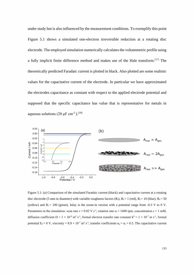
133
under study but is also influenced by the measurement conditions. To exemplify this point
Figure 5.1 shows a simulated one-electron irreversible reduction at a rotating disc
electrode. The employed simulation numerically calculates the voltammetric profile using
a fully implicit finite difference method and makes use of the Hale transform.[17] The
theoretically predicted Faradaic current is plotted in black. Also plotted are some realistic
values for the capacitative current of the electrode. In particular we have approximated
the electrodes capacitance as constant with respect to the applied electrode potential and
supposed that the specific capacitance has value that is representative for metals in
aqueous solutions (20 μF cm-2 ).[18]
Figure 5.1: (a) Comparison of the simulated Faradaic current (black) and capacitative current at a rotating
disc electrode (5 mm in diameter) with variable roughness factors (Rf), Rf = 1 (red), Rf = 10 (blue), Rf = 50
(yellow) and Rf = 100 (green). Inlay is the zoom-in version with a potential range from -0.3 V to 0 V.
Parameters in the simulation: scan rate ν = 0.02 V s-1, rotation rate ω = 1600 rpm, concentration c = 1 mM,
diffusion coefficient D = 1 × 10⁻⁹ m2 s-1, formal electron transfer rate constant k0 = 1 × 10⁻⁷ m s-1, formal
potential Ef = 0 V, viscosity = 8.9 × 10⁻⁷ m2 s-1, transfer coefficients αa = αc = 0.5. The capacitative current
-1.0 -0.8 -0.6 -0.4 -0.2 0.0
-0.16
-0.14
-0.12
-0.10
-0.08
-0.06
-0.04
-0.02
0.00
0.02
-0.3 -0.2 -0.1 0.0-12
-10
-8
-6
-4
-2
0
2
Cu
rre
nt
/
A
Potential / V
Cu
rrent / m
A
Potential / V
(a)
134
Icap = Cdl (20 μF cm-2) × Rf × Ageo × ν. (b) Schematic of electrode surface with different roughness factors.
The roughness factor Rf = the real electrode area (Areal) / the geometric area (Ageo).
To calculate the total electrode area we have multiplied the simulated geometric electrode
(Ageo / m2) area by a roughness factor, Rf, so that Areal = Ageo × Rf. As discussed later, for
heterogeneous electrode surfaces another important quantity is the roughness factor
which accounts only for the real area of the catalyst (Rf,catalyst). As outlined schematically
in Figure 5.1 b) in the present example a perfectly atomically flat electrode would have a
roughness factor of unity; a very well prepared polycrystalline electrode may be expected
to have a roughness factor of ~1.5[15] and a thin-film modified RDE will have a widely
variable roughness factor in the range of 10-1000. Thin-film modified electrodes find
routine use in electrocatalyst experiments,[15] where a catalyst is mixed with a non-
catalytic conductive support such as a form of nano-carbon and added as a thin-layer
across the surface of the electrode. The capacitative charging of the carbon support and
the catalyst will both contribute to the total background charging currents. As can be seen
in the guidelines provided by Kocha et al.[15] in their experiments for a thin-film modified
RDE of diameter 5 mm the total background currents are of the order of 15 μA, this
corresponds to an effective roughness factor of approximately 190.
From Figure 5.1 a) we can see that if we define the onset potential in this model case as
when the Faradaic current is expected to be equal in magnitude to the capacitative
contribution then the potential at which this cross over occurs is extremely sensitive to the
capacitance of the electrode. Even in this idealized case the value of the onset potential
135
varies by more than 200 mV for these realistic electrode capacitances. We further
comment that the definition of the capacitance as being a constant, as is implied in the
original editorial text, and as is used above is an over-simplification.[19]
5.5 What is the appropriate Tafel region of the current-potential
plot of a half-cell reaction in which to analyse a ‘Tafel slope’?
It is preferable to define a current range relative to the limiting steady state value as
opposed to defining a suitable potential range for meaningful Tafel analysis giving either
a transfer coefficient or, equivalently, a ‘Tafel slope’. The analysis provided here
indicates that provided a suitable background subtraction to remove the capacitative
current contribution is first performed then the current in the range between 10-80% of
the limiting current is suitable for kinetic analysis once a mass-transport correction has
been made. If the latter correction is neglected only currents below ~20% of the steady-
state current are suitable for use.
As described in Chapter 4, in a Tafel plot, the log of the current, log10|i|, is plotted against
the applied potential, E. If we assume the reaction is fully irreversible and well described
by the Tafel equation (Equation 5.12) then we can see for a one-electron transfer process
that such a semi-log plot will have a slope that is equal to −𝛼𝐹/(𝑅𝑇 × 𝑙𝑛10) and an
intercept (at zero overpotential, 𝜂𝑓) equal to 𝑙𝑜𝑔10(𝐹𝐴𝑘0𝑐𝐴). Originally electrocatalysis
experiments were performed using a form of current-interrupt technique known as the
commutator method.[20] Here a desired current density was driven to occur on a working
136
electrode, the cell was subsequently disconnected and the rapidly changing cell potential
measured against a reference cell. Measurement of the potential of the disconnected cell
as a function of the disconnection time allowed the original cell potential to be inferred
by extrapolation. Hence in reporting data in terms of current/potential graphs on the y-
axis the potential (the measured variable) was plotted against the current (the controlled
variable).[20b] Modern experiments tend to be performed potentiometrically and hence one
might expect the axes of the Tafel plot to be swapped, this is virtually never the case; old
habits die hard.
A linear Tafel plot of log10|i| vs E requires that, on the basis of Equation 5.6, the process
is fully irreversible and that the surface concentrations of the electroactive species remain
constant throughout the potential range of analysis. In practice the replenishment of the
active species via diffusion is slow and distortions arise from mass-transport limitations.
Consequently, it is necessary to ‘correct’ for these changes in the redox active species at
the electrode surface. The rotating disc electrode is to a reasonable approximation[22]
uniformly accessible. Consequently a plot of log10(1/I - 1/Ilim) against the applied
potential allows for these changes in the surface concentration of the redox active species
during the course of the scan to be suitably accounted for. The need to make a mass-
transport correction has long been advocated.[23]
Figure 5.2 plots an example mass-transport corrected Tafel plot for a simulated RDE
experiment. In this simulation we have assumed that the total current can be expressed
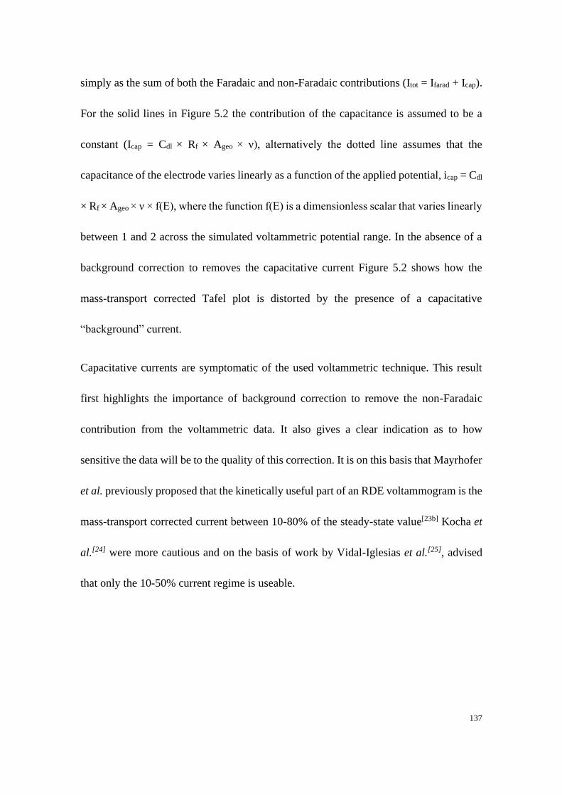
137
simply as the sum of both the Faradaic and non-Faradaic contributions (Itot = Ifarad + Icap).
For the solid lines in Figure 5.2 the contribution of the capacitance is assumed to be a
constant (Icap = Cdl × Rf × Ageo × ν), alternatively the dotted line assumes that the
capacitance of the electrode varies linearly as a function of the applied potential, icap = Cdl
× Rf × Ageo × ν × f(E), where the function f(E) is a dimensionless scalar that varies linearly
between 1 and 2 across the simulated voltammetric potential range. In the absence of a
background correction to removes the capacitative current Figure 5.2 shows how the
mass-transport corrected Tafel plot is distorted by the presence of a capacitative
“background” current.
Capacitative currents are symptomatic of the used voltammetric technique. This result
first highlights the importance of background correction to remove the non-Faradaic
contribution from the voltammetric data. It also gives a clear indication as to how
sensitive the data will be to the quality of this correction. It is on this basis that Mayrhofer
et al. previously proposed that the kinetically useful part of an RDE voltammogram is the
mass-transport corrected current between 10-80% of the steady-state value[23b] Kocha et
al.[24] were more cautious and on the basis of work by Vidal-Iglesias et al.[25], advised
that only the 10-50% current regime is useable.
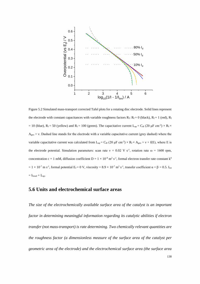
138
Figure 5.2 Simulated mass-transport corrected Tafel plots for a rotating disc electrode. Solid lines represent
the electrode with constant capacitances with variable roughness factors Rf: Rf = 0 (black), Rf = 1 (red), Rf
= 10 (blue), Rf = 50 (yellow) and Rf = 100 (green). The capacitative current Icap = Cdl (20 μF cm-2) × Rf ×
Ageo × ν. Dashed line stands for the electrode with a variable capacitative current (grey dashed) where the
variable capacitative current was calculated from Icap = Cdl (20 μF cm-2) × Rf × Ageo × ν × f(E), where E is
the electrode potential. Simulation parameters: scan rate ν = 0.02 V s-1, rotation rate ω = 1600 rpm,
concentration c = 1 mM, diffusion coefficient D = 1 × 10⁻⁹ m2 s-1, formal electron transfer rate constant k0
= 1 × 10⁻⁷ m s-1, formal potential Ef = 0 V, viscosity = 8.9 × 10⁻⁷ m2 s-1, transfer coefficient α = = 0.5. Itot
= Ifarad + Icap.
5.6 Units and electrochemical surface areas
The size of the electrochemically available surface area of the catalyst is an important
factor in determining meaningful information regarding its catalytic abilities if electron
transfer (not mass-transport) is rate determining. Two chemically relevant quantities are
the roughness factor (a dimensionless measure of the surface area of the catalyst per
geometric area of the electrode) and the electrochemical surface area (the surface area
1 2 3 4 5 6
0.0
0.1
0.2
0.3
0.4
0.5
0.6
80% Id
50% Id
Ove
rpo
ten
tia
l (v
s E
f) / V
log10(1/I - 1/Ilim) / A
10% Id
139
of the catalyst per gram of catalyst). Measurement of the real surface area of the catalyst
is often experimentally challenging and is in some cases sensitive to how the measurement
is made.
D. Voiry et al.[1] present both the electrochemical surface area (ECSA) and the turnover
frequency (TOF) as dimensionless parameters! In the guidelines the ECSA is given as the
dimensionless ratio of the specific double layer capacitance (Cdl) relative to a given
reference surface specific capacitance, this definition seems to follow a previous article
in ACS Catalysis.[26] Similarly the TOF is given as “nproduct / nsite”;[1] how these two terms
(nproduct and nsite) should be defined and measured is left to the reader. We note as follows,
first, D. Voiry et al. have interpreted the ECSA as a roughness factor with a subsequent
confusing conflation of terminology in the text. Second, we comment that it is essential
for a surface area to contain the unit of length squared; similarly a quantity labelled as a
“frequency” has units of reciprocal time. As a consequence of these non-conventional
definitions some of the derived expressions provided D. Voiry et al. may also be usefully
reconsidered.
In the literature the definition of the ECSA may vary depending on the context in which
it is being used; however, following the ORR field the ECSA is probably most usefully
defined as the area of the catalyst per gram of material (m2 gcatalyst−1 ).[23b] This value in
combination with the specific activity of the catalyst (A mcatalyst−2 , the catalytic Faradaic
current in Ampere per catalyst area), yields the mass activity for the material (A gcatalyst−1 ).
140
These latter two values vary as a function of potential. Consequently to get a relative
measure of activity these values are often reported at a given potential. It is the value for
the mass activity that most directly translates to the cost of a platinum based fuel cell
device.[27] But in terms of physico-chemical insight the important factor is arguably the
specific activity of the catalyst. This value of the catalysts specific activity gives a
measure of the rate of reaction per unit area of the catalyst, accurate determination of the
magnitude of this value is not necessarily as facile as it may seem; this is especially true
if the catalytic surface is not uniformly accessible as is the case for porous electrode
surfaces. Related to these values is the (dimensionless) catalyst roughness factor, this
value is the surface area of the catalyst per geometric area of the electrode. In some
contexts the roughness factor may also, vide supra, refer to the total surface area of the
electrode relative to its geometric area.
The measurement of the surface area of the catalysts is not necessarily straightforward.
Note that “best practice” documents in the field of ORR tend to only very briefly[15], if at
all[23b], mention that such electrode capacitance measurements (or the measurement of
other surface processes such as the under-potential deposition of hydrogen) need to be
made using an analog[28] potentiostat. In the case of measuring platinum electrochemical
surface areas, major errors can be made if staircase voltammetry is used and, of course,
almost all modern commercial potentiostats provide staircase voltammetry as the default
technique, so this can lead to the underestimation of the platinum surface area and will
hence cause an overestimation regarding the material’s specific activity. As an aside
141
similar issues arise with protein film voltammetry.[29] This issue with staircase
voltammetry is often covered in potentiostat manuals;[30] but who reads a manual?[31]
5.7 Conclusions
Six topics have been discussed from electrochemical perspective. Some of the above is
opinion and others in the field may dispute aspects of it. Many comments will be obvious
to those in the electrochemical field but it is hoped that this chapter has clarified some of
the important points.
References:
[1] D. Voiry, M. Chhowalla, Y. Gogotsi, N. A. Kotov, Y. Li, R. M. Penner, R. E. Schaak, P. S. Weiss,
ACS Nano 2018, 12, 9635-9638.
[2] D. Li, C. Batchelor-McAuley, R. G. Compton, Applied Materials Today 2020, 18.
[3] X. Jiao, C. Batchelor-McAuley, E. Katelhon, J. Ellison, K. Tschulik, R. G. Compton, The Journal
of Physical Chemistry C 2015, 119, 9402-9410.
[4] E. Wilhelm, R. Battino, R. J. Wilcock, Chemical reviews 1977, 77, 219-262.
[5] Note the formal potential is still relevant for understanding the thermodynamics of electrochemical
processes involving dissolved gases.
[6] E. R. Cohen, I. Mills, C. Royal Society of, T. Cvitas, P. International Union of, P. Applied
Chemistry, D. Biophysical Chemistry, J. G. Frey, M. Quack, B. Holström, K. Kuchitsu, R.
Marquardt, Quantities, Units and Symbols in Physical Chemistry, Royal Society of Chemistry,
2007.
[7] T. Erdey-Grúz, M. Volmer, Zeitschrift für physikalische Chemie 1930, 150, 203-213.
[8] In strict accordance with IUPAC k0 as defined here is the formal electrochemical rate constant as
the used reference potential is the formal not the standard potential see ref 6.
[9] H. Eyring, S. Glasstone, K. J. Laidler, The Journal of Chemical Physics 1939, 7, 1053-1065.
[10] N. Pentland, J. M. Bockris, E. Sheldon, Journal of The Electrochemical Society 1957, 104, 182-
194.
[11] S. Trasatti, Journal of Electroanalytical Chemistry and Interfacial Electrochemistry 1972, 39,
163-184.
[12] W. Thomson, Transactions of the Royal Society of Edinburgh 1853-1857, 21, 123-171.
[13] L. Meites, P. Zuman, H. W. Nurnberg, in Pure and Applied Chemistry, Vol. 57, 1985, p. 1491.
142
[14] For more information on this additonal mass-transport correction to the predicted half-wave
potential, the reader is directed towards ref 3. In the SI of this reference the additionally required
correction for the half-wave potential is derived (Equation 12 of SI in ref.3), simply requiring the
definition for the hydrodynamic layer thickness to be substituted into this expression.
[15] S. S. Kocha, K. Shinozaki, J. W. Zack, D. J. Myers, N. N. Kariuki, T. Nowicki, V. Stamenkovic,
Y. Kang, D. Li, D. Papageorgopoulos, Electrocatalysis 2017, 8, 366-374.
[16] A. Maljusch, E. Ventosa, R. A. Rincón, A. S. Bandarenka, W. Schuhmann, Electrochemistry
Communications 2014, 38, 142-145.
[17] aR. G. Compton, E. Laborda, K. R. Ward, Understanding Voltammetry: Simulation Of Electrode
Processes, World Scientific Publishing Company, 2013; bJ. M. Hale, Journal of Electroanalytical
Chemistry (1959) 1963, 6, 187-197.
[18] B. B. Damaskin, A. N. Frumkin, Electrochimica Acta 1974, 19, 173-176.
[19] H. Gerischer, R. McIntyre, D. Scherson, W. Storck, Journal of Physical Chemistry 1987, 91, 1930-
1935.
[20] aE. Newbery, Journal of the Chemical Society, Transactions 1914, 105, 2419-2435; bF. P.
Bowden, a. E. K. Rideal, Proceedings of the Royal Society 1928, 120, 59.
[21] D. Li, C. Lin, C. Batchelor-McAuley, L. Chen, R. G. Compton, Journal of Electroanalytical
Chemistry 2018, 826, 117-124.
[22] aJ. Newman, Journal of the Electrochemical Society 1966, 113, 1235-1241; bW. H. Smyrl, J.
Newman, Journal of The Electrochemical Society 1971, 118, 1079-1081.
[23] aW. J. Albery, Electrode kinetics, Clarendon Press, 1975; bK. J. J. Mayrhofer, D. Strmcnik, B. B.
Blizanac, V. Stamenkovic, M. Arenz, N. M. Markovic, Electrochimica Acta 2008, 53, 3181-3188.
[24] K. Shinozaki, J. W. Zack, R. M. Richards, B. S. Pivovar, S. S. Kocha, Journal of the
Electrochemical Society 2015, 162, F1144-F1158.
[25] F. J. Vidal-Iglesias, J. Solla-Gullón, V. Montiel, A. Aldaz, Electrochemistry Communications
2012, 15, 42-45.
[26] E. L. Clark, J. Resasco, A. Landers, J. Lin, L.-T. Chung, A. Walton, C. Hahn, T. F. Jaramillo, A.
T. Bell, ACS Catalysis 2018, 8, 6560-6570.
[27] A. Kongkanand, M. F. Mathias, The journal of physical chemistry letters 2016, 7, 1127-1137.
[28] C. Batchelor-McAuley, M. Yang, E. M. Hall, R. G. Compton, Journal of Electroanalytical
Chemistry 2015, 758, 1-6.
[29] H. A. Heering, M. S. Mondal, F. A. Armstrong, Analytical chemistry 1999, 71, 174-182.
[30] M.-. Autolab, pp. https://www.metrohm.com/en-gb/applications/AN-EC-007.
[31] R. G. Alethea L. Blackler, Vesna Popovic and M. Helen Thompson, 2018.
143
Chapter 6
Electrochemical Measurement of the Size of Microband
Electrodes: A Theoretical Study
Microband electrodes are popular in various applications, especially in sensors, since they
have some of the advantages of both macro- and micro-electrodes. This work first briefly
introduces the fabrication methods reported for both single microband electrodes and
arrays and their uses in sensing applications. A theoretical section on band electrodes
provides background information on the structure of band electrodes, their diffusional
profiles and the types of voltammetric behaviour observed. Furthermore, due to the
difficulties in measuring the dimensions of band electrodes, a theoretical proof-of-
concept study demonstrating the use of an electrochemical method to measure the width
and length of a band electrode of unknown dimensions is presented. It is found that by
using a fully irreversible redox couple it is possible to characterise a band electrode
without prior knowledge of the electron transfer rate constant or the formal potential. By
using the peak-to-peak separation (Ep-p) and the magnitude of the ratio of backward peak
current to forward peak current (|Ibackward/Iforward|) as diagnostic parameters, the band width
can be estimated with an error of less than 4% compared to its true value and with an
error in length of less than 1%.
144
This work presented in this chapter consists of two first author papers which have been
published in Journal of Electroanalytical Chemistry[1] and ACS Sensors[2], respectively.
6.1 Introduction
6.1.1 Background overview
Microelectrodes have, since the 1980s, attracted a lot of attention, providing new
possibilities in both fundamental studies and applications, but most notably in sensors.
The International Union of Pure and Applied Chemistry (IUPAC) has defined that a
microelectrode has dimensions of tens of micrometres or less, down to the submicrometre
range[3] whereas other terms, for example, ultramicroelectrodes and nanoelectrodes, are
sometimes used in the literature to describe electrodes with dimensions less than
micrometre scale. Decreasing the size of an electrode to the micron or sub-micron scale
alters the voltammetric behaviour offering a number of advantageous properties over
conventional macroelectrodes.[3-4] First, higher current densities are obtained due to the
enhanced mass transport.[4a, 4c] Second, ohmic resistance effects decrease due to the
smaller electrode size.[4a, 5] Third, microelectrodes have smaller capacitances which
increases the signal-to-background ratio and improves the response time of the system.
Furthermore, due to their sizes they can be applied in the measurements with samples
with small volumes in, for example, medical and biological research.[6] Although the
advantages of microelectrodes are clearly apparent, one drawback of the use of a single
micro- or nano-disc electrode is the low absolute current output; the measured currents

145
are often in the nano to sub-nanoampere range. Consequently, the current measurement
is sensitive to issues of electrical noise, often necessitating the use of a Faraday cage. This
requirement for electrical shielding can negatively impact their applications in real world
sensing devices. Micro- or nanoelectrodes with a band geometry, where the electrical
interface is micro- or nanoscopic in one dimension and macroscopic in the other, can
address this problem of sensitivity to electrical noise; a larger current output can be
produced by simply having a longer band. In addition, the total current output can also be
increased by using multiple single bands operated in parallel. These so-called band arrays
can offer the same sensitivity as a single band electrode but with added benefits including
higher total current output and less susceptibility to interference.
Micro- to nanoband electrodes and their arrays have been fabricated as chemical sensors[7]
or biosensors[8]. Sensors are widely used in various fields for example in food processing,
medical fields, environmental field, where some of criteria need to be taken into
consideration for the sensor design and fabrication: 1) high sensitivity and selectivity; 2)
low limit of detection (LOD); 3) ease of fabrication.[9] The first two requirements can be
realised due to the above mentioned advantages of microbands (arrays), leading to an
improved signal-to-noise ratio and hence improved sensitivity and lower detection limit.
Additionally microband arrays own the advantages of easy fabrication compared to
microelectrode arrays with other geometries and hence provide more possibilities in
applications. Important examples of the use of band electrodes for analytical applications
include the development of a chemical sensor based on screen printed carbon microband
146
electrodes requiring no further chemical modification to give a low detection limit for the
determination of Pb2+.[7c] A boron-doped diamond band electrode for use in end-column
amperometric detection with enhanced sensitivity and lower noise level for several
groups of important analytes (e.g. nitroaromatic explosives, phenols) on capillary
electrophoresis microchips has been reported.[10] More recently, a capacitative biosensor
with a high sensitivity and a wide dynamic detection range was fabricated using a
commercialised gold interdigitated electrode array the surface of which was
functionalised with 24-nucleotide DNA probes to detect DNA molecules.[11]
Beyond being of analytical value band electrodes are also of importance in fundamental
research. The decreased resistance and capacitance of such electrode designs offer the
possibility of investigating fast electrochemical reaction mechanisms and exploring
electrochemical reactions in organic solvents with low permittivity such as toluene.[12]
Another recent example of fundamental work is that by Zhang et al. who reported the use
of gold nanoband electrodes to study the motion of silver nanoparticles.[13] Li et al.
measured the resistance across individual carbon nanotubes in contact with and bridging
across an interdigitated gold band electrode array.[14] These wide and varied uses of
micro- or nano-band electrodes encourage the investigation of reproducible fabrication
methods for making thinner band electrodes or electrodes made of different materials.
147
6.1.2 Fabrication methods
Generally single band electrodes are fabricated in a “sandwich” configuration, where a
sheet of an electrode material is sandwiched between two insulating layers and the stack
cut in a direction perpendicular to the sheet, exposing a band of the electrode material.
The electrode materials are first deposited onto the insulating substrate using various
methods, which, for example, include sputtering[5] or thermal vapour evaporation[5, 10, 15].
A second insulating layer is then either mechanically covered or surface printed (e.g.
screen printing[7c, 7d, 16] or photolithography[17]) on top of the band layer. Metals, especially
gold and platinum, are the most commonly used materials as the band layer to construct
band electrodes because of their relatively wide commercial availability as thin sheets or
foils of high purity.[18] Moreover, thin metal films can be obtained by sputtering or
evaporation, which are usually applied during lithographic fabrication methods. Other
materials such as graphite, carbon nanotubes (CNTs) and doped diamond have been used
as electrode materials. In terms of the deposition method of the insulating layer, the
fabrication methods can be categorised into two: “mechanical fabrication” and “surface
printed fabrication”.
6.1.2.1 Mechanical fabrication for single bands
This method is relatively simple and involves the mechanical sealing of a band layer
between insulating layers which are normally commercially available, for example,
microscope glass slides[5, 19], Mylar sheets[5] etc. The resulting electrodes are exposed by
148
polishing or cutting one edge of the electrode. For instance, single Pt microband
electrodes with thicknesses of 5-20 μm were first constructed using the sandwich method
by Wightman and co-workers where the platinum band was fabricated by sealing a thin
platinum sheet in soft glass with a flame and one of the edge was exposed by polishing.[20]
Electrical contact was achieved using silver epoxy with a conductive metal wire. The
approximate thicknesses of Pt band electrodes were determined via the use of an optical
microscope.[20] Apart from using commercially available metal sheets as the “filling” of
the sandwich, metal nanoscopic band electrodes have also been fabricated using vapour
deposition or sputtering on different substrates with the thickness of the metal film
controlled by the deposition time. For example, gold and platinum nanoband electrodes
with thicknesses of lower to 30 nm were fabricated by sputtering metal film onto a glass
microscope slide, which was covered with another glass slide.[5] Carbon-based materials,
such as graphite[5, 7d, 20] and CNTs[21] have also been fabricated into band electrodes. A
graphite microband electrode was fabricated by sealing a thin sheet of graphite from the
basal plane of a block of pressure-annealed pyrolytic graphite between two layers of heat-
bondable plastic at 260 oC for 18 mins.[20] The direct measurement of the band width was
attempted but the electron micrographs of graphite band electrode showed that parts of
graphite surface were occluded by the plastic bonding material and hence the accurate
measurement of band was considered impossible.[20]
149
6.1.2.2 Surface printed fabrication methods for single bands
Band electrodes fabricated using this method also have the ‘sandwich’ configuration but
all layers are deposited using screen printing techniques. This allows scale up of the
fabrication process. The fabrication of single screen-printed carbon microband electrodes
has been reported by Williams and co-workers[22]. Here, a line of a suitable commercial
conductive ink (Pt, Au, C etc.) was printed 2-8 mm wide and ~10 μm thick onto the
surface of alumina tiles, followed by another coating layer of dielectric material.[22a] The
corresponding platinum, gold and carbon band electrode was obtained by cutting
perpendicularly to the direction of the line and a fresh surface could be obtained by
snapping along a pre-scribed line.[22a] A more recent screen printed graphite microband
electrode was reported by Banks and co-workers for the sensing of NADH and nitrite.[7d]
A commercial carbon-graphite ink was screen printed onto a polyester flexible film, cured
and the silver/silver chloride reference electrode was attached by screen printing Ag/AgCl
paste onto the substrate.[7d] The whole surface was finally covered with a printed dielectric
ink.[7d]
6.1.2.3 Fabrication of band arrays
A band electrode array which consists of multiple single bands can have different
arrangements, for example, a regular band array with parallel alignments or a regular band
array with an interdigitated arrangement. Band electrode arrays are mostly fabricated
using surface printed method such as lithographic techniques due to the good
150
reproducibility. However, for “mini-arrays” which only consist of several single bands,
sandwich-type band electrodes are made using the mechanical fabrication method. Dual
or triple band electrodes are ‘mini-arrays’ comprised of just two or three single bands
positioned in parallel. These electrodes can be fabricated as multiple layers of
sandwiches[19b, 23], of which the fabrication method is similar to the sandwich-type single
band but with multiple layers. Bard and co-workers fabricated such closely spaced
ultramicroband electrodes with effective thicknesses of 0.01-6 μm by sputter deposition
of Pt onto both slides of 2 to 12 μm thick mica sheets that were mounted between glass
slides.[23d] On the other hand, microband arrays with multiple single bands are often
produced using surface printed method, in which case lithographic techniques[17a, 24] are
the most frequently applied. The lithographic technology can effectively pattern and build
thin film electrode materials, for example, platinum and gold on substrates with well-
defined and reproducible dimensions. Dobson and co-workers fabricated a 13-microband
channel flow electrode array, with electrodes ranging in size from the milimeter to the
submicrometer scale using standard semiconductor processing methods.[24d, 25] This
channel electrode array was used as a probe of mechanism and kinetics of complex
electrode processes.[24d]
Band electrodes with a submicrometer width can be characterised using Optical
Microscopy or Scanning Electron Microscopy (SEM)[7e, 8d]. However, the successful use
of SEM requires a clear contrast between the materials of the band and the external
insulating layers. Microdisc electrodes are routinely sized and characterised
151
voltammetrically where the magnitude of a steady-state diffusional current is used to
calibrate the efficient electrode radius. For a microband electrode, rather than a single
radius, there are two unknowns – the length and the width. An electrochemical method is
described below to provide a general and easy approach for general use to calibrate the
size of the unknown electrode.
Accurate electrode sizing measurements using a voltammetric method requires the
appropriate choice of the electroactive redox couple to be used. Since a redox couple
involving the transfer of multiple electrons would offer mechanistic complexity, fully
reversible or irreversible redox couples which undergo single electron transfer are
preferred. In particular well characterised standard redox couples such as Ru(NH3)62+/3+
and Fe(CN)63-/4- are often used to calibrate the size of both macroelectrodes and
microelectrodes due to their well-known diffusion coefficients[8b]. The voltammetric
behaviour of a band electrode has been studied using such standard redox couples[7e, 26];
however, the electrochemical characterisation of the electrode dimensions has not been
attempted. The following reports a home-written simulation method developed
specifically for a single microband electrode with the expectation that the dimensions of
a band electrode can be characterised by comparing experimental and simulated
voltammograms by analysing the kinetic information obtained from independent
experiments. Note that the simulations are rigorous and do not depend on analogies being
made between cylinders and bands.
152
Electrode processes in both the reversible and irreversible limits are considered. On the
one hand, for a fully reversible one electron transfer process, knowledge of the electrode
kinetics (standard rate constant and transfer coefficient) is not needed. The formal
potential (Ef) can be estimated as the mid-point potential of forward and backward peak
potentials (Ep(forward) and Ep(backward)) in a conventional linear diffusional cyclic
voltammogram. Conversely, using a fully irreversible redox couple requires that the
kinetic parameters are known. However, the transfer coefficient can be easily calculated
from Tafel analysis using a Tafel region corresponding to 1% to 30% of the peak current[9].
In both cases, the value of diffusion coefficient of the electroactive species can be found
in the literature or measured using a microdisc electrode from steady-state voltammetry[7e,
26]. In the following, we develop a theoretical study showing the viability of the method
and establish the requirements of the optimal redox couple for microband sizing to
facilitate subsequent experiments. Thus, this theoretical study validates how simple
voltammetric measurements can be used to characterise the length and width of a band
electrode based on the use of a home-written programme by Dr Chuhong Lin.
6.2 Background theory
6.2.1 General theory background on band electrodes
For a molecule freely diffusing in solutions the mean squared distanced travelled <X2>
in a time t can be expressed by the following equation (Equation 6.1):
153
< 𝑋2 >= 2𝐷𝑡 (6.1)
where D is the diffusion coefficient of the species. For a molecular species in aqueous
solution at 25 oC the diffusion coefficient is often in the range of 0.1 - 10 × 10-9 m2 s-1,
moreover most dynamic electrochemical experiments last between one and a few tens of
seconds. Consequently, during the course of most voltammetric measurements the
molecules in solution will have travelled on average between 10-1000 microns. This
average distance travelled relative to the size of the electrode is important in determining
the diffusion profile to an interface. When <X2>0.5 is small compared to the length scale
of the electrode, the mass-transport to the interface is linear. Conversely when <X2>0.5 is
large compared to the electrode length scale the mass-transport to the interface is
convergent. The operative mass-transport regime controls the voltammetric response of
the solution phase species at an electrode.
Chronoamperometry and cyclic voltammetry are two widely used techniques in
electroanalysis. During the course of the experiment the characteristic distance travelled
by a molecule varies as a function of time, as described by Equation 6.1. Hence, during
the course of the chronoamperogram the diffusion profile will evolve; consequently, as
with the current response at other electrode geometries, there is no simple expression for
describing the variation of the mass-transport limited current as a function of time.
However, the most commonly used result describing the chronoamperometric response
for this band electrode geometry for a simple one electron oxidation or reduction, A ± e
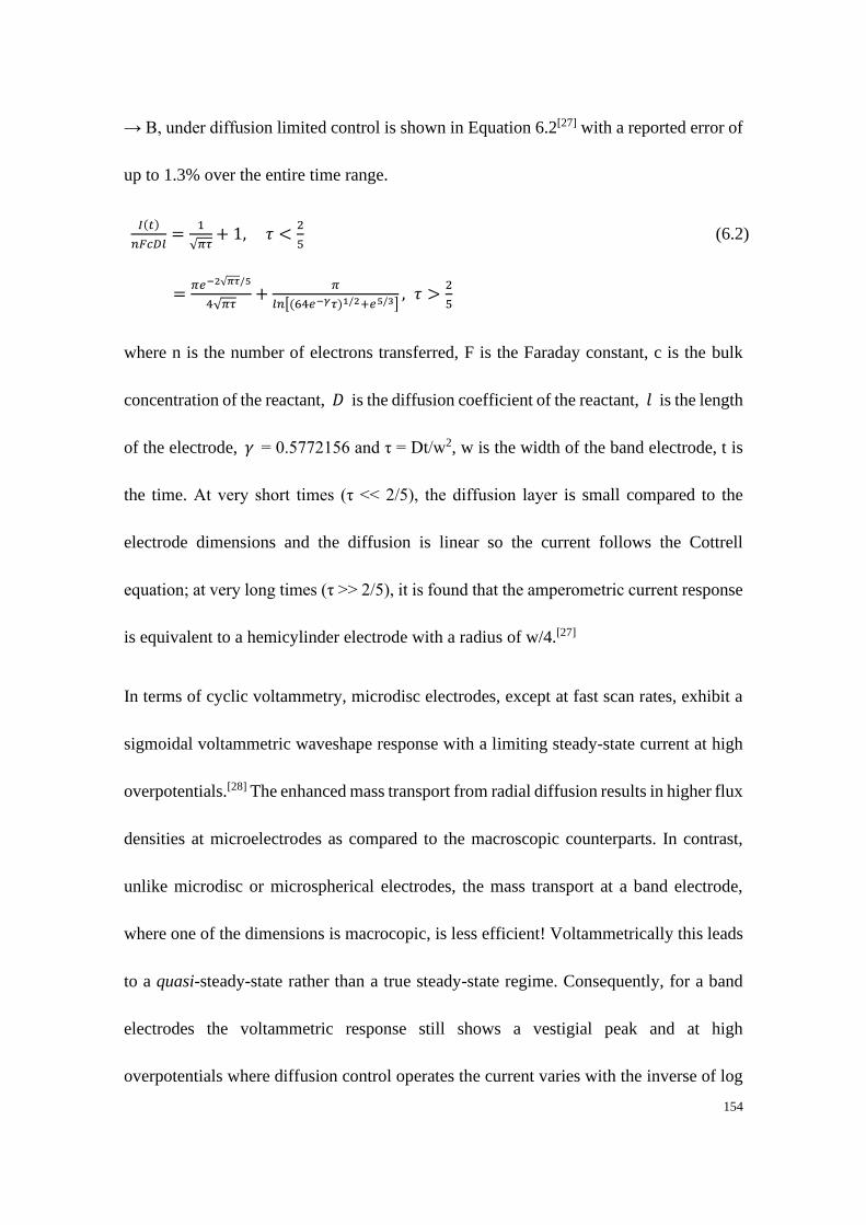
154
→ B, under diffusion limited control is shown in Equation 6.2[27] with a reported error of
up to 1.3% over the entire time range.
𝐼(𝑡)
𝑛𝐹𝑐𝐷𝑙=
1
√𝜋𝜏+ 1, 𝜏 <
2
5 (6.2)
=𝜋𝑒−2√𝜋𝜏/5
4√𝜋𝜏+
𝜋
𝑙𝑛[(64𝑒−𝛾𝜏)1/2+𝑒5/3], 𝜏 >
2
5
where n is the number of electrons transferred, F is the Faraday constant, c is the bulk
concentration of the reactant, 𝐷 is the diffusion coefficient of the reactant, 𝑙 is the length
of the electrode, 𝛾 = 0.5772156 and τ = Dt/w2, w is the width of the band electrode, t is
the time. At very short times (τ << 2/5), the diffusion layer is small compared to the
electrode dimensions and the diffusion is linear so the current follows the Cottrell
equation; at very long times (τ >> 2/5), it is found that the amperometric current response
is equivalent to a hemicylinder electrode with a radius of w/4.[27]
In terms of cyclic voltammetry, microdisc electrodes, except at fast scan rates, exhibit a
sigmoidal voltammetric waveshape response with a limiting steady-state current at high
overpotentials.[28] The enhanced mass transport from radial diffusion results in higher flux
densities at microelectrodes as compared to the macroscopic counterparts. In contrast,
unlike microdisc or microspherical electrodes, the mass transport at a band electrode,
where one of the dimensions is macrocopic, is less efficient! Voltammetrically this leads
to a quasi-steady-state rather than a true steady-state regime. Consequently, for a band
electrodes the voltammetric response still shows a vestigial peak and at high
overpotentials where diffusion control operates the current varies with the inverse of log
155
of the experimental time.[29] In the limit where the width of the band is microscopic in
dimensions, the magnitude of the voltammetric response is relatively insensitive to the
width of the band. Here the voltammetric peak current is approximately proportional to
the length of the electrode and the electrode width to the power of ~0.15.[30] This relative
insensitivity to the electrode width is shown in Figure 6.1, where the current only
increases by a factor of ~1.3 as the band width increases by a factor of 8. The inlay in
Figure 6.1 shows the linear relationship between the logarithm of peak current and the
logarithm of the band width with a gradient close to 0.15[30].
Figure 6.1 Simulated voltammograms on single band electrodes with various band widths: w = 100 nm
(red), w = 200 nm (blue), w = 400 nm (yellow) and w = 800 nm (black). Parameters used in the simulations:
D = 1 × 10⁻⁹ m2 s-1, k0 = 1 × 10⁻⁷ m s-1, Ef = 0 V, cbulk = 1 mM, αa = αc = 0.5, length = 0.1 cm. The inlay
shows the plot of the logarithm of the peak current as a function of the logarithm of band width. The linear
relationship gives a gradient of 0.16.
A band array comprises of multiple single bands which are positioned in parallel as
schematically shown in Scheme 6.1(a). The bands are microscopic in the x-direction
156
(band width) but macroscopic in the y-direction (length).[31] The inter-band separation is
the distance between the centres of two adjacent bands in the x-direction. When multiple
band electrodes are packed in parallel, unlike the diffusion profile at a single band, the
diffusion fields from adjacent bands may interfere and compete with each other. The
situation can be summarised into four diffusional categories as defined by Davies et al.[4c]
which are shown in Scheme 6.1 (b)[32] and the corresponding voltammograms, at the fully
irreversible limit, are shown in Figure 6.2. These voltammograms were simulated using
a home-written microband programme by Dr Chuhong Lin where the diffusional regime
which is operative depends on a number of factors including, the band width w, the inter-
band separation δinter-band, the molecular species diffusion coefficient D and the
experimental time t (as often controlled by the voltammetric scan rate).[33] In category 1
which corresponds to very short times, the diffusion layer thickness is much smaller
compared to the band width and band separation and the mass transport is dominated by
linear diffusion. Here the magnitude of the voltammetric response is proportional to the
total band area. In category 2 corresponding to longer times, the diffusion to each band is
convergent and due to the large band separation, each band behaves independently. The
measured total current equals to the collection of all isolated bands, where as discussed
previously the magnitude of the voltammetric response is relatively insensitive to the
electrode width. As is shown in Figure 6.2, the voltammetric behaviour on a band array
with a band width of 100 nm and an inter-band separation δinter-band of 300 µm (black
curve) is equivalent to that on a single microband electrode (gray curve) with a band width
157
of 100 nm at a scan rate of 0.025 V s-1. However, if the inter-band separation is smaller
the bands no longer remain diffusionally independent. Category 4 is the extreme of this
case where the diffusion profiles overlap so significantly that the diffusional profile to the
whole array becomes linear (red curve in Figure 6.3 with δinter-band of 0.3 µm) where the
diffusion fields completely overlap leading to a linear concentration profile towards the
entire array as a whole. The array then behaves the same as a macroelectrode with the
same geometric area as the entire array. Obviously this behaviour destroys some of the
benefits of using microelectrodes! Category 3 represents a transition between categories
2 and 4, where the diffusion fields overlap partially between adjacent bands, which
reduces the flux at the edge of the electrodes. Examples of this case are shown as green
and blue curves in Figure 6.2 where the inter-band separations δinter-band are 30 µm and 3
µm, respectively. Consequently, the highest sensitivity at a microband array (i.e. the
average current measured per band) can only be obtained in category 2 due to the rapid
diffusion at the band edge. The schematic shown in Scheme 6.1 focuses on regular spaced
band arrays[31], whilst the voltammetric responses at randomly distributed microband
arrays have been studied by Streeter et al.[32]

158
Scheme 6.1 (a) Schematic diagram of a section of a microband array. The theoretical array extends to
infinity in both x- and z-directions.[31] (b) Schematic diagrams of diffusion categories 1-4 at a microband
array.[32] Adapted with permission from refs [31] and [32]. Copyright © 2007 American Chemical Society.
Figure 6.2 Simulated voltammograms on a single microband (gray) and microband arrays with variable
inter-band separation (δinter-band) at the fully irreversible limit: δinter-band = 0.3 µm (red), 3 µm (blue), 30 µm
(green) and 300 µm (black). Inlay presents the zoom-in version of the voltammogram on the band electrode
with the δinter-band of 0.3 µm (red). Parameters used in the simulations: band width = 100 nm, D = 1 × 10 -9
m2 s-1, k0 = 1 × 10⁻⁷ m s-1, Ef = 0 V, cbulk = 1 mM, αa = αc = 0.5, length = 0.1 cm.
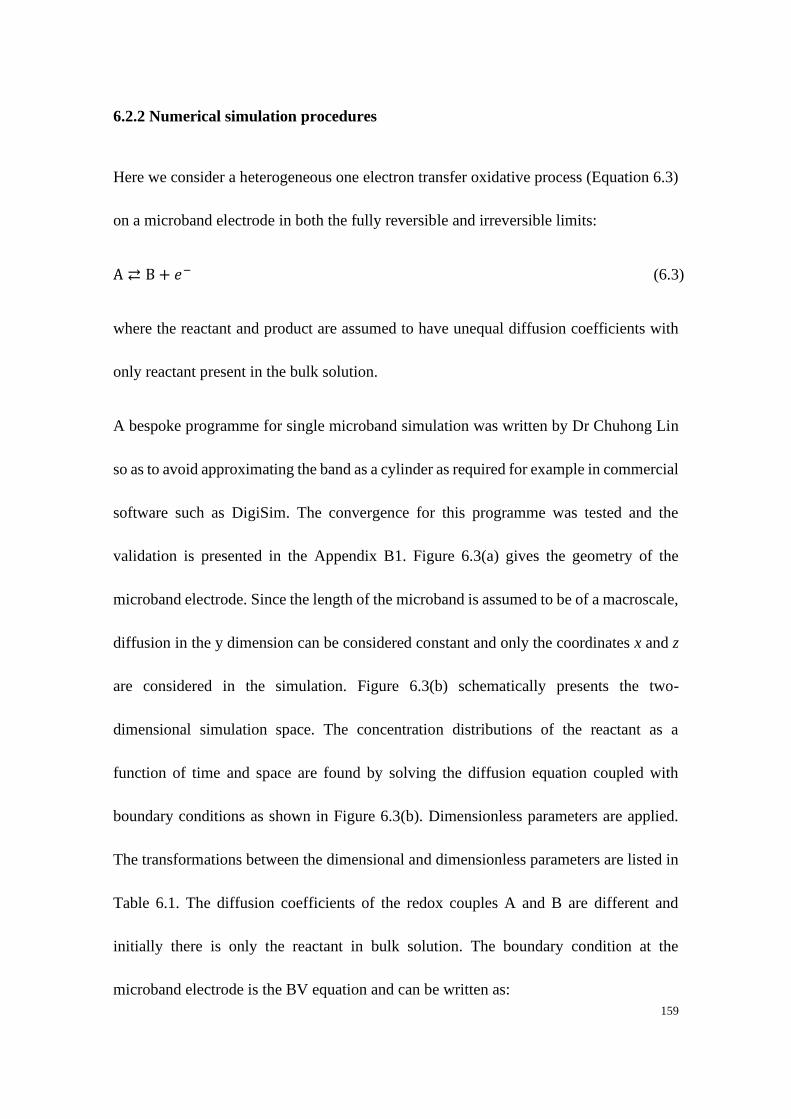
159
6.2.2 Numerical simulation procedures
Here we consider a heterogeneous one electron transfer oxidative process (Equation 6.3)
on a microband electrode in both the fully reversible and irreversible limits:
A ⇄ B + 𝑒− (6.3)
where the reactant and product are assumed to have unequal diffusion coefficients with
only reactant present in the bulk solution.
A bespoke programme for single microband simulation was written by Dr Chuhong Lin
so as to avoid approximating the band as a cylinder as required for example in commercial
software such as DigiSim. The convergence for this programme was tested and the
validation is presented in the Appendix B1. Figure 6.3(a) gives the geometry of the
microband electrode. Since the length of the microband is assumed to be of a macroscale,
diffusion in the y dimension can be considered constant and only the coordinates x and z
are considered in the simulation. Figure 6.3(b) schematically presents the two-
dimensional simulation space. The concentration distributions of the reactant as a
function of time and space are found by solving the diffusion equation coupled with
boundary conditions as shown in Figure 6.3(b). Dimensionless parameters are applied.
The transformations between the dimensional and dimensionless parameters are listed in
Table 6.1. The diffusion coefficients of the redox couples A and B are different and
initially there is only the reactant in bulk solution. The boundary condition at the
microband electrode is the BV equation and can be written as:
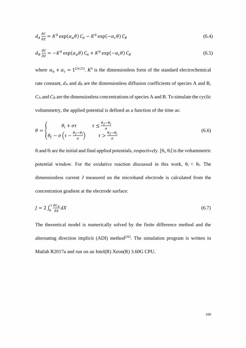
160
𝑑𝐴𝜕𝐶
𝜕𝑍= 𝐾0 exp(𝛼𝑎𝜃) 𝐶𝐴 − 𝐾0 exp(−𝛼𝑐𝜃) 𝐶𝐵 (6.4)
𝑑𝐵𝜕𝐶
𝜕𝑍= −𝐾0 exp(𝛼𝑎𝜃) 𝐶𝐴 + 𝐾0 exp(−𝛼𝑐𝜃) 𝐶𝐵 (6.5)
where 𝛼𝑎 + 𝛼𝑐 = 1[24,25]. K0 is the dimensionless form of the standard electrochemical
rate constant, dA and dB are the dimensionless diffusion coefficients of species A and B,
CA and CB are the dimensionless concentrations of species A and B. To simulate the cyclic
voltammetry, the applied potential is defined as a function of the time as:
𝜃 = {𝜃𝑖 + 𝜎𝜏 𝜏 ≤
𝜃𝑓−𝜃𝑖
𝜎
𝜃𝑓 − 𝜎 (𝜏 −𝜃𝑓−𝜃𝑖
𝜎) 𝜏 >
𝜃𝑓−𝜃𝑖
𝜎
(6.6)
θi and θf are the initial and final applied potentials, respectively. [θi, θf] is the voltammetric
potential window. For the oxidative reaction discussed in this work, θi < θf. The
dimensionless current J measured on the microband electrode is calculated from the
concentration gradient at the electrode surface:
𝐽 = 2 ∫𝜕𝐶𝐴
𝜕𝑍
1
0𝑑𝑋 (6.7)
The theoretical model is numerically solved by the finite difference method and the
alternating direction implicit (ADI) method[26]. The simulation program is written in
Matlab R2017a and run on an Intel(R) Xeon(R) 3.60G CPU.
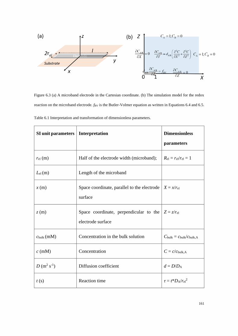
161
Figure 6.3 (a) A microband electrode in the Cartesian coordinate. (b) The simulation model for the redox
reaction on the microband electrode. fBV is the Butler-Volmer equation as written in Equations 6.4 and 6.5.
Table 6.1 Interpretation and transformation of dimensionless parameters.
SI unit parameters Interpretation Dimensionless
parameters
rel (m) Half of the electrode width (microband); Rel = rel/rel = 1
Lel (m) Length of the microband
x (m) Space coordinate, parallel to the electrode
surface
X = x/rel
z (m) Space coordinate, perpendicular to the
electrode surface
Z = z/rel
cbulk (mM) Concentration in the bulk solution Cbulk = cbulk/cbulk,A
c (mM) Concentration C = c/cbulk,A
D (m2 s-1) Diffusion coefficient d = D/DA
t (s) Reaction time τ = t*DA/rel2
162
SI unit parameters Interpretation Dimensionless
parameters
F (C mol-1) Faraday constant (96485 C mol-1)
R (J⋅mol−1⋅K−1) Gas constant (8.3145 J⋅mol−1⋅K−1)
T (K) Experiment temperature (298.2 K)
Ef (V) Formal potential
E (V) Applied electrode potential θ= (E - Ef)F/(RT)
k0 (m s-1) Standard electrochemical rate constant K = k0rel/DA
v (V s-1) Scan rate σ= vFrel2/(RTDA)
I (A) Current J = I/(FDAcbulk,ALel)
In this work, we focus on the single microband geometry, noting that although the current
at a microband electrode is often approximated to that of a hemicylinder of equivalent
area (𝑟 = 𝑤/𝜋, where 𝑟 is the radius of the hemicylinder and 𝑤 is the width of the band),
there is no true equivalence between these two geometries[4c]. In the following, we study
the true, not the approximate geometry.
6.3 Results and discussion
Voltammograms on a microband electrode were simulated for the cases of both fully
reversible and fully irreversible processes. We first aim to assess whether it is possible to
electrochemically measure the unknown width and length of a band electrode using an

163
electroactive redox couple. Second, we explore how the redox couple can be used to
characterise the band electrode with the minimum number of parameters known about the
selected redox couple. The results presented here focus exclusively on oxidative
voltammetry, but they are also equally applicable to reductive processes.
Unlike spherical or microdisc electrodes, a true steady state is impossible to obtain on
band electrodes under diffusion-controlled conditions because the mass transport operates
in two dimensions, one microscopic (the width) and one macroscopic (the length). This
situation leads to a quasi-steady state regime[4c, 7e, 12b]; single microband electrodes exhibit
quasi-steady state limiting currents at high overpotentials. The diffusional character
becomes more ‘linear’ for a wider band electrode of a given length (l), resulting in an
increasingly peaked waveshape. The magnitude of the current scales linearly with the
length of the band. It is the variability of waveshape which gives the possibility of the
measurement of width and length of a given band electrode from purely voltammetric
measurements, as will be shown below.
6.3.1 Fully reversible redox couple with equal diffusion coefficients
Reaction (6.1) was first simulated as a fully reversible electron transfer process at a
microband electrode where species A and B have equal diffusion coefficients.
Voltammograms simulated for electrodes with variable band widths are shown in Figure
6.4(a). The voltammograms normalised to the peak current are shown in Figure 6.4(b) in
order to compare the waveshapes. The diffusion coefficient used in the simulation is 7.81

164
× 10-10 m2 s-1 which is the value of the diffusion coefficient of species in the
ferrocenemethanol/ferrocenium methanol (FcCH2OH/FcCH2OH+) redox couple.[34] As
shown in Figure 6.4, although the waveshape becomes more peaked with wider bands,
for a reversible process, the changes in the waveshape are relatively subtle. Consequently,
the forward and backward peak potentials are too insensitive to the electrode dimensions
to be a useful measurement technique. Hence in this work, for characterising the electrode
dimensions, a reversible redox couple is not optimal for measuring the width and length
of a band electrode. The following section therefore focused on simulations for fully
irreversible processes where the redox couple has either equal or unequal diffusion
coefficients.
Figure 6.4 (a) Simulated voltammograms for a band electrode with variable widths for a fully reversible
process. (b) Normalised voltammograms of (a). The parameters in the simulation: scan rate ν = 0.2 V s-1,
diffusion coefficient D = 7.81 × 10⁻¹⁰ m2 s-1, formal potential Ef = 0 V, length of the band l = 1 × 10⁻² m,
electron transfer rate constant k0 = 1 m s-1, transfer coefficients αa = αc = 0.5.
-0.4 -0.2 0.0 0.2 0.4-0.2
-0.1
0.0
0.1
0.2
0.3
0.4
0.5
CVs on band electrode for a reversible process
Cu
rre
nt
/
A
Potential / V
w=100nm
w=200nm
w=400nm
w=800nm
w=1600nm
(a)
-0.4 -0.2 0.0 0.2 0.4-0.4
-0.2
0.0
0.2
0.4
0.6
0.8
1.0
Normalised CVs on band electrode for a reversible process
06/11/2018-2.1
I/I p
ea
k
Potential / V
w=100nm
w=200nm
w=400nm
w=800nm
w=1600nm
(b)
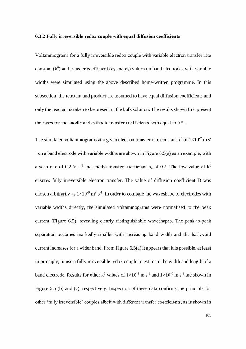
165
6.3.2 Fully irreversible redox couple with equal diffusion coefficients
Voltammograms for a fully irreversible redox couple with variable electron transfer rate
constant (k0) and transfer coefficient (αa and αc) values on band electrodes with variable
widths were simulated using the above described home-written programme. In this
subsection, the reactant and product are assumed to have equal diffusion coefficients and
only the reactant is taken to be present in the bulk solution. The results shown first present
the cases for the anodic and cathodic transfer coefficients both equal to 0.5.
The simulated voltammograms at a given electron transfer rate constant k0 of 1×10⁻⁷ m s-
1 on a band electrode with variable widths are shown in Figure 6.5(a) as an example, with
a scan rate of 0.2 V s-1 and anodic transfer coefficient αa of 0.5. The low value of k0
ensures fully irreversible electron transfer. The value of diffusion coefficient D was
chosen arbitrarily as 1×10⁻⁹ m2 s-1. In order to compare the waveshape of electrodes with
variable widths directly, the simulated voltammograms were normalised to the peak
current (Figure 6.5), revealing clearly distinguishable waveshapes. The peak-to-peak
separation becomes markedly smaller with increasing band width and the backward
current increases for a wider band. From Figure 6.5(a) it appears that it is possible, at least
in principle, to use a fully irreversible redox couple to estimate the width and length of a
band electrode. Results for other k0 values of 1×10⁻⁸ m s-1 and 1×10⁻⁹ m s-1 are shown in
Figure 6.5 (b) and (c), respectively. Inspection of these data confirms the principle for
other ‘fully irreversible’ couples albeit with different transfer coefficients, as is shown in
166
Figure 6.6 (αa= 0.3), Figure 6.7 (αa = 0.4), Figure 6.8 (αa = 0.6) and Figure 6.9 (αa = 0.7).
Figure 6.5 Normalised voltammograms for a band electrode with variable widths for a fully irreversible
redox couple with equal diffusion coefficients with various k0 of (a) 1×10⁻⁷, (b) 1×10⁻⁸ and (c) 1×10⁻⁹ m s-
1. The diffusion coefficients D(A)= D(B)=1×10⁻⁹ m2 s-1. Parameters in all simulations: ν=0.2 V s-1, Ef=0 V,
l=1×10⁻² m, transfer coefficients αa = αc = 0.5.
-1.0 -0.5 0.0 0.5 1.0 1.5-0.2
0.0
0.2
0.4
0.6
0.8
1.0
I/I p
ea
k
Potential / V
w=100nm
w=200nm
w=400nm
w=800nm
w=1600nm
(a)
D(A)=D(B)
-1.0 -0.5 0.0 0.5 1.0 1.5-0.2
0.0
0.2
0.4
0.6
0.8
1.0
I/I p
ea
k
Potential / V
w=100nm
w=200nm
w=400nm
w=800nm
w=1600nm
(b)
-1.0 -0.5 0.0 0.5 1.0 1.5-0.2
0.0
0.2
0.4
0.6
0.8
1.0
I/I p
ea
k
Potential / V
w=100nm
w=200nm
w=400nm
w=800nm
w=1600nm
(c)

167
Figure 6.6 Normalised voltammograms for a band electrode with variable widths for a fully irreversible
redox couple with equal diffusion coefficients with various k0 of (a) 1×10⁻⁷, (b) 1×10⁻⁸ and (c) 1×10⁻⁹ m s-
1. The diffusion coefficients D(A)= D(B)=1×10⁻⁹ m2 s-1. Parameters in all simulations: ν=0.2 V s-1, Ef=0 V,
l=1×10⁻² m, transfer coefficients αa = 0.3, αc = 0.7.
-1.0 -0.5 0.0 0.5 1.0 1.5
-0.2
0.0
0.2
0.4
0.6
0.8
1.0 Scan rate: 200 mV s-1
D=1.010-10 m2 s-1
k=1-9 m s-1
Ef=0 V
=0.7, =0.3
length=110-2 m
I/I p
ea
k
Potential / V
w=100 nm
w=200 nm
w=400 nm
w=800 nm
w=1600 nm
(c)
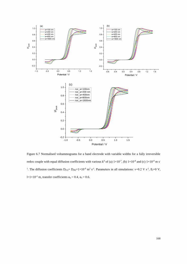
168
Figure 6.7 Normalised voltammograms for a band electrode with variable widths for a fully irreversible
redox couple with equal diffusion coefficients with various k0 of (a) 1×10⁻⁷, (b) 1×10⁻⁸ and (c) 1×10⁻⁹ m s-
1. The diffusion coefficients D(A)= D(B)=1×10⁻⁹ m2 s-1. Parameters in all simulations: ν=0.2 V s-1, Ef=0 V,
l=1×10⁻² m, transfer coefficients αa = 0.4, αc = 0.6.
-1.0 -0.5 0.0 0.5 1.0 1.5
-0.2
0.0
0.2
0.4
0.6
0.8
1.0 Scan rate: 200 mV s-1
D=1.010-10 m2 s-1
k=1-9 m s-1
Ef=0 V
=0.6, =0.4
length=110-2 m
I/I p
ea
k
Potential / V
nor_w=100nm
nor_w=200 nm
nor_w=400nm
nor_w=800nm
nor_w=1600nm
(c)
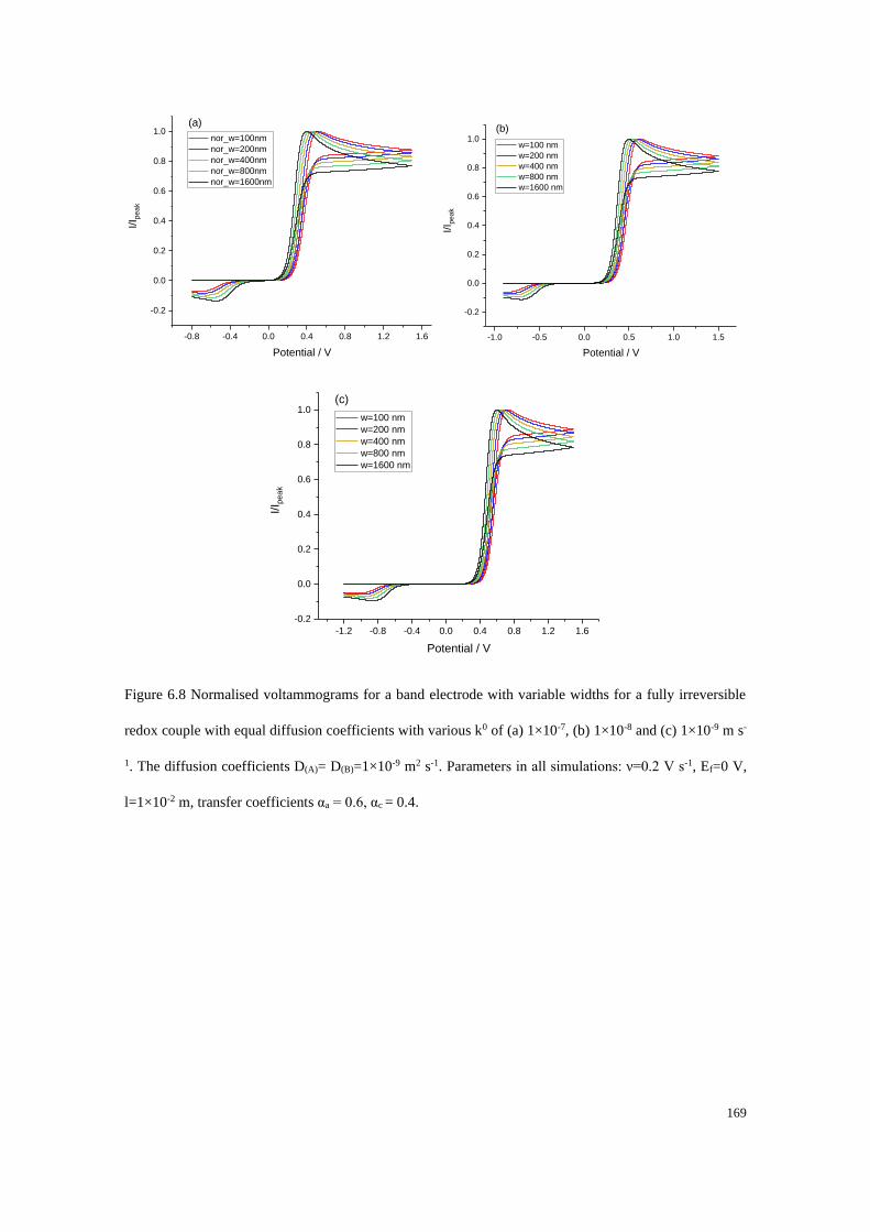
169
Figure 6.8 Normalised voltammograms for a band electrode with variable widths for a fully irreversible
redox couple with equal diffusion coefficients with various k0 of (a) 1×10⁻⁷, (b) 1×10⁻⁸ and (c) 1×10⁻⁹ m s-
1. The diffusion coefficients D(A)= D(B)=1×10⁻⁹ m2 s-1. Parameters in all simulations: ν=0.2 V s-1, Ef=0 V,
l=1×10⁻² m, transfer coefficients αa = 0.6, αc = 0.4.
-0.8 -0.4 0.0 0.4 0.8 1.2 1.6
-0.2
0.0
0.2
0.4
0.6
0.8
1.0 Scan rate: 200 mV s-1
D=1.010-10 m2 s-1
k=1-7 m s-1
Ef=0 V
=0.4, =0.6
length=110-2 m
I/I p
ea
k
Potential / V
nor_w=100nm
nor_w=200nm
nor_w=400nm
nor_w=800nm
nor_w=1600nm
(a)
-1.0 -0.5 0.0 0.5 1.0 1.5
-0.2
0.0
0.2
0.4
0.6
0.8
1.0Scan rate: 200 mV s-1
D=1.010-10 m2 s-1
k=1-8 m s-1
Ef=0 V
=0.4, =0.6
length=110-2 m
I/I p
ea
k
Potential / V
w=100 nm
w=200 nm
w=400 nm
w=800 nm
w=1600 nm
(b)
-1.2 -0.8 -0.4 0.0 0.4 0.8 1.2 1.6
-0.2
0.0
0.2
0.4
0.6
0.8
1.0Scan rate: 200 mV s-1
D=1.010-10 m2 s-1
k=1-9 m s-1
Ef=0 V
=0.4, =0.6
length=110-2 m
I/I p
ea
k
Potential / V
w=100 nm
w=200 nm
w=400 nm
w=800 nm
w=1600 nm
(c)
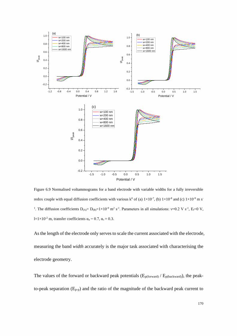
170
Figure 6.9 Normalised voltammograms for a band electrode with variable widths for a fully irreversible
redox couple with equal diffusion coefficients with various k0 of (a) 1×10⁻⁷, (b) 1×10⁻⁸ and (c) 1×10⁻⁹ m s-
1. The diffusion coefficients D(A)= D(B)=1×10⁻⁹ m2 s-1. Parameters in all simulations: ν=0.2 V s-1, Ef=0 V,
l=1×10⁻² m, transfer coefficients αa = 0.7, αc = 0.3.
As the length of the electrode only serves to scale the current associated with the electrode,
measuring the band width accurately is the major task associated with characterising the
electrode geometry.
The values of the forward or backward peak potentials (Ep(forward) / Ep(backward)), the peak-
to-peak separation (Ep-p) and the ratio of the magnitude of the backward peak current to
-1.2 -0.8 -0.4 0.0 0.4 0.8 1.2 1.6
-0.2
0.0
0.2
0.4
0.6
0.8
1.0
CVs on band electrode for an fully irreversible process
Scan rate: 200 mV s-1
D=1.010-10 m2 s-1
k=1-7 m s-1
Ef=0 V
=0.3, =0.7
length=110-2 m
I/I p
ea
k
Potential / V
w=100 nm
w=200 nm
w=400 nm
w=800 nm
w=1600 nm
(a)
-1.5 -1.0 -0.5 0.0 0.5 1.0 1.5
-0.2
0.0
0.2
0.4
0.6
0.8
1.0
Scan rate: 200 mV s-1
D=1.010-10 m2 s-1
k=1-8 m s-1
Ef=0 V
=0.3, =0.7
length=110-2 m
I/I p
ea
k
Potential / V
w=100 nm
w=200 nm
w=400 nm
w=800 nm
w=1600 nm
(b)
-1.5 -1.0 -0.5 0.0 0.5 1.0 1.5
-0.2
0.0
0.2
0.4
0.6
0.8
1.0Scan rate: 200 mV s-1
D=1.010-10 m2 s-1
k=1-9 m s-1
Ef=0 V
=0.3, =0.7
length=110-2 m
I/I p
ea
k
Potential / V
w=100 nm
w=200 nm
w=400 nm
w=800 nm
w=1600 nm
(c)
171
the forward peak current (|Ib/If|) are easily measured from an experimental voltammogram
and can be used to characterise and quantify the waveshape. Consequently, plots
describing Ep(forward) or Ep(backward), Ep-p and |Ib/If| as a function of band width were
considered as the diagnostic parameters via which the measurement of band width and
length may be made. Since the transfer coefficient αa and diffusion coefficient D can be
relatively easily measured from experiments, the remaining unknown parameters are the
formal potential Ef and electron transfer rate constant k0. The next step in this work is to
reduce the number of parameters needed for the characterisation of the geometry of band
electrodes.
Considering that the use of peak potential as a diagnostic would require knowledge of the
formal potential, the peak-to-peak separation was used instead. Voltammograms on a
band electrode with variable k0 were simulated, at a scan rate of 0.2 V s-1, anodic transfer
coefficient αa of 0.5 and diffusion coefficient D of 1×10⁻⁹ m2 s-1. The corresponding plots
of the two different diagnostic parameters, Ep-p and |Ib/If|, as a function of band width are
shown in Figure 6.10. According to Figure 6.10, with a known peak to peak separation
(Ep-p) or ratio of the magnitude of backward peak current to forward peak current (|Ib/If|),
an accurate measurement of k0 is needed to avoid a large error in the estimation of width.
Consequently, the combination of plots of both Ep-p and |Ib/If| with variable band widths
were chosen as the basis for the sought discrimination. For any given band electrode, the
band width estimated from the plot of Ep-p versus band width must be consistent with that
from the plot of |Ib/If| versus band width. In this way, by combining the measurements of

172
Ep-p and |Ib/If|, the band width can be estimated without the knowledge of formal potential
Ef and electron transfer rate constant k0. This facilitates the measurement of the band
width without any prior knowledge of k0. The parameters required for the measurement
of band width using different analysing indicators are tabulated in Table 6.2.
Figure 6.10 (a) Plot of Ep-p as a function of band widths with variable k0. (b) Plot of |Ibackward/Iforward| as a
function of band widths with variable k0. Parameters in the simulations: αa = αc = 0.5, D(A) = D(B) = 1×10⁻⁹
m2 s-1. The dotted line shows the corresponding band width at different k0.
Table 6.2 Parameters required for the measurement of band width and length using different indicators.
Indications Ep(forward) vs Ef Ep-p |Ibackward/Iforward| Ep-p and |Ibackward/Iforward|
Parameters
required
αa αa αa αa
D D D D
k0 k0 k0
Ef
0 200 400 600 800 1000 1200 1400 1600 1800
1.2
1.4
1.6
1.8
2.0
Ep-p
/ V
Band width / nm
k=110-9 m s-1
k=110-8 m s-1
k=110-7 m s-1
(a)
0 200 400 600 800 1000 1200 1400 1600 1800
0.04
0.05
0.06
0.07
0.08
0.09
0.10
I b
ackw
ard
/Ifo
rwa
rd
Band width / nm
k=110-9 m s-1
k=110-8 m s-1
k=110-7 m s-1
(b)
173
6.3.3 Fully irreversible redox couple with unequal diffusion coefficients
Considering that the electroactive redox species might have different diffusion
coefficients for the oxidised and reduced species, reaction (6.1) was also simulated on a
band electrode for the case where species A and B have unequal diffusion coefficients
but again only, with the reactant (A) initially present in bulk solution. Again the results
shown first assume that the anodic and cathodic transfer coefficients equal 0.5. Results
for other transfer coefficients are shown in Figure 6.12 (αa= 0.3), Figure 6.13 (αa = 0.4),
Figure 6.14 (αa = 0.6) and Figure 6.15 (αa = 0.7), with similar conclusions drawn as to
those below.
The simulated and normalised voltammograms at the various given electron transfer rate
constants (k0 = 1×10⁻⁷, 1×10⁻⁸ and 1×10⁻⁹ m s-1) on a band electrode with variable band
widths are shown in Figure 6.11(a), (b) and (c), respectively, with a scan rate of 0.2 V s-
1, anodic transfer coefficient αa of 0.5, diffusion coefficient D(A) of 1×10⁻⁹ m2 s-1 and
diffusion coefficient D(B) of 5×10⁻¹⁰ m2 s-1. The comparison of waveshape was achieved
through the normalisation of the voltammogram relative to the peak current.
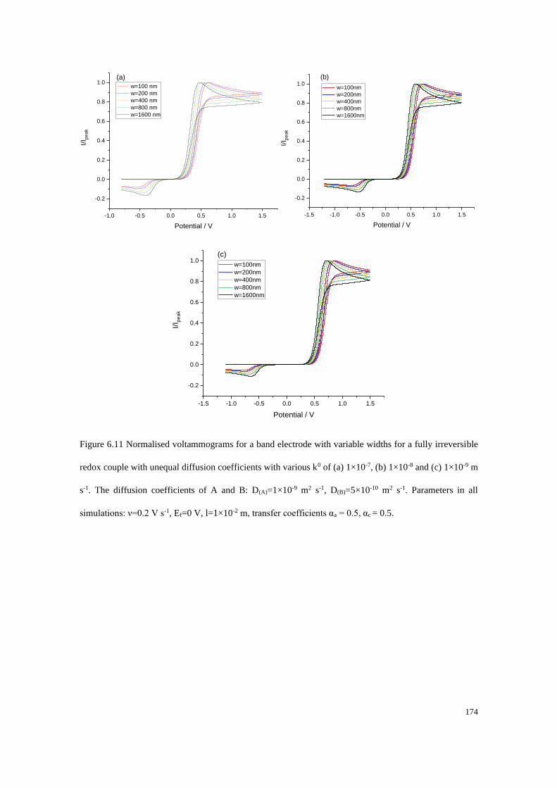
174
Figure 6.11 Normalised voltammograms for a band electrode with variable widths for a fully irreversible
redox couple with unequal diffusion coefficients with various k0 of (a) 1×10⁻⁷, (b) 1×10⁻⁸ and (c) 1×10⁻⁹ m
s-1. The diffusion coefficients of A and B: D(A)=1×10⁻⁹ m2 s-1, D(B)=5×10⁻¹⁰ m2 s-1. Parameters in all
simulations: ν=0.2 V s-1, Ef=0 V, l=1×10⁻² m, transfer coefficients αa = 0.5, αc = 0.5.
-1.0 -0.5 0.0 0.5 1.0 1.5
-0.2
0.0
0.2
0.4
0.6
0.8
1.0 Scan rate: 200 mV s-1
D(A)=1.010-10 m2 s-1
D(B)=0.510-10 m2 s-1
k=1-7 m s-1
Ef=0 V
=0.5, =0.5
length=110-2 m
I/I p
ea
k
Potential / V
w=100 nm
w=200 nm
w=400 nm
w=800 nm
w=1600 nm
(a)
-1.5 -1.0 -0.5 0.0 0.5 1.0 1.5
-0.2
0.0
0.2
0.4
0.6
0.8
1.0
I/I p
ea
k
Potential / V
w=100nm
w=200nm
w=400nm
w=800nm
w=1600nm
(b)
-1.5 -1.0 -0.5 0.0 0.5 1.0 1.5
-0.2
0.0
0.2
0.4
0.6
0.8
1.0
I/I p
ea
k
Potential / V
w=100nm
w=200nm
w=400nm
w=800nm
w=1600nm
(c)
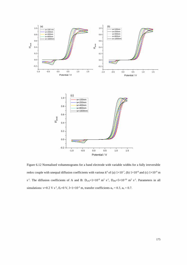
175
Figure 6.12 Normalised voltammograms for a band electrode with variable widths for a fully irreversible
redox couple with unequal diffusion coefficients with various k0 of (a) 1×10⁻⁷, (b) 1×10⁻⁸ and (c) 1×10⁻⁹ m
s-1. The diffusion coefficients of A and B: D(A)=1×10⁻⁹ m2 s-1, D(B)=5×10⁻¹⁰ m2 s-1. Parameters in all
simulations: ν=0.2 V s-1, Ef=0 V, l=1×10⁻² m, transfer coefficients αa = 0.3, αc = 0.7.
-1.0 -0.5 0.0 0.5 1.0 1.5
-0.2
0.0
0.2
0.4
0.6
0.8
1.0I/I p
ea
k
Potential / V
w=100 nm
w=200nm
w=400nm
w=800nm
w=1600nm
(a)k-1e-7
b=0.3
-1.0 -0.5 0.0 0.5 1.0 1.5
-0.2
0.0
0.2
0.4
0.6
0.8
1.0
I/I p
ea
k
Potential / V
w=100nm
w=200nm
w=400nm
w=800nm
w=1600nm
(b)
-1.0 -0.5 0.0 0.5 1.0 1.5
-0.2
0.0
0.2
0.4
0.6
0.8
1.0
I/I p
ea
k
Potential / V
w=100nm
w=200nm
w=400nm
w=800nm
w=1600nm
(c)

176
Figure 6.13 Normalised voltammograms for a band electrode with variable widths for a fully irreversible
redox couple with unequal diffusion coefficients with various k0 of (a) 1×10⁻⁷, (b) 1×10⁻⁸ and (c) 1×10⁻⁹ m
s-1. The diffusion coefficients of A and B: D(A)=1×10⁻⁹ m2 s-1, D(B)=5×10⁻¹⁰ m2 s-1. Parameters in all
simulations: ν=0.2 V s-1, Ef=0 V, l=1×10⁻² m, transfer coefficients αa = 0.4, αc = 0.6.
-1.0 -0.5 0.0 0.5 1.0 1.5
-0.2
0.0
0.2
0.4
0.6
0.8
1.0I/I p
ea
k
Potential / V
w=100 nm
w=200nm
w=400nm
w=800nm
w=1600nm
(a)
-1.0 -0.5 0.0 0.5 1.0 1.5
-0.2
0.0
0.2
0.4
0.6
0.8
1.0
I/I p
ea
k
Potential / V
w=100nm
w=200nm
w=400nm
w=800nm
w=1600nm
(b)
-1.0 -0.5 0.0 0.5 1.0 1.5
-0.2
0.0
0.2
0.4
0.6
0.8
1.0
I/I p
ea
k
Potential / V
w=100nm
w=200nm
w=400nm
w=800nm
w=1600nm
(c)
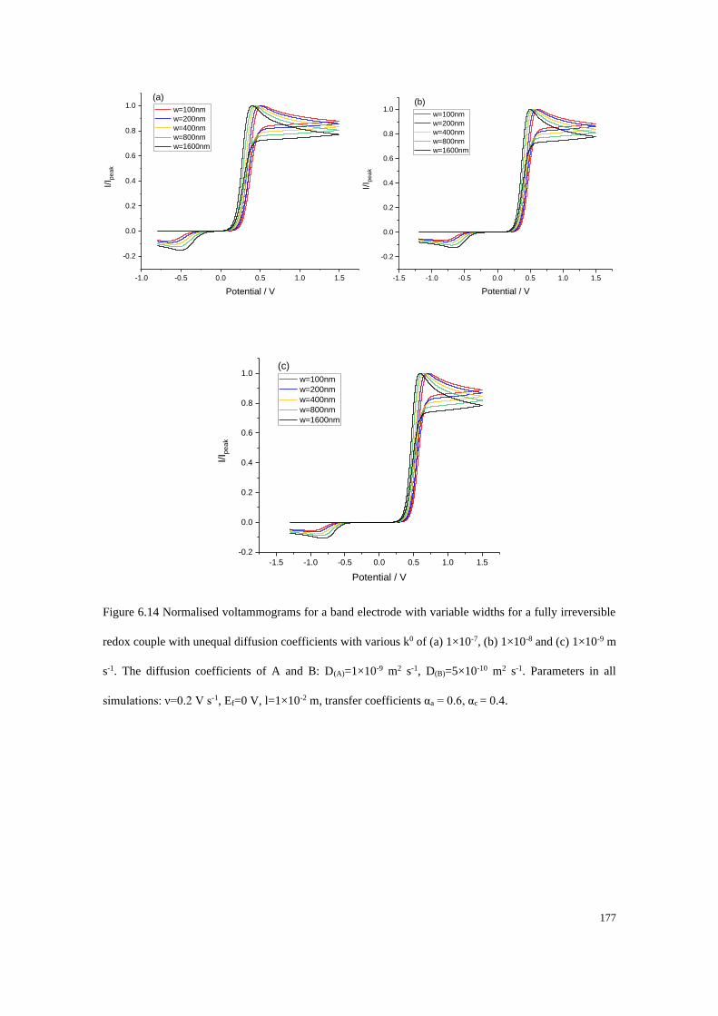
177
Figure 6.14 Normalised voltammograms for a band electrode with variable widths for a fully irreversible
redox couple with unequal diffusion coefficients with various k0 of (a) 1×10⁻⁷, (b) 1×10⁻⁸ and (c) 1×10⁻⁹ m
s-1. The diffusion coefficients of A and B: D(A)=1×10⁻⁹ m2 s-1, D(B)=5×10⁻¹⁰ m2 s-1. Parameters in all
simulations: ν=0.2 V s-1, Ef=0 V, l=1×10⁻² m, transfer coefficients αa = 0.6, αc = 0.4.
-1.0 -0.5 0.0 0.5 1.0 1.5
-0.2
0.0
0.2
0.4
0.6
0.8
1.0I/I p
ea
k
Potential / V
w=100nm
w=200nm
w=400nm
w=800nm
w=1600nm
(a)
-1.5 -1.0 -0.5 0.0 0.5 1.0 1.5
-0.2
0.0
0.2
0.4
0.6
0.8
1.0
I/I p
ea
k
Potential / V
w=100nm
w=200nm
w=400nm
w=800nm
w=1600nm
(b)
-1.5 -1.0 -0.5 0.0 0.5 1.0 1.5
-0.2
0.0
0.2
0.4
0.6
0.8
1.0
I/I p
ea
k
Potential / V
w=100nm
w=200nm
w=400nm
w=800nm
w=1600nm
(c)
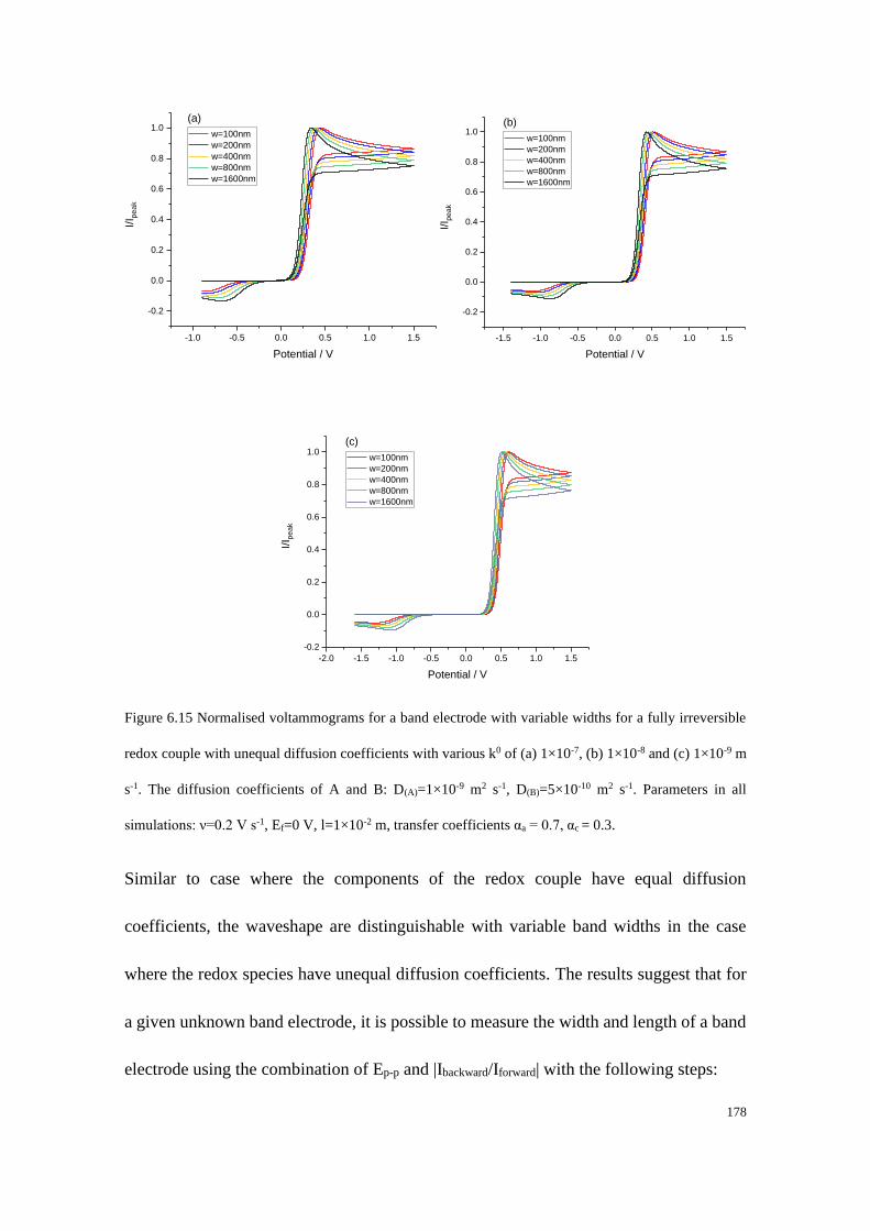
178
Figure 6.15 Normalised voltammograms for a band electrode with variable widths for a fully irreversible
redox couple with unequal diffusion coefficients with various k0 of (a) 1×10⁻⁷, (b) 1×10⁻⁸ and (c) 1×10⁻⁹ m
s-1. The diffusion coefficients of A and B: D(A)=1×10⁻⁹ m2 s-1, D(B)=5×10⁻¹⁰ m2 s-1. Parameters in all
simulations: ν=0.2 V s-1, Ef=0 V, l=1×10⁻² m, transfer coefficients αa = 0.7, αc = 0.3.
Similar to case where the components of the redox couple have equal diffusion
coefficients, the waveshape are distinguishable with variable band widths in the case
where the redox species have unequal diffusion coefficients. The results suggest that for
a given unknown band electrode, it is possible to measure the width and length of a band
electrode using the combination of Ep-p and |Ibackward/Iforward| with the following steps:
-1.0 -0.5 0.0 0.5 1.0 1.5
-0.2
0.0
0.2
0.4
0.6
0.8
1.0I/I p
ea
k
Potential / V
w=100nm
w=200nm
w=400nm
w=800nm
w=1600nm
(a)
-1.5 -1.0 -0.5 0.0 0.5 1.0 1.5
-0.2
0.0
0.2
0.4
0.6
0.8
1.0
I/I p
ea
k
Potential / V
w=100nm
w=200nm
w=400nm
w=800nm
w=1600nm
(b)
-2.0 -1.5 -1.0 -0.5 0.0 0.5 1.0 1.5
-0.2
0.0
0.2
0.4
0.6
0.8
1.0
I/I p
ea
k
Potential / V
w=100nm
w=200nm
w=400nm
w=800nm
w=1600nm
(c)
179
1. Determination of DA, DB, αa and αc: experimentally measure the diffusion
coefficients (DA and DB) of the redox species from the steady-state current obtained
on a microdisc electrode using double potential step chronoamperometry if
necessary to give both diffusion coefficients[35]. Calculate the transfer coefficient (αa)
using Tafel analysis from the experimental voltammogram for a one-electron
transfer oxidative process[33]. The cathodic transfer coefficient αc equals (1- αa) with
a common assumption that the transfer coefficients equal to unity; a more in-depth
discussion is presented in Chapter 5.
2. Determination of k0 and w: calculate the values of Ep-p and |Ibackward/Iforward| from the
experimental voltammogram. Using the simulations with a set of k0 and band widths
and the corresponding plots of Ep-p versus band width and |Ibackward/Iforward| versus
band width. By comparing the experimental and theoretical values of Ep-p and
|Ibackward/Iforward|, k0 and band width can be estimated (the values of k0 and w are
unique for a given experimental voltammogram on a band electrode).
3. Determination of band length: by modelling a simulation with the measured transfer
coefficient and diffusion coefficients along with the estimated k0 and w, the length
of the band can be calculated using Equation 6.8.
𝑙𝑒𝑛𝑔𝑡ℎ =𝐸𝑥𝑝𝑒𝑟𝑖𝑚𝑒𝑛𝑡𝑎𝑙 𝐼𝑝𝑒𝑎𝑘 (𝜇𝐴)
𝑆𝑖𝑚𝑢𝑙𝑎𝑡𝑒𝑑 𝐼𝑝𝑒𝑎𝑘
𝑙𝑒𝑛𝑔𝑡ℎ (𝜇𝐴 𝑚−1)
(6.8)
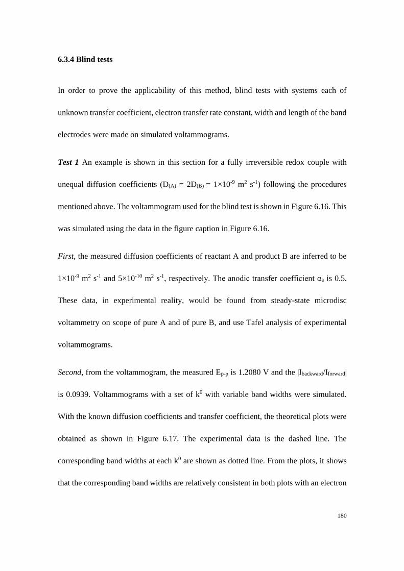
180
6.3.4 Blind tests
In order to prove the applicability of this method, blind tests with systems each of
unknown transfer coefficient, electron transfer rate constant, width and length of the band
electrodes were made on simulated voltammograms.
Test 1 An example is shown in this section for a fully irreversible redox couple with
unequal diffusion coefficients (D(A) = 2D(B) = 1×10⁻⁹ m2 s-1) following the procedures
mentioned above. The voltammogram used for the blind test is shown in Figure 6.16. This
was simulated using the data in the figure caption in Figure 6.16.
First, the measured diffusion coefficients of reactant A and product B are inferred to be
1×10⁻⁹ m2 s-1 and 5×10⁻¹⁰ m2 s-1, respectively. The anodic transfer coefficient αa is 0.5.
These data, in experimental reality, would be found from steady-state microdisc
voltammetry on scope of pure A and of pure B, and use Tafel analysis of experimental
voltammograms.
Second, from the voltammogram, the measured Ep-p is 1.2080 V and the |Ibackward/Iforward|
is 0.0939. Voltammograms with a set of k0 with variable band widths were simulated.
With the known diffusion coefficients and transfer coefficient, the theoretical plots were
obtained as shown in Figure 6.17. The experimental data is the dashed line. The
corresponding band widths at each k0 are shown as dotted line. From the plots, it shows
that the corresponding band widths are relatively consistent in both plots with an electron

181
transfer rate constant k0 of 7.5×10⁻⁸ m s-1. The band width was therefore estimated as
1056 nm.
Third, further simulation was done with the known transfer coefficient of 0.5, diffusion
coefficients of reactant and product of 1×10⁻⁹ m2 s-1 and 5×10⁻¹⁰ m2 s-1, estimated rate
constant of 7.5×10⁻⁸ m s-1 and band width of 1056 nm. The corresponding voltammogram
was normalised to its length as shown in Figure 6.18. The length of the band in the blind
test was then calculated using Equation 6.8 and was 0.0180 m. Therefore, the band width
was estimated as 1056 nm with a length of 0.0180 m (the true width is 1058 nm and the
true length is 0.018 m). The errors are 0.19% and 0.034% in width and length,
respectively as shown in Table 6.3 ‘Test 1’.
𝑙𝑒𝑛𝑔𝑡ℎ =𝐸𝑥𝑝𝑒𝑟𝑖𝑚𝑒𝑛𝑡𝑎𝑙 𝐼𝑝𝑒𝑎𝑘 (𝜇𝐴)
𝑆𝑖𝑚𝑢𝑙𝑎𝑡𝑒𝑑 𝐼𝑝𝑒𝑎𝑘
𝑙𝑒𝑛𝑔𝑡ℎ (𝜇𝐴 𝑚−1)
=1.0192 𝜇𝐴
56.6030 𝜇𝐴 𝑚−1 = 0.0180 𝑚

182
Figure 6.16 Blind test on a band electrode with unknown band length and width. Known parameters in the
simulation: c = 1 mM, ν = 0.2 V s-1, αa = αc = 0.5, D(A) = 1×10⁻⁹ m2 s-1, D(B) = 5×10⁻¹⁰ m2 s-1.
Figure 6.17 (a) Plot of Ep-p as a function of band widths with variable k0. (b) Plot of |Ibackward/Iforward|as a
function of band widths with variable k0. Parameters in the simulations: αa = αc = 0.5, D(A) = 1×10⁻⁹ m2 s-1,
D(B) = 5×10⁻¹⁰ m2 s-1. The dashed line is the measured value of Ep-p and |Ibackward/Iforward| from Figure 6.16.
The dotted line shows the corresponding band width at different k0.
-1.0 -0.5 0.0 0.5 1.0 1.5-0.2
0.0
0.2
0.4
0.6
0.8
1.0
1.2
Curr
ent /
A
Potential vs SCE / V
Test 1
0 200 400 600 800 1000 1200 1400 1600 18001.10
1.15
1.20
1.25
1.30
1.35
1.40
1.45
1.50
Ep-p
/ V
Band width / nm
k=510-8 m s-1
k=7.510-8 m s-1
k=110-7 m s-1
Test 4
(a)
0 200 400 600 800 1000 1200 1400 1600 18000.05
0.06
0.07
0.08
0.09
0.10
0.11
I b
ackw
ard
/Ifo
rwa
rd
Band width / nm
k=510-8 m s-1,
k=7.510-8 m s-1
k=110-7 m s-1
Test 4
(b)
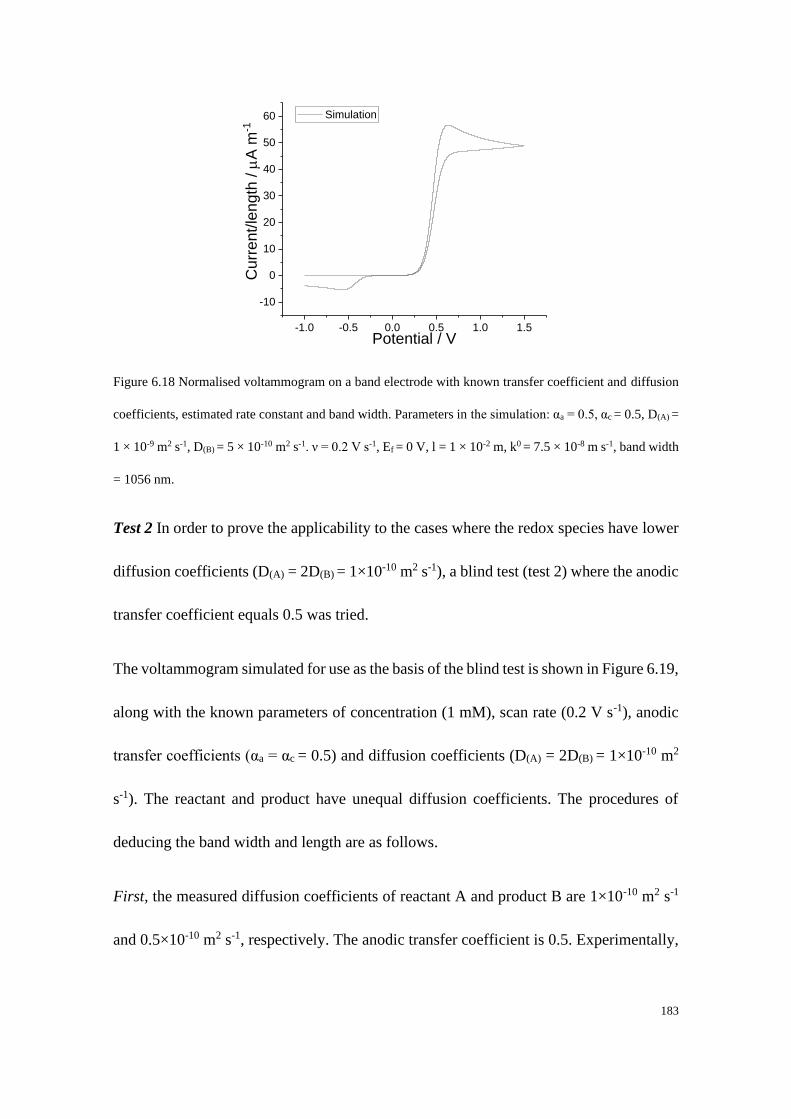
183
Figure 6.18 Normalised voltammogram on a band electrode with known transfer coefficient and diffusion
coefficients, estimated rate constant and band width. Parameters in the simulation: αa = 0.5, αc = 0.5, D(A) =
1 × 10⁻⁹ m2 s-1, D(B) = 5 × 10⁻¹⁰ m2 s-1. ν = 0.2 V s-1, Ef = 0 V, l = 1 × 10⁻² m, k0 = 7.5 × 10⁻⁸ m s-1, band width
= 1056 nm.
Test 2 In order to prove the applicability to the cases where the redox species have lower
diffusion coefficients (D(A) = 2D(B) = 1×10⁻¹⁰ m2 s-1), a blind test (test 2) where the anodic
transfer coefficient equals 0.5 was tried.
The voltammogram simulated for use as the basis of the blind test is shown in Figure 6.19,
along with the known parameters of concentration (1 mM), scan rate (0.2 V s-1), anodic
transfer coefficients (αa = αc = 0.5) and diffusion coefficients (D(A) = 2D(B) = 1×10⁻¹⁰ m2
s-1). The reactant and product have unequal diffusion coefficients. The procedures of
deducing the band width and length are as follows.
First, the measured diffusion coefficients of reactant A and product B are 1×10⁻¹⁰ m2 s-1
and 0.5×10⁻¹⁰ m2 s-1, respectively. The anodic transfer coefficient is 0.5. Experimentally,
-1.0 -0.5 0.0 0.5 1.0 1.5
-10
0
10
20
30
40
50
60
Curr
ent/le
ngth
/
A m
-1
Potential / V
Simulation
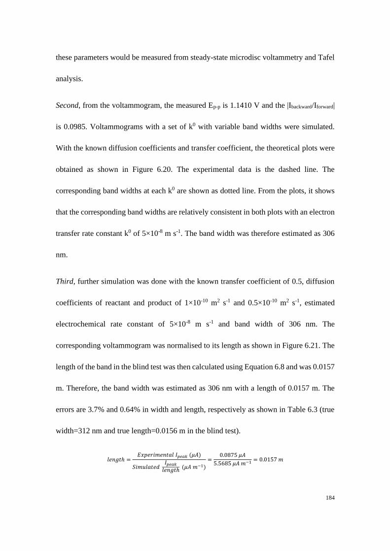
184
these parameters would be measured from steady-state microdisc voltammetry and Tafel
analysis.
Second, from the voltammogram, the measured Ep-p is 1.1410 V and the |Ibackward/Iforward|
is 0.0985. Voltammograms with a set of k0 with variable band widths were simulated.
With the known diffusion coefficients and transfer coefficient, the theoretical plots were
obtained as shown in Figure 6.20. The experimental data is the dashed line. The
corresponding band widths at each k0 are shown as dotted line. From the plots, it shows
that the corresponding band widths are relatively consistent in both plots with an electron
transfer rate constant k0 of 5×10⁻⁸ m s-1. The band width was therefore estimated as 306
nm.
Third, further simulation was done with the known transfer coefficient of 0.5, diffusion
coefficients of reactant and product of 1×10⁻¹⁰ m2 s-1 and 0.5×10⁻¹⁰ m2 s-1, estimated
electrochemical rate constant of 5×10⁻⁸ m s-1 and band width of 306 nm. The
corresponding voltammogram was normalised to its length as shown in Figure 6.21. The
length of the band in the blind test was then calculated using Equation 6.8 and was 0.0157
m. Therefore, the band width was estimated as 306 nm with a length of 0.0157 m. The
errors are 3.7% and 0.64% in width and length, respectively as shown in Table 6.3 (true
width=312 nm and true length=0.0156 m in the blind test).
𝑙𝑒𝑛𝑔𝑡ℎ =𝐸𝑥𝑝𝑒𝑟𝑖𝑚𝑒𝑛𝑡𝑎𝑙 𝐼𝑝𝑒𝑎𝑘 (𝜇𝐴)
𝑆𝑖𝑚𝑢𝑙𝑎𝑡𝑒𝑑 𝐼𝑝𝑒𝑎𝑘
𝑙𝑒𝑛𝑔𝑡ℎ (𝜇𝐴 𝑚−1)
=0.0875 𝜇𝐴
5.5685 𝜇𝐴 𝑚−1 = 0.0157 𝑚
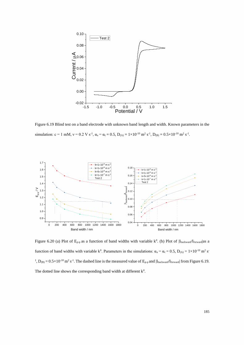
185
Figure 6.19 Blind test on a band electrode with unknown band length and width. Known parameters in the
simulation: c = 1 mM, ν = 0.2 V s-1, αa = αc = 0.5, D(A) = 1×10⁻¹⁰ m2 s-1, D(B) = 0.5×10⁻¹⁰ m2 s-1.
Figure 6.20 (a) Plot of Ep-p as a function of band widths with variable k0. (b) Plot of |Ibackward/Iforward|as a
function of band widths with variable k0. Parameters in the simulations: αa = αc = 0.5, D(A) = 1×10⁻¹⁰ m2 s-
1, D(B) = 0.5×10⁻¹⁰ m2 s-1. The dashed line is the measured value of Ep-p and |Ibackward/Iforward| from Figure 6.19.
The dotted line shows the corresponding band width at different k0.
-1.5 -1.0 -0.5 0.0 0.5 1.0 1.5-0.02
0.00
0.02
0.04
0.06
0.08
0.10
Curr
ent /
A
Potential / V
Test 2
0 200 400 600 800 1000 1200 1400 1600 1800
0.9
1.0
1.1
1.2
1.3
1.4
1.5
1.6
1.7
Ep
-p / V
Band width / nm
k=110-9 m s-1
k=110-8 m s-1
k=510-8 m s-1
k=110-7 m s-1
Test 2
0 200 400 600 800 1000 1200 1400 1600 1800
0.04
0.06
0.08
0.10
0.12
0.14
0.16
0.18
Ib
ackw
ard
/Ifo
rwa
rd
Band width / nm
k=110-9 m s-1
k=110-8 m s-1
k=510-8 m s-1
k=110-7 m s-1
Test 2
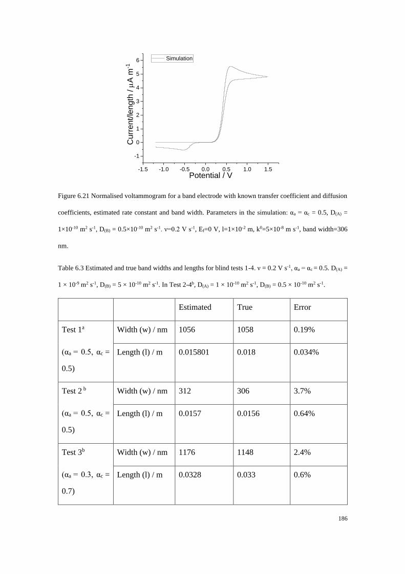
186
Figure 6.21 Normalised voltammogram for a band electrode with known transfer coefficient and diffusion
coefficients, estimated rate constant and band width. Parameters in the simulation: αa = αc = 0.5, D(A) =
1×10⁻¹⁰ m2 s-1, D(B) = 0.5×10⁻¹⁰ m2 s-1. ν=0.2 V s-1, Ef=0 V, l=1×10⁻² m, k0=5×10⁻⁸ m s-1, band width=306
nm.
Table 6.3 Estimated and true band widths and lengths for blind tests 1-4. ν = 0.2 V s-1, αa = αc = 0.5. D(A) =
1 × 10⁻⁹ m2 s-1, D(B) = 5 × 10⁻¹⁰ m2 s-1. In Test 2-4b, D(A) = 1 × 10⁻¹⁰ m2 s-1, D(B) = 0.5 × 10⁻¹⁰ m2 s-1.
Estimated True Error
Test 1a
(αa = 0.5, αc =
0.5)
Width (w) / nm 1056 1058 0.19%
Length (l) / m 0.015801 0.018 0.034%
Test 2 b
(αa = 0.5, αc =
0.5)
Width (w) / nm 312 306 3.7%
Length (l) / m 0.0157 0.0156 0.64%
Test 3b
(αa = 0.3, αc =
0.7)
Width (w) / nm 1176 1148 2.4%
Length (l) / m 0.0328 0.033 0.6%
-1.5 -1.0 -0.5 0.0 0.5 1.0 1.5
-1
0
1
2
3
4
5
6
Curr
ent/le
ngth
/
A m
-1
Potential / V
Simulation

187
Test 4 b
(αa = 0.4, αc =
0.6)
Width (w) / nm 1424 1350 5.5%
Length (l) / m 0.0444 0.045 1.3%
The analysing details for other transfer coefficients are presented in the Appendix C2.
The estimated dimensions of the band electrodes are tabulated in Table 6.3. According to
the results in Table 6.3, it is shown that by using this method, in all cases the error in
width is 3.9% ± 1.6% and the error in length is 0.85% ± 0.40%.
6.4 Conclusions
This work validates an entirely voltammetric method to characterise the dimensions of a
band electrode. With a given unknown band electrode, the band width and length can be
estimated electrochemically by using a fully irreversible redox couple without any prior
knowledge of electron transfer rate constant k0 and/or the formal potential Ef. Considering
that the diffusion coefficient of the electroactive species and the transfer coefficient can
be measured from experiments, the peak-to-peak separation Ep-p and the ratio of the
magnitude of backward peak current to forward peak current |Ibackward/Iforward| are
combined together as the indicators to estimate the electron transfer rate constant and the
band width. From the blind test, the estimated band width and length gave errors of ~4%
and ~1%, respectively.
188
References:
[1] D. Li, C. Lin, C. Batchelor-McAuley, L. Chen, R. G. Compton, Journal of Electroanalytical
Chemistry 2019, 840, 279-284.
[2] D. Li, C. Batchelor-McAuley, L. Chen, R. G. Compton, ACS Sens 2019, 4, 2250-2266.
[3] S. Karel, A. Christian, H. Karel, M. Vladimír, K. Wlodzimierz, Pure and Applied Chemistry 2000,
72, 1483-1492.
[4] aJ. Heinze, Angewandte Chemie International Edition in English 1993, 32, 1268-1288; bR. J.
Forster, Chemical Society Reviews 1994, 23, 289-297; cR. G. A. B. Compton, Craig E,
Understanding Voltammetry, third ed., World Scientific, 2018.
[5] K. R. Wehmeyer, M. R. Deakin, R. M. Wightman, Analytical Chemistry 1985, 57, 1913-1916.
[6] aI. A. Silver, I. Bergman, M. Akhtar, C. R. Lowe, I. J. Higgins, Philosophical Transactions of the
Royal Society of London. B, Biological Sciences 1987, 316, 161-167; bE. Llaudet, S. Hatz, M.
Droniou, N. Dale, Analytical Chemistry 2005, 77, 3267-3273.
[7] aJ. Fraden, Handbook of Modern Sensors: Physics, Designs, and Applications, Springer New York,
2010; bW. Qiu, M. Xu, R. Li, X. Liu, M. Zhang, Analytical Chemistry 2016, 88, 1117-1122; cK.
C. Honeychurch, S. Al-Berezanchi, J. P. Hart, Talanta 2011, 84, 717-723; dJ. P. Metters, R. O.
Kadara, C. E. Banks, Sensors and Actuators B: Chemical 2012, 169, 136-143; eC. Sapsanis, H.
Omran, V. Chernikova, O. Shekhah, Y. Belmabkhout, U. Buttner, M. Eddaoudi, K. N. Salama,
Sensors 2015, 15, 18153-18166.
[8] aR. M. Pemberton, J. Xu, R. Pittson, G. A. Drago, J. Griffiths, S. K. Jackson, J. P. Hart, Biosensors
and Bioelectronics 2011, 26, 2448-2453; bD. Sharma, Y. Lim, Y. Lee, H. Shin, Analytica Chimica
Acta 2015, 889, 194-202; cM. Falk, R. Sultana, M. J. Swann, A. R. Mount, N. J. Freeman,
Bioelectrochemistry 2016, 112, 100-105; dK. Dawson, M. Baudequin, A. O'Riordan, Analyst 2011,
136, 4507-4513.
[9] P. Mehrotra, Journal of Oral Biology and Craniofacial Research 2016, 6, 153-159.
[10] J. Wang, G. Chen, M. P. Chatrathi, A. Fujishima, D. A. Tryk, D. Shin, Analytical Chemistry 2003,
75, 935-939.
[11] L. Wang, M. Veselinovic, L. Yang, B. J. Geiss, D. S. Dandy, T. Chen, Biosensors and
Bioelectronics 2017, 87, 646-653.
[12] aA. M. Bond, M. Fleischmann, J. Robinson, Journal of Electroanalytical Chemistry and
Interfacial Electrochemistry 1984, 168, 299-312; bM. A. Hernández-Olmos, L. Agüı, P. Yáñez-
Sedeño, J. M. Pingarrón, Electrochimica Acta 2000, 46, 289-296.
[13] F. Zhang, M. A. Edwards, R. Hao, H. S. White, B. Zhang, The Journal of Physical Chemistry C
2017, 121, 23564-23573.
[14] X. Li, C. Batchelor-McAuley, L. Shao, S. V. Sokolov, N. P. Young, R. G. Compton, The Journal
of Physical Chemistry Letters 2017, 8, 507-511.
[15] R. B. Morris, D. J. Franta, H. S. White, The Journal of Physical Chemistry 1987, 91, 3559-3564.
[16] J.-L. Chang, J.-M. Zen, Electrochemistry Communications 2006, 8, 571-576.
[17] aY. H. Lanyon, D. W. M. Arrigan, Sensors and Actuators B: Chemical 2007, 121, 341-347; bC.
S. Henry, Journal of The Electrochemical Society 1999, 146, 3367.
189
[18] L. Angnes, E. M. Richter, M. A. Augelli, G. H. Kume, Analytical Chemistry 2000, 72, 5503-5506.
[19] aT. A. Postlethwaite, J. E. Hutchison, R. Murray, B. Fosset, C. Amatore, Analytical Chemistry
1996, 68, 2951-2958; bD. M. Odell, W. J. Bowyer, Analytical Chemistry 1990, 62, 1619-1623.
[20] P. M. Kovach, W. L. Caudill, D. G. Peters, R. M. Wightman, Journal of Electroanalytical
Chemistry and Interfacial Electrochemistry 1985, 185, 285-295.
[21] R. Lin, T. M. Lim, T. Tran, Electrochemistry Communications 2018, 86, 135-139.
[22] aD. H. Craston, C. P. Jones, D. E. Williams, N. El Murr, Talanta 1991, 38, 17-26; bD. E. Williams,
K. Ellis, A. Colville, S. J. Dennison, G. Laguillo, J. Larsen, Journal of Electroanalytical Chemistry
1997, 432, 159-169.
[23] aT. R. L. C. Paixão, R. C. Matos, M. Bertotti, Electroanalysis 2003, 15, 1884-1889; bH. A. O.
Hill, N. A. Klein, I. S. M. Psalti, N. J. Walton, Analytical Chemistry 1989, 61, 2200-2206; cJ. E.
Bartelt, M. R. Deakin, C. Amatore, R. M. Wightman, Analytical Chemistry 1988, 60, 2167-2169;
dT. V. Shea, A. J. Bard, Analytical Chemistry 1987, 59, 2101-2111.
[24] aN. Creedon, R. Sayers, B. O'Sullivan, e. kennedy, P. Lovera, A. O'Riordan, Label-Free
Impedimetric Nanoband Sensor for Detection of Both Bovine Viral Diarrhoea Virus (BVDV) and
Antibody (BVDAb) in Serum, 2018; bM. P. Nagale, I. Fritsch, Analytical Chemistry 1998, 70,
2902-2907; cM. P. Nagale, I. Fritsch, Analytical Chemistry 1998, 70, 2908-2913; dJ. A. Alden, M.
A. Feldman, E. Hill, F. Prieto, M. Oyama, B. A. Coles, R. G. Compton, P. J. Dobson, P. A. Leigh,
Analytical Chemistry 1998, 70, 1707-1720; eM. E. Hyde, T. J. Davies, R. G. Compton,
Angewandte Chemie International Edition 2005, 44, 6491-6496.
[25] F. Prieto, M. Oyama, B. A. Coles, J. A. Alden, R. G. Compton, S. Okazaki, Electroanalysis 1998,
10, 685-690.
[26] A. Qureshi, J. H. Niazi, S. Kallempudi, Y. Gurbuz, Biosensors and Bioelectronics 2010, 25, 2318-
2323.
[27] A. Szabo, D. K. Cope, D. E. Tallman, P. M. Kovach, R. M. Wightman, Journal of
Electroanalytical Chemistry and Interfacial Electrochemistry 1987, 217, 417-423.
[28] R. M. Wightman, Science 1988, 240, 415.
[29] A. J. Bard, L. R. Faulkner, Electrochemical Methods: Fundamentals and Applications, 2nd
Edition, Wiley Textbooks, 2000.
[30] K. Aoki, K. Honda, K. Tokuda, H. Matsuda, Journal of Electroanalytical Chemistry and
Interfacial Electrochemistry 1985, 182, 267-279.
[31] I. Streeter, N. Fietkau, J. del Campo, R. Mas, F. X. Mũnoz, R. G. Compton, The Journal of
Physical Chemistry C 2007, 111, 12058-12066.
[32] I. Streeter, R. G. Compton, The Journal of Physical Chemistry C 2007, 111, 15053-15058.
[33] D. Li, C. Lin, C. Batchelor-McAuley, L. Chen, R. G. Compton, Journal of Electroanalytical
Chemistry 2018, 826, 117-124.
[34] K. Ngamchuea, C. Lin, C. Batchelor-McAuley, R. G. Compton, Analytical Chemistry 2017, 89,
3780-3786.
[35] O. V. Klymenko, R. G. Evans, C. Hardacre, I. B. Svir, R. G. Compton, Journal of
Electroanalytical Chemistry 2004, 571, 211-221.
190
Chapter 7
Electrocatalysis via Intrinsic Surface Quinones
Mediating Electron Transfer to and from Carbon
Electrodes
Carbon electrodes have long been employed in both fundamental studies and industrial
applications such as batteries. The variety of functional groups on the carbon surface
provide possibilities in electrocatalysis. The work in this chapter shows how the Fe2+/3+
redox reaction is mediated via intrinsic surface quinones on carbon substrates. Such
mediation has long been speculated in general but hitherto unproven for any specific case.
This quinone-mediated process was observed voltammetrically as a quasi-steady-state
like ‘prewave’ on a carbon microdisc electrode which becomes obvious under low mass-
transport conditions. Broadly these results regarding the Fe2+/3+ redox couple on carbon
substrates have implications for the large-scale energy storage technologies such as redox
flow batteries and also impacts fundamental electron transfer theory.
This work presented in this chapter has been published as a first author paper in The
Journal of Physical Chemistry Letters[1] and was carried out in collaboration with Dr.
Christopher Batchelor-McAuley and Mr. Lifu Chen.
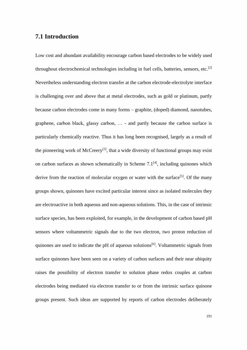
191
7.1 Introduction
Low cost and abundant availability encourage carbon based electrodes to be widely used
throughout electrochemical technologies including in fuel cells, batteries, sensors, etc.[2]
Nevertheless understanding electron transfer at the carbon electrode-electrolyte interface
is challenging over and above that at metal electrodes, such as gold or platinum, partly
because carbon electrodes come in many forms – graphite, (doped) diamond, nanotubes,
graphene, carbon black, glassy carbon, … - and partly because the carbon surface is
particularly chemically reactive. Thus it has long been recognised, largely as a result of
the pioneering work of McCreery[3], that a wide diversity of functional groups may exist
on carbon surfaces as shown schematically in Scheme 7.1[4], including quinones which
derive from the reaction of molecular oxygen or water with the surface[5]. Of the many
groups shown, quinones have excited particular interest since as isolated molecules they
are electroactive in both aqueous and non-aqueous solutions. This, in the case of intrinsic
surface species, has been exploited, for example, in the development of carbon based pH
sensors where voltammetric signals due to the two electron, two proton reduction of
quinones are used to indicate the pH of aqueous solutions[6]. Voltammetric signals from
surface quinones have been seen on a variety of carbon surfaces and their near ubiquity
raises the possibility of electron transfer to solution phase redox couples at carbon
electrodes being mediated via electron transfer to or from the intrinsic surface quinone
groups present. Such ideas are supported by reports of carbon electrodes deliberately
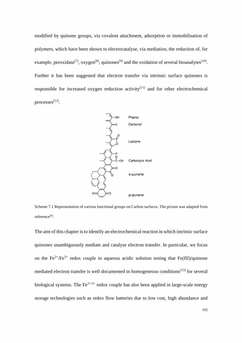
192
modified by quinone groups, via covalent attachment, adsorption or immobilisation of
polymers, which have been shown to electrocatalyse, via mediation, the reduction of, for
example, peroxidase[7], oxygen[8], quinones[9] and the oxidation of several bioanalytes[10].
Further it has been suggested that electron transfer via intrinsic surface quinones is
responsible for increased oxygen reduction activity[11] and for other electrochemical
processes[12].
Scheme 7.1 Representation of various functional groups on Carbon surfaces. The picture was adapted from
reference[8].
The aim of this chapter is to identify an electrochemical reaction in which intrinsic surface
quinones unambiguously mediate and catalyse electron transfer. In particular, we focus
on the Fe2+/Fe3+ redox couple in aqueous acidic solution noting that Fe(III)/quinone
mediated electron transfer is well documented in homogeneous conditions[13] for several
biological systems. The Fe2+/3+ redox couple has also been applied in large-scale energy
storage technologies such as redox flow batteries due to low cost, high abundance and
193
low chemical toxicity[14]. Accordingly the Fe2+/3+ system in the form of ca. milimolar
concentrations of NH4FeIII(SO4)2 and (NH4)2FeII(SO4)2 in 0.2 M HClO4 was investigated.
7.2 Experimental
7.2.1 Chemical reagents
The ammonium iron (II) sulfate hexahydrate ((NH4)2FeII(SO4)2; Aldrich; 99%),
ammonium iron (III) sulfate dodecahydrate (NH4FeIII(SO4)2; Aldrich; 99%), ammonium
sulfate ((NH4)2SO4; Aldrich; ≥99%), hexaammineruthenium (III) chloride
([Ru(NH3)6]Cl3, Alfa Aesar, ≥98.3%), potassium chloride (KCl, Sigma-Aldrich, ≥99.0%)
and perchloric acid (Aldrich; 70%) were used as purchased without further purification.
Solutions were prepared using deionised water (Milipore) with a resistivity of 18.2 MΩ
cm at 25 oC. Solutions containing Fe2+/3+ species were freshly prepared prior to
experiments.
7.2.2 Instrumentation
Electrochemical measurements were performed with a µAutolab Type III potentiostat
using a standard three electrode setup in an optimised thermostated electrochemical cell
as shown in Scheme 7.2(a). The details of this design are described in Chapter 24. A
carbon microdisc electrode (7 µm in diameter; BASi), a gold microdisc electrode (10 µm
in diameter; BASi) and a conventional carbon fibre microcylinder electrode (7 μm in
diameter; 0.890 mm in length; Scheme 7.2(b)) were used as working electrodes. The
194
carbon fibre microcylinder electrode was fabricated in-house using the method described
in Chapter 2. A saturated calomel electrode (SCE saturated KCl; BASi, Japan) and a
platinum wire were used as reference electrode and counter electrode, respectively. The
working disc electrodes were polished using alumina of decreasing size (1.0, 0.3 and 0.05
µm, Buehler, IL), washed with deionised water and dried with nitrogen prior to
experiments.
Scheme 7.2 (a) Schematic of the optimised thermostated electrochemical cell. The probe is used to sense
the temperature of the electrochemical cell, which is controlled by a Peltier. WE, RE and CE represent the
working electrode, reference electrode and counter electrode, respectively. (b) Schematic of a carbon fibre
microcylinder electrode.
7.2.3 Electrochemical measurements
All electrochemical measurements were conducted at 25 (± 0.1) oC inside a Faraday cage.
All the solutions were purged with nitrogen for at least 5 minutes before experiments.
Measurements of the formal potential and diffusion coefficients of the Fe2+/3+ redox
couple The formal potential was measured on a gold microdisc electrode (10 µm in
195
diameter; BASi) in a solution containing both Fe2+ and Fe3+ (5 mM NH4FeIII(SO4)2, 5
mM (NH4)2FeII(SO4)2, 2.5 mM (NH4)2SO4 in 0.2 M HClO4) at 0.05 V s-1. The diffusion
coefficients for Fe2+ and Fe3+ were measured on the same gold microdisc electrode at 0.01
V s-1 using different solutions (for Fe2+: 10 mM (NH4)2FeII(SO4)2 in 0.2 M HClO4; for
Fe3+: 10 mM NH4FeIII(SO4)2, 2.5 mM (NH4)2SO4 in 0.2 M HClO4).
Transfer experiments on a carbon microdisc electrode The adsorption isotherms for Fe2+
and Fe3+ were obtained by using solutions with variable concentrations of Fe2+ or Fe3+ for
“transfer experiments”. For each set of transfer experiment, the electrode was first
scanned in blank solution (2.5 mM (NH4)2SO4 in 0.2 M HClO4), the electrode was then
immersed in solutions of variable concentrations of Fe2+ or Fe3+ for 2 minutes and the
voltammetry was then measured in blank solution. Voltammograms for each
concentration were measured at both 0.2 V s-1 and 0.8 V s-1.
7.2.4 Simulation programmes
The voltammetric response of a 2D diffusion microdisc electrode was simulated using a
home-written programme written by Dr Oleksiy Klymenko based on the conformal
mapping of the spatial coordinates and uses an exponentially expanding time grid.[15]
7.3 Tafel analysis on a microdisc electrode
Tafel analysis provides a direct route by which the transfer coefficient for a redox reaction
can be determined. The transfer coefficient[16] is an experimentally measurable quantity
196
and is related to the fraction (and hence asymmetry) of the electrostatic potential available
for the oxidation or reduction process. Importantly, in the case of inner-sphere redox
reactions this fraction of the electrochemical potential available for the redox process can
be influenced by the electrode double layer.[17] Tafel analysis under different electrode
geometries has been discussed in Chapter 4. The anodic transfer coefficient (𝛼𝑎 ) is
defined by IUPAC as[16]:
𝛼𝑎 = (𝑅𝑇
𝐹) (
𝑑 ln 𝑗𝑎
𝑑𝐸) (7.1)
where 𝑗𝑎 is the anodic current density which has been corrected to account for changes
in the concentration of the reactant at the electrode surface, R is the gas constant (8.314 J
mol-1 K-1), T is the temperature in K, F is the Faraday constant (96485 C mol-1) and E is
the applied potential at the working electrode.
7.3.1 Mass-transport corrected transfer coefficient plots
For a carbon microdisc electrode at low scan rates a steady-state mass-transport regime
can be attained. However, the electrode surface is non-uniformly accessible which means
that, in contrast to other electrode geometries such as a hemispherical electrode, there is
no exact analytical expression available to correct for the influence of the mass-transport
conditions on the voltammetric response as discussed in Chapter 4. Consequently, the
correction made in this work to extract the transfer coefficient is strictly only approximate.
Specifically this work shows the estimation of experimental transfer coefficients on a
microdisc electrode via two different mass-transport corrections in the current range of 1%
197
to 95% of the steady-state current 𝐼𝑠.𝑠 or limiting current 𝐼𝑙𝑖𝑚. At high overpotentials,
the voltammetric current becomes mass-transport limited, which leads to an
underestimation of the transfer coefficient on a microelectrode. This first method for
correcting the measured transfer coefficient uses the analytically defined mass-transport
correction as derived in chapter 4, where the analytically mass-transport corrected anodic
transfer coefficient 𝛼𝑎′ was calculated using Equation 7.2[18].
−𝑅𝑇
𝐹
𝑑𝑙𝑛(1
𝐼𝑎−
1
𝐼𝑙𝑖𝑚)
𝑑𝐸= 𝛼𝑎
′ (7.2)
where 𝐼𝑙𝑖𝑚 is the mass-transport limiting current. For a microdisc electrode, the
theoretical steady-state current 𝐼𝑠.𝑠, calculated using Equation 7.3 was used as the mass-
transport limiting current throughout the analysis.
𝐼𝑠.𝑠 = 4𝑛𝐹𝐷𝑐𝑟 (7.3)
where 𝐼𝑠.𝑠 is the steady-state current, 𝑛 is the number of electrons transferred, 𝑐 is the
bulk concentration of the reactant, 𝐷 is the diffusion coefficient of the reactant and 𝑟 is
the radius of the electrode.
7.3.2 Non-uniformly mass-transport corrected transfer coefficient plots
The second method, a correction allowing for non-uniformly mass-transport was taken
into account to give a better estimation for the transfer coefficient. According to the
previous theoretical study reported in chapter 4, the mass-transport corrected transfer
coefficient plot on a microdisc electrode gives an improved measure of the transfer
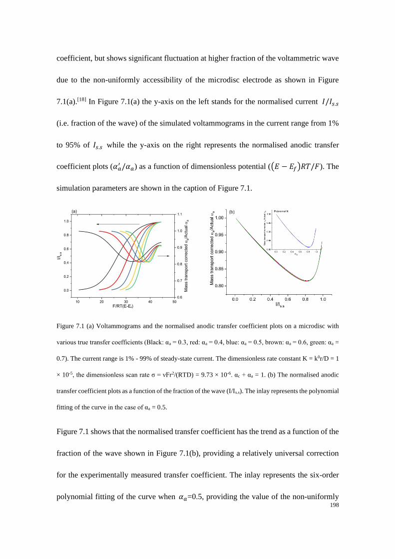
198
coefficient, but shows significant fluctuation at higher fraction of the voltammetric wave
due to the non-uniformly accessibility of the microdisc electrode as shown in Figure
7.1(a).[18] In Figure 7.1(a) the y-axis on the left stands for the normalised current 𝐼/𝐼𝑠.𝑠
(i.e. fraction of the wave) of the simulated voltammograms in the current range from 1%
to 95% of 𝐼𝑠.𝑠 while the y-axis on the right represents the normalised anodic transfer
coefficient plots (𝛼𝑎′ /𝛼𝑎) as a function of dimensionless potential ((𝐸 − 𝐸𝑓)𝑅𝑇/𝐹). The
simulation parameters are shown in the caption of Figure 7.1.
Figure 7.1 (a) Voltammograms and the normalised anodic transfer coefficient plots on a microdisc with
various true transfer coefficients (Black: αa = 0.3, red: αa = 0.4, blue: αa = 0.5, brown: αa = 0.6, green: αa =
0.7). The current range is 1% - 99% of steady-state current. The dimensionless rate constant K = k0r/D = 1
× 10-5, the dimensionless scan rate σ = νFr2/(RTD) = 9.73 × 10⁻⁶. αc + αa = 1. (b) The normalised anodic
transfer coefficient plots as a function of the fraction of the wave (I/Is.s). The inlay represents the polynomial
fitting of the curve in the case of αa = 0.5.
Figure 7.1 shows that the normalised transfer coefficient has the trend as a function of the
fraction of the wave shown in Figure 7.1(b), providing a relatively universal correction
for the experimentally measured transfer coefficient. The inlay represents the six-order
polynomial fitting of the curve when 𝛼𝑎=0.5, providing the value of the non-uniformly
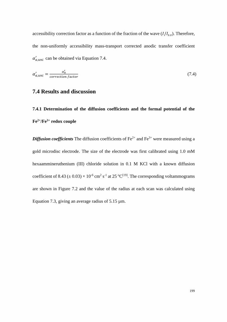
199
accessibility correction factor as a function of the fraction of the wave (𝐼/𝐼𝑠.𝑠). Therefore,
the non-uniformly accessibility mass-transport corrected anodic transfer coefficient
𝛼𝑎,𝑢𝑛𝑖′ can be obtained via Equation 7.4.
𝛼𝑎,𝑢𝑛𝑖′ =
𝛼𝑎′
𝑐𝑜𝑟𝑟𝑒𝑐𝑡𝑖𝑜𝑛 𝑓𝑎𝑐𝑡𝑜𝑟 (7.4)
7.4 Results and discussion
7.4.1 Determination of the diffusion coefficients and the formal potential of the
Fe2+/Fe3+ redox couple
Diffusion coefficients The diffusion coefficients of Fe2+ and Fe3+ were measured using a
gold microdisc electrode. The size of the electrode was first calibrated using 1.0 mM
hexaammineruthenium (III) chloride solution in 0.1 M KCl with a known diffusion
coefficient of 8.43 (± 0.03) × 10-6 cm2 s-1 at 25 oC[19]. The corresponding voltammograms
are shown in Figure 7.2 and the value of the radius at each scan was calculated using
Equation 7.3, giving an average radius of 5.15 µm.
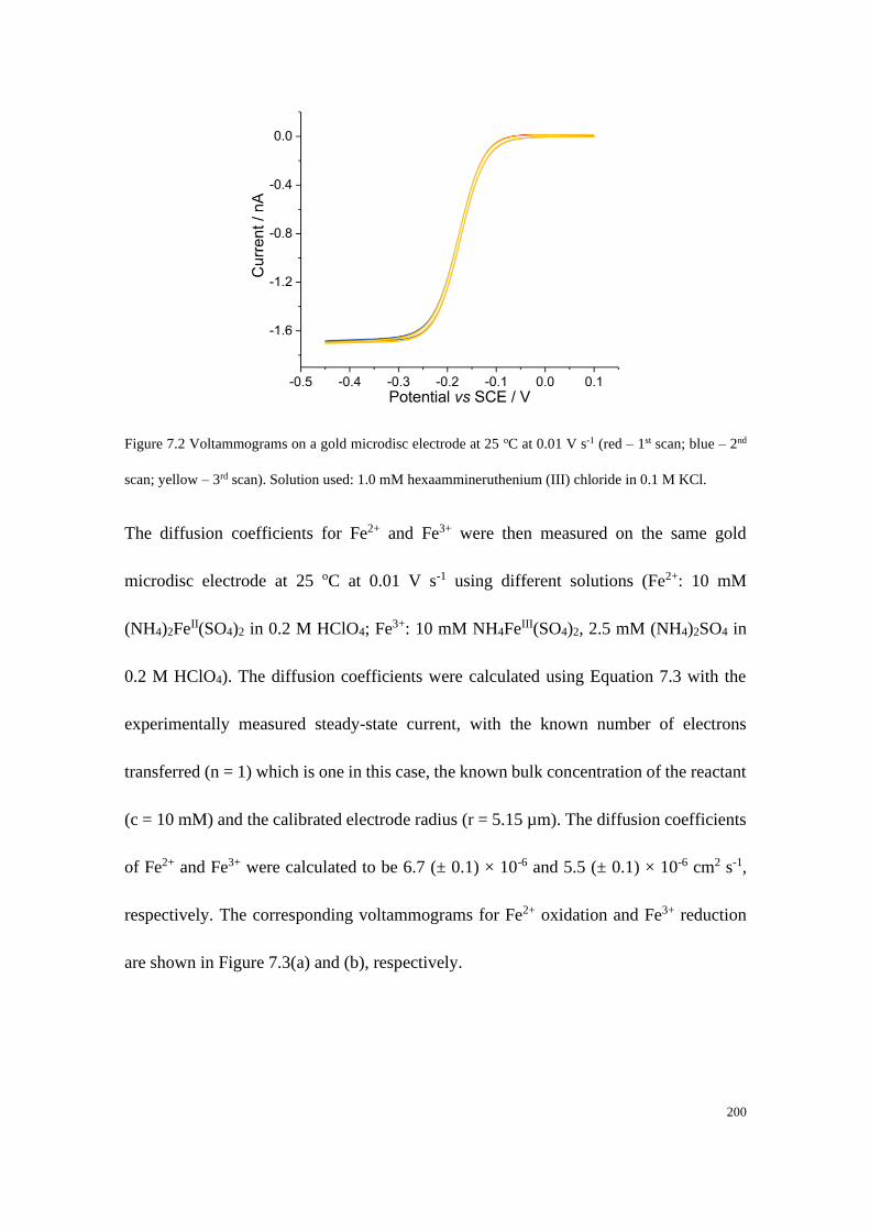
200
Figure 7.2 Voltammograms on a gold microdisc electrode at 25 oC at 0.01 V s-1 (red – 1st scan; blue – 2nd
scan; yellow – 3rd scan). Solution used: 1.0 mM hexaammineruthenium (III) chloride in 0.1 M KCl.
The diffusion coefficients for Fe2+ and Fe3+ were then measured on the same gold
microdisc electrode at 25 oC at 0.01 V s-1 using different solutions (Fe2+: 10 mM
(NH4)2FeII(SO4)2 in 0.2 M HClO4; Fe3+: 10 mM NH4FeIII(SO4)2, 2.5 mM (NH4)2SO4 in
0.2 M HClO4). The diffusion coefficients were calculated using Equation 7.3 with the
experimentally measured steady-state current, with the known number of electrons
transferred (n = 1) which is one in this case, the known bulk concentration of the reactant
(c = 10 mM) and the calibrated electrode radius (r = 5.15 µm). The diffusion coefficients
of Fe2+ and Fe3+ were calculated to be 6.7 (± 0.1) × 10-6 and 5.5 (± 0.1) × 10-6 cm2 s-1,
respectively. The corresponding voltammograms for Fe2+ oxidation and Fe3+ reduction
are shown in Figure 7.3(a) and (b), respectively.
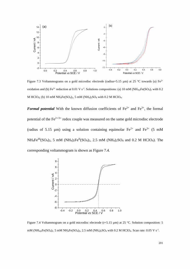
201
Figure 7.3 Voltammograms on a gold microdisc electrode (radius=5.15 µm) at 25 oC towards (a) Fe2+
oxidation and (b) Fe3+ reduction at 0.01 V s-1. Solutions compositions: (a) 10 mM (NH4)2Fe(SO4)2 with 0.2
M HClO4; (b) 10 mM NH4Fe(SO4)2, 5 mM (NH4)2SO4 with 0.2 M HClO4.
Formal potential With the known diffusion coefficients of Fe2+ and Fe3+, the formal
potential of the Fe2+/3+ redox couple was measured on the same gold microdisc electrode
(radius of 5.15 µm) using a solution containing equimolar Fe2+ and Fe3+ (5 mM
NH4FeIII(SO4)2, 5 mM (NH4)2FeII(SO4)2, 2.5 mM (NH4)2SO4 and 0.2 M HClO4). The
corresponding voltammogram is shown as Figure 7.4.
Figure 7.4 Voltammogram on a gold microdisc electrode (r=5.15 µm) at 25 oC. Solution composition: 5
mM (NH4)2Fe(SO4)2, 5 mM NH4Fe(SO4)2, 2.5 mM (NH4)2SO4 with 0.2 M HClO4. Scan rate: 0.05 V s-1.
-0.4 -0.2 0.0 0.2 0.4 0.6 0.8 1.0-8
-6
-4
-2
0
2
4
6
8
Cu
rre
nt
/ n
A
Potential vs SCE / V
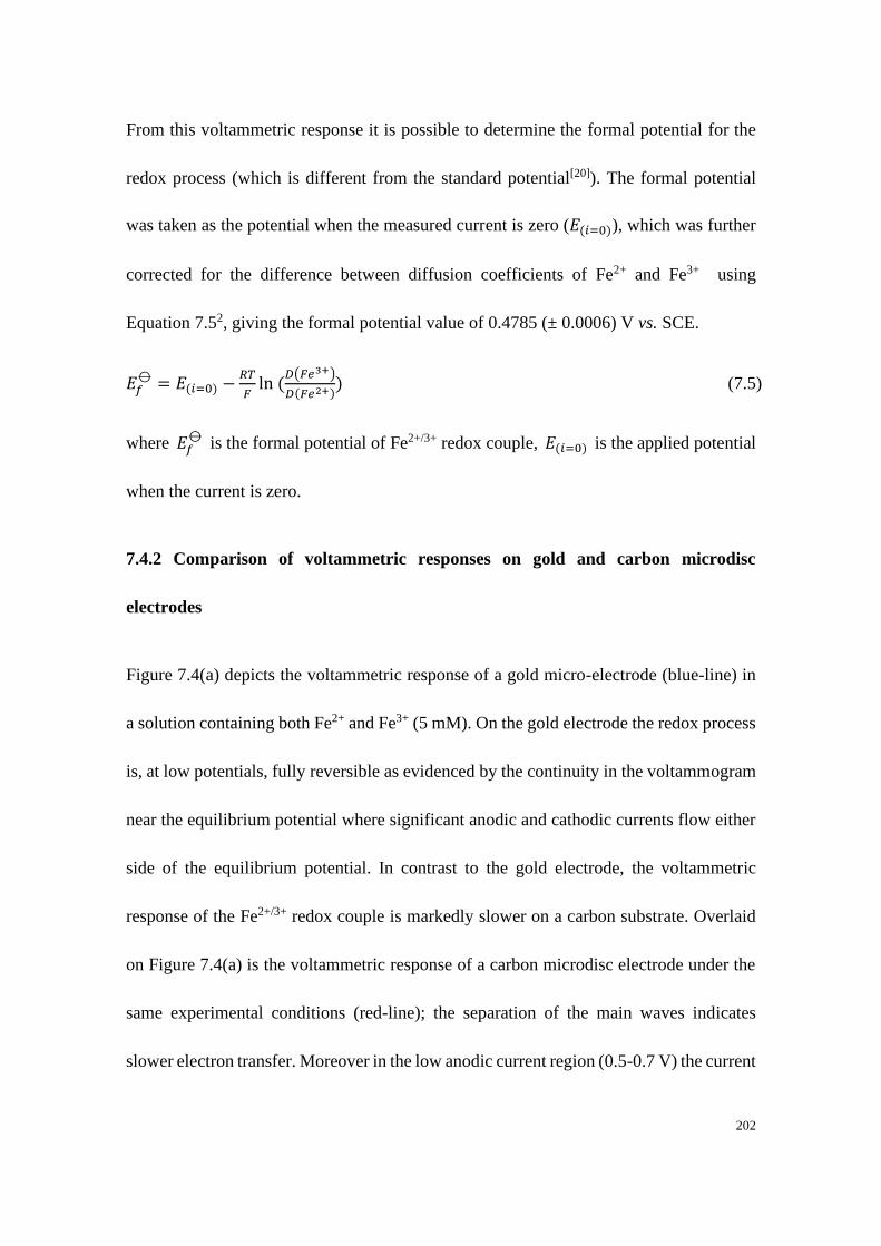
202
From this voltammetric response it is possible to determine the formal potential for the
redox process (which is different from the standard potential[20]). The formal potential
was taken as the potential when the measured current is zero (𝐸(𝑖=0)), which was further
corrected for the difference between diffusion coefficients of Fe2+ and Fe3+ using
Equation 7.52, giving the formal potential value of 0.4785 (± 0.0006) V vs. SCE.
𝐸𝑓⦵ = 𝐸(𝑖=0) −
𝑅𝑇
𝐹ln (
𝐷(𝐹𝑒3+)
𝐷(𝐹𝑒2+)) (7.5)
where 𝐸𝑓⦵
is the formal potential of Fe2+/3+ redox couple, 𝐸(𝑖=0) is the applied potential
when the current is zero.
7.4.2 Comparison of voltammetric responses on gold and carbon microdisc
electrodes
Figure 7.4(a) depicts the voltammetric response of a gold micro-electrode (blue-line) in
a solution containing both Fe2+ and Fe3+ (5 mM). On the gold electrode the redox process
is, at low potentials, fully reversible as evidenced by the continuity in the voltammogram
near the equilibrium potential where significant anodic and cathodic currents flow either
side of the equilibrium potential. In contrast to the gold electrode, the voltammetric
response of the Fe2+/3+ redox couple is markedly slower on a carbon substrate. Overlaid
on Figure 7.4(a) is the voltammetric response of a carbon microdisc electrode under the
same experimental conditions (red-line); the separation of the main waves indicates
slower electron transfer. Moreover in the low anodic current region (0.5-0.7 V) the current
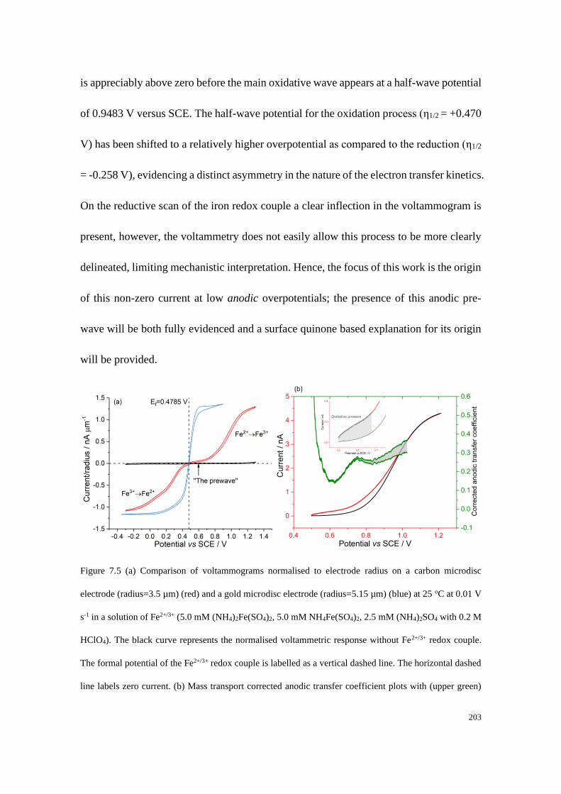
203
is appreciably above zero before the main oxidative wave appears at a half-wave potential
of 0.9483 V versus SCE. The half-wave potential for the oxidation process (η1/2 = +0.470
V) has been shifted to a relatively higher overpotential as compared to the reduction (η1/2
= -0.258 V), evidencing a distinct asymmetry in the nature of the electron transfer kinetics.
On the reductive scan of the iron redox couple a clear inflection in the voltammogram is
present, however, the voltammetry does not easily allow this process to be more clearly
delineated, limiting mechanistic interpretation. Hence, the focus of this work is the origin
of this non-zero current at low anodic overpotentials; the presence of this anodic pre-
wave will be both fully evidenced and a surface quinone based explanation for its origin
will be provided.
Figure 7.5 (a) Comparison of voltammograms normalised to electrode radius on a carbon microdisc
electrode (radius=3.5 µm) (red) and a gold microdisc electrode (radius=5.15 µm) (blue) at 25 oC at 0.01 V
s-1 in a solution of Fe2+/3+ (5.0 mM (NH4)2Fe(SO4)2, 5.0 mM NH4Fe(SO4)2, 2.5 mM (NH4)2SO4 with 0.2 M
HClO4). The black curve represents the normalised voltammetric response without Fe2+/3+ redox couple.
The formal potential of the Fe2+/3+ redox couple is labelled as a vertical dashed line. The horizontal dashed
line labels zero current. (b) Mass transport corrected anodic transfer coefficient plots with (upper green)
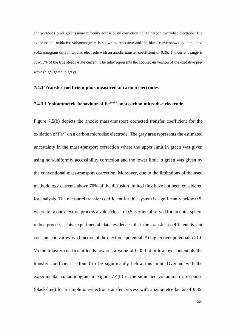
204
and without (lower green) non-uniformly accessibility correction on the carbon microdisc electrode. The
experimental oxidative voltammogram is shown as red curve and the black curve shows the simulated
voltammogram on a microdisc electrode with an anodic transfer coefficient of 0.35. The current range is
1%-95% of the true steady-state current. The inlay represents the zoomed-in version of the oxidative pre-
wave (highlighted in grey).
7.4.3 Transfer coefficient plots measured at carbon electrodes
7.4.3.1 Voltammetric behaviour of Fe2+/3+ on a carbon microdisc electrode
Figure 7.5(b) depicts the anodic mass-transport corrected transfer coefficient for the
oxidation of Fe2+ on a carbon microdisc electrode. The gray area represents the estimated
uncertainty in the mass-transport correction where the upper limit in green was given
using non-uniformly accessibility correction and the lower limit in green was given by
the conventional mass-transport correction. Moreover, due to the limitations of the used
methodology currents above 70% of the diffusion limited flux have not been considered
for analysis. The measured transfer coefficient for this system is significantly below 0.5,
where for a one electron process a value close to 0.5 is often observed for an outer sphere
redox process. This experimental data evidences that the transfer coefficient is not
constant and varies as a function of the electrode potential. At higher over potentials (>1.0
V) the transfer coefficient tends towards a value of 0.35 but at low over potentials the
transfer coefficient is found to be significantly below this limit. Overlaid with the
experimental voltammogram in Figure 7.4(b) is the simulated voltammetric response
(black-line) for a simple one-electron transfer process with a symmetry factor of 0.35.
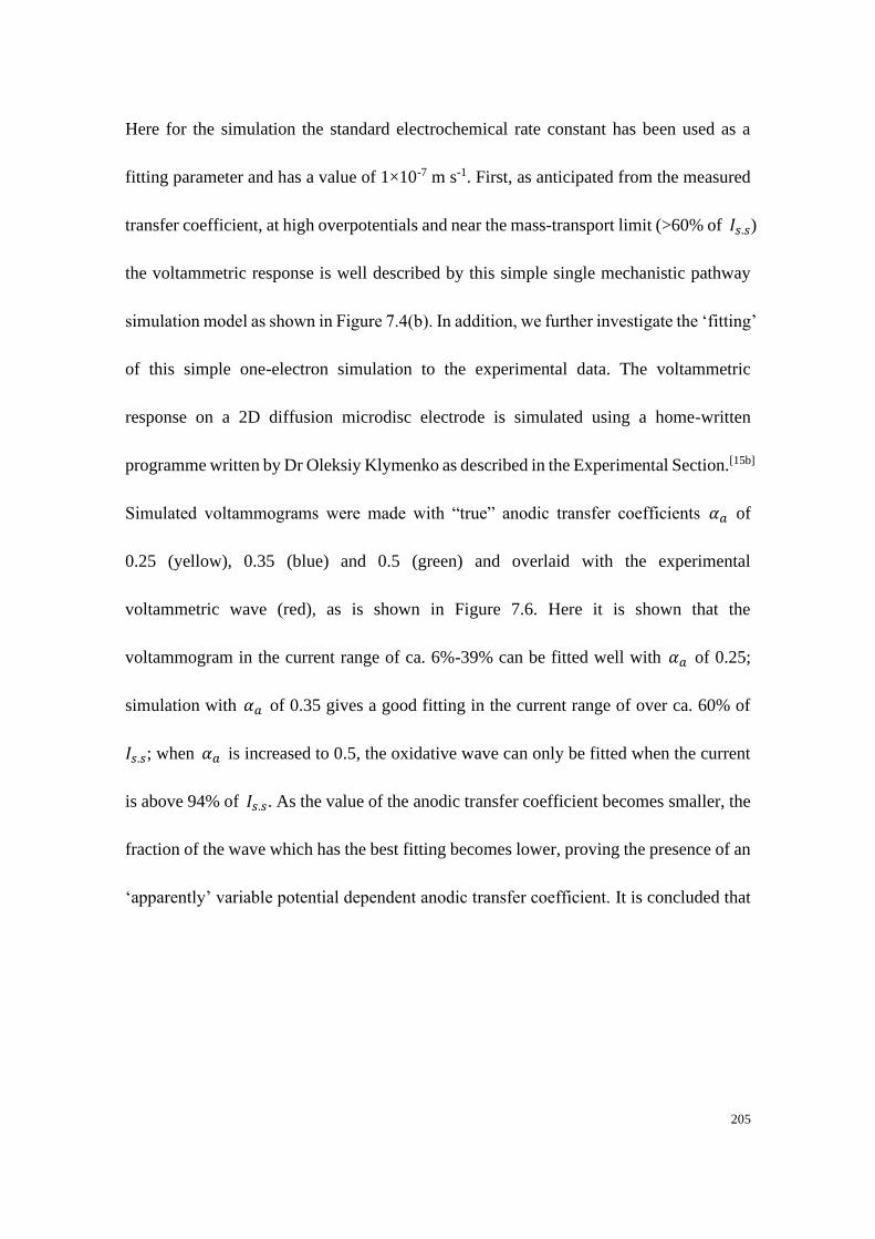
205
Here for the simulation the standard electrochemical rate constant has been used as a
fitting parameter and has a value of 1×10⁻⁷ m s-1. First, as anticipated from the measured
transfer coefficient, at high overpotentials and near the mass-transport limit (>60% of 𝐼𝑠.𝑠)
the voltammetric response is well described by this simple single mechanistic pathway
simulation model as shown in Figure 7.4(b). In addition, we further investigate the ‘fitting’
of this simple one-electron simulation to the experimental data. The voltammetric
response on a 2D diffusion microdisc electrode is simulated using a home-written
programme written by Dr Oleksiy Klymenko as described in the Experimental Section.[15b]
Simulated voltammograms were made with “true” anodic transfer coefficients 𝛼𝑎 of
0.25 (yellow), 0.35 (blue) and 0.5 (green) and overlaid with the experimental
voltammetric wave (red), as is shown in Figure 7.6. Here it is shown that the
voltammogram in the current range of ca. 6%-39% can be fitted well with 𝛼𝑎 of 0.25;
simulation with 𝛼𝑎 of 0.35 gives a good fitting in the current range of over ca. 60% of
𝐼𝑠.𝑠; when 𝛼𝑎 is increased to 0.5, the oxidative wave can only be fitted when the current
is above 94% of 𝐼𝑠.𝑠. As the value of the anodic transfer coefficient becomes smaller, the
fraction of the wave which has the best fitting becomes lower, proving the presence of an
‘apparently’ variable potential dependent anodic transfer coefficient. It is concluded that
206
no fixed single value of the transfer coefficient is able to fit the experimental current
across the full range of potentials.
Figure 7.6 Fitting of the experimental voltammogram (red) using the simulations with different anodic
transfer coefficients on a microdisc electrode (yellow: 𝛼𝑎 =0.25; blue: 𝛼𝑎 =0.35; green: 𝛼𝑎 =0.5).
Parameters used in the simulation: scan rate=0.01 V s-1; D(Fe2+)=6.68×10⁻¹⁰ m2 s-1; D(Fe3+)=5.45×10⁻¹⁰ m2
s-1; electron transfer rate=1×10⁻⁷ m s-1, the formal potential=0.4837 V.
7.4.3.2 Voltammetric behaviour of Fe2+/3+ on a carbon micro-wire electrode
The measured change in the transfer coefficient as a function of the applied potential on
a carbon microdisc electrode is first strongly indicative of a change in the electrochemical
redox mechanism with potential. Second, as evidenced through comparison of the
simulated and experimental data, at low overpotentials there is more current passed than
would be expected for a simple electron transfer process. For the microdisc electrode
geometry a “pre-wave” contributes approximately 0.2 nA of current and for clarity has
been highlighted in the inlay of Figure 7.4(b). Moreover, for other electrode geometries
where the mass-transport regime is less efficient this pre-wave becomes relatively larger.
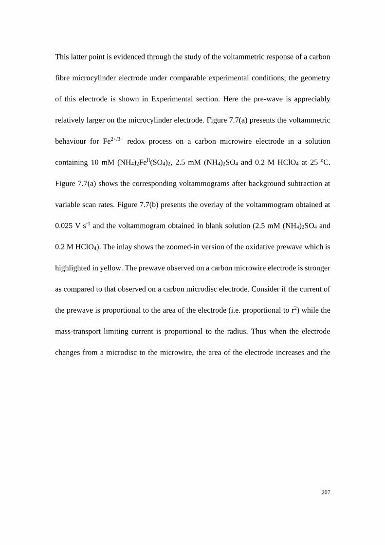
207
This latter point is evidenced through the study of the voltammetric response of a carbon
fibre microcylinder electrode under comparable experimental conditions; the geometry
of this electrode is shown in Experimental section. Here the pre-wave is appreciably
relatively larger on the microcylinder electrode. Figure 7.7(a) presents the voltammetric
behaviour for Fe2+/3+ redox process on a carbon microwire electrode in a solution
containing 10 mM (NH4)2FeII(SO4)2, 2.5 mM (NH4)2SO4 and 0.2 M HClO4 at 25 oC.
Figure 7.7(a) shows the corresponding voltammograms after background subtraction at
variable scan rates. Figure 7.7(b) presents the overlay of the voltammogram obtained at
0.025 V s-1 and the voltammogram obtained in blank solution (2.5 mM (NH4)2SO4 and
0.2 M HClO4). The inlay shows the zoomed-in version of the oxidative prewave which is
highlighted in yellow. The prewave observed on a carbon microwire electrode is stronger
as compared to that observed on a carbon microdisc electrode. Consider if the current of
the prewave is proportional to the area of the electrode (i.e. proportional to r2) while the
mass-transport limiting current is proportional to the radius. Thus when the electrode
changes from a microdisc to the microwire, the area of the electrode increases and the
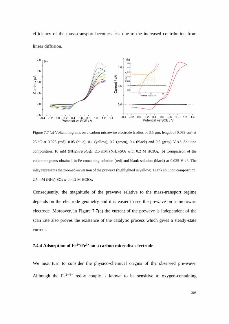
208
efficiency of the mass-transport becomes less due to the increased contribution from
linear diffusion.
Figure 7.7 (a) Voltammograms on a carbon microwire electrode (radius of 3.5 µm; length of 0.089 cm) at
25 oC at 0.025 (red), 0.05 (blue), 0.1 (yellow), 0.2 (green), 0.4 (black) and 0.8 (gray) V s-1. Solution
composition: 10 mM (NH4)2Fe(SO4)2, 2.5 mM (NH4)2SO4 with 0.2 M HClO4. (b) Comparison of the
voltammograms obtained in Fe-containing solution (red) and blank solution (black) at 0.025 V s-1. The
inlay represents the zoomed-in version of the prewave (highlighted in yellow). Blank solution composition:
2.5 mM (NH4)2SO4 with 0.2 M HClO4.
Consequently, the magnitude of the prewave relative to the mass-transport regime
depends on the electrode geometry and it is easier to see the prewave on a microwire
electrode. Moreover, in Figure 7.7(a) the current of the prewave is independent of the
scan rate also proves the existence of the catalytic process which gives a steady-state
current.
7.4.4 Adsorption of Fe2+/Fe3+ on a carbon microdisc electrode
We next turn to consider the physico-chemical origins of the observed pre-wave.
Although the Fe2+/3+ redox couple is known to be sensitive to oxygen-containing
209
functional groups on the electrode surface[3a, 3b], it has not been proved which specific
functional groups are responsible for the catalysed reaction. The origin of the interaction
between Fe ions and the functional groups which results in the occurrence of pre-wave
was next investigated. Transfer experiments were conducted to study possible adsorption
behaviour.
7.4.4.1 Fe3+ reduction on a carbon microdisc electrode
A carbon microdisc was immersed into a solution containing certain concentration of
NH4FeIII(SO4)2, 2.5 mM (NH4)2SO4 in 0.2 M HClO4, and the voltammetric response of
this interface studied before and after exposure to the solution. The voltammetric
experiments were measured in the absence of Fe(III) in the solution phase; procedures
are provided in the Experimental Section. Figure 7.8(a) depicts examples of the measured
voltammetric response of the electrode before (red-line) and after (black-line) immersion
in the iron containing solution. For the clean carbon surface the voltammetric response of
the electrode exhibits a relatively large capacitative charging current and at a pH of 0.69,
a broad surface bound feature corresponding to the redox chemistry of surface quinone
groups (at ca.0.38 V vs SCE)[6a]. From this voltammetric peak the surface coverage of
catechol on a clean carbon electrode was calculated to be (4.33 ± 0.66) × 10-11 mol cm-2
as ascertained from the integration of the quinone/catechol peak observed in blank
solution. This value is consistent with the literature values for ortho-quinones measured
on basal plane and edge plane pyrolytic graphite electrodes of 1.7 × 10⁻¹⁰ and 2.0 × 10⁻¹²
210
mol cm-2, respectively[21]. After exposure of the electrode to the Fe(II) containing solution
an additional redox signal is observed at ca. 0.54 V versus SCE. The presence of this
additional redox feature can be more fully resolved by background subtraction. Figure
7.8(b) shows the voltammetric response of the electrode exposed to the iron solution
where variable iron concentrations have been used after removal of the capacitive and
quinone responses by subtracting the voltammograms in blank solution. The
voltammograms give well-defined surface-bound peaks at around 0.5 V in all cases; the
peak charge increases with the increasing Fe3+ concentration in the range of 5 mM to 20
mM and becomes essentially constant when the Fe3+ concentration is larger than 20 mM.
First, the charge passed oxidatively and reductively, is comparable and indicates that both
the oxidised and reduced iron species remain adsorbed to the electrode surface on the
voltammetric timescale. Second, integration of the peak enables the surface coverage of
the adsorbed iron to be assessed as depicted in the inlay in Figure 7.8 which presents the
measured Fe3+ adsorption isotherm on the carbon microdisc electrode in solutions
containing variable concentrations of Fe3+. The experimentally measured maximum
surface coverage of adsorbed Fe3+ was calculated to be (4.42 ± 0.18) × 10-11 mol cm-2,
which is very comparable to that expected from surface quinones. The consistency
between the surface coverages of quinone/catechol and the Fe3+ ions strongly indicates
that the occurrence of the additional peaks is attributed to Fe2+/3+ adsorption on the
electrode. In addition, the prewave was observed at lower overpotential compared to the
main oxidative wave which means that such process is easier to happen, indicating a
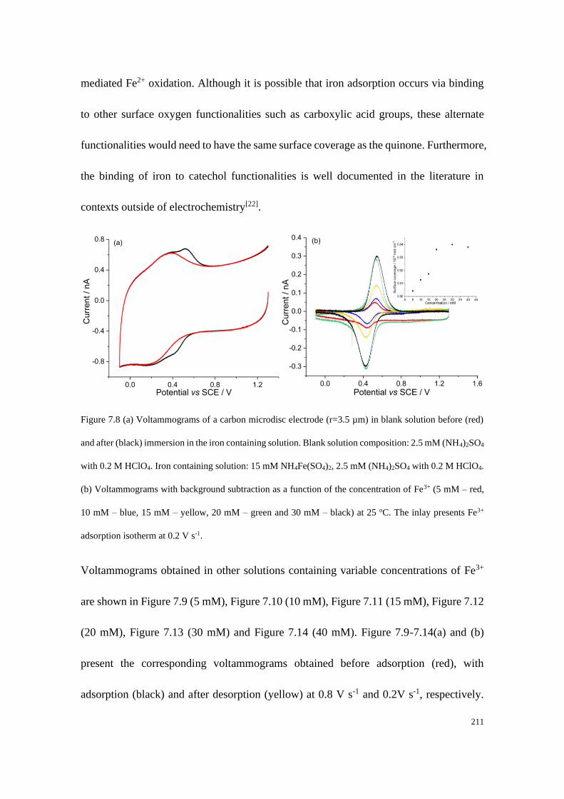
211
mediated Fe2+ oxidation. Although it is possible that iron adsorption occurs via binding
to other surface oxygen functionalities such as carboxylic acid groups, these alternate
functionalities would need to have the same surface coverage as the quinone. Furthermore,
the binding of iron to catechol functionalities is well documented in the literature in
contexts outside of electrochemistry[22].
Figure 7.8 (a) Voltammograms of a carbon microdisc electrode (r=3.5 µm) in blank solution before (red)
and after (black) immersion in the iron containing solution. Blank solution composition: 2.5 mM (NH4)2SO4
with 0.2 M HClO4. Iron containing solution: 15 mM NH4Fe(SO4)2, 2.5 mM (NH4)2SO4 with 0.2 M HClO4.
(b) Voltammograms with background subtraction as a function of the concentration of Fe3+ (5 mM – red,
10 mM – blue, 15 mM – yellow, 20 mM – green and 30 mM – black) at 25 oC. The inlay presents Fe3+
adsorption isotherm at 0.2 V s-1.
Voltammograms obtained in other solutions containing variable concentrations of Fe3+
are shown in Figure 7.9 (5 mM), Figure 7.10 (10 mM), Figure 7.11 (15 mM), Figure 7.12
(20 mM), Figure 7.13 (30 mM) and Figure 7.14 (40 mM). Figure 7.9-7.14(a) and (b)
present the corresponding voltammograms obtained before adsorption (red), with
adsorption (black) and after desorption (yellow) at 0.8 V s-1 and 0.2V s-1, respectively.
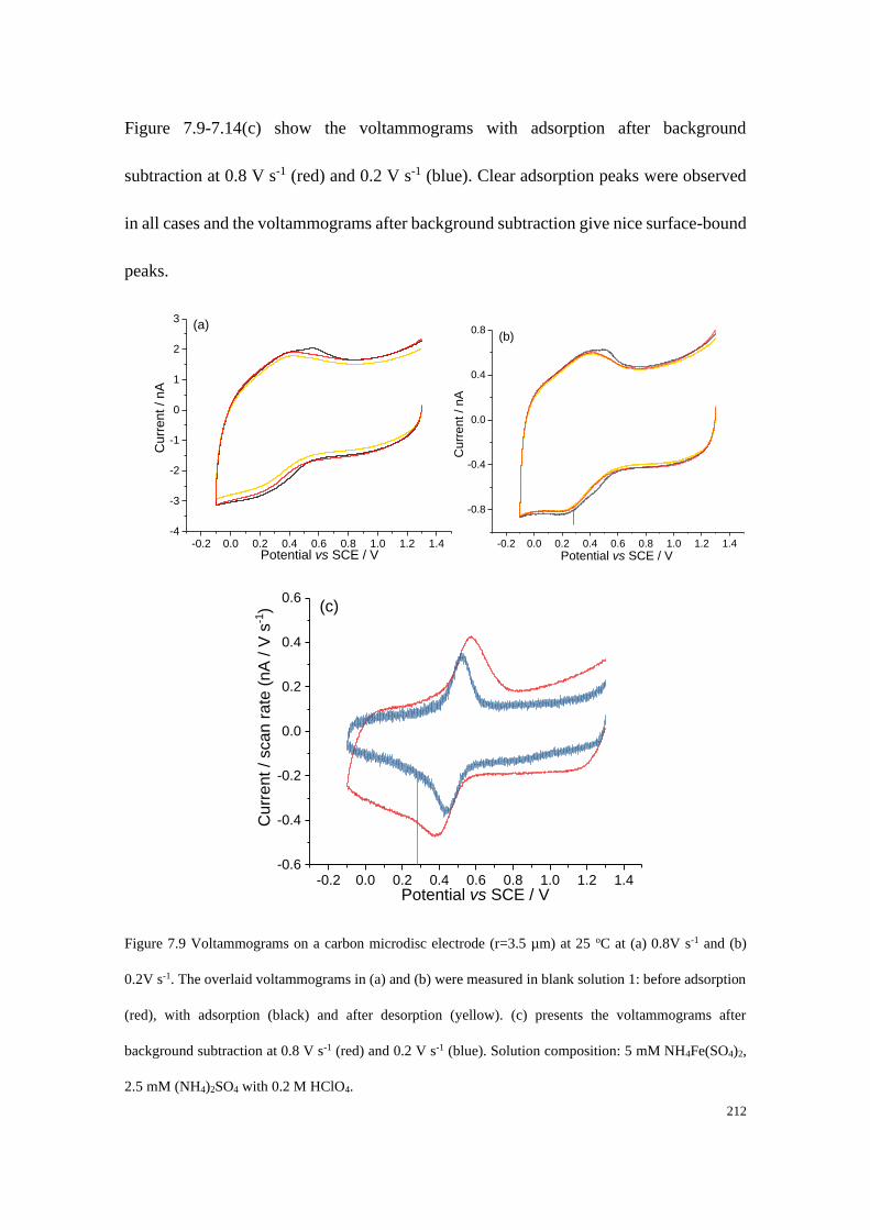
212
Figure 7.9-7.14(c) show the voltammograms with adsorption after background
subtraction at 0.8 V s-1 (red) and 0.2 V s-1 (blue). Clear adsorption peaks were observed
in all cases and the voltammograms after background subtraction give nice surface-bound
peaks.
Figure 7.9 Voltammograms on a carbon microdisc electrode (r=3.5 µm) at 25 oC at (a) 0.8V s-1 and (b)
0.2V s-1. The overlaid voltammograms in (a) and (b) were measured in blank solution 1: before adsorption
(red), with adsorption (black) and after desorption (yellow). (c) presents the voltammograms after
background subtraction at 0.8 V s-1 (red) and 0.2 V s-1 (blue). Solution composition: 5 mM NH4Fe(SO4)2,
2.5 mM (NH4)2SO4 with 0.2 M HClO4.
-0.2 0.0 0.2 0.4 0.6 0.8 1.0 1.2 1.4-4
-3
-2
-1
0
1
2
3
Cu
rre
nt
/ n
A
Potential vs SCE / V
(a)
-0.2 0.0 0.2 0.4 0.6 0.8 1.0 1.2 1.4
-0.8
-0.4
0.0
0.4
0.8(b)
Cu
rre
nt
/ n
A
Potential vs SCE / V
-0.2 0.0 0.2 0.4 0.6 0.8 1.0 1.2 1.4-0.6
-0.4
-0.2
0.0
0.2
0.4
0.6(c)
Cu
rrent / scan
rate
(nA
/ V
s-1
)
Potential vs SCE / V
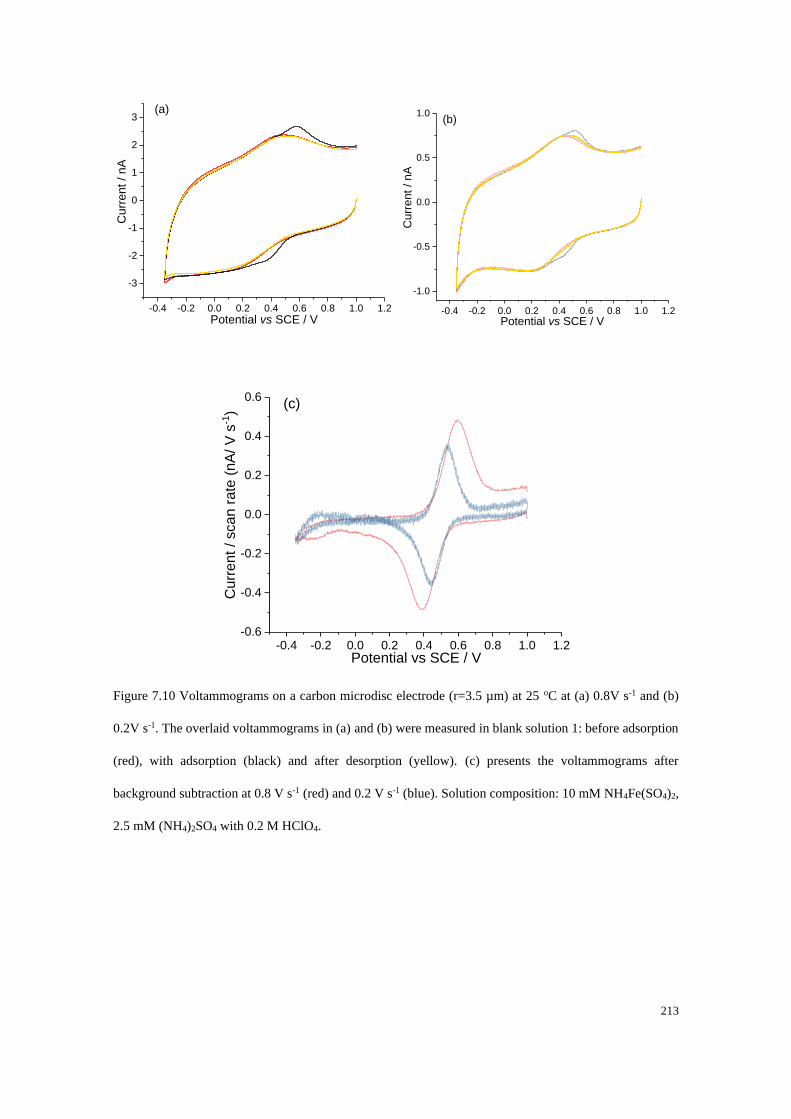
213
Figure 7.10 Voltammograms on a carbon microdisc electrode (r=3.5 µm) at 25 oC at (a) 0.8V s-1 and (b)
0.2V s-1. The overlaid voltammograms in (a) and (b) were measured in blank solution 1: before adsorption
(red), with adsorption (black) and after desorption (yellow). (c) presents the voltammograms after
background subtraction at 0.8 V s-1 (red) and 0.2 V s-1 (blue). Solution composition: 10 mM NH4Fe(SO4)2,
2.5 mM (NH4)2SO4 with 0.2 M HClO4.
-0.4 -0.2 0.0 0.2 0.4 0.6 0.8 1.0 1.2
-3
-2
-1
0
1
2
3C
urr
en
t / n
A
Potential vs SCE / V
(a)
-0.4 -0.2 0.0 0.2 0.4 0.6 0.8 1.0 1.2
-1.0
-0.5
0.0
0.5
1.0
Cu
rrent / nA
Potential vs SCE / V
(b)
-0.4 -0.2 0.0 0.2 0.4 0.6 0.8 1.0 1.2-0.6
-0.4
-0.2
0.0
0.2
0.4
0.6
Cu
rre
nt
/ sca
n r
ate
(n
A/
V s
-1)
Potential vs SCE / V
(c)
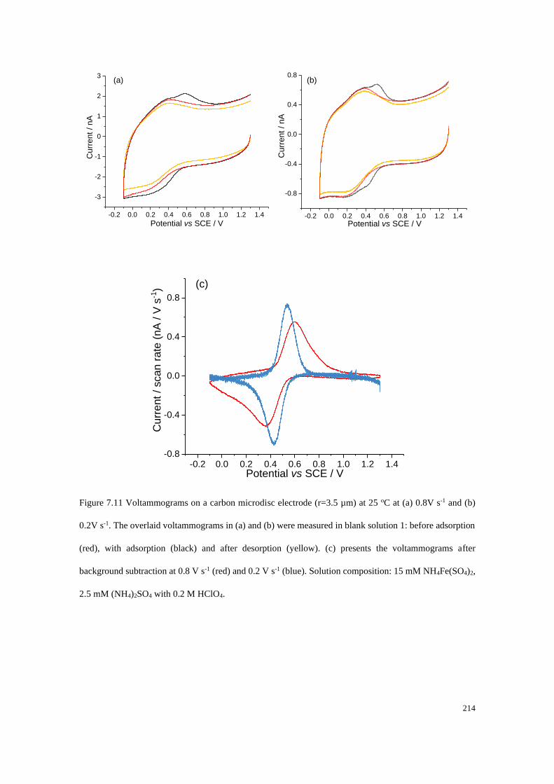
214
Figure 7.11 Voltammograms on a carbon microdisc electrode (r=3.5 µm) at 25 oC at (a) 0.8V s-1 and (b)
0.2V s-1. The overlaid voltammograms in (a) and (b) were measured in blank solution 1: before adsorption
(red), with adsorption (black) and after desorption (yellow). (c) presents the voltammograms after
background subtraction at 0.8 V s-1 (red) and 0.2 V s-1 (blue). Solution composition: 15 mM NH4Fe(SO4)2,
2.5 mM (NH4)2SO4 with 0.2 M HClO4.
-0.2 0.0 0.2 0.4 0.6 0.8 1.0 1.2 1.4
-3
-2
-1
0
1
2
3
Cu
rre
nt
/ n
A
Potential vs SCE / V
(a)
-0.2 0.0 0.2 0.4 0.6 0.8 1.0 1.2 1.4
-0.8
-0.4
0.0
0.4
0.8
Cu
rre
nt
/ n
A
Potential vs SCE / V
(b)
-0.2 0.0 0.2 0.4 0.6 0.8 1.0 1.2 1.4-0.8
-0.4
0.0
0.4
0.8
Cu
rrent / scan
rate
(nA
/ V
s-1
)
Potential vs SCE / V
(c)
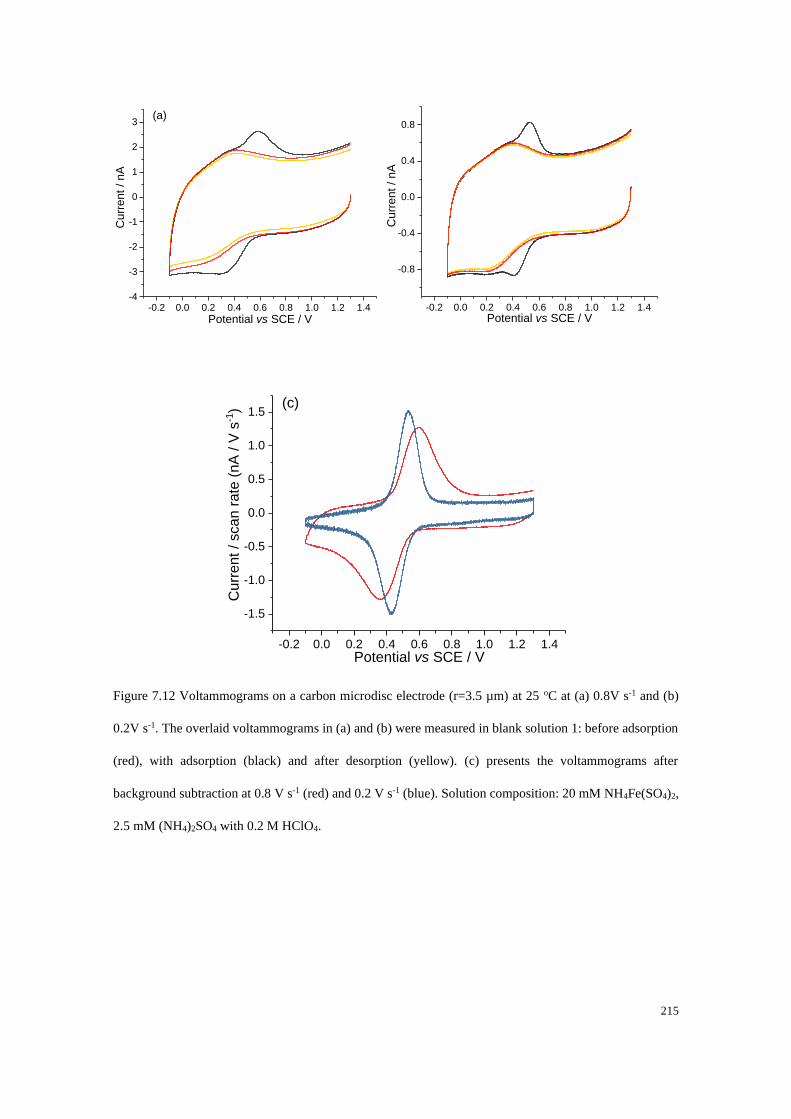
215
Figure 7.12 Voltammograms on a carbon microdisc electrode (r=3.5 µm) at 25 oC at (a) 0.8V s-1 and (b)
0.2V s-1. The overlaid voltammograms in (a) and (b) were measured in blank solution 1: before adsorption
(red), with adsorption (black) and after desorption (yellow). (c) presents the voltammograms after
background subtraction at 0.8 V s-1 (red) and 0.2 V s-1 (blue). Solution composition: 20 mM NH4Fe(SO4)2,
2.5 mM (NH4)2SO4 with 0.2 M HClO4.
-0.2 0.0 0.2 0.4 0.6 0.8 1.0 1.2 1.4-4
-3
-2
-1
0
1
2
3C
urr
ent / nA
Potential vs SCE / V
(a)
-0.2 0.0 0.2 0.4 0.6 0.8 1.0 1.2 1.4
-0.8
-0.4
0.0
0.4
0.8
Cu
rrent / nA
Potential vs SCE / V
-0.2 0.0 0.2 0.4 0.6 0.8 1.0 1.2 1.4
-1.5
-1.0
-0.5
0.0
0.5
1.0
1.5
Cu
rrent / scan
rate
(nA
/ V
s-1
)
Potential vs SCE / V
(c)
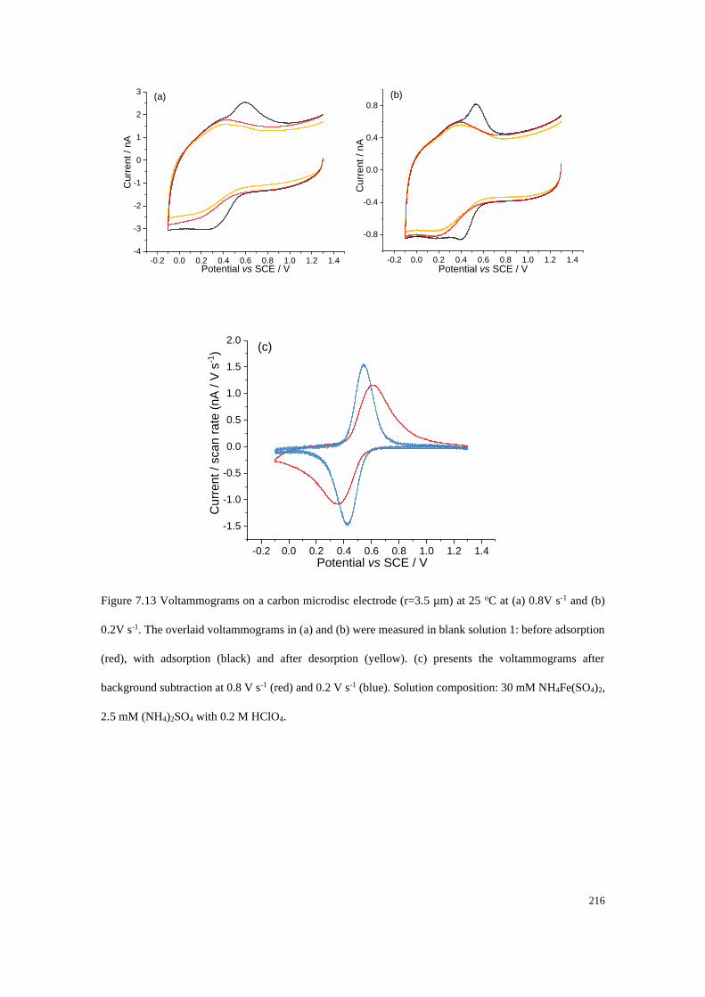
216
Figure 7.13 Voltammograms on a carbon microdisc electrode (r=3.5 µm) at 25 oC at (a) 0.8V s-1 and (b)
0.2V s-1. The overlaid voltammograms in (a) and (b) were measured in blank solution 1: before adsorption
(red), with adsorption (black) and after desorption (yellow). (c) presents the voltammograms after
background subtraction at 0.8 V s-1 (red) and 0.2 V s-1 (blue). Solution composition: 30 mM NH4Fe(SO4)2,
2.5 mM (NH4)2SO4 with 0.2 M HClO4.
-0.2 0.0 0.2 0.4 0.6 0.8 1.0 1.2 1.4-4
-3
-2
-1
0
1
2
3
Cu
rrent / nA
Potential vs SCE / V
(a)
-0.2 0.0 0.2 0.4 0.6 0.8 1.0 1.2 1.4
-0.8
-0.4
0.0
0.4
0.8
Cu
rre
nt
/ n
A
Potential vs SCE / V
(b)
-0.2 0.0 0.2 0.4 0.6 0.8 1.0 1.2 1.4
-1.5
-1.0
-0.5
0.0
0.5
1.0
1.5
2.0
Cu
rrent / scan
rate
(nA
/ V
s-1
)
Potential vs SCE / V
(c)

217
Figure 7.14 Voltammograms on a carbon microdisc electrode (r=3.5 µm) at 25 oC at (a) 0.8V s-1 and (b)
0.2V s-1. The overlaid voltammograms in (a) and (b) were measured in blank solution 1: before adsorption
(red), with adsorption (black) and after desorption (yellow). (c) presents the voltammograms after
background subtraction at 0.8 V s-1 (red) and 0.2 V s-1 (blue). Solution composition: 40 mM NH4Fe(SO4)2,
2.5 mM (NH4)2SO4 with 0.2 M HClO4.
7.4.4.2 Fe2+ oxidation on a carbon microdisc electrode
Similar experiments to those reported above were undertaken to investigate Fe2+
adsorption on carbon electrodes. The polished carbon microdisc electrode was first
-0.2 0.0 0.2 0.4 0.6 0.8 1.0 1.2 1.4-4
-3
-2
-1
0
1
2
3
Cu
rre
nt
/ n
A
Potential vs SCE / V
(a)
-0.2 0.0 0.2 0.4 0.6 0.8 1.0 1.2 1.4
-1.0
-0.5
0.0
0.5
1.0
Cu
rrent / nA
Potential vs SCE / V
(b)
-0.2 0.0 0.2 0.4 0.6 0.8 1.0 1.2 1.4-2.0
-1.5
-1.0
-0.5
0.0
0.5
1.0
1.5
Cu
rre
nt
/ sca
n r
ate
(n
A /
V s
-1)
Potential vs SCE / V
(c)
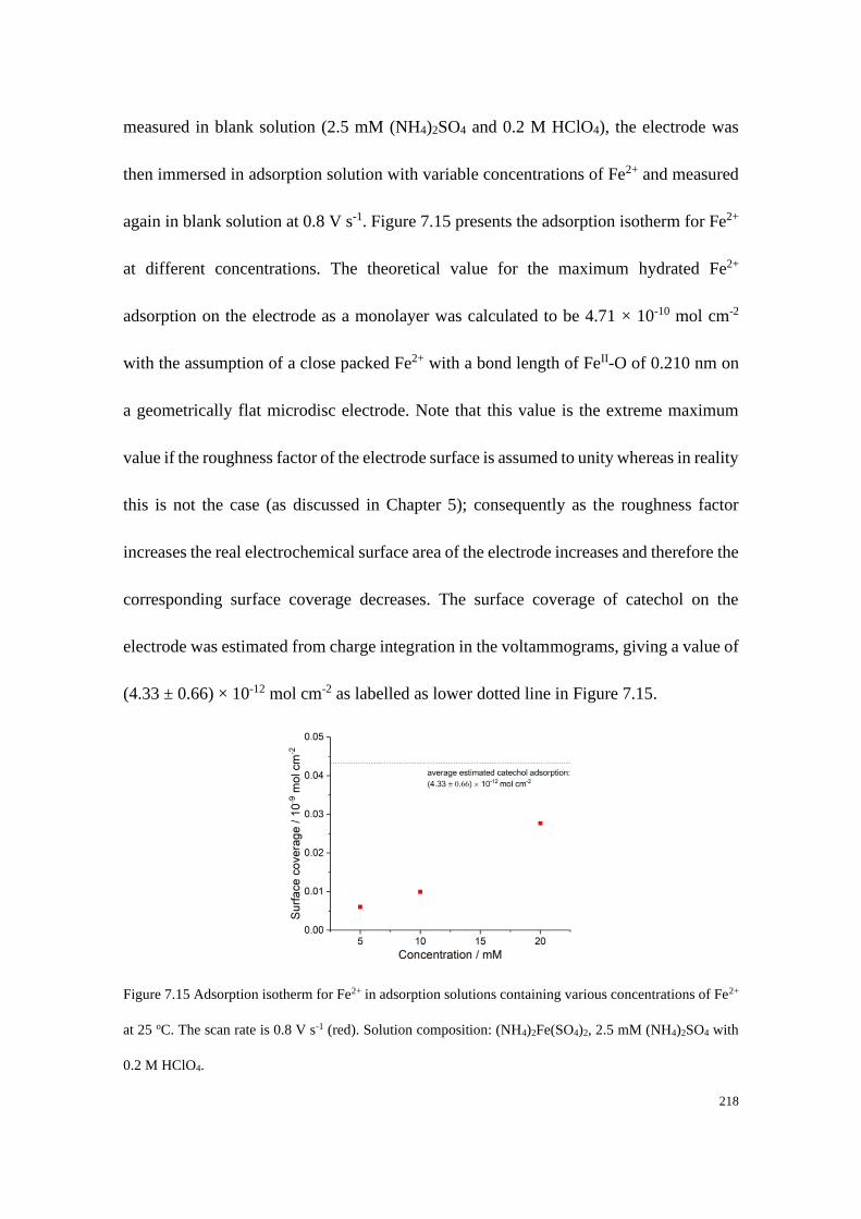
218
measured in blank solution (2.5 mM (NH4)2SO4 and 0.2 M HClO4), the electrode was
then immersed in adsorption solution with variable concentrations of Fe2+ and measured
again in blank solution at 0.8 V s-1. Figure 7.15 presents the adsorption isotherm for Fe2+
at different concentrations. The theoretical value for the maximum hydrated Fe2+
adsorption on the electrode as a monolayer was calculated to be 4.71 × 10⁻¹⁰ mol cm-2
with the assumption of a close packed Fe2+ with a bond length of FeII-O of 0.210 nm on
a geometrically flat microdisc electrode. Note that this value is the extreme maximum
value if the roughness factor of the electrode surface is assumed to unity whereas in reality
this is not the case (as discussed in Chapter 5); consequently as the roughness factor
increases the real electrochemical surface area of the electrode increases and therefore the
corresponding surface coverage decreases. The surface coverage of catechol on the
electrode was estimated from charge integration in the voltammograms, giving a value of
(4.33 ± 0.66) × 10-12 mol cm-2 as labelled as lower dotted line in Figure 7.15.
Figure 7.15 Adsorption isotherm for Fe2+ in adsorption solutions containing various concentrations of Fe2+
at 25 oC. The scan rate is 0.8 V s-1 (red). Solution composition: (NH4)2Fe(SO4)2, 2.5 mM (NH4)2SO4 with
0.2 M HClO4.

219
The corresponding voltammograms for Fe2+ transfer experiments in each concentration,
5 mM (Figure 7.16), 10 mM (Figure 7.17) and 20 mM (Figure 7.18) are shown below.
Figure 7.16 - 7.18(a) present the corresponding voltammograms obtained in blank
solution before adsorption (red), with adsorption (black) and after desorption (yellow) at
0.8 V s-1. Figure 7.16-7.18(b) show the voltammograms with adsorption after background
subtraction at 0.8 V s-1. Similarly, clear adsorption peaks were observed in all cases and
the voltammograms after background subtraction give nice surface-bound peaks, which
further indicates that the Fe2+/Fe3+ redox couple is sensitive to the presence of
quinone/catechol groups.
Figure 7.16 (a) Voltammograms on a carbon microdisc electrode (r=3.5 µm) at 25 oC at 0.8V s-1. The
overlaid voltammograms in (a) were measured in blank solution 1: before adsorption (red), with adsorption
(black) and after desorption (yellow). (b) presents the voltammograms after background subtraction at 0.8
V s-1. Solution composition: 5 mM (NH4)2Fe(SO4)2 with 0.2 M HClO4.
-0.2 0.0 0.2 0.4 0.6 0.8 1.0 1.2 1.4-3
-2
-1
0
1
2
3
Cu
rrent / nA
Potential vs SCE / V
(a)
-0.2 0.0 0.2 0.4 0.6 0.8 1.0 1.2 1.4
-0.2
-0.1
0.0
0.1
0.2
Cu
rre
nt
/ n
A
Potential vs SCE / V
(b)
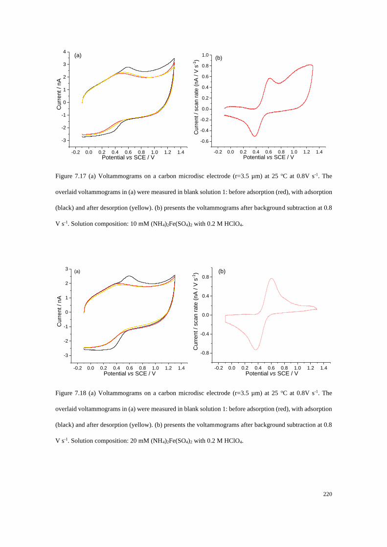
220
Figure 7.17 (a) Voltammograms on a carbon microdisc electrode (r=3.5 µm) at 25 oC at 0.8V s-1. The
overlaid voltammograms in (a) were measured in blank solution 1: before adsorption (red), with adsorption
(black) and after desorption (yellow). (b) presents the voltammograms after background subtraction at 0.8
V s-1. Solution composition: 10 mM (NH4)2Fe(SO4)2 with 0.2 M HClO4.
Figure 7.18 (a) Voltammograms on a carbon microdisc electrode (r=3.5 µm) at 25 oC at 0.8V s-1. The
overlaid voltammograms in (a) were measured in blank solution 1: before adsorption (red), with adsorption
(black) and after desorption (yellow). (b) presents the voltammograms after background subtraction at 0.8
V s-1. Solution composition: 20 mM (NH4)2Fe(SO4)2 with 0.2 M HClO4.
-0.2 0.0 0.2 0.4 0.6 0.8 1.0 1.2 1.4
-3
-2
-1
0
1
2
3
4
Cu
rrent / nA
Potential vs SCE / V
(a)
-0.2 0.0 0.2 0.4 0.6 0.8 1.0 1.2 1.4
-0.6
-0.4
-0.2
0.0
0.2
0.4
0.6
0.8
1.0
Cu
rre
nt
/ sca
n r
ate
(n
A /
V s
-1)
Potential vs SCE / V
(b)
-0.2 0.0 0.2 0.4 0.6 0.8 1.0 1.2 1.4
-3
-2
-1
0
1
2
3
Cu
rrent / nA
Potential vs SCE / V
(a)
-0.2 0.0 0.2 0.4 0.6 0.8 1.0 1.2 1.4
-0.8
-0.4
0.0
0.4
0.8
Cu
rre
nt
/ sca
n r
ate
(n
A /
V s
-1)
Potential vs SCE / V
(b)
221
7.4.5 Proposed mechanistic model of the Fe2+/3+ redox process
The pre-wave observed on the carbon electrode in Figure 7.4 gives a quasi-steady-state-
like behaviour. Such steady-state behaviour was also observed by Sato et al. in the
investigation of the catalysis of the oxidation of Fe2+ in aqueous solution by [Mo(CN)8]3-
on a rotating disk pyrolytic graphite electrode[23]. On the basis of the above experimental
results we propose that the Fe2+ oxidation on the carbon electrode can be understood via
a mechanistic model involving two parallel pathways (Scheme 7.3). First, at low
overpotentials there is a surface mediated redox reaction where the results are consistent
with the oxidation proceeding via a surface adsorbed iron-quinone complex (Pathway 1)
and the current obtained from pathway 1 is labelled as 𝐼1. Second, at higher overpotentials
the oxidation proceeds via a direct solution phase oxidative route (Pathway 2) and the
obtained current from this pathway is 𝐼2. Here, for pathway 𝐼1 the likely rate determining
step will be desorption of the Fe3+ species. However, it should however be noted that an
alternative reaction scheme whereby the surface adsorbed iron species serves to mediate
the electron transfer in a manner comparable to that found for the self-catalysis of
catechol[9] cannot be ruled out. Moreover, it is more challenging to conceive of how such
a mechanism could lead to the occurrence of two parallel electron transfer pathways, as
experimentally evidenced by the measured transfer coefficient. The transfer coefficient
for this direct oxidative pathway (𝐼2) has a value of approximately 0.35, as determined
from the experimental data at high overpotentials whilst the value is much smaller at low
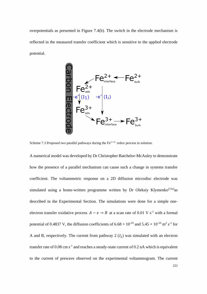
222
overpotentials as presented in Figure 7.4(b). The switch in the electrode mechanism is
reflected in the measured transfer coefficient which is sensitive to the applied electrode
potential.
Scheme 7.3 Proposed two parallel pathways during the Fe2+/3+ redox process in solution.
A numerical model was developed by Dr Christopher Batchelor-McAuley to demonstrate
how the presence of a parallel mechanism can cause such a change in systems transfer
coefficient. The voltammetric response on a 2D diffusion microdisc electrode was
simulated using a home-written programme written by Dr Oleksiy Klymenko[15a]as
described in the Experimental Section. The simulations were done for a simple one-
electron transfer oxidative process 𝐴 − 𝑒 → 𝐵 at a scan rate of 0.01 V s-1 with a formal
potential of 0.4837 V, the diffusion coefficients of 6.68 × 10⁻¹⁰ and 5.45 × 10⁻¹⁰ m2 s-1 for
A and B, respectively. The current from pathway 2 (𝐼2) was simulated with an electron
transfer rate of 0.08 cm s-1 and reaches a steady-state current of 0.2 nA which is equivalent
to the current of prewave observed on the experimental voltammogram. The current
223
obtained under diffusion-only condition from pathway 1 (𝐼1) was simulated with an
anodic transfer coefficient 𝛼𝑎 of 0.35 (𝛼𝑎 + 𝛼𝑐 = 1), an electron transfer rate of 1×10⁻⁵
cm s-1 and the electrode radius of 3.51 µm. The total voltammetric current was then
estimated using mathematical approximation using Equation (7.4) and the corresponding
voltammogram is shown in Figure 7.19(a). In the analytical approximation, 𝐼2
𝐼𝑠.𝑠 stands for
the amount of materials consumed by pathway 2 and (1 −𝐼2
𝐼𝑠.𝑠) then represents for the
amount of materials left for the pathway 1. Figure 7.19(b) shows the oxidative transfer
coefficient plot in the current range of 1%-95% of 𝐼𝑠.𝑠 with (green curve) and without
(red curve) mass-transport correction. It shows that the non-mass-transport corrected
anodic transfer coefficient significantly deviates from its true value (0.35) and approaches
zero at high overpotential. The range of the transfer coefficient was given as the gray-
shaded area where the upper limit was given using non-uniformly accessibility correction
and the lower limit was given by the conventional mass-transport correction and the
darker colour represents larger probability to its true value. As is shown in Figure 7.19(b),
the corrected transfer coefficient drops down for both correction methods when the
current range is larger than ca. 70% of 𝐼𝑠.𝑠 due to the increased contribution from linear
diffusion and therefore the larger deviation from a true steady-state condition.
𝐼𝑡𝑜𝑡 = 𝐼2 + (1 −𝐼2
𝐼𝑠.𝑠)𝐼1 (7.6)

224
Figure 7.19 (a) Simulated voltammetric responses (𝐼1-red; 𝐼2-blue; 𝐼𝑡𝑜𝑡 -yellow) on a carbon microdisc
electrode for the proposed two parallel model. (b) Anodic transfer coefficient plots for the oxidative wave
in the current range of 1%-95% of 𝐼𝑠.𝑠 . The yellow curve is the oxidative wave. The red curve is the
measured anodic transfer coefficient plot without mass transport correction. The green curves are the mass-
transport corrected transfer coefficient with (upper green curve) and without (lower green curve) non-
uniformly accessibility correction. The estimated range of the transfer coefficient is shaded where the
darker colour gives a closer to its true value.
7.5 Conclusions
To conclude, the surface quinones on carbon electrodes were found to intrinsically alter
Fe2+ oxidation via the formation of Fe-quinone complexes under acidic conditions. Such
mediation has long been suggested but not proved. This quinone mediated redox process
was observed as a quasi-steady-state like ‘prewave’ at lower overpotential compared to
the main wave on a carbon microdisc electrode. Moreover, the presence of this
electrocatalytic process (i.e. the pre-wave) is more apparent under lower mass-transport
conditions and will likely be the dominant redox pathway when larger macroscale
electrodes are used, as may be employed for example in a redox flow-cell battery.

225
References:
[1] D. Li, C. Batchelor-McAuley, L. Chen, R. G. Compton, The Journal of Physical Chemistry Letters
2020, 11, 1497-1501.
[2] aL. Yue, W. Li, F. Sun, L. Zhao, L. Xing, Carbon 2010, 48, 3079-3090; bL.-C. Jiang, W.-D.
Zhang, Biosensors and Bioelectronics 2010, 25, 1402-1407; cY. Zhang, L. Liu, B. Van der
Bruggen, F. Yang, Journal of Materials Chemistry A 2017, 5, 12673-12698.
[3] aP. Chen, M. A. Fryling, R. L. McCreery, Analytical Chemistry 1995, 67, 3115-3122; bP. Chen,
R. L. McCreery, Analytical Chemistry 1996, 68, 3958-3965; cR. L. McCreery, Chemical reviews
2008, 108, 2646-2687.
[4] A. J. Bard, Electroanalytical Chemistry: A Series of Advances, Taylor & Francis, 1990.
[5] K. Chaisiwamongkhol, C. Batchelor‐McAuley, R. G. Palgrave, R. G. Compton, Angewandte
Chemie 2018, 130, 6378-6381.
[6] aK. Chaisiwamongkhol, C. Batchelor-McAuley, R. G. Compton, Analyst 2017, 142, 2828-2835;
bM. Lu, R. G. Compton, Analyst 2014, 139, 2397-2403.
[7] J. C. Hoogvliet, P. Van Os, E. J. Van der Mark, W. P. Van Bennekom, Biosensors and
Bioelectronics 1991, 6, 413-423.
[8] aA. Sarapuu, K. Helstein, D. J. Schiffrin, K. Tammeveski, Electrochemical and Solid State Letters
2004, 8, E30; bK. Tammeveski, K. Kontturi, R. J. Nichols, R. J. Potter, D. J. Schiffrin, Journal of
Electroanalytical Chemistry 2001, 515, 101-112.
[9] S. H. DuVall, R. L. McCreery, Journal of the American Chemical Society 2000, 122, 6759-6764.
[10] S. Chakraborty, C. R. Raj, Journal of Electroanalytical Chemistry 2007, 609, 155-162.
[11] T. Nagaoka, T. Sakai, K. Ogura, T. Yoshino, Analytical Chemistry 1986, 58, 1953-1955.
[12] J. Zhang, X. Wang, Q. Su, L. Zhi, A. Thomas, X. Feng, D. S. Su, R. Schlogl, K. Mullen, Journal
of the American Chemical Society 2009, 131, 11296-11297.
[13] aX. Li, T. Liu, L. Liu, F. Li, RSC Advances 2014, 4, 2284-2290; bX. Li, L. Liu, T. Liu, T. Yuan,
W. Zhang, F. Li, S. Zhou, Y. Li, Chemosphere 2013, 92, 218-224; cW. D. Burgos, Y. Fang, R. A.
Royer, G.-T. Yeh, J. J. Stone, B.-H. Jeon, B. A. Dempsey, Geochimica et cosmochimica acta 2003,
67, 2735-2748; dY. Wu, F. Li, T. Liu, R. Han, X. Luo, Electrochimica Acta 2016, 213, 408-415.
[14] aT. J. Petek, N. C. Hoyt, R. F. Savinell, J. S. Wainright, Journal of Power Sources 2015, 294, 620-
626; bL. Wei, M. C. Wu, T. S. Zhao, Y. K. Zeng, Y. X. Ren, Applied Energy 2018, 215, 98-105.
[15] aO. V. Klymenko, R. G. Evans, C. Hardacre, I. B. Svir, R. G. Compton, Journal of
Electroanalytical Chemistry 2004, 571, 211-221; bO. Klymenko, R. G. Compton, Thesis
(D.Phil.)--University of Oxford, 2004. 2004.
[16] aR. Guidelli, R. G. Compton, J. M. Feliu, E. Gileadi, J. Lipkowski, W. Schmickler, S. Trasatti,
Pure and Applied Chemistry 2014, 86, 259-262; bR. Guidelli, R. G. Compton, J. M. Feliu, E.
Gileadi, J. Lipkowski, W. Schmickler, S. Trasatti, Pure and Applied Chemistry 2014, 86, 245-258.
[17] E. Gileadi, Journal of Solid State Electrochemistry 2011, 15, 1359.
[18] D. Li, C. Lin, C. Batchelor-McAuley, L. Chen, R. G. Compton, Journal of Electroanalytical
Chemistry 2018, 826, 117-124.

226
[19] K. Ngamchuea, C. Lin, C. Batchelor-McAuley, R. G. Compton, Analytical Chemistry 2017, 89,
3780-3786.
[20] D. Li, C. Batchelor-McAuley, R. G. Compton, Applied Materials Today 2019.
[21] C. A. Thorogood, G. G. Wildgoose, A. Crossley, R. M. J. Jacobs, J. H. Jones, R. G. Compton,
Chemistry of Materials 2007, 19, 4964-4974.
[22] aM. J. Harrington, A. Masic, N. Holten-Andersen, J. H. Waite, P. Fratzl, Science 2010, 328, 216-
220; bN. Holten-Andersen, M. J. Harrington, H. Birkedal, B. P. Lee, P. B. Messersmith, K. Y. C.
Lee, J. H. Waite, Proceedings of the National Academy of Sciences 2011, 108, 2651-2655.
[23] K. Sato, T. Ohsaka, H. Matsuda, N. Oyama, Bulletin of the Chemical Society of Japan 1983, 56,
1863-1864.
227
Chapter 8
Mass Transport Corrected Transfer Coefficients from
Microdisc Cyclic Voltammetry: 2D Simulation and
Experiment
The transfer coefficient (or equivalently the Tafel slope) is an experimentally measurable
parameter defined as the change in the logarithm of the current density as a function of
the applied potential, where the current density has been corrected for changes in the
concentration of the reagent at the interface. For some electrode geometries (such as the
rotating disc or a micro hemispherical electrode) where the electroactive interface is
uniformly accessible under a steady-state regime, these changes in concentration can be
corrected for analytically which significantly increases the potential range over which
Tafel analysis can be used to accurately yield information regarding the electron transfer
process as discussed in Chapters 4 and 5. The important question arises therefore, for non-
uniformly accessible electrodes, such as a microdisc, where the current density varies
across the electrode surface, how can the experimentally measured electrochemical flux
be corrected for to account for the changes in the surface concentration of the reagent?
This work presents a simple simulation technique that allows the voltammetry of a
microdisc to be ‘mass-transport’ corrected without recourse to the use of analytical
approximations.

228
This work presented in this chapter has been published in ChemElectroChem and was
carried out in collaboration with Dr. Christopher Batchelor-McAuley.
8.1 Introduction
Tafel analysis allows the experimental determination of the sensitivity of an interfacial
redox reaction to the applied electrode potential.[1] This sensitivity is often expressed as
a Tafel slope (b = dE/dlog|i|) with units of mV dec-1 or equivalently as a transfer
coefficient (α = RTln10/Fb). However, as the overpotential for a redox reaction increases,
the interfacial electron transfer rapidly becomes limited by the mass-transport of the
reactant to the interface and not the kinetics of the electrochemical reaction. This issue of
the mass-transport limitation of the reaction rate significantly constrains the range over
which Tafel analysis can be performed on a voltammogram so as to allow the extraction
of physically meaningful insight regarding the electron transfer kinetics. Reflecting this
issue of the mass-transport limitation, the International Union of Pure and Applied
Chemistry (IUPAC) have more rigorously defined the transfer coefficient (𝛼𝑐 ) for a
reductive (cathodic) process as:[2]
𝛼𝑐 = −𝑅𝑇
𝐹(
𝑑𝑙𝑛|𝑗𝑐,𝑐𝑜𝑟𝑟|
𝑑𝐸) (8.1)
where R is the gas constant (8.314 J K mol-1), T is the temperature (298.15 K), F is the
Faraday Constant (96485 C mol-1) and E is the applied potential at the working electrode
(V) and the cathodic flux (𝑗𝑐,𝑐𝑜𝑟𝑟) has been corrected for any changes in the reactant
229
concentration at the electrode surface with respect to its bulk value. Similarly, the anodic
transfer coefficient is defined simply as above in Equation (8.1) but where the minus sign
is removed and 𝑗𝑐,𝑐𝑜𝑟𝑟 is replaced by the anodic flux (𝑗𝑎,𝑐𝑜𝑟𝑟).
This definition of transfer coefficient is independent of any mechanistic considerations;
consequently, having experimentally determined the transfer coefficient, so as to gain
insight into the interfacial process, it is for the researcher to interpret the physical meaning
of the measured value. In the case where only one electron is being transferred, then the
transfer coefficient can in this case be viewed as the fraction of the electrostatic potential
difference ‘driving’ the reaction which is available to affect the interfacial reaction rate,
such that the transfer coefficient serves to give a measure of the ‘position’ - reactant- or
product-like - of the transition state.[3] In this one-electron case it is generally assumed
that the transfer coefficient will have a value close to 0.5; however, for electrochemical
reactions involving adsorbed species the transfer coefficient can deviate significantly
away from this value.[4] Further in accordance with the Butler-Volmer equation it is
commonly assumed that the transfer coefficient is a constant, independent of the applied
electrode potential. As outlined by Marcus-Hush theory, which provides a microscopic
model for an outer-sphere electron transfer process, the transfer coefficient is anticipated
to tend to zero at high overpotentials[5]. Marcus-Hush theory rationalises the electron
transfer rate in terms of the reaction Gibbs energy and a ‘reorganisation energy’. So-called
‘Symmetric’ Marcus-Hush theory, as originally employed by Chidsey and others,
assumes the force constants for the reduced and oxidised species are equal. Consequently,
230
this symmetric formulation is equivalent to assuming that at low overpotentials the
transfer coefficient is equal to 0.5.[6] However, in reality even for outer-sphere redox
processes, and as mentioned above, the transfer coefficient often deviates from 0.5.[7]
Correspondence between Marcus-Hush Theory and the Butler-Volmer equation can be
found by allowing the force constants for the reduced and oxidised species to differ.[8]
This ‘asymmetric’ formulation of the Marcus-Hush theory provides a more realistic
microscopic model of the outer-sphere interfacial redox process, such that the Butler-
Volmer equation can be viewed as providing (in the low overpotential limit) an accurate
but approximate description of the sensitivity of the electron transfer rate to the applied
electrode potential. Further for outer sphere redox processes the transfer coefficient may
thus be interpreted as reflecting the asymmetry in the force constants of the reduced and
oxidised species. For the situation in which either multiple electrons are transferred and
or the interfacial electron transfer reaction is coupled to a homogeneous chemical process
then the interpretation of the transfer coefficient becomes appreciably more complex[9].
However, broadly in this case the transfer coefficient can be viewed as being a measure
of the number of electrons transferred prior to transition state of the rate determining
step.[10] Experimentally, the kinetics of interfacial charge transfer reactions have been
demonstrated to deviate significantly from this Butler-Volmer relation, evidencing the
potential dependence of the transfer coefficient as a function of the applied potential.[11]
Early work by Savéant and his co-workers demonstrated that for a series of outer-sphere
elementary electron transfer processes involving the redox of organic molecules in aprotic
231
media at a mercury electrode, the experimentally determined variation in the transfer
coefficient was comparable in magnitude to that predicted by Marcus theory.[11b, 11c] Other
work involving potential dependent transfer coefficient have been observed in coupled
electron-proton transfer with surface attached redox couples.[12] Hence, although
commonly employed the assumption that the transfer coefficient is a constant is not
physically correct. However, the largest discrepancies between Butler-Volmer kinetics
and Marcus-Hush theory is anticipated to occur at high overpotentials but it is precisely
this region of interest that is commonly under mass-transport control, thus limiting the
ability of Tafel analysis to successfully differentiate between these electron transfer
models.
For a fully irreversible reductive process, when the applied potential is sufficiently far
from the equilibrium potential Eeq, the flux contribution from the oxidation can be
neglected. In this case and at low current densities the transfer coefficient can be
experimentally measured[13] without considering the concentration changes of the electro-
active species at the interface:
−𝑅𝑇
𝐹
𝑑𝑙𝑛|𝐼𝑐|
𝑑𝐸= 𝛼𝑐,𝑛𝑐 (8.2)
where 𝐼𝑐 is the experimentally measured cathodic current, 𝛼𝑐,𝑛𝑐 is the non-mass-
transport corrected transfer coefficients. Hence, the measured transfer coefficient 𝛼𝑐,𝑛𝑐
will, at higher potentials, deviate from its true value 𝛼𝑐 (given by equation 8.1) due to
the local depletion of reagents at the electrochemical interface. At low current densities
232
(relative to the mass-transport limit) this issue of reactant depletion is not significant and
in this case 𝛼𝑐,𝑛𝑐 → 𝛼𝑐 and a plot of 𝑙𝑛|𝐼| vs E should have a slope equal to −𝛼𝑐𝐹/𝑅𝑇.
However, at higher overpotentials such a plot of 𝑙𝑛|𝐼| vs E will rapidly deviate away
from linearity reflecting the decrease in the reagent at the interface. For voltammetry at a
macrodisc (radius in ca. millimetre) electrode, if we wish to obtain the transfer coefficient
within 10% error of the actual value then in the absence of correction only the current at
the foot of the wave - below 19% of the peak current - can be used in the analysis.[13]
Even more challengingly for a microdisc electrode (radius in ca. micrometre) only
currents less than 7.9% of the steady-state flux are suitable for use in such analysis.[13]
Furthermore, the current range that is suitable for use in non-mass-transport correct Tafel
analysis is further constrained by the presence of background or capacitative currents
which provide a practical limit on how small a current can be analysed.[14] Background
subtraction of a voltammogram to, as far as possible, remove any capacitative
contributions to the voltammetric signal is imperative in all cases.
Clearly when the electrode reaction is under mass-transport limited conditions no
information regarding the electron transfer kinetics are contained in the voltammetric
profile. However, the voltammetric waveshape still contains information regarding the
electron transfer rate even in the region where the current is under mixed mass-transport
electron transfer control (i.e. on the voltammetric wave). The question arises, how may
the experimentally recorded flux be corrected for to account for changes in the surface
concentration of the reactant and therefore allow accurate extraction of the interfacial
233
kinetics? For cases in which the electrode is uniformly accessible and under a steady-state
mass-transport regime, such as is the case for a rotating disc electrode or for a micro-
hemisphere electrode the problem can be solved analytically and use of this procedure
has long been advocated.[15] In this case a plot of ln |1
𝐼−
1
𝐼𝑙𝑖𝑚| against potential yields a
slope of 𝛼𝑎𝐹/𝑅𝑇 or −𝛼𝑐𝐹/𝑅𝑇 which has been corrected to account for the change in
the reactants at the interface. As will be explored in more detail later in this chapter, this
mass-transport correction is very comparable to the Koutecky-Levich (K-L) analysis
method[16]. Even with the use of such a mass-transport corrected Tafel plot on a rotating
disc electrode voltammogram, due to the uncertainties in the magnitude of 𝐼𝑙𝑖𝑚 previous
work has advised that only the lower 80% of the steady-state voltammetric wave be used
for analysis.[15b] Although such analytical correction is possible for these uniformly
accessible and steady-state mass-transport conditions, for other electrode geometries this
is not feasible and the application to the above correction leads to errors in the
measurement of the transfer coefficient even before considering uncertainties in the
magnitude of the mass-transport limited current.[13]
Most notably in the case of transient voltammetry at a macro-disc electrode under a linear
diffusion regime attempting to correct for the change in the surface concentration using
the above analytical mass-transport correction is no better (in fact it is worse!) than simply
analysing the transfer coefficient from a plot of ln|𝐼| vs. E.[13] Conversely for a microdisc
electrode, although a steady-state mass-transport regime is obtained the waveshape
differs from that of a micro-hemisphere electrode as the electrochemical interface is not
234
uniformly accessible.[17] Hence, application of the above analytical correction
(ln |1
𝐼−
1
𝐼𝑙𝑖𝑚|) in the analysis of microdisc voltammetry improves the analysis. However
it is not exact, leading to errors at higher current densities. For a microdisc electrode at
true steady-state and with the use of this analytical correction, the foot of the voltammetric
wave up to 71% of the steady-state current can be analysed and the resulting transfer
coefficient will be within 10% of its true value.[13] As a note of caution however, this
analysis, concluding that 71% of the wave can be used, assumes that the limiting current
is known with perfect accuracy; in reality, as will be in-part broached in this work, this is
not the case. Furthermore, we comment that a similar issue regarding the application of
the analytical mass-transport correction arises with voltammetry at both cylindrical and
band electrode geometries where the mass-transport regime is inherently quasi-steady-
state.
The K-L analysis method was originally developed for use with rotating disc electrode
voltammetry; however, it has been more recently adapted for application to the analysis
of microelectrodes.[16, 18] First and foremost, this standard K-L analysis implicitly
assumes that the transfer coefficient is a constant. Disregarding this issue the use of the
K-L analysis on a microdisc electrode suffers the same issue as the analytical mass-
transport correction (ln |1
𝐼−
1
𝐼𝑙𝑖𝑚|) presented above; both analyses assume the electrode to
be uniformly accessible and the errors incurred through application of this assumption are
extremely comparable (see section 8.2 more detail). Given that the K-L method uses the
current at discrete potentials the analytical mass-transport correction of the voltammetric
235
data is arguably a better method for analysing the transfer coefficient of a system due to
its use of more of the voltammetric data and its none reliance on the assumption of a
potential independent transfer coefficient.
As neither of these analytical procedures for correcting for the depletion of the reagent
can be applied to many common electrode geometries – such as static disc, band or
cylinder electrodes – the conventional way forward is to use numerical simulation to
facilitate analysis of the electrochemical response. Here the approach often taken is for a
model of the electrochemical reaction and the interfacial electron transfer kinetics to be
proposed and the resulting voltammetric response predicted via numerical simulation.[3]
In this approach unknown parameters in the model are varied so as to find a best fit for
the simulated to the experimental data. A primary issue here is that the validity of the
results is requisite on the accuracy of the applied model. As an alternative approach and
as will be explored in this work it is possible to directly numerically extract the kinetics
for an electrochemical reaction from an experimental voltammogram, without any a
priori assumption regarding the underlying dependences between the electrochemical
reaction rate and the applied potential.
Previous work has demonstrated how in the case of quasi-reversible voltammetry at a
large (50 µm, scan rate = 1 V s-1) hemi-spherical electrode (i.e. not under steady-state
mass-transport conditions and at a uniformly accessible electrode), it is possible to use
simulation to directly extract kinetic information regarding both the forward and back
236
reactions directly from experimental data.[19] In this earlier work the experimental
voltammetry was used as an input and the one-dimensional diffusion equation solved for
the known geometry of the system, thus allowing the electron transfer kinetics to be
directly assessed without any prior assumption regarding how the rate of reaction will
vary with the applied potential. Other literature examples using convolution methods have
also been restricted to considering systems that are one-dimensional with respect to the
mass-transport.[20] [21]
In this chapter we focus on the numerical extraction of electrochemical reaction kinetics
from the voltammetric response of a disc electrode, the proposed method considers a fully
irreversible reaction and can be applied to both macro and micro disc experiments and
the common situation in which the mass-transport is mixed and is in neither limit. Having
demonstrated how this information may be directly obtained from the voltammogram, the
sensitivity of the extracted results to uncertainties in the input parameters is considered.
It is demonstrated that for a micro and macro-disc electrodes up to 78% and 99% of the
voltammetric wave may be used respectively, yielding a measure of the systems transfer
coefficient that is within 10% of the true value (this analysis assumes that the physical
parameters determining the system are known to a combined accuracy of 2.5% or greater).
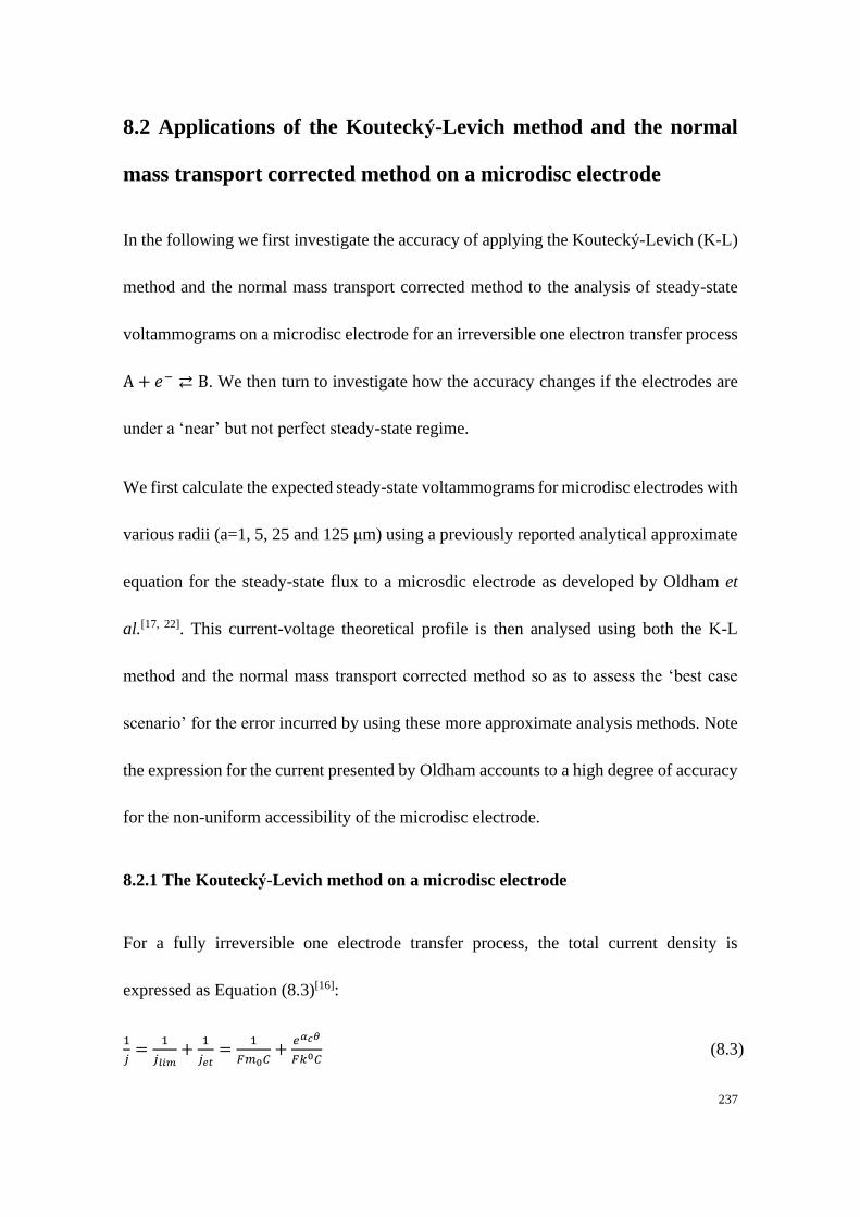
237
8.2 Applications of the Koutecky-Levich method and the normal
mass transport corrected method on a microdisc electrode
In the following we first investigate the accuracy of applying the Koutecky-Levich (K-L)
method and the normal mass transport corrected method to the analysis of steady-state
voltammograms on a microdisc electrode for an irreversible one electron transfer process
A + 𝑒− ⇄ B. We then turn to investigate how the accuracy changes if the electrodes are
under a ‘near’ but not perfect steady-state regime.
We first calculate the expected steady-state voltammograms for microdisc electrodes with
various radii (a=1, 5, 25 and 125 μm) using a previously reported analytical approximate
equation for the steady-state flux to a microsdic electrode as developed by Oldham et
al.[17, 22]. This current-voltage theoretical profile is then analysed using both the K-L
method and the normal mass transport corrected method so as to assess the ‘best case
scenario’ for the error incurred by using these more approximate analysis methods. Note
the expression for the current presented by Oldham accounts to a high degree of accuracy
for the non-uniform accessibility of the microdisc electrode.
8.2.1 The Koutecky-Levich method on a microdisc electrode
For a fully irreversible one electrode transfer process, the total current density is
expressed as Equation (8.3)[16]:
1
𝑗=
1
𝑗𝑙𝑖𝑚+
1
𝑗𝑒𝑡=
1
𝐹𝑚0𝐶+
𝑒𝛼𝑐𝜃
𝐹𝑘0𝐶 (8.3)
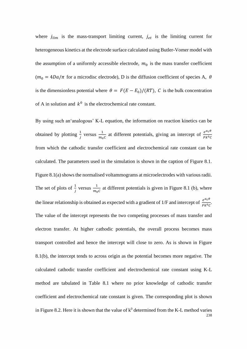
238
where 𝑗𝑙𝑖𝑚 is the mass-transport limiting current, 𝑗𝑒𝑡 is the limiting current for
heterogeneous kinetics at the electrode surface calculated using Butler-Vomer model with
the assumption of a uniformly accessible electrode, 𝑚0 is the mass transfer coefficient
(𝑚0 = 4𝐷𝑎/𝜋 for a microdisc electrode), D is the diffusion coefficient of species A, 𝜃
is the dimensionless potential where 𝜃 = 𝐹(𝐸 − 𝐸0)/(𝑅𝑇), 𝐶 is the bulk concentration
of A in solution and 𝑘0 is the electrochemical rate constant.
By using such an‘analogous’ K-L equation, the information on reaction kinetics can be
obtained by plotting 1
𝑗 versus
1
𝑚0𝐶 at different potentials, giving an intercept of
𝑒𝛼𝑐𝜃
𝐹𝑘0𝐶
from which the cathodic transfer coefficient and electrochemical rate constant can be
calculated. The parameters used in the simulation is shown in the caption of Figure 8.1.
Figure 8.1(a) shows the normalised voltammograms at microelectrodes with various radii.
The set of plots of 1
𝑗 versus
1
𝑚0𝐶 at different potentials is given in Figure 8.1 (b), where
the linear relationship is obtained as expected with a gradient of 1/F and intercept of 𝑒𝛼𝑐𝜃
𝐹𝑘0𝐶.
The value of the intercept represents the two competing processes of mass transfer and
electron transfer. At higher cathodic potentials, the overall process becomes mass
transport controlled and hence the intercept will close to zero. As is shown in Figure
8.1(b), the intercept tends to across origin as the potential becomes more negative. The
calculated cathodic transfer coefficient and electrochemical rate constant using K-L
method are tabulated in Table 8.1 where no prior knowledge of cathodic transfer
coefficient and electrochemical rate constant is given. The corresponding plot is shown
in Figure 8.2. Here it is shown that the value of k0 determined from the K-L method varies
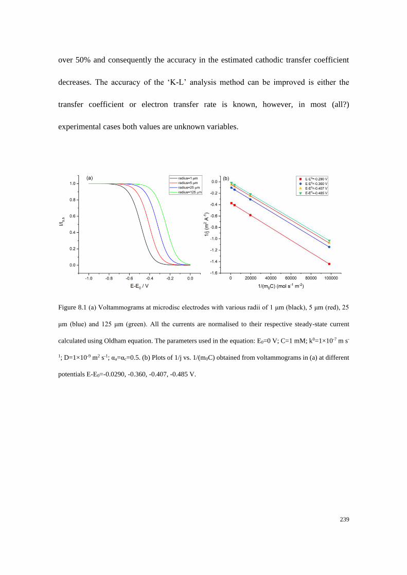
239
over 50% and consequently the accuracy in the estimated cathodic transfer coefficient
decreases. The accuracy of the ‘K-L’ analysis method can be improved is either the
transfer coefficient or electron transfer rate is known, however, in most (all?)
experimental cases both values are unknown variables.
Figure 8.1 (a) Voltammograms at microdisc electrodes with various radii of 1 μm (black), 5 μm (red), 25
μm (blue) and 125 μm (green). All the currents are normalised to their respective steady-state current
calculated using Oldham equation. The parameters used in the equation: E0=0 V; C=1 mM; k0=1×10⁻⁷ m s-
1; D=1×10⁻⁹ m2 s-1; αa=αc=0.5. (b) Plots of 1/j vs. 1/(m0C) obtained from voltammograms in (a) at different
potentials E-E0=-0.0290, -0.360, -0.407, -0.485 V.
240
Table 8.1 Calculated αc and k0 from plots in Figure 8.1(b) where αc and k0 are unknown.
Sets of
data
E-E0 / V Intercept Sets of data
used in the
calculation
αc and k0 are unknown
actual αc = 0.5, k0= 1x10⁻⁷ m s-1
αc, K-L k0 / m s-1
1) -0.29 -0.367 1) and 2) 0.4915 1.096×10⁻⁷
2) -0.36 -0.0961 1) and 3) 0.4854 1.176×10⁻⁷
3) -0.407 -0.0402 1) and 4) 0.4759 1.309×10⁻⁷
4) -0.485 -0.00989 2) and 3) 0.4761 1.360×10⁻⁷
\ \ \ 2) and 4) 0.4671 1.544×10⁻⁷
\ \ \ 3) and 4) 0.4617 1.712×10⁻⁷
Figure 8.2 Plot of calculated cathodic transfer coefficient and electrochemical rate constant calculated using
different set of data from K-L method where αa and ko are unknown.
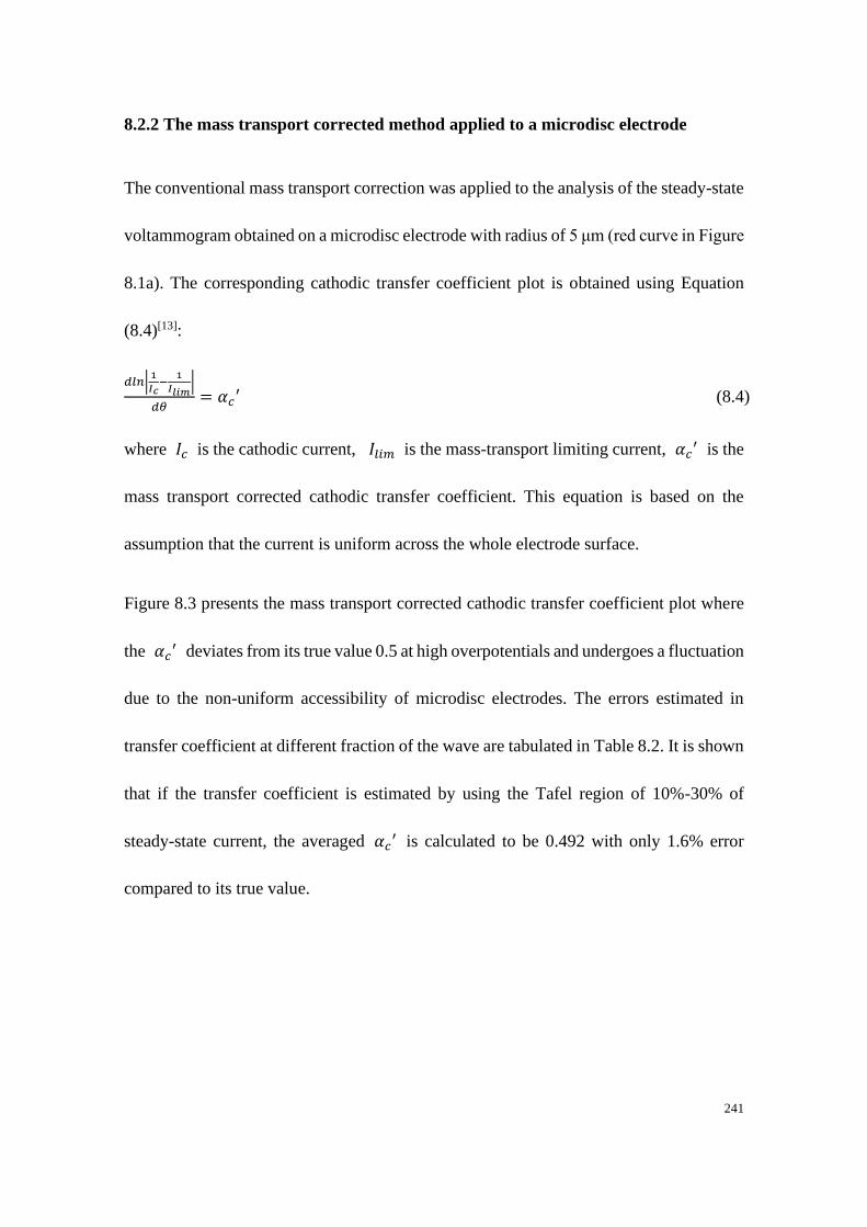
241
8.2.2 The mass transport corrected method applied to a microdisc electrode
The conventional mass transport correction was applied to the analysis of the steady-state
voltammogram obtained on a microdisc electrode with radius of 5 μm (red curve in Figure
8.1a). The corresponding cathodic transfer coefficient plot is obtained using Equation
(8.4)[13]:
𝑑𝑙𝑛|1
𝐼𝑐−
1
𝐼𝑙𝑖𝑚|
𝑑𝜃= 𝛼𝑐
′ (8.4)
where 𝐼𝑐 is the cathodic current, 𝐼𝑙𝑖𝑚 is the mass-transport limiting current, 𝛼𝑐′ is the
mass transport corrected cathodic transfer coefficient. This equation is based on the
assumption that the current is uniform across the whole electrode surface.
Figure 8.3 presents the mass transport corrected cathodic transfer coefficient plot where
the 𝛼𝑐′ deviates from its true value 0.5 at high overpotentials and undergoes a fluctuation
due to the non-uniform accessibility of microdisc electrodes. The errors estimated in
transfer coefficient at different fraction of the wave are tabulated in Table 8.2. It is shown
that if the transfer coefficient is estimated by using the Tafel region of 10%-30% of
steady-state current, the averaged 𝛼𝑐′ is calculated to be 0.492 with only 1.6% error
compared to its true value.
242
Figure 8.3 Mass transport corrected cathodic transfer coefficient on a microdisc electrode with radius of 5
μm. The black solid curve is the normalised voltammogram simulated using Oldham equation where E0=0
V; C=1 mM; k0=1×10⁻⁷ m s-1; D=1×10⁻⁹ m2 s-1; αa=αc=0.5. The dotted line stands for different fractions of
the wave (10%, 30%, 50% and 80% of Is.s). The blue solid curve is the mass transport corrected cathodic
transfer coefficient plot as a function of potential. The current range analysed is 1-99% of Is.s.
Table 8.2 Error in αc at different fraction of the voltammetric wave.
Fraction of the wave 10% of Is.s 30% 50% 80%
Error in αc <1 % 2.8% 6.0% 12%
Due to the non-uniform accessibility of microdisc electrodes, the voltammograms
obtained are often under a very ‘near’ steady state regime. Here we further investigated
how the accuracy of applying the K-L method and normal transfer coefficient changes on
microdisc electrodes under a very ‘near’ steady-state regime where the deviation from
true steady state behaviour reflects the application of a finite scan rate as opposed to an
infinitesimally slow one. The voltammograms on microdisc electrodes with various radii
243
(a=5, 10 and 20 μm) were simulated using a home-written programme by Dr Oleksiy
Klymenko based on the conformal mapping of the spatial coordinates and uses an
exponentially expanding time grid.[23] The results of using the K-L method are shown in
Figure 8.4 and Table 8.3. Figure 8.4(a) shows the normalised voltammograms at
microelectrodes with various radii. The set of plots of 1
𝑗 versus
1
𝑚0𝐶 at different
potentials is given in Figure 8.4 (b). It is shown that for a ‘near’ steady state
voltammogram, the calculated value of αc, K-L varies by 13% and the calculated value of
k0 varies by over 50% as shown in Table 8.3. The results analysed using normal mass
transport corrected method are shown in Figure 8.5 and Table 8.4. Figure 8.5 gives the
mass transport corrected cathodic transfer coefficient on a microdisc electrode with radius
of 20 μm, where the αc’ deviates from its true value at higher overpotentials. Moreover,
the behaviour of transfer coefficient as a function of potential tend to be more like the
behaviour under linear regime[13] as the radius of electrode increases. Therefore, the
results show that the accuracy in analysing a ‘near’ steady-state voltammogram decreases
for both K-L and normal mass transport corrected methods.
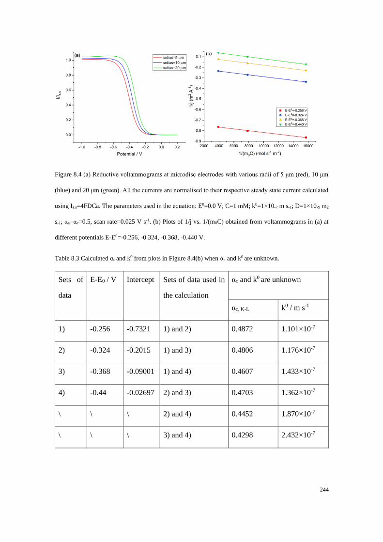
244
Figure 8.4 (a) Reductive voltammograms at microdisc electrodes with various radii of 5 μm (red), 10 μm
(blue) and 20 μm (green). All the currents are normalised to their respective steady state current calculated
using Is.s=4FDCa. The parameters used in the equation: E0=0.0 V; C=1 mM; k0=1×10⁻⁷ m s-1; D=1×10⁻⁹ m2
s-1; αa=αc=0.5, scan rate=0.025 V s-1. (b) Plots of 1/j vs. 1/(m0C) obtained from voltammograms in (a) at
different potentials E-E0=-0.256, -0.324, -0.368, -0.440 V.
Table 8.3 Calculated αc and k0 from plots in Figure 8.4(b) when αc and k0 are unknown.
Sets of
data
E-E0 / V Intercept Sets of data used in
the calculation
αc and k0 are unknown
αc, K-L k0 / m s-1
1) -0.256 -0.7321 1) and 2) 0.4872 1.101×10⁻⁷
2) -0.324 -0.2015 1) and 3) 0.4806 1.176×10⁻⁷
3) -0.368 -0.09001 1) and 4) 0.4607 1.433×10⁻⁷
4) -0.44 -0.02697 2) and 3) 0.4703 1.362×10⁻⁷
\ \ \ 2) and 4) 0.4452 1.870×10⁻⁷
\ \ \ 3) and 4) 0.4298 2.432×10⁻⁷

245
Figure 8.5 Mass transport corrected cathodic transfer coefficient on a microdisc electrode with radius of 20
μm. The black solid curve is the reductive voltammetric wave simulated normalised to its steady state
current (Is.s=4FDCa) where E0=0 V; C=1 mM; k0=1×10⁻⁷ m s-1; D=1×10⁻⁹ m2 s-1; αa=αc=0.5; scan rate=0.025
V s-1. The dotted line stands for different fractions of the wave (10%, 30%, 50% and 80% of Is.s). The blue
solid curve is the mass transport corrected cathodic transfer coefficient plot as a function of potential.
Table 8.4 Error in αc at different fraction of the voltammetric wave in Figure 8.5.
Fraction of the wave 10% of Is.s 30% 50% 80%
Error in αc 1.4% 4.6% 9.0% 26.5%
Although the K-L method and the normal mass transport corrected method have high
accuracy in the analysis of microdisc electrode under certain circumstances, neither of
them can be used as a universal analysis methodology on microdisc electrodes. Compared
to the normal mass transport corrected method and K-L method, one of the big advantages
of the extraction method in this work is that it works equally well for linear and radial
mass-transport regimes and the transition between these two limits.

246
8.3 Experimental
8.3.1 Chemical reagents
The ammonium iron (II) sulfate hexahydrate ((NH4)2FeII(SO4)2; Aldrich; 99%) and
perchloric acid (Aldrich; 70%) were used as purchased without further purification.
Solutions were freshly prepared using deionised water (Milipore) with a resistivity of 18.2
MΩ cm at a temperature of 25 oC.
8.3.2 Instrumentation
Electrochemical measurements were performed with a μAutolab Type III potentiostat
using a standard three electrode setup in an optimised thermostated electrochemical
system as described in the literature[24]. A carbon microdisc electrode (7 µm in diameter;
BASi), a saturated calomel electrode (SCE; BASi, Japan) and a platinum wire were used
as working electrode, reference electrode and counter electrode, respectively. The
working electrode was polished using alumina of decreasing size (1.0, 0.3 and 0.05 µm,
Buehler, IL), washed with deionised water and dried with nitrogen. All electrochemical
measurements were conducted at 25 oC inside a Faraday cage.
8.4 Theory
The aim of this work is to extract the electron transfer kinetics for an irreversible
electrochemical process directly from a voltammogram experimentally recorded at a
247
planar disc electrode of any size. The following theory is outlined for a reduction reaction;
however, it is equally applicable to the study of oxidative processes, as is undertaken later
in this text. The programme for this extraction was written by Dr Christopher Batchelor-
McAuley. Here we consider the one electron transfer process as given by:
A + 𝑒− ⇄ B (8.5)
where A and B are solution phase species, and initially only the reactant A is present in
solution. Furthermore, we assume that the reaction is first order with respect to the
concentration of the reactant such that the electrochemical flux at the electrode (𝑗𝐴,0)is
given by:
𝑗𝐴,0 = 𝑘𝑟𝑒𝑑𝑐𝐴,0 (8.6)
kc is the potential dependent electrochemical rate constant for the reduction of A to B and
𝑐𝐴,0 is the concentration of species A at the electrode surface (mol m-3). From this rate
constant, kred, and from the definition provide in Equation 8.1, it is possible to assess the
systems cathodic transfer coefficient (𝛼𝑐) as given by:
𝛼𝑐 = −𝑅𝑇
𝐹
𝑑 ln 𝑘𝑟𝑒𝑑
𝑑𝐸 (8.7)
In the course of the simulations we assume that the mass-transport of species in the
solution phase occurs only by diffusion and so that the system is therefore well described
by Fick’s second law. In this work we consider a planar disc electrode embedded into a

248
flat plane; consequently, for numerical efficiency[24] oblate spheroidal co-ordinates are
used.
Figure 8.6 Cross-section of the coordinate system. r and z in the figure are dimensionless where a is the
electrode radius. Y-axis is the coordinate perpendicular to the electrode surface and x-axis is the coordinate
parallel to the electrode. The vertical line at the extreme left represents the axis normal to the disc electrode
through its centre. The red and blue curves represent the uniform grid spacing in μ and ν respectively.
Equations (8.9) and (8.10) give the conversion between the spherical oblate (μ and ν) and cylindrical
coordinates (r and z).
Figure 8.6 provides a cross-section of this coordinate system. As the system is axially
symmetric then the problem can be reduced to two-dimensions and Fick’s second law
expressed as [25]:
𝜕𝑐𝐴
𝜕𝑡=
𝐷𝐴
a2(sinh2𝜇+𝑠𝑖𝑛2)(tanh𝜇
𝜕𝑐𝐴
𝜕𝜇+
𝜕2𝑐𝐴
𝜕𝜇2 − tan𝜕𝑐𝐴
𝜕+
𝜕2𝑐𝐴
𝜕2 ) (8.8)
where DA is the diffusion coefficient of species A (m2 s-1), a is the electrode radius (m), t
is the experimental time (s). Both 𝜇 and are coordinates in the oblate spheroidal
249
coordinate system and are related to the more familiar cylindrical coordinates in the 2D-
plane by:
𝑧 = 𝑎 sinh𝜇 sin (8.9)
𝑟 = 𝑎 cosh𝜇 cos (8.10)
where z is the coordinate perpendicular to the electrode surface and r is parallel to the
electrode surface. 𝜇 is a nonnegative real number and for the present case varies
between 0 and π/2. In the simulation space the electrode surface is set as where 𝜇 = 0.
Boundary conditions
To solve Equation 8.8 we need suitable boundary conditions. At the onset of the
experiment we assume the species A has a uniform concentration profile and that no B is
present in solution. The outer boundary of the simulation space is set to be sufficiently
far from the electrode to ensure that at this distance the concentrations of the electroactive
species are not altered from those of the bulk:
𝜇𝑚𝑎𝑥 = 𝑐𝑜𝑠ℎ−1(1 +6
𝑎√𝐷𝐴𝑡𝑚𝑎𝑥) (8.11)
where tmax is the duration of the experiment. The inert substrate surrounding the electrode
is defined as where = 0 and the central axis is at = 𝜋/2 . For both of these
boundaries we set a condition of zero flux. All that remains is to determine a suitable
boundary condition for the electrode surface. Usually one would assume a model for the
electron transfer kinetics and therefore simulate how the current varies as a function of

250
potential; however, here we do not assume any prior knowledge of the electrochemical
rate constant, kred. In the simulation we take a given measured current at a given potential
and on the basis of the known electrode geometry infer the reaction rate while accounting
fully for the local depletion of the reagent in the vicinity of the electrode surface. First,
taking Equation 8.6 and Fick’s first law then at the electrode interface the concentration
of the species A is described by the following:
𝑘𝑟𝑒𝑑𝑐𝐴,0 = 𝐷∇𝑐𝐴 (8.12)
where kc is an additional unknown and needs to be related to the electrochemical current
of the system. The total flux of the system is found by integration across the electrode
surface in oblate spheroidal co-ordinates this integral is:
𝐼 = 𝜋𝐹𝐷𝑎2𝑘𝑟𝑒𝑑 ∫ 𝑐𝐴,0𝜋/2
0sin (2) 𝑑 (8.13)
After discretisation the above equation provides an additional simultaneous equation to
be solved for given a knowledge of 𝐼. This set of simultaneous equations do not lead to a
simple banded matrix. To solve the problem and find kred as a function of potential it is
necessary that all of the surface concentrations which vary over the electrode surface are
considered and solved for simultaneously; consequently, the ADI method[26] is not
applicable to this problem and the equation set needs to be solved fully implicitly. Second,
the boundary condition Equations 8.12 and 8.13 are weakly non-linear. Due to this non-
linearity the system of equations were solved iteratively via the Newton-Raphson
251
method.[27] The convergence tolerance criterion required that the average absolute
magnitude of the correction term in the concentrations must be less than 1x10⁻⁸.
8.5 Numerical methods
The equation set was solved using a central finite difference method. Although the use of
a uniform grid spacing allows rapid convergence in the limit of a small (micro) electrode
simulation, for larger (macro) electrode dimension the simulation became
computationally expensive; consequently, a patching scheme was used for the grid
spacing in the μ coordinate as given by;
𝜇[𝑖] = 𝜇[𝑖 − 1] + 𝛾𝜇𝜇𝑠 𝜇 < 𝜇 s (8.14)
𝜇[𝑖] = 𝜇[𝑖 − 1] + 𝛾𝜇𝜇[𝑖 − 1] 𝜇 max> 𝜇 > 𝜇 s (8.15)
where i relates to the grid indexing. Suitable grid parameters were found to be 𝛾𝜇 =
5 × 10⁻² and 𝜇𝑠 = sinh-1(2×10⁻⁶/a). Allowing efficient simulation of the concentration
profiles in both the macro and microscopic electrode limits. The grid was uniformly
spaced in the coordinate with 400 points. As the problem is solved fully implicitly there
are no restrictions on the size of the time step used. Simulation and extraction of the
electrochemical rate constant was undertaken using a script written and run using Python
3.7, solving the sparse Jacobian matrix was achieved using spsolve function provided as
part of the SciPy package. Simulation time varies but extraction of the electrochemical
rate constant for a total of 500 time steps require 8-10 minutes of computing time on an

252
Intel Xeon E5-1620. This simulation programme is credited to Dr Christopher Batchelor-
McAuley.
8.6 Results and discussion
In the following, first a series of theoretical results are considered where the
electrochemical rate constant is ‘extracted’ from a series of numerically simulated results
predicting current-voltage curves for fully irreversible voltammograms at a microdisc
electrode. These “voltammograms” were created by a previously reported simulation
program[23] that has been extensively tested. Using these model results it is possible to
investigate the uncertainties associated with the extracted electrochemical kinetics.
Second, we use the experimental example of the oxidation of Fe2+ in aqueous solution at
a carbon micro-electrode and demonstrate how the electrochemical rate constant and
hence transfer coefficient can be directly obtained from the experimentally recorded
voltammetric response.
8.6.1 Data extraction process
Figure 8.7 depicts three simulated voltammetric profiles for a fully irreversible one
electron reduction process where the electron transfer kinetics have been simulated using
the Butler-Volmer formalism with transfer coefficients of 0.4, 0.5 and 0.6 on both
microdisc (a = 5 µm) and macroelectrode (a = 500 µm). These simulated voltammetric
profiles were then used as input for the “extraction program” and used to infer the

253
electrochemical rate constant as a function of potential from the voltammetric response.
The extraction program requires along with the (previously simulated) current voltage
profile, knowledge of the electrode radius, scan rate, analyte diffusion coefficient and
analyte concentration. From these inputs the diffusion equation (Equation 8.6) is
numerically solved to yield the concentration profile and the electrochemical rate constant
at each time step. The extraction program makes no a priori assumption regarding the
variation of the electron transfer kinetics as a function of the electrode potential. For the
three simulated voltammograms used as an input the inlay of Figure 8.7(a) depicts the
extracted electrochemical rate constant as a function of the applied potential, where the
electron transfer kinetics have been analysed up to 90% of the wave relative to the steady-
state current noting that the y axis of the inlay is on a logarithm scale. From the extracted
electrode kinetics and through the use of equation 8.5 the electrochemical transfer
coefficient can be determined. The resulting ‘extracted’ transfer coefficients are overlaid
with the original simulated voltammetry in Figure 8.7(a) and seen to be nearly constant.
The extraction simulation is able to quantitatively determine the system’s transfer
coefficient across the near entirety of the electrochemical wave. Figure 8.7(b) depicts
comparable data for a macroelectrode simulation (a = 500 µm) where the ‘extracted’
transfer coefficient only shows a small deviation from its true value in the analysed
current range up to 100% of the peak current.
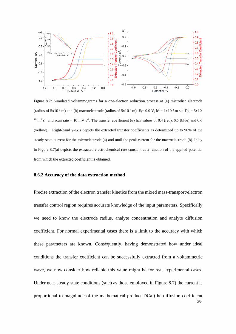
254
Figure 8.7: Simulated voltammograms for a one-electron reduction process at (a) microdisc electrode
(radius of 5x10⁻⁶ m) and (b) macroelectrode (radius of 5x10⁻⁴ m). Ef= 0.0 V, k0 = 1x10⁻⁸ m s-1, DA = 5x10-
10 m2 s-1 and scan rate = 10 mV s-1. The transfer coefficient (α) has values of 0.4 (red), 0.5 (blue) and 0.6
(yellow). Right-hand y-axis depicts the extracted transfer coefficients as determined up to 90% of the
steady-state current for the microelectrode (a) and until the peak current for the macroelectrode (b). Inlay
in Figure 8.7(a) depicts the extracted electrochemical rate constant as a function of the applied potential
from which the extracted coefficient is obtained.
8.6.2 Accuracy of the data extraction method
Precise extraction of the electron transfer kinetics from the mixed mass-transport/electron
transfer control region requires accurate knowledge of the input parameters. Specifically
we need to know the electrode radius, analyte concentration and analyte diffusion
coefficient. For normal experimental cases there is a limit to the accuracy with which
these parameters are known. Consequently, having demonstrated how under ideal
conditions the transfer coefficient can be successfully extracted from a voltammetric
wave, we now consider how reliable this value might be for real experimental cases.
Under near-steady-state conditions (such as those employed in Figure 8.7) the current is
proportional to magnitude of the mathematical product DCa (the diffusion coefficient
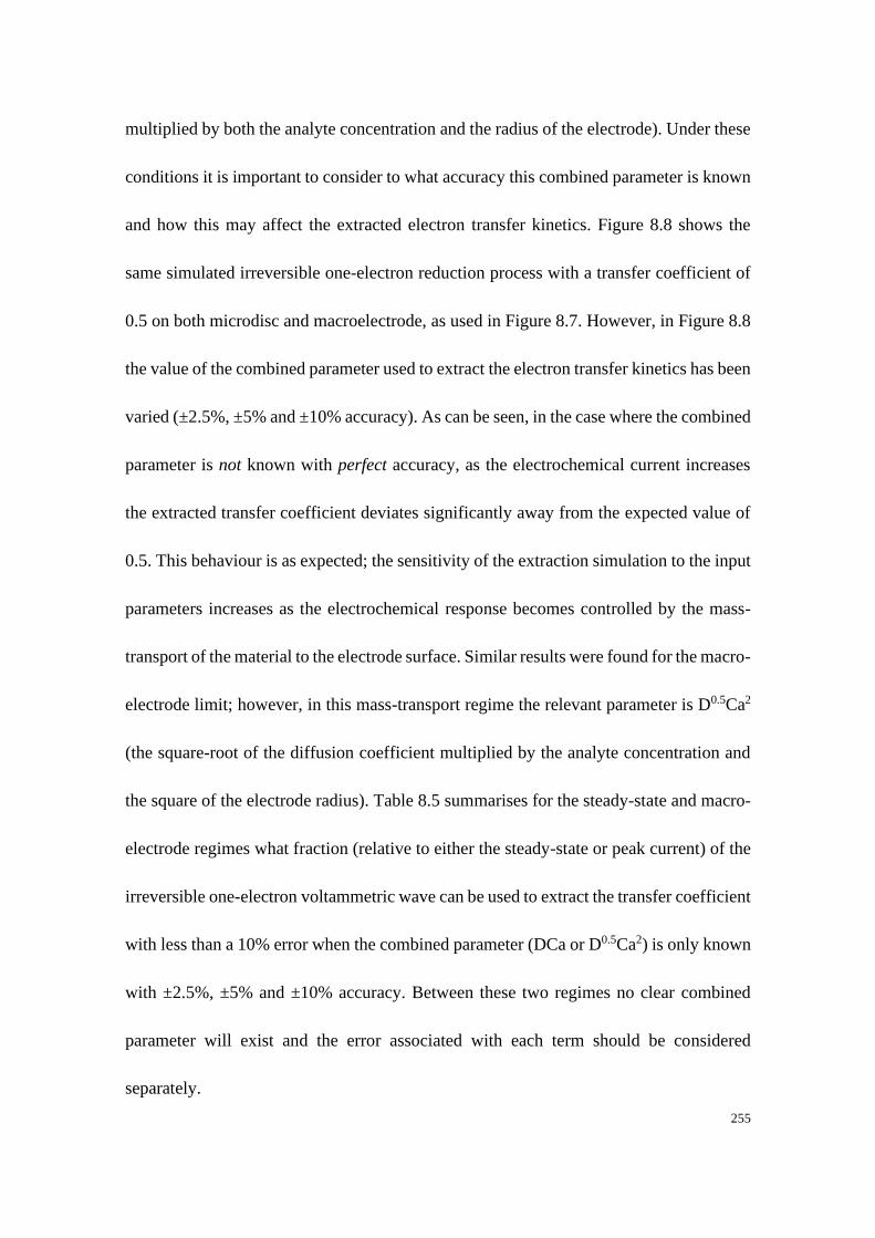
255
multiplied by both the analyte concentration and the radius of the electrode). Under these
conditions it is important to consider to what accuracy this combined parameter is known
and how this may affect the extracted electron transfer kinetics. Figure 8.8 shows the
same simulated irreversible one-electron reduction process with a transfer coefficient of
0.5 on both microdisc and macroelectrode, as used in Figure 8.7. However, in Figure 8.8
the value of the combined parameter used to extract the electron transfer kinetics has been
varied (±2.5%, ±5% and ±10% accuracy). As can be seen, in the case where the combined
parameter is not known with perfect accuracy, as the electrochemical current increases
the extracted transfer coefficient deviates significantly away from the expected value of
0.5. This behaviour is as expected; the sensitivity of the extraction simulation to the input
parameters increases as the electrochemical response becomes controlled by the mass-
transport of the material to the electrode surface. Similar results were found for the macro-
electrode limit; however, in this mass-transport regime the relevant parameter is D0.5Ca2
(the square-root of the diffusion coefficient multiplied by the analyte concentration and
the square of the electrode radius). Table 8.5 summarises for the steady-state and macro-
electrode regimes what fraction (relative to either the steady-state or peak current) of the
irreversible one-electron voltammetric wave can be used to extract the transfer coefficient
with less than a 10% error when the combined parameter (DCa or D0.5Ca2) is only known
with ±2.5%, ±5% and ±10% accuracy. Between these two regimes no clear combined
parameter will exist and the error associated with each term should be considered
separately.
256
Figure 8.8 Variation and uncertainty in the extract transfer coefficient for (a) a steady-state voltammetric
response from a microdisc electrode and (b) a peak-shaped voltammetric response from a macroelectrode
with a constant transfer coefficient of 0.5. For the extraction of the electron transfer coefficient the
combined parameter DCa (microelectrode) and D0.5Ca2 (macroelectrode, see text) has been varied by ±2.5%
(green), ±5% (blue) and ±10% (red). At higher current densities and as the voltammetric reaction rate
becomes controlled by the mass-transport of material to the electrode surface the extracted transfer
coefficient deviates significantly away from the actual value of 0.5.
Table 8.5: Fraction of the voltammetric wave (relative to the steady-state or peak current) that can be
analysed to extract the transfer coefficient with less than 10% error when the combined parameter DCa
(microelectrode) or D0.5Ca2 (macroelectrode) is only known to an accuracy of ±2.5%, ±5% and ±10%.
±2.5% ±5% ±10%
Microelectrode
DCa
0.78 0.61 0.44
Macroelectrode
D0.5Ca2
0.99 0.93 0.73
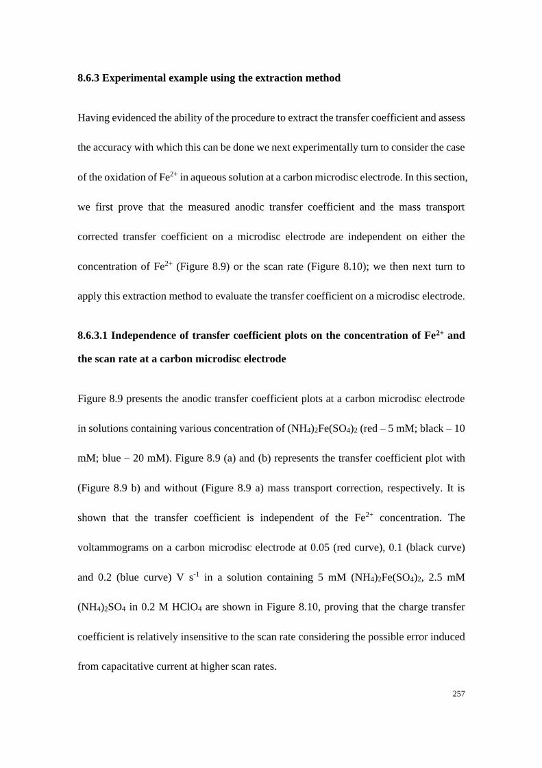
257
8.6.3 Experimental example using the extraction method
Having evidenced the ability of the procedure to extract the transfer coefficient and assess
the accuracy with which this can be done we next experimentally turn to consider the case
of the oxidation of Fe2+ in aqueous solution at a carbon microdisc electrode. In this section,
we first prove that the measured anodic transfer coefficient and the mass transport
corrected transfer coefficient on a microdisc electrode are independent on either the
concentration of Fe2+ (Figure 8.9) or the scan rate (Figure 8.10); we then next turn to
apply this extraction method to evaluate the transfer coefficient on a microdisc electrode.
8.6.3.1 Independence of transfer coefficient plots on the concentration of Fe2+ and
the scan rate at a carbon microdisc electrode
Figure 8.9 presents the anodic transfer coefficient plots at a carbon microdisc electrode
in solutions containing various concentration of (NH4)2Fe(SO4)2 (red – 5 mM; black – 10
mM; blue – 20 mM). Figure 8.9 (a) and (b) represents the transfer coefficient plot with
(Figure 8.9 b) and without (Figure 8.9 a) mass transport correction, respectively. It is
shown that the transfer coefficient is independent of the Fe2+ concentration. The
voltammograms on a carbon microdisc electrode at 0.05 (red curve), 0.1 (black curve)
and 0.2 (blue curve) V s-1 in a solution containing 5 mM (NH4)2Fe(SO4)2, 2.5 mM
(NH4)2SO4 in 0.2 M HClO4 are shown in Figure 8.10, proving that the charge transfer
coefficient is relatively insensitive to the scan rate considering the possible error induced
from capacitative current at higher scan rates.
258
Figure 8.9 Anodic transfer coefficient plot as a function of concentration of Fe2+ (red – 5mM; black – 10
mM; blue – 20 mM) without (a) and with (b) mass transport correction. Solution composition:
(NH4)2Fe(SO4)2, 2.5 mM (NH4)2SO4 in 0.2 M HClO4. Analysis was done with background subtraction.
Figure 8.10 Anodic transfer coefficient plot as a function of scan rate (red – 0.05 V s-1; black – 0.1 V s-1;
blue – 0.2 V s-1) without (a) and with (b) mass transport correction. Solution composition: (NH4)2Fe(SO4)2,
2.5 mM (NH4)2SO4 in 0.2 M HClO4. Analysis was done with background subtraction.
8.6.3.2 Experimental example of the extraction applied to a microdisc electrode
In Figure 8.11 the background current associated with the capacitative charging which
was measured in blank solution without Fe2+/3+ redox couple in the same potential window
has been subtracted and removed. There are two notable features regarding this

259
voltammetric response, first as the formal potential for this redox couple is 0.4785 (±
0.0006) V vs. SCE then the main oxidation process occurs at a high overpotential.[28]
Second, at low over potentials a significant pre-wave is observable. The origin of this pre-
wave has recently been extensively investigated and shown to be due to a surface specific
catalytic mechanism.[28] Overlaid on the experimental voltammetric response is the
extracted transfer coefficient for the system where the uncertainty of this extracted value
has been accounted for by considering the accuracy to which the input parameters are
known. The diffusion coefficient for Fe2+ under these conditions has been determined to
be 6.68 (± 0.14) × 10-10 m2 s-1. Further the electrode has been previously calibrated and
found to have a radius of 3.64 µm.[28] We consider that this radius is accurate within 2%
and that the uncertainty in the bulk concentration of Fe2+ is essentially negligible. From
Figure 8.11 it can be seen that across the full potential range the transfer coefficient is
significantly below 0.5. At low overpotentials (around + 0.55 V vs SCE) the transfer
coefficient goes through a minimum, this is due to the oxidative pre-wave where the rate
of electron transfer becomes relatively insensitive to changes in the applied potential.
Again at higher potentials the transfer coefficient increases but to a value in the region of
~0.3. In this case the variable transfer coefficient directly reflects the change in the
electrochemical mechanism of the oxidation of solution phase Fe(II) as a function of the
applied potential. Due to the presence of the pre-wave at potentials that would commonly
be used for Tafel analysis determination of the electrochemical transfer coefficient for the
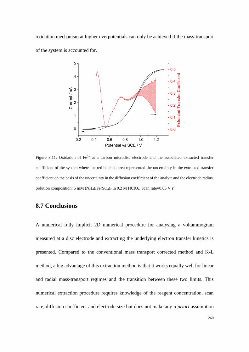
260
oxidation mechanism at higher overpotentials can only be achieved if the mass-transport
of the system is accounted for.
Figure 8.11: Oxidation of Fe2+ at a carbon microdisc electrode and the associated extracted transfer
coefficient of the system where the red hatched area represented the uncertainty in the extracted transfer
coefficient on the basis of the uncertainty in the diffusion coefficient of the analyte and the electrode radius.
Solution composition: 5 mM (NH4)2Fe(SO4)2 in 0.2 M HClO4. Scan rate=0.05 V s-1.
8.7 Conclusions
A numerical fully implicit 2D numerical procedure for analysing a voltammogram
measured at a disc electrode and extracting the underlying electron transfer kinetics is
presented. Compared to the conventional mass transport corrected method and K-L
method, a big advantage of this extraction method is that it works equally well for linear
and radial mass-transport regimes and the transition between these two limits. This
numerical extraction procedure requires knowledge of the reagent concentration, scan
rate, diffusion coefficient and electrode size but does not make any a priori assumption
261
regarding the sensitivity of the electrode kinetics to the applied electrode potential.
Changes in the surface concentration of the reagent is accounted for by solving the 2D
diffusion equation and numerically simulating to find the concentration profile in the
vicinity of the electrode and therefore inferring the surface concentrations during the
course of the voltammetric experiment, where the concentrations vary across the
electrode surface. The accuracy of this extraction process is predicated on precise
knowledge of the physical parameters defining the system, most importantly the diffusion
coefficient, analyte concentration and electrode radius need to be known as accurately as
possible. Assuming that the combination of these physical parameters is known to with
±2.5% accuracy then for a microdisc electrode 78% of the voltammetric wave can be
analysed and the resulting transfer coefficient will be within 10% of the actual value.
Similarly, for a macro-disc system up to 99% of the peak current can be used to determine
the electrochemical systems transfer coefficient. Hypothetically, with the diffusion
coefficient, electrode dimensions and analyte concentration known to arbitrary accuracy
then in principle the proposed numerical extraction procedure could allow in all case >
99% of the voltammetric wave to be analysed to yield an accurate measure of the transfer
coefficient.
References:
[1] R. Guidelli, R. G. Compton, J. M. Feliu, E. Gileadi, J. Lipkowski, W. Schmickler, S. Trasatti, Pure
and Applied Chemistry 2014, 86, 245-258.
[2] R. Guidelli, R. G. Compton, J. M. Feliu, E. Gileadi, J. Lipkowski, W. Schmickler, S. Trasatti, Pure
and Applied Chemistry 2014, 86, 259-262.
262
[3] R. G. Compton, E. L. Laborda, K. R. Ward, Understanding Voltammetry: Simulation Of Electrode
Processes, World Scientific Publishing Company, 2013.
[4] E. Gileadi, Journal of Solid State Electrochemistry 2011, 15, 1359.
[5] C. E. D. Chidsey, Science 1991, 251, 919-922.
[6] S. W. Feldberg, Analytical Chemistry 2010, 82, 5176-5183.
[7] V. Mirceski, E. Laborda, D. Guziejewski, R. G. Compton, Analytical Chemistry 2013, 85, 5586-
5594.
[8] E. Laborda, M. C. Henstridge, C. Batchelor-McAuley, R. G. Compton, Chemical Society Reviews
2013, 42, 4894-4905.
[9] C. Batchelor-McAuley, R. G. Compton, Journal of Electroanalytical Chemistry 2012, 669, 73-81.
[10] S. Fletcher, Journal of Solid State Electrochemistry 2009, 13, 537-549.
[11] aJ. M. Savéant, D. Tessier, Journal of Electroanalytical Chemistry and Interfacial
Electrochemistry 1975, 65, 57-66; bJ.-M. Savéant, D. Tessier, Faraday Discussions of the
Chemical Society 1982, 74, 57-72; cJ. M. Saveant, D. Tessier, The Journal of Physical Chemistry
1977, 81, 2192-2197.
[12] aH. O. Finklea, The Journal of Physical Chemistry B 2001, 105, 8685-8693; bH. O. Finklea,
Journal of Electroanalytical Chemistry 2001, 495, 79-86.
[13] D. Li, C. Lin, C. Batchelor-McAuley, L. Chen, R. G. Compton, Journal of Electroanalytical
Chemistry 2018, 826, 117-124.
[14] D. Li, C. Batchelor-McAuley, R. G. Compton, Applied Materials Today 2019.
[15] aW. J. Albery, Electrode kinetics, Vol. 14, Oxford University Press, 1975; bK. J. J. Mayrhofer, D.
Strmcnik, B. B. Blizanac, V. Stamenkovic, M. Arenz, N. M. Markovic, Electrochimica Acta 2008,
53, 3181-3188.
[16] J. Kim, A. J. Bard, Analytical Chemistry 2016, 88, 1742-1747.
[17] A. Molina, J. Gonzalez, E. O. Barnes, R. G. Compton, The Journal of Physical Chemistry C 2014,
118, 346-356.
[18] Q. Chen, L. Luo, Langmuir 2018, 34, 4554-4559.
[19] M. C. Henstridge, R. G. Compton, Journal of Electroanalytical Chemistry 2012, 681, 109-112.
[20] C. G. Zoski, K. B. Oldham, P. J. Mahon, T. L. E. Henderson, A. M. Bond, Journal of
electroanalytical chemistry and interfacial electrochemistry 1991, 297, 1-17.
[21] P. J. Mahon, K. B. Oldham, Electrochimica acta 2001, 46, 953-965.
[22] K. B. Oldham, C. G. Zoski, Journal of Electroanalytical Chemistry and Interfacial
Electrochemistry 1991, 313, 17-28.
[23] O. V. Klymenko, R. G. Evans, C. Hardacre, I. B. Svir, R. G. Compton, Journal of
Electroanalytical Chemistry 2004, 571, 211-221.
[24] aA. C. Michael, R. M. Wightman, C. A. Amatore, Journal of Electroanalytical Chemistry and
Interfacial Electrochemistry 1989, 267, 33-45; bA. Oleinick, C. Amatore, I. Svir, Electrochemistry
Communications 2004, 6, 588-594.
[25] aJ. C. Myland, K. B. Oldham, Journal of Electroanalytical Chemistry 2005, 576, 353-362; bP.
Moon, D. E. Spencer, Field Theory Handbook: Including Coordinate Systems, Differential
Equations and Their Solutions, Springer Berlin Heidelberg, 2012.

263
[26] J. Heinze, Journal of Electroanalytical Chemistry and Interfacial Electrochemistry 1981, 124, 73-
86.
[27] aE. Ziegel, Taylor & Francis Group, 1987; bE. J. F. Dickinson, J. G. Limon-Petersen, N. V. Rees,
R. G. Compton, The Journal of Physical Chemistry C 2009, 113, 11157-11171.
[28] D. Li, C. Batchelor-McAuley, L. Chen, R. G. Compton, The Journal of Physical Chemistry Letters
2020, 11, 1497-1501.
264
Chapter 9
Overall Conclusions
Tafel analysis is a key component of the electrochemists’ tool box for the study of
electrode kinetics. This thesis has investigated how Tafel analysis can be employed to
improve the insights gleaned in interpreting kinetic information from heterogeneous
electron transfer processes.
In voltammetric measurements where the voltammograms are generally analysed on the
basis of diffusion-controlled processes, the control of temperature of the system is
therefore vital to eliminate the change in mass transport due to natural convection induced
by the changes in solution temperature. The work presented in this thesis first proves that
imperfect thermostating system can lead to the presence of bulk convective flow the
velocity of which is experimentally shown to be of the order of 100 μm s-1 and therefore
significantly influences the voltammetric response. It is suggested that an electrochemical
cell which is closed to the environment should be employed to minimise convective flows
induced by evaporative loss of the solution. Importantly it is also shown that for
microelectrodes where the electrode material is inlaid into a large macroscopic insulating
surface the observed voltammetry is less sensitive to the solution phase convection. Such
studies provide the basis for the further kinetics study based on the voltammograms
265
obtained in electrochemical systems in which the effect of natural convection is
minimised.
Tafel analysis of a voltammogram yields a measure of the electrochemical system’s
transfer coefficient which provides information on electrochemical mechanisms. The
appropriate Tafel region used in Tafel analysis under different electrode geometries and
if and how the measurement of transfer coefficient can be improved by mass transport
correction were investigated theoretically. It is proved that the analytical mass transport
correction using a plot of ln |1
𝐼−
1
𝐼𝑙𝑖𝑚| against potential is only applicable to
microelectrodes under a true steady-state regime (i.e. micro-(hemi)spherical electrodes).
For electrodes under quasi-steady state regimes, the fraction of the voltammetric wave
used in Tafel analysis can be improved to 48.3% (micro-hemicylinder) and 77.6% (single
microband) with less than 10% error in the measured transfer coefficient after this
analytical mass transport correction. For macroelectrodes under a linear diffusion regime,
a new empirical mass-transport correction is suggested to improve the estimation of the
transfer coefficient.
Furthermore, such analytical mass transport correction is found to give significant error
in the transfer coefficient on a microdisc electrode due to its non-uniform accessibility. A
simple simulation method is developed to extract the electrochemcial kinetics based on
the knowledge of the values of the diffusion coefficient, analyte concentration and
electrode radius which need to be known as accurately as possible. Most importantly this
266
extraction process is applicable for both linear and radial mass-transport regimes.
Assuming that the diffusion coefficient, electrode dimensions and analyte concentration
are known to arbitrary accuracy then in principle the proposed numerical extraction
procedure could allow in all cases > 99% of the voltammetric wave to be analysed to
yield an accurate measure of the transfer coefficient.
Tafel analysis has been widely employed to evaluate the activity of electrocatalysts. In
this thesis, we discuss how Tafel analysis can be applied and interpretated to accurately
report the electrocatalytic performance of nanomaterials. We suggest that it is preferable
to define a current range relative to the limiting steady state value as opposed to defining
a suitable potential range for meaningful Tafel analysis giving either a transfer coefficient
or, equivalently, a ‘Tafel slope’. In addition, a suitable background subtraction of the
voltammogram needs to be first applied to eliminate the error in kinetic analysis caused
by the existence of capacitative current of the electrode.
Such theoretical results on Tafel anlysis are further employed in characterising band
electrodes with unknown dimensions using a fully irreversible redox couple without prior
knowledge of the electron transfer rate constant or the formal potential. By using the peak-
to-peak separation (Ep-p) and the magnitude of the ratio of backward peak current to
forward peak current (|Ibackward/Iforward|) as diagnostic parameters, the band width can be
estimated within 4% of its true value and with an error in length of less than 1%.
267
Finally, based on the results of Tafel analysis, the Fe2+/3+ redox reaction is proved to be
mediated via intrinsic surface quinones on carbon substrates with the evidence of a
potential dependent transfer coefficient from experimentally obtaiend voltammograms.
To summarise, this thesis has presented the investigations on how Tafel analysis can be
employed under different electrode geometries to accurately interpretate the kinetic
information of electrode processes. The capacitative current should be removed from the
experimental voltammogram using a suitable background subtraction prior to further
analysis. Proper mass-transport corrected Tafel analysis is then suggested to improve the
accuracy of the estimation of the transfer coefficient.
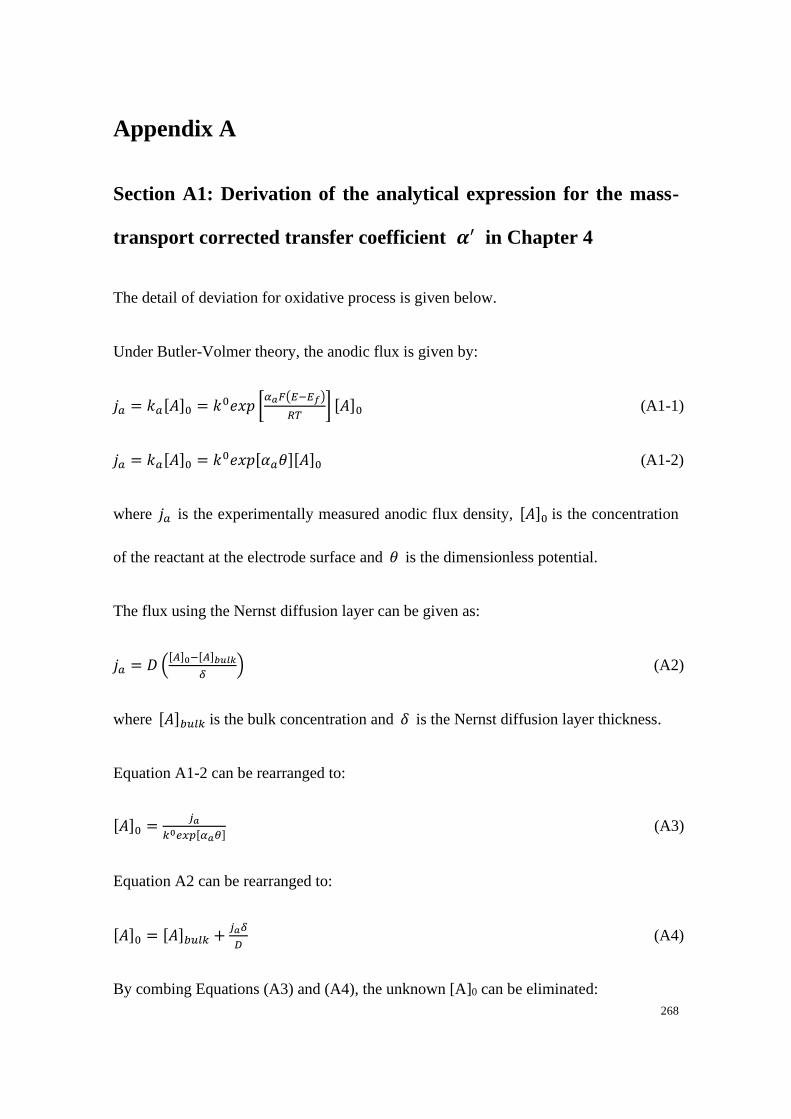
268
Appendix A
Section A1: Derivation of the analytical expression for the mass-
transport corrected transfer coefficient 𝜶′ in Chapter 4
The detail of deviation for oxidative process is given below.
Under Butler-Volmer theory, the anodic flux is given by:
𝑗𝑎 = 𝑘𝑎[𝐴]0 = 𝑘0𝑒𝑥𝑝 [𝛼𝑎𝐹(𝐸−𝐸𝑓)
𝑅𝑇] [𝐴]0 (A1-1)
𝑗𝑎 = 𝑘𝑎[𝐴]0 = 𝑘0𝑒𝑥𝑝[𝛼𝑎𝜃][𝐴]0 (A1-2)
where 𝑗𝑎 is the experimentally measured anodic flux density, [𝐴]0 is the concentration
of the reactant at the electrode surface and 𝜃 is the dimensionless potential.
The flux using the Nernst diffusion layer can be given as:
𝑗𝑎 = 𝐷 ([𝐴]0−[𝐴]𝑏𝑢𝑙𝑘
𝛿) (A2)
where [𝐴]𝑏𝑢𝑙𝑘 is the bulk concentration and 𝛿 is the Nernst diffusion layer thickness.
Equation A1-2 can be rearranged to:
[𝐴]0 =𝑗𝑎
𝑘0𝑒𝑥𝑝[𝛼𝑎𝜃] (A3)
Equation A2 can be rearranged to:
[𝐴]0 = [𝐴]𝑏𝑢𝑙𝑘 +𝑗𝑎𝛿
𝐷 (A4)
By combing Equations (A3) and (A4), the unknown [A]0 can be eliminated:
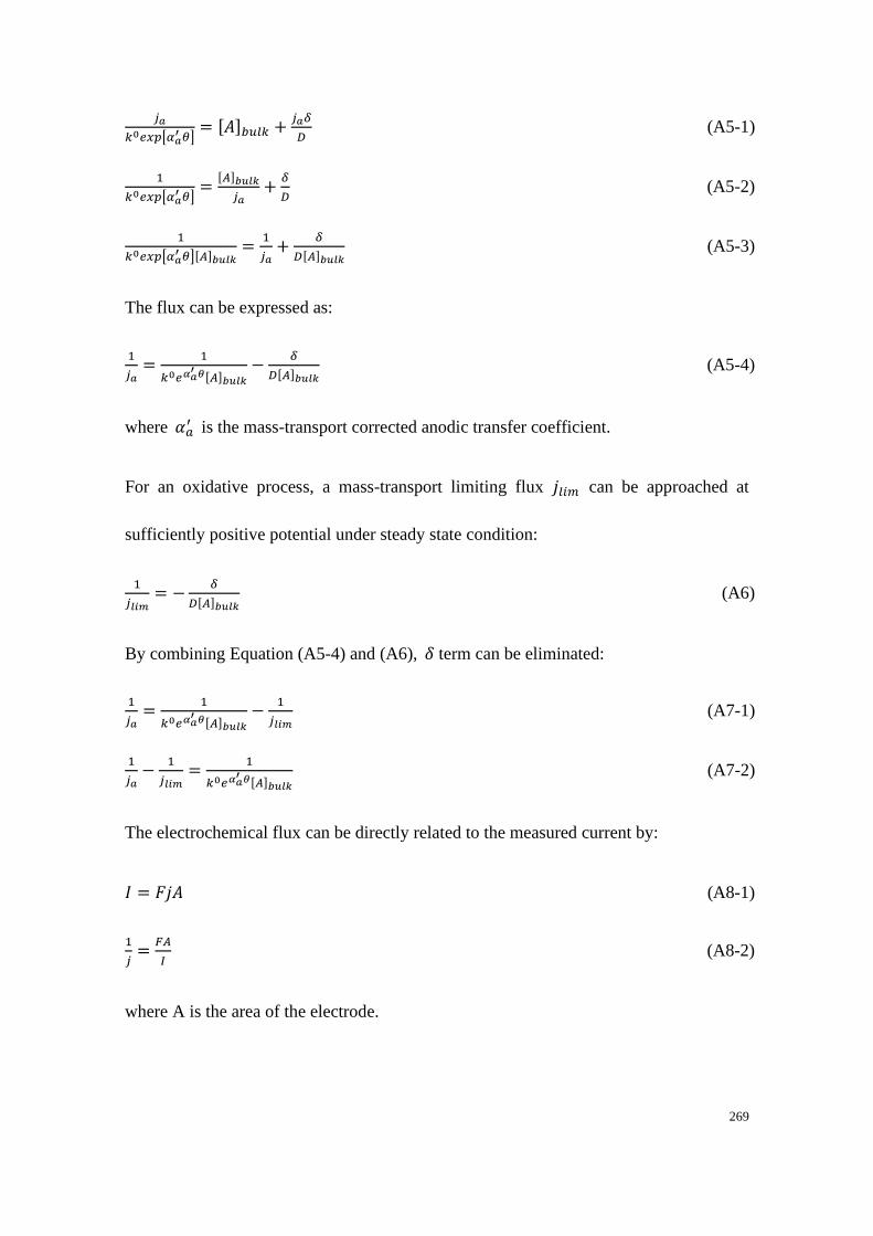
269
𝑗𝑎
𝑘0𝑒𝑥𝑝[𝛼𝑎′ 𝜃]
= [𝐴]𝑏𝑢𝑙𝑘 +𝑗𝑎𝛿
𝐷 (A5-1)
1
𝑘0𝑒𝑥𝑝[𝛼𝑎′ 𝜃]
=[𝐴]𝑏𝑢𝑙𝑘
𝑗𝑎+
𝛿
𝐷 (A5-2)
1
𝑘0𝑒𝑥𝑝[𝛼𝑎′ 𝜃][𝐴]𝑏𝑢𝑙𝑘
=1
𝑗𝑎+
𝛿
𝐷[𝐴]𝑏𝑢𝑙𝑘 (A5-3)
The flux can be expressed as:
1
𝑗𝑎=
1
𝑘0𝑒𝛼𝑎′ 𝜃[𝐴]𝑏𝑢𝑙𝑘
−𝛿
𝐷[𝐴]𝑏𝑢𝑙𝑘 (A5-4)
where 𝛼𝑎′ is the mass-transport corrected anodic transfer coefficient.
For an oxidative process, a mass-transport limiting flux 𝑗𝑙𝑖𝑚 can be approached at
sufficiently positive potential under steady state condition:
1
𝑗𝑙𝑖𝑚= −
𝛿
𝐷[𝐴]𝑏𝑢𝑙𝑘 (A6)
By combining Equation (A5-4) and (A6), 𝛿 term can be eliminated:
1
𝑗𝑎=
1
𝑘0𝑒𝛼𝑎′ 𝜃[𝐴]𝑏𝑢𝑙𝑘
−1
𝑗𝑙𝑖𝑚 (A7-1)
1
𝑗𝑎−
1
𝑗𝑙𝑖𝑚=
1
𝑘0𝑒𝛼𝑎′ 𝜃[𝐴]𝑏𝑢𝑙𝑘
(A7-2)
The electrochemical flux can be directly related to the measured current by:
𝐼 = 𝐹𝑗𝐴 (A8-1)
1
𝑗=
𝐹𝐴
𝐼 (A8-2)
where A is the area of the electrode.
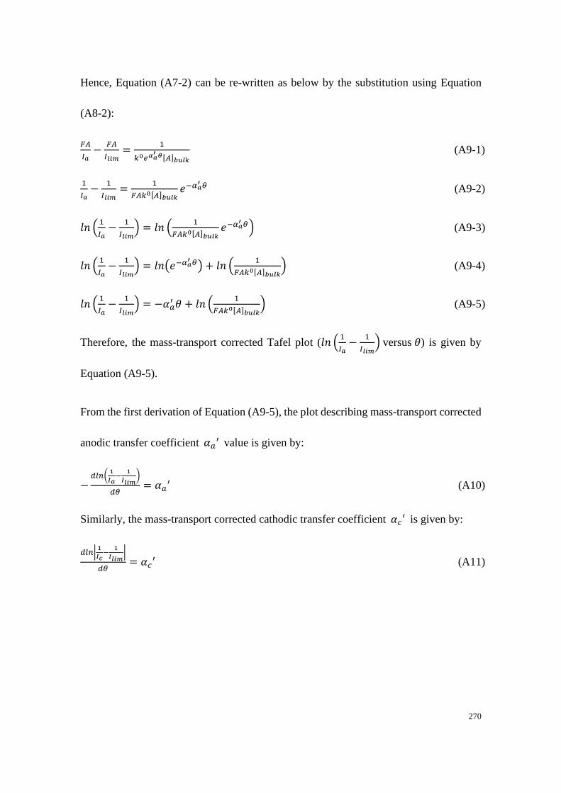
270
Hence, Equation (A7-2) can be re-written as below by the substitution using Equation
(A8-2):
𝐹𝐴
𝐼𝑎−
𝐹𝐴
𝐼𝑙𝑖𝑚=
1
𝑘0𝑒𝛼𝑎′ 𝜃[𝐴]𝑏𝑢𝑙𝑘
(A9-1)
1
𝐼𝑎−
1
𝐼𝑙𝑖𝑚=
1
𝐹𝐴𝑘0[𝐴]𝑏𝑢𝑙𝑘𝑒−𝛼𝑎
′ 𝜃 (A9-2)
𝑙𝑛 (1
𝐼𝑎−
1
𝐼𝑙𝑖𝑚) = 𝑙𝑛 (
1
𝐹𝐴𝑘0[𝐴]𝑏𝑢𝑙𝑘𝑒−𝛼𝑎
′ 𝜃) (A9-3)
𝑙𝑛 (1
𝐼𝑎−
1
𝐼𝑙𝑖𝑚) = 𝑙𝑛(𝑒−𝛼𝑎
′ 𝜃) + 𝑙𝑛 (1
𝐹𝐴𝑘0[𝐴]𝑏𝑢𝑙𝑘) (A9-4)
𝑙𝑛 (1
𝐼𝑎−
1
𝐼𝑙𝑖𝑚) = −𝛼𝑎
′ 𝜃 + 𝑙𝑛 (1
𝐹𝐴𝑘0[𝐴]𝑏𝑢𝑙𝑘) (A9-5)
Therefore, the mass-transport corrected Tafel plot (𝑙𝑛 (1
𝐼𝑎−
1
𝐼𝑙𝑖𝑚) versus 𝜃) is given by
Equation (A9-5).
From the first derivation of Equation (A9-5), the plot describing mass-transport corrected
anodic transfer coefficient 𝛼𝑎′ value is given by:
−𝑑𝑙𝑛(
1
𝐼𝑎−
1
𝐼𝑙𝑖𝑚)
𝑑𝜃= 𝛼𝑎
′ (A10)
Similarly, the mass-transport corrected cathodic transfer coefficient 𝛼𝑐′ is given by:
𝑑𝑙𝑛|1
𝐼𝑐−
1
𝐼𝑙𝑖𝑚|
𝑑𝜃= 𝛼𝑐
′ (A11)

271
Section A2: Establishing the lower current limit on different
electrodes in Chapter 4
The charge transfer in a reaction is either faradaic or capacitive. The total current is
therefore assumed to be composed of the faradaic current 𝐼𝑓 and a capacitive current 𝐼𝑐
(i.e. 𝐼𝑡𝑜𝑡 = 𝐼𝑓 + 𝐼𝑐 ). The current region chosen in the Tafel analysis should avoid the
influence from background current, where the ratio of 𝐼𝑓 to 𝐼𝑐 should be larger than 10.
For both macroelectrodes and microelectrodes, the 𝐼𝑐 is proportional to the electroactive
area of the electrode. However, 𝐼𝑓,𝑚𝑎𝑐 varies linearly with the area of the macroelectrode,
whereas 𝐼𝑓,𝑚𝑖𝑐 varies linearly with the radius of the microelectrode[1]. Therefore, the
lower limit should be different for different electrodes. Examples of a microelectrode and
macroelectrode are given below.
We consider an irreversible one-electron transfer process on a macroelectrode and assume
the radius of the electrode 𝑟𝑒𝑙 is 1 mm, the bulk concentration of reactant [𝐴]𝑏𝑢𝑙𝑘 is 1
mM, the diffusion coefficient of reactant D is 1 × 10⁻⁹ m2 s-1, the anodic transfer
coefficient 𝛼𝑎is 0.5 and the scan rate ν is 0.025 V s-1. At the electrode-solution interface,
the double-layer capacitance C is typically in the range of 10 to 40 μF cm-2 at a given
potential[2]. A specific apparent capacitance (Farads per unit geometric area) of 20 μF cm-
2 is assumed in the calculation.
The peak current on a macroelectrode is:
𝐼𝑝𝑒𝑎𝑘 = 2.99 × 10⁵𝐴𝐷1/2𝜈1/2𝛼𝑎1/2[𝐴]𝑏𝑢𝑙𝑘 = 3.32 × 10⁻⁶ 𝐴

272
The capacitive current[3] is:
𝐼𝑐,𝑚𝑎𝑐 = 𝐶 × 𝐴 × 𝜈 = 1.57 × 10⁻⁸ 𝐴
If the lower limit is chosen when the ratio of 𝐼𝑓 to 𝐼𝑐 is larger than 10, the lower
percentage of the current is given by:
𝐿𝑜𝑤𝑒𝑟 𝑝𝑒𝑟𝑐𝑒𝑛𝑡𝑎𝑔𝑒 𝑜𝑓 𝑡ℎ𝑒 𝑐𝑢𝑟𝑟𝑒𝑛𝑡 ≥10 × 𝐼𝑐,𝑚𝑎𝑐
𝐼𝑝𝑒𝑎𝑘= 4.7%
In the case of a microdisc electrode with a radius 𝑟𝑒𝑙 of 10 μm, which is 100 times smaller
than that of the macroelectrode, the steady-state current is then calculated as:
𝐼𝑠.𝑠 = 4𝐹𝐷[𝐴]𝑏𝑢𝑙𝑘𝑟𝑒𝑙 = 3.86 × 10⁻⁹ 𝐴
The capacitive current is: 𝐼𝑐,𝑚𝑖𝑐 = 𝐶 × 𝐴 × 𝜈 = 1.57 × 10⁻¹² 𝐴
Hence, 𝐿𝑜𝑤𝑒𝑟 𝑝𝑒𝑟𝑐𝑒𝑛𝑡𝑎𝑔𝑒 𝑜𝑓 𝑡ℎ𝑒 𝑐𝑢𝑟𝑟𝑒𝑛𝑡 ≥10×𝐼𝑐,𝑚𝑖𝑐
𝐼𝑠.𝑠= 0.41%
From the calculation, theoretically a lower current limit in Tafel analysis can be chosen
on a microelectrode that on a macroelectrode. In reality, the capacitance is normally much
larger, which may be due to the larger electroactive area of the electrode compared to its
geometric area, poor sealing and the stray capacitance at the electrode etc[4]. This leads to
an increase in the background current, and the lower percentage limit can become
hundreds of times larger than the theoretical value. Therefore, the lower limit of 1% for
Tafel analysis is used in this paper to analyse the whole current region. However, care
must be taken for the lower current limit in real situations.
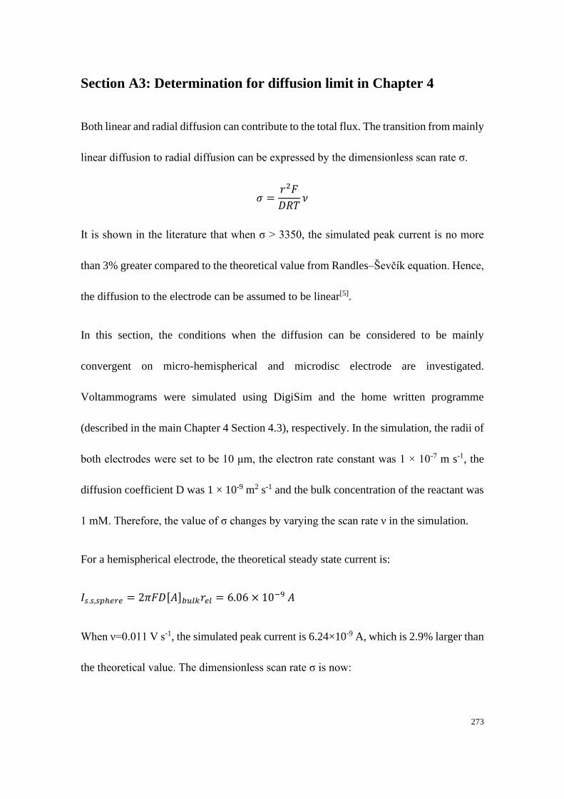
273
Section A3: Determination for diffusion limit in Chapter 4
Both linear and radial diffusion can contribute to the total flux. The transition from mainly
linear diffusion to radial diffusion can be expressed by the dimensionless scan rate σ.
𝜎 =𝑟2𝐹
𝐷𝑅𝑇𝜈
It is shown in the literature that when σ > 3350, the simulated peak current is no more
than 3% greater compared to the theoretical value from Randles–Ševčík equation. Hence,
the diffusion to the electrode can be assumed to be linear[5].
In this section, the conditions when the diffusion can be considered to be mainly
convergent on micro-hemispherical and microdisc electrode are investigated.
Voltammograms were simulated using DigiSim and the home written programme
(described in the main Chapter 4 Section 4.3), respectively. In the simulation, the radii of
both electrodes were set to be 10 μm, the electron rate constant was 1 × 10⁻⁷ m s-1, the
diffusion coefficient D was 1 × 10⁻⁹ m2 s-1 and the bulk concentration of the reactant was
1 mM. Therefore, the value of σ changes by varying the scan rate ν in the simulation.
For a hemispherical electrode, the theoretical steady state current is:
𝐼𝑠.𝑠,𝑠𝑝ℎ𝑒𝑟𝑒 = 2𝜋𝐹𝐷[𝐴]𝑏𝑢𝑙𝑘𝑟𝑒𝑙 = 6.06 × 10⁻⁹ 𝐴
When ν=0.011 V s-1, the simulated peak current is 6.24×10⁻⁹ A, which is 2.9% larger than
the theoretical value. The dimensionless scan rate σ is now:
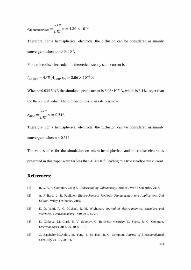
274
𝜎ℎ𝑒𝑚𝑖𝑠𝑝ℎ𝑒𝑟𝑖𝑐𝑎𝑙 =𝑟2𝐹
𝐷𝑅𝑇𝜈 = 4.30 × 10⁻²
Therefore, for a hemispherical electrode, the diffusion can be considered as mainly
convergent when σ<4.30×10⁻².
For a microdisc electrode, the theoretical steady state current is:
𝐼𝑠.𝑠,𝑑𝑖𝑠𝑐 = 4𝐹𝐷[𝐴]𝑏𝑢𝑙𝑘𝑟𝑒𝑙 = 3.86 × 10⁻⁹ 𝐴
When ν=0.035 V s-1, the simulated peak current is 3.98×10⁻⁹ A, which is 3.1% larger than
the theoretical value. The dimensionless scan rate σ is now:
𝜎𝑑𝑖𝑠𝑐 =𝑟2𝐹
𝐷𝑅𝑇𝜈 = 0.316
Therefore, for a hemispherical electrode, the diffusion can be considered as mainly
convergent when σ < 0.316.
The values of σ for the simulation on micro-hemispherical and microdisc electrodes
presented in this paper were far less than 4.30×10⁻², leading to a true steady-state current.
References:
[1] R. G. A. B. Compton, Craig E, Understanding Voltammetry, third ed., World Scientific, 2018.
[2] A. J. Bard, L. R. Faulkner, Electrochemical Methods: Fundamentals and Applications, 2nd
Edition, Wiley Textbooks, 2000.
[3] D. O. Wipf, A. C. Michael, R. M. Wightman, Journal of electroanalytical chemistry and
interfacial electrochemistry 1989, 269, 15-25.
[4] K. Cinková, M. Clark, S. V. Sokolov, C. Batchelor-McAuley, Ľ. Švorc, R. G. Compton,
Electroanalysis 2017, 29, 1006-1013.
[5] C. Batchelor-McAuley, M. Yang, E. M. Hall, R. G. Compton, Journal of Electroanalytical
Chemistry 2015, 758, 1-6.
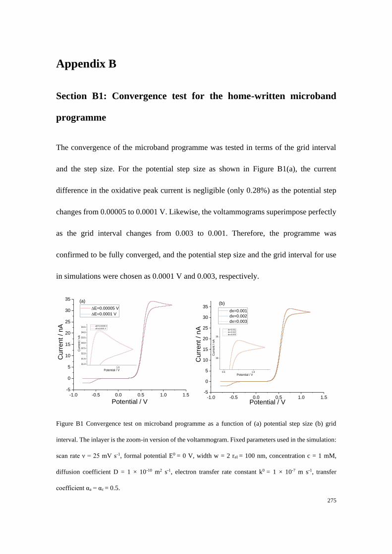
275
Appendix B
Section B1: Convergence test for the home-written microband
programme
The convergence of the microband programme was tested in terms of the grid interval
and the step size. For the potential step size as shown in Figure B1(a), the current
difference in the oxidative peak current is negligible (only 0.28%) as the potential step
changes from 0.00005 to 0.0001 V. Likewise, the voltammograms superimpose perfectly
as the grid interval changes from 0.003 to 0.001. Therefore, the programme was
confirmed to be fully converged, and the potential step size and the grid interval for use
in simulations were chosen as 0.0001 V and 0.003, respectively.
Figure B1 Convergence test on microband programme as a function of (a) potential step size (b) grid
interval. The inlayer is the zoom-in version of the voltammogram. Fixed parameters used in the simulation:
scan rate ν = 25 mV s-1, formal potential E0 = 0 V, width w = 2 rel = 100 nm, concentration c = 1 mM,
diffusion coefficient D = 1 × 10⁻¹⁰ m2 s-1, electron transfer rate constant k0 = 1 × 10⁻⁷ m s-1, transfer
coefficient αa = αc = 0.5.
-1.0 -0.5 0.0 0.5 1.0 1.5-5
0
5
10
15
20
25
30
35
1.0
31.0
31.5
32.0
32.5
33.0
33.5
34.0
34.5
Curr
ent / nA
Potential / V
E=0.00005 V
E=0.0001 V
Cu
rre
nt
/ n
A
Potential / V
E=0.00005 V
E=0.0001 V
(a)
-1.0 -0.5 0.0 0.5 1.0 1.5-5
0
5
10
15
20
25
30
35
0.5 1.0
30
35
Cu
rre
nt
/ n
A
Potential / V
dx=0.001
dx=0.002
dx=0.003
Curr
ent / nA
Potential / V
dx=0.001
dx=0.002
dx=0.003
(b)

276
Section B2: Blind tests
This section shows examples of the electrochemical measurement of width and length of
unknown band electrodes. The blind tests were run using ‘synthetic’ voltammograms
generated with known diffusion coefficients of reactant and product (D(A)=2D(B)= 1×10-
10 m2 s-1) as well as two different anodic transfer coefficients (αa=0.3, αa=0.4). The case
where αa=0.3 and αa=0.4 are shown in Section B2.1 and Section B2.2, respectively.
Section B2.1: Test 3 - Redox couple with low unequal diffusion coefficients (αa = 0.3,
αc = 0.7)
The voltammogram of the blind test is shown in Figure B2 for a band electrode width
unknown band width and length. The reactant and product have unequal diffusion
coefficients. The procedures of measuring the band width and length are shown below.
First, the known diffusion coefficients of reactant A and product B are 1×10⁻¹⁰ m2 s-1 and
0.5×10⁻¹⁰ m2 s-1, respectively. The anodic transfer coefficient is 0.3. Experimentally, these
parameters would be measured from steady-state micodisc voltammetry and Tafel
analysis.
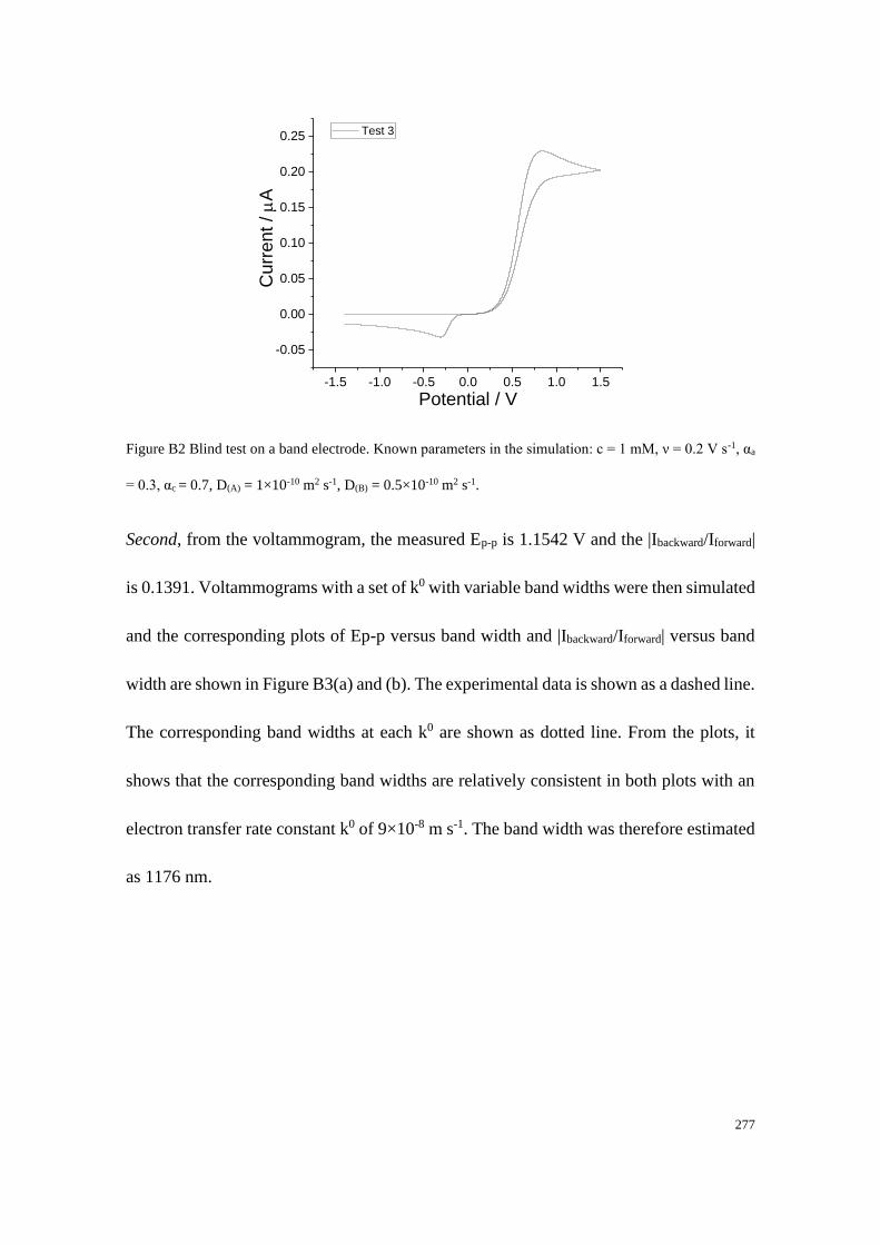
277
Figure B2 Blind test on a band electrode. Known parameters in the simulation: c = 1 mM, ν = 0.2 V s-1, αa
= 0.3, αc = 0.7, D(A) = 1×10⁻¹⁰ m2 s-1, D(B) = 0.5×10⁻¹⁰ m2 s-1.
Second, from the voltammogram, the measured Ep-p is 1.1542 V and the |Ibackward/Iforward|
is 0.1391. Voltammograms with a set of k0 with variable band widths were then simulated
and the corresponding plots of Ep-p versus band width and |Ibackward/Iforward| versus band
width are shown in Figure B3(a) and (b). The experimental data is shown as a dashed line.
The corresponding band widths at each k0 are shown as dotted line. From the plots, it
shows that the corresponding band widths are relatively consistent in both plots with an
electron transfer rate constant k0 of 9×10⁻⁸ m s-1. The band width was therefore estimated
as 1176 nm.
-1.5 -1.0 -0.5 0.0 0.5 1.0 1.5
-0.05
0.00
0.05
0.10
0.15
0.20
0.25
Cu
rre
nt
/
A
Potential / V
Test 3
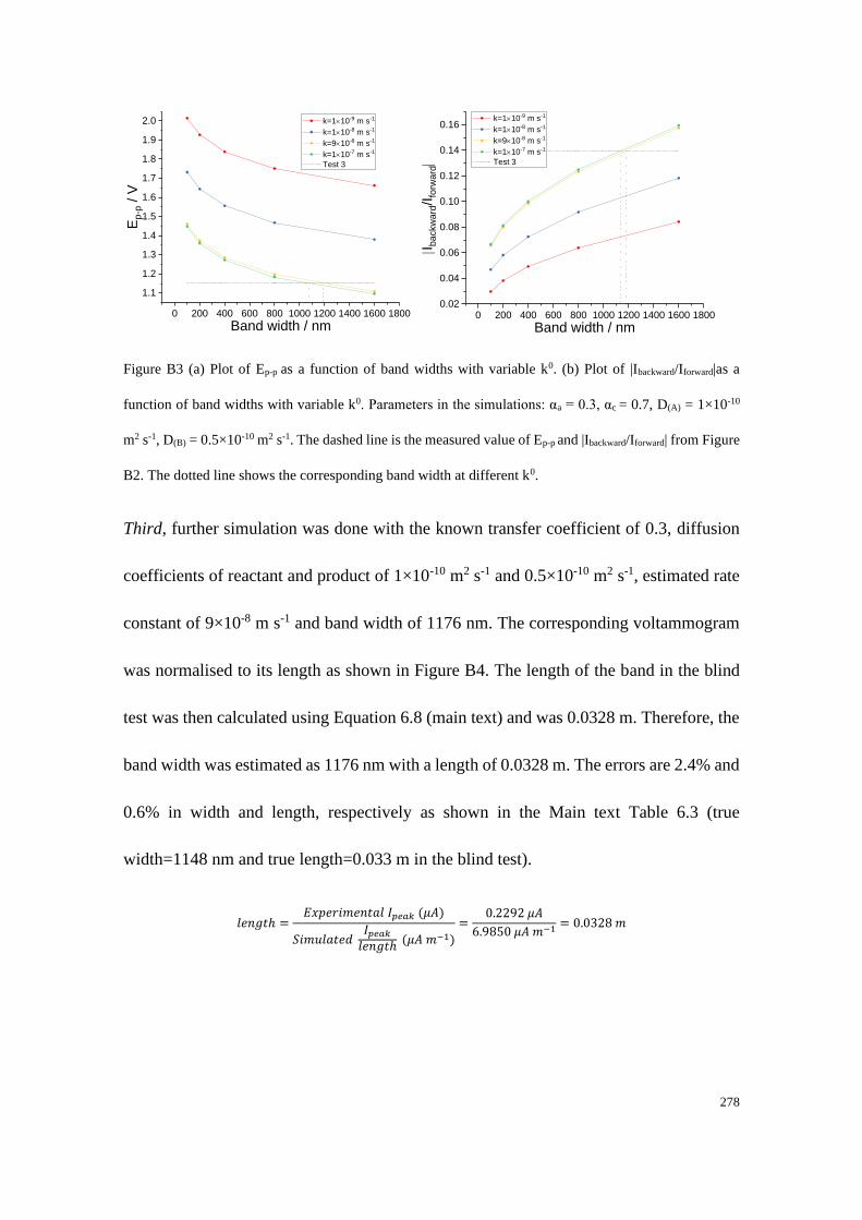
278
Figure B3 (a) Plot of Ep-p as a function of band widths with variable k0. (b) Plot of |Ibackward/Iforward|as a
function of band widths with variable k0. Parameters in the simulations: αa = 0.3, αc = 0.7, D(A) = 1×10⁻¹⁰
m2 s-1, D(B) = 0.5×10⁻¹⁰ m2 s-1. The dashed line is the measured value of Ep-p and |Ibackward/Iforward| from Figure
B2. The dotted line shows the corresponding band width at different k0.
Third, further simulation was done with the known transfer coefficient of 0.3, diffusion
coefficients of reactant and product of 1×10⁻¹⁰ m2 s-1 and 0.5×10⁻¹⁰ m2 s-1, estimated rate
constant of 9×10⁻⁸ m s-1 and band width of 1176 nm. The corresponding voltammogram
was normalised to its length as shown in Figure B4. The length of the band in the blind
test was then calculated using Equation 6.8 (main text) and was 0.0328 m. Therefore, the
band width was estimated as 1176 nm with a length of 0.0328 m. The errors are 2.4% and
0.6% in width and length, respectively as shown in the Main text Table 6.3 (true
width=1148 nm and true length=0.033 m in the blind test).
𝑙𝑒𝑛𝑔𝑡ℎ =𝐸𝑥𝑝𝑒𝑟𝑖𝑚𝑒𝑛𝑡𝑎𝑙 𝐼𝑝𝑒𝑎𝑘 (𝜇𝐴)
𝑆𝑖𝑚𝑢𝑙𝑎𝑡𝑒𝑑 𝐼𝑝𝑒𝑎𝑘
𝑙𝑒𝑛𝑔𝑡ℎ (𝜇𝐴 𝑚−1)
=0.2292 𝜇𝐴
6.9850 𝜇𝐴 𝑚−1 = 0.0328 𝑚
0 200 400 600 800 1000 1200 1400 1600 1800
1.1
1.2
1.3
1.4
1.5
1.6
1.7
1.8
1.9
2.0E
p-p
/ V
Band width / nm
k=110-9 m s-1
k=110-8 m s-1
k=910-8 m s-1
k=110-7 m s-1
Test 3
0 200 400 600 800 1000 1200 1400 1600 18000.02
0.04
0.06
0.08
0.10
0.12
0.14
0.16
Ib
ackw
ard
/Ifo
rwa
rd
Band width / nm
k=110-9 m s-1
k=110-8 m s-1
k=910-8 m s-1
k=110-7 m s-1
Test 3
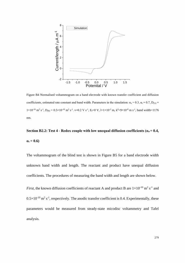
279
Figure B4 Normalised voltammogram on a band electrode with known transfer coefficient and diffusion
coefficients, estimated rate constant and band width. Parameters in the simulation: αa = 0.3, αc = 0.7, D(A) =
1×10⁻¹⁰ m2 s-1, D(B) = 0.5×10⁻¹⁰ m2 s-1. ν=0.2 V s-1, Ef=0 V, l=1×10⁻² m, k0=9×10⁻⁸ m s-1, band width=1176
nm.
Section B2.2: Test 4 - Redox couple with low unequal diffusion coefficients (αa = 0.4,
αc = 0.6)
The voltammogram of the blind test is shown in Figure B5 for a band electrode width
unknown band width and length. The reactant and product have unequal diffusion
coefficients. The procedures of measuring the band width and length are shown below.
First, the known diffusion coefficients of reactant A and product B are 1×10⁻¹⁰ m2 s-1 and
0.5×10⁻¹⁰ m2 s-1, respectively. The anodic transfer coefficient is 0.4. Experimentally, these
parameters would be measured from steady-state micodisc voltammetry and Tafel
analysis.
-1.5 -1.0 -0.5 0.0 0.5 1.0 1.5-2
0
2
4
6
8
Curr
ent/le
ngth
/
A m
-1
Potenital / V
Simulation
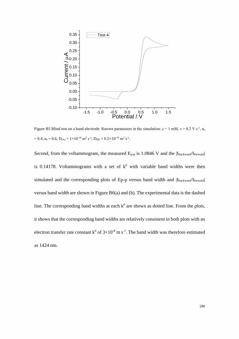
280
Figure B5 Blind test on a band electrode. Known parameters in the simulation: c = 1 mM, ν = 0.2 V s-1, αa
= 0.4, αc = 0.6, D(A) = 1×10⁻¹⁰ m2 s-1, D(B) = 0.5×10⁻¹⁰ m2 s-1.
Second, from the voltammogram, the measured Ep-p is 1.0846 V and the |Ibackward/Iforward|
is 0.14178. Voltammograms with a set of k0 with variable band widths were then
simulated and the corresponding plots of Ep-p versus band width and |Ibackward/Iforward|
versus band width are shown in Figure B6(a) and (b). The experimental data is the dashed
line. The corresponding band widths at each k0 are shown as dotted line. From the plots,
it shows that the corresponding band widths are relatively consistent in both plots with an
electron transfer rate constant k0 of 3×10⁻⁸ m s-1. The band width was therefore estimated
as 1424 nm.
-1.5 -1.0 -0.5 0.0 0.5 1.0 1.5-0.10
-0.05
0.00
0.05
0.10
0.15
0.20
0.25
0.30
0.35
Cu
rre
nt
/
A
Potential / V
Test 4
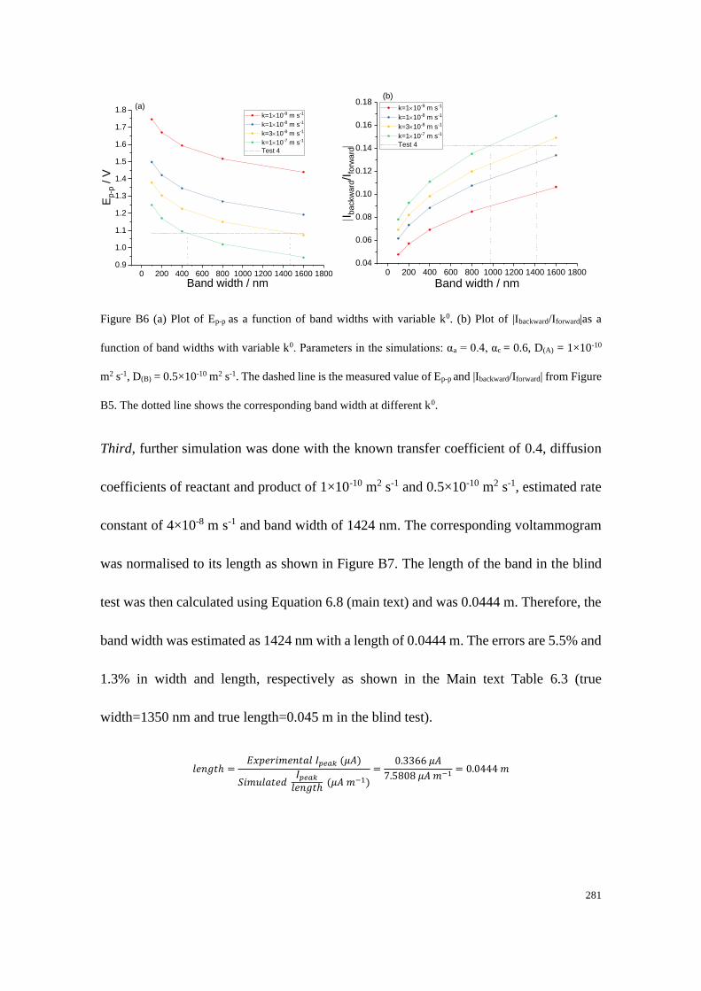
281
Figure B6 (a) Plot of Ep-p as a function of band widths with variable k0. (b) Plot of |Ibackward/Iforward|as a
function of band widths with variable k0. Parameters in the simulations: αa = 0.4, αc = 0.6, D(A) = 1×10⁻¹⁰
m2 s-1, D(B) = 0.5×10⁻¹⁰ m2 s-1. The dashed line is the measured value of Ep-p and |Ibackward/Iforward| from Figure
B5. The dotted line shows the corresponding band width at different k0.
Third, further simulation was done with the known transfer coefficient of 0.4, diffusion
coefficients of reactant and product of 1×10⁻¹⁰ m2 s-1 and 0.5×10⁻¹⁰ m2 s-1, estimated rate
constant of 4×10⁻⁸ m s-1 and band width of 1424 nm. The corresponding voltammogram
was normalised to its length as shown in Figure B7. The length of the band in the blind
test was then calculated using Equation 6.8 (main text) and was 0.0444 m. Therefore, the
band width was estimated as 1424 nm with a length of 0.0444 m. The errors are 5.5% and
1.3% in width and length, respectively as shown in the Main text Table 6.3 (true
width=1350 nm and true length=0.045 m in the blind test).
𝑙𝑒𝑛𝑔𝑡ℎ =𝐸𝑥𝑝𝑒𝑟𝑖𝑚𝑒𝑛𝑡𝑎𝑙 𝐼𝑝𝑒𝑎𝑘 (𝜇𝐴)
𝑆𝑖𝑚𝑢𝑙𝑎𝑡𝑒𝑑 𝐼𝑝𝑒𝑎𝑘
𝑙𝑒𝑛𝑔𝑡ℎ (𝜇𝐴 𝑚−1)
=0.3366 𝜇𝐴
7.5808 𝜇𝐴 𝑚−1 = 0.0444 𝑚
0 200 400 600 800 1000 1200 1400 1600 18000.9
1.0
1.1
1.2
1.3
1.4
1.5
1.6
1.7
1.8E
p-p
/ V
Band width / nm
k=110-9 m s-1
k=110-8 m s-1
k=310-8 m s-1
k=110-7 m s-1
Test 4
(a)
0 200 400 600 800 1000 1200 1400 1600 18000.04
0.06
0.08
0.10
0.12
0.14
0.16
0.18
Iba
ckw
ard
/Ifo
rward
Band width / nm
k=110-9 m s-1
k=110-8 m s-1
k=310-8 m s-1
k=110-7 m s-1
Test 4
(b)
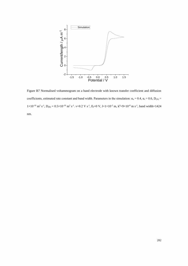
282
Figure B7 Normalised voltammogram on a band electrode with known transfer coefficient and diffusion
coefficients, estimated rate constant and band width. Parameters in the simulation: αa = 0.4, αc = 0.6, D(A) =
1×10⁻¹⁰ m2 s-1, D(B) = 0.5×10⁻¹⁰ m2 s-1. ν=0.2 V s-1, Ef=0 V, l=1×10⁻² m, k0=9×10⁻⁸ m s-1, band width=1424
nm.
-1.5 -1.0 -0.5 0.0 0.5 1.0 1.5-2
0
2
4
6
8
Cu
rre
nt/
len
gth
/
A m
-1
Potential / V
Simulation


![Zur elektrochemischen Aktivierungspolarisationzfn.mpdl.mpg.de/data/1/ZfN-1946-1-0433.pdf · The kinetics of electrode reactions Proc. Roy. Soc. [London] 169, 206 [1938], und Irreversible](https://static.cupdf.com/doc/110x72/605c3b1c189ec41fc0395dd1/zur-elektrochemischen-aktivie-the-kinetics-of-electrode-reactions-proc-roy-soc.jpg)