Università degli studi di Napoli “Federico II”
Università degli studi di Napoli ‘Parthenope’
Stratospheric dust collection by DUSTER (Dust in The Upper Stratosphere Tracking Experiment and Retrieval), a balloon-borne instrument, and laboratory analyses of collected dust.
Submitted for the degree of
Philosophiae Doctor in Aerospace Engineering
Alessandra Ciucci
Advisor: Prof. Pasquale Palumbo
Co-advisor: Prof. Frans J. M. Rietmeijer
Coordinator : Prof. Antonio Moccia

“Everything is determined, the beginning as well as the end, by forces over which we have no control. It is determined for insects as well as for the stars. Human beings, vegetables or cosmic dust, we all dance to a mysterious tune, intoned in the distance by an invisible piper”
Albert Einstein

Abstract ................................................................................................................................ 5
1 Stratospheric particles .................................................................................................... 7
1.1 Aerosols in stratosphere ......................................................................................................... 8
1.1.1 Terrestrial natural and anthropogenic particles .................................................................................... 10
1.1.2 Extraterrestrial particles ........................................................................................................................ 12
1.2 Studies of stratospheric aerosols .......................................................................................... 13
1.2.1 Remote sensing ..................................................................................................................................... 15
1.2.2 In-Situ collection .................................................................................................................................... 17
Conclusions ...................................................................................................................................... 19
2 DUSTER (Dust in the Upper Stratosphere Tracking Experiment and Retrieval) ................ 20
2.1 Aims ...................................................................................................................................... 21
2.2 Scientific and technical requirements ................................................................................... 21
2.3 DUSTER2008: the instrument ................................................................................................ 22
2.4 Sample holders (Blank and Collector) ................................................................................... 25
2.4.1 Structure ................................................................................................................................................ 26
2.4.2 Assembling............................................................................................................................................. 27
Conclusions ...................................................................................................................................... 29
3 Analytical techniques used for collected particles identification, manipulation and
characterization .................................................................................................................. 30
3.1 FE-SEM (Field Emission Scanning Electron Microscope) ........................................................ 31
3.2 EDX (Energy Dispersive X-rays) ............................................................................................. 35
3.3 SEM-FIB (Scanning Electron Microscope-Focused Ion Beam) ................................................ 36
3.4 Fourier Transform Infra-Red (FT-IR) spectroscopy ................................................................ 37
4 Sample holders pre- and post-flight characterization, laboratory procedures, including
sources of contaminations. .................................................................................................. 39
4.1 Characterization .................................................................................................................... 40
4.1.1 Problems during characterization of sample holders ............................................................................ 42
4.2 Curation ................................................................................................................................ 44
4.2.1 Description of the procedures to handle the sample holders ............................................................... 45
4.2.2 TEM grids disassembly ........................................................................................................................... 46
4.3 Sources of contamination ..................................................................................................... 47
4.3.1 Sources of contamination from the sample holder ............................................................................... 48
4.3.2 Source of contamination by FIB ............................................................................................................. 53
4.3.3 Sources of contamination from the flight train ..................................................................................... 54
Conclusions ...................................................................................................................................... 55
5 Sample collected during the June 2008 campaign: analyses results ................................ 56

5.1 Particle statistics and size distribution .................................................................................. 57
5.2 Morphology .......................................................................................................................... 60
5.3 Catalogue of raw data ........................................................................................................... 61
5.4 Data reduction ...................................................................................................................... 94
5.5 Discussions ...........................................................................................................................102
5.5.1 Terrestrial sources ............................................................................................................................... 109
5.5.2 Extraterrestrial sources ....................................................................................................................... 112
Conclusions .....................................................................................................................................114
6 DUSTER2009 instrument improvements and July 2009 campaign ................................ 116
6.1 The instrument ....................................................................................................................117
6.1.1 Sample holders .................................................................................................................................... 118
6.2 Characterization ...................................................................................................................121
6.3 Preliminary results (contamination and collected particles identification) ..........................123
Conclusions .....................................................................................................................................124
Conclusions and future developments ................................................................................ 125
Bibliography ...................................................................................................................... 127
Acknowledgements ........................................................................................................... 132

Abstract
The subject of this work is focused on the study of stratospheric dust with DUSTER (Dust in the
Upper Stratosphere Tracking Experiment and Retrieval) a balloon-borne instrument.
The stratospheric environment is an atmospheric layer placed in the range altitude 20-50 km. The
stratosphere is composed of aerosols (mostly H2SO4 and NOx) and refractory dust of different
nature: natural terrestrial dust, anthropogenic dust, and natural extraterrestrial dust (see Chapter
1 for more details).
The DUSTER project is aimed at uncontaminated collection of stratospheric dust particles, in the
submicron/micron range. The submicron/micron size range was chosen because: 1) it is poorly
studied so far; 2) particles of natural terrestrial origin in this size range are responsible of local and
global climate changing; 3) particles of natural extraterrestrial origin in submicron/micron range
suffer less the heating due to the entry in the Earth atmosphere and subsequently they are less
altered in the original physico-chemical characteristics.
The DUSTER scientific aim is to derive the size distribution, the concentration and the composition
of stratospheric dust, to study the natural and the extraterrestrial component. To reach its aim
DUSTER implies in-situ collection and sample recovering to perform laboratory analyses without
sample manipulation.
The technical requirement of the instrument are: capability to work autonomously during the
balloon flight in the range altitude of 30 – 40 km; capability to work at temperatures in the range -
40°C < T < 80°C and pressure in the range 3 – 10 mbar; sampling at least 20 m3 of air for at least
24 h of continuous working; samples storage and retrieval under contamination controlled
conditions (see Chapter 2 for more details).
The particles are captured based on the principle of inertial impact collection (without the use of
sticking materials) by a continuous flow created through the chamber.
DUSTER had a qualification flight in January 2006 from Kiruna (Sweden) and two scientific flights
from Svalbard (Norway) in June 2008 and July 2009.

This work is a report of the two scientific flights from the sample holder preparation to the
analyses of collected samples. In particular, it will deal with:
the sample holders structure, how to assemble them (see Chapter 2 for more details) and
their implementation for DUSTER 2009 campaign (see Chapter 6 for more details);
the instrument characteristics for DUSTER 2008 campaign and the improvements for
DUSTER 2009 campaign;
the curation, to ensure the contamination control, and the characterization of the sample
holders, to identify the particles actually collected from the spurious contamination (see
Chapter 4 for more details);
the techniques used to characterize the sample holder before and after the flights and to
analyze the sample collected (see Chapter 3 for more details);
the procedure to recognize the collected particles from the spurious contamination;
the sources of contamination due to the environment and to the sample holders
materials (see Chapter 4 for more details);
the data reduction of the analyses performed on samples collected during DUSTER 2008
campaign (see Chapter 5 for more details);
a very preliminary analysis to identify particles collected during DUSTER 2009 campaign
(see Chapter 6 for more details).
The strength of DUSTER is to collect particles in a boundary layer in which could be found particles
coming from extraterrestrial (e.g. interplanetary dust particles) and terrestrial environment (e.g.
volcanic ash) mixed in an environment clean by human pollution.

1 Stratospheric particles
The terrestrial atmosphere is divided into different layers diverse each other for altitude, pressure
and temperature. From the ground to the space environment there are: troposphere,
stratosphere, mesosphere, thermosphere and exosphere.
The troposphere and stratosphere extend from the ground until 50 km. In the troposphere the
temperature decreases with the altitude until -60 °C, in the stratosphere the temperature
increases until 0 °C (Figure 1.1) due to the presence of an ozone layer that absorbs the ultraviolet
radiation coming from the Sun.
In the mesosphere layer the temperature decreases until -90 °C; in this layer the destruction of
meteors that enter Earth’s atmosphere occurs and the light elements relative abundances slowly
increase to the detriment of the heaviest. In the thermosphere the temperature increases; this is
considered the last atmospheric layer. Above 100 km, the environment is very rarefied and it is
possible to put a spacecraft in orbit around Earth. The exosphere is a range in which there is a
gradual passage from atmosphere to the space environment.
This work is focuses on stratosphere. It contains aerosols typically in the size range 0.1 – 1 µm,
and a solid component (hereinafter, particles) that can be larger than 1 µm. The stratospheric
particles can be of different origins: natural terrestrial, anthropogenic and extraterrestrial.
Stratosphere is relatively accessible and close to the surface and at the same time it is a clean
environment where to collect particles for laboratory studies with a significant fraction of
extraterrestrial materials. Finally, stratospheric particles are relatively poorly studied, having in
any case strong impact on atmosphere physical status and chemical processes.
In this chapter the different kind of particles populating the stratosphere are presented together
with the experiments performed up to now in situ or through sample return to study the
stratospheric environment.
Figure 1.1 Molecular-scale temperature as a function of geopotential altitude (US Standard Atmosphere
1976)

1.1 Aerosols in stratosphere
The US Standard Atmosphere model defines the typical value for temperature, pressure, density
and composition of the different layers of Earth’s atmosphere. In Table 1.1 the typical
concentration of troposphere constituents near the Earth’s surface are reported, but that values
change with altitude and latitude.
The Nitrous Oxide is between 250 – 100 ppbv in the altitude range of 13 -18 km. The Nitric Oxide
and the Nitrogen Dioxide have a similar behavior: the NO has an estimated mixing ratio varying
from about 0.1 ppbv at 16 km and 5 ppv at 40 km; the NO2 goes from 1 – 10 ppbv in the altitude
range 12 - 28 km and increase from 20 -28 km. The Nitric Acid vapor is 2 ppbv at about 18 km and
5 ppbv at 24 km maintaining an high concentration until 30 km. Instead Hydrogen reaches the
highest value at 28 km and decreases above it. Carbon Monoxide has both anthropogenic and
natural sources, it has been found in troposphere, while CO2 can be found in stratosphere too, but
0.6 ppmv less than in troposphere (US Standard Atmosphere 1976).
In Figure 1.2 the Ozone model density is shown; it reaches the maximum concentration in lower
stratosphere, the high presence of Ozone in unpolluted regions near the Earth’s surface is
probably formed in stratosphere and brought down by the vertical transport process; the
presence of water vapor in stratosphere is attribute to this process.
A study of aerosol type, concentration and size distribution that combined theoretical data with
observations was done using two balloon-born instruments: Spectroscopie d’Absorpion Lunaire
pour l’Observation des Minoritaires Ozone et NOx (SALOMON), and Laboratiorie de Météorologie
Dynamique (LMD).
Figure 1.2 Mid-latitude ozone model density as a function of height

Constituent Typical concentration in parts per billion per
volume (ppbv)
N2O 270
NO 0.5
NO2 1
H2S 0.05
NH3 4
H2 500
CH4 1500
SO2 1
CO 190
CO2 3.22 x 10⁵
O3 40
Table1.1 Concentration of tropospheric constituent near the Earth’s surface (US Standard Atmosphere
data)
These experiments confirmed the presence of aerosols around 30 km. The unexpected results
were: particles with a size dimensions bigger than 1 µm (Figure 1.3); particles composed of a
mixture of H2SO4 and water vapor, typical of aerosol present in lower stratosphere and not
suppose to be at that altitude (Renard et al. 2005). They hypothesized that the identified particles
can be soot of terrestrial or extraterrestrial origin, from coagulation process or from vaporization
of micrometeorites during entry in atmosphere respectively. The data provided by SALOMON and
LMD suggested that the main population of solid particles present in middle stratosphere can be
originated by interplanetary medium.
At any given time in stratosphere there are different kinds of solid particles: some are originated
at the Earth’s surface due to natural and anthropogenic processes, others are of extraterrestrial
origins, viz. (1) a wide range of different interplanetary dust particles, (2) condensed meteoric
dust from sublimating meteors that so far has eluded collection, (3) residues of meteorite and
micrometeorite ablation in the mesosphere or cometary fragments.
The alteration of Stratospheric Aerosol (SA) population may cause alteration in the global
stratospheric dynamics (Pitari et al. 1993), the ozone depletion (Hofmann et al. 1993, Chandra
1993), the stratospheric heating (Angell 1997, Parker e Brownscombe 1983) and solar radiance

variations (as during Pinatubo eruption of June 1991 (Dutton and Christy 1992)). For these
reasons it is important to study and characterize stratospheric particles and their dynamics.
Figure 1.3 Vertical distribution of six diameter class of aerosols obtained on 22 October 2001 by the LMD
counter (after Renard et al. 2005)
1.1.1 Terrestrial natural and anthropogenic particles
The particles of natural terrestrial origins are typically volcanic ashes, wind-blown dust and
condensed aerosols. The Stratospheric Sulfate Aerosols (SSA) are produced by the interaction
between SO2 and water condensed particles; sulfur dioxide can be transported from the tropical
tropopause, or photochemically produced in the mid-stratosphere after ultraviolet photolysis of
carbonyl sulfide (Rodhe et al. 1985).
The presence of volcanic ashes in the stratosphere and their effects were studied after Fuego
(14°N, October 1974, 3–6 Tg of aerosol) eruption and especially during the El Chichòn (17°N, April
1982, 12 Tg of aerosols) and Pinatubo eruptions (15 °N, June 1991, 30 Tg of aerosols) (McCormick
et al., 1995). Following Kerr (1983), the volcanic cloud after El Chichòn eruption extended in the
latitude range of 10°S and 30°N; a temperature rise of 3°C was measured around 26 km and its
cause was almost entirely attributed to sunlight absorption. After Pinatubo eruption the
enhancement of stratospheric aerosol caused a disturbance of the twilight sky radiative field
(Mateshvili et al. 2005) and the increasing of the temperature (Saxena et al. 1997).
A size distribution of SA after Pinatubo eruption and its changing with years was provided by
Deshler (2008). One year lather the eruption, the SA were well mixed, particles > 0.78 µm were
observed over 20 km; 15 years lather particles > 0.5 µm were observed in stratosphere and there

is a difference in concentration of Condensation Nuclei (CN) in particles > 0.15 µm and increasing
with size (Figure 1.4).
The changing of size distribution during time and the removal of same particles from stratosphere
is due to the gravitational settling; the nucleation and condensation of aerosols increase the size
and the heaviest particles are moved close to the tropopause and subsequently moved in the
troposphere by the exchange process between troposphere and stratosphere.
Figure 1.4 Differential number (cm− 3), surface area (µm2 cm− 3), and volume (µm3 cm− 3) distributions, as a
function of dlog10(r) derived from fitting bimodal lognormal size distributions to in situ optical particle
counter measurements at 21 km above Laramie, Wyoming (Deshler et al., 2003). The cumulative number
distribution (the blue data points), and the fitted distribution (the blue dashed line). The size distributions
are representative of measurements a) one year, b) 3 years, and c) 15 years after the Pinatubo eruption.
During volcanically quiescent periods SA (in particular sulfuric acid and water vapor) affect the
budget of several trace of gases, in particular NOx, while after volcanic activity SA may increase
the abundance of chlorine (Hanson and Lovejoy, 1995).
Particles of anthropogenic origins are typically residual of solid-fuel rocket exhaust, coal- and oil-
burning and power plants residuals. Evidences of propellant residuals particles came from the first
experiment of collection in stratosphere (at 34 km) performed by Brownlee in 1970. The majority
of the particles collected by that experiment in the size range 3 – 8 µm were spheres of Al2O3
originated by fuel residuals (Brownlee et al. 1973).
The others typical sources of particles of anthropogenic origin are power plant combustion and
coal combustion products (CCP). In Svalbard Islands there are coal power plants that produce coal
fly ash and heavy metal pollution in the region, as found studying sediments of the iced Lake of
Bolterskardet (Qing et al. 2006). In China, where coal is the basic energy source (about 84% of
total production), the presence of Fluorine pollution was studied because of its harmful effects;
when the coal is burnt at mid-low temperature (800 - 1200 °C) power station, only 20% of

Fluorine remain in the cinder and the rest is divided between 5% trapped in coal fly ash and 75%
directly injected in the atmosphere (Luo et al. 2002).
All these components could be found on stratosphere because of the convective upward
transport from tropical tropopause (Pitari et al. 1993).
1.1.2 Extraterrestrial particles
The sources of dust population are comets and asteroids (from the inner Solar System), Kuiper
belt dust and interstellar dust (from outer Solar System).
Meteorites or Interplanetary Dust Particles (IDPs) are fragment of rocks and metals from other
bodies in the Solar System that have fallen to the Earth and survive to the passage through the
atmosphere. The difference is mainly the size, the IDPs being typically 10 – 100 µm while
meteorites can reach several meters. The IDPs can be originated by collision between small
bodies, such as bodies in the main asteroid belt, meteoroids impact on the asteroids and
interaction with near Earth asteroids, or by sublimation of active comet nuclei during the
perihelion transit (Rietmeijer 2000).
These particles are the responsible of the Zodiacal light. It is the diffuse light in the night sky,
enhanced in the ecliptic, also called Zodiacal line (from which the name of the effect). The light is
actually extended across the entire night sky, but being the particles distributed principally in the
Sun equatorial plane the light is stronger in the ecliptic line. Due to the Pointing-Robertson effect,
these particles has a spiral motion toward to the Sun; for this reason the density of particles
between 0.1 – 100 µm increases with decreasing distance from the Sun proportional to r-1 (where
r is the distance from the Sun).
The particles in this size range are the most abundant in 1 AU range from the Sun (Rietmeijer
2002). The heating and melting of the particle during the deceleration is function of the size,
density, mineralogy, entry angle and entry velocity (Love and Brownlee 1994). Being the IDPs very
small (<100 µm), they are able to survive to the atmospheric entry with some thermal alteration;
instead the meteoroids (in a size range from 100 µm up to same meters) will not survive to the
atmospheric entry and typically produced ablation debris.
The interstellar dust is originated by the loosing mass of stars that are in the last evolutionary
stage or by supernovae explosion. The gas flux from the stars, during the expansion, cools down
and reaches the condition to allow solid dust particles condensation. Interstellar dust was
identified at 5 AU by the Ulysses dust detector (Grün et al., 1993), and inside 1AU it is estimated
less abundant than in the outer Solar System (Grün et al., 1994). In particular at 1AU the
interstellar dust component is less than 3% of the interplanetary component (McDonnel & Berg,
1975).
The IDPs collected in stratosphere are classified combining the chemical composition and the
morphological class (Figure 1.5). They can be chondritic or non chondritic IDPs.
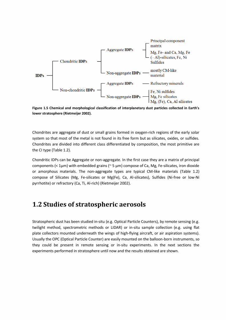
Figure 1.5 Chemical and morphological classification of interplanetary dust particles collected in Earth's
lower stratosphere (Rietmeijer 2002).
Chondrites are aggregate of dust or small grains formed in oxygen-rich regions of the early solar
system so that most of the metal is not found in its free form but as silicates, oxides, or sulfides.
Chondrites are divided into different class differentiated by composition, the most primitive are
the CI type (Table 1.2).
Chondritic IDPs can be Aggregate or non-aggregate. In the first case they are a matrix of principal
components (< 1µm) with embedded grains (~ 5 µm) compose of Ca, Mg, Fe-silicates, iron dioxide
or amorphous materials. The non-aggregate types are typical CM-like materials (Table 1.2)
compose of Silicates (Mg, Fe-silicates or Mg(Fe), Ca, Al-silicates), Sulfides (Ni-free or low-Ni
pyrrhotite) or refractory (Ca, Ti, Al-rich) (Rietmeijer 2002).
1.2 Studies of stratospheric aerosols
Stratospheric dust has been studied in-situ (e.g. Optical Particle Counters), by remote sensing (e.g.
twilight method, spectrometric methods or LIDAR) or in-situ sample collection (e.g. using flat
plate collectors mounted underneath the wings of high-flying aircraft, or air aspiration systems).
Usually the OPC (Optical Particle Counter) are easily mounted on the balloon-born instruments, so
they could be present in remote sensing or in-situ experiments. In the next sections the
experiments performed in stratosphere until now and the results obtained are shown.

Species CI type CM type
SiO2 22.69 28.97
TiO2 0.07 0.13
Al2O3 1.70 2.17
Cr2O3 0.32 0.43
Fe2O3 13.55 -
FeO 4.63 22.14
MnO 0.21 0.25
MgO 15.87 19.88
CaO 1.36 1.89
Na2O 0.76 0.43
K2O 0.06 0.06
P2O5 0.22 0.24
H2O+ 10.80 8.73
H2O- 6.10 1.67
Fe0 - 0.14
FeS 9.08 5.76
C 2.80 1.82
S (element) 0.10 -
NiO 1.33 1.71
CoO 0.08 0.08
SO3 5.63 1.59
CO2 1.50 0.78
TOTAL 98.86 99.82
Table 1.2 Average chemical compositions of chondrites CI and CM type.

1.2.1 Remote sensing
From late 1979 two similar experiments studied the atmosphere with remote sensing techniques:
the SAGE I (Stratospheric Areosol Gas Experiment 1979-1981) and SAM II (Stratospheric Aerosol
Measurements 1978-1993). They are satellite experiments based on Sun photometers to measure
the extinction of solar radiation produced by aerosol in the Earth atmosphere (McCormick et
al.1979). Because of the attenuation of tropospheric clouds, data are available above 5 km; the
variation of 1 µm tropospheric aerosol with latitude, season and altitude as well as changes due
to volcanic injection of material into the stratosphere has been highlighted (Kent et al. 1988).
From 1981 to 1985, during a period of strong volcanic activity (El Chichòn and Pinatubo
eruptions), the stratospheric dust was tracked using the twilight sounding method (TSM) capable
of covering an altitude range between 20 and 140 km (Mateshvili and Rietmeijer 2002). This
method allowed to study the distribution of volcanic dust and the life time of that particles into
the stratosphere. The volcanic ash had the maximum concentration in stratosphere immediately
after the eruption and decays in few months; instead the condensed aerosols have the maximum
few months after the volcanic event.
A campaign of LIDAR (Light Detection and Ranging) observations was performed from Thule in
Greenland through the period 1990-1997 to study the Polar Stratospheric Clouds (PSCs). They
observed that the PSC formation depends by the evolution of polar vortex, altitude, temperature
and on the variable structure (they noted that a kind of PSC formed mainly after Pinatubo
eruption). From the observation it was derived that the PSCs were made of crystals less than 2 µm
in size (more than 2 µm appears unlikely) with a water (more than expected) and nitric acid
composition (Di Sarra et al. 2002).
The two balloon borne instruments AMON (Absorbition by the Minor components Ozone and Nox
1991-2003) and SALOMON (Spectroscopie d’Absorbition Lunaire pour l’Observation des
Minoritaries), are designed to perform measurements of stratospheric trace-gas species (O3, NO2,
NO) in the polar vortex in UV-VIS range. They concluded that each flight had its own peculiarity
depending on events, such as volcanic injections, and that most spectral signatures differ
significantly from the background aerosol (Berthet 2002).
During the same period (April - May 1998 and September 1999) there were same experiments on
stratospheric aerosol managed with a laser ion mass spectrometer on board of an aircraft from 5
to 19 km. The instrument collected more than 2500 spectrum of aerosol between 0.2 - 3 µm.
Those spectra suggest that many particles may contain extraterrestrial material coming from
meteoritic ablation, confirming the descending of material from mesosphere to stratosphere, and
the presence of mercury at 19 km altitude, showing that the terrestrial emission come up into the
lower stratosphere (Murphy et al. 1998). Taking into consideration the composition of typical
chondrites and the ablation phenomena, it results that in lower stratosphere until the sulphates
layer the material is mostly of terrestrial origin, and in upper stratosphere the sulphate is
dominated by the extraterrestrial component (Figure1.6) coming from ablation of
micrometeorites (Cziczo et al. 2001).

Figure 1.6 Typical positive ion mass spectra. (A) Stratospheric aerosol particle that contained meteoritic
material. (B) Ground meteorite particle composed of H-group chondritic matter (Field Museum of Natural
History sample Me 2076) dissolved in 65 wt % sulfuric acid such that there was ≤ 1.0 wt% Fe in solution
(some fraction, possibly SiO2, remained visibly undissolved). (C) Artificial meteorite particle prepared in
the laboratory that was 65 wt % sulfuric acid, 0.75 wt % Fe, 0.23 wt % Mg, and minor species in the
abundance found in chondritic meteorites with respect to the given iron concentration. Particle mass is
balanced by H2O in all cases. (Courtesy of Cziczo et al 2001).
In-situ observations of lower stratosphere were done within the Arctic and Antarctic polar
vortexes. In 1987 a balloon-borne instrument with condensation nucleus counter (CNC) and eight
channel aerosol detectors were flown from McMurdo station in Antarctic until 22 km altitude,
and in 1989 the same instrument was flown from Kiruna (Sweden 68°N) until 31 km altitude. The
results from Antarctic zone show two different aerosol types, large particles of nitric acid (~1 µm)
and small sulphate particles; under -79°C the two types are melted, and under -85°C the
concentration of the two distributions grow up suggesting the simultaneous nucleation and
growth phenomena (Hofmann et al. 1989 ). The results of Arctic zone are very similar to the
Antarctic zone, they found strong level of CN above 18 km suggesting homogeneous and ionic
nucleation (Hofmann et al. 1990). In the Arctic zone also flown on January and February 1989 an
air-borne instrument, compose of a passive cavity aerosol spectrometer and CNC. The results
showed that it seems to exist, in upper troposphere and lower stratosphere, a region of newly
formed small (0.02 – 1 µm) particles (Wilson et al. 1992), moreover the CN particles production is
important for Polar Stratospheric Clouds (PSC) formation and the concentration can affect PSC
properties (Wilson et al. 1990). More recently, from January to March 2003, an aircraft-borne
instrument was flown from Kiruna (Sweden) for in-situ measurements of Arctic lower
stratosphere (10 - 20.5 km altitude) inside and outside the polar vortex. The instrument was
composed of a two channel aerosol counter COPAS (COndensation PArticle counter System) with

a cut off of 0.01 µm and a modified Forward Scattering Spectrometer Probe FSSP-300 able to
measure aerosol particles between 0.4 - 23 µm. The COPAS experiment confirmed the aerosol
nucleation above 19 km, and detect a fraction of 58-76% of non-volatile particles inside the vortex
and 12-45% outside. This difference was attributed to the vertical transport of meteoritic material
from mesosphere to the lowest level of polar vortex (Curtius et al. 2005).
1.2.2 In-Situ collection
During the last 50 years there have been research projects aimed at study aerosol and
stratospheric dust in laboratory, so they need sample return experiment. For this reason several
balloon born instruments and special collector for rockets and airplanes were developed.
Junge at al. (1961) sampled the atmosphere until 30 km of altitude with a cascade inertial
impactor carried aloft on a stratospheric balloon, and used an optical particle counter (OPC) to
determine the concentration and the vertical profile of aerosol particle <0.1 µm. The experiment
collected particles in a constant size distribution, with a maximum in the range between 0.01-0.1
µm. The particles can be divided into three major classes: (1) particles <0.1µm from the
troposphere; (2) particles in the range (0.1-1.0) µm formed within the troposphere, the analyses
shown composition based on sulphur with traces of iron and silicon; (3) particle >1.0 µm of
extraterrestrial origin (this last had a low frequency and for this reason less studied in this
experiment).
Brownlee et al. (1973) collected stratospheric particles at about 35 km of altitude using a rocket,
mostly Al2O3 spherical particles and a 10% of IDPs; the spheres are anthropogenic particles
produced by burning fuel rockets and lying in the altitude range 25-35 km with a density of 10-2m-3
(Brownlee et al. 1976).
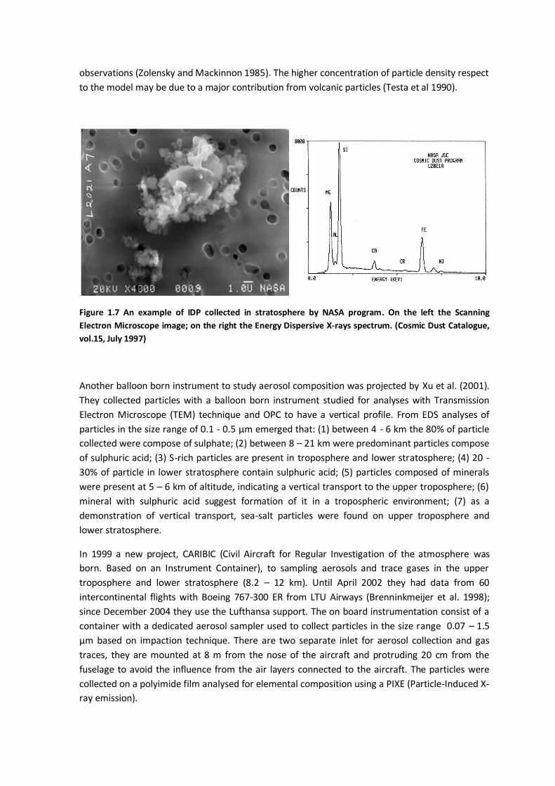
NASA has a long-term stratospheric dust collection program using high-flying (WB and U2) aircraft
fitted with inertial-impact, flat-plate collectors coated by high viscosity silicon oil layer to collect
dust particles at about 20 km altitude (Zolensky and Warren 1994). The collected solid dust
particles range between ~2 and 150 µm of natural extraterrestrial (comic dust) and terrestrial
origins and anthropogenic origins, e.g. aluminium or aluminium oxide spheres that are solid rocket
effluents (Mackinnon et al. 1982, Zolensky and Mackinnon 1985, Zolensky et al. 1989). The
collected particles receive a provisional identification based on their morphological, optical and
chemical properties (Figure1.7) and are then listed in the NASA Johnson Space Center catalogues
(Cosmic Dust Catalogues, volumes 1 through 17).
Testa et al. (1990) developed a balloon-borne instrument, with a collecting area made of a
nuclepore membrane filter (NMF) and nine TEM grids made of beryllium and carbon film. The
NMF was spattered with silver to make the surface more conductive and useful for Scanning
Electron Microscope (SEM) and Analytical Transmission Electron Microscope (ATEM) analyses.
The particles collected are in the size range 0.045-1.0 µm, mostly of particles from volcanic
injections (Rietmeijer, 1993). The measured particles density was much higher (10-105 times) than
the concentrations predicted by models of Hunten et al. (1980) but they were close to the in-situ
observations (Zolensky and Mackinnon 1985). The higher concentration of particle density respect
to the model may be due to a major contribution from volcanic particles (Testa et al 1990).
Figure 1.7 An example of IDP collected in stratosphere by NASA program. On the left the Scanning
Electron Microscope image; on the right the Energy Dispersive X-rays spectrum. (Cosmic Dust Catalogue,
vol.15, July 1997)
Another balloon born instrument to study aerosol composition was projected by Xu et al. (2001).
They collected particles with a balloon born instrument studied for analyses with Transmission
Electron Microscope (TEM) technique and OPC to have a vertical profile. From EDS analyses of
particles in the size range of 0.1 - 0.5 µm emerged that: (1) between 4 - 6 km the 80% of particle
collected were compose of sulphate; (2) between 8 – 21 km were predominant particles compose
of sulphuric acid; (3) S-rich particles are present in troposphere and lower stratosphere; (4) 20 -
30% of particle in lower stratosphere contain sulphuric acid; (5) particles composed of minerals
were present at 5 – 6 km of altitude, indicating a vertical transport to the upper troposphere; (6)
mineral with sulphuric acid suggest formation of it in a tropospheric environment; (7) as a
demonstration of vertical transport, sea-salt particles were found on upper troposphere and
lower stratosphere.
In 1999 a new project, CARIBIC (Civil Aircraft for Regular Investigation of the atmosphere was
born. Based on an Instrument Container), to sampling aerosols and trace gases in the upper
troposphere and lower stratosphere (8.2 – 12 km). Until April 2002 they had data from 60
intercontinental flights with Boeing 767-300 ER from LTU Airways (Brenninkmeijer et al. 1998);
since December 2004 they use the Lufthansa support. The on board instrumentation consist of a
container with a dedicated aerosol sampler used to collect particles in the size range 0.07 – 1.5
µm based on impaction technique. There are two separate inlet for aerosol collection and gas
traces, they are mounted at 8 m from the nose of the aircraft and protruding 20 cm from the
fuselage to avoid the influence from the air layers connected to the aircraft. The particles were
collected on a polyimide film analysed for elemental composition using a PIXE (Particle-Induced X-
ray emission).

They investigated potassium, iron and sulphur concentration in relation to potential vorticity (PV)
of the air mass and respect to the seasons. The results were that iron and potassium shown no
measurable change with the increasing of PV, but had a peak in concentration during March-June;
instead sulphur increase with the increasing of PV and shown a peak of concentration in the same
months but not as strong for the other elements. The sulphur at this altitude is produced by three
sources: the sulphur particulate by carbonyl sulphide (OCS) contribution, particulate made up of
sulphur dioxide transported across the tropical tropopause and extratropical tropopause
(Martinsson et al. 2005).
Conclusions
From all those experiment managed into troposphere and stratosphere we learn that: there is a
mutual exchange from mesosphere to upper stratosphere and from troposphere to lower
stratosphere; volcanoes ejecta arrive until upper stratosphere; stratosphere aerosol are mixed
with extraterrestrial materials coming from micrometeoroids ablation and evaporation.
The tracking and monitoring experiments in the Arctic and Antarctic polar vortex regions provided
a wealth of information on the upper stratospheric and mesospheric interactions, and about PSCs
formation and composition, but they did not collected particles for detailed laboratory
characterization. Dust particles could provide substrates for atmospheric chemistry of
condensable gases and they may play a role in the removal of sulphuric acid above ~40 km
altitude (Plane 2003). Meteoroid and other dust reach their maximum concentrations in the
mesosphere of the Arctic and Antarctic polar vortexes during the wintertime by moving dust from
one to the other region back and forth.
From the literature few collection experiments emerge and the NASA long term program does not
operate in the upper stratosphere. This left a gap in our understanding of the upper stratosphere
for what concern the solid particulates, their size, morphology, surface properties, chemistry, the
proportions of glass to mineral ratio, and their mineralogy. For this reasons the upper
stratosphere remains poorly sampled.
Any dust sampling instruments functioning in these environments needs to operate in an
autonomous operation mode, must have a efficient and reliable contamination control system
and the collected nanometer- to micrometer-scale dust must be stored safely during the period of
collector retrieval in the field and opening in the laboratory. In this frame the DUSTER (Dust in the
Upper Stratosphere Tracking Experiment and Retrieval) experiment was designed, with the aim to
collect dust in the boundary layer in which there is material coming up (from Earth’s surface) and
coming down from mesosphere.

2 DUSTER (Dust in the Upper Stratosphere
Tracking Experiment and Retrieval)
In this chapter I will discussed the DUSTER experiment from the first idea, in 2006, to perform a
long term project for stratospheric aerosols collection, to the successful flight performed in June
2008 Svalbard campaign.
Aims, scientific and technical requirements who brought to the DUSTER2oo8 instrument will be
discussed. The instrument from the mechanical and functional points of view will be described.
Particular attention will be given to the core of DUSTER2008, the collecting chamber, the sample
holders and their accommodation inside the chamber. For what concerns the sample holders, the
details will be discussed in the last section, together with the mounting and contamination control
procedure.
Finally, the conclusions will describe the goals of DUSTER2008 and the related scientific and
technical requirements and their relation with the previous experiment for stratospheric aerosol
study.
2.1 Aims
DUSTER is a balloon-borne experiment developed to collect the stratospheric aerosol in the
poorly studied region in the elevation range of 30 – 40 km. The principal aim is to detect and
study the different typology of particles (natural - volcanic, anthropogenic, extraterrestrial -
micrometeorites and IDPs) present in that stratospheric region.
DUSTER has to be light, little and totally autonomous; it has to collect particle in the size range 0.1
- 10 µm without contamination and manipulation; and, possibly, it has to be cheap.
Good results have been obtained for what concern the miniaturization; it goes from the prototype
DUSTER2006 (0.6x0.6x0.46) m3 in size and 65 kg in weight, to the operative versions DUSTER2008
that is almost ¼ in volume of the prototype, (0.41x0.41x0.31) m3 in size and 30 kg in weight. It is
able to fly autonomously, with a little balloon (10.000 m3), or as a piggyback of another
instrument and in both cases it can be autonomous. This is important to ensure a doable and
repeatable program to collect particles in different areas and season.
The first scientific flight (DUSTER2008) collected particles in the size range 0.5 – 150 µm, and they
are uncontaminated and well distinguishable from potential accidental contamination present on
collection substrate. Preliminary analyses can be done successfully without manipulation of the
samples. As we will see for specific analyses the samples need to be manipulated, but it can be
done under contamination control.
All DUSTER versions are totally designed and assembled in laboratory, with customized
commercial elements and tools developed for vacuum environment. This allows to create a very
cheap and autonomous instrument.
2.2 Scientific and technical requirements
To have a successful collection flight, the instrument has to meet some scientific and technical
requirement.
It needs to work in autonomous operation mode, must have a reliable contamination control
system and the collected nanometer to micrometer scale dust must be stored safely during the
period of instrument retrieval and opening in laboratory.
It has to be able to work in a wide range of temperature (-40°C <T< 50°C) at the altitude between
30 and 40 km. Last but not least, DUSTER has to be compatible with collection of aerosols in the
size range between 0.1 and 10 µm; to allow the collection of hundreds of those particles, an air
volume collection of about 20 m3 is required.
The collection is focused on the given size range for the following reasons:
it is a size range poorly study especially with laboratory instrumentation;

the IDPs on this size range have the peculiarity to suffer lower heating during
entry in atmosphere with respect to larger particles and in this manner they are
not processed. The probability of surviving unaltered during entry is significantly
higher for particle in the size range 0.1 – 1 µm (Flynn 1997), and this allows to
study the particles in their original status;
it is demonstrated by the in-situ data of Ulysses and Galileo missions that, for
interstellar grains, smaller particles are dominant in number and mass with
respect to the large particles (Landgraf et al., 2000) (Figure 2.1);
aerosol density measured in this conditions allow to collect 10-1 particles/cm3 in
the size range of 0.1 - 1 µm (Renard et al. 2005), and about 2x10⁻⁴ particles/cm3
for the solid component greater than 10 µm (Pueschel et al. 1995, Biermann et
al. 1996).
Figure 2.1 Ulysses and Galileo Data (Landgraf et al. 2000). The red line is the expected from DUSTER
collection.
2.3 DUSTER2008: the instrument
DUSTER prototype was developed looking at the previous experience of Testa et al. (1990).
DUSTER2006 (Figure 2.2) had a qualification flight on January 2006 from Kiruna (Sweden) thanks
to CNES (Centre National d’Etudes Spatiales) and Esrange Space Centre balloon campaign. It was
in operative mode for 2h at the floating altitude of 28-29 km. The aim of the flight was to test the
operation and the capability of retrieval. Inside the instrument, the sample holders were present
too, but there were no significant scientific data due to the very short collection time and
insufficient characterization of contamination before the flight.

Figure 2.2 DUSTER2006 recovery.
The new miniaturized instrument, DUSTER2008, was launched from Longyearbyen (Svalbard
Islands) on June 2008 in a dedicated ASI (Italian Space Agency) balloon campaign (Figure 2.3). It
flew for 3.5 days and remained in operative mode for 55h at a floating altitude of about 37 km
with a flow rate of 1 m3/h before being recovered in Thule (Greenland) (Figure 2.3). From this
flight we were able to collect particles for following scientific analyses.
Figure 2.3 Launch chain (the big image) and trajectory (the little image on left) of DUSTER2008
instrument.

The instrument structure is a box realized with aluminium bars Bosh Rexroth and an aluminium
plates that divided the box in two ambient; the box is covered with 5 aluminium panels, 4 of them
wrapped with thermal isolation material.
In the bottom part of the box the battery and the main electronics are fixed. The electrical power
required for instrument operations is 20 W. It is provided by a combination of a rechargeable
battery with capacity of 20 Ah and 4 solar array connected in parallel to the battery. The solar
arrays are flexible and assembled in four cylinders in order to have always the equivalent of one
panel surface expose to the sun (Figure 2.3).
In the upper floor of the box there are the mechanical parts of the instrument. They are designed
and realized with high vacuum standards to minimize the contamination and to ensure the sealing
of the collected samples. In the line of the aspiration flow we can found in order the inlet tube, a
gate valve, the collection chamber, a second gate valve, a net of Swagelok tubes to connect the
chamber to two sets of six micro vacuum pumps, controlled by an electro-valve (Figure 2.4).
Figure 2.4 Upper floor of DUSTER2008 instrument. The inlet tube is not shown in this picture, it is visible
in Figure 2.5.
The inlet tube is sealed by a flange hold in place by the pressure gradient between the inner inlet
and the external environment. In this way the inlet is preserved uncontaminated until the
operative altitude, when the flange automatically will open. At that altitude the inner pressure
equal the outside pressure. The gate valve between the inlet and the collecting chamber is driven
by a stepper motor controlled by the main electronics. This valve is opened during the operative
time and is sealed when the instrument is on standby or during landing. The second gate valve
(between the chamber and the pumps) is not connected to a motor; it is opened at the starting
time and it is closed by hand during recovery operations, to ensure the seal of the collecting
chamber until the retrieval in laboratory.

The two sets of micro pump are redundant, i.e., to have the required flow rate only one set is
sufficient, while the second is used in case of emergency (fortunately it wasn’t necessary during
the flight).
In order to control when the instrument reach the operating altitude, two atmospheric pressure
sensors are mounted on DUSTER2008. They measure in an absolute pressure range of 0 - 121 kPa
with an error of 0.03% in the operating temperature range.
To monitor the temperature of the mechanical parts eight thermometers (LM135) are displaced in
the structure. In order to allow the good working of mechanical parts, a limit is set at 25 °C, value.
If the temperature drop below 25 °C the software switch on the heaters positioned on the gate
valve, the motor and pump benches.
The software allows the complete management of the instrument, and it can operate in slave or
autonomous mode. In the first case the instrument is commanded from ground using
telecommands. In the second case the software handle the instrument operation following data
from instrument sensors. In both cases DUSTER2008 received telecommands and sent data to the
ground base using the telemetry provided by ASI balloon platform, based on an IRIDIUM modem.
In this configuration the instrument performance are: 1) capability of working on a stratospheric
balloon flight in compliance with environmental conditions such as -80°C and 3-10 mbar; 2)
collection of stratospheric aerosol particles by sampling at least 20 m3 of gas; 3) sample storage
and retrieval with monitoring of contamination; 4) capability to collect particles in the size range
of 0.1 – 150 µm at an altitude of 30 – 40 km.
At the switch on DUSTER is in a ‘Safe Status’, that imply the gate valve closed to seal the collecting
chamber and the pumping system switched off. When the pressure sensor reach the operative
value the instrument turn in ‘Autonomous Mode’ and starts to sample, unless something critical
happens to the mechanical parts. In this case the systems turn back the instrument in ‘Safe Status’
to protect the collecting chamber.
The software monitors at regular interval the sensors (pressure, temperature and other
housekeeping data), if the pressure goes down the operative value the software stop to sample
air and turn the instrument in ‘Safe Status’.
In ‘Slave Mode’ the instrument is controlled by telecommand from the experimenter, but the
system is continuously monitoring the sensors. If something critical occur the software switch the
instrument in ‘Safe Mode’ (Della Corte et al 2010).
2.4 Sample holders (Blank and Collector)
The collecting chamber is the core of the instrument, it has two communicating modules, one
directly expose to the incoming air flux, wherein the Collector (the actual sample holder) is
located, and a second module in which the Blank (an identical sample holder) is located, but is not
directly exposed to the air flux (Figure 2.5). The stratospheric particles stick onto the Collector.

The Blank is a continuous monitor of the ambient environment before the flight and during
stratospheric collection.
The sample holder is studied to allow the analysis with Field Emission Scanning Electron
Microscope (FE-SEM), Energy Dispersive X-rays analysis (EDX) and transmission analyses
techniques without sample manipulation. It collects particles by direct deposition with no need of
sticking materials, and it is kept in controlled contamination conditions until DUSTER reached the
collection altitude.
Figure 2.5 Collection chamber, in the figure are shown the position of collector and blank inside the
chamber .
2.4.1 Structure
The sample holders are composed of a round smooth surface made of gold-plated stainless steel,
pierced with 14 holes to accommodate TEM (Transmission Electron Microscope) grids (300 mesh
type), made of gold and coated with holey carbon thin film. All this structure is linked together by
14 stainless steel pins and a stainless steel base that connects all the elements by three screws
(Figure 2.6).
The sample holder measures are:
diameter of gold round surface 23 mm
total diameter of the sample holder 24.5 mm

total height of the sample holder 16 mm
diameter of the holes 2.46 mm
diameter of the TEM grids 3.05 mm
This configuration was chosen to allow FE-SEM analyses and transmission analyses. The first one
needs a smooth surface, and for this reason half of the gold disk is not pierced. The analyses in
transmission mode need to have the samples free from background elements, for this reason half
of the disk surface is covered by dismountable TEM grids.
Figure 2.6 DUSTER2008 sample holder.
2.4.2 Assembling
Before to assemble the sample holders all the components and the tools used to mount them,
have to be cleaned with isopropyl alcohol in an ultrasonic cleaning machine for at least 30
minutes. Only the TEM grids have not to be clean because they are already free from
contamination and the isopropyl alcohol damages the holey carbon thin film. For the same reason
all the components and the tool washed with the isopropyl alcohol has to be dried before to
assemble the sample holders.
The assembling takes place under a laminar bench flow located in a cleaned laboratory. The
operations have to be done with single use gloves, hair cap, white coat, and filter mask. The tools
used to assemble them are a micro-tweezers, to grab safely the TEM grids, and a screwdriver
suitable for M5 type screws.
The main components of the sample holders are shown on Figure 2.7.

Figure 2.7 Main components of sample holder. From left to right: gold pierced surface, central pin (up),
little pin (down), and stainless steel pierced plate.
Assembling procedure
Hold the gold surface with two fingers being careful to not touch the collection surface. The
surface has to be down and the side with the canals to accommodate TEM grids has to be in front
of the experimenter (Figure 2.8). The gold surface has not to touch anything.
With the micro-tweezers take the TEM grids one by one being careful to hold it by the round gold
perimeter and not to damage the holey carbon thin film. Then accommodate them one for each
of the 14 canals (Figure 2.8).
Figure 2.8 Accommodation of TEM grid in the pierced gold surface.
With the tweezers take the pins from the thin side and accommodate them in the canals ensuring
they hold the TEM grids. There are 13 identical pins and one bigger than the others. The big one
goes to the central hole to be used as fixing point into the DUSTER collection chamber (Figure
2.9).

Figure 2.9 Accommodation of the pins in the pierced gold surface to hold the TEM grids.
Align the stainless steel pierced plate with the pins and drive them into the holes to hold the two
sample holder parts. Finally fix all with three screws (Figure 2.10).
Figure 2.10 Fixing of the stainless steel pierced plate.
Conclusions
DUSTER2008 collected particles in the size range 0.5 -150 μm at the mean altitude of 37Km. The
commands in slave and autonomous mode worked good and the contamination control showed a
collection surface sufficiently clean. For this reasons we can say that the principal aims of the
project are reached.
As we will see in the chapter dedicated to the sample holders curation (Chapter 4), the TEM grids
are not easily dismountable as expected, this is the only requirement that is not totally respected.
The difference between DUSTER and the previous experiments that aim to study the stratosphere
environment, is the altitude, collection and the contamination control.
In conclusion, as described in Chapter 1, before DUSTER project many experiments had the aim to
study stratosphere composition by collection or in remote sensing; but any of it could offer
simultaneously an operating altitude around 40 km, collection and retrieval of samples for
laboratory analyses and a good contamination control.

3 Analytical techniques used for collected
particles identification, manipulation and
characterization
In this chapter are described the techniques used to identify, manipulate and analyse the particles
collected during the June 2008 campaign (see Table 3.1).
Technique Application
FE-SEM (Field Emission –Scanning Electron
Microscope)
Identification
Morphological classification
EDX (Energy Dispersive X-rays analysis) Elemental analysis
SEM-FIB (Scanning Electron Microscope –
Focused Ion Beam)
Relocation of some particles to allow
transmission analyses
FT-IR (Fourier Transform – Infrared
Spectroscopy)
Molecular composition
Molecules bond
Mineral structures
Table 3.1 Techniques used to identify, manipulate and analyze DUSTER collected particles

3.1 FE-SEM (Field Emission Scanning Electron
Microscope)
The instrument used is a ZEISS SUPRA FESEM equipped with an electron optic system configured
to have a good resolution also at low voltage applications.
It consists of a beam booster and a combined electrostatic-electromagnetic lens duplet. The
electrons created in the gun are accelerated to the set acceleration voltage on their passage to
the anode. The beam booster is installed directly behind the anode (Figure 3.1) to ensure that the
energy of the electrons, in the entire beam path, is always 8kV higher than the set acceleration
voltage. On this way the sensitivity of the electron beam to magnetic stray fields is considerably
reduced. Before the electron beam exits, the electrostatics lens creates an opposing field that
reduces the potential of the electrons by 8kV. This allow to the electron to reach the sample
surface at the set acceleration voltage. Into the beam path is integrated a multiple-hole aperture
with 6 different apertures (7.5, 10, 20, 30, 60, 120 µm) in which the beam current can be set
through.
Figure 3.1 FESEM internal structure. In the picture is show the inner of the specimen chamber. The
location for the sample, the four detectors (from top to down: EsB, Inlens, SE2 and BSE), the mechanical
parts and the path of the preliminary electron beam (green and red lines).
The gun area and the specimen chamber are under vacuum. The gun area is pumped by an Ion
Getter Pump (IGP) in ultra high vacuum (> 9 x 10⁻⁹ mbar), the specimen chamber is pumped by a
Turbo-Molecular Pump (TMP) in high vacuum (10-6 – 10-7 mbar). The specimen chamber has to be
vented with Argon before opening to introduce the samples. For this reason the Column
Separation Valve (CSV) separate the gun’s column and the specimen chamber during vent
operation (Figure 3.2).

Figure 3.2 FESEM high vacuum system. Compose of three pumps (IGP, TMP and RP) to allow the vacuum
inside the specimen chamber, and two gate between the pump system and the chamber (CSV and a
damper). In the picture is shown also the penning gauge to measure the vacuum in the chamber.
When the Primary Electron (PE) beam hits the sample the interaction produces different types of
signals (Figure 3.3), the most used are the Secondary Electrons (SE) and Back-Scattered Electrons
(BSE). SE are generated by inelastic scattering of the PE on the atomic core or on the electrons of
the atomic shell of the sample material. They are low energy (<50 eV) electrons and, depending
on the mode of origin, they are divided in different groups (Figure 3.3):
SE1: generated directly in the spot centre
SE2: generated after multiple scattering and leave the surface at a greater
distance from the spot centre
SE3: are generated by BSE at a greater distance from the spot centre and do not
contribute to the image information.
All the electrons with energy > 50 eV are BSE, they are generated by elastic scattering in a much
deeper range and carry depth information.
Inside the specimen chamber there are four different detectors (Inlesn, SE2, BSE, and Energy and
angle selective BSE (EsB)) each of it is specific for some different kinds of electrons. In the
following the detector are described one by one except for the EsB detector that will not be used
for DUSTER collected particles.

Figure 3.3 Secondary and Back Scattered electrons deriving from the interaction of Primary Electron with
the specimen.
In-lens Detector
To map the surface of the sample the electron type SE1 and SE2 should be detected, because they
are generated in the proximity of the spot centre and in the upper range of the interaction bulb,
therefore contain direct information of the sample surface. These electrons can be detected by
the In-lens detector, which is placed above the objective lens and detects directly in the beam
path (Figure 3.1).
The efficiency of the detector is determined by the electric field and the electrostatic lens. The
Working Distance (WD) is one of the most important factors to determine the signal/noise ratio
and the efficiency of the detector. To have a good image has to be set a reasonable WD (< 10 mm)
and acceleration voltage between 100 V - 20 kV.
The In-lens detector is often used at low voltages, especially to see all the structure of the sample.
The same image at 2 kV and 15 kV shows different characteristics of the same sample (Figure 3.4).
The image at low voltage shows clearly a structured surface because of a good contrast, instead
the image at high voltage seems to be flat and transparent.
Figure 3.4 Image of a particle collected by DUSTER. On the left the picture is taken with Inlens detector
and 2kV, on the right the same detector but at 15 kV.

Further reason for the use of very low acceleration voltage is the minimization of the charges and
irradiation effects on the sample surface. If the electron hits a non-conducting surface, it cannot
discharge and local charges are generated. This affects the electron beam and may significantly
deteriorate imaging quality.
SE2 Detector
This detector is mounted in the specimen chamber (Figure 3.1). It looks at the samples laterally
and allows detecting secondary and backscattered electrons. Unlike the In-lens detector the SE2
can be used in the complete high voltage range (1 – 30 kV), in fact if the energy of the primary
electrons is low the efficiency of this detector decreases, because the WD has to be small (> 4
mm) and shadow effects occur. If the sample is positioned too close to the final lens, most
electrons will be deflected by the electronic field of the electrostatic lens or moved to the final
lens.
BSE detector
It is positioned below the final lens and views the sample from above (Figure 3.1). This position
offers a very large solid angle to detect BSE electrons. It allow to shows material differences in the
samples by displaying the contrast based on backscattering coefficient: the brighter the area
displayed the higher the atomic number.
The WD controls the efficiency of the detector: if the WD is too small (less than 8 mm), only few
electrons will hit the detector; if it is too long (more than 10 mm), many electrons will miss the
detector (Figure 3.5).
Figure 3.5 Efficiency of BSE detector at different working distances.

3.2 EDX (Energy Dispersive X-rays)
Energy Dispersive X-rays (EDX) analysis was performed by an Oxford INCA Energy 350 system
linked to the FESEM with a Si(Li) INCA X-sight “PREMIUM” detector. The energies of the X-rays,
emitted by the sample after the interaction with the FESEM electron beam, are measured to
determine the chemical elements present in the samples.
It can be used at different accelerating voltages, usually 10, 15, 20 kV, depending on the elements
to be detected and on the sample conductivity/preparation. The analyzed surface could be a
single spot, a bulk or a map of the entire sample. The geometry of the analyzed area is a choice of
the experimenter, but the minimum size is 1 µm3 that is the extension of the spot.
To calibrate the FESEM/EDX system a pure Cobalt (Co) sample is used for accelerating voltage ≥ 10
kV while for accelerating voltage < 10 kV Silicon (Si) is used.
The out-put of the EDX analyses are:
list of detected chemical elements;
weight %, wt% = Apparent Concentration / Intensity correction, after correction
for inner-elements effect;
type of the X-ray lines used for quantification of the elements (i.e.: K or L line);
element apparent concentration, i.e. before any matrix correction;
intensity correction. A first estimate of the sample composition is obtained from
the normalized sum of the apparent concentrations. Inter-element effects are
calculated according to the correction procedure currently selected. The
iterative process continues until the results converge. The intensity correction
show the ratio of the combined correction for the sample to the combined
correction for the standard used for that element. Ideally, correction factors
should be within the range 0.8 to 1.2;
weight % sigma. i.e. the statistical error for the calculated wt%;
atomic % = wt % / atomic weight. The sum of atomic % for all elements in the
sample is normalized to 100%.

3.3 SEM-FIB (Scanning Electron Microscope-Focused
Ion Beam)
The FIB instrument (Figure 3.6) was used to relocate some particles, by courtesy of LIME
(Interdepartmental Laboratory of Electron Microscopy) in Rome.
Basically the FIB is an accessorize of the SEM microscope compose of a needle and a welder. The
SEM is useful to see the sample from different angle and to do the work as clean as possible.
Figure 3.6 SEM-FIB instrument located in LIME laboratory (Rome).
During the relocation procedure the particle is approached by the needle (made of Tungsten) and
welled (with Lead) to it, in this way the particle can be moved on the new support (TEM-FIB grid in
Copper) and welled on this new grid. Finally the particle is unwelded from the needle by a ion
beam of Gallium.
In Figure 3.7 is report an example of particle relocation with FIB instrument.
Figure 3.7 In this figure is shown the procedure to relocate particles with FIB.

The instrument is a FEI Helios Nanolab 600, and the specifics are:
Dual Electron Beam Scanning Microscope (FEG) and ionic (FIB)
SEM resolution: 0.7nm a 15kV, 1.4nm a 1kV
FIB resolution: 5nm a 30kV
Sample holder stage: 5 motor axis, X and Y piezo (150 x 150) mm
Available gases: Pt (deposition), SCE (Surface-Conduction Electron emitted), IEE
(Enhanced Etching)
Detectors: ETD (Everhart Thornely Detector), CDEM (ion and electrons), TLD (Through the
Lens Detector), IR camera.
Micromanipulator: Omniprobe (3 axis)
3.4 Fourier Transform Infra-Red (FT-IR)
spectroscopy
An FT-IR spectrometer works by irradiating a sample with an infrared light source, from 9000 cm-1
to around 200 cm-1. Infrared radiation is absorbed by molecules in the sample and converted into
energy of molecular vibration. When the radiant energy matches the energy of a specific
molecular vibration, absorption occurs. In order to be IR active, a vibration must cause a change in
the dipole moment of the molecule. The intensity of light transmitted through the sample is
measured at each wavenumber (the inverse of the light wavelength) allowing the amount of light
absorbed by the sample to be determined as the difference between the intensity of light before
and after the sample: the IR spectrum.
Molecules bond lengths and angles represent the average positions about which atoms vibrate
and there are two types of molecular vibrations: stretching and bending.
Stretching of chemical bound is a periodic vibration that could be symmetric (if the atoms bring
near or move away contemporary) or asymmetric (if the atoms bring near or move away not
contemporary). Bending of bound angle, could be symmetric or asymmetric and could be on the
same plane of the bound angle or not. It is called scissoring (symmetric bending in the plane),
rocking (asymmetric bending in the plane), wagging (asymmetric bending outside the plane), or
twisting (symmetric bending in the plane).
The FT-IR microscope is based on a combination of a Michelson’s interferometer and a Fourier
transform process. The infra-red light is guided through the Michelson interferometer to the
sample (Figure 3.8). The interferometer is composed of three mirrors; one is an half-silvered

mirror that splits the light onto the other two, a fixed and a mobile mirror. The mobile mirror
allows having a different path light that form constructive and destructive interferences with the
light reflected by the fixed mirror. This raw data is processed by a Fourier transform function that
gives the sample’s infrared spectrum.
Figure 3.8 Schematized FT-IR instrument
4 Sample holders pre- and post-flight
characterization, laboratory procedures,
including sources of contaminations.
In this chapter I will address:
how characterize the sample holder before and after the flight in order to have a clean
reference before the launch and to identify the particles collected during the DUSTER2008
flight;
curation of sample holders in laboratory and procedures to move samples between
laboratories without contamination of the samples;
problems that were noticed after recovery with regard to concerns about FESEM-EDX
characterization and the possibility to dismount TEM grids from the sample holder;
solutions to these problems for the collected particles and possible solutions for future
flight campaigns;
sources of contamination.

4.1 Characterization
As explained in Chapter 2, the sample holders surface and each of its components were cleaned
before assembling of collector and blank. The two sample holders are assembled with care to not
contaminate their surface. The particles of interest for the DUSTER experiment are greater than
0.1 μm and smaller than 10 μm, and in the same range there are many particles coming from the
environment that may accidentally contaminate the collection surface. To reduce contamination
from the environment all handling procedures were conducted in a clean room. To be sure to
have a very clean surface the sample holders were characterized with FESEM imaging after
assembling.
The aim of characterization is to have a map of collection surface (the gold surface of the sample
holder and the TEM grids) to compare with a map of the same surface after the collection flight.
This is useful to see how many and where are the collected particles, and to check that pre
existent particles are still where they were before flight, in order to avoid confusion between
contaminant and collected particles. To have a good characterization and allow comparison with
post-flight analyses, I had to choose an orientation of the sample holders (Figure 4.1). I chose to
look at the sample holders with the gold smooth surface up and the holes down and to assign a
number/name to each TEM grids, as reported in Figure 4.1.
Figure 4.1 Sample holder surface with assigned identification number/name of the TEM grids.
The ‘central grid’ is more exposed to the flux respect to the other grids, because it is in the center
of the sample holder and is directly run over by the air flux. Thus, it has the largest collection
efficiency. This probability decreases with the distance from the central grid, being the grids
number 2, 3 and 7 the ones with larger collection efficiency respect with the grids in the border of
the sample holder.

The TEM grids are simple to orient when looking at them with FESEM magnifications, because in
the center they have a little square with different shape for each corner (Figure 4.2). Thanks to
this feature it was possible to chose an orientation for each grid before the flight and take a
picture of it to have a reference to relocate each grid after flight. Each grid is numbered/named
and oriented, in this way it is easy to identify each collected particles through the position of its
mesh, that is the square grid area with holey carbon thin film. This is given in turn by a reference
system centered in the central square (Figure 4.2).
Figure 4.2 Orientation of 'central grid' (left) magnification of the central square (right) with an example of
the reference’s system coordinates (the red arrow shows the center of the TEM grid).
The next step was to characterize the sample holders (both Collector and Blank). Using a FESEM
instrument, I performed a scan of all the grids. The scans have to be done for each grid
individually. In order to have a good scanning resolution for the grids, which had the highest
probability to collect particles, the grids were scanned at different magnification depending on
their relative positions to the central grid.
Grids 2, 3, 7 and the ‘central grid’ were scanned at 3250 magnifications that implies an area of (92
x 69) μm2 for each image, a resolution of 0.09 μm for each pixel, a total of ~1000 images per grid,
and a dimension of 768 KB for each image file. The others 10 grids were scanned at 1625
magnifications that cover a scanning area of (184 x 138) μm2 for image, a resolution of 0.18 μm
for pixel, and a total of ~ 300 images per grid.
I tried to do the same scanning for the whole gold smooth surface, but it was possible only for a
strip above the first line of grids at 2000 magnifications. The reason why the gold smooth surface
is not perfectly characterized is that it has no clear reference markings. This make almost
impossible to know what are the areas scanned and consequently the particles identification. This

problem did not allow to identify the particles collected on the gold smooth surface, making a cut-
off on information about the number of particles collected.
The same operations were repeated for the two sample holders at DUSTER2008 recovery to allow
the identification of new particles by comparing pre- and post-flight images of the same areas at
the same magnifications. This characterization procedure produced a total of 31994 images file
for a volume data of 24 GB.
Scanning procedure
The scanning procedure is not completely automatic. The operations that imply the selection of
the scanning area and the focusing of the image were done by hand.
The experimenter has to choose an area to scan that can be either a square or a rectangle. This
area is selected by hand using the ‘stage scan’ tool of the FESEM. In the case of TEM grids, the
area is a rectangle that inscribes a circle (the TEM grid shape); for the gold smooth surface it is an
area of (3.5 x 2.5) mm2. Next step is focusing the image at the magnification required for scanning
(3250, 1625 or 2000 times).
The remaining steps are automated. The ‘stage scan’ tool divides the selected area in stage steps
proportional to the selected magnification. The scanning direction is from left to right and line-by-
line. Using the ‘macro editor tool’, a short program was written to perform the following
operations: freeze the image, save the image, unfreeze the image, shift the stage of one step, wait
5 seconds to stabilize the image, and repeat the previous operations.
All the scanning procedure spent ~8 h for scan at 3250 magnification, ~6 h at 1650 magnification
and ~5 h at 2000 magnification.
4.1.1 Problems during characterization of sample holders
The scanning characterization performed with the procedure described above allows recognizing
the particles collected from spurious contamination, but the identification was not as simple as
expected because of some problems due to human errors and inaccuracy of the instrument’s
tools.
The problems common to all the scanning areas, and due to the instrument tools, are:
the inability to choose exactly the same areas for pre- and post-flight scans;
gaps in scan due to irregular shift of the stage scan.
As explained in the ‘scanning procedure’, the area to be scanned is selected by hand. For this
reason the pictures stored in the pre-flight files do not cover the same areas as in the post-flight
files. In Figure 4.3 an example of identification of a collected particle is shown, looking at the pre-
and post- flight images; in the two images it is clear that the area where the particle is located is
in a different position in the two pictures.

Figure 4.3 Example of identification of a particle by comparing pre- (left) and post-flight (right) images. In
this pictures is evident the problem due to the different areas (the area highlighted by the orange square
is the common area in the two images). The green arrow in pre-flight image, underline the presence of a
particle pre-flight (it was still there post-flight). The blue arrow in post-flight image shows a collected
particle (it is charge due to the FESEM beam), but the corresponding area of pre-flight is in the next
picture respect to the one shows in this example. Finally the collected particle recognize from this two
pictures is highlighted by a red circle.
Another problem is due to the ‘stage scan’ tool and it is really a problem for the characterization
of the whole sample holder surface. The stage scan is the tool responsible for shifting of the stage
to where they were positioned the sample holders during the scanning operations. The macro
gives the command to the stage scan to move the stage for some microns in a given direction, but
this movement has a random error of few microns, that is roughly in the range 0.1 to 2 µm. This
error in the scanning images produces a gap of missing information from one picture to the
following one and from the line above and the line below.
Both problems combined resulted in ambiguous cases of decisions whether a given particles was
a contaminant or collected stratospheric particle. For example, if in post-flight picture is visible a
new particle, but in pre-flight the area where the particle is located correspond to a gap without
information, we cannot know if this particle is collected or if it is pre-existent contamination. In
cases of ambiguity I decided to reject the particle as collected dust and this decision is a source
of underestimation of the number of particles collected.
Going through the human errors, the top of the pins that fixed the TEM grids had to be flat, but
the manufacturer built them with a convex surface. Thus, the pins press down not only on the
gold rim but also pressing directly to the grids and the holey carbon thin film supporting the
collected particles. This implies damage of the carbon film in some areas. Also some of the grids
are not positioned flat, but are quite deformed. This is not visible for human eye, but is important
to focus the FESEM. Often the grids are focused only in some areas (usually in proximity of the
centre); also the brightness change in different places of the same grid. This makes it difficult, or
sometimes impossible, to detect any particles.

The grids numbers 5 and 6 have not been scanned pre-flight. As a result for these two grids we
cannot know what are collected stratospheric particles and what are possible grains from
manufacturing of the individual DUSTER components, manufacturing and laboratory handling of
the collection substrates despite all reasonable precautions taken, including the use of a clean
room.
In the end the consequences of the problems discussed above are:
the number of grids for which we have information are 12 out of 14;
the size distribution of the particles recognized as collected will have a cut-off at ~0.5 µm
due to the scanning resolution. The cut-off for nanometer particles is also caused by the
holey carbon film structure. Such small particles can go straight through the holes and
deposit on the pin surface.
an underestimation of number of collected particles.
4.2 Curation
Taking care of the sample holder is not a work that has end after the post-flight characterization.
It requires a continuous attention from the experimenter, in order to preserve the collected
particles from spurious contamination.
For this reason the sample holders are stored in laboratory in a special seal box far from any
contamination due to human and laboratory tools. Each time the sample holders have to be
moved from the box they are handled following a strict procedure that the experimenter has to
respect. The most common procedures are:
(1) how to accommodate and extract the sample holders from FESEM-EDX instrument;
(2) how to transport the sample holders from a laboratory to another and how to move
them;
(3) preserve the relocated samples.
There is a laboratory procedure that has to be followed once for each flight campaign: it is the
opening of collection chamber to extract the sample holders after recovery. The DUSTER2008
collection chamber was opened on 15th October 2008. First, the external part of the chamber was
cleaned with isopropyl alcohol using optic wipes. It took place in a clean room by an individual
wearing single-use gloves, hair cap, white coat, and filter mask. It was checked that the two gate
valves were closed (the valve between the chamber and the pumps were closed in Thule at
ground pressure, as required by the recovery procedure). As expected, the pressure inside the
collection chamber was found to be close to the ground-level value. In order to keep clean the
chamber ambient the internal and external pressures were equalled connecting a Swagelok filter
to allow clean air entrance in the sample chamber.

After those checks the collection chamber was opened using hex keys cleaned with isopropyl
alcohol. The sample holders were placed in a clean box where the positions of Blank and Collector
were labelled. This box is used as storage when the sample holders are not inserted in one of our
analyses instruments. To monitor the box contamination, a monitor identical to the sample
holders, but without TEM grids, is placed inside.
The same day, after collection chamber opening, the sample holders were placed in the FE-SEM to
proceed with the post-flight scanning procedure.
4.2.1 Description of the procedures to handle the sample holders
The procedures I am going to describe typically take not place in a clean room, so it is sufficient to
wear single-use gloves and using cleaned tools.
How to accommodate and extract the sample holders from FESEM-EDX instrument.
Before placing the sample holders in the FESEM chamber, it has to be cleaned with optic wipes
and isopropyl alcohol. Both the collector and blank sample holders are placed on the sample plate
inside the FESEM chamber, and fixed in position with the hex key. The two sample holders are
identical. Therefore it has to be record the position of both, in order to recognize them when the
chamber will be opened. Close the chamber and pump to reach vacuum conditions. Then close
the box where collector and blank were stored and save it into the sealed box.
After analyses to extract the sample holders follow the procedure to open the FESEM chamber:
switch off EHT; vent the chamber with Argon; when the right pressure is reached, switch off
Argon flux and open the FESEM chamber.
Remove the collector and blank sample holders and place them inside the box taking care to put
them in the right place shows by the label written on the box’s cover. Store them in the sealed
box.
How to transport the sample holders from one laboratory to another.
To do this there is no unique procedure, because it depends on the laboratory and the location of
the facility. It is mandatory that handling the sample holders is done with single-use gloves and
with the appropriate clean tools; they have to be enclosed inside special clean bags.
The sample holders have to be moved always together in the same box with the monitoring box.
The box has to be sealed with parafilm, and the box has to be put inside a clean bag. The sample
holders and the tools have to be stored in a special suitcase to avoid that the sample holders jump
out from theirs accommodation.

How to move and preserve the relocated samples.
The samples moved from the DUSTER2008 sample holders are now fixed to a FIB-TEM grid (Figure
4.4). These grids are easier to transport than sample holder, because they are held inside a box
that holds each grid between two thin transparent membranes. In this way the samples are
shielded from external contamination and kept held in place.
Figure 4.4 FIB-TEM grid
In particular cases and when required by another laboratory the grids should be placed in stubs
for TEM grids (Figure 4.5) and placed in custom-designed boxes. In each case, as above, it is
recommended to manipulate them using clean tools and single-use gloves.
Figure 4.5 Stub for TEM grids
4.2.2 TEM grids disassembly
In the design of the sample holders, the idea was to have a surface for analyses in transmission
mode. For this reason, TEM grids were used in a configuration that had to allow easy
disassembling. In the original idea the grids after cataloguing and characterization have to be
separated from the gold smooth surface and stored individually to be sent to different
laboratories.

Actually that approach was not possible. As mentioned in the previous section, the pins had to be
flat, but they were made rounded. This inaccuracy caused the rims of TEM grids to be damaged
and part of the holey carbon thin film to stick to the pin (Figure 4.6).
In these conditions, dismounting the grids will be very dangerous for two reasons:
the rims of the grids are all crumpled and is difficult to hold them with the micro tweezers
without damages on the entire grid;
being the holey carbon film attached to the pin in some areas, it is extremely likely that by
slipping off the pin, it drags off the holey carbon film from the grid that could remain
attached to the pin itself. The consequence is that the particles collected on holey carbon
film remain attached to the pin and are lost for further analyses.
Therefore, we decided to relocate the particles between 4 and 20 μm using the FIB technique. We
decided on this particular range because it allowed us to perform FT-IR and Raman analyses with
the laboratory instrumentation available for this study. This specific issue was addressed for the
DUSTER2009 campaign (see Chapter 6).
Figure 4.6 In this image is clear the pin below the TEM grid who press on it damaging some meshes and
the rim of the grid (up and right rim).
4.3 Sources of contamination
Even if the experimenter takes care to follow at his best all the procedures to avoid spurious
contamination the structure of the sample holder itself and the FIB instrument used to relocate

the particles are sources of contamination for the chemical analyses. In the end also the flight
train may be a source of contamination.
4.3.1 Sources of contamination from the sample holder
As explained in Chapter 3, the EDX spot has a minimum volume of 1 µm3, for this reason often the
analyses (bulk or spot) of the particles (especially for particle < 3 µm) may involve the substrate.
For example, the analyses of particles collected on the gold grid shown the contribution of gold; in
this case all the gold detected in the EDX analyses has removed and the particle’s analysis is
normalized at 100%.
In the case of particles collected on carbon thin film above the pins, the EDX analyses will have a
contribution of the pins beneath the TEM grids. The pins are made in stainless steel; in Table 4.1
are reported the EDX analyses of the pin that flown during DUSTER2008 campaign and two
analyses on a spare pin cleaned and stored in laboratory. Plotting these three analyses (Figure
4.7) is clear that the pins have not undergone modifications during the flight.
Figure 4.7 Plot of elements wt% EDX analyses of two different pins: one that flown during DUSTER 2008
campaign; and a spare Pin stored in laboratory.
0
10
20
30
40
50
60
70
80
0 2 4 6 8 10
elem
ent w
t%
Pin analysis 2
Pin DUSTER
Pin analysis 1
Fe
Cr
NiC O P S Si

Element wt% of Pin beneath the TEM grids
Pin mounted on
DUSTER2008 sample
holder (10 keV)
Pin (analysis 1) stored
in laboratory (15 keV)
Pin (analysis 2) stored
in laboratory (15 keV)
C 2.8 ± 0.2 2.4 ± 0.25 1.05 ± 0.1
O 2.3 ± 0.2 2.1 ± 0.2 1.8 ± 0.2
Si 0.3 ± 0.1 0.4 ± 0.1 0.5 ± 0.1
P 0.3 ± 0.1 - 0.3 ± 0.1
S 0.3 ± 0.1 0.25 ± 0.1 -
Cr 17.2 ± 2.15 20.1 ± 0.25 20.5 ± 0.3
Fe 63.3 ± 1.4 67.1 ± 0.5 66.5 ± 0.5
Ni 8.65 ± 0.7 8.55 ± 0.3 7.0 ± 0.3
Table 4.1 Element wt% EDX analyses of two different pins: one that flown during DUSTER 2008 campaign;
and a spare Pin stored in laboratory.
The pins are manufactured objects and the element ratios have to be constant. The Cr/Ni ratio
given by the factory to recognize the stainless steel used is 1.98 and it match with the EDX
analyses (see Table 4.2).
Ratios of the stainless steel pin elements
Cr/Ni 1.98 ± 0.29
Fe/Cr 3.69 ± 0.47
Fe/Ni 7.32 ± 0.60
Fe/C 22 ± 2
Fe/O 28 ± 3
Fe/Si 235 ± 78
Fe/P 186 ± 60
Fe/S 198 ± 68
Table 4.2 Ratios of the stainless steel pin (the one that is on DUSTER collector) elements.

Being the most abundant elements Fe, Cr and Ni, I decided to solve the problem of contamination
by pin elements with the following procedure:
if the analyses shown contemporary Fe, Cr and Ni it means that the grain analyses have
the contribution of the pin;
compare the Fe-ratios of the pin (Table 4.2) with the Fe-ratios of the particle and take off
the elements for which the ratios mach;
the grain analyses were renormalized to 100%.
Gold contamination
Another source of contamination came from the gold smooth surface of the sample holder
(Figure 4.1); it is an electrodepositing of gold and it is subjected to structural deterioration as can
be see looking at the surface at high magnification. In this case splinters of gold can detached
from the surface and move on the sample holder surface. Particles with this characteristic (Figures
4.8, 4.9, 4.10) were found on the TEM grids; in this cases the comparison of the scanning images
pre- and post-flight let think that they were collected in stratosphere, but the analyses (Table 4.3)
shown that they are almost all gold with traces of carbon and oxygen that can be due to the
presence of holey carbon film. Particle D08C_004 also contained a small amount of Sn which is a
laboratory contaminant (see below). So because of the deterioration of the gold smooth surface
and because the gold is too heavy to be updrafted from Earth surface to the upper stratosphere
at the DUSTER collection altitude the particles D08C_004, D08C_010 and D08C_018 are
considered to contaminate the sample holder.
Figure 4.8 Particle D08C_004
Figure 4.9 Particle D08C_010
Figure 4.10 Particle D08C_018
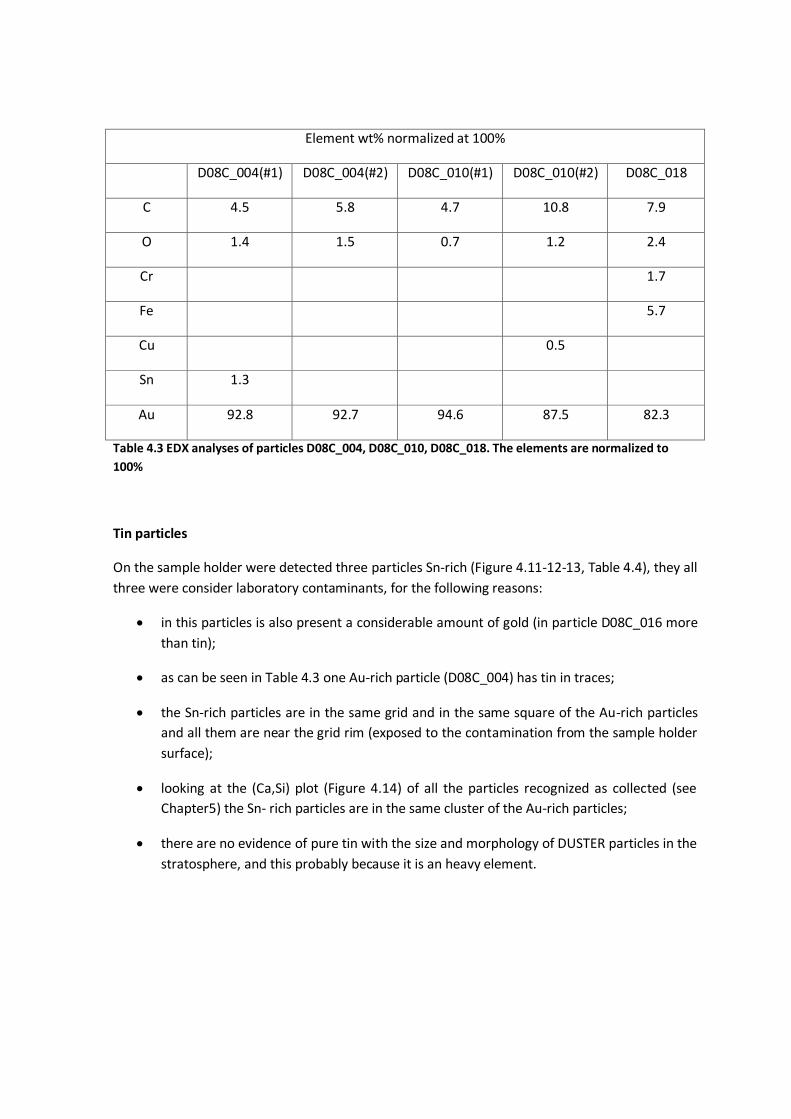
Element wt% normalized at 100%
D08C_004(#1) D08C_004(#2) D08C_010(#1) D08C_010(#2) D08C_018
C 4.5 5.8 4.7 10.8 7.9
O 1.4 1.5 0.7 1.2 2.4
Cr 1.7
Fe 5.7
Cu 0.5
Sn 1.3
Au 92.8 92.7 94.6 87.5 82.3
Table 4.3 EDX analyses of particles D08C_004, D08C_010, D08C_018. The elements are normalized to
100%
Tin particles
On the sample holder were detected three particles Sn-rich (Figure 4.11-12-13, Table 4.4), they all
three were consider laboratory contaminants, for the following reasons:
in this particles is also present a considerable amount of gold (in particle D08C_016 more
than tin);
as can be seen in Table 4.3 one Au-rich particle (D08C_004) has tin in traces;
the Sn-rich particles are in the same grid and in the same square of the Au-rich particles
and all them are near the grid rim (exposed to the contamination from the sample holder
surface);
looking at the (Ca,Si) plot (Figure 4.14) of all the particles recognized as collected (see
Chapter5) the Sn- rich particles are in the same cluster of the Au-rich particles;
there are no evidence of pure tin with the size and morphology of DUSTER particles in the
stratosphere, and this probably because it is an heavy element.
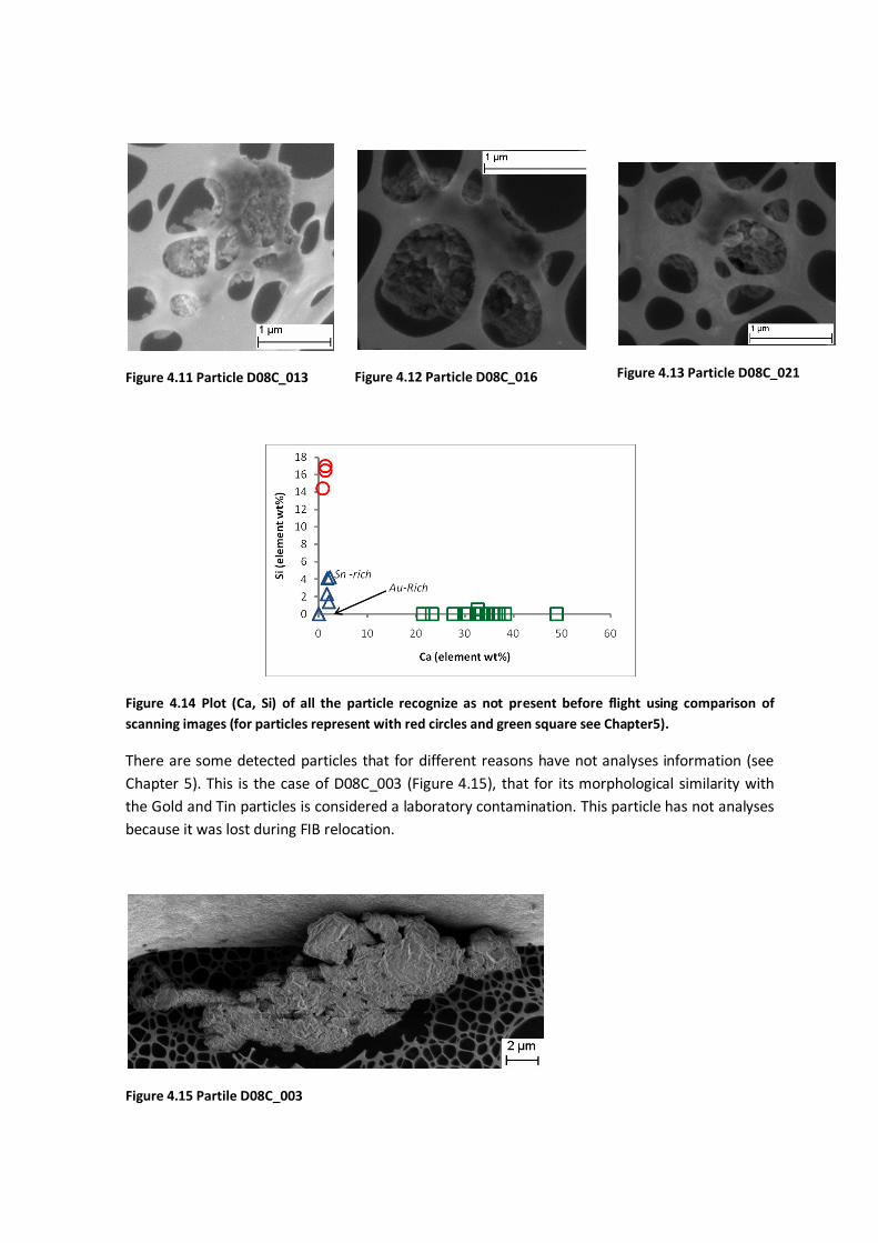
Figure 4.11 Particle D08C_013
Figure 4.14 Plot (Ca, Si) of all the particle recognize as not present before flight using comparison of
scanning images (for particles represent with red circles and green square see Chapter5).
There are some detected particles that for different reasons have not analyses information (see
Chapter 5). This is the case of D08C_003 (Figure 4.15), that for its morphological similarity with
the Gold and Tin particles is considered a laboratory contamination. This particle has not analyses
because it was lost during FIB relocation.
Figure 4.15 Partile D08C_003
Figure 4.12 Particle D08C_016
Figure 4.13 Particle D08C_021

Element wt% contamination corrected
D08C_013 (#1) D08C_013 (#2) D08C_016 D08C_020
C 26.6 26.4 32.5 21.8
O 23.0 23.3 24.2 17.2
Na 0.6 1.0
Al 0.6 0.6
Si 1.2 1.9 3.3 3.6
Ca 1.7 1.4 1.4 2.0
Fe 18.5
Cu 3.5
Zn 2.1
Sn 27.1 29.0 14.3 22.3
Au 18.3 17.4 19.2 14.0
Table 4.4 EDX analyses of particles D08C_013, D08C_016, D08C_020. The elements are normalized to
100% after Fe, Cr, Ni correction
4.3.2 Source of contamination by FIB
As mentioned in Chapter 3, the particles relocated with FIB instrument are fixed in a copper grid,
the needle used to relocate them is made of tungsten and the sealing and unsealing is made with
platinum and gallium respectively. So the particles relocated with FIB could be contaminated with
Cu, Pt, Ga, and W. Also in this case the problem of contamination is solved subtracting the
contaminant elements and normalizing the remnants elements to 100%.
In the Table 4.5 is shown an example of particle relocated with FIB. The particle in the DUSTER
collector looks like a single particle, but in reality it was composed of two particles. The first thing
notable is that D08C_008b has a composition similar to the EDX bulk analyses of almost all the
particle (D08C_008) performed when the particle was still on the DUSTER collector. However,
D08C_008a is different. A subsequent Raman analysis of D08C_008a and D08C_008b shown that
in the particles and in the copper grid where they are sealed there is the amorphous carbon
feature (see Chapter 5). All the evidences above let suppose that the FIB instrument is a also a
source of contamination for sub-micron size amorphous carbon particles too.

Element wt% of the same particle before and after relocation with FIB instrument
D08C_008 D08C_008a D08C_008b
C 24.8 66.4 22.3 O 39.2 24.0 37.8
Na 0.4 1.2
Mg 0.2 Al 1.5 4.4
Si 1.2
S 1.0
Cl 1.7 K 1.1
Ca 34.5 1.7 35.5
Fe 1.1 Table 4.5 Example of particle (D08C_008) relocated with FIB instrument. After relocation the particle
divided into two different parts (D08C_008a and D08C_008b). The analyses reported in the table are EDX
analyses contamination corrected and normalized to 100%. The D08C_008a in Raman analyses has a-C,
the particle D08C_008b has a-C and calcite. The EDX spectrum of D08C_008b is more similar to the
D08C_008 than the D08C_008a.
4.3.3 Sources of contamination from the flight train
In the flight train of the DUSTER collector has above it, in a range of almost 20 m: a balloon, a
parachute, 4 solar panels and a telemetry package. All these objects can be potential sources of
contamination being exposed to the external environment for all the time from the preparation of
the launch to the end of collection. It is not possible to exclude contamination from the flight
train, but we can be confident that there is a low probability of contamination from these sources
for the following reasons:
1. the particles in the nanometer/micrometer range remain attached to the objects were
they are deposit thanks to the Van der Waals forces;
2. the particles deposit on the balloon surface are not ejected because of the difference of
pressure that blow up the balloon because the decreasing of pressure with altitude was
constant and not sudden (Figure 4.16);
3. the inlet tube remain closed until the altitude of ~25 km when the pressure inside the
inlet equal the external pressure and the flange that seal the inlet falls down;
4. the valve that open the collecting chamber is opened at ~35 km, and the pressure inside
the chamber is higher than outside, so the first air flux is directed outside the chamber. If
there is something deposit in the inlet is not aspired but pushed out.

Figure 4.16 Plot of changing of pressure with altitude. From down to up the ascendant phase (during
which the balloon blow up), the floating phase (during which the balloon has almost a constant volume)
and the descendent time (the instrument is free from the balloon).
Conclusions
Even when the procedures to preserve clean the sample holders were correctly followed, on the
collection surface were found contamination almost all due to the sample holder itself. The
contamination problem is solved for DUSTER2008 campaign by not considering all the particles
that are sources of ambiguity and removing the chemical elements due to substrate. The problem
of contamination due to the sample holder structure and materials is definitively solved changing
the structure for the DUSTER 2009 campaign (see Chapter 6).
Also the problems due to the scanning procedures were solved for DUSTER 2009 campaign, but in
DUSTER 2008 collection the lost of information fixed a cut-off in size and number of particles that
could be identified as collected. For example all the particles less than 0.5 µm are too little to be
detected from the resolution of our scanning.
In the end trying to relocate the particles with FIB instrument it is clear that this kind of
technology is not useful for particles <20 µm; the range is established by the particles collected
and relocated with FIB, we have not information on what happened for particles > 20 µm. For
particles less than 5 µm the FIB technique causes the loss of part of the particle’s mass and the
presence of contamination due to the tools used to relocate samples. For particles less than 5 µm
the particle’s mass lost after relocation is almost 50% and the remnant is totally embedded in
contamination elements. For this reasons I can conclude that FIB technology is not useful to
handle the particles in the size range less than 20 µm for the DUSTER experiment.

5 Sample collected during the June 2008
campaign: analyses results
In this chapter are shown the results of DUSTER 2008 flight:
the particles are classified by size, morphological class and composition;
it is reported a catalogue of raw data of chemical analyses (FESEM-EDX, FT-IR and Raman
spectroscopy);
are discussed the origins of contaminants element and how to remove it;
finally there is a discussion of data reduction and the origins of collected particles.

5.1 Particle statistics and size distribution
DUSTER flew from Svalbard to Greenland (Figure 2.3) and collected particles at an average
altitude of 37 km during a 55h period during June 2008.
The scanning procedure performed by FESEM on the collector led to the identification of 32
particles as present only post-flight. Among the 32 identified particles, 7 are classified as
laboratory contamination (cf. Chapter 4) and 25 as collected stratospheric particles. In this
chapter only the 25 stratospheric particles will be considered.
As discussed on the previous chapter, not all the collecting areas were examined. The procedure
of comparison between pre- and post-flight FESEM scanning to recognize the collected particles
was limited to 12 grids instead of 14. Grids 5 and 6 were not scanned pre-flight. Particles > 100
µm when placed in the FESEM electron beam using at EHT (Extra High Tension) = 10 kV (the
voltage used to scan the grids) are at risk of charging causing them to jump away; in order to not
lose the spheres (100 – 150 µm size) the grids wherein they are located were not scanned during
post-flight analysis. For this reason the comparison for grids 4 and 9 (where the spheres are
collected) was done looking at the grids in real time with FE-SEM and using pre-flight images to
check the particles identified.
Each TEM grid has roughly 500 mesh (metal squares that compose the grid), it means a total of
5000 mesh for 10 grids. Because of the pin structure (see Chapter4) before the flight there was
148/5000 mesh damage, that after flight became 1074/5000 probably due to thermal shock.
Finally the Collector’s area investigated to search for particles collected in stratosphere is less
than 50 % of the whole collector and consequently the number of collected particles might be
higher. The distribution of particles is shown in (Table 5.1), the majority is in the ‘central grid’ and
neighboring grids, but this is not statistically relevant because those are the grids with the high
resolution scanning (see Chapter 4).
‘central grid’ 12 particles
Grids 1 and 2 (1 particle each grid) 2 particle
grid 7 3 particles
grids 4, ‘9, 10’, 11, 12 and 13 (one each grid) 6 particles
grids 8 2 particles
Table 5.1 Numbers of stratospheric particles collected in the investigated grids.

The size of each collected particle was measured (µm) by a FESEM tool. For particles that are not
perfect spheres were measured the minimum (a) and maximum (b) dimension and calculated the
equivalent size using the quadratic mean (Table 5.2) of the two measures:
2
22 baSize
The aspect ratio a/b gives an estimate of the particle’s degree of roundness (Figure 5.2), if it is 1
the particle is a disk or a sphere, if it is about 0 it is similar to a hourglass or a needle. Examining
the collected particle size distribution it is evident that more than 90% of them are in the size
range (0.5 – 7) µm (Figure 5.1), according to the instrument requirements and that except for the
particles > 100 µm (they are spherical) the particles identified as collected are in the range of
ellipsoidal shape (Figure 5.3).
Figure 5.1 Size distribution of the 25 stratospheric particles collected
Figure 5.2 Plot size vs aspect ratio of the 25 stratospheric particles collected. The two circles represent the
spheres.

Particle a b a/b equivalent size
D08C_001 140.70 140.70 1 140.70
D08C_002 116.30 116.30 1 116.30
D08C_005 4.40 8.18 0.5 6.60
D08C_006 5.84 7.75 0.75 6.85
D08C_007 6.10 6.64 0.9 6.40
D08C_008 3.88 8.50 0.5 6.60
D08C_009 3.86 5.41 0.7 4.70
D08C_011 1.60 3.40 0.5 2.65
D08C_012 1.65 3.10 0.5 2.50
D08C_014 1.85 2.96 0.6 2.40
D08C_015 1.41 2.35 0.6 1.95
D08C_017 0.50 1.85 0.2 1.35
D08C_019 1.00 1.31 0.75 1.20
D08C_021 1.42 1.47 0.8 1.60
D08C_022 0.60 1.29 0.5 1.00
D08C_023 0.86 1.66 0.5 1.30
D08C_024 1.15 1.35 0.85 1.25
D08C_025 0.66 1.00 0.7 0.85
D08C_026 0.47 0.90 0.5 0.70
D08C_027 0.49 0.86 0.6 0.70
D08C_028 0.44 1.07 0.4 0.80
D08C_029 0.54 0.87 0.6 0.70
D08C_030 0.47 0.84 0.6 0.70
D08C_031 0.45 0.56 0.8 0.50
D08C_032 0.42 0.52 0.8 0.45
Table 5.2 In this table are reported the minimum (a) and maximum (b) elongation, the level of roundness
(a/b) and the equivalent size ( sqrt[(a2+b2)/2]) of the 25 stratospheric particles collected.
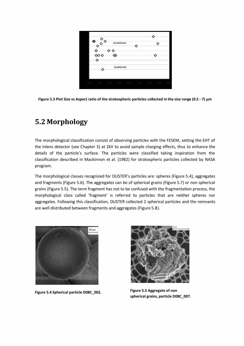
Figure 5.3 Plot Size vs Aspect ratio of the stratospheric particles collected in the size range (0.5 - 7) µm
5.2 Morphology
The morphological classification consist of observing particles with the FESEM, setting the EHT of
the Inlens detector (see Chapter 3) at 2kV to avoid sample charging effects, thus to enhance the
details of the particle’s surface. The particles were classified taking inspiration from the
classification described in Mackinnon et al. (1982) for stratospheric particles collected by NASA
program.
The morphological classes recognized for DUSTER’s particles are: spheres (Figure 5.4), aggregates
and fragments (Figure 5.6). The aggregates can be of spherical grains (Figure 5.7) or non spherical
grains (Figure 5.5). The term fragment has not to be confused with the fragmentation process, the
morphological class called ‘fragment’ is referred to particles that are neither spheres nor
aggregates. Following this classification, DUSTER collected 2 spherical particles and the remnants
are well distributed between fragments and aggregates (Figure 5.8).
Figure 5.4 Spherical particle D08C_002.
Figure 5.5 Aggregate of non
spherical grains, particle D08C_007.

Figure 5.6 Fragment, particle D08C_009.
Figure 5.8 In the plot are represented the morphological groups in function of size. The red diamonds are
the fragments, the light blue diamonds are the aggregates of non spherical grains, the purple diamonds
are the particles defined as fragment/aggregates, and the green diamonds are the aggregate of spherical
grains.
5.3 Catalogue of raw data
Here following I will present the particle’s catalogue with the relative results obtained with the
different analytical techniques applied.
For each of the 25 particles collected is shown:
FE-SEM image (where they are necessary to highlight particular morphological features,
there are more images);
EDX analyses (without contamination removal);
size (µm);
morphological class;
Figure 5.7 Aggregate of spherical
grains, particle D08C_031.

composition;
position on the sample holder.
For some of the 25 particles we do not have information about composition. They are moved in a
particular section at the end of the catalogue, called ‘Particles Unknown’.

D08C_001
Figure 5.9 FESEM image at 2 kV of particle D08C_001
The surface is mainly smooth but there are pits, projections and fractures.
Looking at the mosaic of pictures taken by FE-SEM going into high magnification (Figure 5.10) are
visible structures that seems to come up from the surface or be under surface. There are also
(unidentified) fragments that seems to be extraneous to the sphere attached on the surface.
Pieces of holey carbon film, detached from the TEM grid, are visible on the sphere’s surface.
Looking at the sphere with an optical microscope are visible bubbles inside (Figure 5.11) it show
also that the sphere is transparent.
Figure 5.10 Mosaic of particulars of particle D08C_001 performed with FESEM at 2 kV.
Size: 140.70 µm
Position: grid 9
Morphological class: Sphere
Composition: O, Si, Na, C, Ca, Mg, Fe, Al
Analyses Performed:
FESEM-EDX

Figure 5.11 Picture of the particle D08C_001 on a substrate of KBr. The white spots are reflection of the
light of the microscope on the particle. Is also visible near the center little bubbles of different size. On
the external part can be see residual of carbon film.
EDX ( 15kV) bulk analysis
Elements Weight % Sigma
O 62.92 0.50
Na 9.24 0.17
Mg 2.03 0.09
Al 0.16 0.06
Si 22.97 0.19
Ca 2.55 0.10
Fe 0.47 0.12
Au 5.43 0.34
TOT 105.77
Table 5.3 EDX analysis of the area shown in Figure 5.12
Figure 5.12 Area of the particle in which is performed the
EDX

EDX (15kV) spot analysis
Elements Weight % Sigma
C 6.62 0.45
O 63.60 0.51
Na 6.27 0.15
Mg 1.59 0.08
Al 0.20 0.06
Si 18.35 0.17
Ca 1.57 0.08
Au 4.73 0.32
TOT 102.93
Table 5.4 EDX analysis of the area shown in Figure 5.13
Figure 5.13 Area of the particle in which is performed the
EDX

D08C_002
Figure 5.14 FESEM image at 2 kV of particle D08C_002
As in the previous case (D08C_001) the sphere is not so smooth as it appears looking at the Figure
5.14. Going into high magnifications also in this case are visible pits, fractures and fragments
attached on the surface (Figure 5.15).
During relocation this particle was lost, but in Figure 5.16 there is a picture of the particle on the
DUSTER sample holder performed with the optical microscope and it is transparent and with
bubble inside. The bubbles show a size gradient from the smaller (near the center) to the largest
(near the surface).
Figure 5.15 Mosaic of particulars of particle D08C_002 performed with FESEM at 2 kV.
Size: 116.30 µm
Position: grid 4
Morphological class: Sphere
Composition: O, Si, C, Na, Ca, Mg, Al
Analyses Performed:
FESEM-EDX

Figure 5.16 Picture of the particle D08C_002 on the DUSTER sample holder. The white spots are reflection
of the light of the microscope on the particle. Is also visible on left side a big bubble and on right side
bubbles of different size. In this picture is also evident that the particle is transparent.
EDX (15 kV) bulk analysis
Elements Weight % Sigma
C 7.65 0.45
O 53.50 0.50
Na 7.28 0.15
Mg 1.68 0.08
Al 0.16 0.06
Si 19.39 0.18
Ca 2.10 0.09
Au 3.55 0.28
TOT 95.31
Table 5.5 EDX analysis of the area shown in
Figure 5.17
Figure 5.17 Area of the particle in which is performed the
EDX

D08C_006
Figure 5.18 FESEM image at 2 kV of particle
D08C_006
EDX (10 kV) spot analysis
Element Weight % Sigma
C 14.13 0.12
O 52.73 0.52
Ca 35.78 0.44
Au 4.71 0.48
TOT 107.35
Table 5.6 EDX analysis of the area shown in Figure 5.19
Size: 6.85 µm
Position: central grid
Morphological class: Aggregate of non spherical grains
Composition: O, Ca, C
Analyses Performed:
FESEM-EDX
Relocated using FIB instrument
Raman
Figure 5.19 Area of the particle in which is performed
the EDX
Figure 5.20 Area of the particle in which is performed
the EDX
EDX (15 kV) spot analysis
Element Weight % Sigma
C 13.79 0.15
O 14.14 0.43
F 1.24 0.29
Al 2.03 0.11
Ca 29.76 0.30
Cu 24.05 0.47
Pt 8.57 0.38
TOT 93.58
Table 5.7 EDX analysis of the area shown in Figure
5.20
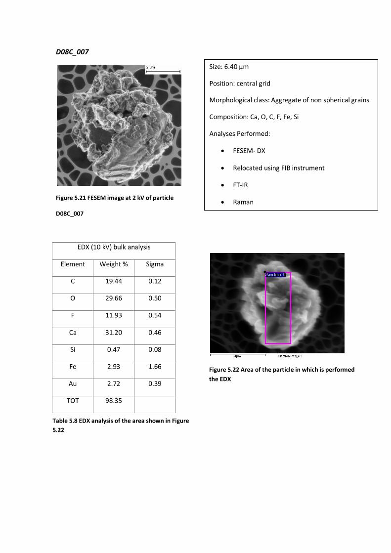
D08C_007
Figure 5.21 FESEM image at 2 kV of particle
D08C_007
EDX (10 kV) bulk analysis
Element Weight % Sigma
C 19.44 0.12
O 29.66 0.50
F 11.93 0.54
Ca 31.20 0.46
Si 0.47 0.08
Fe 2.93 1.66
Au 2.72 0.39
TOT 98.35
Table 5.8 EDX analysis of the area shown in Figure
5.22
Size: 6.40 µm
Position: central grid
Morphological class: Aggregate of non spherical grains
Composition: Ca, O, C, F, Fe, Si
Analyses Performed:
FESEM- DX
Relocated using FIB instrument
FT-IR
Raman
Figure 5.22 Area of the particle in which is performed
the EDX

D08C_008
Figure 5.23 FESEM image at 2 kV of particle
D08C_008
On DUSTER collector it seems to be a single particle compose of a fragment and some little grains
attached on it. During FIB relocation was clear that actually it is an optical effect. There are two
particles very close one to each other.
They were renamed D08C_008(a) (the biggest fragment) and D08C_008(b) (the smallest
fragment). The EDX reports above is in a bulk region that takes in account both the fragments. In
order to have an EDX for each single fragment, after relocation it was performed a new EDX
analysis for each of the two particles.
EDX (15 kV) bulk analysis
Element Weight % Sigma
C 16.30 0.12
O 25.75 0.39
Na 0.24 0.06
Ca 22.62 0.23
Fe 0.71 0.16
Au 48.52 0.57
TOT 114.14
Table 5.9 EDX analysis of the area shown in Figure 5.24
Size: 6.60 µm
Position: central grid
Morphological class: Aggregate of non spherical grains
Composition: O, Ca, C, Fe, Na
Analyses Performed:
FESEM-EDX
Relocated using FIB instrument
FT-IR
Raman
Figure 5.24 Area of the particle in which is performed
the EDX

D08C_008(b)
D08C_008(a)
EDX (15 kV) bulk analysis
Element Weight % Sigma
C 17.12 0.14
O 29.04 0.47
Al 3.38 0.11
Ca 27.28 0.25
Cu 16.91 0.36
Pt 7.92 0.31
TOT 101.65
Table 5.10 EDX analysis of the area shown in Figure 5.25
EDX (15 kV) bulk analysis
Element Weight % Sigma
C 62.23 0.66
O 22.55 0.43
Na 1.11 0.09
Mg 0.19 0.06
Al 1.37 0.08
Si 1.12 0.06
S 0.96 0.09
Cl 1.6 0.07
K 1.02 0.08
Ca 1.75 0.10
Cu 2.78 0.26
TOT 96.68
Table 5.11 EDX analysis of the area shown in Figure 5.26
Figure 5.25 Area of the particle in which is performed
the EDX
Figure 5.26 Area of the particle in which is performed
the EDX

D08C_009
Figure 5.27 Image at 2 kV of particle D08C_009
EDX (10 kV) bulk analysis
Element Weight % Sigma
C 15.35 0.11
O 47.12 0.55
F 2.33 0.36
Ca 26.95 0.44
Au 9.2 0.53
TOT 100.95
Table 5.12 EDX analysis of the area shown in Figure 5.28
Size: 4.70 µm
Position: central grid
Morphological class: Fragment
Composition: O, Ca, C, F
Analyses Performed:
FESEM-EDX
Relocated using FIB instrument
FT-IR
Figure 5.28 Area of the particle in which is performed
the EDX
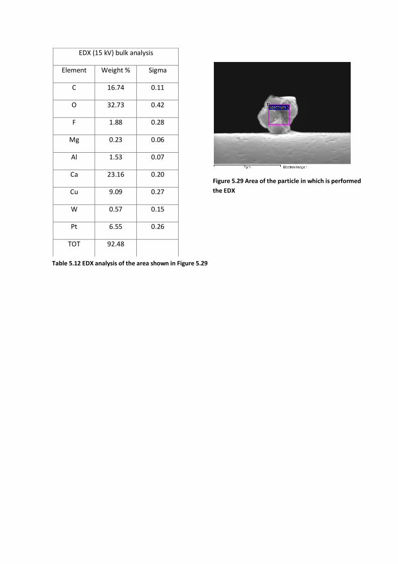
EDX (15 kV) bulk analysis
Element Weight % Sigma
C 16.74 0.11
O 32.73 0.42
F 1.88 0.28
Mg 0.23 0.06
Al 1.53 0.07
Ca 23.16 0.20
Cu 9.09 0.27
W 0.57 0.15
Pt 6.55 0.26
TOT 92.48
Table 5.12 EDX analysis of the area shown in Figure 5.29
Figure 5.29 Area of the particle in which is performed
the EDX

D08C_011
Figure 5.30 Image at 2 kV of particle D08C_011
EDX (10 kV) bulk analysis
Element Weight % Sigma
C 4.41 0.51
O 10.94 0.28
Na 0.42 0.12
Al 2.55 0.11
Si 2.92 0.12
P 0.48 0.12
K 0.98 0.12
Cr 11.87 3.05
Fe 43.86 1.31
Ni 5.95 0.59
TOT 84.38
Table 5.13 EDX analysis of the area shown in Figure 5.31
Size: 2.65 µm
Position: grid 1
Morphological class: Fragment
Composition: O, C, Si, Al, K, P, Na
Analyses Performed:
FESEM-EDX
Figure 5.31 Area of the particle in which is performed
the EDX

EDX (10 kV) spot analysis
Element Weight % Sigma
C 4.74 0.50
O 10.64 0.27
Na 0.47 0.12
Al 2.21 0.11
Si 2.96 0.12
P 0.52 0.12
K 0.26 0.12
Cr 12.53 3.01
Fe 45.95 1.34
Ni 6.08 0.61
TOT 83.36
Table 5.14 EDX analysis of the area shown in Figure 5.32
Figure 5.32 Area of the particle in which is performed
the EDX

D08C_012
Figure 5.33 Image at 2 kV of particle D08C_012
Figure 5.35 Area in which is performed the EDX
EDX (10 kV) spot analysis
Element Weight % Sigma
C 13.76 0.31
O 32.14 0.50
F 1.17 0.25
Mg 0.25 0.07
Ca 27.67 0.42
Au 27.84 0.79
TOT 102.83
Table 5.15 EDX analysis of the area shown in Figure 5.34
Size: 2.50 μm
Position: central grid
Morphological class: Fragment/Aggregate
Composition: O, Ca, C, F, Mg
Analyses Performed:
FESEM-EDX
Figure 5.34 Area of the particle in which is performed
the EDX
EDX (10 kV) spot analysis
Element Weight % Sigma
C 18.88 0.34
O 54.29 0.64
Mg 0.29 0.08
Ca 35.41 0.47
Au 10.04 0.59
TOT 118.91
Table 5.16 EDX analysis of the area shown in Figure
5.35

EDX (10 kV) bulk analysis
Element Weight % Sigma
C 15.46 0.33
O 44.91 0.58
Ca 30.34 0.44
Au 23.13 0.74
TOT 113.84
Table 5.17 EDX analysis of the area shown in
Figure 5.36
Figure 5.36 Area of the particle in which is performed
the EDX

D08C_015
Figure 5.37 Image at 2 kV of particle D08C_015
EDX (10 kV) bulk analysis
Element Weight % Sigma
C 16.94 0.40
O 29.90 0.47
F 1.46 0.31
Ca 14.69 0.34
Au 71.67 1.12
TOT 134.66
Table 5.18 EDX analysis of the area shown in Figure 5.38
EDX (10 kV) spot analysis
Element Weight % Sigma
C 16.80 0.36
O 44.01 0.57
Mg 0.28 0.09
Ca 29.62 0.43
Au 38.99 0.92
TOT 129.70
Table 5.19 analysis of the area shown in Figure 5.39
Size: 1.95 μm
Position: central grid
Morphological class: Fragment
Composition: O, Ca, C, F, Mg
Analyses Performed:
FESEM-EDX
Figure 5.39 Area of the particle in which is performed
the EDX
Figure 5.38 Area of the particle in which is performed
the EDX

D08C_019
Figure 5.40 Image at 2 kV of particle D08C_019
Table5.20 EDX analysis of the area shown in Figure 5.41
Figure 5.42 Area of the particle in which is performed the EDX
EDX (10 kV) spot analysis
Element Weight % Sigma
C 14.97 0.33
O 32.12 0.51
Ca 26.27 0.39
Cr 13.29 5.38
Ni 2.09 0.45
Fe 27.00 1.35
TOT 115.74
Size: 1.20 μm
Position: central grid
Morphological class: Fragment/Aggregate
Composition: O, Ca, C, P, Na
Analyses Performed:
FESEM-EDX
Figure 5.41 Area of the particle in which is performed the
EDX
EDX (10 kV) bulk analysis
Element Weight % Sigma
C 15.16 0.34
O 29.00 0.48
Na 0.39 0.11
P 0.47 0.13
Ca 24.05 0.38
Cr 15.20 5.01
Ni 2.38 0.47
Fe 31.74 1.39
Au 1.61 0.50
TOT 120.00
Table 5.21 EDX analysis of the area shown in Figure
5.42

D08C_021
Figure 5.43 Image at 2 kV of particle D08C_021
EDX (10 kV) bulk analysis
Element Weight % Sigma
C 12.75 0.30
O 38.48 0.55
F 1.07 0.31
Ca 29.97 0.43
Au 18.98 0.70
TOT 101.25
Table 5.22 EDX analysis of the area shown in Figure 5.44
Size: 1.60 μm
Position: central grid
Morphological class: Fragment
Composition: O, Ca, C, F
Analyses Performed:
FESEM-EDX
Figure 5.44 Area of the particle in which is performed
the EDX

D08C_022
Figure 5.45 Image at 2 kV of particle D08C_022
EDX (10 kV) spot analysis
Element Weight % Sigma
C 5.30 0.29
O 4.78 0.24
Si 0.52 0.09
Cr 13.94 2.56
Fe 58.73 1.44
Ni 14.53 0.74
Au 4.49 0.52
TOT 102.29
Table 5.23 EDX analysis of the area shown in Figure 5.46
Size: 0.95 μm
Position: grid 7
Morphological class: Fragment
Composition: C, O
Analyses Performed:
FESEM-EDX
Figure 5.46 Area of the particle in which is performed
the EDX

D08C_023
Figure 5.47 Image at 2 kV of particle D08C_023
Figure 5.49 Area in which is performed the EDX
EDX (10 kV) bulk analysis
Element Weight % Sigma
C 7.31 0.33
O 4.28 0.27
Na 0.70 0.14
Si 0.38 0.10
Ca 1.02 0.16
Cr 21.56 2.80
Fe 74.67 1.64
Ni 10.97 0.79
Zr 1.43 0.38
TOT 122.32
Table 5.24 EDX analysis of the area shown in Figure 5.48
Size: 1.30 μm
Position: central grid
Morphological class: Aggregate of non-spherical
grains
Composition: C, O, Ca, Na
Analyses Performed:
FESEM-EDX
Figure 5.48 Area of the particle in which is performed
the EDX
EDX (10 kV) bulk analysis
Element Weight % Sigma
C 7.75 0.31
O 3.75 0.25
Na 0.79 0.14
Si 0.29 0.10
P 0.58 0.13
Cr 16.49 2.58
Fe 70.81 1.54
Ni 11.98 0.76
TOT 112.44
Table 5.25 EDX analysis of the area shown in Figure
5.49

D08C_025
Figure 5.50 Image at 2 kV of particle D08C_025
EDX (10 kV) bulk analysis
Element Weight % Sigma
C 21.27 0.43
O 8.64 0.30
Si 0.35 0.08
Cr 17.45 3.10
Fe 61.09 1.55
Ni 9.68 0.69
Au 5.24 0.50
TOT 123.72
Table 5.26 EDX analysis of the area shown in Figure 5.51
Size: 0.85 μm
Position: grid 7
Morphological class: Aggregate of non-spherical
grains
Composition: C, O
Analyses Performed:
FESEM-EDX
Figure 5.51 Area of the particle in which is performed
the EDX

D08C_026
Figure 5.52 Image at 2 kV of particle D08C_026
EDX (10 kV) bulk analysis
Element Weight % Sigma
C 5.12 0.27
O 3.97 0.24
Na 0.46 0.14
Si 0.27 0.09
P 0.69 0.13
Cr 16.08 2.49
Fe 63.26 1.47
Ni 8.58 0.73
TOT 98.43
Table 5.27 EDX analysis of the area shown in Figure 5.53
Size: 0.70 μm
Position: grid 8
Morphological class: Aggregate of non-spherical
grains
Composition: C, O, Na
Analyses Performed:
FESEM-EDX
Figure 5.53 Area of the particle in which is performed
the EDX

D08C_027
Figure 5.54 Image at 2 kV of particle D08C_027
EDX (15 kV) spot analysis
Element Weight % Sigma
C 8.20 0.37
O 1.75 0.25
Cr 0.96 0.14
Fe 2.70 0.20
Cu 0.49 0.30
Au 78.14 0.72
TOT 92.24
Table 5.28 EDX analysis of the area shown in Figure 5.55
Size: 0.70 μm
Position: grid 7
Morphological class: Aggregate of non-spherical
grains
Composition: C, O
Analyses Performed:
FESEM-EDX
Figure 5.55 Area of the particle in which is performed
the EDX

D08C_028
Figure 5.56 Image at 2 kV of particle D08C_028
EDX (15 kV) bulk analysis
Element Weight % Sigma
C 15.44 0.42
O 12.23 0.36
Na 0.50 0.13
Si 0.31 0.07
Ca 4.37 0.12
Cr 14.85 0.25
Fe 51.33 0.51
Ni 5.31 0.32
Au 2.75 0.36
TOT 107.09
Table 5.29 EDX analysis of the area shown in Figure 5.57
Size: 0.80 μm
Position: central grid
Morphological class: Aggregate of non-spherical
grains
Composition: C, O, Na
Analyses Performed:
FESEM-EDX
Figure 5.57 Area of the particle in which is performed
the EDX

D08C_029
Figure 5.58 Image at 2 kV of particle D08C_029
Figure 5.60 Area of the particle in which is performed
the EDX
EDX (10 kV) spot analysis
Element Weight % Sigma
C 10.16 0.34
O 2.34 0.25
Si 0.32 0.09
Cr 18.25 2.55
Fe 69.74 1.56
Ni 10.70 0.78
TOT 111.51
Table 5.30 EDX analysis of the area shown in Figure 5.59
Size: 0.70 μm
Position: grid 11
Morphological class: Plate aggregate with a
spherical grain
Composition: C, O
Analyses Performed:
FESEM-EDX
Figure 5.59 Area of the particle in which is performed
the EDX
EDX (15 kV) spot analysis
Element Weight % Sigma
C 45.46 0.58
O 5.74 0.37
Si 0.33 0.06
Cr 13.15 0.24
Fe 48.77 0.51
Ni 5.76 0.31
Au 1.84 0.32
TOT 121.05
Table 5.31 EDX analysis of the area shown in Figure
5.60

D08C_030
Figure 5.61 Image at 2 kV of particle D08C_030
EDX (10 kV) bulk analysis
Element Weight % Sigma
C 45.52 0.53
O 6.29 0.32
Na 0.45 0.11
Si 0.27 0.08
Cr 12.52 3.07
Fe 39.32 1.31
Ni 4.12 0.50
Au 6.86 0.55
TOT 115.35
Table 5.32 EDX analysis of the area shown in Figure 5.62
Size: 0.70 μm
Position: grid 8
Morphological class: Fragment
Composition: C, O, Na
Analyses Performed:
FESEM-EDX
Figure 5.62 Area of the particle in which is performed
the EDX

D08C_031
Figure 5.63 Image at 2 kV of particle D08C_031
EDX (10 kV) bulk analysis
Element Weight % Sigma
C 6.35 0.29
O 10.59 0.28
Si 0.25 0.08
Cr 12.63 3.07
Fe 64.33 1.47
Ni 5.43 0.61
Au 4.54 0.48
TOT 104.12
Table 5.33 EDX analysis of the area shown in Figure 5.64
Size: 0.50 μm
Position: central grid
Morphological class: Aggregate of spherical
grains
Composition: C, O
Analyses Performed:
FESEM-EDX
Figure 5.64 Area of the particle in which is performed
the EDX

D08C_032
Figure 5.65 Image at 2 kV of particle D08C_032
EDX (10 kV) spot analysis
Element Weight % Sigma
C 9.15 0.30
O 11.18 0.27
Na 0.23 0.10
Si 0.26 0.07
Cr 15.60 2.89
Fe 50.58 1.36
Ni 7.29 0.60
Au 2.70 0.41
TOT 96.99
Table 5.34 EDX analysis of the area shown in Figure 5.66
Size: 0.45 μm
Position: grid 2
Morphological class: Fragment
Composition: C, O, Na
Analyses Performed:
FESEM-EDX
Figure 5.66 Area of the particle in which is performed
the EDX

Particles of unknown composition
The particles present in this catalogue are particles for which there are not compositional
analyses and they are now lost or relocated. In the case they are relocated they lost to much mass
to allow EDX analyses.
D08C_005
Figure 5.67 Image at 10 kV of particle D08C_005
During EDX analyses the biggest part of the particle disappeared (may be evaporated) by the
interaction with the electron beam. It seems to be some kind of membrane that encapsulating
many small grains, but noting remained after analysis except for a 3.20 µm aggregate of non
spherical grains. This behavior let suppose that the membrane was made of light elements, such
as some kind of hydrocarbons.
Figure 5.68 Image at 2 kV of particle D08C_005 after EDX analysis
To avoid that this residual will evaporate, no analyses ware performed before relocation. But after
relocation it seems to be smaller than before and completely embedded in FIB tools elements
(Figure 5.69).
Size: 6.60 µm
Position: central grid
Morphological class: Aggregate of non-spherical grains
Analyses Performed:
FESEM-EDX
Relocated using FIB instrument
Figure 5.69 Image at 2 kV of particle
D08C_005 relocated

D08C_014
Figure 5.70 Image at 2 kV of particle D08C_014
The EDX analysis was done without a calibration standard. The un-calibrated analysis data show
the presence of: O, C, Cr, Fe, Ni and Au.
After relocation it was sent to another laboratory (no data are available as yet).
D08C_017
Figure 5.71 Image at 2 kV of particle D08C_017
The EDX analysis was done without a calibration standard. The un-calibrated analysis data shows
the presence of C, O, Si, Cr, Mn, Fe, Ni, Au.
During relocation the particle was charged and jumped away, we lost it.
Size: 2.40 μm
Position: grid 10
Morphological class: Fragment
Analyses Performed:
FESEM-EDX
Relocated using FIB instrument
FT-IR
Size: 1.35 μm
Position: grid 13
Morphological class: Aggregate of mostly non-
spherical grains
Analyses Performed:
FESEM-EDX
Relocation using FIB instrument

D08C_024
Figure 5.72 Image at 2 kV of particle D08C_024
The EDX analysis was done without a calibration standard. The un-calibrated EDX data show the
presence of: C, O, Cr, Fe, Ni and Au.
The particle was relocated (Figure 5.73) before to do a calibrated analysis (no data are available as
yet).
Figure 5.73 Image at 2 kV of particle D08C_024 after relocation
Size: 1.25 μm
Position: grid 12
Morphological class: Aggregate of non-spherical
grains
Analyses Performed:
FESEM
EDX
Relocated using FIB instrument

5.4 Data reduction
The data reduction involve the following steps:
1. remove the contribution of contaminant elements. As previously discussed in Chapter 4
each particle with a major contribution of gold is removed from the dataset because they
are contaminant particles. In the cases where there are Cr, Fe and Ni in the same analysis
the grains are removed as contribution of pin substrate. If there are the minor elements
of the stainless steel composition (C, O, Si, P and S) they are removed only when these
elements occur proportionally with the Fe-ratios in the stainless steel composition (Figure
4.7).
2. normalization of EDX data. Looking at the raw data is evident that EDX total is never
100%. It can be more than 100% (probably due to the charge of particle during analyses)
or can be less than 100% (due elements undetectable by FESEM-EDX instrument , such as
hydrogen);
3. oxide calculation using EDX data;
4. comparison of EDX analyses with FT-IR (Figure 5.74) and Raman (private communication
De Angelis S., PhD thesis, in prep.) where they are available.
The steps 1 and 2 are reported in the Tables 5.35 - 5.37 and Tables 5.38 - 5.40, that shown the
EDX data in element and atomic weight % respectively. The step 3 of data reduction is reported in
Table 5.41 - 5.43. Finally in Table 5.44 are compared the three analyses for particles D08C_006,
D08C_007, D08C_008 and D08C_014.
A particular case are the particles smaller than 1.5 µm, as explained in Chapter 4 the contribution
of the stainless steel pin is difficult to distinguish from the particle composition. For this reason in
order to understand which elements can be indigenous of the particle there were compared to
the Fe-ratios of the pin and the particles (Table 5.46 and 5.47). It was found that some of the
particles < 1.5 µm shown traces of elements different from the stainless steel contribution (Table
5.45).
From the plot of the elements ratios is evident that:
iron, chromium and nickel are contribution of the pin for all the particles except for
D08C_031 that has a visible difference for what concern the nickel component (Figure
5.75 and 5.76);
carbon and oxygen are present in some amount in the particles too (Figure 5.77).
Because carbon and oxygen are present in the substrate too, is not possible to know how
much of these elements are in the particles;
silica is all contamination of the pin except for particle D08C_022 that seems to be far
from the pin and its error bar (Figure 5.78).

Element wt % contamination corrected
001 (#1)
001 (#2)
002 006 006(FIB) 007 008 009 009(FIB)
C 6.7 8.3 13.8 22.6 20.3 24.8 16.7 21.9
O 62.7 64.8 58.4 51.4 23.2 31.0 39.2 51.4 42.9 F 2.0 12.5 2.5 2.5
Na 9.2 6.4 7.9 0.4
Mg 2.0 1.6 1.8 0.3
Al 0.2 0.2 0.2 3.3 2.0 Si 22.9 18.7 21.1 0.5
P
K Ca 2.5 1.6 2.3 34.8 48.9 32.6 34.5 29.4 30.4
Fe 0.5 3.1 1.1 Table 5.35 Element wt% contamination corrected of DUSTER particles.
Element wt % contamination corrected (continued)
011 (#1)
011 (#2)
012 (#1)
012 (#2)
012 (#3)
012 (#4)
012 (#5)
015 (#1)
015 (#2)
C 19.4 21.7 18.4 17.3 17.0 18.5 19.0 26.9 18.5
O 48.2 48.8 42.8 49.9 49.6 53.8 48.7 47.5 48.6
F 1.6 2.1 2.3 Na 1.9 2.2
Mg 0.3 0.3 0.3 0.3
Al 11.2 10.1 Si 12.9 13.6
P 2.1 2.4
K 4.3 1.2 Ca 36.9 32.5 33.4 27.7 29.9 23.3 32.6
Fe Table 5.36 Element wt% contamination corrected of DUSTER particles.
Element wt % contamination corrected (continued) 015 (#3) 019 (#1) 019 (#2) 021 (#1) 021(#2)
C 18.6 20.4 21.9 19.5 15.5
O 49.5 43.8 42.0 40.9 46.8 F 1.2 1.4 1.3
Na 0.6
Mg Al
Si
P 0.7 K
Ca 30.7 35.8 34.8 38.2 36.4
Fe Table 5.37 Element wt% contamination corrected of DUSTER particles.

Atomic % contamination corrected particle analyses
001 (#1)
001 (#2)
002 006 006(FIB) 007 008 009 009(FIB)
C 4.8 6.25 16.1 11.8 15.5 12.8 10.7 12.9
O 71.8 72.7 67.2 62.8 45.9 43.6 64.4 67.9 61.9 F 4.7 16.7 3.2 3.9
Na 7.5 5.4 6.75 0.4
Mg 1.9 1.6 1.8 0.3
Al 0.2 0.2 0.2 3.0 1.8 Si 17.0 14.4 16.45 0.4
P
K Ca 1.4 0.9 1.35 21.1 34.6 22.0 21.9 18.2 19.2
Fe 0.2 1.8 0.5 Table 5.38 Atomic wt% contamination corrected of DUSTER particles.
Atomic % contamination corrected particle analyses(continued)
011 (#1)
011 (#2)
012 (#1)
012 (#2)
012 (#3)
012 (#4)
012 (#5)
015 (#1)
015 (#2)
C 12.1 14.1 10.1 10.9 9.6 9.9 10.5 12.5 9.7
O 65.6 65.2 64.1 69.1 70.1 73.4 67.9 68.1 70.0
F 2.3 3.1 4.1 Na 1.3 1.4
Mg 0.4 0.3 0.4 0.3
Al 7.9 7.3 Si 9.0 9.6
P 1.4 1.6
K 2.7 0.8 Ca 23.1 19.7 20.3 16.7 18.1 15.3 20.0
Fe Table 5.39 Atomic wt% contamination corrected of DUSTER particles.
Atomic % contamination corrected particle analyses (continued)
015 (#3) 019 (#1) 019 (#2) 021 (#1) 021(#2) C 10.1 9.8 10.2 9.9 8.9
O 69.5 69.4 68.6 63.6 67.0
F 1.8 2.3 1.9 Na 0.5
Mg
Al Si
P 0.3
K Ca 18.6 20.8 20.4 24.2 22.2
Fe Table 5.40 Atomic wt% contamination corrected of DUSTER particles.

001 (#1)
001 (#2)
002 006 006(FIB) 007 008 009 009(FIB)
CO2 28.2 29.4 50.8 50.0 54.0 64.2 58.4 60.3
F(element) 1.2 9.1 2.4 1.8
Na2O 30.0 19.7 20.6 0.7 MgO 4.1 3.1 2.9 0.4
Al2O3 0.7 0.9 0.6 7.6 5.7
SiO2 59.3 45.6 43.4 0.8
P2O5 K2O
CaO 4.3 2.5 3.1 49.2 41.2 33.2 34.1 39.2 31.8
Fe2O3 1.6 2.9 1.0 Table 5.41 Oxide wt% of DUSTER particles.
011 (#1)
011 (#2)
012 (#1)
012 (#2)
012 (#3)
012 (#4)
012 (#5)
015 (#1)
015 (#2)
CO2 42.9 47.8 55.6 58.0 57.2 63.6 55.8 73.9 59.5
F(element) 1.3 1.9 1.7 Na2O 3.0 3.5
MgO 0.4 0.4 0.5 0.4
Al2O3 25.5 23.0
SiO2 16.6 17.4 P2O5 5.8 6.6
K2O 6.2 1.7
CaO 42.7 41.6 42.8 36.4 41.8 24.4 40.1 Fe2O3 Table 5.42 Oxide wt% of DUSTER particles (continued).
015 (#3) 019 (#1) 019 (#2) 021 (#1) 021(#2) CO2 60.7 59.9 59.9 56.6 52.1
F(element) 1.1 1.1 1.2
Na2O 1.6
MgO Al2O3
SiO2
P2O5 2.3 K2O
CaO 38.2 40.1 36.2 42.3 46.7
Fe2O3 Table 5.43 Oxide wt% of DUSTER particles (continued).

EDX (major elements) FT-IR Raman
D08C_006 C, O, Ca No data Calcite, a-C
D08C_007 C, O, F, Ca C=C (1450 cm-1)
C-F (800-1000 cm-1) No data
D08C_008 C, O, Ca
D08C_008a:
C=O (1700-1900 cm-1)
O-H (3200-3500 cm-1)
D08C_008b:
C=C(1450 cm-1)
C=O (1700-1900 cm-1)
D08C_008a: a-C
D08C_008b: a-C, Calcite
D08C_009 C, O, Ca C=C (1450 cm-1)
C-F (800-1000 cm-1) No data
D08C_014 No data
C=C(1450 cm-1)
C=O (1700-1900 cm-1)
O-H (3200-3500 cm-1)
No data
Table 5.44 Summary results of the particles with EDX, Ft-IR and Raman analyses.
Figure 5.74 FT-IR spectra of the particles D08C_007, D08C_008a, D08C_008b, D08C_009 and D08C_014

Element indigenous of the particles. All particles contain Carbon and
Oxygen.
023 (#1) 023 (#2) 026 030 032(#1) 032(#2)
Na x x X x x
Al x Ca x
Table 5.45 Particles less than 1.5 µm with indigenous elements different from the pin
Element ratios of particles < 1.5 µm
022 023 (#1) 023 (#2) 025 026 028
Cr/Ni 0.96 +/- 0.18 1.96 +/- 0.29 1.37 +/- 0.23 1.80 +/- 0.34 1.87 +/- 0.33 2.79 +/- 0.17
Fe/Cr 4.21 +/- 0.78 3.46 +/- 0.46 4.29 +/- 0.68 3.50 +/- 0.63 3.93 +/- 0.62 3.46 +/- 0.07
Fe/Ni 4.04 +/- 0.23 6.81 +/- 0.51 5.91 +/- 0.40 6.31 +/- 0.48 7.37 +/- 0.65 9.67 +/- 0.59
Fe/C 11 +/- 1 10.0 +/- 0.5 9.0 +/- 0.5 2.9 +/- 0.1 12 +/- 1 3.3 +/- 0.1
Fe/O 12 +/- 1 17 +/- 1 19 +/- 1 7.1 +/- 0.3 16 +/- 1 4.2 +/- 0.1
Fe/Si 113 +/- 20 196 +/- 52 245 +/- 84 174 +/- 40 234 +/- 78 165 +/- 37
Fe/P - - 122 +/- 27 - 92 +/- 17 -
Fe/S - - - - - -
Table 5.46 Cr/Ni and Fe-ratios for particles less than 1.5 µm
Element ratios of particles < 1.5 µm (continued)
029 (#1) 029 (#2) 030 031 032 (#1) 032 (#2)
Cr/Ni 1.71 +/- 0.23 2.28 +/- 0.13 3.04 +/- 0.83 2.32 +/- 0.62 2.14 +/- 0.43 1.69 +/- 0.39
Fe/Cr 3.82 +/- 0.54 3.71 +/- 0.08 3.14 +/- 0.78 5.09 +/- 1.24 3.24 +/- 0.60 3.84 +/- 0.85
Fe/Ni 6.52 +/- 0.5 8.47 +/- 0.46 9.54 +/- 1.20 11.84 +/-1.35 6.94 +/- 0.60 6.47 +/-0.54
Fe/C 6.7 +/- 0.3 1.07 +/- 0.02 0.86 +/- 0.03 10.0 +/- 0.5 5.5 +/- 0.2 6.22 +/- 0.28
Fe/O 30 +/- 3 8.5 +/- 0.5 6.2 +/- 0.4 6.1 +/- 0.2 4.5 +/- 0.2 4.81 +/- 0.18
Fe/Si 218 +/- 61 148 +/- 27 146 +/- 43 257 +/- 82 194 +/- 53 -
Fe/P - - - - - -
Fe/S - - - - - -
Table 5.47 Cr/Ni and Fe-ratios for particles less than 1.5 µm

Figure 5.75 Cr/Ni, Fe/Ni plot of DUSTER particles less than 1.5 µm, the red square is the stainless steel
pin. This plot shown that Fe, Cr, and Ni detected in the particles are from the stainless steel except for the
D08C_031 that seems to has some amount of Fe, Cr or Ni in it.
Figure 5.76 Fe/Cr, Fe/Ni plot of DUSTER particles less than 1.5 µm, the red square is the stainless steel
pin. This plot shown that Fe, Cr, and Ni detected in the particles are from the stainless steel except for the
D08C_031 that seems to has some amount of Fe, Cr or Ni in it.

Figure 5.77 Fe/C, Fe/Si plot of DUSTER particles less than 1.5 µm, the red square is the stainless steel pin.
This plot shown that there is a carbon component indigenous of the particles, while the Si is a
contaminant element except for particle D08C_022 that could has some amount of silica.
Figure 5.78 Fe/C, Fe/O plot of DUSTER particles less than 1.5 µm, the red square is the stainless steel pin.
This plot shown that carbon and oxygen are not all contamination, but some amount of C and O are
present in the particles too.

5.5 Discussions
The stratosphere is an atmospheric boundary layer in which particles with terrestrial and
extraterrestrial sources could coexist (Table 5.48).
Particles size (µm)
range Properties
< 30 km 0.5 – 10 Micrometeoritic particles (Bigg et al. 1970, Testa et al. 1990)
Icy crystals that embedded particles (Bigg et al. 1971) Volcanic ash particles (Rietmeijer 1993, Testa et al. 1990)
< 30 km 0.4 – 100
Icy crystals of sulphuric acid + ammonium sulphate (Bigg et al.1970) Solid rocket effluent Al2O3, volcanic ash and aggregates of IDP
(Brownlee et al 1973, Rietmeijer 2000) Tagish Lake materials: olivine rich + CAIs (Calcium Aluminum-rich
inclusions); Ca-Mg-Fe-Mn carbonates; Fe-Ni sulphides (Brown et al. 2000)
DUSTER (~ 37 km)
0.5 – 160 SiO2-rich spheres
C,O, Ca-rich particles
Table 5.48 Property of particles present in upper and lower stratosphere, and particles collected by
DUSTER instrument.
From the EDX analyses the first thing that jumps out is the evidence that the most common
elements between that particles are carbon, oxygen and calcium. Plotting calcium versus silica
(Figure 5.79) clearly shows two clusters of particles: the spheres, that are abundant in silica, and
particles, that have abundant calcium. There is an exception the particle D08C_011 that has a
composition similar to the spheres but is a fragment. The same two groups appear when plotting
the data (el wt%) in a ternary diagram of C, O, Si (Figure 5.80).
The persistence of these chemical groupings suggest that DUSTER may have collected particles
from two different sources.

Figure 5.79 Ca, Si plot of the DUSTER particles >1.5 µm, the red circles are the spheres, the blue diamond
is the particle D08C_011, the green squares the remnant particles.
Figure 5.80 Ternary diagram of DUSTER particles >1.5 µm. The green circles are the spheres and fragment,
the black diamonds are two analyses of the same particle (D08C_011) and the black squares are the
remnant particles.
Origin of spheres
The spheres are a remarkable feature of DUSTER collection, because they are too big to be
collected by DUSTER’s flow rate. But they were collected, probably because of whirling motion
due to the difference of temperature between the instrument and the surrounding environment,
0
2
4
6
8
10
12
14
16
18
0 10 20 30 40 50 60
Si (e
lem
en
t w
t%)
Ca (element wt%)

or by pure chance, for example when the spheres are floating in the same trajectory of the inlet
tube.
Looking at their morphology I supposed they could be micrometeorites, specifically cosmic
spherules (CS). The spherical shape is characteristic of particles that formed as molten droplets
during atmospheric entry of meteoroids (Genge et al. 2008). Taylor et al. (2000) reported
different kinds of oxides concentration for these glass spherules, a typical composition of a CS of a
size close to the DUSTER spherules is reported in Table 5.49.
Sample SiO2 TiO2 Al2O3 Cr2O3 FeO MnO NiO MgO CaO Tot
30-27 52.31 0.12 1.70 0.79 11.24 0.38 0.03 32.21 1.46 100.2
Table 5.49 Oxide weight percent of a cosmic spherule in the size range 106-250μm (Taylor et al. 2000).
Comparing Table 5.49 to data of the spheres collected by DUSTER (Table 5.41) it is possible to see
commonalities:
the SiO2, Al2O3 and CaO compositions are similar; MgO in the DUSTER spheres is significantly less than in CS;
Calculating Fe oxidation for DUSTER spheres as FeO and comparing to the CS data, the DUSTER spheres have significantly less FeO abundance than CS (0.6 compare to 11.24);
Ti, Cr, Mn, and Ni are not present in the DUSTER spheres. They have the Kα value in the range (4.5 - 7.5) kV so they should be detected from EDX analyses at 10 kV or 15 kV, if they were present;
Na2O is not present in CS but is a dominant component in DUSTER spheres. Because of the strong presence of Sodium is easy to exclude the hypothesis of CS. Sodium is a
volatile element that should evaporate with heating during atmospheric entry; it also has a low
cosmic abundance (Anders & Grevesse, 1989). Another argument against the hypothesis of
micrometeorites is the correlation between Al and Ca that is present in CS (see Figure 5.81); in
this correlation the DUSTER spheres are very far from the trend.
In the end they are not micrometeorites.
Another process that could produce spheres is the quenching process, that can occur in different
environments: residuals of rockets fuel; volcanic ejects; and power plants that produced sphere as
residuals of coal burning. Excluding the residuals of rocket fuel because of the chemical
composition that should be pure Al2O3, the last two cases will be discussed in the next section
5.4.1.

Figure 5.81 Al/Si vs Ca/Si plot. The figure is from Taylor et al. 2000. The red square plotted are the
DUSTER spheres values.
Origin of Carbonate particles
For what concern the origin of the Ca-rich particles I considered the possibility that they might be
natural contaminants specific to Arctic geological environments that are conducive to the
formation of mono-hydrocalcite (CaCO3·H2O) or ikaite (CaCO3·6(H2O)). The hydrocalcite is a
mineral found in carbonates rich fluid, for example it has been reported as a significant
component of the decomposition of ikaite in the towers of the Ikka Fjord in Greenland (Dahl et al.,
2006). DUSTER collected in an environment rich of H2O and CaCO3 that mixed together produced
the ikaite. But the EDX analyses of a mineral fragment that is a pseudomorph after Ikaite show a
different composition from the DUSTER particles (Table 5.50) and they not match with the data in
the (Ca,Si) plot of DUSTER collected particles (Figure 5.82).
The Ikaite Ca/Si ratio is close to the spheres, but this similarity is purely coincidental because they
have very different composition (cf. Table 5.35 and Table 5.50) and morphology.

IKAITE (#1) IKAITE (#2) IKAITE (#3) C 12.0 6.3 9.5
O 49.2 52 50
Na 0.5 0.7 0.4
Mg 2.6 3.1 5
Si 16.1 15.4 17.6
P 0.3
S 3.3 0.5
Cl 0.2
K 2.3 1.1 1.3
Ca 6.8 10.7 1.7
Ti 0.5
Fe 6.7 10.2 14
Table 5.50 Ikaite EDX analyses (element wt%) normalized to 100%
Figure 5.82 (Ca,Si) plot of DUSTER collected particles and IKAITE.
0
2
4
6
8
10
12
14
16
18
0 10 20 30 40 50 60
Si (e
lem
ent
wt
%)
Ca (element wt%)
IKAITE
DUSTER spheres
DUSTER particles

In the class of carbonates particles takes place also a particle that has the characteristic
morphology of condensed particles, D08C_031 (Figure 5.63). The condensed particles are the
product of the quenching process that transform the vapor phase into solid phase.
The typical morphology of a condensed particle is a chain structure composed of spherical grains
(Figure5.83).
Figure 5.83 FESEM micrograph of carbon+fayalite vapour-condensed sample (Rotundi et al. 2000)
The particle D08C_031 is an aggregate of small spherical grains (diameter of tents of nanometers)
and one major sphere (255 nm). The latter could be the result of fusion of more spherical small
grains.
Another particle candidate to be a condensate is the D08C_029 (Figure 5.58) that is composed of
a major sphere (200 nm) probably formed by vapor condensation lately rolled in a carbon sheet
present in the surrounding environment.
The size of particle D08C_029 and D08C_031 match with the size range of vapor condensed
particles present in the atmosphere (Figure 5.84).
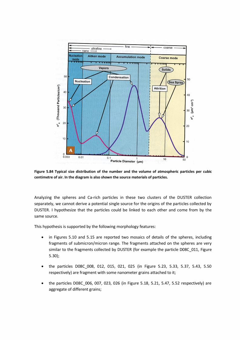
Figure 5.84 Typical size distribution of the number and the volume of atmospheric particles per cubic
centimetre of air. In the diagram is also shown the source materials of particles.
Analyzing the spheres and Ca-rich particles in these two clusters of the DUSTER collection
separately, we cannot derive a potential single source for the origins of the particles collected by
DUSTER. I hypothesize that the particles could be linked to each other and come from by the
same source.
This hypothesis is supported by the following morphology features:
in Figures 5.10 and 5.15 are reported two mosaics of details of the spheres, including
fragments of submicron/micron range. The fragments attached on the spheres are very
similar to the fragments collected by DUSTER (for example the particle D08C_011, Figure
5.30);
the particles D08C_008, 012, 015, 021, 025 (in Figure 5.23, 5.33, 5.37, 5.43, 5.50
respectively) are fragment with some nanometer grains attached to it;
the particles D08C_006, 007, 023, 026 (in Figure 5.18, 5.21, 5.47, 5.52 respectively) are
aggregate of different grains;

a particular case is the particle D08C_029 (in Figure 5.58) it looks like a small sphere
embedded in a carbon sheet. It is possible that the nanometer sphere could be a vapor
condensed particle.
All these features suggest that the particles were collected in a high dust-density environment
composed of different kind of particles and allowing the particle-particle collision and
aggregation. As an example we refer to particle D08C_029, that can be the result of a collision of
two particle of different origin.
Scenarios of an environment with high dust density could be from terrestrial, volcanic eruptions
or a very efficient power plant, or extraterrestrial sources such as a meteor fireball.
TERRESTRIAL SOURCES EXTRATERRESTRIAL SOURCES
VOLCANIC EJECTION
It is a process that products fragment and in
some cases spherules. A typical glass produced
is the Obsidian (an amorphous silicate,
transparent or opaque)
METEOROIDS
Process of heating during entry in atmosphere
with consequent ablation, evaporation and
condensation (there is no gas inside the particle
during the cooling process). Could product
fragment and spheres.
POWER PLANTS (combustion product)
In Svalbard Islands there are coal power plants.
A typical combustion product is coal fly ash
(spherules of wide size and composition)
FIREBALLS (i.e. Tagish Lake meteorite)
There is a process of ablation and
fragmentation, could produce fragment and
spheres.
Table 5.51 Hypothesis of sources from the terrestrial and from extraterrestrial environment that may
introduce dust in stratosphere.
5.5.1 Terrestrial sources
Both terrestrial sources (Table 5.51) produced dust high-density environment. Is known from
studies of El Chichòn eruption that the volcanic ash may reach 36 km of altitude and that the
particles are reach in Ca-Al-Silicate (Rietmeijer 1993). During the period of DUSTER collection
(June 2008) there were no major eruptions except for the first eruption of Chaitén (Chile)
reported on the Global Volcanism Program (Smithsonian National Museum of Natural History).
The eruption began the morning of 2 May 2008 with an ash plum of about 13.7 - 16.8 km and
reached an estimate altitude greater than 21 km. On 6 May, ONEMI (Oficina Nacional de
Emergencia - Ministerio del Interior) reported that the eruption became more forceful (Figure
5.85) and generated a wider and darker gray ash plume rising to an estimated altitude of 30 km.

Being the volcano in the south hemisphere is not probably that DUSTER collected the dust ejected
by Chaitén.
Figure 5.85 The Moderate Resolution Imaging Spectroradiometer (MODIS) on NASA's Terra satellite
captured this image of a long, cloud-like plume extending about 700 km SE from Chaitén on 3 May. The
plume rises high over the Andes mountains, drifts across Argentina, and thins over the Atlantic Ocean.
(NASA Earth Observatory and the MODIS Rapid Response System)
The other terrestrial source that allows a high dust density is the coal combustion product (CCP)
of the power plant, it produces mainly coal fly ashes. The coal is a sedimentary rock made of
organic and inorganic materials, which contain many elements. During combustion because of the
high temperature this elements are release in gaseous or solid phase. The coal fly ash spheres can
be hollow or massive.
The typical coal fly ash composition depend on burned materials, as shown on Jablonska et al.
(2001) study, about coal fly ash from Ba-enriched coal burning on Silesian Industrial Region. An
example of oxide composition is SiO2, Al2O, Fe2O3, MgO and CaO, with traces of TiO2, MnO, Na2O,
K2O, P2O5, CO2 and SO3 (Vassilev S.V. and Vassileva C.G., 1997). The traces elements are influenced
by the original composition of coal, the combustion conditions, the size and mineralogy of the
coal fly ash (Brownfield M.E. et al., 2002). For example in low temperature ashes Na2O is 14%, but
it is lost in high temperature ashes (Vassilev S.V. and Vassileva C.G., 1997).
In the Table 5.52 are reported the composition of coal fly ash of nearly pure SiO2 compared with
the composition of DUSTER spheres. In the Figure 5.86 are plotted on the ternary diagram of
Gieré et al (2003) the spheres and the fragment D08C_011 and they match with the coal fly ashes.
If the CCP of a power plant could be the source of the particles collected, the fragment attached
on the spheres could have the same nature of the fragment collected on the sample holder, and
the aggregates could be the product of the interaction between all the particles present in this
high dust density environment.

D08C_001 (#1) D08C_001 (#2) D08C_002
Coal Fly Ash
(nearly pure
SiO2)
min max
CO2 28.2 29.4
Na2O 30.3 19.7 20.6 0.02 1.16
MgO 4.1 3.1 2.9 0.05 4.03
Al2O3 0.7 0.9 0.6 1.63 60.5
SiO2 59.8 45.6 43.4 6.60 97.7
P2O5 0.11 0.63
K2O 0.05 4.13
CaO 4.3 2.5 3.1 0.06 23.1
TiO2 0.01 9.51
Cr2O3 0.01 0.06
MnO 0.01 0.03
Fe2O3 1.6 0.28 22.8
NiO <0.01 0.01
CuO 0.01 0.02
ZnO 0.02 0.06
UO2 0.01 0.04
Table 5.52 Comparison between DUSTER spheres and a typical coal fly ash nearly pure SiO2

Figure 5.86 Ternary diagrams showing the average composition of the different kinds of coal fly ash.
Symbols: large, filled square=bulk ash composition; filled circle=non-magnetic glass; filled
triangle=magnetic glass; open diamond=hematite; open circle=almandine(?); filled square=jarosite (?);
open square=Ca-rich crystalline phases. Mullite-A=Al6Si2O13, Millite-B=Al2(Al2+2xSi2-2x)O10-x (Giaré et al.
2003). The red point is the particle D08C_011, the orange point are the DUSTER spheres.
5.5.2 Extraterrestrial sources
The extraterrestrial sources described in Table 5.51 are meteoroids and fireball (or bolides) , but
only the second produced a high density dust environment.
In the DUSTER particles collection there are:
particles (Figure 5.58 and 5.63) that remind cosmic particles collected by NASA aircraft
program (Figures 5.87);
particles rich in calcium (Figure 5.79) and in particular in calcite (Table 5.44);
also the particles less than 1.5 µm are rich in oxygen and carbon and suggest carbonates
(Figure 5.78).
In Figure 5.88 there is an example of a spherical particle of cosmic origin collected by the NASA
JSC Cosmic Dust Program. In the Figure 5.89 are reported some particles collected in the lower
stratosphere by the same NASA program for the purpose of collecting stratospheric dust that
could be hypothesized to be form from the Tagish Lake dust cloud associated with this fireball
event (Cosmic Dust Catalog Vol. 17 JSC). They are shown for comparison with DUSTER particles
with respect to composition and morphology.
On 18 January 2000 at 16:43 (UT) the Tagish Lake meteoroid entered into the Earth atmosphere
with a mass of almost 2 x 10⁵ kg. It fragmented between 50 – 30 km of altitude releasing several
hundreds of fragment for a total of 1500 kg m-3. The composition of the recovered samples are an
intermediate between CM and CI meteorites (see Chapter 1) and it is consider the most primitive

solar system materials yet studied. It was surprisingly rich in carbonate minerals that vary in
composition from calcite, to siderite and magnetite (Brown et al. 2000).
Because of the similarity between DUSTER particles and the IDP collected by NASA program, an
extraterrestrial source cannot be excluded.
Figure 5.87 IDP collected by NASA IDP program (Catalogue vol.15) classified as Cosmic (?)
Figure 5.88 IDP collected by NASA IDP program (Catalogue vol.15) classified as Cosmic

Figure 5.89 Particles collected by NASA IDP program during Tagish Lake fireball. All the particles are
clssified like Cosmic. The size of the particle in the picture are: A) (28x22) µm; B) 10 µm; C) (18x13) µm.
Conclusions
In Table 5.48 are summarized the size range and the properties of stratospheric particles above
and below 30 km altitude and the particles collected by DUSTER instrument.
As discussed in the previous section, analyzing morphology and composition of particles collected
by DUSTER they fit with both sources, they could be from either terrestrial or extraterrestrial
sources.
The DUSTER particles can be divided into two different populations: the silica rich particles, and
the carbonate rich particles (Figure 5.79).
The carbonate rich population is composed of crystalline fragments and particles produced by
vapour condensation (D08C_031 and D08C_029).

This population can have extraterrestrial origin.
The silica rich population consists in: the two big spheres (D08C_001, D08C_002) and a single
fragment (D08C_011). The spheres also have attached on the surface fragments that are not
indigenous to the spheres.
The presence of fragments attached on the spheres surface suggests a possible formation in an
high dust density environment, both these two formation scenarios are plausible:
the silica rich population is produced by the same extraterrestrial event of the carbon rich
population;
the silica rich population has a terrestrial origin, formed during a volcano eruption or the
product of a power plant.
The first scenario connected to the extraterrestrial event can be excluded for silica rich population
because of the high sodium content present in the particles, in particular the spheres (see section
5.5).
Coming to the second scenario I exclude the volcano ejecta, because no volcanic events have
been registered close to the period of DUSTER collection.
Therefore I think that the most probable origin of the silica rich population is a coal combustion
environment. In this case they could have been collected on Svalbard skies as in Longyerabien
there is an active coal power plant.

6 DUSTER2009 instrument improvements and
July 2009 campaign
In this chapter the improvements of the instrument for July 2009 campaign are discussed, in
particular:
the new mechanical structure;
new configuration of sample holder, for better performances of transmission analyses;
the flight campaign and the new performances of the instrument;
a brief introduction of the preliminary particles detection and sources of contaminations.
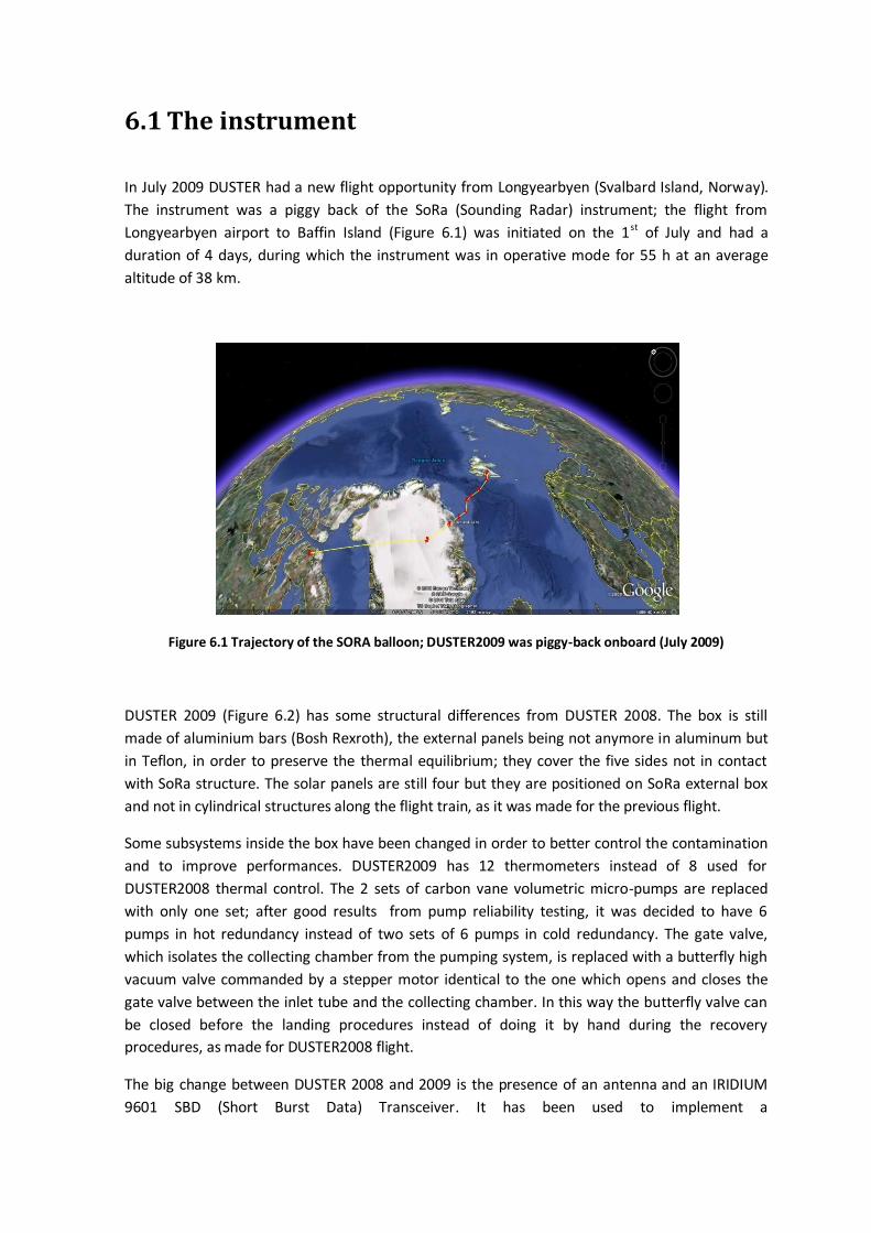
6.1 The instrument
In July 2009 DUSTER had a new flight opportunity from Longyearbyen (Svalbard Island, Norway).
The instrument was a piggy back of the SoRa (Sounding Radar) instrument; the flight from
Longyearbyen airport to Baffin Island (Figure 6.1) was initiated on the 1st of July and had a
duration of 4 days, during which the instrument was in operative mode for 55 h at an average
altitude of 38 km.
Figure 6.1 Trajectory of the SORA balloon; DUSTER2009 was piggy-back onboard (July 2009)
DUSTER 2009 (Figure 6.2) has some structural differences from DUSTER 2008. The box is still
made of aluminium bars (Bosh Rexroth), the external panels being not anymore in aluminum but
in Teflon, in order to preserve the thermal equilibrium; they cover the five sides not in contact
with SoRa structure. The solar panels are still four but they are positioned on SoRa external box
and not in cylindrical structures along the flight train, as it was made for the previous flight.
Some subsystems inside the box have been changed in order to better control the contamination
and to improve performances. DUSTER2009 has 12 thermometers instead of 8 used for
DUSTER2008 thermal control. The 2 sets of carbon vane volumetric micro-pumps are replaced
with only one set; after good results from pump reliability testing, it was decided to have 6
pumps in hot redundancy instead of two sets of 6 pumps in cold redundancy. The gate valve,
which isolates the collecting chamber from the pumping system, is replaced with a butterfly high
vacuum valve commanded by a stepper motor identical to the one which opens and closes the
gate valve between the inlet tube and the collecting chamber. In this way the butterfly valve can
be closed before the landing procedures instead of doing it by hand during the recovery
procedures, as made for DUSTER2008 flight.
The big change between DUSTER 2008 and 2009 is the presence of an antenna and an IRIDIUM
9601 SBD (Short Burst Data) Transceiver. It has been used to implement a

telecommand/telemetry (TC/TM) system allowing operations control from ground through
commanding and housekeeping data transmission. The Iridium SBD service provides: mobile
Originated (instrument) messages up to 340 bytes; low uniform global latency (less than 1
minute); mobile Terminated (experimenter) messages up to 270 bytes; global coverage. In this
way DUSTER can be perfectly independent from the gondola or the host instrument.
Figure 6.2 DUSTER 2009 instrument
6.1.1 Sample holders
In order to have an easy dismountable sample holder and to be able to perform analyses of the
collected sample in transmission mode, the sample holder used during 2009 flight has been
totally changed.
It has the same dimensions of the previous collector, but it is totally in stainless steel except for
the TEM grids that are still 300 mesh, made in gold and covered with holey carbon thin film. The
sample holder is compose of: a round base (0.5 cm thick and 2.3 cm in diameter) with a pin
allowing accommodation in the FE-SEM chamber; a thin plate (0.05 cm) pierced with 13 holes not
perfectly round, but with a little buttonhole each, to better manipulate the TEM grids; a thin plate
(0.05 cm) pierced with 13 holes that has the aim to fix the TEM grids in their positions (Figure 6.3).
Comparing this configuration with the one used on DUSTER 2008, the problem of dismount
procedure is solved, with one TEM grid less and without the FE-SEM dedicated smooth area (that
was anyhow not used in the DUSTER 2008 data analysis).

Assembling the sample holder still requires adopting all precautions foreseen in a clean room.
The sample holder assembling procedure is reported below.
Figure 6.3 DUSTER 2009 sample holder
Assembling procedure
To mount this version of the sample holder the experimenter needs a support (Figure 6.4)
designed to help in the assembling procedure and to give the right orientation to the sample
holder. In the previous type of collector we had the smooth gold surface defining an orientation
of the sample holder, while in this new type we define it with reference to the indentation of the
rim. The indentation has to be on the right and the grids are named from up to down and from
left to right as shown in Figure 6.5.
Figure 6.4 Cylinder support. In the red
circle is highlighted the reference to
orient the sample holder.
Figure 6.5 Sample holder orientation
with named grids

Before sample holder assembling, the experimenter has to be sure that all the parts are cleaned
with isopropyl alcohol and the procedure has to be done in a laminar flux bench, ensuring a clean
controlled environment.
First of all, the cylinder support has to be positioned as shown in Figure 6.4 then the base with the
pin and over it the plate with the buttonholes are inserted (Figure 6.6).
Figure 6.6 Cylinder support with the base and the plate with buttonholes
Then, the 13 TEM grids are accommodated in the holes using the micro-tweezers and helping with
the buttonhole (Figure 6.7).
Figure 6.7 Accommodation of TEM grids
The last pierced plate is positioned, being careful not to move the TEM grids and fix all with the 3
screws (Figure 6.8).

Figure 6.8 Fixing procedure of the sample holder
Helping with a screwdriver or an hex key, the sample holder is extracted from the cylinder
support (Figure 6.9). Now it is ready for SEM scanning and to be accommodate in the collecting
chamber.
Figure 6.9 Extraction procedure of the sample holder from the cylinder support
6.2 Characterization
The results of DUSTER 2008 flight are affected by two limitations: the instrument is able to collect
particles from 0.1 µm size, but the scanning resolution allowed to detect only particles larger than
0.5 µm; the second limitation is due to the gaps that sometimes occurred during scanning (see
Chapter 4).
To solve these problems the scanning procedure has been changed, adapting it to the most
probably collecting areas, and overlapping the scanning areas by 10% in order to not miss
important data. The central area with the highest probability to collect particles is represent from
the grids number 3, 4, 6, 7, 8, 10, and 11. These grids were scanned in different areas with
different resolution: an area of (20x20) meshes was scanned at 6500 magnifications, each image
corresponding to an area of (46x34) µm and a resolution of 0.045 µm each pixel. This scanning
needs 4x3h per grid, being divided into 4 areas of (10x10) meshes (Figure 6.10).

Figure 6.10 Example of TEM grid. The red squere is the area (20x20) meshes, the green squares are the
areas (10x10) meshes scanned at 6500 magnifications.
To have a better resolution of most probable collecting areas, the central grids are scanned in the
diagonal areas (5x5) meshes at 17000 magnifications (Figure 6.11) corresponding to an image
area of (17x13) µm and a resolution of 0.016 µm each pixel; each scanning needs 3h20m. The
remnants areas of the central grids were scanned at 3250 magnifications in few minutes.
Figure 6.11 Example of TEM grid, the red squares are the (5x5) meshes areas scanned at 17000
magnification.
The lateral grids (1, 2, 5, 9, 12, and 13) were scanned on the entire surface at 3250 magnifications,
corresponding to an image area of (92x69) µm and a resolution of 0.090 µm each pixel; this
scanning needs 3h50m.
The sample holder used like Blank has only four grids, three of them are scanned at 3250
magnifications and one is scanned with the same criteria of the Collector’s central grids.

6.3 Preliminary results (contamination and collected
particles identification)
The results from this campaign are still a work in progress. Only half of the grids are compared
and at a preliminary analysis we can see that DUSTER2009 surely collected particles, but at the
same time on the collector there is a lot of contamination.
This last one is composed in large amount by soot structures (Figure 6.12) due to a fire developed
after landing and involving the main payload of the flight. DUSTER was not directly involved in the
fire, but during the landing impact it loose the inlet tube (the only part protruding from the box
envelope) and this violent braking caused a leakage in the gate valve, letting some smoke enter.
Figure 6.12 Soot structure on DUSTER2009 collector.
For this reason all the soot structures will be consider contamination. They seem to be easy to
recognize, but this risks to be a lost if DUSTER2009 had collected extraterrestrial particles that has
the same morphology of soot of fire (Figure 6.13).
Figure 6.13 IDP NASA collected, Catalogue Vol.15 Johnson Space Centre

The new particles recognized until now, looking at the morphology could be aggregates of
condensed particles or dust embedded with soot contamination (Figure 6.14); only compositional
analyses will define the origins of these particles. Up to now we haven’t identify particles of the
size and shape of the two spheres collected during DUSTER 2008 campaign, this would be a proof
that particles larger than 100 µm size (too big for DUSTER flow rate) were fortuitous collected.
Figure 6.14 Collected particle on DUSTER2009 collector, it could be a fragment embedded with soot
structures or an aggregate of condensed.
Conclusions
DUSTER2009 is really autonomous with respect to the 2008 instrument tanks to the own
telemetry, and it is designed to better preserve the samples from contamination thanks to the
second stepper motor that seal the collecting chamber before the landing procedure. The sample
holder is perfectly dismountable and do not damage the TEM grids. From the structural point of
view the instrument is improved and it is made autonomous.
For what concern the capability to collect particles, this version of the instrument is more
performing than the previous one, but this need to be confirmed based on evaluation of collected
particles. Future FESEM-EDX analyses will tell us what kinds of particles have been collected and
their size distribution.

Conclusions and future developments
DUSTER is an instrument able to collect dust in the upper stratosphere (30 – 40 km). In the last
three years it performed two flights successfully completed. My work was mainly focused on the
study of the sample holder structure, in order to facilitate the analyses, preserve the
contamination control, and to respect the scientific requirements, and on the analysis of the
collected particles. The results concern mainly the DUSTER2008 campaign.
The particles recognized as collected during the DUSTER2008 campaign are 25 in the size range
(0.5 – 7.0) µm and two spheres of more than 100 µm . The size range has a main bias in the
inferior limit due to the limitation in scanning automatic procedures that not allow to detect
particle less than 0.5 µm. Another bias source is due to the holey carbon film substrate, if a
particle goes through the holes of the carbon film it is not possible to detect it.
The analyses (FESEM-EDX, FT-IR and Raman) shown silica-rich and calcium carbonates particles.
The morphological study suggests that the particles were collected in a dust high density
environment probably created by a single source.
Two different scenarios are possible:
1. a terrestrial sources, for example a volcanic ejection or an efficient power plant;
2. an extraterrestrial event that create a lot of fragment, such as a fireball as Tagish Lake
(18th January 2000).
The analyses cannot exclude one of the two sources, the only things sure is that in the period of
DUSTER collection there were not volcanic ejection except for Chaitén (Chile) in May 2008, but it
is in the Southern hemisphere and is improbable that its volcanic ashes reached the Northern
stratosphere.
The possibility of the two alternative explanations (terrestrial or extraterrestrial origin) highlight
the importance to study the composition of the stratospheric dust above 30 km. The study of the
extraterrestrial dust component could provide information on the Solar System origins. The
terrestrial component gives information on the terrestrial (natural or anthropogenic)
contamination of the stratosphere.
The upper stratosphere is a boundary atmospheric layer where terrestrial and extraterrestrial
components coexist, and both have to be studied as determinant factors for climate changing, in
local and global scale.
DUSTER2009 was the second successful campaign performed during the last three years. We have
not yet final results, the collected particle identification work is in progress. This flight opportunity
was the occasion to test the new sample holders configuration. They had a good behavior and
preserve the integrity of the TEM grids, by laboratory tests it is proved that they are easily
dismountable to allow transmission analyses. A future work for sample holders structure is to find
a material to have a smooth surface in order to have a collection surface dedicated to the FESEM
analysis.

Another open point for future works is to elaborate a procedure for automatic comparison of the
images taken by FESEM to characterize the sample holders pre and post flight, to shorten the
collected particles identification phase.
Next DUSTER flight opportunity will be next February (2011) from Kiruna (Sweden), with the
CNES (Centre National d'Études Spatiales) support. DUSTER will fly again in a piggy-back
configuration demonstrating that the instrument is sufficiently small and light to be guest by a
spread variety of balloon campaign.
The final aim of this project is that DUSTER could become a long-term program for high
stratospheric dust collection, of terrestrial and extraterrestrial origin. The results of this collection
program would be of critical interest for a wide interdisciplinary community.

Bibliography
Anders E., & Grevesse N.,1989.Abundance of the elements: Meteoritic and Solar. Geochem and
Cosmochem Acta Vol. 53 Issue 1 pp. 197-214.
Angell J.K., 1997. Stratospheric worming due to Agung, El Chichon, and Piatubo taking into
account quasi-biennial oscillation. J Geophys Res Vol.102.
Berthet G., Renard J.B., Brogniez C., Robert C., Chartier M., Pirre M., 2002. Optical and physical
properties of stratospheric aerosols from balloon measurements in the visible and near-infrared
domains. I. Analysis of aerosol extinction spectra from the AMON and SALOMON balloonborne
spectrometers. Applied Optics, Vol.41.
Biermann U.M., Presper T., Koop T., Möinger J., Crut-zen P.J., Peter T., 1996. The unsuitability of
meteoritic and other nuclei for polar stratospheric cloud freezing. Geophysical Research Letters.
Vol. 23, pp. 1693 – 1696.Brownfield M.E., Affolter R.H., Cathcart J.D., Meeker G.P., Rice C.A.,
Zielinski R.A., Hower J.C., 2002. Characterization and Models of Occurrence of Elements in Feed
Coal and Fly Ash - An integrated approach. USGS Fact Sheet-038-02 May.
Bigg E.K., Ono A., Thompson W.J., 1970. Aerosols at altitudes 20 and 37 km. Tellus XXII, 5, pp.550-
563.
Bigg E.K., Kviz Z., Thompson W.J., 1971. Electron microscope photographs of extraterrestrial
particles. Tellus XXIII, 3, pp.247-260.
Brenninkmeijer C.A.M., Zahn A., Maiss M., Crutzen P.J., Cuijpers H., Van Velthoven P.F.J., 1998.
The 13C, 14C, and 18O isotope composition of CO at 10 km between the tropics and the mid-
latitudes; results from the CARIBIC project. American Geophysical Union (AGU), fall meeting, San
Francicso, 6-10 December.
Brown P.G, Hildebrand A.R., Zolensky M.E., Grady M., Clayton R.N., Mayeda T.K., Tagliaferri E.,
Spalding R., MacRae N.D., Hoffman E.L., Mittlefehldt D.W., Wacker J.F., Bird J.A., Campbell M.D.,
Carpenter R., Gingerich H., Glatiotis M., Greiner E., Mazur M.J., McCausland P.JA., Plotkin H.,
Mazur T.R., 2000. The Fall, Recovery, Orbit, and Composition of the Tagish Lake Meteorite: A New
Type of Carbonaceous Chondrite. Science Vol.290, pp. 320-325.
Brownlee D.E., Hodge P.W., 1973. Ablation debris and primary micrometeoroids in stratosphere.
Space Res Vol.13.
Brownlee D.E., Ferry G.V., Tomandl D., 1976. Stratospheric aluminium oxide. Science Vol.191.
Chandra S., 1993. Changes in stratospheric ozone and temperatures due to the eruptions of Mt.
Pinatubo. Geophys Res Lett Vol.20.
Curtius J., Weigel R., Vossing H.J., Wernli H., Werner A., Volk C.M., Konopka P., Krebsbach M.,
Schiller C., Roiger A., Schlager H., Dreiling V., Borrmann S., 2005. Observations of meteoritic

material and implications for aerosol nucleation in the winter Arctic lower stratosphere derived
from in situ particle measurements. Amos Chem Phys Discuss Vol.5.
Cziczo D.J., Thomson D.S., Murphy D.M., 2001. Ablation, Flux, and Atmospheric Implications of
Meteors Inferred from Stratospheric Aerosol. Science Vol.291.
Dahl K. and Buchardt B., 2006. Monohydrocalcite in the arctic Ikka Fjord, SW Greenland: First
reported marine occurrence. Joural of Sedimentary Research, Vol. 76, 460-471.
Della Corte V., Palumbo P., De Angelis S., Ciucci A., Brunetto R., Rotundi A., Rietmeijer F.J.M., Zona
E., Bussoletti E., Colangeli L., Esposito F., Mazzotta Epifani E., Mennella V., Peterzen S., Masi S.,
Ibba R., (2010). DUSTER (Dust in the Upper Stratosphere Tracking Experiment and Retrieval): a
balloon-borne dust particle collector. (in press)
Deshler, T., Hervig, M.E., Hofmann, D.J., Rosen, J.M., Liley, J.B., 2003. Thirty years of in situ
stratospheric aerosol size distribution measurements from Laramie, Wyoming (41°N), using
balloon-borne instruments. Journal of Geophysical Research 108 (D5.), 4167.
Deshler, T., 2008. A review of global stratospheric aerosol: Measurements, importance, life cycle,
and local stratospheric aerosol. Atmospheric Research 90, 223–232.
Di Sarra A., Cacciani M., Fiocco G., Fuà D., Jørgensen T.S., 2002. Lidar observations of polar
stratospheric clouds over northern Greenland in the period 1990–1997. Journal of Geophysical
Research Vol.107, No. D12, pp. 4152-4167.
Dutton E.G., Christy J.R., 1992.Solar radiative forcing at selected locations and evidence for global
lower tropospheric cooling following the eruption of El Chichon and Pinatubo. Geophys Res Lett
Vol.19.
Flynn G.J., 1997. Collecting interstellar dust grains. Nature, Vol.387.
Genge M.J., Engrand C., Gounelle M., Taylor S. 2008. The classification of micrometeorites.
Meteoritics & Planetary science Vol. 43, No 3, 497 – 515.
Gieré R., Carleton L.E., Lumpkin G.R., 2003. Micro- and nanochemistry of fly ash from coal-fired
power plant. American Mineralogist, Vol. 88, pp.1853 – 1865.
Grün E., Zook H.A., Fechtig H., Giese R.H., 1985. Collisional balance of the meteoritic complex.
Icarus, Vol. 62, No 244.
Grün E., Gustafson B., Mann I., Baguhl M., Morfill G.E., Staubach P., Taylor A., Zook H.A., 1994.
Interstellar dust in the heliosphere. Astronomy and Astrophysics, Vol. 286, pp. 915-924.
Hanson D.R., Lovejoy E.R., 1995. The reaction of ClONO2 with submicrometer sulfuric acid
aerosol. Science 267, 1326–1328.
Hofmann D.J., Rosen J.M., Harder J.W., Hereford J.V., 1989. Balloon-borne measurements of
aerosol condensation nuclei, and cloud particles in the stratosphere at McMurdo Station,
Antarctica, during the spring of 1987. J Geophys Res Vol.94.

Hofmann D.J., 1990. Measurement of the condensation nuclei profile to 31 km in the Arctic in
January 1989 and comparison with Antarctic measurements. Geophys Res Lett Vol.17.
Hofmann D.J., Oltmans S.J., Harris J.M., Komhyr W.D., Lathrop J.A., Defoor T., Kuniyuki D., 1993.
Ozone sonde measurements at Hilo, Hawaii following the eruption of Pinatubo. Geophys Res Lett
Vol.20.
Hunten D.M., Turco R.P., Toon O.B., 1980. Smoke and dust particles of meteoritic origin in the
Mesosphere and Stratosphere. J Amos Sci Vol.37.
Junge C.E., Chagon C.W., Manson J.E., 1961. Stratospheric Aerosols. Journal of Meteorology
Vol.18.
Kent G.S., Farrukh U.O., Wang P.H., Deepak A., 1988. SAGE I and SAM II measurements of 1 µm
Aerosol Extinction in the free Troposphere. Journal of applied meteorology, Vol.27.
Kerr R.A., 1983. El Chichon climate effect estimated. Science 219.
Landgraf M., Baggaley W.J., Grun E., Kruger H., Linkert G., 2000. Aspects of the mass distribution
of interstellar dust grains in the solar system from in sit measurements. Journal of Geophysical
Research, Vol.105, No. A5, pp10343-10352.
Love S.G. and Brownlee D.E., 1994. Peak atmospheric entry temperatures of micrometeorites.
Meteoritics 29, pp. 67-70.
Luo K., Xu L., Li R., Xiang L., 2002. Fluoine emission from combustion of steam coal of North China
Plate and Northwest China. Chinese Science Bulletin, Vol. 47, No. 16, pp. 1346 – 1350.
Martinsson B.G., Nguyen H.N., Brenninkmeijer C.A.M., Zahn A., Heintzenberg J., Hermann M., van
Velthoven P.F.J., 2005. Characteristics and origin of lowermost stratospheric aerosol at northern
midlatitudes under volcanically quiescent conditions based on CARIBIC observations. Journal of
Geophysical Research, Vol.110, No. D12201.
Mateshvili N. and Rietmeijer F.J.M., 2002. Stratospheric dust loading from early 1981 to
September 1985 based on the twilight sounding method and stratospheric dust collections. J
Volcanol Geother Res Vol 120.
Mateshvili N., Fussen D., Vanhellemont F., Bingen C., Kyrola E., Mateshvili I., Mateshvili G., 2005.
Twilight sky brightness measurements as a useful tool for stratospheric aerosol investigations. J
Geophys Res Vol.110.
McDonnell J.A.M., Berg O.E., 1975. Space Research Vol. 15, No. 555.
Meckinnon I.D.R, McKay D.S., Nace G., Isaacs A.M., 1982. Classification of the Johnson Space
Center Dust Collection. Proceedings of the thirteenth lunar and planetary science conference ,
part1 Journal of geophysical research, vol.87, supplement, pages A413-A421, November 15.
McCormick M.P., Hamill P., Pepin T.J., Chu V.P., Swissler T.J., McMaster L.R., 1979. Satellites
studies of the stratospheric aerosol. Bull Amer Meteor Soc vol.60.

McCormick, M.P., Thomason, L.W., Trepte, C.R., 1995. Atmospheric effects of the Mt. Pinatubo
eruption. Nature 373, 399.
Murphy D.M., Thomson D.S., Mahoney M.J., 1998. In Situ Measurements of Organics, Meteoritic
Material, Mercury, and Other Elements in Aerosols at 5 to 19 Kilometers. Science Vol.282.
Parker D.E., Brownscombe J.L., 1983. Stratospheric worming following the El Chichon volcanic
eruption. Nature Vol.301.
Pitari G., 1993. A numerical study of the possible perturbation of stratospheric dynamics due to
Pinatubo aerosols – Implication for tracer transport. J Atmos Sci Vol.50.
Plane J.M.C., 2003. Atmospheric Chemistry of Meteoric Metals. Chem. Rev. Vol. 103, pp. 4963-
4984.
Pueschel R. F, Kinne S.A., 1995. Physical and radiative properties of Arctic atmospheric aerosols.
The Science of the Total Environment, Vol. 160, pp. 811 – 824.
Qing Sun, Guoqiang Chu, Jiaqi Liu, Denyi Gao, 2006. A 150 – year Record of Heavy Metals in the
Varved Sediments of Lake Bolterskardet, Svalbard. Arctic, Antarctic, and Alpine Research, Vol. 38,
No. 3, pp. 436 – 445.
Renard J.-B., Ovarlez J., Berthet G., Fussen D., Vanhellemont F., Brogniez C., Hadamcik E., Chartier
M., Ovarlez H. 2005. Optical and physical properties of stratospheric aerosols from balloon
measurements in the visible and near-infrared domains. III. Presence of aerosols in the middle
stratosphere. Applied Optics, Vol.44, No.19, pp. 4086 – 4095.
Rietmeijer F.J.M., 1989. Tin in a chondritic interplanetary dust particle. Meteoritical society 24, 43
- 47.
Rietmeijer F.J.M. (1993) Volcanic dust in the stratosphere between 34 and 36 km altitude during
May, 1985. J. Volc. Geothermal Res. 55, 69-83.
Rietmeijer F.J.M., 2000. Interrelationships among meteoric metals, meteors, interplanetary dust,
micrometeorites, and meteorites. Meteoritics Planet Science, Vol. 35, pp. 1025 – 1041.
Rietmeijer F.J.M., 2002. The Earliest Chemical Dust Evolution in the Solar Nebula. Chemie der
Erde, Geochemistry, 62, 1, pp. 1-88.
Rodhe H., 1985. The transport of sulphur and nitrogen through the remote atmosphere. The
Biochemical Cycling of Sulphur and Nitrogen in the Remote Atmosphere, Galloway J.N. et al., Eds.,
NATO ASI Series C, Vol. 159, 105 – 124.
Rotundi A., Rietmeijer F.J.M., Brucato J.R., Colangeli L., Mennella V., Palumbo P., Bussoletti E.,
2000. Refractory comet dust analogues by laser bombardment and arcdischarge production: a
reference frame for ``dusty experiments'' on-board ROSETTA. Planetary and Space Science, Vol.
48, pp.371-384.

Saxena V.K., Shaocai Yu, Anderson J., 1997. Impact of stratospheric volcanic aerosols on climate:
evidence for aerosol shortwave and longwave forcing in the southeastern U.S. Atmospheric
Environment, Vol. 31, No. 24, pp. 4211-4221.
Taylor S., Lever J.H., Harvey R.P., 2000. Numbers, types and compositions of an unbiased
collection of cosmic spherules. Meteoritics & Planetary science 35, 651 – 666.
Testa Jr.J.P., Stephens J.R., Berg W.W., Cahill T.A., Onaka T., 1990. Collection of microparticles at
high balloon altitudes in the stratosphere. Earth and Planetary Science Letters, Vol.98.
US Standard Atmosphere 1976. U.S. Government Printing Office, Washington, D.C., 1976
Vassilev S.V. and Vassileva C.G., 1997. Geochemistry of coals, coal ashes and combustion wastes
from coal-fired power stations. Fuel processing technology 51, 19-45.
Wilson J.C., Stolzenburg M.R., Clark W.E., Loewenstein M., Ferry G.V., Chan K.R., 1990.
Measurement of condensation nuclei in the airborne Arctic stratospheric expedition:
Observations of particle production in the polar vortex. Geophys Res Lett, Vol.17.
Wilson J.C., Stolzenburg M.R., Clark W.E., Loewenstein M., Ferry G.V., Chan K.R., Kelly K.K. 1992.
Stratospheric sulfate aerosol in and near the Northern Hemisphere polar vortex: The morphology
of the sulfate layer, multimodal size distributions, and the effect of denitrification. J Geophys Res
Vol.97.
Xu, L., Okada, K., Iwasaka, Y., Hara, K., Okuhara, Y., Tsutsumi, Y., Shi, G., 2001. The composition of
individual aerosol particle in the troposphere and stratosphere over Xianghe (39.45°N, 117.0°E),
China. Atmospheric Environment, 35.
Zolensky M.E. and Mackinnon I.D.R., 1985. Accurate stratospheric particles size distribution for a
flat plate collection surface. J Geophys Res.
Zolensky M.E., McKay D.S., Kaczor L.A., 1989. A tenfold increase in the abundance of large solid
particles in the stratosphere, as measured over the period 1976-1984. J Geophys Res Vol.94.
Zolensky M.E. and Warren J.L., 1994. Collection and curation of interplanetary dust particles
recovered from the stratosphere. Conf Proc Workshop on Analysis of IDPs.

Acknowledgements
I wish to thank Prof. Pasquale Palumbo, Prof. Alessandra Rotundi and Ing. Della Corte Vincenzo,
for the support they gave me with theirs advices and to be a guide during these last three years.
I wish to sincerely express my gratitude to Prof. Frans J.M. Rietmeijer to be a lighthouse in the
darkness.
A special thank to all my family that support me in every step of my life.
A particular thanks goes to the marvelous friends, to be near me in each good and bad moment,
thanks to Mauro, Michele, Simone and Vincenzo.
Thanks also to all the group of ‘Laboratorio di Fisica Cosmica e Planetologia’ and to Antonella
Continanza.
Last but not least thanks to Prof. Antonio Moccia for his valuable availability as coordinator of the
Aerospace Engineer PhD school.
I apologize if I forgot someone.