Finance and Economics Discussion SeriesDivisions of Research & Statistics and Monetary Affairs
Federal Reserve Board, Washington, D.C.
Strategic Liquidity Mismatch and Financial Sector Stability
Andre F. Silva
2019-082
Please cite this paper as:Silva, Andre F. (2019). “Strategic Liquidity Mismatch and Financial Sector Stability,”Finance and Economics Discussion Series 2019-082. Washington: Board of Governors of theFederal Reserve System, https://doi.org/10.17016/FEDS.2019.082.
NOTE: Staff working papers in the Finance and Economics Discussion Series (FEDS) are preliminarymaterials circulated to stimulate discussion and critical comment. The analysis and conclusions set forthare those of the authors and do not indicate concurrence by other members of the research staff or theBoard of Governors. References in publications to the Finance and Economics Discussion Series (other thanacknowledgement) should be cleared with the author(s) to protect the tentative character of these papers.
Strategic Liquidity Mismatchand Financial Sector Stability
Andre F. Silva
Federal Reserve Board
April 23, 2019
Review of Financial Studies, forthcoming
Abstract
This paper examines whether banks strategically incorporate their competitors’ liquiditymismatch policies when determining their own and the impact of these collective decisionson financial stability. Using a novel identification strategy exploiting the presence ofpartially overlapping peer groups, I show that banks’ liquidity transformation activityis driven by that of their peers. These correlated decisions are concentrated on theasset side of riskier banks and are asymmetric, with mimicking occurring only whencompetitors take more risk. Accordingly, this strategic behavior increases banks’ defaultrisk and overall systemic risk, highlighting the importance of regulating liquidity risk froma macroprudential perspective. (JEL G01, G20, G21, G28)
*I thank the editor, Philip Strahan, and two anonymous referees for their extremely helpful comments. Iam also grateful to Thorsten Beck, Pawel Bilinski, and Paolo Volpin for their guidance and encouragement.For valuable comments and suggestions, I thank Sofia Amaral, Jennie Bai, Tobias Berg, Lamont Black(discussant), Max Bruche, Barbara Casu, Ricardo Correa, Olivier de Bandt (discussant), Hans Degryse,Thomas Eisenbach (discussant), Miguel Ferreira, Michael Gofman (discussant), Michael Koetter, MartienLamers (discussant), Andreas Lehnert (discussant), Helge Littke (discussant), Camelia Minoiu, Steven Ongena,Jose-Luis Peydro, Andrea Presbitero, Joao Santos, Glenn Schepens, Enrique Schroth, Jason Sturgess, WolfWagner, Ansgar Walther, and seminar and conference participants at the Federal Reserve Board, University ofOxford, Universitat Pompeu Fabra, Nova SBE, INSEAD, Rotterdam School of Management, Warwick BusinessSchool, Queen Mary University of London, KU Leuven, Bank of England, European Central Bank, CassBusiness School, NYU/UoF 8th International Risk Management Conference, 1st IWH/FIN/FIRE Workshopon Challenges to Financial Stability, University of Cambridge/FNA Financial Risk and Networks Conference,Bank of Finland/ESRB/RiskLab Conference, Banco de Mexico/CEMLA/University of Zurich Conference, 4thEBA Policy Research Workshop, Federal Reserve Bank of Cleveland/OFR 2015 Financial Stability Conference,21st Spring Meeting of Young Economists, 2017 AEA Annual Meeting, 5th MoFiR Workshop on Banking, andCEPR/Bank of Israel Systemic Risk and Macroprudential Policy Conference. This paper is part of my Ph.D.thesis at Cass Business School, City, University of London. Part of this research was completed while I wasvisiting Columbia Business School, whose hospitality is greatly acknowledged. The views expressed in thispaper should not be attributed to the Board of Governors of the Federal Reserve System or other members ofits staff. Send correspondence to Andre F. Silva, 20th Street and Constitution Avenue NW, Washington, DC20551; Telephone: (202) 973-5071. Email: [email protected].
1
1 Introduction
Banks have a unique ability to create liquidity by financing illiquid, long-maturity assets such
as corporate loans with liquid, short-term liabilities such as demand deposits (Diamond and
Dybvig, 1983). This combination of lending and deposit-taking activities protects firms and
households against idiosyncratic and systematic liquidity shocks (Kashyap, Rajan, and Stein,
2002; Gatev and Strahan, 2006) and promotes economic growth (Bencivenga and Smith, 1991;
Berger and Sedunov, 2017). However, due to their fundamental liquidity provision role, banks
are also intrinsically fragile. As exposed by the 2007–2009 financial crisis, excessive liquidity
mismatch can lead to bank runs, the breakdown of wholesale markets, and distressed asset
sales that threaten the solvency of individual banks and the financial system (Brunnermeier,
2009; Tirole, 2011). Nonetheless, as recent theoretical literature emphasizes, the relationship
between excessive liquidity transformation and financial instability can be exacerbated even
further when banks engage in strategic risk-taking behavior in the form of common portfolio
choices (e.g., Farhi and Tirole, 2012; Albuquerque, Cabral, and Guedes, 2019).1 Using a novel
identification strategy exploiting the presence of partially overlapping peer groups, this paper
shows empirically that banks do take correlated portfolio decisions and that such strategic
behavior has a negative impact on the stability of the financial sector.
The incentive for banks to engage in collective risk-taking strategies can be rationalized
on different grounds. Ratnovski (2009), Farhi and Tirole (2012), and Acharya, Mehran, and
Thakor (2016), among others, suggest that this behavior occurs due to the presence of bailout
guarantees in case of generalized distress. This “too many to fail” problem (Acharya and
Yorulmazer, 2007, 2008; Brown and Dinc, 2011) leads to time-inconsistent and imperfectly
targeted support to distressed banks to prevent contagion and makes their balance sheet choices
strategic complements. Correlated portfolio choices can also be driven by contractual features
in the compensation of bank managers. In fact, Albuquerque, Cabral, and Guedes (2019)
1While in the subprime mortgage crisis the commonality of asset portfolios at banks was in the form ofreal estate loans, correlated portfolio choices during booms have been observed in various other forms in manycrises throughout history (Reinhart and Rogoff, 2009).
2
show that relying on relative performance evaluation (RPE) in compensation packages leads
managers to disproportionately choose investments that are correlated with with those of their
peers. While public guarantees would magnify this mechanism, RPE and associated correlated
portfolio choices generate systemic risk even in the absence of a lender of last resort (LOLR).2
Ultimately, commonality in portfolio exposures and unreasonably high liquidity transformation
activity may have a considerably negative impact on financial stability due to higher correlation
of defaults, inefficient contagious liquidations, and amplification of the impact of liquidity
shocks (Allen, Babus, and Carletti, 2012; Acharya and Naqvi, 2012; Acharya and Thakor,
2016). This can sow the seeds for crises associated with costly recessions and significant
distributional consequences (Reinhart and Rogoff, 2009).3
While theoretically intuitive, identifying peer effects is empirically challenging since strategic
reactions are intrinsically simultaneous (i.e., the reflection problem) and due to potential
correlated effects in which all banks in the same local network are subject to unobserved
shocks that lead them to choose similar policies (Manski, 1993). To counter these issues, I
use an identification strategy based on Bramoulle, Djebbari, and Fortin (2009) and De Giorgi,
Pellizzari, and Redaelli (2010) in which a structure of connections resembling a social network
can be used to solve the reflection problem and construct a valid instrumental variable to
account for potential correlated effects. The key feature I exploit is that large cross-border
bank holding companies tend to manage liquidity on a global scale and coordinate their
risk-management policies within the group (e.g., Cetorelli and Goldberg, 2012a,b; Anginer,
Cerutti, and Martinez Peria, 2017). Thus, while not part of the direct peer group of a
domestic bank i for liquidity mismatch decision-making, a foreign bank holding group should2Similarly, Ozdenoren and Yuan (2017) predict that when agents have incentives to match industry average
efforts, contractual externalities from RPE generate excessive systemic risk-taking. Phelan (2017) and Morrisonand Walther (2019) also show that correlated exposures may not necessarily be driven by distorted incentivesdue to bailout guarantees but as a mechanism to provide ex-post incentives for enforcement and create marketdiscipline. Common portfolio choices may also arise due to learning (i.e., free-riding in information acquisition)that can lead to inefficient outcomes with fully rational agents (Banerjee, 1992). In such case, banks may putmore weight on the choices of others than on their own information, particularly when others are perceived ashaving greater expertise (Bikhchandani, Hirshleifer, and Welch, 1998).
3Analyzing 17 advanced economies from 1870 to 2013, Jorda, Richter, Schularick, and Taylor (2017) findthat credit growth on the asset side of banks’ balance sheet and liquidity mismatch indicators are betterpredictors of systemic financial crises than solvency measures such as capital ratios.
3
still indirectly influence the policies of the domestic bank i if such holding company has a
subsidiary a that operates in the same country as bank i and that is part of i’s local network.
This structure of informal decision networks, in line with the theoretical literature on the
potential drivers of banks’ collective risk-taking strategies, generates “peers of peers” that
act as exclusion restrictions to solve the reflection problem. In addition, the policies of such
indirect peers can be used as a valid instrument that is orthogonal to the liquidity policies of
the domestic banks’ peers.
Using a sample of 1,584 commercial banks operating in OECD countries from 1999 to 2014
and the Berger and Bouwman (2009) liquidity creation measure to capture banks’ liquidity
transformation activity, I first show that financial intermediaries follow the liquidity mismatch
policies of their competitors when determining their own. The estimates indicate the economic
impact is large and consistent with coordinated behavior where banks constantly adjust to
one another’s decisions. Specifically, a one-standard-deviation increase in peer banks’ average
liquidity creation leads to a 5–9 percentage point increase in the liquidity created by individual
banks, corresponding to a 16–28% increase relative to the mean. Importantly, these findings
are robust to a battery of tests, including numerous peer group definitions, the inclusion of
country-year fixed effects to address any remaining omitted variable concerns, an alternative
instrument based on market data following Leary and Roberts (2014), as well as the use of the
Bai, Krishnamurthy, and Weymuller (2018) Liquidity Mismatch Index (LMI) and the Basel
III Net Stable Funding Ratio (BCBS, 2014) as alternative, though complementary, liquidity
mismatch indicators.
Given the importance of liquidity created off the balance sheet through loan commitments,
standby letters of credit, and other claims to liquid funds (e.g., Kashyap, Rajan, and Stein,
2002), I also consider a more granular quarterly sample of 472 commercial banks operating in
the United States during the same period. The estimated coefficients remain economically and
statistically significant, as well as remarkably similar in terms of magnitude across the liquidity
creation measures with and without off–balance sheet exposures. This confirms the results are
4

robust to the use of higher frequency data and shows that competitors have a negligible impact
in the liquidity created by banks off the balance sheet. In fact, when decomposing aggregate
liquidity creation into its individual components, I find that the peer effects are concentrated
in the asset side of liquidity creation, of which lending is a key element. This result, present in
both samples, supports previous evidence pointing toward herding behavior in banks’ lending
policies (Rajan, 1994; Uchida and Nakagawa, 2007).
In terms of cross-sectional heterogeneity, I show that peer effects in liquidity mismatch
decisions are concentrated in ex ante riskier banks with lower profit stability, distance to
default, and capital ratios, with the latter suggesting that higher levels of funding liquidity risk
are not being compensated with higher capital ratios that could increase a bank’s probability
of survival during crises (Berger and Bouwman, 2013). I also find that large and small banks’
liquidity mismatch decisions are only sensitive to the choices of their respective counterparts—a
result indicating that learning (i.e., free-riding in information acquisition) is unlikely to play a
major role in this setting. Additionally, such mimicking behavior is relatively stronger among
larger banks. This finding is not only consistent with large banks taking more risk than small
banks in equilibrium since they internalize that their decisions directly affect the government’s
optimal bailout policy (Davila and Walther, 2018), but also with risk-taking being driven by
the presence of RPE in compensation schemes that tends to be more prevalent among larger
banks (Albuquerque, Cabral, and Guedes, 2019).
Finally, I find that strategic complementarity in liquidity mismatch policies significantly
affects the stability of the financial sector. To examine the direction in which these peer effects
operate, I first show that the response of individual banks to the choices of competitors is
asymmetric. Specifically, individual banks mimic their respective peers only when competitors
are increasing funding liquidity risk, thus suggesting that banks’ behavior is indeed strategic.
I then show explicitly that, consistent with theoretical predictions (e.g., Allen, Babus, and
Carletti, 2012), correlated liquidity transformation activities increase both individual banks’
5
default risk and overall systemic risk. Together, these results emphasize the importance of
regulating liquidity risk from a macroprudential perspective.
This paper contributes to the literature by empirically showing that banks engage in
strategic and correlated portfolio decisions that threaten the stability of the financial sector.
Despite extensive research on this issue (e.g., Ratnovski, 2009; Farhi and Tirole, 2012; Vives,
2014; Ozdenoren and Yuan, 2017; Albuquerque, Cabral, and Guedes, 2019), most conclusions
are based on theoretical results that lack empirical support. In fact, while there is some
evidence of peer effects in banks’ lending policies (Uchida and Nakagawa, 2007) and liquidity
risk-management decisions (Bonfim and Kim, 2019), these studies are not able to disentangle
whether this behavior is driven by banks simply facing common unobserved shocks or sharing
common characteristics that lead them to choose similar policies. In addition, this is to the
best of my knowledge the first study empirically examining the impact of banks’ collective
liquidity mismatch decisions on financial sector stability. This issue is particularly relevant
after the 2007–2009 global financial crisis, with both academics and policymakers questioning
the efficacy of recent liquidity regulatory reforms (e.g., Calomiris, Heider, and Hoerova, 2015;
Diamond and Kashyap, 2016; Segura and Suarez, 2017).4
While broadly consistent with the literature on bailout guarantees and individual banks’
risk-shifting behavior (e.g., Dam and Koetter, 2012), the results also show that moral hazard
is not necessarily confined to banks exogenously engaging in excessive risk-taking. Instead,
banks can also create aggregate risk by mimicking one another’s balance sheet structures and
behaving strategically. Besides, unlike Gropp, Hakenes, and Schnabel (2011), the identification
framework I use does not restrict collective risk-taking behavior to be driven by distorted
incentives due to the presence of the LOLR. Instead, consistent with the theoretical predictions
4As distinctly argued by Allen and Gale (2017), “with capital regulation there is a huge literature butlittle agreement on the optimal level of requirements. With liquidity regulation, we do not even know whatto argue about.” Ultimately, the Basel III liquidity requirements may play only a limited role in reducing thelikelihood of a system-wide liquidity strain, as these requirements target individual banks and abstract fromthe additional risk of simultaneous liquidity shortfalls due to interconnections between them (IMF, 2011).
6
of Albuquerque, Cabral, and Guedes (2019), the results suggest that contractual features in
bank managers’ compensation schemes can also play an important role.5
2 Identification Strategy
Empirical Model. Let a given bank i operating in country j at time t be part of a peer group
Ni,j,t containing a total of ni,j,t peers. Let yi,j,t be the liquidity mismatch position of bank i,
and Xi,j,t and Zj,t a set of observed bank and country characteristics, respectively. Following
the standard linear-in-means model of Manski (1993), bank i’s outcome yi,j,t can be expressed
as a function of (i) the mean outcome of its peer group y−i,j,t, (ii) average characteristics of its
peer group X−i,j,t−1, and (iii) bank i’s and country j’s characteristics:
yi,j,t = µi + βy−i,j,t + λ′X−i,j,t−1 + γ′Xi,j,t−1 + δ′Zj,t−1 + vt + εi,j,t (1)
where,
y−i,j,t =∑
c∈Ni,j,t yc,j,t
ni,j,t
; X−i,j,t =∑
c∈Ni,j,t Xc,j,t
ni,j,t
The coefficient β captures the endogenous effect this paper aims to document—the influence
of peers’ liquidity mismatch choices on the respective decisions of bank i. Since bank i is
excluded, y−i,j,t varies not only across countries and over time, but also across banks within each
country-year combination. The contextual effects in X−i,j,t−1 capture the propensity of bank i
to change its liquidity transformation policy in response to changes in other characteristics of
the peer group such as capital or profitability (e.g., Blume, Brock, Durlauf, and Jayaraman,
2015). Peer-, bank-, and country-level controls are lagged by one period to mitigate concerns
of reverse causality. Bank and time fixed effects are represented by µi and vt, respectively.
5This paper also complements the recent and growing literature showing that competitors have a significantrole on individual firms’ decision-making. Empirical evidence on peer effects in corporate actions shows thatcompetitors affect firms’ capital structure choices (Leary and Roberts, 2014), stock splits (Kaustia and Rantala,2015), and dividend payment decisions (Grennan, 2019). Survey evidence also indicates that a significantnumber of CFOs consider the financing decisions of the competitors important when determining their own(Graham and Harvey, 2001).
7
Identification Problem. Identifying peer effects is notoriously difficult because of two
well-known issues: (i) the reflection problem, a particular case of simultaneity, and (ii) potential
correlated or common group effects (Manski, 1993).
First, in standard linear-in-means models in which peer groups are fixed, reflection arises
because all agents in a given local network Nijt affect and are affected by all other agents. As a
result, one cannot disentangle if bank i’s decision is the cause or the effect of its peers’ respective
choices. This simultaneity in the behavior of interacting agents due to perfectly overlapping
peer groups introduces collinearity between the mean outcome of the peer group (endogenous
effect) and their mean characteristics (contextual effects). This issue alone prevents the
identification of these two effects, even in the absence of unobserved correlated shocks. In
contrast, under a structure resembling a social network, peer groups are individual specific and
partially overlap. This feature guarantees the existence of “peers of peers”—that is, agents
who are not in the peer group of another agent but that are included in the group of one of
the peers of this agent. Such indirect peers generate within-group variation in y−i,j,t and thus
solve the reflection problem (Bramoulle, Djebbari, and Fortin, 2009).
While the presence of a network structure with partially overlapping peer groups allows me
to isolate the endogenous effect of interest, it does not necessarily allows me to estimate the
causal effect of peers’ influence on individual banks’ behavior. In fact, the estimation results
might still be biased due to the presence of group-specific unobservable factors affecting the
behavior of both individual agents and their peers. This can result in banks within the same
peer group behaving similarly because they face a common environment or common shocks,
rather than as a result of strategic behavior. In other words, even if reflection is perfectly
solved, the presence of correlated effects may still impede y−i,j,t from being identified.
Identification Strategy. I use a novel identification strategy based on the generalized
linear-in-means model of Bramoulle, Djebbari, and Fortin (2009) and De Giorgi, Pellizzari,
and Redaelli (2010) in which a structure resembling a social network can be exploited to solve
the reflection problem and construct a valid IV to account for correlated effects. In detail,
8
the presence of partially overlapping peer groups generates “peers of peers” that can be used
as a relevant instrument. By construction, the decision of a certain bank that is not part
of bank i’s peer group, but is included in the group of one of i’s peers, is uncorrelated with
bank i’s peer group fixed effect and correlated with the mean outcome of i’s group through
the endogenous interactions (De Giorgi, Pellizzari, and Redaelli, 2010). Such an instrument is
therefore orthogonal to the bank i peers’ liquidity policies, extracting the exogenous part of
its variation and identifying all the relevant parameters.
Importantly, the effect can be identified only if there are banks operating in the same
country that have different direct contacts affecting their liquidity mismatch decisions. Such
a rich structure of connections is likely to exist in the banking sector since large cross-border
banking groups tend to manage liquidity on a global scale (Cetorelli and Goldberg, 2012a,b).
As a result, it is reasonable to assume that in addition to the liquidity mismatch choices
of its direct competitors, a foreign-owned subsidiary also takes into consideration the overall
liquidity transformation policies of its parent bank holding group when determining its own.
In such a case, the sets of peers of two given banks do not perfectly coincide if one of them
is a foreign-owned subsidiary and the other a domestic bank. This notion is also consistent
with Anginer, Cerutti, and Martinez Peria (2017), who find a positive and robust association
between parent banks’ and foreign subsidiaries’ default risk, even when accounting for the
default risk of other banks and firms in the home and host countries, as well as global factors.
This relationship is partially driven by managers of subsidiaries who are rarely independent
from their parents, thus suggesting that their risk-management policies tend to be coordinated.
To illustrate, consider the simple network presented of banks in Figure 1. Bank A, a
foreign-owned subsidiary of Bank X, competes in country j at time t with domestic Banks C1,
C2, C3, and C4. They interact as follows: (i) Bank A’s peer group includes Bank X, its parent
bank holding company, and Banks C1, C2, C3, and C4, which operate in the same country
and have similar size and business models; (ii) the peer groups of Banks C1, C2, C3, and C4
include only their respective domestic competitors—Bank A and the remaining C banks, but
9
not the foreign parent X. Thus, one can use the liquidity mismatch position of Bank X (the
indirect peer) as an instrument for the liquidity choice of the (direct) peers of Banks C1, C2,
C3, and C4.6 This instrument satisfies both the relevance and exclusion restrictions. First,
the liquidity mismatch policy of Bank X is relevant for the respective decisions of the peers of
Banks C1, C2, C3, and C4 since it should directly influence the liquidity choice of Bank A.
Finally, the exclusion restriction is also satisfied if the liquidity decision of Bank X is exogenous
to that of Banks C1, C2, C3, and C4’s own choice.7
Identifying Assumption and Definition of Peer Groups. Following Figure 1, the key
identifying assumption is that the foreign parent bank holding group X only affects the decisions
of domestic banks C1, C2, C3, and C4 indirectly through the average outcome of peers due
to the presence of X’s subsidiary. In other words, under such a network structure, a certain
domestic bank should have little incentive to directly mimic the liquidity mismatch policies of
a bank holding group based in a different country. In this setting, this seems plausible.
First, within-country banks are expected to have higher incentives to mimic their domestic
competitors since they share the same LOLR and are more likely to be exposed to the
same set of shocks and (correlated) investment opportunities (e.g., Ratnovski, 2009; Farhi
and Tirole, 2012). Second, peer influence for learning motives (e.g., Banerjee, 1992) is also
more likely to occur within countries since banks share a similar regulatory framework and
economic environment, and information for managers of small banks is more accessible. Finally,
studies examining the usage of explicit RPE in incentive contracts show that firms select peers
6In the case of having only one foreign-owned subsidiary in a peer group, there is no instrument for theliquidity created by subsidiary A’s peers, so A must be dropped from the analysis. If there are two or moredistinct foreign-owned subsidiaries within the same peer group (e.g., banks A1 and A2 owned by foreign bankholding groups X and Y, respectively), I keep both foreign-owned subsidiaries A1 and A2 in the estimationif the two parents are located in different countries. In such a case, parent Y can identify A1, parent X canidentify A2, and for the remaining banks C1–C4, the instrument is the average of parents X and Y’s liquiditycreation. This is consistent with the framework of Bramoulle, Djebbari, and Fortin (2009) which requires onlythat some of the indirect peers are not direct peers of the bank in question.
7The identifying assumption that a foreign-owned subsidiary considers the liquidity mismatch policy of itsparent bank holding company (in addition to that of its domestic peers) should be more appropriate when thesubsidiary is not too small or not too large relative to its parent. As a result, I exclude foreign parent bankholding groups when their subsidiaries are more than 50% or less than 1% of the parents’ size when computingthe IV.
10

Figure 1Example of a simple network of banksThe figure shows a network of banks operating in country j in period t under a complete marketstructure (e.g., Allen and Gale, 2000), but with the presence of a bank holding company based incountry p (Bank X) that affects the liquidity mismatch policy of its foreign-owned subsidiary (BankA). The different institutions interact as follows: (i) Bank A’s peer group for liquidity mismatchdecision-making purposes includes Bank X (its foreign parent bank holding company) and BankC1, C2, C3, and C4 (its domestic competitors that have similar size and business model); (ii) therespective peer groups of Bank C1, C2, C3, and C4 include each other and Bank A, but not BankX—for instance, Bank C1’s peer group consists of Bank A, C2, C3, and C4.
narrowly to filter out common exogenous shocks to performance—for instance, based on size,
membership in the same local market index, industry, and correlation of stock returns (e.g.,
Albuquerque, 2009; Bizjak, Kalpathy, Li, and Young, 2018). Given that this evidence may
be specific to industries other than the banking sector, Table OA1 in the Online Appendix
shows the composition of peer groups for the largest banks operating in the United States in
2016, as reporting of this information in proxy statements is mandatory. The reported peer
groups suggest that financial intermediaries indeed choose peers based in the same country for
benchmarking purposes.8
8Citigroup, for instance, in 2016 changed the peer group that is officially used to determine executive pay“due to the increasing challenges associated with comparing executive compensation at US financial servicesfirms to pay at firms headquartered outside the US that are subject to different regulatory environments.” Thismodification of Citi’s peer group featured the removal of three foreign banks (Barclays, Deutsche Bank, andHSBC) and inclusion of eight institutions from the United States to create a peer group of thirteen domesticinstitutions. Consistent with the size criteria I use throughout the paper, the proxy statement also states that“in selecting peers, the Compensation Committee used size-based metrics as primary screening criteria amongfinancial services firms.” (Citigroup Inc. Notice of Annual Meeting and Proxy Statement, April 25, 2017).
11
To incorporate further heterogeneity in peer group composition, I also introduce a size
criterion when forming peer groups. In detail, the peer group of a given commercial bank i is
defined as other commercial banks of similar size operating in the same country j in the same
year t. To ensure that the results are not driven by a particular choice of peer group size,
I report results throughout the paper based on size groups of a maximum of 10, 20, and 30
banks—that is, each bank operating in a certain country in a certain year has 9, 19, and 29
competitors, respectively.9
Unlike small banks, large banks face both a higher idiosyncratic probability of a bailout
during a crisis because they are “too big to fail” and the incentive to herd due to a “too many
to fail” effect (Acharya and Yorulmazer, 2007; Brown and Dinc, 2011; Farhi and Tirole, 2012).
Both are driven by LOLR bailout guarantees that may lead to excessive risk-taking in the form
of excessive liquidity mismatch and correlated risk. Similarly, Davila and Walther (2018) show
that large banks take more risk than small banks in equilibrium since they internalize that
their decisions directly affect the government’s optimal bailout policy. In addition, free-riding
in information acquisition is likely to be driven by a leader-follower model in which small banks’
liquidity mismatch choices are affected by the decisions of large banks, but not vice versa. This
type of behavior has been shown empirically by Leary and Roberts (2014) for non-financial
listed firms in the United States. Finally, the probability of RPE adoption also increases with
bank size (Ilic, Pisarov, and Schmidt, 2017; Albuquerque, Cabral, and Guedes, 2019).10
9The Federal Financial Institutions Examination Council (FFIEC) in the United States also differentiatesbanks according to asset size and splits them into more than 10 different peer groups. The same set of criteriato define peer groups is also proposed by Berger and Bouwman (2015), who suggest a benchmarking exercisefor executives and financial analysts in which a bank would compare its liquidity creation with that of its peersto increase performance. Finally, the choice of peer group size (between 10 and 30 banks) is also consistent withBizjak, Lemmon, and Nguyen (2011) and Kaustia and Rantala (2015). The former study finds that the averagesize of the peer group when setting executive compensation is 17.3 for S&P 500 firms and 15.8 for non-S&Pfirms. The latter computes peer groups based on analyst-following, three-digit SIC codes, and six-digit GICScodes to study peer effects in stock split decisions, and shows that the average peer group size is 11.7, 15.8,and 23.5 firms, respectively, when looking at NYSE-listed entities.
10More generally, within-country banks with different size differ significantly in terms of loan portfolio andfunding composition. While larger banks tend to use riskier wholesale funding and are more likely to engage ininformationally transparent lending, smaller banks rely more on stable deposits and engage in informationallyopaque lending to small bank-dependent firms (Song and Thakor, 2007; Berger, Bouwman, and Kim, 2017).Berger and Bouwman (2009) also find that liquidity creation differs significantly across large, medium, andsmall banks.
12
3 Sample and Descriptive Statistics
Data. To examine the relationship between banks’ strategic liquidity mismatch policies and
financial stability, I combine data from several sources and compile (i) a cross-country OECD
sample with annual frequency covering banks’ financial and ownership information, and (ii) a
more granular data set with quarterly bank-level data for the United States.
The main cross-country sample includes 1,584 commercial banks operating in a OECD
country from 1999 to 2014.11 The data on banks’ balance sheet and income statements is
obtained from BvD/Fitch Bankscope. To have information at the most disaggregated level
and avoid double-counting within the same institution, I discard consolidated entries if banks
report unconsolidated data.12 Thus, as in Gropp, Hakenes, and Schnabel (2011), for instance,
domestic and foreign subsidiaries are included as separate entities. While most bank-specific
variables are expressed in ratios, all variables in levels such as total assets are also adjusted
for inflation and converted into millions of dollars.13 Stock prices and number of shares
outstanding are collected from Thomson Reuters Datastream and matched with Bankscope
using the International Securities Identification Number (ISIN) for listed banks.
Ownership information for all commercial banks in the OECD sample is manually collected
from the BvD ownership database, banks’ and national central banks’ websites, and newspaper
articles obtained from Factiva. The data is further cross-checked with the Claessens and
11Out of the 34 OECD members, Estonia, Iceland, Israel, and Sweden are not included in the sample dueto the limited number of foreign-owned banks—if any in most years—that would not allow to identify the peereffects of interest.
12I go to great lengths to (i) identify duplicate observations in each country-year and thus avoid capturingspurious peer effects, and (ii) check whether the bank specialization reported in Bankscope is accurate. First,in addition to discarding consolidated entries if banks report information at the unconsolidated level, I alsolook for banks having the same address, nickname, website, or phone and drop the respective duplicates—forinstance, banks reporting information with different financial standards in the same year. Second, I cross-checkthe specialization codes in Bankscope with those reported in Claessens and Van Horen (2015) and adjust themaccordingly. Finally, to further ensure that the sample only includes commercial banks—typically defined asinstitutions that make commercial loans and issue transaction deposits—I exclude banks with deposits notexceeding 5% of liabilities and with loans not exceeding 5% of total assets.
13The sample is also restricted to the largest 100 banks in each country, thus excluding smaller (mostlyregional) banks in the United States and Japan and limiting the overrepresentation of these two countries. Inpractice, a bank is excluded if and only if it is not in the top 100 in terms of assets in the country it operatesin all years it is active. I also exclude branches of foreign banks since they generally do not report individualinformation and are not covered by the LOLR of the country they operate.
13
Van Horen (2015) bank ownership database. Compared with the latter, however, the database
I compile is unique in several aspects. First, while the Claessens and Van Horen (2015)
database indicates whether a certain bank is foreign-owned and the respective home country
of the parent bank, I obtain information on who the actual owner of this foreign-owned bank is
and its respective Bankscope identifier.14 In addition, while Claessens and Van Horen (2015)
report the country of ownership based on direct ownership, I obtain information and consider
throughout the paper the ultimate bank owner based on a 50% threshold. While limited
to OECD countries, the data used in this paper is therefore considerably more detailed and
provides a novel source of information.
With respect to country-level variables, I collect information on gross domestic product
(GDP) per capita, GDP growth, imports and exports of goods and services, and the Consumer
Price Index (CPI) from the World Bank’s WDI database and the Federal Reserve Bank (FRB)
of St. Louis Economic Data. The date of inception of explicit deposit insurance schemes is
obtained from Demirguc-Kunt, Kane, and Laeven (2015), while the country-level measure of
macroprudential regulation intensity (i.e., cumulative sum of changes over time in the usage
intensity of capital buffers, interbank exposure limits, concentration limits, loan-to-value (LTV)
ratio limits, and reserve requirements) is from Cerutti, Correa, Fiorentino, and Segalla (2017).
Banking sector equity market indices are provided by MSCI.
Finally, the quarterly bank-level sample for the United States is from the FFIEC/FRB of
Chicago “Call Reports” and includes 472 commercial banks operating from 1999:Q1 to 2014:Q4.
These reports containing balance sheet, off–balance sheet, and income statement information
are combined with on– and off–balance sheet liquidity creation data available from Christa
Bouwman’s website. I also obtain stock price data from CRSP and use the CRSP-FRB Link
provided by the FRB of New York to match each regulatory bank identifier (RSSD) with a
14Consider the United States as an example. While the Claessens and Van Horen (2015) bank ownershipdatabase only indicates the home country of the direct owner of HSBC Bank USA (United Kingdom), thedatabase I construct specifies who the ultimate owner is (HSBC Holdings Plc) by providing its Bankscopeidentifier. With this information and using a parallel Bankscope data set with information at the consolidatedlevel, one can compute the liquidity created by the foreign parent bank holding company and construct themain instrument used in this paper. The ownership data set is publicly available online in my personal website.
14

unique PERMCO. The sample includes not only individually traded banks but also those that
are part of a traded bank holding company. Nonetheless, to ensure that the liquidity is being
created by the sample banks, I follow Berger and Bouwman (2009) and exclude banks that are
not individually traded and which account for less than 90% of the holding assets.
Liquidity Mismatch Measures. Given that banks hold liquidity on their asset side and
provide liquidity through their liabilities, liquidity management is ultimately a joint decision
over both assets and liabilities (Gatev, Schuermann, and Strahan, 2009; Cornett, McNutt,
Strahan, and Tehranian, 2011; Donaldson, Piacentino, and Thakor, 2018). Thus, I build on
the work of Berger and Bouwman (2009) and use their liquidity creation indicator as my
main liquidity mismatch measure. By considering the different asset, liability, and equity
components of a bank’s balance sheet, this structural indicator provides a broad picture of the
overall funding mismatch of each financial institution.
In detail, the Berger and Bouwman (2009) liquidity creation (LC) measure for bank i
operating in country j at time t is defined as the liquidity-weighted sum of all bank balance
sheet items as a share of total assets:
LCi,j,t =∑
c λacAi,j,t,c + ∑z λlzLi,j,t,z
TAi,j,t
(2)
where λac and λlz are the weights for asset class Ac and liability category Lz, respectively. The
liquidity weights are fixed over time and assigned based on the ease, cost, and time it takes for
banks to dispose of their obligations to meet a sudden demand for liquidity, and for customers
to use liquid funds from banks. Since banks create liquidity by transforming illiquid assets such
as corporate loans into liquid liabilities such as demand deposits, both illiquid assets and liquid
liabilities are given a positive liquidity weight of 1/2. Similarly, since banks destroy liquidity
when they transform liquid assets such as cash or government securities into illiquid liabilities
such as long-term funding or equity, liquid assets, illiquid liabilities, and equity are given a
negative liquidity weight of −1/2. An intermediate weight of 0 is applied to assets and liabilities
15
that are neither liquid nor illiquid. Since the granularity of the data is different in Bankscope
and the Call Reports used in Berger and Bouwman (2009), I adapt their classifications and
weights following the authors’ criteria as well as the categories defined in their more recent work
when using supervisory bank-level data for Germany (Berger, Bouwman, Kick, and Schaeck,
2016)—see Table OA2 in the Online Appendix.
In robustness tests I also consider two distinct, though complementary, liquidity mismatch
indicators: (i) the Basel III Net Stable Funding Ratio (NSFR) and (ii) the Bai, Krishnamurthy,
and Weymuller (2018) Liquidity Mismatch Index (LMI). The NSFR is a regulatory requirement
aimed at encouraging banks to hold more stable and longer-term funding against their less
liquid assets, thus reducing liquidity transformation risk. It is defined as the ratio of the
available amount of stable funding (ASF) to the required amount of stable funding (RSF) over
a one-year horizon. Banks should meet a regulatory minimum of 100%. I use the inverse of
the NSFR (denoted NSFRi) so that this indicator is directly comparable to the Berger and
Bouwman (2009) liquidity creation measure. While liquidity creation is an indicator of current
illiquidity, the NSFR captures what illiquidity would be under a stress scenario (Berger and
Bouwman, 2015).15
Finally, the Bai, Krishnamurthy, and Weymuller (2018) LMI captures the mismatch between
the market liquidity of assets and the funding liquidity of liabilities of a given bank. Unlike the
Berger and Bouwman (2009) liquidity creation measure, the liquidity weights are time-varying
with market liquidity conditions. In fact, while liquidity mismatch is defined in both measures
as the difference of liquidity-weighted assets and liabilities, the LMI uses market measures of
market and funding liquidity in addition to bank balance sheet information. These include
haircuts from tri-party repo transactions and the secondary loan market to derive the asset
liquidity weights, and the three-month OIS–Treasury bill spread used as the funding liquidity
factor to compute the liability liquidity weights. While Bai, Krishnamurthy, and Weymuller
15The weights to compute the NSFR are also presented in Table OA2 in the Online Appendix. These aregiven according to the final calibrations provided by the Basel Committee (BCBS, 2014) but also adapted tothe granularity of Bankscope data. Where applicable, items are treated relatively conservatively—for instance,all loans are assumed to have a maturity of more than 1 year and hence a RSF weight of 85%.
16
(2018) use data from the FRY-9C Consolidated Report of Condition and Income containing
information on bank holding companies operating in the United States, for consistency with
the remainder of the analysis I use Call Reports data instead.16 I reverse the signs of the LMI
and express it as a share of total assets (denoted LMIi) so that, as before, this measure is
directly comparable to the Berger and Bouwman (2009) indicator.
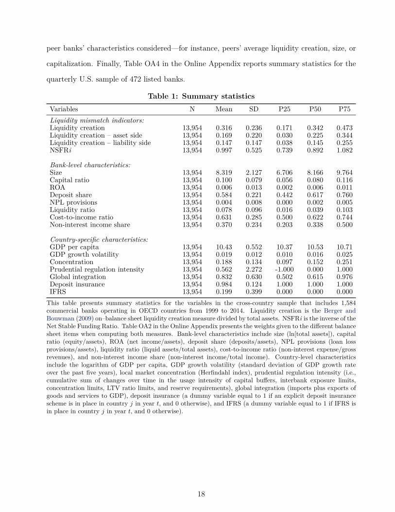
Summary Statistics. Table 1 reports descriptive statistics for the main variables in the
cross-country sample. The average bank is creating liquidity (0.316), both on the asset
(0.169) and liability (0.147) sides of the balance sheet. If in place, it would be complying
with the regulatory NSFR (100.3%). Bank-level characteristics include size (ln[total assets]),
capital ratio (equity/assets), ROA (net income/assets), deposit share (deposits/assets), NPL
provisions (loan loss provisions/assets), liquidity ratio (liquid assets/assets), cost-to-income
ratio (non-interest expense/gross revenues), and non-interest income share (non-interest income
/total income), all winsorized at the 1st and 99th percentile levels. Country-level characteristics
include the logarithm of GDP per capita, GDP growth volatility (standard deviation of GDP
growth rate over the past five years), local market concentration (Herfindahl index), the
Cerutti, Correa, Fiorentino, and Segalla (2017) prudential regulation intensity measure, global
integration (imports plus exports of goods and services to GDP), deposit insurance (a dummy
variable equal to 1 if an explicit deposit insurance scheme is in place in country j in year t,
and 0 otherwise), and IFRS (a dummy variable equal to 1 if IFRS is in place in country j
in year t, and 0 otherwise) to account for potential reporting jumps at the time of a bank’s
accounting standards change. The bank- and country-level controls are comparable in terms
of magnitude to those in previous studies consistently showing their importance for banks’
financial decisions (e.g., Beltratti and Stulz, 2012; Beck, De Jonghe, and Schepens, 2013).
For completeness, Table OA3 in the Online Appendix presents summary statistics for all the
16I first verify that I match the values reported by Bai, Krishnamurthy, and Weymuller (2018) when usingFRY-9C. The weights are not affected by business models and, as a result, the LMI can be applied to eitherbank holding companies or commercial banks. The detailed description of how to construct the LMI is providedin Appendix I of Bai, Krishnamurthy, and Weymuller (2018). The repo haircut data is collected from the SECEdgar website until 2010 and the FRB of New York since 2010:Q1. The secondary loan market haircuts arefrom the Loan Syndications & Trading Association. The OIS and Treasury bill data are from Bloomberg.
17
peer banks’ characteristics considered—for instance, peers’ average liquidity creation, size, or
capitalization. Finally, Table OA4 in the Online Appendix reports summary statistics for the
quarterly U.S. sample of 472 listed banks.
Table 1: Summary statisticsVariables N Mean SD P25 P50 P75Liquidity mismatch indicators:Liquidity creation 13,954 0.316 0.236 0.171 0.342 0.473Liquidity creation – asset side 13,954 0.169 0.220 0.030 0.225 0.344Liquidity creation – liability side 13,954 0.147 0.147 0.038 0.145 0.255NSFRi 13,954 0.997 0.525 0.739 0.892 1.082
Bank-level characteristics:Size 13,954 8.319 2.127 6.706 8.166 9.764Capital ratio 13,954 0.100 0.079 0.056 0.080 0.116ROA 13,954 0.006 0.013 0.002 0.006 0.011Deposit share 13,954 0.584 0.221 0.442 0.617 0.760NPL provisions 13,954 0.004 0.008 0.000 0.002 0.005Liquidity ratio 13,954 0.078 0.096 0.016 0.039 0.103Cost-to-income ratio 13,954 0.631 0.285 0.500 0.622 0.744Non-interest income share 13,954 0.370 0.234 0.203 0.338 0.500
Country-specific characteristics:GDP per capita 13,954 10.43 0.552 10.37 10.53 10.71GDP growth volatility 13,954 0.019 0.012 0.010 0.016 0.025Concentration 13,954 0.188 0.134 0.097 0.152 0.251Prudential regulation intensity 13,954 0.562 2.272 -1.000 0.000 1.000Global integration 13,954 0.832 0.630 0.502 0.615 0.976Deposit insurance 13,954 0.984 0.124 1.000 1.000 1.000IFRS 13,954 0.199 0.399 0.000 0.000 0.000
This table presents summary statistics for the variables in the cross-country sample that includes 1,584commercial banks operating in OECD countries from 1999 to 2014. Liquidity creation is the Berger andBouwman (2009) on–balance sheet liquidity creation measure divided by total assets. NSFRi is the inverse of theNet Stable Funding Ratio. Table OA2 in the Online Appendix presents the weights given to the different balancesheet items when computing both measures. Bank-level characteristics include size (ln[total assets]), capitalratio (equity/assets), ROA (net income/assets), deposit share (deposits/assets), NPL provisions (loan lossprovisions/assets), liquidity ratio (liquid assets/total assets), cost-to-income ratio (non-interest expense/grossrevenues), and non-interest income share (non-interest income/total income). Country-level characteristicsinclude the logarithm of GDP per capita, GDP growth volatility (standard deviation of GDP growth rateover the past five years), local market concentration (Herfindahl index), prudential regulation intensity (i.e.,cumulative sum of changes over time in the usage intensity of capital buffers, interbank exposure limits,concentration limits, LTV ratio limits, and reserve requirements), global integration (imports plus exports ofgoods and services to GDP), deposit insurance (a dummy variable equal to 1 if an explicit deposit insurancescheme is in place in country j in year t, and 0 otherwise), and IFRS (a dummy variable equal to 1 if IFRS isin place in country j in year t, and 0 otherwise).
18

4 Results
4.1 Peer Effects in Banks’ Liquidity Mismatch Decisions
Baseline Results. Table 2 reports the benchmark set of results examining whether the
liquidity mismatch decisions of a specific bank are determined by the respective choices of
its competitors. The table presents 2SLS coefficient estimates of Model (1) using the Berger
and Bouwman (2009) liquidity creation measure as the dependent variable and, exploiting
the presence of partially overlapping peer groups, the liquidity policy of “peers of peers” as
a relevant instrument (Bramoulle, Djebbari, and Fortin, 2009). The row at the top of the
table reports the peer effect of interest—that is, the estimated coefficient on the instrumented
peer banks’ average liquidity creation. Peer groups are defined as commercial banks operating
in the same country in the same year grouped into a maximum of 10 (Columns 1–2), 20
(Columns 3–4), and 30 banks (Columns 5–6) according to their size. The regressions in
Columns (1), (3), and (5) control for the standard set of bank, peer average, and country
characteristics used throughout the paper, while those in Columns (2), (4), and (6) include
additional covariates to minimize omitted variable concerns. All specifications include year
and bank fixed effects, and the t-statistics in parentheses are robust to heteroskedasticity and
within-peer-group dependence.17
Consistent with the theoretical predictions of Farhi and Tirole (2012) and Albuquerque,
Cabral, and Guedes (2019), among others, the results across all specifications in Table 2 show
that the liquidity created by individual banks is significantly and positively affected by the
liquidity transformation activity of the respective competitors. To ease the interpretation of
magnitudes and ensure comparability across different samples, all coefficients are scaled by
17Following the example in Figure 1, the peer group that includes Banks C1–C4 constitutes the relevantcluster to build inference since there is no variation in the instrument across them. In other words, given thatthe liquidity created by Bank X (the foreign parent bank holding group that owns the foreign subsidiary A)should be positively correlated with that of C1, C2, C3, and C4 through the effect on A’s liquidity creation,and since banks C1–C4 become identified using the characteristics of the same Bank X as an instrument,the standard errors should be clustered at the peer group level. While the results are robust to alternativeunits of clustering, clustering at the peer group level yields considerably more conservative standard errors andfirst-stage F-statistics—see Table OA5 in the Online Appendix.
19
the corresponding variable’s standard deviation. Thus, a one-standard-deviation increase in
peers’ average liquidity creation leads to a 5–9 percentage point increase in bank i’s liquidity
creation, corresponding to a 16–28% increase relative to the mean.18
While bank-specific liquidity mismatch decisions are mostly driven by direct responses to
the respective policies of competitors, some other peer characteristics such as their average
capital and non-interest revenue share also matter for its determination. Nevertheless, their
joint effect on individual banks’ liquidity decisions is economically small and not robust. This
suggests that (i) the results are not likely to be driven by shared characteristics between banks
and their respective peers, and that (ii) any bias due to omitted characteristics of competitors
that are relevant for bank i’s liquidity choices is likely to be small.
Identifying Assumptions. The relevance condition requires the IV to be significantly
correlated with peer banks’ average liquidity creation (the endogenous variable), and the results
in Table 2 show this is indeed the case. In fact, the instrument is always significant at the
1% level in the first stage of the 2SLS estimation in all specifications and the cluster-robust
Kleibergen and Paap (2006) F-statistic also rejects the hypothesis of a weak IV.
Together with the relevance condition, the exclusion restriction implies that the only role
the instrument plays in influencing the outcome variable is through its effect on the endogenous
variable. In other words, the identification strategy solves the endogeneity problem only if the
foreign parent bank holding group does not directly influence the liquidity mismatch decision
of a domestic bank i. Thus, the estimates may be biased if the liquidity created by the foreign
parent is correlated with either an omitted characteristic of peer banks that is relevant for
bank i’s liquidity policy, or an omitted bank i liquidity creation determinant. While the
results discussed above suggest a limited role of the former, the latter concern is addressed as
follows.
18The unscaled coefficient estimates can be retrieved by dividing each coefficient with the correspondingvariable’s standard deviation presented in Table OA3 in the Online Appendix. The results in Table OA6 showthat this effect is still statistically significant, though underestimated, when using OLS regressions.
20
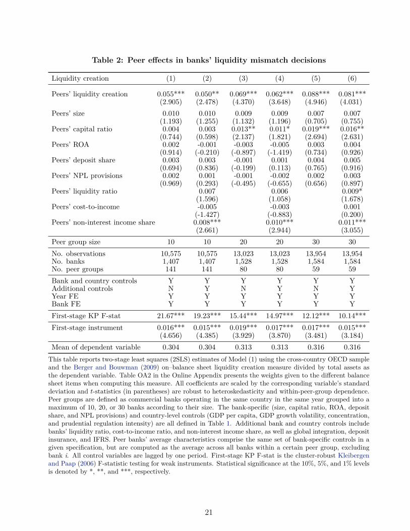
Table 2: Peer effects in banks’ liquidity mismatch decisions
Liquidity creation (1) (2) (3) (4) (5) (6)
Peers’ liquidity creation 0.055*** 0.050** 0.069*** 0.062*** 0.088*** 0.081***(2.905) (2.478) (4.370) (3.648) (4.946) (4.031)
Peers’ size 0.010 0.010 0.009 0.009 0.007 0.007(1.193) (1.255) (1.132) (1.196) (0.705) (0.755)
Peers’ capital ratio 0.004 0.003 0.013** 0.011* 0.019*** 0.016**(0.744) (0.598) (2.137) (1.821) (2.694) (2.631)
Peers’ ROA 0.002 -0.001 -0.003 -0.005 0.003 0.004(0.914) (-0.210) (-0.897) (-1.419) (0.734) (0.926)
Peers’ deposit share 0.003 0.003 -0.001 0.001 0.004 0.005(0.694) (0.836) (-0.199) (0.113) (0.765) (0.916)
Peers’ NPL provisions 0.002 0.001 -0.001 -0.002 0.002 0.003(0.969) (0.293) (-0.495) (-0.655) (0.656) (0.897)
Peers’ liquidity ratio 0.007 0.006 0.009*(1.596) (1.058) (1.678)
Peers’ cost-to-income -0.005 -0.003 0.001(-1.427) (-0.883) (0.200)
Peers’ non-interest income share 0.008*** 0.010*** 0.011***(2.661) (2.944) (3.055)
Peer group size 10 10 20 20 30 30No. observations 10,575 10,575 13,023 13,023 13,954 13,954No. banks 1,407 1,407 1,528 1,528 1,584 1,584No. peer groups 141 141 80 80 59 59Bank and country controls Y Y Y Y Y YAdditional controls N Y N Y N YYear FE Y Y Y Y Y YBank FE Y Y Y Y Y YFirst-stage KP F-stat 21.67*** 19.23*** 15.44*** 14.97*** 12.12*** 10.14***First-stage instrument 0.016*** 0.015*** 0.019*** 0.017*** 0.017*** 0.015***
(4.656) (4.385) (3.929) (3.870) (3.481) (3.184)Mean of dependent variable 0.304 0.304 0.313 0.313 0.316 0.316
This table reports two-stage least squares (2SLS) estimates of Model (1) using the cross-country OECD sampleand the Berger and Bouwman (2009) on–balance sheet liquidity creation measure divided by total assets asthe dependent variable. Table OA2 in the Online Appendix presents the weights given to the different balancesheet items when computing this measure. All coefficients are scaled by the corresponding variable’s standarddeviation and t-statistics (in parentheses) are robust to heteroskedasticity and within-peer-group dependence.Peer groups are defined as commercial banks operating in the same country in the same year grouped into amaximum of 10, 20, or 30 banks according to their size. The bank-specific (size, capital ratio, ROA, depositshare, and NPL provisions) and country-level controls (GDP per capita, GDP growth volatility, concentration,and prudential regulation intensity) are all defined in Table 1. Additional bank and country controls includebanks’ liquidity ratio, cost-to-income ratio, and non-interest income share, as well as global integration, depositinsurance, and IFRS. Peer banks’ average characteristics comprise the same set of bank-specific controls in agiven specification, but are computed as the average across all banks within a certain peer group, excludingbank i. All control variables are lagged by one period. First-stage KP F-stat is the cluster-robust Kleibergenand Paap (2006) F-statistic testing for weak instruments. Statistical significance at the 10%, 5%, and 1% levelsis denoted by *, **, and ***, respectively.
21
First, Columns (1) to (3) of Table 3 report the results of an extended version of Model
(1) with country×year fixed effects for country-year pairs with more than one peer group.
Despite being slightly smaller in magnitude, the estimated coefficients are still economically and
statistically significant, with estimates ranging from a 4 to 7 percentage point increase in bank
i’s liquidity creation following a one-standard-deviation increase in the liquidity created by its
competitors. This result corroborates the previous findings and helps ruling out alternative
explanations such as the effect being driven by changes in regulations or supervisory effort that
the model may not able to perfectly control for.
Second, to mitigate any remaining concerns that the results may still be biased due to
omitted time-varying bank characteristics, I apply the methodology developed by Altonji,
Elder, and Taber (2005) to quantify the relative importance of any remaining omitted variable
bias. Coefficient stability is computed as the ratio between each coefficient estimate including
controls as reported in Table 2 (numerator), and the difference between the latter and the
coefficient derived from a regression with the same number of observations but without any
controls (denominator). The results suggest that to explain the full effect of peers’ liquidity
creation, the covariance between unobserved factors and peers’ liquidity creation would have
to be between 10.09 to 58.58 times as high as the covariance of the included controls. In
comparison, Altonji, Elder, and Taber (2005) estimate a ratio of 3.55, which they interpret as
evidence that unobservables are unlikely to explain the effect they analyze. Accordingly, one
can conclude that the likelihood that unobserved heterogeneity explains the documented peer
effects is likely to be small.
Finally, the identifying assumption may still not be satisfied if the country where the foreign
parent bank holding company is headquartered and the country where the domestic banks
operate were subject to similar shocks that could influence the liquidity they both create. To
address this concern, I repeat the analysis with a modified IV that purges the common variation
in the baseline instrument. In detail, I first regress the liquidity created by the foreign parent
with observed country-level characteristics as well as country and time fixed effects. Then, the
22
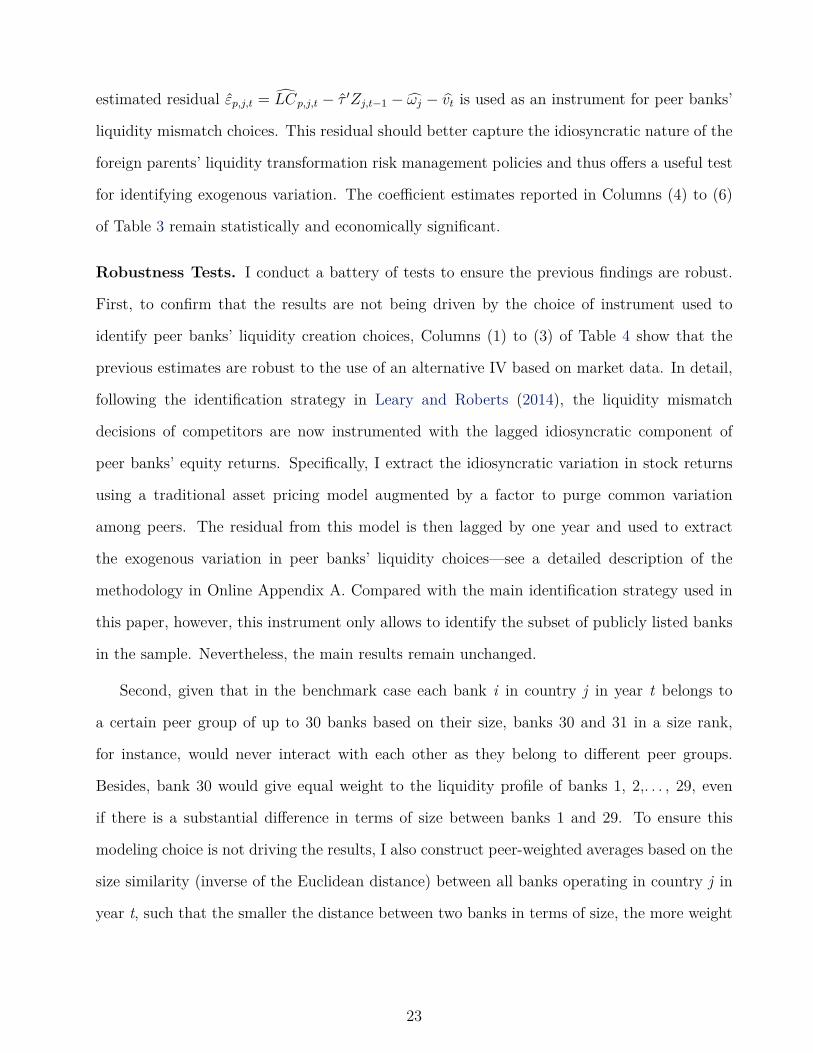
estimated residual εp,j,t = LCp,j,t − τ ′Zj,t−1 − ωj − vt is used as an instrument for peer banks’
liquidity mismatch choices. This residual should better capture the idiosyncratic nature of the
foreign parents’ liquidity transformation risk management policies and thus offers a useful test
for identifying exogenous variation. The coefficient estimates reported in Columns (4) to (6)
of Table 3 remain statistically and economically significant.
Robustness Tests. I conduct a battery of tests to ensure the previous findings are robust.
First, to confirm that the results are not being driven by the choice of instrument used to
identify peer banks’ liquidity creation choices, Columns (1) to (3) of Table 4 show that the
previous estimates are robust to the use of an alternative IV based on market data. In detail,
following the identification strategy in Leary and Roberts (2014), the liquidity mismatch
decisions of competitors are now instrumented with the lagged idiosyncratic component of
peer banks’ equity returns. Specifically, I extract the idiosyncratic variation in stock returns
using a traditional asset pricing model augmented by a factor to purge common variation
among peers. The residual from this model is then lagged by one year and used to extract
the exogenous variation in peer banks’ liquidity choices—see a detailed description of the
methodology in Online Appendix A. Compared with the main identification strategy used in
this paper, however, this instrument only allows to identify the subset of publicly listed banks
in the sample. Nevertheless, the main results remain unchanged.
Second, given that in the benchmark case each bank i in country j in year t belongs to
a certain peer group of up to 30 banks based on their size, banks 30 and 31 in a size rank,
for instance, would never interact with each other as they belong to different peer groups.
Besides, bank 30 would give equal weight to the liquidity profile of banks 1, 2,. . . , 29, even
if there is a substantial difference in terms of size between banks 1 and 29. To ensure this
modeling choice is not driving the results, I also construct peer-weighted averages based on the
size similarity (inverse of the Euclidean distance) between all banks operating in country j in
year t, such that the smaller the distance between two banks in terms of size, the more weight
23
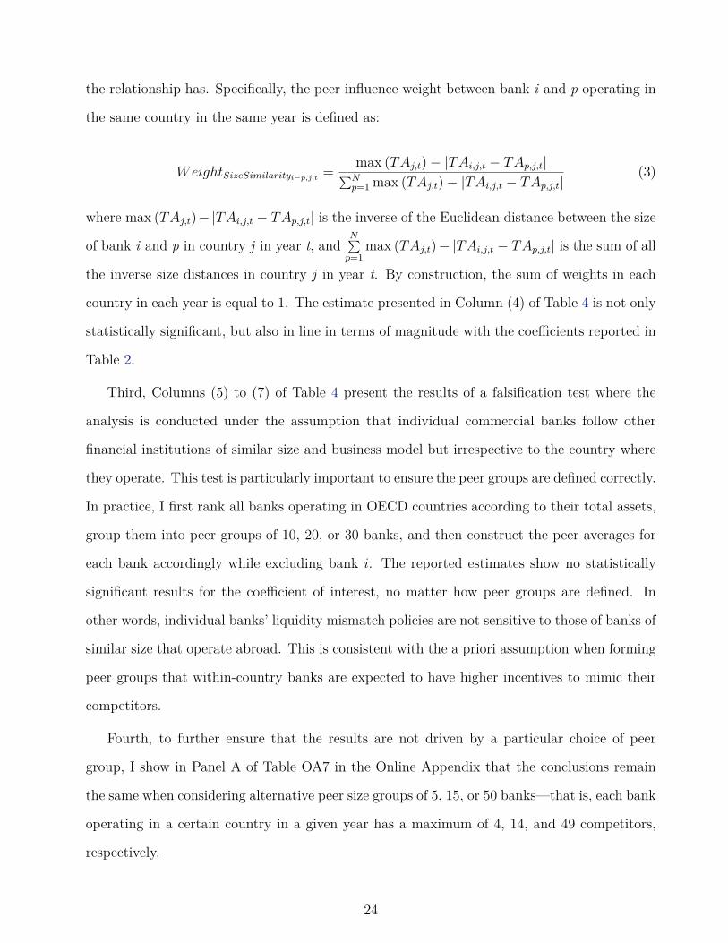
the relationship has. Specifically, the peer influence weight between bank i and p operating in
the same country in the same year is defined as:
WeightSizeSimilarityi−p,j,t= max (TAj,t)− |TAi,j,t − TAp,j,t|∑N
p=1 max (TAj,t)− |TAi,j,t − TAp,j,t|(3)
where max (TAj,t)−|TAi,j,t − TAp,j,t| is the inverse of the Euclidean distance between the size
of bank i and p in country j in year t, andN∑
p=1max (TAj,t)− |TAi,j,t − TAp,j,t| is the sum of all
the inverse size distances in country j in year t. By construction, the sum of weights in each
country in each year is equal to 1. The estimate presented in Column (4) of Table 4 is not only
statistically significant, but also in line in terms of magnitude with the coefficients reported in
Table 2.
Third, Columns (5) to (7) of Table 4 present the results of a falsification test where the
analysis is conducted under the assumption that individual commercial banks follow other
financial institutions of similar size and business model but irrespective to the country where
they operate. This test is particularly important to ensure the peer groups are defined correctly.
In practice, I first rank all banks operating in OECD countries according to their total assets,
group them into peer groups of 10, 20, or 30 banks, and then construct the peer averages for
each bank accordingly while excluding bank i. The reported estimates show no statistically
significant results for the coefficient of interest, no matter how peer groups are defined. In
other words, individual banks’ liquidity mismatch policies are not sensitive to those of banks of
similar size that operate abroad. This is consistent with the a priori assumption when forming
peer groups that within-country banks are expected to have higher incentives to mimic their
competitors.
Fourth, to further ensure that the results are not driven by a particular choice of peer
group, I show in Panel A of Table OA7 in the Online Appendix that the conclusions remain
the same when considering alternative peer size groups of 5, 15, or 50 banks—that is, each bank
operating in a certain country in a given year has a maximum of 4, 14, and 49 competitors,
respectively.
24
Fifth, while the identifying assumption that a foreign-owned subsidiary considers the
liquidity mismatch policy of its parent bank holding group (in addition to that of its domestic
peers) should in principle be more appropriate when the subsidiary is not too small or not
too large relative to its parent, the results reported in Panel B of Table OA7 in the Online
Appendix show that the conclusions remain the same if not restricting the size of the parents in
relation to their respective subsidiaries when computing the IV. Similarly, the results are also
robust to more stringent relative size restrictions. These include excluding foreign parent bank
holding groups in which their respective subsidiaries are more than 25% or less than 1% of the
parents’ size (when tightening the “too big” restriction in relation to the baseline case), and
excluding foreign parent bank holding groups in which their respective subsidiaries are more
than 50% or less than 10% of the parents’ size (when tightening the “too small” restriction in
relation to the baseline case).
Sixth, the conclusions do not change when considering the inverse of the NSFR (NSFRi) as
an alternative, though complementary, liquidity mismatch indicator—while liquidity creation
is an indicator of current illiquidity, the NSFR captures what illiquidity would be under a stress
scenario (Berger and Bouwman, 2015). Panel A of Table OA8 in the Online Appendix follows
the same structure of Table 2, and the reported 2SLS estimated coefficients corroborate the
previous findings: the first-stage regression coefficient estimates and the Kleibergen and Paap
(2006) F-statistic show that the instrument is relevant and not weak, and the estimates on
the coefficient of interest indicate that the relationship between the liquidity transformation
risk of individual banks and those of its peers is positive and statistically significant in all
specifications.
Finally, the main findings also remain unchanged (i) when excluding banks operating in
the United States, thus suggesting that such collective behavior is pervasive across OECD
countries, (ii) when excluding all foreign-owned subsidiaries from the estimations, (iii) when
using the lagged peer banks’ liquidity creation (instead of a contemporaneous measure) as the
main explanatory variable, (iv) without winsorizing any of the control variables, and (v) when
25
removing from the sample banks with asset growth above 75% in any of the years they are
active, since these may have been involved in mergers and acquisitions—see Tables OA8 and
OA9 in the Online Appendix.
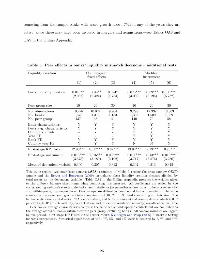
Table 3: Peer effects in banks’ liquidity mismatch decisions – additional tests
Liquidity creation Country-year Modifiedfixed effects instrument
(1) (2) (3) (4) (5) (6)
Peers’ liquidity creation 0.040** 0.044** 0.074* 0.076*** 0.089*** 0.103***(2.037) (2.424) (1.754) (3.030) (6.195) (5.732)
Peer group size 10 20 30 10 20 30No. observations 10,228 10,822 9,964 9,298 12,337 13,563No. banks 1,375 1,315 1,163 1,362 1,509 1,569No. peer groups 137 68 41 140 79 58Bank characteristics Y Y Y Y Y YPeers avg. characteristics Y Y Y Y Y YCountry controls - - - Y Y YYear FE - - - Y Y YBank FE Y Y Y Y Y YCountry-year FE Y Y Y N N NFirst-stage KP F-stat 12.80*** 10.17*** 9.62*** 13.82*** 12.79*** 10.76***First-stage instrument 0.013*** 0.016*** 0.008*** 0.011*** 0.013*** 0.013***
(3.578) (3.189) (3.102) (3.717) (3.576) (3.280)Mean of dependent variable 0.300 0.305 0.313 0.302 0.313 0.315
This table reports two-stage least squares (2SLS) estimates of Model (1) using the cross-country OECDsample and the Berger and Bouwman (2009) on–balance sheet liquidity creation measure divided bytotal assets as the dependent variable. Table OA2 in the Online Appendix presents the weights givento the different balance sheet items when computing this measure. All coefficients are scaled by thecorresponding variable’s standard deviation and t-statistics (in parentheses) are robust to heteroskedasticityand within-peer-group dependence. Peer groups are defined as commercial banks operating in the samecountry in the same year grouped into a maximum of 10, 20, or 30 banks according to their size. Thebank-specific (size, capital ratio, ROA, deposit share, and NPL provisions) and country-level controls (GDPper capita, GDP growth volatility, concentration, and prudential regulation intensity) are all defined in Table1. Peer banks’ average characteristics comprise the same set of bank-specific controls but are computed asthe average across all banks within a certain peer group, excluding bank i. All control variables are laggedby one period. First-stage KP F-stat is the cluster-robust Kleibergen and Paap (2006) F-statistic testingfor weak instruments. Statistical significance at the 10%, 5%, and 1% levels is denoted by *, **, and ***,respectively.
26

Tab
le4:
Pee
reff
ects
inba
nks’
liqui
dity
mis
mat
chde
cisi
ons
–ro
bust
ness
test
s
Liqu
idity
crea
tion
Alte
rnat
ive
Wei
ghte
dPe
ergr
oups
inst
rum
ent
peer
avg.
defin
edgl
obal
ly(1
)(2
)(3
)(4
)(5
)(6
)(7
)
Peer
s’liq
uidi
tycr
eatio
n0.
095*
**0.
086*
**0.
087*
**0.
091*
**0.
012
0.01
30.
037
(2.8
81)
(3.1
05)
(3.1
08)
(4.4
42)
(0.8
88)
(0.6
32)
(1.2
06)
Peer
grou
psiz
e10
2030
-10
2030
No.
obse
rvat
ions
2,98
32,
983
2,98
315
,418
11,8
3614
,502
15,1
79N
o.ba
nks
287
287
287
1,67
41,
407
1,52
81,
584
No.
peer
grou
ps34
2320
-12
664
43B
ank
char
acte
ristic
sY
YY
YY
YY
Peer
sav
g.ch
arac
teris
tics
YY
YY
YY
YC
ount
ryco
ntro
lsY
YY
YY
YY
Year
FEY
YY
YY
YY
Ban
kFE
YY
YY
YY
YFi
rst-
stag
eF-
stat
16.1
9***
24.3
1***
22.8
3***
116.
8***
17.8
4***
5.89
**1.
70Fi
rst-
stag
ein
stru
men
t0.
007*
**0.
008*
**0.
008*
**0.
015*
**0.
008*
**0.
005*
*0.
003
(4.0
23)
(4.9
30)
(4.7
78)
(10.
808)
(4.2
24)
(2.4
28)
(1.3
03)
Mea
nof
depe
nden
tva
riabl
e0.
389
0.38
90.
389
0.31
80.
321
0.32
20.
322
Thi
stab
lere
port
stw
o-st
age
leas
tsqu
ares
(2SL
S)es
timat
esof
Mod
el(1
)usin
gth
ecr
oss-
coun
try
OEC
Dsa
mpl
ean
dth
eB
erge
rand
Bou
wm
an(2
009)
on–b
alan
cesh
eet
liqui
dity
crea
tion
mea
sure
divi
ded
byto
tala
sset
sas
the
depe
nden
tva
riabl
e.Ta
ble
OA
2in
the
Onl
ine
App
endi
xpr
esen
tsth
ew
eigh
tsgi
ven
toth
edi
ffere
ntba
lanc
esh
eet
item
sw
hen
com
putin
gth
ism
easu
re.
All
coeffi
cien
tsar
esc
aled
byth
eco
rres
pond
ing
varia
ble’
ssta
ndar
dde
viat
ion
and
t-st
atist
ics(
inpa
rent
hese
s)ar
erob
ustt
ohe
tero
sked
astic
ityan
dw
ithin
bank
depe
nden
cein
Col
umns
(1)–
(4),
and
tohe
tero
sked
astic
ityan
dw
ithin
-pee
r-gr
oup
depe
nden
cein
Col
umns
(5)–
(7).
Peer
grou
psar
ede
fined
asco
mm
erci
alba
nks
oper
atin
gin
the
sam
eco
untr
yin
the
sam
eye
argr
oupe
din
toa
max
imum
of10
,20
,or
30ba
nks
acco
rdin
gto
thei
rsiz
e.T
heba
nk-s
peci
fic(s
ize,
capi
talr
atio
,RO
A,d
epos
itsh
are,
and
NPL
prov
ision
s)an
dco
untr
y-le
velc
ontr
ols
(GD
Ppe
rca
pita
,GD
Pgr
owth
vola
tility
,con
cent
ratio
n,an
dpr
uden
tialr
egul
atio
nin
tens
ity)
are
alld
efine
din
Tabl
e1.
Peer
bank
s’av
erag
ech
arac
teris
tics
com
prise
the
sam
ese
tof
bank
-spe
cific
cont
rols
but
are
com
pute
das
the
aver
age
acro
ssal
lban
ksw
ithin
ace
rtai
npe
ergr
oup,
excl
udin
gba
nki.
All
cont
rolv
aria
bles
are
lagg
edby
one
perio
d.Fi
rst-
stag
eK
PF-
stat
isth
ecl
uste
r-ro
bust
Kle
iber
gen
and
Paap
(200
6)F-
stat
istic
test
ing
for
wea
kin
stru
men
ts.
Stat
istic
alsig
nific
ance
atth
e10
%,5
%,a
nd1%
leve
lsis
deno
ted
by*,
**,a
nd**
*,re
spec
tivel
y.
27
U.S. Evidence. As a final robustness test, I reiterate the previous analysis when considering
a quarterly sample of banks operating in the United States. Restricting the analysis to this
panel of banks serves multiple purposes. First, using data from the Call Reports ensures that
the results are not driven by potential problems in Bankscope in terms of different definitions of
certain balance sheet categories across countries. Second, it preserves homogeneity in terms of
regulatory framework, accounting standards, and economic conditions. Third, it allows testing
whether the results on peer influence are sensitive to the use of higher frequency data. Finally,
since the information provided is considerably more granular, it also allows using the Berger
and Bouwman (2009) on– and off–balance sheet liquidity creation measure as the dependent
variable. The latter is particularly relevant given the extensive literature highlighting the
importance of off–balance sheet liquidity creation through loan commitments, standby letters
of credit, and other claims to liquid funds (e.g., Kashyap, Rajan, and Stein, 2002). In the
United States, for instance, this accounts for almost half of all liquidity created (Berger and
Bouwman, 2009).
In detail, Table 5 reports two-stage least squares estimates of Model (1) using both the
Berger and Bouwman (2009) on– and off–balance sheet (Columns 1–3) and on–balance sheet
(Columns 4–6) liquidity creation measures divided by total assets as the dependent variables.
Since there are no corresponding quarterly level data for most parents of foreign subsidiaries
operating in the United States, it is not possible to use here this paper’s main identification
strategy based on Bramoulle, Djebbari, and Fortin (2009) and De Giorgi, Pellizzari, and
Redaelli (2010). Besides, there are only a few small, mostly regional, foreign-owned subsidiaries
operating in the United States, which would not allow to identify a large portion of the domestic
banks in the sample. To counter this issue, I follow Leary and Roberts (2014) and, as in
Columns (1)–(3) of Table 4, use as IV the lagged peer bank average equity return shock.
In this case, standard errors are clustered at the bank level since the instrument varies across
banks and over time. The estimated coefficients are still significant as well as similar in terms of
magnitude across the liquidity creation measures with and without off–balance sheet exposures.
28

This suggests that peer banks have a negligible impact in the liquidity created by individual
banks off the balance sheet. I explore this hypothesis in detail in the next section.
Finally, Table 6 considers the Bai, Krishnamurthy, and Weymuller (2018) Liquidity Mismatch
Index (LMI) as the outcome variable. Despite relatively fewer observations when compared
with Table 5 due to the more granular nature of the data required to compute this measure
and since some of the market data is only available from 2002:Q2, the LMI has the advantage
of using liquidity weights that are time-varying with market liquidity conditions. The baseline
results still hold when considering this measure capturing the mismatch between the market
liquidity of assets and the funding liquidity of liabilities of a given bank—both its on– and
off–balance sheet (Columns 1–3) and on–balance sheet (Columns 4–6) versions.
4.2 Mechanisms and Heterogeneity
Asset versus Liability Side of Liquidity Creation. The results so far show that competitors
play a significant role in determining variations in liquidity mismatch policies of individual
banks. Nonetheless, peer influence can be concentrated or at least affect in a dissimilar way
liquidity created on the asset and liquidity sides of banks’ balance sheets. Berger, Bouwman,
Kick, and Schaeck (2016), for instance, show that capital support measures reduce banks’
asset-side liquidity creation while increasing by a similar magnitude the liquidity created on
the liability side. To better examine the mechanisms through which these adjustments operate,
I decompose aggregate liquidity creation into its individual elements (i.e., asset side, liability
side, and off–balance sheet liquidity creation—each divided by bank assets), and regress them
on peer banks’ corresponding component of liquidity creation.
The results reported in Tables 7 and OA10 indicate that peer effects are concentrated on
liquidity created on the asset side of banks’ balance sheets. Specifically, Table 7 considers
the cross-country OECD sample with annual frequency where the instrument is defined as the
foreign subsidiary’s parent asset or liability-side liquidity creation within each peer group. As
in Table 2, standard errors are robust to heteroskedasticity and within-peer-group dependence.
29
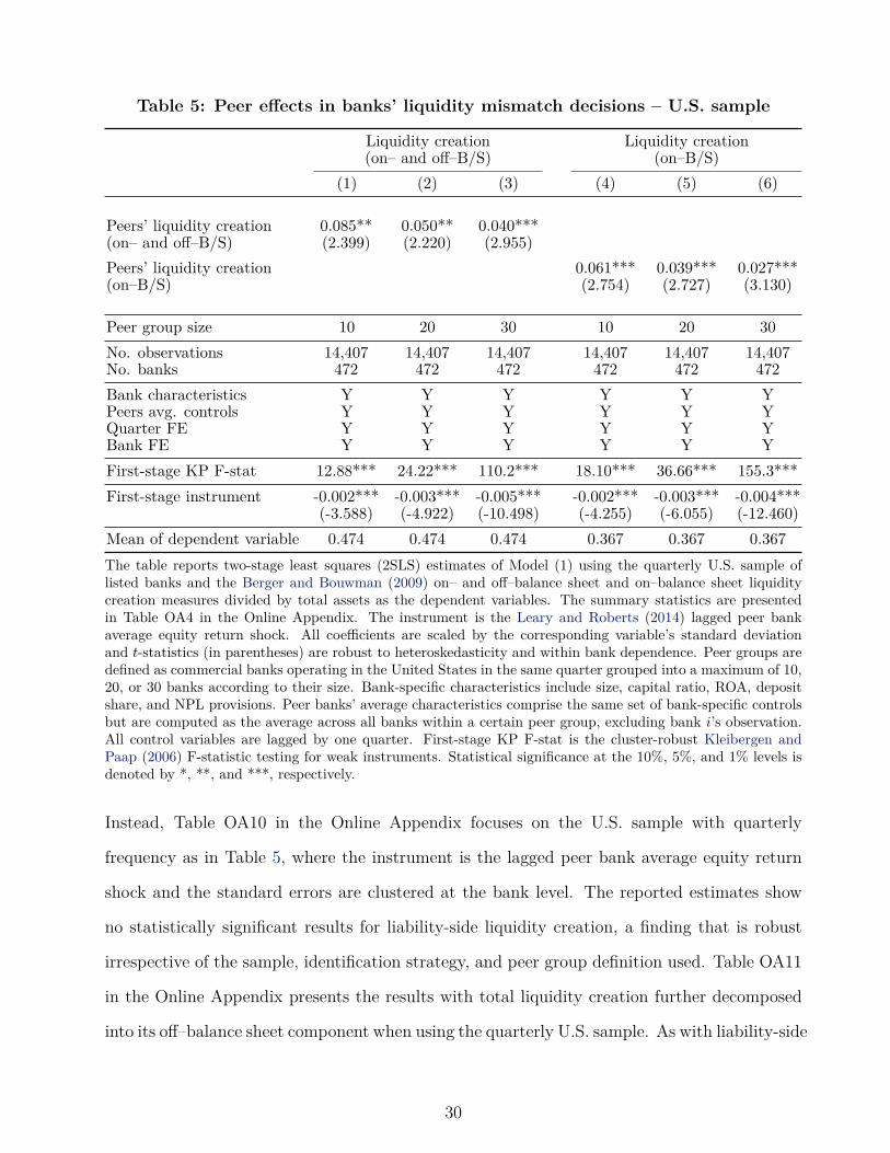
Table 5: Peer effects in banks’ liquidity mismatch decisions – U.S. sample
Liquidity creation Liquidity creation(on– and off–B/S) (on–B/S)
(1) (2) (3) (4) (5) (6)
Peers’ liquidity creation 0.085** 0.050** 0.040***(on– and off–B/S) (2.399) (2.220) (2.955)Peers’ liquidity creation 0.061*** 0.039*** 0.027***(on–B/S) (2.754) (2.727) (3.130)
Peer group size 10 20 30 10 20 30No. observations 14,407 14,407 14,407 14,407 14,407 14,407No. banks 472 472 472 472 472 472Bank characteristics Y Y Y Y Y YPeers avg. controls Y Y Y Y Y YQuarter FE Y Y Y Y Y YBank FE Y Y Y Y Y YFirst-stage KP F-stat 12.88*** 24.22*** 110.2*** 18.10*** 36.66*** 155.3***First-stage instrument -0.002*** -0.003*** -0.005*** -0.002*** -0.003*** -0.004***
(-3.588) (-4.922) (-10.498) (-4.255) (-6.055) (-12.460)Mean of dependent variable 0.474 0.474 0.474 0.367 0.367 0.367The table reports two-stage least squares (2SLS) estimates of Model (1) using the quarterly U.S. sample oflisted banks and the Berger and Bouwman (2009) on– and off–balance sheet and on–balance sheet liquiditycreation measures divided by total assets as the dependent variables. The summary statistics are presentedin Table OA4 in the Online Appendix. The instrument is the Leary and Roberts (2014) lagged peer bankaverage equity return shock. All coefficients are scaled by the corresponding variable’s standard deviationand t-statistics (in parentheses) are robust to heteroskedasticity and within bank dependence. Peer groups aredefined as commercial banks operating in the United States in the same quarter grouped into a maximum of 10,20, or 30 banks according to their size. Bank-specific characteristics include size, capital ratio, ROA, depositshare, and NPL provisions. Peer banks’ average characteristics comprise the same set of bank-specific controlsbut are computed as the average across all banks within a certain peer group, excluding bank i’s observation.All control variables are lagged by one quarter. First-stage KP F-stat is the cluster-robust Kleibergen andPaap (2006) F-statistic testing for weak instruments. Statistical significance at the 10%, 5%, and 1% levels isdenoted by *, **, and ***, respectively.
Instead, Table OA10 in the Online Appendix focuses on the U.S. sample with quarterly
frequency as in Table 5, where the instrument is the lagged peer bank average equity return
shock and the standard errors are clustered at the bank level. The reported estimates show
no statistically significant results for liability-side liquidity creation, a finding that is robust
irrespective of the sample, identification strategy, and peer group definition used. Table OA11
in the Online Appendix presents the results with total liquidity creation further decomposed
into its off–balance sheet component when using the quarterly U.S. sample. As with liability-side
30
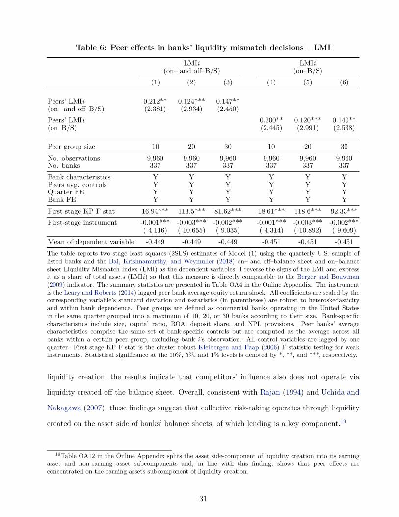
Table 6: Peer effects in banks’ liquidity mismatch decisions – LMI
LMIi LMIi(on– and off–B/S) (on–B/S)
(1) (2) (3) (4) (5) (6)
Peers’ LMIi 0.212** 0.124*** 0.147**(on– and off–B/S) (2.381) (2.934) (2.450)Peers’ LMIi 0.200** 0.120*** 0.140**(on–B/S) (2.445) (2.991) (2.538)
Peer group size 10 20 30 10 20 30No. observations 9,960 9,960 9,960 9,960 9,960 9,960No. banks 337 337 337 337 337 337Bank characteristics Y Y Y Y Y YPeers avg. controls Y Y Y Y Y YQuarter FE Y Y Y Y Y YBank FE Y Y Y Y Y YFirst-stage KP F-stat 16.94*** 113.5*** 81.62*** 18.61*** 118.6*** 92.33***First-stage instrument -0.001*** -0.003*** -0.002*** -0.001*** -0.003*** -0.002***
(-4.116) (-10.655) (-9.035) (-4.314) (-10.892) (-9.609)Mean of dependent variable -0.449 -0.449 -0.449 -0.451 -0.451 -0.451The table reports two-stage least squares (2SLS) estimates of Model (1) using the quarterly U.S. sample oflisted banks and the Bai, Krishnamurthy, and Weymuller (2018) on– and off–balance sheet and on–balancesheet Liquidity Mismatch Index (LMI) as the dependent variables. I reverse the signs of the LMI and expressit as a share of total assets (LMIi) so that this measure is directly comparable to the Berger and Bouwman(2009) indicator. The summary statistics are presented in Table OA4 in the Online Appendix. The instrumentis the Leary and Roberts (2014) lagged peer bank average equity return shock. All coefficients are scaled by thecorresponding variable’s standard deviation and t-statistics (in parentheses) are robust to heteroskedasticityand within bank dependence. Peer groups are defined as commercial banks operating in the United Statesin the same quarter grouped into a maximum of 10, 20, or 30 banks according to their size. Bank-specificcharacteristics include size, capital ratio, ROA, deposit share, and NPL provisions. Peer banks’ averagecharacteristics comprise the same set of bank-specific controls but are computed as the average across allbanks within a certain peer group, excluding bank i’s observation. All control variables are lagged by onequarter. First-stage KP F-stat is the cluster-robust Kleibergen and Paap (2006) F-statistic testing for weakinstruments. Statistical significance at the 10%, 5%, and 1% levels is denoted by *, **, and ***, respectively.
liquidity creation, the results indicate that competitors’ influence also does not operate via
liquidity created off the balance sheet. Overall, consistent with Rajan (1994) and Uchida and
Nakagawa (2007), these findings suggest that collective risk-taking operates through liquidity
created on the asset side of banks’ balance sheets, of which lending is a key component.19
19Table OA12 in the Online Appendix splits the asset side-component of liquidity creation into its earningasset and non-earning asset subcomponents and, in line with this finding, shows that peer effects areconcentrated on the earning assets subcomponent of liquidity creation.
31
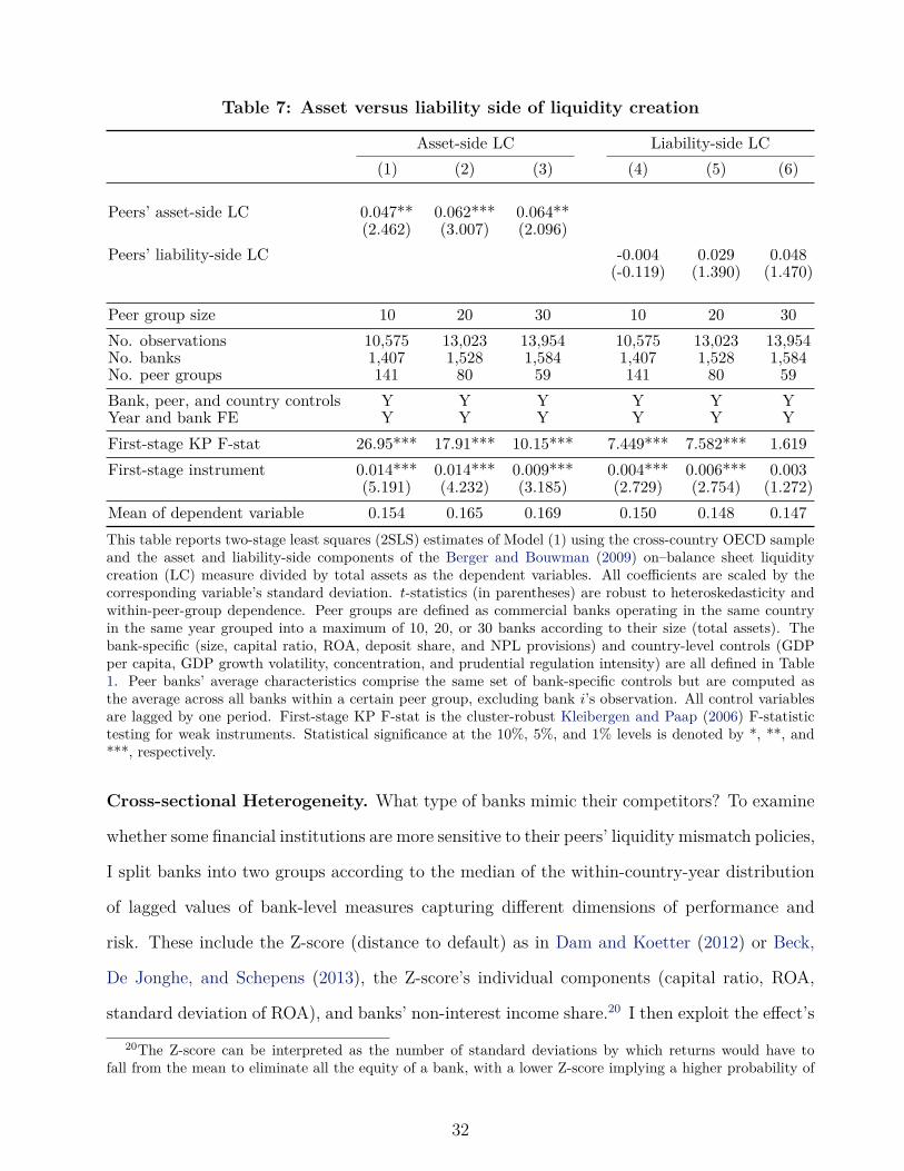
Table 7: Asset versus liability side of liquidity creation
Asset-side LC Liability-side LC(1) (2) (3) (4) (5) (6)
Peers’ asset-side LC 0.047** 0.062*** 0.064**(2.462) (3.007) (2.096)
Peers’ liability-side LC -0.004 0.029 0.048(-0.119) (1.390) (1.470)
Peer group size 10 20 30 10 20 30No. observations 10,575 13,023 13,954 10,575 13,023 13,954No. banks 1,407 1,528 1,584 1,407 1,528 1,584No. peer groups 141 80 59 141 80 59Bank, peer, and country controls Y Y Y Y Y YYear and bank FE Y Y Y Y Y YFirst-stage KP F-stat 26.95*** 17.91*** 10.15*** 7.449*** 7.582*** 1.619First-stage instrument 0.014*** 0.014*** 0.009*** 0.004*** 0.006*** 0.003
(5.191) (4.232) (3.185) (2.729) (2.754) (1.272)Mean of dependent variable 0.154 0.165 0.169 0.150 0.148 0.147This table reports two-stage least squares (2SLS) estimates of Model (1) using the cross-country OECD sampleand the asset and liability-side components of the Berger and Bouwman (2009) on–balance sheet liquiditycreation (LC) measure divided by total assets as the dependent variables. All coefficients are scaled by thecorresponding variable’s standard deviation. t-statistics (in parentheses) are robust to heteroskedasticity andwithin-peer-group dependence. Peer groups are defined as commercial banks operating in the same countryin the same year grouped into a maximum of 10, 20, or 30 banks according to their size (total assets). Thebank-specific (size, capital ratio, ROA, deposit share, and NPL provisions) and country-level controls (GDPper capita, GDP growth volatility, concentration, and prudential regulation intensity) are all defined in Table1. Peer banks’ average characteristics comprise the same set of bank-specific controls but are computed asthe average across all banks within a certain peer group, excluding bank i’s observation. All control variablesare lagged by one period. First-stage KP F-stat is the cluster-robust Kleibergen and Paap (2006) F-statistictesting for weak instruments. Statistical significance at the 10%, 5%, and 1% levels is denoted by *, **, and***, respectively.
Cross-sectional Heterogeneity. What type of banks mimic their competitors? To examine
whether some financial institutions are more sensitive to their peers’ liquidity mismatch policies,
I split banks into two groups according to the median of the within-country-year distribution
of lagged values of bank-level measures capturing different dimensions of performance and
risk. These include the Z-score (distance to default) as in Dam and Koetter (2012) or Beck,
De Jonghe, and Schepens (2013), the Z-score’s individual components (capital ratio, ROA,
standard deviation of ROA), and banks’ non-interest income share.20 I then exploit the effect’s20The Z-score can be interpreted as the number of standard deviations by which returns would have to
fall from the mean to eliminate all the equity of a bank, with a lower Z-score implying a higher probability of
32
cross-sectional heterogeneity by interacting the main explanatory variable of interest, peers’
liquidity creation, with the two indicator variables (ILow and IHigh) associated with a given
bank-level measure. All models are estimated by 2SLS where the two endogenous variables
are the peer banks’ average liquidity creation interacted with the two indicator variables, and
the two instruments are the peers’ parents liquidity creation interacted with the same two
indicator variables—since each model now has two endogenous regressors, there are also two
excluded instruments and two separate first-stage models. To avoid redundancy, the results
reported are based on the benchmark peer group definition, where competitors are defined as
other commercial banks operating in the same country in the same year and grouped into a
local network of 20 banks according to their size.
The results reported in Table 8 show that the peer effects in banks’ liquidity mismatch
decisions are concentrated in banks that are ex ante riskier. Importantly, the two first-stage
regressions in each of the models also show that (i) the instruments are correlated with the
endogenous variables in a way that is consistent with what one would expect, and that (ii)
the estimates do not seem to suffer from a weak instruments problem, with F-statistics and
associated p-values computed following the procedure of Sanderson and Windmeijer (2016) to
check for weak instruments in settings with more than one endogenous variable. In detail,
this form of collective risk-taking behavior is not present in banks with ex ante higher profit
stability and lower probability of default. The peer effects of interest are also not statistically
significant for banks with higher capital ratios, a result consistent with theory showing that
high capital strengthens banks’ monitoring incentives (Mehran and Thakor, 2011) and lowers
asset-substitution moral hazard (Morrison and White, 2005). Similarly, in Albuquerque,
Cabral, and Guedes (2019) the incentive to use more relative performance evaluation and
thus invest in correlated projects leading to systemic risk also increases with bank leverage.
Finally, this finding also suggests that higher levels of funding liquidity risk are not being
default. In detail, the Z-score of bank i at time t is defined as the sum of return on assets (ROA) and the capitalratio (equity to assets), all divided by the standard deviation of the ROA using a three-year rolling window.This approach avoids the variation in Z-scores within banks over time to be exclusively driven by variation inlevels of profitability and capital. Furthermore, by not relying on the full sample period, the denominator isno longer computed over different window lengths for different banks.
33
compensated with higher capital ratios that could increase a bank’s probability of survival
during the crisis (Berger and Bouwman, 2013).
Bank Size and Coordinated Behavior. Table 9 examines in more detail the potential
channels driving the correlated balance sheet exposures. Specifically, banks are first classified as
small or large by splitting the within country-year distribution of banks’ total assets according
to the median. The peer averages are then constructed based on: (i) small banks mimicking
small banks and large banks mimicking large banks; or (ii) small banks mimicking large banks
and large banks mimicking small banks. This analysis is useful not only to shed light on
the potential mechanisms behind this type of coordinated behavior, but also to understand
whether these decisions are indeed likely to be strategic.
The results confirm that the size of competitors is a crucial determinant for individual
banks’ decision-making. Specifically, the coefficient estimates indicate that large and small
banks’ liquidity mismatch decisions are only sensitive to choices of their respective counterparts.21
In other words, as predicted by the theoretical literature on collective moral hazard due to the
LOLR bailout commitment (e.g., Acharya and Yorulmazer, 2007; Farhi and Tirole, 2012), larger
banks tend to mimic other larger banks, while smaller banks follow other smaller banks. The
results therefore suggest that learning (i.e., free-riding in information acquisition) is unlikely
to play a major role in this setting since small banks’ liquidity choices do not seem to be
affected by the respective decisions of large banks. This differs from the findings of Leary
and Roberts (2014) that consider a sample of listed non-financial firms in the United States
and show that peer firm relevance is driven by a leader-follower model in which small firms
are sensitive to large firms, but not vice versa. In contrast with other industries, however, the
institutional framework (e.g., existence of government guarantees) and regulatory environment
(e.g., strict regulations and guidelines on what the banks can and should do) of the banking21In specifications with only one endogenous regressor (e.g., Columns 1 and 3 of Table 9), the Sanderson
and Windmeijer (2016) F-statistic is equal to the Kleibergen and Paap (2006) F-statistic I report in Tables 2to 7. While the peer groups in Column (1) of Table 9 are defined in a different manner than in the baselineanalysis (that is, banks within a country-year pair split into two size groups, where each group can have anynumber of banks versus banks within a country-year pair grouped into groups of 10, 20, and 30 banks of similarsize), it is reassuring that the coefficient estimate is similar in magnitude to those in Table 2.
34
sector arguably make it less likely for rational “herding” driven by small banks’ uncertainty
regarding the optimal liquidity mismatch policy to occur.
Additionally, the estimate in Column (2) of Table 9 shows that such mimicking behavior
is relatively stronger among larger banks. This is consistent with large banks taking more risk
than small banks in equilibrium since they internalize that their decisions directly affect the
government’s optimal bailout policy (Davila and Walther, 2018), but also with risk-taking being
driven by the presence of RPE in compensation schemes that tends to be more prevalent in
larger banks (Ilic, Pisarov, and Schmidt, 2017; Albuquerque, Cabral, and Guedes, 2019).22 This
finding is particularly important given that the trade-off between liquidity creation and fragility
is most consequential for large banks that create the most liquidity (Berger and Bouwman,
2009).
4.3 Collective Risk-taking and Financial Sector Stability
Asymmetric Behavior. To investigate the impact peer effects may have on financial sector
stability, I start by examining whether the response of individual banks to the liquidity
mismatch choices of competitors is asymmetric. In other words, this analysis aims to understand
if this type of mimicking behavior is stronger when peers are increasing liquidity transformation
risk rather than decreasing it. In fact, if banks follow competitors with the same intensity when
they are decreasing and increasing risk, the impact of such coordinated behavior on financial
stability is likely to be small. To answer this question, I interact the main explanatory variable
as well as the instrument with (i) a dummy variable equal to 1 if peers’ average liquidity
creation decreased from periods t − 1 to t, a 0 otherwise; and (ii) a dummy variable equal to
1 if peers’ average liquidity creation increased from periods t− 1 to t, and 0 otherwise.
22Davila and Walther (2018) show theoretically that since risky choices by large banks also increase theimplicit bailout subsidy for the banking sector as a whole, small banks may also increase risk-taking beyondwhat they would optimally choose in the absence of large banks. In contrast, Bonfim and Kim (2019) findsmall banks actually decrease liquidity risk when large banks are increasing it, although this result is notconsistent across different specifications. Empirically, and after providing a rigorous econometric treatmentfor the endogeneity of peer effects, I find no consistent evidence of strategic spillovers to small banks. In fact,although positive in terms of magnitude, the coefficient estimate in Column 4 of Table 9 (capturing small banksmimicking large banks) is statistically insignificant from zero.
35

Tab
le8:
Cro
ss-s
ecti
onal
hete
roge
neit
y
Liqu
idity
crea
tion
Cap
ital
Profi
tabi
lity
Non
-inte
rest
Profi
tst
abili
tyD
istan
ceto
defa
ult
ratio
(RO
A)
inco
me
shar
e(-
sd[R
OA
])(Z
-sco
re)
(1)
(2)
(3)
(4)
(5)
Peer
s’LC×
I Low
0.08
1***
0.06
6***
0.06
8***
0.07
9***
0.08
2***
(4.0
66)
(3.5
52)
(3.6
32)
(4.0
93)
(4.1
61)
Peer
s’LC×
I Hig
h0.
041
0.07
8***
0.07
2***
0.02
80.
028
(1.5
67)
(2.9
78)
(2.8
02)
(0.7
60)
(0.8
67)
No.
obse
rvat
ions
13,0
2313
,023
13,0
239,
794
9,79
4N
o.ba
nks
1,52
81,
528
1,52
81,
290
1,29
0N
o.pe
ergr
oups
8080
8078
78B
ank,
peer
,and
coun
try
cont
rols
YY
YY
YYe
aran
dba
nkFE
YY
YY
YM
ean
ofde
pend
ent
varia
ble
0.31
30.
313
0.31
30.
323
0.32
3
Firs
t-st
age
regr
essi
ons
Peer
s’LC
Peer
s’LC
Peer
s’LC
Peer
s’LC
Peer
s’LC
Peer
s’LC
Peer
s’LC
Peer
s’LC
Peer
s’LC
Peer
s’LC
×I L
ow
×I H
igh
×I L
ow
×I H
igh
×I L
ow
×I H
igh
×I L
ow
×I H
igh
×I L
ow
×I H
igh
(1.1
)(1
.2)
(2.1
)(2
.2)
(3.1
)(3
.2)
(4.1
)(4
.2)
(5.1
)(5
.2)
Firs
t-st
age
inst
rum
ent
1:0.
018*
**0.
000
0.01
8***
0.00
00.
018*
**0.
000
0.01
8***
0.00
00.
018*
**0.
000
Peer
s’pa
rent
sLC×
I Low
(4.2
93)
(0.1
02)
(3.9
00)
(0.0
24)
(4.1
63)
(0.0
51)
(3.7
87)
(0.2
02)
(3.6
60)
(0.2
19)
Firs
t-st
age
inst
rum
ent
2:-0
.002
0.02
1***
0.00
30.
017*
**-0
.001
0.02
2***
0.00
00.
015*
*0.
000
0.01
6**
Peer
s’pa
rent
sLC×
I Hig
h(-
0.41
4)(2
.979
)(0
.614
)(3
.047
)(-
0.23
9)(3
.139
)(0
.022
)(2
.311
)(0
.020
)(2
.551
)Fi
rst-
stag
eSW
F-St
at18
.49*
**10
.49*
**16
.00*
**13
.58*
**17
.33*
**12
.23*
**14
.70*
**9.
68**
*13
.86*
**11
.67*
**
Thi
sta
ble
repo
rts
two-
stag
ele
ast
squa
res
(2SL
S)es
timat
esof
Mod
el(1
)us
ing
the
cros
s-co
untr
yO
ECD
sam
ple
and
the
Ber
ger
and
Bou
wm
an(2
009)
on–b
alan
cesh
eetl
iqui
dity
crea
tion
mea
sure
(LC
)div
ided
byto
tala
sset
sast
hede
pend
entv
aria
ble.
Tabl
eO
A2
inth
eO
nlin
eA
ppen
dix
pres
ents
the
wei
ghts
give
nto
the
diffe
rent
bala
nce
shee
tite
ms
whe
nco
mpu
ting
this
mea
sure
.B
anks
are
split
into
two
grou
ps(I
Lo
wan
dI H
igh)
acco
rdin
gto
the
med
ian
ofth
ew
ithin
-cou
ntry
-yea
rdi
strib
utio
nof
lagg
edva
lues
ofba
nks’
capi
talr
atio
(equ
ity/a
sset
s),R
OA
(net
inco
me/
asse
ts),
non-
inte
rest
inco
me
shar
e(n
on-in
tere
stin
com
e/to
tali
ncom
e),
profi
tst
abili
ty(s
tand
ard
devi
atio
nof
the
RO
Aus
ing
ath
ree-
year
rolli
ngw
indo
w),
and
dist
ance
tode
faul
t(Z
-sco
re).
Toav
oid
redu
ndan
cy,
the
resu
ltsre
port
edar
eba
sed
onth
ebe
nchm
ark
peer
grou
pde
finiti
onas
insp
ecifi
catio
n(3
)of
Tabl
e2
whe
reco
mpe
titor
sar
ede
fined
asot
her
com
mer
cial
bank
sop
erat
ing
inth
esa
me
coun
try
inth
esa
me
year
,and
grou
ped
into
ane
twor
kof
20ba
nks
acco
rdin
gto
thei
rsiz
e.A
llco
effici
ents
are
scal
edby
the
corr
espo
ndin
gva
riabl
e’s
stan
dard
devi
atio
nan
dt-
stat
istic
s(in
pare
nthe
ses)
are
robu
stto
hete
rosk
edas
ticity
and
with
in-p
eer-
grou
pde
pend
ence
.Pe
ergr
oups
are
defin
edas
com
mer
cial
bank
sop
erat
ing
inth
esa
me
coun
try
inth
esa
me
year
grou
ped
into
am
axim
umof
10,2
0,or
30ba
nks
acco
rdin
gto
thei
rsiz
e.T
heba
nk-s
peci
fic(s
ize,
capi
talr
atio
,RO
A,d
epos
itsh
are,
and
NPL
prov
ision
s)an
dco
untr
y-le
velc
ontr
ols
(GD
Ppe
rca
pita
,GD
Pgr
owth
vola
tility
,con
cent
ratio
n,an
dpr
uden
tialr
egul
atio
nin
tens
ity)
are
alld
efine
din
Tabl
e1.
Peer
bank
s’av
erag
ech
arac
teris
tics
com
prise
the
sam
ese
tof
bank
-spe
cific
cont
rols
ina
give
nsp
ecifi
catio
n,bu
tar
eco
mpu
ted
asth
eav
erag
eac
ross
allb
anks
with
ina
cert
ain
peer
grou
p,ex
clud
ing
bank
i.A
llco
ntro
lvar
iabl
esar
ela
gged
byon
epe
riod.
Firs
t-st
age
SWF-
stat
isth
eSa
nder
son
and
Win
dmei
jer
(201
6)co
nditi
onal
first
-sta
geF-
stat
istic
test
ing
for
wea
kin
stru
men
ts.
Stat
istic
alsig
nific
ance
atth
e10
%,5
%,a
nd1%
leve
lsis
deno
ted
by*,
**,a
nd**
*,re
spec
tivel
y.
36

Table 9: Bank size and coordinated behavior
Liquidity creation Small → small Small → large& large → large & large → small
(1) (2) (3) (4)
Peers’ LC 0.084*** 0.035(6.380) (1.392)
Peers’ LC × ISmall 0.076*** 0.015(3.942) (0.275)
Peers’ LC × ILarge 0.093*** 0.055(5.653) (0.818)
No. observations 14,099 14,099 14,202 14,202No. banks 1,587 1,587 1,601 1,601No. peer groups 60 60 60 60Bank, peer, and country controls Y Y Y YYear and bank FE Y Y Y YMean of dependent variable 0.310 0.310 0.312 0.312
First-stage regressions Peers’ Peers’ Peers’ Peers’ Peers’ Peers’LC LC × LC × LC LC × LC ×
ISmall ILarge ISmall ILarge
(1.1) (2.1) (2.2) (3.1) (4.1) (4.2)First-stage intrument: 0.026*** 0.006Peers’ parents LC (5.281) (1.397)First-stage instrument 1: 0.020*** 0.003 0.008 0.002Peers’ parents LC × ISmall (3.936) (1.157) (1.561) (0.676)First-stage instrument 2: 0.004 0.027*** -0.001 0.001Peers’ parents LC × ILarge (0.983) (3.279) (-0.327) (0.238)First-stage SW F-Stat 27.89*** 16.75*** 10.06*** 1.951 0.114 0.076This table reports two-stage least squares (2SLS) estimates of Model (1) using the cross-country OECD sampleand the Berger and Bouwman (2009) on–balance sheet liquidity creation measure (LC) divided by total assets asthe dependent variable. Table OA2 in the Online Appendix presents the weights given to the different balancesheet items when computing this measure. Banks are split into two groups (ISmall and ILarge) accordingto the median of the within-country-year distribution of banks’ total assets. The peer averages are thenconstructed based on: (i) small banks mimicking small banks and large banks mimicking large banks; or (ii)small banks mimicking large banks and large banks mimicking small banks. All coefficients are scaled by thecorresponding variable’s standard deviation and t-statistics (in parentheses) are robust to heteroskedasticity andwithin-peer-group dependence. The bank-specific (size, capital ratio, ROA, deposit share, and NPL provisions)and country-level controls (GDP per capita, GDP growth volatility, concentration, and prudential regulationintensity) are all defined in Table 1. Peer banks’ average characteristics comprise the same set of bank-specificcontrols in a given specification, but are computed as the average across all banks within a certain peer group,excluding bank i. All control variables are lagged by one period. First-stage SW F-stat is the Sanderson andWindmeijer (2016) conditional first-stage F-statistic testing for weak instruments. Statistical significance atthe 10%, 5%, and 1% levels is denoted by *, **, and ***, respectively.
37
Table 10: Asymmetric behavior
Liquidity creation (1) (2) (3)
Peers’ LC × ILC↑ 0.069*** 0.086*** 0.104***(3.172) (4.109) (4.590)
Peers’ LC × ILC↓ 0.030 0.046 0.043(0.746) (1.630) (0.901)
No. observations 10,575 13,023 13,954No. banks 1,407 1,528 1,584No. peer groups 141 80 59Bank, peer, and country controls Y Y YYear and bank FE Y Y YMean of dependent variable 0.304 0.313 0.316
First-stage regressions Peers’ Peers’ Peers’ Peers’ Peers’ Peers’LC × LC × LC × LC × LC × LC ×ILC↑ ILC↓ ILC↑ ILC↓ ILC↑ ILC↓
(1.1) (1.2) (2.1) (2.2) (3.1) (3.2)First-stage instrument 1: 0.016*** -0.005 0.014** -0.001 0.016** -0.003Peers’ parents LC × ILC↑ (3.357) (-1.505) (2.504) (-0.346) (2.463) (-0.568)First-stage instrument 2: -0.000 0.016*** 0.001 0.019*** -0.000 0.017***Peers’ parents LC × ILC↓ (-0.006) (3.079) (0.189) (3.368) (-0.051) (2.862)First-stage SW F-Stat 16.96*** 17.18*** 10.19*** 17.08*** 8.39*** 14.99***This table reports two-stage least squares (2SLS) estimates of Model (1) using the cross-country OECD sampleand the Berger and Bouwman (2009) on–balance sheet liquidity creation measure (LC) divided by total assets asthe dependent variable. Table OA2 in the Online Appendix presents the weights given to the different balancesheet items when computing this measure. The main explanatory variable capturing the average liquiditycreated by competitors is interacted with (i) a dummy variable ILC↑ equal to 1 if peers’ average liquiditycreation increased from periods t-1 to t, a 0 otherwise; and (ii) a dummy variable ILC↓ equal to 1 if peers’average liquidity creation decreased from periods t-1 to t, and 0 otherwise. All coefficients are scaled by thecorresponding variable’s standard deviation and t-statistics (in parentheses) are robust to heteroskedasticity andwithin-peer-group dependence. The bank-specific (size, capital ratio, ROA, deposit share, and NPL provisions)and country-level controls (GDP per capita, GDP growth volatility, concentration, and prudential regulationintensity) are all defined in Table 1. Peer banks’ average characteristics comprise the same set of bank-specificcontrols in a given specification, but are computed as the average across all banks within a certain peer group,excluding bank i. All control variables are lagged by one period. First-stage SW F-stat is the Sanderson andWindmeijer (2016) conditional first-stage F-statistic testing for weak instruments. Statistical significance atthe 10%, 5%, and 1% levels is denoted by *, **, and ***, respectively.
Table 10 reports the findings. The results show that correlated liquidity transformation
activities do work asymmetrically, with individual banks mimicking their respective peers only
when competitors are increasing risk. Further validating the paper’s identification strategy,
the instruments are also correlated with the endogenous variables in the way one would expect:
38

while local banks behave strategically and mimic their respective peers only when competitors
are increasing liquidity creation, a foreign-owned subsidiary considers the liquidity mismatch
policy of its parent when the parent is both increasing and decreasing liquidity risk.23
Overall, the results suggest that banks’ liquidity policies are strategically determined
according to the behavior of their competitors, which can ultimately lead to financial instability
due to increased liquidity transformation risk in the banking system. Diamond and Rajan
(2001) and Allen and Gale (2004), for instance, argue that banks’ liquidity transformation
activities are a fundamental driver of fragility and suggest that bank failures are more likely to
occur when the level of liquidity creation is high. Rajan (1994) and Acharya and Naqvi (2012)
find that banks creating excessive liquidity also tend to engage in lending practices leading
to asset bubbles, which ultimately result in future financial instability. Berger and Bouwman
(2017) also show that banking crises in the United States have been preceded by periods of
abnormal liquidity creation. In a different context, Hong, Huang, and Wu (2014) show that
systemic liquidity risk as measured by TED spreads was a major predictor of bank failures in
2009 and 2010, while Cai, Eidam, Saunders, and Steffen (2018) analyze syndicated loans to
firms in the United States and show that a larger overlap of banks’ loan portfolio makes them
greater contributors to systemic risk and that interconnectedness increases aggregate systemic
risk during recessions.
Peer effects and Bank Risk. As a final step, I examine the consequences of strategic liquidity
mismatch choices explicitly—that is, whether such correlated balance sheet exposures have an
adverse effect on both individual banks’ default risk and overall systemic risk. Compared with
Model (1), the relationship between the liquidity mismatch position of bank i and that of
its peers is now allowed to vary not only across countries, but also over time following the23These findings also help to reassure that the baseline results are unlikely to be driven by changes in
prudential regulations introduced after the crisis or by the Basel’s first guidelines on the new liquidity regulationsissued in 2010. First, changes in the intensity of capital requirements, interbank exposure limits, concentrationlimits, LTV ratios limits, and reserve requirements are explicitly controlled for in the model following Cerutti,Correa, Fiorentino, and Segalla (2017). Second, these changes in regulation would imply that all banks adjusttheir portfolio towards reducing liquidity transformation risk. However, as the results in Table 10 show, suchcollective strategic behavior is asymmetric, with individual banks mimicking their respective peers only whencompetitors are increasing funding liquidity risk.
39

framework of Albuquerque, Cabral, and Guedes (2019) and Denbee, Julliard, Li, and Yuan
(2018). To capture time and country-varying peer effects in liquidity mismatch decisions, βj,t,
I shock the average peer effect in the overall sample with a country-year indicator variable Ij,t
and estimate the following model separately for each country-year combination:
yi,j,t = µi + (β0 + β1Ij,t)y−i,j,t + λ′X−i,j,t−1 + γ′Xi,j,t−1 + δ′Zj,t−1 + vt + εi,j,t (4)
where i, j, and t correspond to bank, country, and year, respectively.24 The estimated
coefficient on the peer effect of interest, βj,t, is then used to run the following specification
to gauge the impact of peer effects in liquidity choices on financial stability:
STAi,j,t = κ+ δβj,t + γ′Xi,j,t−1 + η′Zj,t−1 + µi + vt + ui,j,t (5)
where STAi,j,t is either the distance-to-default (ln[Z-score]) when using a three or five-year
window to compute the standard deviation of ROA, or the marginal expected shortfall—MES
(Acharya, Pedersen, Philippon, and Richardson, 2017) and systemic capital shortfall—SRISK
(Acharya, Engle, and Richardson, 2012; Brownlees and Engle, 2017). MES is computed using
the opposite of returns such that the higher a bank’s MES is, the higher its systemic risk
contribution. The market is defined as the country-specific banking sector equity market.
SRISK corresponds to the expected bank i’s capital shortage (in billion USD) during a period
of system distress and severe market decline. Following Acharya, Engle, and Richardson (2012),
the long-run MES is approximated as 1-exp(-18*MES) where MES is the one day loss expected
if market returns are less than -2%. Unlike MES, SRISK is a also function of the bank’s book
value of debt, its market value of equity and a minimum capital ratio. To ensure comparability
across countries, I follow Engle, Jondeau, and Rockinger (2015) and set the prudential capital
ratio to 4% for banks reporting under IFRS and to 8% for all other accounting standards,
including U.S. GAAP.
24For each of the separate regressions corresponding to each country-year combination Ij,t, there are againtwo endogenous regressors and two excluded instruments. I use the estimated coefficient on the peer effectfor a given country-year pair as a regressor to explain bank risk if and only if the Sanderson and Windmeijer(2016) conditional first-stage F-statistics are above the weak instrument critical values proposed by Stock andYogo (2005) based on size distortions of the associated Wald statistic considering a 25% maximal IV size.
40
The results reported in Tables OA13 and OA14 provide direct and thus novel empirical
evidence that strategic complementarity in banks’ liquidity mismatch policies decrease the
stability of the financial system. In fact, as initially hypothesized, the estimated coefficients
indicate that peer effects in liquidity mismatch policies are positively associated with individual
banks’ default risk and overall systemic risk. Importantly, this effect is both statistically
and economically significant. Irrespective of the multitude of channels that have been put
forward to explain this type of risk-taking behavior, these findings highlight the need of
having a macroprudential tool that minimizes the propensity for banks to create excessive
liquidity and collectively underprice liquidity risk. Such a binding requirement would allow for
more efficient systemic liquidity risk management that would ultimately reduce the potential
taxpayer burden.
5 Conclusion
The 2007–2009 financial crisis distinctly exposed the negative implications of excessive liquidity
transformation for financial sector stability and the macroeconomy. This outcome was achieved
in part through banks’ correlated exposures. Ultimately, liquidity mismatch decisions of
individual banks spilled over to other financial institutions and markets, exacerbating losses and
overall liquidity stress. Such systemic liquidity risk was, judging by the extent of government
intervention during the crisis, clearly understated by both the private and public sectors. In
this regard, this paper examines empirically the extent to which banks’ liquidity transformation
activities are affected by the choices of their competitors and the impact of these collective
risk-taking decisions on financial stability.
Using a novel identification strategy exploiting the presence of partially overlapping peer
groups, I show that financial institutions incorporate their peers’ liquidity mismatch decisions
when determining their own. This strategic behavior is driven by liquidity created on the
asset side, of which lending is a key component, and is concentrated in ex ante riskier banks.
With respect to the consequences of such strategic behavior for the financial system, I first
41
show that the response of individual banks to the liquidity mismatch choices of competitors
is asymmetric, with individual banks mimicking their peers only when competitors increase
liquidity transformation risk. I then show that peer effects in financial institutions’ liquidity
mismatch policies increase both individual banks’ default risk and overall systemic risk. This
effect is both statistically and economically significant, highlighting the importance of explicitly
regulating systemic liquidity risk from a macroprudential perspective.
In fact, while the Basel III liquidity requirements, combined with improved supervision,
should help to strengthen individual banks’ funding structure and thus enhance banking sector
stability, these liquidity standards are fundamentally microprudential in nature.25 Despite the
proposals for macroprudential liquidity regulation such as time-varying LCR and NSFR ratios
or a macroprudential liquidity buffer where each bank would be required to hold assets that are
systemically-liquid (IMF, 2011), policymakers and regulators have yet to establish a concise
macroprudential framework that mitigates the possibility of a simultaneous liquidity need by
financial institutions. Since information spillovers are a defining characteristic of panics due to
financial agents’ imperfect knowledge regarding common exposures and given that, as shown
in this paper, these information spillovers between banks do occur, a static and time-invariant
microprudential liquidity requirement that mainly depends on individual banks’ idiosyncratic
risk (rather than system-wide conditions) may not be suitable to prevent a systemic liquidity
crisis. As argued by Dewatripont, Rochet, and Tirole (2010), “a 1 percent probability of
failure means either that 1 percent of the banks fail every year or, alternatively, that the whole
banking system fails every hundred years—quite distinct outcomes. Therefore it is crucial for
regulators to find ways of discouraging herding behavior by banks.”
25Most developed economies have recently introduced formal bank bail-in regimes that involve theparticipation of bank creditors in bearing the costs of restoring a distressed bank and that include heavyrestrictions on taxpayer support. Despite the potentially negative but limited short-term costs of bail-ins forthe real economy (Beck, Da-Rocha-Lopes, and Silva, 2018), this new resolution tool represents an important stepto mitigate the incentives for collective risk-taking behavior. On the other hand, while the Financial StabilityBoard (FSB) issued in 2009 the core principles for the design of pay structures currently being implemented indifferent countries, Albuquerque, Cabral, and Guedes (2019) argue that these largely omit the role RPE playsin creating systemic risk.
42
ReferencesAcharya, V. V., Engle, R., Richardson, M., 2012. Capital shortfall: A new approach to ranking
and regulating systemic risks. The American Economic Review 102 (3), 59–64.Acharya, V. V., Mehran, H., Thakor, A. V., 2016. Caught between scylla and charybdis?
regulating bank leverage when there is rent seeking and risk shifting. Review of CorporateFinance Studies 5 (1), 36–75.
Acharya, V. V., Naqvi, H., 2012. The seeds of a crisis: A theory of bank liquidity and risktaking over the business cycle. Journal of Financial Economics 106 (2), 349–366.
Acharya, V. V., Pedersen, L. H., Philippon, T., Richardson, M., 2017. Measuring systemicrisk. The Review of Financial Studies 30 (1), 2–47.
Acharya, V. V., Thakor, A. V., 2016. The dark side of liquidity creation: Leverage and systemicrisk. Journal of Financial Intermediation 28, 4–21.
Acharya, V. V., Yorulmazer, T., 2007. Too many to fail - an analysis of time-inconsistency inbank closure policies. Journal of Financial Intermediation 16 (1), 1–31.
Acharya, V. V., Yorulmazer, T., 2008. Information contagion and bank herding. Journal ofMoney, Credit and Banking 40 (1), 215–231.
Albuquerque, A., 2009. Peer firms in relative performance evaluation. Journal of Accountingand Economics 48 (1), 69–89.
Albuquerque, R., Cabral, L., Guedes, J. C., 2019. Incentive pay and systemic risk. The Reviewof Financial Studies, forthcoming .
Allen, F., Babus, A., Carletti, E., 2012. Asset commonality, debt maturity and systemic risk.Journal of Financial Economics 104 (3), 519–534.
Allen, F., Gale, D., 2000. Financial contagion. Journal of Political Economy 108 (1), 1–33.Allen, F., Gale, D., 2004. Financial fragility, liquidity, and asset prices. Journal of the European
Economic Association 2 (6), 1015–1048.Allen, F., Gale, D., 2017. How should bank liquidity be regulated? Achieving Financial
Stability: Challenges To Prudential Regulation 61, 135.Altonji, J. G., Elder, T. E., Taber, C. R., 2005. Selection on observed and unobserved variables:
Assessing the effectiveness of catholic schools. Journal of Political Economy 113 (1), 151–184.Anginer, D., Cerutti, E., Martinez Peria, M. S., 2017. Foreign bank subsidiaries’ default risk
during the global crisis: What factors help insulate affiliates from their parents? Journal ofFinancial Intermediation 29, 19–31.
Bai, J., Krishnamurthy, A., Weymuller, C.-H., 2018. Measuring liquidity mismatch in thebanking sector. The Journal of Finance 73 (1), 51–93.
Banerjee, A. V., 1992. A simple model of herd behavior. The Quarterly Journal of Economics107 (3), 797–817.
BCBS, 2014. Basel III: The Net Stable Funding Ratio .Beck, T., Da-Rocha-Lopes, S., Silva, A. F., 2018. Sharing the pain? Credit supply and real
effects of bank bail-ins. Working Paper .Beck, T., De Jonghe, O., Schepens, G., 2013. Bank competition and stability: cross-country
heterogeneity. Journal of Financial Intermediation 22 (2), 218–244.
43
Beltratti, A., Stulz, R. M., 2012. The credit crisis around the globe: Why did some banksperform better? Journal of Financial Economics 105 (1), 1–17.
Bencivenga, V. R., Smith, B. D., 1991. Financial intermediation and endogenous growth. TheReview of Economic Studies 58 (2), 195–209.
Berger, A. N., Bouwman, C. H., 2009. Bank liquidity creation. The Review of Financial Studies22 (9), 3779–3837.
Berger, A. N., Bouwman, C. H., 2013. How does capital affect bank performance duringfinancial crises? Journal of Financial Economics 109 (1), 146–176.
Berger, A. N., Bouwman, C. H., 2015. Bank liquidity creation and financial crises. AcademicPress.
Berger, A. N., Bouwman, C. H., 2017. Bank liquidity creation, monetary policy, and financialcrises. Journal of Financial Stability 30, 139–155.
Berger, A. N., Bouwman, C. H., Kick, T., Schaeck, K., 2016. Bank liquidity creationfollowing regulatory interventions and capital support. Journal of Financial Intermediation26, 115–141.
Berger, A. N., Bouwman, C. H., Kim, D., 2017. Small bank comparative advantages inalleviating financial constraints and providing liquidity insurance over time. The Reviewof Financial Studies 30 (10), 3416–3454.
Berger, A. N., Sedunov, J., 2017. Bank liquidity creation and real economic output. Journalof Banking & Finance 81, 1–19.
Bikhchandani, S., Hirshleifer, D., Welch, I., 1998. Learning from the behavior of others:Conformity, fads, and informational cascades. The Journal of Economic Perspectives 12 (3),151–170.
Bizjak, J., Kalpathy, S. L., Li, Z. F., Young, B., 2018. The role of peer firm selection in explicitrelative performance awards. Working Paper .
Bizjak, J., Lemmon, M., Nguyen, T., 2011. Are all CEOs above average? An empiricalanalysis of compensation peer groups and pay design. Journal of Financial Economics 100 (3),538–555.
Blume, L. E., Brock, W. A., Durlauf, S. N., Jayaraman, R., 2015. Linear social interactionsmodels. Journal of Political Economy 123 (2), 444–496.
Bonfim, D., Kim, M., 2019. Liquidity risk and collective moral hazard. International Journalof Central Banking, forthcoming .
Bramoulle, Y., Djebbari, H., Fortin, B., 2009. Identification of peer effects through socialnetworks. Journal of Econometrics 150 (1), 41–55.
Brown, C. O., Dinc, I. S., 2011. Too many to fail? Evidence of regulatory forbearance whenthe banking sector is weak. The Review of Financial Studies 24 (4), 1378–1405.
Brownlees, C., Engle, R. F., 2017. SRISK: a conditional capital shortfall measure of systemicrisk. The Review of Financial Studies 30 (1), 48–79.
Brunnermeier, M. K., 2009. Deciphering the liquidity and credit crunch 2007–2008. The Journalof Economic Perspectives 23 (1), 77–100.
Cai, J., Eidam, F., Saunders, A., Steffen, S., 2018. Syndication, interconnectedness, andsystemic risk. Journal of Financial Stability 34, 105–120.
44
Calomiris, C. W., Heider, F., Hoerova, M., 2015. A theory of bank liquidity requirements.Columbia Business School Research Paper No. 14-39 .
Cerutti, E., Correa, R., Fiorentino, E., Segalla, E., 2017. Changes in prudential policyinstruments: A new cross-country database. International Journal of Central Banking13 (S1), 477–503.
Cetorelli, N., Goldberg, L. S., 2012a. Banking globalization and monetary transmission. TheJournal of Finance 67 (5), 1811–1843.
Cetorelli, N., Goldberg, L. S., 2012b. Liquidity management of US global banks: Internalcapital markets in the great recession. Journal of International Economics 88 (2), 299–311.
Claessens, S., Van Horen, N., 2015. The impact of the global financial crisis on bankingglobalization. IMF Economic Review 63 (4), 868–918.
Cornett, M. M., McNutt, J. J., Strahan, P. E., Tehranian, H., 2011. Liquidity risk managementand credit supply in the financial crisis. Journal of Financial Economics 101 (2), 297–312.
Dam, L., Koetter, M., 2012. Bank bailouts and moral hazard: Evidence from Germany. TheReview of Financial Studies 25 (8), 2343–2380.
Davila, E., Walther, A., 2018. Does size matter? Bailouts with large and small banks. NBERWorking Paper No. w24132 .
De Giorgi, G., Pellizzari, M., Redaelli, S., 2010. Identification of social interactions throughpartially overlapping peer groups. American Economic Journal: Applied Economics 2 (2),241–275.
Demirguc-Kunt, A., Kane, E., Laeven, L., 2015. Deposit insurance around the world: Acomprehensive analysis and database. Journal of Financial Stability 20, 155–183.
Denbee, E., Julliard, C., Li, Y., Yuan, K., 2018. Network risk and key players: A structuralanalysis of interbank liquidity. Working Paper .
Dewatripont, M., Rochet, J.-C., Tirole, J., 2010. Balancing the banks: Global lessons from thefinancial crisis. Princeton University Press.
Diamond, D. W., Dybvig, P. H., 1983. Bank runs, deposit insurance, and liquidity. Journal ofPolitical Economy 91 (3), 401–419.
Diamond, D. W., Kashyap, A. K., 2016. Liquidity requirements, liquidity choice, and financialstability. Handbook of Macroeconomics 2, 2263–2303.
Diamond, D. W., Rajan, R. G., 2001. Liquidity risk, liquidity creation, and financial fragility:A theory of banking. Journal of Political Economy 109 (2), 287–327.
Donaldson, J. R., Piacentino, G., Thakor, A., 2018. Warehouse banking. Journal of FinancialEconomics 129 (2), 250 – 267.
Engle, R., Jondeau, E., Rockinger, M., 2015. Systemic risk in Europe. Review of Finance19 (1), 145–190.
Farhi, E., Tirole, J., 2012. Collective moral hazard, maturity mismatch, and systemic bailouts.The American Economic Review 102 (1), 60–93.
Gatev, E., Schuermann, T., Strahan, P. E., 2009. Managing bank liquidity risk: Howdeposit-loan synergies vary with market conditions. The Review of Financial Studies 22 (3),995–1020.
45

Gatev, E., Strahan, P. E., 2006. Banks’ advantage in hedging liquidity risk: Theory andevidence from the commercial paper market. The Journal of Finance 61 (2), 867–892.
Graham, J. R., Harvey, C. R., 2001. The theory and practice of corporate finance: Evidencefrom the field. Journal of Financial Economics 60 (2), 187–243.
Grennan, J., 2019. Dividend payments as a response to peer influence. Journal of FinancialEconomics 131 (3), 549–570.
Gropp, R., Hakenes, H., Schnabel, I., 2011. Competition, risk-shifting, and public bail-outpolicies. The Review of Financial Studies 24 (6), 2084–2120.
Hong, H., Huang, J.-Z., Wu, D., 2014. The information content of Basel III liquidity riskmeasures. Journal of Financial Stability 15, 91–111.
Ilic, D., Pisarov, S., Schmidt, P. S., 2017. Preaching water but drinking wine? Relativeperformance evaluation in international banking. Working Paper .
IMF, 2011. How to address the systemic part of liquidity risk. Global Financial StabilityReport, Chapter 2 .
Jorda, O., Richter, B., Schularick, M., Taylor, A. M., 2017. Bank capital redux: Solvency,liquidity, and crisis. NBER Working Paper No. 23287 .
Kashyap, A. K., Rajan, R., Stein, J. C., 2002. Banks as liquidity providers: An explanationfor the coexistence of lending and deposit-taking. The Journal of Finance 57 (1), 33–73.
Kaustia, M., Rantala, V., 2015. Social learning and corporate peer effects. Journal of FinancialEconomics 117 (3), 653–669.
Kleibergen, F., Paap, R., 2006. Generalized reduced rank tests using the singular valuedecomposition. Journal of Econometrics 133 (1), 97–126.
Leary, M. T., Roberts, M. R., 2014. Do peer firms affect corporate financial policy? TheJournal of Finance 69 (1), 139–178.
Manski, C. F., 1993. Identification of endogenous social effects: The reflection problem. TheReview of Economic Studies 60 (3), 531–542.
Mehran, H., Thakor, A., 2011. Bank capital and value in the cross-section. The Review ofFinancial Studies 24 (4), 1019–1067.
Morrison, A., Walther, A., 2019. Market discipline and systemic risk. Management Science,forthcoming .
Morrison, A., White, L., 2005. Crises and capital requirements in banking. The AmericanEconomic Review 95 (5), 1548–1572.
Ozdenoren, E., Yuan, K., 2017. Contractual externalities and systemic risk. Review ofEconomic Studies 84 (4), 1789–1817.
Phelan, G., 2017. Correlated default and financial intermediation. The Journal of Finance72 (3), 1253–1284.
Rajan, R. G., 1994. Why bank credit policies fluctuate: A theory and some evidence. TheQuarterly Journal of Economics 109 (2), 399–441.
Ratnovski, L., 2009. Bank liquidity regulation and the lender of last resort. Journal of FinancialIntermediation 18 (4), 541–558.
Reinhart, C. M., Rogoff, K. S., 2009. This time is different: Eight centuries of financial folly.Princeton University Press.
46

Sanderson, E., Windmeijer, F., 2016. A weak instrument F-test in linear IV models withmultiple endogenous variables. Journal of Econometrics 190 (2), 212–221.
Segura, A., Suarez, J., 2017. How excessive is banks’ maturity transformation? The Review ofFinancial Studies 30 (10), 3538–3580.
Song, F., Thakor, A. V., 2007. Relationship banking, fragility, and the asset-liability matchingproblem. The Review of Financial Studies 20 (6), 2129–2177.
Stock, J. H., Yogo, M., 2005. Testing for weak instruments in linear IV regression. Identificationand Inference for Econometric Models .
Tirole, J., 2011. Illiquidity and all its friends. Journal of Economic Literature 49 (2), 287–325.Uchida, H., Nakagawa, R., 2007. Herd behavior in the Japanese loan market: Evidence from
bank panel data. Journal of Financial Intermediation 16 (4), 555–583.Vives, X., 2014. Strategic complementarity, fragility, and regulation. The Review of Financial
Studies 27 (12), 3547–3592.
47
Online Appendix
Strategic Liquidity Mismatchand Financial Sector Stability
Andre F. Silva
Federal Reserve Board
A. Computation of the stock return shock
To extract the idiosyncratic component of stock returns, I follow Leary and Roberts (2014) by
using, in addition to the market factor traditional in asset pricing models, an industry factor
to remove any common variation in returns across the same peer group. The model is specified
as follows:
Ri,j,t = αi,j,t + λi,j,t (RMj,t −Rfj,t) + φi,j,t
(R−i,j,t −Rfj,t
)+ εi,j,t (6)
where Ri,j,t refers to the stock return for bank i in country j over period t, (RMj,t −Rfj,t) is
the excess market returns (i.e., market factor), and(R−i,j,t −Rfj,t
)is the excess return on an
equally-weighted portfolio excluding bank i’s return (i.e., industry factor). The intercept αi,j,t
measures the mean monthly abnormal return. I use the one-month U.S. Treasury bill rate to
proxy for the risk-free rate and the MSCI equity market index of each country to proxy for
1

their respective market factor. The model is estimated for each bank in a rolling regression
using a minimum of 24 and a maximum of 60 past monthly returns. In detail, to compute
expected and idiosyncratic returns of bank i in month m of year t, I first estimate equation (6)
using monthly returns from month m of year t − 5 to month m + 12 of year t − 1. Using the
estimated coefficients and the factor returns from bank i in month m of year t, the idiosyncratic
return component, ηi,j,t, is computed as the difference between the actual return Ri,j,t and the
expected return Ri,j,t:
Ri,j,t = αi,j,t + λi,j,t (RMj,t −Rfj,t) + φi,j,t
(R−i,j,t −Rfj,t
)(7)
and,
ηi,j,t = Ri,j,t − Ri,j,t (8)
The idiosyncratic return obtained from the above model is therefore the return of the
bank after removing all known sources of systematic variation. Thus, the residuals obtained
from (6) should be purely bank specific and hence free from any commonalities across the
bank. To ensure consistency with the frequency of accounting data, I compound the monthly
idiosyncratic return component to have an annual measure. This quantity is then averaged
over the peer banks for each country j in each year t, and the exogenous source of variation
for peer banks’ liquidity choices is the lagged average peer bank equity return shock.
B. Additional tables and results
2
Table OA1: Reported peer groups of the largest U.S. banks
Wells JPMorgan Citigroup U.S. PNC BNY State CapitalFargo Chase Bancorp Mellon Street One
American Express X X X XBank of America X X X X X XBNY Mellon X X XBB&T X X X XCapital One X X X XCitigroup X X XFifth Third X X X XGoldman Sachs X X X XJPMorgan Chase X X X X X X XKeyCorp X X XMorgan Stanley X X X X XPNC X X X X X XRegions X X X XState Street X XSunTrust X X X XU.S. Bancorp X X X X X XWells Fargo X X X X X X XAIG XMetLife XPrudential X XM&T Bank XBlackRock X XFranklin Resources X XCharles Schwab XNorthern Trust X XAmeriprise XDiscover XTotal No. Peers 16 6 13 9 11 11 12 12
This table presents the peer groups of the largest banks operating in the Unites States in 2016 as reportedin their publicly-available 2017 proxy statements. These comprise both financial performance peers and labormarket peers. The former includes other banks directly competing for financial capital and customers, and thatmatch the respective bank’s scope, scale, business model/mix, and geography. The latter also includes banksthat directly compete for executive talent.
3
Tab
leO
A2:
Liq
uidi
tyC
reat
ion
and
NSF
Rw
eigh
ts
ASS
ET
SL
iq.
Cre
atio
nR
SFL
IAB
ILIT
IES
Liq
.C
reat
ion
ASF
Res
iden
tialM
ortg
age
Loan
s0
Sem
i-liq
uid
85%
Cus
tom
erD
epos
its–
Cur
rent
0.5
Liqu
id90
%O
ther
Mor
tgag
eLo
ans
0.5
Illiq
uid
85%
Cus
tom
erD
epos
its–
Savi
ngs
0Se
mi-l
iqui
d95
%O
ther
Con
sum
er/R
etai
lLoa
ns0
Sem
i-liq
uid
85%
Cus
tom
erD
epos
its–
Term
0Se
mi-l
iqui
d95
%C
orpo
rate
&C
omm
erci
alLo
ans
0.5
Illiq
uid
85%
Dep
osits
from
Ban
ks0.
5Li
quid
0%O
ther
Loan
s0.
5Ill
iqui
d85
%O
ther
Dep
osits
&ST
Bor
row
ings
0.5
Liqu
id0%
Loan
san
dA
dvan
ces
toB
anks
0Se
mi-l
iqui
d15
%Lo
ngTe
rmFu
ndin
g-0
.5Ill
iqui
d10
0%G
over
nmen
tSe
curit
ies
-0.5
Liqu
id5%
Der
ivat
ives
0.5
Liqu
id0%
Der
ivat
ives
-0.5
Liqu
id50
%Tr
adin
gLi
abili
ties
0.5
Liqu
id0%
At-
equi
tyIn
vest
men
tsin
Ass
ocia
tes
0.5
Illiq
uid
100%
Tot
alFu
ndin
gTr
adin
gSe
curit
ies
-0.5
Liqu
id50
%O
ther
liabi
litie
s-0
.5Ill
iqui
d0%
Oth
erSe
curit
ies
-0.5
Liqu
id50
%T
otal
Non
-int
eres
tB
eari
ngL
iabi
litie
sO
ther
Earn
ing
Ass
ets
0.5
Illiq
uid
100%
Tot
alL
iabi
litie
sT
otal
Ear
ning
Ass
ets
Cas
han
dD
ueFr
omB
anks
-0.5
Liqu
id0%
Fixe
dA
sset
s0.
5Ill
iqui
d10
0%E
QU
ITY
Liq
.C
reat
ion
ASF
Oth
erN
on-e
arni
ngA
sset
s0.
5Ill
iqui
d10
0%C
omm
onEq
uity
-0.5
Illiq
uid
100%
Tot
alN
on-e
arni
ngA
sset
sO
ther
Equi
ty-0
.5Ill
iqui
d10
0%T
otal
Ass
ets
Tot
alE
quit
y
Thi
sta
ble
pres
ents
the
wei
ghts
assig
ned
toea
chba
nkba
lanc
esh
eet
item
toco
nstr
uct
the
Liqu
idity
Cre
atio
nan
dN
SFR
im
easu
res.
Liqu
idity
Cre
atio
nis
the
Ber
ger
and
Bow
man
(200
9)on
–bal
ance
shee
tliq
uidi
tycr
eatio
nm
easu
redi
vide
dby
tota
lass
ets.
NSF
Ri(
inve
rse
ofth
eN
etSt
able
Fund
ing
Rat
io)
isde
fined
asth
era
tioof
the
requ
ired
amou
ntof
stab
lefu
ndin
g(R
SF)
toth
eav
aila
ble
amou
ntof
stab
lefu
ndin
g(A
SF).
“Oth
erN
on-e
arni
ngA
sset
s”in
clud
esFo
recl
osed
Rea
lEst
ate,
Goo
dwill
,Oth
erIn
tang
ible
s,C
urre
ntTa
xA
sset
s,D
efer
red
Tax
Ass
ets,
and
Disc
ontin
ued
Ope
ratio
ns.
“Oth
erlia
bilit
ies”
com
prise
sC
redi
tIm
pairm
ent
Res
erve
san
dO
ther
Res
erve
s,Fa
irVa
lue
Port
ion
ofD
ebt,
Def
erre
dLi
abili
ties,
Disc
ontin
ued
Ope
ratio
ns,I
nsur
ance
Liab
ilitie
s,an
dC
urre
ntTa
xLi
abili
ties.
“Lon
g-Te
rmFu
ndin
g”in
clud
esSe
nior
Deb
tM
atur
ing
afte
r1
Year
,Su
bord
inat
edB
orro
win
g,an
dPr
ef.
Shar
esan
dH
ybrid
Cap
ital
acco
unte
dfo
ras
Deb
t.“O
ther
Equi
ty”
cons
ists
ofN
on-c
ontr
ollin
gIn
tere
st,
Secu
ritie
sR
eval
uatio
nR
eser
ves,
Fore
ign
Exch
ange
Rev
alua
tion
Res
erve
s,Fi
xed
Ass
etR
eval
uatio
nsan
dO
ther
Acc
umul
ated
OC
I,an
dPr
ef.
Shar
esan
dH
ybrid
Cap
itala
ccou
nted
for
asEq
uity
.“O
ther
Secu
ritie
s”in
clud
esTr
adin
gSe
curit
ies
and
atFV
thro
ugh
Inco
me,
Avai
labl
efo
rSa
leSe
curit
ies,
Hel
dto
Mat
urity
Secu
ritie
s,an
dO
ther
Secu
ritie
s.“O
ther
Earn
ing
Ass
ets”
com
prise
sIn
vest
men
tsin
Prop
erty
,Ins
uran
ceA
sset
s,an
dO
ther
Earn
ing
Ass
ets.
4
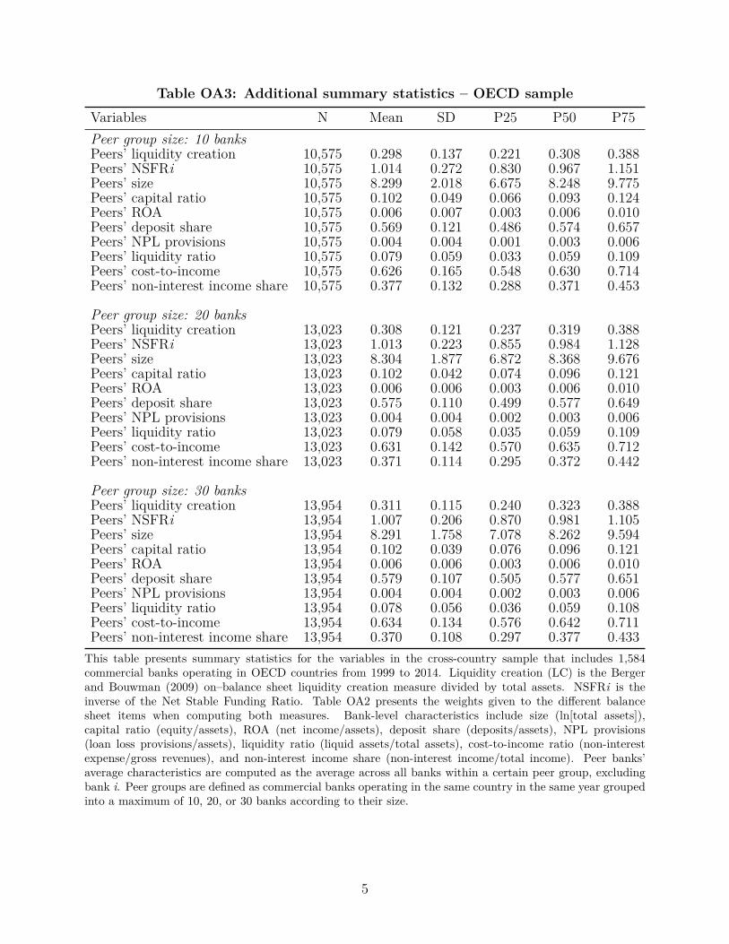
Table OA3: Additional summary statistics – OECD sampleVariables N Mean SD P25 P50 P75Peer group size: 10 banksPeers’ liquidity creation 10,575 0.298 0.137 0.221 0.308 0.388Peers’ NSFRi 10,575 1.014 0.272 0.830 0.967 1.151Peers’ size 10,575 8.299 2.018 6.675 8.248 9.775Peers’ capital ratio 10,575 0.102 0.049 0.066 0.093 0.124Peers’ ROA 10,575 0.006 0.007 0.003 0.006 0.010Peers’ deposit share 10,575 0.569 0.121 0.486 0.574 0.657Peers’ NPL provisions 10,575 0.004 0.004 0.001 0.003 0.006Peers’ liquidity ratio 10,575 0.079 0.059 0.033 0.059 0.109Peers’ cost-to-income 10,575 0.626 0.165 0.548 0.630 0.714Peers’ non-interest income share 10,575 0.377 0.132 0.288 0.371 0.453
Peer group size: 20 banksPeers’ liquidity creation 13,023 0.308 0.121 0.237 0.319 0.388Peers’ NSFRi 13,023 1.013 0.223 0.855 0.984 1.128Peers’ size 13,023 8.304 1.877 6.872 8.368 9.676Peers’ capital ratio 13,023 0.102 0.042 0.074 0.096 0.121Peers’ ROA 13,023 0.006 0.006 0.003 0.006 0.010Peers’ deposit share 13,023 0.575 0.110 0.499 0.577 0.649Peers’ NPL provisions 13,023 0.004 0.004 0.002 0.003 0.006Peers’ liquidity ratio 13,023 0.079 0.058 0.035 0.059 0.109Peers’ cost-to-income 13,023 0.631 0.142 0.570 0.635 0.712Peers’ non-interest income share 13,023 0.371 0.114 0.295 0.372 0.442
Peer group size: 30 banksPeers’ liquidity creation 13,954 0.311 0.115 0.240 0.323 0.388Peers’ NSFRi 13,954 1.007 0.206 0.870 0.981 1.105Peers’ size 13,954 8.291 1.758 7.078 8.262 9.594Peers’ capital ratio 13,954 0.102 0.039 0.076 0.096 0.121Peers’ ROA 13,954 0.006 0.006 0.003 0.006 0.010Peers’ deposit share 13,954 0.579 0.107 0.505 0.577 0.651Peers’ NPL provisions 13,954 0.004 0.004 0.002 0.003 0.006Peers’ liquidity ratio 13,954 0.078 0.056 0.036 0.059 0.108Peers’ cost-to-income 13,954 0.634 0.134 0.576 0.642 0.711Peers’ non-interest income share 13,954 0.370 0.108 0.297 0.377 0.433
This table presents summary statistics for the variables in the cross-country sample that includes 1,584commercial banks operating in OECD countries from 1999 to 2014. Liquidity creation (LC) is the Bergerand Bouwman (2009) on–balance sheet liquidity creation measure divided by total assets. NSFRi is theinverse of the Net Stable Funding Ratio. Table OA2 presents the weights given to the different balancesheet items when computing both measures. Bank-level characteristics include size (ln[total assets]),capital ratio (equity/assets), ROA (net income/assets), deposit share (deposits/assets), NPL provisions(loan loss provisions/assets), liquidity ratio (liquid assets/total assets), cost-to-income ratio (non-interestexpense/gross revenues), and non-interest income share (non-interest income/total income). Peer banks’average characteristics are computed as the average across all banks within a certain peer group, excludingbank i. Peer groups are defined as commercial banks operating in the same country in the same year groupedinto a maximum of 10, 20, or 30 banks according to their size.
5

Table OA4: Summary statistics – U.S. sampleVariables N Mean SD P25 P50 P75Liquidity mismatch indicators:Liquidity creation – on– and off–B/S 14,407 0.474 0.183 0.354 0.477 0.596Liquidity creation – on–B/S 14,407 0.367 0.150 0.277 0.375 0.469Liquidity creation – asset side 14,407 0.144 0.149 0.051 0.151 0.244Liquidity creation – liability side 14,407 0.224 0.085 0.167 0.222 0.282Liquidity creation – off–B/S 14,407 0.105 0.058 0.063 0.093 0.134LMIi – on– and off–B/S 9,960 -0.449 0.161 -0.549 -0.465 -0.360LMIi – on–B/S 9,960 -0.451 0.158 -0.549 -0.465 -0.362
Bank-level characteristics:Size 14,407 14.38 1.343 13.44 14.12 15.03Capital ratio 14,407 0.095 0.022 0.080 0.092 0.106ROA 14,407 0.005 0.008 0.002 0.005 0.009Deposit share 14,407 0.783 0.082 0.733 0.797 0.843NPL provisions 14,407 0.003 0.005 0.001 0.001 0.003
This table presents summary statistics for the main variables in the quarterly U.S. sample that includes 472listed commercial banks operating in the United States from 1999:Q1 to 2014:Q4. Liquidity creation (LC) isthe Berger and Bouwman (2009) on– and off–balance sheet and on–balance sheet liquidity creation measuresdivided by total assets. LMI is the Bai, Krishnamurthy, and Weymuller (2018) Liquidity Mismatch Index. Ireverse the signs of the LMI and express it as a share of total assets (LMIi) so that this measure is directlycomparable to the Berger and Bouwman (2009) indicator. Bank-level characteristics include size (ln[totalassets]), capital ratio (equity/assets), ROA (net income/assets), deposit share (deposits/assets), and NPLprovisions (loan loss provisions/assets).
6
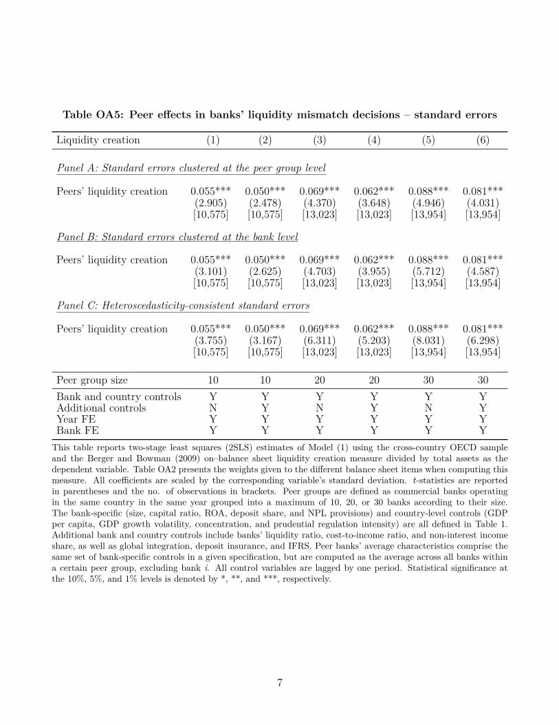
Table OA5: Peer effects in banks’ liquidity mismatch decisions – standard errors
Liquidity creation (1) (2) (3) (4) (5) (6)
Panel A: Standard errors clustered at the peer group level
Peers’ liquidity creation 0.055*** 0.050*** 0.069*** 0.062*** 0.088*** 0.081***(2.905) (2.478) (4.370) (3.648) (4.946) (4.031)[10,575] [10,575] [13,023] [13,023] [13,954] [13,954]
Panel B: Standard errors clustered at the bank level
Peers’ liquidity creation 0.055*** 0.050*** 0.069*** 0.062*** 0.088*** 0.081***(3.101) (2.625) (4.703) (3.955) (5.712) (4.587)[10,575] [10,575] [13,023] [13,023] [13,954] [13,954]
Panel C: Heteroscedasticity-consistent standard errors
Peers’ liquidity creation 0.055*** 0.050*** 0.069*** 0.062*** 0.088*** 0.081***(3.755) (3.167) (6.311) (5.203) (8.031) (6.298)[10,575] [10,575] [13,023] [13,023] [13,954] [13,954]
Peer group size 10 10 20 20 30 30Bank and country controls Y Y Y Y Y YAdditional controls N Y N Y N YYear FE Y Y Y Y Y YBank FE Y Y Y Y Y Y
This table reports two-stage least squares (2SLS) estimates of Model (1) using the cross-country OECD sampleand the Berger and Bowman (2009) on–balance sheet liquidity creation measure divided by total assets as thedependent variable. Table OA2 presents the weights given to the different balance sheet items when computing thismeasure. All coefficients are scaled by the corresponding variable’s standard deviation. t-statistics are reportedin parentheses and the no. of observations in brackets. Peer groups are defined as commercial banks operatingin the same country in the same year grouped into a maximum of 10, 20, or 30 banks according to their size.The bank-specific (size, capital ratio, ROA, deposit share, and NPL provisions) and country-level controls (GDPper capita, GDP growth volatility, concentration, and prudential regulation intensity) are all defined in Table 1.Additional bank and country controls include banks’ liquidity ratio, cost-to-income ratio, and non-interest incomeshare, as well as global integration, deposit insurance, and IFRS. Peer banks’ average characteristics comprise thesame set of bank-specific controls in a given specification, but are computed as the average across all banks withina certain peer group, excluding bank i. All control variables are lagged by one period. Statistical significance atthe 10%, 5%, and 1% levels is denoted by *, **, and ***, respectively.
7
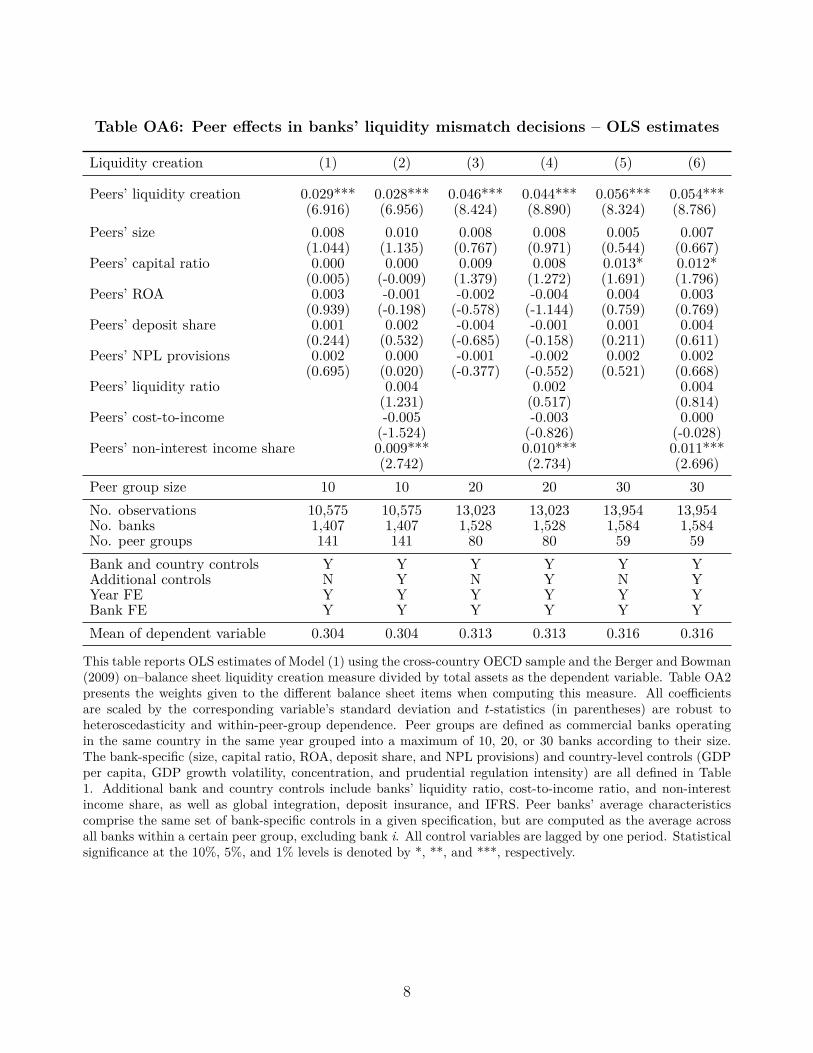
Table OA6: Peer effects in banks’ liquidity mismatch decisions – OLS estimates
Liquidity creation (1) (2) (3) (4) (5) (6)
Peers’ liquidity creation 0.029*** 0.028*** 0.046*** 0.044*** 0.056*** 0.054***(6.916) (6.956) (8.424) (8.890) (8.324) (8.786)
Peers’ size 0.008 0.010 0.008 0.008 0.005 0.007(1.044) (1.135) (0.767) (0.971) (0.544) (0.667)
Peers’ capital ratio 0.000 0.000 0.009 0.008 0.013* 0.012*(0.005) (-0.009) (1.379) (1.272) (1.691) (1.796)
Peers’ ROA 0.003 -0.001 -0.002 -0.004 0.004 0.003(0.939) (-0.198) (-0.578) (-1.144) (0.759) (0.769)
Peers’ deposit share 0.001 0.002 -0.004 -0.001 0.001 0.004(0.244) (0.532) (-0.685) (-0.158) (0.211) (0.611)
Peers’ NPL provisions 0.002 0.000 -0.001 -0.002 0.002 0.002(0.695) (0.020) (-0.377) (-0.552) (0.521) (0.668)
Peers’ liquidity ratio 0.004 0.002 0.004(1.231) (0.517) (0.814)
Peers’ cost-to-income -0.005 -0.003 0.000(-1.524) (-0.826) (-0.028)
Peers’ non-interest income share 0.009*** 0.010*** 0.011***(2.742) (2.734) (2.696)
Peer group size 10 10 20 20 30 30No. observations 10,575 10,575 13,023 13,023 13,954 13,954No. banks 1,407 1,407 1,528 1,528 1,584 1,584No. peer groups 141 141 80 80 59 59Bank and country controls Y Y Y Y Y YAdditional controls N Y N Y N YYear FE Y Y Y Y Y YBank FE Y Y Y Y Y YMean of dependent variable 0.304 0.304 0.313 0.313 0.316 0.316
This table reports OLS estimates of Model (1) using the cross-country OECD sample and the Berger and Bowman(2009) on–balance sheet liquidity creation measure divided by total assets as the dependent variable. Table OA2presents the weights given to the different balance sheet items when computing this measure. All coefficientsare scaled by the corresponding variable’s standard deviation and t-statistics (in parentheses) are robust toheteroscedasticity and within-peer-group dependence. Peer groups are defined as commercial banks operatingin the same country in the same year grouped into a maximum of 10, 20, or 30 banks according to their size.The bank-specific (size, capital ratio, ROA, deposit share, and NPL provisions) and country-level controls (GDPper capita, GDP growth volatility, concentration, and prudential regulation intensity) are all defined in Table1. Additional bank and country controls include banks’ liquidity ratio, cost-to-income ratio, and non-interestincome share, as well as global integration, deposit insurance, and IFRS. Peer banks’ average characteristicscomprise the same set of bank-specific controls in a given specification, but are computed as the average acrossall banks within a certain peer group, excluding bank i. All control variables are lagged by one period. Statisticalsignificance at the 10%, 5%, and 1% levels is denoted by *, **, and ***, respectively.
8
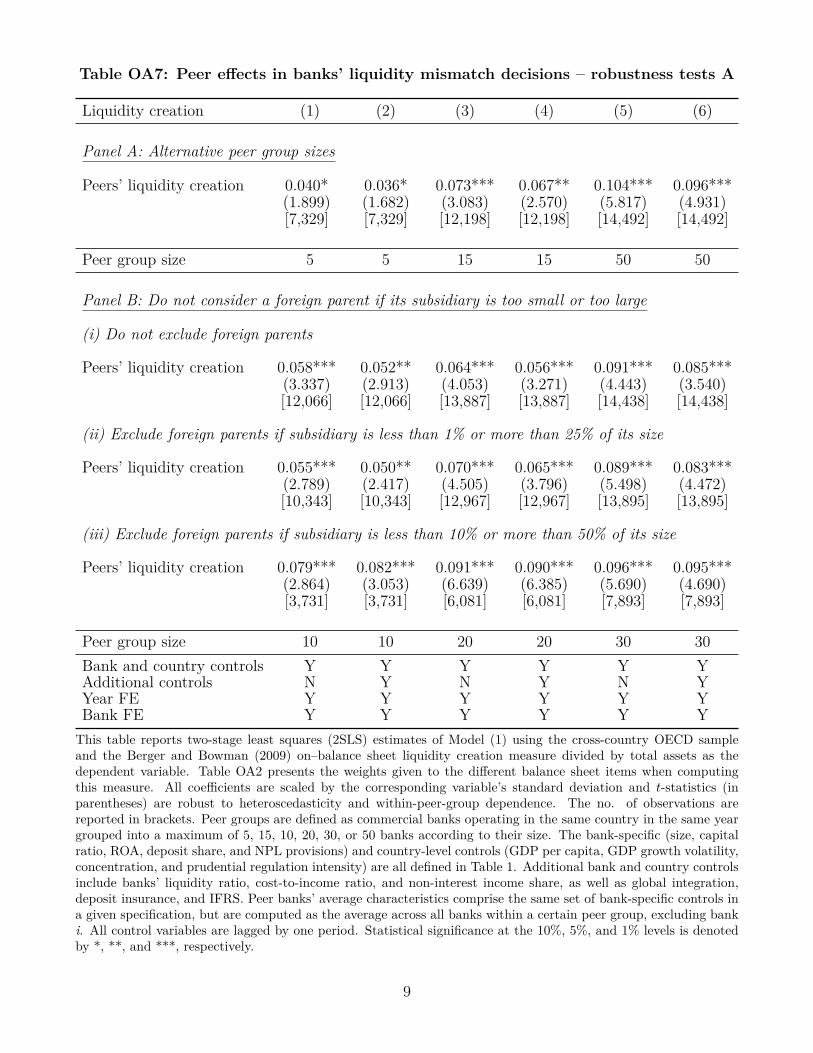
Table OA7: Peer effects in banks’ liquidity mismatch decisions – robustness tests A
Liquidity creation (1) (2) (3) (4) (5) (6)
Panel A: Alternative peer group sizes
Peers’ liquidity creation 0.040* 0.036* 0.073*** 0.067** 0.104*** 0.096***(1.899) (1.682) (3.083) (2.570) (5.817) (4.931)[7,329] [7,329] [12,198] [12,198] [14,492] [14,492]
Peer group size 5 5 15 15 50 50
Panel B: Do not consider a foreign parent if its subsidiary is too small or too large
(i) Do not exclude foreign parents
Peers’ liquidity creation 0.058*** 0.052** 0.064*** 0.056*** 0.091*** 0.085***(3.337) (2.913) (4.053) (3.271) (4.443) (3.540)[12,066] [12,066] [13,887] [13,887] [14,438] [14,438]
(ii) Exclude foreign parents if subsidiary is less than 1% or more than 25% of its size
Peers’ liquidity creation 0.055*** 0.050** 0.070*** 0.065*** 0.089*** 0.083***(2.789) (2.417) (4.505) (3.796) (5.498) (4.472)[10,343] [10,343] [12,967] [12,967] [13,895] [13,895]
(iii) Exclude foreign parents if subsidiary is less than 10% or more than 50% of its size
Peers’ liquidity creation 0.079*** 0.082*** 0.091*** 0.090*** 0.096*** 0.095***(2.864) (3.053) (6.639) (6.385) (5.690) (4.690)[3,731] [3,731] [6,081] [6,081] [7,893] [7,893]
Peer group size 10 10 20 20 30 30Bank and country controls Y Y Y Y Y YAdditional controls N Y N Y N YYear FE Y Y Y Y Y YBank FE Y Y Y Y Y Y
This table reports two-stage least squares (2SLS) estimates of Model (1) using the cross-country OECD sampleand the Berger and Bowman (2009) on–balance sheet liquidity creation measure divided by total assets as thedependent variable. Table OA2 presents the weights given to the different balance sheet items when computingthis measure. All coefficients are scaled by the corresponding variable’s standard deviation and t-statistics (inparentheses) are robust to heteroscedasticity and within-peer-group dependence. The no. of observations arereported in brackets. Peer groups are defined as commercial banks operating in the same country in the same yeargrouped into a maximum of 5, 15, 10, 20, 30, or 50 banks according to their size. The bank-specific (size, capitalratio, ROA, deposit share, and NPL provisions) and country-level controls (GDP per capita, GDP growth volatility,concentration, and prudential regulation intensity) are all defined in Table 1. Additional bank and country controlsinclude banks’ liquidity ratio, cost-to-income ratio, and non-interest income share, as well as global integration,deposit insurance, and IFRS. Peer banks’ average characteristics comprise the same set of bank-specific controls ina given specification, but are computed as the average across all banks within a certain peer group, excluding banki. All control variables are lagged by one period. Statistical significance at the 10%, 5%, and 1% levels is denotedby *, **, and ***, respectively.
9
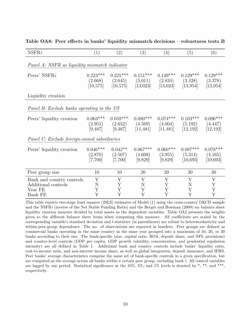
Table OA8: Peer effects in banks’ liquidity mismatch decisions – robustness tests B
NSFRi (1) (2) (3) (4) (5) (6)
Panel A: NSFR as liquidity mismatch indicator
Peers’ NSFRi 0.223*** 0.225*** 0.151*** 0.149*** 0.129*** 0.129***(2.668) (2.645) (3.011) (2.834) (3.428) (3.378)[10,575] [10,575] [13,023] [13,023] [13,954] [13,954]
Liquidity creation
Panel B: Exclude banks operating in the US
Peers’ liquidity creation 0.063*** 0.059*** 0.080*** 0.074*** 0.103*** 0.096***(2.951) (2.652) (4.569) (4.004) (5.192) (4.447)[9,487] [9,487] [11,481] [11,481] [12,192] [12,192]
Panel C: Exclude foreign-owned subsidiaries
Peers’ liquidity creation 0.046*** 0.042** 0.067*** 0.060*** 0.087*** 0.078***(2.870) (2.507) (4.608) (3.955) (5.314) (4.165)[7,700] [7,700] [9,829] [9,829] [10,693] [10,693]
Peer group size 10 10 20 20 30 30Bank and country controls Y Y Y Y Y YAdditional controls N Y N Y N YYear FE Y Y Y Y Y YBank FE Y Y Y Y Y Y
This table reports two-stage least squares (2SLS) estimates of Model (1) using the cross-country OECD sampleand the NSFRi (inverse of the Net Stable Funding Ratio) and the Berger and Bowman (2009) on–balance sheetliquidity creation measure divided by total assets as the dependent variables. Table OA2 presents the weightsgiven to the different balance sheet items when computing this measure. All coefficients are scaled by thecorresponding variable’s standard deviation and t-statistics (in parentheses) are robust to heteroscedasticity andwithin-peer-group dependence. The no. of observations are reported in brackets. Peer groups are defined ascommercial banks operating in the same country in the same year grouped into a maximum of 10, 20, or 30banks according to their size. The bank-specific (size, capital ratio, ROA, deposit share, and NPL provisions)and country-level controls (GDP per capita, GDP growth volatility, concentration, and prudential regulationintensity) are all defined in Table 1. Additional bank and country controls include banks’ liquidity ratio,cost-to-income ratio, and non-interest income share, as well as global integration, deposit insurance, and IFRS.Peer banks’ average characteristics comprise the same set of bank-specific controls in a given specification, butare computed as the average across all banks within a certain peer group, excluding bank i. All control variablesare lagged by one period. Statistical significance at the 10%, 5%, and 1% levels is denoted by *, **, and ***,respectively.
10

Table OA9: Peer effects in banks’ liquidity mismatch decisions – robustness tests C
Liquidity creation (1) (2) (3) (4) (5) (6)
Panel A: Lagged peers banks’ liquidity creation
Peers’ liquidity creation 0.061*** 0.058** 0.074*** 0.067*** 0.098*** 0.094***(2.895) (2.568) (3.997) (3.212) (6.283) (5.690)[10,371] [10,371] [12,873] [12,873] [13,876] [13,876]
Panel B: No winsorizing of control variables
Peers’ liquidity creation 0.056*** 0.052** 0.070*** 0.064*** 0.089*** 0.082***(2.956) (2.529) (4.474) (3.745) (5.017) (4.082)[10,575] [10,575] [13,023] [13,023] [13,954] [13,954]
Panel C: Drop banks with asset growth above 75% in any of the years
Peers’ liquidity creation 0.065*** 0.059*** 0.065*** 0.058*** 0.075*** 0.065***(3.054) (2.622) (4.088) (3.338) (3.980) (3.004)[8,169] [8,169] [10,043] [10,043] [10,767] [10,767]
Peer group size 10 10 20 20 30 30Bank and country controls Y Y Y Y Y YAdditional controls N Y N Y N YYear FE Y Y Y Y Y YBank FE Y Y Y Y Y Y
This table reports two-stage least squares (2SLS) estimates of Model (1) using the cross-country OECD sampleand the Berger and Bowman (2009) on–balance sheet liquidity creation measure divided by total assets as thedependent variable. Table OA2 presents the weights given to the different balance sheet items when computingthis measure. All coefficients are scaled by the corresponding variable’s standard deviation and t-statistics (inparentheses) are robust to heteroscedasticity and within-peer-group dependence. The no. of observations arereported in brackets. Peer groups are defined as commercial banks operating in the same country in the sameyear grouped into a maximum of 10, 20, or 30 banks according to their size. The bank-specific (size, capital ratio,ROA, deposit share, and NPL provisions) and country-level controls (GDP per capita, GDP growth volatility,concentration, and prudential regulation intensity) are all defined in Table 1. Additional bank and country controlsinclude banks’ liquidity ratio, cost-to-income ratio, and non-interest income share, as well as global integration,deposit insurance, and IFRS. Peer banks’ average characteristics comprise the same set of bank-specific controls ina given specification, but are computed as the average across all banks within a certain peer group, excluding banki. All control variables are lagged by one period. Statistical significance at the 10%, 5%, and 1% levels is denotedby *, **, and ***, respectively.
11
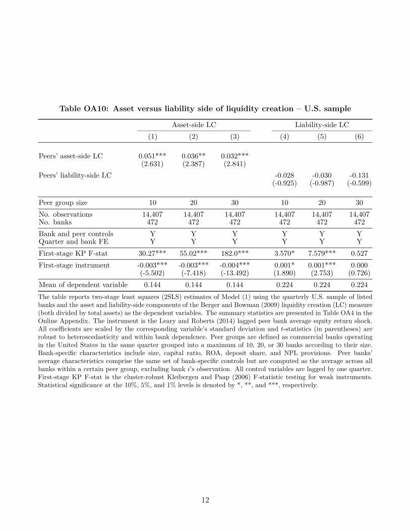
Table OA10: Asset versus liability side of liquidity creation – U.S. sample
Asset-side LC Liability-side LC(1) (2) (3) (4) (5) (6)
Peers’ asset-side LC 0.051*** 0.036** 0.032***(2.631) (2.387) (2.841)
Peers’ liability-side LC -0.028 -0.030 -0.131(-0.925) (-0.987) (-0.599)
Peer group size 10 20 30 10 20 30No. observations 14,407 14,407 14,407 14,407 14,407 14,407No. banks 472 472 472 472 472 472Bank and peer controls Y Y Y Y Y YQuarter and bank FE Y Y Y Y Y YFirst-stage KP F-stat 30.27*** 55.02*** 182.0*** 3.570* 7.579*** 0.527First-stage instrument -0.003*** -0.003*** -0.004*** 0.001* 0.001*** 0.000
(-5.502) (-7.418) (-13.492) (1.890) (2.753) (0.726)Mean of dependent variable 0.144 0.144 0.144 0.224 0.224 0.224The table reports two-stage least squares (2SLS) estimates of Model (1) using the quarterly U.S. sample of listedbanks and the asset and liability-side components of the Berger and Bowman (2009) liquidity creation (LC) measure(both divided by total assets) as the dependent variables. The summary statistics are presented in Table OA4 in theOnline Appendix. The instrument is the Leary and Roberts (2014) lagged peer bank average equity return shock.All coefficients are scaled by the corresponding variable’s standard deviation and t-statistics (in parentheses) arerobust to heteroscedasticity and within bank dependence. Peer groups are defined as commercial banks operatingin the United States in the same quarter grouped into a maximum of 10, 20, or 30 banks according to their size.Bank-specific characteristics include size, capital ratio, ROA, deposit share, and NPL provisions. Peer banks’average characteristics comprise the same set of bank-specific controls but are computed as the average across allbanks within a certain peer group, excluding bank i’s observation. All control variables are lagged by one quarter.First-stage KP F-stat is the cluster-robust Kleibergen and Paap (2006) F-statistic testing for weak instruments.Statistical significance at the 10%, 5%, and 1% levels is denoted by *, **, and ***, respectively.
12
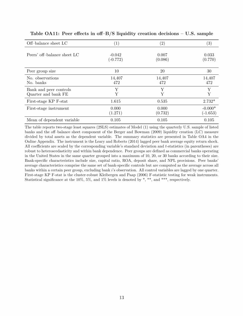
Table OA11: Peer effects in off–B/S liquidity creation decisions – U.S. sample
Off–balance sheet LC (1) (2) (3)
Peers’ off–balance sheet LC -0.042 0.007 0.033(-0.772) (0.086) (0.770)
Peer group size 10 20 30No. observations 14,407 14,407 14,407No. banks 472 472 472Bank and peer controls Y Y YQuarter and bank FE Y Y YFirst-stage KP F-stat 1.615 0.535 2.732*First-stage instrument 0.000 0.000 -0.000*
(1.271) (0.732) (-1.653)Mean of dependent variable 0.105 0.105 0.105
The table reports two-stage least squares (2SLS) estimates of Model (1) using the quarterly U.S. sample of listedbanks and the off–balance sheet component of the Berger and Bowman (2009) liquidity creation (LC) measuredivided by total assets as the dependent variable. The summary statistics are presented in Table OA4 in theOnline Appendix. The instrument is the Leary and Roberts (2014) lagged peer bank average equity return shock.All coefficients are scaled by the corresponding variable’s standard deviation and t-statistics (in parentheses) arerobust to heteroscedasticity and within bank dependence. Peer groups are defined as commercial banks operatingin the United States in the same quarter grouped into a maximum of 10, 20, or 30 banks according to their size.Bank-specific characteristics include size, capital ratio, ROA, deposit share, and NPL provisions. Peer banks’average characteristics comprise the same set of bank-specific controls but are computed as the average across allbanks within a certain peer group, excluding bank i’s observation. All control variables are lagged by one quarter.First-stage KP F-stat is the cluster-robust Kleibergen and Paap (2006) F-statistic testing for weak instruments.Statistical significance at the 10%, 5%, and 1% levels is denoted by *, **, and ***, respectively.
13
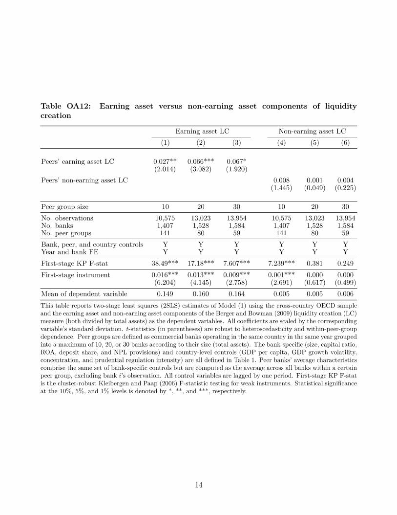
Table OA12: Earning asset versus non-earning asset components of liquiditycreation
Earning asset LC Non-earning asset LC(1) (2) (3) (4) (5) (6)
Peers’ earning asset LC 0.027** 0.066*** 0.067*(2.014) (3.082) (1.920)
Peers’ non-earning asset LC 0.008 0.001 0.004(1.445) (0.049) (0.225)
Peer group size 10 20 30 10 20 30No. observations 10,575 13,023 13,954 10,575 13,023 13,954No. banks 1,407 1,528 1,584 1,407 1,528 1,584No. peer groups 141 80 59 141 80 59Bank, peer, and country controls Y Y Y Y Y YYear and bank FE Y Y Y Y Y YFirst-stage KP F-stat 38.49*** 17.18*** 7.607*** 7.239*** 0.381 0.249First-stage instrument 0.016*** 0.013*** 0.009*** 0.001*** 0.000 0.000
(6.204) (4.145) (2.758) (2.691) (0.617) (0.499)Mean of dependent variable 0.149 0.160 0.164 0.005 0.005 0.006This table reports two-stage least squares (2SLS) estimates of Model (1) using the cross-country OECD sampleand the earning asset and non-earning asset components of the Berger and Bowman (2009) liquidity creation (LC)measure (both divided by total assets) as the dependent variables. All coefficients are scaled by the correspondingvariable’s standard deviation. t-statistics (in parentheses) are robust to heteroscedasticity and within-peer-groupdependence. Peer groups are defined as commercial banks operating in the same country in the same year groupedinto a maximum of 10, 20, or 30 banks according to their size (total assets). The bank-specific (size, capital ratio,ROA, deposit share, and NPL provisions) and country-level controls (GDP per capita, GDP growth volatility,concentration, and prudential regulation intensity) are all defined in Table 1. Peer banks’ average characteristicscomprise the same set of bank-specific controls but are computed as the average across all banks within a certainpeer group, excluding bank i’s observation. All control variables are lagged by one period. First-stage KP F-statis the cluster-robust Kleibergen and Paap (2006) F-statistic testing for weak instruments. Statistical significanceat the 10%, 5%, and 1% levels is denoted by *, **, and ***, respectively.
14
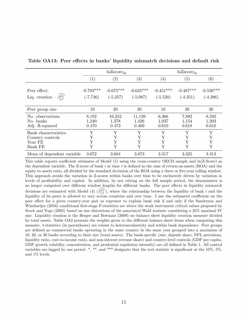
Table OA13: Peer effects in banks’ liquidity mismatch decisions and default risk
lnZscore3y lnZscore5y
(1) (2) (3) (4) (5) (6)
Peer effect: -0.793*** -0.675*** -0.635*** -0.451*** -0.487*** -0.526***Liq. creation – βLC
j,t (-7.746) (-5.257) (-5.087) (-5.520) (-4.351) (-4.386)
Peer group size 10 20 30 10 20 30No. observations 8,192 10,352 11,139 6,366 7,892 8,592No. banks 1,240 1,378 1,426 1,037 1,154 1,203Adj. R-squared 0.470 0.473 0.469 0.610 0.618 0.610Bank characteristics Y Y Y Y Y YCountry controls Y Y Y Y Y YYear FE Y Y Y Y Y YBank FE Y Y Y Y Y YMean of dependent variable 3.672 3.684 3.673 3.317 3.325 3.313
This table reports coefficient estimates of Model (5) using the cross-country OECD sample and ln(Z-Score) asthe dependent variable. The Z-score of bank i at time t is defined as the sum of return-on-assets (ROA) and theequity to assets ratio, all divided by the standard deviation of the ROA using a three or five-year rolling window.This approach avoids the variation in Z-scores within banks over time to be exclusively driven by variation inlevels of profitability and capital. In addition, by not relying on the full sample period, the denominator isno longer computed over different window lengths for different banks. The peer effects in liquidity mismatchdecisions are estimated with Model (4) (βLC
j,t ), where the relationship between the liquidity of bank i and theliquidity of its peers is allowed to vary across countries and over time. I use the estimated coefficient on thepeer effect for a given country-year pair as regressor to explain bank risk if and only if the Sanderson andWindmeijer (2016) conditional first-stage F-statistics are above the weak instrument critical values proposed byStock and Yogo (2005) based on size distortions of the associated Wald statistic considering a 25% maximal IVsize. Liquidity creation is the Berger and Bowman (2009) on–balance sheet liquidity creation measure dividedby total assets. Table OA2 presents the weights given to the different balance sheet items when computing thismeasure. t-statistics (in parentheses) are robust to heteroscedasticity and within bank dependence. Peer groupsare defined as commercial banks operating in the same country in the same year grouped into a maximum of10, 20, or 30 banks according to their size (total assets). The bank-specific (size, deposit share, NPL provisions,liquidity ratio, cost-to-income ratio, and non-interest revenue share) and country-level controls (GDP per capita,GDP growth volatility, concentration, and prudential regulation intensity) are all defined in Table 1. All controlvariables are lagged by one period. *, **, and *** designate that the test statistic is significant at the 10%, 5%,and 1% levels.
15
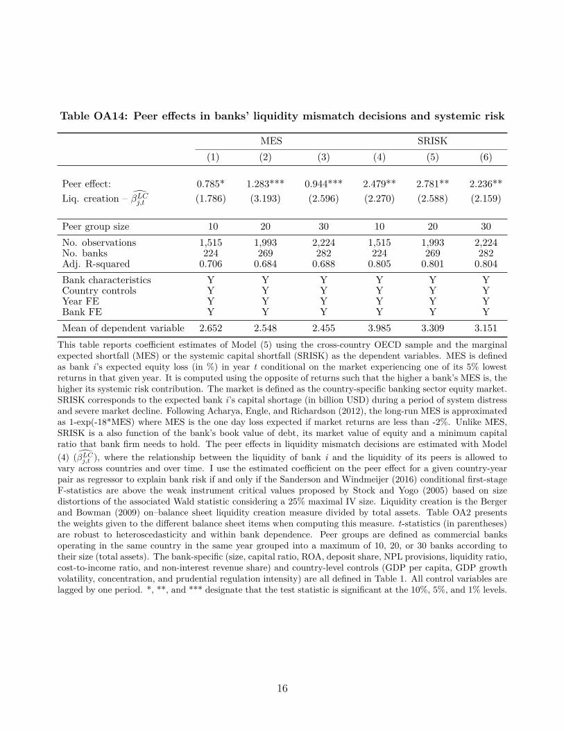
Table OA14: Peer effects in banks’ liquidity mismatch decisions and systemic risk
MES SRISK(1) (2) (3) (4) (5) (6)
Peer effect: 0.785* 1.283*** 0.944*** 2.479** 2.781** 2.236**Liq. creation – βLC
j,t (1.786) (3.193) (2.596) (2.270) (2.588) (2.159)
Peer group size 10 20 30 10 20 30No. observations 1,515 1,993 2,224 1,515 1,993 2,224No. banks 224 269 282 224 269 282Adj. R-squared 0.706 0.684 0.688 0.805 0.801 0.804Bank characteristics Y Y Y Y Y YCountry controls Y Y Y Y Y YYear FE Y Y Y Y Y YBank FE Y Y Y Y Y YMean of dependent variable 2.652 2.548 2.455 3.985 3.309 3.151
This table reports coefficient estimates of Model (5) using the cross-country OECD sample and the marginalexpected shortfall (MES) or the systemic capital shortfall (SRISK) as the dependent variables. MES is definedas bank i’s expected equity loss (in %) in year t conditional on the market experiencing one of its 5% lowestreturns in that given year. It is computed using the opposite of returns such that the higher a bank’s MES is, thehigher its systemic risk contribution. The market is defined as the country-specific banking sector equity market.SRISK corresponds to the expected bank i’s capital shortage (in billion USD) during a period of system distressand severe market decline. Following Acharya, Engle, and Richardson (2012), the long-run MES is approximatedas 1-exp(-18*MES) where MES is the one day loss expected if market returns are less than -2%. Unlike MES,SRISK is a also function of the bank’s book value of debt, its market value of equity and a minimum capitalratio that bank firm needs to hold. The peer effects in liquidity mismatch decisions are estimated with Model(4) (βLC
j,t ), where the relationship between the liquidity of bank i and the liquidity of its peers is allowed tovary across countries and over time. I use the estimated coefficient on the peer effect for a given country-yearpair as regressor to explain bank risk if and only if the Sanderson and Windmeijer (2016) conditional first-stageF-statistics are above the weak instrument critical values proposed by Stock and Yogo (2005) based on sizedistortions of the associated Wald statistic considering a 25% maximal IV size. Liquidity creation is the Bergerand Bowman (2009) on–balance sheet liquidity creation measure divided by total assets. Table OA2 presentsthe weights given to the different balance sheet items when computing this measure. t-statistics (in parentheses)are robust to heteroscedasticity and within bank dependence. Peer groups are defined as commercial banksoperating in the same country in the same year grouped into a maximum of 10, 20, or 30 banks according totheir size (total assets). The bank-specific (size, capital ratio, ROA, deposit share, NPL provisions, liquidity ratio,cost-to-income ratio, and non-interest revenue share) and country-level controls (GDP per capita, GDP growthvolatility, concentration, and prudential regulation intensity) are all defined in Table 1. All control variables arelagged by one period. *, **, and *** designate that the test statistic is significant at the 10%, 5%, and 1% levels.
16