Stimulus-Specific Adaptation in the Auditory Thalamusof the Anesthetized RatFlora M. Antunes1, Israel Nelken3,4, Ellen Covey5, Manuel S. Malmierca1,2*
1 Auditory Neurophysiology Unit, Laboratory for the Neurobiology of Hearing, Institute of Neuroscience of Castilla y Leon, University of Salamanca, Salamanca, Spain,
2 Department of Cell Biology and Pathology, Faculty of Medicine, University of Salamanca, Salamanca, Spain, 3 Department of Neurobiology, Institute of Life Sciences, The
Hebrew University of Jerusalem, Jerusalem, Israel, 4 The Edmond and Lily Safra Center for Brain Sciences, The Hebrew University of Jerusalem, Jerusalem, Israel,
5 Department of Psychology, University of Washington, Seattle, Washington, United States of America
Abstract
The specific adaptation of neuronal responses to a repeated stimulus (Stimulus-specific adaptation, SSA), which does notfully generalize to other stimuli, provides a mechanism for emphasizing rare and potentially interesting sensory events.Previous studies have demonstrated that neurons in the auditory cortex and inferior colliculus show SSA. However, thecontribution of the medial geniculate body (MGB) and its main subdivisions to SSA and detection of rare sounds remainspoorly characterized. We recorded from single neurons in the MGB of anaesthetized rats while presenting a sequencecomposed of a rare tone presented in the context of a common tone (oddball sequences). We demonstrate that asignificant percentage of neurons in MGB adapt in a stimulus-specific manner. Neurons in the medial and dorsalsubdivisions showed the strongest SSA, linking this property to the non-lemniscal pathway. Some neurons in the non-lemniscal regions showed strong SSA even under extreme testing conditions (e.g., a frequency interval of 0.14 octavescombined with a stimulus onset asynchrony of 2000 ms). Some of these neurons were able to discriminate between twovery close frequencies (frequency interval of 0.057 octaves), revealing evidence of hyperacuity in neurons at a subcorticallevel. Thus, SSA is expressed strongly in the rat auditory thalamus and contribute significantly to auditory change detection.
Citation: Antunes FM, Nelken I, Covey E, Malmierca MS (2010) Stimulus-Specific Adaptation in the Auditory Thalamus of the Anesthetized Rat. PLoS ONE 5(11):e14071. doi:10.1371/journal.pone.0014071
Editor: Jun Yan, Hotchkiss Brain Institute, University of Calgary, Canada
Received July 30, 2010; Accepted October 29, 2010; Published November 19, 2010
Copyright: � 2010 Antunes et al. This is an open-access article distributed under the terms of the Creative Commons Attribution License, which permitsunrestricted use, distribution, and reproduction in any medium, provided the original author and source are credited.
Funding: Financial support was provided by the Spanish MEC (BFU2009-07286), EU (EUI2009-04083) and JCYL-UE (GR221) to MSM, the EU (EUI2009-04083) andthe Israeli Science Foundation (ISF) to IN and the NSF (IOS-0719295) to EC. Support for software development was provided by NIH (NIDCD P30DC004661); FMAheld a fellowship from the Spanish MEC (BES-2007-15642). The funders had no role in study design, data collection and analysis, decision to publish, orpreparation of the manuscript.
Competing Interests: The authors have declared that no competing interests exist.
* E-mail: [email protected]
Introduction
Rare sounds may indicate events of behavioural importance to
which an individual should attend for survival. On the other hand,
repeating sounds without behavioural consequences can be assumed
to be unimportant. Indeed, neurons at several levels of the auditory
system have been shown to signal the occurrence of rare sounds
while reducing their responses to repeated ones. The specific
adaptation to repeated sounds, which does not generalize to other
sounds, is referred to as stimulus-specific adaptation (SSA). Recent
SSA studies [1–13] have revealed that SSA in single auditory
neurons shares many similarities with Mismatch Negativity (MMN)
[5,14–18], and may contribute to auditory scene analysis [19].
The medial geniculate body (MGB) is the principal nucleus of
the auditory thalamus and possesses three main subdivisions:
ventral (MGV), dorsal (MGD) and medial (MGM) [20–22]. The
non-lemniscal divisions are morphologically and functionally
different from the lemniscal MGV [21,23–25]. The MGV
constitutes the lemniscal part of the auditory thalamus and is
thought to process basic acoustic features of the stimulus, whereas
the MGD and MGM comprise the non-lemniscal part, and are
thought to process more complex features.
The MGB receives ascending inputs from the inferior colliculus
(IC) [21,26,27] and massive descending inputs from the auditory
cortex (AC; [21,28–32]. SSA is known to be present in the
thalamus: Yu and colleagues [13] demonstrated strong SSA in the
reticular nucleus. However, a previous report of SSA in the MGB
of mice [1] showed substantially weaker levels of adaptation than
those found in AC [10–12] or IC [4] neurons. Given its
connections with the AC and the IC, one would expect neurons
in the MGB to show strong SSA as well. In particular, the
differences in the SSA exhibited by neurons in the three main
subdivisions of the MGB need to be clarified. The mouse MGB
study [1] showed SSA in the MGM and in the lemniscal MGV but
not in the non-lemniscal MGD subdivision. Nevertheless, the
studies of the rat IC [4,6] demonstrated stronger SSA in the non-
lemniscal regions than in the lemniscal central nucleus.
Here, using the same oddball paradigm as previously used in
AC and IC studies, we recorded from single neurons throughout
the rat MGB. We aimed to characterize SSA in its main
subdivisions under several conditions hitherto unexplored. Our
results demonstrate that MGB neurons exhibit SSA levels as high
as those found in the IC and AC. Furthermore, SSA is more
prominent in the medial and dorsal subdivisions, linking this
property to the non-lemniscal auditory pathway. Thus, we
demonstrate that the MGB has substantial SSA and strongly
represents frequency change detection. Preliminary results have
been presented elsewhere [33–35].
PLoS ONE | www.plosone.org 1 November 2010 | Volume 5 | Issue 11 | e14071
Results
To look for evidence of SSA in the MGB we recorded the
responses of single neurons (n = 93) while presenting sequences of
tones with two different frequencies (f1 and f2; 400 stimulus
presentations) in which the standard and deviant stimuli occurred
at different probability ratios (90/10% or 70/30%), with different
frequency intervals (Df = 0.37, 0.10 or 0.04) and at different
repetition rates (SOA = 2000 ms, 500 ms, 250 ms or 125 ms). We
localized 60 of the 93 units recorded to one of the three main
MGB subdivisions: 24 units were localized to the MGD; 18 to the
MGM; and 18 to the MGV. The remaining units could not be
localized with confidence and included units close to the borders
between subdivisions (15 out of 33).
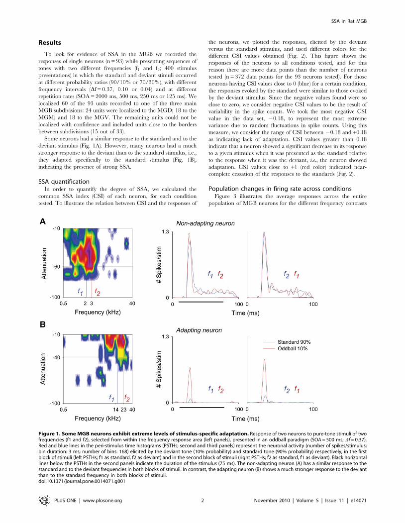
Some neurons had a similar response to the standard and to the
deviant stimulus (Fig. 1A). However, many neurons had a much
stronger response to the deviant than to the standard stimulus, i.e.,
they adapted specifically to the standard stimulus (Fig. 1B),
indicating the presence of strong SSA.
SSA quantificationIn order to quantify the degree of SSA, we calculated the
common SSA index (CSI) of each neuron, for each condition
tested. To illustrate the relation between CSI and the responses of
the neurons, we plotted the responses, elicited by the deviant
versus the standard stimulus, and used different colors for the
different CSI values obtained (Fig. 2). This figure shows the
responses of the neurons to all conditions tested, and for this
reason there are more data points than the number of neurons
tested (n = 372 data points for the 93 neurons tested). For those
neurons having CSI values close to 0 (blue) for a certain condition,
the responses evoked by the standard were similar to those evoked
by the deviant stimulus. Since the negative values found were so
close to zero, we consider negative CSI values to be the result of
variability in the spike counts. We took the most negative CSI
value in the data set, 20.18, to represent the most extreme
variance due to random fluctuations in spike counts. Using this
measure, we consider the range of CSI between 20.18 and +0.18
as indicating lack of adaptation. CSI values greater than 0.18
indicate that a neuron showed a significant decrease in its response
to a given stimulus when it was presented as the standard relative
to the response when it was the deviant, i.e., the neuron showed
adaptation. CSI values close to +1 (red color) indicated near-
complete cessation of the responses to the standards (Fig. 2).
Population changes in firing rate across conditionsFigure 3 illustrates the average responses across the entire
population of MGB neurons for the different frequency contrasts
Figure 1. Some MGB neurons exhibit extreme levels of stimulus-specific adaptation. Response of two neurons to pure-tone stimuli of twofrequencies (f1 and f2), selected from within the frequency response area (left panels), presented in an oddball paradigm (SOA = 500 ms; Df = 0.37).Red and blue lines in the peri-stimulus time histograms (PSTHs; second and third panels) represent the neuronal activity (number of spikes/stimulus;bin duration: 3 ms; number of bins: 168) elicited by the deviant tone (10% probability) and standard tone (90% probability) respectively, in the firstblock of stimuli (left PSTHs; f1 as standard, f2 as deviant) and in the second block of stimuli (right PSTHs; f2 as standard, f1 as deviant). Black horizontallines below the PSTHs in the second panels indicate the duration of the stimulus (75 ms). The non-adapting neuron (A) has a similar response to thestandard and to the deviant frequencies in both blocks of stimuli. In contrast, the adapting neuron (B) shows a much stronger response to the deviantthan to the standard frequency in both blocks of stimuli.doi:10.1371/journal.pone.0014071.g001
SSA in Rat MGB
PLoS ONE | www.plosone.org 2 November 2010 | Volume 5 | Issue 11 | e14071

and SOAs (repetition rates) tested at the highest standard-to-
deviant probability ratio (90/10%). Each plot shows the mean
peristimulus time histograms of the entire population, for each
combination of conditions (Fig. 3; red, deviant; blue, standard).
On average, the firing rate decreased as SOA decreased, i.e., firing
rate was highest at low stimulus repetition rates. This effect
presumably represents a form of non-specific adaptation, which
affects the responses to both standard and deviant stimuli.
The mean firing rate in response to the deviant was significantly
higher than that to the standard under all conditions, except when
Df was 0.04 (with a small effect for SOA = 250 ms; i.e., at a
repetition rate of 4/s, even at this small Df). However, a population
analysis of this type is biased disproportionately by neurons with
high firing rates. Since the neurons with the largest responses
tended to be non-adapting (e.g., compare neurons in Fig. 1A and
B, tested for the same conditions; see Fig. 2 for population
analysis), the responses of the highly-adapting neurons with lower
firing rates are downplayed in Fig. 3.
The data collected at the shortest SOA tested (125 ms) required
special treatment, since those neurons that exhibited the highest
levels of SSA at higher repetition rates (SOA = 250 and/or 500 ms
[4/s or 2/s]) were also those that had the largest overall reduction
in their firing at high repetition rates. In the extreme case, many
units (27/47) that exhibited high levels of SSA for an SOA of
250 ms completely ceased firing at the shortest SOA (125 ms) and
were not included in the analysis for this condition. The remaining
units (20/47) maintained some firing when tested at the 125 ms
SOA condition, resulting in high CSI values for all these
conditions. Figure 4 displays the responses of one of these high-
SSA neurons, localized in the MGM subdivision. This neuron
reduced substantially its responses for SOA = 125 ms, although its
responses were not completely abolished.
General description of SSA across the MGB populationTo analyze SSA across the population of MGB neurons, we
plotted the frequency-specific SSA index (SI) for the different
conditions separately, and used a different color to identify the
neurons that were located in the different subdivisions of MGB
(Fig. 5; Red, MGM; Orange, MGD; Blue, MGV; and Gray, non-
localized units).
For the majority of conditions, the plots show SI(fi) values
located above the reverse diagonal, which indicates the presence of
SSA [10]. The SI values for each frequency pair [SI(f1) and SI(f2)]
were very similar, leading to a distribution around the diagonal in
the upper right quadrant of the plot for most of the values (Fig. 5);
this demonstrates that the response did not depend on the
frequencies presented, but reflected genuine adaptation elicited by
the standard-deviant combination.
Across the entire population, the highest SSA values were found
for the largest Dfs (0.37 and 0.10) at intermediate SOAs (250 and
500 ms) and the lowest deviant probability (90/10%) conditions
(Fig. 5). The plots for these conditions show a cluster of points in
the upper right corner (Fig. 5); these points correspond to neurons
with an SI(fi).0.6 for both f1 and f2, which represent the highest
degree of selectivity to the rare tone. Under these conditions, a
high percentage of neurons showed CSI values in the range from
0.6 to 0.99, revealing strong SSA (56% and 27% at SOA = 500,
for Df = 0.37 and 0.10, respectively; 46% at SOA = 250 ms for
both Dfs; Fig. 5). Figures 4 and 6 show two examples of the
responses of such neurons, localized to the MGM and MGD,
respectively (For the units in Figs. 4 and 6, CSI.0.82 when
Figure 2. Responses of MGB neurons to the deviant andstandard tones across the CSI range. Scatterplot of the response ofall neurons to the deviant tone vs response to the standard tone, withpoints color-coded according to the CSI value (different colors, rightcolor bar). Low CSI values (around 0) correspond to neurons having asimilar response to the standard and deviant stimuli, i.e., non-adaptingneurons. Higher CSI values reflect a stronger response to the deviantthan to the standard stimulus, i.e., adaptation to the standard. CSIvalues close to +1 (red color) indicate near-complete cessation of theresponses to the standard tone. The most strongly responding neuronstended to be non-adapting.doi:10.1371/journal.pone.0014071.g002
Figure 3. Responses of the population of MGB neurons acrossstimulation conditions. Averaged post-stimulus time histograms (Binduration: 3 ms) for the entire population of MGB neurons across thedifferent conditions tested (Df and SOA) for the 90/10% probabilitycondition. The mean firing rate elicited by both stimuli (standard, bluelines; deviant, red lines) decreased directly with SOA (SOA = 2000, 500,250 and 125 ms; from first to fourth rows, respectively), for the differentDfs tested (Df = 0.37, 0.10 and 0.04; from first to third columns,respectively). Numbers in each plot indicate the number of neurons foreach condition. Black horizontal lines under the PSTHs of the bottomrow indicate the duration of the stimulus (75 ms).doi:10.1371/journal.pone.0014071.g003
SSA in Rat MGB
PLoS ONE | www.plosone.org 3 November 2010 | Volume 5 | Issue 11 | e14071

Df$0.1 and SOA = 250 or 500 ms). At the shortest SOA (125 ms),
some neurons failed to respond at all and for this reason fewer
neurons are represented in these plots (Fig. 5). Even so, some
neurons maintained a high degree of SSA under this condition
(Fig. 4, first row; Df = 0.1 and SOA = 125; CSI = 0.93).
Although the amount of SSA was reduced for the largest SOA
(2000 ms) and the smallest Df (0.04), we recorded neurons that
exhibited robust SSA under each of these conditions (Fig. 5).
Figure 4 shows the responses of a neuron that had a reduced, but
still high degree of adaptation at an SOA of 2000 ms (fourth row:
Df = 0.10, CSI = 0.40; compared to CSI.0.9 for shorter SOAs).
Other neurons had CSI.0.6 at SOAs of 2000 ms. For the smallest
Df (0.04) some neurons had CSI.0.6 as well (for SOA = 250 ms
and 500 ms, respectively; Fig. 5). Figure 6 shows an example of a
neuron that had a reduced, but still high degree of adaptation with
Df = 0.04 (SOA = 250 ms, CSI = 0.58). However, no neurons
showed SSA when tested with the combination of Df = 0.04 and
SOA = 2000 ms. This was in fact the only combination out of the
15 tested that did not elicit any SSA in the MGB population
(Fig. 5).
The amount of SSA was lower for the 70/30% condition;
although some neurons exhibited high SI values under this
Figure 4. Firing rate decreases as repetition rate increases in the MGB neurons. Example of an MGM neuron showing strong SSA acrossdifferent SOAs (125, 250, 500 and 2000 ms; from the first to the fourth rows, respectively) at the same Df (0.10). The firing rate of this neuron decreasedwith decrease in SOA, it exhibited strong SSA even under extreme conditions, i.e., at the combination of a Df = 0.10 and SOA = 2000 ms (fourth row). Inthis figure and subsequent ones (e.g., Figs. 6, 8, 9, 11 and 13), the plots show responses as dot rasters, which plot individual spikes (red dots indicateresponses to the deviant; blue dots indicate responses to the standard). Stimulus presentations are stacked along the y-axis (trial #; 400 trials eachblock). The time (ms) between trials (SOA) corresponds to the x-axis and is also indicated at the top right of each pair of raster plots. Because we testeddifferent SOAs, the plots in the different rows have different x-axis scales corresponding to the SOA tested. Left and middle columns in each rowrepresent the two blocks tested for each frequency pair (f1/f2 as standard/deviant; and f2/f1 as standard/deviant, respectively). PSTHs in the rightcolumn show the number of spikes/stimulus averaged over the two blocks [(f1+f2)/2; blue line is standard, red line is deviant]. Black horizontal linesunder the plots indicate the duration of the stimulus (75 ms). The CSI calculated for each SOA condition (each row) is noted as an inset on the PSTHs.doi:10.1371/journal.pone.0014071.g004
SSA in Rat MGB
PLoS ONE | www.plosone.org 4 November 2010 | Volume 5 | Issue 11 | e14071
condition, they were lower than for the 90/10% condition at the
same SOA and Df s (Fig. 5; compare row 3 and row 5).
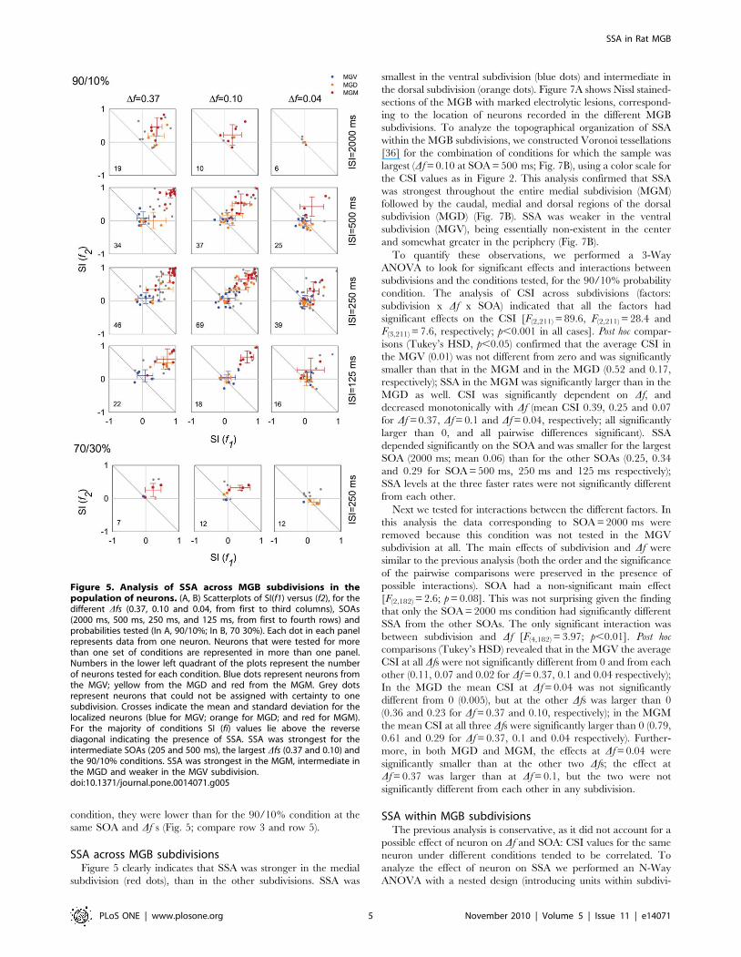
SSA across MGB subdivisionsFigure 5 clearly indicates that SSA was stronger in the medial
subdivision (red dots), than in the other subdivisions. SSA was
smallest in the ventral subdivision (blue dots) and intermediate in
the dorsal subdivision (orange dots). Figure 7A shows Nissl stained-
sections of the MGB with marked electrolytic lesions, correspond-
ing to the location of neurons recorded in the different MGB
subdivisions. To analyze the topographical organization of SSA
within the MGB subdivisions, we constructed Voronoi tessellations
[36] for the combination of conditions for which the sample was
largest (Df = 0.10 at SOA = 500 ms; Fig. 7B), using a color scale for
the CSI values as in Figure 2. This analysis confirmed that SSA
was strongest throughout the entire medial subdivision (MGM)
followed by the caudal, medial and dorsal regions of the dorsal
subdivision (MGD) (Fig. 7B). SSA was weaker in the ventral
subdivision (MGV), being essentially non-existent in the center
and somewhat greater in the periphery (Fig. 7B).
To quantify these observations, we performed a 3-Way
ANOVA to look for significant effects and interactions between
subdivisions and the conditions tested, for the 90/10% probability
condition. The analysis of CSI across subdivisions (factors:
subdivision x Df x SOA) indicated that all the factors had
significant effects on the CSI [F(2,211) = 89.6, F(2,211) = 28.4 and
F(3,211) = 7.6, respectively; p,0.001 in all cases]. Post hoc compar-
isons (Tukey’s HSD, p,0.05) confirmed that the average CSI in
the MGV (0.01) was not different from zero and was significantly
smaller than that in the MGM and in the MGD (0.52 and 0.17,
respectively); SSA in the MGM was significantly larger than in the
MGD as well. CSI was significantly dependent on Df, and
decreased monotonically with Df (mean CSI 0.39, 0.25 and 0.07
for Df = 0.37, Df = 0.1 and Df = 0.04, respectively; all significantly
larger than 0, and all pairwise differences significant). SSA
depended significantly on the SOA and was smaller for the largest
SOA (2000 ms; mean 0.06) than for the other SOAs (0.25, 0.34
and 0.29 for SOA = 500 ms, 250 ms and 125 ms respectively);
SSA levels at the three faster rates were not significantly different
from each other.
Next we tested for interactions between the different factors. In
this analysis the data corresponding to SOA = 2000 ms were
removed because this condition was not tested in the MGV
subdivision at all. The main effects of subdivision and Df were
similar to the previous analysis (both the order and the significance
of the pairwise comparisons were preserved in the presence of
possible interactions). SOA had a non-significant main effect
[F(2,182) = 2.6; p = 0.08]. This was not surprising given the finding
that only the SOA = 2000 ms condition had significantly different
SSA from the other SOAs. The only significant interaction was
between subdivision and Df [F(4,182) = 3.97; p,0.01]. Post hoc
comparisons (Tukey’s HSD) revealed that in the MGV the average
CSI at all Dfs were not significantly different from 0 and from each
other (0.11, 0.07 and 0.02 for Df = 0.37, 0.1 and 0.04 respectively);
In the MGD the mean CSI at Df = 0.04 was not significantly
different from 0 (0.005), but at the other Dfs was larger than 0
(0.36 and 0.23 for Df = 0.37 and 0.10, respectively); in the MGM
the mean CSI at all three Dfs were significantly larger than 0 (0.79,
0.61 and 0.29 for Df = 0.37, 0.1 and 0.04 respectively). Further-
more, in both MGD and MGM, the effects at Df = 0.04 were
significantly smaller than at the other two Dfs; the effect at
Df = 0.37 was larger than at Df = 0.1, but the two were not
significantly different from each other in any subdivision.
SSA within MGB subdivisionsThe previous analysis is conservative, as it did not account for a
possible effect of neuron on Df and SOA: CSI values for the same
neuron under different conditions tended to be correlated. To
analyze the effect of neuron on SSA we performed an N-Way
ANOVA with a nested design (introducing units within subdivi-
Figure 5. Analysis of SSA across MGB subdivisions in thepopulation of neurons. (A, B) Scatterplots of SI(f1) versus (f2), for thedifferent Dfs (0.37, 0.10 and 0.04, from first to third columns), SOAs(2000 ms, 500 ms, 250 ms, and 125 ms, from first to fourth rows) andprobabilities tested (In A, 90/10%; In B, 70 30%). Each dot in each panelrepresents data from one neuron. Neurons that were tested for morethan one set of conditions are represented in more than one panel.Numbers in the lower left quadrant of the plots represent the numberof neurons tested for each condition. Blue dots represent neurons fromthe MGV; yellow from the MGD and red from the MGM. Grey dotsrepresent neurons that could not be assigned with certainty to onesubdivision. Crosses indicate the mean and standard deviation for thelocalized neurons (blue for MGV; orange for MGD; and red for MGM).For the majority of conditions SI (fi) values lie above the reversediagonal indicating the presence of SSA. SSA was strongest for theintermediate SOAs (205 and 500 ms), the largest Dfs (0.37 and 0.10) andthe 90/10% conditions. SSA was strongest in the MGM, intermediate inthe MGD and weaker in the MGV subdivision.doi:10.1371/journal.pone.0014071.g005
SSA in Rat MGB
PLoS ONE | www.plosone.org 5 November 2010 | Volume 5 | Issue 11 | e14071
sions). This analysis demonstrated a strong effect of neuron on the
variation of SSA (F(73,138) = 5.26; p,0.0001).
To look at the effects of neuron, Df, and SOA on SSA within
subdivisions, we performed 3-Way ANOVAs for each subdivision
separately, with the neurons as a random factor. This analysis
demonstrated a significant effect of neurons in each subdivision
separately [F(21,39) = 2.75; p,0.01; F(28,34) = 14.92; p,0.001; and
F(24,56) = 3.10; p,0.001, for the MGV, MGD and MGM
respectively]. Within subdivisions, after controlling for neuron,
the effect of Df was not significant in the ventral and dorsal
subdivisions [F(2,21) = 2.06; p = 0.1 and F(2,34) = 1.69; p = 0.2,
respectively], but was significant in the medial subdivision
[F(2,56) = 5.06; p,0.01]. These results are consistent with the
analysis of the interactions between Df and subdivision presented
above, which showed that the effect of Df was more pronounced in
the MGM, weaker in the MGD and absent in the MGV. Most
importantly, the analysis within subdivisions reveals a strong effect
of SOA. CSI had a monotonically-inverse relationship with SOA
in all three subdivions [F(2,39) = 5.49; p,0.01; F(3,34) = 21.78;
p,0.001; and F(3,56) = 10.47; p,0.001, for the MGV, MGD and
MGM respectively].
Post hoc comparisons showed that in the MGV, SSA at the
shortest SOA (125 ms) was significantly larger than at
SOA = 250 ms; the other comparisons were not significant.
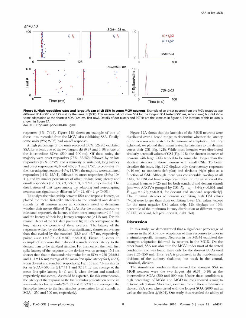
Figure 8 shows an example of a neuron, localized to the MGV,
that exhibited SSA at SOA = 125 (CSI = 0.34; first row) but not at
SOA = 250 ms (CSI = 0.03; not shown) or SOA = 500 ms
(CSI = 0.03; second row).
In the MGD, as in the MGV, SSA at SOA of 125 ms was
significantly larger than at 250 ms. In the MGM, on the other
hand, there was no significant difference between SOAs of 125,
250 and 500 ms. Figure 4 shows an example of a neuron, localized
to the MGM, that exhibited the same degree of adaptation for all
of these different SOAs (first, second and third rows; 125, 250 and
500 ms, respectively).
In the MGD and the MGM, SSA at the longest SOA (2000 ms)
was significantly reduced with respect to the other SOAs. Figure 9
shows an example of a neuron, localized to the MGM, that
showed reduced CSI at the longest SOA (second row in A and B)
compared to shorter SOAs (first row in A and B), for two different
Dfs (0.37 and 0.10).
Time course of SSAIn order to study the dynamics of SSA in the population of
MGB neurons, we calculated the average population firing rate
versus trial number, for the two SOA conditions that showed the
highest levels of adaptation (SOA = 250 and 500 ms), and for
which we collected the most data (Figure 10). We analyzed
separately the non-adapting neurons (CSI#0.18) and the adapting
neurons (CSI.0.18) (Fig. 10 A and B; left and right columns,
respectively). In the initial trials, the average responses to the
standard and deviant stimuli were similar (Fig. 10). The adapting
neurons maintained or only slightly reduced their response to the
deviant stimulus through the trials, while the response to the
standard declined more strongly after the first few trials (Figs. 10;
right column). The responses of non-adapting neurons to the
standard also showed some decrement after the first trials,
especially for the Df = 0.37 conditions (Fig. 10; left column), but
this decrement was much smaller than that of the adapting
neurons. As a consequence, non-adapting neurons maintained a
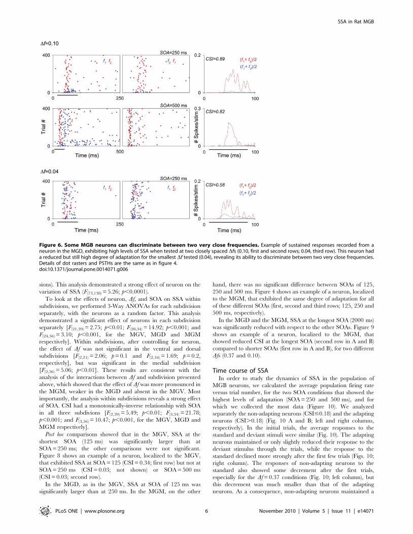
Figure 6. Some MGB neurons can discriminate between two very close frequencies. Example of sustained responses recorded from aneuron in the MGD, exhibiting high levels of SSA when tested at two closely spaced Dfs (0.10, first and second rows; 0.04, third row). This neuron hada reduced but still high degree of adaptation for the smallest Df tested (0.04), revealing its ability to discriminate between two very close frequencies.Details of dot rasters and PSTHs are the same as in figure 4.doi:10.1371/journal.pone.0014071.g006
SSA in Rat MGB
PLoS ONE | www.plosone.org 6 November 2010 | Volume 5 | Issue 11 | e14071

higher firing rate to the standard than the adapting neurons across
the trials, for all conditions (Fig. 10). We then fitted the responses to
the standard with an exponential decay regression model [f = a*exp(-
b*x)] and a polynomial inverse first order regression model
[f = y0+(a/x)]. The polynomial inverse first order model was the
one that provided the best fit to the responses to the standard across
trials, for all conditions. A high proportion of the adaptation to the
standard by the adapting neurons was explained by this model, for
the majority of conditions (SOA = 250 ms: r2 = 0.68 and 0.64, at
Df = 0.37 and 0.10, respectively; SOA = 500 ms: r2 = 0.47 at both
Dfs; p,0.001 for all conditions; Fig. 10A and B, respectively; right
column, first and second rows). For the smallest Df (0.04) the
variance explained by the model was reduced (r2 = 0.24, 0.20 at
SOA = 250 and 500 ms, respectively; p,0.001 for both conditions;
Fig. 10, right column, third row). For the non-adapting neurons, the
variance explained by the model was very low for all conditions
(SOA = 250 ms: r2 = 0.04, 0.12 and 0.1, for Df = 0.37, 0.1 and 0.04,
respectively; SOA = 500 ms: r2 = 0.14, 0.05 and 0.12, for Df = 0.37,
0.1 and 0.04, respectively; p,0.001 for all conditions; Fig. 10, left
column). The smaller amount of variance explained by the
regression model in these conditions presumably reflects the minor
amount of adaptation of the non-adapting neurons.
SSA in relation to discharge patterns and latenciesOver half of the neurons that we recorded from the MGB had
onset responses to auditory stimuli (53%; 49/93, e.g., Figs. 4, 8 and
9) while 24% had sustained responses (22/93, e.g., Fig. 6; defined
as neurons that responded for 50 ms or more [23,25], in response
to a 75 ms stimulus). In addition, some units (10%; 9/93) had two
different response components: a brief onset burst at a relatively
short latency (10–30 ms) followed by a long-duration burst at a
much longer latency (.115 ms). Both response components were
tuned to the same frequency range, but were clearly segregated in
time. We refer to these units as on-late units. Fig. 11A shows an
example of one of these units, recorded from the MGD and
exhibiting SSA. A small percentage of neurons had offset
Figure 7. Location of recorded neurons and topographical organization of SSA across the MGB. (A) Nissl stained sections showing theMGB in the transverse plane. On the left (caudal), arrows indicate the electrolytic lesion in the MGM marking the recording site of the neuron shownin figure 9. Asterisk indicates another lesion for reference. On the right (rostral), arrows indicate an electrolytic lesion in the MGD and another one inthe MGV, marking the recording site of the neuron shown in figure 8. Asterisk shows the recording track. D, dorsal; L, lateral; Calibration bar =500 mm. (B) Topographical organization of SSA within the MGB subdivisions, for the Df = 0.10 at SOA = 500 ms condition. The center of tessellatedpolygons in the maps represents the sites at which the neurons were recorded. Each polygon was colored according to the CSI value of the neuronrecorded at that site. The bar on the right represents the color scale used for the CSI range. Both the transverse projection (on left) and the horizontalprojections through the MGV/MGM (section 1) and MGD (section 2) show that SSA was strongest throughout the entire MGM followed by the caudal,medial and dorsal regions of the MGD. SSA was very weak in the center of the MGV, but somewhat greater in its periphery.doi:10.1371/journal.pone.0014071.g007
SSA in Rat MGB
PLoS ONE | www.plosone.org 7 November 2010 | Volume 5 | Issue 11 | e14071
responses (8%; 7/93). Figure 11B shows an example of one of
these units, recorded from the MGV, also exhibiting SSA. Finally,
some units (2%; 2/93) had on-off responses.
A high percentage of the units recorded (56%; 52/93) exhibited
SSA for at least one of the two largest Dfs (0.37 and 0.10) at one of
the intermediate SOAs (250 and 500 ms). Of these units, the
majority were onset responders (73%; 38/52), followed by on-late
responders (12%; 6/52), and a minority of sustained, long latency
and offset responders (6, 6 and 4%; 3, 3 and 2/52, respectively). Of
the non-adapting neurons (44%; 41/93), the majority were sustained
responders (44%; 18/41), followed by onset responders (24%; 10/
41), and by smaller percentages of offset, on-late, long latency and
on-off responders (12, 7.3, 7.3, 5%; 5, 3, 3, 2/41, respectively). The
distributions of unit types among the adapting and non-adapting
neurons was significantly different (x2 = 22, df = 2, p,0.001).
To analyze the relationship between SSA and response latency, we
plotted the mean first-spike latencies to the standard and deviant
stimuli for all neurons under all conditions tested to determine
whether their means differed (Fig. 12A). For the on-late neurons, we
calculated separately the latency of their onset component (,115 ms)
and the latency of their long latency component (.115 ms). For this
reason, 16 out of the 388 data points in figure 12A correspond to the
long latency components of these neurons. The latency of the
responses evoked by the deviant was significantly shorter on average
than that evoked by the standard (42.9 and 45.7 ms, respectively;
paired t-test: t = 5.79, d.f. = 387, p,0.001). Figure 13 shows an
example of a neuron that exhibited a much shorter latency to the
deviant than to the standard stimulus. For this neuron, the mean first
spike latency of the response to the deviant was on average 15.1 ms
shorter than that to the standard stimulus for an SOA = 250 (2660.4
and 41.161.6 ms; average of the mean first-spike latency for f1 and f2when deviant and standard, respectively; Fig. 13); and 7.6 ms shorter
for an SOA = 500 ms (24.761.1 and 32.361.2 ms; average of the
mean first-spike latency for f1 and f2 when deviant and standard,
respectively; not shown). As would be expected, for this same neuron,
the latency of the response to the first stimulus presentation of the set
was similar for both stimuli (2460.7 and 23.560.3 ms, average of the
first-spike latency to the first stimulus presentation for all stimuli, at
SOA = 250 and 500 ms, respectively).
Figure 12A shows that the latencies of the MGB neurons were
distributed over a broad range; to determine whether the latency
of the neurons was related to the amount of adaptation that they
exhibited, we plotted their mean first-spike latencies to the deviant
versus their CSI (Fig. 12B). While most latencies were distributed
similarly across all values of CSI (Fig. 12B), the shortest latencies of
neurons with large CSIs tended to be somewhat longer than the
shortest latencies of those neurons with small CSIs. To better
visualize this issue, Fig. 12C displays only short-latency responses
(,40 ms) to standards (left plot) and deviants (right plot) as a
function of CSI. Although there was considerable overlap at all
CSIs, the CSI did have a significant effect on the variation of the
minimal latencies (,25 ms) for both standard and deviant stimuli
[one-way ANOVA grouped by CSI: F(11,171) = 3.64; p,0.001; and
F(11,203) = 4.72; p,0.001, for deviant and standard respectively].
The minimal latencies of neurons exhibiting high CSI values
(.0.5) were longer than those exhibiting lower CSI values, except
for the most negative CSI values (Fig. 12E displays the 10%
percentile of the minimum latency distribution at different ranges
of CSI; standard, left plot; deviant, right plot).
Discussion
In this study, we demonstrated that a significant percentage of
neurons in the MGB show adaptation of their responses to tones in
a stimulus-specific manner. Neurons in the MGM exhibited the
strongest adaptation followed by neurons in the MGD. On the
other hand, SSA was absent in the MGV under most of the tested
conditions, and was found there only for the shortest SOAs used
here (125–250 ms). Thus, SSA is prominent in the non-lemniscal
divisions of the auditory thalamus, but weak in the ventral,
lemniscal, division.
The stimulation conditions that evoked the strongest SSA in
MGB neurons were the two largest Dfs (0.37, 0.10) at the
intermediate SOAs (250 and 500 ms). Under these conditions a
high percentage of MGM and MGD neurons showed strong to
extreme adaptation. Moreover, some neurons in these subdivisions
showed SSA even when tested with the longest SOA (2000 ms) as
well as the smallest Df (0.04). Our study thus revealed the ability of
Figure 8. High repetition rates and large Dfs can elicit SSA in some MGV neurons. Example of an onset neuron from the MGV tested at twodifferent SOAs (500 and 125 ms) for the same Df (0.37). This neuron did not show SSA for the longest SOA tested (500 ms, second row) but did showsome adaptation at the shortest SOA (125 ms, first row). Details of dot rasters and PSTHs are the same as in figure 4. The location of this neuron isshown in figure 7A.doi:10.1371/journal.pone.0014071.g008
SSA in Rat MGB
PLoS ONE | www.plosone.org 8 November 2010 | Volume 5 | Issue 11 | e14071

these neurons to discriminate between two very close frequencies,
both of which are well within their frequency response area. Such
hyperacuity was demonstrated before in cat AC [10] and rat IC
[4]. Our results together with those of others [1,4,10,12,13]
demonstrate the ubiquity of SSA in neurons throughout the
auditory system, from the midbrain up to the auditory cortex.
Comparison with previous studiesTwo recent studies tested SSA in MGB. Yu and colleagues [13]
studied SSA in the rat MGB and thalamic reticular nucleus, a
subdivision of the thalamus that lies outside the MGB. They
demonstrated strong SSA in the thalamic reticular nucleus and
weaker SSA in MGB. Anderson and colleagues [1] reported SSA in
mouse MGB, but tested fewer conditions and showed weaker SSA
than reported in the current study. We demonstrated that some
neurons in the rat MGB exhibit very strong SSA even under the
most extreme conditions tested (SOAs = 2000 ms or Df = 0.04). In
fact, we found a few neurons in MGB with CSI values as high as
those reported by Yu et al. [13] in the thalamic reticular nucleus,
even when using SOAs twice as long.
Figure 9. Low repetition rates elicit high SSA in some MGM neurons. Example of an onset neuron with spontaneous activity recorded in the MGM,showing strong adaptation under all of the conditions tested. (A) the neuron exhibited extreme adaptation when tested at the same SOA (500 ms) for two different Dfs(0.37 and 0.10; first and second rows, respectively). (B) the neuron showed somewhat lower adaptation when tested at the longest SOA (2000 ms; same Dfs as in A). In bothA and B, the adaptation was similar for both Df conditions. Details of dot rasters and PSTHs are the same as in figure 4. The location of this neuron is shown in figure 7A.doi:10.1371/journal.pone.0014071.g009
SSA in Rat MGB
PLoS ONE | www.plosone.org 9 November 2010 | Volume 5 | Issue 11 | e14071

The parameter ranges over which SSA occurs in the rat MGB are
similar to those in cat AC [10] and rat IC [4]. SSA in the rat IC was
tested only for relatively short SOAs (up to 500 ms), so we cannot
compare the IC with the MGB for the largest SOA. However, our
MGB results (SOA = 2000 ms, inter-tone duration.1900 ms) can
be compared with those from the cat AC study (SOA = 2000 ms,
inter-tone duration.1700 ms). A SOA of 2000 ms corresponds to
the most extreme condition for which Ulanovsky and colleagues
[10] showed single units exhibiting SSA in A1 (CSI<0.3). We found
higher values of SSA for this condition in the MGB (up to CSI = 0.7)
than the previous study in the AC, but only outside the MGV. The
MGV receives input from the central nucleus of the IC and is the
main source of ascending input to A1 [28–31]. In this context, it is
worth mentioning that SSA found in the central nucleus of the IC
[4] is only relatively large for the shortest SOA tested (125 ms).
Thus, the MGB and IC data tightly links SSA in subcortical regions
to the non-lemniscal pathway [4,6].
CSI values reported in A1 of the cat are far in excess of the
values measured in cat MGB, presumably in the ventral division
[10], or in rat MGV. Thus, our results suggest that A1 is the first
lemniscal station in which SSA is widespread and strong. SSA in
A1 may therefore express the combined result of the rather weak
SSA found in MGV augmented by intracortical mechanisms [37]
and possibly by the weaker (but still present) non-lemniscal input
to A1, either directly from the MGM [38] or indirectly through
feedback connections from higher auditory areas. For example, a
recent study [39] has demonstrated that reversible thermal
deactivation of AAF alters A1 responses but AAF responses are
not altered by A1 deactivation. These authors suggest a
unidirectional flow of information from the non-lemniscal to the
lemniscal pathway. If so, the SSA observed in A1 may be
modulated by the influence of AAF [10].
Strongly adapting neurons in both the MGB and the IC [4,6] were
mainly onset responders, with relatively short latencies (,40 ms) for
both the standard and the deviant stimuli. Nevertheless, the shortest
latencies of the neurons that showed strong adaptation for a certain
condition in the MGB were significantly longer than those of weakly
adapting neurons for a certain condition, to both the deviant and
standard stimuli. These slightly longer latencies could simply reflect
lower firing rates of the neurons showing strong adaptation for a given
condition, as the mean first-spike latency can be affected by the
response strength, or it could be due to additional neuronal
processing, for example cortical modulation of these neurons [10].
This hypothesis needs to be addressed in future experiments, e.g., by
reversibly inactivating the AC [40,41].
SSA and sensory memoryA neuron exhibiting SSA integrates information about recent
stimulus history in order to respond more strongly to a rare
stimulus. SSA therefore embodies a short-term memory trace that
determines the response of the neuron to subsequent stimulation
[7,42,43]. We demonstrated that a polynomial scale-invariant
model explained a high proportion of MGB neurons’ adaptation
to the standard stimulus. Such a power law model may indicate
that adaptation occurs over a range of time-scales [44,45], so that
in contrast to exponential adaptation, activity more than a few
time constants back, although deemphasized, is not discarded.
Indeed, SSA in A1 neurons appears to occur on several time scales
concurrently, spanning many orders of magnitude, from hundreds
of milliseconds to tens of seconds [11], paralleling the behaviour of
large neuronal populations as recorded in human event-related
potentials [46]. SSA was therefore proposed as a candidate
neuronal mechanism for auditory sensory memory and deviance
detection as reported in human MMN studies [5,47,48]. However,
Figure 10. Time course of adaptation in the population of MGBneurons. Average population firing rate (spikes/stimulus) versus trialnumber for SOA = 250 ms (A) and SOA = 500 ms (B) and the differentDfs tested, indicated to the right of each row. In both A and B, the leftcolumns correspond to non-adapting neurons (CSI#0.18) and rightcolumns to adapting neurons (CSI.0.18). The response of the adaptingneurons to the standard stimulus strongly declined after the first trials.A high proportion of their adaptation to the stimulus was explained bya polynomial inverse regression model [f = y0+(a/x)], for the majority ofconditions; the amount of variance explained was reduced for thesmallest Df (0.04) (r2 = 0.24, 0.20 in A and B, respectively; p ,0.001 forboth conditions) and was very low for the non-adapting neurons, underall conditions.doi:10.1371/journal.pone.0014071.g010
SSA in Rat MGB
PLoS ONE | www.plosone.org 10 November 2010 | Volume 5 | Issue 11 | e14071

the MMN component occurs at 100–250 ms after the onset of an
acoustic change, while SSA occurs at much shorter latencies
[4,11]. Indeed, a recent study based on neuronal recordings and
evoked local field potentials (eLFP) in the awake rat found
enhanced responses to deviants in eLFP but did not find the late
deviant response component that would have been the equivalent
to the human MMN [12]. Thus, SSA has been suggested to lie
upstream of MMN generation. Recent studies in humans
demonstrated that deviance detection can take place as early as
30 ms after stimulus onset, suggesting that early change detection
processes occur upstream of MMN generation [49,50]. As in the
animal models that have been studied, deviance detection in
humans occurs at multiple levels in the auditory pathway, from the
brainstem up to higher-order cortical areas [49,50].
Here, we demonstrate that the latencies of strongly adapting
neurons in the MGB span a range between approximately 10 ms to
250 ms [51], covering the range of the different components of the
MMN in humans [47,49,50] and rats [52,53]. The majority of the
strongly adapting neurons in the MGM subdivision had onset
responses with short latencies. These neurons could be participants
in a bottom-up stream of SSA [51]. However, some strongly adapting
neurons in the MGB had very long onset latencies (.150 ms) and
some neurons had two different components in their response, i.e., a
short latency component (,40 ms) together with a long latency one
(.150 ms). The timing of the long latency components of these
neurons is similar to the range of the latencies of the MMN component
of human ERPs (<200 ms; [14,47,54]). This suggests that there might
be some relationship between the SSA exhibited by this population of
neurons and the MMN component. Our data and those of others who
found evidence of MMN subcortically (reviewed in [19]) indicate that
MMN may be generated by processes that include both bottom-up
processing and corticothalamic feedback loops.
The presence of strong SSA in the auditory thalamus suggests
that SSA is important for the type of processing performed there.
For example, the very strong SSA found in the MGM is consistent
with its role as a major auditory input to the fear circuit in the
amygdala [24,55]. The role of SSA expressed in IC and MGB in
shaping SSA in A1 is less clear, and it may well be that SSA in A1 is
generated at least in part de-novo. Nevertheless, the presence of
strongly-adapting neurons in non-lemniscal divisions of the MGB
may indicate the active role of these neurons in the generation,
transformation or modulation of SSA expressed in other parts of the
auditory system. Testing such a role would require future work.
Materials and Methods
Surgical proceduresExperiments were performed on 21 adult rats with body weights
between 150–250 g. All experiments were carried out at the
University of Salamanca with the approval of, and using methods
conforming to the standards of, the University of Salamanca
Animal Care Committee.
Surgical anaesthesia was induced and maintained with urethane
(1.5 g/kg, i.p.), with supplementary doses (0.5 g/kg, i.p.) given as
needed. Urethane was selected as an anaesthetic because its effects
on multiple aspects of neural activity, including inhibition and
spontaneous firing, are known to be less than those of barbiturates
and other anaesthetic drugs (e.g. [56]). The trachea was
cannulated, and atropine sulphate (0.05 mg/kg, s.c.) was admin-
istered to reduce bronchial secretions. Body temperature was
maintained at 38uC61uC. Details of surgical preparation were as
described elsewhere [57,58]. The animal was placed in a
stereotaxic frame in which the ear bars were replaced by hollow
specula that accommodated a sound delivery system.
Acoustic stimuli and electrophysiological recordingA craniotomy was performed to expose the cerebral cortex
overlying the MGB. A tungsten electrode (1–2 MV; [59]) was
Figure 11. Some MGB neurons with on-late and off response types show adaptation. (A) Example of an on-late neuron in the MGD. Thisneuron responded with a brief onset burst at a relatively short latency (14.860.4 and 1660.5 ms; average of the mean first-spike latency for f1and f2 when deviant and standard, respectively) followed by a long-duration burst at a much longer latency (245.867 ms; average of the mean first-spike latency for f1 and f2 when deviant). The neuron showed some adaptation in the onset burst but much stronger adaptation in the late burst(CSI = 0.31 and 0.98, respectively; CSI = 0.57 for the entire response time window). Details of dot rasters and PSTHs are the same as in figure 4.(B) Example of an offset neuron from the MGV that exhibited some adaptation (CSI = 0.26). Details of dot rasters and PSTHs are the same as in figure 4.doi:10.1371/journal.pone.0014071.g011
SSA in Rat MGB
PLoS ONE | www.plosone.org 11 November 2010 | Volume 5 | Issue 11 | e14071

lowered through the cortex and used to record extracellular single
unit responses. Neuron localization in the MGB was based on
stereotaxic coordinates, physiological criteria of tonotopicity and
response properties [23–25]. Subsequent histological verification
was performed using electrolytic lesions (5–10 mA for 5–10 s) to
mark recording sites [60].
Stimuli were delivered through a sealed acoustic system [61,62]
using two electrostatic loudspeakers (TDT- EC1) driven by two
TDT-ED1 modules. Pure tone bursts were delivered to the
contralateral ear under computer control using TDT System 2
(Tucker-Davis Technologies) hardware and custom software
[4,63,64]. The output of the system at each ear was calibrated
in situ using a J’’ condenser microphone (Bruel and Kjær 4136,
Nærum, Denmark) and a DI-2200 spectrum analyser (Diagnostic
Instruments Ltd., Livingston, Scotland, UK). The maximum
output of the TDT system was flat from 0.3–5 kHz (,10067 dB
Figure 12. Response latencies in the MGB population of neurons. (A) Mean first-spike latencies to the deviant versus standard stimulus for theMGB population. Latencies to the deviant were on average significantly shorter than those to the standard stimulus (Mean = 42.9 and 45.7 ms,respectively; paired t-test: t = 5.79, n = 388, d.f = 387, p,0.001). (B) Mean first-spike latencies to the deviant versus CSI. The shortest latencies o f highlyadapting neurons were longer than those of non-adapting neurons. (C) Short-latency responses (,40 ms) to standard (left plot) and deviant (right plot)versus CSI. (D) The 10th percentile of the minimum latency distribution for the standard (left plot) and deviant (right plot) at different ranges of CSI. Theminimal latencies of neurons with high CSI values (.0.5) were longer than those with lower CSI values, except for the most negative CSI values.doi:10.1371/journal.pone.0014071.g012
SSA in Rat MGB
PLoS ONE | www.plosone.org 12 November 2010 | Volume 5 | Issue 11 | e14071

SPL) and from 5–40 kHz (9065 dB SPL). The highest frequency
produced by this system was limited to 40 kHz. The second and
third harmonic components in the signal were 40 dB or more
below the level of the fundamental at the highest output level
[60,65].
Tones were 75 ms duration with a 5 ms rise/fall time. The
electrode was advanced using a Burleigh microdrive. Action
potentials were recorded with a BIOAMP amplifier (TDT), the
10X output of which was further amplified and bandpass-filtered
(TDT PC1; fc, 500 Hz and 3 kHz) before passing through a spike
discriminator (TDT SD1). Spike times were logged on a computer
by feeding the output of the spike discriminator into an event timer
(TDT ET1) synchronized to a timing generator (TDT TG6).
Stimulus generation and on-line data visualization were controlled
with custom software. Spike times were displayed as dot rasters
ordered by the acoustic parameter varied during testing. Search
stimuli were pure tones or noise bursts.
To the extent possible, the approximate frequency tuning of the
cell was audiovisually determined. The minimum threshold and
best frequency (BF) of the cell were obtained by an automated
procedure with 2–5 stimulus repetitions at each frequency and
intensity step. The monaural frequency response area (FRA, e.g.,
Fig. 1), i.e., the combination of frequencies and intensities capable
of evoking a response, was then obtained automatically using a
randomized stimulus presentation paradigm and plotted using
EXCEL, SIGMAPLOT and MATLAB software. The stimuli used
to generate FRAs in single units were pure tones with a duration of
75 ms. Frequency and intensity of the stimulus were varied
randomly (0–100 dB attenuation in 5 or 10 dB steps and in 25
frequency steps from 0.1–40 to cover approximately 2–3 octaves
above and below the BF; [60,65]).
Stimulus presentation paradigmsFor all neurons, stimuli were presented in an oddball paradigm
similar to that used to record mismatch negativity responses in
human studies [54] and more recently in the cat auditory cortex
[10,11] and rat inferior colliculus [4]. Briefly, we presented trains
of two different pure tone stimuli (f1 and f2), at a level of 10–40 dB
above threshold. Both frequencies were within the excitatory
frequency response area previously determined for the neuron
(Fig. 1). We presented a train of 400 stimuli containing both
frequencies in a pseudo-random order at a specific repetition rate.
One frequency (f1) was presented as the standard (i.e., high
probability within the sequence); interspersed randomly with the
second frequency (f2) presented as the deviant (i.e., low probability
within the sequence). Special care was taken to choose a frequency
pair that elicited similar spike counts when presented individually,
to ensure that all differences in response were solely due to the
statistics of the stimulus ensemble (Fig. 1). The custom software
allowed us to independently vary the probability of the deviant
stimulus and the amount by which its frequency varied from that
of the standard. After obtaining one data set, the relative
probabilities of the two stimuli were reversed, with f2 as the
standard and f1 as the deviant (total number of stimuli for the
frequency pair, 800).
The same paradigm was repeated varying the probability of the
standard/deviant stimuli (90/10% and 70/30%), the stimulus
onset asynchrony (SOA = 2000 ms, 500 ms, 250 ms, and 125 ms),
and the frequency contrast between the standard and deviant. The
frequency contrasts were chosen to be as close as possible to values
that have been used in other studies to allow direct comparisons
of the data [4,10,11], i.e., Df = 0.37, 0.10 and 0.04; where
Df = (f22f1)/(f2*f1)1/2 is the normalized frequency difference
(Malmierca et al., 2009;Ulanovsky et al., 2003). These values
correspond to frequency ratios of 0.526, 0.141 and 0.057 octaves,
respectively. We quantified SSA as described previously [4,10,11].
The frequency-specific SSA index, SI(fi) (i = 1 or 2), was calculated
as SI(fi) = [d(fi)2s(fi)]/[d(fi)+s(fi)] where d(fi) and s(fi) were responses
(in spike counts/stimulus) to frequency fi when it was deviant or
standard, respectively. The amount of SSA for both frequencies at
each condition (Common SSA index, CSI) was calculated as
CSI = [d(f1)+d(f2)2s(f1)2s(f2)]/[d(f1)+d(f2)+s(f1)+s(f2)].
These indices reflect the extent to which the response to a tone,
when standard, was smaller than the response to the same tone,
when deviant. The indices range between 21 to +1, being positive
if the response to a tone, when deviant, was greater than the
response to the same tone, when standard. To thoroughly quantify
the conditions that elicited SSA in a given neuron, the indices were
calculated for the different combination of conditions tested
(probability ratios, frequency contrasts, and repetition rates). For
each neuron, this resulted in a set of SI(fi) and CSI values for all of
the conditions that were tested.
To analyse SSA across MGB subdivisions, a fixed-effect 3-way
ANOVA was performed (factors: subdivisions x Df x SOA),
followed by Post hoc comparisons (Tukey’s HSD, p,0.05). To
analyse the effect of neuron on SSA the 3-way ANOVA was
augmented into a nested design (neurons within subdivisions). To
analyse the effects of neuron, Df and SOA on SSA within
subdivisions, 3-Way ANOVAs were performed for each subdivi-
sion separately, with neurons considered as a random factor. All
Figure 13. MGB neurons show shorter latencies to the deviant than to the standard stimulus. Example of an adapting neuron thatresponded with a much shorter latency to the deviant than to the standard stimulus (2660.4 and 41.161.6 ms; average of the mean first-spikelatency between f1 and f2 when deviant and standard, respectively), for a Df = 0.10 at SOA = 250 ms condition. The latency of the response to thefirst stimulus presentation of the set was similar for both stimuli, it was even slightly shorter to the standard (24.560.7 and 23.560.2 ms, average ofthe first-spike latency to the first stimulus presentation between f1 and f2, when deviant and standard, respectively). Details of dot rasters and PSTHsare the same as in figure 4.doi:10.1371/journal.pone.0014071.g013
SSA in Rat MGB
PLoS ONE | www.plosone.org 13 November 2010 | Volume 5 | Issue 11 | e14071
analyses were done using the statistical toolbox of Matlab
(MathWorks).
Histological verification of recording sitesEach track was marked with electrolytic lesions for subsequent
histological localization of the neurons recorded. At the end of
most experiments (26 out of 34) the animal was given a lethal dose
of sodium pentobarbital and perfused transcardially with phos-
phate buffered saline (0.5% NaNO3 in PBS) followed by fixative
(a mixture of 1% paraformaldehyde and 1% glutaraldehyde in rat
Ringer’s solution). After fixation and dissection, the brain tissue
was cryoprotected in 30% sucrose and sectioned on a freezing
microtome in the transverse or sagittal planes into 40 mm-thick
sections. Sections were Nissl stained with 0.1% cresyl violet to
facilitate identification of cytoarchitectural boundaries [22].
Recording sites were marked on standard sections from a rat
brain atlas [65] and units were assigned to one of the three main
divisions (ventral, dorsal and medial) of the MGB [22]. The
stained sections with the lesions were used to localize each track
mediolaterally, dorsoventrally and rostrocaudally in the Paxinos
atlas [66]. To determine the three main MGB subdivisions [20,22]
cytoarchitectonic criteria, i.e., cell shape and size, Nissl staining
patterns and cell packing density, were used. This information was
complemented and confirmed by the stereotaxic coordinates used
during the experiment to localize the MGB. After assigning a
section to each track/lesion, the electrophysiological coordinates
from each experiment and recording unit, i.e., beginning and end
of the MGB, as well as the depth of the neuron, were used as
complementary references to localize each neuron within a track.
Neurons localized at the border between subdivisions and those
recorded in the animals that were not perfused were excluded
from this analysis. Based on selected conditions for which a large
number of tested neurons were localized, topographic maps of
SSA were constructed using Voronoi Tessellations of the recording
sites (e.g. [36]). Each polygon was coloured according to the CSI
of the unit recorded at that site. The sections shown in figure 7A
were photographed at high resolution with a Zeiss Axioskop 40
microscope using a Zeiss AxioCam MRc 5 digital camera (Carl
Zeiss, Oberkochen, Germany) and plan semi-apochromatic
objective lenses 56 (NA 0.15). The brightness and contrast of
images were adjusted with Adobe Photoshop software (Adobe, San
Jose, CA, USA).
Acknowledgments
We thank David Perez-Gonzalez and Jorge Martin for their assistance on
figure 2 and 7B, Enrique Saldana for his help in taking the
photomicrographs on Fig. 7A and Ignacio Plaza for his help with
histological processing. We also thank 3 anonymous reviewers for their
critical and constructive criticisms.
Author Contributions
Conceived and designed the experiments: EC MSM. Performed the
experiments: FMA. Analyzed the data: FMA IN. Contributed reagents/
materials/analysis tools: FMA IN EC. Wrote the paper: FMA MSM.
Supervised the project: MSM. Gave conceptual advice: IN EC.
References
1. Anderson LA, Christianson GB, Linden JF (2009) Stimulus-specific adaptation
occurs in the auditory thalamus. J Neurosci 29: 7359–7363.
2. Baeuerle P, Von Der Behrens W, Gaese B, Kossl M (2009) Stimulus-Specific
Adaptation in the Auditory Thalamus of the Mongolian Gerbil. ARO abstr 33:
646.
3. Kraus N, McGee T, Littman T, Nicol T, King C (1994) Nonprimary auditory
thalamic representation of acoustic change. J Neurophysiol 72: 1270–1277.
4. Malmierca MS, Cristaudo S, Perez-Gonzalez D, Covey E (2009) Stimulus-
specific adaptation in the inferior colliculus of the anesthetized rat. J Neurosci29: 5483–5493.
5. Nelken I, Ulanovsky N (2007) Mismatch negativity and stimulus-specific
adaptation in animal models. Journal of Psycophysiology 214-223.
6. Perez-Gonzalez D, Malmierca MS, Covey E (2005) Novelty detector neurons in
the mammalian auditory midbrain. Eur J Neurosci 22: 2879–2885.
7. Reches A, Gutfreund Y (2008) Stimulus-specific adaptations in the gaze control
system of the barn owl. J Neurosci 28: 1523–1533.
8. Reches A, Gutfreund Y (2009) Auditory and multisensory responses in the
tectofugal pathway of the barn owl. J Neurosci 29: 9602–9613.
9. Reches A, Netser S, Gutfreund Y (2010) Interactions between stimulus-specific
adaptation and visual auditory integration in the forebrain of the barn owl.
J Neurosci 30: 6991–6998.
10. Ulanovsky N, Las L, Nelken I (2003) Processing of low-probability sounds by
cortical neurons. Nat Neurosci 6: 391–398.
11. Ulanovsky N, Las L, Farkas D, Nelken I (2004) Multiple time scales of
adaptation in auditory cortex neurons. J Neurosci 24: 10440–10453.
12. von der Behrens W, Bauerle P, Kossl M, Gaese BH (2009) Correlating stimulus-
specific adaptation of cortical neurons and local field potentials in the awake rat.J Neurosci 29: 13837–13849.
13. Yu XJ, Xu XX, He S, He J (2009) Change detection by thalamic reticular
neurons. Nat Neurosci 12: 1165–1170.
14. Escera C, Alho K, Winkler I, Naatanen R (1998) Neural mechanisms of
involuntary attention to acoustic novelty and change. J Cogn Neurosci 10:590–604.
15. Escera C, Corral ML (2007) Role of mismatch negativity and novelty-P3 ininvoluntary auditory attention. Journal of Psychophysiology 21: 251–264.
16. Naatanen R, Michie PT (1979) Early selective-attention effects on the evokedpotential: a critical review and reinterpretation. Biol Psychol 8: 81–136.
17. Naatanen R, Paavilainen P, Rinne T, Alho K (2007) The mismatch negativity
(MMN) in basic research of central auditory processing: a review. ClinNeurophysiol 118: 2544–2590.
18. Naatanen R, Gaillard AW, Mantysalo S (1978) Early selective-attention effect onevoked potential reinterpreted. Acta Psychol (Amst) 42: 313–329.
19. Winkler I, Denham SL, Nelken I (2009) Modeling the auditory scene: predictiveregularity representations and perceptual objects. Trends Cogn Sci 13: 532–540.
20. Clerici WJ, Coleman JR (1990) Anatomy of the rat medial geniculate body: I.
Cytoarchitecture, myeloarchitecture, and neocortical connectivity. J Comp
Neurol 297: 14–31.
21. Malmierca MS (2003) The structure and physiology of the rat auditory system:
an overview. Int Rev Neurobiol 56: 147–211.
22. Winer JA, Kelly JB, Larue DT (1999) Neural architecture of the rat medial
geniculate body. Hear Res 130: 19–41.
23. Edeline JM, Manunta Y, Nodal FR, Bajo VM (1999) Do auditory responses
recorded from awake animals reflect the anatomical parcellation of the auditory
thalamus? Hear Res 131: 135–152.
24. Bordi F, LeDoux JE (1994) Response properties of single units in areas of rat
auditory thalamus that project to the amygdala. II. Cells receiving convergent
auditory and somatosensory inputs and cells antidromically activated by
amygdala stimulation. Exp Brain Res 98: 275–286.
25. Bordi F, LeDoux JE (1994) Response properties of single units in areas of rat
auditory thalamus that project to the amygdala. I. Acoustic discharge patterns
and frequency receptive fields. Exp Brain Res 98: 261–274.
26. Oliver DL, Ostapoff EM, Beckius GE (1999) Direct innervation of identified
tectothalamic neurons in the inferior colliculus by axons from the cochlear
nucleus. Neuroscience 93: 643–658.
27. Peruzzi D, Bartlett E, Smith PH, Oliver DL (1997) A monosynaptic GABAergic
input from the inferior colliculus to the medial geniculate body in rat. J Neurosci
17: 3766–3777.
28. He J (2003) Corticofugal modulation of the auditory thalamus. Exp Brain Res
153: 579–590.
29. He J (2003) Corticofugal modulation on both ON and OFF responses in the
nonlemniscal auditory thalamus of the guinea pig. J Neurophysiol 89: 367–381.
30. Lee CC, Winer JA (2005) Principles governing auditory cortex connections.
Cereb Cortex 15: 1804–1814.
31. Lee CC, Winer JA (2008) Connections of cat auditory cortex: I. Thalamocortical
system. J Comp Neurol 507: 1879–1900.
32. Winer JA, Diehl JJ, Larue DT (2001) Projections of auditory cortex to the medial
geniculate body of the cat. J Comp Neurol 430: 27–55.
33. Antunes F, Covey E, Malmierca MS (2009a) Contribution of the thalamus to
detection of novel sounds: is there stimulus-specific adaptation in the medial
geniculate body of the rat? ARO abstr 32: 35–36.
34. Antunes F, Covey E, Malmierca MS (2009b) Stimulus-specific adaptation in the
medial geniculate body of the rat. Frontiers in Human Neuroscience, Conference
Abstract: MMN 09 Fifth Conference on Mismatch Negativity (MMN) and its
Clinical and Scientific Applications. doi: 10.3389/conf.neuro.09.2009.05.144.
35. Antunes F, Covey E, Malmierca MS (2010) Is there stimulus-specific adaptation
in the auditory thalamus? In The Neurophysiological Bases of Auditory
Perception ed by E.A. Lopez-Poveda, AR Palmer, R. Meddis. pp 535–544.
SSA in Rat MGB
PLoS ONE | www.plosone.org 14 November 2010 | Volume 5 | Issue 11 | e14071

36. Kilgard MP, Merzenich MM (1999) Distributed representation of spectral and
temporal information in rat primary auditory cortex. Hear Res 134: 16–28.
37. Szymanski FD, Garcia-Lazaro JA, Schnupp JW (2009) Current source density
profiles of stimulus-specific adaptation in rat auditory cortex. J Neurophysiol
102: 1483–1490.
38. Kimura A, Donishi T, Sakoda T, Hazama M, Tamai Y (2003) Auditory
thalamic nuclei projections to the temporal cortex in the rat. Neuroscience 117:
1003–1016.
39. Carrasco A, Lomber SG (2009) Differential modulatory influences between
primary auditory cortex and the anterior auditory field. J Neurosci 29:
8350–8362.
40. Lomber SG (1999) The advantages and limitations of permanent or reversible
deactivation techniques in the assessment of neural function. J Neurosci Methods
86: 109–117.
41. Lomber SG, Malhotra S (2008) Double dissociation of ‘what’ and ‘where’
processing in auditory cortex. Nat Neurosci 11: 609–616.
42. Jaaskelainen IP, Ahveninen J, Belliveau JW, Raij T, Sams M (2007) Short-term
plasticity in auditory cognition. Trends Neurosci 30: 653–661.
43. Nelken I, Fishbach A, Las L, Ulanovsky N, Farkas D (2003) Primary auditory
cortex of cats: feature detection or something else? Biol Cybern 89: 397–406.
44. Drew PJ, Abbott LF (2006) Extending the effects of spike-timing-dependent
plasticity to behavioral timescales. Proc Natl Acad Sci U S A 103: 8876–8881.
45. Drew PJ, Abbott LF (2006) Models and properties of power-law adaptation in
neural systems. J Neurophysiol 96: 826–833.
46. Costa-Faidella J, Grimm S, Slabu L, Dıaz-Santaella F, Escera C (2010) Multiple
time scales of adaptation in the auditory system as revealed by human evoked
potentials. Psychophysiology. In press.
47. Haenschel C, Vernon DJ, Dwivedi P, Gruzelier JH, Baldeweg T (2005) Event-
related brain potential correlates of human auditory sensory memory-trace
formation. J Neurosci 25: 10494–10501.
48. Jaaskelainen IP, Ahveninen J, Bonmassar G, Dale AM, Ilmoniemi RJ, et al.
(2004) Human posterior auditory cortex gates novel sounds to consciousness.
Proc Natl Acad Sci U S A 101: 6809–6814.
49. Grimm S, Escera C, Slabu L, Costa-Faidella J (2010) Electrophysiological
evidence for the hierarchical organization of auditory change detection in the
human brain. Psychophysiology, in press;doi: 10.1111.j.1469-8986.2010.01073.x.
50. Slabu L, Escera C, Grimm S, Costa-Faidella J (2010) Early change detection in
humans as revealed by auditory brainstem and middle-latency evoked potentials.
Eur J Neurosci 32: 859–865.
51. Kimura A, Imbe H, Donishi T (2009) Axonal projections of auditory cells with
short and long response latencies in the medial geniculate nucleus: distinct
topographies in the connection with the thalamic reticular nucleus.
Eur J Neurosci 30: 783–799.52. Sambeth A, Maes JH, Quian QR, Coenen AM (2004) Effects of stimulus
repetitions on the event-related potential of humans and rats. Int J Psychophysiol
53: 197–205.53. Sambeth A, Maes JH, Brankack J (2004) With long intervals, inter-stimulus
interval is the critical determinant of the human P300 amplitude. Neurosci Lett359: 143–146.
54. Naatanen R (1992) Attention and brain function. HillsdaleNew Jersey: Lawrence
Erlbaum.55. Weinberger NM (2010) The medial geniculate, not the amygdala, as the root of
auditory fear conditioning. Hear Res.56. Hara K, Harris RA (2002) The anesthetic mechanism of urethane: the effects on
neurotransmitter-gated ion channels. Anesth Analg 94: 313–318.57. Malmierca MS, Hernandez O, Falconi A, Lopez-Poveda EA, Merchan M, et al.
(2003) The commissure of the inferior colliculus shapes frequency response areas
in rat: an in vivo study using reversible blockade with microinjection ofkynurenic acid. Exp Brain Res 153: 522–529.
58. Malmierca MS, Hernandez O, Rees A (2005) Intercollicular commissuralprojections modulate neuronal responses in the inferior colliculus. Eur J Neurosci
21: 2701–2710.
59. Merrill EG, Ainswoth A (1972) Glass-coated platinum coated tungstenmicroelectrodes. Med and Biol Eng 10: 662–672.
60. Malmierca MS, Izquierdo MA, Cristaudo S, Hernandez O, Perez-Gonzalez D,et al. (2008) A discontinuous tonotopic organization in the inferior colliculus of
the rat. J Neurosci 28: 4767–4776.61. Rees A (1990) A close-field sound system for auditory neurophysiology. J of
Physiol 430: 2.
62. Rees A, Sarbaz A, Malmierca MS, Le Beau FE (1997) Regularity of firing ofneurons in the inferior colliculus. J Neurophysiol 77: 2945–2965.
63. Faure PA, Fremouw T, Casseday JH, Covey E (2003) Temporal masking revealsproperties of sound-evoked inhibition in duration-tuned neurons of the inferior
colliculus. J Neurosci 23: 3052–3065.
64. Perez-Gonzalez D, Malmierca MS, Moore JM, Hernandez O, Covey E (2006)Duration selective neurons in the inferior colliculus of the rat: topographic
distribution and relation of duration sensitivity to other response properties.J Neurophysiol 95: 823–836.
65. Hernandez O, Espinosa N, Perez-Gonzalez D, Malmierca MS (2005) Theinferior colliculus of the rat: a quantitative analysis of monaural frequency
response areas. Neuroscience 132: 203–217.
66. Paxinos G, Watson C (2005) The Rat Brain in Stereotaxic Coordinates.Burlington: Elsevier-Academic Press.
SSA in Rat MGB
PLoS ONE | www.plosone.org 15 November 2010 | Volume 5 | Issue 11 | e14071