RESEARCH ARTICLE
Species accumulation over space and time in EuropeanPlio-Holocene mammals
P. Raia • F. Carotenuto • C. Meloro • P. Piras • C. Barbera
Received: 20 October 2009 / Accepted: 10 May 2010 / Published online: 22 May 2010� Springer Science+Business Media B.V. 2010
Abstract The rate of increase in species number with sampled area is one issue of major
interest in ecology. Species number increases with sampled time as well, though this kind
of analysis is much rarer in literature. Species-area and species-time relationships have
been recently integrated in a single model, which allows studying how time and area
interact with each other in determining the cumulative increase in species richness. Here
we studied species-area, species-time, and species-time-area relationships in Plio-Holocene
large mammals of Western Eurasia, by using an extensive database including 184 species
distributed in 685 fossil sites. We found that the increase of species number with time is
much higher than with area. When sampling inequality of fossil localities in time and space
is accounted for, time and area interact with each other in a negative, though non-linear
fashion. The intense climatic changes that characterized the Plio-Holocene period appar-
ently affected both species-area and species-time relationships in large mammals, by
increasing the slope of the former during the Pliocene and middle Pleistocene, and of the
latter during younger, climatically harsher, late Pleistocene times. This study emphasizes
the importance of accounting for time and space in tracing paleodiversity curves.
Electronic supplementary material The online version of this article (doi:10.1007/s10682-010-9392-3)contains supplementary material, which is available to authorized users.
P. Raia (&) � F. Carotenuto � C. BarberaDipartimento di Scienze della Terra, Universita degli Studi di Napoli ‘Federico II’,L.go San Marcellino 10, 80138 Naples, Italye-mail: [email protected]
P. Raia � P. PirasCenter for Evolutionary Ecology, Largo San Leonardo Murialdo 1, 00146 Rome, Italy
C. MeloroHull York Medical School, The University of Hull, Loxley Building Cottingham Road,Hull HU6 7RX, UK
P. PirasDipartimento di Scienze Geologiche, Universita Roma Tre, Largo San Leonardo Murialdo 1,00146 Rome, Italy
123
Evol Ecol (2011) 25:171–188DOI 10.1007/s10682-010-9392-3

Keywords Species-area relationship � Species-time relationship � Species-time-area
relationship � Ice age mammals
Introduction
The increase in species number over time and space are fundamental topics in ecology.
Currently, accounts of rates of species accumulation over space are much more common
than over time. In fact, the species–area relationship (SAR) is one of the most robust
ecological rules ever investigated (Rosenzweig 1995). Species accumulate over space at a
grossly predictable rate, so that the exponents of the species-area curve are rather similar
even across very different combinations of organisms and habitats. The variation in the
SAR slopes mostly depends on the biogeographical scale of investigation. Highest slopes
(some 0.9 and higher) are obtained by sampling at larger spatial scales, when they actually
pool biogeographical provinces with different biological histories. Slopes computed by
sampling species over islands in an archipelago (Rosenzweig 1995; Triantis et al. 2008),
are intermediate (some 0.35). The shallower slopes (some 0.15) are typically obtained by
sampling within a single biogeographical province. The strength of the SAR made it a
viable tool in topics as disparate as the estimation of extinction risk in fragmented habitats
(Pimm and Askins 1995; Kinzig and Harte 2000), latitudinal diversity gradients (Rosen-
zweig and Sandlin 1997), construction of paleodiversity curves (Barnosky et al. 2005) and
conservation biology (Myers et al. 2000; Fattorini 2007).
Both mechanicistic and biological explanations for SAR parameters (e.g. its slope, and
its shape in either logarithmic or non-trasformed data spaces) have been proposed as well
(May 1975; Shmida and Wilson 1985; Harte et al. 1999; Plotkin et al. 2000; Hubbell 2001;
Scheiner 2003; Turner and Tjørve 2005; Dengler 2009). Preston (1960) first suggested an
explanation for SAR based on species abundance distribution. Then, he advanced a similar
reasoning (and data) to model the accumulation of species over time: the species-time
relationship STR. STR describes the rate at which new species are sampled in a given area
over a given extent of time. It is characterized by three separate phases (Rosenzweig 1998;
Carey et al. 2007) occurring at three different temporal scales. An initial phase spanning
over short time intervals, when the accumulation of species depends on sampling increase,
so that it is a sampling artefact. Then, a second phase encompassing ecological processes
such as immigration and extinction, which mostly accrues to species temporal turnover
(ecological successions), and finally a third phase, influenced by long-term evolutionary
processes such as speciation, and extinction (Rosenzweig 1998; White 2004; Carey et al.
2007; Magurran 2007). The existence of the former two phases (sampling and ecological)
in the STR was borne out by White (2004, 2007; White et al. 2006) but the third phase (i.e.
‘‘evolutionary’’) is still under-investigated in literature, beside the fact that STR accounts
are rather rare overall (Carey et al. 2007). Rosenzweig (1998) made a first remarkable
review and comparison of STRs and SARs to date. His STRs were computed over time
intervals spanning 11 orders of magnitude (from days to the whole Phanerozoic).
Rosenzweig argued that STR exponents are similar to SAR’s at the smallest temporal
scale, because both relationships are driven by pure sampling artefacts which, he noted,
‘‘fails to astonish or matter much to a biologist’’. At the intermediate temporal scale (from
weeks to years) he noted STR slope departs seriously from SAR, with exponents ranging
from 0.37 to 0.90 (Rosenzweig 1998). However, many different slope values have been
reported since this work was published. For instance, McKinney and Frederick (1999)
172 Evol Ecol (2011) 25:171–188
123

sampled fossil foraminifera over time intervals as long as 4 million years and got STR
slopes close to 0.30, which are consistently linear in log-log plots. They claimed that their
STRs are similar to SARs computed across islands. Hadly and Maurer (2001) produced
STRs for fossil mammals across 16 stratigraphic levels in Lamar Cave, in the Great Basin
of North America, spanning ca 3,000 years. They fitted the data with the power function
and found an exponent of 0.27. Adler and Lauenroth (2003) computed STRs over decades
in plant experimental plots sampled in North America, and got slopes ranging from 0.19 to
0.42, again with the power function selected for fitting the data. White et al. (2006)
gathered data for 984 extant community time-series and noted that most STR exponents are
comprised in between 0.23 and 0.39, although steeper slopes accrue to both birds and land
plants data. They also stated that when species richness is high STR slope is low. Con-
versely, they postulated intense climatic variability might increase temporal turnover on
the one hand and might decrease richness on the other, thereby increasing the STR slope.
STR and SAR are separate statistical models, yet the mutual influence of time and area
on species accumulation rate can be studied testing both variables together (Rosenzweig
1998). Adler and Lauenroth (2003) proposed a species-time-area relationship (STAR)
model, which includes area, time and their interaction term, and found that time has a
strong effect on species richness even at broad spatial scales. Adler et al. (2005) further
tested their ‘‘STAR model’’ against simpler models sharing the rationale of accounting
both for temporal and spatial variation together, but with no interaction among them
(e.g. Rosenzweig 1998). Adler and Lauenroth’s STAR takes the form:
log S ¼ log cþ z1 log Aþ w1 log T þ uðlog AÞðlog TÞ
where S is species richness, c is the intercept, A is the sampled area, T is the sampled time
span, z1 is the scaling exponent of the SAR at the unit time scale, w1 is the scaling exponent
of the STR at the unit spatial scale, and u is the fitted interaction parameter. This model
works better than others in predicting species richness across temporal and spatial scales
(Adler et al. 2005). The fitted interaction term, u, is always negative, meaning the effect of
increasing spatial scale on STR slope, and the effect of increasing temporal interval on
SAR slope, are both negative in a variety of organisms and across different sampling
scales.
Here, we fitted SAR, STR, and STAR models to cumulative species richness data in
Plio-Holocene fossil large mammals of Western Eurasia. Our aim is to depict how the
sampling of new species varies over time and space, and to understand the effect of long-
term climate change on species accumulation rates at a variety of temporal and spatial
scales. The chosen fossil record is ideal to our goal because: (1) it is intensively-studied, as
the species under scrutiny attracted interest from many investigators; (2) it is very well-
sampled, because the Plio-Holocene is the most recent past period, therefore there is plenty
of fossil remains and (3) it is the most interesting for during this time span climate swung
repeatedly to extreme conditions worldwide, a pattern superimposed over a net trend
toward increasingly lower temperatures (Zachos et al. 2001). Therefore, this period is ideal
to study the effect of climate change on species accumulation rates over time and space.
Recently, a number of studies have demonstrated the strong influence these climatic
changes had on the evolution of mammalian communities (Bobe and Behrensmeyer 2004;
Lister 2004; Barnosky et al. 2005; Raia et al. 2005; Barnosky and Kraatz 2007; Meloro
et al. 2008). Raia et al. (2005) found that the Plio-Pleistocene Italian paleocommunities
(PCOM sensu Raia et al. 2005) underwent stronger turnover rates as the climate became
cooler. Furthermore, Meloro et al. (2008) recorded a net increase in Italian PCOMs
Evol Ecol (2011) 25:171–188 173
123
temporal turnover with the onset of Galerian (some 1 million years ago [Ma]), a peculiar
moment in the history of global climatic change for it coincides with the beginning of the
strongest glacial phases. Indeed, some 1 Ma (in coincidence with the Jaramillo Paleo-
magnetic Event) the duration of complete climatic cycles (due to variation of obliquity and
precession of the Earth’s axis) changed from 20 to 40 kiloyears (ky), to new, longer cycles
of some 100 ky (due to Earth’s orbital eccentricity variation). With the increase of cycle
duration the global temperatures reached extreme values and there were wider climatic
shifts, a trend which even intensified since 0.5 Ma (Zachos et al. 2001). These new cycles
determined stronger than ever changes in habitats that influenced Pleistocene mammal
turnovers in Eurasia (Lister 2004). Yet, the intensity of temporal turnover is deemed to be
reduced by the existence of glacial ‘‘refuges’’ in Southern Europe during the Late Pleis-
tocene (Sommer and Nadachowski 2006).
Here we tested if climatic cycles and the long-term climatic changes superimposed on
them increased species accumulation rates over time. Still, we tested what an effect refuges
had on SAR slopes in the Late Pleistocene, and how the factors time and space intermingle
in determining paleospecies diversity across scales. Understanding how ecological models
of species accumulation over space and time describe the course of the species accumu-
lation curve in Plio-Holocene faunas would give new and fundamental insights as of
diversity change in the wake of the strongest climatic oscillations.
Materials and methods
The European Plio-Holocene large mammals record
Our analyses were performed by using an incidence (1/0) matrix of large mammal species
occurrences distributed across 685 fossil localities (local faunal assemblage, LFA) of
Western Eurasia spanning in age from the middle Pliocene (some 3.8 My) to the Early
Holocene (ca. 5,000 ky). For each locality we recorded, besides its species list, the latitude
and longitude, and calculated a numerical age estimate via temporal ordination techniques
(e.g. Alroy 2000; Fortelius et al. 2006, see Raia et al. 2009). Temporal ordination is a
statistical procedure that calculates a vector of numerical age estimates (one for each LFA)
based on species appearance events (Alroy’s ‘‘appearance event ordination’’ method) or
based on species-list similarity between LFAs (Fortelius et al.’s ‘‘spectral ordering’’).
We included only large bodied species (estimated body weight [ 5 kg) belonging to the
order Perissodactyla, Artiodactyla, Carnivora (with the member of family Ursidae, Cani-
dae, Hyenidae and Felidae), and Proboscidea. Smaller mammals were excluded because
their fossilization potential is much smaller (Damuth 1982; Rodrıguez et al. 2004; Raia
et al. 2006a). Our database includes 685 LFAs and 184 species. The full dataset is available
in Raia et al. (2009).
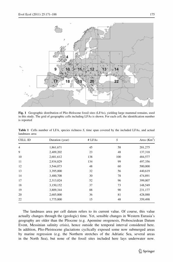
LFA geographic coordinates were imported in ArcGis 9.2 (ESRI) to produce a shapefile
recording their geographical distribution. As we dealt with a wide geographic area, we
used a Lambert Azimuthal Equal Area projection to avoid distortion of area due to the
variation of world’s curvature radius along meridians. We extracted a grid containing cells
of 500,000 Km2 (corresponding to squares of 707 km per side) from the LFA distribution
shapefile (Fig. 1), which minimizes the number of cells needed to include all LFAs. Then,
we calculated the actual landmass area within each cell of the grid (excluding the area
occupied by the sea, see Table 1) and counted the number of LFAs per cell.
174 Evol Ecol (2011) 25:171–188
123
The landmass area per cell datum refers to its current value. Of course, this value
actually changes through the (geologic) time. Yet, sensible changes in Western Eurasia’s
geography are older than the Pliocene (e.g. Apennine orogenesis, Probosciedean Datum
Event, Messinian salinity crisis), hence outside the temporal interval considered here.
In addition, Plio-Pleistocene glaciations cyclically exposed some now submerged areas
by marine regression (e.g. the Northern stretches of the Adriatic Sea, several areas
in the North Sea), but none of the fossil sites included here lays underwater now.
Fig. 1 Geographic distribution of Plio-Holocene fossil sites (LFAs), yielding large mammal remains, usedin this study. The grid of geographic cells including LFAs is shown. For each cell, the identification numberis reported
Table 1 Cells number of LFA, species richness S, time span covered by the included LFAs, and actuallandmass area
CELL ID Duration (year) # LFAs S Area (Km2)
4 1,861,671 45 58 201,275
9 2,409,202 23 48 137,318
10 2,681,612 138 100 484,577
11 2,934,829 134 99 497,356
12 3,544,073 48 60 500,000
13 3,395,000 32 56 440,619
14 3,400,708 30 78 474,891
17 2,313,024 52 96 399,007
18 3,150,152 37 73 148,549
19 3,809,344 88 90 231,177
20 2,685,000 36 81 428,088
22 1,775,000 15 48 359,498
Evol Ecol (2011) 25:171–188 175
123
Therefore, we consider that our estimation of cell surface area provides a good estimation of
the area occupied by the communities included in the analyses. Cells containing either less
than 7 LFAs, or whose LFAs cover a temporal interval less than 1.7 My long, were
excluded. We had empirically estimated that these criteria maximize the sample size
(=number of included cells) while maintaining high temporal coverage per cell. In total, 12
cells were retained and used as units of reference in order to produce SARs and STARs. As
our study is exploratory in essence, we avoided to define a priori specific biogeographical
provinces for which computing SAR (cfr. Barnosky et al. 2005). By using cells, we relied on
a restricted standardised criterion as for both the temporal and the spatial intervals to use.
STR, SAR and STAR calculation
We used three different statistical models of species accumulation (STR, SAR, and STAR)
representing two factors (time, space, and eventually their interaction) and all affected by
the same sampling noise (sampling inequality of LFAs over time and space). A first STR
model was fitted at the largest spatial scale (that is 12 selected geographical cells spanning
over the entire Western Eurasia subcontinent, see Fig. 1) by computing the increase in total
sampled species number (S) locality after locality, after LFAs had been collated in chro-
nologic order according to their numerical age estimates (see Appendix 1—Electronic
supplementary material). For each couple of consecutive LFAs (which are points in time)
we recorded cumulative S starting from the older LFA and the time span intervening
between the two. When two localities had the same age estimate, we took the cumulative
S value combining them as they were a single LFA. In this perspective, our species-time
curves resemble the computation of SAR across islands and our data points are ‘islands in
time’ (Hadly and Maurer 2001). We did not use the ‘‘moving window’’ (or complete-
nested, see Carey et al. 2007) approach that is familiar in most STR computations (White
2007) for it is inappropriate here (time-intervals between LFAs are irregular and some
LFAs have the same numerical age, therefore cannot be averaged). The STR is not devoid
of sampling problems, because the fossil record is obviously discontinuous, and younger
time intervals are represented by disproportionally more LFAs (Raia et al. 2006b, 2009).
To correct for this sampling inequality we computed a second STR as follows: we divided
our data set in 100 ky-long time bins. Thereby, 39 time bins were obtained, since the oldest
LFA is 3.73 My old. Then, we randomly selected one LFA per time bin and computed the
STR slope and log-likelihood. One-thousand random STRs were produced this way; the
average slope, and the maximum likelihood estimated slope were then computed and
compared to the w-exponent obtained by fitting a single STR to the entire database.
Besides problems in sampling inequality, the fossil record is plagued by taphonomic
biases. Preferential selection of some prey by predators, temporally and geographically
uneven effect of human hunting, differential conditions for preservation of, for instance,
large versus small specimens due to bone weathering and grain of the including sediments
are all relevant taphonomic factors. These factors may alter the distribution of species
abundances to some extent (but not dramatically, see Jernvall and Fortelius 2002; Raia
et al. 2006a) for instance by producing overrepresentation of some prey species or of larger
species (Damuth 1982). Yet, for STR or SAR computation either, it just matters whether a
given species is represented or not. The worst problem, then, could be the delay in the
(recorded) species first appearance event, which is true for any fossil record anyway, but
should not be particularly relevant with a fine-grained resolution as ours. By computing
STR and SAR this delay is not of an impact on the slope value (as it just produces a shift
along the 9 [time] axis), unless the delay in some (worse sampled) periods is larger than
176 Evol Ecol (2011) 25:171–188
123
in others. Since we have oversampling of younger faunas, the delay in species appearance
events should be lower for the latter, thereby increasing the calculated slope values. Yet, as
we decided to select only cells with similar duration, even this (hypothetical) issue, should
not be very problematic here.
The SAR model was similarly estimated by using all LFAs: we combined the cells into
random groups of 1, 2, 4, 8, and 12 cells, respectively, by exploring all possible combi-
nations of cells per group. For instance, with 12 cells there are 12 possible combinations of
group size = 1 cell, 66 possible combinations of group size = 2 cells, 495 possible
combinations of group size = 4 cells and so on. For each group, we computed a mean Sand a mean area, averaging over all possible combinations of cells. Logged S and area
averages were then regressed to each other. Our SAR sampling scheme is not nested, and
corresponds to type IIB curves in Scheiner (2003). In spite of the discussion about the
appropriateness of Scheiner’s classification to represent the differences between species-
area and species-accumulation curves (see Gray et al. 2004; Whittaker and Fernandez-
Palacios 2007), here we prefer to use it for the clarity of its definition in regard to the
accumulation processes we study. By taking the averages of all possible combinations we
could, at least partially, account for the uneven distribution of LFAs over time period and
over space (Raia et al. 2009).
Besides using all possible combinations of cells, we also computed SAR slopes by
extracting all the LFAs belonging to a single cell which are included in a given 500 ky-
long time interval. Data from consecutive time bins were then aggregated as to compute
the SAR. This procedure assumes that all the information available for each time bin is
limited to a single, randomly chosen, cell. One thousand SARs were produced this way.
The average z-exponent, and the maximum likelihood estimated z-exponent were then
computed.
There is strong evidence that the climatic signature (if any) on community evolution
differs between southern and northern faunas, in Europe (Rodrıguez 2006). To model these
possible differences, we calculated the median of the LFAs latitudes and partitioned the
record in two halves, one including LFAs staying north to the median (the ‘‘North’’
sample) the other including LFAs staying south to it (the ‘‘South’’ sample). SAR and STR
calculations, performed at different spatial and temporal scales, were repeated on the
‘‘North’’ and ‘‘South’’ subsets. We expect STR slopes should be steeper in the South,
because southern faunas hosted both typically warm-adapted taxa and cold-adapted taxa
(when glaciers advanced southwards because of cold phases), whereas Northern faunas
should typically include cold-adapted species only (Lister 2004). Hence, turnover ought to
be higher (in time) in the South. As of SAR slopes, we expect they are steeper in the South
because of possible regionalization of faunas distributed in the major South-European
peninsulas, and of reported homogeneity of Pleistocene high-latitude environments
(Guthrie 2001).
Finally, we computed the STAR model as in Adler and Lauenroth (2003) to estimate its
ability to predict richness at various combinations of temporal and spatial extents, and to
know how time and space interact with each other. Samplings over time were repeated at
increasing temporal intervals, from the oldest LFA to: 3 million years ago (3.0 My), 2.0,
1.0, 0.5, 0.1 and finally to 0.01 My. This means the first temporal interval includes all
LFAs older than 3 My, than the second includes all LFAs older than 2 My, the third
includes all LFAs older than 1 My and so on. For each temporal interval, spatial samplings
were repeated at spatial scales of 1, 2, 4, 8, and 12 cells (=all selected cells), respectively
(see Table 2). Since spatial scales of \12 cells comprehend a number of possible com-
binations of cells, we calculated a single S value per spatial scale by averaging across all
Evol Ecol (2011) 25:171–188 177
123
possible S (one for each combination of cells) as described above for the computation of
SAR. We assumed the minimum cell area and the minimum time span between successive
temporal sampling intervals as to represent the units of area and time, respectively. The
STAR model was then fitted to the data. A second STAR was calculated adding a fifth term
(the logarithm of the total number of LFAs at given space and time parameters) to the
equation, to correct for the unequal number of sites contributing to any given S value (for
instance, the number of LFAs per cell is highly correlated to its total species richness;
n = 12, r = 0.798; P = 0.002). This second STAR model takes the form:
log S ¼ log cþ z1 log Aþ w1 log T þ uðlog AÞðlog TÞ þ b log nLFAs
The coefficient u describes the degree of interaction (positive or negative, either)
between area and time.
A direct inspection of this interaction requires computing both SAR and STR exponents
at different temporal and spatial scales, respectively. If the interaction between area and
time on S is negative and linear, SAR exponent z must decline by sampling longer temporal
intervals, and STR exponent w must decline by sampling over larger spatial scale. For
SAR, we used the temporal intervals described above. As for STR, we calculated average
w obtained by testing all possible combinations of 1, 2, 4, 8, and 12 cells.
STR, SAR and STAR calculations at different scales were implemented in R.
Comparing STR slopes at different time periods
We tested the hypothesis that the STR slope changed in time, which is expected as a
consequence of the intense Quaternary cooling trend.
Five consecutive, non-nested STRs were produced using the temporal sampling points
described above as a reference. That is, one STR was computed over the 3.8–3 My
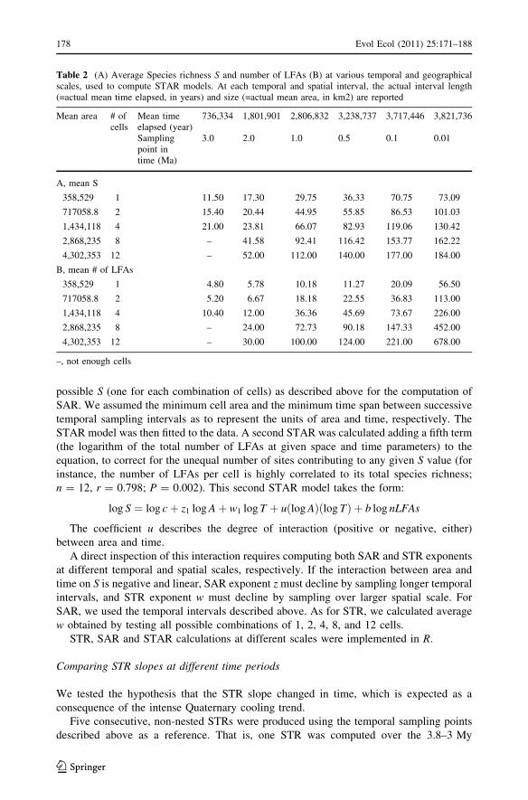
Table 2 (A) Average Species richness S and number of LFAs (B) at various temporal and geographicalscales, used to compute STAR models. At each temporal and spatial interval, the actual interval length(=actual mean time elapsed, in years) and size (=actual mean area, in km2) are reported
Mean area # ofcells
Mean timeelapsed (year)
736,334 1,801,901 2,806,832 3,238,737 3,717,446 3,821,736
Samplingpoint intime (Ma)
3.0 2.0 1.0 0.5 0.1 0.01
A, mean S
358,529 1 11.50 17.30 29.75 36.33 70.75 73.09
717058.8 2 15.40 20.44 44.95 55.85 86.53 101.03
1,434,118 4 21.00 23.81 66.07 82.93 119.06 130.42
2,868,235 8 – 41.58 92.41 116.42 153.77 162.22
4,302,353 12 – 52.00 112.00 140.00 177.00 184.00
B, mean # of LFAs
358,529 1 4.80 5.78 10.18 11.27 20.09 56.50
717058.8 2 5.20 6.67 18.18 22.55 36.83 113.00
1,434,118 4 10.40 12.00 36.36 45.69 73.67 226.00
2,868,235 8 – 24.00 72.73 90.18 147.33 452.00
4,302,353 12 – 30.00 100.00 124.00 221.00 678.00
–, not enough cells
178 Evol Ecol (2011) 25:171–188
123

interval, the second over the 3–2 My interval and so on. For these analyses, we decided to
exclude LFAs younger than 100 ky, in order to avoid biases that might be introduced by
either human activity (Pushkina and Raia 2008) or by the very high number of LFAs
younger than 100 ky in our dataset (Raia et al. 2009).
The STR w exponents are expected to be steeper in younger intervals (when climate
variability increased, White et al. 2006). Two statistical comparisons of w exponents were
computed. First, w differences were tested by ANCOVA. Then, all five STRs were forced
through the origin. Regression through the origin is theoretically permitted here because
when the increment in time sampled is 0 the increment in the number of species sampled
must be zero. Yet, residuals calculated by regressing through the origin do not sum to zero,
and the R-squared value cannot be directly compared to a model with the intercept. Since
ordinary least squares (OLS) regression is not advisable when forcing the model through
the origin because the error term is transferred to the dependent variable, we used stan-
dardized major axis (SMA) regression when STR models were fitted through the origin
(Keough and Quinn 2002). A fundamental property of regression through the origin is that
it ignores the intercept. In both SAR and STR the intercepts must be viewed as the species
richness at the unitary scales, but it is well known they influence the curvature (slope) of
the relationships as well (Rosenzweig 1995). Ignoring ‘‘standing’’ species richness is
particularly desirable here since this figure is greatly influenced by sampling intensity.
Since the latter is much greater in younger time intervals, we might have introduced a
systematic bias along the time axis by using regression models with intercepts. Therefore,
we decided to use regression through the origin as a complementary test for the difference
in w exponents, although we did not append any special significance to the exponents
themselves or to the R-squared values.
Results
Species richness per cell S varies in between 36 and 102 species (mean = 73.1; see
Table 1).
STR takes the form, S(T) = 2.48E-06 T1.190 (F = 16,243.4, nLFA = 677, R2 = 0.960,
P \ 0.001, 95% CI around the slope: 1.109–1.304, see Fig. 2a). SAR takes the form
S(A) = 0.70A0.337 (F = 126.7, n = 5, R2 = 0.992, P \ 0.001, 95% CI around the slope:
0.313–0.424, see Fig. 2b).
In both STAR models the z1 exponents we calculated (0.169 and 0.192) are much lower
than z obtained by fitting SAR (Table 3). The STAR scaling exponents w1 (1.00 and 0.680)
are similar to those reported by Rosenzweig (1998) for STRs calculated over the
Fig. 2 Species-time relationship plot (a). Specie-area relationship plot (b). The x-axis represents the log ofnumber of years sampled (a) and the log of the surface area sampled in Km2 (b). The y axis represents thelog of the number of species
Evol Ecol (2011) 25:171–188 179
123
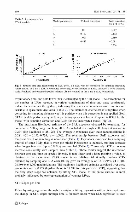
evolutionary time, and both lower than w calculated by the STR model. The corrections for
the number of LFAs recorded at various combinations of time and space consistently
reduce the w1 but not the z1 slope, indicating that species accumulation over time is more
sensible to space than vice versa (Table 2). The interaction coefficient u is negative when
correcting for sampling richness yet it is positive when this correction is not applied. Both
STAR models perform very well in predicting species richness, R square is 0.921 for the
model with sampling correction and 0.954 for the uncorrected model (Fig. 3).
The maximum likelihood estimate of the SAR exponent obtained by extracting, for
consecutive 500 ky long time bins, all LFAs included in a single cell chosen at random is
0.274 (log-likelihood = 28.125). The average z-exponents over these randomizations is
0.281 (CI = 0.192–0.734, n = 1,000). The relationship between SAR exponent and
temporal extent of sampling is non-linear (Table 4). Exponents z increase to a sampling
interval of some 3 My, that is when the middle Pleistocene is included, but then decrease
when longer intervals (up to 3.8 My) are sampled (Table 5). Conversely, STR exponents
increase consistently with sampled area (Table 4). These results suggest the interaction
between area and time on species diversity is non-linear, and a large positive u value, as
obtained in the uncorrected STAR model is not reliable. Additionally, random STRs
obtained by sampling one LFA each 100 ky gave an average w of 0.810 (95% CI 0.740–
0.879) over 1,000 randomizations. The maximum likelihood estimate calculated over these
randomizations is 0.777 (log-likelihood is 29.688 for this particular STR); suggesting that
the very steep slope we obtained by fitting STR model to the entire data-set is most
probably influenced by overrepresentation of younger LFAs.
STR slopes per time
Either by using regression through the origin or fitting regression with an intercept term,
the change in STR slopes through time is far from linear when OLS regression is used
Table 3 Parameters of theSTAR models
Model parameters Without correction With correctionfor # of LFAs
c 1.01 0.807
z1 0.169 0.192
w1 1.004 0.680
u 0.445 -0.091
b 0.334
Fig. 3 Species-time area relationship (STAR) plots. a STAR with no correction for sampling inequalityacross scales. In b the STAR is computed correcting for the number of LFAs included at each samplingscale. Predicted and observed species richness (S) are reported in the x and y axis, respectively
180 Evol Ecol (2011) 25:171–188
123

Ta
ble
4E
xp
on
ents
of
the
SA
Rm
od
elth
roug
hti
me
(z-
exp
onen
t)an
do
fth
eS
TR
mod
elth
rou
gh
spac
e(w
exp
on
ent)
To
tal
Tem
po
ral
sam
pli
ng
po
int
3.0
Ma
2.0
Ma
1.0
Ma
0.5
Ma
0.1
Ma
0.0
1M
a
z-E
xp
on
ent
0.4
75
(0.2
61–
0.7
46
)0
.344
(0.2
64–
0.4
32
)0
.620
(0.5
49–
0.7
05
)0
.683
(0.6
05
–0
.78
0)
0.4
71
(0.4
23
–0
.52
3)
0.3
67
(0.3
08
–0
.42
7)
Gro
up
size
(#o
fce
lls)
24
81
2
w-E
xp
on
ent
0.9
78
(0.1
60–
1.9
01
)1
.041
(0.6
30
–1
.45
4)
1.1
07
(0.8
03
–1
.34
5)
1.1
90
(1.1
09
–1
.30
4)
No
rth
z-E
xp
on
ent
0.5
64
a0
.274
a0
.618
(0.5
54–
0.6
83
)0
.675
(0.5
57
–0
.79
2)
0.4
11
(0.3
45
–0
.47
7)
0.3
63
(0.3
07
–0
.42
0)
w-E
xp
on
ent
0.8
33
(0.4
32–
1.9
91
)0
.924
(0.4
09
–2
.02
0)
0.8
84
(0.6
47
–1
.21
3)
0.8
18
(0.7
88
–0
.84
9)
So
uth
z-E
xp
on
ent
1.1
49
a0
.542
(0.4
20–
0.6
66
)0
.449
(0.3
50–
0.5
49
)0
.628
(0.5
06
–0
.74
9)
0.9
87
(0.8
03
–1
.16
8)
0.4
36
(0.3
49
–0
.52
4)
w-E
xp
on
ent
1.3
32
b
(0.1
55–
4.8
39
)1
.104
(0.1
30
–1
.86
5)
1.2
18
(1.1
62
–1
.26
8)
1.3
09
(1.2
62
–1
.35
6)
Co
nfi
den
cein
terv
als
are
rep
ort
edin
par
enth
eses
bel
ow
the
slop
es.
Fo
rb
oth
anal
yse
s,w
eca
lcu
late
dex
po
nen
tsb
yu
sin
gth
een
tire
reco
rd(t
ota
l);
and
then
repea
ted
the
anal
yse
so
nth
ere
cord
par
titi
on
edin
on
e‘‘
No
rth
’’an
do
ne
‘‘S
outh
’’h
alv
es,
repre
sen
tin
gL
FA
slo
cate
dei
ther
no
rthw
ard
or
sou
thw
ard
toth
eL
FA
sm
edia
nla
titu
de,
resp
ecti
vel
ya
Bas
edon
less
than
5ce
lls
bB
ased
on
two
com
bin
atio
ns
on
ly
Evol Ecol (2011) 25:171–188 181
123
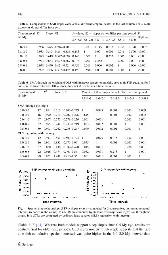
(Table 6; Fig. 4). Whereas both models support steep slopes since 0.5 My ago, results are
controversial for older time periods. OLS regression (with intercept) suggests that the rate
at which cumulative species increased was quite higher in the 3.0–2.0 My interval than
Table 5 Comparisons of SAR slopes calculated at different temporal scales. In the last column, H0 = SARexponents do not differ from zero
Time-interval(in My)
R2 Slope CI P-values, H0 = slopes do not differ per time period Pslope = 0
3.8–3.0 3.8–2.0 3.8–1.0 3.8–0.5 3.8–0.1 3.8–0
3.8–3.0 0.936 0.475 0.246–0.703 1 0.183 0.145 0.073 0.956 0.198 0.007
3.8–2.0 0.933 0.343 0.261–0.426 0.183 1 0.001 0.001 0.011 0.596 \0.001
3.8–1.0 0.973 0.619 0.542–0.697 0.145 0.001 1 0.252 0.006 0.001 \0.001
3.8–0.5 0.973 0.683 0.597–0.769 0.073 0.001 0.252 1 0.002 0.001 \0.001
3.8–0.1 0.978 0.470 0.421–0.52 0.956 0.011 0.006 0.002 1 0.006 \0.001
3.8–0 0.992 0.366 0.307–0.425 0.198 0.596 0.001 0.001 0.006 1 \0.001
Table 6 SMA through the origin and OLS with intercept regression models, used to fit STR equation for 5consecutive time intervals. H0 = slope does not differ between time periods
Time-interval(in My)
n R2 Slope CI P-values, H0 = slopes do not differ per time period
3.8–3.0 3.0–2.0 2.0–1.0 1.0–0.5 0.5–0.1
SMA through the origin
3.8–3.0 12 0.991 0.215 0.203–0.229 1 0.845 0.001 0.003 0.009
3.0–2.0 16 0.990 0.214 0.202–0.226 0.845 1 0.001 0.002 0.002
2.0–1.0 67 0.997 0.275 0.271–0.279 0.001 0.001 1 0.001 0.001
1.0–0.5 22 0.995 0.241 0.233–0.249 0.003 0.002 0.001 1 0.001
0.5–0.1 89 0.993 0.262 0.258–0.267 0.009 0.002 0.001 0.001 1
OLS regression with intercept
3.8–3.0 12 0.913 0.651 0.509–0.793 1 0.075 0.015 0.032 0.001
3.0–2.0 16 0.901 0.835 0.676–0.99 0.075 1 0.001 0.001 0.001
2.0–1.0 67 0.830 0.430 0.382–0.478 0.015 0.001 1 0.278 0.001
1.0–0.5 22 0.916 0.474 0.407–0.541 0.032 0.001 0.278 1 0.001
0.5–0.1 89 0.952 1.481 1.410–1.551 0.001 0.001 0.001 0.001 1
Fig. 4 Species-time relationships (STRs) slopes (y-axis) computed for 5 consecutive, not nested temporalintervals (reported in the x-axis). In a STRs are computed by standardized major axis regression through theorigin. In b STRs are computed by ordinary least squares (OLS) regression with intercept
182 Evol Ecol (2011) 25:171–188
123

in the succeeding 1 million year. Conversely, SMA regression (through the origin) indi-
cates that STR slopes were generally higher since 2 My (Table 6; Fig. 4).
Discussion
Species accumulation in time
Our STR slopes (both w and w1) are significantly higher than ever recorded in living
species (0.2–0.4 in Connor and McCoy 1979; and see Rosenzweig 1995, 1998). Yet,
according to Preston’s conjecture, models built on very large time intervals should show
steeper curves (Preston 1960; Rosenzweig 1995, 1998; McKinney and Frederick 1999;
Adler and Lauenroth 2003). This happens to be the case because over the evolutionary time
(our time span is as long as 3.8 My) speciation adds to the cumulative species richness
curve (which on the short-time ecological scale just depends on immigration of species
from surrounding areas). STR slope changes a little with sampling area (mean w changes
from 0.98 to 1.2 over a 12-fold increase in area, Table 4, and always with large confidence
intervals). The evidence that STR slope was not constant over time is robust (Table 6). Yet,
the notion that w increases linearly with time is controversial, depending on the regression
model applied. For older time periods, it is possible that the temporal spacing between
LFAs (which is definitely larger than for younger periods, see Appendix 1—Electronic
supplementary material) makes temporal turnover to appear more abrupt, and w to be
steeper as an artefact. If this is true, better sampling of younger time periods would produce
shallower slopes in these latter intervals. However, the increase in w over the past 500 ky is
supported by both regression methods and is probably genuine. Global climatic variability
became very intense during this period. For instance, mean annual surface temperatures in
Antartica were changing as much as 15�C from glacial to interglacial periods (Jouzel et al.
2007). The longest (and one of the warmest) interglacial, corresponding to Marine Isotopic
Stage (MIS) 11 occurs in this period (Raynaud et al. 2005), as does the coldest glacial
phase (MIS 2). The STR is an indirect proxy for temporal turnover (Rosenzweig 1998;
White 2004). As such, our results suggest that the pace of community evolution accelerated
during late Pleistocene. Elsewhere we got clear evidence that climatic changes controlled
temporal turnover, and that turnover rate peaked in the late Pleistocene (Raia et al. 2005;
Meloro et al. 2008). However, those studies were drawn at a much smaller spatial scale
(peninsular Italy vs Western Eurasia) than the present work. It is possible that the climatic
signature on faunal evolution in Italy is that evident for the latter behaved as a glacial
‘‘refugium’’ (Sommer and Zachos 2009), hosting continuous change in community com-
position, but not in ecological structure (Rodrıguez 2006), as the ice sheets retreated and
advanced in keeping with the glacial/interglacial cycles. This would indicate that the
chance of finding a climatic signature on community evolution is scale-dependent
(Barnosky 2001), and varies from place to place (Rodrıguez 2006). In keeping with this
contention, we found much higher STR slopes in southern, than in northern, faunas
(see Table 4).
Species accumulation over space
The SAR slopes are much closer to the values found for both living species and pale-
odiversity data computed within biogeographical provinces (that is in the 0.1–0.3 range,
Connor and McCoy 1979; Barnosky et al. 2005). Indeed, fitting a SAR model we got
Evol Ecol (2011) 25:171–188 183
123

an exponent of 0.34, yet this value is probably influenced by the large temporal scale
sampled, for both z1 exponents obtained by STAR models are much shallower. The
maximum likelihood estimate of z calculated by sampling one geographic cell per 500 ky
long time bin is 0.28, which is higher than z1s as well. Barnosky et al. (2005) obtained
shallower SAR slopes when paleodiversities were corrected for sampling bias by means of
rarefaction analysis. Yet, they did not account for the effect of time. Arguably, speciation,
immigration and climatic changes (and their interaction) have much less of an influence on
z than on w here for a number of reasons. Firstly, we analyzed mammal species whose
geographic ranges are much larger than Europe. Mammoths, horses, bison, aurochs, red
and fallow deer, roe deer, cave lion, leopard, wolf, cave hyena and cave bears occurred, to
name just a few renewed examples, over most of Asia, Africa, and even North America (in
a minority of cases). If this indicates climatic tolerance in these species, spatial turnover
could not have been very high anyhow. By restricting ourselves to large species we got
much larger ranges than for all mammals, hence much more similarity between local
faunas and shallower slopes than we would get by sampling smaller species as well.
Second, habitat heterogeneity is known to affect SAR slope (more diverse habitats have
higher spatial turnover, thereby produce higher SAR slopes, Kallimanis et al. 2008), but
there is evidence that habitat heterogeneity (in the geographical area we considered)
decreased during late Pleistocene. For instance, late Pleistocene environments in Northern
Europe were dominated by the so-called mammoth steppe, a homogeneous steppic biome
that extended from Western Eurasia to Kamchatka (Guthrie 2001). Not surprisingly, SAR
slopes calculated for Northern faunas appear much shallower during late Pleistocene times,
when the mammoth steppe was established (Table 4). In a similar vein, the high slopes in
the North we recorded for the 1–0.5 My time interval (Table 4) make sense when we
consider that during this time period it took place a massive immigration of new species
from Asia through Northern and Eastern Europe, thereby establishing what it is known as
the ‘‘Galerian’’ mammal age (Raia et al. 2009) in Europe. This immigration event is
recorded by SAR as well. When SAR is computed including the beginning of this period,
the z exponent becomes much steeper (Table 5). Thirdly, during the Ice Ages many species
are known to have moved repeatedly along a North-South vector in response to climatic
shifts (migrating southward when glaciers advanced in cold periods and vice versa during
more favorable climatic regimes, Lyons 2003; Lister 2004; Sommers and Zachos 2009). As
our SAR was computed over the whole continent, and over a temporal span including
several migratory events, shallow z are expected. Suppose, for example, to compute a SAR
counting species over an interval including both a glacial period and then an interglacial
phase. Now, consider a group of steppe (Northern) adapted species. These species will not
be counted in the South over a short phase in the interglacial, and not in the North during
the glacial. However, they will be counted in both the North and in the South over a longer
interval. If it was possible to compute SAR at a much shorter temporal intervals, we would
have got much steeper z. It is interesting to note, though, that SAR slopes computed for
older time periods are generally higher than for the late Pleistocene (Table 4). This sug-
gests higher regionalization of faunas during early and middle Pleistocene, at least at the
temporal resolution we used here. Although we could not dismiss this result to depend on
sampling inequality, it is in agreement with a previous study of ours (Raia et al. 2009)
indicating that there were at least two different and geographically disjunctive paleo-
communities in Western Eurasia throughout early to middle Pleistocene, but only one
distinct assemblage of species in younger (late Pleistocene) times.
184 Evol Ecol (2011) 25:171–188
123
Combining the effects of space and time
As for the estimation of diversity across scales, STAR models provide us with very good
estimates of cumulative species richness. The interaction factor u is negative in the STAR
model controlling for LFA richness (a measure of sampling intensity), which we argue
should be preferred over the uncorrected model. A negative interaction has been reported
for living species as well (Adler and Lauenroth 2003; Adler et al. 2005). This fact confirms
Preston’s second hypothesis (Preston 1960) that the rate of species accumulation over time
must decline as the sampled area increases and vice versa. The classic explanation for this
negative interaction is that at larger spatial scales a higher proportion of species in the
regional pool is identified over short time intervals, thereby reducing temporal species
accumulation rate (Adler and Lauenroth 2003; White 2004; White et al. 2006). This may
well be the case with Ice Age Western Eurasian large mammal faunas, which occurred in
two distinct paleocommunities during the Pliocene to middle Pleistocene period, and were
diachronous in the late Pleistocene because of massive and rapid intracontinental migration
along the North-South direction.
According to Vrba’s ‘‘turnover pulse’’ hypothesis, temporal taxonomic turnover is
buffered by (modest) habitat tracking and favours habitat specialization under ordinary
climatic oscillation, whereas more intense climate change disrupts community stability and
drives extinction and speciation events (Vrba 1995a, b). The first scenario should increase
SAR slopes, provided the calculation of SAR is framed at the proper scale. The second
scenario contributes to the increase in STR slopes. In keeping with these theoretical
expectations, we found z exponent was steeper during Pliocene to middle Pleistocene
times, when climate change was not as nearly intense as during the late Pleistocene, when
we record steeper w exponent.
Conclusion
Models built to describe species accumulation over space and over time at ecological
scales proved useful over the geologic time scale as well. Here, for Plio-Holocene large
mammals of Western Eurasia, we found that species accumulation rate over time was
much higher than over space, and was at least in part influenced by climatic changes. The
high w exponents we got are deemed to account for evolutionary phenomena not included
in STRs computed over the shorter –ecologic- temporal scale. This ‘‘third phase’’ of
species-time relationships show very high scaling exponents, as once found by Rosenzweig
(1998), although it is clear that the exponent itself is sensitive to the particular time period
considered for STR computation. There is evidence that space and time interact negatively
in determining species accumulation rates, in keeping with the findings of Adler and
Lauenroth (2003) and Adler et al. (2005). Consequently, particular attention to scale must
be given in any account of paleodiversity as already pointed out by Barnosky (2001) and
Barnosky et al. (2005).
Intra-continental dispersal is known to have been massive during the late Pleistocene.
Dispersal has probably increased community survival providing a limit to the influence of
climatic change effects at the continental scale. The greatly reduced opportunity for dis-
persal in modern faunas may prove very problematic for living species, in the light of
current climatic change.
Evol Ecol (2011) 25:171–188 185
123

Acknowledgments Shai Meiri and Anna Loy provided us with important comments and advice that let usincreasing the quality of this manuscript. Anastassios Kotsakis read an earlier version of the manuscript andhelped us collecting and preparing the database used for this study. We are grateful to two anonymousreviewers for their constructive comments on this manuscript.
References
Adler PB, Lauenroth WK (2003) The power of time: spatiotemporal scaling of species diversity. EcologyLett 6:749–756
Adler PB, White EP, Lauenroth WK, Kaufman DM, Rassweiler A, Rusak JA (2005) Evidence for a generalspecies-time-area relationship. Ecology 86:2032–2039
Alroy J (2000) New methods for quantifying macroevolutionary patterns and processes. Paleobiology26:707–733
Barnosky AD (2001) Distinguishing the effects of the Red Queen and Court Jester on Meiocene mammalevolution in the northern Rocky Mountains. J Vert Paleont 21:172–185
Barnosky AD, Kraatz BP (2007) The role of climatic change in the evolution of mammals. Bioscience57:523–532
Barnosky AD, Carrasco MA, Davis EB (2005) The impact of the species-area relationship on estimates ofpaleodiversity. Plos Biol 3:1356–1361
Bobe R, Behrensmeyer AK (2004) The expansion of grassland ecosystems in Africa in relation tomammalian evolution and the origin of the genus Homo. Palaeogeog Palaeoclimatol Palaeoecol207:399–420
Carey S, Ostling A, Harte J, del Moral R (2007) Impact of curve construction and community dynamics onthe species-time relationship. Ecology 88:2145–2153
Connor EF, McCoy ED (1979) The statistics and biology of the species-area relationship. Am Nat 113:791–833
Damuth J (1982) Analysis of the preservation of community structure in assemblages of fossil mammals.Paleobiology 8:434–446
Dengler J (2009) Which function describes the species-area relationship best? A review and empiricalevaluation. J Biogeog 36:728–744
Fattorini S (2007) To fit or not to fit? A poorly fitting procedure produces inconsistent results when thespecies—area relationship is used to locate hotspots. Biodiv Conserv 16:2531–2538
Fortelius M, Gionis A, Jernvall J, Mannila H (2006) Spectral ordering and biochronology of European fossilmammals. Paleobiology 32:206–214
Gray JS, Ugland KI, Lambshead J (2004) On species accumulation and species-area curves. Glob EcolBiogeogr 13:567–568
Guthrie RD (2001) Origin and causes of the mammoth steppe: a story of cloud cover, woolly mammal toothpits, buckles, and inside-out Beringia. Quat Sci Rev 20:549–574
Hadly EA, Maurer BA (2001) Spatial and temporal patterns of species diversity in montane mammalcommunities of western North America. Evol Ecol Res 3:477–486
Harte J, Kinzig A, Green J (1999) Self-similarity in the distribution and abundance of species. Science284:334–336
Hubbell SP (2001) The unified neutral theory of biodiversity and biogeography. Princeton University Press,Princeton
Jouzel J, Masson-Delmotte V, Cattani O, Dreyfus G, Falourd S, Hoffmann G, Minster B, Nouet J, BarnolaJM, Chappellaz J, Fischer H, Gallet JC, Johnsen S, Leuenberger M, Loulergue L, Luethi D, Oerter H,Parrenin F, Raisbeck G, Raynaud D, Schilt A, Schwander J, Selmo E, Souchez R, Spahni R, Stauffer B,Steffensen JP, Stenni B, Stocker TF, Tison JL, Werner M, Wolff EW (2007) Orbital and millennialAntarctic climate variability over the past 800,000 years. Science 317:793–796
Kallimanis AS, Mazaris AD, Tzanopoulos J, Halley JM, Pantis JD, Sgardelis SP (2008) How does habitatdiversity affect the species-area relationship? Global Ecol Biogeog 17:532–538
Keough MJ, Quinn GP (2002) Experimental design and data analysis for biologists 520 pages. CambridgeUniversity Press, Cambridge
Kinzig AP, Harte J (2000) Implications of endemics-area relationships for estimates of species extinctions.Ecology 81:3305–3311
Lister AM (2004) The impact of Quaternary Ice Ages on mammalian evolution. Phil Trans Roy Soc B359:221–241
Lyons SK (2003) A quantitative assessment of the range shifts of Pleistocene mammals. J Mammal 84:385–402
186 Evol Ecol (2011) 25:171–188
123
Lyons SK (2005) A quantitative model for assessing community dynamics of Pleistocene mammals. Am Nat165:E168–E185
Magurran AE (2007) Species abundance distributions over time. Ecology Lett 10:347–354May RM (1975) Patterns of species abundance and diversity. In: Diamond ML, Cody JM (eds) Ecology and
evolution of communities. Belknap Press, Cambridge, pp 81–120McKinney ML, Frederick DL (1999) Species-time curves and population extremes: Ecological patterns in
the fossil record. Evol Ecol Res 1:641–650Meloro C, Raia P, Carotenuto F, Barbera C (2008) Diversity and turnover of Plio-Pleistocene large mammal
fauna from the Italian Peninsula. Palaeogeog Palaeoclimat Palaeoecol 268:58–64Myers N, Mittermeier RA, Mittermeier CG, da Fonseca GAB, Kent J (2000) Biodiversity hotspots for
conservation priorities. Nature 403:853–858Pimm SL, Askins RA (1995) Forest losses predict bird extinctions in Eastern North-America. Proc Nat Acad
Sci USA 92:9343–9347Plotkin JB, Potts MD, Leslie N, Manokaran N, LaFrankie J, Ashton PS (2000) Species-area curves, spatial
aggregation, and habitat specialization in tropical forests. J Theor Biol 207:81–99Preston FW (1960) Time and space and variation of species. Ecology 41:611–627Pushkina D, Raia P (2008) Human influence on distribution and extinctions of the late Pleistocene Eurasian
megafauna. J Hum Evol 54:769–782Raia P, Piras P, Kotsakis T (2005) Turnover pulse or Red Queen? Evidence from the large mammal
communities during the Plio-Pleistocene of Italy. Palaeogeog Palaeoclimat Palaeoecol 221:293–312Raia P, Meloro C, Loy A, Barbera C (2006a) Species occupancy and its course in the past: macroecological
patterns in extinct communities. Evol Ecol Res 8:181–194Raia P, Piras P, Kotsakis T (2006b) Detection of Plio-Quaternary large mammal communities of Italy. An
integration of fossil faunas biochronology and similarity. Quat Sci Rev 25:846–854Raia P, Carotenuto F, Meloro C, Piras P, Barbera C, Kotsakis T (2009) More than three million years of
community evolution. The temporal and geographical resolution of the Plio-Pleistocene WesternEurasia mammal faunas. Palaeogeogr Palaeoclimat Palaeoecol 276:15–23
Raynaud D, Barnola JM, Souchez R, Lorrain R, Petit JR, Duval P, Lipenkov VY (2005) Palaeoclimatology:the record for marine isotopic stage 11. Nature 436:39–40
Rodrıguez J (2006) Structural continuity and multiple alternative stable states in Middle PleistoceneEuropean mammalian communities. Palaeogeog, Palaeoclim, Palaeoecol 239:355–373
Rodrıguez J, Alberdi MT, Azanza B, Prado JL (2004) Body size structure in north-western MediterraneanPlio-Pleistocene mammalian faunas. Global Ecol Biogeog 13:163–176
Rosenzweig ML (1995) Species diversity in space and time. Cambridge University Press, CambridgeRosenzweig ML (1998) Preston’s ergodic conjecture: the accumulation of species in space and time. In:
McKinney ML, Drake JA (eds) Biodiversity dynamics: turnover of populations, taxa, and communi-ties. Columbia University Press, New York, pp 311–348
Rosenzweig ML, Sandlin EA (1997) Species diversity and latitudes: listening to area’s signal. Oikos80:172–176
Scheiner SM (2003) Six types of species-area curves. Glob Ecol Biogeogr 12:441–447Shmida A, Wilson MV (1985) Biological determinants of species diversity. J Biogeog 12:1–20Sommer RS, Nadachowski A (2006) Glacial refugia of mammals in Europe: evidence from fossil records.
Mammal Rev 36:251–265Sommer RS, Zachos FE (2009) Fossil evidence and phylogeography of temperate species: ‘glacial refugia’
and post-glacial recolonization. J Biogeogr 36:2013–2020Triantis KA, Nogues-Bravo D, Hortal J, Borges PAV, Adsersen H, Fernandez-Palacios JM, Araujo MB,
Whittaker RJ (2008) Measurements of area and the (island) species-area relationship: new directionsfor an old pattern. Oikos 117:1555–1559
Turner WR, Tjørve E (2005) Scale-dependence in species—area relationships. Ecography 28:721–730Vrba ES (1995a) The fossil record of African antelopes (Mammalia, Bovidae) in relation to human evo-
lution and paleoclimate. In: Vrba ES, Denton GH, Partridge TC, Burckle LH (eds) Paleoclimate andevolution with emphasis on human origins. Yale University Press, New Haven, pp 385–424
Vrba ES (1995b) On the connections between paleoclimate and evolution. In: Vrba ES, Denton GH,Partridge TC, Burckle LH (eds) Paleoclimate and evolution with emphasis on human origins. YaleUniversity Press, New Haven, pp 24–48
White EP (2004) Two-phase species-time relationships in North American land birds. Ecology Lett 7:329–336
White EP (2007) Spatiotemporal scaling of species richness: patterns, processes, and implications. In: StorchD, Marquet PA, Brown JH (eds) Scaling biodiversity. Cambridge University Press, Cambridge,pp 325–346
Evol Ecol (2011) 25:171–188 187
123

White EP, Adler PB, Lauenroth WK, Gill RA, Greenberg D, Kaufman DM, Rassweiler A, Rusak JA, SmithMD, Steinbeck JR, Waide RB, Yao J (2006) A comparison of the species-time relationship acrossecosystems and taxonomic groups. Oikos 112:185–195
Whittaker RJ, Fernandez-Palacios JM (2007) Island biogeography. Ecology, evolution, and conservation,2nd edn. Oxford University Press, Oxford
Zachos J, Pagani M, Sloan L, Thomas E, Billups K (2001) Trends, rhythms, and aberrations in globalclimate 65 Ma to present. Science 292:686–693
188 Evol Ecol (2011) 25:171–188
123