Technical Report KDBSLAB-TR-94-04
Spatial Relations, Minimum Bounding Rectangles,and Spatial Data Structures
Dimitris Papadias
Department of Computer Science and EngineeringUniversity of California, San Diego
La Jolla, California, USA [email protected]
Yannis Theodoridis
Department of Electrical and Computer EngineeringNational Technical University of Athens
Zographou, Athens, GREECE [email protected]
Keywords: Topological and Direction relations, Spatial Data Structures,Minimum Bounding Rectangles, R-trees.
Acknowledgements: An early version of chapter 3 appears in (Papadias et al., 1994b), while chapters 4and 5 are based on (Papadias et al., 1994c). The ideas of this paper were refined by our collaboration withthe co-authors of these papers, namely, Timos Sellis and Max Egenhofer. Dimitris Papadias was partiallysupported by NSF - IRI 9221276. Yannis Theodoridis was partially supported by the Dept. of Researchand Technology of Greece (PENED 91).

Technical Report KDBSLAB-TR-94-04
Spatial Relations, Minimum Bounding Rectangles,and Spatial Data Structures
Abstract Despite the attention that spatial relations have attracted in domains such as
Spatial Query Languages, Image and Multimedia Databases, Reasoning and Geographic
Applications, they have not been extensively applied in spatial access methods. This
paper is concerned with the retrieval of topological and direction relations using spatial
data structures based on Minimum Bounding Rectangles. We describe topological and
direction relations between region objects and we study the spatial information that
Minimum Bounding Rectangles convey about the actual objects they enclose. Then we
apply the results in R-trees and their variations, R+-trees and R*-trees, in order to
minimise the number of disk accesses for queries involving topological and direction
relations. We also investigate queries that express complex spatial conditions in the form
of disjunctions and conjunctions, and we discuss possible extensions.
1
1. INTRODUCTION
The representation and processing of spatial relations is crucial in geographic applications because very
often in geographic space, relations among spatial entities are as important as the entities themselves.
Depending on the application domain, some spatial relations may be more significant than others:
topological relations have been used to access consistency in Geographical Databases (Egenhofer and
Sharma, 1993), ordinal relations to describe aggregation hierarchies (Kainz et al., 1993), and direction
relations have been incorporated in Spatial Query Languages (Papadias and Sellis, 1994a).
Topological relations describe concepts of neighbourhood, incidence and overlap and stay invariant
under transformations such as scaling and rotation. They are important for numerous practical
applications that involve queries of the form "find all land parcels adjacent to the main park". Our
approach on topological relations is based on the 4-intersection model (Egenhofer and Herring, 1990).
Tests with human subjects have shown evidence that this model, and its extension the 9-intersection
model (Egenhofer, 1991) have potential for defining cognitively meaningful spatial predicates, a fact that
renders them good candidates for commercial systems (Mark and Egenhofer, 1994). In fact, the 4- and 9-
intersection models have been implemented in Geographical Information Systems (GIS); Hadzilacos and
Tryfona (1992) used them to express geographical constraints, and Mark and Xia (1994) to determine
spatial relations in ARC/INFO. In addition there are implementations in commercial systems such as
Intergraph (MGE, 1993) and Oracle (Keighan, 1993).
Direction relations (north, north_east) deal with order in space. Unlike topological relations, there are
not widely accepted definitions of direction relations. Most people will agree that Germany is north of
Italy, but what about the relation between France and Italy? There are parts of France that are north of all
parts of Italy, but is it enough for stating that France is north of Italy?1 These concepts are directly
applicable to geographic applications where the formalization of spatial relations is crucial for user
interfaces and query optimisation strategies. Furthermore, the importance of direction relations has been
pointed out by several researchers in areas including Spatial Data Structures (Peuquet, 1986),
Geographic and Multimedia Databases (Papadias et al., 1994a, Sistla et al. 1994), Spatial Reasoning
(Glasgow and Papadias, 1992), Cognitive Science (Jackendoff, 1983) and Linguistics (Herskovits, 1986).
This paper shows how direction and topological relations between region objects can be processed in
Spatial Databases. Conventional Database Management Systems are designed to store one-dimensional
data (e.g., integers, records) and, as a result, the underlying data structures are not powerful enough to
efficiently handle boxes, polygons etc. On the other hand, the need to process multi-dimensional data in
applications, such as Cartography, Computer-Aided Design, and Computer Vision has led to the
1 A survey and an experimental study regarding the use of direction relations in cognitive spatial reasoning at geographicscales can be found in (Mark, 1992).
2
development of alternative spatial access methods. It is a common strategy in spatial access methods to
store object approximations and use these approximations to index the data space in order to efficiently
retrieve the potential objects that satisfy the result of a query. The paper is concerned with the retrieval of
objects that satisfy certain direction and topological relations using spatial methods based on Minimum
Bounding Rectangle (MBR) approximations. In particular we concentrate on R-trees and their variations.
Section 2 describes topological relations and Section 3 defines direction relations between extended
objects using definitions for points. Section 4 is concerned with MBRs and spatial data structures based
on them. Section 5 describes the retrieval of topological relations and Section 6 the retrieval of directions
relations using MBR-based data structures. Section 7 presents the tests in actual implementations and
compares the results. Section 8 discusses queries that involve both topological and direction information
and Section 9 concludes with comments about future work.
2. TOPOLOGICAL RELATIONS
The representation of topological relations is necessary for several practical applications that involve
neighbourhood, inclusion, overlap and related queries. In particular, in this section we describe
topological relations between region objects without holes as defined by the 4-intersection2 model
(Egenhofer and Herring, 1990). According to this model, each object p is represented in 2D space as a
point set which has an interior (denoted by po) and a boundary (denoted by ∂p). Let xi be a point (for the
rest of the paper points are denoted by a letter followed by a subscript). If we make the distinction
between the boundary and the interior, we can define the topological relation between two objects by
examining object intersections:¬ ∃ xi (xi ∈ ∂p ∧ xi ∈ ∂q) ∃ xi (xi ∈ ∂p ∧ xi ∈ ∂q)
¬ ∃ xj (xj ∈ po ∧ xj ∈ ∂q) ∃ xj (xj ∈ po ∧ xj ∈ ∂q)
¬ ∃ xk (xk ∈ ∂p ∧ xk ∈ qo) ∃ xk (xk ∈ ∂p ∧ xk ∈ qo)
¬ ∃ xl (xl ∈ po ∧ xl ∈ qo) ∃ xl (xl ∈ po ∧ xl ∈ qo)
The formulae in each line are pairwise disjoint; one is true, while the other is false for any pair of
objects. By taking conjunctions of four formulae, one from each line, we can create 16 pairwise disjoint
topological relations between objects. However not all of these relations are valid due to the constraints
imposed by the properties of the object boundaries and interiors. For instance, for all pairs of objects the
following constraints must always hold:
[∃ xl (xl ∈ po ∧ xl ∈ qo)] ⇒
[∃ xi (xi ∈ ∂p ∧ xi ∈ ∂q)∨ ∃ xj (xj ∈ po ∧ xj ∈ ∂q)∨ ∃ xk (xk ∈ ∂p ∧ xk ∈ qo)]
[¬ ∃ xl (xl ∈ po ∧ xl ∈ qo)∧ ¬ ∃ xi (xi ∈ ∂p ∧ xi ∈ ∂q)]⇒
2 Since we deal with region objects without holes, the 9 and 4 intersection models are equivalent in the sense that they permitthe same valid binary topological relations.

3
[¬ ∃ xj (xj ∈ po ∧ xj ∈ ∂q)∧ ¬ ∃ xk (xk ∈ ∂p ∧ xk ∈ qo)]
Out of the 16 possible relations that can be defined using the previous conjunctions only the following
eight illustrated in Table 1 are valid. These relations are proved to be pairwise disjoint, and they provide
a complete coverage (Randell et al., 1992). For each of the primitive relations Table 1 includes some
intersection points. The term primary object denotes the object to be located and the term reference
object denotes the object in relation to which the primary object is located. For the following examples
the primary objects are transparent and the reference objects are grey.
disjoint(p,q)
q
p
¬ ∃ xi (xi ∈ ∂p ∧ xi ∈ ∂q)∧ ¬ ∃ xj (xj∈ po ∧ xj∈ ∂q) ∧ ¬ ∃ xk (xk ∈ ∂p ∧ xk ∈ qo) ∧ ¬ ∃ xl (xl ∈ po ∧ xl ∈ qo)
meet(p,q)
qp
*xi
∃ xi (xi∈ ∂p ∧ xi ∈ ∂q) ∧ ¬ ∃ xj (xj ∈ po ∧ xj ∈ ∂q) ∧ ¬ ∃ xk (xk ∈ ∂p ∧ xk ∈ qo) ∧ ¬ ∃ xl (xl ∈ po ∧ xl ∈ qo)
overlap(p,q)
q p*
xi*
jx
*lx
*kx
∃ xi (xi ∈ ∂p ∧ xi ∈ ∂q) ∧ ∃ xj (xj ∈ po ∧ xj ∈ ∂q) ∧ ∃ xk (xk ∈ ∂p ∧ xk ∈ qo) ∧ ∃ xl (xl ∈ po ∧ xl ∈ qo)
covered_by(p,q)
qp
xi
**
lx*
kx
∃ xi (xi ∈ ∂p ∧ xi ∈ ∂q) ∧ ¬ ∃ xj (xj ∈ po ∧ xj ∈ ∂q) ∧ ∃ xk (xk ∈ ∂p ∧ xk ∈ qo) ∧ ∃ xl (xl ∈ po ∧ xl ∈ qo)
inside(p,q)
qp**
lx
kx
¬ ∃ xi (xi ∈ ∂p ∧ xi ∈ ∂q) ∧ ¬ ∃ xj (xj ∈ po ∧ xj ∈ ∂q) ∧ ∃ xk (xk ∈ ∂p ∧ xk ∈ qo) ∧ ∃ xl (xl ∈ po ∧ xl ∈ qo)
equal(p,q)
qp
xi**
lx
∃ xi (xi ∈ ∂p ∧ xi ∈ ∂q) ∧ ¬ ∃ xj (xj ∈ po ∧ xj ∈ ∂q) ∧ ¬ ∃ xk (xk ∈ ∂p ∧ xk ∈ qo) ∧ ∃ xl (xl ∈ po ∧ xl ∈ qo)

4
covers(p,q)
q
p
xi
*
*
lx
*jx
∃ xi (xi ∈ ∂p ∧ xi ∈ ∂q) ∧ ¬ ∃ xj (xj ∈ po ∧ xj ∈ ∂q) ∧ ∃ xk (xk ∈ ∂p ∧ xk ∈ qo) ∧ ∃ xl (xl ∈ po ∧ xl ∈ qo)
contains(p,q)
q
px
*l
*jx
¬ ∃ xi (xi ∈ ∂p ∧ xi ∈ ∂q) ∧ ∃ xj (xj ∈ po ∧ xj ∈ ∂q) ∧ ¬ ∃ xk (xk ∈ ∂p ∧ xk ∈ qo) ∧ ∃ xl (xl ∈ po ∧ xl ∈ qo)
Table 1 Topological relations
The disjunction of all topological relations that involve some non-empty intersection is called
not_disjoint, i.e., not_disjoint ≡ meet ∨ overlap ∨ covered_by ∨ inside ∨ equal ∨ covers ∨ contains. The
subset of topological relations that deal with the concepts of inclusion and containment have been called
ordinal or order relations (Kainz et al. 1993). Based on the above definitions we can define the following
ordinal relations:
− in(p,q) ≡ inside(p,q)∨ covered_by(p,q)
− consists_of(p,q) ≡ contains(p,q)∨ covers(p,q).
Topological (and ordinal) relations are very useful in geographic applications. The query “ find all
industrial areas of France adjacent to Italy” , for example, would require a search of industrial areas in
France that meet Italy. In the next section we discuss direction relations, another class of relations that are
important for practical applications.
3. DIRECTION RELATIONS
In order to define direction relations between extended objects we first define relations between points
and apply these definitions using universally and existentially quantified formulae. We assume an
absolute frame of reference and a pair of orthocanonic axes x and y. Our method is projection based, that
is, direction relations are defined using projection lines vertical to the coordinate axes. Another approach
is based on the cone-shaped concept of direction, i.e., direction relations are defined using angular
regions between objects. Extensive studies of the two approaches can be found in (Frank, 1994,
Hernandez, 1994).

5
Let pi be a point of object p (p denotes the primary object), qj be a point of object q (q denotes the
reference object), and X and Y be functions that return the x and y coordinate of a point. If we draw
projection lines from a reference point, the plane is divided into nine partitions (Figure 1)3.
X(q)
Y(q)
y
*
1
4
7
x
2 3
8
6
9
Fig. 1 Plane partitions using one point per object
Thus there are nine possible ways to put a primary point in the plane and therefore nine pairwise
disjoint relations that provide a complete coverage. These relations can be defined as:
north_west(pi,qj) ≡ X(pi)<X(qj) ∧ Y(pi)>Y(qj)
restricted_north(pi,qj) ≡ X(pi)=X(qj) ∧ Y(pi)>Y(qj)
north_east(pi,qj) ≡ X(pi)>X(qj) ∧ Y(pi)>Y(qj)
restricted_west(pi,qj) ≡ X(pi)<X(qj) ∧ Y(pi)=Y(qj)
same_position(pi,qj) ≡ X(pi)=X(qj) ∧ Y(pi)=Y(qj)
restricted_east(pi,qj) ≡ X(pi)>X(qj) ∧ Y(pi)=Y(qj)
south_west(pi,qj) ≡ X(pi)<X(qj) ∧ Y(pi)<Y(qj)
restricted_south(pi,qj) ≡ X(pi)=X(qj) ∧ Y(pi)<Y(qj)
south_east(pi,qj) ≡ X(pi)>X(qj) ∧ Y(pi)<Y(qj)
The above relations correspond to the highest accuracy that we can achieve when reasoning in terms
of points using the concept of projections, in the sense that they cannot be represented as disjunctions of
other relations. Exactly one of the previous relations holds true between any pair of points. The relations
are transitive and same_position is also symmetric. The rest form four pairs of converse relations (e.g.,
north_east(pi,qj) ⇔ south_west(qj, pi)). Additional direction relations can be defined using disjunctions of
the nine relations:
north(pi,qj) ≡ north_west(pi,qj) ∨ restricted_north(pi,qj) ∨ north_east(pi,qj)
east(pi,qj) ≡ north_east(pi,qj) ∨ restricted_east(pi,qj) ∨ south_east(pi,qj)
south(pi,qj) ≡ south_west(pi,qj) ∨ restricted_south(pi,qj) ∨ south_east(pi,qj)
west(pi,qj) ≡ north_west(pi,qj) ∨ restricted_west(pi,qj) ∨ south_west(pi,qj)
same_level(pi,qj) ≡ restricted_west(pi,qj) ∨ same_position(pi,qj) ∨ restricted_east(pi,qj)
same_width(pi,qj) ≡ restricted_north(pi,qj) ∨ same_position(pi,qj) ∨ restricted_south(pi,qj).
3 In general, if k is the number of points used to represent the reference object, then the plane is divided into (2k+1)2
partitions; k2 of the partitions are points, 2k(k+1) are open line segments and (k+1)2 are open regions. The numbers refer tothe case that none of the k points has a common co-ordinate with some other point.

6
Using the above definitions between points we define spatial relations between objects. The relation
strong_north between objects p and q denotes that all points of p are north of all points of q:
strong_north ≡ ∀ pi ∀ qj north(pi,qj). Figure 2a illustrates a configuration that corresponds to the relation
strong_north. As in the case of strong_north, all the relations between objects are defined using
universally and existentially quantified formulae representing relations between points. This is different
from (Papadias and Sellis, 1993; Papadias et al., 1994b) where direction relations are defined using
representative points. The relation weak_north can be defined as: weak_north(p,q) ≡ ∃ pi∀ qj north(pi,qj) ∧
∀ pi∃ qj north(pi,qj) ∧ ∃ pi∃ qj south(pi,qj). As Figure 2b illustrates, object p is weak_north of object q if:
− there exist some points of p which are north of all points of q (since ∃ pi∀ qj north(pi,qj)) and
− for each point pi there exist points qj such that north(pi,qj) (since ∀ pi∃ qj north(pi,qj)) and
− there exist some points of p which are south of some points of q (since ∃ pi∃ qj south(pi,qj)).
q
p
q
p
a b
Fig. 2 Strong_north and weak_north relation
The relation strong_bounded_north is defined as: strong_bounded_north(p,q) ≡ ∀ pi∀ qj north(pi, qj) ∧
∀ pi∃ qj north_east(pi, qj) ∧ ∀ pi ∃ qj north_west(pi, ql). According to Figure 3a, all points of object p must
be in the region bounded by the horizontal line that passes from q’s northmost point and by the vertical
lines that also bound q. In a similar manner we can define weak_bounded_north as,
weak_bounded_north(p,q) ≡ ∃ pi ∀ qj north(pi, qj) ∧ ∃ pi ∃ qj south(pi, qj) ∧ ∀ pi ∃ qj north_east(pi, qj) ∧ ∀ pi∃
qj north_west(pi, qj). As in the case of strong_bounded_north, object p is bounded by the vertical lines
that bound q, but p is also weak_north q (Figure 3.b).
q
p
q
p
a b
Fig. 3 Strong_bounded_north and weak_bounded_north relations
Strong_north_east is a variation of the strong_north relation which can be defined as
strong_north_east(p,q) ≡ ∀ pi ∀ qj north_east(pi, qj), i.e., all points of p must be north_east of all points of
q. Similarly we can define weak_north_east relation as: weak_north_east(p,q) ≡ ∃ pi∀ qj north_east(pi,qj) ∧

7
∃ pi∃ qjsouth(pi,qj) ∧ ∀ pi∃ qjnorth_east(pi,qj). Figure 4 illustrates strong_north_east and weak_north_east
relations.
q
p
q
p
a b
Fig. 4 Strong_north_east and weak_north_east relations
The relation just_north is defined as: just_north(p,q) ≡ ∀ pi ∀ qj (north(pi,qj) ∨ same_level(pi,qj)) ∧ ∃ pi
∃ qj same_level(pi,qj) ∧ ∃ pi ∃ qj north(pi,qj). As Figure 5a illustrates, according to this relation there must be
some point of p at the same_level with the northmost point of q, and all the other points of p must be
north of all points of q. We define the relation north between objects as: north(p,q) ≡ ∃ pi ∀ qj north(pi,qj)
∧ ∀ pi ∃ qj north(pi,qj), that is, there exist points of p that are north of all points of q, and for each point of
p there exist point(s) of q south of it (Figure 5b). It can be seen that north≡strong_north ∨ weak_north∨
just_north.
q
p
q
p
a b
Fig. 5 Just_north and north relations
All direction relations between objects that we have defined refer to the direction north. The relations
are not necessarily pairwise disjoint. In particular:
strong_north_east(p,q) ⇒ strong_north(p,q), strong_bounded_north(p,q) ⇒ strong_north(p,q),
weak_north_east(p,q) ⇒ weak_north(p,q), weak_bounded_north(p,q) ⇒ weak_north(p,q),
strong_north(p,q) ⇒ north(p,q),weak_north(p,q) ⇒ north(p,q), just_north(p,q) ⇒ north(p,q)
The definition of pairwise disjoint relations is not a difficult task, but it is beyond the scope of this
paper that aims to show how direction relations of different resolution between extended objects can be
defined and retrieved in spatial data structures. Furthermore since the above relations are concerned with
direction north only, they do not provide a complete coverage. Other directions can be formed in a
similar manner. Such relations are important because they allow the expression of queries in various
levels of qualitative resolution. As a special case consider the example with the direction relations of the
introduction and the map in Figure 6. According to the above definitions, France is weak_north, while
Germany is strong_north of Italy. Denmark is strong_bounded_north and Romania is weak_north_east
of Italy. All these variations of north may be very important for application domains where one concept

8
of “north” is not sufficient to express all configurations. Numerous additional relations between region,
line and point data can be defined and used in queries depending on the application needs. If we follow
the same terminology for the other directions, we can say that UK is strong_north_west and Spain is
strong_bounded_west of Italy
Fig. 6 A geographic example involving direction relations
Most of the work on direction relations has concentrated on point objects (Freksa, 1992; Frank, 1992).
According to this approach, each object is abstracted as one point, which may be the center of mass, the
center of symmetry etc. Our work extends previous approaches to direction relations by dealing with
extended objects instead of point objects. Peuquet and Ci-Xiang (1987) also designed an algorithm for
the determination of direction relations between arbitrary polygons represented by minimum bounding
rectangles. Unlike our approach, their method is based on the cone-shaped concept of direction and
involves only four direction relations (north, east, west and south).
4. MINIMUM BOUNDING RECTANGLES
Usually, spatial access methods instead of the actual objects, store approximations that need only a few
points for their representation. Such approximations are used to efficiently retrieve candidates that could
satisfy a query. Depending on the application domain there are several options in choosing object
approximations. Brinkhoff et al. (1993) compare the use of rotated minimum bounding rectangles,
convex hulls and minimum bounding n-corner convexes in spatial access methods. In this paper we
examine methods based on the traditional approximation of Minimum Bounding Rectangles. MBRs have
been used extensively to approximate objects in Spatial Data Structures and Spatial Reasoning because

9
they need only two points for their representation; in particular, each object q is represented as an ordered
pair (q'f,q's) of points that correspond to the lower left and the upper right point of the MBR q' that covers
q (q'f and q's are called the edge points - q'f stands for the first and q's for the second point of the MBR).
While MBRs demonstrate some disadvantages when approximating non convex or diagonal objects, they
are the most commonly used approximations in spatial applications. In the next subsection we investigate
the possible spatial relations between MBRs.
4.1 Spatial Relations between MBRs
When we use two points for the representation of the reference (region) object, the plane is divided into
25 partitions. Four partitions are points, 12 partitions are line segments and 9 partitions are open regions.
The character * in Figure 7a denotes the edge points of the reference MBR and the numbers correspond
to partitions. Therefore there are 25 ways to locate a primary point in the plane. If the primary object is
also represented by a pair of points ordered on the x and y axis (i.e., it is the MBR of a region object) the
number of possible relations between the two MBRs is 169. Figure 7b illustrates how the placement of
the first point of the primary object in a partition, constrains the number of possible partitions for the
second point. If for instance p'f is in partition 8 of Figure 7a, there are only three valid partitions for p's,
namely 3, 4 and 5. The sum of all numbers in Figure 7b is 169, that is, there are 169 unique placements
for the edge points and therefore 169 possible relations between MBRs (this number is the square of
possible relations between time intervals introduced in Allen 1983).
*Y(q's
*
1 2 3 4 56 7 8 10
11 12 13 15
16
14
18 19 20
21 22 23 24 25
Y(q' f
X(q'sX(q' f
)
)
) )
5 3 3 1 15 3 3 1
15 9 9 3
15
3
9 3 3
25 15 15 5 5
1
9
a b
Fig. 7 Plane partitions using two points per object
Figure 8 illustrates the possible configurations between MBRs. Each configuration corresponds to a
unique placement of points p'f and p's with respect to q'. R3-9, for instance, denotes that p'f is in partition
13 and p's in partition 3.

10
R i_1 R i_2 R i_3 R i_4 R i_5 R i_6 R i_7 R i_8 R i_9 R i_10 R i_11 R i_12 R i_13
R 1_j
R 2_j
R 3_j
R 4_j
R 5_j
R 6_j
R 7_j
R 8_j
R 9_j
R 10_j
R 11_j
R 12_j
R 13_j
Fig. 8 Possible relations between MBRs
Figure 9 illustrates the corresponding topological relation for the 169 configurations of Figure 8. For
instance, all the configurations of the first row (R1_j where j can take any value from 1 to 13) correspond
to the disjoint relation, and the total number of configurations in which the MBRs are disjoint is 48. On
the other hand, only relation R5_5 corresponds to the topological relation contains.
Disjoint 48
Meet 40
Overlap 50
Inside 1
Contains 1
CoveredBy 14
Covers 14
Equal 1
TOTAL 169
1 2 3 4 5 76 1098 11 12 13
1
2
3
4
5
7
6
10
9
8
11
12
13
Fig. 9 Topological relations between MBRs
The topological relation between MBRs yields useful information about the topological relation
between actual objects. If it is known that the MBRs are disjoint, it can be concluded that the objects they

11
enclose are also disjoint. Furthermore, depending on the relative positions of the edge points, several
conclusions can be drawn about the direction relationships between the actual objects, as for instance:
− north(p'f,q'f) ⇒ ∀ pi ∃ qj north(pi,qj),
− north(p'f,q's) ⇒ ∀ pi ∀ qj north(pi,qj),
− north(p's,q'f) ⇒ ∃ pi ∃ qj north(pi,qj) and
− north(p's,q's) ⇒ ∃ pi ∀ qj north(pi,qj).
For example, north(p'f,q's) implies that all points of object p are north of all points of object q. This
relation between p and q was call called strong_north in Section 3. In Figure 8, strong_north is mapped
onto relations R1-j where j can take any value from 1 to 13 because these relations correspond to the only
configurations in which north(p'f,q's). Therefore, the result of the query “ find all objects strong_north of
object q” consists of all objects whose MBRs satisfy the relation R1-j. In sections 5 and 6 we discuss in
detail the topological and direction information that MBRs convey about the actual objects they enclose
and how this information can be used for query optimisation techniques in MBR-based data structures.
4. 2 Spatial Data Structures based on MBRs
The most promising group of spatial data structures based on MBRs includes R-trees (Guttman, 1984)
and their variations. The R-tree data structure is a height-balanced tree, which consists of intermediate
and leaf nodes (R-trees are direct extensions of B-trees in k-dimensions). The MBRs of the actual data
objects are assumed to be stored in the leaf nodes of the tree. Intermediate nodes are built by grouping
rectangles at the lower level. An intermediate node is associated with some rectangle which encloses all
rectangles that correspond to lower level nodes. Each pair of nodes may satisfy any of the 169
configurations of Figure 8. Figure 10 shows how the map of Figure 6 is represented by MBRs and stored
in an R-tree. We assume a branching factor of 4, i.e., each intermediate node contains at most four
entries. At the lower level MBRs of countries (denoted by two letters) are grouped into five intermediate
nodes A, B, C, D and E. At the next level, the five nodes are grouped into two larger nodes X and Y.
Figure 10b illustrates the corresponding R-tree.
GRIT
SP
PO
FR
IR
UK
DE
GE
NL
BE
PL
CH
RO
BU
AL
YU
AU
CZ
HU
A
B
C
D
E
X
Y A B E
PO SP FR BE IR UK NL DE GE CH AU
X Y
IT
D C
GR YU AL BU RO HU CZ PL
a b
Fig. 10 Some MBRs grouped into intermediate rectangles and the corresponding R-tree

12
The fact that R-trees permit overlap among node entries sometimes leads to unsuccessful hits on the
tree structure. The R+-tree (Sellis et al., 1987) and the R*-tree (Beckmann et al., 1990) methods have
been proposed to address the problem of performance degradation caused by the overlapping regions or
excessive dead-space respectively. To avoid this problem, R+-tree achieves zero overlap among
intermediate node entries by allowing partitions to split nodes. The trade-off is that more space is
required because of the duplicate entries and thus the height of the tree may be greater than the original
R-tree. On the other hand, the R*-tree permits overlap among nodes, but tries to minimise it by
organising rectangles into nodes using a more complex algorithm than the one of the original R-tree.
Figure 11 illustrates how each method would organise a set of rectangles into intermediate nodes. The
original R-tree would create two intermediate nodes A and B. Node A contains MBRs 1,2,3 and 6 (the
grey MBRs) and node B contains 7, 4 and 5 (Figure 11a). The R+-tree algorithm splits rectangles that fall
on some partition line (rectangles 2 and 7) achieving zero overlap between A and B. This results in
duplicate entries that may increase the number of intermediate nodes (if we assume a branching factor of
4 we have an extra node C) (Figure 11b). The R*-tree algorithm groups rectangles in a different way in
order to achieve smaller overlap and coverage area of the intermediate nodes compared to the original R-
tree algorithm (Figure 11c).
1
2
7
6 4
3
5
A B
1
2
7
6 4
3
5
A
B
7
2
C
1
2
7
6 4
3
5
A B
c b c
Fig. 11 Some rectangles and the corresponding grouping in the R-tree variants
So far, R trees and their variations have been used for queries involving only the relations disjoint and
not_disjoint. If these are the only relations of interest, then when the MBRs of two objects are disjoint we
can conclude that the objects that they represent are also disjoint. If the MBRs however share common
points, no conclusion can be drawn about the spatial relation between the objects (they can be disjoint or
not_disjoint). For this reason, spatial queries involve the following two step strategy:
1. Filter step: The tree is used to rapidly eliminate objects that could not possibly satisfy the query. The
result of this step is a set of candidates which includes all the results and possibly some false hits.
2. Refinement step: Each candidate is examined (by using computational geometry techniques). False
hits are detected and eliminated.
Brinkhoff et al. (1993b) extended the above strategy to include a second filter step with finer
approximations than MBR (e.g. convex hulls) in order to exclude some false hits from the set of
candidates. The present work uses the original two-step strategy to explore a larger, and more detailed set
of direction and topological relations. Such an investigation is important because spatial queries

13
frequently require the kind of qualitative resolution distinguished by the topological and direction
relations of sections 2 and 3.
5. IMPLEMENTATION OF TOPOLOGICAL RELATIONS
Since the MBRs are only approximations of the actual objects, the topological relation between MBRs
does not necessarily coincide with the topological relation between the objects. In order to answer the
query "find all objects p equal to object q" we need to retrieve all MBRs that are equal with q', because
only they may enclose objects that satisfy the query. According to Figure 9 these MBRs satisfy the
relation R7-7 with respect to q'. On the other hand, the retrieved MBRs may enclose objects that satisfy
the relations equal, overlap, covered_by, covers or meet with respect to q (see Figure 12). A refinement
step is needed when dealing with topological relations, if the MBRs of the retrieved objects are not
disjoint.
q
pq
pqp
qp
q
p
Fig. 12 Possible relations for objects when the MBRs are equal
The relations contains and inside also involve the retrieval of MBRs that satisfy unique
configurations. In particular, the objects that contain q can only be in MBRs that contain q' (MBRs that
satisfy the relation R5-5 with respect to q'), while the objects inside q, can only be in MBRs that are inside
q' (MBRs that satisfy the relation R9-9 with respect to q'). As in the case of equal, a refinement step is
needed because:
− contains(p',q') ⇒ disjoint(p,q)∨ meet(p,q)∨ overlap(p,q)∨ contains(p,q)∨ covers(p,q) and
− inside(p',q') ⇒ disjoint(p,q)∨ meet(p,q)∨ overlap(p,q)∨ inside(p,q) ∨ covered_by(p,q)
The rest of the relations involve the retrieval of more than one MBR configurations. In case of covers,
all MBRs that satisfy the relations Ri-j where i and j in {4,5,7,8} with respect to q' should be retrieved
(MBRs that satisfy the relations covers, contains, equal with respect to q'). As Figure 13 illustrates, these
MBRs may enclose objects that cover the reference object. Similarly the retrieval of covered_by involves
all MBRs that satisfy the relations Ri-j where i,j in {6,7,9,10} with respect to q' (MBRs that satisfy the
relations covered_by, inside, equal). The remaining relations involve the retrieval of a large number of
MBRs. In the case of disjoint, for instance, all the MBRs may enclose objects that are disjoint with the
reference object.

14
R i_4 R i_5 R i_7 R i_8
R 4_j
R 5_j
R 7_j
R 8_j
Fig. 13 Configurations of MBRs that yield the relation covers between actual objects
We followed the same procedure for the relations meet and overlap. Table 2 shows the conclusions
that can be drawn if we use the concept of projections to study topological relations. The first column of
Table 2 contains the topological relation for the actual objects and the second column a configuration that
satisfies the relation. The third column describes the corresponding relation(s) between MBRs and the
fourth column illustrates the subset of the 169 configurations that satisfy this relation (the grey
configurations are to be retrieved for the query “retrieve all objects that satisfy the relation of the first
column”). The table refers to contiguous or non-contiguous region objects. If we assume contiguity we
can restrict the output MBRs for some relations (Papadias et al., 1994c).
Topological relationbetween actual objects
p and q
Illustration Leaf nodes p' to be retrieved Illustration of the correspondingprojections
equal(p,q)q
p
equal(p',q') 1 2 3 4 5 76 1098 11 12 13
1
2
3
4
5
7
6
10
9
8
11
12
13
contains(p,q)
q
p
contains(p',q') 1 2 3 4 5 76 1098 11 12 13
1
2
3
4
5
7
6
10
9
8
11
12
13

15
inside(p,q)
qp
inside(p',q') 1 2 3 4 5 76 1098 11 12 13
1
2
3
4
5
7
6
10
9
8
11
12
13
covers(p,q)
q
p covers(p',q') ∨ contains(p',q') ∨equal(p',q')
1 2 3 4 5 76 1098 11 12 13
1
2
3
4
5
7
6
10
9
8
11
12
13
covered_by(p,q)
qp
covered_by(p',q') ∨ inside(p',q')∨ equal(p',q')
1 2 3 4 5 76 1098 11 12 13
1
2
3
4
5
7
6
10
9
8
11
12
13
disjoint(p,q)
q
p disjoint(p',q') ∨ meet(p',q') ∨overlap(p',q') ∨ covered_by(p',q')
∨ inside(p',q') ∨ equal(p',q') ∨covers(p',q') ∨ contains(p',q')
1 2 3 4 5 76 1098 11 12 13
1
2
3
4
5
7
6
10
9
8
11
12
13
meet(p,q)
qp
meet(p',q') ∨ overlap(p',q') ∨covered_by(p',q') ∨ inside(p',q') ∨
equal(p',q') ∨ covers(p',q') ∨contains(p',q')
1 2 3 4 5 76 1098 11 12 13
1
2
3
4
5
7
6
10
9
8
11
12
13
overlap(p,q)q p
overlap(p',q') ∨ covered_by(p',q') ∨ inside(p',q') ∨ equal(p',q') ∨covers(p',q') ∨ contains(p',q')
1 2 3 4 5 76 1098 11 12 13
1
2
3
4
5
7
6
10
9
8
11
12
13
Table 2 MBRs to be retrieved for topological relations

16
The above mapping from topological relations between actual objects to relations between MBRs
refers to leaf nodes. In order to retrieve topological relations using R-trees one needs to define more
general relations that will be used for propagation in the intermediate nodes of the tree structure. For
instance, the intermediate nodes P that could enclose MBRs p' that meet the MBR q' of the reference
object q, should satisfy the more general constraint meet(P,q') ∨ overlap(P,q') ∨ covers(P,q') ∨
contains(P,q'). Figure 14 illustrates examples of such configurations.
P
p'
q'
P
p'
q'
P
p'
q'
P
p'
q'
a b c d
Fig. 14 Intermediate nodes that may contain MBRs that meet the MBR of the reference object
In our geographic example, if we want to find the countries that meet Switzerland, we can directly
exclude all countries in intermediate node Y because they are disjoint with the MBR CH of Switzerland.
Similarly sub-node B is excluded while nodes A and E are selected for propagation. The output MBRs of
the search are IT, AU, GE and FR because they overlap with CH and therefore the actual objects may
meet according to Table 2. The grey MBRs in Figure 15a correspond to potential candidates for the
query, while the grey nodes of Figure 15b are the ones that satisfy the search conditions.
GRIT
SP
PO
FR
IR
UK
DE
GE
NL
BE
PL
CH
RO
BU
AL
YU
AU
CZ
HU
A
B
C
D
E
X
Y
GE CH AU IT
A B
PO SP BE IR UK NL DE
D
GR YU AL BU RO HU CZ PL
X
E
Y
C
FR
a b
Fig. 15 An example search for topological queries
Following this strategy, the search space is pruned by excluding the intermediate nodes P that do not
satisfy the previous constraint. Table 3 presents the relations that should be satisfied between an
intermediate node P and the MBR q' of the reference object, so that the node will be selected for
propagation.
17
Relation betweenMBRs p' and q'
Relation between intermediate node P (that may enclose MBRs p')and reference MBR q'
equal(p',q') equal(P,q') ∨ covers(P,q') ∨ contains(P,q')
contains(p',q') contains(P,q')
inside(p',q') overlap(P,q') ∨ covered_by(P,q') ∨ inside(P,q') ∨ equal(P,q') ∨ covers(P,q') ∨ contains(P,q')
covers(p',q') covers(P,q') ∨ contains(P,q')
covered_by(p',q') overlap(P,q') ∨ covered_by(P,q') ∨ equal(P,q') ∨ covers(P,q') ∨ contains(P,q')
disjoint(p',q') disjoint(P,q') ∨ meet(P,q') ∨ overlap(P,q') ∨ covers(P,q') ∨ contains(P,q')
meet(p',q') meet(P,q') ∨ overlap(P,q') ∨ covers(P,q') ∨ contains(P,q')
overlap(p',q') overlap(P,q') ∨ covers(P,q') ∨ contains(P,q')
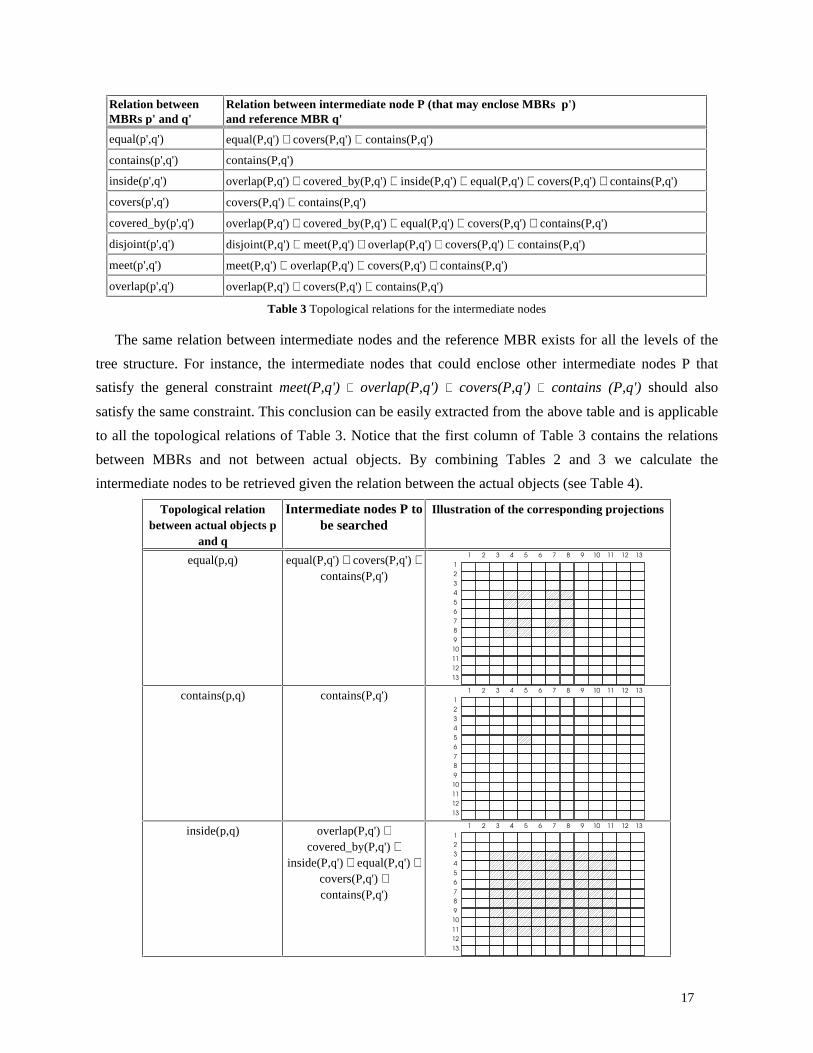
Table 3 Topological relations for the intermediate nodes
The same relation between intermediate nodes and the reference MBR exists for all the levels of the
tree structure. For instance, the intermediate nodes that could enclose other intermediate nodes P that
satisfy the general constraint meet(P,q') ∨ overlap(P,q') ∨ covers(P,q') ∨ contains (P,q') should also
satisfy the same constraint. This conclusion can be easily extracted from the above table and is applicable
to all the topological relations of Table 3. Notice that the first column of Table 3 contains the relations
between MBRs and not between actual objects. By combining Tables 2 and 3 we calculate the
intermediate nodes to be retrieved given the relation between the actual objects (see Table 4).
Topological relationbetween actual objects p
and q
Intermediate nodes P tobe searched
Illustration of the corresponding projections
equal(p,q) equal(P,q') ∨ covers(P,q') ∨contains(P,q')
1 2 3 4 5 76 1098 11 12 13
1
2
3
4
5
7
6
10
9
8
11
12
13
contains(p,q) contains(P,q') 1 2 3 4 5 76 1098 11 12 13
1
2
3
4
5
7
6
10
9
8
11
12
13
inside(p,q) overlap(P,q') ∨covered_by(P,q') ∨
inside(P,q') ∨ equal(P,q') ∨covers(P,q') ∨contains(P,q')
1 2 3 4 5 76 1098 11 12 13
1
2
3
4
5
7
6
10
9
8
11
12
13

18
covers(p,q) equal(P,q') ∨ covers(P,q') ∨contains(P,q')
1 2 3 4 5 76 1098 11 12 13
1
2
3
4
5
7
6
10
9
8
11
12
13
covered_by(p,q) overlap(P,q') ∨covered_by(P,q') ∨
inside(P,q') ∨ equal(P,q') ∨covers(P,q') ∨contains(P,q')
1 2 3 4 5 76 1098 11 12 13
1
2
3
4
5
7
6
10
9
8
11
12
13
disjoint(p,q) disjoint(P,q') ∨ meet(P,q') ∨overlap(P,q') ∨
covered_by(P,q') ∨inside(P,q') ∨ equal(P,q') ∨
covers(P,q') ∨contains(P,q')
1 2 3 4 5 76 1098 11 12 13
1
2
3
4
5
7
6
10
9
8
11
12
13
meet(p,q) meet(P,q') ∨ overlap(P,q') ∨covered_by(P,q') ∨
inside(P,q') ∨ equal(P,q') ∨covers(P,q') ∨contains(P,q')
1 2 3 4 5 76 1098 11 12 13
1
2
3
4
5
7
6
10
9
8
11
12
13
overlap(p,q) overlap(P,q') ∨covered_by(P,q') ∨
inside(P,q') ∨ equal(P,q') ∨covers(P,q') ∨contains(P,q')
1 2 3 4 5 76 1098 11 12 13
1
2
3
4
5
7
6
10
9
8
11
12
13
Table 4 General relations for the intermediate nodes
The ordinal relations defined in Section 2 can also be processed by the above method. Consider the
query "find all land parcels in a given area". The land parcels of the result should be inside or should be
covered_by the area, because the interpretation of in is inside ∨ covered_by. The set of the MBRs to be
retrieved in this case is the union of the MBRs to be retrieved by each of the relations that belong to the
disjunction. Furthermore, the MBRs of the result are the same ones that would be retrieved if the relation
of interest were covered_by. This is because the MBRs to be retrieved for inside constitute a subset of the

19
MBRs for covered_by (see Table 2). Similarly the MBRs to be retrieved for consists_of are the ones that
are retrieved for cover. Therefore, the retrieval times for the ordinal relations in and consists_of are the
same as covered_by and covers respectively.
Clementini et al. (1994) studied the use of MBR approximations in query processing involving
topological relations. Furthermore, they defined a minimal subset of the nine intersections that can
optimally determine the relation between the actual objects taking in account the frequency of the
relations. Their findings can be used during the retrieval step in order to minimise the cost for the
computation of intersections between potential candidates.
6. IMPLEMENTATION OF DIRECTION RELATIONS
As in the case of topological directions, for directions we need to define a mapping function that maps
relations between actual objects onto relations between MBRs. In section 4, we mentioned, for example,
that the relation strong_north is mapped onto the 13 configurations of the first row of Figure 8. Unlike
strong_north, which is mapped onto a set of MBR configurations, other direction relations are mapped
onto unique relations. Weak_bounded_north, for instance, is mapped onto relation R3-9, that is, objects
weak_bounded_north of a reference object q can only be in MBRs that satisfy the relation R3-9 with
respect to q'.
Table 5 illustrates the mappings from direction relations between actual objects to MBR relations. The
first column contains the eight direction relations of Section 3 and the second column illustrates a
configuration of objects that satisfies the relation. The third column describes the corresponding relations
between MBRs using relations between the edge points. The last column illustrates the MBRs of the
third column graphically.
Relation betweenactual objects p and q
Illustration Leaf nodes p' to be retrieved Illustration of the correspondingprojections
strong_north(p,q)
q
p north(p'f,q's)1 2 3 4 5 76 1098 11 12 13
1
2
3
4
5
7
6
10
9
8
11
12
13
weak_north(p,q)
q
p north(p's,q's) ∧ north(p'f,q'f) ∧south(p'f,q's)
1 2 3 4 5 76 1098 11 12 13
1
2
3
4
5
7
6
10
9
8
11
12
13

20
strong_bounded_north(p,q)
q
p north(p'f,q's) ∧north_east(p'f,q'f) ∧north_west(p's,q's)
1 2 3 4 5 76 1098 11 12 13
1
2
3
4
5
7
6
10
9
8
11
12
13
weak_bounded_north(p,q)
q
p
south(p'f,q's) ∧north_east(p'f,q'f) ∧north_west(p's, q's)
1 2 3 4 5 76 1098 11 12 13
1
2
3
4
5
7
6
10
9
8
11
12
13
strong_north_east(p,q)
q
p north_east(p'f,q's)1 2 3 4 5 76 1098 11 12 13
1
2
3
4
5
7
6
10
9
8
11
12
13
weak_north_east(p,q)
q
p
north_east(p's,q's)∧north_east(p'f,q'f) ∧
south(p'f,q's)
1 2 3 4 5 76 1098 11 12 13
1
2
3
4
5
7
6
10
9
8
11
12
13
just_north(p,q)
q
p same_level(p'f,q's)1 2 3 4 5 76 1098 11 12 13
1
2
3
4
5
7
6
10
9
8
11
12
13
north(p,q)
q
p north(p'f,q'f) ∧ north(p's,q's)1 2 3 4 5 76 1098 11 12 13
1
2
3
4
5
7
6
10
9
8
11
12
13
Table 5 MBRs to be retrieved for direction relations
Similar to topological relations, to retrieve direction relations using R-trees one needs to define more
general relations that will be used for propagation in the intermediate nodes of the tree structure. For

21
instance, to find all countries p strong_north_east of Switzerland we need to retrieve all the MBRs p'
within the leaf nodes that satisfy the constraint north_east(p'f,CHs), that is, the MBRs in the grey area of
Figure 16a. However, the intermediate nodes P that could contain such MBRs should satisfy the
constraint north_east(Ps, CHs). In the R-tree of Figure 16b, intermediate nodes X and Y may both contain
candidate MBRs and are selected for propagation. In node Y, only intermediate node C satisfies the
constraint north_east(Cs,CHs) and is searched, while the remaining nodes are directly excluded (C
contains the only objects that satisfy the query, namely CZ and PL). Similarly, the searched sub-nodes of
X are B and E.
GRIT
SP
PO
FR
IR
UK
DE
GE
NL
BE
PL
CH
RO
BU
AL
YU
AU
CZ
HU
A
B
C
D
E
X
Y A B
PO SP FR BE IR UK NL DE GE CH AU IT
D
GR YU AL BU RO HU CZ PL
X
E
Y
C
a b
Fig. 16 An example search for direction queries
Table 6 describes the direction constraint for the intermediate nodes and the corresponding
configurations to be searched for each direction relation between actual objects.
Relation betweenactual objects p and q
Intermediate nodes P to besearched
Illustration of the correspondingprojections
strong_north(p,q) north(Ps,q's)1 2 3 4 5 76 1098 11 12 13
1
2
3
4
5
7
6
10
9
8
11
12
13
weak_north(p,q) north(Ps,q's)∧ south(Pf,q's)1 2 3 4 5 76 1098 11 12 13
1
2
3
4
5
7
6
10
9
8
11
12
13

22
strong_bounded_north(p,q)
north(Ps,q's) ∧ west(Pf,q's) ∧east(Ps,q'f)
1 2 3 4 5 76 1098 11 12 13
1
2
3
4
5
7
6
10
9
8
11
12
13
weak_bounded_north(p,q)
north(Ps,q's) ∧ south(Pf,q's) ∧west(Pf,q's) ∧
east(Ps,q'f)
1 2 3 4 5 76 1098 11 12 13
1
2
3
4
5
7
6
10
9
8
11
12
13
strong_north_east(p,q) north(Ps,q's) ∧east(Ps,q's)
1 2 3 4 5 76 1098 11 12 13
1
2
3
4
5
7
6
10
9
8
11
12
13
weak_north_east(p,q) north(Ps,q's) ∧ south(Pf,q's) ∧ east(Ps,q's)
1 2 3 4 5 76 1098 11 12 13
1
2
3
4
5
7
6
10
9
8
11
12
13
just_north(p,q) (north(Ps, q's) ∧ ((south(Pf, q's) ∨same_level(Pf, q's) )
1 2 3 4 5 76 1098 11 12 13
1
2
3
4
5
7
6
10
9
8
11
12
13
north(p,q) north(Ps,q's)1 2 3 4 5 76 1098 11 12 13
1
2
3
4
5
7
6
10
9
8
11
12
13
Table 6 Intermediate nodes to be retrieved for direction relations

23
Queries that involve direction relations may need a refinement step because the relations between
MBRs are not always adequate to express the direction relation between the actual objects. Figure 17a
illustrates a configuration of objects whose MBRs satisfy the relation R3_9, but the objects do not satisfy
the relation weak_bounded_north because formula ∀ pi ∃ qj north_east(pi,qj) is not true. A refinement step
is required to eliminate the false hits in this case. The refinement step is also needed queries involving
weak_north_east. The result of this query consists of all MBRs in the configurations R3_11, R3_12, and
R3_13. The refinement step detects the false hits for the MBRs that satisfy the relation R3_13, because it is
not always the case that ∀ pi ∃ qj north_east(pi,qj) is true (Figure 17b). The rest of the MBRs do not require
a refinement step, i.e., all retrieved MBRs correspond to objects that satisfy the query.
q
p pq
a b
Fig. 17 Refinement step for direction relations
In sections 5 and 6 we have shown how topological and direction relations between objects are
mapped onto relations between MBRs. In the next section we apply the previous results in R-trees and
their variations and compare the retrieval times.
7. TEST RESULTS
Summarising, the processing of a query of the form "find all objects p that satisfy a given topological or
direction relation with respect to object q" in R-tree-based data structures involves the following steps:
1. Compute the MBRs p' that could enclose objects that satisfy the query. This procedure involves
Table 2 for topological and Table 5 for direction relations.
2. Starting from the top node, exclude the intermediate nodes P which could not enclose MBRs that
satisfy the relations of the second step and recursively search the remaining nodes. This procedure
involves Table 4 for topological and Table 6 for direction relations.
3. Follow a refinement step: a) for all MBRs except those in configuration Ri_j where i or j in {1,13}
when dealing with topological relations, b) MBRs in configurations R3_9 and R3_13 when dealing
with the direction relations weak_bounded_north and weak_north_east respectively.
In order to experimentally quantify the performance of the above algorithm, we created tree structures
by inserting 10000 MBRs randomly generated. The node capacity (branching factor) is 50 entries per
node. We tested three data files:
- the first file contains small MBRs: the size of each rectangle is at most 0,02% of the global area
- the second file contains medium MBRs: the size of each rectangle is at most 0,1% of the global area

24
- the third file contains large MBRs: the size of each rectangle is at most 0,5% of the global area.
The search procedure used a search file for each data file containing 100 rectangles, also randomly
generated, with similar size properties as the data rectangles. We used the previous data files for retrieval
of topological and direction relations in R, R+ and R* trees and we recorded the number of disk accesses
(the standard measure of efficiency in data structures). In the implementation of R-trees we selected the
quadratic-split algorithm and we set the minimum node capacity to m=40%; in the implementation of
R*-trees we set m=40% while in the implementation of R+-trees the "minimum number of rectangle
splits" was selected to be the cost function. These settings seem to be the most efficient ones for each
method (Beckmann et al., 1990; Sellis et al., 1987). In the rest of the section we present the results for
topological and direction relations.
7.1 Topological Relations
We will start by the number of hits per search, that is, the number of retrieved MBRs for each relation.
The number of hits per search is inversely proportional to the selectivity of the relation and it is related to
the number of disk access. Usually the least selective relations require the greatest number of disk
accesses. Table 7 illustrates the number of hits per search for topological relations.data number of hits per searchsize disjoint meet overlap covered_by inside equal covers contains
small 10000 3,32 2,76 1,06 0,03 1,00 1,07 0,02medium 10000 11,70 10,37 1,30 0,21 1,00 1,26 0,17large 10000 56,89 53,56 2,75 1,47 1,00 2,52 1,25
Table 7 Retrieved MBRs per topological relation for each data file
Disjoint is the least selective relation since it involves the larger number of output MBRs. Notice that
the sum of retrieved MBRs in each row is larger than the total number of MBRs in the database because
the same MBR may be retrieved for more than one topological relations between two objects; the
refinement process that filters out the inappropriate MBRs is beyond the scope of this paper. Table 8
illustrates the number of disk accesses per search for topological relations in R- trees and their variations.
data data disk accesses per searchstructure size disjoint
(d)meet(m)
overlap(o)
covered_by(cb)
inside(i)
equal(e)
covers(cv)
contains(cn)
R-trees small 296 4,13 4,04 4,04 4,04 3,58 3,58 3,42medium 297 5,35 5,26 5,26 5,26 3,92 3,92 3,75large 298 9,16 8,99 8,99 8,99 4,31 4,31 4,13
R+-trees small 638 3,39 3,28 3,28 3,28 2,81 2,81 2,75medium 1176 4,47 4,19 4,19 4,19 2,39 2,39 2,28large 5373 21,39 19,13 19,13 19,13 2,33 2,33 2,25
R*-trees small 304 3,65 3,57 3,57 3,57 3,13 3,13 2,91medium 296 4,70 4,60 4,60 4,60 3,53 3,53 3,32large 293 8,52 8,24 8,24 8,24 3,87 3,87 3,63
Table 8 Results of tests on topological relations

25
With the exception of disjoint, the improvement of the retrieval using R-trees compared to serial
retrieval is immense; especially for small size MBRs the improvement is almost two orders of
magnitude4. The difference drops as the MBRs become larger. The increase in the size, increases the
density and, therefore, the possibility that the reference object is not disjoint with other MBRs or
intermediate nodes. The retrieval of disjoint is, as expected, worse than serial retrieval because this
relation requires the retrieval of all the nodes of the tree structure. Clearly, a "real" system would do an
exhaustive search of all the MBRs for disjoint instead of using the tree structure.
According to Table 8, topological relations can be grouped in three categories with respect to the cost
of retrieval. The first group contains disjoint which is the most expensive relation and should be
processed by serial search. The second group consists of meet, overlap, inside and covered_by; they all
require similar retrieval times. The third group consists of the three relations (equal, covers, contains)
which are the least expensive to process. The cost difference between the second and the third group
increases as the size of the MBRs becomes larger. Some of these results can be understood if we observe
the retrieved configurations for each relation. For instance in Section 5, we mentioned that the MBRs to
be retrieved for contains are a subset of the MBRs for covers. Figure 18 illustrates the subset relations
with respect to the output MBRs. According to Figure 18 disjoint is expected to be more expensive than
meet since it involves the retrieval of all the MBRs for meet and some more. Meet is slightly more
expensive than overlap (although they belong to the same group) and so on. Figure 18 also illustrates the
three groups with respect to the cost of retrieval.
disjoint
meet
equal
overlap
covers covered_by
contain inside
group 3
group 2
group 1
Fig. 18 Subset relations according to the output MBRs
Notice that the number of disk accesses depends more on the intermediate nodes to be searched, than
the MBR configurations to be retrieved. The relation inside is more expensive than covers, although it
retrieves only one output MBR configuration (relation R9-9 with respect to q'). This is due to the large
number of intermediate nodes that could contain MBRs that satisfy the relation R9-9. Relations that
4The number of disk accesses per search using serial retrieval is equal to 200 for all relations (10000 entries / 50 pagecapacity).

26
involve the search of the same intermediate nodes, such as inside, overlap and covered_by, have similar
or identical disk accesses, despite the fact that the leaf MBRs are different (the same observation can be
made for direction relations).
The comparison of the various R-tree-based structures follows, in general, the conclusions drawn in
the literature for disjoint and not_disjoint relations, i.e., the variations R+-trees and R*-trees outperform
the original R-trees. Figure 19 (a-c) illustrates a graphical representation of the performance of each
method, for small, medium and large data size respectively.
topological relation
diskaccesses
persearch
2
2.5
3
3.5
4
4.5
m o cb i e cv cn
R-tree
R+-tree
R*-tree
topological relation
diskaccesses
persearch
2
2.5
3
3.5
4
4.5
5
5.5
m o cb i e cv cn
R-tree
R+-tree
R*-tree
topological relation
diskaccesses
persearch
2
4
6
8
10
12
14
16
18
20
22
m o cb i e cv cn
R-tree
R+-tree
R*-tree
a b c
Fig. 19 Performance comparison of R-tree variants on topological relations
According to Figures 19a-b, R+-trees perform better than R*-trees. However this advantage is lost if
the duplicate entries generate one extra level in the tree structure, as happened for the large data size of
our tests (figure 19c). In such case the performance of R+-trees is inferior for the most expensive relations
but remains competent for the least expensive ones. Furthermore, when the data density becomes high it
is possible that all of the entries in a full node coincide on the same point of the plane. In such cases R+
trees do not work (Greene, 1989). This happened for some data sets involving large MBRs during our
tests. The irregular behaviour of R+-trees is due to the lack of overlap between nodes, which results to the
quick exclusion of the majority of the intermediate nodes when one of the least expensive relations is
retrieved. On the other hand, for the expensive relations there is no significant gain and the performance
is worse compared to the other structures because of the great number of nodes in the tree.
7.2 Direction Relations
We used the previous data files for retrieval of direction relations in R, R+- and R*-trees. Table 9
illustrates the number of hits per search. In general, the selectivity of direction relations that we have
defined is less than the selectivity of topological relations (and as a consequence the retrieval times are
worse due to enhanced retrieval). North is the least selective direction relation because it retrieves almost
half the MBRs in the files. On the other hand, weak_bounded_north is the most selective relation. The
remaining relations have a wide range of selectivity so that they are representative of other direction
relations as well.

27
data number of hits per searchsize sn wn sbn wbn sne wne jn n
small 4936,55 38,98 8,12 0,13 2669,62 20,95 10,22 4985,75medium 4647,52 100,07 8,12 0,34 2260,36 50,64 9,97 4578,19large 4646,17 228,10 61,87 2,78 2383,6 128,64 10,18 4884,45
Table 9 Retrieved MBRs per direction relation for each data file
Table 10 illustrates the results. According to Table 10, R+-trees have the worst performance for most
queries. Especially for the least selective relations, their performance is worse than serial retrieval. This
happens because of the redundant nodes that have to be searched for large query windows. Furthermore
the nature of direction queries does not take advantage of the fact that intermediate nodes in R+- trees do
not overlap. The performance degrades as the MBRs become larger because the increase in density
increases the possibility that two nodes are not disjoint and therefore the number of duplicate nodes. On
the other hand, R and R* -trees perform significantly better (with R* slightly outperforming R trees).
data data disk accesses per searchstructure size sn wn sbn wbn sne wne jn nR-trees small 163,08 25,69 16,50 3,81 96,29 15,01 26,36 163,08
medium 155,20 27,73 19,09 4,71 86,72 16,56 28,31 155,20large 159,33 38,28 26,87 7,48 95,65 24,47 38,84 159,33
R+-trees small 328,94 35,93 18,27 3,19 187,94 21,61 37,27 328,94medium 577,39 46,13 33,63 3,52 296,29 24,83 48,13 577,39large 2512,93 107,62 150,35 7,38 1394,39 61,30 118,41 2512,93
R*-trees small 162,47 21,72 14,70 3,35 94,80 13,24 22,36 162,47medium 151,83 26,54 16,15 4,24 83,21 15,16 27,21 151,83large 159,37 33,66 25,86 6,44 94,41 21,04 34,46 159,37
Table 10 Results of tests on direction relations
In case of directions as well, we can define groups of relations with respect to the cost of retrieval.
North, strong_north and strong_north_east are the most expensive to process but still the number of disk
accesses for such queries in R and R* trees is 50% - 80% compared to serial retrieval. Weak_north,
weak_north_east, just_north and strong_bounded_north belong to the second group and require about
10% of the accesses for serial retrieval. The third group consists of the relation weak_bounded_north
which requires about 2% of accesses. Furthermore, the notion of subsets in MBR retrieval that we
illustrated in Figure 18 for topological relations exists for direction relations also. Figure 20 illustrates the
three groups and the subset relations with respect to retrieved MBRs.

28
north
just_north
group 2
group 1
strong_north
strong_boundednorth
strong_northeast
weak_north
group 3
weak_boundednorth
weak_northeast
Fig. 20 Subset relations according to the output MBRs
Figure 21 illustrates the results graphically using a logarithmic scale. Even for the least selective
relations, the number of disk accesses in R and R* trees is significantly better than serial retrieval. This
fact renders R and R* trees suitable data structures for the retrieval of direction relations in addition to
topological relations. Furthermore, unlike topological relations where the refinement step is the rule, the
only direction relations that require a refinement step (a computationally expensive process) are
weak_north_east and weak_bounded_north.
direction relation
diskaccesses
persearch
1
10
100
1000
n sn sne wn wne jn sbn wbn
R-tree
R+-tree
R*-tree
direction relation
diskaccesses
persearch
1
10
100
1000
n sn sne wn wne jn sbn wbn
R-tree
R+-tree
R*-tree
direction relation
diskaccesses
persearch
1
10
100
1000
n sn sne wn wne jn sbn wbn
R-tree
R+-tree
R*-tree
a b c
Fig. 21 Performance comparison of R-tree variants on direction relations
Summarising, we can argue that R* trees is the best data structure to process topological and direction
relations since they exhibit a stable behaviour and their performance is consistently better than R-trees.
Despite the fact that R+ trees are not suitable for direction relations, they can be used for the retrieval of
topological relations in applications involving low density of MBRs because the have the best
performance in such cases. However, as the size of MBRs becomes larger with respect to the embedding
space, the duplicate nodes that are created lead to performance degradation for the most expensive
topological relations.
The previous sections refer to queries involving either topological or direction relations but not both.
In the next section we discuss how queries that involve both topological and direction information can be
processed in R-tree-based data structures.

29
8. QUERIES INVOLVING TOPOLOGICAL AND DIRECTION INFORMATION
There are often practical situations that a topological or direction relation alone does not suffice to
describe a situation. Consider for example the query “ find all objects that are north and overlap object q” .
Object p in Figure 22a should be retrieved because it satisfies both sub-conditions of the query. On the
other hand, object p of Figure 22b, does not belong to the result because it is not north of q. Similarly
object p of Figure 22 c is north but does not overlap q.
q
pq p
q
p
a b c
Fig. 22 Query involving direction and topological information
Queries that involve conjunctions of topological and direction relations are easy to process given the
tables for the individual relations. The only difference is that the MBRs to be retrieved belong to the
intersection of the MBRs to be retrieved for each relation. Figure 23a illustrates the MBRs for the
relation overlap (see also Table 2), and Figure 23b illustrates the MBRs for the relation north (see also
Table 5). Figure 23c illustrates the MBRs to be retrieved for overlap and north.1 2 3 4 5 76 1098 11 12 13
1
2
3
4
5
7
6
10
9
8
11
12
13
1 2 3 4 5 76 1098 11 12 13
1
2
3
4
5
7
6
10
9
8
11
12
13
1 2 3 4 5 76 1098 11 12 13
1
2
3
4
5
7
6
10
9
8
11
12
13
a b c
Fig. 23 MBRs to be retrieved for query involving overlap and north
Similarly, the intermediate nodes to be searched should also belong to the intersection of the
intermediate nodes for each relation. Thus, queries that involve conjunctions of topological and direction
relations are cheaper to process. Furthermore, for some conjunctions an empty result can be returned
without processing the query. For example, the output of the query “ find all objects that are strong_north
and overlap object q” is empty because strong_north(p,q) ⇒ ¬ overlap(p,q). Although we treated them
separately, depending on the definitions of the relations, topological information can be extracted from
direction relations and vice-versa. Table 11, illustrates the topological relations that are consistent with
each direction relation.

30
strong_north⇒ disjoint
weak_north⇒ disjoint∨ overlap∨ meet
strong_bounded_north⇒ disjoint
weak_bounded_north⇒ disjoint∨ overlap∨ meet
strong_north_east⇒ disjoint
weak_north_east⇒ disjoint∨ overlap∨ meet
just_north⇒ disjoint∨ meet
north ⇒ disjoint∨ overlap∨ meet
Table 11 Topological information that can be extracted from direction relations
Queries containing conjunctions of topological and direction relations that are not consistent have an
empty result. In case of disjunctions of direction and topological relations (e.g., “ find all objects that are
north or overlap object q”) the result consists of the union of MBRs that would be returned for each sub-
condition (Figure 24). The intermediate nodes to searched should also belong to the union of the
intermediate nodes for each relation.1 2 3 4 5 76 1098 11 12 13
1
2
3
4
5
7
6
10
9
8
11
12
13
Fig. 24 MBRs to be retrieved for query involving overlap or north
Summarising, the processing of complex queries that involve conjunctions and disjunctions of
direction and topological relations is straightforward, given the MBRs to be retrieved for each sub-
condition. Furthermore, information about the sets of consistent relations can be used to perform
semantic query optimisation.
9. CONCLUDING REMARKS
The paper shows how topological and direction relations can be retrieved from spatial data structures
based on MBRs. First we described topological and direction relations between region objects and me
mapped these relations onto relations between MBRs. Then we used these mappings to retrieve objects
that satisfy topological and direction constraints in R, R+ and R* trees. We found that R* is the MBR-
based data structure with the best overall performance. Finally, we demonstrated how complex queries
involving conjunctions and disjunctions of topological and direction relations can be processed.

31
Our approach on topological relations is based to the 4-intersection model. This model is the prevalent
model for topological relations in the literature and has been used in a wide range of applications such as
Spatial Reasoning (Sharma et al., 1994) and consistency checking in Geographic Databases (Egenhofer
and Sharma, 1993). Furthermore, experimental studies have shown that it has the potential for defining
cognitively meaningful spatial predicates, a fact that renders it attractive for user interfaces.
We also defined a set of direction relations between extended objects, because the previous sets of
direction relations that have been proposed either refer to point objects (Frank, 1994, Hernandez 1994) or
they do not provide adequate qualitative resolution to distinguish between situations that may be
important for practical applications (Peuquet and Ci-Xiang, 1987). As an example we used the
geographic map of Europe and relations such as strong_north(Germany, Italy) and weak_north(France,
Italy). The set of direction relations that we defined was just an initial attempt towards the definition of
direction relations between extended objects. We do not argue that it has a cognitive motivation but
similar sets that match more the user needs and expectations can be defined accordingly.
In this paper we have concentrated on region objects. In order to model linear and point data we need
further extensions because the topological relations that can be defined, as well as the number of possible
projection relations between MBRs, depend on the type of objects. Egenhofer (1993), for instance,
defined 33 relations between lines based on the 9-intersection model, while Papadias and Sellis (1994b)
have shown that the number of different projections between a region reference object and a line primary
object is 221. The ideas of the paper can be extended to include linear and point data, objects with holes
etc.
REFERENCES
Allen, J.F. (1983) Maintaining Knowledge about Temporal Intervals. Communications of ACM, Vol 26(11), pp.832-843.
Beckmann, N., Kriegel, H.P. Schneider, R., Seeger, B. (1990) The R*-tree: an Efficient and Robust AccessMethod for Points and Rectangles. In the Proceedings of ACM-SIGMOD Conference.
Brinkhoff, T., Kriegel, H.P, Schneider, R. (1993a) Comparison of Approximations of Complex Objects used forApproximation-based Query Processing in Spatial Database Systems. In the Proceedings of 9thInternational Conference on Data Engineering.
Brinkhoff, T., Horn, H., Kriegel, H.P., Schneider, R. (1993b) A Storage and Access Architecture for EfficientQuery Processing in Spatial Database Systems. In the Proceedings of the Third Symposium on LargeSpatial Databases (SSD). Springer Verlag LNCS.
Clementini, E., Sharma, J., Egenhofer, M. (1994) Modeling Topological Spatial Relations: Strategies for QueryProcessing. To appear in the International Journal of Computer and Graphics.

32
Egenhofer, M. (1991) Reasoning about Binary Topological Relations. In the Proceedings of the SecondSymposium on the Design and Implementation of Large Spatial Databases (SSD). Springer VerlagLNCS.
Egenhofer, M. (1993) Definition of Line-Line Relations for Geographic Databases. Data Engineering, Vol 16(6),pp. 40-45.
Egenhofer, M., Herring, J. (1990) A Mathematical Framework for the Definitions of Topological Relationships. Inthe Proceedings of the 4th International Symposium on Spatial Data Handling (SDH).
Egenhofer, M., Sharma, J. (1993) Assessing the Consistency of Complete and Incomplete TopologicalInformation. Geographical Systems, Vol 1, pp. 47-68.
Frank, A. U. (1992) Qualitative Spatial Reasoning about Distances and Directions in Geographic Space. Journal ofVisual Languages and Computing, Vol 3, pp. 343-371.
Frank, A. U. (1994) Qualitative Spatial Reasoning: Cardinal Directions as an Example. To appear in theInternational Journal of Geographic Information Systems.
Freksa, C. (1992) Using Orientation Information for Qualitative Spatial Reasoning. In Frank, A.U., Campari, I.,Formentini, U. (eds.) International Conference GIS - From Space to Territory: Theories and Methods ofSpatio-Temporal Reasoning in Geographic Space, Pisa, Italy. Springer Verlag LNCS.
Glasgow, J.I., Papadias, D. (1992) Computational Imagery. Cognitive Science, Vol 16, pp. 355-394.
Greene, D. (1989) An Implementation and Performance Analysis of Spatial Data Access Methods. In theProceedings of the 5th International Conference on Data Engineering.
Guttman, A. (1984) R-trees: a Dynamic Index Structure for Spatial Searching. In the Proceedings of ACM-SIGMOD Conference.
Hadzilacos, T., Tryfona, N. (1992) A Model for Expressing Topological Integrity Constraints in GeographicDatabases. In Frank, A.U., Campari, I., Formentini, U. (eds.) International Conference GIS - From Spaceto Territory: Theories and Methods of Spatio-Temporal Reasoning in Geographic Space. Springer VerlagLNCS.
Hernandez, D. (1994) Qualitative Representation of Spatial Knowledge. Springer Verlag LNAI.
Herskovits, A. (1986) Language and Spatial Cognition. Cambridge University Press.
Jackendoff, R. (1983) Semantics and Cognition. MIT Press.
Kainz, W., Egenhofer, M., Greasley, I. (1993) Modelling Spatial Relations and Operations with Partially OrderedSets. International Journal of Geographic Information Systems, Vol 7(3), pp. 215-229.
Keighan, E. (1993) Managing Spatial Data within the Framework of the Relational Model. Technical Report,Oracle Corporation, Canada.
Mark, D. (1992) Counter-Intuitive Geographic "Facts": Clues for Spatial Reasoning at Geographic Scales. InFrank, A.U., Campari, I., Formentini, U. (eds.) International Conference GIS - From Space to Territory:Theories and Methods of Spatio-Temporal Reasoning in Geographic Space. Pisa, Italy. Springer VerlagLNCS.

33
Mark, D., Egenhofer, M. (1994) Calibrating the Meaning of Spatial Predicates from Natural Language: LineRegion Relations. In the Proceedings of the 6th International Symposium on Spatial Data Handling(SDH).
Mark, D., Xia, F. (1994) Determining Spatial Relations between Lines and Regions in Arc/Info using the 9-Intersection Model. In ESRI User Conference.
MGE (1993) MGE Analyst Reference Manual. Intergraph Corporation.
Papadias, D., Sellis, T. (1993) The Semantics of Relations in 2D Space Using Representative Points: SpatialIndexes. In Frank, A.U., Campari, I. (eds.) European Conference on Spatial Information Theory (COSIT).Springer Verlag LNCS.
Papadias, D., Sellis, T. (1994a) A Pictorial Language for the retrieval of Spatial Relations from Image Databases.In the Proceedings of the 6th International Symposium on Spatial Data Handling (SDH).
Papadias, D., Sellis, T. (1994b) The Qualitative Representation of Spatial Knowledge in two-dimensional Space.Very Large Data Bases Journal, Special Issue on Spatial Databases, Vol 4(4), pp. 100-138.
Papadias, D., Frank, A.U., Koubarakis, M. (1994a) Constraint-Based Reasoning in Geographic Databases: TheCase of Symbolic Arrays. In the Proceedings of the 2nd ICLP Workshop on Deductive Databases.
Papadias, D., Theodoridis, Y., Sellis, T. (1994b) The Retrieval of Direction Relations Using R trees. In theProceedings of the 5th Conference on Database and Expert Systems Applications (DEXA). SpringerVerlag LNCS.
Papadias, D., Theodoridis, Y., Sellis, T., Egenhofer, M. (1994c) Topological Relations in the World of MinimumBounding Rectangles: A study with R-trees. Technical Report, National Center for GeographicInformation and Analysis, Santa Barbara, CA. Also to appear in the Proceedings of the ACM Conferenceon the Modelling of Data (SIGMOD), San Jose, CA, 1995.
Peuquet, D. (1986) The Use of Spatial Relationships to Aid Spatial Database Retrieval. In the Proceedings of the2nd International Symposium on Spatial Data Handling (SDH).
Peuquet, D., Ci-Xiang, Z. (1987) An Algorithm to Determine the Directional Relationship between Arbitrarily-Shaped Polygons in the Plane. Pattern Recognition, Vol 20, No 1, pp. 65-74.
Randell, D. A., Cui, Z., Cohn., A. (1992) A Spatial Logic Based on Regions and Connection. In the Proceedingsof the 3rd International Conference on Principles of Knowledge Representation and Reasoning. MorganKaufmann.
Sellis, T., Roussopoulos, N., Faloutsos, C. (1987) The R+-tree: A Dynamic Index for Multi-Dimensional Objects.In the Proceedings of the 13th Very Large Data Bases Conference.
Sharma, J., Flewelling, D., Egenhofer, M. (1994) A Qualitative Spatial Reasoner. In the Proceedings of the 6thInternational Symposium on Spatial Data Handling (SDH).
Sistla, P., Yu, C., Haddad, R. (1994) Reasoning about Spatial Relationships in Picture Retrieval Systems. In theProceedings of the 20th Very Large Data Bases Conference.