Sovereign credit ratings, market volatility,
and financial gains*
António Afonso $ # , Pedro Gomes
and Abderrahim Taamouti
+
September 2012
Abstract
We investigate the reaction of bond and equity market volatilities in the EU to sovereign
rating announcements (Standard & Poor’s, Moody’s, and Fitch), using panel analysis with
daily stock market and sovereign bond returns. The parametric volatilities are defined
using EGARCH specifications. We find that upgrades do not have significant effects on
volatility, but downgrades increase stock and bond market volatility. Contagion is present,
with a downgrade increasing the volatility of all other countries. There is a financial gain
and risk reduction, value-at-risk, for portfolio returns when taking into account sovereign
credit ratings’ information for volatility modelling, with financial gains decreasing with
higher risk aversion.
JEL: C22; C23; E44; G11; G15; H30.
Keywords: sovereign ratings; yields; stock market returns; volatility; EGARCH; optimal
portfolio; financial gain; risk management; value-at-risk.
* We are grateful to Alexander Kockerbeck, Nicole Koehler, Moritz Kraemer, David Riley, and Robert Shearman for
help in providing us with the sovereign credit rating data, and to useful comments from Margarida Abreu, João Andrade e
Sousa, and participants at an ISEG/UTL Economic Department Seminar. The opinions expressed herein are those of the
authors and do not necessarily reflect those of the ECB or the Eurosystem. $ ISEG/UTL - Technical University of Lisbon, Department of Economics; UECE – Research Unit on Complexity and
Economics. UECE is supported by FCT (Fundação para a Ciência e a Tecnologia, Portugal), email: [email protected]. # European Central Bank, Kaiserstraße 29, D-60311 Frankfurt am Main, Germany. email: [email protected]. Universidad Carlos III de Madrid, Department of Economics, c/ Madrid 126, 28903 Getafe, Spain. emails:

2
1. Introduction
In the last few years, we have seen the importance of credit rating agencies (Standard
& Poor’s, Moody’s, and Fitch) and their crucial task in providing information on which
investors base their decisions. These agencies often had a more important role than the one
played by governments, and their actions even more often neutralized the decisions taken
by those government institutions. After the 2008-2009 financial and economic crisis,
volatility in financial markets has increased markedly in several European Union (EU)
countries, notably in the euro area, either in the sovereign debt market or in the equity
market segment. While policymakers have looked at rating agencies as a possible source
contributing to the increase in financial markets volatility, so far the literature does not
seem to have tackled the link with the second moments of those financial variables. Indeed,
such volatility may exacerbate the level of financial instability and its unpredictability,
since high volatility levels are associated with higher risk perception of market
participants. Moreover, such increased volatility and perceived risk can have similar
unwarranted effects regarding macroeconomic uncertainty by amplifying output volatility.
The objective of the present paper is to study the volatility of stock market returns
and sovereign bond market returns notably before and during the current economic and
financial crisis in the EU countries. We particularly focus on the role of sovereign credit
rating announcements of upgrades and downgrades. Our daily data set covers the period
from January 1995 until October 2011.
Our main contributions encompass the following aspects: i) we analyse whether
countries with higher credit ratings exhibit more or less volatility than lower rating
countries; ii) we look at differences in the effects of positive versus negative
announcements; iii) whether volatility in some countries reacts to rating announcements of
other countries (contagion), and whether there are asymmetries in the transmission of these
spillover effects; iv) we model the asymmetric volatility effects of negative and positive
returns via EGARCH specifications; and v) we examine the financial gains and risk
reduction for investors, when considering the information on credit rating announcements
in their portfolio decision.
The organization of the paper is as follows. Section 2 reviews the related literature.
Section 3 presents the dataset and discusses the construction of the returns’ volatility
measures. Section 4 assesses the reaction of market volatility to rating announcements and
test for the presence of contagion in both stock and bond EU markets. Section 5 studies the
relevance of rating information to portfolio diversification. Section 6 concludes.

3
2. Related literature
Our analysis is complementary to several areas in finance, particularly credit rating
announcements and sovereign yields and CDS spreads, and bond and stock market
volatility.
Several authors have analysed the effects of credit rating agencies, notably in terms
of credit rating announcements. Kräussl (2005) uses daily sovereign ratings of long-term
foreign currency debt from Standard & Poor’s and Moody’s. For the period between 1
January 1997 and 31 December 2000, he reports that sovereign rating changes and credit
outlooks have a relevant effect on the size and volatility of lending in emerging markets,
notably for the case of downgrades and negative outlooks.
Using also an event study for the period 1989–1997, with sovereign ratings from
Standard & Poor’s, Moody’s, and Fitch, Reisen and von Maltzan (1999) find a significant
effect on the government bond yield spread when a country was put on review for a
downgrade. They also report the existence of two-way causality between sovereign ratings
and government yield spreads for 29 emerging markets.
Ismailescu and Hossein (2010) assess the effect of sovereign rating announcements
on sovereign CDS spreads, and possible spillover effects. For daily observations from
January 2, 2001 to April 22, 2009 for 22 emerging markets, positive events have a greater
impact on CDS markets in the two-day period surrounding the event, being then more
likely to spill over to other countries. Moreover, a positive credit rating event is more
relevant for emerging markets, and markets tend to anticipate negative events.
Gande and Parsley (2005) report the existence of spillover effects across sovereign
ratings, in a study for the period 1991-2000, for a set of 34 developed and developing
economies. This implies that contagion effects are present when a rating event occurs. In
addition, Arezki, Candelon and Sy (2011), studying the European financial markets during
the period 2007-2010, also find evidence of contagion, of sovereign downgrades of
countries near speculative grade, on other euro area countries.
Afonso, Furceri and Gomes (2012) report for the EU significant responses of
government yield spreads to changes in rating notations and outlook, particularly in the
case of negative announcements. In addition, there is bi-directional causality between
ratings and spreads within 1-2 weeks; spillover effects especially among EMU countries
and from lower rated countries to higher rated countries; and persistence effects for
recently downgraded countries. Usually, one of the recurrent conclusions of such studies is
that only negative credit rating announcements have significant impacts on yields and CDS
4
spreads (Reisen and von Maltzan (1999); Norden and Weber (2004); Hull et al. (2004);
Kräussl (2005)).1
Heinke (2006), for corporate sector bond spreads, and Reisen and von Maltzan
(1998), for sovereign bond yield spreads, have addressed the relevance of rating events for
the historical spread volatility. Heinke (2006) reports that for German eurobonds from
international issuers, credit ratings tend to rank the risk of each bond in accordance to the
respective bond spread volatility. Moreover, spread volatility increases significantly with
lower credit ratings. Reisen and von Maltzan (1998) compute historical volatility of
sovereign bond yield spreads as an average over a window of 30 days. They report a
significant change in the level of volatility for bond yield spreads (and for real stock
market returns) when a rating event occurs, with volatility increasing (decreasing) with
rating downgrades (upgrades).
Two other papers have analysed the effects of sovereign rating changes on stock
market volatility. Hopper et al. (2008) analyse data from 42 countries over the period of
1995 and 2003. They find that upgrades reduce volatility and downgrades increase
volatility, but to different extents. Ferreira and Gama (2007) analyse 29 countries over the
period 1989-2003 and find similar results. Additionally, they report a spillover effect of
announcement on other countries, which is also asymmetric.
Other studies have focused on the effect of macroeconomic news on the bond yields
and stock market volatilities. Jones, Lamont and Lumsdaine (1998) have investigated the
reaction of daily Treasury bond prices to the release of U.S. macroeconomic news
(employment and producer price index). They studied whether the non-autocorrelated new
announcements give rise to autocorrelated volatility. They found that announcement-day
volatility does not persist at all, consistent with the immediate incorporation of information
into prices. They also find a risk premium on these release dates.
Borio and McCauley (1996) have examined the links between bond market volatility
and domestic economic factors (inflation, growth, fiscal policy, and money market yields)
and international influences (spillover of volatility from one national market to another and
the influence of increasingly mobile international capital flows). They found that bond
yield volatility typically rises in response to downward movements in the bond market, but
over time tends to revert to its mean. The long-term level of volatility responds to the
success of price stabilisation policies and reflects difficulties in fiscal management.
1 Related analysis, between rating announcements and corporate CDS spreads, has been performed notably
by Micu, Remolona and Wooldridge (2006).
5
Variations in bond market volatility are associated with variations in money market
volatility. They also report that there is little evidence that uncertainty about fundamentals
such as inflation, growth, fiscal balances or the short-term conduct of monetary policy lay
behind the 1994 turbulence in bond markets. On the international side, they found evidence
of spillovers and of a powerful and hitherto unappreciated influence of foreign
disinvestment. Spillovers gained in strength and geographical scope in the period of market
turbulence in 1994.
Christiansen (2007) looked at the effect of volatility in the US and aggregate
European bond markets on the individual European bond markets volatility. Using a
GARCH model, they report a strong statistical evidence of volatility spillover from the US
and aggregate European bond markets. For EMU countries, they found that the US
volatility spillover effects are rather weak whereas for Europe the volatility spillover
effects are strong.
3. Data and stylized facts
3.1. Sovereign ratings
A rating notation is an assessment of the issuer’s ability to pay back in the future both
capital and interests. The three main rating agencies use similar rating scales, with the best
quality issuers receiving a triple-A notation.
Our data for the credit rating developments are from the three main credit rating
agencies: Standard and Poor’s (S&P), Moody’s (M) and Fitch (F). We transform the
sovereign credit rating information into a discrete variable that codifies the decision of the
rating agencies. In practice, we can think of a linear scale to group the ratings in 11
categories, where the triple-A is attributed the level 11, and where we could put together in
the same bucket the observations in speculative grade (notations at and below BB+ and
Ba1), which all receive a level of one in the scale.
On a given date, the dummy variables up and down assume the following values:
1, if an upgrade of any agency occurs
0, otherwiseitup
1, if a downgrade of any agency occurs
0, otherwiseitdown
. (1)
We constructed a similar set of discrete variables for S&P, Moody’s and for Fitch
separately.

6
3.2. Data
In our analysis, we cover 21 EU countries: Austria, Belgium, Bulgaria, Czech
Republic, Denmark, Finland, France, Germany, Greece, Hungary, Ireland, Italy, Latvia,
Lithuania, Netherlands, Poland, Portugal, Romania, Spain, Sweden, and United Kingdom.
No data were available for Cyprus, Estonia and Luxembourg and the data for Malta
Slovakia and Slovenia had a very limited sample.
The daily dataset starts as early as 2 January 1995 for some countries and ends on 24
October 2011.2 The three rating agencies, S&P, Moody’s and Fitch, provided the data for
the sovereign rating announcements and rating outlook changes.
The data for the sovereign bond yields, which is for the 10-year government bond, end-
of-day data, comes from Reuters. For the stock market, we use an equity index, as reported
in Datastream, which starts as early as 1 January 2002.
3.3. Rating announcements
In total, since 1995, there were 345 rating announcements from the three agencies.
S&P and Fitch were the most active agencies with 141 and 119 announcements,
respectively, whereas Moody only had 87. Out of these announcements, mostly of them
were upgrades (135) rather than downgrades (75), positive (71) and negative (54)
outlooks.3 However, we cannot use the full set of rating announcements because we only
have data on sovereign yields starting at a later period. Therefore, in our study we have 179
announcements overlapping with sovereign yield data and 214 overlapping with stock
market returns.
Finally, the sovereign yield data are not fully available or are less reliable for several
eastern European countries, namely Romania, Lithuania, Latvia or Estonia.
3.4. Measuring stock market and bond market volatilities
We first define stock market return at time t and for each country i, say ,s
i tr , as the
difference in log prices of equity index at time t and t-1, while the bond market return at
time t and for each country i, say ,bi tr , is defined as the difference in log yield at time t-1
and t:
2 This covers the period of the euro debt crisis, when some sovereign bond markets were distorted or not
functioning, and were also helped via the ECB’s Securities Market Programme. 3 A full summary of rating announcements, as well as per country data for sovereign yields, CDS spreads and
rating developments, is available on request.

7
, , , 1ln( ) ln( )si t i t i tr stock stock , (2.1)
, , 1 ,ln( ) ln( )bi t i t i tr yield yield . (2.2)
As the conditional volatilities of stock and bond market returns cannot be observed,
they have to be estimated. We start our analysis of the impact of sovereign credit rating
news on the financial market volatilities using the Exponential Generalized Autoregressive
Conditional Heteroskedasticity model (hereafter EGARCH model), developed by Nelson
(1991). This model filters the conditional volatility processes from the specification of the
conditional marginal distribution. Later on and for robustness check, we will also use the
absolute value and the squared returns as proxies of volatilities.
The EGARCH models stipulate that negative and positive returns have different
impacts on volatility, known as the asymmetric volatility phenomenon. For the EGARCH
specification, we assume that the following model generates the equity and bond returns
for each country i:
, 1 , 1i t i i tr , (3)
with
, 1 , 1 , 1i t i t i tz (4)
and , 1i tz are i.i.d. Student, and where , 1i tr is the continuously compounded return from
time t to t+1 on the equity (bond) of the country i. We assume that the volatility of
returns , 1i tr , say , 1i t , is given by the following Nelson (1991) EGARCH (1,1) model that
can be rewritten in a simpler and intuitive manner as follows:
, 1 , , , ,ln( ) ln( ) (| | | |)i t i i i t i i t i i t i tz z E z . (5)
In equation (5), , , ,/i t i t i tz defines the standardized residuals and i is the
coefficient that captures the asymmetric volatility phenomena that means that negative
returns have a higher effect on volatility compared to positive returns of the same
magnitude. In the above model, the response of volatility to positive and negative shocks is
asymmetric: for positive shocks, the slope is equal to i +i and for negative shocks, it is
equal to i -i. Further, if the coefficient i is positive and if the coefficient i is negative
(which is the case in our estimation results), then a negative shock has a higher impact on
volatility than the positive one of the same magnitude, because |i -i| |i +i|.
In Table 1 we report the estimation results of the EGARCH volatilities for equities and
bonds across countries. From this, we see that, for most countries, the coefficients of the

8
estimated EGARCH models are statistically significant. The high values of the estimates of
indicate that volatilities are persistent. Moreover, the estimated coefficient i that
captures the asymmetric effect of returns on volatility is also statistically significant for all
countries, either in the case of equity returns or in the case of sovereign bond returns.
[Table 1]
Table 2 shows the average volatility in stock and bond markets for different rating
categories. From this, we see that there is a ranking in terms of volatility, but not
completely straightforward. For bond markets, there is no sharp difference in the top
categories between AAA and AA-, but speculative grade countries experience between 3
to 4 times more volatility than AAA countries. For stock market volatility, such pattern is
weaker, with triple-A countries having similar volatilities as BBB countries and, while
speculative grade rated countries have only about 50 percent more volatility.
[Table 2]
4. Reaction of market volatilities to credit rating news
4.1. Reaction to upgrades and downgrades
In this section, we study the reaction of equity and bond market volatilities to
sovereign rating upgrading and downgrading across the European countries. Therefore, we
estimate the following country fixed effect panel regressions:
, , , , 1 t-1 ,
0 0
log( ) log( ) X
k kT
i t i j i t j j i t j i t i t
j j
down up
(6)
where i are country fixed effects and ,i t jup and ,i t jdown are the dummies at time t-j of
the upgrading and downgrading (see Equation (1)) that correspond to all rating agencies
(S&P, Moody’s, and Fitch) together, and X is a vector of other control variables such as
dummy variables for the weekday, month and annual effects.
Table 3 shows the estimation results for specification (6) using two lags. We have
tested several lags and in general, two lags are sufficient to capture the dynamics. Looking
at Table 3, we observe the existence of an asymmetry on the effects of sovereign rating
developments on volatility. Upgrades do not have any significant effect on volatility. On
the other hand, for the stock market sovereign downgrades increase volatility both

9
contemporaneously and with one lag. For bond markets, downgrades raise volatility after
two lags.
In addition, Figure 1 below illustrates the impulse response functions of the impact
of upgrade and downgrade announcements on volatility. From this evidence, we see that
the downgrade announcements have more impact on bond and equity market volatilities
than the upgrade announcements. The effect of downgrade announcements is dominant,
persistent, and it is robust to the number of lags considered in the models.
[Table 3]
Figure 1 – Impulse responses of stock and bond market volatilities to upgrade and
downgrade news, baseline estimations using 2 and 10 lags
0
.02
.04
.06
.08
.1
0 10 20 30 40Days after the announcement
Upgrade Downgrade
Stock Market
0
.05
.1.1
5
0 10 20 30 40Days after the announcement
Upgrade Downgrade
Bond Market
0
.05
.1.1
5
0 10 20 30 40Days after the announcement
Upgrade Downgrade
Stock Market
0
.05
.1.1
5
0 10 20 30 40Days after the announcement
Upgrade Downgrade
Bond Market
Notes: This figure shows the impulse response functions of the impact of upgrade and downgrade
announcements on volatility, using the specification in (6) with 2 and 10 lags. On the vertical axis, we have
the effects of announcements on volatility. Upper panel corresponds to two lags and lower panel corresponds
to 10 lags.
4.2. Robustness analysis
We have used, as an alternative, non-parametric measures of volatility: the absolute
value and the squared returns as proxies of volatilities (see Jones, Lamont, and Lumsdaine,
1998, among others). We have also looked at the effects of positive and negative outlooks.
Furthermore, we have estimated our above specifications with different samples and

10
control variables (only for the Euro Area, for the period starting in 2008, using week
dummies instead of year dummies), we have also looked at the CDS market volatility, and
we have run the estimations by agency (all results are available on request).
Our robustness analysis confirms that downgrades have a strong effect on volatility,
while positive and negative outlooks do not have a statistical significant effect on
volatility. Markets respond more to rating actions from S&P and Moody’s by delivering
higher stock and bond returns’ volatility when sovereign downgrades take place. None of
the estimated coefficients is significant for the case of Fitch.
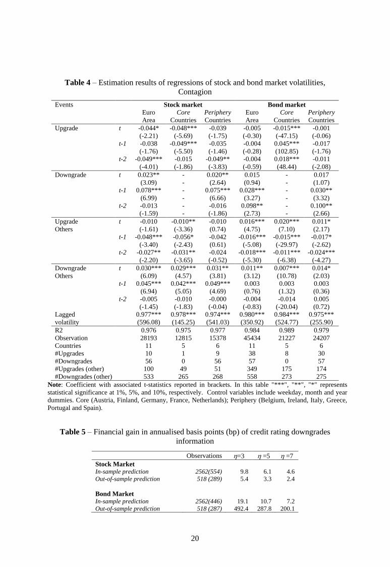
4.3. Contagion
In this subsection, we have restricted the analysis to Euro Area countries only and we
have included in the regressions the upgrades and downgrades rating announcements from
other countries in the Euro Area. We then divide the sample into the Core (Austria,
Finland, Germany, France, and Netherlands) and Periphery (Belgium, Ireland, Italy,
Greece, Portugal and Spain) countries.4 The volatility of both stock and bond markets of a
given country responds to announcements of agencies for other European countries. Table
4 shows that when a country has an upgrade, this is followed by a reduction of volatility in
the rest of the Euro-area, which is more pronounced in the Core countries. As for
downgrading movements, they increase the volatility of all other countries, specifically in
the periphery countries, although in the covered period there were no downgrades in the
core set of countries.
[Table 4]
5. Economic value of sovereign ratings’ information
5.1. The investor’s problem
In this section, we examine the economic implications of the impact of sovereign credit
ratings on the financial volatilities for the optimal diversification of risk. We assume that
the investors are risk averse with preferences defined over the conditional expectation and
the variance-covariance matrix of the asset returns.
To find the optimal conditional weight of the investment in each European asset (bonds
and equities), we consider the mean-variance behaviour characterized by an optimization
problem in which the efficient frontier can be described as the set of portfolios that satisfy
4 This distinction is in line notably with the results reported by Afonso, Arghyrou and Kontanikas (2012),
who split the euro area countries in a rather similar way, on the basis of a principal component analysis.

11
the constrained maximization problem below. The investor with an initial wealth of Wt=1
diversifies his or her portfolio between the European assets according to the following
problem:
2( ) ( )2
s.t. 1
t
p t p t
Tt
Max
e
(7)
where '1, ,( ,..., )t t n t , with n is the number of the European assets in the portfolio, is the
vector of portfolio weights, e is the 1n vector of ones, and
,
1
( )
n
p t i t i
i
w
(8)
2 2 2, , , , ,
1 1
( ) 2
n nT
p t t t i t i t i t ij t j tt
i i j n
(9)
are the mean and variance of portfolio return, respectively, with i and ij are the mean
asset return of the country i and the covariance between asset returns of countries i and j,
respectively. The solution to the maximization problem in (7) is given by the optimal
vector of weights:
1
1t
tT
t
eR
e e
,
1 1
1
1
T
t t
t T
t
ee
R
e e
, (10)
where the “multiplier” can be interpreted as a “risk aversion” coefficient and t is the
variance-covariance matrix of the vector of returns that corresponds to the n European
assets.
5.2. Financial gains from sovereign ratings’ information
We want to assess the financial gain of an investor who takes into account sovereign
credit ratings information for volatility modelling. We base our analysis on the following
expected utility function of the investor:
2( ( )) ( ) ( )2
t p t p tE U
. (11)
As in the previous subsection, the initial wealth is normalised to unity Wt=1, which
we can interpret as investing one euro at the beginning of the period. We define the gain gt
as the additional fraction of wealth necessary for an investor, who is not aware of the
sovereign credit rating information, to match the same level of utility of an investor who is

12
aware of this sovereign credit rating information. To get a simple analytical solution to our
problem, we assume that the additional fraction of wealth gt is not invested. Therefore, we
want the solution of the following equation5
*( ( ) ) ( ( ))bt t tE U g E U , (12)
where tb is the optimal vector of weights invested in the European assets when the
investor is not aware of the sovereign credit rating information, while t* is the optimal
vector of weights when the investor considers that information. Since gt is not random, the
mean-variance utility function implies that
*( (( )) ( (( ))bt t tg E U E U (13)
with
* 1*
*
* 1
( )t tt
T
t
eR w
w
e e
,
* 1 * 1
1*
* 1
T
t t
t T
t
ee
R
e e
(14)
where t* is the variance-covariance matrix in which the diagonal elements or the variance
terms are forecasted by taking into account the sovereign credit ratings information. In our
empirical application, we report the results for different values of risk aversion: =3, 5,
and 7. We choose these alternative values based on the empirical findings in the literature
(see, for example, French and Poterba, 1991).
To estimate the mean expected utility and the financial gain functions we proceed as
follows. First, we measure the volatilities of asset returns included in our dataset using the
approach described in section three. Second, we estimate the panel regressions:
, , , , 1 t-1 ,
0 0
log( ) log( ) X
k ki T
i t i j i t j j i t j i t i t
j j
down down
(15)
and
_ _ _
,, , 1 t-1log( ) log( ) XTi ti t i ti . (16)
The specifications in (15) and (16) correspond to models of volatilities with and
without taking into account the effect of sovereign credit ratings downgrade information on
stock and bond return volatilities, respectively. We abstract from the rating upgrades.
5If instead we assume that this fraction gt is invested, we will end up with a second order problem where the
solution will depend on the values of the coefficients, and in some circumstances, the solution does not exist.
13
Following section 4.3, we also include the dummies of downgrades from other countries,
,i
i t jdown . Here Xt-1 is still a vector of other control variables including dummy variables for
weekday and monthly effects. We include 10 lags of each.
Thereafter, we first recuperate the corresponding fitted-values of volatilities that we use
to estimate the weights t and t*, and then we compute the average values of the expected
utility functions ( (( ))btE U and
*( (( ))tE U , and of the financial gain gt. In order to focus on
the effect of sovereign credit ratings information on the volatilities, we use the
unconditional estimate of the mean returns and the correlation coefficients between the
asset returns. In every period and following Bollerslev (1990), we update the covariance
matrix to have a constant correlation equal to the unconditional correlation. Therefore, we
capture the impact of sovereign credit ratings’ information on the optimal portfolio
weights, and measure the financial gain gt due to the incorporation of such information.
5.3 Financial gains: empirical results
Our empirical results show the existence of a financial gain when we take into account
Sovereign credit ratings downgrade information for volatility modelling. Table 5 reports
the average financial gain in annualized basis points in the two weeks following
downgrade news. The in-sample prediction of the gains is based on the sample period
2002-2011 and includes 2562 days of which around 500 days are within 2 weeks of
downgrade announcements. The in-sample prediction analysis shows that the gains range
between 5 and 10 annualized basis points (bp) for stock market and between 7 and 19 for
bond markets.
[Table 5]
Another important issue to mention is that the financial gain is a decreasing function of
the degree of risk aversion. We find that a less risk averse agent outperforms a more risk
averse agent when both use the effect of credit ratings information on volatility to optimize
their portfolios. The fact that higher risk aversion portfolios might tend to be more biased
towards lower volatility countries can also explain this result. Indeed, such countries are in
practice less prone to downgrades, as we have seen in our dataset.
We also did an out-of-sample exercise to evaluate the financial gains. To predict the
financial gains we first predict the volatilities of all European assets that make up our
portfolio with and without using the credit rating information. Again, as in our in-sample

14
analysis, we only predict the volatilities, and thus we evaluate the mean returns and
correlation coefficients between European equity and bond returns at their unconditional
estimates. We consider one period (day) ahead static prediction during one year. For each
additional day within the last year of our sample, we re-estimate our volatility models
using the data available until that day, we make one-day ahead prediction of these
volatilities with and without using the Sovereign credit ratings information, and compute
the financial gains. The out-of-sample prediction is based on the last 2 years of the sample.
It includes 518 days of which 287 days are within 2 weeks of downgrade announcements.
Table 5 reports the results of the out-of-sample prediction of the financial gains. These
results show that the out-of-sample financial gains range between 2 and 6 bp for the stock
market and between 200 and 492 bps for the bond market. The reason for the performance
of the bond market is that it responds more significantly to downgrade news after two days,
while the stock market responds contemporaneously and with one lag. However, because
we assume that we can only restructure the portfolio one day after downgrades, thus we are
not using all the relevant information.
5.4 Risk management: value-at-risk
We also examine whether sovereign credit ratings’ information can help protect
investors against market risk. We compare the value-at-risk (VaR) of mean-variance
portfolios with and without taking into account the effect of credit ratings information on
stock and bond return volatilities. We discuss the empirical results below.
[Table 6]
Table 6 shows that for both in sample and out-of sample predictions, the value-at-risk
of portfolios that consider the information of sovereign credit ratings are smaller than the
ones of portfolios that do not take into account such information. It is true that the
difference is small in magnitude, but this could be very significant when we invest
important amounts of money. The result is similar in both stock and bond markets. In
addition, we find that the value-at-risk is decreasing with the degree of risk aversion.
6. Conclusion
We have used a panel fixed-effects analysis of daily EU stock market and sovereign
bond market returns to study the impacts of the three main rating agencies announcements
(S&P, Moody’s, Fitch) on financial markets volatility. Indeed, after the 2008-2009

15
financial and economic crises the volatility in capital markets increased in most EU
countries, both in sovereign debt and equity markets, challenging the euro area common
currency framework. The analysis covered the period between 2 January 1995, for some
countries, and 24 October 2011.
In practical terms, we have first filtered the negative and positive effects of market
returns on volatility via EGARCH models. Then, we have analysed the information content
of sovereign upgrades and downgrades on the volatility. Moreover, we then assessed the
potential financial gain for investors when considering such rating information on
theoretical portfolio diversification decisions.
Our main results can be summarised as follows. We have uncovered the existence of an
asymmetry of the effects of sovereign rating developments on volatility. Indeed, upgrades
do not have any significant effect on volatility, but sovereign downgrades increase stock
market volatility both contemporaneously and with one lag, and rise bonds volatility after
two lags. Interestingly, a rating upgrade in a given country reduces the volatility in the rest
of the Euro-area, particularly in the core countries. On the other hand, a downgrade
increases the volatility of all other countries, specifically in the periphery countries.
We have also shown the existence of a financial gain and risk reduction for portfolio
returns when taking into account sovereign credit ratings information for volatility
modelling. In addition, the financial gains are decreasing with the degree of risk aversion.
In addition, the value-at-risk of portfolios that consider the information of sovereign
credit ratings are smaller than the ones of portfolios that do not take such information into
account, with the value-at-risk decreasing with risk aversion.
16
References
Afonso, A., Arghyrou, M., Kontonikas, A. (2012). “The determinants of sovereign bond
yield spreads in the EMU”, mimeo.
Afonso, A., Furceri, D., Gomes, P. (2012). “Sovereign credit ratings and financial markets
linkages: application to European data”, Journal of International Money and Finance,
31 (3), 606-638.
Amira, K, Taamouti, A., Tsafack, G. (2011). “What drives international equity
correlations? Volatility or market direction?”, Journal of International Money and
Finance, Volume 30, Issue 6, pages 1234-1263.
Arezki, R., Candelon, B., Sy, A. (2011). “Sovereign rating news and financial markets
spillovers: Evidence from the European debt crisis", IMF Working Papers 11/68.
Bollerslev, T. (1990). “Modelling the coherence in short-run nominal exchange rates: a
multivariate generalized ARCH approach”, Review of Economics and Statistics, 72 (3),
492-505.
Borio, C., McCauley, R. (1996). “The economics of recent bond yield volatility”. BIS
Working Paper 45.
Christiansen, C., (2007). “Volatility-spillover effects in European bond markets”,
European Financial Management, 13 (5), 923-948.
Dufour, J-M, Garcia, R., Taamouti, A. (2912). “Measuring high-frequency causality
between returns, realized volatility and implied volatility”, Journal of Financial
Econometrics, Volume 10, Issue 1, pages 124-163.
Erb, C., Harvey, C., Viskanta, T. (1996). “Expected returns and volatility in 135
countries”. Journal of Portfolio Management, 22 (3), 46–58.
Ferreira, M., Gama, P. (2007), “Does sovereign debt ratings news spill over to
international stock markets”, Journal of Banking and Finance, 31, 3162-3182.
French, M., Poterba, J.M. (1991). “Investor diversification and international equity
markers”, American Economic Review, 81, 222-226.
Gande, A., Parsley, D. (2005). “News spillovers in the sovereign debt market”, Journal of
Financial Economics, 75 (3), 691-734.
Goeij, P., Marquering, W. (2004). “Modeling the conditional covariance between stock
and bond returns: A multivariate GARCH approach”, Journal of Financial
Econometrics, 2 (4), 531-564.
17
Heinke, V. (2006). “Credit spread volatility, bond ratings and the risk reduction effect of
watchlistings”, International Journal of Finance and Economics, 11, 293-303.
Hooper, V., Timothy, H., Kim, S. (2008). “Sovereign rating changes – Do they provide
new information to stock markets”, Economic Systems, 32 (2), 142-166.
Hull, J.C., Predescu, M., White, A. (2004). The relationship between credit default swap
spreads, bond yields, and credit rating announcements. Journal of Banking and
Finance 28, 2789-2811.
Ismailescu, J., Kazemi, H. (2010). “The reaction of emerging market credit default swap
spreads to sovereign credit rating changes”, Journal of Banking & Finance, 34 (12),
2861-2873.
Jones, C., Lamont, O., Lumsdaine, R. (1998). “Macroeconomic news and bond market
volatility”, Journal of Financial Economics, 47 (1998) 315-337.
Kräussl, R. (2005). “Do credit rating agencies add to the dynamics of emerging market
crises?” Journal of Financial Stability, 1 (3), 355-85.
Kilponen, J., Laakkonen, H., Vilminen, J. (2011). “Sovereign risk, uncertainty and policy”,
mimeo.
Micu, M., Remolona, E., Wooldridge, P. (2006). “The price impact of rating
announcements: which announcements matter?”. BIS Working paper.
Nelson, D.B. (1991). “Conditional heteroskedasticity in asset returns: A new approach”.
Econometrica, 59, 347-370.
Norden, L., Weber, M., (2004). “Informational efficiency of credit default swap and stock
markets: the impact of credit rating announcements”. Journal of Banking and Finance
28, 2813-2843.
Reisen, H., Maltzan, J. (1998). “Sovereign credit ratings, emerging market risk and
financial market volatility”. Intereconomics, 1(2), 73-82.
Reisen, H., Maltzan, J. (1999). “Boom and bust and sovereign ratings”. International
Finance, 2 (2), 273-29.

18
Table 1 – Summary of EGARCH estimation results (Equation (5))
Note: P-values are in brackets. In this table "***", "**", "*" represents statistical significance at 1%, 5%, and
10%, respectively.
Table 2 – Average of stock and sovereign yield market volatilities for different rating
categories
Rating Stock market volatility Yield volatility
S&P Moody’s Fitch S&P Moody’s Fitch
AAA 0.00023 0.00023 0.00023 0.00015 0.00014 0.00014
AA+ 0.00021 0.00020 0.00025 0.00011 0.00011 0.00011
AA 0.00019 0.00018 0.00013 0.00010 0.00013 0.00011
AA- 0.00014 0.00016 0.00027 0.00011 0.00007 0.00012
A+ 0.00024 0.00020 0.00029 0.00014 0.00037 0.00011
A 0.00022 0.00021 0.00017 0.00057 0.00016 0.00011
A- 0.00018 0.00027 0.00018 0.00019 0.00049 0.00018
BBB+ 0.00025 0.00020 0.00023 0.00023 0.00023 0.00022
BBB 0.00022 0.00021 0.00027 0.00029 0.00012 0.00035
Country Slope i Asymmetry i Persistence βi D.F. Obs. Gaps
Stock Market
Austria -0.074*** (0.000) 0.186*** (0.000) 0.981*** (0.000) 8.79 2564 0
Belgium -0.118*** (0.000) 0.159*** (0.000) 0.979*** (0.000) 11.08 2564 0
Finland -0.065*** (0.000) 0.105*** (0.000) 0.991*** (0.000) 6.41 2564 0
France -0.153*** (0.000) 0.102*** (0.000) 0.982*** (0.000) 15.44 2564 0
Germany -0.129*** (0.000) 0.113*** (0.000) 0.985*** (0.000) 11.41 2564 0
Greece -0.053*** (0.000) 0.158*** (0.000) 0.985*** (0.000) 7.78 2564 0
Ireland -0.072*** (0.000) 0.169*** (0.000) 0.986*** (0.000) 6.52 2564 0
Italy -0.109*** (0.000) 0.105*** (0.000) 0.989*** (0.000) 8.95 2564 0
Netherlands -0.131*** (0.000) 0.110*** (0.000) 0.987*** (0.000) 16.12 2564 0
Portugal -0.073*** (0.000) 0.219*** (0.000) 0.978*** (0.000) 6.46 2564 0
Spain -0.121*** (0.000) 0.127*** (0.000) 0.985*** (0.000) 8.05 2564 0
Bulgaria -0.028 (0.204) 0.589*** (0.000) 0.933*** (0.000) 3.31 2564 0
Czech Republic -0.061*** (0.000) 0.238*** (0.000) 0.969*** (0.000) 6.58 2564 0
Denmark -0.069*** (0.000) 0.155*** (0.000) 0.981*** (0.000) 7.91 2564 0
Yield
Austria 0.024*** (0.004) 0.134*** (0.000) 0.996*** (0.000) 7.27 4271 18
Belgium 0.021*** (0.010) 0.112*** (0.000) 0.995*** (0.000) 6.38 4034 1
Finland 0.026*** (0.009) 0.136*** (0.000) 0.994*** (0.000) 6.14 4372 8
France 0.032*** (0.000) 0.100*** (0.000) 0.997*** (0.000) 9.85 4020 2
Germany 0.031*** (0.000) 0.100*** (0.000) 0.998*** (0.000) 6.99 4380 4
Greece -0.029** (0.042) 0.192*** (0.000) 0.977*** (0.000) 9.85 3384 3
Ireland -0.006 (0.484) 0.117*** (0.000) 0.993*** (0.000) 5.69 4038 6
Italy -0.012 (0.213) 0.120*** (0.000) 0.987*** (0.000) 7.31 4014 0
Netherlands 0.029*** (0.000) 0.095*** (0.000) 0.998*** (0.000) 7.78 4031 2
Portugal -0.002 (0.818) 0.205*** (0.000) 0.988*** (0.000) 4.86 4312 25
Spain -0.004 (0.728) 0.100*** (0.000) 0.990*** (0.000) 5.32 3992 3
Czech Republic 0.029* (0.092) 0.383*** (0.001) 0.994*** (0.000) 3.32 2989 10
Denmark 0.019** (0.035) 0.156*** (0.000) 0.994*** (0.000) 5.00 4305 33
Hungary -0.082*** (0.004) 0.427*** (0.000) 0.943*** (0.000) 2.52 3160 25
Poland -0.030 (0.101) 0.347*** (0.000) 0.962*** (0.000) 3.38 3172 11
Sweden 0.033*** (0.000) 0.113*** (0.000) 0.997*** (0.000) 8.81 3223 37
United Kingdom 0.027*** (0.000) 0.077*** (0.000) 0.998*** (0.000) 8.89 3928 4

19
BBB- 0.00029 0.00032 0.00027 0.00041 0.00035 0.00058
<BB+ 0.00032 0.00025 0.00030 0.00065 0.00044 0.00046
Note: The volatility measures are based on EGARCH estimations in Table 1.
Table 3 – Estimation results of regressions of stock and bond market volatilities
(Equation (6)), Full sample
Note: Coefficients with associated t-statistics reported in brackets. In this table "***", "**", "*" represents
statistical significance at 1%, 5%, and 10%, respectively. Control variables include weekday, month and year
dummies. $ F-test for joint significance of the 3rd, 5th and 22nd lag.
Events Stock market Bond market (1) (2)
Upgrade t 0.019 0.029
(0.81) (0.18)
t-1 0.033 -0.012
(0.66) (-0.63)
t-2 -0.013 0.024
(-0.54) (0.83)
Downgrade t 0.026** 0.025
(2.30) (0.13)
t-1 0.072*** 0.021*
(4.02) (1.97)
t-2 0.008 0.112***
(0.59) (3.55)
Lagged 0.963*** 0.977***
volatility (156.87) (300.61)
R2 0.955 0.973
Observation 53821 66539
Countries 21 17
#Upgrades 74 65
#Downgrades 93 67
# Positive outlooks
# Negative outlooks
Test 3rd lag$ 0.42 (0.661) 0.30 (0.747)
Test 5th lag$ 8.06 (0.003) 0.64 (0.539)
Test 22nd lag$ 1.16 (0.334) 0.93 (0.414)
20
Table 4 – Estimation results of regressions of stock and bond market volatilities,
Contagion
Note: Coefficient with associated t-statistics reported in brackets. In this table "***", "**", "*" represents
statistical significance at 1%, 5%, and 10%, respectively. Control variables include weekday, month and year
dummies. Core (Austria, Finland, Germany, France, Netherlands); Periphery (Belgium, Ireland, Italy, Greece,
Portugal and Spain).
Table 5 – Financial gain in annualised basis points (bp) of credit rating downgrades
information
Events Stock market Bond market
Euro
Area
Core
Countries
Periphery
Countries
Euro
Area
Core
Countries
Periphery
Countries
Upgrade t -0.044* -0.048*** -0.039 -0.005 -0.015*** -0.001
(-2.21) (-5.69) (-1.75) (-0.30) (-47.15) (-0.06)
t-1 -0.038 -0.049*** -0.035 -0.004 0.045*** -0.017
(-1.76) (-5.50) (-1.46) (-0.28) (102.85) (-1.76)
t-2 -0.049*** -0.015 -0.049** -0.004 0.018*** -0.011
(-4.01) (-1.86) (-3.83) (-0.59) (48.44) (-2.08)
Downgrade t 0.023** - 0.020** 0.015 - 0.017
(3.09) - (2.64) (0.94) - (1.07)
t-1 0.078*** - 0.075*** 0.028*** - 0.030**
(6.99) - (6.66) (3.27) - (3.32)
t-2 -0.013 - -0.016 0.098** - 0.100**
(-1.59) - (-1.86) (2.73) - (2.66)
Upgrade t -0.010 -0.010** -0.010 0.016*** 0.020*** 0.011*
Others (-1.61) (-3.36) (0.74) (4.75) (7.10) (2.17)
t-1 -0.048*** -0.056* -0.042 -0.016*** -0.015*** -0.017*
(-3.40) (-2.43) (0.61) (-5.08) (-29.97) (-2.62)
t-2 -0.027** -0.031** -0.024 -0.018*** -0.011*** -0.024***
(-2.20) (-3.65) (-0.52) (-5.30) (-6.38) (-4.27)
Downgrade t 0.030*** 0.029*** 0.031** 0.011** 0.007*** 0.014*
Others (6.09) (4.57) (3.81) (3.12) (10.78) (2.03)
t-1 0.045*** 0.042*** 0.049*** 0.003 0.003 0.003
(6.94) (5.05) (4.69) (0.76) (1.32) (0.36)
t-2 -0.005 -0.010 -0.000 -0.004 -0.014 0.005
(-1.45) (-1.83) (-0.04) (-0.83) (-20.04) (0.72)
Lagged 0.977*** 0.978*** 0.974*** 0.980*** 0.984*** 0.975***
volatility (596.08) (145.25) (541.03) (350.92) (524.77) (255.90)
R2 0.976 0.975 0.977 0.984 0.989 0.979
Observation 28193 12815 15378 45434 21227 24207
Countries 11 5 6 11 5 6
#Upgrades 10 1 9 38 8 30
#Downgrades 56 0 56 57 0 57
#Upgrades (other) 100 49 51 349 175 174
#Downgrades (other) 533 265 268 558 273 275
Observations =3 =5 =7
Stock Market
In-sample prediction 2562(554) 9.8 6.1 4.6
Out-of-sample prediction 518 (289) 5.4 3.3 2.4
Bond Market
In-sample prediction 2562(446) 19.1 10.7 7.2
Out-of-sample prediction 518 (287) 492.4 287.8 200.1

21
Note: In this table "" represents the risk aversion parameter. These financial gains are within two weeks
of a downgrade. In brackets is the number of periods corresponding to two weeks after a downgrade.
Table 6 – Value at Risk with and without credit rating downgrades information
Note: In this table "" represents the risk aversion parameter. The value-at-risks are within two
weeks of a downgrade. These value-at-risks correspond to each unit invested in the mean-variance portfolios.
=3 =5 =7
Stock Market
In-sample prediction
Without rating information -0.0824 -0.0508 -0.0376
With rating information -0.0820 -0.0506 -0.0375
Out-of-sample prediction
Without rating information -0.1450 -0.0873 -0.0627
With rating information -0.1439 -0.0866 -0.0622
Bond Market
In-sample prediction
Without rating information -0.0509 -0.0342 -0.0279
With rating information -0.0505 -0.0340 -0.0278
Out-of-sample prediction
Without rating information -0.1605 -0.0961 -0.0689
With rating information -0.1583 -0.0949 -0.0680