1
Solving Flight Planning Problem for Airborne LiDAR Data
Acquisition Using Single and Multi-Objective Genetic
Algorithms
Ajay Dashora
1, Bharat Lohani
1 and Kalyanmoy Deb
2
1Department of Civil Engineering,
2Department of Mechanical Engineering
Indian Institute of Technology Kanpur
PIN 208016, Uttar Pradesh, India
{ajayd,blohani,deb}@iitk.ac.in
Kanpur Genetic Algorithms Laboratory Report Number 2013012 http://www.iitk.ac.in/kangal/pub.htm
Abstract: Genetic algorithms (GA) are being widely used as an evolutionary
optimization technique for solving optimization problems involving non-differentiable
objectives and constraints, large dimensional, multi-modal, overly constrained feasible
space and plagued with uncertainties and noise. However, to solve different kinds of
optimization problems, no single GA works the best and there is a need for customizing a
GA by using problem heuristics to solve a specific problem. For the airborne flight
planning problem, there is not much prior optimization studies made using any
optimization procedure including a GA. In this paper, we make an attempt to devise a
customized GA for solving the particular problem to arrive at a reasonably good solution.
A step-by-step procedure of the proposed GA is presented and every step of the
procedure is explained. Both single and multi-objective versions of the problem are
solved for a particular scenario of the flight planning for airborne LiDAR data acquisition
problem to demonstrate the use of a GA for such a real-world problem. The deductive
approach successfully identifies the appropriate configurations of GA. The paper
demonstrates how a systematic procedure of developing a customized optimization
procedure for solving a real-world problem involving mixed variables can be devised
using an evolutionary optimization procedure.
1. Introduction
Over the past two decades, there had been remarkable developments in the field of
evolutionary algorithms for solving real-world and complex optimization problems.

2
Genetic algorithms (GA) have been widely used for this purpose in a variety of
applications. The reasons for the success of GAs in such complex problem solving tasks
compared to their classical counterparts are that (i) their operators are flexible and
modifiable with problem information, (ii) capable of handling mixed variables, (iii)
capable of handling multi-modal problems, (iv) capable of utilizing information about
uncertainties in decision variables and noise in objective and constraint value
computations and (v) capable of working within restricted feasible search space.
In general, there are apparently two branches in the field of GA development and
research. The first branch deals with the development of new algorithms of GA by
modifying and configuring various genetic operators (i.e. selection, mutation, crossover,
elite preservation etc). The developed algorithms of GA are tested against the 30 standard
optimization problems. On the other hand, in the second branch of GA research, the
existing algorithms are applied on the optimization problems. In some of the studies,
researchers also prefer to implement the developed algorithms on the practical problems
and confirm their applicability and performance. However, as GA is explored and
configured specifically with an orientation to solve a particular class of problems, there is
no generic set of GA algorithms, which will certainly work for all problems. As a result,
there is no generic methodology available or suggested in the literature for the effective
use of GA for optimization. Further, there is no literature available that compiles a
complete line of framework suggesting a step-by-step procedure to solve a real-world
problem wherein the nature and behaviour of the objective and constraint functions is
unknown. In this paper, authors show a step-wise approach of exploration of GA that can
be adopted in general to solve many different classes of problems.
The process of GA consists of three sequential steps: initialization, objective and
constraints evaluation, and regeneration of new solutions. In the initialization step,
population (or samples) of design vectors are generated either randomly or using some
knowledge of previously known good solutions. The values of the objective and
constraint functions for these population members are evaluated in the second step. Based
on these function values, new population members are created using selection, crossover,
3
mutation and elite preservation techniques in the regeneration step. For a detail
explanation and description of the genetic operators, readers can refer a book on GA by
Goldberg [1] or more recent literature.
In this paper, we showcase how a generic framework of a GA can be modified to solve a
complex optimization problem in systematic manner. Flight planning, which is briefly
mentioned in Section 2, is one example of such complex problems. For solving any
optimization problem, procedures of handling mixed variables, initialization, and elite
preservation strategies are addressed in Section 3. In addition, parameter space niching,
which helps in maintaining much-desired diversity within a GA population is also
explored. The developed algorithms resulting from the combination of the various
strategies of variable handling, initialization, elite preservation techniques, and parameter
space niching are mentioned in Section 4 and investigated in Section 5 for a set of real-
world problems. Further, the importance of the use of multi-objective optimization is also
explained in Section 6 to develop a better understanding of the associated optimization
problem. Based on the observations of the optimization process for the real-world
problems, conclusions are derived in Section 7.
2. Flight Planning Problem
Flight planning problem for airborne LiDAR data acquisition, which is developed and
discussed in detail by Dashora [2], is considered as an example of a minimization problem.
The fitness function is formulated as time duration required to travel by an aircraft (or
helicopter) over a given area of interest (AOI) with given characteristics of terrain for
collecting the LiDAR data by means of an airborne laser scanner with navigation sensors
(Global Positioning System or GPS, and Inertial Measurement Unit or IMU). Along with the
LiDAR data, photographic or image data can also be collected with airborne digital camera
in the same flight. The starting point of flying operation over AOI is shown by point S in
Figure 1. Aircraft covers the AOI in the form of parallel strips, each of which has an effective
width equal to B . After covering a flight strip, which is at flying direction θ w.r.t. x-axis of
map, the aircraft navigates back to next strip by turning. The next strip may be reached by
consecutive turning mechanism, non-consecutive turning mechanism, or hybrid turning

4
mechanism. Consecutive turning mechanism is shown in Figure 1 below. In non-consecutive
turning mechanism, aircraft turns to a non-consecutive flight strip whereas hybrid turning
mechanism is a combination of consecutive and non-consecutive turning mechanisms. Once
all strips are covered and data collection is completed, aircraft exits from point E.
Fig. 1: Schematic view of AOI, flight strips and turnings [2]
The terrain surface or landscape enclosed by AOI may be flat or undulated. Similarly,
airborne LiDAR data can be captured with or without photographic (or image) data.
Therefore, the flight planning problem shows different variants for different terrain types
for both LiDAR data and simultaneous photographic data acquisition as test problems
(mentioned in Table 1).
Table 1: Problem Matrix with Problems Numbered from P1 to P4
Type of Terrain
Data Acquisition Flat Terrain Undulated Terrain
LiDAR data acquisition (alone) P1 P2
Simultaneous photographic data acquisition P3 P4
The number of constraints and consequently the complexities in flight planning problem
increase from problem P1 to P4. Problems P1 and P4 consist of minimum and maximum
number of constraints, respectively. In the following discussion, flight duration as fitness
θ
X
Y
Strips
Turnings
AOI
θ x
y
xx
yy
X
Y
X
Y
Strips
Flight Path
AOI
S
E
θ
X
Y
X
Y
Strips
Turnings
AOI
θ xx
yy
xx
yy
X
Y
X
Y
Strips
Flight Path
AOI
S
E
5
function and associated constraints are mentioned. Minimum constraints are specified for
the problem P1, while additional constraints, which are additional with respect to
previous problem, are specified. For example, the additional constraints for problem P2
are in addition to the constraints of problem P1. Similarly, the additional constraints for
problem P3 are in addition to the constraints of problem P2.
2.1 Problem Definition
As explained earlier, flight duration consists of the strip time and turning time. Turning
time is calculated as the minimum of the time durations required for consecutive turning,
non-consecutive turning, or hybrid turning. Considering the complexity, length, and
definition of the flight planning problem, only formulation for the objective and
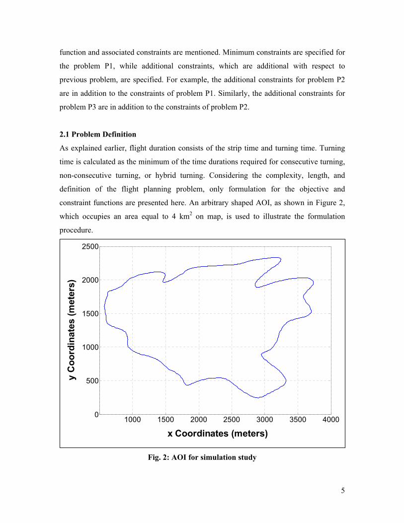
constraint functions are presented here. An arbitrary shaped AOI, as shown in Figure 2,
which occupies an area equal to 4 km2 on map, is used to illustrate the formulation
procedure.
Fig. 2: AOI for simulation study
1000 1500 2000 2500 3000 3500 40000
500
1000
1500
2000
2500
x Coordinates (meters)
y Coordinates (meters)

6
The objective function, i.e., flight duration (T ), can be expressed as:
T
n
i
Ri
Li
TV
XXi
L
T +=∑=1
),,(θ
… (1)
where
−=
y
x
Y
X
θθθθ
cossin
sincos … (2)
−=
B
YYN minmax … (3)
Nn= … (4)
=θ Flying direction w.r.t. x-axis on map in counter-clockwise direction,
=LiX Value of X coordinate of left edge (or left end) of thi flight strip (or flight line) in
rotated AOI,
=RiX Value of X coordinate of right edge (or right end) of thi flight strip (or flight line)
in rotated AOI,
=−= Ri
Lii XXL Length of thi flight strip (or flight line) from its start to end,
=maxY Maximum value of Y coordinate (or ordinate) of rotated AOI,
=minY Minimum value of Y coordinate (or ordinate) of rotated AOI, and
=TT Total turning time computed using a procedure given in technical report on turning
mechanisms [3]
Following constraints are considered for our problem. Generic constraints, which are
common to all problems, (i.e. P1, P2, P3, and P4), are described first:
Lρρ ≥
… (5)
d
A
SA
d
ddε≤
−
… (6)

7
( ) 01000 ≥− φf … (7)
Hp e≤σ … (8)
Vv e≤σ … (9)
ESDhH +≥ max … (10)
minmax HhH +≥ … (11)
Additional constraints exclusive for problems P1 and P3:
Uρρ ≤ … (12)
Additional constraints for problem P2 and P4:
Maxττ ρ ≤ … (13)
Constraints for problems P3 and P4:
−≤
V
nPGSDt
pxcx
ei
)1( … (14)
optc φφ ≥ … (15)
MaxGSDGSD≤ … (16)
where
,
=
VB
F
s
ρ … (17)
22
pp YXp σσσ += … (18)
pZv σσ = … (19)
HdtPR = … (20)
( )RR PP −= 1ρτ … (21)
sBPB )1( −= … (22)
φtan2 HBs = … (23)
)1()1(1 minPPP R −−−= … (24)
=
f
Vd A
2 … (25)

8
F
Bfd s
S
2= … (26)
=
c
p
f
sHGSD … (27)
≤ −
2tantan 1
max
opt
OCKφ
φ … (28)
−
−=
e
ecy
OCP
PK
1
1 … (29)
Recxecxcx PPPP )1( −+= … (30)
Parameters of optimization problems are half scan angle (φ ), scanning frequency ( f ),
flying height ( H ), speed (V ), flying direction (θ ), and PRF ( F ). The ranges of these
variables are presented in Table 2.
Table 2: Working Ranges of Parameters of Optimization Problems
Parameter Values
Range Least Count
H 80-3500 m Continuous
Θ 0-360º Continuous
V 45-72 m/s Continuous
f 1-70 Hz 1 Hz
ϕ 1-25º 1º
F
{33, 50, 70, 100} kHz (if 80 ≤ H ≤ 1100 m)
{33, 50, 70} kHz (if 1100 < H ≤ 1700 m)
{33, 50} kHz (if 1700 < H ≤ 2500 m)
{33} kHz (if 2500 < H ≤ 3500 m)
Discrete values
depending upon H
Note that the half scan angle (φ ) and scanning frequency ( f ) are integer variables.
Further, PRF ( F ) is also a discrete variable, but depending on the values of the flying
height ( H ), it takes different values. The remaining variables in the problem are
environmental constants presented in Table 3.
Table 3: Values of Constants in Optimization Problem
Parameter Value
ρL 10 points/m2
ρU 11 points/m2
τρ 30%
εd 10%

9
Pe 10%
eV 0.10 m
eH 0.15 m
GSDMax 0.15 m
Pecx 60%
Pecy 25%
βmax 25º
sp 0.000009 m
npx 4092
fc 0.06 m
tei 2.5 s
Mathematical expressions involved in the calculation of the total turning time are not
shown here. The technical report [3] explains the procedure for calculating the total
turning time. Similarly, calculations of ppp ZYX σσσ ,, are adopted from technical report
[4]. Interested readers may obtain the details from these reports.
According to the problem formulation and also by the ranges and nature of the objective
function and constraints, these are mathematically non-linear functions. In addition, the
objective function is a discontinuous function. Moreover, the variables of optimization
are integer, discrete and continuous variables, which are non-separable in the expressions
of objective function and constraints. Furthermore, more specifically, as the number of
options of values of PRF ( F ) depends upon the range of the flying height ( H ), it makes
the problem a variable-size optimization problem. Therefore, for solving this
optimization problem, use of genetic (or evolutionary) algorithm is inevitable.
3. Genetic Algorithm Essentials
Genetic algorithms (GAs) are flexible and versatile evolutionary optimization procedures
that can be applied to problems having non-differentiability, discontinuity and mixed
nature of variables. However, a GA is best applied if it is customized to solve a particular
problem. In the following subsections, we describe the essential features that can be
customized for an application and mention how they can be achieved for the flight
planning problem described above.

10
3.1 Fitness Function for Handling Objective Function and Constraints
The fitness function in the selection operator is simply calculated by equation (1).
Moreover, constraints are calculated using equations (5) to (16). Constraints are handled
by the parameter less approach presented in [5].
3.2 Variable Handling
Variables in the design vector that are either integer, discrete, or their combination can be
handled with GA. An integer variable, known with its upper and lower bound, is
generated randomly by a bit string of predefined length. The value of the variable is
obtained by decoding the bit string to decimal number. For example, the scanning
frequency (with a range of 1-70 Hz) can be generated by decoding the 7 bit binary
number which essentially results in integer numbers in the range of 0-127. The decoded
decimal values beyond the relevant range of variables are rejected by additional
inequality constraints. However, the GeneAS approach [6] advises to first generate all
variables as real continuous numbers and then obtain the value of the integer variables by
rounding the real number to the nearest integer. Moreover, PRF, which is a discrete
variable, is also referred by lookup table. For this arrangement, as shown by equations
(31) and (32), the continuous random number in range [0, 1] is mapped to discrete
numbers of lookup table as each discrete number in lookup table refers to a value of
discrete variable.
≤<
≤<
≤<
≤≤
=
35002500)(25.0
25001700)(5.0
17001100)(75.0
110080
Hu
Hu
Hu
Hu
u
F
F
F
F
F … (31)
≤<
≤<
≤<
≤≤
=
00.175.0100
75.050.070
50.025.050
25.000.033
F
F
F
F
ukHz
ukHz
ukHz
ukHz
F … (32)
11
In the forthcoming discussions, these two options of variable handling are abbreviated as
MCV (mixed or binary plus real-coded variables) and RCV (real-coded variables).
3.3 Sampling of Initial Population
A population of design vector is generated by ordinary random sampling (ORS) method.
However, instead of ORS, Latin hypercube sampling (LHS), which is a space filling
sampling technique, should also be employed and tested for real world problems [7].
LHS generates the multivariate samples by random paring of variables that exhibit the
space filling property and multivariate uniformity [8]. The original LHS method, of
McKay et al. [9], mentioned by Hess et al. [10] is adopted.
GA generates the values of a real parameter (say V ) between its given lower and upper
bounds using a random number. The thk sample or candidate of a population for a
parameter V , which is calculated using a random number ( kr ) in range [0, 1], can be
written as:
maxmin)1( VrVrV kkk +−= … (33)
For ordinary random sampling (ORS), the random number is a uniformly distributed
random number. Therefore,
kk ur = … (34)
However, for LHS, a random number kr is calculated by generating the non-repeating
random sequence of numbers 1 to m numbers as [11]-[12]:
−=
m
ur kk
k
π … (35)
Where
minV = Lower bound of variable V
maxV = Upper bound of variable V
kr = Random number for generating a random value of variable V
m = Population size (number of samples)
ku = Uniformly distributed random number in range [0, 1]
kπ = kth
member of non-repeating sequence

12
Random number ( kπ ) in non-repeating sequence and uniformly distributed random
number ( ku ) should be generated independently. The random permutations for each
variable ensure the random pairing of variables in multi-dimension [13].
The random non-repeating sequence of samples of a particular variable can be generated
by random permutation algorithm [14]. The random permutation algorithm shuffles a
sequence of m numbers randomly in an unbiased manner. Independently shuffled
sequences of m numbers for each variable individually generate random pairs of variables
with multivariate uniformity and space filling property [13].
3.4 Elite Preservation
For a particular generation, a design vector (or a candidate in a given population) which
provides THE optimal value (minimum value for a minimization problem) is named as
‘current best’. However, the mechanism of elitism prefers to preserve the candidate that
brings the optimal fitness function over the generations. The preserved candidate is called
the ‘best ever’. After a particular generation, if the ‘best ever’ is found to be inferior to
the ‘current best’, the value stored in the ‘best ever’ is updated by the value of the
‘current best’. According to the elitism, the ‘best ever’ unconditionally participates in
next generation by replacing another candidate in a population. Induction of elitism
avoids the straying of the evaluation process towards a sub-optimal solution and thus
enhances the probability of detection of global optimal solution. However, on the other
hand, the elitism principle reduces the diversity of population over generations and
thereby it is also suspected of early or premature convergence.
Replacement of a candidate in population by the ‘best ever’ is performed with different
strategies. In this paper, including the elite-less evaluation, the following four
methodologies are used for elitism.
(a) No elites (NE): Elitism is not adopted and the ‘best ever’ is neither evaluated nor
recorded. In other words, only the ‘current best’ is evaluated in a generation for reporting
13
purpose. ‘Current best’ can not affect the next generation directly as its unconditional
participation in the next generation is not allowed.
(b) ‘Best ever’ replaces the current worst (BRCW): Contrary to the ‘current best’, the
‘current worst’ is defined as a candidate that provides the worst value of fitness function
(maximum value for a minimization problem) in a generation. The ‘current worst’ is
replaced by the ‘best ever’ [15].
(c) 'Best ever' replaces a candidate by niching (BRCN): The ‘best ever’ replaces a
candidate which is most similar to the ‘best ever’ itself. This process is also known as the
objective space niching (OSN). For evaluating the most similar candidate, first a specific
percentage (say 20%) of population is chosen randomly from the population. Among the
chosen candidates, the most similar candidate has minimum Euclidean distance in
parameter space from the ‘best ever’. The percentages of chosen candidates may vary
from 0 to 100%. However, 0% arrangement resembles to ‘No elites (NE)’ and increasing
percentage of chosen candidates will raise the computation cost considerably.
(d) ‘Best ever’ replaces a candidate randomly (BRCR): The ‘best ever’ replaces a
candidate which is chosen randomly from a population [15].
3.5 Parameter Space Niching
The discussion so far considers the possibility of multiple local optima while assuming
prominent and dominating global optima compared to local ones. However, during the
evaluation process by GA, it is possible that in a certain generation, the majority of
population members are attracted towards a local optimum and very few are attracted
towards a global optimum. Consequently, due to the higher number of population
members being attracted towards the local optimum, the GA will be biased towards the
local optima in the subsequent generations. It generally happens for competing optima
which are spread across the parameter space that the majority of the population
candidates may be attracted towards a local optimum. As a result, the evaluation process
of GA may get trapped around a local optimum. Due to this bias, a global optimum that is

14
located by a smaller number of candidates is apparently ignored. Therefore, in a multi-
modal problem, even the ‘best ever’ evaluated over many generations may possibly be a
local optimum which may be an inferior result.
The problem of trapping of the GA solution in a local optimum for a multi-modal
optimization problem is resolved by parameter space niching [16]. The parameter-space
niching considers objective or fitness values of candidates, which are available in the
vicinity of a local optimum. According to the expected number of optima in a parameter
space, Deb [17] suggests to assume the parameter space divided amongst the optima and
considers a hyper-sphere around an optimum. Degrading the fitness values of all
candidates falling around a local optimum within the hyper-sphere by a predefined factor
gives an opportunity to other candidates to play a significant role in the subsequent
generations. The following formula is mentioned to calculate the value of niching radius
of hyper sphere ( shareσ ) in normalized parameter space [17] (on page 155):
( )
=
pshareq
/1
5.0σ … (36)
where
p = Number of parameters in optimization problem
q = Number of expected optima in complete parameter space
In order to implement parameter space niching, Deb [17] recommends to use q in the
range of 5-10 for the real-world problems. However, our purpose of using parameter
space niching is to preserve the diversity in the population so that few solutions, which
are found in the global basin of attraction do not get ignored, we assume that the problem
has q=10 optima and accordingly we choose shareσ equals to 0.340646 in this study.
The next section discusses the proposed configuration of a GA using the above strategies
and the subsequent section implements the derived algorithm for solving the flight
planning problem for airborne LiDAR data acquisition.

15
4. Proposed GA
The discussed options for configuration of GA create several combinations of algorithms
as mentioned strategies are independent and thus can be implemented individually. The
following table consolidates all discussed options (or strategies) suggested.
Table 4: Configuration Parameters of RGA Code
S.N. Strategy (number of options) Details (abbreviated names) of options
1. Variable handling (2) BCV, RCV
2. Sampling (2) ORS, LHS
3. Elitism (4) NE, BRWC, BRCN, BRCR
4. Parameter space niching or PSN (2) PSN or Without PSN
The options in the above table suggest 32 permutations which can be tested on any real-
world problem. In view of various algorithms, it is required to investigate the possible
configurations of GA and determine a configuration that can be universally accepted for
an optimization problem. In order to implement these algorithms, the Real-Coded
Genetic Algorithms (RGA) code and Non-dominated Sorting Genetic Algorithms-II
(NSGA-II) code [18], which are available online from KanGAL’s website
(http://www.iitk.ac.in/kangal/codes.shtml) for solving the single objective and multi-
objective optimization problems, respectively, are used in this study.
The RGA and NSGA-II codes that respectively optimize the single and multi-objective
optimization problems with normalized constraints, handle continuous and discrete
variables as real and binary coded design variables, respectively. All the details regarding
the initialization of population, selection process, crossover, mutation and constraint
handing strategies are commented in the available codes. The population is generated in
the initialization process by ordinary random sampling (ORS) method, as discussed in
Section 3.3. The selection is performed by the tournament selection method. The
available code uses the single point crossover [1] and simulated binary crossover (or
SBX) [19] for binary and real variables, respectively. The bit-wise mutation is carried out
for the binary coded GA while the polynomial mutation [20] is used for the real coded
GA. The constraints are handled using the Deb's parameter-less approach [5]. For a
multi-modal problem, the code also has a provision for parameter space niching [17]
which is already discussed in detail in the previous section. The codes also provide a file

16
output with solution of design vector and values of fitness function and constraints.
Specific details about the RGA code and NSGA-II code are explicitly mentioned in Deb
[21] and Deb et al. [18], respectively.
The resulting combinations of test problems (P1 to P4) and 32 different algorithms,
described in previous sections, result in a large number of options to be evaluated. Thus
we desire a deductive approach in which 10 algorithms (A1-A10) are considered with 4
problems (P1 to P4). The purpose of testing multiple algorithms, whose genesis is
discussed in the above section, is to identify a set of algorithms that show the best
performance on the test problems. According to the performance, appropriate algorithms
can be identified and prioritized. As a result, the available default RGA code, as
algorithm A1, is utilized at first and based on its performance new algorithms are derived.
The forthcoming discussion details the results of single objective constrained
minimization of test problems. Moreover, next section also describes a diligent approach
of implementing the GA algorithms to solve a minimization problem.
5. Results of Single Objective Optimization
The following discussion designs a set of algorithms with the default RGA code as the
first or base algorithm. The simulations are performed on computer machines having
‘Intel Core 2 Q9550 Quad processors (2.83 GHz)’ and ‘Intel Core i3 530 processors (2.93
GHz)’. The statistical measures (minimum, maximum, average and standard deviation) of
flight duration are evaluated for 30 runs of each algorithm. Moreover, number of outliers
is also detected manually. Lower value of standard deviation and less number of outliers
show the convergence and consistency, respectively, in the results obtained by the
algorithm.
The default RGA code facilitates the use of binary coded integer and real coded
continuous variables with ORS and no elite preservation. As the half scan angle (φ ) and
scan frequency ( f ) are integer variables, the mixed variable approach (combination of
integer and continuous variables) is used. In order to decide the better variable handling
strategy, the default algorithm with mixed variables (binary coded discrete variables and

17
real coded continuous variables) and a population count equal to 60 are first employed
with four elite preservation strategies against the first test problem P1. None of the four
algorithms perform as desired and thus results are not presented here. Further increasing
the population count to 200, which is more than 3 times the recommended value, also do
not find an acceptable solution. The probable reason is that GA is restricted to explore the
discrete variables amongst the integer numbers with standard indices of crossover and
mutation operators, as exploring and regenerating in the limited integer numbers cannot
reach to a specific value. However, as has been discussed earlier, all variables including
integer ones, can also be treated as real coded variables [6]. When integer variables are
coded as rounded real variables, the first three algorithms (A1, A2, A3) can find feasible
results for problem P1 with a population count of 60. A result generated by RGA code is
declared outlier if the optimum value of the flight duration is not similar to the majority
of the flight duration values for other runs. Increasing the population to 120 and 200
reduced both the number of outliers and the standard deviation of the flight duration.
However, algorithm A4 cannot find any feasible result with any population count (60,
120, and 200). On the other hand, the solutions determined by the algorithm A2 are
feasible, though all solutions appeared as outliers when compared with the results of A1
and A3. The results are tabulated below with the details of the algorithms. Table 5 below
also indicates the number of outliers and feasible results.
Table 5: Statistical Results of Simulation of Test Problem P1 with Algorithms A1 to A3
Problem P1: LiDAR Data Acquisition Alone on Flat Terrain
Algorithm Minimum
(seconds)
Maximum
(seconds) Average
(seconds)
Standard
Dev.
(seconds)
Outliers/
Feasible
Results
Population = 60
A1
(RCV+ORS+NE ) 1572.888 1598.427 1580.223 7.828 11/30
A2
(RCV+ORS+BCRW) 1820.020 1841.703 1822.215 5.303 0/30
A3
(RCV+ORS+BRCR) 1572.513 1603.716 1576.998 7.4 11/30
Population = 120
A1
(RCV+ORS+NE ) 1572.557 1652.099 1585.951 21.784 5/30
A2
(RCV+ORS+BCRW) 1573.154 1635.079 1585.295 18.442 6/30
A3
(RCV+ORS+BRCR) 1572.552 1583.484 1575.007 30.037 4/30
Population = 200

18
A1
(RCV+ORS+NE ) 1572.77 1655.552 1585.177 19.83 5/30
A2
(RCV+ORS+BCRW) 1573.152 1655.552 1584.701 18.341 4/30
A3
(RCV+ORS+BRCR) 1572.749 1587.435 1573.854 2.739 2/30
The analysis of performance of the algorithms A1 to A4 for test problem P1 indicates that
three strategies demonstrate the capability of optimization. For algorithm A2, for the
population count of 60, none of the results are outliers but the obtained fitness value is
worse than that of other algorithms. This may be due to the premature convergence,
which generally happens if the population can not explore the complete parameter space
and consequently reaches to inferior optimum. However, for population count of 120 and
200, the effect of the premature convergence reduces. On the other hand, the fourth
strategy (algorithm A4) can not find any feasible solution in all 30 runs. The probable
reason is difficult to quote without attempting this algorithm for other problems.
With the performance shown above, the simulations are performed for the test problem
P2 with all four algorithms. All four algorithms are able to resolve the problem of
minimization for problem P2. However, the number of outliers for the population counts
of 60 and 120 for over 30 runs are in the range of 9-15. Therefore, the results for the
population count of 200 only are shown in Table 6.
Table 6: Statistical Results of Simulation of Test Problem P2 with Algorithms A1 to A4
Problem P2: LiDAR Data Acquisition Alone on Undulated Terrain
Population = 200
Algorithm Minimum
(seconds)
Maximum
(seconds) Average
(seconds)
Standard
Dev.
(seconds)
Outliers/
Feasible
Results
A1
(RCV+ORS+NE ) 1874.318 1994.195 1918.523 40.679 6/30
A2
(RCV+ORS+BCRW) 1874.318 1994.195 1918.523 40.678 6/30
A3
(RCV+ORS+BRCR) 1864.442 1902.133 1873..662 7.656 3/30
A4
(RCV+ORS+BRCN) 1863.670 1903.895 1872.565 8.153 3/30
As shown in Table 6, algorithms A3 and A4 performed considerably well when
compared to algorithm A1 and A2 against the criteria of standard deviation and number

19
of outliers. Algorithms A1 and A2 show low consistency figures (higher number of
outliers) and higher standard deviation values. The low consistency may be due to the
multiple optima being located very close to each other and GA is occasionally detecting
any one of them. Moreover, as stated earlier, if inferior optima appear in large numbers,
these may be detected as optima with a higher probability. Considering this possibility of
multiple local optimums, parameter space niching is deployed and the algorithms A1 and
A2 are upgraded. However, no significant improvement is observed even with this
modification. On the other hand, in anticipation of further improvement in the
performance, algorithms A3 and A4 are upgraded to the algorithms A5 and A6 by
adopting the parameter space niching. The niching radius, expressed by equation (36), is
calculated for an anticipated number of multi-optimums (i.e., equal to 10). Once again, no
significant improvement is observed in the minimum value of the objective function and
in the consistency of results. Moreover, algorithm A6, which is an up-gradation of the
algorithm A4, show slight degradation in the results compared to results of A4. On the
other hand, parameter space niching is successful in reducing the magnitudes of outliers.
Table 7: Statistical Results of Simulation of Test Problem P2 with Algorithms A5 to A6
Problem P2: LiDAR Data Acquisition Alone on Undulated Terrain
Population= 200, Niching Radius = 0.340646;
Algorithm Minimum
(seconds)
Maximum
(seconds) Average
(seconds)
Standard
Dev.
(seconds)
Outliers/
Feasible
Results
A5
(RCV+ORS+BRCR+PSN) 1865.403 1902.398 1874.327 9.593 3/30
A6
(RCV+ORS+BRCN+PSN) 1865.180 1952.882 1879.162 19.275 5/30
A critical observation of the minimum values of the fitness function (Tables 6 and 7),
obtained by the algorithms A3, A4, A5 and A6, indicates that each algorithm obtains
similar values of the minimum flight duration at least once over 30 runs. Therefore, a
more detail analysis of the chosen algorithms is required to investigate what features of
the algorithms are important.
The standard deviation values are shown in Tables 6 and 7, which suggest that GA is
severely affected by bias. The anticipated bias, which may be developed in GA
implementation at any stage, from its initialization to the end of last generation, is

20
generally overcome by increasing the mutation probability or population count.
Increasing the mutation probability in algorithm A5 and A6 degrades the results.
However, increasing the population count to 200 or higher reduces the standard deviation
of fitness values. A higher number of samples generated with increased population count
perhaps explored the parameter space more rigorously and therefore, it further indicates
that bias is inducted by the sampling method. Consequently, the sampling by LHS is
adopted for initialization of the population. The upgraded algorithms are A7, A8, A9 and
A10. Algorithms A7 and A8 utilize the LHS alone whereas additionally the parameter
space niching is also applied in algorithms A9 and A10. As sampling method of GA is
changed, the simulations for all four algorithms (A7, A8, A9 and A10) are attempted for
population count of 60, 120 and 200. However, for a population count of 60 and 120, the
numbers of outliers are in the range of 5-8 for A7 and 5-17 for A8, respectively.
Additionally, with the same population count of 60 and 120 for algorithms A9 and A10,
the number of outliers is slightly less. However, for population count of 200, all four
algorithms perform almost in similar manner as there are no major differences in the
values of outliers or standard deviations. Results of population count 200 are presented in
Tables 8 and 9.
Table 8: Statistical Results of Simulation of Test Problem P2 with Algorithms A7 to A8
Problem P2: LiDAR Data Acquisition Alone on Undulated Terrain
Population = 200
Algorithm Minimum
(seconds)
Maximum
(seconds) Average
(seconds)
Standard
Dev.
(seconds)
Outliers/
Feasible
Results
A7
(RCV+LHS+BRCR) 1865.051 1880.460 1873.351 5.427 4/30
A8
(RCV+LHS+BRCN) 1865.251 1902.768 1872.735 8.619 5/30
Table 9: Statistical Results of Simulation of Test Problem P2 with Algorithms A9 to A10
Problem P2: LiDAR Data Acquisition Alone on Undulated Terrain
Population = 200; Niching Radius = 0.340646
Algorithm Minimum
(seconds)
Maximum
(seconds) Average
(seconds)
Standard
Dev.
(seconds)
Outliers/
Feasible
Results
A9
(RCV+LHS+BRCR+PSN) 1865.066 1882.392 1874.327 5.047 4/30
A10
(RCV+LHS+BRCN+PSN) 1864.308 1886.427 1871.788 6.188 4/30

21
As is evident from the results presented in Table 9, an insignificant improvement is
observed due to the parameter space niching. Consequently, due to the extra
computational load in comparison to the gain in the result by the parameter space
niching, the algorithms A9 and A10 are discarded. As a result, the algorithms A7 and A8
are applied on the test problems P3 and P4. The results are shown in Tables 10 and 11.
Table 10: Statistical Results of Simulation of Test Problem P3 with Algorithms A7 to A8
Problem P3: LiDAR and Photographic Data Acquisition on Flat Terrain
Population = 200
Algorithm Minimum
(seconds)
Maximum
(seconds) Average
(seconds)
Standard
Dev.
(seconds)
Outliers/
Feasible
Results
A7
(RCV+LHS+BRCR) 1572.604 1576.200 1573.309 0.748 1/30
A8
(RCV+LHS+BRCN) 1572.560 1577.897 1573.531 1.109 0/30
Table 11: Statistical Results of Simulation of Test Problem P4 with Algorithms A7 to A8
Problem P4: LiDAR and Photographic Data Acquisition on Undulated Terrain
Population=200
Algorithm Minimum
(seconds)
Maximum
(seconds) Average
(seconds)
Standard
Dev.
(seconds)
Outliers/
Feasible
Results
A7
(RCV+LHS+BRCR) 1941.770 1948.097 1944.136 1.804 1/30
A8
(RCV+LHS+BRCN) 1942.317 1949.325 1944.609 2.069 0/30
5.1 Selection of the Best Algorithm
Apart from the observations on performance and analysis of algorithms for various
problems (P1 to P4), selection of algorithm is equally important. An algorithm that show
minimum number of outliers (consistency) and determines the flight duration with
minimum variation (convergence) is better than other algorithms.
As shown previously that for problems P2, P3, and P4, standard deviations of the flight
duration values over 30 runs by algorithms A7 and A8 are considerably less compared to
the other algorithms. Moreover, a pattern of reduction in the numbers of outliers, when
population increases, is also observed. As a result, it can be inferred that algorithms A7
and A8 are able to solve the minimization problem with maximum number of constraints
(i.e. problem P4). However, considering the additional calculations in algorithm A8, due

22
to the objective space niching, the algorithm A7 appears a good trade off in performance
and speed. There is a possibility of achieving better performance of algorithm A8 by
increasing the fraction of population considered for evaluating the most similar candidate
for the ‘best ever’. However, due to the smaller standard deviation observed in the fitness
values and flight planning parameter values, and less computational load in decision
making process, the algorithm A7 can be accepted as a better algorithm without
hesitation.
6. Results of Multi-Objective Optimization
As indicated earlier, when a user wants to understand the variation of flight duration or
trade-off against the constraints, the single-objective minimization approach sometimes
cannot suffice the purpose. An alternative approach considers the potential of multi-
objective optimization, which allows integration of two or more conflicting objectives in
a single framework. The multi-objective optimization is performed by the NSGA-II code
here. The error in LiDAR data has an inverse relationship with the flight duration, as
improving the former decreases the latter [2]. As both planimetric and altimetric errors
increase with the decrease in flight duration, the 3D error minimization is considered as
the second objective in the NSGA-II code. Alike 3D errors, the effective swath ( B ) is
also conflicting with the flight duration. However, flight planners are generally not
interested to know about the trade-off between effective swath and flight duration.
Therefore, in this paper, authors show the compromise solutions of flight duration with
altimetric and planimetric errors in detail.
6.1 Bi-objective Optimization by NSGA-II Code
With LHS method and RCV for parameters, simulations are run by NSGA-II code for
300 generations and a population count of 2,000. The results showing trade-off between
the two conflicting objectives are obtained by NSGA-II code with the flight duration
being the first objective (on y-axis) and one of the altimetric error or planimetric error
being as the second objective (on x-axis).
23
The problems P1 to P4 involve all the mentioned variables (i.e., planimetric error,
altimetric error), though the multi-objective optimization by NSGA-II code is performed
only for problems P2 and P4 as both contain the maximum number of constraints for
simultaneous LiDAR and photographic data acquisition. When the problems, P2 or P4,
are solved as a single-objective constrained minimization problem, the original
planimetric and altimetric errors are treated as constraints representing the minimal
requirement of desired data. In multi-objective optimization, in addition to be used as
constraints, one of altimetric or planimetric error is also considered as second objective in
NSGA-II code. The fronts of optimal values showing the compromising results for two
variables against the flight duration are plotted as shown in Figures 3 to 6. We discuss
these plots in the following paragraph.
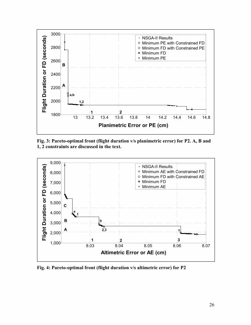
The NSGA-II code plots the values of flight duration for all values of the vertical and
horizontal errors (1σ) which are less than 10 cm and 15 cm, respectively, as the vertical
and horizontal errors are restricted up to these values. Moreover in all plots, the zones
with no points indicate gaps (mainly due to the absence of any feasible solution in these
regions, which we demonstrate in the next paragraph) in the obtained front. Figures 3 to 4
and Figures 5 to 6 are drawn for problems P2 and P4, respectively. For problem P4, in
comparison to problem P2, due to higher number of constraints, the feasible zones are
smaller for all variables (second objective) as is evident from the comparison of figures.
Before making any inference using these plots, it should be first confirmed whether the
front containing compromise solutions are truly Pareto-optimal. A Pareto-optimal front
contains trade-off solutions that cannot be improved for both objectives simultaneously.
Although mathematical optimality conditions involving derivatives of objectives and
constraints and certain regularity conditions are needed to prove Pareto-optimality of
every point, here we make an attempt to build confidence about their optimality by
solving several single-objective epsilon-constraint (EC) problems. EC method, which is
briefly explained by Mavrotas [22], minimizes the first objective as a single-objective
problem with an additional constraint on the second objective that is conflicting with the
first one. For example, the flight duration is minimized by the RGA code with a

24
constraint that planimetric error should be less than or equal to 13.6 cm (for example) in
Figure 3. If a Pareto-optimal solution exists between the gap (having planimetric error
within 13.1cm and 14.3cm), the above epsilon-constraint optimization problem should
find it. This would then validate the gap indicated by the NSGA-II solutions. In the
figure, points obtained by NSGA-II showing the trade-off between the FD and
planimetric errors are connected by firm lines to show the non-dominated region in the
upper half of the figure. Constraints on FD and errors are shown by horizontal and
vertical dashed lines, respectively.
EC method is deployed with 2,000 population members and is run for 300 generations
with algorithm A7. Solutions are obtained by minimizing the flight duration under the
original constraints of altimetric and planimetric errors and with the above additional
constraint (planimetric error is less than or equal to 13.6 cm (marked as constraint 2 in
Figure 3)). Interestingly, the obtained solution does not lie within the gap, instead it lies
close to the planimetric error of 13.1 (marked as ‘2’ in the figure 3) – a solution also
obtained by NSGA-II. This indicates that a feasible solution does not exist within the gap
and this is the reason NSGA-II found a fragmented set of trade-off solutions. One other
epsilon-constraint formulation is performed with an additional planimetric error limited
to 13.2 cm (constraint marked as 1 in Figure 3) and the obtained solution is close to one
of the NSGA-II solution (marked as ‘1’). Constraints on flight duration at two different
values (2,200 and 2,500 sec) are tried next and planimetric error objective is minimized.
Corresponding optimized solutions are marked as ‘a’ and ‘b’, respectively. All these
independent single-objective minimizations amply indicate that there does not lie any
feasible solution in the gaps present in the fragmented NSGA-II front.
To further validate the extreme solutions, we perform independent minimization of each
objective with the original constraints alone. The optimized solutions are marked with a
star (FD minimization) and with a ‘x’ (PE minimization). The optimized solutions are
slightly worse than the respective extreme NSGA-II solutions. The presence of gaps
certainly makes the search process difficult and this study demonstrates the efficacy of
the suggested NSGA-II approach for solving the flight planning optimization problem.

25
Similar studies of epsilon-constraint minimization to validate observed gaps in NSGA-II
fronts and individual objective minimization to validate the extreme NSGA-II solutions
are performed for other three bi-objective optimization problems in Figures 4, 5 and 6.
Table 12 displays extreme values of FD and altimetric error, and the salient points
obtained by EC method by constraining the FD and altimetric error for problem P4.
Table 12: Extreme Values and Results of EC Method for Problem P4
Constraint Flight Duration
(FD) (seconds)
Altimetric Error
(AE) (cm)
Constrained
Marked by
Solution
Marked by
Minimizing the Altimetric Error (AE) with Constrained Flight Duration (FD)
FD≤ 2100 seconds 2090.80 8.0612 Line A Point a
FD≤ 2800 seconds 2799.66 8.0373 Line B Point b
FD≤ 4500 seconds 2837.46 8.0373 Line C Point c
Minimizing the Flight Duration (FD) with Constrained Altimetric Error (AE)
AE≤ 8.03 cm 3899.01 8.0241 Line 1 Point 1
AE≤ 8.04 cm 2727.41 8.0385 Line 2 Point 2
AE≤ 8.06 cm 2727.32 8.0385 Line 3 Point 3
Extreme Values: Minimum Values of Flight Duration (FD) and Altimetric Error (AE)
Minimizing FD 1931.94 8.0729 Star (*)
Minimizing AE 5334.03 8.0239 Cross (x)
As indicated in Table 12, the values obtained by EC method are marked in Figure 6 by
alphabets a, b, c and numbers 1, 2, 3. Interestingly, as evident from the Table 12, point 2
and 3, and b and c are clustered.
26
Fig. 3: Pareto-optimal front (flight duration v/s planimetric error) for P2. A, B and
1, 2 constraints are discussed in the text.
Fig. 4: Pareto-optimal front (flight duration v/s altimetric error) for P2
13 13.2 13.4 13.6 13.8 14 14.2 14.4 14.6 14.81800
2000
2200
2400
2600
2800
3000
Planimetric Error or PE (cm)
Flight Duration or FD (seconds)
NSGA-II Results
Minimum PE with Constrained FD
Minimum FD with Constrained PE
Minimum FD
Minimum PE
A
B
a,b
1,2
1 2
8.03 8.04 8.05 8.06 8.071,000
2,000
3,000
4,000
5,000
6,000
7,000
8,000
9,000
Altimetric Error or AE (cm)
Flight Duration or FD (seconds)
NSGA-II Results
Minimum AE with Constrained FD
Minimum FD with Constrained AE
Minimum FD
Minimum AE
2 31
B
C
A
b
1
c
a
2,3

27
Fig. 5: Pareto-optimal front (flight duration v/s planimetric error) for P4
Fig. 6: Pareto-optimal front (flight duration v/s altimetric error) for P4
12.9 12.95 13 13.05 13.1 13.15 13.2 13.25 13.31800
2000
2200
2400
2600
2800
3000
Planimetric Error or PE (cm)
Flight Duration or FD (seconds)
NSGA-II Result
Minimum FD with Constrained PE
Minimum PE with Constrained FD
Minimum FD
Minimum PE
A
B
1
2 3
a,b
2 31
8.02 8.03 8.04 8.05 8.06 8.07 8.08
2000
3000
4000
5000
6000
Altimetric Error or AE (cm)
Flight Duration or FD (seconds)
NSGA-II Results
Minimized AE with Constrained FD
Minimized FD with Constrained AE
Minimum FD
Minimum AEC
A
2 3
B
1
2,3
1
b,c
a
28
Having obtained confidence in the NSGA-II front, the next section presents a general
analysis and interpretation of these results as well as the physical significance of these
results for the flight planning problem.
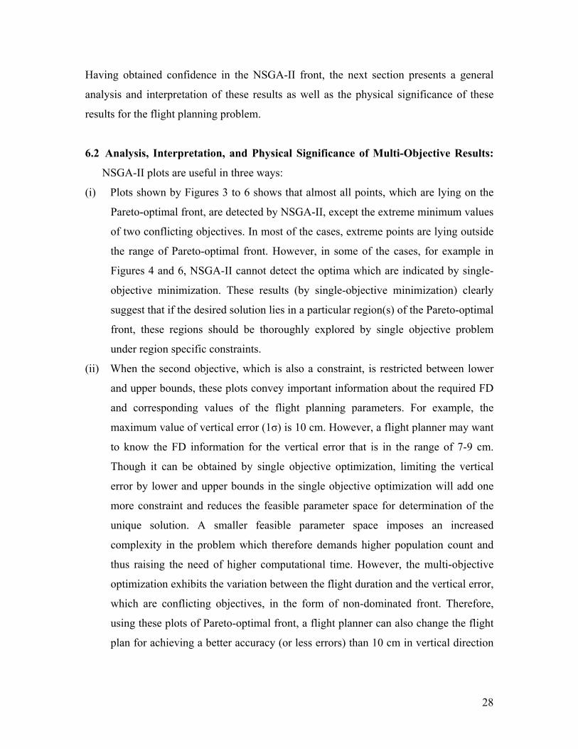
6.2 Analysis, Interpretation, and Physical Significance of Multi-Objective Results:
NSGA-II plots are useful in three ways:
(i) Plots shown by Figures 3 to 6 shows that almost all points, which are lying on the
Pareto-optimal front, are detected by NSGA-II, except the extreme minimum values
of two conflicting objectives. In most of the cases, extreme points are lying outside
the range of Pareto-optimal front. However, in some of the cases, for example in
Figures 4 and 6, NSGA-II cannot detect the optima which are indicated by single-
objective minimization. These results (by single-objective minimization) clearly
suggest that if the desired solution lies in a particular region(s) of the Pareto-optimal
front, these regions should be thoroughly explored by single objective problem
under region specific constraints.
(ii) When the second objective, which is also a constraint, is restricted between lower
and upper bounds, these plots convey important information about the required FD
and corresponding values of the flight planning parameters. For example, the
maximum value of vertical error (1σ) is 10 cm. However, a flight planner may want
to know the FD information for the vertical error that is in the range of 7-9 cm.
Though it can be obtained by single objective optimization, limiting the vertical
error by lower and upper bounds in the single objective optimization will add one
more constraint and reduces the feasible parameter space for determination of the
unique solution. A smaller feasible parameter space imposes an increased
complexity in the problem which therefore demands higher population count and
thus raising the need of higher computational time. However, the multi-objective
optimization exhibits the variation between the flight duration and the vertical error,
which are conflicting objectives, in the form of non-dominated front. Therefore,
using these plots of Pareto-optimal front, a flight planner can also change the flight
plan for achieving a better accuracy (or less errors) than 10 cm in vertical direction

29
with the information about the respective increase in the flight duration. Similarly,
this analysis can also be done for horizontal error, and other conflicting objectives.
(iii) On the curve of non-dominated front, where no data are available, indicates
infeasible parameter space i.e. all constraints are not satisfied. Using this
information, a flight planner can visualize the available infeasible zones in the
parameter space. For example, Figure 4 shows that an altimetric error in LiDAR
data in the range of 8.04-8.06 cm, under the current set up of the constraints of the
problem, cannot be achieved. Similarly, Figure 3 demonstrates that a planimetric
error in the range of 13.2-14.2 cm cannot be achieved for the specifications of
problem P2 because all active constraints are not satisfied for this range of
planimetric errors. This information is also useful for deciding the limits of a
conflicting variable in a specific range in single objective optimization. Similar
inferences can be made with Figures 5 to 6 for problem P4.
(iv) It should be noted that the multi-objective optimization demonstrates the variation
between two conflicting objectives and thus a decision should not be made about
the other objectives. With two particular objectives, the variations of remaining
objectives are not considered. For example, as the flight duration and altimetric
error are considered two objectives, the multi-objective optimization by NSGA-II
code will show the variation of these two variables only as shown in Figure 4 (and
6). Therefore, as discussed earlier, a decision that fixes the values of these
objectives using Figure 4 (and 6) can be made. However, by multi-objective
optimization, any one conflicting objective with respect to flight duration can be
considered for decision making. Therefore, multi-objective optimization is not a
substitute of the single objective optimization but both optimization techniques
complement each other.
7. Conclusions
This paper addresses various processes of the GA (e.g. variable handling, sampling, elite
preservations, and parameter space niching) and their configurations (or algorithms).
Further, the paper successfully outlined a step-by-step procedure to implement the
developed algorithms. In order to test the algorithm, it is implemented on a complicated

30
four variants of optimization problem of flight planning for airborne LiDAR data
acquisition. Four variants of the flight planning problem consist of different number of
constraints. Performance of the algorithms are analyzed by consistency and convergence
criteria using various statistical measures, like minimum, maximum, average and
standard deviation of fitness function over multiple runs. Using a deductive approach,
better algorithms are developed to solve a complicated single and multi-objective
optimization version of the flight planning problem. It is noticed that continuous
variables of optimization problem, initialized by Latin hypercube sampling, elite
preservation by BRCR, and without parameter-space niching successfully detects the
minimum in most runs. Moreover, as GA is least expected to show the biased behavior,
the parameter space niching should not be attempted at first. Before applying the
parameter space niching for single objective problems, it is recommended to exhaust all
other possibilities of configuration of parameters of GA. Multi-objective optimization by
NSGA-II code of flight planning problem provided the trade-off between the conflicting
objectives (i.e. flight duration against planimetric and altimetric errors in LiDAR data).
This case study remains as a testimony to developing efficient customized single and
multi-objective optimization algorithms for solving real-world problems.
Acknowledgements
Authors are thankful to Varun Jindal and Ashutosh for helping in development of
physical model of flight planning problem.
References
[1] Goldberg, D.E., 1989. A Gentle Introduction to Genetic Algorithms, in Genetic Algorithms in
Search, Optimization, and Machine Learning. Pearson Education Asia, Delhi (India), pp 1-25.
[2] Dashora, A., 2012. PhD Dissertation: Optimization System for Flight Planning for Airborne LiDAR
Data Acquisition, Indian Institute of Technology Kanpur, Kanpur (India), 216 pages.
[3] Dashora, A. and Lohani, B., 2013. Turning Time Calculation for Airborne Surveys, KanGAL Report
No 2013010, Indian Institute of Technology Kanpur, Kanpur (India).
URL: http://www.iitk.ac.in/kangal/reports.shtml (last accessed May 26, 2013)
[4] Dashora, A. and Lohani, B., 2013. Calculation of Error Propagated in Airborne LiDAR Data,
KanGAL Report No 2013011, Indian Institute of Technology Kanpur, Kanpur (India).
URL: http://www.iitk.ac.in/kangal/reports.shtml (last accessed May 26, 2013)

31
[5] Deb, K., 2000. An Efficient Constraint Handling Method for Genetic Algorithms, Computer
Methods in Applied Mechanics and Engineering, Vol. 186(2-4), pp 311–338.
[6] Deb, K. and Goyal, M., 1996. A Combined Genetic Adaptive Search (GeneAS) for Engineering
Design, Computer Science and Informatics, Vol. 26(4), pp 30–45.
[7] Devay, K.R., 2008. Latin Hypercube Sampling and Pattern Search in Magnetic Field Optimization
Problems, IEEE Transactions on Magnetics, Vol. 44(6), pp 974-977.
[8] Deutsch, J.L. and Deutsch, C.V., 2012. Latin Hypercube Sampling with Multidimensional
Uniformity, Journal of Statistical Planning and Inference, Vol. 142, pp 763-772.
[9] McKay, M. D., Beckman, R.J. and Conover, W.J., 1979. A Comparison of Three Methods for
Selecting Values of Input Variables in the Analysis of Output from a Computer, Technometrics, Vol
21(2), pp 239-245.
[10] Hess, S., Train, K.E. and Polak, J.W., 2006. On the Use of a Modified Latin Hypercube Sampling
(MLHS) Method in the Estimation of a Mixed Logit Model for Vehicle Choice, Transportation
Research Part B 40, pp 147–163.
[11] Tong, 2006. Tong, C., 2006. Refinement Strategies for Stratified Sampling Methods, Reliability
Engineering and System Safety, Vol. 91, pp 1257–1265.
[12] Petelet, M., Iooss, B., Asserin, O. and Loredo, A., 2010. Latin Hypercube Sampling with Inequality
Constraints, Advances in Statistical Analysis, Vol. 94, pp 325-339.
[13] Sallaberry, J., Helton, J.C. and Hora, S.C., 2006. Extension of Latin Hypercube Sampling with
Correlated Variables, Sandia Report No. ‘SAND2006-6135’, Sandia National Laboratories, United
States Department of Energy, Albuquerque, New Mexico (USA), 48 pages.
URL: http://dakota.sandia.gov/papers/IncremLHS.pdf (last accessed September 7, 2012)
[14] Durstenfeld, R., 1964. Algorithm 235: Random Permutation, Communications of ACM, Vol. 7(7),
page 420.
[15] Deb, K. 2005. A Population-Based Algorithm-Generator for Real-Parameter Optimization, in F.
Herrera and M. Lozano (eds.), Special Issue on "Real Coded Genetic Algorithms: Foundations,
Models and Operators", Soft Computing Journal, Vol. 9, pp 236-253.
[16] Goldberg, D.E. and Richardson, J., 1987. Genetic Algorithms for Sharing for Multimodal Function
Optimization, Proceedings of the 2nd International Conference on Genetic Algorithms, Lawrence
Erlbaum Associates, pp 41-49.
[17] Deb, K., 2001. Multi-Objective Optimization using Evolutionary Algorithms, John Wiley & Sons
Inc., Chichester (UK), 515 pages.
[18] Deb, K., Pratap, A., Agarwal, S., and Meyarivan, T., 2002. A Fast and Elitist Multi-objective
Genetic Algorithm: NSGA-II, IEEE Transactions on Evolutionary Computation, Vol. 6(2), pp 182-
197.
[19] Deb, K., and Kumar, A., 1995. Real-coded Genetic Algorithms with Simulated Binary Crossover:
Studies on Multi-modal and Multi-objective Problems, Complex Systems, Vol. 9, pp 431-454.
[20] Deb, K., and Deb, D., 2012. Analyzing Mutation Schemes for Real-Parameter Genetic Algorithms, KanGAL Report Number 2012016, Indian Institute of Technology Kanpur, Kanpur (India). URL: http://www.iitk.ac.in/kangal/reports.shtml (last accessed May 26, 2013)

32
[21] Deb, K., 1995. Ch-6: Nontraditional Optimization Algorithms (pp 290-359), in Optimization for
Engineering Design: Algorithms and Examples, PHI Learning Pvt. Limited, New Delhi (India), 10th
print, 396 pages.
[22] Mavrotas, G., 2009. Effective Implementation of the E-Constraint Method in Multi-Objective
Mathematical Programming Problems, Applied Mathematics and Computation, Vol. 213, pp 455-
465.