Signal-Specialized Parameterization for Piecewise Linear Reconstruction
Geetika Tewari, Harvard UniversityJohn Snyder, Microsoft Research Pedro V. Sander, ATI Research
Steven J. Gortler, Harvard University Hugues Hoppe, Microsoft Research

Two Scenarios
Authoring: map a texture image onto a surfaceAuthoring: map a texture image onto a surfaceAuthoring: map a texture image onto a surfaceAuthoring: map a texture image onto a surface
Sampling: store an existing surface signalSampling: store an existing surface signalSampling: store an existing surface signalSampling: store an existing surface signal

Signal Source
Procedural texture
High-resolution image texture
High-resolution geometry
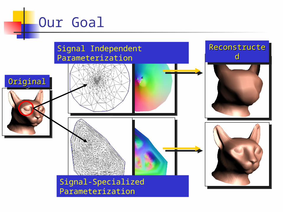
Our Goal
ReconstructedReconstructedReconstructedReconstructed
OriginalOriginalOriginalOriginal
Signal-Specialized Parameterization
Signal Independent Parameterization

Related Work
Pinkall and Polthier. 1993. Computing Discrete Minimal Surfaces… Eck et al. 1995. Multiresolution Analysis of Arbitrary Meshes. Hormann and Greiner. 2000. MIPS – global parameterization method. Levy et al. 2002. Least Squares Conformal Maps. Desbrun et al. 2002. Intrinsic Parameterizations of Surface Meshes.
Sloan et al. 1998. Importance Driven Texture Coordinate Optimization.
Hunter & Cohen. 2000. Uniform Frequency Images. Balmelli et al. 2002. Space Optimized Texture Maps. Sander et al. 2002. Signal-Specialized Parameterization.
Signal Specialized Parameterization
Signal Independent Parameterization
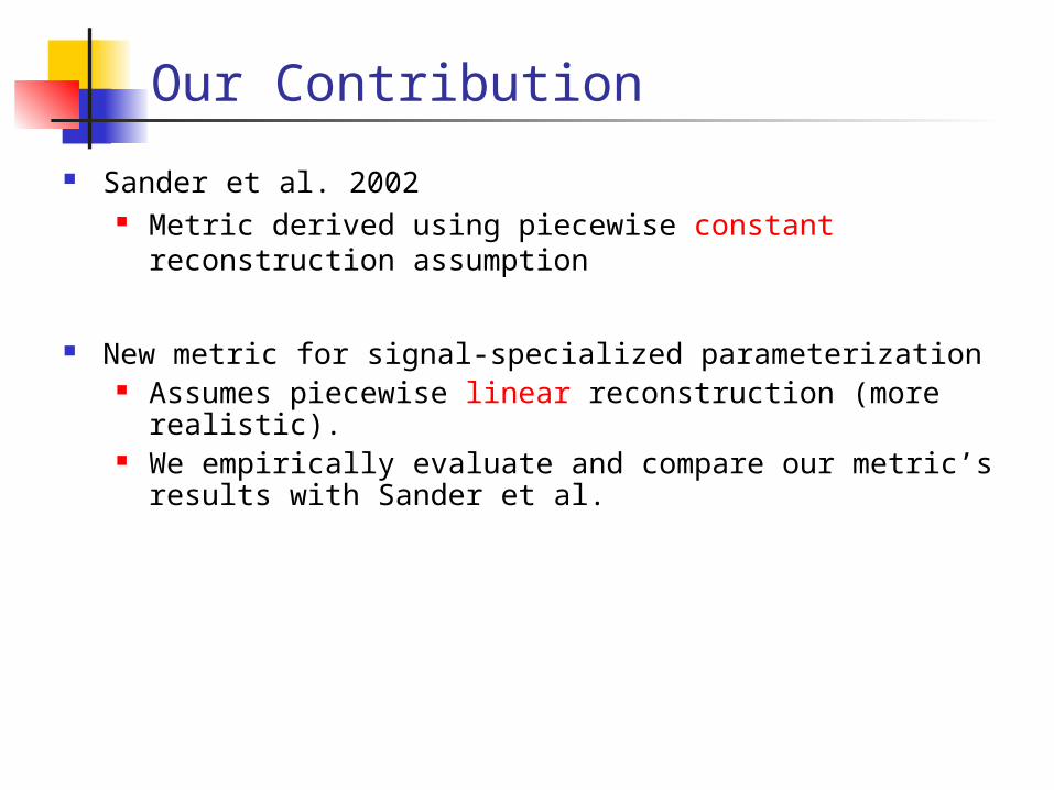
Our Contribution
Sander et al. 2002 Metric derived using piecewise constant reconstruction
assumption
New metric for signal-specialized parameterization Assumes piecewise linear reconstruction (more realistic). We empirically evaluate and compare our metric’s results
with Sander et al.

Signal-Specialized Parameterization
ff
h = g . fh = g . f gg
surfacesurface
Signal rangeSignal rangeSignal rangeSignal range
domaindomain originaloriginaloriginaloriginal
reconstructedreconstructedreconstructedreconstructed
signal signal approximation approximation
errorerror
signal signal approximation approximation
errorerror

Piecewise constant
reconstruction
Piecewise constant
reconstruction
Signal-Specialized Parameterization
originaloriginaloriginaloriginal
reconstructedreconstructedreconstructedreconstructed
signal signal approximation approximation
errorerror
signal signal approximation approximation
errorerror
Signal Signal rangerange
Signal Signal rangerange
ff
h = g . fh = g . f gg
domaindomaindomaindomain
Signal height range on domain scanline
surfacesurfacesurfacesurface
Piecewise linear
reconstruction
Piecewise linear
reconstruction

Derivation of Metric
Signal approximation error
= h – (reconstructed h)
Texture domainTexture domain
ij
si
tj
t
s
Single sample
Neighborhood (single red square of area 2)2(
How well is approximated when reconstructed from a discrete sampling over the texture domain D?
fg h

Metric: how to derive
Define error at each point Represent signal as Taylor series Assume reconstruction is linear Error is dominated by 2nd order term
Derive error integrated over ij
Sum ij over whole surface
In the limit, (more and more samples) this sum becomes an integral
... And error vanishes Divide by to obtain convergence
rate Use this as “energy” metric
Partition integral into sum over triangles.
ij
si
tj
t
s
4
Texture domainTexture domain

Error Metric
),(),(),(
),(
),(
),(
iittiistiiss
iitt
iist
iiss
tshtshtsh
tsh
tsh
tsh
Define 3 by 3 matrix at each point (squares of second derivatives).
),( ii tsH
),(
),(
),(
),(
),(
),(
),(
),(
),(
ii
ii
ii
ii
ii
ii
ii
ii
ii
ts
ts
ts
ts
ts
ts
ts
ts
ts
),(),(),(
),(
),(
),(
1iittiistiiss
n
k
iiktt
iikst
iikss
tshtshtsh
tsh
tsh
tsh

Error Metric
),(
),(
),(
),(
),(
),(
),(
),(
),(
),(),(),(
),(
),(
),(
),(
ii
ii
ii
ii
ii
ii
ii
ii
ii
iittiistiiss
iitt
iist
iiss
ii
ts
ts
ts
ts
ts
ts
ts
ts
ts
tshtshtsh
tsh
tsh
tsh
tsH
)(~
)(~)(~
)(~)(~)(
~
)(~)(
~)(~
),(ˆ),()(~
),(
i
i
i
i
i
i
i
i
i
ts
i
i
tsAdtsHH
Integrate over each triangle to get “tilded” 3 by 3 matrix, for each triangle

Error Metric
),(
),(
),(
),(
),(
),(
),(
),(
),(
),(),(),(
),(
),(
),(
),(
ii
ii
ii
ii
ii
ii
ii
ii
ii
iittiistiiss
iitt
iist
iiss
ii
ts
ts
ts
ts
ts
ts
ts
ts
ts
tshtshtsh
tsh
tsh
tsh
tsH
)(~
)(~)(~
)(~)(~)(
~
)(~)(
~)(~
),(ˆ),()(~
),(
i
i
i
i
i
i
i
i
i
ts
i
i
tsAdtsHH
)(~
)(~)(~
)(~)(~)(
~
)(~)(
~)(~
)(~
)(~
S
S
S
S
S
S
S
S
S
HSHTi
i
Sum over all all triangles to get “tilded” H for entire surface

Error Metric
),(
),(
),(
),(
),(
),(
),(
),(
),(
),(),(),(
),(
),(
),(
),(
ii
ii
ii
ii
ii
ii
ii
ii
ii
iittiistiiss
iitt
iist
iiss
ii
ts
ts
ts
ts
ts
ts
ts
ts
ts
tshtshtsh
tsh
tsh
tsh
tsH
)(~
)(~)(~
)(~)(~)(
~
)(~)(
~)(~
),(ˆ),()(~
),(
i
i
i
i
i
i
i
i
i
ts
i
i
tsAdtsHH
)(~
)(~)(~
)(~)(~)(
~
)(~)(
~)(~
)(~
)(~
S
S
S
S
S
S
S
S
S
HSHTi
i
)(5
1~)(~
9
4)(~
9
2)(~
5
1)( SSSSSE
Add up 4 of the terms in the matrix (the entire matrix is kept for the upcoming affine transform rule).

Numerical Computation of Metric
We need to compute
Compute Compute Numerical Integration of HNumerical Integration of H
Compute H:Compute H: Function FittingFunction Fitting Isometric flatteningIsometric flattening
its
i
i
i
i
i
i
i
i
i
i tsAdtsHH),(
)(~
)(~)(~
)(~)(~)(
~
)(~)(
~)(~
),(ˆ),()(~
)(~
iH
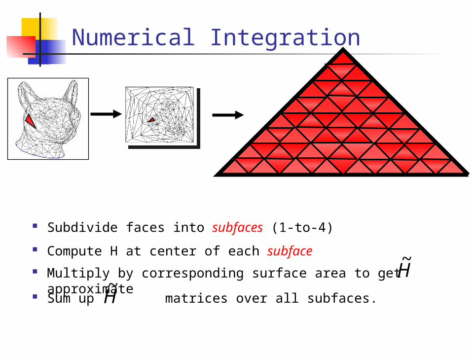
Subdivide faces into subfaces (1-to-4)
Numerical Integration
Compute H at center of each subface
Sum up matrices over all subfaces.H~
Multiply by corresponding surface area to get approximate H~

Function Fitting
Assumption: the signal can be point sampled at parameter domain points (s,t)
least squares solver
FEtDsCstBtAs 22
FEDCBA ,,,,,
BCA
B
C
A
H 22
2
2
Second derivatives:
CBA ,2,2
n
k
kkk
k
k
k
BCA
B
C
A
H1
)2()2(
)2(
)2(

Choosing Points for Local Signal Fitting
During local signal fitting in numerical computation of H: How do we choose (s,t) coordinates for local signal fitting?
Canonical parameterization
(0,0) (1,0)
(0,1)

Isometric Flattening
It might be necessary to include samples over neighboring faces
Isometrically map face to (s,t). Isometrically flatten three neighbors. For 3 subdivisions we use 15 points.

Parametrization algorithm
Start with uniform parametrization. Iterate: for each vertex, try random line searches Minimize:
But: This is too time consuming on large meshes - Need multigrid
method. We modify the parameterization algorithm by Sander et al
[2002]
)(5
1~)(~
9
4)(~
9
2)(~
5
1)( SSSSSE

Neighborhood Optimization
OptimizatioOptimizationn
OptimizatioOptimizationn
H4’H4
1H
2H
5H
3H
5H
2H
3H
1H
4H
4H

Affine Transformation Rule
needs to be evaluated every time we change the parameterization.
Useful trick: Precompute with respect to some chosen s,t coordinates.
When triangle is warped, can be updated in closed form without resampling the signal (affine transform rule).
New New parameterizationparameterization
Initial (fixed) Initial (fixed) parameterizationparameterization
Affine Affine transformtransform
H~
H~
H~
H~
H~

Affine Transformation Rule
J matrix: Jacobian of the mapping from new triangle parameterization to old.
Linear system of untransformed second derivatives:
Thus H can be transformed via:
Summary:
New parameterization
yielding
tt
st
ss
tt
st
ss
tt
st
ss
h
h
h
Q
h
h
h
J
JJ
J
JJ
JJJJ
JJ
J
JJ
J
h
h
h
222
2221
221
2212
21122211
2111
212
1211
211
2
)(
2
TTttstss
tt
st
ss
QQQhhh
h
h
h
Q
TQHQH
TQSHQH )(~~
Initial (fixed) Initial (fixed) parameterizationparameterization

Relationship to Approximation Theory
Goal (Approximation Theory): Approximate some bivariate scalar function g(x,y) using linear interpolation with a given number of triangles over the (x,y) plane.
Result Can minimize the error of piecewise linear approximation (L2 sense) by [Nadler, 1986]:
As number of triangles An optimal orientation of a triangle is given by the
eigenvectors of the Hessian of g An optimal aspect ratio of a triangle is given by:
2
1
min
max

Correspondence with Nadler’s Result
Hessian of g:
Nadler’s result: optimal triangles are axis aligned and with aspect ratio
Nadler’s solution minimizes our energy functional!
If this bivariate scalar function is quadratic: FByAxyxg 22),(
B
A
20
02
2
1
B
A

Experiments
Signal Approximation Error (SAE): RMS difference between the original signal and its bilinear reconstruction.
We compare our results with the signal-stretch metric of Sander et al. [2002]
reconstructionreconstruction
reconstructedreconstructedreconstructedreconstructed
signasignall
surfacsurfacee
Parameterization Parameterization algorithmalgorithm
Hardware: Bilinear
Assume: linear

1
10
100
1.E+02 1.E+03 1.E+04 1.E+05 1.E+06
Texture size (texels)
Sig
na
l ap
pro
x. e
rro
r
Signal Error - Piecewise Constant Reconstruction
Signal Error - Piecewise Linear Reconstruction
Parasaur's head: 3,870 vertex parameterization
Parasaur’s head
Sander et al.
Ours
Factor of 4 savings in texture area
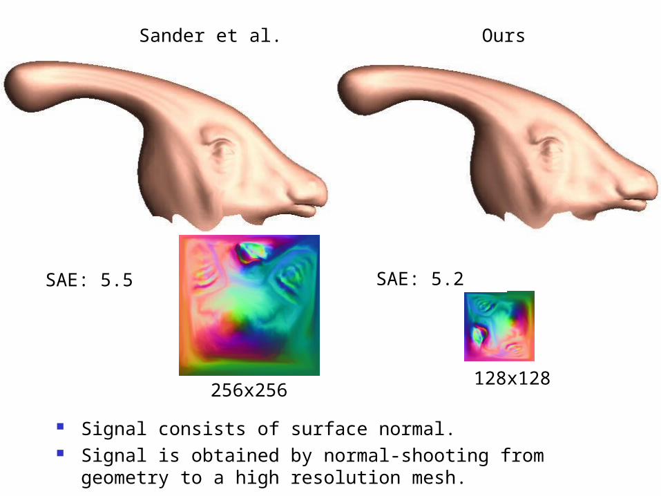
256x256128x128
SAE: 5.5 SAE: 5.2
Ours
Signal consists of surface normal. Signal is obtained by normal-shooting from geometry to a
high resolution mesh.
Sander et al.
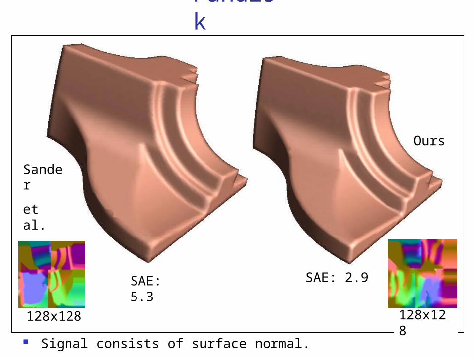
Fandisk
128x128
SAE: 5.3
Signal consists of surface normal.
128x128
SAE: 2.9
Ours
Sander
et al.

Fandisk
OursSander et al.

Comparison with Previous Work
ComparisonMeasure
Terzopoulos & Vasilescue
1991
Sloan et al. 1998
Hunter &
Cohen 2000
Balmelli et al.2002
Sander et al.2002
Ours
Applications
Adaptive sampling
and reconstructio
n
Compact Texture Maps
MetricAdjustable
spring energy
Wavelets &
User- specified
scalar importanc
e
Fourier Wavelets
SAE(1st
order Taylor)
SAE(2nd order
Taylor)
Remarks
Requires optimizati
on procedure
Allows user
control
Fast greedy algorith
m
Texture deviation error
Constant re-
construction
Captures signal
anisotropy Faster
Linear re-
constriction
Captures signal
anisotropy
Slower by 1-2
minutes

Conclusions and Future Work
Future Directions Perceptual measures More optimal treatment of signal discontinuity Non-asymptotic analysis Optimization of texture samples
Significant savings in texture space for the same level of signal approximation error compared to metric by Sander et al.

Thank you…