Wirtschaftswissenschaftliche Diskussionspapiere
Sectoral and Regional Expansion of Emissions Trading
Christoph Böhringer, Bouwe Dijkstra, and Knut Einar Rosendahl
V – 337 – 11
June 2011
Institut für Volkswirtschaftslehre Universität Oldenburg, D-26111 Oldenburg
1
Sectoral and Regional Expansion of Emissions Trading
Christoph Böhringera, Bouwe Dijkstrab and Knut Einar Rosendahlc
Abstract: We consider an international emissions trading scheme with partial sectoral and
regional coverage. Sectoral and regional expansion of the trading scheme is beneficial in
aggregate, but not necessarily for individual countries. We simulate international CO2
emission quota markets using marginal abatement cost functions and the Copenhagen 2020
climate policy targets for selected countries that strategically allocate emissions in a bid to
manipulate the quota price. Quota exporters and importers generally have conflicting interests
about admitting more countries to the trading coalition, and our results indicate that some
countries may lose substantially when the coalition expands in terms of new countries. For a
given coalition, expanding sectoral coverage makes most countries better off, but some
countries (notably the USA and Russia) may lose out due to loss of strategic advantages. In
general, exporters tend to have stronger strategic power than importers.
Keywords: Emissions Trading; Allocation of Quotas; Strategic Behavior
JEL: C61; C72; Q25
Acknowledgement: We are grateful to Odd Godal, Carsten Helm and Erling Holmøy for
valuable comments on an earlier draft. Financial support from the Renergi programme of the
Research Council of Norway and the German Research Foundation (BO 1713/5-1) is
appreciated.
a University of Oldenburg. E-mail: [email protected] b University of Nottingham. E-mail: [email protected] c Research Department, Statistics Norway. E-mail: [email protected]
2
1. Introduction
International emissions trading is considered a key instrument to combat global warming
because it promotes cost-effectiveness of emission abatement and thereby increases political
feasibility of stringent emission reduction objectives.
Since 2005 the EU has been a forerunner in the implementation and operation of a multi-
jurisdictional emissions trading scheme. While the EU emissions trading scheme (EU ETS)
has been critically observed as a “New Grand Experiment” (Kruger and Pizer, 2004) in the
early stage, it is meanwhile perceived as a success story which could be the nucleus for a
gradually expanding system towards global coverage (Convery, 2009). As a matter of fact, the
EU strongly pushes policy initiatives to link the EU ETS with other regional greenhouse gas
cap-and-trade systems outside the EU (EU, 2007).1
With respect to cost-effectiveness of emission abatement, an important characteristic of the
EU ETS is its incomplete coverage. The EU ETS focuses on energy-intensive installations
and thereby covers only around 40% of the EU-wide greenhouse gas emissions. To achieve its
reduction target of 20% by 2020 (compared to 1990 emission levels), the EU must undertake
complementary regulation of emission sources outside the EU ETS. The segmentation of
emission regulation into one EU-wide ETS market and multiple national non-ETS markets
has given rise to concerns on adverse implications for cost-effectiveness of EU emission
abatement: While the allocation of emission allowances across sources would not matter for
cost-effectiveness in the case of comprehensive trading, it may induce substantial additional
costs of emission abatement in the case of unlinked markets should the regulator not be able
or willing to choose the cost-effective split of the emission budget between ETS and non-ETS
segments (see e.g. Böhringer et al., 2005).2
Even in the case of perfect planner information the segmentation of regional emissions into an
international ETS market and unconnected non-ETS markets can have adverse efficiency
implications as regions obtain incentives to manipulate emission prices through strategic
1 For example, RGGI and WCI in the USA, GGAS in Australia, or JVETS in Japan (for an overview see Schüle and Sterk,
2009).
2 Note that we use the terms “allowances”, “permits” and “quotas” interchangeably throughout the paper.
3
segmentation (Böhringer and Rosendahl, 2009): Importers of emission allowances have
incentives to over-allocate emissions to the international ETS in order to lower the emission
price whereas exporters of emission allowances would like to do the opposite.3 Each country
would then trade off the benefits from price manipulation with the costs of driving apart the
marginal abatement cost between the ETS and their domestic non-ETS emission sources.
For the first two phases of the EU ETS (2005-2007 and 2008-2012), each Member State had
to submit a National Allocation Plan to the European Commission, detailing how many
emissions allowances of the national budget under the Kyoto Protocol are allocated to its ETS
sectors and how these allowances are spread across the ETS sectors. For the third phase of the
EU ETS (2013-2020), the National Allocation Plans will be replaced by an EU-wide cap for
ETS sectors with harmonized allocation rules. The determination of the allowance allocation
is then completely out of the hands of the individual Member States avoiding incentives for
strategic partitioning. However, if other countries outside the EU start joining the trading
scheme, the EU as a whole as well as the joining countries might still want to set their
allocation strategically.
The strategic incentives in a hybrid regulation scheme where countries can divide up national
emission budgets between international trading sectors and domestically ruled sectors provide
the conceptual background for our analysis. Given the wide-spread policy interest in
expanding the EU ETS towards a global emissions trading system, we investigate the
prospects for sectoral and regional expansion when countries decide strategically on how to
allocate their emission budget. Can we expect that the EU ETS will be easily expanded to
include more regions and sectors, thereby increasing overall cost-effectiveness of emission
reductions? If self-interests of regions impede more comprehensive coverage, how severe are
the foregone gains in aggregate cost savings?
For answering these questions we complement basic theoretical analysis with numerical
simulations on international CO2 emission quota markets using sector- and region-specific
(marginal) abatement cost functions. As to regional coverage, we point out that quota
exporters and importers tend to have conflicting interests about admitting more countries to
the trading coalition. When expanding sectoral coverage, the bulk of potential cost reductions
3 The mechanism is similar to the “optimal tariff” argument (e.g. Bhagwati et al., 1998, Ch. 21).

4
is achieved in the first step: going from “No trade” to a trading scheme that includes one
sector with a sufficiently large emission share (in our case: the electricity sector). Most
countries gain from sectoral expansion; however, we identify several cases in our applied
analysis where countries might lose. The latter occurs if sectoral expansion makes the
marginal abatement costs in the remaining non-trading sectors of these countries less elastic,
so that they are less able to manipulate the quota price in their preferred direction. The
economic implications of sectoral expansion are more significant when only few countries
take part in the emissions trading coalition, because an individual country has more market
power in a smaller coalition. The quota price for partial sectoral coverage is higher under
strategic allowance allocation than in a competitive setting but sectoral expansion reduces the
quota price (in most of the simulations). Exporters thus have more market power than
importers, but their influence decreases when more sectors are added to the trading scheme.
The reasoning behind this result is twofold. Firstly, as will be shown in our theoretical
analysis for the case of symmetric countries, convex marginal abatement cost functions imply
that it is less costly for exporters to over-supply their non-trading sectors than for importers to
under-supply their non-trading sector. Secondly, as will be evident from our applied policy
analysis, exporters are often bigger countries than importers, and thus have stronger market
power.
The seminal study on market power in markets of transferable property rights is Hahn (1984).
Assuming a single firm has market power, he demonstrates that the inefficiency of the permit
market increases as the number of permits allocated to this firm deviates further from the
amount it uses in the competitive equilibrium. Hahn’s (1984) model has been extended by
Westskog (1996) to allow for several dominant firms and by Malueg and Yates (2009a) to
allow for market power by all firms. Maeda (2003) analyzes a permit market consisting of one
large buyer, one large seller and many price-taking parties. He finds that the large seller has
effective market power if and only if the volume of its excess permits exceeds the net
shortage of permits in the market. The large buyer cannot have effective market power.
In common with our paper, Helm (2003) models the endogenous choice of emission
allowances by non-cooperative countries for a global pollutant in regimes with and without
permit trading. The major difference from our paper is that Helm assumes that each country
can choose its own national emission target strategically while the permit trading regime
covers all sectors of the economy in all countries. Helm shows that environmentally less

5
(more) concerned countries tend to choose more (fewer) allowances if these are tradable. The
effect on overall emissions of introducing permit trade is ambiguous. Individual countries
may lose from emissions trading if total emissions increase. In our paper, by contrast,
international emissions trading always increases the welfare of the country joining the trading
coalition, because each country's emissions target remains fixed at an exogenous policy level
(in our case provided by official emission reduction pledges of countries up to 2020). Godal
and Holtsmark (2010) show, within a similar context as Helm (2003), that if countries can tax
domestic emissions, allowing for permit trade does not change emission levels as countries re-
adjust domestic tax rates.
Babiker et al. (2004) illustrate in a computable general equilibrium analysis that countries
exporting emission permits may lose from joining an international emissions trading scheme
if efficiency costs associated with the pre-existing distortionary taxes are larger than the
primary gains from emissions trading. Similarly, Böhringer et al. (2008) and Eichner and
Pethig (2009) point to potentially large efficiency losses from the imposition of emission
taxes in sectors that are covered by the EU ETS whenever tax rates differ across trading
regions.
Finally let us review the theoretical and empirical literature analyzing international emissions
trading schemes that only covers a part of all polluting sectors (like the EU ETS). Malueg and
Yates (2009b) compare centralized and decentralized emission allocations under perfect and
under asymmetric information from an economic efficiency perspective. They find that if
countries do not behave strategically, the permit market should be decentralized (whether
there is full or asymmetric information). If they do behave strategically, however, then either
centralization or decentralization might be preferred.
Dijkstra et al. (2011) examine in a theoretical framework whether a country could lose when
the international trading scheme expands to cover more sectors. They find that if the
expansion results in a country’s marginal abatement cost curve for the remaining non-trading
sectors becoming much steeper, this country will lose its ability to manipulate the
international permit price in its favor, and may thus see its overall cost increase.4
4 We will illustrate this point in Section 2.
6
In an empirical application, Bernard et al. (2004) use a computable general equilibrium model
(GEMINI-E3) to investigate the economic impacts of market power in emissions trading for
the EU-15. They identify three major players: Germany operates as a potential seller while
Italy and the Netherlands are assumed to collude as potential buyers. The three countries'
deviations from the competitive allocation are rather negligible, however, as are the
associated overall welfare losses. Using the same model, Viguier et al. (2006) show that EU
Member States with high abatement costs could be tempted to give a generous initial
allocation of allowances to their energy-intensive industries; yet, the economic incentives to
act strategically are relatively small.
Böhringer and Rosendahl (2009) quantify the implications of strategic emission allocation
between trading and non-trading sectors for the EU-27. They find that strategic behavior leads
to substantial differentiation of marginal abatement costs across EU Member States in the
non-trading sectors. However, the effects of strategic allowance allocation on the quota price
and total abatement costs are quite modest.
The present paper provides an extension to the theoretical analysis by Dijkstra et al. (2008)
and the numerical study by Böhringer and Rosendahl (2009). We consider the effects of both
regional and sectoral coverage. Beyond addressing a larger variety of sectoral coverage, we
investigate the impacts of strategic allowance allocation within a global setting featuring all
major climate policy players. Furthermore, we show analytically that exporters tend to have
stronger strategic power than importers which helps us to explain the policy-relevant outcome
of our numerical simulations.
The remainder of this paper is organized as follows. In Section 2 we present a stylized
theoretical framework to study key mechanisms of strategic allowance allocation in multi-
sector, multi-region emission markets. Then in section 3 we lay out the structure and the data
for our numerical model in use for applied policy analysis. In section 4 we describe our policy
scenarios and provide an economic interpretation of the simulation results. Finally, in section
5 we conclude.
2. Theoretical Considerations
We use the same analytical model as in Dijkstra et al. (2008) and Böhringer and Rosendahl
(2009). Let there be n countries, i = 1,…,n. Country i has an exogenously given emission

7
ceiling Ei. In policy practice, the latter could reflect legally binding commitments such as the
Kyoto targets or prospective Post-Kyoto pledges such as the national communications to the
Copenhagen Accords (UNFCCC, 2009 – cf. section 3). The main point in our context is that
the total ceiling is assumed to be unaffected by sectoral or regional expansions of the
emissions trading scheme. Polluters in each country are divided into a trading segment T and
a non-trading segment NT.5 The rules according to which polluters (or polluting activities) are
divided into the two segments are exogenous. Total abatement costs of reducing emissions
from business-as-usual to the emission level ei,T in country i’s trading segment are Ci,T(ei,T),
with marginal abatement costs MCi,T positive (MCi,T ≡ –C′i,T(ei,T) > 0) and decreasing in
emissions (–C′′i,T(ei,T) < 0). Total abatement costs of emissions ei,NT in the non-trading
segment of country i are Ci,NT(ei,NT), again with MCi,NT ≡ –C′i,NT(ei,NT) > 0, –C′′i,NT(ei,NT) < 0.
When there is an international permit trading scheme, the polluters in the trading segment can
trade internationally with each other, but the polluters in the non-trading segment cannot. We
assume that firms that do not trade permits internationally can be regulated efficiently at the
domestic level such that all firms within a country have the same marginal abatement costs.
The latter could be achieved through a domestic trading scheme or a domestic emission tax
for the non-trading segment.
Let us start with the benchmark case NTR in which there is no international emissions trading.
Each country i has to decide how to divide its total emission ceiling Ei between the trading
and the non-trading segment. It allocates ei,T > 0 emissions to the trading segment and the rest
ei,NT = Ei – ei,T > 0 to the non-trading segment. Each country i minimizes total costs of
abatement:
, , , ,Min i T i T i NT i i TC e C E e (1)
Let ,NTRi Te be the emissions allocated to and taking place in the trading segment without
international emissions trading. From (1), ,NTRi Te is given by the well-known first-order
condition:
, , , ,NTR NTR
i T i T i NT i i TMC e MC E e (2)
5 In line with our previous discussion, the segment T obviously comprises the ETS sectors while the segment NT covers the
non-ETS sectors. Throughout the theoretical considerations we keep with notations T and NT for the sake of brevity.
8
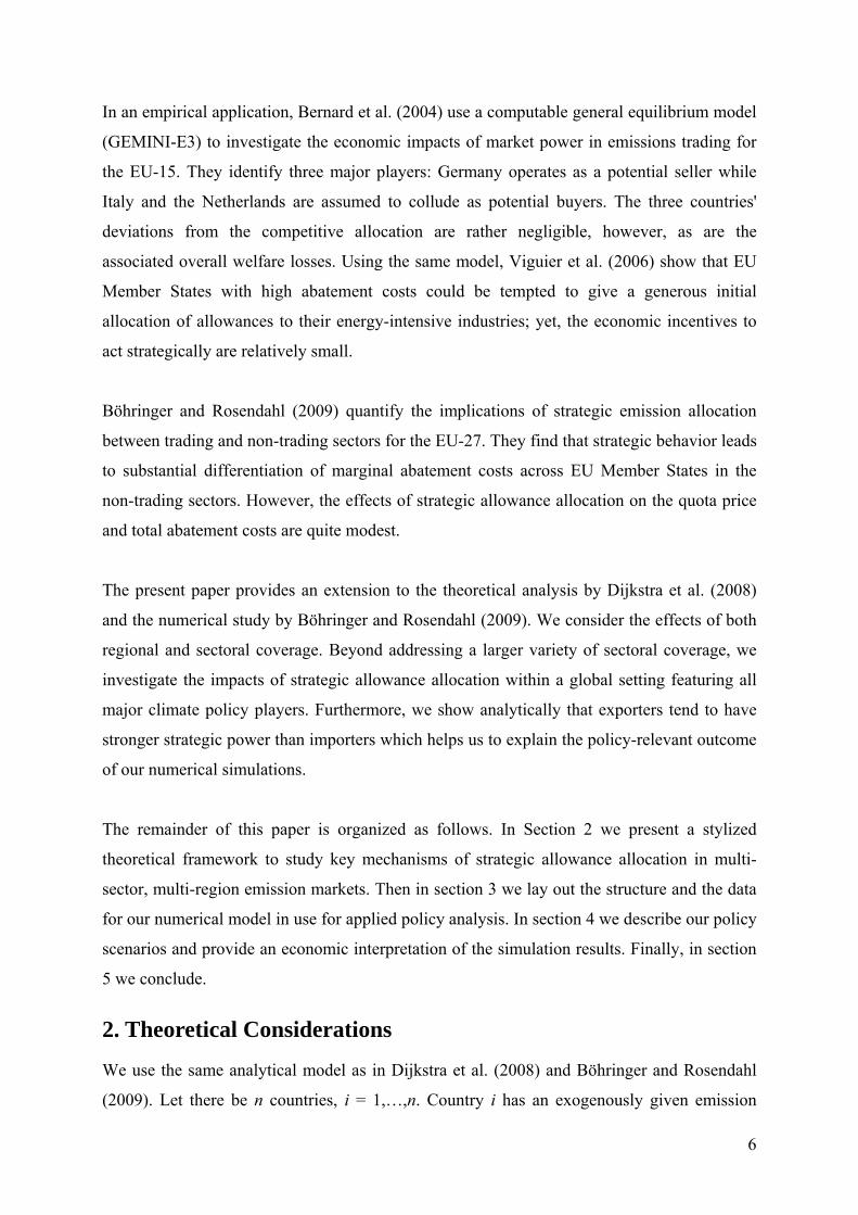
Figure 1 shows country i’s marginal abatement costs MCi,T as a function of emissions ei,T in
the trading segment, measured from left to right. Further, the figure shows the country’s
marginal abatement costs MCi,NT as a function of emissions ei,NT in the non-trading segment,
measured from right to left. The national ceiling is given by the distance OEi. Without
international trading, country i sets MCi,T = MCi,NT by (2), so that emissions in the trading
segment are ,NTRi Te and marginal costs in both segments are NTR
iP .
Figure 1: The switch from no international emissions trading to competitive trade
O
MC
MC
i,T
i,NT
ei,T ei,NTei,T
C qiC
PC
ei,TNTR
PNTR
Ei
With international emissions trading, country i's trading segment emissions ei,T will in general
differ from the emissions budget qi allocated to the trading segment by country i's emission
authority.6 The allocated emissions budget qi for the trading segment plus emissions ei,NT for
the non-trading segment must add up to the national ceiling Ei. After each country has set its
qi and distributed the permits among its trading segment, the polluters in the trading segments
trade the permits among each other. We assume that each individual polluter is too small to
have market power, and so each polluter takes the permit price P as given. Emissions ei,T are
then determined by:
, ,i T i TMC e P (3)
6 It makes no difference to our analysis whether the national government auctions or grandfathers the permits to its firms, or
(in the latter case) how it distributes the permits among its firms. This is because we assume the permit market is perfectly
competitive for firms, and because we are only interested in the welfare of the country as a whole.

9
under the restriction:
,1 1
n n
T j T jj j
e e q
(4)
That is, marginal abatement costs equal the permit price, and total emissions in all trading
segments equal the total amount of permits for the trading segments. Equations (3) and (4)
implicitly define P and ei,T as function of the total emissions eT in the trading segment with:
1, ,
1'( )
1
''
Tn
jj T j T
P e
C e
(5)
Country i now chooses qi to minimize overall abatement costs in the trading and non-trading
segments plus net expenditures on buying (selling) permits from (to) abroad:
, , , ,Min ( )i T i T i NT i i T i T iC e C E q P e e q (6)
Assuming an interior solution 0 < qi < 0,i Te ,7 the first-order condition, taking (3) into account,
is:
, , ,( ) ( ) '( ) ( )i NT i NT i i T T i T iMC e MR q P e P e e q (7)
where P'(eT) is given by (5) and MRi(qi) is country i’s marginal revenue of allocating more
permits to its trading segment. When country i is exporting permits, its marginal revenues are
below the international permit price (as for any seller with market power), because the extra
permits it allocates to its trading segment depress the price at which it can sell permits.
Correspondingly, when country i is importing permits, its marginal revenues exceed the
permit price.
Figures 1 and 2 illustrate how a country gains when it joins the international emissions trading
scheme. First consider the change from no international trading to competitive international
trade where country i takes the international permit price PC as given. This is illustrated in
Figure 1, where we have assumed CP > NTRiP . The country then minimizes overall costs by
setting its marginal costs in the non-trading segment equal to CP , as is clear from (7) with P'
7 In the numerical simulations (cf. section 4) there is one occasion (Brazil in region coverage variant C4 and sector coverage
variant ELE) where qi = 0, as the optimal allocation is negative. Then marginal costs in the non-trading segment are above
the marginal revenue, and we have an inequality in (7). We assume that countries are not allowed to overallocate, i.e., to
allocate more allowances to the trading segment than their business-as-usual emissions in that segment (qi ≤ 0,i Te ).
However, this restriction is never binding in the numerical simulations.
10
= 0. Thus, it allocates Ciq permits to its trading segment and the rest ( C
i iE q ) to its non-trading
segment. Firms in country i’s trading segment trade permits and emit ,Ci Te themselves, which in
the Figure 1 is lower than Ciq since CP > NTR
iP . Compared to the case without international
emissions trading, country i’s total costs have decreased by the shaded triangle above the MC-
curves and below the CP -line, i.e., export revenues minus increased abatement costs.
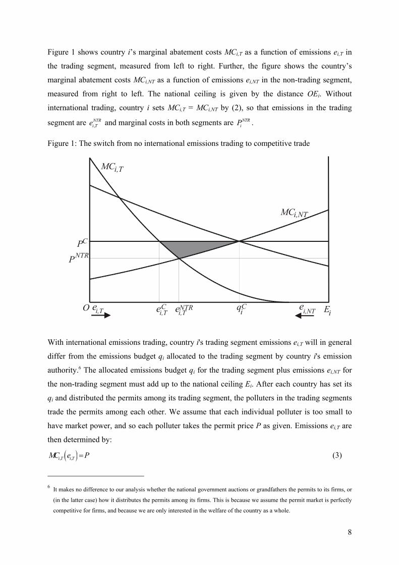
Figure 2: The switch from competitive trade to trade with market power
O
MC
MC
P(q )
MR (q )
i,T
i,NT
ei,T
i i
i
ei,T ei,TM C q
iM q
iC
P
P
M
C
ei,NT Ei
Figure 2 illustrates the switch from competitive trade to trade with market power.8 As before,
the international permit price will be CP if the country issues Ciq permits to its trading
segment. However, the permit price is now a decreasing function P(qi) of qi. Country i’s
marginal revenue MRi(qi) curve is located below (above) P(qi) when it is exporting
(importing) permits. We know from (7) that country i will set its marginal abatement costs in
the non-trading segment equal to the marginal revenues from selling permits (or buying less
permits) in the international market. It thus reduces its permit allocation to the trading
segment to Miq , driving the permit price up to MP in Figure 2. The trading segment will now
emit ,Mi Te , whereas the non-trading segment increases its emissions to (Ei – M
iq ). The cost
8 We assume throughout that all reaction curves are downward sloping (i.e., dqi /dqj < 0 for all i,j), and that there is a stable
and unique Nash equilibrium.
11
reduction compared to competitive behavior is the difference between the light-shaded
quadrangle and the dark-shaded triangle. The quadrangle represents the gain from selling
permits at a higher price. The triangle represents the efficiency loss from the domestic
distortion of letting MCi,NT deviate from the permit price.9
So far we have illustrated that a country gains when joining the international emissions
trading scheme while taking the permit price as given, and that there is an additional gain
should it be able to influence the permit price. It is easily seen that the costs of all
participating countries together are minimized when all sectors are included in the
international trading scheme.10 In this case there is no scope for countries to manipulate the
permit price by letting marginal cost in their non-trading segment deviate from the
international permit price.
However, a country will not necessarily benefit from the inclusion of additional sectors into
the international trading scheme. The discussion of Figure 2 indicates that the permit price for
strategic allowance allocation in general will deviate from the cost-effective solution as long
as the trading scheme only covers a subset of all sectors. Including more and more sectors into
the trading segment changes a country’s ability to manipulate the permit price. If a country
sees the permit price move in an adverse direction (up for a net importer, down for a net
exporter), its loss from this price change may dominate the gain from increased where-
flexibility, so that overall the country may lose from the sectoral expansion of the trading
scheme.
A country’s ability to manipulate the permit price depends on the slope of its marginal
abatement cost curve for the non-trading segment. Consider the marginal cost curve for the
non-trading segment, MCi,NT, in Figure 2. This curve is rather flat. Suppose that country i had
a much steeper MCi,NT curve which likewise intersects the P(qi) curve at Ciq . The country
would still issue Ciq permits to the trading segment if it took the permit price CP as given.
However, its domestic efficiency loss (i.e., the shaded triangle) from reducing the number of
9 Obviously, strategic allowance allocation provides additional cost savings for the joining country compared to competitive
behaviour, i.e., the difference between the light-shaded quadrangle and the dark-shaded triangle must be positive.
10 We abstract from transaction costs which may be prohibitively high for the large group of small polluters. Betz et al.
(2010) discuss the optimal coverage of the EU ETS, taking transaction costs into account.

12
permits to the trading segment to Miq would now be larger. Thus, the country would go less
far in reducing the number of permits in order to drive up the permit price, and so the dark-
shaded quadrangle would decrease. Thus, the flatter a country’s marginal abatement cost
curve in the non-trading segment is, the stronger is the incentive to manipulate the permit
price.11 If an expansion of the trading scheme makes a country’s marginal abatement costs in
the remaining non-trading segment much steeper, i.e., less elastic, this country will lose its
ability to manipulate the permit price in its favor and may see its overall costs increase as a
result of the expansion.
Before turning to the numerical analysis, let us briefly summarize what results we may expect
based on the theoretical discussion so far. First, we should expect larger countries to have
stronger impacts on the permit price than smaller countries. A large country would typically
have a larger volume of net trade and therefore a larger benefit from a permit price change.
Second, we laid out that a country’s incentive to manipulate the international permit price
increases with the flatness of the marginal abatement cost curve in its non-trading segment.
Furthermore, we should expect exporters to have more strategic power than importers, given
that marginal abatement costs are strictly convex.12 That is, the permit price will tend to be
above the competitive or cost-effective permit price as long as sectoral coverage is partial.
Formally, we can state:
Proposition:
Consider n countries with different national emissions targets, having a common trading
scheme that covers a subset of all sectors. Assume that countries freely decide on their permit
allocation, and play Nash in the allocation game. Assume also that marginal abatement cost
curves in the non-trading sectors are convex and identical across countries. Then the
emissions price in the trading scheme will be above the cost-effective emissions price level.
11 A flat marginal cost curve implies only a small cost of letting the permit allocation deviate from the point where marginal
costs equal the permit price.
12 In our quantitative analysis based on empirical data the aggregate marginal abatement cost functions for the non-trading
segment is always strictly convex for any country.
13
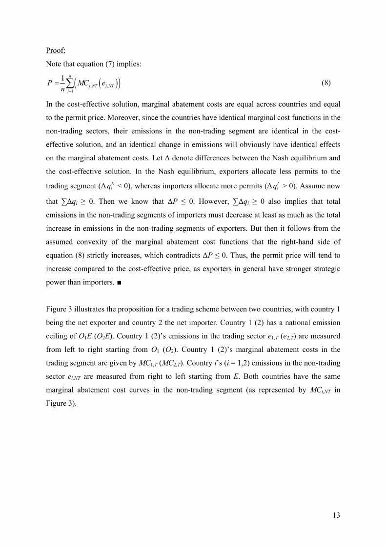
Proof:
Note that equation (7) implies:
, ,1
1 n
j NT j NTj
P MC en
(8)
In the cost-effective solution, marginal abatement costs are equal across countries and equal
to the permit price. Moreover, since the countries have identical marginal cost functions in the
non-trading sectors, their emissions in the non-trading segment are identical in the cost-
effective solution, and an identical change in emissions will obviously have identical effects
on the marginal abatement costs. Let Δ denote differences between the Nash equilibrium and
the cost-effective solution. In the Nash equilibrium, exporters allocate less permits to the
trading segment (Δ Eiq < 0), whereas importers allocate more permits (Δ I
iq > 0). Assume now
that ∑Δqi ≥ 0. Then we know that ΔP ≤ 0. However, ∑Δqi ≥ 0 also implies that total
emissions in the non-trading segments of importers must decrease at least as much as the total
increase in emissions in the non-trading segments of exporters. But then it follows from the
assumed convexity of the marginal abatement cost functions that the right-hand side of
equation (8) strictly increases, which contradicts ΔP ≤ 0. Thus, the permit price will tend to
increase compared to the cost-effective price, as exporters in general have stronger strategic
power than importers. ■
Figure 3 illustrates the proposition for a trading scheme between two countries, with country 1
being the net exporter and country 2 the net importer. Country 1 (2) has a national emission
ceiling of O1E (O2E). Country 1 (2)’s emissions in the trading sector e1,T (e2,T) are measured
from left to right starting from O1 (O2). Country 1 (2)’s marginal abatement costs in the
trading segment are given by MC1,T (MC2,T). Country i’s (i = 1,2) emissions in the non-trading
sector ei,NT are measured from right to left starting from E. Both countries have the same
marginal abatement cost curves in the non-trading segment (as represented by MCi,NT in
Figure 3).
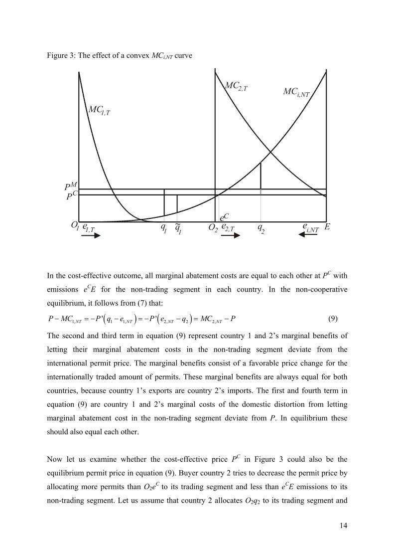
14
Figure 3: The effect of a convex MCi,NT curve
In the cost-effective outcome, all marginal abatement costs are equal to each other at PC with
emissions eCE for the non-trading segment in each country. In the non-cooperative
equilibrium, it follows from (7) that:
1, 1 1, 2, 2 2,' 'NT NT NT NTP MC P q e P e q MC P (9)
The second and third term in equation (9) represent country 1 and 2’s marginal benefits of
letting their marginal abatement costs in the non-trading segment deviate from the
international permit price. The marginal benefits consist of a favorable price change for the
internationally traded amount of permits. These marginal benefits are always equal for both
countries, because country 1’s exports are country 2’s imports. The first and fourth term in
equation (9) are country 1 and 2’s marginal costs of the domestic distortion from letting
marginal abatement cost in the non-trading segment deviate from P. In equilibrium these
should also equal each other.
Now let us examine whether the cost-effective price PC in Figure 3 could also be the
equilibrium permit price in equation (9). Buyer country 2 tries to decrease the permit price by
allocating more permits than O2eC to its trading segment and less than eCE emissions to its
non-trading segment. Let us assume that country 2 allocates O2q2 to its trading segment and
15
q2E to its non-trading segment. Then to keep the permit price at PC, country 1 would have to
allocate 11~qO to its trading segment and Eq1
~ to its non-trading segment. This is because the
distance Ceq1~
equals 2qeC , so that the total amount allocated to the non-trading segment (and
thereby the total amount allocated to the trading segment) remains the same. However, the
gap between the permit price PC and the marginal abatement cost MCi,NT is now much smaller
for country 1 than for country 2,13 because the MCi,NT curve is strictly convex. According to
equation (9), these gaps, which measure the marginal costs of the domestic distortion, should
be the same for both countries. Hence, exporting country 1 will further restrict its permit
allocation to the trading segment. In equilibrium, country 1 allocates O1q1 to its trading sector
and q1E to its non-trading sector, while country 2 allocates O2q2 and q2E respectively. Total
emissions in the trading segment are lower than in the cost-effective outcome, so that the
permit price is now PM, which exceeds the cost-effective price PC. The two countries then
have the same gap between the permit price PM and the marginal abatement cost MCi,NT, i.e.,
equal marginal costs of domestic distortion, as required by (9).14
3. Numerical Model and Benchmark Data
In order to investigate the prospects for expanding the EU ETS towards a more
comprehensive coverage of sectors and regions we make use of a numerical carbon market
model. The model is based on marginal abatement cost curves which reflect differences in
emission reduction possibilities across sectors and regions. We can generate these cost
functions in continuous form given a sufficiently large number of discrete observations for
marginal abatement costs and the induced emission reductions in sectors and regions. In
applied research marginal abatement costs are often provided as discrete step-functions where
the data is either collected through expert assessments of abatement possibilities or generated
through bottom-up models of the energy system (e.g., Criqui and Mima, 2001; Capros et al.,
1998). Another wide-spread method is to derive marginal abatement costs curves from
economy-wide models with a top-down representation of emission reduction possibilities in
production and consumption (see, e.g., Eyckmans et al., 2001).
13 In Figure 3, the gaps are given by the dark thick vertical line above
1~q for country 1 and the grey plus the dark thick
vertical lines above q2 for country 2.
14 The gap between the international permit price and marginal abatement cost in the non-trading segment is given by the
dark thick vertical lines above q1 and q2 respectively.
16
As our numerical analysis requires marginal abatement cost curves for many sectors and
regions, a bottom-up approach is not practical. We therefore employ an established multi-
sector, multi-region computable general equilibrium (CGE) model of the world economy (see
Böhringer and Rutherford, 2010, for a recent detailed model description) to obtain explicit
reduced-form representations of marginal abatement cost curves. The CGE model is based on
the GTAP7 dataset for 2004 which features consistent accounts of production and
consumption, bilateral trade and energy (carbon emission) flows for 57 sectors and 113
regions (Badri and Walmsley, 2008) and is complemented with econometric estimates on
sector-specific elasticities of substitution (Okagawa and Ban, 2008). Since our numerical
simulations refer to 2020 as the central compliance year for a potential Post-Kyoto agreement,
we perform a business-as-usual forward projection of the model to 2020 based on information
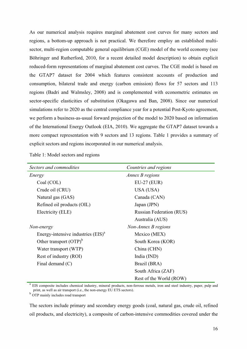
of the International Energy Outlook (EIA, 2010). We aggregate the GTAP7 dataset towards a
more compact representation with 9 sectors and 13 regions. Table 1 provides a summary of
explicit sectors and regions incorporated in our numerical analysis.
Table 1: Model sectors and regions
Sectors and commodities Countries and regions
Energy Annex B regions
Coal (COL) EU-27 (EUR)
Crude oil (CRU) USA (USA)
Natural gas (GAS) Canada (CAN)
Refined oil products (OIL) Japan (JPN)
Electricity (ELE) Russian Federation (RUS)
Australia (AUS)
Non-energy Non-Annex B regions
Energy-intensive industries (EIS)a Mexico (MEX)
Other transport (OTP)b South Korea (KOR)
Water transport (WTP) China (CHN)
Rest of industry (ROI) India (IND)
Final demand (C) Brazil (BRA)
South Africa (ZAF)
Rest of the World (ROW) a EIS composite includes chemical industry, mineral products, non-ferrous metals, iron and steel industry, paper, pulp and
print, as well as air transport (i.e., the non-energy EU ETS sectors). b OTP mainly includes road transport
The sectors include primary and secondary energy goods (coal, natural gas, crude oil, refined
oil products, and electricity), a composite of carbon-intensive commodities covered under the

17
existing EU ETS, and important candidates for sectoral expansion, in particular transport
activities. The remaining production of commodities and services is summarized in one
aggregate sector; likewise private consumption patterns with associated carbon emissions are
reflected in a composite final demand activity. The regions depicted for our analysis represent
key players in the climate policy debate which may be seen as potential candidates for linking
up with the EU ETS.
For the sectors and regions listed in Table 1 we generate marginal abatement cost functions
through a sequence of hypothetical tax scenarios where we impose sector- and region-specific
CO2 taxes starting from $0 to $100 per ton of CO2 in steps of $1 and then read off the CGE
solution for the induced emission reduction. We then perform a least-square fit by a
polynomial marginal abatement cost function of third degree to the set of “observations”:
0 0 2 0 3, , , , , , , , , , ,( ) 1 ( ) 2 ( ) 3 ( ) i s i s i s i s i s i s i s i s i s i s i sMC e a e e a e e a e e
(10)
where
, ,( )i s i sMC e denotes the marginal abatement cost of sector s in region i,
0,i se is the business-as-usual emission level of sector s in region i,
,i se is the emission level of sector s in region i at a CO2 price equal to
, ,( )i s i sMC e , and
,1i sa , ,2i sa , ,3i sa are the fitted coefficients in the marginal abatement cost function of
sector s in region i.
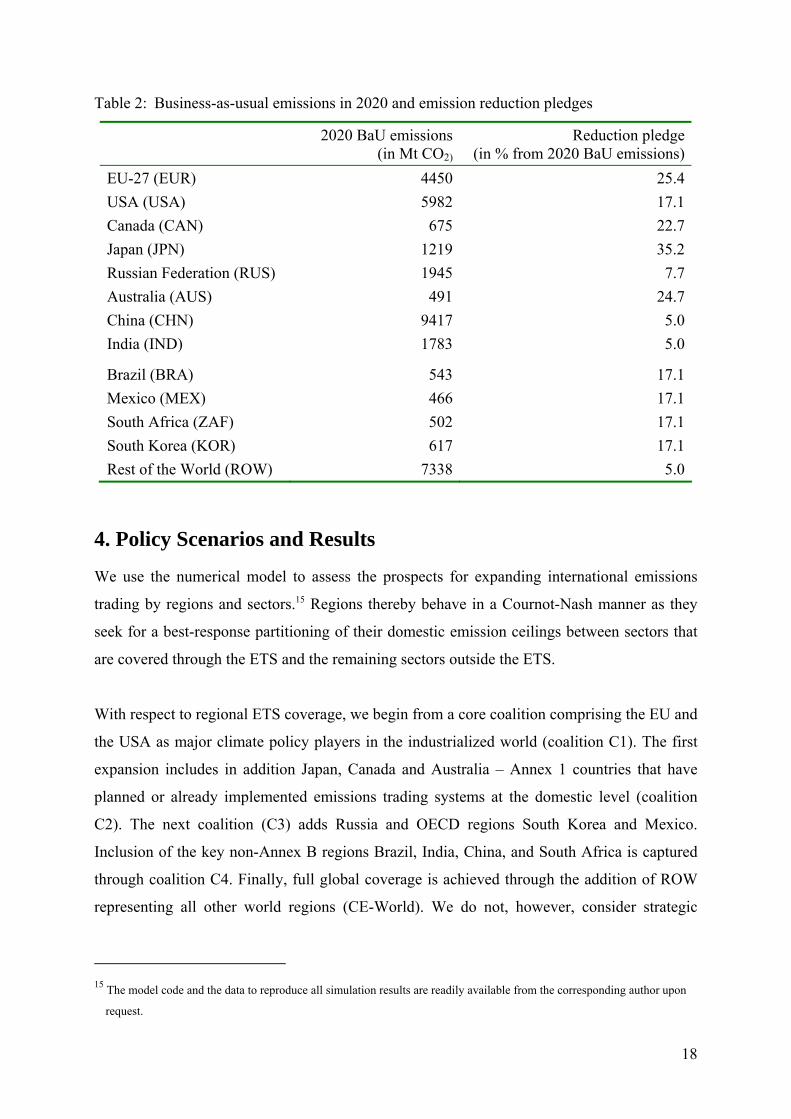
Table 2 details projected business-as-usual (BaU) CO2 emissions in 2020 together with
emission reduction targets from 2020 BaU levels across model regions. We have derived the
post-Kyoto reduction pledges for 2020 from national communications following the
Copenhagen Accord (UNFCCC, 2009), of which the 15th Conference of Parties to the United
Nations Framework Convention on Climate Change “took note”. The Copenhagen Accord
requested Annex I countries to submit their “quantified economy-wide targets for 2020” and
the non-Annex I countries to announce their “nationally appropriate mitigating actions”. All
major economies of the world had submitted their pledges by spring 2010. The Appendix
provides a detailed explanation on how we derived emission reductions targets for our model
regions based on national communications to the Copenhagen Accord.
18
Table 2: Business-as-usual emissions in 2020 and emission reduction pledges
2020 BaU emissions (in Mt CO2)
Reduction pledge (in % from 2020 BaU emissions)
EU-27 (EUR) 4450 25.4
USA (USA) 5982 17.1
Canada (CAN) 675 22.7
Japan (JPN) 1219 35.2
Russian Federation (RUS) 1945 7.7
Australia (AUS) 491 24.7
China (CHN) 9417 5.0
India (IND) 1783 5.0
Brazil (BRA) 543 17.1
Mexico (MEX) 466 17.1
South Africa (ZAF) 502 17.1
South Korea (KOR) 617 17.1
Rest of the World (ROW) 7338 5.0
4. Policy Scenarios and Results
We use the numerical model to assess the prospects for expanding international emissions
trading by regions and sectors.15 Regions thereby behave in a Cournot-Nash manner as they
seek for a best-response partitioning of their domestic emission ceilings between sectors that
are covered through the ETS and the remaining sectors outside the ETS.
With respect to regional ETS coverage, we begin from a core coalition comprising the EU and
the USA as major climate policy players in the industrialized world (coalition C1). The first
expansion includes in addition Japan, Canada and Australia – Annex 1 countries that have
planned or already implemented emissions trading systems at the domestic level (coalition
C2). The next coalition (C3) adds Russia and OECD regions South Korea and Mexico.
Inclusion of the key non-Annex B regions Brazil, India, China, and South Africa is captured
through coalition C4. Finally, full global coverage is achieved through the addition of ROW
representing all other world regions (CE-World). We do not, however, consider strategic
15 The model code and the data to reproduce all simulation results are readily available from the corresponding author upon
request.

19
behavior by ROW, accounting for the heterogeneity and the large number of embodied
countries.
With respect to sectoral ETS coverage, we first consider the extreme case that no sector is
included in the ETS. This setting is equivalent to exclusively domestic abatement without
international emissions trading. In the next step (ELE) the power generation sector, which is
by far the most important source of CO2 emissions across all countries, can trade emission
allowances internationally. Variant EIS adds the other energy sectors and all energy-intensive
industries to the ETS reflecting the current coverage of the ETS in Europe (i.e., sectors COL,
CRU, GAS, OIL and EIS in Table 1). We then sequentially add CO2-intensive transport
sectors (variants OTP and WTP) to the ETS, and furthermore consider the rest of industry
(ROI) as a segment to be added to the ETS. The final addition to the ETS is made through
final demand (variant C) which results in full coverage of domestic emissions by the ETS. In
this variant C there is no possibility to undertake strategic partitioning and we thus obtain the
outcome of competitive emissions trading.
Table 3: Regional and sectoral coverage of international emissions trading scenarios
Regional coverage (coalitions) Sectoral coveragea
No trade None None
C1 EU-27 + USA ELE ELE
C2 C1 +
(Japan, Canada, Australia)
EIS ELE +
COL, CRU, GAS, OIL, EIS
C3 C2 +
(Russia, South Korea, Mexico)
OTP EIS +
OTP
C4 C3 +
(China, India, Brazil, South Africa)
WTP OTP +
WTP
CE-World All regions ROI WTP +
ROI
C ROI +
C a The variants of sectoral coverage are written in italics (e.g., OTP), whereas sectors are not (e.g., OTP). For
instance, variant OTP comprises several sectors, where the OTP sector is the additional sector included in the ETS under this variant. Sectors are defined in Table 1.
Table 3 summarizes the dimensionalities of (international) emissions trading scenarios with
respect to regional and sectoral coverage. The sequence of expanding trading by sectors and
regions is motivated by our view of a pragmatic climate policy course. Clearly, the numerical

20
results for individual countries are dependent on this sequence but – as will follow from our
interpretation below – the more general economic insights will still prevail.
We report the implications of regional and sectoral expansion with respect to a no-trading
scenario where each region complies with its specific emission reduction pledge through a
domestic economy-wide CO2 tax or likewise a comprehensive domestic cap-and-trade system
without international emissions trading (this reference scenario corresponds to the settings
“none” for regional coverage and “none” for sectoral coverage in Table 3 above).16
Let us first consider the effects of regional expansion. Figure 4 shows how the costs of
complying with the national target are reduced vis-à-vis the no-trading case when a country is
part of a coalition, and how these cost reductions change as the coalition expands. Sectoral
coverage is then kept constant at variant EIS which reflects the actual coverage of the EU
ETS. We see for instance that U.S. costs are reduced by 20% when joining a coalition with
the EU (C1), with the cost reduction growing to 53% when Canada, Japan and Australia are
also included (C2). However, when even more countries are included, U.S. compliance costs
start to increase, and in the largest coalition there are only rather modest gains vis-à-vis the
autarky for the USA. The reasoning behind is that the quota price changes depending on who
is part of the coalition – if the quota price then becomes close to the autarky quota price, there
is little to gain from external trade.
Note that Russia, China and India see their costs turn into a net gain when they join the
international emissions trading scheme since the revenues from permit exports more than
offset their abatement costs. The cost reductions for these countries in Figures 4, 7 and 8 are
measured along the right-hand axis (RH). For instance, the cost reduction of 1800% for
Russia under coalition C3 means that the abatement costs without international emissions
trading have turned into a gain that is 17 times as large as the original costs (note that the
latter are rather small).
16 For the no-trading benchmark scenario the CO2 taxes, quota prices or likewise marginal abatement costs amount to (in
USD per ton of CO2): EUR 75.5, USA 25.9, CAN 57.4, JPN 326.8, RUS 5.9, AUS 41.3, CHN 4.2, IND 4.7, BRA 95.7,
MEX 48.5, ZAF 8.5, KOR 30.4, and ROW 5.4.

21
Figure 4: Accumulated cost reductions by expanding the coalition (variant EIS)
0 %
10 %
20 %
30 %
40 %
50 %
60 %
70 %
80 %
90 %
C1 C2 C3 C4 CE-World
0 %
200 %
400 %
600 %
800 %
1000 %
1200 %
1400 %
1600 %
1800 %
2000 %
EUR USA CAN JPN AUS BRAKOR MEX ZAF RUS (RH) CHN (RH) IND (RH)
Figure 4 also illustrates that there will be opposite interests among current coalition members
whether to invite new countries into the coalition or not. Again, this is related to the direction
in which the quota price will change, and which countries are importers and which are
exporters. For instance, the USA (exporter of quotas) will oppose new members after Canada,
Japan and Australia are included, because this would drive down the quota price, whereas the
other countries (importers of quotas) would like to include new members. Thus, it may be
difficult to agree upon an expansion of the ETS in the direction of new coalition members.
Figures 5 through 8 show – for a given coalition – how the costs are reduced when going from
no-trading to international permit trading between electricity sectors only, and then further
expanding the sectoral coverage of the ETS. First, we see that the biggest cost reductions
already occur when opening for permit trade through a sufficiently large emission-intensive
sector such as the electricity sector (variant ELE). Nevertheless, there are still some cost
reductions to be gained from expansion towards full coverage (C), indicating that there is
some non-negligible strategic behavior. Aggregate costs are reduced by respectively 4%, 4%,
2% and 10% in coalitions C1, C2, C3 and C4 when going from ELE to full coverage. For
individual countries such as Japan and Brazil, the cost reductions are even higher (16% and
19% in C4).

22
Although cost savings usually increase with coverage, it is possible for countries to lose from
sectoral expansion of the trading scheme, as pointed out in Section 2. For instance, in
coalition C2, the USA loses when the two last sectors are added to the trading scheme
(variants ROI and C). In coalition C3, the USA is best off with either only the electricity
sector included (ELE) or with all sectors but final demand (variant ROI) included in the ETS.
Several countries achieve their largest cost reductions (or their highest overall gains) when
only ELE is included in the trading scheme. These are in particular Australia in coalition C2,
and Russia, China, India and South Africa in coalition C4.
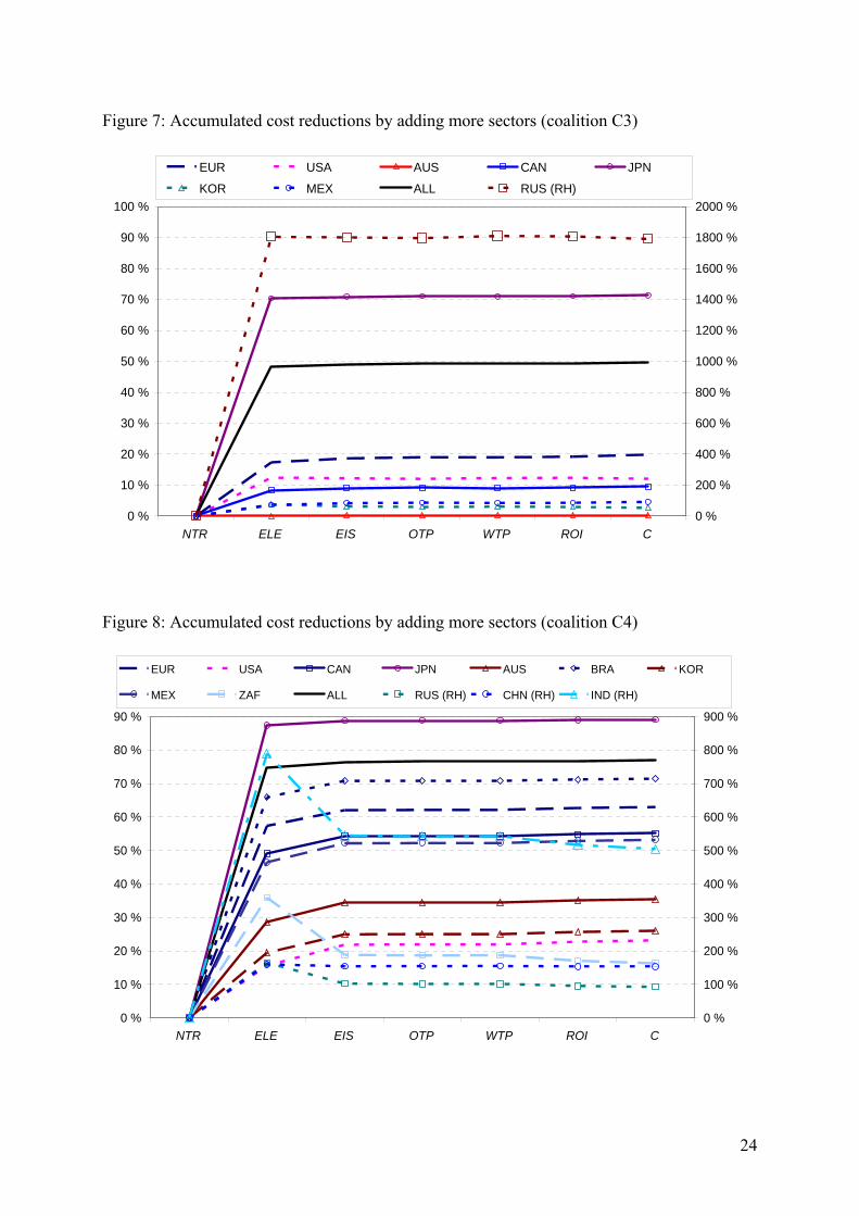
The impacts of sectoral expansion are generally largest when the coalition is small (the
strategic influence of a single country falls as the coalition expands). This is particularly
evident from the approximately horizontal curves in Figure 7 (coalition C3) to the right of
ELE. However, we notice some dramatic changes with the largest coalition in Figure 8,
especially when we expand the ETS from ELE to EIS. In order to explain this, remember that
China joins the coalition in C4. Chinese emissions are very large, with low abatement costs
and only modest cutbacks (see Table 2). Thus, China is a dominant supplier of permits in C4,
accounting for 77% of permit sales when all sectors are included in the ETS. Hence, the
country has significant strategic incentives to cut back on the sales of permits.
Further, China’s strategic power declines substantially when expanding from ELE to EIS. The
reasoning behind is that the energy-intensive sector in China has both large emissions and low
abatement costs which warrants significant strategic power for the case that the energy-
intensive sectors remain part of the non-trading segment (cf. section 2). As an indicator of
this, Chinese exports of permits under ELE account for 69% of permit sales (versus 75-77%
with more sectors included). We notice from Figure 8 that India, Russia and South Africa –
all the three being permit exporters – gain relatively more than China as they can free ride on
China’s export restraint which leads to relatively high permit price under ELE (see Figure 12
below). In absolute terms, however, China gains more than Russia and South Africa and
almost as much as India.

23
Figure 5: Accumulated cost reductions by adding more sectors (coalition C1)
0 %
5 %
10 %
15 %
20 %
25 %
NTR ELE EIS OTP WTP ROI C
EUR USA ALL
Figure 6: Accumulated cost reductions by adding more sectors (coalition C2)
0 %
10 %
20 %
30 %
40 %
50 %
60 %
70 %
NTR ELE EIS OTP WTP ROI C
EUR USA CAN JPN AUS ALL
24
Figure 7: Accumulated cost reductions by adding more sectors (coalition C3)
0 %
10 %
20 %
30 %
40 %
50 %
60 %
70 %
80 %
90 %
100 %
NTR ELE EIS OTP WTP ROI C
0 %
200 %
400 %
600 %
800 %
1000 %
1200 %
1400 %
1600 %
1800 %
2000 %
EUR USA AUS CAN JPN
KOR MEX ALL RUS (RH)
Figure 8: Accumulated cost reductions by adding more sectors (coalition C4)
0 %
10 %
20 %
30 %
40 %
50 %
60 %
70 %
80 %
90 %
NTR ELE EIS OTP WTP ROI C
0 %
100 %
200 %
300 %
400 %
500 %
600 %
700 %
800 %
900 %
EUR USA CAN JPN AUS BRA KOR
MEX ZAF ALL RUS (RH) CHN (RH) IND (RH)
25
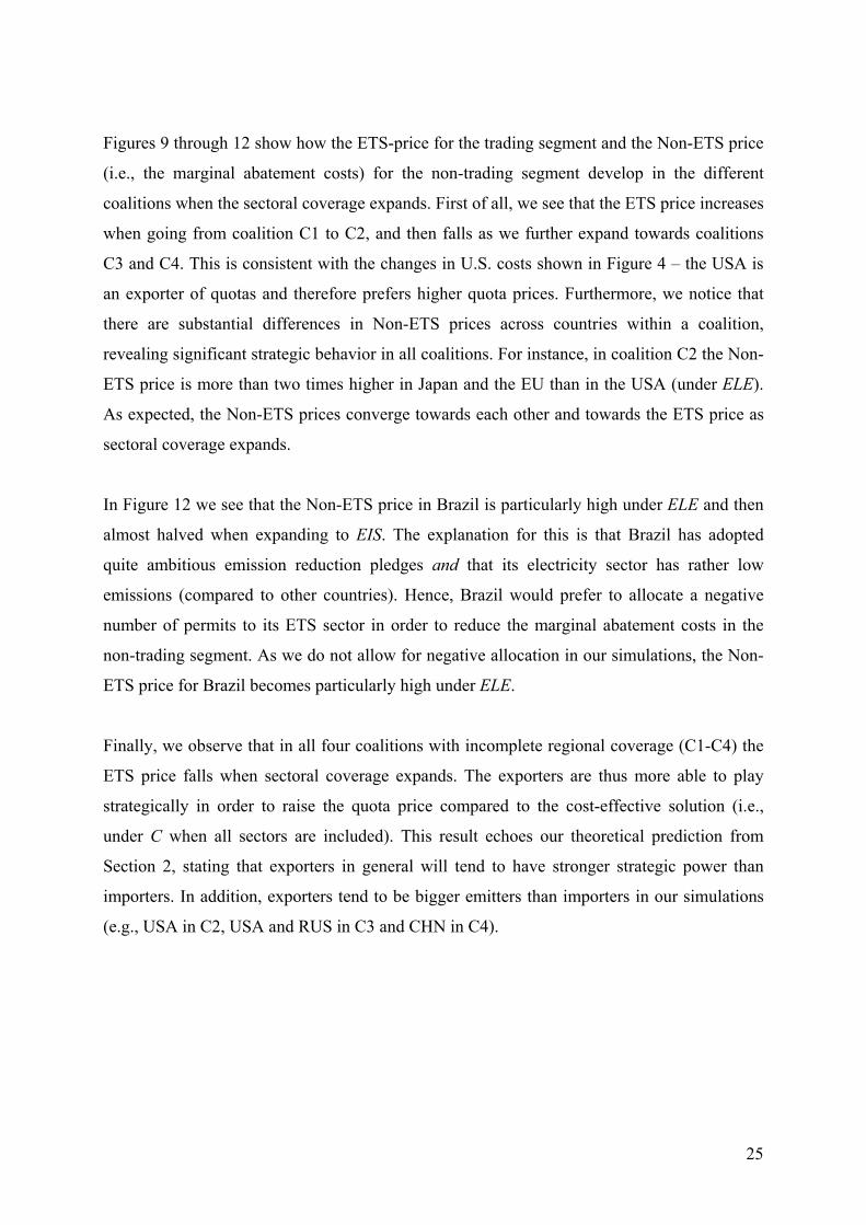
Figures 9 through 12 show how the ETS-price for the trading segment and the Non-ETS price
(i.e., the marginal abatement costs) for the non-trading segment develop in the different
coalitions when the sectoral coverage expands. First of all, we see that the ETS price increases
when going from coalition C1 to C2, and then falls as we further expand towards coalitions
C3 and C4. This is consistent with the changes in U.S. costs shown in Figure 4 – the USA is
an exporter of quotas and therefore prefers higher quota prices. Furthermore, we notice that
there are substantial differences in Non-ETS prices across countries within a coalition,
revealing significant strategic behavior in all coalitions. For instance, in coalition C2 the Non-
ETS price is more than two times higher in Japan and the EU than in the USA (under ELE).
As expected, the Non-ETS prices converge towards each other and towards the ETS price as
sectoral coverage expands.
In Figure 12 we see that the Non-ETS price in Brazil is particularly high under ELE and then
almost halved when expanding to EIS. The explanation for this is that Brazil has adopted
quite ambitious emission reduction pledges and that its electricity sector has rather low
emissions (compared to other countries). Hence, Brazil would prefer to allocate a negative
number of permits to its ETS sector in order to reduce the marginal abatement costs in the
non-trading segment. As we do not allow for negative allocation in our simulations, the Non-
ETS price for Brazil becomes particularly high under ELE.
Finally, we observe that in all four coalitions with incomplete regional coverage (C1-C4) the
ETS price falls when sectoral coverage expands. The exporters are thus more able to play
strategically in order to raise the quota price compared to the cost-effective solution (i.e.,
under C when all sectors are included). This result echoes our theoretical prediction from
Section 2, stating that exporters in general will tend to have stronger strategic power than
importers. In addition, exporters tend to be bigger emitters than importers in our simulations
(e.g., USA in C2, USA and RUS in C3 and CHN in C4).

26
Figure 9: Non-ETS prices and ETS price (coalition C1)
25
30
35
40
45
50
55
60
ELE EIS OTP WTP ROI C
EUR USA ETS
Figure 10: Non-ETS prices and ETS price (coalition C2)
30
35
40
45
50
55
60
65
70
75
ELE EIS OTP WTP ROI C
EUR USA AUS CAN JPN ETS

27
Figure 11: Non-ETS prices and ETS price (coalition C3)
20
25
30
35
40
45
50
ELE EIS OTP WTP ROI C
EUR USA AUS CAN JPN RUS ETS KOR MEX
Figure 12: Non-ETS prices and ETS price (C4)
5
7
9
11
13
15
17
19
21
23
ELE EIS OTP WTP ROI C
EUR USA AUS CAN JPN RUS KOR
MEX CHN IND BRA ZAF ETS
28
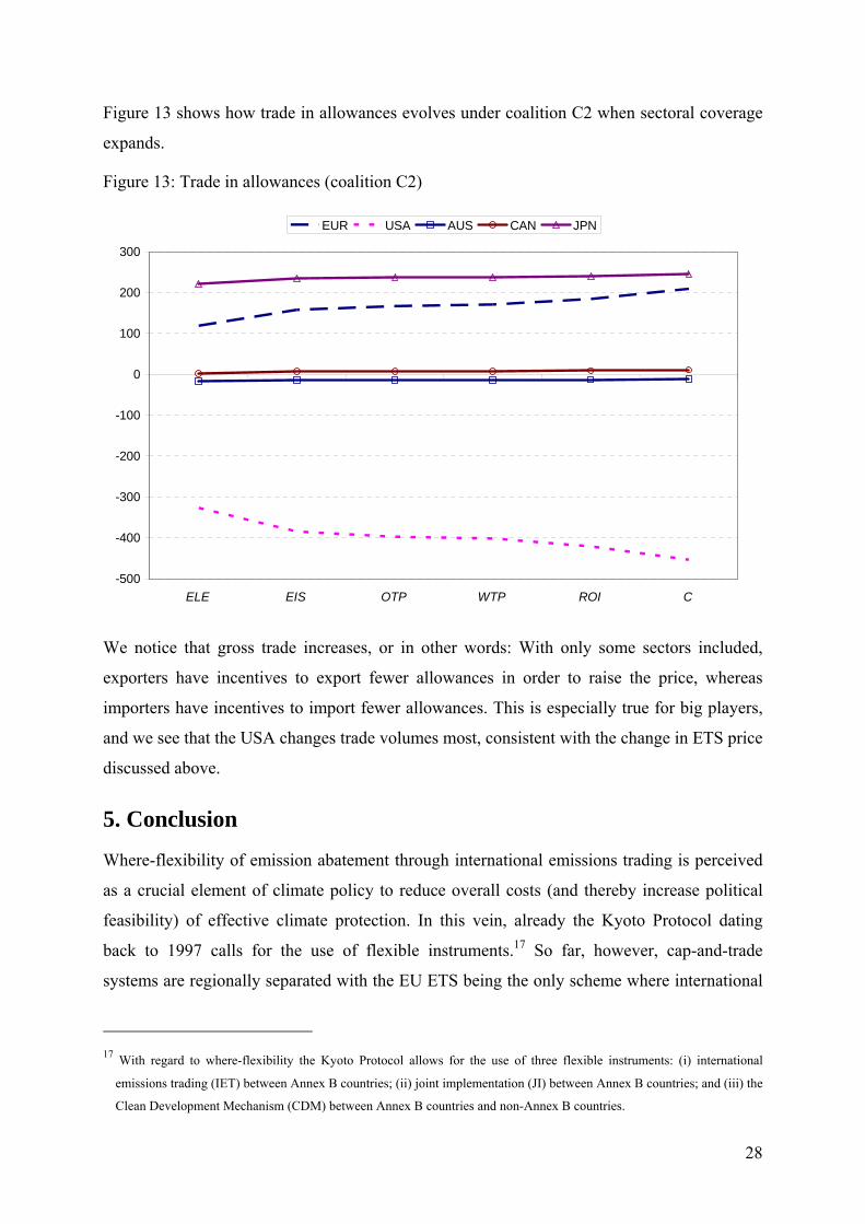
Figure 13 shows how trade in allowances evolves under coalition C2 when sectoral coverage
expands.
Figure 13: Trade in allowances (coalition C2)
-500
-400
-300
-200
-100
0
100
200
300
ELE EIS OTP WTP ROI C
EUR USA AUS CAN JPN
We notice that gross trade increases, or in other words: With only some sectors included,
exporters have incentives to export fewer allowances in order to raise the price, whereas
importers have incentives to import fewer allowances. This is especially true for big players,
and we see that the USA changes trade volumes most, consistent with the change in ETS price
discussed above.
5. Conclusion
Where-flexibility of emission abatement through international emissions trading is perceived
as a crucial element of climate policy to reduce overall costs (and thereby increase political
feasibility) of effective climate protection. In this vein, already the Kyoto Protocol dating
back to 1997 calls for the use of flexible instruments.17 So far, however, cap-and-trade
systems are regionally separated with the EU ETS being the only scheme where international
17 With regard to where-flexibility the Kyoto Protocol allows for the use of three flexible instruments: (i) international
emissions trading (IET) between Annex B countries; (ii) joint implementation (JI) between Annex B countries; and (iii) the
Clean Development Mechanism (CDM) between Annex B countries and non-Annex B countries.
29
emissions trading takes place across multiple jurisdictions. Apart from limited regional
coverage, trading schemes are in general also restricted to energy-intensive industries in terms
of sectoral coverage. As a prime example the EU ETS covers only around 40% of overall EU
greenhouse gas emissions.
Given the limitations in regional and sectoral coverage of actual trading schemes there is
broad consensus among climate policy makers to push for increased coverage in order to
exploit the cost savings potentials of comprehensive where-flexibility. Yet, the feasibility of
overall cost savings might be seriously hampered through opposed incentives from the
perspective of individual countries.
In this paper we have investigated the economic implications of regional and sectoral
expansion of international emissions trading in a policy setting where individual countries are
bound to emission reduction pledges under the Copenhagen Accords but incomplete sectoral
coverage provides scope for strategic behavior to manipulate the international emission price.
With our integrated theoretical and applied analysis we shed some light on the economic
incentives at stake when climate policy makers contemplate the regional linkage and sectoral
expansion of emission trading regimes.
As to regional expansion our results illustrate that the interests of quota exporters and
importers are usually opposed when including more countries into the trading scheme. The
exporters would like to let in more potential importers, which would raise the quota price,
while the importers would like to let in more potential exporters to depress the quota price.
When expanding sectoral coverage for a given trading coalition of countries, the highest cost
reductions generally come from the first step: going from “No trade” to a trading scheme that
includes one sector with a sufficiently large emission share (in our case: the electricity sector).
When sectoral coverage is expanded, a country usually gains, however we identify several
cases in our numerical simulations where countries lose. This happens because sectoral
expansion makes the marginal abatement costs in the remaining non-trading segment of these
countries less elastic, so that they are less able to manipulate the quota price in their preferred
direction. The USA and Russia are the countries that most frequently experience a loss from
sectoral expansion of the trading scheme.
30
The economic impacts of sectoral expansion are more substantial when the coalition is small,
because an individual country has more market power in a smaller coalition. However,
including China into the coalition means that a particularly large player joins the carbon
market, implying significant strategic effects if the trading scheme only covers the electricity
sector. Sectoral expansion reduces the quota price in all our simulations, consistent with our
theoretical prediction. This implies that – as a group – exporters have more market power than
importers, but their influence decreases when more sectors are added to the scheme.
References
Babiker, M., J. Reilly and L. Viguier (2004), “Is international emission trading always
beneficial?”, Energy Journal 25(2): 33-56.
Badri, N. G. and T. L. Walmsley (eds.) (2008), “Global Trade, Assistance and Production:
The GTAP 7 Data Base”, Center for Global Trade Analysis, Purdue University.
Bernard, A., M. Vielle, and L. Viguier (2004), “Modeling the European Directive establishing
a scheme for greenhouse gas allowance trading and assessing the market power of firms”,
REME working paper, École Polytechnique Fédérale Lausanne.
Betz, R., T. Sanderson and T. Ancev (2010), “In or out: efficient inclusion of installations in
an emissions trading scheme?”, Journal of Regulatory Economics 37: 162-179.
Bhagwati, J.N., A. Panagariya and T.N. Srinivasan (1998), Lectures on International Trade,
Second Edition, MIT Press, Cambridge (Mass.).
Böhringer, C., T. Hoffmann, A. Lange, A. Löschel and U. Moslener (2005), “Assessing
Emission Allocation in Europe: An Interactive Simulation Approach”, Energy Journal
26(4): 1-22.
Böhringer, C., H. Koschel and U. Moslener (2008), “Efficiency losses from overlapping
regulation of EU carbon emissions”, Journal of Regulatory Economics 33: 299-317.
Böhringer, C. and K.E. Rosendahl (2009), “Strategic Partitioning of Emissions Allowances
under the EU Emissions Trading Scheme”, Resource and Energy Economics 31: 182–197.
Böhringer, C. and T.F. Rutherford (2010), “The Costs of Compliance: A CGE Assessment of
Canada’s Policy Options under the Kyoto Protocol”, The World Economy 33: 177-211.

31
Capros, P., L. Mantzos, D. Kolokotsas, N. Ioannou, T. Georgakopoulos, A. Filippopoulitis
and Y. Antoniou (1998), “The PRIMES energy system model – reference manual”,
National Technical University of Athens, document as peer reviewed by the European
Commission, Directorate General for Research.
Convery, F.J. (2009), “Origins and Development of the EU ETS”, Environmental and
Resource Economics 43: 391-412.
Criqui, P. and S. Mima (2001), “The European greenhouse gas tradable emission permit
system: some policy issues identified with the POLES-ASPEN model”, ENER Bulletin 23:
51-55.
Dijkstra, B.R., E. Manderson and T-Y. Lee (2008), “Partial international emissions trading”,
GEP Research Paper 2008/27, University of Nottingham.
Dijkstra, B.R., E. Manderson and T-Y. Lee (2011), “Extending the sectoral coverage of an
international emissions trading scheme”, forthcoming in Environmental and Resource
Economics.
EIA (2009), “International Energy Outlook”, Energy Information Administration, US
Department of Energy, available at http://www.eia.doe.gov/oiaf/ieo/.
EIA (2010), “International Energy Outlook”, Energy Information Administration, US
Department of Energy, available at http://www.eia.doe.gov/oiaf/ieo/.
Eichner, T. and R. Pethig (2009), “Efficient CO2 emissions control with emissions taxes and
international emissions trading”, European Economic Review 53: 625-635.
Eyckmans, J., D. van Regemorter and V. van Steenberghe (2001): “Is Kyoto fatally flawed? –
An Analysis with MacGEM”, Working Paper Series - Faculty of Economics, University of
Leuven, No. 2001-18, Leuven.
EU (2007), “Limiting Global Climate Change to 2 degrees Celsius – The way ahead for 2020
and beyond”, European Commission, Brussels; available at:
http://ec.europa.eu/environment/climat/future_action.htm
Godal, O. and B. Holtsmark (2010), “International emissions trading with endogenous taxes”,
Discussion Papers 626, Statistics Norway.
Helm, C. (2003), “International emissions trading with endogenous allowance choices”,
Journal of Public Economics 87: 2737-2747.
32
Kruger, J.K. and W.A. Pizer (2004), “Greenhouse gas trading in Europe: the grand new policy
experiment”, Environment 46: 8-23.
Maeda, A. (2003), “The emergence of market power in emission rights markets: The role of
initial permit distribution”, Journal of Regulatory Economics 24: 293-314.
Malueg, D.A. and A.J. Yates (2009a), “Bilateral oligopoly, private information, and pollution
permit markets”, Environmental and Resource Economics 43: 553-572.
Malueg, D.A. and A.J. Yates (2009b), “Strategic behaviour, private information, and
decentralisation in the European Union Emissions Trading Scheme”, Environmental and
Resource Economics 43: 413-432.
Okagawa, A. and K. Ban (2008), “Estimation of Substitution Elasticities for CGE Models”,
mimeo, Osaka University, April 2008, available at:
http://www.esri.go.jp/jp/workshop/080225/03_report5_Okagawa.pdf
Schüle, R. and W. Sterk (2009), “Linking domestic emissions trading schemes and the
evolution of the international climate regime bottom-up support of top-down processes?”,
Introduction to the special issue, Mitigation and Adaptation Strategies for Global Change
375-378, DOI: 10.1007/s11027-009-9182-9
Viguier, L., M. Vielle, A. Haurie, A. Bernard (2006), “A two-level computable equilibrium
model to assess the strategic allocation of emission allowances within the European
Union”, Computers and Operations Research 33: 369–385.
Westskog, H. (1996), “Market power in a system of tradeable CO2 quotas”, Energy Journal
17(3): 85-103.
33
Appendix: Specification of emission reduction targets
In this appendix, we explain how we have transformed the Copenhagen pledges for 2020 to
effective reductions in emissions from their 2020 business-as-usual (BaU) levels (cf. Table 2).
As shown in Table A1, most of our model regions have stated their pledges in terms of an
absolute reduction in greenhouse gas emissions. Only China and India have adopted pledges
in relative terms, promising to reduce their emissions per unit of GDP. The base year from
which the reduction should be measured varies from 1990 to 2020 (business-as-usual).
Six regions have provided a range of emission reduction targets. As a general rule, we choose
the lower bound of the range. For Russia, China and India, however, the lower bound does not
require any emission reduction in 2020. We therefore use the upper bound of the range
instead. For China and India, even the higher bound of their Copenhagen pledge would not
require any emission reduction compared to BaU in 2020. Here we take the view that these
countries would come under pressure from other countries to at least undertake some effective
emission reduction, which we set at 5% below BaU emission levels. We also assume that the
countries that we do not model individually (the rest of the world) would reduce emissions by
on average 5%.
In contrast to China and India, the other developing countries that we model have made very
ambitious pledges committing them to larger emission reductions than most OECD countries.
We argue that these pledges are not particularly credible. Thus, we replace them by the
percentage reduction of the OECD country with the weakest target (in percentage terms
compared to 2020 BaU emissions) –the USA with a reduction target of 17.1%.
Note that Table A1 shows the calculated emission reductions according to the Copenhagen
pledges, i.e., before our adjustments. Our adjusted emission reduction pledges that we use in
the model simulations are shown in Table 2 in the main text. In our numerical simulations we
only capture CO2 emissions, thereby assuming that the CO2 emission reductions will be
proportional to the overall greenhouse gas emission reductions.

34
Table A1: Calculation of emission reduction targets based on Copenhagen pledges
Region Reduction pledge
Variable Base year Base year value
2020 BaU value
2020 reduction
EURl 20 – 30% GHG 1990 4149 4450 1131
USA 17% GHG 2005 5975 5982 1023
CAN 17% GHG 2005 629 675 153
JPN 25% GHG 1990 1054 1219 429
RUSu 15 – 25% GHG 1990 2393 1945 150
AUSl 5 – 25% GHG 2000 359 464 123
CHNu 40 – 45% GHG/GDP 2005 2.428 1.323 0
INDu 20 – 25% GHG/GDP 2005 1.480 0.827 0
BRAl 36.1–38.9% GHG BaU 543 543 196
MEX 30% GHG BaU 466 466 140
ZAF 34% GHG BaU 502 502 171
KOR 30% GHG BaU 617 617 185
Sources: EIA (2009), UNFCCC (2010a,b)
Notations: l: Lower bound of the reduction pledge range;
u: Upper bound of the reduction pledge range
Variable: GHG = Greenhouse gas emissions; GHG/GDP = Greenhouse gas emissions per unit of GDP
Base year: BaU = 2020 business-as-usual
Base year value, 2020 BaU value: Mt CO2/GDP in billion 2005 USD for CHN, IND; Mt CO2 for all other regions
2020 reduction: Mt CO2
Bisher erschienen:
V-297-07 Christoph Böhringer and Carsten Helm, On the Fair Division of Greenhouse Gas Abatement Cost
V-298-07 Christoph Böhringer, Efficiency Losses from Overlapping, Regulation of EU Carbon Emissions
V-299-07 Udo Ebert, Living standard, social welfare and the redistribution of income in a heterogeneous population
V-300-07 Udo Ebert, Recursively aggregable inequality measures: Extensions of Gini's mean difference and the Gini coefficient
V-301-07 Udo Ebert, Does the definition of nonessentiality matter? A clarification V-302-07 Udo Ebert, Dominance criteria for welfare comparisons: Using equivalent income to
describe differences in needs V-303-08 Heinz Welsch, Jan Kühling, Pro-Environmental Behavior and Rational Consumer
Choice: Evidence from Surveys of Life Satisfaction V-304-08 Christoph Böhringer and Knut Einar Rosendahl, Strategic Partitioning of
Emissions Allowances Under the EU Emission Trading Scheme V-305-08 Niels Anger, Christoph Böhringer and Ulrich Oberndorfer, Public Interest vs.
Interest Groups: Allowance Allocation in the EU Emissions Trading Scheme V-306-08 Niels Anger, Christoph Böhringer and Andreas Lange, The Political Economy of
Environmental Tax Differentiation: Theory and Empirical Evidence V-307-08 Jan Kühling and Tobias Menz, Population Aging and Air Pollution: The Case of
Sulfur Dioxide V-308-08 Tobias Menz, Heinz Welsch, Population Aging and Environmental Preferences in
OECD: The Case of Air Pollution V-309-08 Tobias Menz, Heinz Welsch, Life Cycle and Cohort Effects in the Valuation of Air
Pollution: Evidence from Subjective Well-Being Data V-310-08 Udo Ebert, The relationship between individual and household welfare measures of
WTP and WTA V-311-08 Udo Ebert, Weakly decomposable inequality measures V-312-08 Udo Ebert, Taking empirical studies seriously: The principle of concentration and the
measurement of welfare and inequality V-313-09 Heinz Welsch, Implications of Happiness Research for Environmental Economics V-314-09 Heinz Welsch, Jan Kühling, Determinants of Pro-Environmental Consumption: The
Role of Reference Groups and Routine Behavior V-315-09 Christoph Böhringer and Knut Einar Rosendahl, Green Serves the Dirtiest: On the
Interaction between Black and Green Quotas V-316-09 Christoph Böhringer, Andreas Lange, and Thomas P. Rutherford, Beggar-thy-
neighbour versus global environmental concerns: an investigation of alternative motives for environmental tax differentiation
V-317-09 Udo Ebert, Household willingness to pay and income pooling: A comment V-318-09 Udo Ebert, Equity-regarding poverty measures: differences in needs and the role of
equivalence scales V-319-09 Udo Ebert and Heinz Welsch, Optimal response functions in global pollution
problems can be upward-sloping: Accounting for adaptation V-320-10 Edwin van der Werf, Unilateral climate policy, asymmetric backstop adoption, and
carbon leakage in a two-region Hotelling model V-321-10 Jürgen Bitzer, Ingo Geishecker, and Philipp J.H. Schröder, Returns to Open
Source Software Engagement: An Empirical Test of the Signaling Hypothesis V-322-10 Heinz Welsch, Jan Kühling, Is Pro-Environmental Consumption Utility-Maxi-
mizing? Evidence from Subjective Well-Being Data V-323-10 Heinz Welsch und Jan Kühling, Nutzenmaxima, Routinen und Referenzpersonen
beim nachhaltigen Konsum V-324-10 Udo Ebert, Inequality reducing taxation reconsidered V-325-10 Udo Ebert, The decomposition of inequality reconsidered: Weakly decomposable
measures V-326-10 Christoph Böhringer and Knut Einar Rosendahl, Greening Electricity More Than
Necessary: On the Excess Cost of Overlapping Regulation in EU Climate Policy

V-327-10 Udo Ebert and Patrick Moyes, Talents, Preferences and Inequality of Well-Being V-328-10 Klaus Eisenack, The inefficiency of private adaptation to pollution in the presence of
endogeneous market structure V-329-10 Heinz Welsch, Stabilität, Wachstum und Well-Being: Wer sind die Champions der
Makroökonomie? V-330-11 Heinz Welsch and Jan Kühling, How Has the Crisis of 2008-2009 Affected
Subjective Well-Being? V-331-11 Udo Ebert, The redistribution of income when needs differ V-332-11 Udo Ebert and Heinz Welsch, Adaptation and Mitigation in Global Pollution
Problems: Economic Impacts of Productivity, Sensitivity, and Adaptive Capacity V-333-11 Udo Ebert and Patrick Moyes, Inequality of Well-Being and Isoelastic Equivalence
Scales V-334-11 Klaus Eisenack, Adaptation financing as part of a global climate agreement: is the
adaptation levy appropriate? V-335-11 Christoph Böhringer and Andreas Keller, Energy Security: An Impact Assessment
of the EU Climate and Energy Package V-336-11 Carsten Helm and Franz Wirl, International Environmental Agreements: Incentive
Contracts with Multilateral Externalities V-337-11 Christoph Böhringer, Bouwe Dijkstra, and Knut Einar Rosendahl, Sectoral and
Regional Expansion of Emissions Trading
Die vollständige Liste der seit 1985 erschienenen Diskussionspapiere ist unter http://www.vw l.uni-oldenburg.de/51615.html zu finden.