Section 3 Electronic Configurations, Term Symbols, andStates
Introductory Remarks- The Orbital, Configuration, and State Pictures of Electronic
Structure
One of the goals of quantum chemistry is to allow practicing chemists to use
knowledge of the electronic states of fragments (atoms, radicals, ions, or molecules) to
predict and understand the behavior (i.e., electronic energy levels, geometries, and
reactivities) of larger molecules. In the preceding Section, orbital correlation diagrams were
introduced to connect the orbitals of the fragments along a 'reaction path' leading to the
orbitals of the products. In this Section, analogous connections are made among the
fragment and product electronic states, again labeled by appropriate symmetries. To realize
such connections, one must first write down N-electron wavefunctions that possess the
appropriate symmetry; this task requires combining symmetries of the occupied orbitals to
obtain the symmetries of the resulting states.
Chapter 8
Electrons are Placed into Orbitals to Form Configurations, Each of Which Can be Labeled
by its Symmetry. The Configurations May "Interact" Strongly if They Have Similar
Energies.
I. Orbitals Do Not Provide the Complete Picture; Their Occupancy By the N Electrons
Must Be Specified
Knowing the orbitals of a particular species provides one information about the
sizes, shapes, directions, symmetries, and energies of those regions of space that are
available to the electrons (i.e., the complete set of orbitals that are available). This
knowledge does not determine into which orbitals the electrons are placed. It is by
describing the electronic configurations (i.e., orbital occupancies such as 1s22s22p2 or
1s22s22p13s1) appropriate to the energy range under study that one focuses on how the
electrons occupy the orbitals. Moreover, a given configuration may give rise to several
energy levels whose energies differ by chemically important amounts. for example, the
1s22s22p2 configuration of the Carbon atom produces nine degenerate 3P states, five
degenerate 1D states, and a single 1S state. These three energy levels differ in energy by
1.5 eV and 1.2 eV, respectively.

II. Even N-Electron Configurations Are Not Mother Nature's True Energy States
Moreover, even single-configuration descriptions of atomic and molecular structure
(e.g., 1s22s22p4 for the Oxygen atom) do not provide fully correct or highly accurate
representations of the respective electronic wavefunctions. As will be shown in this
Section and in more detail in Section 6, the picture of N electrons occupying orbitals to
form a configuration is based on a so-called "mean field" description of the coulomb
interactions among electrons. In such models, an electron at r is viewed as interacting with
an "averaged" charge density arising from the N-1 remaining electrons:
Vmean field = ⌡⌠ρN-1
(r') e2/|r-r'| dr' .
Here ρN-1
(r') represents the probability density for finding electrons at r', and e2/|r-r'| is
the mutual coulomb repulsion between electron density at r and r'. Analogous mean-field
models arise in many areas of chemistry and physics, including electrolyte theory (e.g., the
Debye-Hückel theory), statistical mechanics of dense gases (e.g., where the Mayer-Mayer
cluster expansion is used to improve the ideal-gas mean field model), and chemical
dynamics (e.g., the vibrationally averaged potential of interaction).
In each case, the mean-field model forms only a starting point from which one
attempts to build a fully correct theory by effecting systematic corrections (e.g., using
perturbation theory) to the mean-field model. The ultimate value of any particular mean-
field model is related to its accuracy in describing experimental phenomena. If predictions
of the mean-field model are far from the experimental observations, then higher-order
corrections (which are usually difficult to implement) must be employed to improve its
predictions. In such a case, one is motivated to search for a better model to use as a starting
point so that lower-order perturbative (or other) corrections can be used to achieve chemical
accuracy (e.g., ± 1 kcal/mole).
In electronic structure theory, the single-configuration picture (e.g., the 1s22s22p4
description of the Oxygen atom) forms the mean-field starting point; the configuration
interaction (CI) or perturbation theory techniques are then used to systematically improve
this level of description.
The single-configuration mean-field theories of electronic structure neglect
correlations among the electrons. That is, in expressing the interaction of an electron at r

with the N-1 other electrons, they use a probability density ρN-1
(r') that is independent of
the fact that another electron resides at r. In fact, the so-called conditional probability
density for finding one of N-1 electrons at r', given that an electron is at r certainly
depends on r. As a result, the mean-field coulomb potential felt by a 2px orbital's electron
in the 1s22s22px2py single-configuration description of the Carbon atom is:
Vmean field = 2⌡⌠|1s(r')|2 e2/|r-r'| dr'
+ 2⌡⌠|2s(r')|2 e2/|r-r'| dr'
+ ⌡⌠|2py(r')|2 e2/|r-r'| dr' .
In this example, the density ρN-1
(r') is the sum of the charge densities of the orbitals
occupied by the five other electrons
2 |1s(r')|2 + 2 |2s(r')|2 + |2py(r')|2 , and is not dependent on the fact that an electron
resides at r.
III. Mean-Field Models
The Mean-Field Model, Which Forms the Basis of Chemists' Pictures of Electronic
Structure of Molecules, Is Not Very Accurate
The magnitude and "shape" of such a mean-field potential is shown below for the
Beryllium atom. In this figure, the nucleus is at the origin, and one electron is placed at a
distance from the nucleus equal to the maximum of the 1s orbital's radial probability
density (near 0.13 Å). The radial coordinate of the second is plotted as the abscissa; this
second electron is arbitrarily constrained to lie on the line connecting the nucleus and the
first electron (along this direction, the inter-electronic interactions are largest). On the
ordinate, there are two quantities plotted: (i) the Self-Consistent Field (SCF) mean-field
potential ⌡⌠|1s(r')|2 e2/|r-r'| dr' , and (ii) the so-called Fluctuation potential (F), which is
the true coulombic e2/|r-r'| interaction potential minus the SCF potential.

-2 -1 0 1 2
-100
0
100
200
300
FluctuationSCF
Distance From Nucleus (Å)
Inte
ract
ion
Ene
rgy
(eV
)
As a function of the inter-electron distance, the fluctuation potential decays to zero
more rapidly than does the SCF potential. For this reason, approaches in which F is treated
as a perturbation and corrections to the mean-field picture are computed perturbatively
might be expected to be rapidly convergent (whenever perturbations describing long-range
interactions arise, convergence of perturbation theory is expected to be slow or not
successful). However, the magnitude of F is quite large and remains so over an appreciable
range of inter-electron distances.
The resultant corrections to the SCF picture are therefore quite large when measured
in kcal/mole. For example, the differences ∆E between the true (state-of-the-art quantum
chemical calculation) energies of interaction among the four electrons in Be and the SCF
mean-field estimates of these interactions are given in the table shown below in eV (recall
that 1 eV = 23.06 kcal/mole).
Orb. Pair 1sα1sβ 1sα2sα 1sα2sβ 1sβ2sα 1sβ2sβ 2sα2sβ∆E in eV 1.126 0.022 0.058 0.058 0.022 1.234
To provide further insight why the SCF mean-field model in electronic structure
theory is of limited accuracy, it can be noted that the average value of the kinetic energy
plus the attraction to the Be nucleus plus the SCF interaction potential for one of the 2s
orbitals of Be with the three remaining electrons in the 1s22s2 configuration is:
< 2s| -h2/2me ∇2 - 4e2/r + VSCF |2s> = -15.4 eV;

the analogous quantity for the 2p orbital in the 1s22s2p configuration is:
< 2p| -h2/2me ∇2 - 4e2/r + V'SCF |2p> = -12.28 eV;
the corresponding value for the 1s orbital is (negative and) of even larger magnitude. The
SCF average coulomb interaction between the two 2s orbitals of 1s22s2 Be is:
⌡⌠|2s(r)|2 |2s(r')|2 e2/|r-r'| dr dr' = 5.95 eV.
This data clearly shows that corrections to the SCF model (see the above table)
represent significant fractions of the inter-electron interaction energies (e.g., 1.234 eV
compared to 5.95- 1.234 = 4.72 eV for the two 2s electrons of Be), and that the inter-
electron interaction energies, in turn, constitute significant fractions of the total energy of
each orbital (e.g., 5.95 -1.234 eV = 4.72 eV out of -15.4 eV for a 2s orbital of Be).
The task of describing the electronic states of atoms and molecules from first
principles and in a chemically accurate manner (± 1 kcal/mole) is clearly quite formidable.
The orbital picture and its accompanying SCF potential take care of "most" of the
interactions among the N electrons (which interact via long-range coulomb forces and
whose dynamics requires the application of quantum physics and permutational symmetry).
However, the residual fluctuation potential, although of shorter range than the bare
coulomb potential, is large enough to cause significant corrections to the mean-field picture.
This, in turn, necessitates the use of more sophisticated and computationally taxing
techniques (e.g., high order perturbation theory or large variational expansion spaces) to
reach the desired chemical accuracy.
Mean-field models are obviously approximations whose accuracy must be
determined so scientists can know to what degree they can be "trusted". For electronic
structures of atoms and molecules, they require quite substantial corrections to bring them
into line with experimental fact. Electrons in atoms and molecules undergo dynamical
motions in which their coulomb repulsions cause them to "avoid" one another at every
instant of time, not only in the average-repulsion manner that the mean-field models
embody. The inclusion of instantaneous spatial correlations among electrons is necessary to
achieve a more accurate description of atomic and molecular electronic structure.
IV. Configuration Interaction (CI) Describes the Correct Electronic States

The most commonly employed tool for introducing such spatial correlations into
electronic wavefunctions is called configuration interaction (CI); this approach is described
briefly later in this Section and in considerable detail in Section 6.
Briefly, one employs the (in principle, complete as shown by P. O. Löwdin, Rev.
Mod. Phys. 32 , 328 (1960)) set of N-electron configurations that (i) can be formed by
placing the N electrons into orbitals of the atom or molecule under study, and that (ii)
possess the spatial, spin, and angular momentum symmetry of the electronic state of
interest. This set of functions is then used, in a linear variational function, to achieve, via
the CI technique, a more accurate and dynamically correct description of the electronic
structure of that state. For example, to describe the ground 1S state of the Be atom, the
1s22s2 configuration (which yields the mean-field description) is augmented by including
other configurations such as 1s23s2 , 1s22p2, 1s23p2, 1s22s3s, 3s22s2, 2p22s2 , etc., all
of which have overall 1S spin and angular momentum symmetry. The excited 1S states are
also combinations of all such configurations. Of course, the ground-state wavefunction is
dominated by the |1s22s2| and excited states contain dominant contributions from |1s22s3s|,
etc. configurations. The resultant CI wavefunctions are formed as shown in Section 6 as
linear combinations of all such configurations.
To clarify the physical significance of mixing such configurations, it is useful to
consider what are found to be the two most important such configurations for the ground1S state of the Be atom:
Ψ ≅ C1 |1s22s2| - C2 [|1s22px2| +|1s22py2| +|1s22pz2 |].
As proven in Chapter 13.III, this two-configuration description of Be's electronic structure
is equivalent to a description is which two electrons reside in the 1s orbital (with opposite,
α and β spins) while the other pair reside in 2s-2p hybrid orbitals (more correctly,
polarized orbitals) in a manner that instantaneously correlates their motions:
Ψ ≅ 1/6 C1 |1s2{[(2s-a2px)α(2s+a2px)β - (2s-a2px)β(2s+a2px)α]
+[(2s-a2py)α(2s+a2py)β - (2s-a2py)β(2s+a2py)α]
+[(2s-a2pz)α(2s+a2pz)β - (2s-a2pz)β(2s+a2pz)α]}|,

where a = 3C2/C1 . The so-called polarized orbital pairs
(2s ± a 2px,y, or z) are formed by mixing into the 2s orbital an amount of the 2px,y, or z
orbital, with the mixing amplitude determined by the ratio of C2 to C1 . As will be detailed
in Section 6, this ratio is proportional to the magnitude of the coupling <|1s22s2
|H|1s22p2| > between the two configurations and inversely proportional to the energy
difference [<|1s22s2|H|1s22s2|> - <|1s22p2|H|1s22p2|>] for these configurations. So, in
general, configurations that have similar energies (Hamiltonian expectation values) and
couple strongly give rise to strongly mixed polarized orbital pairs. The result of forming
such polarized orbital pairs are described pictorially below.
Polarized Orbital 2s and 2p z Pairs
2s - a 2pz
2s + a 2pz
2s and 2pz
In each of the three equivalent terms in this wavefunction, one of the valence
electrons moves in a 2s+a2p orbital polarized in one direction while the other valence
electron moves in the 2s-a2p orbital polarized in the opposite direction. For example, the
first term [(2s-a2px)α(2s+a2px)β - (2s-a2px)β(2s+a2px)α] describes one electron
occupying a 2s-a2px polarized orbital while the other electron occupies the 2s+a2px
orbital. In this picture, the electrons reduce their mutual coulomb repulsion by occupying
different regions of space; in the SCF mean-field picture, both electrons reside in the same
2s region of space. In this particular example, the electrons undergo angular correlation to
"avoid" one another. The fact that equal amounts of x, y, and z orbital polarization appear
in Ψ is what preserves the 1S symmetry of the wavefunction.
The fact that the CI wavefunction
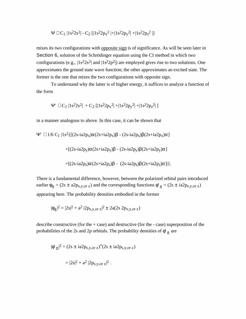
Ψ ≅ C1 |1s22s2| - C2 [|1s22px2 |+|1s22py2| +|1s22pz2 |]
mixes its two configurations with opposite sign is of significance. As will be seen later in
Section 6, solution of the Schrödinger equation using the CI method in which two
configurations (e.g., |1s22s2| and |1s22p2|) are employed gives rise to two solutions. One
approximates the ground state wave function; the other approximates an excited state. The
former is the one that mixes the two configurations with opposite sign.
To understand why the latter is of higher energy, it suffices to analyze a function of
the form
Ψ' ≅ C1 |1s22s2| + C2 [|1s22px2| +|1s22py2| +|1s22pz2| ]
in a manner analogous to above. In this case, it can be shown that
Ψ' ≅ 1/6 C1 |1s2{[(2s-ia2px)α(2s+ia2px)β - (2s-ia2px)β(2s+ia2px)α]
+[(2s-ia2py)α(2s+ia2py)β - (2s-ia2py)β(2s+ia2py)α]
+[(2s-ia2pz)α(2s+ia2pz)β - (2s-ia2pz)β(2s+ia2pz)α]|}.
There is a fundamental difference, however, between the polarized orbital pairs introducedearlier φ± = (2s ± a2px,y,or z) and the corresponding functions φ' ± = (2s ± ia2px,y,or z)
appearing here. The probability densities embodied in the former
|φ±|2 = |2s|2 + a2 |2px,y,or z |2 ± 2a(2s 2px,y,or z)
describe constructive (for the + case) and destructive (for the - case) superposition of theprobabilities of the 2s and 2p orbitals. The probability densities of φ' ± are
|φ' ±|2 = (2s ± ia2px,y,or z)*(2s ± ia2px,y,or z)
= |2s|2 + a2 |2px,y,or z |2 .

These densities are identical to one another and do not describe polarized orbital densities.
Therefore, the CI wavefunction which mixes the two configurations with like sign, whenanalyzed in terms of orbital pairs, places the electrons into orbitals φ' ±=(2s ± ia2px,y,or z)
whose densities do not permit the electrons to avoid one another. Rather, both orbitals have
the same spatial density |2s|2 + a2
|2px,y,or z |2 , which gives rise to higher coulombic interaction energy for this state.
V. Summary
In summary, the dynamical interactions among electrons give rise to instantaneous
spatial correlations that must be handled to arrive at an accurate picture of atomic and
molecular structure. The simple, single-configuration picture provided by the mean-field
model is a useful starting point, but improvements are often needed.
In Section 6, methods for treating electron correlation will be discussed in greater detail.
For the remainder of this Section, the primary focus is placed on forming proper N-
electron wavefunctions by occupying the orbitals available to the system in a manner that
guarantees that the resultant N-electron function is an eigenfunction of those operators that
commute with the N-electron Hamiltonian.
For polyatomic molecules, these operators include point-group symmetry operators
(which act on all N electrons) and the spin angular momentum (S2 and Sz) of all of the
electrons taken as a whole (this is true in the absence of spin-orbit coupling which is treated
later as a perturbation). For linear molecules, the point group symmetry operations involve
rotations Rz of all N electrons about the principal axis, as a result of which the total angular
momentum Lz of the N electrons (taken as a whole) about this axis commutes with the
Hamiltonian, H. Rotation of all N electrons about the x and y axes does not leave the total
coulombic potential energy unchanged, so Lx and Ly do not commute with H. Hence for a
linear molecule, Lz , S2, and Sz are the operators that commute with H. For atoms, the
corresponding operators are L2, Lz, S2, and Sz (again, in the absence of spin-orbit
coupling) where each operator pertains to the total orbital or spin angular momentum of the
N electrons.
To construct N-electron functions that are eigenfunctions of the spatial symmetry or
orbital angular momentum operators as well as the spin angular momentum operators, one
has to "couple" the symmetry or angular momentum properties of the individual spin-
orbitals used to construct the N-electrons functions. This coupling involves forming direct
product symmetries in the case of polyatomic molecules that belong to finite point groups,

it involves vector coupling orbital and spin angular momenta in the case of atoms, and it
involves vector coupling spin angular momenta and axis coupling orbital angular momenta
when treating linear molecules. Much of this Section is devoted to developing the tools
needed to carry out these couplings.
Chapter 9
Electronic Wavefuntions Must be Constructed to Have Permutational Antisymmetry
Because the N Electrons are Indistinguishable Fermions
I. Electronic Configurations
Atoms, linear molecules, and non-linear molecules have orbitals which can be
labeled either according to the symmetry appropriate for that isolated species or for the
species in an environment which produces lower symmetry. These orbitals should be
viewed as regions of space in which electrons can move, with, of course, at most two
electrons (of opposite spin) in each orbital. Specification of a particular occupancy of the
set of orbitals available to the system gives an electronic configuration . For example,
1s22s22p4 is an electronic configuration for the Oxygen atom (and for the F+1 ion and the
N-1 ion); 1s22s22p33p1 is another configuration for O, F+1, or N-1. These configurations
represent situations in which the electrons occupy low-energy orbitals of the system and, as
such, are likely to contribute strongly to the true ground and low-lying excited states and to
the low-energy states of molecules formed from these atoms or ions.
Specification of an electronic configuration does not, however, specify a particular
electronic state of the system. In the above 1s22s22p4 example, there are many ways
(fifteen, to be precise) in which the 2p orbitals can be occupied by the four electrons. As a
result, there are a total of fifteen states which cluster into three energetically distinct levels ,
lying within this single configuration. The 1s22s22p33p1 configuration contains thirty-six
states which group into six distinct energy levels (the word level is used to denote one or
more state with the same energy). Not all states which arise from a given electronic
configuration have the same energy because various states occupy the degenerate (e.g., 2p
and 3p in the above examples) orbitals differently. That is, some states have orbital

occupancies of the form 2p212p102p1-1 while others have 2p212p202p0-1; as a result, the
states can have quite different coulombic repulsions among the electrons (the state with two
doubly occupied orbitals would lie higher in energy than that with two singly occupied
orbitals). Later in this Section and in Appendix G techniques for constructing
wavefunctions for each state contained within a particular configuration are given in detail.
Mastering these tools is an important aspect of learning the material in this text.
In summary, an atom or molecule has many orbitals (core, bonding, non-bonding,
Rydberg, and antibonding) available to it; occupancy of these orbitals in a particular manner
gives rise to a configuration. If some orbitals are partially occupied in this configuration,
more than one state will arise; these states can differ in energy due to differences in how the
orbitals are occupied. In particular, if degenerate orbitals are partially occupied, many states
can arise and have energies which differ substantially because of differences in electron
repulsions arising in these states. Systematic procedures for extracting all states from a
given configuration, for labeling the states according to the appropriate symmetry group,
for writing the wavefunctions corresponding to each state and for evaluating the energies
corresponding to these wavefunctions are needed. Much of Chapters 10 and 11 are
devoted to developing and illustrating these tools.
II. Antisymmetric Wavefunctions
A. General Concepts
The total electronic Hamiltonian
H = Σ i (- h2/2me ∇i2 -Σa Za e2/ria) +Σ i>j e2/rij +Σa>b Za Zbe2/rab,
where i and j label electrons and a and b label the nuclei (whose charges are denoted Za),
commutes with the operators Pij which permute the names of the electrons i and j. This, in
turn, requires eigenfunctions of H to be eigenfunctions of Pij. In fact, the set of such
permutation operators form a group called the symmetric group (a good reference to this
subject is contained in Chapter 7 of Group Theory , M. Hamermesh, Addison-Wesley,
Reading, Mass. (1962)). In the present text, we will not exploit the full group theoretical
nature of these operators; we will focus on the simple fact that all wavefunctions must be
eigenfunctions of the Pij (additional material on this subject is contained in Chapter XIV of
Kemble).

Because Pij obeys Pij * Pij = 1, the eigenvalues of the Pij operators must be +1 or -
1. Electrons are Fermions (i.e., they have half-integral spin), and they have wavefunctions
which are odd under permutation of any pair: Pij Ψ = -Ψ. Bosons such as photons or
deuterium nuclei (i.e., species with integral spin quantum numbers) have wavefunctions
which obey Pij Ψ = +Ψ.These permutational symmetries are not only characteristics of the exact
eigenfunctions of H belonging to any atom or molecule containing more than a single
electron but they are also conditions which must be placed on any acceptable model or trial
wavefunction (e.g., in a variational sense) which one constructs.
In particular, within the orbital model of electronic structure (which is developed
more systematically in Section 6), one can not construct trial wavefunctions which are
simple spin-orbital products (i.e., an orbital multiplied by an α or β spin function for each
electron) such as 1sα1sβ2sα2sβ2p1α2p0α. Such spin-orbital product functions must be
made permutationally antisymmetric if the N-electron trial function is to be properly
antisymmetric. This can be accomplished for any such product wavefunction by applying
the following antisymmetrizer operator :
A = (√1/N!)Σp sp P,
where N is the number of electrons, P runs over all N! permutations, and sp is +1 or -1
depending on whether the permutation P contains an even or odd number of pairwise
permutations (e.g., 231 can be reached from 123 by two pairwise permutations-
123==>213==>231, so 231 would have sp =1). The permutation operator P in A acts on a
product wavefunction and permutes the ordering of the spin-orbitals. For example, A
φ1φ2φ3 = (1/√6) [φ1φ2φ3 -φ1φ3φ2 -φ3φ2φ1 -φ2φ1φ3 +φ3φ1φ2 +φ2φ3φ1], where the
convention is that electronic coordinates r1, r2, and r3 correspond to the orbitals as they
appear in the product (e.g., the term φ3φ2φ1 represents φ3(r1)φ2(r2)φ1(r3)).
It turns out that the permutations P can be allowed either to act on the "names" or
labels of the electrons, keeping the order of the spin-orbitals fixed, or to act on the spin-
orbitals, keeping the order and identity of the electrons' labels fixed. The resultant
wavefunction, which contains N! terms, is exactly the same regardless of how one allows
the permutations to act. Because we wish to use the above convention in which the order of
the electronic labels remains fixed as 1, 2, 3, ... N, we choose to think of the permutations
acting on the names of the spin-orbitals.
It should be noted that the effect of A on any spin-orbital product is to produce a
function that is a sum of N! terms. In each of these terms the same spin-orbitals appear, but
the order in which they appear differs from term to term. Thus antisymmetrization does not
alter the overall orbital occupancy; it simply "scrambles" any knowledge of which electron
is in which spin-orbital.
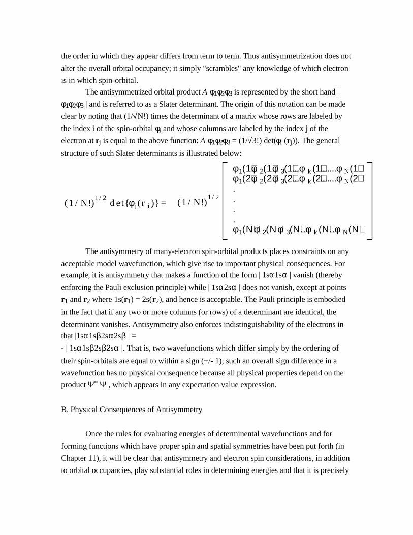
The antisymmetrized orbital product A φ1φ2φ3 is represented by the short hand |
φ1φ2φ3 | and is referred to as a Slater determinant . The origin of this notation can be made
clear by noting that (1/√N!) times the determinant of a matrix whose rows are labeled by
the index i of the spin-orbital φi and whose columns are labeled by the index j of the
electron at rj is equal to the above function: A φ1φ2φ3 = (1/√3!) det(φi (rj)). The general
structure of such Slater determinants is illustrated below:
(1/N!)1/2
det{φ j(r i)} = (1/N!)1/2
φ 1(1)φ2(1)φ3(1)...φk(1).......φN(1)φ 1(2)φ2(2)φ3(2)...φk(2).......φN(2)....φ 1(Ν)φ2(Ν)φ3(Ν)..φk(Ν)..φN(Ν)
The antisymmetry of many-electron spin-orbital products places constraints on any
acceptable model wavefunction, which give rise to important physical consequences. For
example, it is antisymmetry that makes a function of the form | 1sα1sα | vanish (thereby
enforcing the Pauli exclusion principle) while | 1sα2sα | does not vanish, except at points
r1 and r2 where 1s(r1) = 2s(r2), and hence is acceptable. The Pauli principle is embodied
in the fact that if any two or more columns (or rows) of a determinant are identical, the
determinant vanishes. Antisymmetry also enforces indistinguishability of the electrons in
that |1sα1sβ2sα2sβ | =
- | 1sα1sβ2sβ2sα |. That is, two wavefunctions which differ simply by the ordering of
their spin-orbitals are equal to within a sign (+/- 1); such an overall sign difference in a
wavefunction has no physical consequence because all physical properties depend on the
product Ψ* Ψ , which appears in any expectation value expression.
B. Physical Consequences of Antisymmetry
Once the rules for evaluating energies of determinental wavefunctions and for
forming functions which have proper spin and spatial symmetries have been put forth (in
Chapter 11), it will be clear that antisymmetry and electron spin considerations, in addition
to orbital occupancies, play substantial roles in determining energies and that it is precisely

these aspects that are responsible for energy splittings among states arising from one
configuration. A single example may help illustrate this point. Consider the π1π*1
configuration of ethylene (ignore the other orbitals and focus on the properties of these
two). As will be shown below when spin angular momentum is treated in full, the triplet
spin states of this configuration are:
|S=1, MS=1> = |παπ*α|,
|S=1, MS=-1> = |πβπ*β|,
and
|S=1, MS= 0> = 2-1/2[ |παπ*β| + |πβπ*α|].
The singlet spin state is:
|S=0, MS= 0> = 2-1/2[ |παπ*β| - |πβπ*α|].
To understand how the three triplet states have the same energy and why the singlet
state has a different energy, and an energy different than the MS= 0 triplet even though
these two states are composed of the same two determinants, we proceed as follows:
1. We express the bonding π and antibonding π* orbitals in terms of the atomic p-orbitals
from which they are formed: π= 2-1/2 [ L + R ] and π* = 2-1/2 [ L - R ], where R and L
denote the p-orbitals on the left and right carbon atoms, respectively.
2. We substitute these expressions into the Slater determinants that form the singlet and
triplet states and collect terms and throw out terms for which the determinants vanish.
3. This then gives the singlet and triplet states in terms of atomic-orbital occupancies where
it is easier to see the energy equivalences and differences.
Let us begin with the triplet states:
|παπ*α| = 1/2 [ |LαLα| - |RαRα| + |RαLα| - |LαRα| ]
= |RαLα|;

2-1/2[ |παπ*β| + |πβπ*α|] = 2-1/2 1/2[ |LαLβ| - |RαRβ| + |RαLβ| -
|LαRβ| + |LβLα| - |RβRα| + |RβLα| - |LβRα| ]
= 2-1/2 [ |RαLβ| + |RβLα| ];
|πβπ*β| = 1/2 [ |LβLβ| - |RβRβ| + |RβLβ| - |LβRβ| ]
= |RβLβ|.
The singlet state can be reduced in like fashion:
2-1/2[ |παπ*β| - |πβπ*α|] = 2-1/2 1/2[ |LαLβ| - |RαRβ| + |RαLβ| -
|LαRβ| - |LβLα| + |RβRα| - |RβLα| + |LβRα| ]
= 2-1/2 [ |LαLβ| - |RβRα| ].
Notice that all three triplet states involve atomic orbital occupancy in which one electron is
on one atom while the other is on the second carbon atom. In contrast, the singlet state
places both electrons on one carbon (it contains two terms; one with the two electrons on
the left carbon and the other with both electrons on the right carbon).
In a "valence bond" analysis of the physical content of the singlet and triplet π1π*1
states, it is clear that the energy of the triplet states will lie below that of the singlet because
the singlet contains "zwitterion" components that can be denoted C+C- and C-C+, while the
three triplet states are purely "covalent". This case provides an excellent example of how
the spin and permutational symmetries of a state "conspire" to qualitatively affect its energy
and even electronic character as represented in its atomic orbital occupancies.
Understanding this should provide ample motivation for learning how to form proper
antisymmetric spin (and orbital) angular momentum eigenfunctions for atoms and
molecules.

Chapter 10
Electronic Wavefunctions Must Also Possess Proper Symmetry. These Include Angular
Momentum and Point Group Symmetries
I. Angular Momentum Symmetry and Strategies for Angular Momentum Coupling
Because the total Hamiltonian of a many-electron atom or molecule forms a
mutually commutative set of operators with S2 , Sz , and A = (√1/N!)Σp sp P, the exact
eigenfunctions of H must be eigenfunctions of these operators. Being an eigenfunction of
A forces the eigenstates to be odd under all Pij. Any acceptable model or trial wavefunction
should be constrained to also be an eigenfunction of these symmetry operators.
If the atom or molecule has additional symmetries (e.g., full rotation symmetry for
atoms, axial rotation symmetry for linear molecules and point group symmetry for non-
linear polyatomics), the trial wavefunctions should also conform to these spatial
symmetries. This Chapter addresses those operators that commute with H, Pij, S2, and Sz
and among one another for atoms, linear, and non-linear molecules.
As treated in detail in Appendix G, the full non-relativistic N-electron Hamiltonian
of an atom or molecule
H = Σ j(- h2/2m ∇j2 - Σa Zae2/rj,a) + Σ j<k e2/rj,k
commutes with the following operators:
i. The inversion operator i and the three components of the total orbital angular momentum
Lz = Σ jLz(j), Ly, Lx, as well as the components of the total spin angular momentum Sz, Sx,
and Sy for atoms (but not the individual electrons' Lz(j) , Sz(j), etc). Hence, L2, Lz, S2,
Sz are the operators we need to form eigenfunctions of, and L, ML, S, and MS are the
"good" quantum numbers.
ii. Lz = Σ jLz(j), as well as the N-electron Sx, Sy, and Sz for linear molecules (also i, if
the molecule has a center of symmetry). Hence, Lz, S2, and Sz are the operators we need to

form eigenfunctions of, and ML, S, and MS are the "good" quantum numbers; L no longer
is!
iii. Sx, Sy, and Sz as well as all point group operations for non-linear polyatomic
molecules. Hence S2, Sz, and the point group operations are used to characterize the
functions we need to form. When we include spin-orbit coupling into H (this adds another
term to the potential that involves the spin and orbital angular momenta of the electrons),
L2, Lz, S2, Sz no longer commute with H. However, Jz = Sz + Lz and J2 = (L+S )2 now
do commute with H.
A. Electron Spin Angular Momentum
Individual electrons possess intrinsic spin characterized by angular momentum
quantum numbers s and ms ; for electrons, s = 1/2 and ms = 1/2, or -1/2. The ms =1/2 spin
state of the electron is represented by the symbol α and the ms = -1/2 state is represented by
β. These spin functions obey: S2 α = 1/2 (1/2 + 1)h2 α,Sz α = 1/2h α, S2 β =1/2 (1/2 + 1) h2β, and Sz β = -1/2hβ. The α and β spin functions
are connected via lowering S- and raising S+ operators, which are defined in terms of the x
and y components of S as follows: S+ = Sx +iSy, and S - = Sx -iSy. In particular S+β =
hα, S+α =0, S-α = hβ,and S-β =0. These expressions are examples of the more general relations (these relations
are developed in detail in Appendix G) which all angular momentum operators and their
eigenstates obey:
J2 |j,m> = j(j+1)h2 |j,m>,
Jz |j,m> = mh |j,m>,
J+ |j,m> =h {j(j+1)-m(m+1)}1/2 |j,m+1>, and
J- |j,m> =h {j(j+1)-m(m-1)}1/2 |j,m-1>.
In a many-electron system, one must combine the spin functions of the individual
electrons to generate eigenfunctions of the total Sz =Σ i Sz(i) ( expressions for Sx =Σ i Sx(i)
and Sy =Σ i Sy(i) also follow from the fact that the total angular momentum of a collection
of particles is the sum of the angular momenta, component-by-component, of the individual

angular momenta) and total S2 operators because only these operators commute with the
full Hamiltonian, H, and with the permutation operators Pij. No longer are the individual
S2(i) and Sz(i) good quantum numbers; these operators do not commute with Pij.
Spin states which are eigenfunctions of the total S2 and Sz can be formed by using
angular momentum coupling methods or the explicit construction methods detailed in
Appendix (G). In the latter approach, one forms, consistent with the given electronic
configuration, the spin state having maximum Sz eigenvalue (which is easy to identify as
shown below and which corresponds to a state with S equal to this maximum Sz
eigenvalue) and then generating states of lower Sz values and lower S values using the
angular momentum raising and lowering operators (S- =Σ i S- (i) and
S+ =Σ i S+ (i)).
To illustrate, consider a three-electron example with the configuration 1s2s3s.
Starting with the determinant | 1sα2sα3sα |, which has the maximum Ms =3/2 and hence
has S=3/2 (this function is denoted |3/2, 3/2>), apply S- in the additive form S- =Σ i S-(i) to
generate the following combination of three determinants:
h[| 1sβ2sα3sα | + | 1sα2sβ3sα | + | 1sα2sα3sβ |],
which, according to the above identities, must equal
h 3/2(3/2+1)-3/2(3/2-1) | 3/2, 1/2>.
So the state |3/2, 1/2> with S=3/2 and Ms =1/2 can be solved for in terms of the three
determinants to give
|3/2, 1/2> = 1/√3[ | 1sβ2sα3sα | + | 1sα2sβ3sα | + | 1sα2sα3sβ | ].
The states with S=3/2 and Ms = -1/2 and -3/2 can be obtained by further application of S- to
|3/2, 1/2> (actually, the Ms= -3/2 can be identified as the "spin flipped" image of the state
with Ms =3/2 and the one with Ms =-1/2 can be formed by interchanging all α's and β's in
the Ms = 1/2 state).
Of the eight total spin states (each electron can take on either α or β spin and there
are three electrons, so the number of states is 23), the above process has identified proper
combinations which yield the four states with S= 3/2. Doing so consumed the determinants
with Ms =3/2 and -3/2, one combination of the three determinants with MS =1/2, and one
combination of the three determinants with Ms =-1/2. There still remain two combinations

of the Ms =1/2 and two combinations of the Ms =-1/2 determinants to deal with. These
functions correspond to two sets of S = 1/2 eigenfunctions having
Ms = 1/2 and -1/2. Combinations of the determinants must be used in forming the S = 1/2
functions to keep the S = 1/2 eigenfunctions orthogonal to the above S = 3/2 functions
(which is required because S2 is a hermitian operator whose eigenfunctions belonging to
different eigenvalues must be orthogonal). The two independent S = 1/2, Ms = 1/2 states
can be formed by simply constructing combinations of the above three determinants with
Ms =1/2 which are orthogonal to the S = 3/2 combination given above and orthogonal to
each other. For example,
| 1/2, 1/2> = 1/√2[ | 1sβ2sα3sα | - | 1sα2sβ3sα | + 0x | 1sα2sα3sβ | ],
| 1/2, 1/2> = 1/√6[ | 1sβ2sα3sα | + | 1sα2sβ3sα | -2x | 1sα2sα3sβ | ]
are acceptable (as is any combination of these two functions generated by a unitary
transformation ). A pair of independent orthonormal states with S =1/2 and Ms = -1/2 can
be generated by applying S- to each of these two functions ( or by constructing a pair of
orthonormal functions which are combinations of the three determinants with Ms = -1/2 and
which are orthogonal to the S=3/2, Ms = -1/2 function obtained as detailed above).
The above treatment of a three-electron case shows how to generate quartet (spin
states are named in terms of their spin degeneracies 2S+1) and doublet states for a
configuration of the form
1s2s3s. Not all three-electron configurations have both quartet and doublet states; for
example, the 1s2 2s configuration only supports one doublet state. The methods used
above to generate S = 3/2 and
S = 1/2 states are valid for any three-electron situation; however, some of the determinental
functions vanish if doubly occupied orbitals occur as for 1s22s. In particular, the |
1sα1sα2sα | and
| 1sβ1sβ2sβ | Ms =3/2, -3/2 and | 1sα1sα2sβ | and | 1sβ1sβ2sα | Ms = 1/2, -1/2
determinants vanish because they violate the Pauli principle; only | 1sα1sβ2sα | and |
1sα1sβ2sβ | do not vanish. These two remaining determinants form the S = 1/2, Ms = 1/2,
-1/2 doublet spin functions which pertain to the 1s22s configuration. It should be noted that
all closed-shell components of a configuration (e.g., the 1s2 part of 1s22s or the 1s22s2 2p6
part of 1s22s2 2p63s13p1 ) must involve α and β spin functions for each doubly occupied
orbital and, as such, can contribute nothing to the total Ms value; only the open-shell

components need to be treated with the angular momentum operator tools to arrive at proper
total-spin eigenstates.
In summary, proper spin eigenfunctions must be constructed from antisymmetric
(i.e., determinental) wavefunctions as demonstrated above because the total S2 and total Sz
remain valid symmetry operators for many-electron systems. Doing so results in the spin-
adapted wavefunctions being expressed as combinations of determinants with coefficients
determined via spin angular momentum techniques as demonstrated above. In
configurations with closed-shell components, not all spin functions are possible because of
the antisymmetry of the wavefunction; in particular, any closed-shell parts must involve αβspin pairings for each of the doubly occupied orbitals, and, as such, contribute zero to the
total Ms.
B. Vector Coupling of Angular Momenta
Given two angular momenta (of any kind) L1 and L2, when one generates states
that are eigenstates of their vector sum L= L1+L2,
one can obtain L values of L1+L2, L1+L2-1, ...|L1-L2|. This can apply to two electrons for
which the total spin S can be 1 or 0 as illustrated in detail above, or to a p and a d orbital for
which the total orbital angular momentum L can be 3, 2, or 1. Thus for a p1d1 electronic
configuration, 3F, 1F, 3D, 1D, 3P, and 1P energy levels (and corresponding
wavefunctions) arise. Here the term symbols are specified as the spin degeneracy (2S+1)
and the letter that is associated with the L-value. If spin-orbit coupling is present, the 3F
level further splits into J= 4, 3, and 2 levels which are denoted 3F4, 3F3, and 3F2.
This simple "vector coupling" method applies to any angular momenta. However, if
the angular momenta are "equivalent" in the sense that they involve indistinguishable
particles that occupy the same orbital shell (e.g., 2p3 involves 3 equivalent electrons;
2p13p14p1 involves 3 non-equivalent electrons; 2p23p1 involves 2 equivalent electrons and
one non-equivalent electron), the Pauli principle eliminates some of the expected term
symbols (i.e., when the corresponding wavefunctions are formed, some vanish because
their Slater determinants vanish). Later in this section, techniques for dealing with the
equivalent-angular momenta case are introduced. These techniques involve using the above
tools to obtain a list of candidate term symbols after which Pauli-violating term symbols are
eliminated.
C. Non-Vector Coupling of Angular Momenta

For linear molecules, one does not vector couple the orbital angular momenta of the
individual electrons (because only Lz not L2 commutes with H), but one does vector couple
the electrons' spin angular momenta. Coupling of the electrons' orbital angular momenta
involves simply considering the various Lz eigenvalues that can arise from adding the Lz
values of the individual electrons. For example, coupling two π orbitals (each of which can
have m = ±1) can give ML=1+1, 1-1, -1+1, and -1-1, or 2, 0, 0, and -2. The level with
ML = ±2 is called a ∆ state (much like an orbital with m = ±2 is called a δ orbital), and the
two states with ML = 0 are called Σ states. States with Lz eigenvalues of ML and - ML are
degenerate because the total energy is independent of which direction the electrons are
moving about the linear molecule's axis (just a π+1 and π-1 orbitals are degenerate).
Again, if the two electrons are non-equivalent, all possible couplings arise (e.g., a
π1π' 1 configuration yields 3∆, 3Σ, 3Σ, 1∆, 1Σ, and 1Σ states). In contrast, if the two
electrons are equivalent, certain of the term symbols are Pauli forbidden. Again, techniques
for dealing with such cases are treated later in this Chapter.
D. Direct Products for Non-Linear Molecules
For non-linear polyatomic molecules, one vector couples the electrons' spin angular
momenta but their orbital angular momenta are not even considered. Instead, their point
group symmetries must be combined, by forming direct products, to determine the
symmetries of the resultant spin-orbital product states. For example, the b11b21
configuration in C2v symmetry gives rise to 3A2 and 1A2 term symbols. The e1e'1
configuration in C3v symmetry gives 3E, 3A2, 3A1, 1E, 1A2, and 1A1 term symbols. For
two equivalent electrons such as in the e2 configuration, certain of the 3E, 3A2, 3A1, 1E,1A2, and 1A1 term symbols are Pauli forbidden. Once again, the methods needed to
identify which term symbols arise in the equivalent-electron case are treated later.
One needs to learn how to tell which term symbols will be Pauli excluded, and to
learn how to write the spin-orbit product wavefunctions corresponding to each term symbol
and to evaluate the corresponding term symbols' energies.
II. Atomic Term Symbols and Wavefunctions
A. Non-Equivalent Orbital Term Symbols
When coupling non-equivalent angular momenta (e.g., a spin and an orbital angular
momenta or two orbital angular momenta of non-equivalent electrons), one vector couples

using the fact that the coupled angular momenta range from the sum of the two individual
angular momenta to the absolute value of their difference. For example, when coupling the
spins of two electrons, the total spin S can be 1 or 0; when coupling a p and a d orbital, the
total orbital angular momentum can be 3, 2, or 1. Thus for a p1d1 electronic configuration,3F, 1F, 3D, 1D, 3P, and 1P energy levels (and corresponding wavefunctions) arise. The
energy differences among these levels has to do with the different electron-electron
repulsions that occur in these levels; that is, their wavefunctions involve different
occupancy of the p and d orbitals and hence different repulsion energies. If spin-orbit
coupling is present, the L and S angular momenta are further vector coupled. For example,
the 3F level splits into J= 4, 3, and 2 levels which are denoted 3F4, 3F3, and 3F2. The
energy differences among these J-levels are caused by spin-orbit interactions.
B. Equivalent Orbital Term Symbols
If equivalent angular momenta are coupled (e.g., to couple the orbital angular
momenta of a p2 or d3 configuration), one must use the "box" method to determine which
of the term symbols, that would be expected to arise if the angular momenta were non-
equivalent, violate the Pauli principle. To carry out this step, one forms all possible unique
(determinental) product states with non-negative ML and MS values and arranges them into
groups according to their ML and MS values. For example, the boxes appropriate to the p2
orbital occupancy are shown below:

ML 2 1 0
---------------------------------------------------------
MS 1 |p1αp0α| |p1αp-1α|
0 |p1αp1β| |p1αp0β|, |p0αp1β| |p1αp-1β|,
|p-1αp1β|,
|p0αp0β|
There is no need to form the corresponding states with negative ML or negative MS values
because they are simply "mirror images" of those listed above. For example, the state with
ML= -1 and MS = -1 is |p-1βp0β|, which can be obtained from the ML = 1, MS = 1 state
|p1αp0α| by replacing α by β and replacing p1 by p-1.
Given the box entries, one can identify those term symbols that arise by applying
the following procedure over and over until all entries have been accounted for:
1. One identifies the highest MS value (this gives a value of the total spin quantum number
that arises, S) in the box. For the above example, the answer is S = 1.
2. For all product states of this MS value, one identifies the highest ML value (this gives a
value of the total orbital angular momentum, L, that can arise for this S ). For the above
example, the highest ML within the MS =1 states is ML = 1 (not ML = 2), hence L=1.
3. Knowing an S, L combination, one knows the first term symbol that arises from this
configuration. In the p2 example, this is 3P.
4. Because the level with this L and S quantum numbers contains (2L+1)(2S+1) states with
ML and MS quantum numbers running from -L to L and from -S to S, respectively, one
must remove from the original box this number of product states. To do so, one simply
erases from the box one entry with each such ML and MS value. Actually, since the box
need only show those entries with non-negative ML and MS values, only these entries need
be explicitly deleted. In the 3P example, this amounts to deleting nine product states with
ML, MS values of 1,1; 1,0; 1,-1; 0,1; 0,0; 0,-1; -1,1; -1,0; -1,-1.
5. After deleting these entries, one returns to step 1 and carries out the process again. For
the p2 example, the box after deleting the first nine product states looks as follows (those
that appear in italics should be viewed as already cancelled in counting all of the 3P states):
ML 2 1 0
---------------------------------------------------------

MS 1 |p1αp0α| |p1αp-1α|
0 |p1αp1β| |p1αp0β|, |p0αp1β| |p1αp-1β|,
|p-1αp1β|,
|p0αp0β|
It should be emphasized that the process of deleting or crossing off entries in various ML,
MS boxes involves only counting how many states there are; by no means do we identify
the particular L,S,ML,MS wavefunctions when we cross out any particular entry in a box.
For example, when the |p1αp0β| product is deleted from the ML= 1, MS=0 box in
accounting for the states in the 3P level, we do not claim that |p1αp0β| itself is a member of
the 3P level; the |p0αp1β| product state could just as well been eliminated when accounting
for the 3P states. As will be shown later, the 3P state with ML= 1, MS=0 will be a
combination of |p1αp0β| and |p0αp1β|.
Returning to the p2 example at hand, after the 3P term symbol's states have been
accounted for, the highest MS value is 0 (hence there is an S=0 state), and within this MS
value, the highest ML value is 2 (hence there is an L=2 state). This means there is a 1D
level with five states having ML = 2,1,0,-1,-2. Deleting five appropriate entries from the
above box (again denoting deletions by italics) leaves the following box:

ML 2 1 0
---------------------------------------------------------
MS 1 |p1αp0α| |p1αp-1α|
0 |p1αp1β| |p1αp0β|, |p0αp1β| |p1αp-1β|,
|p-1αp1β|,
|p0αp0β|
The only remaining entry, which thus has the highest MS and ML values, has MS = 0 and
ML = 0. Thus there is also a 1S level in the p2 configuration.
Thus, unlike the non-equivalent 2p13p1 case, in which 3P, 1P, 3D, 1D, 3S, and 1S
levels arise, only the 3P, 1D, and 1S arise in the p2 situation. This "box method" is
necessary to carry out whenever one is dealing with equivalent angular momenta.
If one has mixed equivalent and non-equivalent angular momenta, one can
determine all possible couplings of the equivalent angular momenta using this method and
then use the simpler vector coupling method to add the non-equivalent angular momenta to
each of these coupled angular momenta. For example, the p2d1 configuration can be
handled by vector coupling (using the straightforward non-equivalent procedure) L=2 (the
d orbital) and S=1/2 (the third electron's spin) to each of 3P, 1D, and 1S. The result is 4F,4D, 4P, 2F, 2D, 2P, 2G, 2F, 2D, 2P, 2S, and 2D.
C. Atomic Configuration Wavefunctions
To express, in terms of Slater determinants, the wavefunctions corresponding to
each of the states in each of the levels, one proceeds as follows:
1. For each MS, ML combination for which one can write down only one product function
(i.e., in the non-equivalent angular momentum situation, for each case where only one
product function sits at a given box row and column point), that product function itself is
one of the desired states. For the p2 example, the |p1αp0α| and |p1αp-1α| (as well as their
four other ML and MS "mirror images") are members of the 3P level (since they have MS =
±1) and |p1αp1β| and its ML mirror image are members of the 1D level (since they have ML
= ±2).

2. After identifying as many such states as possible by inspection, one uses L± and S± to
generate states that belong to the same term symbols as those already identified but which
have higher or lower ML and/or MS values.
3. If, after applying the above process, there are term symbols for which states have not yet
been formed, one may have to construct such states by forming linear combinations that are
orthogonal to all those states that have thus far been found.
To illustrate the use of raising and lowering operators to find the states that can not
be identified by inspection, let us again focus on the p2 case. Beginning with three of the3P states that are easy to recognize, |p1αp0α|, |p1αp-1α|, and |p-1αp0α|, we apply S- to
obtain the MS=0 functions:
S- 3P(ML=1, MS=1) = [S-(1) + S-(2)] |p1αp0α|
= h(1(2)-1(0))1/2 3P(ML=1, MS=0)
= h(1/2(3/2)-1/2(-1/2))1/2 |p1βp0α| + h(1)1/2 |p1αp0β|,
so,3P(ML=1, MS=0) = 2-1/2 [|p1βp0α| + |p1αp0β|].
The same process applied to |p1αp-1α| and |p-1αp0α| gives
1/√2[||p1αp-1β| + |p1βp-1α|] and 1/√2[||p-1αp0β| + |p-1βp0α|],
respectively.
The 3P(ML=1, MS=0) = 2-1/2 [|p1βp0α| + |p1αp0β| function can be acted on with
L- to generate 3P(ML=0, MS=0):
L- 3P(ML=1, MS=0) = [L-(1) + L-(2)] 2-1/2 [|p1βp0α| + |p1αp0β|]
= h(1(2)-1(0))1/2 3P(ML=0, MS=0)
=h(1(2)-1(0))1/2 2-1/2 [|p0βp0α| + |p0αp0β|]
+ h (1(2)-0(-1))1/2 2-1/2 [|p1βp-1α| + |p1αp-1β|],
so,3P(ML=0, MS=0) = 2-1/2 [|p1βp-1α| + |p1αp-1β|].

The 1D term symbol is handled in like fashion. Beginning with the ML = 2 state
|p1αp1β|, one applies L- to generate the ML = 1 state:
L- 1D(ML=2, MS=0) = [L-(1) + L-(2)] |p1αp1β|
= h(2(3)-2(1))1/2 1D(ML=1, MS=0)
= h(1(2)-1(0))1/2 [|p0αp1β| + |p1αp0β|],
so,1D(ML=1, MS=0) = 2-1/2 [|p0αp1β| + |p1αp0β|].
Applying L- once more generates the 1D(ML=0, MS=0) state:
L- 1D(ML=1, MS=0) = [L-(1) + L-(2)] 2-1/2 [|p0αp1β| + |p1αp0β|]
= h(2(3)-1(0))1/2 1D(ML=0, MS=0)
= h(1(2)-0(-1))1/2 2-1/2 [|p-1αp1β| + |p1αp-1β|]
+ h(1(2)-1(0))1/2 2-1/2 [|p0αp0β| + |p0αp0β|],
so,1D(ML=0, MS=0) = 6-1/2[ 2|p0αp0β| + |p-1αp1β| + |p1αp-1β|].
Notice that the ML=0, MS=0 states of 3P and of 1D are given in terms of the three
determinants that appear in the "center" of the p2 box diagram:
1D(ML=0, MS=0) = 6-1/2[ 2|p0αp0β| + |p-1αp1β| + |p1αp-1β|],
3P(ML=0, MS=0) = 2-1/2 [|p1βp-1α| + |p1αp-1β|]
= 2-1/2 [ -|p-1αp1β| + |p1αp-1β|].
The only state that has eluded us thus far is the 1S state, which also has ML=0 and MS=0.
To construct this state, which must also be some combination of the three determinants
with ML=0 and MS=0, we use the fact that the 1S wavefunction must be orthogonal to the

3P and 1D functions because 1S, 3P, and 1D are eigenfunctions of the hermitian operator L2
having different eigenvalues. The state that is normalized and is a combination of p0αp0β|,
|p-1αp1β|, and |p1αp-1β| is given as follows:
1S = 3-1/2 [ |p0αp0β| - |p-1αp1β| - |p1αp-1β|].
The procedure used here to form the 1S state illustrates point 3 in the above prescription for
determining wavefunctions. Additional examples for constructing wavefunctions for atoms
are provided later in this chapter and in Appendix G.
D. Inversion Symmetry
One more quantum number, that relating to the inversion (i) symmetry operator can
be used in atomic cases because the total potential energy V is unchanged when all of the
electrons have their position vectors subjected to inversion (i r = -r). This quantum number
is straightforward to determine. Because each L, S, ML, MS, H state discussed above
consist of a few (or, in the case of configuration interaction several) symmetry adapted
combinations of Slater determinant functions, the effect of the inversion operator on such a
wavefunction Ψ can be determined by:
(i) applying i to each orbital occupied in Ψ thereby generating a ± 1 factor for each
orbital (+1 for s, d, g, i, etc orbitals; -1 for p, f, h, j, etc orbitals),
(ii) multiplying these ± 1 factors to produce an overall sign for the character of Ψunder i.
When this overall sign is positive, the function Ψ is termed "even" and its term symbol is
appended with an "e" superscript (e.g., the 3P level of the O atom, which has
1s22s22p4 occupancy is labeled 3Pe); if the sign is negative Ψ is called "odd" and the term
symbol is so amended (e.g., the 3P level of 1s22s12p1 B+ ion is labeled 3Po).
E. Review of Atomic Cases
The orbitals of an atom are labeled by l and m quantum numbers; the orbitals
belonging to a given energy and l value are 2l+1- fold degenerate. The many-electron
Hamiltonian, H, of an atom and the antisymmetrizer operator A = (√1/N!)Σp sp P
commute with total Lz =Σ i Lz (i) , as in the linear-molecule case. The additional symmetry
present in the spherical atom reflects itself in the fact that Lx, and Ly now also commute
with H and A . However, since Lz does not commute with Lx or Ly, new quantum

numbers can not be introduced as symmetry labels for these other components of L. A new
symmetry label does arise when L2 = Lz2 + Lx2 + Ly2 is introduced; L2 commutes with H,
A , and Lz, so proper eigenstates (and trial wavefunctions) can be labeled with L, ML, S,
Ms, and H quantum numbers.
To identify the states which arise from a given atomic configuration and to construct
properly symmetry-adapted determinental wave functions corresponding to these
symmetries, one must employ L and ML and S and MS angular momentum tools. One first
identifies those determinants with maximum MS (this then defines the maximum S value
that occurs); within that set of determinants, one then identifies the determinant(s) with
maximum ML (this identifies the highest L value). This determinant has S and L equal to its
Ms and ML values (this can be verified, for example for L, by acting on this determinant
with L2 in the form
L2 = L-L+ + Lz2 + hLz
and realizing that L+ acting on the state must vanish); other members of this L,S energy
level can be constructed by sequential application of S- and L- = Σ i L-(i) . Having
exhausted a set of (2L+1)(2S+1) combinations of the determinants belonging to the given
configuration, one proceeds to apply the same procedure to the remaining determinants (or
combinations thereof). One identifies the maximum Ms and, within it, the maximum
ML which thereby specifies another S, L label and a new "maximum" state. The
determinental functions corresponding to these L,S (and various ML, Ms ) values can be
constructed by applying S- and L- to this "maximum" state. This process is continued until
all of the states and their determinental wave functions are obtained.
As illustrated above, any p2 configuration gives rise to 3Pe, 1De, and 1Se levels
which contain nine, five, and one state respectively. The use of L and S angular momentum
algebra tools allows one to identify the wavefunctions corresponding to these states. As
shown in detail in Appendix G, in the event that spin-orbit coupling causes the
Hamiltonian, H, not to commute with L or with S but only with their vector sum J= L +S , then these L2 S2 Lz Sz eigenfunctions must be coupled (i.e., recombined) to generate J2
Jz eigenstates. The steps needed to effect this coupling are developed and illustrated for the
above p2 configuration case in Appendix G.
In the case of a pair of non-equivalent p orbitals (e.g., in a 2p13p1 configuration),
even more states would arise. They can also be found using the tools provided above.
Their symmetry labels can be obtained by vector coupling (see Appendix G) the spin and
orbital angular momenta of the two subsystems. The orbital angular momentum coupling

with l = 1 and l = 1 gives L = 2, 1, and 0 or D, P, and S states. The spin angular
momentum coupling with s =1/2 and s = 1/2 gives S = 1 and 0, or triplet and singlet states.
So, vector coupling leads to the prediction that 3De, 1De, 3Pe, 1Pe, 3Se, and 1Se states can
be formed from a pair of non-equivalent p orbitals. It is seen that more states arise when
non-equivalent orbitals are involved; for equivalent orbitals, some determinants vanish,
thereby decreasing the total number of states that arise.
III. Linear Molecule Term Symbols and Wavefunctions
A. Non-Equivalent Orbital Term Symbols
Equivalent angular momenta arising in linear molecules also require use of
specialized angular momentum coupling. Their spin angular momenta are coupled exactly
as in the atomic case because both for atoms and linear molecules, S2 and Sz commute with
H. However, unlike atoms, linear molecules no longer permit L2 to be used as an operator
that commutes with H; Lz still does, but L2 does not. As a result, when coupling non-
equivalent linear molecule angular momenta, one vector couples the electron spins as
before. However, in place of vector coupling the individual orbital angular momenta, one
adds the individual Lz values to obtain the Lz values of the coupled system. For example,
the π1π' 1 configuration gives rise to S=1 and S=0 spin states. The individual ml values of
the two pi-orbitals can be added to give ML = 1+1, 1-1, -1+1, and -1-1, or 2, 0, 0, and -2.
The ML = 2 and -2 cases are degenerate (just as the ml= 2 and -2 δ orbitals are and the ml=
1 and -1 π orbitals are) and are denoted by the term symbol ∆; there are two distinct ML = 0
states that are denoted Σ. Hence, the π1π' 1 configuration yields 3∆, 3Σ, 3Σ, 1∆, 1Σ, and1Σ term symbols.
B. Equivalent-Orbital Term Symbols
To treat the equivalent-orbital case π2, one forms a box diagram as in the atom case:
ML 2 1 0
---------------------------------------------------------
MS 1 |π1απ-1α|
0 |π1απ1β| |π1απ-1β|,

|π-1απ1β|
The process is very similar to that used for atoms. One first identifies the highest
MS value (and hence an S value that occurs) and within that MS , the highest ML.
However, the highest ML does not specify an L-value, because L is no longer a "good
quantum number" because L2 no longer commutes with H. Instead, we simply take the
highest ML value (and minus this value) as specifying a Σ, Π, ∆, Φ, Γ, etc. term symbol.
In the above example, the highest MS value is MS = 1, so there is an S = 1 level. Within
MS = 1, the highest ML = 0; hence, there is a 3Σ level.
After deleting from the box diagram entries corresponding to MS values ranging
from -S to S and ML values of ML and - ML, one has (again using italics to denote the
deleted entries):
ML 2 1 0
---------------------------------------------------------
MS 1 |π1απ-1α|
0 |π1απ1β| |π1απ-1β|,
|π-1απ1β|
Among the remaining entries, the highest MS value is MS = 0, and within this MS the
highest ML is ML = 2. Thus, there is a 1∆ state. Deleting entries with MS = 0 and ML = 2
and -2, one has left the following box diagram:
ML 2 1 0
---------------------------------------------------------
MS 1 |π1απ-1α|
0 |π1απ1β| |π1απ-1β|,
|π-1απ1β|
There still remains an entry with MS = 0 and ML = 0; hence, there is also a 1Σ level.
Recall that the non-equivalent π1π' 1 case yielded 3∆, 3Σ, 3Σ, 1∆, 1Σ, and 1Σ term
symbols. The equivalent π2 case yields only 3Σ, 1∆, and 1Σ term symbols. Again,

whenever one is faced with equivalent angular momenta in a linear-molecule case, one must
use the box method to determine the allowed term symbols. If one has a mixture of
equivalent and non-equivalent angular momenta, it is possible to treat the equivalent angular
momenta using boxes and to then add in the non-equivalent angular momenta using the
more straightforward technique. For example, the π2δ1 configuration can be treated by
coupling the π2 as above to generate 3Σ, 1∆, and 1Σ and then vector coupling the spin of
the third electron and additively coupling the ml = 2 and -2 of the third orbital. The
resulting term symbols are 4∆, 2∆, 2Γ, 2Σ, 2Σ, and 2∆ (e.g., for the 1∆ intermediate state,
adding the δ orbital's ml values gives total ML values of ML = 2+2, 2-2, -2+2, and
-2-2, or 4, 0, 0, and -4).
C. Linear-Molecule Configuration Wavefunctions
Procedures analogous to those used for atoms can be applied to linear molecules.
However, in this case only S± can be used; L± no longer applies because L is no longer a
good quantum number. One begins as in the atom case by identifying determinental
functions for which ML and MS are unique. In the π2 example considered above, these
states include |π1απ-1α|, |π1απ1β|, and their mirror images. These states are members of
the 3Σ and 1∆ levels, respectively, because the first has MS=1 and because the latter has
ML = 2.
Applying S- to this 3Σ state with MS=1 produces the 3Σ state with MS = 0:
S- 3Σ(ML=0, MS=1) = [S-(1) + S-(2)] |π1απ-1α|
= h(1(2)-1(0))1/2 3Σ(ML=0, MS=0)
= h (1)1/2 [|π1βπ-1α| + |π1απ-1β|],
so,3Σ(ML=0, MS=0) = 2-1/2 [|π1βπ-1α| + |π1απ-1β|].
The only other state that can have ML=0 and MS=0 is the 1Σ state, which must itself be a
combination of the two determinants, |π1βπ-1α| and |π1απ-1β|, with ML=0 and MS=0.
Because the 1Σ state has to be orthogonal to the 3Σ state, the combination must be
1Σ = 2-1/2 [|π1βπ-1α| - |π1απ-1β|].

As with the atomic systems, additional examples are provided later in this chapter and in
Appendix G.
D. Inversion Symmetry and σv Reflection Symmetry
For homonuclear molecules (e.g., O2, N2, etc.) the inversion operator i (where
inversion of all electrons now takes place through the center of mass of the nuclei rather
than through an individual nucleus as in the atomic case) is also a valid symmetry, so
wavefunctions Ψ may also be labeled as even or odd. The former functions are referred to
as gerade (g) and the latter as ungerade (u) (derived from the German words for even
and odd). The g or u character of a term symbol is straightforward to determine. Again one
(i) applies i to each orbital occupied in Ψ thereby generating a ± 1 factor for each
orbital (+1 for σ, π*, δ, φ*, etc orbitals; -1 for σ*, π, δ*, φ, etc orbitals),
(ii) multiplying these ± 1 factors to produce an overall sign for the character of Ψunder i.
When this overall sign is positive, the function Ψ is gerade and its term symbol is
appended with a "g" subscript (e.g., the 3Σ level of the O2 molecule, which has
πu4πg*2 occupancy is labeled 3Σg); if the sign is negative, Ψ is ungerade and the term
symbol is so amended (e.g., the 3Π level of the 1σg21σu22σg11πu1 configuration of the
Li2 molecule is labeled 3Πu).
Finally, for linear molecules in Σ states, the wavefunctions can be labeled by one
additional quantum number that relates to their symmetry under reflection of all electrons
through a σv plane passing through the molecule's C∞ axis. If Ψ is even, a + sign is
appended as a superscript to the term symbol; if Ψ is odd, a - sign is added.
To determine the σv symmetry of Ψ, one first applies σv to each orbital in Ψ.
Doing so replaces the azimuthal angle φ of the electron in that orbital by 2π-φ; because
orbitals of linear molecules depend on φ as exp(imφ), this changes the orbital into exp(im(-
φ)) exp(2πim) = exp(-imφ). In effect, σv applied to Ψ changes the signs of all of the m
values of the orbitals in Ψ. One then determines whether the resultant σvΨ is equal to or
opposite in sign from the original Ψ by inspection. For example, the 3Σg ground state of
O2, which has a Slater determinant function
|S=1, MS=1> = |π*1απ*-1α|
= 2-1/2 [ π*1(r1)α1 π*-1(r2)α2 - π*1(r2)α2 π*-1(r1)α1 ].

Recognizing that σv π*1 = π*-1 and σv π*-1= π*1, then gives
σv |S=1, MS=1> = |π*1απ*-1α|
= 2-1/2 [ π*-1(r1)α1 π*1(r2)α2 - π*-1(r2)α2 π*1(r1)α1 ]
= (-1) 2-1/2 [ π*1(r1)α1 π*-1(r2)α2 - π*1(r2)α2 π*-1(r1)α1 ],
so this wavefunction is odd under σv which is written as 3Σg-.
E. Review of Linear Molecule Cases
Molecules with axial symmetry have orbitals of σ, π, δ, φ, etc symmetry; these
orbitals carry angular momentum about the z-axis in amounts (in units of h) 0, +1 and -1,
+2 and -2, +3 and -3, etc. The axial point-group symmetries of configurations formed by
occupying such orbitals can be obtained by adding, in all possible ways, the angular
momenta contributed by each orbital to arrive at a set of possible total angular momenta.
The eigenvalue of total Lz = Σ i Lz(i) is a valid quantum number because total Lz commutes
with the Hamiltonian and with Pij; one obtains the eigenvalues of total Lz by adding the
individual spin-orbitals' m eigenvalues because of the additive form of the Lz operator. L2
no longer commutes with the Hamiltonian, so it is no longer appropriate to construct N-
electron functions that are eigenfunctions of L2. Spin symmetry is treated as usual via the
spin angular momentum methods described in the preceding sections and in Appendix G.
For molecules with centers of symmetry (e.g., for homonuclear diatomics or ABA linear
triatomics), the many-electron spin-orbital product inversion symmetry, which is equal to
the product of the individual spin-orbital inversion symmetries, provides another quantum
number with which the states can be labeled. Finally the σv symmetry of Σ states can be
determined by changing the m values of all orbitals in Ψ and then determining whether the
resultant function is equal to Ψ or to -Ψ.
If, instead of a π2 configuration like that treated above, one had a δ2 configuration,
the above analysis would yield 1Γ , 1Σ and 3Σ symmetries (because the two δ orbitals' m
values could be combined as 2 + 2, 2 - 2 , -2 + 2, and -2 -2); the wavefunctions would be
identical to those given above with the π1 orbitals replaced by δ2 orbitals and π-1 replaced
by δ-2. Likewise, φ2 gives rise to 1Ι, 1Σ, and 3Σ symmetries.

For a π1π' 1 configuration in which two non-equivalent π orbitals (i.e., orbitals
which are of π symmetry but which are not both members of the same degenerate set; an
example would be the π and π* orbitals in the B2 molecule) are occupied, the above
analysis must be expanded by including determinants of the form: |π1απ ' 1α|,
|π-1απ ' -1α|, |π1βπ ' 1β|, |π-1βπ ' -1β|. Such determinants were excluded in the π 2 case
because they violated the Pauli principle (i.e., they vanish identically when π' = π).
Determinants of the form |π' 1απ-1α|, |π' 1απ1β|, |π' -1απ-1β|, |π' 1βπ−1β|, |π' 1απ−1β|, and
|π' 1βπ-1α| are now distinct and must be included as must the determinants |π1απ ' -1α|,
|π1απ ' 1β|, |π-1απ ' -1β|, |π1βπ ' −1β|, |π1απ ' −1β|, and |π1βπ ' -1α|, which are analogous to
those used above. The result is that there are more possible determinants in the case of non-
equivalent orbitals. However, the techniques for identifying space-spin symmetries and
creating proper determinental wavefunctions are the same as in the equivalent-orbital case.
For any π2 configuration, one finds 1∆, 1Σ, and 3Σ wavefunctions as detailed
earlier; for the π1π' 1 case, one finds 3∆, 1∆, 3Σ, 1Σ, 3Σ, and 1Σ wavefunctions by
starting with the determinants with the maximum Ms value, identifying states by their |ML|
values, and using spin angular momentum algebra and orthogonality to generate states with
lower Ms and, subsequently, lower S values. Because L2 is not an operator of relevance in
such cases, raising and lowering operators relating to L are not used to generate states with
lower Λ values. States with specific Λ values are formed by occupying the orbitals in all
possible manners and simply computing Λ as the absolute value of the sum of the
individual orbitals' m-values.
If a center of symmetry is present, all of the states arising from π2 are gerade;
however, the states arising from π1π' 1 can be gerade if π and π' are both g or both u or
ungerade if π and π' are of opposite inversion symmetry.
The state symmetries appropriate to the non-equivalent π1π' 1 case can,
alternatively, be identified by "coupling" the spin and Lz angular momenta of two
"independent" subsystems-the π1 system which gives rise to 2Π symmetry (with ML =1
and -1 and S =1/2) and the π' 1 system which also give 2Π symmetry. The coupling gives
rise to triplet and singlet spins (whenever two full vector angular momenta | j,m> and |
j',m'> are coupled, one can obtain total angular momentum values of J =j+j', j+j'-1, j+j'-
2,... |j-j'|; see Appendix G for details) and to ML values of 1+1=2, -1-1=-2, 1-1=0 and -
1+1=0 (i.e., to ∆, Σ, and Σ states). The Lz angular momentum coupling is not carried out
in the full vector coupling scheme used for the electron spins because, unlike the spin case
where one is forming eigenfunctions of total S2 and Sz, one is only forming Lz eigenstates
(i.e., L2 is not a valid quantum label). In the case of axial angular momentum coupling, the
various possible ML values of each subsystem are added to those of the other subsystem to

arrive at the total ML value. This angular momentum coupling approach gives the same set
of symmetry labels ( 3∆, 1∆, 3Σ, 1Σ, 3Σ, and 1Σ ) as are obtained by considering all of the
determinants of the composite system as treated above.
IV. Non-Linear Molecule Term Symbols and Wavefunctions
A. Term Symbols for Non-Degenerate Point Group Symmetries
The point group symmetry labels of the individual orbitals which are occupied in
any determinental wave function can be used to determine the overall spatial symmetry of
the determinant. When a point group symmetry operation is applied to a determinant, it acts
on all of the electrons in the determinant; for example, σv |φ1φ2φ3| = |σvφ1σvφ2σvφ3|. If
each of the spin-orbitals φi belong to non-degenerate representations of the point group,
σvφi will yield the character χi(σv) appropriate to that spin-orbital multiplying φi. As a
result, σv |φ1φ2φ3| will equal the product of the three characters ( one for each spin-orbital)
Πi χi(σv) times |φ1φ2φ3|. This gives an example of how the symmetry of a spin-orbital
product (or an antisymmetrized product) is given as the direct product of the symmetries of
the individual spin-orbitals in the product; the point group symmetry operator, because of
its product nature, passes through or commutes with the antisymmetrizer. It should be
noted that any closed-shell parts of the determinant (e.g.,1a122a121b22 in the configuration
1a122a121b22 1b11 ) contribute unity to the direct product because the squares of the
characters of any non-degenerate point group for any group operation equals unity.
Therefore, only the open-shell parts need to be considered further in the symmetry
analysis. For a brief introduction to point group symmetry and the use of direct products in
this context, see Appendix E.
An example will help illustrate these ideas. Consider the formaldehyde molecule
H2CO in C2v symmetry. The configuration which dominates the ground-state
wavefunction has doubly occupied O and C 1s orbitals, two CH bonds, a CO σ bond, a
CO π bond, and two O-centered lone pairs; this configuration is described in terms of
symmetry adapted orbitals as follows: (1a122a123a121b22
4a121b125a122b22) and is of 1A1 symmetry because it is entirely closed-shell (note that
lower case letters are used to denote the symmetries of orbitals and capital letters are used
for many-electron functions' symmetries).
The lowest-lying n=>π* states correspond to a configuration (only those orbitals
whose occupancies differ from those of the ground state are listed) of the form 2b212b11,
which gives rise to 1A2 and 3A2 wavefunctions (the direct product of the open-shell spin

orbitals is used to obtain the symmetry of the product wavefunction: A2 =b1 x b2). The π=> π* excited configuration 1b112b11 gives 1A1 and 3A1 states because b1 x b1 = A1.
The only angular momentum coupling that occurs in non-linear molecules involves
the electron spin angular momenta, which are treated in a vector coupling manner. For
example, in the lowest-energy state of formaldehyde, the orbitals are occupied in the
configuration 1a122a123a121b224a121b125a122b22. This configuration has only a single
entry in its "box". Its highest MS value is MS = 0, so there is a singlet S = 0 state. The
spatial symmetry of this singlet state is totally symmetric A1 because this is a closed-shell
configuration.
The lowest-energy nπ* excited configuration of formaldehyde has a
1a122a123a121b224a121b125a122b212b11 configuration, which has a total of four entries in
its "box" diagram:
MS = 1 |2b21α2b11α|,
MS = 0 |2b21α2b11β|,
MS = 0 |2b21β2b11α|,
MS = -1 |2b21β2b11β|.
The highest MS value is MS = 1, so there is an S = 1 state. After deleting one entry each
with MS = 1, 0, and -1, there is one entry left with MS = 0. Thus, there is an S = 0 state
also.
As illustrated above, the spatial symmetries of these four S = 1 and S = 0 states are
obtained by forming the direct product of the "open-shell" orbitals that appear in this
configuration: b2 x b1 = A2.
All four states have this spatial symmetry. In summary, the above configuration yields 3A2
and 1A2 term symbols. The π1π*1 configuration 1a122a123a121b224a121b115a122b222b11
produces 3A1 and 1A1 term symbols (because b1 x b1 = A1).
B. Wavefunctions for Non-Degenerate Non-Linear Point Molecules
The techniques used earlier for linear molecules extend easily to non-linear
molecules. One begins with those states that can be straightforwardly identified as unique
entries within the box diagram. For polyatomic molecules with no degenerate
representations, the spatial symmetry of each box entry is identical and is given as the direct
product of the open-shell orbitals. For the formaldehyde example considered earlier, the
spatial symmetries of the nπ* and ππ* states were A2 and A1, respectively.

After the unique entries of the box have been identified, one uses S± operations to
find the other functions. For example, the wavefunctions of the 3A2 and 1A2 states of the
nπ* 1a122a123a121b224a121b125a122b212b11 configuration of formaldehyde are formed by
first identifying the MS = ±1 components of the S = 1 state as |2b2α2b1α| and |2b2β2b1β|
(all of the closed-shell components of the determinants are not explicitly given). Then,
applying S- to the MS = 1 state, one obtains the MS = 0 component (1/2)1/2 [|2b2β2b1α| +
|2b2α2b1β| ]. The singlet state is then constructed as the combination of the two
determinants appearing in the S = 1, MS = 0 state that is orthogonal to this triplet state. The
result is (1/2)1/2 [|2b2β2b1α| - |2b2α2b1β| ].
The results of applying these rules to the nπ* and ππ* states are as follows:
3A2 (Ms = 1) =|1a1α1a1β2a1α2a1β3a1α3a1β1b2α1b2β4a1α4a1β1β1α1b1β
5a1α5a1β2b2α2b1α|,
3A2 (Ms =0) = 1/√2 [|2b2α2b1β| + |2b2β2b1α|],
3A2 (MS = -1) = |2b2β2b1β|,1A2 = 1/√2 [|2b2α2b1β| - |2b2β2b1α|].
The lowest ππ* states of triplet and singlet spin involve the following:
3A1 (Ms =1) = |1b1α2b1α|,
1A1 = 1/√2 [|1b1α2b1β| - |1b1β2b1α|].
In summary, forming spatial- and spin- adapted determinental functions for
molecules whose point groups have no degenerate representations is straightforward. The
direct product of all of the open-shell spin orbitals gives the point-group symmetry of the
determinant. The spin symmetry is handled using the spin angular momentum methods
introduced and illustrated earlier.
C. Extension to Degenerate Representations for Non-Linear Molecules
Point groups in which degenerate orbital symmetries appear can be treated in like
fashion but require more analysis because a symmetry operation R acting on a degenerate

orbital generally yields a linear combination of the degenerate orbitals rather than a multiple
of the original orbital (i.e., R φi = χi(R) φi is no longer valid). For example, when a pair of
degenerate orbitals (denoted e1 and e2 ) are involved, one has
R ei =Σ j Rij ej,
where Rij is the 2x2 matrix representation of the effect of R on the two orbitals. The effect
of R on a product of orbitals can be expressed as:
R eiej =Σk,l Rik Rjl ekel .
The matrix Rij,kl = Rik Rjl represents the effect of R on the orbital products in the same
way Rik represents the effect of R on the orbitals. One says that the orbital products also
form a basis for a representation of the point group. The character (i.e., the trace) of the
representation matrix Rij,kl appropriate to the orbital product basis is seen to equal the
product of the characters of the matrix Rik appropriate to the orbital basis: χe2(R) =
χe(R)χe(R), which is, of course, why the term "direct product" is used to describe this
relationship.
For point groups which contain no degenerate representations, the direct product of
one symmetry with another is equal to a unique symmetry; that is, the characters χ(R)
obtained as χa(R)χb(R) belong to a pure symmetry and can be immediately identified in a
point-group character table. However, for point groups in which degenerate representations
occur, such is not the case. The direct product characters will, in general, not correspond to
the characters of a single representation; they will contain contributions from more than one
representation and these contributions will have to be sorted out using the tools provided
below.
A concrete example will help clarify these concepts. In C3v symmetry, the πorbitals of the cyclopropenyl anion transform according to a1 and e symmetries
a1 e1 e2

and can be expressed as LCAO-MO's in terms of the individual pi orbitals as follows:
a1 =1/√3 [ p1 + p2 + p3], e1 = 1/√2 [ p1 - p3],
and
e2 = 1/√6 [ 2 p2 -p1 -p3].
For the anion's lowest energy configuration, the orbital occupancy a12e2 must be
considered, and hence the spatial and spin symmetries arising from the e2 configuration are
of interest. The character table shown below
C3v
e
a2
a1 1 1 1
1 -1 1
2 0 -1
E 3σv 2 C3
allows one to compute the characters appropriate to the direct product (e x e) as χ(E) = 2x2
=4, χ(σv) = 0x0 =0, χ(C3) = (-1)x(-1) =1.
This reducible representation (the occupancy of two e orbitals in the anion gives rise to
more than one state, so the direct product e x e contains more than one symmetry
component) can be decomposed into pure symmetry components (labels Γ are used to
denote the irreducible symmetries) by using the decomposition formula given in Appendix
E:
n(Γ) = 1/g ΣR χ(R)χΓ(R).

Here g is the order of the group (the number of symmetry operations in the group- 6 in this
case) and χΓ(R) is the character for the particular symmetry Γ whose component in the
direct product is being calculated.
For the case given above, one finds n(a1) =1, n(a2) = 1, and n(e) =1; so within the
configuration e2 there is one A1 wavefunction, one A2 wavefunction and a pair of E
wavefunctions (where the symmetry labels now refer to the symmetries of the
determinental wavefunctions). This analysis tells one how many different wavefunctions of
various spatial symmetries are contained in a configuration in which degenerate orbitals are
fractionally occupied. Considerations of spin symmetry and the construction of proper
determinental wavefunctions, as developed earlier in this Section, still need to be applied to
each spatial symmetry case.
To generate the proper A1, A2, and E wavefunctions of singlet and triplet spin
symmetry (thus far, it is not clear which spin can arise for each of the three above spatial
symmetries; however, only singlet and triplet spin functions can arise for this two-electron
example), one can apply the following (un-normalized) symmetry projection operators (see
Appendix E where these projectors are introduced) to all determinental wavefunctions
arising from the e2 configuration:
PΓ = ΣR χΓ(R) R .
Here, χΓ(R) is the character belonging to symmetry Γ for the symmetry operation R .
Applying this projector to a determinental function of the form |φiφj| generates a sum of
determinants with coefficients determined by the matrix representations Rik:
PΓ |φiφj| = ΣR Σkl χΓ(R) RikRjl |φkφl|.
For example, in the e2 case, one can apply the projector to the determinant with the
maximum Ms value to obtain
PΓ |e1αe2α| = ΣR χΓ(R) [R11R22 |e1αe2α| + R12R21 |e2αe1α|]
= ΣR χΓ(R) [R11R22 -R12R21 ] |e1αe2α|,
or to the other two members of this triplet manifold, thereby obtaining
PΓ |e1βe2β| = ΣR χΓ(R) [R11R22 -R12R21 ] |e1βe2β|

and
PΓ 1/√2 [|e1αe2β| +|e1βe2α|] = ΣR χΓ(R) [R11R22 -R12R21 ]
1/√2[|e1αe2β| +|e1βe2α|] .
The other (singlet) determinants can be symmetry analyzed in like fashion and result in the
following:
PΓ |e1αe1β| = ΣR χΓ(R){R11R11|e1αe1β| +R12R12 |e2αe2β| +R11R12
[|e1αe2β|-|e1βe2α|]},
PΓ |e2αe2β| = ΣR χΓ(R){R22R22 |e2αe2β| + R21R21|e1αe1β| + R22R21
[|e2αe1β| -|e2βe1α|]},
and
PΓ 1/√2[|e1αe2β| - |e1βe2α|] = ΣR χΓ(R) {√2 R11R21|e1αe1β|
+√2 R22R12|e2αe2β| + ( R11R22 +R12R21) [|e1αe2β| -|e1βe2α|]}.
To make further progress, one needs to evaluate the Rik matrix elements for the
particular orbitals given above and to then use these explicit values in the above equations.
The matrix representations for the two e orbitals can easily be formed and are as follows:
C'3C3σ''v
σ'vσvE
-1/2 -√3/2- √3/2 1/2
-1/2 √3/2- √3/2 -1/2
-1/2 -√3/2√3/2 -1/2
-1/2 √3/2√3/2 1/2
-1 00 1
1 00 1
.
Turning first to the three triplet functions, one notes that the effect of the symmetry
projector acting on each of these three was the following multiple of the respective function:
ΣR χΓ(R) [R11R22

-R12R21 ]. Evaluating this sum for each of the three symmetries Γ = A1, A2, and E, one
obtains values of 0, 2, and 0 , respectively. That is, the projection of the each of the
original triplet determinants gives zero except for A2 symmetry. This allows one to
conclude that there are no A1 or E triplet functions in this case; the triplet functions are of
pure 3A2 symmetry.
Using the explicit values for Rik matrix elements in the expressions given above for
the projection of each of the singlet determinental functions, one finds only the following
non-vanishing contributions:
(i) For A1 symmetry- P |e1αe1β| = 3[ |e1αe1β| + |e2αe2β|] = P |e2αe2β|,
(ii) For A2 symmetry- all projections vanish,
(iii) For E symmetry- P |e1αe1β| = 3/2 [|e1αe1β| - |e2αe2β|] = -P |e2αe2β|
and P1/√2[|e1αe2β| - |e1βe2α|] = 3 1/√2[|e1αe2β| - |e1βe2α|].
Remembering that the projection process does not lead to a normalized function, although it
does generate a function of pure symmetry, one can finally write down the normalized
symmetry-adapted singlet functions as:
(i) 1A1 = 1/√2[|e1αe1β| + |e2αe2β|],
(ii) 1E = { 1/√2[|e1αe1β| - |e2αe2β|], and 1/√2[|e1αe2β| - |e1βe2α|] }.
The triplet functions given above are:
(iii) 3A2 = { |e1αe2α|, 1/√2[|e1αe2β| +|e1βe2α|], and |e1βe2β| }.
In summary, whenever one has partially occupied degenerate orbitals, the
characters corresponding to the direct product of the open-shell orbitals (as always, closed-
shells contribute nothing to the symmetry analysis and can be ignored, although their
presence must, of course, be specified when one finally writes down complete symmetry-
adapted wavefunctions) must be reduced to identify the spatial symmetry components of
the configuration. Given knowledge of the various spatial symmetries, one must then form
determinental wavefunctions of each possible space and spin symmetry. In doing so, one

starts with the maximum Ms function and uses spin angular momentum algebra and
orthogonality to form proper spin eigenfunctions, and then employs point group projection
operators (which require the formation of the Rik representation matrices). Antisymmetry,
as embodied in the determinants, causes some space-spin symmetry combinations to vanish
(e.g., 3A1 and 3E and 1A2 in the above example) thereby enforcing the Pauli principle. This
procedure, although tedious, is guaranteed to generate all space- and spin-symmetry
adapted determinants for any configuration involving degenerate orbitals. The results of
certain such combined spin and spatial symmetry analyses have been tabulated. For
example, in Appendix 11 of Atkins such information is given in the form of tables of direct
products for several common point groups.
For cases in which one has a non-equivalent set of degenerate orbitals (e.g., for a
configuration whose open-shell part is e1e'1), the procedure is exactly the same as above
except that the determination of the possible space-spin symmetries is more
straightforward. In this case, singlet and triplet functions exist for all three space
symmetries- A1, A2, and E, because the Pauli principle does not exclude determinants of
the form |e1αe'1α| or |e2βe'2β|, whereas the equivalent determinants (|e1αe1α| or |e2βe2β|)
vanish when the degenerate orbitals belong to the same set (in which case, one says that the
orbitals are equivalent).
For all point, axial rotation, and full rotation group symmetries, this observation
holds: if the orbitals are equivalent, certain space-spin symmetry combinations will vanish
due to antisymmetry; if the orbitals are not equivalent, all space-spin symmetry
combinations consistent with the content of the direct product analysis are possible. In
either case, one must proceed through the construction of determinental wavefunctions as
outlined above.
V. Summary
The ability to identify all term symbols and to construct all determinental
wavefunctions that arise from a given electronic configuration is important. This
knowledge allows one to understand and predict the changes (i.e., physical couplings due
to external fields or due to collisions with other species and chemical couplings due to
interactions with orbitals and electrons of a 'ligand' or another species) that each state
experiences when the atom or molecule is subjected to some interaction. Such
understanding plays central roles in interpreting the results of experiments in spectroscopy
and chemical reaction dynamics.

The essence of this analysis involves being able to write each wavefunction as a
combination of determinants each of which involves occupancy of particular spin-orbitals.
Because different spin-orbitals interact differently with, for example, a colliding molecule,
the various determinants will interact differently. These differences thus give rise to
different interaction potential energy surfaces.
For example, the Carbon-atom 3P(ML=1, MS=0) = 2-1/2 [|p1βp0α| + |p1αp0β|] and3P(ML=0, MS=0) = 2-1/2 [|p1βp-1α| + |p1αp-1β|] states interact quite differently in a
collision with a closed-shell Ne atom. The ML = 1 state's two determinants both have an
electron in an orbital directed toward the Ne atom (the 2p0 orbital) as well as an electron in
an orbital directed perpendicular to the C-Ne internuclear axis (the 2p1 orbital); the ML = 0
state's two determinants have both electrons in orbitals directed perpendicular to the C-Ne
axis. Because Ne is a closed-shell species, any electron density directed toward it will
produce a "repulsive" antibonding interaction. As a result, we expect the ML = 1 state to
undergo a more repulsive interaction with the Ne atom than the ML = 0 state.
Although one may be tempted to 'guess' how the various 3P(ML) states interact
with a Ne atom by making an analogy between the three ML states within the 3P level and
the three orbitals that comprise a set of p-orbitals, such analogies are not generally valid.
The wavefunctions that correspond to term symbols are N-electron functions; they describe
how N spin-orbitals are occupied and, therefore, how N spin-orbitals will be affected by
interaction with an approaching 'ligand' such as a Ne atom. The net effect of the ligand will
depend on the occupancy of all N spin-orbitals.
To illustrate this point, consider how the 1S state of Carbon would be expected to
interact with an approaching Ne atom. This term symbol's wavefunction 1S = 3-1/2 [
|p0αp0β| - |p-1αp1β|
- |p1αp-1β|] contains three determinants, each with a 1/3 probability factor. The first,
|p0αp0β|, produces a repulsive interaction with the closed-shell Ne; the second and third,
|p-1αp1β| and |p1αp-1β|, produce attractive interactions because they allow the Carbon's
vacant p0 orbital to serve in a Lewis acid capacity and accept electron density from Ne. The
net effect is likely to be an attractive interaction because of the equal weighting of these
three determinants in the 1S wavefunction. This result could not have been 'guessed' by
making making analogy with how an s-orbital interacts with a Ne atom; the 1S state and an
s-orbital are distinctly different in this respect.

Chapter 11
One Must be Able to Evaluate the Matrix Elements Among Properly Symmetry Adapted N-
Electron Configuration Functions for Any Operator, the Electronic Hamiltonian in
Particular. The Slater-Condon Rules Provide this Capability
I. CSFs Are Used to Express the Full N-Electron Wavefunction
It has been demonstrated that a given electronic configuration can yield several
space- and spin- adapted determinental wavefunctions; such functions are referred to as
configuration state functions (CSFs). These CSF wavefunctions are not the exact
eigenfunctions of the many-electron Hamiltonian, H; they are simply functions which
possess the space, spin, and permutational symmetry of the exact eigenstates. As such,
they comprise an acceptable set of functions to use in, for example, a linear variational
treatment of the true states.
In such variational treatments of electronic structure, the N-electron wavefunction
Ψ is expanded as a sum over all CSFs that possess the desired spatial and spin symmetry:
Ψ = ΣJ CJ ΦJ.
Here, the ΦJ represent the CSFs that are of the correct symmetry, and the CJ are their
expansion coefficients to be determined in the variational calculation. If the spin-orbitals
used to form the determinants, that in turn form the CSFs {ΦJ}, are orthonormal one-
electron functions (i.e., <φk | φj> = δk,j), then the CSFs can be shown to be orthonormal
functions of N electrons
< ΦJ | ΦK > = δJ,K.
In fact, the Slater determinants themselves also are orthonormal functions of N electrons
whenever orthonormal spin-orbitals are used to form the determinants.
The above expansion of the full N-electron wavefunction is termed a
"configuration-interaction" (CI) expansion. It is, in principle, a mathematically rigorous
approach to expressing Ψ because the set of all determinants that can be formed from a
complete set of spin-orbitals can be shown to be complete. In practice, one is limited to the
number of orbitals that can be used and in the number of CSFs that can be included in the
CI expansion. Nevertheless, the CI expansion method forms the basis of the most
commonly used techniques in quantum chemistry.

In general, the optimal variational (or perturbative) wavefunction for any (i.e., the
ground or excited) state will include contributions from spin-and space-symmetry adapted
determinants derived from all possible configurations. For example, although the
determinant with L =1, S = 1, ML =1, Ms =1 arising from the 1s22s22p2 configuration
may contribute strongly to the true ground electronic state of the Carbon atom, there will be
contributions from all configurations which can provide these L, S, ML, and Ms values
(e.g., the 1s22s22p13p1 and 2s22p4 configurations will also contribute, although the
1s22s22p13s1 and 1s22s12p23p1 will not because the latter two configurations are odd
under inversion symmetry whereas the state under study is even).
The mixing of CSFs from many configurations to produce an optimal description of
the true electronic states is referred to as configuration interaction (CI). Strong CI (i.e.,
mixing of CSFs with large amplitudes appearing for more than one dominant CSF) can
occur, for example, when two CSFs from different electronic configurations have nearly
the same Hamiltonian expectation value. For example, the 1s22s2 and 1s22p2 1S
configurations of Be and the analogous ns2 and np2 configurations of all alkaline earth
atoms are close in energy because the ns-np orbital energy splitting is small for these
elements; the π2 and π∗2 configurations of ethylene become equal in energy, and thus
undergo strong CI mixing, as the CC π bond is twisted by 90° in which case the π and π*
orbitals become degenerate.
Within a variational treatment, the relative contributions of the spin-and space-
symmetry adapted CSFs are determined by solving a secular problem for the eigenvalues
(Ei) and eigenvectors ( C i) of the matrix representation H of the full many-electron
Hamiltonian H within this CSF basis:
ΣL HK,L Ci,L = Ei Ci,K.
The eigenvalue Ei gives the variational estimate for the energy of the ith state, and the
entries in the corresponding eigenvector Ci,K give the contribution of the Kth CSF to the ith
wavefunction Ψi in the sense that
Ψi =ΣK Ci,K ΦK ,
where ΦK is the Kth CSF.
II. The Slater-Condon Rules Give Expressions for the Operator Matrix Elements Among
the CSFs

To form the HK,L matrix, one uses the so-called Slater-Condon rules which express
all non-vanishing determinental matrix elements involving either one- or two- electron
operators (one-electron operators are additive and appear as
F = Σ i f(i);
two-electron operators are pairwise additive and appear as
G = Σ ij g(i,j)).
Because the CSFs are simple linear combinations of determinants with coefficients
determined by space and spin symmetry, the HI,J matrix in terms of determinants can be
used to generate the HK,L matrix over CSFs.
The Slater-Condon rules give the matrix elements between two determinants
| > = |φ1φ2φ3. . . φN|
and
| '> = |φ' 1φ' 2φ' 3. . .φ' N|
for any quantum mechanical operator that is a sum of one- and two- electron operators (F +
G). It expresses these matrix elements in terms of one-and two-electron integrals involving
the spin-orbitals that appear in | > and | '> and the operators f and g.
As a first step in applying these rules, one must examine | > and | '> and determine
by how many (if any) spin-orbitals | > and | '> differ. In so doing, one may have to
reorder the spin-orbitals in one of the determinants to achieve maximal coincidence with
those in the other determinant; it is essential to keep track of the number of permutations (
Np) that one makes in achieving maximal coincidence. The results of the Slater-Condon
rules given below are then multiplied by (-1)Np to obtain the matrix elements between the
original | > and | '>. The final result does not depend on whether one chooses to permute |
> or | '>.
Once maximal coincidence has been achieved, the Slater-Condon (SC) rules
provide the following prescriptions for evaluating the matrix elements of any operator F +
G containing a one-electron part F = Σ i f(i) and a two-electron part G = Σ ij g(i,j) (the
Hamiltonian is, of course, a specific example of such an operator; the electric dipole

operator Σ i eri and the electronic kinetic energy - h2/2meΣ i∇i2 are examples of one-electron
operators (for which one takes g = 0); the electron-electron coulomb interaction Σ i>j e2/rij
is a two-electron operator (for which one takes f = 0)):

The Slater-Condon Rules
(i) If | > and | '> are identical, then
< | F + G | > = Σ i < φi | f | φi > +Σ i>j [< φiφj | g | φiφj > - < φiφj | g | φjφi > ],
where the sums over i and j run over all spin-orbitals in | >;
(ii) If | > and | '> differ by a single spin-orbital mismatch ( φp ≠ φ' p ),
< | F + G | '> = < φp | f | φ' p > +Σ j [< φpφj | g | φ' pφj > - < φpφj | g | φjφ' p > ],
where the sum over j runs over all spin-orbitals in | > except φp ;
(iii) If | > and | '> differ by two spin-orbitals ( φp ≠ φ' p and φq ≠ φ' q),
< | F + G | '> = < φp φq | g | φ' p φ' q > - < φp φq | g | φ' q φ' p >
(note that the F contribution vanishes in this case);
(iv) If | > and | '> differ by three or more spin orbitals, then
< | F + G | '> = 0;
(v) For the identity operator I, the matrix elements < | I | '> = 0 if | > and | '> differ by one
or more spin-orbitals (i.e., the Slater determinants are orthonormal if their spin-orbitals
are).
Recall that each of these results is subject to multiplication by a factor of (-1)Np to
account for possible ordering differences in the spin-orbitals in | > and | '>.
In these expressions,
< φi | f | φj >
is used to denote the one-electron integral
∫ φ*i(r) f(r) φj(r) dr
and
< φiφj | g | φkφl > (or in short hand notation < i j| k l >)
represents the two-electron integral

∫ φ*i(r) φ*j(r') g(r,r') φk(r)φl(r') drdr'.
The notation < i j | k l> introduced above gives the two-electron integrals for the
g(r,r') operator in the so-called Dirac notation, in which the i and k indices label the spin-
orbitals that refer to the coordinates r and the j and l indices label the spin-orbitals referring
to coordinates r'. The r and r' denote r,θ,φ,σ and r',θ ' ,φ' ,σ' (with σ and σ' being the α or
β spin functions). The fact that r and r' are integrated and hence represent 'dummy'
variables introduces index permutational symmetry into this list of integrals. For example,
< i j | k l> = < j i | l k> = < k l | i j>* = < l k | j i>*;
the final two equivalences are results of the Hermitian nature of g(r,r').
It is also common to represent these same two-electron integrals in a notation
referred to as Mulliken notation in which:
∫ φ*i(r)φ*j(r') g(r,r') φk(r)φl(r') drdr' = (i k | j l).
Here, the indices i and k, which label the spin-orbital having variables r are grouped
together, and j and l, which label spin-orbitals referring to the r' variables appear together.
The above permutational symmetries, when expressed in terms of the Mulliken integral list
read:
(i k | j l) = (j l | i k) = (k i | l j)* = (l j | k i)*.
If the operators f and g do not contain any electron spin operators, then the spin
integrations implicit in these integrals (all of the φi are spin-orbitals, so each φ is
accompanied by an α or β spin function and each φ* involves the adjoint of one of the α or
β spin functions) can be carried out as <α|α> =1, <α|β> =0, <β|α> =0, <β|β> =1,
thereby yielding integrals over spatial orbitals. These spin integration results follow
immediately from the general properties of angular momentum eigenfunctions detailed in
Appendix G; in particular, because α and β are eigenfunctions of Sz with different
eigenvalues, they must be orthogonal <α|β> = <β|α> = 0.
The essential results of the Slater-Condon rules are:

1. The full N! terms that arise in the N-electron Slater determinants do not have to be
treated explicitly, nor do the N!(N! + 1)/2 Hamiltonian matrix elements among the N! terms
of one Slater determinant and the N! terms of the same or another Slater determinant.
2. All such matrix elements, for any one- and/or two-electron operator can be expressed in
terms of one- or two-electron integrals over the spin-orbitals that appear in the
determinants.
3. The integrals over orbitals are three or six dimensional integrals, regardless of how
many electrons N there are.
4. These integrals over mo's can, through the LCAO-MO expansion, ultimately be
expressed in terms of one- and two-electron integrals over the primitive atomic orbitals. It
is only these ao-based integrals that can be evaluated explicitly (on high speed computers
for all but the smallest systems).
III. Examples of Applying the Slater-Condon Rules
It is wise to gain some experience using the SC rules, so let us consider a few
illustrative example problems.
1. What is the contribution to the total energy of the 3P level of Carbon made by the two 2p
orbitals alone? Of course, the two 1s and two 2s spin-orbitals contribute to the total energy,
but we artificially ignore all such contributions in this example to simplify the problem.
Because all nine of the 3P states have the same energy, we can calculate the energy
of any one of them; it is therefore prudent to choose an "easy" one3P(ML=1,MS=1) = |p1αp0α| .
The energy of this state is < |p1αp0α| H |p1αp0α| >. The SC rules tell us this equals:
I2p1 + I2p0 + <2p12p0| 2p12p0> - <2p12p0| 2p02p1>,
where the short hand notation Ij = <j| f |j> is introduced.
If the contributions from the two 1s and two 2s spin-orbitals are now taken into
account, one obtains a total energy that also contains 2I1s + 2I2s + <1s1s|1s1s> +
4<1s2s|1s2s> - 2 <1s2s|2s1s>+ <2s2s|2s2s> + 2<1s2p1|1s2p1> - <1s2p1|2p11s> +
2<1s2p0|1s2p0> - <1s2p0|2p01s> + 2<2s2p1|2s2p1> - <2s2p1|2p12s> + 2<2s2p0|2s2p0> -
<2s2p0|2p02s>.

2. Is the energy of another 3P state equal to the above state's energy? Of course, but it may
prove informative to prove this.
Consider the MS=0, ML=1 state whose energy is:
2-1/2<[|p1αp0β| + |p1βp0α|]| H |<[|p1αp0β| + |p1βp0α|]>2-1/2
=1/2{I2p1 + I2p0 + <2p12p0| 2p12p0> + I2p1 + I2p0 + <2p12p0| 2p12p0>}
+ 1/2 { - <2p12p0|2p02p1> - <2p12p0|2p02p1>}
= I2p1 + I2p0 + <2p12p0| 2p12p0> - <2p12p0| 2p02p1>.
Which is, indeed, the same as the other 3P energy obtained above.
3. What energy would the singlet state 2-1/2<[|p1αp0β| - |p1βp0α|] have?
The 3P MS=0 example can be used (changing the sign on the two determinants) to
give
E = I2p1 + I2p0 + <2p12p0| 2p12p0> + <2p12p0| 2p02p1>.
Note, this is the ML=1 component of the 1D state; it is, of course, not a 1P state because no
such state exists for two equivalent p electrons.
4. What is the CI matrix element coupling |1s22s2| and |1s23s2|?
These two determinants differ by two spin-orbitals, so
<|1sα1sβ2sα2sβ| H |1sα1sβ3sα3sβ|> = <2s2s|3s3s> = <2s3s|3s2s>
(note, this is an exchange-type integral).
5. What is the CI matrix element coupling |παπβ| and |π∗απ∗β|?
These two determinants differ by two spin-orbitals, so

<|παπβ| H|π∗απ∗β|> = <ππ |π∗π∗> = <ππ*|π*π>
(note, again this is an exchange-type integral).
6. What is the Hamiltonian matrix element coupling |παπβ| and
2-1/2 [ |παπ*β| - |πβπ*α|]?
The first determinant differs from the π2 determinant by one spin-orbital, as does
the second (after it is placed into maximal coincidence by making one permutation), so
<|παπβ| H| 2-1/2 [ |παπ*β| - |πβπ*α|]>
= 2-1/2[<π|f|π*> + <ππ |π*π>] -(-1) 2-1/2[<π|f|π*> + <ππ |π*π>]
= 21/2 [<π|f|π*> + <ππ |π*π>].
7. What is the element coupling |παπβ| and 2-1/2 [ |παπ*β| + |πβπ*α|]?
<|παπβ| H| 2-1/2 [ |παπ*β| + |πβπ*α|]>
= 2-1/2[<π|f|π*> + <ππ |π*π>] +(-1) 2-1/2[<π|f|π*> + <ππ |π*π>] = 0.
This result should not surprise you because |παπβ| is an S=0 singlet state while 2-1/2 [
|παπ*β| + |πβπ*α|] is the MS=0 component of the S=1 triplet state.
8. What is the r = Σ jerj electric dipole matrix element between |p1αp1β| and 2-1/2[|p1αp0β|
+ |p0αp1β|]? Is the second function a singlet or triplet? It is a singlet in disguise; by
interchanging the p0α and p1β and thus introducing a (-1), this function is clearly identified
as 2-1/2[|p1αp0β| - |p1βp0α|] which is a singlet.
The first determinant differs from the latter two by one spin orbital in each case, so
<|p1αp1β|r|2-1/2[|p1αp0β| + |p0αp1β|]> =
2-1/2[<p1|r|p0> + <p1|r|p0>] = 21/2 <p1|r|p0>.

9. What is the electric dipole matrix elements between the1∆ = |π1απ1β| state and the 1Σ = 2-1/2[|π1απ-1β| +|π-1απ1β|] state?
<2-1/2[|π1απ-1β| +|π-1απ1β|] |r|π1απ1β|>
= 2-1/2[<π-1|r|π1> + <π-1|r|π1>]
=21/2 <π-1|r|π1>.
10. As another example of the use of the SC rules, consider the configuration interaction
which occurs between the 1s22s2 and 1s22p2 1S CSFs in the Be atom.
The CSFs corresponding to these two configurations are as follows:
Φ1 = |1sα1sβ2sα2sβ|
and
Φ2 = 1/√3 [ |1sα1sβ2p0α2p0β| - |1sα1sβ2p1α2p-1β|
- |1sα1sβ2p-1α2p1β| ].
The determinental Hamiltonian matrix elements needed to evaluate the 2x2 HK,L matrix
appropriate to these two CSFs are evaluated via the SC rules. The first such matrix element
is:
< |1sα1sβ2sα2sβ| H |1sα1sβ2sα2sβ| >
= 2h1s + 2h2s + J1s,1s + 4J1s,2s + J2s,2s - 2K1s,2s ,
where
hi = <φi | - h2/2me ∇2 -4e2/r |φi> ,
Ji,j = <φiφj | e2/r12 |φiφj> ,

and
Kij = <φiφj | e2/r12 |φjφi>
are the orbital-level one-electron, coulomb, and exchange integrals , respectively.
Coulomb integrals Jij describe the coulombic interaction of one charge density ( φi2
above) with another charge density (φj2 above); exchange integrals Kij describe the
interaction of an overlap charge density (i.e., a density of the form φiφj) with itself ( φiφj
with φiφj in the above).
The spin functions α and β which accompany each orbital in |1sα1sβ2sα2sβ| have
been eliminated by carrying out the spin integrations as discussed above. Because H
contains no spin operators, this is straightforward and amounts to keeping integrals
<φi | f | φj > only if φi and φj are of the same spin and integrals
< φiφj | g | φkφl > only if φi and φk are of the same spin and φj and φl are of the same spin.
The physical content of the above energy (i.e., Hamiltonian expectation value) of the
|1sα1sβ2sα2sβ| determinant is clear: 2h1s + 2h2s is the sum of the expectation values of
the one-electron (i.e., kinetic energy and electron-nuclear coulomb interaction) part of the
Hamiltonian for the four occupied spin-orbitals; J1s,1s + 4J1s,2s + J2s,2s - 2K1s,2s contains
the coulombic repulsions among all pairs of occupied spin-orbitals minus the exchange
interactions among pairs of spin-orbitals with like spin.
The determinental matrix elements linking Φ1 and Φ2 are as follows:
< |1sα1sβ2sα2sβ| H |1sα1sβ2p0α2p0β| > = < 2s2s | 2p02p0>,
< |1sα1sβ2sα2sβ| H |1sα1sβ2p1α2p-1β| > = < 2s2s | 2p12p-1>,
< |1sα1sβ2sα2sβ| H |1sα1sβ2p-1α2p1β| > = < 2s2s | 2p-12p1>,
where the Dirac convention has been introduced as a shorthand notation for the two-
electron integrals (e.g., < 2s2s | 2p02p0> represents ∫ 2s*(r1)2s*(r2) e2/r12 2p0(r1) 2p0(r2)
dr1 dr2).
The three integrals shown above can be seen to be equal and to be of the exchange-
integral form by expressing the integrals in terms of integrals over cartesian functions and
recognizing identities due to the equivalence of the 2px, 2py, and 2pz orbitals. For example,
< 2s2s | 2p12p-1> = (1√2)2{< 2s 2s | [2px +i 2py] [2px -i 2py] >} =

1/2 {< 2s 2s | x x > + < 2s 2s | y y > +i < 2s 2s | y x > -i < 2s 2s | x y >} =
< 2s 2s | x x > = K2s,x
(here the two imaginary terms cancel and the two remaining real integrals are equal);
< 2s 2s 2p0 2p0 > = < 2s 2s | z z > = < 2s 2s | x x > = K2s,x
(this is because K2s,z = K2s,x = K2s,y);
< 2s 2s | 2p-12p1 > = 1/2 {< 2s 2s | [2px -i 2py] [2px +i 2py] >} =
< 2s 2s | x x > = ∫ 2s*(r1) 2s*(r2) e2/r12 2px(r1) 2px(r2) dr1 dr2 = K2s,x.
These integrals are clearly of the exchange type because they involve the coulombic
interaction of the 2s 2px,y,or z overlap charge density with itself.
Moving on, the matrix elements among the three determinants in Φ2 are given as
follows:
< |1sα1sβ2p0α2p0β| H |1sα1sβ2p0α2p0β| >
= 2h1s + 2h2p + J1s,1s + J2pz,2pz + 4J1s,2p - 2K1s,2p
(J1s,2p and K1s,2p are independent of whether the 2p orbital is 2px, 2py, or 2pz);
< |1sα1sβ2p1α2p-1β| H |1sα1sβ2p1α2p-1β| >
= 2h1s + 2h2p + J1s,1s + 4J1s,2p - 2K1s,2p + <2p12p-1|2p12p-1>;
< |1sα1sβ2p-1α2p1β| H |1sα1sβ2p-1α2p1β| >
2h1s + 2h2p + J1s,1s + 4J1s,2p - 2K1s,2p + <2p-12p1|2p-12p1>;
< |1sα1sβ2p0α2p0β| H |1sα1sβ2p1α2p-1β| > = < 2p02p0 | 2p12p-1 >

< |1sα1sβ2p0α2p0β| H |1sα1sβ2p-1α2p1β| > = < 2p02p0 | 2p-12p1 >
< |1sα1sβ2p1α2p-1β| H |1sα1sβ2p-1α2p1β| > = < 2p12p-1 | 2p-12p1 >.
Certain of these integrals can be recast in terms of cartesian integrals for which
equivalences are easier to identify as follows:
< 2p02p0 | 2p12p-1 > = < 2p02p0 | 2p-12p1 > = < z z | x x > = Kz,x;
< 2p12p-1 | 2p-12p1 > = < x x | y y > + 1/2[< x x | x x > - < x y | x y >]
= Kx,y +1/2 [ Jx,x - Jx,y];
<2p12p-1|2p12p-1> = <2p-12p1|2p-12p1> = 1/2(Jx,x + Jx,y).
Finally, the 2x2 CI matrix corresponding to the CSFs Φ1 and Φ2 can be formed
from the above determinental matrix elements; this results in:
H11 = 2h1s + 2h2s + J1s,1s + 4J1s,2s + J2s,2s - 2K1s,2s ;
H12= -K2s,x /√3 ;
H22 = 2h1s + 2h2p + J1s,1s + 4J1s,2p - 2K1s,2p + Jz,z - 2/3 Kz,x.
The lowest eigenvalue of this matrix provides this CI calculation's estimate of the ground-
state 1S energy of Be; its eigenvector provides the CI amplitudes for Φ1 and Φ2 in this
ground-state wavefunction. The other root of the 2x2 secular problem gives an
approximation to another 1S state of higher energy, in particular, a state dominated by the
3-1/2 [|1sα1sβ2p0α2p0β | − |1sα1sβ2p1α2p-1β | − |1sα1sβ2p-1α2p1β |]CSF.
11. As another example, consider the matrix elements which arise in electric dipole
transitions between two singlet electronic states:
< Ψ1 |E⋅ Σ i eri |Ψ2 >. Here E•Σi eri is the one-electron operator describing the interaction
of an electric field of magnitude and polarization E with the instantaneous dipole moment

of the electrons (the contribution to the dipole operator arising from the nuclear charges - Σa
Zae2 Ra does not contribute because, when placed between Ψ1 and Ψ2 , this zero-electron
operator yields a vanishing integral because Ψ1 and Ψ2 are orthogonal).
When the states Ψ1 and Ψ2 are described as linear combinations of CSFs as
introduced earlier (Ψi = ΣK CiKΦK), these matrix elements can be expressed in terms of
CSF-based matrix elements < ΦK | Σ i eri |ΦL >. The fact that the electric dipole operator is
a one-electron operator, in combination with the SC rules, guarantees that only states for
which the dominant determinants differ by at most a single spin-orbital (i.e., those which
are "singly excited") can be connected via electric dipole transitions through first order
(i.e., in a one-photon transition to which the < Ψ1 |Σ i eri |Ψ2 > matrix elements pertain). It
is for this reason that light with energy adequate to ionize or excite deep core electrons in
atoms or molecules usually causes such ionization or excitation rather than double
ionization or excitation of valence-level electrons; the latter are two-electron events.
In, for example, the π => π* excitation of an olefin, the ground and excited states
are dominated by CSFs of the form (where all but the "active" π and π* orbitals are not
explicitly written) :
Φ1 = | ... παπβ|
and
Φ2 = 1/√2[| ...παπ*β| - | ...πβπ*α| ].
The electric dipole matrix element between these two CSFs can be found, using the SC
rules, to be
e/√2 [ < π | r |π* > + < π | r |π* > ] = √2 e < π | r |π* > .
Notice that in evaluating the second determinental integral
< | ... παπβ| er | ...πβπ*α| >, a sign change occurs when one puts the two determinants
into maximum coincidence; this sign change then makes the minus sign in Φ2 yield a
positive sign in the final result.
IV. Summary

In all of the above examples, the SC rules were used to reduce matrix elements of
one- or two- electron operators between determinental functions to one- or two- electron
integrals over the orbitals which appear in the determinants. In any ab initio electronic
structure computer program there must exist the capability to form symmetry-adapted CSFs
and to evaluate, using these SC rules, the Hamiltonian and other operators' matrix elements
among these CSFs in terms of integrals over the mos that appear in the CSFs. The SC rules
provide not only the tools to compute quantitative matrix elements; they allow one to
understand in qualitative terms the strengths of interactions among CSFs. In the following
section, the SC rules are used to explain why chemical reactions in which the reactants and
products have dominant CSFs that differ by two spin-orbital occupancies often display
activation energies that exceed the reaction endoergicity.
Chapter 12
Along "reaction paths", configurations can be connected one-to-one according to their
symmetries and energies. This is another part of the Woodward-Hoffmann rules
I. Concepts of Configuration and State Energies

A. Plots of CSF Energies Give Configuration Correlation Diagrams
The energy of a particular electronic state of an atom or molecule has been
expressed in terms of Hamiltonian matrix elements, using the SC rules, over the various
spin-and spatially-
adapted determinants or CSFs which enter into the state wavefunction.
E=ΣI,J < ΦΙ | H | ΦJ > CI CJ .
The diagonal matrix elements of H in the CSF basis multiplied by the appropriate CI
amplitudes < ΦΙ | H | ΦI > CI CI represent the energy of the Ith CSF weighted by the
strength ( CI2 ) of that CSF in the wavefunction. The off-diagonal elements represent the
effects of mixing among the CSFs; mixing is strongest whenever two or more CSFs have
nearly the same energy ( i.e., < ΦΙ | H | ΦI > ≅ < ΦJ | H | ΦJ > )
and there is strong coupling ( i.e., < ΦΙ | H | ΦJ > is large ). Whenever the
CSFs are widely separated in energy, each wavefunction is dominated by a single CSF.
B. CSFs Interact and Couple to Produce States and State Correlation Diagrams
Just as orbital energies connected according to their symmetries and plotted as
functions of geometry constitute an orbital correlation diagram, plots of the diagonal CSF
energies , connected according to symmetry, constitute a configuration correlation diagram (
CCD ). If, near regions where energies of CSFs of the same symmetry cross (according to
the direct product rule of group theory discussed in Appendix E, only CSFs of the same
symmetry mix because only they have non-vanishing < ΦI | H | ΦJ > matrix elements), CI
mixing is allowed to couple the CSFs to give rise to "avoided crossings", then the CCD is
converted into a so-called state correlation diagram ( SCD ).
C. CSFs that Differ by Two Spin-Orbitals Interact Less Strongly than CSFs that Differ by
One Spin-Orbital
The strengths of the couplings between pairs of CSFs whose energies cross are
evaluated through the SC rules. CSFs that differ by more than two spin-orbital occupancies
do not couple; the SC rules give vanishing Hamiltonian matrix elements for such pairs.
Pairs that differ by two spin-orbitals (e.g. |.. φa... φb...| vs |.. φa'... φb'...| ) have interaction
strengths determined by the two-electron integrals

< ab | a'b' > - < ab | b'a'>. Pairs that differ by a single spin-orbital (e.g. |.. φa... ...| vs |..
φa'... ...| ) are coupled by the one- and two- electron parts of H: < a | f | b> + Σ j [< aj | bj> -
< aj | jb > ]. Usually, couplings among CSFs that differ by two spin-orbitals are much
weaker than those among CSFs that differ by one spin-orbital. In the latter case, the full
strength of H is brought to bear, whereas in the former, only the electron-electron coulomb
potential is operative.
D. State Correlation Diagrams
In the SCD, the energies are connected by symmetry but the configurational nature
as reflected in the CI coefficients changes as one passes through geometries where
crossings in the CCD occur. The SCD is the ultimate product of an orbital and
configuration symmetry and energy analysis and gives one the most useful information
about whether reactions will or will not encounter barriers on the ground and excited state
surfaces.
As an example of the application of CCD's and SCD's, consider the disrotatory
closing of 1,3-butadiene to produce cyclobutene. The OCD given earlier for this proposed
reaction path is reproduced below.
π1
π2
π3
π4
π
π∗
σ
σ∗
e
e
o
o
Recall that the symmetry labels e and o refer to the symmetries of the orbitals under
reflection through the one Cv plane that is preserved throughout the proposed disrotatory

closing. Low-energy configurations (assuming one is interested in the thermal or low-lying
photochemically excited-state reactivity of this system) for the reactant molecule and their
overall space and spin symmetry are as follows:
(i) π12π22 = 1e21o2 , 1Even
(ii) π12π21π31 = 1e21o12e1 , 3Odd and 1Odd.
For the product molecule, on the other hand, the low-lying states are
(iii) σ2π2 = 1e22e2 , 1Even
(iv) σ2π1π∗1 = 1e22e11o1 , 3Odd , 1Odd.
Notice that although the lowest energy configuration at the reactant geometry π12π22 =
1e21o2 and the lowest energy configuration at the product geometry σ2π2 = 1e22e2 are
both of 1Even symmetry, they are not the same configurations; they involve occupancy of
different symmetry orbitals.
In constructing the CCD, one must trace the energies of all four of the above CSFs
(actually there are more because the singlet and triplet excited CSFs must be treated
independently) along the proposed reaction path. In doing so, one must realize that the
1e21o2 CSF has low energy on the reactant side of the CCD because it corresponds to
π12π22 orbital occupancy, but on the product side, it corresponds to σ2π∗2 orbital
occupancy and is thus of very high energy. Likewise, the 1e22e2 CSF has low energy on
the product side where it is σ2π2 but high energy on the reactant side where it corresponds
to π12π32 . The low-lying singly excited CSFs are 1e22e11o1 at both reactant and product
geometries; in the former case, they correspond to π12π21π31 occupancy and at the latter to
σ2π1π∗1 occupancy. Plotting the energies of these CSFs along the disrotatory reaction path

results in the CCD shown below.
3Odd
1Odd
1Even
1Even
1e22e
11o
1
1e22e
2
1e21o
2
1e21o
12e
1
1e21o
2
1e22e
2
If the two 1Even CSFs which cross are allowed to interact (the SC rules give their
interaction strength in terms of the exchange integral
< |1e21o2 | H | |1e22e2 | > = < 1o1o | 2e2e > = K 1o,2e ) to produce states which are
combinations of the two 1Even CSFs, the following SCD results:

3Odd
1Odd
1Even
1Even
1e22e
11o
1
1e22e
2
1e21o
2
1e21o
12e
1
1e21o
2
1e22e
2
This SCD predicts that the thermal (i.e., on the ground electronic surface)
disrotatory rearrangement of 1,3-butadiene to produce cyclobutene will experience a
symmety-imposed barrier which arises because of the avoided crossing of the two 1Even
configurations; this avoidance occurs because the orbital occupancy pattern (i.e., the
configuration) which is best for the ground state of the reactant is not identical to that of the
product molecule. The SCD also predicts that there should be no symmetry-imposed barrier
for the singlet or triplet excited-state rearrangement, although the reaction leading from
excited 1,3-butadiene to excited cyclobutene may be endothermic on the grounds of bond
strengths alone.
It is also possible to infer from the SCD that excitation of the lowest singlet ππ∗
state of 1,3-butadiene would involve a low quantum yield for producing cyclobutene and
would, in fact, produce ground-state butadiene. As the reaction proceeds along the singlet
ππ∗ surface this 1Odd state intersects the ground 1Even surface on the reactant side of the
diagram; internal conversion ( i.e., quenching from the 1Odd to the 1Even surfaces induced
by using a vibration of odd symmetry to "digest" the excess energy (much like vibronic
borrowing in spectroscopy) can lead to production of ground-state reactant molecules.
Some fraction of such events will lead to the system remaining on the 1Odd surface until,
further along the reaction path, the 1Odd surface again intersects the 1Even surface on the
product side at which time quenching to produce ground-state products can occur.

Although, in principle, it is possible for some fraction of the events to follow the 1Odd
surface beyond this second intersection and to thus lead to 1Odd product molecules that
might fluoresce, quenching is known to be rapid in most polyatomic molecules; as a result,
reactions which are chemiluminescent are rare. An appropriate introduction to the use of
OCD's, CCD's, and SCD's as well as the radiationless processes that can occur in thermal
and photochemical reactions is given in the text Energetic Principles of Chemical Reactions
, J. Simons, Jones and Bartlett, Boston (1983).
II. Mixing of Covalent and Ionic Configurations
As chemists, much of our intuition concerning chemical bonds is built on simple
models introduced in undergraduate chemistry courses. The detailed examination of the H2
molecule via the valence bond and molecular orbital approaches forms the basis of our
thinking about bonding when confronted with new systems. Let us examine this model
system in further detail to explore the electronic states that arise by occupying two orbitals
(derived from the two 1s orbitals on the two hydrogen atoms) with two electrons.
In total, there exist six electronic states for all such two-orbital, two-electron
systems. The heterolytic fragments X + Y•• and X•• + Y produce two singlet states; the
homolytic fragments X• + Y• produce one singlet state and a set of three triplet states
having MS = 1, 0, and -1. Understanding the relative energies of these six states , their
bonding and antibonding characters, and which molecular state dissociates to which
asymptote are important.
Before proceeding, it is important to clarify the notation (e.g., X•, Y•, X, Y•• ,
etc.), which is designed to be applicable to neutral as well as charged species. In all cases
considered here, only two electrons play active roles in the bond formation. These electrons
are represented by the dots. The symbols X• and Y• are used to denote species in which a
single electron is attached to the respective fragment. By X•• , we mean that both electrons
are attached to the X- fragment; Y means that neither electron resides on the Y- fragment.
Let us now examine the various bonding situations that can occur; these examples will help
illustrate and further clarify this notation.
A. The H2 Case in Which Homolytic Bond Cleavage is Favored
To consider why the two-orbital two-electron single bond formation case can be
more complex than often thought, let us consider the H2 system in more detail. In the
molecular orbital description of H2, both bonding σg and antibonding σu mos appear.

There are two electrons that can both occupy the σg mo to yield the ground electronic state
H2(1Σg+, σg2); however, they can also occupy both orbitals to yield 3Σu+(σg1σu1) and1Σu+ (σg1σu1), or both can occupy the σu mo to give the 1Σg+(σu2) state. As
demonstrated explicitly below, these latter two states dissociate heterolytically to X + Y •• =
H+ + H-, and are sufficiently high in energy relative to X• + Y• = H + H that we ordinarily
can ignore them. However, their presence and character are important in the development
of a full treatment of the molecular orbital model for H2 and are essential to a proper
treatment of cases in which heterolytic bond cleavage is favored.
B. Cases in Which Heterolytic Bond Cleavage is Favored
For some systems one or both of the heterolytic bond dissociation asymptotes
(e.g., X+ Y •• or X •• + Y) may be lower in energy than the homolytic bond dissociation
asymptote. Thus, the states that are analogues of the 1Σu+(σg1σu1) and 1Σg+(σu2) states of
H2 can no longer be ignored in understanding the valence states of the XY molecules. This
situation arises quite naturally in systems involving transition metals, where interactions
between empty metal or metal ion orbitals and 2-electron donor ligands are ubiquitous.
Two classes of systems illustrate cases for which heterolytic bond dissociation lies
lower than the homolytic products. The first involves transition metal dimer cations, M2+.
Especially for metals to the right side of the periodic table, such cations can be considered
to have ground-state electron configurations with σ2dndn+1 character, where the d electrons
are not heavily involved in the bonding and the σ bond is formed primarily from the metal
atom s orbitals. If the σ bond is homolytically broken, one forms X• + Y• = M (s1dn+1)
+ M+ (s1dn). For most metals, this dissociation asymptote lies higher in energy than the
heterolytic products X•• + Y = M (s2dn) + M+ (s0dn+1), since the latter electron
configurations correspond to the ground states for the neutrals and ions, respectively. A
prototypical species which fits this bonding picture is Ni2+.
The second type of system in which heterolytic cleavage is favored arises with a
metal-ligand complex having an atomic metal ion (with a s0dn+1 configuration) and a two
electron donor, L •• . A prototype is (Ag C6H6)+ which was observed to photodissociate
to form X• + Y• = Ag(2S, s1d10) + C6H6+(2B1) rather than the lower energy
(heterolytically cleaved) dissociation limit Y + X•• =
Ag+(1S, s0d10) + C6H6 (1A1).
C. Analysis of Two-Electron, Two-Orbital, Single-Bond Formation

1. Orbitals, Configurations and States
The resultant family of six electronic states can be described in terms of the six
configuration state functions (CSFs) that arise when one occupies the pair of bonding σand antibonding σ* molecular orbitals with two electrons. The CSFs are combinations of
Slater determinants formed to generate proper spin- and spatial symmetry- functions.
The spin- and spatial- symmetry adapted N-electron functions referred to as CSFs
can be formed from one or more Slater determinants. For example, to describe the singlet
CSF corresponding to the closed-shell σ2 orbital occupancy, a single Slater determinant
1Σ (0) = |σα σβ| = (2)-1/2 { σα(1) σβ(2) - σβ(1) σα(2) }
suffices. An analogous expression for the (σ*)2 CSF is given by
1Σ** (0) = | σ*ασ*β | = (2)−1/2 { σ*α (1) σ*β (2) - σ*α (2) σ*β (1) }.
Also, the MS = 1 component of the triplet state having σσ* orbital occupancy can be
written as a single Slater determinant:
3Σ* (1) = |σα σ*α| = (2)-1/2 { σα(1) σ* α(2) - σ* α(1) σα(2) },
as can the MS = -1 component of the triplet state
3Σ*(-1) = |σβ σ*β| = (2)-1/2 { σβ(1) σ* β(2) - σ* β(1) σβ(2) }.
However, to describe the singlet CSF and MS = 0 triplet CSF belonging to the σσ*
occupancy, two Slater determinants are needed:
1Σ* (0) = 1
2 [ ]σασ*β - σβσ*α
is the singlet CSF and
3Σ*(0) =
1
2 [ ]σασ*β + σβσ*α

is the triplet CSF. In each case, the spin quantum number S, its z-axis projection MS , and
the Λ quantum number are given in the conventional 2S+1Λ(MS) notation.
2. Orbital, CSF, and State Correlation Diagrams
i. Orbital Diagrams
The two orbitals of the constituent atoms or functional groups (denoted sx and sy
for convenience and in anticipation of considering groups X and Y that possess valence s
orbitals) combine to form a bonding σ = σg molecular orbital and an antibonding σ* = σu
molecular orbital (mo). As the distance R between the X and Y fragments is changed from
near its equilibrium value of Re and approaches infinity, the energies of the σ and σ*
orbitals vary in a manner well known to chemists as depicted below.
E
RRe
*σuσ =
σσg =
YsXs ,
Energies of the bonding σ and antibonding σ* orbitals as functions of interfragment
distance; Re denotes a distance near the equilibrium bond length for XY.
In the heteronuclear case, the sx and sy orbitals still combine to form a bonding σand an antibonding σ* orbital, although these orbitals no longer belong to g and u
symmetry. The energies of these orbitals, for R values ranging from near Re to R→∞, are
depicted below.

Re
E
R
*σ
σ
s Y
s X
Energies of the bonding σ and antibonding σ* orbitals as functions of internuclear distance.
Here, X is more electronegative than Y.
For the homonuclear case, as R approaches ∞, the energies of the σg and σu
orbitals become degenerate. Moreover, as R → 0, the orbital energies approach those of the
united atom. In the heteronuclear situation, as R approaches ∞, the energy of the σ orbital
approaches the energy of the sx orbital, and the σ* orbital converges to the sy orbital
energy. Unlike the homonuclear case, the σ and σ* orbitals are not degenerate as R→ ∞.
The energy "gap" between the σ and σ* orbitals at R = ∞ depends on the electronegativity
difference between the groups X and Y. If this gap is small, it is expected that the behavior
of this (slightly) heteronuclear system should approach that of the homonuclear X2 and Y2
systems. Such similarities are demonstrated in the next section.
ii. Configuration and State Diagrams
The energy variation in these orbital energies gives rise to variations in the energies
of the six CSFs and of the six electronic states that arise as combinations of these CSFs.
The three singlet (1Σ (0),1Σ* (0), and 1Σ** (0) ) and three triplet (3Σ*(1), 3Σ*(0) and3Σ*(-1)) CSFs are, by no means, the true electronic eigenstates of the system; they are
simply spin and spatial angular momentum adapted antisymmetric spin-orbital products. In
principle, the set of CSFs ΦΙ of the same symmetry must be combined to form the proper
electronic eigenstates ΨΚ of the system:

ΨΚ = ΣΙ CΙΚ ΦΙ .
Within the approximation that the valence electronic states can be described adequately as
combinations of the above valence CSFs, the three 1Σ, 1Σ* , and 1Σ** CSFs must be
combined to form the three lowest energy valence electronic states of 1Σ symmetry. For
the homonuclear case, the 1Σ* CSF does not couple with the other two because it is of
ungerade symmetry, while the other CSFs 1Σ and1Σ** have gerade symmetry and do
combine.
The relative amplitudes CΙΚ of the CSFs ΦΙ within each state ΨΚ are determined by
solving the configuration-interaction (CI) secular problem:
ΣJ ⟨ΦΙ H ΦJ⟩ C
ΚJ = EΚ CΚ
Ι
for the state energies EΚ and state CI coefficient vectors CΚΙ . Here, H is the electronic
Hamiltonian of the molecule.
To understand the extent to which the 1Σ and 1Σ** (and 1Σ* for heteronuclear
cases) CSFs couple, it is useful to examine the energies
⟨ΦΙ H ΦΙ⟩ of these CSFs for the range of internuclear distances of interest Re<R<∞.Near Re, where the energy of the σ orbital is substantially below that of the σ* orbital, the
σ2 1Σ CSF lies significantly below the σσ* 1Σ* CSF which, in turn lies below the σ*2
1Σ** CSF; the large energy splittings among these three CSFs simply reflecting the large
gap between the σ and σ* orbitals. The 3Σ* CSF generally lies below the corresponding1Σ* CSF by an amount related to the exchange energy between the σ and σ* orbitals.
As R → ∞, the CSF energies ⟨ΦΙ H ΦJ⟩ are more difficult to "intuit" because the
σ and σ* orbitals become degenerate (in the homonuclear case) or nearly so. To pursue this
point and arrive at an energy ordering for the CSFs that is appropriate to the R → ∞ region,
it is useful to express each of the above CSFs in terms of the atomic orbitals sx and sy that
comprise σ and σ*. To do so, the LCAO-MO expressions for σ and σ*,
σ = C [sx + z sy]
and
σ* = C* [z sx - sy],

are substituted into the Slater determinant definitions of the CSFs. Here C and C* are the
normalization constants. The parameter z is 1.0 in the homonuclear case and deviates from
1.0 in relation to the sx and sy orbital energy difference (if sx lies below sy, then z < 1.0; if
sx lies above sy, z > 1.0).
To simplify the analysis of the above CSFs, the familiar homonuclear case in which
z = 1.0 will be examined first. The process of substituting the above expressions for σ and
σ* into the Slater determinants that define the singlet and triplet CSFs can be illustrated as
follows:
1Σ(0) = σα σβ = C2 (sx + sy) α(sx + sy) β
= C2 [sx α sx β + sy α sy β + sx α sy β + sy α sx β]
The first two of these atomic-orbital-based Slater determinants (sx α sx β and sy α sy
β) are denoted "ionic" because they describe atomic orbital occupancies, which are
appropriate to the R → ∞ region, that correspond to X •• + Y and X + Y •• valence bond
structures, while sx α sy β and sy α sx β are called "covalent" because they
correspond to X• + Y• structures.
In similar fashion, the remaining five CSFs may be expressed in terms of atomic-
orbital-based Slater determinants. In so doing, use is made of the antisymmetry of the
Slater determinants
| φ1 φ2 φ3 | = - | φ1 φ3 φ2 |, which implies that any determinant in which two or more spin-
orbitals are identical vanishes | φ1 φ2 φ2 | = - | φ1 φ2 φ2 | = 0. The result of decomposing the
mo-based CSFs into their atomic orbital components is as follows:
1Σ** (0) = σ*α σ*β= C*2 [ sx α sx β + sy α sy β
− sx α sy β − sy α sx β]
1Σ* (0) = 1
2 [ ]σα σ*β - σβ σ*α
= CC* 2 [sx α sx β − sy α sy β]
3Σ* (1) = σα σ*α= CC* 2sy α sx α

3Σ* (0) = 1
2 [ ]σα σ*β + σβ σ*α
=CC* 2 [sy α sx β − sx α sy β]
3Σ* (-1) = σα σ*α= CC* 2sy β sx β
These decompositions of the six valence CSFs into atomic-orbital or valence bond
components allow the R = ∞ energies of the CSFs to be specified. For example, the fact
that both 1Σ and 1Σ** contain 50% ionic and 50% covalent structures implies that, as R →∞, both of their energies will approach the average of the covalent and ionic atomic
energies 1/2 [E (X•) + E (Y•) + E (Y) + E ( X•• ) ]. The 1Σ* CSF energy approaches the
purely ionic value E (Y)+ E (X•• ) as R → ∞. The energies of 3Σ*(0), 3Σ*(1) and 3Σ*(-1)
all approach the purely covalent value E (X•) + E (Y•) as R → ∞.The behaviors of the energies of the six valence CSFs as R varies are depicted
below for situations in which the homolytic bond cleavage is energetically favored (i.e., for
which E (X•) + E (Y•) < E (Y)+ E (X•• ) ).

Re
E
1Σ∗ ∗
R
1Σ
1 Σ ∗
∗Σ3 E(Y) + E(X:)
1/2 [E(X•) + E(Y•) + E(Y) + E(X:)]
E(X•) + E(Y•)
Configuration correlation diagram for homonuclear case in which homolytic bond cleavage
is energetically favored.
When heterolytic bond cleavage is favored, the configuration energies as functions of
internuclear distance vary as shown below.

E
R
1 Σ ∗
∗Σ3
1Σ∗∗
1Σ
E(X•) + E(Y•)
1/2 [E(X•) + E(Y•) + E(Y) + E(X:)]
E(Y) + E(X:)
Configuration correlation diagram for a homonuclear case in which heterolytic bond
cleavage is energetically favored.
It is essential to realize that the energies ⟨ΦΙ HΦΙ⟩ of the CSFs do not represent
the energies of the true electronic states EK ; the CSFs are simply spin- and spatial-
symmetry adapted antisymmetric functions that form a basis in terms of which to expand
the true electronic states. For R-values at which the CSF energies are separated widely, the
true EK are rather well approximated by individual ⟨ΦΙ HΦΙ⟩ values; such is the case
near Re.
For the homonuclear example, the 1Σ and 1Σ** CSFs undergo CI coupling to form
a pair of states of 1Σ symmetry (the 1Σ* CSF cannot partake in this CI mixing because it is
of ungerade symmetry; the 3Σ* states can not mix because they are of triplet spin
symmetry). The CI mixing of the 1Σ and 1Σ** CSFs is described in terms of a 2x2 secular
problem

⟨1ΣH1Σ⟩ ⟨1ΣH1Σ**⟩
⟨1Σ**H1Σ⟩ ⟨1Σ**Η1Σ**⟩
A
B = E
A
B
The diagonal entries are the CSF energies depicted in the above two figures. Using the
Slater-Condon rules, the off-diagonal coupling can be expressed in terms of an exchange
integral between the σ and σ* orbitals:
⟨1ΣH1Σ**⟩ = ⟨σα σβHσ*α σ*β⟩ = ⟨σσ 1r12
σ*σ*⟩ = Κσσ*
At R → ∞, where the 1Σ and 1Σ** CSFs are degenerate, the two solutions to the above CI
secular problem are:
E+_ =1/2 [ E (X•) + E (Y•) + E (Y)+ E (X•• ) ] -
+ ⟨σσ
1r12
σ* σ*⟩
with respective amplitudes for the 1Σ and 1Σ** CSFs given by
A+- = ± 1
2 ; B
+- = -+
1
2 .
The first solution thus has
Ψ− = 1
2 [σα σβ - σ*α σ*β]
which, when decomposed into atomic valence bond components, yields
Ψ− = 1
2 [ sxα syβ - sxβ syα].
The other root has
Ψ+ = 1
2 [σα σβ + σ*α σ*β]
= 1
2 [ sxα sxβ + sy α syβ].
Clearly, 1Σ and 1Σ**, which both contain 50% ionic and 50% covalent parts, combine to
produce Ψ_ which is purely covalent and Ψ+ which is purely ionic.

The above strong CI mixing of 1Σ and 1Σ** as R → ∞ qualitatively alters the
configuration correlation diagrams shown above. Descriptions of the resulting valence
singlet and triplet Σ states are given below for homonuclear situations in which covalent
products lie below and above ionic products, respectively. Note that in both cases, there
exists a single attractive curve and five (n.b., the triplet state has three curves superposed)
repulsive curves.
∗∗1 Σ
E
R
1 Σ ∗
∗Σ3
1 Σ
E(Y) + E(X:)
E(X•) + E(Y•)
State correlation diagram for homonuclear case in which homolytic bond cleavage is
energetically favored.

1 Σ ∗∗
E
R
1 Σ ∗
∗Σ3
1Σ
E(X•) + E(Y•)
E(X:) + E(Y)
State correlation diagram for homonuclear case in which heterolytic bond cleavage is
energetically favored.
If the energies of the sx and sy orbitals do not differ significantly (compared to the
coulombic interactions between electron pairs), it is expected that the essence of the
findings described above for homonuclear species will persist even for heteronuclear
systems. A decomposition of the six CSFs listed above, using the heteronuclear molecular
orbitals introduced earlier yields:
1Σ(0) = C2 [ sxα sxβ +z2 syα syβ+z sxα syβ +z syα sxβ]
1Σ**(0) = C*2 [z2 sxα sxβ + syα syβ-zsxα syβ -z syα sxβ]
1Σ*(0) = CC*
2 [ 2zsxα sxβ -2z syα syβ
+ ( z2 - 1)syα sxβ + (z2 - 1) sxα syβ]

3Σ*(0) = CC*
2 ( z2 + 1) [syα sxβ - sxα syβ]
3Σ*(1) = CC* (z2 + 1) syα sxα
3Σ*(-1) = CC* (z2 + 1) syβ sxβ
Clearly, the three 3Σ* CSFs retain purely covalent R → ∞ character even in the
heteronuclear case. The 1Σ, 1Σ**, and 1Σ* (all three of which can undergo CI mixing
now) possess one covalent and two ionic components of the form sxα syβ + syαsxβ, sxα sxβ, and syα syβ. The three singlet CSFs therefore can be combined to
produce a singlet covalent product function sxα syβ + syα sxβ as well as both X + Y•• and X •• + Y ionic product wavefunctions
syα syβ and sxα sxβ, respectively. In most situations, the energy ordering of the
homolytic and heterolytic dissociation products will be either E (X•) + E (Y•) < E (X•• ) +
E (Y ) < E (X) + E (Y•• ) or E (X •• ) + E (Y) < E (X•) + E (Y•) < E (X) + E (Y •• ) .
The extensions of the state correlation diagrams given above to the heteronuclear
situations are described below.

1 Σ ∗∗
E
1 Σ ∗
∗Σ3
1Σ
R
E(X) + E(Y:)
E(X:) + E(Y)
E(X•) + E(Y•)
State correlation diagram for heteronuclear case in which homolytic bond
cleavage is energetically favored.

∗∗1 Σ
E1 Σ ∗
Σ3
1Σ
R
∗ E(X) + E(Y:)
E(X•) + E(Y•)
E(X:) + E(Y)
State correlation diagram for heteronuclear case in which heterolytic
bond cleavage to one product is energetically favored but homolytic
cleavage lies below the second heterolytic asymptote.

∗∗1 Σ
E1 Σ ∗
∗Σ3
1 Σ
R
E(X•) + E(Y•)
E(X) + E(Y:)
E(X:) + E(Y)
State correlation diagram for heteronuclear case in which both heterolytic bond cleavage
products are energetically favored relative to homolytic cleavage.
Again note that only one curve is attractive and five are repulsive in all cases. In
these heteronuclear cases, it is the mixing of the 1Σ, 1Σ*, and 1Σ** CSFs, which varies
with R, that determines which molecular state connects to which asymptote. As the energy
ordering of the asymptotes varies, so do these correlations.
3. Summary

Even for the relatively simple two-electron, two-orbital single-bond interactions
between a pair of atoms or functional groups, the correlations among energy-ordered
molecular states and energy-ordered asymptotic states is complex enough to warrant
considerations beyond what is taught in most undergraduate and beginning graduate
inorganic and physical chemistry classes. In particular, the correlations that arise when one
(or both) of the heterolytic bond dissociation aysmptotes lies below the homolytic cleavage
products are important to realize and keep in mind.
In all cases treated here, the three singlet states that arise produce one and only one
attractive (bonding) potential energy curve; the other two singlet surfaces are repulsive. The
three triplet surfaces are also repulsive. Of course, in arriving at these conclusions, we have
considered only contributions to the inter-fragment interactions that arise from valence-
orbital couplings; no consideration has been made of attractive or repulsive forces that
result from one or both of the X- and Y- fragments possessing net charge. In the latter
case, one must, of course, add to the qualitative potential surfaces described here any
coulombic, charge-dipole, or charge-induced-dipole energies. Such additional factors can
lead to attractive long-range interactions in typical ion-molecule complexes.
The necessity of the analysis developed above becomes evident when considering
dissociation of diatomic transition metal ions. Most transition metal atoms have ground
states with electron configurations of the form s2dn (for first-row metals, exceptions
include Cr (s1d5 ), Cu (s1d10), and the s1d9 state of Ni is basically isoenergetic with the
s2d8 ground state). The corresponding positive ions have ground states with s1dn (Sc, Ti,
Mn, Fe) or s0dn+1 (V, Cr, Co, Ni, Cu) electron configurations . For each of these
elements, the alternate electron configuration leads to low-lying excited states.
One can imagine forming a M2+ metal dimer ion with a configuration described as
σg2 d2n+1 , where the σg bonding orbital is formed primarily from the metal s orbitals and
the d orbitals are largely nonbonding (as is particularly appropriate towards the right hand
side of the periodic table). Cleavage of such a σ bond tends to occur heterolytically since
this forms lower energy species, M(s2dn) + M+(s0dn+1), than homolytic cleavage to
M(s1dn+1) + M+(s1dn). For example, Co2 + dissociates to Co(s2d7) + Co+(s0d8) rather
than to Co(s1d8) + Co+(s1d7),2 which lies 0.85 eV higher in energy.
Qualitative aspects of the above analysis for homonuclear transition metal dimer
ions will persist for heteronuclear ions. For example, the ground-state dissociation
asymptote for CoNi+ is the heterolytic cleavage products Co(s2d7) + Ni+(s0d9). The
alternative heterolytic cleavage to form Co+(s0d8) + Ni(s2d8) is 0.23 eV higher in energy,
while homolytic cleavage can lead to Co+(s1d7) + Ni(s1d9), 0.45 eV higher, or Co(s1d8) +
Ni+(s1d8), 1.47 eV higher. This is the situation illustrated in the last figure above.

III. Various Types of Configuration Mixing
A. Essential CI
The above examples of the use of CCD's show that, as motion takes place along the
proposed reaction path, geometries may be encountered at which it is essential to describe
the electronic wavefunction in terms of a linear combination of more than one CSF:
Ψ = ΣI CI ΦI ,
where the ΦI are the CSFs which are undergoing the avoided crossing. Such essential
configuration mixing is often referred to as treating " essential CI ".
B. Dynamical CI
To achieve reasonable chemical accuracy (e.g., ± 5 kcal/mole) in electronic
structure calculations it is necessary to use a multiconfigurational Ψ even in situations
where no obvious strong configuration mixing (e.g., crossings of CSF energies) is
present. For example, in describing the π2 bonding electron pair of an olefin or the ns2
electron pair in alkaline earth atoms, it is important to mix in doubly excited CSFs of the
form (π*)2 and np2 , respectively. The reasons for introducing such a CI-level treatment
were treated for an alkaline earth atom earlier in this chapter.
Briefly, the physical importance of such doubly-excited CSFs can be made clear by
using the identity:
C1 | ..φα φβ..| - C2 | ..φ' α φ' β..|
= C1/2 { | ..( φ - xφ')α ( φ + xφ')β..| - | ..( φ - xφ')β ( φ + xφ')α..| },
where
x = (C2/C1)1/2 .
This allows one to interpret the combination of two CSFs which differ from one another by
a double excitation from one orbital (φ) to another (φ') as equivalent to a singlet coupling of

two different (non-orthogonal) orbitals (φ - xφ') and (φ + xφ'). This picture is closely
related to the so-called generalized valence bond (GVB) model that W. A. Goddard and his
co-workers have developed (see, for example, W. A. Goddard and L. B. Harding, Annu.
Rev. Phys. Chem. 29 , 363 (1978)). In the simplest embodiment of the GVB model, each
electron pair in the atom or molecule is correlated by mixing in a CSF in which that electron
pair is "doubly excited" to a correlating orbital. The direct product of all such pair
correlations generates the GVB-type wavefunction. In the GVB approach, these electron
correlations are not specified in terms of double excitations involving CSFs formed from
orthonormal spin orbitals; instead, explicitly non-orthogonal GVB orbitals are used as
described above, but the result is the same as one would obtain using the direct product of
doubly excited CSFs.
In the olefin example mentioned above, the two non-orthogonal "polarized orbital
pairs" involve mixing the π and π* orbitals to produce two left-right polarized orbitals as
depicted below:
left polarized right polarized
π −xπ∗π + xπ∗
π∗
π
In this case, one says that the π2 electron pair undergoes left-right correlation when the
(π*)2 CSF is mixed into the CI wavefunction.
In the alkaline earth atom case, the polarized orbital pairs are formed by mixing the ns and
np orbitals (actually, one must mix in equal amounts of p1, p -1 , and p0 orbitals to preserve
overall 1S symmetry in this case), and give rise to angular correlation of the electron pair.
Use of an (n+1)s2 CSF for the alkaline earth calculation would contribute in-out or radial
correlation because, in this case, the polarized orbital pair formed from the ns and (n+1)s
orbitals would be radially polarized.
The use of doubly excited CSFs is thus seen as a mechanism by which Ψ can place
electron pairs , which in the single-configuration picture occupy the same orbital, into

different regions of space (i.e., one into a member of the polarized orbital pair) thereby
lowering their mutual coulombic repulsions. Such electron correlation effects are referred to
as " dynamical electron correlation "; they are extremely important to include if one expects
to achieve chemically meaningful accuracy (i.e., ± 5 kcal/mole).


![Quantifiers, Unit Symbols, Chemical Symbols and Symbols of … · 2019-02-26 · [Technical Data] Quantifiers, Unit Symbols, Chemical Symbols and Symbols of Elements Excerpts from](https://static.cupdf.com/doc/110x72/5ea0ef282df5855ac23d36fb/quantifiers-unit-symbols-chemical-symbols-and-symbols-of-2019-02-26-technical.jpg)