Intro Notation Sampling-based Motion Planning Randomized Sampling-Based Methods Optimal Motion Planners
Robot Motion Planning I
Jan Faigl
Department of Computer ScienceFaculty of Electrical Engineering
Czech Technical University in Prague
Lecture 9
A4M36PAH - Planning and Games
Jan Faigl, 2016 A4M36PAH – Lecture 9: Trajectory Planning 1 / 62

Intro Notation Sampling-based Motion Planning Randomized Sampling-Based Methods Optimal Motion Planners
Robot Motion Planning I
Introduction
Notation and Terminology
Sampling-based Motion Planning
Randomized Sampling-Based Methods
Optimal Motion Planners
Jan Faigl, 2016 A4M36PAH – Lecture 9: Trajectory Planning 2 / 62

Intro Notation Sampling-based Motion Planning Randomized Sampling-Based Methods Optimal Motion Planners
LiteratureRobot Motion Planning, Jean-Claude Latombe, Kluwer AcademicPublishers, Boston, MA, 1991.
Principles of Robot Motion: Theory, Algorithms, andImplementations, H. Choset, K. M. Lynch, S.Hutchinson, G. Kantor, W. Burgard, L. E. Kavrakiand S. Thrun, MIT Press, Boston, 2005.
http://www.cs.cmu.edu/~biorobotics/book
Planning Algorithms, Steven M. LaValle,Cambridge University Press, May 29, 2006.
http://planning.cs.uiuc.edu
Robot Motion Planning and Control,Jean-Paul Laumond, Lectures Notes inControl and Information Sciences, 2009.
http://homepages.laas.fr/jpl/book.html
Jan Faigl, 2016 A4M36PAH – Lecture 9: Trajectory Planning 4 / 62
Intro Notation Sampling-based Motion Planning Randomized Sampling-Based Methods Optimal Motion Planners
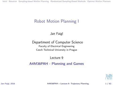
Robot Motion Planning – Motivational problemHow to transform high-level task specification (provided by humans)into a low-level description suitable for controlling the actuators?
To develop algorithms for such a transformation.
The motion planning algorithms provide transformations how tomove a robot (object) considering all operational constraints.
It encompasses several disciples, e.g., mathematics,robotics, computer science, control theory, artificialintelligence, computational geometry, etc.
Jan Faigl, 2016 A4M36PAH – Lecture 9: Trajectory Planning 5 / 62
Intro Notation Sampling-based Motion Planning Randomized Sampling-Based Methods Optimal Motion Planners
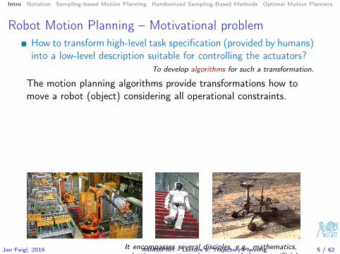
Piano Mover’s ProblemA classical motion planning problem
Having a CAD model of the piano, model of the environment, the prob-lem is how to move the piano from one place to another without hittinganything.
Basic motion planning algorithms are focused pri-marily on rotations and translations.
We need notion of model representations and formal definition ofthe problem.Moreover, we also need a context about the problem and realisticassumptions.
The plans have to be admissible and feasible.
Jan Faigl, 2016 A4M36PAH – Lecture 9: Trajectory Planning 6 / 62

Intro Notation Sampling-based Motion Planning Randomized Sampling-Based Methods Optimal Motion Planners
Robotic Planning Context
Pathrobot and
workspace
Models of
Trajectory Planning
Tasks and Actions Plans
Mission Planning
feedback control
Sensing and Acting
controller − drives (motors) − sensors
Trajectory
symbol level
"geometric" level
"physical" level
Problem Path Planning
Motion Planning
Sources of uncertainties
because of real environment
Open−loop control?
Robot Control
Jan Faigl, 2016 A4M36PAH – Lecture 9: Trajectory Planning 7 / 62

Intro Notation Sampling-based Motion Planning Randomized Sampling-Based Methods Optimal Motion Planners
Real Mobile Robots
In a real deployment, the problem is a more complex.
The world is changingRobots update the knowledge aboutthe environment
localization, mapping and navigation
New decisions have to madeA feedback from the environment
Motion planning is a part of the missionreplanning loop.
Josef Štrunc, Bachelorthesis, CTU, 2009.
An example of robotic mission:
Multi-robot exploration of unknown environment
How to deal with real-world complexity?Relaxing constraints and considering realistic assumptions.
Jan Faigl, 2016 A4M36PAH – Lecture 9: Trajectory Planning 8 / 62

Intro Notation Sampling-based Motion Planning Randomized Sampling-Based Methods Optimal Motion Planners
Notation
W – World model describes the robot workspace and its boundarydetermines the obstacles Oi .
2D world, W = R2
A Robot is defined by its geometry, parameters (kinematics) and itis controllable by the motion plan.C – Configuration space (C-space)A concept to describe possible configurations of the robot. Therobot’s configuration completely specify the robot location inWincluding specification of all degrees of freedom.
E.g., a robot with rigid body in a plane C = {x , y , ϕ} = R2 × S1.
Let A be a subset of W occupied by the robot, A = A(q).A subset of C occupied by obstacles is
Cobs = {q ∈ C : A(q) ∩ Oi ,∀i}
Collision-free configurations areCfree = C \ Cobs .
Jan Faigl, 2016 A4M36PAH – Lecture 9: Trajectory Planning 10 / 62
Intro Notation Sampling-based Motion Planning Randomized Sampling-Based Methods Optimal Motion Planners
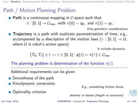
Path / Motion Planning ProblemPath is a continuous mapping in C-space such that
π : [0, 1]→ Cfree , with π(0) = q0, and π(1) = qf ,
Only geometric considerations
Trajectory is a path with explicate parametrization of time, e.g.,accompanied by a description of the motion laws (γ : [0, 1] → U ,where U is robot’s action space).
It includes dynamics.
[T0,Tf ] 3 t τ ∈ [0, 1] : q(t) = π(τ) ∈ Cfree
The planning problem is determination of the function π(·).
Additional requirements can be given:
Smoothness of the pathKinodynamic constraints
E.g., considering friction forces
Optimality criterionshortest vs fastest (length vs curvature)
Jan Faigl, 2016 A4M36PAH – Lecture 9: Trajectory Planning 11 / 62
Intro Notation Sampling-based Motion Planning Randomized Sampling-Based Methods Optimal Motion Planners
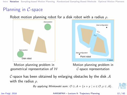
Planning in C-spaceRobot motion planning robot for a disk robot with a radius ρ.
Disk robot
Goal position
Start position
Motion planning problem ingeometrical representation of W
C−space
Cfree
Point robot
Start configuration
Goal configuration
obstC
Motion planning problem inC-space representation
C-space has been obtained by enlarging obstacles by the disk Awith the radius ρ.
By applying Minkowski sum: O ⊕A = {x + y | x ∈ O, y ∈ A}.
Jan Faigl, 2016 A4M36PAH – Lecture 9: Trajectory Planning 12 / 62

Intro Notation Sampling-based Motion Planning Randomized Sampling-Based Methods Optimal Motion Planners
Example of Cobs for a Robot with Rotation
x
y
θ
y
Robot body
Reference point
θ=π/2
θ=0 x
x
y
obsC
A simple 2D obstacle → has a complicated Cobs
Deterministic algorithms existRequires exponential time in C dimension,
J. Canny, PAMI, 8(2):200–209, 1986
Explicit representation of Cfree is impractical to compute.
Jan Faigl, 2016 A4M36PAH – Lecture 9: Trajectory Planning 13 / 62
Intro Notation Sampling-based Motion Planning Randomized Sampling-Based Methods Optimal Motion Planners
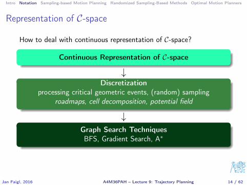
Representation of C-space
How to deal with continuous representation of C-space?
Continuous Representation of C-space
↓Discretization
processing critical geometric events, (random) samplingroadmaps, cell decomposition, potential field
↓Graph Search TechniquesBFS, Gradient Search, A∗
Jan Faigl, 2016 A4M36PAH – Lecture 9: Trajectory Planning 14 / 62
Intro Notation Sampling-based Motion Planning Randomized Sampling-Based Methods Optimal Motion Planners
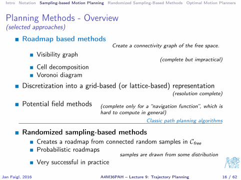
Planning Methods - Overview(selected approaches)
Roadmap based methodsCreate a connectivity graph of the free space.
Visibility graph(complete but impractical)
Cell decompositionVoronoi diagram
Discretization into a grid-based (or lattice-based) representation(resolution complete)
Potential field methods (complete only for a “navigation function”, which ishard to compute in general)
Classic path planning algorithms
Randomized sampling-based methodsCreates a roadmap from connected random samples in CfreeProbabilistic roadmaps
samples are drawn from some distributionVery successful in practice
Jan Faigl, 2016 A4M36PAH – Lecture 9: Trajectory Planning 16 / 62
Intro Notation Sampling-based Motion Planning Randomized Sampling-Based Methods Optimal Motion Planners
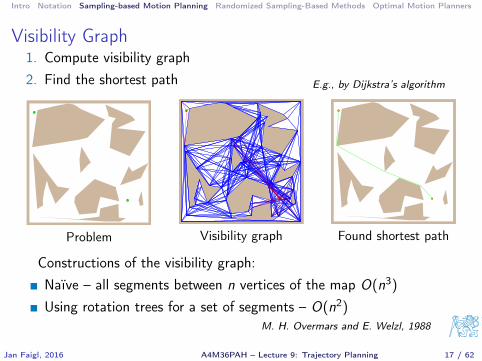
Visibility Graph1. Compute visibility graph2. Find the shortest path E.g., by Dijkstra’s algorithm
Problem Visibility graph Found shortest path
Constructions of the visibility graph:Naïve – all segments between n vertices of the map O(n3)
Using rotation trees for a set of segments – O(n2)M. H. Overmars and E. Welzl, 1988
Jan Faigl, 2016 A4M36PAH – Lecture 9: Trajectory Planning 17 / 62

Intro Notation Sampling-based Motion Planning Randomized Sampling-Based Methods Optimal Motion Planners
Voronoi Diagram
1. Roadmap is Voronoi diagram that maximizes clearance from theobstacles
2. Start and goal positions are connected to the graph3. Path is found using a graph search algorithm
Voronoi diagram Path in graph Found path
Jan Faigl, 2016 A4M36PAH – Lecture 9: Trajectory Planning 18 / 62
Intro Notation Sampling-based Motion Planning Randomized Sampling-Based Methods Optimal Motion Planners
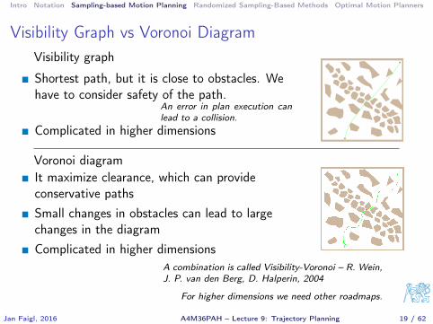
Visibility Graph vs Voronoi DiagramVisibility graph
Shortest path, but it is close to obstacles. Wehave to consider safety of the path.
An error in plan execution canlead to a collision.
Complicated in higher dimensions
Voronoi diagramIt maximize clearance, which can provideconservative pathsSmall changes in obstacles can lead to largechanges in the diagramComplicated in higher dimensions
A combination is called Visibility-Voronoi – R. Wein,J. P. van den Berg, D. Halperin, 2004
For higher dimensions we need other roadmaps.
Jan Faigl, 2016 A4M36PAH – Lecture 9: Trajectory Planning 19 / 62

Intro Notation Sampling-based Motion Planning Randomized Sampling-Based Methods Optimal Motion Planners
Cell Decomposition1. Decompose free space into parts.
Any two points in a convex region can be directlyconnected by a segment.
2. Create an adjacency graph representing the connectivity of thefree space.
3. Find a path in the graph.
Trapezoidal decomposition
Centroids representcells
Connect adjacencycells
q
gq
0
Find path in theadjacency graph
Other decomposition (e.g., triangulation) are possible.
Jan Faigl, 2016 A4M36PAH – Lecture 9: Trajectory Planning 20 / 62
Intro Notation Sampling-based Motion Planning Randomized Sampling-Based Methods Optimal Motion Planners
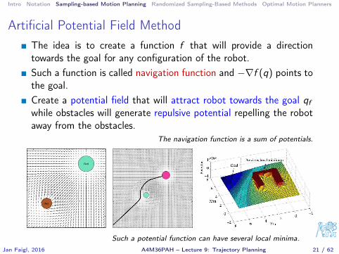
Artificial Potential Field MethodThe idea is to create a function f that will provide a directiontowards the goal for any configuration of the robot.Such a function is called navigation function and −∇f (q) points tothe goal.Create a potential field that will attract robot towards the goal qfwhile obstacles will generate repulsive potential repelling the robotaway from the obstacles.
The navigation function is a sum of potentials.
Such a potential function can have several local minima.Jan Faigl, 2016 A4M36PAH – Lecture 9: Trajectory Planning 21 / 62
Intro Notation Sampling-based Motion Planning Randomized Sampling-Based Methods Optimal Motion Planners
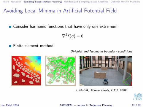
Avoiding Local Minima in Artificial Potential Field
Consider harmonic functions that have only one extremum
∇2f (q) = 0
Finite element methodDirichlet and Neumann boundary conditions
J. Mačák, Master thesis, CTU, 2009
Jan Faigl, 2016 A4M36PAH – Lecture 9: Trajectory Planning 22 / 62
Intro Notation Sampling-based Motion Planning Randomized Sampling-Based Methods Optimal Motion Planners
Sampling-based Motion Planning
Avoids explicit representation of the obstacles in C-spaceA “black-box” function is used to evaluate a configuration q is acollision free
(E.g., based on geometrical models and testingcollisions of the models)
It creates a discrete representation of CfreeConfigurations in Cfree are sampled randomly and connected to aroadmap (probabilistic roadmap)Rather than full completeness they provides probabilistic com-pleteness or resolution completeness
Probabilistic complete algorithms: with increasing number of samplesan admissible solution would be found (if exists)
Jan Faigl, 2016 A4M36PAH – Lecture 9: Trajectory Planning 24 / 62
Intro Notation Sampling-based Motion Planning Randomized Sampling-Based Methods Optimal Motion Planners
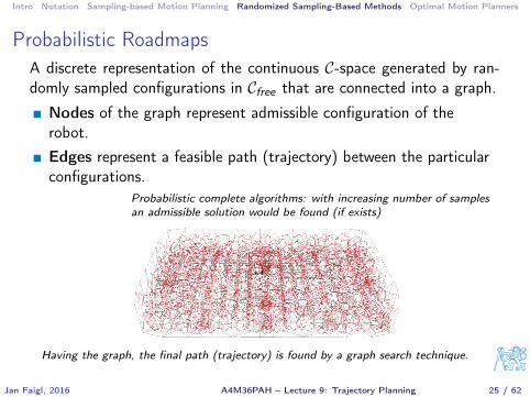
Probabilistic RoadmapsA discrete representation of the continuous C-space generated by ran-domly sampled configurations in Cfree that are connected into a graph.
Nodes of the graph represent admissible configuration of therobot.Edges represent a feasible path (trajectory) between the particularconfigurations.
Probabilistic complete algorithms: with increasing number of samplesan admissible solution would be found (if exists)
Having the graph, the final path (trajectory) is found by a graph search technique.
Jan Faigl, 2016 A4M36PAH – Lecture 9: Trajectory Planning 25 / 62

Intro Notation Sampling-based Motion Planning Randomized Sampling-Based Methods Optimal Motion Planners
Probabilistic Roadmap StrategiesMulti-QueryGenerate a single roadmap that is then used for planning queriesseveral times.An representative technique is Probabilistic RoadMap (PRM)
Probabilistic Roadmaps for Path Planning in High Dimensional ConfigurationSpacesLydia E. Kavraki and Petr Svestka and Jean-Claude Latombe and Mark H.Overmars,IEEE Transactions on Robotics and Automation, 12(4):566–580, 1996.
Single-QueryFor each planning problem constructs a new roadmap to character-ize the subspace of C-space that is relevant to the problem.
Rapidly-exploring Random Tree – RRT LaValle, 1998Expansive-Space Tree – EST Hsu et al., 1997Sampling-based Roadmap of Trees – SRT
(combination of multiple–query and single–query approaches)Plaku et al., 2005
Jan Faigl, 2016 A4M36PAH – Lecture 9: Trajectory Planning 26 / 62

Intro Notation Sampling-based Motion Planning Randomized Sampling-Based Methods Optimal Motion Planners
Multi-Query Strategy
Build a roadmap (graph) representing the environment1. Learning phase
1.1 Sample n points in Cfree1.2 Connect the random configurations using a local planner
2. Query phase2.1 Connect start and goal configurations with the PRM
E.g., using a local planner2.2 Use the graph search to find the path
Probabilistic Roadmaps for Path Planning in High Dimensional ConfigurationSpacesLydia E. Kavraki and Petr Svestka and Jean-Claude Latombe and Mark H.Overmars,IEEE Transactions on Robotics and Automation, 12(4):566–580, 1996.
First planner that demonstrates ability to solve general planning prob-lems in more than 4-5 dimensions.
Jan Faigl, 2016 A4M36PAH – Lecture 9: Trajectory Planning 27 / 62
Intro Notation Sampling-based Motion Planning Randomized Sampling-Based Methods Optimal Motion Planners
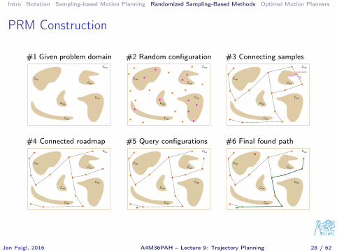
PRM Construction
#1 Given problem domain #2 Random configuration #3 Connecting samples
C
C
obs
obsC
free
C
obsC
obsC
obs
C
obsC
Cfree
obs
obs
Cobs
C
obsC
Local planner
C
Cobs
obsC
obs
freeC
Cobs
Cobs
collisionδ
#4 Connected roadmap #5 Query configurations #6 Final found path
C
freeC
Cobs
Cobs
Cobs
Cobs
obsC
freeC
Cobs
Cobs
Cobs
Cobs
obsC
freeC
Cobs
Cobs
Cobs
Cobs
obs
Jan Faigl, 2016 A4M36PAH – Lecture 9: Trajectory Planning 28 / 62

Intro Notation Sampling-based Motion Planning Randomized Sampling-Based Methods Optimal Motion Planners
Practical PRM
Incremental constructionConnect nodes in a radius ρLocal planner tests collisions upto selected resolution δPath can be found by Dijkstra’salgorithm
ρ
obs
obsC
obsC
obsC
Cfree
obs
C
C
What are the properties of the PRM algorithm?
We need a couple of more formalism.
Jan Faigl, 2016 A4M36PAH – Lecture 9: Trajectory Planning 29 / 62
Intro Notation Sampling-based Motion Planning Randomized Sampling-Based Methods Optimal Motion Planners
Path Planning Problem Formulation
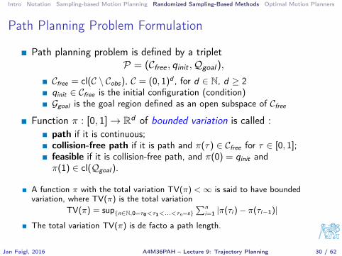
Path planning problem is defined by a tripletP = (Cfree , qinit ,Qgoal),
Cfree = cl(C \ Cobs), C = (0, 1)d , for d ∈ N, d ≥ 2qinit ∈ Cfree is the initial configuration (condition)Ggoal is the goal region defined as an open subspace of Cfree
Function π : [0, 1]→ Rd of bounded variation is called :path if it is continuous;collision-free path if it is path and π(τ) ∈ Cfree for τ ∈ [0, 1];feasible if it is collision-free path, and π(0) = qinit andπ(1) ∈ cl(Qgoal).
A function π with the total variation TV(π) <∞ is said to have boundedvariation, where TV(π) is the total variation
TV(π) = sup{n∈N,0=τ0<τ1<...<τn=s}∑n
i=1 |π(τi )− π(τi−1)|
The total variation TV(π) is de facto a path length.
Jan Faigl, 2016 A4M36PAH – Lecture 9: Trajectory Planning 30 / 62

Intro Notation Sampling-based Motion Planning Randomized Sampling-Based Methods Optimal Motion Planners
Path Planning Problem
Feasible path planning:For a path planning problem (Cfree , qinit ,Qgoal)
Find a feasible path π : [0, 1]→ Cfree such that π(0) = qinit andπ(1) ∈ cl(Qgoal), if such path exists.Report failure if no such path exists.
Optimal path planning:The optimality problem ask for a feasible path with the minimum cost.
For (Cfree , qinit ,Qgoal) and a cost function c : Σ→ R≥0Find a feasible path π∗ such thatc(π∗) = min{c(π) : π is feasible}.Report failure if no such path exists.
The cost function is assumed to be monotonic and bounded,i.e., there exists kc such that c(π) ≤ kc TV(π).
Jan Faigl, 2016 A4M36PAH – Lecture 9: Trajectory Planning 31 / 62

Intro Notation Sampling-based Motion Planning Randomized Sampling-Based Methods Optimal Motion Planners
Probabilistic Completeness 1/2
First, we need robustly feasible path planning problem(Cfree , qinit ,Qgoal).
q ∈ Cfree is δ-interior state of Cfree ifthe closed ball of radius δ centered at qlies entirely inside Cfree .
δ
q
−interior state
int ( )
obs
Cfreeδ
C
δ-interior of Cfree is intδ(Cfree) = {q ∈ Cfree |B/,δ ⊆ Cfree}.A collection of all δ-interior states.
A collision free path π has strong δ-clearance, if π lies entirelyinside intδ(Cfree).(Cfree , qinit ,Qgoal) is robustly feasible if a solution exists and it is afeasible path with strong δ-clearance, for δ>0.
Jan Faigl, 2016 A4M36PAH – Lecture 9: Trajectory Planning 32 / 62

Intro Notation Sampling-based Motion Planning Randomized Sampling-Based Methods Optimal Motion Planners
Probabilistic Completeness 2/2
An algorithmALG is probabilistically complete if, for any robustlyfeasible path planning problem P = (Cfree , qinit ,Qgoal)
limn→0
Pr(ALG returns a solution to P) = 1.
It is a “relaxed” notion of completenessApplicable only to problems with a robust solution.
C
C
obs
freeint ( )δ
init
Cobs
Cfreeδ
int ( )
q
We need some space, where random configurationscan be sampled
Jan Faigl, 2016 A4M36PAH – Lecture 9: Trajectory Planning 33 / 62

Intro Notation Sampling-based Motion Planning Randomized Sampling-Based Methods Optimal Motion Planners
Asymptotic Optimality 1/4
Asymptotic optimality relies on a notion of weak δ-clearanceNotice, we use strong δ-clearance for probabilistic completeness
Function ψ : [0, 1]→ Cfree is called homotopy, if ψ(0) = π1 and ψ(1) =π2 and ψ(τ) is collision-free path for all τ ∈ [0, 1].A collision-free path π1 is homotopic to π2 if there exists homotopyfunction ψ.
A path homotopic to π can be continuously trans-formed to π through Cfree .
Jan Faigl, 2016 A4M36PAH – Lecture 9: Trajectory Planning 34 / 62

Intro Notation Sampling-based Motion Planning Randomized Sampling-Based Methods Optimal Motion Planners
Asymptotic Optimality 2/4
A collision-free path π : [0, s] → Cfree has weak δ-clearance ifthere exists a path π′ that has strong δ-clearance and homotopyψ with ψ(0) = π, ψ(1) = π′, and for all α ∈ (0, 1] there existsδα > 0 such that ψ(α) has strong δ-clearance.
Weak δ-clearance does not require points along apath to be at least a distance δ away from obstacles.
π
π’init
obs
Cfreeδ
int ( )
q
C A path π with a weak δ-clearanceπ′ lies in intδ(Cfree) and it is thesame homotopy class as π
Jan Faigl, 2016 A4M36PAH – Lecture 9: Trajectory Planning 35 / 62
Intro Notation Sampling-based Motion Planning Randomized Sampling-Based Methods Optimal Motion Planners
Asymptotic Optimality 3/4
It is applicable with a robust optimal solution that can be obtainedas a limit of robust (non-optimal) solutions.A collision-free path π∗ is robustly optimal solution if it has weakδ-clearance and for any sequence of collision free paths {πn}n∈N,πn ∈ Cfree such that limn→∞ πn = π∗,
limn→∞
c(πn) = c(π∗).
There exists a path with strong δ-clearance, and π∗ ishomotopic to such path and π∗ is of the lower cost.
Weak δ-clearance implies robustly feasible solution problem(thus, probabilistic completeness)
Jan Faigl, 2016 A4M36PAH – Lecture 9: Trajectory Planning 36 / 62
Intro Notation Sampling-based Motion Planning Randomized Sampling-Based Methods Optimal Motion Planners
Asymptotic Optimality 4/4
An algorithm ALG is asymptotically optimal if, for any path plan-ning problem P = (Cfree , qinit ,Qgoal) and cost function c that admita robust optimal solution with the finite cost c∗
Pr
({limi→∞
YALGi = c∗})
= 1.
YALGi is the extended random variable corresponding to the minimum-cost solution included in the graph returned by ALG at the end ofiteration i .
Jan Faigl, 2016 A4M36PAH – Lecture 9: Trajectory Planning 37 / 62

Intro Notation Sampling-based Motion Planning Randomized Sampling-Based Methods Optimal Motion Planners
Properties of the PRM Algorithm
Completeness for the standard PRM has not been provided whenit was introducedA simplified version of the PRM (called sPRM) has been mostlystudiedsPRM is probabilistically complete
What are the differences between PRM and sPRM?
Jan Faigl, 2016 A4M36PAH – Lecture 9: Trajectory Planning 38 / 62
Intro Notation Sampling-based Motion Planning Randomized Sampling-Based Methods Optimal Motion Planners
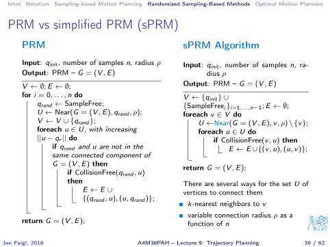
PRM vs simplified PRM (sPRM)PRM
Input: qinit , number of samples n, radius ρOutput: PRM – G = (V ,E)
V ← ∅;E ← ∅;for i = 0, . . . , n do
qrand ← SampleFree;U ← Near(G = (V ,E), qrand , ρ);V ← V ∪ {qrand};foreach u ∈ U, with increasing||u − qr || do
if qrand and u are not in thesame connected component ofG = (V ,E) then
if CollisionFree(qrand , u)then
E ← E ∪{(qrand , u), (u, qrand )};
return G = (V ,E);
sPRM Algorithm
Input: qinit , number of samples n, ra-dius ρ
Output: PRM – G = (V ,E)
V ← {qinit} ∪{SampleFreei}i=1,...,n−1;E ← ∅;foreach v ∈ V do
U ←Near(G = (V ,E), v , ρ) \ {v};foreach u ∈ U do
if CollisionFree(v , u) thenE ← E ∪{(v , u), (u, v)};
return G = (V ,E);
There are several ways for the set U ofvertices to connect them
k-nearest neighbors to v
variable connection radius ρ as afunction of n
Jan Faigl, 2016 A4M36PAH – Lecture 9: Trajectory Planning 39 / 62

Intro Notation Sampling-based Motion Planning Randomized Sampling-Based Methods Optimal Motion Planners
PRM – Properties
sPRM (simplified PRM)Probabilistically complete and asymptotically optimalProcessing complexity O(n2)Query complexity O(n2)Space complexity O(n2)
Heuristics practically used are usually not probabilistic completek-nearest sPRM is not probabilistically completevariable radius sPRM is not probabilistically complete
Based on analysis of Karaman and Frazzoli
PRM algorithm:+ Has very simple implementation+ Completeness (for sPRM)− Differential constraints (car-like vehicles) are not straightforward
Jan Faigl, 2016 A4M36PAH – Lecture 9: Trajectory Planning 40 / 62

Intro Notation Sampling-based Motion Planning Randomized Sampling-Based Methods Optimal Motion Planners
Comments about Random Sampling 1/2
Different sampling strategies (distributions) may be applied
Notice, one of the main issue of the randomized sampling-basedapproaches is the narrow passageSeveral modifications of sampling based strategies have been pro-posed in the last decades
Jan Faigl, 2016 A4M36PAH – Lecture 9: Trajectory Planning 41 / 62
Intro Notation Sampling-based Motion Planning Randomized Sampling-Based Methods Optimal Motion Planners
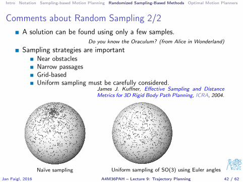
Comments about Random Sampling 2/2A solution can be found using only a few samples.
Do you know the Oraculum? (from Alice in Wonderland)
Sampling strategies are importantNear obstaclesNarrow passagesGrid-basedUniform sampling must be carefully considered.
James J. Kuffner, Effective Sampling and DistanceMetrics for 3D Rigid Body Path Planning, ICRA, 2004.
Naïve sampling Uniform sampling of SO(3) using Euler angles
Jan Faigl, 2016 A4M36PAH – Lecture 9: Trajectory Planning 42 / 62
Intro Notation Sampling-based Motion Planning Randomized Sampling-Based Methods Optimal Motion Planners
Rapidly Exploring Random Tree (RRT)
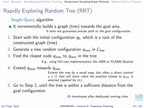
Single–Query algorithmIt incrementally builds a graph (tree) towards the goal area.
It does not guarantee precise path to the goal configuration.
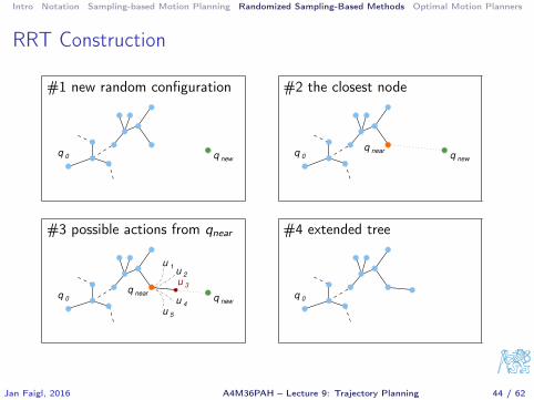
1. Start with the initial configuration q0, which is a root of theconstructed graph (tree)
2. Generate a new random configuration qnew in Cfree3. Find the closest node qnear to qnew in the tree
E.g., using KD-tree implementation like ANN or FLANN libraries
4. Extend qnear towards qnewExtend the tree by a small step, but often a direct controlu ∈ U that will move robot the position closest to qnew isselected (applied for δt).
5. Go to Step 2, until the tree is within a sufficient distance from thegoal configuration
Or terminates after dedicated running time.
Jan Faigl, 2016 A4M36PAH – Lecture 9: Trajectory Planning 43 / 62
Intro Notation Sampling-based Motion Planning Randomized Sampling-Based Methods Optimal Motion Planners
RRT Construction
#1 new random configuration
0 q newq
#2 the closest node
0
q nearq new
q
#3 possible actions from qnear
new
u 3
u 5
u 4
u 2
u 1
q nearq0q
#4 extended tree
q 0
Jan Faigl, 2016 A4M36PAH – Lecture 9: Trajectory Planning 44 / 62

Intro Notation Sampling-based Motion Planning Randomized Sampling-Based Methods Optimal Motion Planners
RRT AlgorithmMotivation is a single query and control-based path findingIt incrementally builds a graph (tree) towards the goal area.
RRT AlgorithmInput: qinit , number of samples n
Output: Roadmap G = (V ,E)
V ← {qinit};E ← ∅;for i = 1, . . . , n do
qrand ← SampleFree;qnearest ← Nearest(G = (V ,E), qrand );qnew ← Steer(qnearest , qrand );if CollisionFree(qnearest , qnew ) then
V ← V ∪ {xnew}; E ← E ∪ {(xnearest , xnew )};
return G = (V ,E);
Extend the tree by a small step, but often a direct control u ∈ U that willmove robot to the position closest to qnew is selected (applied for dt).
Rapidly-exploring random trees: A new tool for path planningS. M. LaValle,Technical Report 98-11, Computer Science Dept., Iowa State University, 1998
Jan Faigl, 2016 A4M36PAH – Lecture 9: Trajectory Planning 45 / 62
Intro Notation Sampling-based Motion Planning Randomized Sampling-Based Methods Optimal Motion Planners
Properties of RRT Algorithms
Rapidly explores the spaceqnew will more likely be generated in large not yet covered parts.
Allows considering kinodynamic/dynamic constraints (during theexpansion).Can provide trajectory or a sequence of direct control commandsfor robot controllers.A collision detection test is usually used as a “black-box”.
E.g., RAPID, Bullet libraries.
Similarly to PRM, RRT algorithms have poor performance innarrow passage problems.RRT algorithms provides feasible paths.
It can be relatively far from optimal solution, e.g.,according to the length of the path.
Many variants of RRT have been proposed.
Jan Faigl, 2016 A4M36PAH – Lecture 9: Trajectory Planning 46 / 62

Intro Notation Sampling-based Motion Planning Randomized Sampling-Based Methods Optimal Motion Planners
RRT – Examples 1/2
Alpha puzzle benchmark Apply rotations to reach the goal
Bugtrap benchmark Variants of RRT algorithmsCourtesy of V. Vonásek and P. Vaněk
Jan Faigl, 2016 A4M36PAH – Lecture 9: Trajectory Planning 47 / 62
Intro Notation Sampling-based Motion Planning Randomized Sampling-Based Methods Optimal Motion Planners
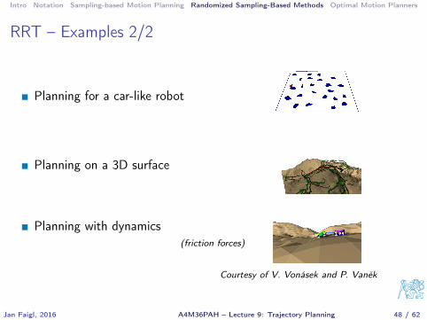
RRT – Examples 2/2
Planning for a car-like robot
Planning on a 3D surface
Planning with dynamics(friction forces)
Courtesy of V. Vonásek and P. Vaněk
Jan Faigl, 2016 A4M36PAH – Lecture 9: Trajectory Planning 48 / 62

Intro Notation Sampling-based Motion Planning Randomized Sampling-Based Methods Optimal Motion Planners
Car-Like Robot
Configuration
−→x =
xyφ
position and orientation
Controls−→u =
(vϕ
)forward velocity, steering angle
System equationx = v cosφy = v sinφ
ϕ =v
Ltanϕ
(x, y)
L
θ
ϕ
ICC
Kinematic constraints dim(−→u ) < dim(−→x )
Differential constraints on possible q:
x sin(φ)− y cos(φ) = 0
Jan Faigl, 2016 A4M36PAH – Lecture 9: Trajectory Planning 49 / 62

Intro Notation Sampling-based Motion Planning Randomized Sampling-Based Methods Optimal Motion Planners
Control-Based Sampling
Select a configuration q from the tree T of the currentconfigurations
Pick a control input −→u = (v , ϕ) andintegrate system (motion) equationover a short period ∆x
∆y∆ϕ
=
∫t+∆t
t
v cosφv sinφvL tanϕ
dt
If the motion is collision-free, add the endpoint to the tree
E.g., considering k configurations for kδt = dt.
Jan Faigl, 2016 A4M36PAH – Lecture 9: Trajectory Planning 50 / 62
Intro Notation Sampling-based Motion Planning Randomized Sampling-Based Methods Optimal Motion Planners
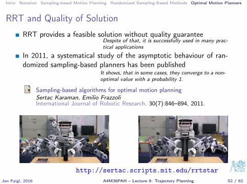
RRT and Quality of Solution
RRT provides a feasible solution without quality guaranteeDespite of that, it is successfully used in many prac-tical applications
In 2011, a systematical study of the asymptotic behaviour of ran-domized sampling-based planners has been published
It shows, that in some cases, they converge to a non-optimal value with a probability 1.
Sampling-based algorithms for optimal motion planningSertac Karaman, Emilio FrazzoliInternational Journal of Robotic Research, 30(7):846–894, 2011.
http://sertac.scripts.mit.edu/rrtstarJan Faigl, 2016 A4M36PAH – Lecture 9: Trajectory Planning 52 / 62
Intro Notation Sampling-based Motion Planning Randomized Sampling-Based Methods Optimal Motion Planners
RRT and Quality of Solution 1/2
Let Y RRTi be the cost of the best path in the RRT at the end of
iteration i .Y RRTi converges to a random variable
limi→∞
Y RRTi = Y RRT
∞ .
The random variable Y RRT∞ is sampled from a distribution with zero
mass at the optimum, and
Pr [Y RRT∞ > c∗] = 1.
Karaman and Frazzoli, 2011
The best path in the RRT converges to a sub-optimal solution al-most surely.
Jan Faigl, 2016 A4M36PAH – Lecture 9: Trajectory Planning 53 / 62

Intro Notation Sampling-based Motion Planning Randomized Sampling-Based Methods Optimal Motion Planners
RRT and Quality of Solution 2/2
RRT does not satify a necessary condition for the asymptotic opti-mality
For 0 < R < infq∈Qgoal||q− qinit ||, the event {limn→∞ Y RTT
n = c∗}occurs only if the k-th branch of the RRT contains vertices outsidethe R-ball centered at qinit for infinitely many k .
See Appendix B in Karaman&Frazzoli, 2011
It is required the root node will have infinitely many subtrees thatextend at least a distance ε away from qinit
The sub-optimality is caused by disallowing new better pathsto be discovered.
Jan Faigl, 2016 A4M36PAH – Lecture 9: Trajectory Planning 54 / 62
Intro Notation Sampling-based Motion Planning Randomized Sampling-Based Methods Optimal Motion Planners
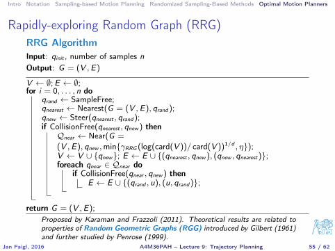
Rapidly-exploring Random Graph (RRG)RRG AlgorithmInput: qinit , number of samples nOutput: G = (V ,E)
V ← ∅;E ← ∅;for i = 0, . . . , n do
qrand ← SampleFree;qnearest ← Nearest(G = (V ,E), qrand);qnew ← Steer(qnearest , qrand);if CollisionFree(qnearest , qnew ) thenQnear ← Near(G =
(V ,E), qnew ,min{γRRG (log(card(V ))/ card(V ))1/d , η});V ← V ∪ {qnew}; E ← E ∪ {(qnearest , qnew ), (qnew , qnearest)};foreach qnear ∈ Qnear do
if CollisionFree(qnear , qnew ) thenE ← E ∪ {(qrand , u), (u, qrand)};
return G = (V ,E);Proposed by Karaman and Frazzoli (2011). Theoretical results are related toproperties of Random Geometric Graphs (RGG) introduced by Gilbert (1961)and further studied by Penrose (1999).
Jan Faigl, 2016 A4M36PAH – Lecture 9: Trajectory Planning 55 / 62
Intro Notation Sampling-based Motion Planning Randomized Sampling-Based Methods Optimal Motion Planners
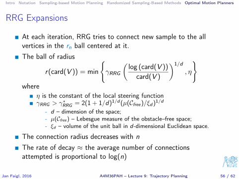
RRG Expansions
At each iteration, RRG tries to connect new sample to the allvertices in the rn ball centered at it.The ball of radius
r(card(V )) = min
{γRRG
(log (card(V ))
card(V )
)1/d
, η
}where
η is the constant of the local steering functionγRRG > γ∗RRG = 2(1 + 1/d)1/d(µ(Cfree)/ξd)1/d
- d – dimension of the space;- µ(Cfree) – Lebesgue measure of the obstacle–free space;- ξd – volume of the unit ball in d-dimensional Euclidean space.
The connection radius decreases with n
The rate of decay ≈ the average number of connectionsattempted is proportional to log(n)
Jan Faigl, 2016 A4M36PAH – Lecture 9: Trajectory Planning 56 / 62
Intro Notation Sampling-based Motion Planning Randomized Sampling-Based Methods Optimal Motion Planners
RRG Properties
Probabilistically completeAsymptotically optimalComplexity is O(log n)
(per one sample)
Computational efficiency and optimality
Attempt connection to Θ(log n) nodes at each iteration;in average
Reduce volume of the “connection” ball as log(n)/n;Increase the number of connections as log(n).
Jan Faigl, 2016 A4M36PAH – Lecture 9: Trajectory Planning 57 / 62
Intro Notation Sampling-based Motion Planning Randomized Sampling-Based Methods Optimal Motion Planners
Other Variants of the Optimal Motion Planning
PRM* – it follows standard PRM algorithm where connections areattempted between roadmap vertices that are within connectionradius r as a function of n
r(n) = γPRM(log(n)/n)1/d
RRT* – a modification of the RRG, where cycles are avoidedA tree version of the RRG
A tree roadmap allows to consider non-holonomic dynamics andkinodynamic constraints.It is basically RRG with “rerouting” the tree when a better path isdiscovered.
Jan Faigl, 2016 A4M36PAH – Lecture 9: Trajectory Planning 58 / 62
Intro Notation Sampling-based Motion Planning Randomized Sampling-Based Methods Optimal Motion Planners
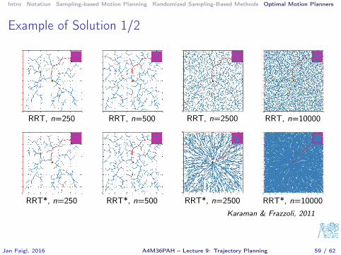
Example of Solution 1/2
RRT, n=250
RRT*, n=250
RRT, n=500
RRT*, n=500
RRT, n=2500
RRT*, n=2500
RRT, n=10000
RRT*, n=10000Karaman & Frazzoli, 2011
Jan Faigl, 2016 A4M36PAH – Lecture 9: Trajectory Planning 59 / 62
Intro Notation Sampling-based Motion Planning Randomized Sampling-Based Methods Optimal Motion Planners
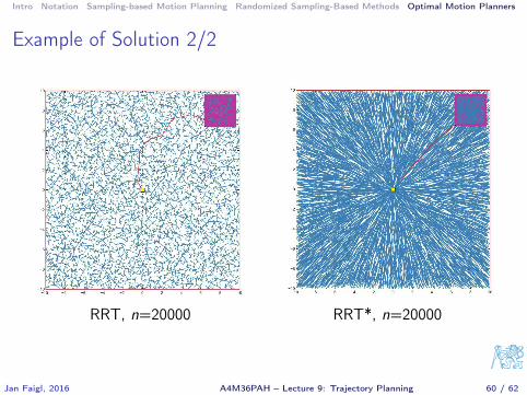
Example of Solution 2/2
RRT, n=20000 RRT*, n=20000
Jan Faigl, 2016 A4M36PAH – Lecture 9: Trajectory Planning 60 / 62
Intro Notation Sampling-based Motion Planning Randomized Sampling-Based Methods Optimal Motion Planners
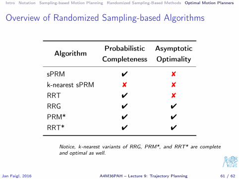
Overview of Randomized Sampling-based Algorithms
AlgorithmProbabilistic AsymptoticCompleteness Optimality
sPRM 4 8
k-nearest sPRM 8 8
RRT 4 8
RRG 4 4
PRM* 4 4
RRT* 4 4
Notice, k-nearest variants of RRG, PRM*, and RRT* are completeand optimal as well.
Jan Faigl, 2016 A4M36PAH – Lecture 9: Trajectory Planning 61 / 62
Intro Notation Sampling-based Motion Planning Randomized Sampling-Based Methods Optimal Motion Planners
Summary
Introduction to motion planningOverview of sampling-based planning methods
Basic roadmap methodsVisibility graphVoronoi diagramCell decomposition
Artificial potential field method
Randomized Sampling-based Methods and their properties (PRM,sPRM, RRT)Optimal Motion Planners (RRG, PRM∗, RRT∗)
Jan Faigl, 2016 A4M36PAH – Lecture 9: Trajectory Planning 62 / 62