Riverine Landscape of the Middle Platte River: Hydrological Connectivity and Physicochemical Heterogeneity
by
Wanli Wu
A DISSERTATION
Presented to the Faculty of
The Graduate College at the University of Nebraska
In Partial Fulfillment of Requirements
For the Degree of Doctor of Philosophy
Major: Natural Resource Sciences
Under the Supervision of Professor Kyle D. Hoagland
Lincoln, Nebraska
April 2003

DISSERTATION TITLE
Riverine Landscape of the Middle Platte River: Hydrological
Connectivity and Physicochemical Heterogenity
Wanli
SUPERVISORY COMMITTEE:
Approved
Signatue
Kyle D. Hoagland Typed Name
. 0
Gary L. Hergenrader Typed Name
Signature .
Darryl] T. pederson
Signature
Vjta]y A. Zlotnjk Typed Name
Signature
Typed Name
Signature
Typed Name
BY
Wu
Date
N ~'VERS'TY 1°.!-.. \ GRADUATE eUtasM COLLEGE

Riverine Landscape of the Middle Platte River:
Hydrological Connectivity and Physicochemical Heterogeneity
Wanli Wu, Ph.D.
University of Nebraska, 2003
Adviser: Kyle D. Hoagland
Fluvial processes create diverse riverine habitats and sustain hydrological
connectivity across broad floodplains of the Middle Platte River. The riverine habitats
have hierarchical characteristics and distinctive temporal variability. River regulation
reduces the hydrologic fluctuation and the degree of surface hydrological connectivity
between the river flow and the riverine habitats in the floodplain.
Two fundamental questions are: (a) how does hydrology of riverine habitats respond
to river discharge? (b) what are the riverine landscape patterns as results ofthe
hydrological change? It was hypothesized that discharge and hydrological connectivity
are the main factors controlling diversity of the riverine habitats and patterns of the
riverine landscape.
The hydrological connectivity was determined by quantifying hydrological
connections and interactions between the riverine habitats and the main channel in
landscape scale. Multiple correlation and regression methods were used to quantify the
1

hydrological interactions. The results suggest a rank of the hydrological connectivity
between the riverine habitats and the main channel (from high to low) as: side-channel,
disconnected backwater, connected backwater, wet meadow pond, riparian pond,
tributary, permanent slough, and intermittent slough.
Physicochemical and spatial analysis results reveal the riverine habitat heterogeneity
and landscape patterns in response to the river discharge. The hydrological connectivity
serves as a driving force for biodiversity of the river ecosystem. Thus, an effective
biodiversity conservation strategy should focus on sustaining hydrological connectivity,
so that the river itself may maintain its braided flowpaths and maintain hydrologic and
ecologic interactions among riverine landscape components.
11
This research contributes to our understanding of the complexity of the riverine
landscape in the Middle Platte River. It is also relevant to a fundamental question: how
does the hydrological connectivity affect the river ecosystems? The study results (The
landscape digital maps, hydrological and physicochemical data) show clearly the riverine
landscape patterns and the effects of hydrological and climatic factors on the landscape
processes. These results may serve for river ecosystem assessment, planning, habitat
conservation and restoration, and water resources management.

111
Acknowledgments
I am greatly indebted to my advisor,. Dr. Kyle Hoagland, and my former advisor, Dr.
Dennis Jelinski, for their full support, guidance, and enthusiastic encouragement during
my fieldwork and study. I am grateful to all of the professors on my Ph.D. supervisory
committee (Dr. Gary L. Hergenrader, Dr. Kyle D. Hoagland, Dr. Darryll T. Pederson, and
Dr. Vitaly A. Zlotnik) for their thorough examination of the project design and processes,
as well as the draft of my dissertation and improvement of its language and clarity. I
acknowledge financial support for this project from the School of Natural Resources
Sciences (formerly Department of Forestry, Fisheries and Wildlife) at the University of
Nebraska-Lincoln, the U.S. Environmental Protection Agency, and the U.S. Fish and
Wildlife Service. I also want to thank those agencies, organizations, and private
landowners who provided access to their properties or managed areas for this large-scale
field research, including the National Audubon Society-Lillian Annette Rowe Sanctuary,
The Nature Conservancy, the Nebraska Public Power District, the Platte River Whooping
Crane Maintenance Trust, Inc., the U.S. Fish and Wildlife Service at Grand Island, and
local farmers whose crop fields were adjacent to my research areas. I thank the
Department of Agronomy at University of Nebraska-Lincoln, and the Department of
Biology at Trent University in Peterborough, Ontario, Canada, for assisting in physical
and chemical analysis of the water and soil samples. Special thanks go to all of my field
assistants and volunteers: A. Carr, E. Carruthers, L. Fournier, J. Karagatzides, C. King, J.

IV
Leski, A. Meulen, R. Steinauer, and others for their outstanding help in my intensive
hydrologic monitoring and landscape survey. Important, too, was the role of Robert
Steinauer for his plant identifications and work on vegetation surveys. Also, Mike
Bullerman, Chris Colt, Chris Helzer, Tammy Vercauteren, and others provided help and
field-guidance during the initial period of my field survey. Without their tremendous
effort, this research could not be accomplished. I express my gratitude to Dave Carlson,
Paul Currier, Beth Goldowitz, Robert Henszey, Huihua Huang, Carter Johnson, Dan Li,
Wei Li, Gary Lingle, Tamera Minnick, Kent Pfeiffer, Paul Tebbel, Xinhao Wang, Fujiang
Wen, Hong Wu, Yi Zhang, and others who have helped me with the academic, technical,
and administrative aspects of the research, as well as my study, both in the field and on
campus. I sincerely appreciate the warm help and great care for my family and me from
the family of Marylyn and Dale Rowe since I came to Lincoln, Nebraska. Finally, I owe
very much to my parents and my family. Their concern and understanding accompanied
me through all of the seasons of my field work and study at the University of Nebraska
Lincoln.

v
Table of Contents
Abstract ............. .. .. . .................... . ................... .. .... . . . .. ... .... .. .......... . .. i Acknowledgements ..... .. .. . ....... .. ..... . . . ... . ............... . .. . ............ . . . ........... .. iii Table of Contents .................... .. ............ . .............. . .............................. v List of Figures ..... . ................ . .............. ... ......................... ... ............. ... viii List of Tables .................................................................................... xv
Chapter 1. Introduction .............. . ............................. . ......................... 1
1.1 Ecological significance of the riverine landscape in the Middle Platte River... ... I 1.2 Biodiversity of the floodplain river ecosystems... . ..... ......... . . . ... .. . ... ... . ...... 2 1.3 Hydrological influence to the riverine landscape and the biodiversity . .......... . ... 3 1.4 Research questions, goals, and objectives ............................................... 5
Chapter 2. Review of Theories and Approaches to the Riverine Landscape ....... 7
2.1 Basic theories of ecological approach to streams and rivers... ............... ........ 7 2.1.1 The river-continuum concept ........................................... . .. ; ...... 7 2.1.2 The flood-pulse concept ........................................................... 8 2.1.3 Hyporheic zone and groundwater/surface water ecotone ..................... 9
2.2 Hydrogeological approach to the stream-aquifer interaction .......................... 11 2.2.1 Control factors on the river-aquifer interaction and groundwater flow
systems . . ... ...................................................................... ..... 12 2.2.2 Mechanism of the stream-aquifer interaction ................................... 14 2.2.3 Hydrogeologic research on the Middle Platte River ........................... 15
2.3 The Riverine landscape -- a holistic perspective... ... ... ... . .... . ... . ..... ..... . ... ... 18 2.3.1 Concept of the riverine landscape ....................... .. .. . ... . ................ 19 2.3 .2 Diversity of riverine habitats .... . ... . ........... . ... . . ... .. .. .. .. ....... . . . ....... 20
2.4 Research design ................................. ... ......................................... 21 2.4.1 The hierarchical patch dynamic research framework .......................... 21 2.4.2 The conceptual model of the braided riverine landscape ...................... 22 2.4.3 Hydro-geomorphological approaches to the riverine landscape .............. 25 2.4.4 Physical principles of the riverine hydrologic processes ...................... 28 2.4.5 Research assumptions .............................................................. 31
Chapter 3. Methodology ............... .............. .. ....................................... 34
3.1 Study areas . . .... . . ......... .... .... ...... ......................... ..... . .. ... ... ............. 34 3.2 Data sets ............................. .... ................................... . ..... . ........... 39

VI
3.2.1 Hydrological data ................................................................... 39 3.2.2 Weather and climate data .......................................................... 40 3.2.3 Soil/Sediment and land cover data ...................... ............. . .......... .. 40 3.2.4 Surface water physicochemical data.. . . . . . . . . . . . . . . . . . . . . . . . . . . . . . . . . . . . . . . . . . .. 41 3.2.5 Spatial imagery data ... . .. . ............... . .................................... . .... 43
3.3 Methods.......................... . ..................................... . .... . ................ 44 3.3.1 Hydro-geomorphological classification ofthe aquatic habitats ............... 44 3.3.2 Correlation analysis on the main channel-riverine habitat interactions ...... 49 3.3.3 Cluster analysis on spatial pattern of the riverine habitat types ............... 51 3.3.4 Regression analyses ofthe main-channel discharges-riverine water levels 52 3.3.5 Analysis of variances on heterogeneity of physicochemical data ............ 54 3.3.6 Spatially explicit models of the riverine landscape ............................ 55
Chapter 4. Results and Discussions (I): Hydrological Connectivity . . . ... ......... .. 57
4.1 Surface hydrological connection and classification of the aquatic habitats ......... 57 4.2 Correlation between the main channel and the riverine habitats ............... 60 4.3 Stream widths and habitat locations on the stream-riverine habitat
correlations ............................................................ . ............... 67 4.4 Statistical modeling of the stream-riverine habitat interaction ................. . 73 4.4.1 Modeling water level change by the main channel discharge ................. 73 4.4.2 Stepwise multivariate regression models ................. . ...................... 78
4.5 Spatial patterns of the riverine landscape as response to hydrological changes .... 82 4.5.1 Components of the riverine landscape ............... . . . . . .... . .................. 82 4.5.2 Spatial analysis of the riverine hydrological patterns .......................... 85 4.5.3 Spatial analysis of the riverine habitat patterns ................................. 86
Chapter 5. Results and Discussions (II): Physicochemical Heterogeneity ........ .. 93
5.1 Physical and chemical properties of surface water in riverine landscape ........... . 94 5.1.1 Daytime temperature ........... . ... . . . ......................... . ................. . . 94 5.1.2 pH .................. .................................................................. 101 5.1.3 Dissolved oxygen ................ . .. . . . ................... . . . . . ..................... 107 5.1.4 Specific conductance ......................... ...................................... 112 5.1.5 Salinity ................................................................. . ............. 118
5.2 Nutrients of surface water in the riverine landscape .................................... 123 5.2.1 Nitrogen (N03-N and N02-N) ............... . .................. . ..... . .... . ...... 123 5.2.2 Ammonium (NH4-N) ........ . ....... .. .. . .. . ...... . .. . ............................. 131 5.2.3 Phosphate (P04-P) .................................... . ............................. 136
5.3 Major dissolved ions of surface water in the riverine landscape ..................... 141 5.3.1 Calcium (Ca2+) .................. ........................... ......................... 141

Vll
5.3.2 Magnesium (Mg2+) .. .. ...... . .. . .. . ....... . ..... . .... .. .. . ... ... ..... . . . ..... . ..... 147 5.3.3 Potassium (K+) ..... . .. . .......... . . . ................. . ................. .. . . ......... . 152 5.3.4 Sodium (Na+) ........... . .............................................. . . . ........... 157 5.3.5 Chloride (Cr) .... . ..................... . .. .. ...... .. ........... . ...... . . . . ... ........ 162 5.3.6 Sulfate (S042-) . ....... .. ....... . .. .. .... . ................................. . .......... 167
5.4 Trace elements of surface water in the riverine landscape . . .......... . ....... . ....... 172 5.5 Summary ...... . .... . . . ........ . .............. . ... . ........ . ........... . ........ . . . ... .. ...... 179
Chapter 6. Major findings and conclusions .... . .. . ........ .. ....... . . . ....... . ....... . .. 184
6.1 On the hydrological connectivity... ... ... ... . .......... . ......... ......... .... . . . ........ 184 6.1.1 Identification of hydrological connection in divers riverine habitat types.. 184 6.1.2 Quantification of the hydrological interactions in the riverine landscape.. 185 6.1.3 Relative importance of the climatic factors to the riverine habitats... ...... 186 6.1.4 Spatial patterns and dynamics of the riverine habitats ... . ......... . ..... . ...... 187
6.2 On the physicochemical heterogeneity. . .... . . . .......... . .... ......... ... ... .......... . 187 6.3 Research limitations and recommendations for future studies ... . ... . . . ... . . . ........ 189
6.3.1 Limitations in this study .. ................. . ... . ..... .... ............ . .... ..... . 189 6.3.2 Recommendations for future studies .......... . .......... . ....... .. . . . . ..... .. 190
Literature Cited . . ................... . . . ..... .. .. . ... . .......... . ...... . ......... . . . . . ... . . .. ... 192
Appendixes .............. . ......... . ........... . .................. . .............................. 213 A. List of the study areas, transects, and monitoring sites ........... .. ... .. .... . ..... . .... 213 B. Geographic locations and soil/sediment features ofthe study sites ...... .... .......... 215 C. Hydrographs of the studied sites (listed in order of the transects) ........... . .... . .... 216 D. Results of Statistical Analyses ........ .. . . ........... . .... . ..... . ... . .... . ........... ... ... 261

Figure 2-1.
Figure 2-2:
Figure 3-1.
Figure 3-2.
Figure 4-1.
Figure 4-2.
Figure 4-3.
Figure 4-4.
Figure 4-5.
Figure 4-6.
Vlll
List of Figures
Conceptual model of a braided riverine landscape. The question 23 symbols indicate those "hot spots" for studying the hydrological connectivity. Design of hydrologic monitoring network at study area 13, about 4.5 km southeast of Kearney, Nebraska..... . ........................ 27
Location of the study areas, USGS' stream gauging stations, and weather stations along the Middle Platte River...... . ............. .... 35
Land cover of a reach of Middle Platte River floodplain, about 4.5 km southeast of Kearney, Nebraska.................................... 38
Hierarchy of the aquatic habitat classification in the Middle Platte River floodplain........................................................ .... 59
Comparison of the mean correlation coefficients (Kendall's '[values, (l = 0.05) for water level changes between the main channel and the riverine habitat subtypes . . .. . .............. . ... .. .. . . .. ......... 64
Illustration of the riverine habitat hydrological connectivity with the main channel in the Middle Platte River. . . . . . . . . . . . . . . . . . . . . . . . . . . 66
Clustered riverine habitats by the habitat types, and the habitat surface water 1: values fit by the square root of the location parameter [Lr = (d+w/2)/w] ..................... . ........... . ......... .... 69
Clustered riverine habitats by the habitat types, and the habitat groundwater 1: values fit by the square root of the location parameter [Lr = (d+w/2)/w] . ..................................... . ........ 70
Land cover map exported from a GIS based digital riverine landscape classification model that covers a management property and adjacent areas at a reach of the Middle Platte River, 4 km southeast of Kearney, Nebraska. Original color infrared photograph was taken by U.S. FWS (1995) on October 25, 1995, when Q =
56.6 m3/s (2,000 cfs), representing a high instream flow management scenario . . .. . .................................... .. ........... 83

Figure 4-7. Land cover map exported from a GIS based digital riverine landscape classification model that covers a management property and adjacent areas at a reach of the Middle Platte River, 4 km southeast of Kearney, Nebraska. The original color infrared photograph was taken by U.S.G.S. (1998) on August 1998, when Q = 11.5 m3/s (405 cfs), representing a low instream flow scenario.. 84
Figure 4-8 (a). Aquatic habitat patches and braided stream networks under a high instream flow condition were extracted from GIS models to make this riverine landscape map at riverine landscape/reach scale....... 88
Figure 4-8 (b). Aquatic patch theme map at habitat patch scale, with groundwater table contour lines superimposed on the patch theme map. This map represents a high instream flow condition (Q=56.6 m3 or 2,000 cfs) in spring and fall..... .. ..................... . ................ . ........ 89
Figure 4-9 (a). Aquatic habitat patches and braided stream networks under a low instream flow condition extracted from GIS models to make this riverine landscape map at landscape/reach scale...................... 90
Figure 4-9 (b). Aquatic patch theme map at habitat patch scale, with groundwater table contour lines superimposed on the aquatic patch theme map. This map represents a low instream flow condition (Q=11.5 m3 or 405 cfs) in a summer dry season. . . . . . . . . . . . . . . . . . . . . . . . . . . . . . . . . . . . . . . .. 91
Figure 5-1. Seasonal change in surface water mean (+ SD) daytime temperature (Oe) in the Middle Platte River during the study period, 1996-1998. 98
Figure 5-2. Surface water mean (+ SD) daytime temperature (Oe) by habitat subtypes in the Middle Platte River during the study period, 1996-1998 ............................... . . . ........ ... ... ......... ... ... .. ... . ... . 99
Figure 5-3. Spatial patterns of surface water mean daytime temperature (Oe) in the habitat subtypes in the Middle Platte River, and their seasonal
IX
changes during the study period, 1996-1998 ........................... 100
Figure 5-4. Mean (+ SD) pH value by habitat subtypes in the Middle Platte River floodplain during the study period, 1996-1998 . ... ... . ......... 103

Figure 5-5.
Figure 5-6.
Figure 5-7.
Figure 5-8.
Figure 5-9.
Spatial distribution patterns of mean pH by habitat subtypes in the Middle Platte River floodplain, and their changes during the study period, 1996-1998 .... . . . .... . ........... . .... . .. . .......... . ... .. ..... . ... 104
Seasonal change in mean (+ SD) pH in the Middle Platte River during the study period, 1996-1998 ..... . ... . . . ...... . ....... . . . .... .... 105
Seasonal change in mean pH within habitat subtypes in the Middle Platte River, during the study period, 1996-1998 ........... . ......... 106
Seasonal change in mean (+ SD) dissolved oxygen concentration in the Middle Platte River during the study period, 1996-1998 .......... 109
Mean (+ SD) dissolved oxygen concentration by habitat subtypes in the Middle Platte River during the study period, 1996-1998 . . . .. ..... 110
Figure 5-10. Spatial distribution patterns in dissolved oxygen concentration (mg/l) by habitat subtypes in the Middle Platte River, and their changes during the study period, 1996-1998 ... . .. . .. . ... .. ........ .. .. 111
Figure 5-11 . Mean (+ SD) specific conductance (25°C) by habitat subtypes in the Middle Platte River during the study period, 1996-1998 ......... 114
Figure 5-12. Seasonal change in mean (+ SD) specific conductance (25°C) in the Middle Platte River during the study period, 1996-1998 .. .... ..... .. . 115
Figure 5-13. Changes in mean specific conductance (25°C) within habitat subtypes in the Middle Platte River, 1996-1998 ...... .. .... ...... .. .. . 116
Figure 5-14. Spatial patterns in mean specific conductance (25°C) across habitat subtypes, and their seasonal changes during the study period, 1996-1998 .. ..... . . . .... ... ... ... . . ... . .... . ............ . . . .... . .. . . .......... .. . ... 117
Figure 5-15. Mean (+ SD) salinity by habitat subtypes in the Middle Platte River during the study period, 1996-1998 (n = 395) ... .......... ......... .. . 119
Figure 5-16. Seasonal change in mean (+ SD) salinity in the Middle Platte River during the study period, 1996-1998 .... ... ....... .. ...................... 120
Figure 5-17. Seasonal changes in mean salinity by habitat subtypes in the middle Platte River, 1996-1998 .... .... .... .. .. .. .. .. .. ................ .. .. .. ...... 121
x

Xl
Figure 5-18. Spatial patterns of mean salinity by habitat subtypes and their seasonal changes during the study period, 1996-1998 ................ 122
Figure 5-19. Mean (+ SD) concentrations of nitrogen (N03-N + N02-N) by habitat subtypes in the Middle Platte River during the study period, 1996-1997 ....... . . ...... ... ... ........................ . ..... .. . ... ...... . 127
Figure 5-20. Spatial patterns of mean (+ SD) nitrogen (N03-N + N02-N) across habitat subtypes, and their seasonal changes during the study period, 1996-1997 .................... .. ........................ . . . . . ....... 128
Figure 5-21. Seasonal change in mean (+ SD) nitrogen (N03-N + N02-N) concentration in the Middle Platte River during the study period, 1996-1997 .................... . .......... . ......................... . ........ 129
Figure 5-22. Seasonal changes in mean nitrogen (N03-N + N02-N) concentration in each of the habitat subtypes in the Middle Platte River, 1996-1997 ...... ... ...... ... ............ ...... ... ............... .... 130
Figure 5-23. Mean (+ SD) concentration of ammonium (NHt-N) by the habitat subtypes in the Middle Platte River during the study period, 1996-1997 ......................................................................... 132
Figure 5-24. Seasonal change in mean (+ SD) ammonium (NHt-N) concentration in the Middle Platte River floodplain during the study period, 1996-1997 ............................................... ... 133
Figure 5-25. Changes of mean ammonium (NH4-N) concentration in habitat subtypes in the Middle Platte River, 1996-1997 ........... . ........... 134
Figure 5-26. Spatial patterns of mean ammonium (NH4-N) concentration in the habitat subtypes in the Middle Platte River, and their seasonal changes during the study period, 1996-1997 .. . . . ... .. ......... . . . . ... . 135
Figure 5-27. Mean (+ SD) phosphorus concentration by habitat subtypes in the Middle Platte River during the study period, 1996-1997 ............. 137
Figure 5-28. Seasonal changes in mean (+ SD) phosphorus concentration in the Middle Platte River during the study period, 1996-1997 ............. 138

xu
Figure 5-29. Seasonal changes in mean phosphorus concentration by habitat subtypes in the Middle Platte River, 1996-1997 ..... . ..... . ....... .. .. 139
Figure 5-30. Spatial patterns of mean phosphorus concentration by habitat subtypes in the Middle Platte River, and their seasonal changes during the study period, 1996-1997 .. . ..... . .......... . .. . . . .... . .... .. . 140
Figure 5-31. Mean (+ SD) calcium (Ca) concentration of the habitat subtypes in the Middle Platte River during the study period, 1996-1997 ..... .... 143
Figure 5-32. Seasonal changes in mean (+ SD) calcium (Ca) concentration in the Middle Platte River during the study period, 1996-1997 .... .. ...... . . 144
Figure 5-33. Seasonal changes in mean calcium (Ca) concentration by habitat subtypes in the Middle Platte River, 1996-1997 .. . .......... . . . . . ... .. 145
Figure 5-34. Spatial patterns in mean calcium (Ca) concentration by habitat subtypes in the Middle Platte River, and their seasonal changes during the study season, 1996-1997 ....... . ..... ... ... . ..... . ... . ....... 146
Figure 5-35. Mean (+ SD) magnesium (Mg) concentration by habitat subtypes in the Middle Platte River during the study period, 1996-1997 ... ... 148
Figure 5-36. Seasonal changes in mean (+ SD) magnesium (Mg) in the Middle Platte River during the study period, 1996-1997 .... . . ....... . .... .. .. 149
Figure 5-37. Seasonal changes in mean magnesium (Mg) concentration by habitat subtypes in the Middle Platte River, 1996-1997 .......... . . .. . 150
Figure 5-38. Spatial patterns in the mean magnesium (Mg) concentration by habitat subtypes in the Middle Platte River, and their seasonal changes during the study period, 1996-1997 . . .. . .. . . . . .. . .. .. .. ... ... . 151
Figure 5-39. Seasonal changes in mean (+ SD) potassium (K) concentration in the Middle Platte River during the study period, 1996-1997 ...... ... 153
Figure 5-40. Mean (+ SD) potassium (K) concentration by habitat subtypes in the Middle Platte River during the study period, 1996-1997 . . .... ... 154


Xlll
Figure 5-41. Seasonal changes in mean potassium (K) concentration across habitat subtypes in the Middle Platte River, 1996-1997 .......... .... 155
Figure 5-42. Spatial patterns in mean potassium (K) concentration by habitat subtypes in the Middle Platte River, and their seasonal changes during the study period, 1996-1997 ..... . ............ . .. . .......... . .... 156
Figure 5-43. Seasonal changes in mean (+ SD) sodium (Na) concentration in the Middle Platte River during the study period, 1996-1997 ..... .... 158
Figure 5-44. Mean (+ SD) sodium (Na) concentration by habitat subtypes in the Middle Platte River during the study period, 1996-1997 ............. 159
Figure 5-45. Seasonal changes in mean sodium (Na) concentration by habitat subtypes in the Middle Platte River, 1996-1997 ...... . ................ 160
Figure 5-46. Spatial patterns in mean sodium (Na) across habitat subtypes in the Middle Platte River, and their seasonal changes during the study period, 1996-1997 .................................. . ............... 161
Figure 5-47. Seasonal changes in mean (+ SD) chloride in the Middle Platte River during the study period, 1996-1997 . . ..................... . . . .... 163
Figure 5-48. Mean (+ SD) chloride concentration by habitat subtypes in the Middle Platte River during the study period, 1996-1997 ............. 164
Figure 5-49. Seasonal changes in mean (+ SD) chloride by habitat subtypes in the Middle Platte River, 1996-1997 ......................... . ........... 165
Figure 5-50. Spatial patterns in mean chloride across habitat subtypes in the Middle Platte River, and their seasonal changes during the study period, 1996-1997 . .. . . . .. .. . . .......... . .. . .. . .. . . . . . .... . ..... . .......... 166
Figure 5-51. Seasonal changes in mean (+ SD) sulfate in the Middle Platte River during the study period, 1996-1997 .............................. 168
Figure 5-52. Mean (+ SD) sulfate concentrations by habitat subtypes in the Middle Platte River during the study period, 1996-1997 . ... . ....... . 169
Figure 5-53. Seasonal changes in mean sulfate concentration within habitat subtypes in the Middle Platte River, 1996-1997 ..... . ................. 170
Figure 5-54. Spatial patterns in mean sulfate concentration across habitat subtypes in the Middle Platte River, and their seasonal changes
XIV
during the study period, 1996-1997 ..................................... 171

-- ~-- --- - - ~-=--=-------. - -------- - - - -
I
Chapter 1. Introduction
1.1 Ecological significance of the riverine landscape in the Middle Platte River ·
The riverine landscape of the Middle Platte River floodplain is a mosaic of diverse
habitats, including braided stream channels, backwaters, wet meadow sloughs, and ponds
in riparian woodlands, grasslands, and wet meadows. These habitats are essential for
wildlife and the river ecosystem due to their transitional locations between main channels
of the river and croplands on the floodplains. The riverine habitats function as breeding
sites and refuges for fish, amphibians, and other aquatic biota. They also provide diverse
food sources and serve as a feeding ground for other wildlife on floodplains. For
example, emerging aquatic insects in shallow water ponds, backwaters, and sloughs are
biologically important to vertebrate groups such as birds (Gray 1993; Cox and Kadlec
1995).
The importance of survival of diverse, endemic populations of fish species is not only
to support fish biodiversity of the Middle Platte River ecosystem, but also for other
federally listed, endangered birds, like the least tern, that feed on the fish (U.S. EPA
1998a). Previous habitat suitability and discharge studies in early 1990's did not address
the quantity or quality of the riverine setting, or that of wet meadow habitats outside the
main channel (USBR 1990). Great attention in research have been given to the question
of the sustainability of migratory and resident birds and other biota, but less concern was
focused on how the entire river ecosystem has adjusted to changes in the stream flow.
2
An ignored aspect is the importance of hydrological interactions between the braided
main channel network and the diverse riverine aquatic habitats in the river ecosystem,
especially impacts of the channel network and stream flow changes on associated riverine
aquatic habitats in the floodplain ecosystem. This lack of understandings of hydrological
and fluvial geomorphological properties of the riverine habitats has been considered as a
part of the reasons of failure in some conservation experiments, such as an attempt to
construct a low-level dam to raise the water level for a meadow habitat (Currier and
Goldowitz 1994).
1.2 Biodiversity of the floodplain river ecosystems
Biodiversity is a broad and integrative concept including four levels of organization:
genetic level, population/species level, community/ecosystem level, and landscape level
(Noss 1990, Ward et al. 1999b). At each of the levels, there are different diversities ofthe
primary ecosystem attributes, i.e. composition, structure and function (Franklin 1988,
Noss 1990). For example, the structure diversity may include habitat diversity at the
ecosystem level, and geomorphic patterns at the landscape level. Examples of the
functional (process) diversity are patch dynamics at the ecosystem level, and disturbance
regimes and hydrological processes at the landscape level. Some structure and function
diversity may cross different diversity levels, such as ecotone structure and connectivity
function may be seen at both ecosystem and landscape levels (Noss 1990, Ward et al.
1999).

3
Floodplain rivers are among the most diverse environments of the world, because
they are disturbance-dominated ecosystems and characterized as high level
spatiotemporal heterogeneity, and habitat and biota diversities (Junk et al. 1989; Petts and
Amoros 1996; Ward and Stanford 1995b; Ward et al. 1999b). As Ward, Tockner, and
Schiemer (1999) stated, "the fluvial action of flooding and channel migration create a
shifting mosaic of habitat patches across the riverine landscape. Ecotones, connectivity
and succession play major roles in structuring the spatiotemporal heterogeneity leading to
the high biodiversity that characterizes flood plain rivers" (Ward, Tockner, and Schiemer
1999).
Hydrological connectivity refers to the transfer of water between the river channel
and the floodplain and between surface water and groundwater system. It has important
significance for biodiversity patterns and processes (Ward, Tockner, and Schiemer 1999).
Therefore, maintaining and restoring hydrological connectivity between backwaters, wet
meadows and river main channels through surface flows were set as management
objectives to support key ecological functions and native biodiversity in the Middle Platte
River (Nebraska Game and Parks Commission 1993a; Zuerlein 1993; U. S. EPA 1997).
1.3 Hydrological influence to the riverine landscape and the biodiversity
Recent study results suggested that hydrological fluctuation in the aquatic habitats
could be an important environmental factor that is responsible for the changes of aquatic
biotic species composition. Goldowitz and Whiles (1999a, 1999b) reported that the types
of the aquatic habitats used by aquatic invertebrate, amphibian, and fish communities in

4
wet meadow sloughs and the seasonal patterns of biomass emergence depended on the
hydrologic regime of wet meadows and adjacent river channels. The dominant amphibian
species occupied distinctly different breeding habitat among the ephemeral wetted,
permanent wetted, and intermittent wetted sites. Richness and biomass production of
emerging aquatic insects were highest at intermittent sites, while, fish only used the
intermittent site in spring as a spawning and nursery area. They also found that the
highest species richness of fish was at the perennial site, but the species composition
changed dramatically over the study period (Goldowitz and Whiles 1999a, 1999b).
Consequently, it is ecologically important to understand patterns of the hydrologic
fluctuation and hydrological linkages between the river main channel and the riverine
habitats.
Influence of river discharge on hydrology of wet meadow habitats has been studied,
and a number of research projects conducted in the Middle Platte River mainly focused
on changes in the groundwater table in several large wet meadow areas (Goldowitz and
Whiles 1999a, 1999b; Henszey and Wesche 1993; Hurr 1983; Sidle 1989; Sidle and
Faanes 1997). It was recognized that groundwater hydrology in wet meadows is driven
by river stage, precipitation, and evapotranspiration (Henszey and Wesche 1993; Hurr
1983). Currently however, there still is a lack of knowledge on hydrological linkage and
interaction between the main channels and those wet meadow sloughs and other types of
riverine aquatic habitats, such as backwaters and side-channels in the braided river
landscape.

5
To meet the objectives of maintaining and restoring hydrological connectivity
between riverine habitats and the main channels through surface flows, it is critical to
understand the hydrological connection among the riverine habitats, their spatial and
temporal changes, and interactions of surface water and groundwater under the habitats in
this braided flow system. A fundamental knowledge and interdisciplinary theory are
needed for better management and restoration of the riverine aquatic habitats for
biodiversity of the river ecosystem.
1.4 Research questions, goals, and objectives
From viewpoints of hydrology, river morphology, and ecosystem processes, specific
research questions relevant to fundamentals of sustaining or rehabilitating the riverine
landscape for biodiversity are: (a) What types of riverine habitats exist on the braided
floodplain of the Middle Platte River? (b) What are the characteristics of riverine habitats
in a braided river? (c) How do the riverine habitats respond to the river discharge regime?
(d) Are there any differences among the diverse riverine habitats in terms of their
morphological, hydrological and physicochemical features? The presented study focuses
on the above questions. In this study, riverine habitat diversity was analyzed in the
context of a braided river floodplain ecosystem, with emphases on hydrological
connectivity and physicochemical attributes at the habitat and landscape scales.
The goals of this research were to understand the hydrological interaction between the
main channel and diverse riverine habitats on the Middle Platte River floodplain; and to

integrate this knowledge with other information to evaluate the hydrologic effects of
surface water changes on target habitat areas at a riverine landscape scale.
The specific research objectives were to:
(a) Classify the diverse riverine habitats and braided flow network system from
hydro-geomorphological perspective;
(b) Examine the riverine habitat hydrology and fluvial geomorphology in response to
the instream flow changes at the habitat and landscape scales;
(c) Analyze the hydrological dynamics of the riverine aquatic habitats, and identify
key environmental factors driving the interactions between the main channel instream
flow and the riverine habitats at habitat and landscape scales (statistical modeling);
(d) Analyze the riverine landscape spatial patterns using "simultaneous" remote
sensing images on one study site (GIS modeling), and link the spatially explicit changes
of the landscape patterns to the hydrological dynamics; and
(e) Determine heterogeneity of the braided river landscape from physicochemical
perspective in context of the aquatic habitats and at the bimonthly scale.
6
Chapter 2. Review of Theories and Approaches
to the Riverine Landscape
2.1 Basic theories of ecological Approach to streams and rivers
2.1.1 The river-continuum concept
The river-continuum concept (RCC) (Vannote et al. 1980) was initially formulated
from observations of undisturbed, stable, forested watersheds. It describes the
longitudinal structure of a forested river system from the headwaters to the mouth. The
concept predicts the structure and function of biotic communities along the river
continuum based on the variability of the environmental factors and the source of energy
for biological production (Vannote et al. 1980).
7
Ward and Stanford developed a corollary of the RCC, the "serial discontinuity"
concept in 1983, which addresses the effects of dams on rivers (Ward and Stanford 1983).
During the 1980's and 1990's, the hypothesis of the river-continuum concept was
tested in many streams and rivers. The results suggested that the applicability of the RCC
to large rivers is limited, particularly rivers with floodplains (Johnson et al. 1995; Sedell
et al. 1989). In addition, because the RCC does not consider interactions between the
river channel and its floodplain, the predictions of the RCC relate only to the main
channels ofrivers, ignoring backwaters, wet meadows, and floodplain lakes (Johnson et
al. 1995). To overcome these shortcomings, both of the river continuum concept and the

serial discontinuity concept were modified by considering lateral, vertical, and temporal
dimensions (Sedell et al. 1989; Ward 1989; Stanford and Ward 1993; Ward and Stanford
1995a). These modifications led to considerations of interactions between aquatic and
terrestrial ecosystems as land/water ecotone studies (see below for detail).
2.1.2 The flood-pulse concept
In contrast to the RCC, the flood-pulse concept (FPC) (Junk et al. 1989) introduced a
lateral dimension to the dynamics of large rivers. The FPC describes interactions among
aquatic and terrestrial organisms, nutrients, and sediments associated with the annual
flood pulse in a large river, which extends the river onto the floodplain (Bayley 1995;
Johnson et al. 1995; Junk et al. 1989).
8
According to the FPC, the lotic system includes the main channel, off-channel water
bodies, and periodically flooded areas. Floods act as the principal agent controlling the
adaptations of most of the biota. Regular flood pulses enhance biological productivity and
maintain biodiversity in both the floodplain and main channel (Bayley 1991, 1995).
Aquatic organisms migrate out of the channel during a flood and onto the floodplain to
use available habitats and food sources. A fresh supply of nutrient-rich sediment is
deposited on the floodplain with each flood pulse event. When floodwater recedes,
various newly produced biomass, organic matter and nutrients from the floodplain are
transported back into the main channel, side channels, and backwaters (Junk et al. 1989;
Johnson et al. 1995). Consequently, the floodplain is highly productive and contains a
variety of aquatic habitats, such as backwaters, riparian woodlands, wet meadow,

9
wetlands, and shallow lakes. Therefore, Bayley (1995) argued that: "the flood pulse is not
a disturbance; instead, significant departure from the average hydrological regimen, such
as the prevention of floods, should be regarded as a disturbance" (Bayley 1995).
The FPC hypothesizes that the typical annual hydrological process is the principal
driving force, and that a gradient of plant species adapted to seasonal degrees of
inundation, nutrients, and light exists along the aquatic/terrestrial transition zone, which
is subsequently referred to as the floodplain (Bayley 1995; Junk et al. 1989). However, a
river system on a floodplain is spatially and temporally complex and largely organized as
a nested hierarchy (Johnson et al. 1995; Frissell et al. 1986). In a nested hierarchy,
physical and biological processes, functions, and organization are heterogeneous and
scale-dependent (Naiman and Decamps 1990). The appropriate scale for analysis of the
aquatic/terrestrial transition zone, later here referred as the riverine ecotone on the
floodplain, must be determined by research objectives and studied field settings.
2.1.3 Hyporheic zone and groundwater/surface water ecotone concepts
Water flows in streams and rivers are not only longitudinal and lateral, but also
vertical through the streambeds and bank sediments. The "hyporheic zone (HZ)" and the
"groundwater/surface water (GW/SW) ecotone" are two ecological terminologies that
have been used in studies of streambed or shallow ground water eco-hydrology.
A "hyporheic zone (HZ)" is a subsurface area of a stream where shallow ground water
and stream water interact. Ecological research in the hyporheic zone began in the mid

1960's and mainly described the biological community and hydrology of the hyporheic
zone as an integral part of the fluvial ecosystem (Brunke and Gonser 1997).
10
A functional interpretation of the term "ecotone" was provided by Holland (1988),
emphasizing all exchanges (i.e. water flow, biotic and abiotic fluxes) between adjacent
systems. Most of the land/water ecotone studies have focused especially on the riparian
zone and its effects on land-water interchanges (e.g. Malanson 1993, Naiman and
Decamps 1997). At the First International Workshop of Land/Water Ecotones in May of
1988, Janine Gibert initially presented the "groundwater/surface water (GW/SW)
ecotone" concept, which has been developed with this later perspective of ecotone that
emphasizes exchanges (Di Castri et al. 1988; Vervier et a1.l997). Therefore, in floodplain
rivers, ecotones may occur over a range of scales, forming boundaries between land and
water, surface water and groundwater, and even between in-stream habitat patches (Ward
et al. 1999)
A main conceptual difference between the hyporheic and ecotonal concepts is the way
that each is studied (Vervier et al. 1997). One has to locate a hyporheic zone by its
definition before studying the processes and exchanges that occur within this zone. These
processes in the HZ are often studied alone without considering relation to or effect on
adjacent systems. GW/SW ecotone, on the other hand, is identified by where the shallow
ground water and surface water systems interact, and is always intrinsically connected to
these adjacent systems (Vervier et al. 1997; Decamps 1993). Another difference is that
HZ is specific term used for stream study, while term of GW/SW ecotones can be used
anywhere interaction of surface water and ground water occurs. We may consider the
- ---- - - - --- -----

11
hyporheic zone as a special form ofthe SW/GW ecotone that occurs in stream and rivers.
Understanding the differences and the similarities of these concepts would be helpful for
making conceptual models, designing research plans, and selecting methodologies in
research relevant to shallow ground water study in stream, wetland, and other ponding
surfaces.
Interactions and exchanges occurring in GW/SW ecotone are strongly influenced by
hydrological processes (Gibert et al. 1990; Hakenhamp et al. 1993). As a fluvial boundary
of a stream, the interaction of surface water and ground water results in increased solute
storage and retention (Harvey and Fuller 1998; Triska et al. 1989). Below a streambed,
the hyporheic zone plays an important role in reactive solute reaction and transportation
in drainage basins (Harvey and Fuller 1998). Indeed, the role of the GW/SW ecotone is
strongly controlled by direction and flux of water flow through the ecotone. The flux of
water and direction of flow are determined by hydrology of both the adjacent systems
(Vervier et al. 1992). Thus, a broader perspective of the surface water and groundwater
interactions across and between surface water bodies is needed (Sophocleous 2002).
Recent developments in hydrogeologic and fluvial geomorphologic disciplinaries have
advanced the study of the SW-GW interactions.
2.2 Hydrogeological approach to the river-aquifer interaction
Over the last ten years, hydrogeologists began to shift their focus to near river channel
and in-channel exchanges of water between an aquifer and a river. A floodplain and '
associated channel systems are no longer treated by hydrogeologists as recharge or

12
discharge zones for regional groundwater systems (Winter et al. 1998; Woessner 2000)
when biological and ecological processes are the research focuses. Brunke and Gonser
(1997), Hayashi and Rosenberry (2002), and Sophocleous (2002) provided
comprehensive reviews on interactions between groundwater and surface water and
effects of that on the hydrology and ecology of surface water. It has been emphasized that
characterizing the SW-GW interaction near a river in large scale and estimating direction
and extent of the groundwater systems become very critical steps in studies of the river
ecosystem.
2.2.1 Control factors on the river-aquifer interaction and groundwater flow systems
Large-scale surface water and groundwater (SW-GW) interaction in streams and
rivers is primarily driven by three control factors: geomorphology, geology, and climate
(Toth 1970). The magnitude and direction of a river flow in its channel are affected by the
riverbed slope, roughness, channel geometry and position, sediment, and water input from
rainfall, snowmelt, and groundwater discharge. Groundwater flow systems in a river
valley are developed according to the topography, which determines the distribution of
the water-table surface, and affects the distribution of the sediment. Climatic factors (such
as precipitation, temperature, evapotranspiration, etc.) affect groundwater recharge and
discharge. All three factors have to be taken into account for a comprehensive
understanding the surface water-groundwater interaction (Sophocleous 2002).
As the control factors change over a watershed, directions of groundwater systems
may vary place to place depending upon spatial and temporal scales. Three types of
13
hierarchical nested groundwater flow systems may be recognized at a river basin scale
(Toth 1963): local, intermediate, and regional flow systems. A local flow system
discharges to a nearby stream or river. A regional flow system covers large areas of the
basin, travels greater distances than the local flow system, and drains to a main river or to
sea or a big lake. The intermediate flow system may be observed at a reach scale with
varying landscape positions between its recharges and discharge areas (Sophocleous
2002).
Larkin and Sharp (1992) presented a classification scheme for alluvial aquifers based
on predominant regional groundwater components. First, they defined two Darcy flux
end-member components for describing the groundwater flow directions: (a) the
"baseflow component" moves perpendicular to a river, either toward or away from the
river; and (b) the "underflow component" moves parallel to the river and in the same
direction as the river flow. Based on their analysis and modeling results on relationship
between river-basin geomorphology, alluvial aquifer hydraulics, and groundwater flow
directions in 24 fluvial systems, they classified stream-aquifer systems into three types:
the baseflow component dominated, the underflow component dominated, and the mixed.
The analysis results of Larkin and Sharp (1992) suggest that:
(a) There are varied predominant baseflow, underflow, or mixed flow conditions in
near-channel areas depending on temporal and special scales, in response to change in the
river stage.
(b) The underflow and mixed flow components "can be dominant on floodplains
where the lateral valley slope is negligible" and "may also develop when there is a high
degree of connection between the aquifer and the river" (Larkin and Sharp 1992).
Woessner (2000) summarized the complex interaction between streams and
groundwater systems at the fluvial plain and channel scales. He illustrated four forms of
the surface-water and groundwater (SW-GW) exchanges occurring near-channel and in
channel in the high hydraulic conductivity fluvial plain at a reach scale: gaining, losing,
parallel-flow, and flow-through reaches. An important next step, as Woessner pointed
out, is to examine the SW-GW exchange processes in large stream-fluvial plain systems
over multiple geomorphic and climatic conditions (Woessner 2000).
2.2.2 Mechanism of the stream-aquifer interaction
As Sophocleous (2002) pointed out, the direction of exchange flow varies as a
function of the difference between the river stage and the aquifer head. Rushton and
Tomlinson (1979) considered a simple mechanism that controls the groundwater flow
between the river and the aquifer as leakage through a semi-impervious stratum in one
dimension. Based on Darcy' s law, this mechanism can be expressed as:
(2-1)
14
where q is flow between the river and the aquifer (positive for baseflow -- for gaining
streams; and negative for river recharge -- for losing streams); kj , k2, and k3 are constants
representing the streambed leakage coefficients (hydraulic conductivity of the semi-

impervious streambed stratum divided by its thickness); !:l. h = ha - hr (ha is aquifer head,
and hr is river head) (Sophocleous 2002).
15
In reality, nature of the river-aquifer exchange processes is multidimensional. Spatial
variation of both the river morphology and fluvial sediment properties may affect the
stream -aquifer interaction. As Sophocleous et al. (1995) summarized, three significant
factors need to be considered in solving the river-aquifer problems. They are: stream
penetration, streambed clogging, and aquifer heterogeneity. Numerous one-dimensional,
analytical solutions have been developed to incorporate the first two factors , for
examples, fully penetrating stream without streambed clogging (Theis 1941 ; Jenkins
1968) and with streambed clogging (Hantush 1965), and partially penetrating stream with
streambed clogging (Zlotnik and Huang 1999). For a better understanding ofthe stream
aquifer process, multidimensional solution and simulation are needed to count for effect
of the aquifer heterogeneity and variability of the stream morphology. Unfortunately,
most of the multidimensional models today cannot deal with the local phenomena related
to flow near domain boundaries (Sophocleous 2002). Another alternative is using
statistical estimation and evaluation methods on the spatial distribution of groundwater
tables (Sepulveda 2003), or geo-statistical and GIS methods for hydraulic properties over
a large scale (Pinder 2002).
2.2.3 Hydrogeologic research on the Middle Platte River
The braided reaches of the Middle Platte River were typified as the classic "Platte
type" braided model by Miall (1996) based mainly on N.D. Smith' s work (Smith 1970,

16
1971,1972). Complexity of surface water and groundwater interactions in broad and
braided rivers like the Middle Platte River is profound and unique. Hydrogeological
research tasks have been conducted mainly on the river valley to basin scale over the last
century (BentallI975; Hurr 1983; Eschner et al. 1983; Landon et al. 2001; Lugn and
Wenzel 1938; Lyons and Randle 1988; Peckenpaugh and Dugan 1983). Recently, a
cooperative program, the Cooperative Hydrology Study (COHYST), has been carried out
at the basin scale in order to develop scientifically supportable hydrologic databases,
analyses, and modeling on the Platte Basin in Nebraska (COHYST 2002). However, there
were only a few hydrogeologic studies done at a reach scale (Hurr 1983; Henszey and
Wesche 1993; Wesche et al. 1994).
One challenge for hydro geologists is to determine the spatial distributions of
hydraulic conductivity (K) over a broad and braided river floodplain. The Middle Platte
River is a shallow, wide (about 2 km), perennial, sand-bed braided river that partially
penetrates (1.8 to 2.4 m) a relatiyely permeable alluvial aquifer, and may have many
flow-through or parallel-flow reaches (Eschner et al. 1983; Landon et al. 2001; Woessner
2000; MiallI996). As a part of the COHYST, Landon and others (2001) compared
multiple instream methods for measuring hydraulic conductivity in the sandy and gravel
streambeds of the Platte River. They reported hydraulic conductivity values of 50 to 150
mlday in the main channel and 15 to 55 mlday in the tributaries by using different
instream test methods. They also determined that the streambed interface is not a low K
layer relative to underlying deposits on any of the streams investigated (Landon et al.
2001).
17
Hurr (1983) provided a detail hydrogeological study report for a wet meadow habitat
of the Mormon Island Wildlife Preserve Areas of the Middle Platte River in Hall County
(one of my study areas). He estimated a hydraulic conductivity of 45 m/day and a
specific-yield value of 0.1 0 for the alluvium in the wet meadow and the vicinity of the
island (Hurr 1983). Henszey also estimated same specific-yield value based on
groundwater flux in response to precipitation in the wet meadow (Wesche et al. 1994).
The alluvial substratum of the Platte River floodplain is generally thick and uniform
with saturated thickness ranging from 46 to 70 m (150 to 250 ft) along the broad river
valley, as reported in previous hydrogeological surveys (BentaIl1975; Hurr 1983; Lugn
and Wenzel 1938). For instance, Hurr (1983) reported a test hole showed an alluvial
sand/gravel aquifer beneath the Mormon Island wet meadow area to be 41 m (135 ft)
thick. Below is a layer of silt and clay, which does not contribute to the short-term
groundwater responses measured in the upper part of the aquifer (Hurr 1983).
A number of aquifer-test determinations of transmissivity (T) and coefficient of
storage (S) for the river valley were reported. They are summarized as: T = 720-2900
m2/day, S = 0.01-0.18 for the portion of the river valley in the Hall County; and T = 2400
m2/day, S = 0.07 for that in the Buffalo County (Bentall 1975). There are no reported T
and S values for the region in or near the river main channel on the floodplains.
Another hydrogeological challenge is to determine patterns of SW-GW interaction
across the floodplains in the Middle Platte River, which is dominated by braided streams
and other types of riverine water bodies. Previous investigations (Henszey and Wesche
1993; Hurr 1983; Lugn and Wenzel 1938; Stanton 2000) suggested that the Platte River

18
main channel interacts with adjacent aquifers as both a gaining stream and losing stream
depending on longitudinal locations of the reach and dynamic of the instream flow. Lugn
and Wenzel (1938) stated "the slope ofthe water table near the Platte River is almost
parallel to the stream, thus indicating that fluctuations of the water table or changes in
discharge of the river may cause the Platte to become either a losing or a gaining stream".
A number of studies address the influence of river discharge on the hydrology of wet
meadow habitats in the Middle Platte River (Hurr 1983, Henszey and Wesche 1993,
Wesche et al. 1994). The results suggested that the main channel river stage,
precipitation, and evapotranspiration drive the groundwater hydrology in wet meadows.
Hurr (1983) stated that "the change of groundwater level will occur within approximately
24 hours in areas along the river' s edge as much as 762 m (2,500 ft) wide." However, the
response of wet meadow sloughs to changing hydrologic conditions has not been well
understood. The recognition ofthe geomorphology and groundwater flow relationship is
important for studying the sloughs and other riverine water bodies in the floodplain
fluvial systems.
2.3 The riverine landscape -- a holistic perspective
Paralleling the GW-SW ecotone studies in the last 15 years, some stream biologists
and ecologists adapted the concept of patch dynamics from the discipline of landscape
ecology to address basic questions in lotic system ecology (Malard et al. 2002; Malanson
1993; Pringle et al. 1988; Townsend 1989). In the past seven years, tools and techniques
of landscape ecology have been pervasive in publications on lotic system ecology

(Hunsaker and Levine 1995; Johnson and Gage 1997; Wiens 2002), promoting a unique
perspective of riverine landscape (Tockner et al. 1998,2002; Ward 1998; Wiens 2002),
and a brand-new interdisciplinary field - fluvial landscape ecology (Poole 2002) has
emerged.
2.3.1 Concept of the riverine landscape
The term riverine landscape, as defmed by Ward (1998), implies a holistic
geomorphic perspective of the biotic communities, their habitats, and environmental
gradients associated with the floodplain, as well as the entire river valley. As a river
channel migrates laterally across its floodplain, the fluvial processes form a variety of
lotic, semi-Iotic, and lentic habitats. The morphology and hydrology of these riverine
habitats are very dynamic depending upon time scale concerned. Interactive pathways or
hydrological connectivity are also established in riverine reaches with fringing
floodplains (Junk et al. 1989). These are especially pronounced on an extensive
floodplain in a braided river valley such as the Middle Platte River.
19
A distinctive character of the braided river ecosystem is high landscape heterogeneity
of diverse lotic and lentic habitats, successional stages, and floodplain dynamics across a
range of spatial-temporal scales. The riverine habitats addressed here refer to the patches
of water body existing on the alluvial floodplain that fish, wildlife, or other organisms use
as their habitats. Examples of such aquatic habitats on the floodplain of the Middle Platte
River are backwater areas, abandoned or intermittent braided channels aside the main
channel, riverine sloughs in wet meadow, and small ponds in riparian and wet meadows.

Sand and borrow pits adjacent to river channels are examples of human-made riverine
aquatic habitats. I refer to these broad scale patterns and processes associated with the
braided river system as "riverine landscape" (Wu 1999a, 2001a, 2001b), or, as it was
sometime called "riverscape" (Ward 1998).
2.3.2 Diversity of riverine habitats
20
The holistic concept of riverine landscapes provides a new perspective of biodiversity
in braided rivers across different spatial and temporal scales -- the riverine habitat
diversity. A braided river ecosystem consists of extensive interconnected biotic
communities, their habitats, and environmental gradients. The floodplain and
groundwater is recognized as integral components of the river (Ward 1998). The stream
channels are only part of the river ecosystem that is featured as the lotic ecosystem, and
links the extensive interactive aquatic and non-aquatic habitats associated with the fluvial
system. As Ward (1998) states, "much of the biodiversity associated with riverine
landscape is attributable to heterogeneity at the habitat scale"
In the Middle Platte River, the riverine landscape is comprised of diverse permanent
and temporary aquatic habitat patches, such as backwaters, abandoned channels (or
stream braids), seasonal active channels (or intermittent braided channels), wet meadow
sloughs, wetland and floodplain ponds, etc. Management or restoration of biodiversity on
the floodplain should be based on a quantitative understanding of the hydrological
interactions among these riverine habitats, as well as spatial-temporal changes in the
riverine landscape on the floodplain. However, the hydrological regimes and structural
21
patterns of these riverine habitats have not been well understood. One limitation for
quantitatively examining the hydrological interaction and linkage among these water
bodies in the Middle Platte River was a lack of systematic and comparative data collected
from the riverine habitats.
2.4 Research design
2.4.1 The hierarchical patch dynamic research framework
The conceptual foundation for studying riverine landscape in a braided river is based
on the theory of landscape heterogeneity, hierarchical patch dynamics (Wu and Loucks
1995), and methodology from the fluvial geomorphology. The landscape of a river is a
mosaic of flowing water corridors, and patches of various aquatic habitats on the matrix
of the floodplain. Deflnition of a patch in landscape ecology is relevant to the organism or
ecological phenomenon under consideration. The area of a patch, from an ecological
perspective, represents a relatively discrete spatial domain of relatively homogeneous
environmental conditions. Patch boundaries may be distinguished by discontinuities in
environmental characteristics from their surroundings.
In the view of landscape ecology, river channels are elements of a landscape mosaic,
and are linked with their surroundings by boundary (or ecotone) dynamics (Wiens 2002).
Spatial distribution of the landscape mosaic is usually heterogeneous and hierarchical
with the scale ranging from watershed fluvial network, river segment, reach, and down to
22
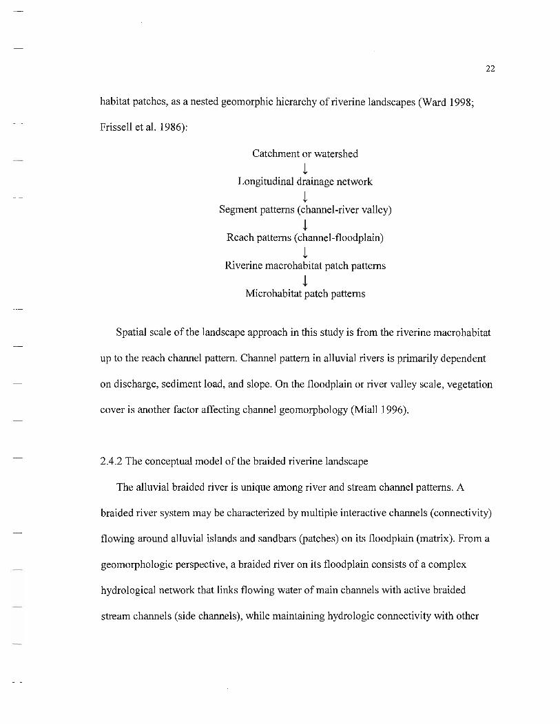
habitat patches, as a nested geomorphic hierarchy of riverine landscapes (Ward 1998;
Frissell et al. 1986):
Catchment or watershed
t Longitudinal drainage network
t Segment patterns (channel-river valley)
t Reach patterns (channel-floodplain)
t Riverine macrohabitat patch patterns
t Microhabitat patch patterns
Spatial scale of the landscape approach in this study is from the riverine macro habitat
up to the reach channel pattern. Channel pattern in alluvial rivers is primarily dependent
on discharge, sediment load, and slope. On the floodplain or river valley scale, vegetation
cover is another factor affecting channel geomorphology (Miall 1996).
2.4.2 The conceptual model of the braided riverine landscape
The alluvial braided river is unique among river and stream channel patterns. A
braided river system may be characterized by multiple interactive channels (connectivity)
flowing around alluvial islands and sandbars (patches) on its floodplain (matrix). From a
geomorphologic perspective, a braided river on its floodplain consists of a complex
hydrological network that links flowing water of main channels with active braided
stream channels (side channels), while maintaining hydrologic connectivity with other

Figure 2-1. Conceptual model of a braided riverine landscape. The question symbols indicate those "hot spots" for studying the hydrological connectivity.
On a geological time scale, these diverse geomorphologic types and their spatial
configurations on the floodplain represent different geological process stages of the
23
braided river, and reflect a series in fluvial geomorphic succession. The general trend of
the fluvial succession, as results from the processes of fluvial erosion and sedimentation,
is: main channel --.active braided channels --. backwater or abandoned braided channel
--. slough or pond. However, natural disturbance such as an extremely high flood-pulse
may rapidly shift the sequence or invert the order.
My study of the river system focused on the ecological time scale and habitat and
landscape spatial scales. During my study period, the relative spatial locations and
geomorphic characteristics of the riverine habitats may be seen in dynamic equilibriums,
and may not change significantly, except those directly connected with the main channels.
24
My study of the river system focused on the ecological time scale and habitat and
landscape spatial scales. During my study period, the relative spatial locations and
geomorphic characteristics of the riverine habitats may be seen in dynamic equilibriums,
and may not change significantly, except those directly connected with the main channels.
Riverine aquatic habitats on the floodplain are diverse and dynamic in their
hydrological conditions: standing or low flowing water may be present perennially or
seasonally; surface water of a riverine habitat mayor may not connect directly to a stream
channel. However, a patch of riverine habitat usually connects with a stream channel
indirectly through shallow groundwater, because it forms on highly permeable sandy to
silty-sandy alluvial sediments adjacent to the stream channel where the shallow
groundwater table is usually very close to the surface (Henszey and Wesche 1993). Thus,
both surface and subsurface hydrologic linkages should be considered when studying a
riverine aquatic patch.
Patch size, or a real horizontal riverine aquatic habitat is study dependent. For the
purposes of this hydrologic linkage study, only the wetted area was considered for area
calculations. The boundaries of a riverine aquatic habitat are determined by edges of the
wetted surface area of the habitat, surface water elevation, and the groundwater table.
Edges and area of the wetted surface water may be identified by direct measurement in
the field and integrating survey information of topography, vegetation and soil types
surrounding the riverine habitat. The groundwater table is assigned as the subsurface
boundary of a riverine aquatic habitat, since it responds to the hydrologic fluctuation of
adjacent stream channel(s) and may be used as a dependent variable of subsurface

hydrologic linkage. The groundwater table also represents the vertical position of the
surface-water/groundwater ecotone, an important component of a river ecosystem.
2.4.3 Hydro-geomorphological approaches to the riverine landscape
25
In this research, I address hydrologic linkage of the riverine landscape by studying the
hydrological connectivity of riverine habitats on the floodplain of the Middle Platte River.
The hydrological connectivity is an essential attribute of the riverine habitats. This may
be studied by: (a) analyzing and mapping the hydrological connections (landscape
structures) between the main channel and associated riverine habitats, and (b) calculating
and evaluating the strength of hydrological interactions (functions) between them.
The structure, or spatial pattern of the hydrologic connectivity is a very important
component of riverine landscape. The hydrological interactions between the riverine
habitats and main channel affect other ecological functions, such as flux of nutrients and
movement of aquatic organisms across the riverine landscape. Therefore, study of the
hydrological connectivity is fundamental to understanding the degree to which the
riverine landscape facilitates or impedes movement among resource patches, i.e., the
landscape connectivity, as defined by Taylor et al. (1993).
To clarify explanation and facilitate the study offield survey, hydraulic monitoring,
and statistical analysis, I introduced the following denotation:
Hr -- Height of water level in a river channel, usually read from a staff gauge;
Hs -- Height of surface water level in a nearby riverine habitat, read from gauges
installed in the studied habitats;

Hg -- Height of water level in a piezometer that was installed in a stream or a
nearby riverine habitat, where the hydraulic head underneath the stream bottom, or
groundwater table beneath the riverine habitat was measured.
26
The fust step of my research project was monitoring how the riverine habitats respond
to discharge fluctuations in main channel(s). Networks of hydrological monitoring wells
and transects were established to measure surface and subsurface water fluctuations in
both the main channels and riverine habitats simultaneously. Figure 2-1 shows a detailed
illustration of such monitoring network. The interactions of the main channel and the
riverine habitats with groundwater may be determined from water table contour maps
(Winter et al. 1998), or by comparing water levels of a piezometer (Hg) with a stream
gauge (Hr) near the piezometer (Hudak 2000).
The second step was sampling surface water, analyzing field physicochemical
conditions, survey topography, land cover and land use, and soil/sediment properties.
The third step was analyzing spatial patterns of the riverine landscape with
geographical information systems (GIS), remote sensing images, and spatial statistical
techniques at different spatial scales. A series of digital map-based spatial explicit models
(SEM) may be generated to locate the habitat patches, superimpose the groundwater table
distribution maps, and incorporate changes of riverine habitats with the given
hydrological regime.
The fourth step was classifying the riverine habitats based on the hydrological and
geomorphological information collected during the first three steps. The grouped riverine
habitat types may be used for assessing their hydrological and ecological functions .

N
W*' S
• Piezometer
6 Stream Gauge
---- Transect
--I.. River Flow Direction
200 o 200 400 Meters --- -
Figure 2-2. Design of hydrologic monitoring network at study area 13. about 4.5 km southeast of Kearney, Nebraska.
tv '-l

28
The fifth step was quantitatively examining hydrological interactions between river
discharge and water levels in the riverine habitats. This is necessary for studying the
spatial diversity of the hydrology and its influence on patterns of biodiversity. Multiple
statistical techniques such as Correlation Examination and Multiple Regression Analysis
(Helsel and Hirsch 1992) were applied to examine the complex hydrologic relationship
between main channels and various riverine habitats.
The sixth step was evaluating effects of natural and human disturbance on the riverine
habitats and uncertainty of the analyses. By comparing results of the statistical models, I
evaluated differences of morphological and ecological characteristics among the diverse
riverine habitats.
2.4.4 Physical principles of the riverine hydrologic processes
Based on the continuity equation of water mass conservation (Chow et al. 1988), the
water budget of a riverine surface water body, with an unsteady, constant density flow at
time t, is derived by considering the mechanisms by which water may flow in (I(t), flow
out (O(t), and be stored in this predefined "wetted" patch area of the riverine habitat (S).
The net flow (total inflow minus total outflow) must be equal to the change in surface
water stored in the patch area of the riverine habitat (dS) over a time interval (dt):
dSldt = I(t) - O(t) (2-2a)
I(t) and O(t) are flow rates, having dimensions [L3r 1], while S is a volume, having
dimension [L3], and t is time, with dimension [T].

29
The following factors of water balance in a riverine aquatic system need to be
considered as major components in a conceptual model for studying hydrologic linkages
of a riverine habitat with an adjacent river channel: precipitation (P), surface inflow (Qs),
recharge to river from river bank (Qb), evaporation (E), transpiration (T), surface outflow
(Qo), and discharge to river bank (Rr). Thus, continuity Equation 2-1a can be expressed as
dSldt = (P + Qs + Qb) - (E + T + Qo + Rr). (2-2b)
In practice, "the evaporation and transpiration are often combined as evapotranspiration
(ET) since it is both difficult and unnecessary to separate these two processes" (Stephens
1996). Thus, one may write Equation 2-1 b as
dSldt = (P - ET) + (Qs - Qo) + (Qb - Rr) (2-2c)
All variables on the right-hand size of the equations have units of [L3r l]. Dividing both
sides ofthe above equations by the area of riverine habitat patch (A), the water budget
components can be expressed with dimensions [Lrl] (Stephens 1996).
Most hydrologic data are available only at discrete time intervals. On a discrete time
basis with an interval oftime length M, indexed by j, the Equation 2-1a can be rewritten
as
dS = I(t) dt - O(t) dt (2-3)
and integrated over the jth time interval to output
1· l :J ojt:J dS= /ltt- tt
Sj - 1 £-1)61 ()d t-1)t:J Q( }1 (2-4a)
or
j= 1,2, 3, ... (2-4b)
30
where l.J and Qj are volumes of inflow and outflow in the /h time interval with dimensions
[L3], or volumes of inflow and outflow for a unit patch area (in plane view) with
dimensions [L]. Denoting the incremental change in water storage over time interval M as
(2-5)
Suppose that the initial storage in a riverine water body at time t = 0 is So, then,
j
Sj = So + I (i; - Q) (2-6) i= l
which is the discrete-time continuity equation, described by Chow et al. (1988). Thus, the
discrete-time continuity equation for a water body of the riverine aquatic habitat can be
written as:
j
Sj = So + L [(~ + Qs,i + Qb,i )- (E1'; + Qo,i + Rr,i )] (2-7) i=l
having dimensions [L3] or [L].
The right-hand side of Equation 2-lc and Equation 2-6 represents three major water
exchange processes occurring in a riverine aquatic patch: vertical water exchange
between the atmosphere and surface water, horizontal surface water exchange, and
shallow groundwater exchange. For the purposes of this study, the vertical water
exchange between the atmosphere and surface water may be quantified by using available
data of precipitation and evapotranspiration from local weather stations. The horizontal
surface water exchange may be considered when a channel connection with the patch
exists, and Qs equals zero if there is no surface connection between the patch of water

31
body and a stream channel or any other nearby surface water body. The portion of
shallow groundwater exchange underneath the riverine habitat, (Qb - Rr) , should include:
(a) riverbank storage to the riverine water body; (b) river recharge from the surface water
body (i.e. seepage of water from and into the stream bank), (c) soil-water stored in the
unsaturated subsurface ofthe riverine area when there is no surface water in riverine
habitats (this often occurs in a dry summer event), and (d) shallow groundwater moving
in the saturated alluvium beneath the riverbed and the riverine aquatic habitat.
2.4.5 Research assumptions
The following assumptions and discussions consider a patch of riverine habitat as a
spatial scale, and a unit of day for the temporal scale.
First, it was assumed that surface water appears only when the lower unsaturated layer
becomes saturated. Therefore, any surface water input to a riverine habitat patch (rainfall,
or stream flow, etc.) is either channeled or ponded. This assumption is based on the fact
that (a) the groundwater table in a riverine zone is very shallow, usually less than 2 m
below surface; (b) surface water accumulated on the floodplain of the river by a rapid
rainfall event either quickly infiltrates into the shallow saturated groundwater layer, or is
removed into stream channels by horizontal runoff 01 oinov et al. 1999); and (c) riverine
habitats adjacent to a river channel are mostly on porous media such as coarse sand, sand,
and silty-sandy alluvium. These sediments have a relatively higher hydraulic
conductivity (K = 10-1-1 02m/d) (Freeze and Cherry 1979; Heath 1983; Stephens 1996);

infiltration rates vary with similar magnitudes as that of the hydrologic conductivity
(O.048-21m1d) (Skaggs and Khaleel1982).
32
With this assumption, infiltration processes and unsaturated subsurface flow are not
considered separately from saturated groundwater processes, because the water level data
used in this study were collected during relative longer periods of time (2-3 day interval
in summer, and 7 day in spring and fall).
Second, sections of the saturated layer beneath channeled and ponded surface water
bodies are assumed to be connected hydrologically, more or less, depending on their
relative distances and the properties of the riverine alluvium media (such as a fine sand
sediment clogging the bottom of a riverine water body). This is the precondition of
correlation and regression analyses. The assumption is reasonable for this study because
of the general permeable properties of the fluvial sediment. Although silty and loamy
soils or a sandy sediment layer are predominant in most of the riverine habitats, there was
no clay layer found underneath any of the studied sites, nor was there a concrete structure,
such as ditch, canal, or levee in the study areas.
Third, it was further assumed that any loss of surface water or output from the stream
channels and riverine habitat patches would lead to replenishing or discharging of water
from the underlying saturated layer, and from another surface water body if there is any
surface hydrologic connection between them.
Fourth, it was also assumed that within the same travel distance of water flow, the
horizontal flow rate of groundwater in the saturated layer is slower than that of surface
water movement through stream channels, if a surface hydrological connection existed.

33
This is based on Darcy's Law and characteristics of a porous alluvium. When the surface
hydrological connection is "cut-off' (i.e. the flow rate of surface water equals zero),
however, the contribution of groundwater becomes significant.
Assumptions regarding the floodplain alluvial sediments as are to follow: (a) the main
channel and riverine stream channels over the study areas are shallow, only partially
penetrating the alluvial aquifer; (b) the thickness of the floodplain alluvial aquifer is
significant comparing with the channel penetration, and relatively constant along the
riverine areas, based on reports from previous hydrogeological investigations (Bentall
1975); (c) there is no low hydraulic conductivity streambed clogging of the main channel
according to the in-channel hydraulic conductivity measurement results of Landon et al.
(200 1) and visual inspections of streambed sediment profiles in the studied reaches; and
(d) the aquifer hydraulic heterogeneity at the reach and riverine landscape scales may be
represented by relatively discrete spatial domains or patches, in which, relatively
homogeneous hydraulic properties may be observed. The boundaries of the domains may
be distinguished by discontinuities in the riverine habitat characteristics from their
surroundings. Soil survey maps and my in-field soil/sediment inspection results helped
the estimation of the aquifer hydraulic heterogeneity.

34
Chapter 3. Methodology
3.1 Study areas
The riverine aquatic habitat addressed here refers to a patch of water body existing
on the alluvial floodplain of a river that fish, wildlife, or other organisms use as their
habitat. Fieldwork for this study was conducted from summer 1996 to fall 1998. A total
of 50 sites in 15 study areas were selected along the reach of the Middle Platte River
between the Highway 281 (Exit 312 of 1-80) at Grand Island and three kilometers east
of the Exit 248 ofI-80 at Overton (Figure 3-1). The studied habitats covered about 26
km (16 miles) of river segments along this 109 km (68 miles) reach between Overton
and Grand Island.
The study sites were located in 42 individual stream channels, backwaters, ponds
and wet meadow sloughs. The width, depth, and wetted perimeter of the studied water
bodies were surveyed along each transect. Black/white and color-infra-red (CIR) digital
orthophoto (quarter) quadrangles (DOQ) (NDNR 1999; USGS 2000b) were used for
mapping the study areas and identifying land cover and surface hydrological
connectivity. Land cover and other landscape characteristics of major aquatic habitat
types in the Middle Platte River floodplain are summarized in Table 3-1 , based on
analysis results and field surveys of this study. Figure 3-2 shows an example ofland
cover image map at study area 13, about 4.5 km southeast of Kearney, Nebraska.
In general, the Middle Platte River has one or two broad, braiding main channels in
upstream of Kearney, Nebraska, and multiple main channels downstream from
Kearney. The main channels link numerous braided side-channels on the

Legend
• Study Area
V USGS Gauging Station
o Weather Station
Scale IOkm 10 20km
Source of the base map: The Platte River Program, USGS (USGS, 2000b)
List of the Study Areas
1. Mormon Island 2. Wolback 3. Crane Meadows 4. Brown Tract 5. Caveney Tract 6. Wood River Sand Pits 7. Dahms Tract 8. Uridil
9. Martin' s Ranch 10. Dipple II. West Rowe Sanctuary 12. Speidel! Tract 13. Wyoming's Property 14. The John's Property 15. Cottonwood Ranch
Figure 3-1. Location of the study areas, USGS' stream gauging stations, and weather stations along the Middle Platte River. w Vl

Table 3-1 . Characteristics of major aquatic habitat types in the Middle Platte River floodplain, summarized based on analysis results and field surveys ofthis study.
Habitat type Main Channel Side-channel Backwater Wet Meadow Slough Pond
Most time lotic; woodland Most time lentic;
Aquatic condition Lotic; open space; riparian belts
surrounding with riparian Most time lentic Stagnant and hydrophytes
Upstream channel flow; Main channel ; Side-channel or main
Groundwater; precipitation; Groundwater; overbank Main source of inflow groundwater; overbank channel; groundwater;
Rainfall flow overbank flow
overbank flow flow; rainfall
Downstream channel flow; Downstream channel; Downstream channel; wet Downstream backwater; rnflltration, and overflow
Main source of outflow discharging to side-channel and backwater
backwater; wet meadow meadow; Side-channel; pond when flooding
Water dynamic Fast flow Medium-slow flow Slow flow; sometime
Very slow or stilling Standing water stilling in summer
Current velocity (cmls) > 30 15-30 10 - IS < 10 0
Water depth (cm) 30 - 120 20 - 50 5 - 40 5 - 20 > 50
Substratum Coarse sand and gravel Sand and gravel Fine gravel, sand and silt Sandy silt and clay loam Clay loam, silt or sand
Wide open braided Opened or riparian channel Small channel or pond with Flat wet meadow or
Geomorphology channels with sandbars with pool-riffle sequence riparian belts
elevated sand ridges with Varied lowland or oxbow swales
Dominant plant Sandbar willows Willows and cottonwood
Bulrush, cattail, dogwood, Sedges, giant reed, buried, Bulrush, cattail, sedges
communities willow shrubs; bulrush, cattail
Wider corridor with Small linear patch Long linear patch in wet Small patch mosaic in wet
Landscape geometry patches of sandbars; Narrow corridor connected or near river meadow matrix meadow or backwater
braided network channel
Land use Water transportation; Channel network; irrigation Grazing; hunting; Grazing; haying; wildlife
Grazing; fishing; hunting crane's habitat; recreation runoff; grazing; hunting recreation conservation; hunting
W 0'\

37
floodplain. In some places, there are multiple braided branches of main channels in the
wide riverbed where the stream flow is shallow. The main channel is a broad but shallow
(range from 0.5-1.5 m), sand bedded channel during high discharge periods. It becomes
braided at low stages of discharge when the tops of in-channel sandbars were exposed.
The inner characteristics of the main channels were not the focus of this study.
Distinctions between a side-channel and a main channel are the degree of difference
in their geomorphological features (such as length, width, and shape) and their
hydrological characteristics (such as flow depth, velocity, and hydraulic linkage). A
typical side-channel is a reach of braided stream fully connected with a main channel of
the river. It is usually several hundred meters long, less than 15 m wide, with shallow
water and a lower flow rate than the main channel. It is a lotic habitat at most times of a
year. Water velocity in a side-channel is usually 0.15-0.30 mls. During the low flow
season, side-channels may be embedded in a wide main channel, as so called "secondary
channels" (Petts and Amoros 1996).
Backwaters usually connect with main channels and active braided channels. A
backwater does not change in size, depth or flow velocity as much as a side-channel.
Thus, a backwater habitat has relatively stable hydrophyte communities and higher
percent cover of vegetation than in a side-channel. A backwater habitat is also more
lentic than a side-channel. During most of the year, the velocity of backwater flow is
usually less than 0.15 mls. The length of backwater bodies varies from less than 100
meter to several hundred meters.

N
W* E • MaIn Channel
i Side Channel
i Backwater
® Riparian
Shrubs or Sandbar
0 Cropland
Pasture
Figure 3-2. Land cover of a reach of Middle Platte River floodplain, about 4.5 km southeast of Kearney, Nebraska
Sloughs are linear shape, shallow water bodies in wet meadows and in transitional
zones of wet meadow and riparian habitats. Sloughs are usually located relatively far
from a main channel, and hydrologically in semi-Ientic and lentic status. Sloughs are
formed geomorphologically in former side-channels during evolution of the floodplain.
38
Woody vegetation presents along the sloughs, except those managed wet meadow areas.
There are also non-linear shape, isolated, small shallow water habitats in wet
meadows and riparian woodlands, which are normally called ponds. A pond, as defined
by Franti et al. (1998) is:

"a small body of standing fresh water, either natural or artificial,
usually with negligible current and having more or less continuous
vegetation from the marginal land into the water" (Franti et al. 1998).
39
Pond depth varies from less than 1 meter (shallow lowland ponds) to several meter
(deep gravel pits). Some shallow ponds (with mean depth less than 2 m, and hydric soils
and hydrophytic vegetation along edges) qualified as wetlands by definition (Mitsch and
Gosselink 2000); while many deeper ponds have abrupt edges, and lack hydric soils and
hydrophytic vegetation.
3.2 Data sets
3.2.1 Hydrological data
Hydrological parameters measured were: stream water stage and water current
velocity in the river channel (either main channel or side-channel) adjacent to a study
site; surface water stage, depth and current velocity in riverine aquatic habitats; and
groundwater table measured with a mini-piezometer at the same point where surface
water level was measured in an aquatic habitat.
River discharge data were collected from three USGS gauging stations at Overton,
Kearney, and Grand Island. Daily river discharge and long-term peak flow data were
downloaded from the USGS' on-line stream flow data service (USGS 2000a). Data of
monthly and annual discharges at the USGS' Kearney, and Grand Island stations were
collected from USGS publications (Boohar et al. 1996,1997, 1998; Boohar 1999, 2000).

40
3.2.2 Weather and climate data
Weather and climate data used in this study were provided by the High Plains
Regional Climate Center, University of Nebraska-Lincoln. The data were collected from
five weather stations located within 3 to 16 km (2-10 mi.) of each study area, namely
Overton, Kearney, Shelton, Wood River, and Grand Island (Figure1). Data used included
daily average air temperature (T, °C), total daily precipitation (P, mm), and daily
potential evapotranspiration (ET, mm). The potential ET values were calculated from the
Penman combination equation (Rosenberg et al. 1983) with a Nebraska wind function
(Hubbard 1992; Robinson and Hubbard 1990). The climate data from 1996 to 1998
indicated a close to "normal" condition of mean monthly temperature during the study
period, with some deviation from normal in the amount of rainfall received by the study
region (HPRCC-UNL 2000; National Weather Center, USA, 1999).
3.2.3 Soil/sediment and land cover data
Soil/sediment characteristics were taken from publications of the U.S. Department of
Agriculture, Soil Conservation Service (USDA-SCS 1962, 1973, 1974, 1984), and
augmented by observations of soil profiles taken on-site and soil texture analyses for
some study sites. Streambed sediment profile visual inspections (Morris and Johnson
1967) were conducted in the studied reaches.
Land cover of riverine habitats was surveyed on-site in May and August 1998.
Species composition, richness, average height, and cover areas were measured and
compared over the growing season. Distribution of the vegetation was identified based on

41
the Normalized Difference Vegetation Index (NDVI) using spatial analysis technique in
ArcView GIS (ESRI, Inc. 1999). Results of the soil and vegetation surveys were used for
land cover types and landscape pattern analyses. Previous vegetation and land cover
studied results (Currier 1982,1995,1999; Currier et al. 1985; O'Brien and Currier 1987)
were considered in the surveys. Landscape features of the studied aquatic habitats were
summarized in Table 3-1.
3.2.4 Surface water physicochemical data
Surface water samples were collected for chemical analysis bimonthly during the
growing seasons (Table 3-2). Physicochemical parameters measured in field were: water
temperature, pH, dissolved oxygen, conductivity, and salinity. Analyzed chemical
parameters include: (a) dissolved nutrients: Nitrogen (N03--N, N02--N, and NH/-N) and
Phosphate (P04-3-P); (b) major dissolved ions: Calcium (Ca2l, Magnesium (Mg2l,
Potassium (Kl, Sodium (Nal, Sulfate (SO/-), and Chloride (CI l); (c) dissolved trace
elements: Aluminum (AI), Arsenic (As), Bismuth (Bi), Boron (B), Cadmium (Cd),
Chromium (Cr), Cobalt (Co), Copper (Cu), Iron (Fe), Lead (Pb), Manganese (Mn),
Molybdenum (Mo), Nickel (Ni), Titanium (Ti), Vanadium (V), and Zinc (Zn).

Table 3-2. Water sampling periods and corresponding main channel flow conditions.
Sampling Period Group ID S~asQnanlydrological Condition Range of Discharge in Main channel
May 23-27, 1996 9605 Spring, normal water level 42.46-70.79 m3 Is (1,500 - 2,500 cfs)
Aug. 06-09, 1996 9608 Summer, normal water level 56.63-70.79 m3/s (2,000 - 2,500 cfs)
Apr. 17-20,1997 9704 Spring, normal water level 48 .14-73.62 m3/s (1,700 - 2,600 cfs)
Jun. 14-17, 1997 9706 Summer, high water level 99.11-212.38 m3/s (3,500 - 7,500 cfs)
Aug. 14-20, 1997 9708 Summer, high water level 82.12-121.8 m3/s (2,900 - 4,300 cfs)
Oct. 19-22, 1997 9710 Autumn, normal water level 3 59.46-82.12 m Is (2,lOO - 2,900 cfs)
Jun. 9-12, 1998 9806 Summer, normal water level 67.96-82.12 m3/s (2,400 - 2,900 cfs)
Oct. 31-Nov.19, 1998 98lO Autumn, normal water level 56.63-70.79 m3/s (2,000 - 2,500 cfs)
+>tv

43
3.2.5 Spatial imagery data
Several sources of imagery data were utilized in this study.
(1) Digital orthophoto quadrangle (DOQ) images of the study region, products of the
National Aerial Photography Program. Two types of these computer-compatible
representations of aerial photographs were used as base-map layers for creating and
referencing other geo-spatial data in the study region: (a) black-and-white color images
acquired for the summers of 1993, mapped to 1: 12,000 scale accuracy specifications
(NDNR 1999); and (b) color infra-red images acquired for the summers of 1998 at scale
of 1 :40,000 (USGS 2000b). The images were digitized and geo-referenced with I-meter
ground resolution and stored in 256 gray levels of spectrum and projected in the
Universal Transverse Mercator (UTM) coordinates based on the North American Datum
of 1983 (NAD 83) (NDNR 1999; USBR 1999).
(2) One infrared aerial photo (achieved in 1995), provided by U.S. Fish and Wildlife
Service at Grand Island, Nebraska, was scanned as a TIFF-formatted image file. It covers
one of the study sites near Kearney, Nebraska. The scanned image was then rectified with
reference to the DOQ images using the Polynomial Geometric Model of Raster Image
Rectification in the ERDAS IMAGINE 8.4 (ERDAS Inc., 1999).
(3) Three series of true color aerial photos (acquired for summer 1996, 1997, and
1998) purchased from the Farm Service Administration (USDA) in Buffalo County,
Dawson County, and Hall County, Nebraska were also used as reference images to
compare and identify changes of riverine aquatic habitats in the study areas.

44
3.3 Methods
3.3.1 Hydro-geomorphological classification of the aquatic habitats
The aquatic habitats in the Middle Platte River floodplain were classified by
integrating their environmental features (Table 3-1) characterized according to my
landscape survey and hydrological monitoring data from the 50 study sites located in 42
riverine habitats and main channel reaches in15 study areas (Figure 3-1). The habitat
classification is based on the fluvial geomorphological features (shape, width, depth, and
surface connection with the main channel, etc.), surface water hydrologic dynamics (lotic
or lentic, permanent or intermittent), and land covers (riparian, wet meadow).
Hydrographs and scatter plots of the main channel discharge-habitat water level for each
of the study sites were compared to analyze discharge changes and variations of water
levels in the main channel, surface water levels, and groundwater tables in each
associated riverine water body. The classification system is shown in Table 3-3.
Comparing with Table 3-1, several subtypes of riverine habitats were identified in this
study as discussed below:

Table 3-3. Hydro-geomorphological classification system of aquatic habitats used in this study.
* Habitat Class Level Criteria of Classification
Habitat Habitat Surface
Type Subtype Fluvial Geomorphology Surface Water Connection Water Land Cover
Dynamics Main Sandbar;
Wide and braided, open, linear, Lotic, Water and large channel braided Link with SC, TB, and BW (MC) stream
with large sandbars permanent sandbar and islands
Side-channel Medium width, linear, semi-open Fully-connected to MC
Lotic, Small sandbars Side-channel (SC) or canopied, shallow water permanent and riparian
(SC) Tributary Medium width, linear, semi-open Partially-connected to MC; Lotic, Riparian, rangeland
(TB) or canopied, shallow water surface inflow from upland permanent Connected
Very shallow, hydrophyte present; Partially-connected to MC Semi-Iotic; Small sandbars Backwater
Backwater (CB) medium width, linear, Most canopied in most of a year permanent and riparian
(BW) Disconnected Very shallow, hydrophyte present; Disconnect from
Semi -lentic; Backwater
Medium width, linear, Most canopied MC in most of a year permanent or Riparian
(DB) intermittent Permanent
Very shallow, hydrophyte present; Disconnect from MC; Semi-Iotic;
Wet meadow; Slough
narrow width, linear, Most canopied some link to BW or SC permanent
riparian Slough (PS)
(SL) Intermittent Very shallow, hydrophyte present;
Disconnect from MC; Semi-Ientic; Wet meadow;
Slough narrow width, linear, Most canopied
some link to BW or SC intermittent (IS)
Riparian Pond Non-linear, canopied, No direct surface water Lentic; most Riparian
(RP) hydrophyte present or absent; connection with other habitats permanent Pond
Wet Meadow No direct surface water Lentic; (PN)
Pond Non-linear, non-canopied,
connection with other habitats intermittent or Wet meadow (WP)
hydrophyte present or absent; permanent_
------ - -
* Criteria of classification refer to that presents in "normal" conditions (i.e. excluding flood and extremely drought periods), as quantitatively defined as: (1) Average channel bankfill/water width (m): wide (> 50/35), medium (15110 - 50/35), narrow « 15110); (2) Surface water depth (m): shallow (0.3-0.5), very shallow « 0.3); Canopy cover area (%): canopied (60-80), semi-open (20-59), open «20); (3) Hydrophyte present: > 10% of surface area; (4) Surface water connection: fully-connected: connected at both upstream and downstream ends; partially connected: either upstream or downstream end.
+>VI


46
Some tributaries of the Middle Platte River are termed "side-channels" in general, but
they are much longer, paralleling a main channel for several kilometers before they
merge with the main channel. Tributary streams usually connect with a side-channel or
directly flow into the main channels. They may also link with sand and gravel pits,
irrigation canals, ditches, or small tributaries from uplands, and receive water from
upland runoff, groundwater recharge, irrigation return flow, and overbank flow from
main channels when they are flooded. These longer side-streams appear to belong to side
channels morphologically; however, they have different hydrological patterns. Thus, I
sub-classified them as "tributary", a subtype under the category of side-channel for this
study.
A backwater represents a habitat intermediate between lentic and lotic systems. Flood
scouring and alluvial aggradation are two fluvial geomorphologic processes that alter the
morphology of backwater habitats and their hydrological connectivity with the main
channels. The backwater habitats are divided into two subtypes based on their surface
hydrological connections with the main channels. Hydrological characteristics of
backwater habitats in the braided river system depend upon their locations in the
floodplain and the habitat geomorphologic features.
It needs to mention that the connected backwater subtype includes backwaters located
within the broad main channels and those in braided channels adjacent to the main
channels. The backwater habitats located inside the broad and braided main channel may
be called as "instream backwater", or "intermittent backwater" because they appear

47
during low-river-flow seasons, and are submerged during high flow seasons. Thus, the
instream backwater habitats are highly dynamic and unstable. Peters et al. (1989)
described distribution of the instream backwater in the Lower Platte River as a water
body located either at the downstream end of a large sandbar in a broad channel, or
presents at the interface of a main stream channel, i.e. an area between a large sandbar
and the adjacent riverbank (Peters et al. 1989). These distribution patterns are similar in
the main channels of the Middle Platte River.
Other connected backwater habitats are found in some inactive channels, or small
stream braids adjacent to a main channel. From a geomorphological point of view, those
inactive channels appear to be former side-channels. These backwater bodies are
disconnected from the stream channel at their upstream entries, and are connected to
active stream channels, either main channels or side-channels, at their outlets; thus, the
backwater channels are fed by subsurface -shallow groundwater or bank seepage from the
main channels during normal stream flows. Surface backflow from main streams input
the backwater habitat through their downstream outlets during high stream flows, and
overbank flow when flooding. During high flow periods, part or entire areas of backwater
channels may be submerged, and backwater channels may become active streams.
Unlike the connected backwaters mentioned above, the disconnected backwater is a
type of "isolated backwater" in a "cut-off channel" (Bornette et. al.1998) or a so-called
"abandoned-channel" (Nanson and Croke 1992, Carson 1984). This refers to backwater
areas that have been partially or fully separated from the main stream at both ends of their
channel, or have been disconnected from stream channels by bank stabilization or beaver

dams. Compared with the first kind of backwater bodies, this type of backwaters is a
lentic aquatic environment with relatively stable surface water levels. It is fed by bank
seepage, overbank flow, and groundwater discharge. There is no surface water
connection with the main channel for this type of backwater habitat.
48
Slough habitat type is subdivided into two subtypes: permanent slough and
intermittent slough. Wet meadow sloughs have more lentic hydrological characteristics
than backwaters. In contrast to a backwater body, it does not directly connect to a main
stream via surface flow. Instead, a wet meadow slough usually links to a side-channel or
a backwater body. On the floodplains of the Middle Platte River, wet meadow sloughs
may be separated from main stream channels by natural sand levees or other
aggradational alluvium or debris deposits (Petts and Amoros 1996), beaver dams, or man
made constructions for irrigation, drainage, bank stabilization, highways, recreation, etc.
A pond is a small, non-linear patch of standing water in riparian or wet meadow that
is surficially isolated, and distant from any stream. Stewart and Kantrud (1971) classified
natural ponds and lakes in the glaciated prairie region as ephemeral, temporary, seasonal,
semi-permanent, permanent, etc. According to this classification, most of the riverine
ponds in the Middle Platte River floodplain are semi-permanent or permanent ponds. For
purposes ofthis study, ponds were classified into two sub-types according to their land
cover composition and geomorphologic location: "riparian ponds" in riparian woodland
habitats, and "wet meadow ponds" in wet meadow habitats. In general, grain sizes of the
wet meadow ponds subsurface sediments are smaller than that of riparian ponds, although
it can been seen in both of the subtypes that there is a very thin silt or clay-sand layer
covering the bottom.
3.3.2 Correlation analysis on the main channel-riverine habitat interactions
49
Correlation analysis was conducted to identify strength ofthe hydrological
interactions between discharge, precipitation, temperature, evapotranspiration and water
level changes in different types of the riverine habitats. The Kendall's Tau (1')
measurement was used for the evaluation of correlation of the paired monitoring data.
The 1'measures the strength of all monotonic (linear and nonlinear) relationships between
x and y, and is based on ranks, so the procedure is resistant to the effects of outliers
(Helsel and Hirsch 1992). "The l' coefficients are based on the number of concordant and
discordant pairs. A pair of rows for two variables is concordant if they agree in which is
greater. Otherwise they are discordant, or tied" (SAS Institute Inc. 1995).
The time delay of riverine habitat water levels in response to the river stages adjacent
to the habitats was less than an hour for those riverine habitats connected with the main
channel, and within several hours for those disconnected riverine habitats according to
my field water level measuring results and previous reports (Henszey and Wesche 1993;
Hurr 1983; Lugn and Wenzel 1938; Wesche et al. 1994). The correlation ofthe paired
water levels between the main channel and the adjacent habitats was examined based on
the monitoring data collected at time-intervals of2-3 day in summer and 7 day in spring
and fall seasons. Since the Kendall's 1'coefficient correlation is calculated based only on
the number of concordant and discordant pairs, the effect of the time delay of the water

level response on the correlation analysis is not significant, and it was treated as an
random error in the statistic analyses.
50
The time delay of wet meadow slough habitat water levels in response to precipitation
is similar as that to the main channel water stages. Based on continual groundwater
monitoring data collected from water level recorders at three observation sites in wet
meadow along the Middle Platte River (Henszey, unpublished data, 1995-1998), a local
rainfall event and associated surface runoff in sloughs may cause a maximum rise in the
groundwater table within an hour or so. But it often takes 5-7 days for the elevated water
table to reach a new equilibrium with the river stage and evapotranspiration (Henzey
2000). Hurr (1983) also indicated the similar pattern of the time delay for the water levels
in the wet meadow habitat. Because we usually measured the water level and
groundwater table changes 12-24 hours after a rainfall event, the time delay of the water
level in response to precipitation was also considered as "noise" during the water level
fluctuation at the multi-day time scale used in this study.
At each of the study sites, the following paired or grouped river stage data and habitat
surface water level and groundwater table data were used for the correlation analysis:
Riverine Habitat Surface Water Level vs. River Stage Level (Hs vs. Hr);
Riverine Habitat Groundwater Table vs. River Stage Level (Hg vs. Hr); and,
Riverine Habitat Surface Water Level vs. Groundwater Table (Hs vs. Hg).
The riverine habitat water level and groundwater table data were also correlated to the
river discharges reported from the closest USGS' gauging station to check riverine
habitats in response to the instream flow change (Hs vs. Q and Hg vs. Q) at the landscape

51
scale. The average travel time of the river flow in the main channel was estimated about
80 km/day (50 mi/day) based on the discharge data collected from three gauging stations
(USGS 2000a). Most of my study sites were located within 30 km from the closest the
gauging station (Figure 3-1). Thus, the daily average discharge was used for the statistic
analyses in this study to reduce the time delay effect between the study sites and the
closed gauging stations.
3.3.3 Cluster analysis on spatial pattern of the riverine habitat types
Cluster analysis of characteristic hydrological data was undertaken to develop
groupings based on the degree of similarity (Johnson and Gage 1997). I used T
correlation coefficient as a parameter for clustering pairs of hydrologic linkages at the
study sites. Classified data groups were used to examine the spatial patterns of riverine
habitats and their hydrological connectivity with the main channels according to their
spatial distributions. To incorporate both the channel width (w) and the distance between
the main channel bank and a riverine habitat (d) in analysis, a location parameter (Lr) for
the riverine habitats was introduced as:
Lr = (d + w/2)/w (dimensionless) (3.1)
i.e., a ratio of the distance between the center ofthe main channel and a riverine habitat to
the main channel width.
52
3.3.4 Regression analyses ofthe main channel discharges-riverine water levels
Regression analysis and curve fitting techniques were applied to the data from
riverine habitat water levels (as response variables), and main channel discharges and
local area climatic data (as explanatory variables) to estimate or predict the hydrological
changes between the main channels (represented by daily mean discharges) and the
various riverine habitats (represented by their surface water and groundwater levels). The
general form of the multiple linear regression (Helsel and Hirsch, 1992) for modeling of
the stream-riverine habitat interaction is denoted as:
(3.2)
where y is the response variable, such as surface water level (Hs, m) or groundwater table
(Hg, m) of the riverine habitat; bo is the intercept; b l , b2 , ... , bk are a set of coefficients
for the explanatory variables: XI, X2, ... Xk; Xk is an explanatory variable. It may be the
discharge (Q, m3/s), temperatures (T, °C), precipitation (P, mm), and/or
evapotranspiration (ET, mm). 8 is the error and represents the remaining unexplained
variability in the data. Observed significance probability was set as 0.05 for all regression
analyses. Analyses were conducted by: (1) Bivariate regression models of riverine habitat
water levels (Hs and Hg) by main channel discharges (Q); (2) Stepwise multivariate
regression models of riverine habitat water levels using main channel discharges (Q) and
climate data, including temperatures (T), precipitation (P), and potential
evapotranspiration (ET).
53
I also transformed the T, P, and ET data to moving average values at intervals of
three, four, and seven days, using a moving average method introduced by Gomez and
Gomez (1984, pp. 480-483), and Hoshmand (1998, pp. 366-368), in order to match the
temporal scales of hydrological observation to eliminate daily weather variation from the
time series. These transformed variables are denoted as T3, P3, ET3, T4, P4, ET4, T7, P7,
and ET7, respectively. They are correlated with the original T, P, and ET data. Thus, as
candidates for the stepwise regression analysis, they cannot be added simultaneously into
the process of modeling; instead, a combination of discharge with one of the grouped
three-day, four-day, or seven-day variables was used each time. The candidates for
explanatory variables for the regression modeling were first examined for their
correlation, and their significance on the hydrological interaction ofthe stream-riverine
habitats. For example, the temperature and the potential ET variables were correlated.
Thus, they were used separately with other independent variables for the stepwise
regression. The moving average method was also applied to the discharge data, but the
regression outcomes using this type of transformation showed no improvement in the
models.
Three types of residuals plots from each of the regression models were produced and
examined for adherence to the assumptions of the regression models (Helsel and Hirsch
1992), including: residuals vs. predicted values, residuals vs. time, and residuals vs.
normality of residuals displayed by normal probability plot, histogram, boxplot, etc.

54
3.3.5 Analysis of variances on heterogeneity of physicochemical data
For analyses of the physicochemical data, temporal changes were incorporated into
the statistical analyses and discussion as: (a) the entire study period, and (b) eight levels
of the sample seasons. The sample seasons were grouped and notated as the month and
the year when the samples were collected, as described in Table 2.
Normality distribution tests and homogeneity of variance tests (SAS Institute Inc.
1995) were first performed to detect whether the data violated any assumptions of further
statistical analysis. Analysis of Variance (ANOVA) was conducted to test if the level
means of season or habitat were all equal. For those data sets with non-normal
distributions, several nonparametric statistics methods were applied. When the
homogeneity of variance assumption required by ANOVA was found to be violated,
Welch's ANOVA (SAS Institute Inc. 1995) was conducted. Other multiple comparison
techniques, such as Multiple Comparisons for All pairs (MCA), Multiple Comparisons
with the Best (MCB), and Multiple Comparisons with Control (MCC) (SAS Institute Inc.
1995) were also applied to the data analyses. Other influences such as land-use and cover,
and management processes were also considered in interpreting the chemical analysis
data. Boxplots and bar charts were used to illustrate the statistical results and compare the
differences in parameters due to both seasonal change and spatial heterogeneity described
by the habitat category.

55
3.3.6 Spatially explicit models of the riverine landscape
The spatially explicit model (SEM) developed in this study is a GIS-based, digitized
map of actual or simulated phenomena superimposed on a landscape (Withers and
Meentemeyer 1999). The SEMs are used to transform raw photographic image data into
land cover and riverine habitat maps, and visually identify the channel connectivity and
interpret landscape features. Distribution and change of habitat patches and the effect of
other landscape features on the dynamics of the habitats may be studied with such
digitized maps.
A case study site was selected in a wildlife management area of the Middle Platte
River near Kearney. I achieved two "simultaneous" remote sensing images within my
study period to match a recommended flow rate (USGS 2000b; U.S. FWS 1994). Spatial
analysis and geo-statistical modeling processes supported by ArcView GIS (v. 3.2a) were
used to develop a series of spatially explicit, map-based surface water distribution models
based on my field topography survey and hydrological monitoring data. By coupling
groundwater table distribution in the riverine habitats with the land cover spatial data on
the study sites, I analyzed the spatial patterns of the riverine landscape (McGarigal and
Mars. 1995) for this targeted riverine conservation site managed by the U.S. Fish and
Wildlife Service.
The methods used in this research were expected to identify:
(a) The surface hydrological connections between the braided main channel and its
associated riverine habitats in landscape scale by conducting on-site geomorphological

survey, soil and sediment grain sizes analyses, and interpreting braided stream network
with high-resolution digital images;
56
(b) The riverine habitat spatial patterns and configurations by extracting landscape
indices from a suite of riverine landscape theme maps generated from GIS-based spatially
explicit models;
( c) The physical processes influencing hydrological interaction between the main
channel and its associated riverine habitats by developing a series of regression-based
models to examine the hydrological and climatic factors influencing hydrological
interaction between the main channel and the riverine habitats at the habitat scale; and,
(d) The diversity of the riverine habitats by analyzing and comparing the hydrological
connections, the strength of hydrological interactions with the main channels, the
physicochemical data at habitat and landscape scales and at the bimonthly seasonal scale,
and integrating information of environmental components within the riverine landscape.

57
Chapter 4. Results and Discussions (I): Hydrological Connectivity
4.1 Surface hydrological connection and classification of the aquatic habitats
Aquatic habitats in the study areas are quite diverse. Table 3-1 summarizes some of
the significant differences between these commonly recognized habitat types based on
image interpretation and a literature review. According to the detailed information gained
from my on-site fluvial geomorphological surveys, I further classified the riverine
habitats according to quantitative classification criteria on the dynamics of the habitat
hydrology, land cover, and the surface hydrological linkage between the main channel
and the riverine habitats. The criteria and results of the classification system are listed in
Table 3-3 and Figure 4-1. The aquatic habitat type class was organized in two levels. The
first level, habitat type, was classified by the degree of hydrological linkage with the
main channel and morphology of the habitats. The second level, habitat subtype, was
identified based on their hydro graphs and land covers. There are nine habitat subtypes:
main channel (MC), side-channel (SC), tributary (TB), connected backwater (CB),
disconnected backwater (DB), permanent slough (PS), intermittent slough (IS), wet
meadow pond (WP), and riparian pond (RP). Each of the subtype habitats has relatively
unique hydrological conditions, land cover, geomorphology, and alluvial features. Most
importantly, habitats within a subtype are identical in terms of their hydrological
connectivity and dynamics in this complex fluvial channel system. Figure 4-1 illustrates
the hierarchical network and hydrological dynamics among the aquatic habitats. Using

58
the riverine habitat subtypes for analysis allows the properties of landscape components
(i.e. land cover, fluvial geomorphology, soil type, and substratum grain sizes, thickness,
etc.) be held in a relatively identical manner inside each of the habitat patches. It may
also maximize the hydrological and geomorphological differences across the subtypes,
which, consequently, facilitate spatial pattern analyses in the riverine landscape (Wu
1999b, 1998a, 1998b).
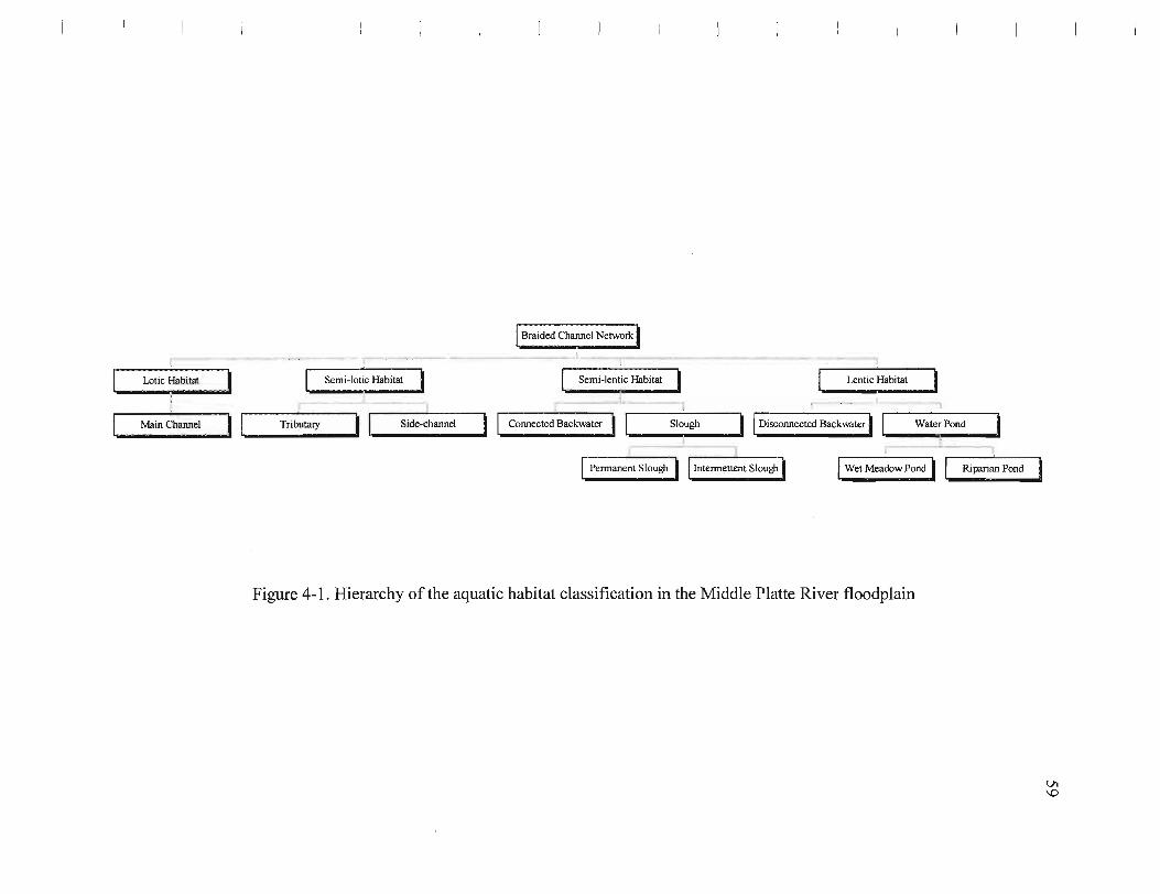
rB;;;d~C;;~;~i'N~~rlCJ
,. ." ,-,"- "," .. , .," ,', ""-"--"'----,, ,I ''"'''' "1'-""'-'-""""
Semi-lentie Habitat I """ '''1 Lentie Habitat I Semi-lotie Habitat
L._,_~ _.~~ ;
,-----'-~----,.. , '
I Intenn~ttent ~!] I Wet Meadow Pond I I Riparian Pond
Figure 4-1. Hierarchy of the aquatic habitat classification in the Middle Platte River floodplain
VI \0

60
4.2 Correlation between the main channel and the riverine habitats
The results of r-values from the correlation analysis are summarized in Table 4-1 , and
the mean r-values are compared by the habitat subtypes and illustrated in Figure 4-2. All
of the correlation analysis results are listed in Table D-1 of Appendix D. The results show
significant differences in surface water levels and groundwater tables versus river stages
(Hs vs. Hr, and Hg vs. Hr) among the habitat subtypes. By comparing the correlation
results across the subtypes (Figure 4-2, Table 4-1), one may see that the degree of
correlation may be depended upon the level of hydrological connectivity between the
main channel (s) and the associated aquatic habitats.
Among the 50 sites analyzed, side-channels (n = 9) have the strongest hydrological
correlations with adjacent main channels in terms of water level change. Mean r-values
were over 0.80 (p< 0.0001) for both the surface water levels and groundwater tables
beneath the riverbed. The mean r-values for the tributary type, in sharp contrast, were
less than 0.40 (p:S0.0343) for surface water, and less than 0.50 (p:S0.0110) for
groundwater (Figure 4-2). These patterns of correlation suggest a significant distinction
in hydrological interaction between the main channel and the side-channel, and the main
channel and the tributary.
The different flow regime in the tributary is a result of inflow from upland, because
the upstream of the tributaries usually link ditches and sloughs. Local intensive rainfall
events and return flow from irrigation may contribute to the tributary flow variation that
is different from the instream flow change in the main channel.

61
Backwater's surface water change, in response to the main channel, was slightly less
active than the side-channel, with mean r-values ranging from about 0.70 to 0.85
(p::;0.0009). Between the two subtypes of backwater habitat, however, there are
differences in the degree of interaction. In average, the disconnected backwater habitats
have a stronger hydrological correlation with the main channels than the connected
backwater habitats. The mean r-values ofthe surface water correlations are 0.6985
(p::;0.0009) and 0.7602 (p<0.0001) for connected backwater and disconnected backwater,
respectively. The groundwater mean rvalues are 0.7891 (p<0.0001) and 0.8493
(p::;0.0000) for connected backwater and disconnected backwater, respectively. The water
body area, shape and fluvial geomorphological features between the two backwater
subtypes may explain their differences in the hydrological interactions. Connected
backwaters generally have longer surface water flow paths and more open surface areas
than those in the disconnected backwaters. Consequently, they may be more adjusted to
influences from the surrounding environment conditions that are less dependent on water
flow changes in the main channel. The disconnected backwaters are found near the main
channel, and have relative smaller patch sizes than the connected backwater channels.
Although they are disconnected from the main channel in surface, the disconnected
backwaters usually are located on highly permeable alluvial substratum, and have a good
subsurface hydrological connection with the main channel.
All other riverine habitats in wet meadow and riparian areas have lower average r
values, less than 0.55 (p::;0.0445) for their surface water correlations with the main
channels. This suggests a weak hydrological connection to the main channel. This is due
to their surface disconnection from the main channel, and relative finer subsurface
sediment layer they have. Intermittent slough type in wet meadows has the lowest
average r-value (0.2779,p~0.0445) (Figure 4-2, Table 4-1).
Statistical results show that 20% of the studied permanent wet meadow sloughs and
50% of the intermittent wet meadow sloughs and riparian ponds have no significant
correlation to the main channels (p> 0.0500).
62
Hydrological connectivity with the main channel seems to playa key role in
characterizing riverine habitat properties. The strength of hydrological response of a
riverine habitat to the main channel instream flow change is directly related to the degree
of its surface water connection with the main channel, as illustrated in Figure 4-3. Fully
surface-connected riverine habitats (side channels) have identical hydro graphs with that
of the main channel. Partially surface-connected backwaters have similar hydro graphs to
the main channel during high stream flow periods, but maintain relatively stable and
shallow water levels when the main channel has low flow rates. The tributaries have
distinct hydrological patterns from the main channel hydro graph because of their
connections with upland runoff and return flows from irrigation. Wet meadow sloughs
generally are not directly connected to the main channel. Subsurface groundwater
discharge and rainfall are the sources of the water supply. They usually drain to
backwaters or side-channels. Disconnected backwaters, ponds in riparian and wet
meadows normally do not have any surface linkage with other aquatic habitats, except
they may receive surface water input from overbank flow occurring during a flood event
(Figure 4-3).

63
After excluding five riverine habitats that were either ephemeral and had non
significant correlation with the main channel, or were profoundly altered by beaver dams,
a total of 40 surface water study sites and 45 groundwater sites were used for further
analyses on the effects of physical environmental factors.

0.9000 ,..--------------------------------,
o Surface water level vs. stream gauge in main channel
0.8000
• Groundwater tab le vs. stream gauge in main channel
0.7000
0.6000
~
~ 0.5000
';a -g ::l 0.4000
0.3000
0.2000
0.1000
0.0000
Habitat Type
Figure 4-2. Comparison of the mean correlation coefficients (Kendallts r-values, a = 0.05) for water level changes between the main channel and the riverine habitat subtypes.
64

Table 4-1. Summary of correlation coefficients (Kendall's r) (a = 0.05) for correlation analysis on water level changes between the main channel and riverine habitats
Kendall's t Habitat Type n Surface Water VS. Main Channel (Hs-Hr) Groundwater VS. Main Channel (Hg-Hr)
Habitat Mean Max Min
Sub-type Prob > I t I Mean Max Min Prob > I t I
Side channel Side channel 9 0.8127 0.9212 0.6626 < 0.0001 0.8152 0.9511 0.6682 < 0.0001
Tributary 5 (2 *) 0.3918 0.7522 0.1658 <= 0.0343 0.4945 0.7703 0.2046 <= 0.0110
Backwater Connected
12 0.6985 0.8640 0.3814 <= 0.0009 0.7891 0.9344 0.6698 < 0.0001 backwater
Disconnected 8 0.7602 0.8561 0.6274 < 0.0001 0.8493 0.9104 0.7484 0.0000
backwater
Slough Permanent
6 (1 *) 0.3773 0.5482 0.1871 <= 0.0194 0.5183 0.6761 0.3054 < 0.0001 slough
I nterm ittent 5 (2 *) 0.2779 0.4021 0.0741 <= 0.0445 0.4964 0.5856 0.3588 <= 0.0046
slough
Pond Riparian pond 4 (1 *) 0.4046 0.5609 0.2471 <= 0.0370 0.5132 0.7893 0.3075 <= 0.0080
Wet meadow 4 (1 *) 0.4949 0.5742 0.4156 <= 0.0002 0.5149 0.5811 0.4486 < 0.0001
pond
Notes: * number of sites where p > 0.05 for the correlation analysis
0\ VI
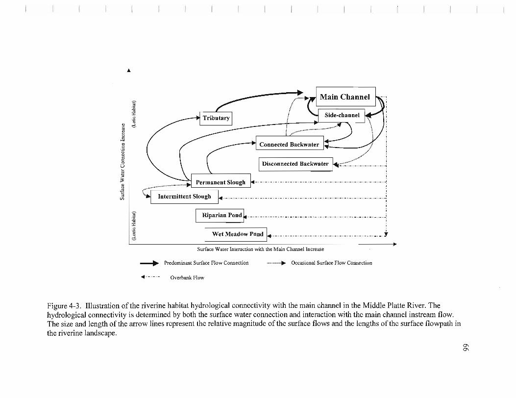
Z' $ :g ::r: <>
'.;:l
1A 0
I e '" <1) .... u
.... .9 0 0 "g
<1)
0 0 0 u ....
~ Connected Backwater
Dj'WDD"'''' Ba<kw.,,, ~.~".:: . .-: .. -~ ... : ... : . _. _.
<1)
-:;; ~ _._ ._._._._._._._._._._._._ ._._._._._._._ ._._._._._.J <1) u
't! ;:s {J)
1? ~
Riparian pond~._ . _. _. _. _ 0 _ 0 _ ' _ 0 _ 0 _ 0 _ . _ . _ 0 _ 0 _ . _ 0 _ ' _ ' _ 0 _ 0 _0 _ ._._ 0 _ 0 _ 0 _ 0
:c I <>
'.;:l
" " e Wet Meadow Pond ~o _0 _ . _ 0 _ o m 0 _ 0 _ 0 _ 0 _ . _ . _ 0 _ 0 _ . _. _0 _ . _ . _ 0 _._ . _. ~
Surface Water Interaction with the Main Channel Increase
---+- Predominant Surface Flow Connection .......... o~ Occasional Surface Flow Connection
.. 0 - • - 0 - Overbank Flow
Figure 4-3. Illustration of the riverine habitat hydrological connectivity with the main channel in the Middle Platte River. The hydrological connectivity is determined by both the surface water connection and interaction with the main channel instream flow. The size and length of the arrow lines represent the relative magnitude of the surface flows and the lengths of the surface flowpath in the riverine landscape.
0\ 0\

67
4.3 Stream widths and habitat locations on the stream-riverine habitat correlations
In addition to the surface hydrological connectivity, a stream channel width and
distance between the stream and associated riverine habitats are among those
environmental factors considered to have an effect on the stream-habitat hydrological
interaction. Zlotnik and Huang (1999) proposed an analytical model of stream-aquifer
interaction that explicitly accounts for the stream width for a partially penetrating stream
with streambed clogging. Given a fixed distance between a stream bank and a
groundwater monitoring well, Zlotnik and Huang's modeling results show that the impact
of stream width on head changes in the monitoring well is significant if the stream width
varies in a range that is less than the distance between the stream bank: and the well. The
effect of the stream width on the head change in the well becomes less significant if the
stream width increases to equal the distance, or wider than the distance between the
stream bank: and the observation site (Zlotnik and Huang 1999, Huang 2000). This model
provides an insight for the riverine landscape study, although the stream width parameter
is not well defined for dynamic braided streams in a floodplain river system. The main
channel of the Middle Platte River is a wide, active, braided channel. Sandbars and
vegetated islands are commonly distributed in the broad stream channel, and their sizes
and shapes change season by season. Thus, measuring the actual stream width is difficult
in practice.
68
In this study, I measured the actual main channel width at two instream flow
conditions: high flow rate (Q = 56.6 m3, or 2,000 cfs) and low flow rate (Q = 11.5 m3
, or
405 cfs). Average stream widths for each of the studied sites was calculated based on
multiple transect measurement data collected in the field across the studied reaches, and
from high resolution digital maps. The overall average main channel width from 45
studied reach sites is 64 m (SD = 56 m) with a range from 8 to 230 m. The distances from
the main channel stream bank to the studied riverine habitats varied from 7 to 670 m with
an overall average distance as 178 m (n=45, SD = 172 m).
In order to exam effect of the riverine habitat location on the strength of the main
channel-riverine habitat interaction, the surface water level r-values were plotted by the
location parameter (Lr). Then, the r-values were fitted with the normal ellipses (p =
0.950) (SAS Institute Inc. 1995) by the habitat types. The results are superimposed in
Figure 4-4. The same procedure was used for the groundwater table r-values, and plotted
as a Lr-rscatter diagram in Figure 4-5. The statistical results are listed in the Table 4-2.
The Figure 4-4 and Figure 4-5 show a similar negative linear relationship between the
r-values and the location parameters for both the surface water (R2 = 0.68, p < 0.0001)
and the groundwater (R2 = 0.71, p < 0.0001). The analysis results and the figures
illustrate two clear spatial patterns: a geographical location pattern of the riverine habitat
types, and a hydrological interaction pattern between the riverine habitats and the main
channel as a function of the location parameter.

69
l,---------~------------------------------------~
0 .9
O.S:
0.3
0.2
O.l4-----~------~----~------~--~~---L--~~--~
o 7 s~ Root[(d+'Wt2)fw]
(Data symbols: • Backwater; + Pond; x Side-channel; and 0 Slough).
Figure 4-4. Clustered riverine habitats by the habitat types, and the habitat surface water 't values fit by the square root of the location parameter [4= (d+w/2)/w].

70
l~-r----~-r-------------------------------.
0.9
0.8
0.4
0 .3 ~ ""'-.
0.2 0 2 3 4 :s .5 1
SqIW"e Root[(d;wt2)lvr]
(Data symbols: • Backwater; + Pond; x Side-channel; and 0 Slough).
Figure 4-5. Clustered riverine habitats by the habitat types, and the habitat groundwater 't values fit by the square root of the location parameter [Lr = (d+w/2)/w].

71
Table 4-2. Statistics of the habitat surface water and groundwater 't values fitting by the square root of the location parameter (Lr) , clustered by the habitat types
Cluster Group n R2 p
Surface Water
All sites 40 0.68 < 0.0001
Side-channel 11 0.89 < 0.0001
Backwater 20 0.22 < 0.036
Slough 6 0.69 < 0.040
Pond 3 nJa nJa
Groundwater
All sites 45 0.71 < 0.0001
Side-channel 11 0.82 < 0.0001
Backwater 20 0.21 < 0.044
Slough 10 0.53 < 0.017
Pond 4 nJa nJa
These results suggest that:
(a) The lateral distributions of the riverine habitat types exhibit different spatial
patterns at the riverine landscape scale, as a function of integrating effect of the main
channel widths and the distances of the habitat geographic positions from the river banks.
The backwater habitat type is positioned close to the main channel, while wet meadow
slough and pond habitat types are located relatively far from the main channel. The side-
channel is a widely distributed habitat type over the riverine landscape. By closely
examining the location of the side-channel type, one may notice that the sites located far
-------------------------------------------------------------------------------

72
from the main channels are those of the tributary subtype, and that located near the main
channel belong to the side-channel subtype. This indicates a general fact that no matter
the size of the associated main channel, tributary subtype habitats are usually located far
from the main channels. So does the pond type, as shown in Figure 4-4 and Figure 4-5.
(b) The geographical location (Lr) affects negatively on the strength ofthe main
channel-riverine habitat interaction at the landscape scale. The strength ofthe
hydrological interaction decreases linearly with increasing square root of the location
parameter.
( c) This effect appears differently at the habitat scale. As shown in Table 4-2, Figure
4-4 and 4-5, it is clearly demonstrate that the location ofthe side-channels affects their
hydrological linkage with the main channel. The habitat l' values of the side-channel
habitats decrease significantly along with increasing of the square root ofthe Lr (R2 =
0.89 and 0.82 for surface water and groundwater, respectively, n = 11 , p < 0.0001). The
pattern is similar to the slough habitat type (R2 = 0.69, n = 6, p <0.04 for surface water,
and R2 = 0.53, n = 10, p <0.02 for groundwater). However, there is no significant Lr-T
relationship for the backwater habitat type (R2 = 0.22, n = 20, P <0.04 for surface water,
and R2 = 0.21 , n =20, p <0.04 for groundwater). This is because the backwaters locate
within similar distances to the main channel (fu = 1 - 2), and have relatively the same,
strong hydrological interactions with the main channel (T = 0.7-0.9). This effect is not
clear for the pond type due to the lack of enough site data for the statistical analysis.
In the case that there was no surface hydrological connectivity to the main channel, the
groundwater linkage seems to be the primary cause determining the strength of
73
hydrological interaction between the stream channel and the adjacent habitats. Other
climatic and land cover factors may also influence the stream-riverine habitat interaction.
4.4 Statistical modeling of the stream-riverine habitat interaction
Simple linear regression models were built to fit water levels in adjacent habitats (Hs
and Hg, m) with main channel discharge (Q, m3/s) for all of the habitats studied, to
evaluate the effects of the main channel regime on water level changes in the adjacent
habitats. The parameters and detailed modeling results are listed in Table D-2 of
Appendix D.
Stepwise multiple regression modeling procedures were used to consider the
contributions of other selected environmental parameters on the stream-riverine
hydrological interaction. The full sets of parameters in the multiple regression models
and the detail results can be found in Table D-3 of Appendix D.
4.4.1 Modeling water level change by the main channel discharge
Table 4-3 summarizes the adjusted coefficient of determination, or Adjusted R-square
(Adj. R2), and p-values by riverine habitat subtypes. The Adj. R2 quantifies the
proportion of variation explained by the regression model on the change of riverine
habitat water level by discharge of a main channel. These Q-H models illustrate that: (1)
the main channel discharge has a significant hydrological impact on side-channel and
backwater habitats (p <0.0001); most of the permanent wet meadow sloughs (p
<=0.0002), wet meadow ponds (p <=0.0003), and tributaries (p <=0.0001); (2) discharge
74
has no statistically significant impact on surface water level change in intermittent wet
meadow sloughs, or isolated water ponds in riparian areas (p >0.0500), but the correlation
of groundwater and discharge is significant in intermittent wet meadow sloughs and
riparian ponds (p <0.0001).
Both the surface water regression (Q-Hs) models and the groundwater regression (Q
Hg) models reveal an identical trend in the significant influence of main channel
discharge on adjacent habitats, i.e. side-channel > connected backwater > disconnected
backwater > tributary > wet meadow pond and permanent slough > intermittent wet
meadow slough > isolated riparian water pond (Table 4-3). This trend is similar to the
results ofthe correlation analysis between water level elevations from main channel
stream gauges and water levels monitored in the riverine habitats. Here it can be
examined by comparing the Adj . R2 values of the models for different riverine habitat
types, and by contrasting that to the surface water models and the groundwater models.
It is not surprising that both of the surface water-discharge (Q-Hs) model and the
groundwater-main channel discharge (Q-Hg) model in the side-channel habitats
explained more than 90% of the variation in adjacent habitats by main channel discharge
alone, because the side-channel subtype habitats are the most closely tied hydrologically
with the main channel. On other hand, applying the regression model on the tributary
subtype, the main channel discharge alone could only explain about one-third ofthe
water level variation in the tributary habitats. These results indicate quantitatively the
hydrological differences between the tributary and the side-channel subtypes. Thus, it is
75
necessary to separate the tributary habitat from the side-channel habitat type, and classify
it as a separate type.
The regression models also perform well (the mean Adj . R2 varies from 68.2% to
88.3%) for two subtypes of backwater habitat (Table 4-3). The Q-H models predict water
level variation in the connected backwater habitat better than in the disconnected
backwater subtype. This reflects the hydrological connectivity as a cause to the
hydrological interaction between the habitats and the main channel. The fact that the
backwater habitats' adj. R2 value are generally lower than those for the side-channel
habitats may imply a declining strength in the hydrological interaction between the main
channel and the backwater habitats as compared to the side-channel habitats.
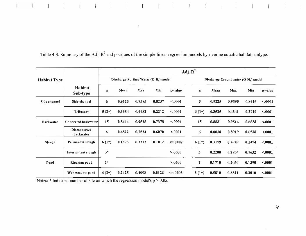
Table 4-3. Summary of the Adj. R2 and p-values of the simple linear regression models by riverine aquatic habitat subtype.
Adj. R2
Habitat Type Discharge-Surface Water (Q-H,) model Discharge-Groundwater (Q-Hg) model
Habitat Mean Max Min n
Sub-type p-value n Mean Max Min p-value
Side channel Side channel 6 0.9125 0.9585 0.8237 <.0001 5 0.9225 0.9590 0.8416 <.0001
Tributary 5 (2*) 0.3384 0.4482 0.2212 <.0001 3 (1 *) 0.3525 0.4341 0.2710 <.0001
Backwater Connected backwater 15 0.8614 0.9528 0.7378 <.0001 15 0.8831 0.9514 0.6838 <.0001
Disconnected 6 0.6822 0.7524 0.6070 <.0001 6 0.8038 0.8919 0.6538 <.0001
backwater
Slough Permanent slough 6 (1 *) 0.1673 0.3313 0.1012 <=.0002 6 (1 *) 0.3179 0.4749 0.1474 <.0001
Intermittent slough 3* >.0500 3 0.2200 0.2834 0.1632 <.0001
Pond Riparian pond 2* >.0500 2 0.1710 0.2030 0.1390 <.0001
Wet meadow pond 4 (2*) 0.2425 0.4098 0.0126 <=.0003 3 (1*) 0.5810 0.8611 0.3010 <.0001
Notes: * Indicated number of site on which the regression model's p > 0.05.
-.....l 0'\
77
The Q-Hs models of the slough and pond habitats have very low Adj. R2values. More
than half of the studied wet meadow slough and pond habitats (8 of 15 study sites) did
not have a statistically significant relationship (p > 0.0500) between their surface water
changes and the main channel discharge changes. The Q-Hg models ofthe slough and
pond habitats show significant relations between the main channel discharge and the
groundwater table changes (Table 4-3).
The regression models explain more of the variation in the groundwater table than
surface water level changes (Table 4-3). This modeling feature suggests that there is a
stronger relative hydrologic response of riverine habitats through the groundwater flow
paths between the main channel and the riverine habitats than that through surficial flow.
Degree of difference varies among the habitats, and it seems to have been negatively
associated with the surficial hydrological connectivity betw~en main channel and
adjacent habitats. For instance, for those types of habitats maintaining surficial
hydrological linkage with main channels, such as the side-channel, tributary, and
connected backwater habitats, there was only a 1.0 to 2.2 % difference in Adj. R2 values
between the surface water and groundwater regression models (Table 4-3). This means
that the Q-Hg regression models work slightly better than the Q-Hs models in explaining
hydrological variations associated with the main channel discharge.

78
The hydrological characteristics of the sloughs contrast with the hydrological features
of other subtypes that surficially separated from the main channel, such as disconnected
backwater, sloughs, and ponds. For these 'non-surficially linked' habitats, the differences
in mean Adj. R2 values between surface water regression models and groundwater
regression models are significant. The calculations for these differences yield 12.2 %,
15.1 %,22.0 %, 17.1 %, and 33.9 % for disconnected backwater, permanent slough,
intermittent slough, riparian pond, and wet meadow pond, respectively). These results
suggest the relative importance of the main channel discharge to groundwater in diverse
riverine habitats.
The simple discharge-water level regression model poorly describes the hydrological
response in a wet meadow habitat. This suggests that other environmental factors, such as
temperature, precipitation, and evapotranspiration may be responsible for variations in
water level in wet meadows. A multiple regression modeling is needed to consider other
possible factors.
4.4.2 Stepwise multivariate regression models
The series of multiple linear regression models generalized from the stepwise
regression identified eleven combinations of the four primary environmental variables
(Q, T, P, and ET) (Table 4-4). The models identify the main hydro-climatic factor(s) that
control the hydrological process in each of the riverine habitats. These combinations for
modeling hydrology of the riverine habitats may also reflect the landscape heterogeneity
In habItat scale, and the compiexity of hydrological processes within the riverine
landscape.
79
A summary of the Adj. R2 values ofthe models by habitat subtypes is given in Table
4-5. By comparing the Adj. R2 values in Table 4-3 and Table 4-5, one may find that the
multiple regression models in general provide: (a) only a slight improvement (0.6- 5.6 %)
over the simple linear regression models in explaining water level variations in side
channel and backwater habitats; (b) an 11- 32 % improvement in the interpretation of the
variation for ponds in riparian and wet meadow slough habitats; ( c) little advantage for
ponds in wet meadows; and, (d) The climate variables contribute differently to the habitat
subtype of in explaining variation in water level changes. It shows that the temperature
factor contributes more than the ET factor does. This is most likely due to the process of
direct evaporation from the open surface water of the riverine habitats, which is strongly
related to the temperature factor. No direct on-site ET measurement was conducted. The
ET data used in this study were calculated values based on weather observation data
collected in areas with dominant agricultural land cover and located several kilometers
from the river floodplain (Hubbard 1992; Robinson and Hubbard 1990). This maybe
another reason for the relatively weak correlationship between the ET and the water level
change in the riverine habitats. Furthermore, the linear regression model cannot model
water level change at several study sites due to significant natural or human disturbances
and other biological impacts such as beaver damming.

80
Table 4-4. Combinations of explanatory variables in the linear regression models generalized by the stepwise multiple regression processes, and numbers of modeled riverine habitats by each of the associated models.
Variables in Number
model of sites Type and landscape features of the modeled riverine habitats
modeled
(1) Most of side-channels and some of backwaters immediately adjacent to Q 14 main channels, and have surface water connection with the main channels; (2)
A few of wet meadow ponds near the main channel.
Some ofsmal! side-channels and most of backwater and wet meadow habitats Qand T 12 close to the main channel with large open space and bare ground, such as
sandbars.
Longer side-channels, tributaries, backwaters, and wet meadow sloughs that QandP 7 have relative large catchments, and closed canopy of riparian belts or
woodland along these riverine aquatic habitat channels.
Q andET 1 A beaver pond built in a tributary reach with open area and shrubs c~ver.
Q, T, and P 4 Longer backwaters and wet meadow sloughs with relatively large catchments, and no closed riparian canopy.
Q, P, and I
A long side-channels that have relative large catchments, and shrubs dominant ET riparian, no closed canopy.
T 2 Ponds far from main channels with open space and bareground, no canopy.
TandP 2 Longer wet meadow sloughs that have relative large catchments, far from main channel, and no closed riparian canopy for most of the habitats.
P 1 A smal!lowland pond in riparian far from main channel.
No suitable 6
Tributary and wet meadow pond far from main channel, with silt, or sandy clay variable stratum.
-- ---------------------------------------------------

Table 4-5. Summary of the Adj. R2 and the p-values of the multiple linear regression models by the subtypes of the riverine habitats
Habitat Type Surface water multiple linear models
Habitat Mean Max Min n
Sub-type
Side channel Side channel 6 0.9186 0.9644 0.8545
Tributary 5 (2*) 0.3939 0.5615 0.2747
Backwater Connected backwater 15 0.8813 0.9528 0.7775
Disconnected 6 0.7194 0.7909 0.6625
backwater
Slough Permanent slough 6 (1 *) 0.3218 0.4760 0.1012
Intermittent slough 3 (2*) 0.3185 0.3185 0.3185
Pond Riparian pond 2 (1*) 0.3013 0.3013 0.3013
Wet meadow pond 4 (2*) 0.2425 0.4098 0.0126
Notes: * Indicated number of site on which the regression model's p > 0.05.
Adj. R2
p-value n
<.0001 5
<.0001 3 (1 *)
<.0001 15
<.0001 6
<=.0002 6 (1 *)
<=.0001 3
0.0004 2
<=.0003 3 (1 *)
Groundwater multiple linear models
Mean Max Min
0.9287 0.9590 0.8722
0.3757 0.4341 0.3173
0.8954 0.9514 0.7158
0.8267 0.9116 0.6735
0.4270 0.6371 0.2611
0.3716 0.5474 0.2505
0.3104 0.3695 0.2512
0.5888 0.8765 0.3010
p-value
<.0001
<.0001
<.0001
<.0001
<.0001
<.0001
<.0001
<.0001
00 -
4.5 Spatial patterns of the riverine landscape as response to hydrological changes
4.5.1 Components of the riverine landscape
82
Landscape ecology considers spatial and temporal attributes of landscapes and links
spatial patterns to processes when addressing ecosystem integrity (Fortin 1999; Pickett
and Cadenasso 1995; Wiens 2002; Wiens et al. 1993). Landscape attributes refer to patch
quantity and quality, patch structure, and patch dynamics (Leuven and Poudevigne 2002).
Figure 4-6 and Figure 4-7 are land-cover maps exported from my GIS-based spatial
explicit models (SEMs) generated based on two digital images. They were achieved on
the dates when there were distinct river discharges. One image was taken in October
1995 when discharge was 56.6 m3/s (2,000 cfs), and represented a high instream flow
management scenario (Bowman 1994; Bowman and Carlson. 1994; CNPPID 1998, 1999;
CPNRD 1990, 1992; Farrar 1992; Hill et al. 1991; NDWR 1992, 1998; NGPC 1993b,
1997). Another image was taken in August 1998, when discharge was 11 .5 m3 Is (405
cfs), and represented a low instream flow scenario. They cover one of the management
properties of the U.S. FWS and adjacent areas.
Land cover was classified into six categories, based on digital values of the land cover
spectral data. Landscape components were recognized based on the land cover
classification and field surveys. In the present study area they include hierarchically
linked aquatic habitat patches (such as main channel deep water patch and shallow water
patch, instream sandbar patch, side channel patch, riverine backwater patch, riparian
pond patch) and mosaics of terrestrial patches of riparian woodland, grassland, cropland,

83
etc. The habitat attributes were measured and quantified at 1 and 2 .. meter resolution, and
aggregated to the habitat scale.
_ Tree DShmb o Gnlss
E1 Baregrolilld Sh ... llowWiJler
_ Deep W.lter
200 o 200 Meters ~~iiiiii~~~~
Figure 4-6. Land cover map exported from a GIS based digital riverine landscape classification model that covers a management property and adjacent areas at a reach of the Middle Platte River, 4 km southeast of Kearney, Nebraska. Original color infrared photograph was taken by U.S. FWS (1995) on October 25, 1995, when Q = 56.6 m3/s (2,000 cfs), representing a high instream flow management scenario.

_ Tr .. _ Water o Shrub D Grass D Bareground o DeepWater
84
Figure 4-7. Land cover map exported from a OIS based digital riverine landscape classification model that covers a management property and adjacent areas at a reach of the Middle Platte River, 4 km southeast of Kearney, Nebraska. The original color infrared photograph was taken by U.S.O.S. (1998) on August 1998, when Q = 11.5 m3/s (405 cfs), representing a low instream flow scenario.

85
4.5.2 Spatial analysis of the riverine hydrological patterns
Aquatic habitat patches and hydrological networks were extracted from the GIS
models to make new aquatic patch theme maps as shown in Figure 4-8 (a) and (b), and
Figure 4-9 (a) and (b). My analyses were focused on one side-channel and one backwater
channel on the north bank of a branch of the main channel.
Groundwater table contour lines were generated based on the water-table monitoring
data in eight piezometers and a detailed field topographical survey carried out along three
transects and the stream banks. They were superimposed on the aquatic patch theme
maps as displayed in Figure 4-8 (b), and Figure 4-9 (b). The arrows on the maps indicate
the groundwater flow paths.
Figure 4-8 (b) shows that during the high instream flow period, the river main channel
discharged to the riverine aquifer laterally, and the groundwater flow paths went toward
to the backwater and the side-channel habitats. Figure 4-9 (b) shows a relatively opposite
groundwater flow path pattern during the base flow period. The lateral groundwater
flowed paralleled the main channel flow direction and recharged the river at the
downstream side of the study area. Parts of the groundwater flow went through the side
channel. No groundwater discharged to the side-channel due to the lower water tables in
the riverine aquifer.
The riverine surface water and groundwater hydraulic gradients in the riverine aquifer
may be determined using the calculation method presented by Heath (1983), by
measuring: (a) the differences of surface water levels between the stream channel (Hr)

and the adjacent riverine backwater or the side-channel habitats (Hs) that connects with
the stream; and (b) the difference between the stream gauge heights (Hr) and the
groundwater tables underneath the adjacent riverine habitat (Hg), that mayor may not
have direct surface hydrologic connection with the stream; and (c) the water flow
distance from the stream to the studied riverine habitats.
4.5.3 Spatial analysis of the riverine habitat patterns
86
Landscape indices were calculated using ArcView's Patch Analyst extension (Elkie et
al. 1999) at both landscape and habitat scales. Results are summarized in Table 4-6. By
comparing the landscape indices at the low instream flow condition with that at the high
flow rate, one may calculate the dynamics of the habitat patches and explore patterns. In
the study area, the total area of the aquatic habitats, expressed as patch class area in the
patch analysis, declined by 34 %, while the number of patches increased by 135 %. These
changes indicate a more fragmented landscape with reduced aquatic habitat areas
appeared under the low discharge condition. Mean habitat patch size decreased by 72 %,
from 234 m2 down to 65.7 m2. The smaller patch size standard deviation in the low flow
conditions as shown in Table 4-6 suggests that the sizes of the aquatic habitat patches
was more similar under low flow conditions than at a high rate of flow. Corresponding to
the habitat fragmentation, total patch edges and patch edge density increased 59 % and
141 %, respectively. Due to increasing numbers of patches, the mean patch edges
decreased about 32 %. The mean patch shape index (MSI) is used to describe patch shape
complexity. It is an averaged perimeter-area ratio for all patches in the landscape, i.e. the

87
mean patch shape index compares a patch shape with a square, and it is greater than 1
(Elkie et al. 1999). The larger the MSI, the more complex a patch shape is. Thus, the MSI
results in this area indicate that the shapes of the aquatic patches were less complex under
dry conditions than when the instream flow rate was high. Another important spatial
difference, found by comparing total cover areas on each type of habitat in Figure 4-8 and
Figure 4-9, is that when flow rate in the main channel dropped to its base-flow level,
more patches in side-channel and backwater habitats went dry than that in main channels.
The consequence of reduction in habitat patch size and density in riverine habitats causes
a decline of the riverine hydrological connectivity. Furthermore, lowering river water
levelled to change of the local groundwater flow paths. As the result, the riverine water
was drained and discharged to the main channel until they went dry. These results, based
on two hydrological scenarios (high and low instream flow rates), demonstrate that the
landscape patterns and hydrological connectivity of riverine habitats are dynamic, and in
response to the hydrologic regime in the main channel.

.. - . ' :", '/' .. ::-~~. • " '.1. >.'/::', ::-,' ,'!i.;,-'l . .' _. ..~ .,.. , .. , ' -) .. . ..".
Legend
Braided stream network _ Su,hc.",n. t
o Sudbals and fkl odplli'l
_ Study., ••
Control poilt
Figure 4-8 (a). A quatic habitat patches and braided stream networks under a high instream flow condition were extracted from GIS models to make this riverine landscape map at riverine landscape/reach scale. Rectangular area in center of the map, enlarged in figure (b), was detailed surveyed for topography. Red dots mark surveyed piezometers, stream gauges, and shorelines of the streams and banks. The river flows from west to east in the map.
88

100
.,. ... ,..-o 100 200 - - 300 Meters
-- -
89
Legend
Braided stream network
_ Surflc • • ater
o hndb:ars Jlnd toodpbl in
Corotrol point
Figure 4-8 (b). Aquatic patch theme map at habitat patch scale, with groundwater table contour lines superimposed on the aquatic patch theme map. Arrows represent groundwater flow paths. This map represents a high instream flow condition (Q=56.6 m3 or 2,000 cfs) in spring and fall. The river flows from west to east in the map.
-----

" . 1. ...
900 0 900 1800 Meters
~~--~~~~~----~
Legend
Bra ided stream network -o - Siilndo ;jl rl ~ndf loodp l.i in
Control point
90
Figure 4-9 (a). Aquatic habitat patches and braided stream networks under a low instream flow condition extracted from GIS models to make this riverine landscape map at landscape/reach scale. Rectangular area in center of the map, enlarged in figure (b), was a detailed surveyed for topography. Red dots mark the surveyed piezometers, stream gauges, and shorelines of stream and banks. The river flows from west to east in the map.

/I e _ ... ~
0 ' . ...... l "r ,.-/ '- ~ ' . "- - , .
/ ~ ~ ~ \ /" --
~ ~
• . ~. OJ / .1 ~' I ~ • \"
~
100 o 100 200 300 Meters - --- -
N
W* E S
Legend
Braided stream network _ SlrfIc..at.r
<8 S:mdb-ars and ioodpblln
_ Ou p .at.r In main ohann*1
91
Figure 4-9 (b). Aquatic patch theme map at habitat patch scale, with groundwater table contour lines superimposed on the aquatic patch theme map. Arrows represent the groundwater flow paths. This map represents a low instream flow condition (Q=11 .5 m3 or 405 cfs) in a sUIilmer dry season. The river flows from west to east in the map.

Table 4-6. Comparison of landscape indices for riverine habitats changes under different hydrological processes at the landscape scale.
Landscape Indices High Stream Flow Low Stream Flow Change (Elkie et al. 1999) (A) (B) (B - A)
Total patch class area (CA, m2) 585,878 387,000 -34%
Number of patches (NumP) 2504 5893 +135 %
Mean patch size (MPS, m2) 234 65.7 -72 %
Patch size standard deviation (PSSD) 0.95276 0.25692 -73 %
Total patch edges (TE, m) 96912 154354 +59%
Patch edge density (ED, mll04m2) 1654.13 3988.44 +141 %
Mean patch edges (MPE, mlpatch) 38.71 26.19 -32 %
Mean patch shape index (MSI) 1.3441 1.3218 -2%
92

93
Chapter 5. Results and Discussions (II): Physicochemical Heterogeneity
Understanding the distribution pattern of surface water physicochemical properties is
very important for river ecology, and is critical for the ecological risk assessment of the
river ecosystem. The landscape of the Middle Platte River floodplain is a diverse and
dynamic mosaic of habitat patches. These patches have distinctive features of hydrology,
geomorphology, land cover, and land use that may affect or determine physical and
chemical characteristics of surface water. Thus, one may expect that the distribution of
physico-chemical properties in surface water of the riverine habitats would reflect the
habitat spatial heterogeneity. However, temporal variability of surface water in the
riverine habitats is significant given their dynamic hydrological interactions with the main
channel (Wu 1999c). The research questions are: (1) are the physicochemical properties
of riverine aquatic habitat types significantly different from each other? And (2) what are
the spatial and temporal patterns of physicochemical parameters across the habitat types?
To investigate the heterogeneity of the river landscape from the physicochemical
perspective, the spatial patterns of physicochemical heterogeneity were examined using
the habitat types classified by the criteria listed in Table 3-3 in the chapter 3.

94
5.1 Physical and chemical properties of surface water in the riverine landscape
5.1.1 Daytime temperature
Temperature and water current are two of the major environmental factors that
directly affect the activities of aquatic organisms (Allan 1995; Goldowitz 1996a~ 1996b).
Field measurements (n = 434) show that the mean daytime temperature of surface water
in the Middle Platte River, including the main channel and adjacent habitats, was 18.8 °C
(65.8 F) during the study period. The temperature varied from 15 to15.6 °C (59 to 60 F)
in spring, 21.7 to 25.0 °C (71 to 77 F) in summer, and 9.3 to 10.9 °C (49 to 52 F) in the
fall (Table 5-1, Fig 5-1). Analysis of variance (ANOVA) showed there was no significant
difference in the mean daytime temperature among the nine subtypes of aquatic habitat (F
(8,113 .93) = 1.65, P = 0.1191. Table 5-2, Figure 5-2, Figure 5-3). Due to the direct
connection of side-channels and backwaters with main channels, there were only slight
mean temperature differences in these habitats. Temperatures in the tributary was more
than 1 °C (2 F) higher than that of the main channel; by contrast, the mean daytime
temperature in backwater was 0.6-1 °C (1 F) lower than in the main channels (Table 5-2).
These differences may be the effect of different land cover, groundwater discharge,
current velocity, and hydrological conditions. Permanent wet meadow sloughs, where
groundwater is the main water source, had the lowest mean daytime water temperature
among the nine habitat types, about 2.4 °C (4 F) lower than that of the main channels,
which suggests groundwater as the dominant source of water input. Intermittent slough

95
and shallow wet meadow ponds had higher mean temperatures than the main channel and
other habitat subtypes due to their shallow and motionless water bodies (Table 5-2,
Figure 5-2).
The spatial pattern of the distribution of mean daytime temperature in surface water
across aquatic habitats of the Middle Platte River was illustrated by comparing the mean
values of the habitat subtypes. This pattern changed with season (Figure 5-3). In spring,
the distributions were nearly same in the nine habitat subtypes (F test, p > 0.05). The
temperature in the main channel was about 1 °C to 3 °C lower than in the riparian
habitats. In summer, a step-type distribution pattern occurred from the main channel (23-
28°C) to the wet meadow sloughs (20-24 0C), with the exception of intermittent wet
meadow sloughs and riparian ponds, where in shallow, calm water mean temperatures
rose to 28-32 DC. During high river flow periods in June and August 1997, water
temperature in the main channel was no higher than that in the side channel (Figure 5-3).
In the fall, the difference in mean water temperatures among the habitat subtypes was
lessened, with those in the riparian pond and the backwater types being the highest and
those in the sloughs being the lowest among the habitat subtypes.

Table 5-1. Temporal changes in physical and chemical properties (mean ± SD) of surface water in the Middle Platte River during the
study period, 1996-1 998 (n = 434). Note: no salinity measurement was conducted in May 1996.
Date Temperature
pH DO (mg/L) Conductance
Salinity (ppt) n (OC) (25°C, ~s/cm) _._. ____ ._ •••• __ • • _ ••• __ • __ ._. ____ • __ ._ •• __ ••••• _ ••• ~._ .. __ u_ .................. -..... --... -~- .... - .... ---....... -.. - ... _ ........
May-96 33 15.1 ±2.0 7.7 ± 0.4 7.57 ± 2.39 927 ± 158
Aug-96 63 25 .1 ± 5.0 8.0± 0.6 7.54 ± 3.38 956 ± 236 0.5 ± 0.1
Apr-97 51 15.6 ± 2.9 8.4 ± 0.3 11.07 ± 3.33 984 ± 182 0.5 ± 0.1
Jun-97 61 23.1 ±4.5 8.0 ± 0.4 8.21 ± 2.97 985 ± 140 0.5 ± 0. 1
Aug-97 66 23.6 ± 3.5 7.9 ± 0.4 7.44 ± 2.91 1026 ± 289 0.5 ± 0.1
Oct-97 63 10.9 ± 2.1 7.8 ± 0.5 8.57 ± 2.94 1020 ± 213 0.5 ± 0. 1
Jun-98 59 21.7 ± 2.7 8.1 ± 0.5 9.11 ±3.42 950 ± 127 0.5 ± 0.1
Nov-98 40 9.3 ± 1.5 8.0± 0.7 9.12 ± 2.81 1054 ± 265 0.5 ± 0.1
\0 0\

Table 5-2. Spatial heterogeneity of physical and chemical properties (mean ± SD) of surface water in the Middle Platte River during
the study period, 1996-1998 (n = 434), summarized by aquatic habitat subtype.
Habitat Temperature
pH DO (mg/L) Conductance
Salinity (ppt) n (OC) (25°C, Ils/cm)
Main channel (MC) 112 18.7±6.6 8.4 ± 0.3 9.50 ± 1.32 930 ± 58 0.5 ± 0.0
Side-channel (SC) 31 19.0 ± 6.3 8.3 ± 0.4 9.49 ± 1.56 933 ± 54 0.5 ± 0.0
Tributary (TB) 51 20.0 ± 7.1 8.1 ± 0.4 10.20 ± 3.59 973 ± 148 0.5 ± 0.1
Connected backwater 83 18.1±6.0 7.9 ± 0.4 8.20 ± 3.35 1020 ± 148 0.5 ± 0.1
(CB) Disconnected backwater
41 17.4±6.1 7.6 ± 0.4 5.73 ± 3.98 1052 ± 194 0.5 ± 0.1 (DB)
Permanent slough (PS) 51 17.6 ± 5.7 7.7 ± 0.4 7.56 ± 3.22 1107 ± 288 0.6 ± 0.1
Intermittent slough (IS) 15 21.6±9.3 7.5 ± 0.8 8.54 ± 3.97 774 ± 395 0.4 ± 0.2
Wet meadow pond (WP) 29 22.3 ± 8.4 8.0 ± 0.8 8.82 ± 3.58 1034 ± 422 0.5 ± 0.2
Riparian pond (RP) 23 17.6±5.3 7.8 ± 0.7 6.87 ± 3.91 984 ± 228 0.5 ± 0.1
\D -.....l

98
32.5
30.0
27 .5
25 .0
22.5
G '"- 20.0 " ~ = ~ Co 17.5 e ~
15.0
12.5
10.0
7.5
5.0
May-96 Aug-96 Apr-97 Jun-97 Aug-97 Oct-97 Jun-98 Nov-98
Date
Figure 5-1. Seasonal change in surface water mean (+ SD) daytime temperature (OC) in
the Middle Platte River during the study period, 1996-1998 (n = 434)_
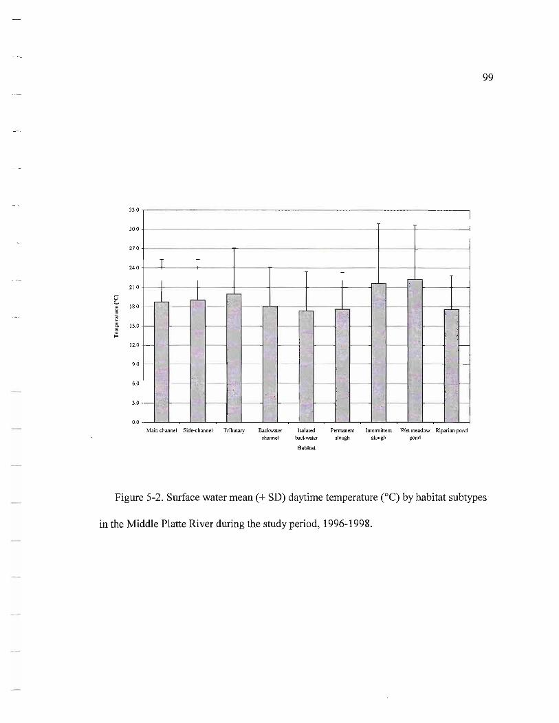
99
33.0
30.0
27.0
24.0
21.0
U e..-" 18.0 .. " ~ C- 15.0 ~ ""
12.0
9.0
6.0
Main channel Side-channel Tributary Backwater Isolated Pennanent Intermittent Wet meadow Riparian pond channel backwater slough slough pond
Habitat
Figure 5-2. Surface water mean (+ SD) daytime temperature (OC) by habitat subtypes
in the Middle Platte River during the study period, 1996-1998.

SubHabitat 11. Me 5. IB
SdlHobiW by Dolo
. TB
. IS sc
. WP PS
9. RP . BW
Figure 5-3. Spatial patterns of surface water mean daytime temperature eC) in the
100
habitat subtypes in the Middle Platte River, and their seasonal changes during the study
period, 1996-1998.
Under similar weather condition, water depth, source of water input, and land cover of
the riverine habitats play main roles in change of the temperature pattern. As my results
showed, side-channel, tributary, and most backwater bodies were shallower « 0.3 m)
than the main channel (normally 0.30 to 0.80 m deep). Current velocity was typically

101
0.15-0.25 m/s in these habitats; while in the main channel it was usually over 0.30 m/s
under normal flow conditions (Table 3-1). Side-channel and tributary channel habitats
had narrow open channels with denuded or sparsely covered sandbars. The exposed sandy
surface in the side-channel contributes to increasing the temperature of a side-channel
faster than that in the main channel.
Most backwater bodies are disconnected from the main channel. Instead of direct
inflow from surface channels, backwater bodies receive seepage from riverbanks, or
recharge from subsurface groundwater. Cooler shallow groundwater recharge can reduce
the surface water temperature of a backwater and wet meadow slough habitat. Also, in
backwater habitat, vegetative cover was denser than that in the side-channel. Canopies of
cottonwood, willow, and dogwood along the shoreline shaded most of the backwater
areas, and probably reduced sun time in backwaters.
During a summer dry season, the river level in main channels dropped to about 30 cm
or less, and large areas of sandbars appeared. The mean surface temperature was higher in
this case than that in side channels.
5.1.2 Hydrogen ion concentration (PH)
Hydrogen ion concentration is one of the most important and frequently used
chemical indicators in study of aquatic habitat, because many chemical phases and
processes are pH-dependent (Eaton et al. 1995), for example, the bicarbonate buffer
system of freshwater, which is critical to the maintenance of life (Allan 1995).
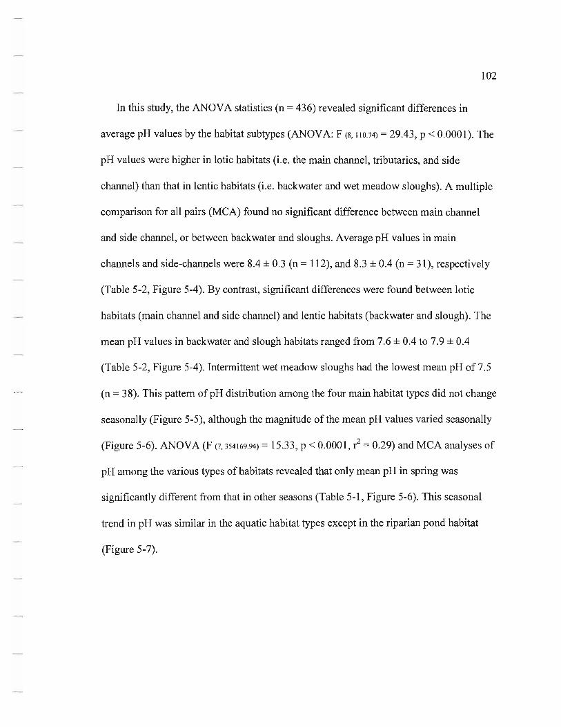
102
In this study, the ANOVA statistics (n = 436) revealed significant differences in
average pH values by the habitat subtypes (ANOVA: F (8, 110.74) = 29.43, P < 0.0001). The
pH values were higher in lotic habitats (i.e. the main channel, tributaries, and side
channel) than that in lentic habitats (i.e. backwater and wet meadow sloughs). A multiple
comparison for all pairs (MCA) found no significant difference between main channel
and side channel, or between backwater and sloughs. Average pH values in main
channels and side-channels were 8.4 ± 0.3 (n = 112), and 8.3 ± 0.4 (n = 31), respectively
(Table 5-2, Figure 5-4). By contrast, significant differences were found between lotic
habitats (main channel and side channel) and lentic habitats (backwater and slough). The
mean pH values in backwater and slough habitats ranged from 7.6 ± 0.4 to 7.9 ± 0.4
(Table 5-2, Figure 5-4). Intermittent wet meadow sloughs had the lowest mean pH of7.5
(n = 38). This pattern of pH distribution among the four main habitat types did not change
seasonally (Figure 5-5), although the magnitude of the mean pH values varied seasonally
(Figure 5-6). ANOVA (F (7, 354169.94) = 15.33, P < 0.0001, r2 = 0.29) and MCA analyses of
pH among the various types of habitats revealed that only mean pH in spring was
significantly different from that in other seasons (Table 5-1, Figure 5-6). This seasonal
trend in pH was similar in the aquatic habitat types except in the riparian pond habitat
(Figure 5-7).

103
9.00 ,---------- ------------ - ------------,
8.75 -j-------- - ------------ - - - - -------'l'------ - ---j
8.50 -j--+-------1I------=,--------------------I- - - -I----j
8.25
8.00
:a. 7.75
7.50
7.25
7.00
6.75
Main channel Side-channel Tributary Backwater Isolated Pennanent Intennittent Wet meadow Ri parian pond channel backwater slough slough pond
Habitat
Figure 5-4. Mean (+ SD) pH value by habitat subtypes in the Middle Platte River
floodplain during the study period, 1996-1998 (n = 436).

SubHabitat . 1. MC . 6. PS
SIiIBibitaiby Dat •
2. SC 7. IS
. TB D 4. BW WP . 9. RP
104
5. IB
Figure 5-5. Spatial distribution patterns of mean pH by habitat subtypes in the Middle
Platte River floodplain, and their changes during the study period, 1996-1998.
9.00
8.75
8.50
8.25
= "-
8.00
7.75
7.50
May-96 Aug-96 Apr-97 1un-97 Aug-97 Ocl-97 1un-98 Nov-98
Date
Figure 5-6. Seasonal change in mean (+ SD) pH in the Middle Platte River during the
study period, 1996-1998 (n = 436).
105
- ---- - --- - ----- ----- - - - ------

1. IlC 3. TB 2 . SC 6. PS 4.BW 5. lB 1. IS 8. WP 9. RP
Date o Jun-97
Figure 5-7. Seasonal change in mean pH within habitat subtypes in the Middle Platte
River, during the study period, 1996-1998.
106
107
5.1.3 Dissolved Oxygen
Two important biological processes alter dissolved oxygen (DO) concentrations in
water: photosynthesis and respiration of aquatic organisms. Since water temperature and
current vary among the aquatic habitats and with season as shown in previous sections, it
is not surprising that there was significant variation in DO concentrations in the study
areas, due to changes in water temperature, depth, current velocity, and biological
activity. The average concentration of surface water DO for all habitats studied was 8.5
mglL during the study period (n = 423). ANOVA (F (7, 160.73) = 6.92, P < 0.0001) and
MCA analyses showed that mean DO in spring was significantly different compared to
that in summer. The highest DO occurred in spring. Seasonal changes of mean DO in
surface water varied from 10.9 mgIL in spring to 7.0-8.3 mgIL in summer, with up to 9.2
mglL in fall (Table 5-1 , Figure 5-8).
ANOVA (F (8, 103.36) = 8.3, P < 0.0001), and MCA analyses suggested significant
differences in the mean dissolved oxygen concentrations of surface water among the four
habitat types, especially between the main channel and side channel group and the
backwater and slough group. Statistical results (Table 5-2, Figure 5-9) indicated that
mean DO concentrations in the main channel and side-channel with fast flowing water
were 9.5-10.2 mglL; in isolated backwater habitat, mean DO was 5.7 mglL; sloughs in
wet meadows had lower DO (7.6 mg/L), because of subsurface groundwater input and
relatively static conditions of the water body (Table 5-2, Figure 5-9). Variation in DO

108
concentrations was low in the main channel (SD= 1.32) relative to those in backwater
(SD=3 .98) and in wet meadow slough habitats (SD=3.97). This pattern probably results
from abundant algae and macrophytes in the relatively calm environment of backwaters
and wet meadow sloughs.
Spatial distribution patterns of mean dissolved oxygen concentrations in four main
types of aquatic habitat changed seasonally during the study period. Three patterns of DO
distribution in the four habitats repeatedly occurred during the study periods (Figure 5-
10):
Pattern 1 (spring DO pattern): the side channel and tributary types had the highest DO
levels, while the slough types had the lowest. This pattern happened in all of the three
spring seasons studied (i.e. 1996 - 1998).
Pattern 2 (summer DO pattern): lotic habitats had the highest DO concentrations,
while the slough had the lowest. This pattern occurred in summer (1996 - 1997).
Pattern 3 (fall DO pattern): backwater habitat had the lowest DO; other habitats had
similar DO levels. This pattern happened in fall 1997 and 1998 (there was no water
sampling in fall 1996).
DO variation in the intermittent slough and pond habitats was extremely high, with no
evident pattern.

15.00 ~--.-.... -.. -........... - ....... - .... --.... --.---.... - ... -.------............. ----....... -...................... -........ -.--_.-................... _-.-.-..... -._---........ __ ..... _ .. .
13 .00 +----------+--------------------~
~ .!
11.00
= ~ .. ~
0 i! ~
~ 9.00 is
7.00
5.00
May-96 Aug-96 Apr-97 Jun-97 A ug-97 Ocl-97 Jun-98 Nov-98
Date
Figure 5-8. Seasonal change in mean (+ SD) dissolved oxygen concentration in the
Middle Platte River during the study period, 1996-1998 (n = 423).
109

110
14.00 ,---.----.-.... ----.. . ------.---------.-..... - _____ ......... _ . __ . __ ._ .. _ ... __ ._ .. ____ .. __ . ____ .,
12.60 -1----- ---- -+------ --- -------:;:--- ---- -----1
11.20
~ 9.80 co .§.
~ co 8.40 '" <5
1l . ~ 7.00 is
5.60
4.20
Main channel Side-channel Tributary Backwater Isolated Permanent Intermittent Wet meadow Riparian pond channel backwater slough slough pond
Habitat
Figure 5-9. Mean (+ SD) dissolved oxygen concentration by habitat subtypes in the
Middle Platte River during the study period, 1996-1998 (n = 423).
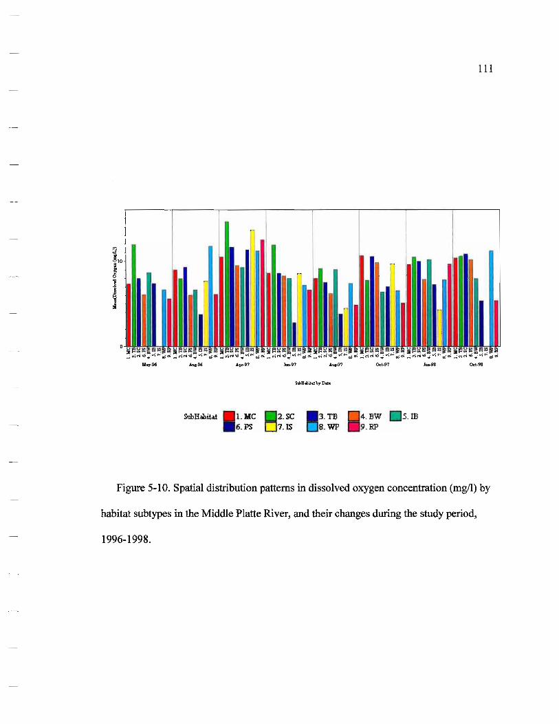
SubHabit.t 11. MC 6.PS
SC 1. IS
3.TB WP
BW .RP
IB
111
Figure 5-10. Spatial distribution patterns in dissolved oxygen concentration (mgll) by
habitat subtypes in the Middle Platte River, and their changes during the study period,
1996-1998.
112
5.1.4 Specific conductance
Conductivity is a measure of electrical conductance of water and is an approximate
indicator of total dissolved ions (Allan 1995). Because conductivity is highly temperature
dependent, a correction for this variable must be made to a standard temperature of 25 0 C.
In surface water at all sites in the Middle Platte River, mean specific conductance was
989.2 Ils/cm during the study period (n = 430). Variation in conductance was higher in
backwaters and sloughs than in the main and side channels (Table 5-2). ANOVA (F (8,
107.5) = 7.74, P < 0.0001), and MCA analyses revealed significant differences in the mean
specific conductance between lentic habitats and lotic habitats. Mean specific
conductance ranged from 930 Ils/cm in main channels to 1107 Ils/cm in wet meadow
sloughs (Table 5-2, Figure 5-11). There was no significant difference in mean specific
conductance between side and main channels.
Seasonal changes in mean specific conductance for the entire river landscape were not
significant (ANOVA: F (7, 165.9) = 2.03, P = 0.0542). Most of the higher specific
conductance values were observed during dryer periods in late summer and fall , and when
surface water was shallow in lentic habitats (Figure 5-13). The mean specific conductance
was relatively lower in early summer, and higher in late summer and fall (Table 5-1 ,
Figure 5-12).
At the habitat scale, seasonal variation in specific conductance within each of the
habitat types had clear spatial patterns (Figure 5-13). Variation was greater in backwater
113
and wet meadow slough habitats than in main channel and side-channel habitats. In lentic
habitats, surface water conductivity was higher in summer, with the maximum values in
August. In contrast, it was lowest in spring, with the minimum value in April 1997
(Figure 5-13, 5-14).
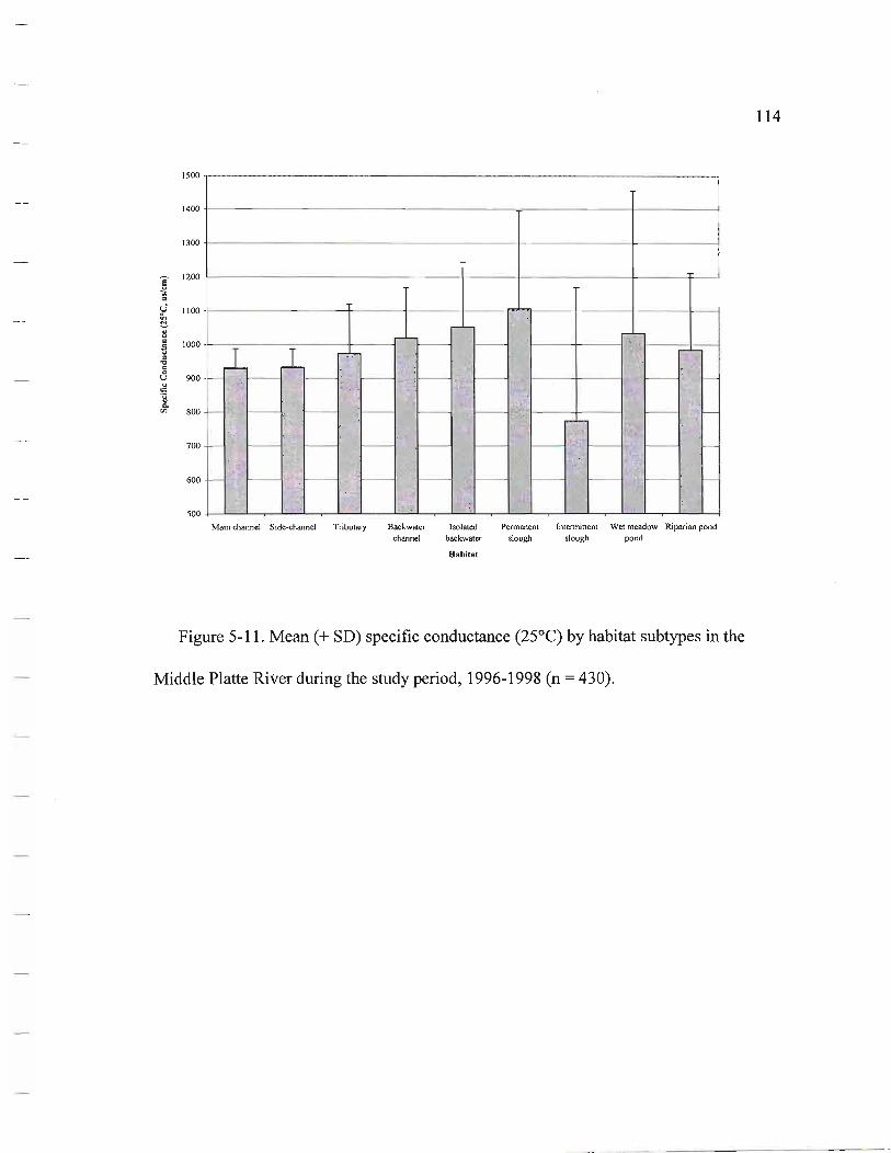
114
1500
1400
1300
E 1200
~ = ~ 11 00
C 1J = 1000 ~
1:i = '0 = C> U 900 " "" .~
"" '" 800
700
600
500
Main channel Side-channel Tributary Backwater Isolated Permanent Intermittent Wet meadow Riparian pond channel backwater slough slough pond
Habitat
Figure 5-11. Mean (+ SD) specific conductance (25°C) by habitat subtypes in the
Middle Platte River during the study period, 1996-1998 (n = 430).

1400 y-- ------ ---- - ----- - - --- ------_
1300 -j-------- --- --- - - -+- - --- - - - ---+---I
1200 -j--------=- - ------ - - -+- ----I-- - - - ---+---I
E 1I00 +-----_+---4----~--_+---+_------_+-~ ~ = U lh ~ 1000 +--f-----l----4----~-_II;» :m--___l ~ = ~ = ." a 900
800
700
May-96 Aug-96 Apr-97 Jun-97 Aug-97
Date
Ocl-97 Jun-98 Nov-98
Figure 5-12. Seasonal change in mean (+ SD) specific conductance (25°C) in the
Middle Platte River during the study period, 1996-1998 (n =430).
115

116
I.JolC 3. TB 2. SC 6. PS 4. BW S. IB 7. IS 8. WP 9. RP
0 ... by Sd!lUI>iUt
Date I May-96 Aut;-96 lm-97 A1l(-97 Oct-97 Jun-98
Figure 5-13. Changes in mean specific conductance (25°C) within habitat subtypes in
the Middle Platte River, 1996-1998.

118
5.1.5 Salinity
Salinity, another indicator for total dissolved salts, showed the same trends as specific
conductance. In the river floodplain, mean salinity of surface water was 0.5 ppt (n = 395)
during the study period, with little change from spring to fall, and only slight differences
among habitats (Table 5-2, Figure 5-15). Salinity in main channels and side-channels was
0.4-0.5 ppt, while in other lentic environments it was generally?: 0.5 ppt. ANOVA (F (8,
99.62) = 7.37, P < 0.0001), and MCA analyses revealed significant differences in mean
salinity (ppt) between backwater and slough and main and side channel, but no significant
difference between main channel and side channel habitats. Some sites where salinity was
as high as 0.8-1.1 ppt, were consistent with those with high conductivity (refer to Table 5-
2, Figure 5-11).
Seasonal changes in mean salinity in the river valley were small (Table 5-1 ,
Figure 5-16) although an ANOV A (F (6, \62.9) = 3.72, P = 0.0017) suggested that there
were significant differences between summer and fall. Comparing mean salinity among
the four habitat types at the habitat scale, seasonal fluctuations in mean salinity in each of
the four habitat types were significant for lentic habitats (Figure 5-17). Two distribution
patterns in surface water mean salinity were found (Figure 5-18): a relatively flat spring
pattern versus an abruptly changed summer-fall season pattern, reflecting a significant
seasonal fluctuation in backwater and wet meadow habitats. These distribution patterns
were very similar to patterns of specific conductance (Figure 5-14).
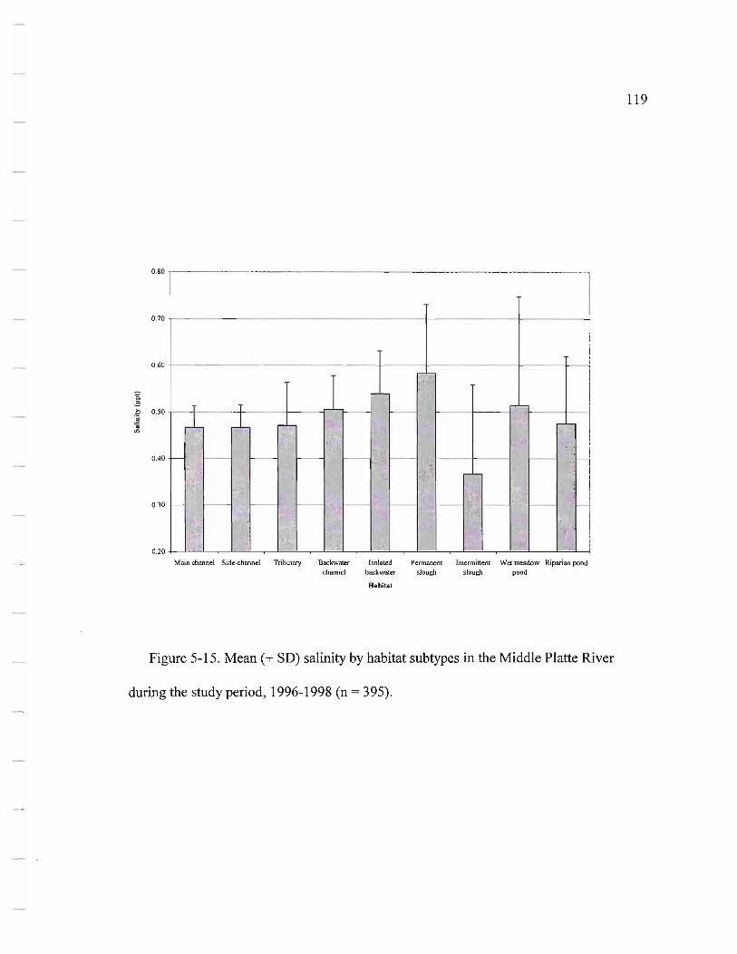
119
0.80 .-------.-.-.-.. -.-------------------- ... ---.. --..... --.-----.-..... -
0.70 -1-- --- ---- - - - - --------+-------- 1- - - - ----1
0.60
~ 5 :c 0.50 -'c ;; '"
0.40
Main channel Side-channel Tributary Backwater Isolated Permanent Intennittent Wet meadow Riparian pond channel backwater slough slough pond
nabitat
Figure 5-15. Mean (+ SD) salinity by habitat subtypes in the Middle Platte River
during the study period, 1996-1998 (n = 395).
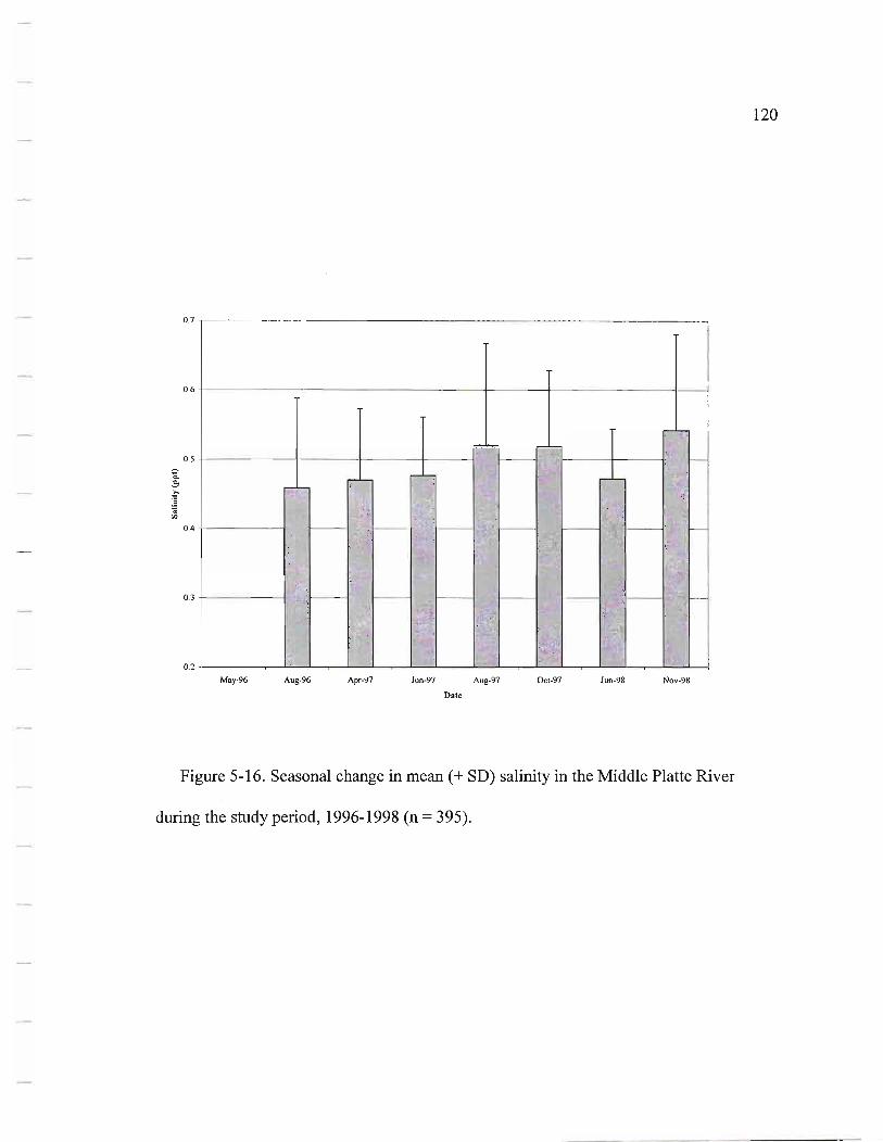
120
0.7 T--.···-·-··.··············------------·-·.·-··.·.···· .. -.-.--........... ---.-.. -..... - .. -.---.. ----..... .....,
0.6 f-------- - - --- - - - -f-- - - +-- --- - - - I-----!
0.5
~ -= ~ :5 ... '"
0.4
0.3 +-- ---
May-96 AuS-96 Apr-97 Jun-97 Aug-97 Ocl-97 Jun-98 NoY-98
Date
Figure 5-16. Seasonal change in mean (+ SD) salinity in the Middle Platte River
during the study period, 1996-1998 (n = 395).

0.9
I.KC J.TB 2.se
Date I MaY.96 Oct-97
6. PS 4. BW S. IB 7. /S B.WP 9. RP
Jun·97
Figure 5-17. Seasonal changes in mean salinity by habitat subtypes in the middle
Platte River, 1996-1998.
121

122
1.0,-----;-----,-------;--------;-----.------,-----,...------,
SubHabit~t 11. MC 6. PS
SC . IS
TB VIP
BW RP
IB
Figure 5-18. Spatial patterns of mean salinity by habitat subtypes and their seasonal
changes during the study period, 1996-1998.

123
5.2 Nutrients of surface water in riverine habitats
Nitrogen was analyzed as nitrate + nitrite (N03- + N02-), and ammonium (NH/).
Nitrite was not detected or was below the limitation of detection in most samples.
The mean N03-N + N02-N concentration (n= 381) was 0.76 (± 1.14) mg/L for the
study period. Ninety percent of the N03-N + N02-N values were below 2.35 mg/L, and
about 2% of the samples had levels greater than 5 mgIL. These relatively high values of
N03- + N02- were found in tributary type habitats (Table 5-3, Figure 5-19) that linked
with irrigation drainage ditches, or flow-through pastures. Higher nitrogen concentrations
in tributary streams suggested that dissolved N03-N + N02-N were released mainly from
agricultural runoff (irrigation drainage and grazing land surface and subsurface flow) . The
mean N03-N + N02-N concentration in the main channel was 1.07 (± 0.64) mg/L, while
some sites with adjacent cropland had 2-3 mgIL nitrate + nitrite. Most of the backwater
and wet meadow slough habitats had very low N03-N + N02-N concentrations (Table 5-
3, Figure 5-19). ANOVA (F (8, 100.43) = 58.0187, p< 0.0001) and MeA analyses
showed significant differences in mean N03-N + N02-N levels in surface water among
the habitat subtypes (Figure 5-19). Specifically, there were significant differences
between the lotic group (i.e. main channel and side-channel) and the lentic group (i.e.
remaining habitat subtypes except intermittent sloughs and wet meadow ponds).
Backwater, permanent slough, and riparian pond habitats had very low nitrogen

124
concentrations, while the tributary had a very high nitrogen concentration. Spatial
heterogeneity in N03-N + N02-N concentrations at the landscape scale was obvious and
constant through all seasons (Figure 5-20).
ANOVA (F (5, 152.8) = 10759, P = 0.3740, a = 0.05) indicated no significant difference
in mean concentrations ofN03-N + N02-N among seasons in the Middle Platte River
(Table 5-4, Figure 5-21). At the habitat level, however, the seasonal difference of the
mean concentrations ofN03-N + N02-N is noticeable for the types of main channel
(ANOVA, F (5, 9.719) = 7.58, p= 0.0038) and side-channel (ANOVA, F (5,6.2071 ) = 13.27, P
= 0.0030), (Figure 5-22). The higher seasonal variation in N03-N + N02-N levels
occurred in spring 1997 in the main channel, and in spring and summer 1997 in side
channel habitats. There were insufficient numbers of samples for statistical analysis on
isolated backwater, intermittent slough, and riparian pond habitats, because most of these
habitats were dry in summer.

Table 5-3. Spatial heterogeneity of nutrients and major dissolved ions (mean ± SD) in surface water of aquatic habitats in the Middle
Platte River during the study period, 1996-1998 (n = 381), summarized by aquatic habitat subtype.
Habitat ~-N N03-N+N02-N P04-P cr SO/- K+
n (mg/L) (mg/L) (mg/L) (mg/L) (mg/L) mg/L)
Main channel 89 0.02± 0.04 1.07 ± 0.64 0.03 ± 0.03 37.2 ± 7.7 266.7 ± 40.3 10.2 ± 1.1
(MC)
Side-channel (SC) 26 O.oI ± 0.02 0.79 ± 0.38 0.02± 0.02 36.1 ± 4.6 264.6 ± 21.1 10.6 ± 1.2
Tributary 43 0.09 ± 0.14 2.68 ± 1.88 0.1O±0.15 41.6 ± 13.1 234.5 ± 60.0 12.5 ± 2.0
(TB)
Connected 79 0.02 ± 0.06 0.29 ± 0.51 0.03 ± 0.09 38.3 ± 8.7 288.4 ± 85 .4 10.0±1.4
backwater (CB)
Disconnected 36 0.03 ± 0.09 0.06± 0.22 0.04 ± 0.04 39.9 ± 10.6 315.4± 117.1 10.2 ± 2.2
backwater (DB)
Permanent slough 47 0.03 ± 0.07 0.19±0.41 0.03 ± 0.03 38.4 ± 10.7 314.9± 100.3 7.9 ± 2.7
(PS)
Intermittent slough 12 0.03 ± 0.08 0.75 ± 1.18 0.22 ± 0.33 24.7± 17.2 158.4 ± 157.1 14.0 ± 2.9
(IS)
Wet meadow pond 28 0.08 ± 0.23 0.58 ± 1.10 0.12 ± 0.21 38.5 ± 18.6 330.4 ± 184.4 10.6 ± 3.4 (WP)
Riparian pond 21 0.03 ± 0.07 0.01 ± 0.01 0.03 ± 0.08 40.6 ± 12.3 255.8 ± 77.6 10.0 ± 2.6
(RP)
Na+ Ca2+ (mg/L) (mg/L)
58 .2 ± 16.7 47.1 ± 7.1
60.4 ± 17.7 49.9± 9.3
56.6 ± 16.2 56.4± 12.9
61.7± 15.9 57.5 ± 11.7
62.5 ± 19.9 59.5 ± 13 .6
67.5 ± 19.9 62.2 ± 14.4
29.6 ± 21.4 39.5 ± 15.4
61.5 ± 25.2 57.0 ± 22.4
65.3 ± 22.0 59.6 ± 12.9
Mg2+ (mg/L)
20.5 ± 1.8
21.0 ± 1.6
21.7 ± 3.6
22.1 ± 2.8
22.8 ± 4.1
22.1±3.9
14.6 ± 7.6
22.4± 6.6
21.7 ± 4.5
....... tv VI

Table 5-4. Temporal changes in nutrients and major dissolved ions (mean ± SD) in surface water of aquatic habitats in the Middle
Platte River during the study period, 1996-1998 (n = 381).
Date ~-N N03-N+N02-N P04-P CI- SOl" K+ Na+ Ca2+ MgH
n (mg/L) (mg/L) (mg/L) (mglL) (mg/L) mglL) (mg/L) (mglL) (mglL)
May-96 33 0.02 ± 0.07 0.62 ± 1.33 0.07 ± 0.15 24.4± 7.5 206.7 ± 65.6 9.5 ± 2.8 68.3 ± 18.8 62.8 ± 11.7 19.8 ± 4.6
Aug-96 71 0.03 ± 0.11 0.63 ± 1.12 0.09 ± 0.11 29.5 ± 7.8 229.9 ± 95.8 10.2 ± 2.7 66.4 ± 19.8 56.5 ± 18.6 21.0 ± 4.8
Apr-97 62 0.02 ± 0.04 1.12 ± 1.49 0.01 ± 0.03 46.1 ± 7.8 302.6 ± 65.9 10.2 ± 2.6 32.2 ±2.6 46.3 ± 5.6 21.2± 1.9
Jun-97 72 0.09 ± 0.17 0.68 ± 0.97 0.01 ± 0.03 40.2± 8.6 284.8 ± 50.2 9.9 ± 1.7 71.0 ± 8.3 52.6 ± 10.2 22.0 ± 2.5
Aug-97 71 0.03 ± 0.06 0.77 ± 0.85 0.09 ± 0.18 39.8 ± 9.8 323.7 ± 135.7 10.7 ± 2.4 55.4±17.8 62.2± 14.0 21.4 ± 5.0
Oct-97 72 0.00 ± 0.01 0.72 ± 1.11 0.03 ± 0.11 42.8 ± 9.7 290.5 ± 87.0 10.8 ± 2.0 68.4 ± 10.8 51.0 ± II. 7 22.2 ± 3.6
-tv 0'\

127

4.20 -1-----------+--------------------------1
3.60 -1- - - ---- --_1_----- -------- -------------1
3.00 +----------+- -------- -----------------1
.~ 2.40 -1---------1 ,;;1--- - - - --- - --- -------------1
i + " ~ i 1.80 +--- ------1
1.20 -l--f-----,~--lr 4W\'I_--------------I__--_I_-----__1
0.60
Main channel Side-channel Tributary Backwater Isolated Permanent Intermittent Wet meadow Riparian pond channel backwater slough slough pond
Habitat
Figure 5-19. Mean (+ SD) concentrations of nitrogen (N03-N + N02-N) by habitat
subtypes in the Middle Platte River during the study period, 1996-1997 (n = 381).
127

128
0.0
11.,.· 96 .\~.96 Apr.91 _91 .\"(-91 Oct·91
&i>-1ubiUI by Dolo
Sllb-habitu I I. MC .SC TB 4. BW .5.IB 6.PS . IS . VIP .RP
Figure 5-20. Spatial patterns of mean (+ SD) nitrogen (N03-N + N02-N) across
habitat subtypes, and their seasonal changes during the study period, 1996-1997.
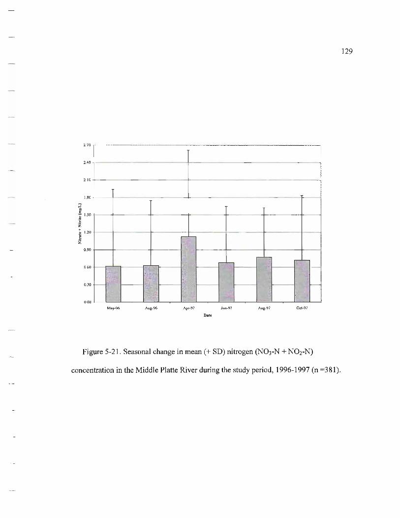
2.70 , ... ---.---..•. - ..•........•.••........ ----•.. - --.. - -----------------------.......... ~
2.40 +-- --- - --- - - - -+-- - ----- --- -------1
2.10 +--- --- --- ---+-------------------1
1.80 -J-- -+------ ----J---- --------- --.::r----1
~ ~ 1.50 t---1-- - ---I----- t--------1I------1---- - -I-------4 .~
b Z t 1.20 t-- -1-- - - - -I-- ---+---- ----11--- - - -1-- - - - -I--- ----4 ~ Z
0.90 -/-- --+---- +-- - -1
0.60 .I-----c:;;:;'-__ ----li
0.30
May-96 A ug-96 Apr-97 Jun-97 A ug-97 Oct-97
Date
Figure 5-21. Seasonal change in mean (+ SD) nitrogen (N03-N + N02-N)
concentration in the Middle Platte River during the study period, 1996-1997 (n =381).
129

Date I MaY-96 Oct-91
Aug-96 • Apr-97
l30
Jun-97
Figure 5-22 Seasonal changes in mean nitrogen (N03-N + N02-N) concentration in
each of the habitat subtypes in the Middle Platte River, 1996-1997.
- -- - - - ----
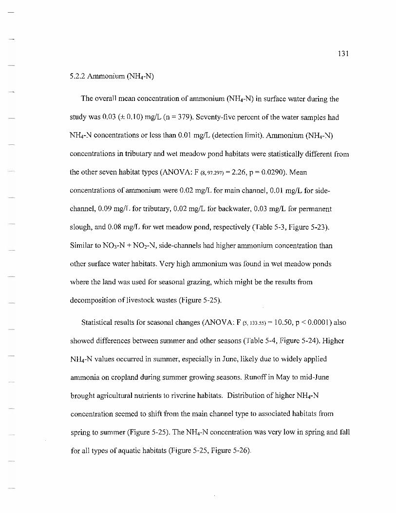
131
5.2.2 Ammonium (NH4-N)
The overall mean concentration of ammonium (NH4-N) in surface water during the
study was 0.03 (± 0.10) mg/L (n = 379). Seventy-five percent of the water samples had
NH4-N concentrations or less than 0.01 mg/L (detection limit). Ammonium (NH4-N)
concentrations in tributary and wet meadow pond habitats were statistically different from
the other seven habitat types (ANOY A: F (8, 97.297) = 2.26, P = 0.0290). Mean
concentrations of ammonium were 0.02 mg/L for main channel, 0.01 mg/L for side
channel, 0.09 mg/L for tributary, 0.02 mg/L for backwater, 0.03 mg/L for permanent
slough, and 0.08 mg/L for wet meadow pond, respectively (Table 5-3, Figure 5-23).
Similar to N03-N + N02-N, side-channels had higher ammonium concentration than
other surface water habitats. Yery high ammonium was found in wet meadow ponds
where the land was used for seasonal grazing, which might be the results from
decomposition of livestock wastes (Figure 5-25).
Statistical results for seasonal changes (ANOYA: F (5, 133.55) = 10.50, P < 0.0001) also
showed differences between summer and other seasons (Table 5-4, Figure 5-24). Higher
NH4-N values occurred in summer, especially in June, likely due to widely applied
ammonia on cropland during summer growing seasons. Runoff in May to mid-June
brought agricultural nutrients to riverine habitats. Distribution of higher NH4-N
concentration seemed to shift from the main channel type to associated habitats from
spring to summer (Figure 5-25). The NH4-N concentration was very low in spring and fall
for all types of aquatic habitats (Figure 5-25, Figure 5-26).
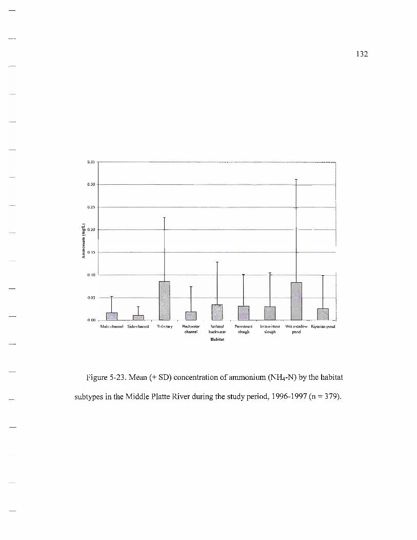
0.35 .,..----------------------------------~
0.30 ~----------------------------___11___----____'
0.25 +-- - - - - - --- - --- - - - ------ - --- - -11---- -----1
~ lO.20
~ ·c o ~ 0.15 +-- - -------4-------------- --- - ___11___- ---____' «
0.10 +--- - - -----4---------1----..,---- +--- ___11___- - --.--1
0.05 -1- ----'lF----- --- 1-- - +--- --I------f- ---+---r ':;"I------I------l
Main channel Side-channel Tributary Backwater Isolated Permanent lntermittent Wet meadow Riparian pond channel backwater slough slough pond
Habitat
Figure 5-23. Mean (+ SD) concentration of ammonium (NR.-N) by the habitat
subtypes in the Middle Platte River during the study period, 1996-1997 (n = 379).
132
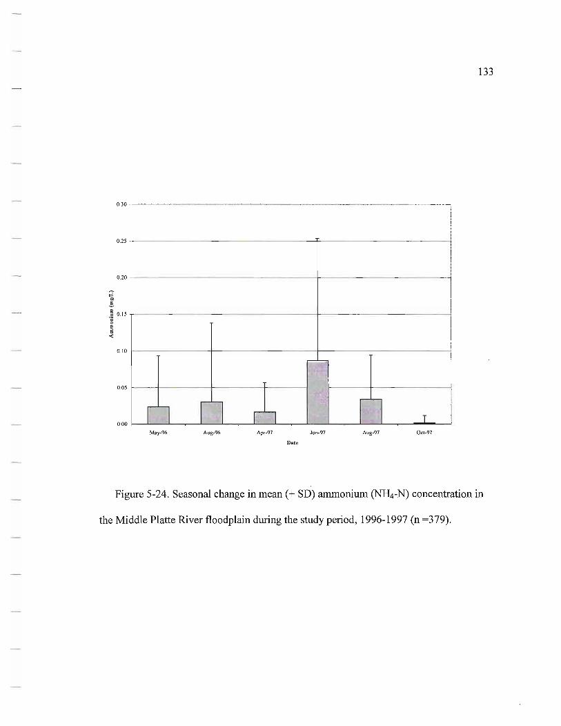
0.30 ,-.. ----...... -.---.. --.... --... -.---................ - ... -.-.-...................... --.. --------... - ...... ---...... -................... -... ---.......... -.---......... ~
0.25 -j--------- ---- - - - ........:f--- - - --- - - - - -'
0.20 -j--------- ---- - - ---I-- - - -----------1
; 0.15 -j------------- - - ---I--- ------ - - ----1 .. o E E
...:
O.IO -f---- - - ----I-----------J---------------1
0.05 ~---+----_I-----+_--_l
May-96 Aug-96 Apr-97 Jun-97 Aug-97 Oct-97
Date
133
Figure 5-24. Seasonal change in mean (+ SD) ammonium (NH4-N) concentration in
the Middle Platte River floodplain during the study period, 1996-1997 (n =379).

0.40
D~e I M.a.Y-96 Oct-97
Aug-96 • Apr-97
134
Jan-97
Figure 5-25. Changes of mean ammonium CNH4-N) concentration in habitat subtypes
in the Middle Platte River, 1996-1997.

S,m-habitat . 1. MC . O. PS
2.SC . IS
3.TB D 4.BW 8 . WP . 9 . RP
135
5. IB
Figure 5-26. Spatial patterns of mean ammonium CNH4-N) concentration in the habitat
subtypes in the Middle Platte River, and their seasonal changes during the study period,
1996-1997.
136
5.2.3 Phosphorus (P04-P)
Most dissolved phosphorus concentrations (P04-P) in the water samples were
approximately 0.003 mg/L (the detection limit). Mean phosphorus concentrations of all
water samples (n = 381) was 0.05 (± 0.12) mg/L. Difference of mean phosphorus
concentration among the habitat subtypes is significant (ANOYA, F (8, 96.641) = 2.76, P =
0.0087). Tributary, wet meadow pond, and intermittent slough habitats had higher mean
concentrations (~0.10 mg/L) while phosphorus levels in other aquatic habitats were all
lower than 0.04 mg/L (Table 5-3, Figure 5-27). The seasonal difference was also
significant statistically (ANOYA, F (5, 145.34) =12.8, p< 0.0001) at the whole river
ecosystem scale (Table 5-4, Figure 5-28). Higher phosphorus concentrations in surface
water were detected mainly in samples collected during summer. These samples (> 0.20
mgIL) were not collected from the main channel, and only a few from grazed wet
meadow habitats (Figure 5-29). The high phosphorus concentration values were likely
related to agricultural activities on land adjacent to side channels, and associated to
backwater areas. Seasonal variation in phosphorus concentrations was dramatic in the
main channel and side-channel habitats. However, it was very low in both the backwater
and wet meadow habitats. This temporal pattern of phosphorus variation across the
aquatic habitat types was seen in all of the summers sampled. Phosphorus remained very
low during other seasons, and there was no significant difference among these habitat
types (Figure 5-29, 5-30).

0.60
0.55
0.50
0.45
0.40
~ 0.35 !,
e 0.30 o .c c.. ~ 0.25 =-
0.20
0. 15
0.10
0.05
0.00
137
;
."<to ;''Ii
iij+;i~1 r-'-
i\)
T I ~~: T T ' .~
~ ~ 'I'd ~ ~ ~ ~0~1 I~~~ ~ Main channel S ide-channel Tributary Backwater Isolated Permanent Intennittent Wet meadow Riparian pond
channel backwater slough slough pond
Habitat
Figure 5-27. Mean (+ SD) phosphorus concentration by habitat subtypes in the Middle
Platte River during the study period, 1996-1997 (n = 381).
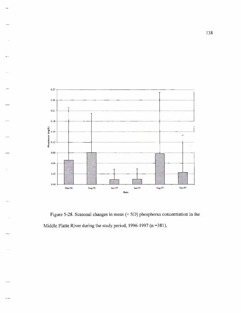
138
0.27
0.24
0.21
0.18
~ .. ..§, 0.15
~ 0 .c ~ 0.12
.c ~
0.09
0.06
0.Q3
0.00
May-96 Aug-96 Apr-97 Jun-97 Aug-97 Ocl-97
Date
Figure 5-28. Seasonal changes in mean (+ SD) phosphorus concentration in the
Middle Platte River during the study period, 1996-1997 (n =381).
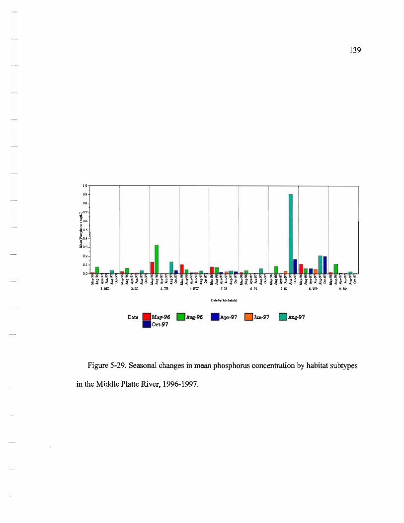
139
1.0,--------;----;------,-------,----------;----;------,-----,----------,
09
0.8
O.~
0.1
I.MC 2.SC 3. TB 4. BW s.m 6 . PS 1 . IS 8. WP 9.RP
. Apr-97 o Jun-97 Aug-97
Figure 5~29. Seasonal changes in mean phosphorus concentration by habitat subtypes
in the Middle Platte River, 1996~1997.

140
1.0,-------.-------;---------,-----------,..--------;--------,
0.9
0_8
0.2
S1.lb-habitat 11. MC 6. PS
Stlb-lutbitu 'by Due
.SC
. IS 5.IB
Figure 5-30. Spatial patterns of mean phosphorus concentration by habitat subtypes in
the Middle Platte River, and their seasonal changes during the study period, 1996-1997.

141
5.3 Major dissolved ions
5.3.1 Calcium (Ca)
The mean calcium concentration in surface water of the Middle Platte River was 54.6
(± 13.8) mg/L during the study seasons (n = 377). The spatial distribution of calcium was
significantly different (ANOYA: F (8,94.162) = 13.71 , p< 0.0001), with a trend for a
decrease in concentration along the gradient: permanent slough or pond --> backwater -->
side-channel--> main channel. The main channel had the lowest calcium content (Table
5-3, Figure 5-31). Most of calcium concentrations in samples from main channels were
lower than the mean level of calcium for the entire river floodplain. Calcium
concentration was higher during summer and lower in fall and spring, except in spring
1996 (Table 5-4, Figure 5-32) (ANOYA: F (5, 150.5) = 25.38, p< 0.000l). Figure 5-33
shows seasonal changes in mean calcium levels within the aquatic habitat subtypes.
Multiple comparison analysis showed that the entire habitat subtypes except intermittent
sloughs and wet meadow ponds had significant seasonal differences in calcium
concentration. Calcium levels in the main and side-channels were relatively less variable
than in riverine habitats. Figure 5-34 illustrates the temporal change in the calcium spatial
distribution pattern among habitat types. It appears similar to the pattern described above,
except that in late spring 1996. Trends in calcium decline were the same, but the slopes of
the gradients were less in spring and fall, and abrupt in surru:n.ers. Multiple comparison
analysis showed that there was no significant difference in mean calcium concentration in
142
spring 1996 and 1997. The distribution of calcium in late May 1996 was likely influenced .
by a flood event after several days of heavy rain (samples were collected after the flood).
The highest calcium concentrations were found in wet meadow sloughs. For example,
water samples collected from two wet meadow sloughs and one shallow water pond on
Mormon Island Crane Meadow exhibited calcium levels of 50-67 mg/L in late May 1996,
which increased to 124-157 mg/L in August 1996. That is, the calcium concentration
increased almost three times within three months. In spring 1997, water samples from the
same sites had calcium levels down to 45.2-55.2 mg/L. This decline was explained by
detailed field surveys of soil and vegetation, and land-use history gathered from local
landowners. In November 1995 and April 1996, landowners burned the wet meadow and
grassland plots to maintain native wet meadow species. These burned plots were
upstream of the wet meadow sloughs and the pond. Cations were released from the
burned plant ash and concentrated in the sloughs and pond by surface runoff. Intermittent
sloughs had the lowest mean calcium concentration.
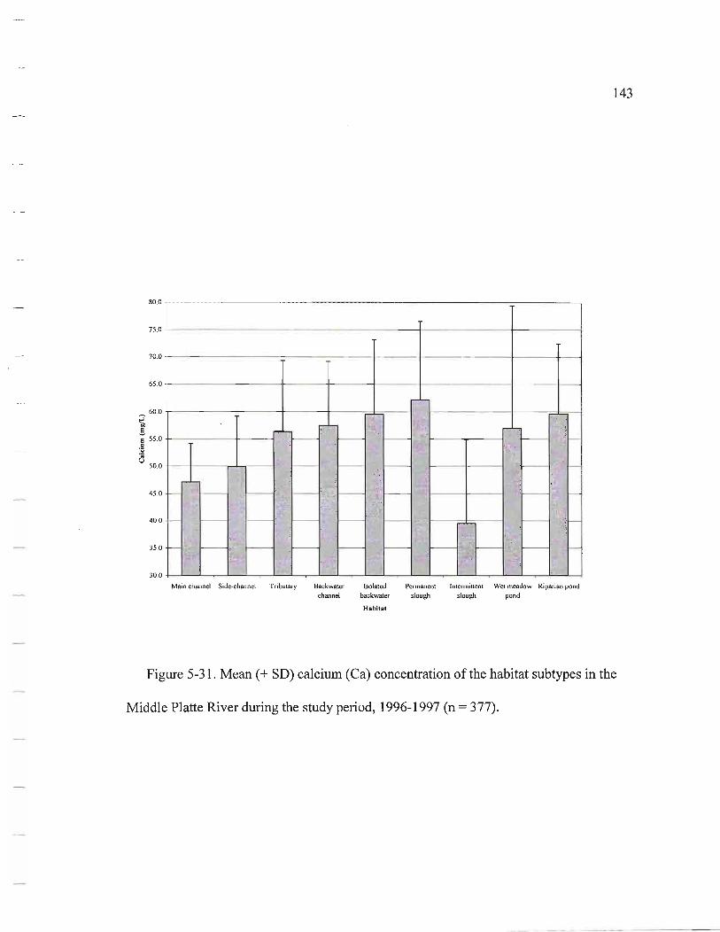
80.0 ,....-------------------------------------,
75 . 0 +----------------------~-------_+-----~
70.0 +-------------------+----~-------_+---_I_-~
65 .0 +-----------\-----j-----+----~-------_+----I·-~
~ 60.0 +-- ----- ---+ ---+-- --;:±::;---I,
e '8 55 .0 +--- - --+ - - - 110:;;),1-- --1 = 'y
d 50.0 +--+----,.....L.,...------I." ..
45 .0
40.0
35.0
30.0 -l---'-'='--...,.--'--
Main channel Side-channel Tributary Backwater Isolated Permanent Intermittent Wet meadow Riparian pond channel backwater slough slough pond
Habitat
143
Figure 5-31. Mean (+ SD) calcium (Ca) concentration of the habitat subtypes in the
Middle Platte River during the study period, 1996-1997 (n = 377).

144
80.0
75 .0
70.0
65 .0
60.0
~ on e e 55.0
'b " u
50.0
45 .0
40.0
35.0
30.0
May-96 Aug-96 Apr-97 Jun-97 Aug-97 Ocl-97
Date
Figure 5-32 . Seasonal changes in mean (+ SD) calcium (Ca) concentration in the
Middle Platte River during the study period, 1996-1997 (n =377).

80
1.IIC 2.SC 3. TB 4. BW s.m 6. PS 7. IS 8. WP
DAt. by Stm-Nbit ... t
Date A1lg-97
Figure 5-33. Seasonal changes in mean calcium (Ca) concentration by habitat
subtypes in the Middle Platte River, 1996-1997.
145
9. RP
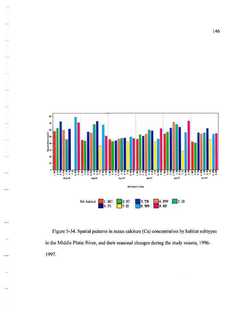
Sub-habitat I . MC . PS
Sd>-habiW by Date
2. SC 7. IS
3. TB 8. WP
.BW
.RP 5. IB
146
Figure 5-34. Spatial patterns in mean calcium (Ca) concentration by habitat subtypes
in the Middle Platte River, and their seasonal changes during the study season, 1996-
1997.

147
5.3.2 Magnesium (Mg)
Magnesium in surface water had a similar distribution pattern to that of calcium. The
mean magnesium level for all surface water samples (n = 381) collected from the river
and floodplain was 21.4 (± 3.9) mgIL during the study period. The spatial distribution of
magnesium in surface water followed the same trend as that of calcium (Table 5-3, Figure
5-35), but was less statistically significant than calcium (ANOV A: F (8,95.06) = 4.80, p<
0.0001). Intermittent sloughs had the lowest content of magnesium in water. Seasonal
changes in magnesium concentration were not significant (ANOVA: F (5, 150.98) = 2.41, P
= 0.0393) (Table 5-4, Figure 5-36). Temporal changes in magnesium levels within each
habitat type (Figure 5-37) and seasonal changes in the distribution pattern across habitat
types (Figure 5-38) were also less distinct than that of calcium. No significant fluctuation
except relatively low values in May 1996 was observed.

30.0 r-------------------------------------------------------------------__
28.0 +---------------------------------------------------------~--------~
26.0 +---------------------------------~------~--------------~----~~~
24.0 +------------------4-------4-------~------4_--------------~----~--~
:J 22.0 +---+-------f------4------;,......-.-.----I. ' <6 1-----=hr------"I'-----1 .. " 4 - -----1------1 .. ~ § 20.0 -'-_I N · · 1.---'5 C .. ~ 18.0
16.0
14.0
12.0
Main channel Side-channel Tributary Backwater Isolated Permanent Intermittent Wet meadow Riparian pond channel backwater slough slough pond
Habitat
148
Figure 5-35. Mean (+ SD) magnesium (Mg) concentration by habitat subtypes in the
Middle Platte River during the study period, 1996-1997 (n = 381).

149
27.0 ,--- --- - - - ___ ___ __________ ___ ---,
24.5 +-- ----,o-- --- --t-- - - - - - - - - r-- - --If--- - --t- ---l
22 .0 -j---+- - - ---+-- - --+-__ ----,.
17.0
14.5
12.0
May-96 Aug-96 Apr-97 Jun-97 Aug-97 Ocl-97
Date
Figure 5-36. Seasonal changes in mean (+ SD) magnesium (Mg) in the Middle Platte
River during the study period, 1996-1997 (n =381).

150
~.------,-------,------,------,------,-------~-----,------.------.
l.lte 2. SC
D~te
3. TB·
M~y-96
Oct.97
4. BW 5. m 6 . PS 1 . IS 8 . WP 9. RP
Date 'by Sab-habitat
Aug-96 • Apr-97 DJun-97
Figure 5-37. Seasonal changes in mean magnesium (Mg) concentration by habitat
subtypes in the Middle Platte River, 1996-1997.

151
~.----------.----------.---------~---------,----------,----------.
25
S'lb-habitaf I . MC 6.PS
. SC
. IS .TB D4.BW .WP . 9. RP
.IB
Figure 5-38. Spatial patterns in the mean magnesium (Mg) concentration by habitat
subtypes in the Middle Platte River, and their seasonal changes during the study period,
1996-1997.

152
5.3.3 Potassium (K)
Potassium concentrations in surface water of the middle Platte River varied a little
seasonally (ANOVA: F (5,151.96) = 2.42, P = 0.0381) (Table 5-4, Figure 5-39). The mean
potassium level of the whole surface water in the river and floodplains was 10.3 (± 2.4)
mg/L (n = 381) during study period. The potassium concentration differed significantly
(ANOVA: F (8, 94.38) = 13.15, p< 0.0001) across habitat types (Table 5-3, Figure 5-40):
Mean potassium concentrations in permanent wet meadow sloughs was the lowest: 7.7
mg/L; tributary and intermittent sloughs had higher concentrations at 12.5 and 14.0 mg/L,
respectively. Concentration in pond, backwater, and main channel habitats were around
10.0-10.5 mg/L (Table 5-3). Seasonal variations in potassium concentration were higher
in wet meadow sloughs and isolated water bodies than in other lotic and semi-Iotic
habitats (Figure 5-41). The pattern of potassium distribution across the aquatic habitats
was not significant seasonally; however the magnitude of the difference in mean
potassium levels appeared lower in lotic habitats and the fluctuation was larger in the
intermittent slough and wet meadow pond (Figure 5-42).
- -- - - - ----- - -------------------

153
13.3 , --.. -....... --.. - ..... - ...... -.............. ---..... - .... - .. --.-.. --.---.............. -.--.. --.... -.. -----.. --.--..... - .. -.--.-...... - .. ---.-.--.. ----... ,
12 .6 +---- - - - - - 1-- - - - - 1------ --- ---1-- - - - +----1
11.9 +----+-- - - -j-------I--- - - - -----+-----+------1
11.2 +---I-- ----+-------I--------I----- +--- - - - -I-----j
~ r 10.5
= . ~ = 9.8 +----1-----1 ~
9. 1
8.4
7.7
May-96 Aug-96 Apr-97 Jun-97 Aug-97 Oct-97
Date
Figure 5-39. Seasonal changes in mean (+ SD) potassium (K) concentration in the
Middle Platte River during the study period, 1996-1997 (n =381).
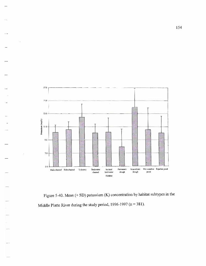
154
17.0 ,----___________________ -:;;-_______ ~
15 .0 i----- - --- - ---- --- - -----+ - - - --- ----J
13.0
~ ,§, 5 .~
11.0
S '" ...
9.0
7.0
5.0
Main channel Side-channel Tributary Backwater Isolated Permanent Intermittent Wet meadow Riparian pond channel baokwater slough slough pond
Habitat
Figure 5-40. Mean (+ SD) potassium (K) concentration by habitat subtypes in the
Middle Platte River during the study period, 1996-1997 (n = 381).

S1Jb..habitat I . MC . PS
2.SC . 3.TB . IS 8. WP
.BW
.RP 5. IB
156
Figure 5-42. Spatial patterns in mean potassium (K) concentration by habitat subtypes
in the Middle Platte River, and their seasonal changes during the study period, 1996-
1997.

157
5.3.4 Sodium (Na)
Sodium concentrations in surface waters varied only slightly in1996, but fluctuated
significantly in 1997 (ANOVA: F (5, 140.31) = 454.0, p< 0.0001). The mean of all samples
(n = 381) was 60.2 (± 19.4) mg/L. The lowest mean sodium concentration was in spring
1997 (32.2 mg/L), while in other seasons were from 55.4-71.0 mg/L (Table 5-4, Figure 5-
43). Samples collected during low flows (May and August, 1996 and August, 1997) had a
higher standard deviation in sodium concentration than those collected from high flows
(April, June, and October, 1997) (Table 5-4). Backwater, wet meadow, and other isolated
water bodies had somewhat higher sodium concentrations than main and side-channels
(ANOV A: F (8, 96.812) = 4.36, P = 0.0002) (Table 5-3, Figure 5-44), which might imply
effect of groundwater to these lentic habitats. Seasonal changes in mean sodium
concentration among aquatic habitat subtypes (Figure 5-45) were similar to potassium
fluctuations (Figure 5-41). There was no significant difference in the mean sodium
concentration, except in spring 1997. Seasonal distribution patterns in each of the habitat
subtypes were very similar except for ponds. Figure 5-46 illustrates spatial patterns of
mean sodium across aquatic habitats and their seasonal changes during the study period.
The distribution of sodium concentration across aquatic habitats was homogeneous.
--- -- -------------------------------------------------------------
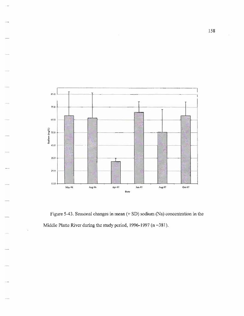
158
85 .0 +----+- - - - -t--------- - - - ----- -------1
75.0 +--- -+- ----t------ - - - - +-- -------- I----1
65.0
~ !: 55 .0
E = ;;; o
'" 45.0
35 .0
25 .0
15.0 -l----'----'-- r---'---'----.--"
May-96 Aug-96 Apr-97 Jun-97 Aug-97 Ocl-97
Date
Figure 5-43 . Seasonal changes in mean (+ SD) sodium (Na) concentration in the
Middle Platte River during the study period, 1996-1997 (n =381).

90.0 ,....-----------------------------------~
80.0 +------------------~---~-------_+---~·-~
70.0 -1-- -1-- - - -1-- --+ --- + - --+ ---+ --------+----+- ---1
~ 60.0 +-- +-----F:t-l---+-- - -l .. .§, E = ii J) 50.0
40.0
30.0 +----l %91',·1---
Main channel Side-channel Tributary Backwater Isolated Permanent Intermittent Wet meadow Riparian pond channel backwater slough slough pond
Habitat
Figure 5-44. Mean (+ SD) sodium (Na) concentration by habitat subtypes in the
Middle Platte River during the study period, 1996-1997 (n = 381).
159

100
90
l.lIe 2. SC 3. TB
Date I Ma.Y-96 Oct-97
4. BW
160
S.ffi 6. PS 7. 15 B. WP g. RP
Jun-97
Figure 5-45. Seasonal changes in mean sodium (Na) concentration by habitat subtypes
in the Middle Platte River, 1996-1997.

161
llO...--------r----------,~----___,_----____;_-----.,.._----_,
100
90
S1lb-habitat I . MC PS
2.SC 7. IS
TB . WP
BW .RP
5. IB
Figure 5-46. Spatial patterns in mean sodium. (Na) across habitat subtypes in the
Middle Platte River, and their seasonal changes during the study period, 1996-1997.
162
5.3.5 Chloride
The mean chloride concentration for all surface water samples collected from the river
and its floodplain was 38.2 (± 11.0) mg/L (n = 378) during the study period. Seasonal
variation in chloride (ANOVA: F (5, 156.39) = 55.04, p< 0.0001) was remarkable. Mean
chloride concentrations in 1997 were 30 to 50 % higher than those in 1996 (Table 5-4,
Figure 5-47), but still within normal levels compared with other reports for the same
reach ofthe river (Drever 1982; Engberg 1983; Frenzel et al. 1998). Mean chloride
concentration across habitat subtypes was very close, with no statistical differences found
(ANOV A: F (8, 90.624) = 1.96, P = 0.0603) (Table 5-3, Figure 5-48). There were significant
increases in chloride in both backwater and wet meadow habitats since summer 1996 and
through 1997 (Figure 5-49). The same increase occurred in main channels and side
channels, but a large (50 %) increase occurred in spring, 1997 then declined back to about
35-40 mg/L where it remained through the rest of 1997. Seasonal differences in the
distribution of chloride were not obvious (Figure 5-50). Statistical analysis showed that
there is no significant difference in chloride concentration among riverine habitats in
spring. Chloride concentrations in the intermittent slough fluctuated more than other
types in summer and fall. Overall, seasonal changes in the patterns of chloride
concentration across habitat types was not significant in the spring, but was significant in
the summer and fall. Permanent sloughs had slightly higher chloride levels, while
intermittent sloughs were usually lower than other habitat types.
- ---- ---- - -------------------------------------------------

163
55 .0 -,------.-----.------------.-.. -----.......... - .-.-.-------.------....... _
50.0 +-- - - - - --- - - - - 1- - - --- - --- - ---- -1-----'
45_0 -1--------- ----1;
~ 40.0 -1--- - ---------1
,§, u
~ o a 35.0 +------- -+-----1
30.0 -1-- --1-- - - - -+-- - --1
25 .0 +-- -+- --- 1
20.0 -1----"""-'-"'''''------,_-'-
May-96 Aug-96 Apr-97 Jun-97 Aug-97 Oct-97
Date
Figure 5-47. Seasonal changes in mean (+ SD) chloride in the Middle Platte River
during the study period, 1996-1997 (n =378).

55 .0 +-----------,=------ - - - - - - - - --- - - - -!------ ----<
50.0 -\-----------If----- - - - --'F- --- - - - - - - - -!--- ---I------<
45 .0 -I-- .,...----- --- --If--- - --I- - - --l-- - - -I-- - --- - - -!--- ---I------<
~ !. ~ 40.0 o
:2 U
35.0
30.0
25 .0
20.0
Main channel Side-channel Tributary Backwater Isolated Permanent Intermittent Wet meadow Riparian pond channel backwater slough slough pond
Habitat
164
Figure 5-48. Mean (+ SD) chloride concentration by habitat subtypes in the Middle
Platte River during the study period, 1996-1997 (n = 378).
_._------- - -_ ... -- - - _._-_._----

165
ro.------,------,------,------,------,------,------r------,-----~
so
10
1. Me l . SC 3. TB 4. BW 5. 1B 6. PS 1 .1S 8. WP 9. RP
Date Aug-96 • Apr-97 DJun-97 Aug-97
Figure 5-49. Seasonal changes in mean (+ SD) chloride by habitat subtypes in the
Middle Platte River, 1996-1997 (n=378).

so
Stlb-habitat 1. MC G]2. SC 6. PS D7.Is
.TB
. WP 4. BW
. RP 5. IB
166
Figure 5-50. Spatial patterns in mean chloride across habitat subtypes in the Middle
Platte River, and their seasonal changes during the study period, 1996-1997.

167
5.3.6 Sulfate
The mean sulfate concentration for all surface water samples collected from the river
and floodplains was 278.9 (± 97.0) mg/L (n = 379). Seasonal changes (ANOYA: F (5,
154.34) = 14.99, p< 0.0001) and spatial distribution of sulfate (ANOYA: F (8, 94.431) = 5.19,
p< 0.0001) were similar to those of chloride. The sulfate concentrations in 1997 were
higher than those in 1996 (Figure 5-51). Sulfate concentrations were 15-20 % different
between lotic and lentic habitats, with exception ofthe intermittent slough (Figure 5-52).
For all study sites in the Middle Platte River, there was a general trend for sulfate to vary
less in main channel and side-channel habitats, with broad ranges in other low flow or
static water habitats, especially during summer (Figure 5-53, Figure 5-54).
- - -- ~- -

480.0 -j-- ----- - - - ---- - - - - --- - - ----- -----l
430.0 -j------- - - --- ----- -----I---- - - - --i
380.0 +---c----------------------I-----~---i
~ 330.0 -j---- - - - --- - - +-- - - -----=l=-------- - -I-- - - - --1-- -----l !. ~
~ -; {/J 280.0 +--- - - - - - -1--- - --1
230.0 +---1-- - - ---,--'-..,--- --1
180.0
130.0 +----"''--=--r---'--'" May-96 Aug-96 Apr-97 Jun-97 Aug-97 Oct-97
Date
Figure 5-51. Seasonal changes in mean (+ SD) sulfate in the Middle Platte River
during the study period, 1996-1997 (n =379).
168

550.0 .r------------------------------------~
500.0 -1-------- --------- --------------+-- - ----1
450.04- ------------------- - - - - - --- - - -1-- - - ---1
400.0 -1----- - --------- - ---+-- ---+---- ----+------ -1
~ 350.0 -1-- - - - - - ---- ---+-- ---+-- ---+- -------+-- - - - --1 -! :!
~ 300,0 -1--+-- --- - ----- - +-- - ---1 '"
250.0
200.0
150.0
100.0 .I----'-'-''"'-"''''---~-
Main channel Sidc:-channcl Tributary Backwater channel
Isolated backwater
Habitat
Permanent slough
Intermittent Wet meadow Riparian pond slough pond
Figure 5-52. Mean (+ SD) sulfate concentrations by habitat subtypes in the Middle
Platte River during the study period, 1996-1997 (n = 379).
169

170
400
I./ilC 2. SC 3.TH 4. BW S. IB 6. PS 7. 15 8. WP 9.RP
Da.te Au;-96 • Apr-91 DJun-91 Au;-91
Figure 5-53. Seasonal changes in mean sulfate concentration within habitat subtypes
in the Middle Platte River, 1996-1997 (n = 379).

171
~r-----------~--------~-----------.-----------.----------'-----------.
400
100
1Iq-96
Sub-habitat I . MC PS
Apr-97
2.SC 7. IS
.TB
. WP BW
. RP 5.IB
0..-97
Figure 5-54. Spatial patterns in mean sulfate concentration across habitat subtypes in
the Middle Platte River, and their seasonal changes during the study period, 1996-1997 (n
= 379).

172
5.4 Trace elements
Trace elements, especially arsenic, cadmium, lead, selenium, and zinc are
environmentally important because of their potential toxicity in small quantities both to
ecosystems and humans. Table 5-5 and 5-6 summarize the chemical analysis results for
the sixteen trace constituents in surface water samples from the Middle Platte River and
its floodplain. Some of the elements, such as Bi, Co, and Pb were in relatively low «
0.05 %) concentrations, or below detection limits. Table 5-5 summarizes the statistical
results for the four main habitat types. The results showed no spatial heterogeneity of the
trace elements in surface waters except iron and manganese, which were extremely high
in backwater and wet meadow slough types (Table 5-5). These higher values were found
mainly in summer 1996 (Table 5-6). Table 6-8 compares the results of trace element
analysis (excluding bismuth and titanium) with those from USGS reports for three stream
gauging stations along the Middle Platte River during 1981-1990 (Boohar et al. 1996,
1997, 1998; Frenzel et al. 1998). Overall, most of the trace elements had similar ranges as
in the USGS data, except manganese and zinc. Zinc concentrations were about two-fold
higher in the present study. Manganese levels were more than ten-fold higher than the
USGS figures. There was some concern that the higher concentrations of iron and
manganese found in most backwater habitats might be related to hunting activities, since
there were many spent shells evident in backwater bodies. Backwater sites are habitat for
white-tail deer, ducks, turkeys, etc.

173
Table 5-5. Spatial change in trace element concentrations (~gIL) summarized by the main
aquatic habitats in the Middle Platte River during the study period, 1996-1997.
Element Statistic Main Channel Side Channel Backwater Slough
n 84 62 142 37
Al Mean 11.5 12.3 10.6 9.5
Std. Dev. 6.1 13.2 4.8 2.3
Max. 50.0 110.0 30.0 10.0
n 84 62 142 37
As Mean 4.0 3.0 2.5 1.5
Std. Dev. 0.6 1.6 1.2 0.6
Max. 5.5 5.5 7.3 3.4
n 84 62 142 37
B Mean 103.4 98.3 106.6 79.7
Std. Dev. 22.9 23.3 35.7 31.3
Max. 134.0 139.0 256.0 223 .0
n 69 54 117 26
Bi Mean 0.1 0.2 0.2 0.1
Std. Dev. 0.4 0.4 0.5 0.2
Max. 2.1 1.9 3.0 0.9
n 84 62 142 37
Cd Mean 0.0 0.0 0.0 0.0
Std. Dev. 0.2 0.1 0.1 0.0
Max. 1.5 0.2 0.3 0.2
n 84 62 142 37
Co Mean 0.2 0.3 0.4 0.4
Std. Dev. 0.1 0.1 0.3 0.2
Max. 0.7 0.9 1.6 0.8
n 84 62 142 37
Cr Mean 1.0 1.1 1.5 1.6
Std. Dev. 1.1 1.5 1.4 1.7
Max. 4.0 6.0 6.0 6.0
n 84 62 142 37
Cu Mean 2.0 2.3 2.1 2.9
Std. Dev. 0.6 2.5 1.9 3.3
Max. 4.7 19.7 15.4 18.5

174
Table 5-5. (Continued) Spatial heterogeneity in trace element concentrations (llglL) summarized by main aquatic habitats the Middle Platte River during the study period, 1996-1997.
Element Statistic Main Channel Side Channel Backwater Slough
n 84 62 142 37
Fe Mean 4.2 8.7 10.9 31.4
Std. Dey. 11.2 15.8 34.3 57.8
Max. 70.0 80.0 340.0 330.0
n 84 62 142 37
Mn Mean 2.1 25.6 199.7 80.3
Std. Dey. 4.9 77.0 372.7 128.7
Max. 34.0 474.0 2338.0 670.0
n 84 62 142 37
Mo Mean 4.9 6.2 5.9 3.6
Std . Dey. 0.7 1.5 4.0 1.5
Max. 6.3 9.2 25.9 6.1
n 84 62 142 37
Ni Mean 1.8 2.1 3.6 2.4
Std. Dey. 0.4 0.8 3.5 0.7
Max. 3.6 5.8 38.9 4.6
n 84 62 142 37
Pb Mean 0.0 0.0 0.0 0.1
Std. Dey. 0.0 0.1 0.1 0.4
Max. 0.1 0.2 0.7 2.4
n 84 62 142 37
Ti Mean 4.3 5.2 6.1 10.2
Std. Dey. 1.6 7.8 14.0 23.1
Max. 7.0 65.0 157.0 125.0
n 84 62 142 37
V Mean 7.0 5.7 2.8 1.5
Std. Dey. 1.0 1.8 1.9 1.2
Max. 9.0 10.4 8.5 4.1
n 84 62 142 37
Zn Mean 42.8 34.9 38.3 27.2
Std. Dey. 57.9 30.7 92.3 32.1
Max. 444.7 160.7 1038.0 186.0

175
Table 5-6. Seasonal change in trace element concentrations (1lg!L) in the Middle Platte
River floodplain aquatic habitats during the study period, 1996-1997.
Element Statistic May-96 Aug-96 Apr-97 Jun-97 Aug-97 Oct-97
n 30 59 52 62 60 62
Al Mean 11.7 10.7 14.0 12.7 9.2 8.7
Std. Dey. 7.5 2.5 14.3 5.8 3.3 4.2
Max. 50.0 20.0 110.0 40.0 20.0 20.0
n 30 59 52 62 60 62
As Mean 2.4 3.1 2.2 3.0 3.6 2 .7
Std. Dey. 1.1 1.4 1.5 1.2 1.2 1.1
Max. 7.3 5.5 4.8 4.8 5.9 4.5
n 30 59 52 62 60 62
B Mean 90.4 65 .5 96.0 103.6 130.3 113.9
Std . Dey. 24.1 12.6 21.5 19.8 38.1 14.9
Max. 139.0 98.0 121.0 171.0 256.0 139.0
n 30 0 52 62 60 62
Bi Mean 0.1 0.2 0.3 0.2 0.0
Std. Dey. 0.2 0.4 0.5 0.5 0.1
Max. 0.9 1.9 2 .0 3.0 0.6
n 30 59 52 62 60 62
Cd Mean 0.0 0.0 0.1 0.0 0.0 0.0
Std. Dey. 0.0 0.0 0.1 0.0 0.1 0 .2
Max. 0.0 0.1 0.2 0.1 0.3 1.5
n 30 59 52 62 60 62
Co Mean 0.5 0.3 0.2 0.3 0.4 0.3
Std. Dey. 0.2 0 .2 0.1 0.2 0.2 0 .2
Max. 1.1 1.1 0.4 0.8 1.6 1.3
n 30 59 52 62 60 62
Cr Mean 3.8 1.6 0.6 0.8 1.2 0.9
Std. Dey. 1.5 0.6 0.6 1.0 1.8 1.0
Max. 6.0 3.0 2.0 3.0 6.0 3.0
n 30 59 52 62 60 62
Cu Mean 6.5 2.0 1.7 1.7 2.0 1.6
Std. Dey. 4.6 0.5 0.4 0.5 0.7 0.4
Max. 19.7 3.0 2.7 4.2 4.7 3.8

176
Table 5-6. (Continue) Seasonal change in trace element concentrations ()!g/L) in the
Middle Platte River floodplain aquatic habitats during the study period, 1996-1997.
Element Statistic May-96 Aug-96 Apr-97 Jun-97 Aug-97 Oct-97
n 30 59 52 62 60 62
Fe Mean 56.7 13.4 2.7 7.1 6.0 2.7
Std. Dey. 58.7 42.9 8.0 24.7 9.6 9.8
Max. 340.0 330.0 40.0 180.0 40.0 60.0
n 30 59 52 62 60 62
Mn Mean 250.8 246.6 12.0 48.9 63.3 57.5
Std. Dey. 244.8 469.5 31.2 151.9 214.2 168.3
Max. 761.0 2338.0 144.0 700.0 1105.0 907.0
n 30 59 52 62 60 62
Mo Mean 5.0 4.4 4.3 5.1 8.5 5.0
Std. Dey. 1.8 1.4 1.5 1.4 5.0 1.6
Max. 9.2 8.9 7.9 7.9 25.9 9.2
n 30 59 52 62 60 62
Ni Mean 3.6 2.4 2.1 2.4 3.1 2.8
Std. Dey. 1.2 1.2 0.9 1.2 1.8 4.9
Max. 5.9 8.9 5.4 7.2 9.3 38.9
n 30 59 52 62 60 62
Pb Mean 0.2 0.1 0.0 0.0 0.0 0.0
Std. Dey. 0.4 0.0 0.0 0. 1 0.0 0.1
Max. 2.4 0.2 0.1 0.7 0.2 0.3
n 30 59 52 62 60 62
Ti Mean 13.7 3.9 5.4 4.4 6.3 5.7
Std. Dey. 36.8 12.6 1.3 0.7 2.6 2.5
Max. 157.0 76.0 9.0 6.0 20.0 24.0
n 30 59 52 62 60 62
V Mean 2.2 4.2 4.2 5.2 5.2 3.7
Std. Dey. I.5 3.1 2.3 2.4 2.6 2.3
Max. 6.8 9.0 7.9 8.3 10.4 6.6
n 30 59 52 62 60 62
Zn Mean 10.3 10.4 76.1 40.3 66.2 13.9
Std. Dey. 7.6 2.7 138.4 14.9 78.0 5 .2
Max. 34.1 21.0 1038.0 113.0 444.7 25 .6

177
Table 5-7. Comparison of surface water quality in main channel of Middle Platte River. [* Sources of data and sample locations: A. This project, all aquatic habitats, 1996-1998; B. This project, main channel only, 1996-1998; C. USGS, Platte River near Overton, 1981-1990; D. USGS, Platte River near Grand Island, 1981-1990].
Element
Temperature
( C)
pH
(on site)
Specific
conductance
(on site)
( us/cm, 25 C)
Dissolved
oxygen
(on site, mglL)
Nitrite+nitrate
(dissolved, as N)
(mglL)
Nitrogen, ammonia
(dissolved, as N)
(mgIL)
Phosphorus
(dissolved
as P, mg/L)
Calcium
(dissolved)
(mglL)
Magnesium
(dissolved)
(mglL)
Sodium
(dissolved)
(mglL)
Potassium
(dissolved)
(mglL)
Chloride
(dissolved)
(mglL)
Sulfate
(dissolved)
(mgIL)
Source ..
A
B
C
D
A
B
C
D A
B
C
D
A
B
C
o A
B
C
D
A B
C
D
A
B
C
D
A
B
C
D
A
B
C
D
A
B
C D
A
B
C
D
A
B
C
D
A
B
C D
n
360
11 2
116
113
362
11 3
104
101
324
11 0
11 2
110
352
11 2
11 5
11 3
325
84
92
37
323
84
63
43
325
84
9 1
37
32 1
84
107
11 3
325
84
107
113
325
84
11 3
105
325
84
90
37
322
84
109
113
323
84
97 101
10th
9.6
9.1
0.0
0.5
7.34
8.02
7.9
8.0
887
870
790
830
3.86
7.51
7.6
8.4
0.00
0.38
0.45
0.10
0.00
0.00
<.01
<.01
0.0 1
0.0 1
0.02
0.01
41.10
39.50
65
60
18.79
18.66
2 1
22
32.83
32.05
68
77
7.29
9.05
9.5
9.6
26.7
26.8
22
25
199
207
180 200
Value at indicated percentile
25th
12.9
12.3
2.5
2.0
7.6 1
8.18
8.0
8.1
9 16
904
850
870
6.90
8.38
8.6
9 .1
0.00
0.74
0.73
0.17
0.00
0.00
0.03
<.01
0 .0 1
0.01
0.04
0.02
46 .03
42 .06
72
68
20.07
19.66
23
23
51.46
37. 10
75
82
9.22
9.70
10
11
33.9
34.0
25
27
253
262
200 220
50th
19.3
21.4
13.0
12.5
8.12
8.37
8.3
8.2
957
934
890
9 10
8.88
9.77
10.0
10.0
0.39
1.06
1.1
0.54
0.00
0 .00
0.06
0.03
0 .01
0.01
0.06
O.OS
52.80
46.95
79
77
21.50
20.60
25
26
67.40
64.65
82
88
10.10
10.10
12
12
38.3
37.5
29
32
273
270
230 240
75th
23 .4
24 .2
20.5
21.0
8.39
8.62
8.5
8.5
1064
952
960
1000
10.58
10.60
12.0
12.0
1.10
1.30
1.5
0.98
0.01
0.01
0.12
0.06
0.04
0.04
0.11
0.08
61.97
50.70
86
85
23.50
21.40
27
28
72.90
69.88
86
93
11.10
10.60
13
13
45 .4
39.1
35
36
310
278
260 280
90th
25 .8
27.1
27.0
26.5
8.64
8.73
8.7
8.6
1190
1025
1000
1100
11.85
11.0 1
13.0
13 .0
2 .25
1.58
1.7
1.4
0.09
0. 10
0. 19
0. 10
0.08
0.08
0.15
0. 10
74 .26
56 .80
92
92
25 .22
22.15
30
30
79.48
73.70
9 1
100
12.70
11.74
15
15
50.0
47.9
38
40
355
315
300 300

178
Table 5-8. Comparison of trace element concentrations (flg/L) in Middle Platte River during the study period, 1996-1997 [* Sources of data and sample locations: A. This project, all aquatic habitats, 1996-1998; B. This project, main channel only, 1996-1998; C. USGS, Platte River near Overton, 1981-1990; D. USGS, Platte River near Grand Island, 1981-1990; E. USGS, Platte River near Duncan, 1981-1990].
Source* Value at indicated percentile
Element n 10th 25th 50th 75th 90th
A 325 10.0 10.0 10.0 10.0 20.0 Aluminum B 84 10.0 10.0 10.0 10.0 20.0
{/;!g!L) E 32 <10.0 < 10.0 10.0 20.0 30.0
A 325 1.1 1.8 3.0 4.0 4.5 Arsenic B 84 3.2 3.6 4.0 4.4 4.7
{Dissolved, {/;!g!L} E 40 3.0 4.0 4.0 5.0 5.0
A 325 63 .0 75.5 106.0 117.0 131.8 Boron B 84 64.0 96.8 110.0 117.0 127.5
(Dissolved, (~glL) C 9 1 110.0 120.0 140.0 150.0 160.0 D 37 110.0 130.0 140.0 150.0 170.0
A 325 0.0 0.0 0.0 0.0 0.1 Cadmium B 84 0.0 0.0 0.0 0.0 0.1
{Dissolved, {!:!glL2 E 40 <1.0 <1.0 <1.0 < 1.0 <2.0
A 325 0.0 0.0 1.0 2.0 3.0 Chromium B 84 0.0 0.0 1.0 2.0 2.5
(Dissolved, {!:!~q E 36 < 1.0 < 1.0 < 1.0 2.0 10.0
A 325 0.2 0.2 0.2 0.4 0.6 Cobalt B 84 0.2 0.2 0.2 0.2 0.2
{Dissolved, (/;!g!L) E 40 <3.0 <3.0 <3.0 <3.0 <3.0
A 325 1.2 1.4 1.7 2.3 3.0 Copper B 84 1.4 1.6 1.9 2.3 2.5
(Dissolved, {ll~q E 40 2.0 3.0 4.0 6.0 10.0
Iron A 325 0.0 0.0 0.0 10.0 30.0 (Dissolved, B 84 0.0 0.0 0.0 0.0 10.0 as Fe, uglL) C 91 <3.0 <4.0 <7.0 10.0 25 .0
D 37 <3.0 <7.0 < 10.0 16.0 20.0
Lead A 325 0.0 0.0 0.0 0.1 0.1 (Dissolved) B 84 0.0 0.0 0.0 0.1 0.1
(1lg!L) E 38 < 1.0 <1.0 < 1.0 <5.0 <5.0
Manganese A 325 0.0 0.0 1.0 45 .5 380.8 (Dissolved) B 84 0.0 0.0 0.0 1.0 8.5
(~gIL) C 90 2.0 4.0 6.0 11.0 19.0 D 37 1.0 2.0 5.0 6.0 11.0
Molybdenum A 325 3.2 4 .1 5.0 5.8 7.9 (Dissolved) B 84 4.1 4.4 4.9 5.4 5.7
{1lg!L) E 32 < 10.0 <10.0 <10.0 <10.0 < 10.0
Nickel A 325 1.4 1.7 2.2 3.1 4.1 (Dissolved) B 84 1.3 1.5 1.7 2.1 2.2
{!:!~L) E 40 < 1.0 1.0 2.0 4.0 5.0
Vanadium A 325 1.1 1.8 4.1 6.7 7.8 (Dissolved) B 84 5.9 6.3 6.8 7.8 8.2
(!:!g!L} E 32 <6.0 <6.0 <6.0 6.0 10.0
Zinc A 325 7.4 10.3 25 .0 44.5 62.9 (Dissolved) B 84 8.2 10.7 30.5 53 .2 81.0
{/;!~q E 40 3.0 6.0 9.0 20.0 34.0

179
5.5 Summary
Surface water quality data for the habitats of the Middle Platte River have not been
systematically reported. The USGS has long-term water quality records (1960-1968,
1976-1990) for the main channel of the Platte River near Overton (Boohar et al. 1996,
1997, 1998; Engberg 1983), about 6 km upstream of the present study reach, and another
site near Grand Island (1972-1990) (Engberg 1983; Frenzel et al. 1998). USGS records
from 1981 to 1990 are summarized in Table 5-7, for data collected from the Overton and
Grand Island gauging stations; data from this study are separated for the main channel
water (MC) and for entire Middle Platte River Valley (MPRV). Temperature
measurements were not made in winter, thus our mean temperature data statistics are
higher than those of the USGS. Results of this physicochemical study are comparable to
previous studies (Drever 1982; Engberg 1983; Frenzel et al. 1998).
In general, surface water temperatures in river habitats were not significantly
different. However, during the summer adjacent habitats were different from the main
channel. Mean surface water temperatures in the main channels were 3-4 °C higher than
the adjacent habitats, except intermittent sloughs and isolated shallow water ponds in
riparian zones where mean temperatures were higher than in the main channel. There was
a relatively homogenous distribution of mean surface water temperature across the river
landscape in spring and fall.

180
Mean pH values were spatially heterogeneous among lotic and lentic habitat patches.
Backwater and wet meadow slough habitats had lower mean pH values (7.5-7.6), while
the main and side channels had mean pH of> 8.2; tributary and isolated pond habitats
had pH values between 7.8 and 8.0. There was no significant seasonal change in the
spatial pattern of pH found.
Dissolved oxygen concentrations were also higher in the lotic habitats (> 9.0 mg/L)
and lower in relatively lentic habitats « 8.5 mg/L). Spatial distribution patterns of DO
had notable seasonal changes during the study period.
Conductivity in lentic habitat types was about 100-200 Ils/cm, higher than in lotic
habitats except intermittent wet meadow slough, which had the lowest conductivity.
Ponds had similar conductivities as the lentic aquatic habitats. The lateral gradient of the
conductivity was diminished in spring and during high stream flow periods. Variations in
conductance were higher in slough and pond habitats than in the lotic habitats (Figure 5-
11). Seasonal changes in mean specific conductance were not significant for the entire
river landscape (Figure 5-12) but were significant in the semi-lentic habitats (Figure 5-
13). Salinity values had similar spatial patterns as those of conductivity.
The distribution of nutrients in surface water was heterogeneous across habitat
patches. High mean nitrogen (N03-N + N02-N) concentrations were found mainly in
tributaries, whereas remaining aquatic habitats usually had nitrogen (N03-N + N02-N)
concentrations lower than 1 mgIL. Mean concentrations of ammonium (N~-N) were
below 0.05 mglL for all of habitat types studied, except tributaries and wet meadow

181
ponds which had 0.08-0.09 mg/L and high variation among sites. Mean nitrogen (N03-N
+ N02-N) concentrations were higher in spring, with peaks of ammonium (NHt-N) in
summer. Mean phosphorus concentrations were 0.10-0.22 mg/L in the tributary,
intermittent slough and wet meadow pond habitat subtypes, and below 0.05 mg/L in other
subtypes. Higher mean phosphorus levels appeared in summer. These temporal and
spatial distribution patterns were strongly associated with agricultural land use, for
instance higher nutrient concentrations were found in managed wet meadow habitats after
land use in these areas was shifted to livestock grazing.
Mean concentrations of major dissolved ions were also significantly different across
the riverine landscape. Concentrations of calcium and magnesium had similar distribution
patterns, with increasing concentration from the main channel and side-channel to
tributary, backwater, and permanent wet meadow slough and pond habitats. The
exception was the intermittent wet meadow slough, which had the lowest concentrations
of calcium and magnesium. Mean concentration of calcium varied seasonally; it was low
in spring and fall and higher in summer. Seasonal changes in the mean concentration of
magnesium were not significant. Mean concentrations of potassium and sodium were
relatively homogeneous among riverine habitats, with the exception of tributary and wet
meadow slough habitats. Tributaries had higher mean levels of potassium, whereas no
significant difference in sodium was found between the tributary and main channel. Mean
concentrations of potassium in the intermittent slough were highest among habitat
subtypes, and lowest in permanent sloughs. This was opposite of sodium distributions in
182
the permanent slough and wet meadow pond habitats (compare Figure 5-40 and Figure 5-
44). Seasonal changes in potassium were not significant. Mean concentrations of sodium
were low in spring 1997, with no significant change over remaining seasons during the
study period.
Most of the higher concentrations of the major ions were found in wet meadow areas
recently burned for management purposes. The fact that burning events increase dissolved
ions concentration in surface water implies that fire , as one of the favorable wet meadow
management methods for wildlife conservation, may have biochemical effects on aquatic
biota in the adjacent river and associated habitats. If the fire occurred in spring, cations or
anions released from ash would concentrate into sloughs, ponds, or backwaters, resulting
in peak concentrations in surface water in early summer. However, this is the most
important biological period for many aquatic species, such as spawning fish and other
freshwater species. Because pH is controlled by equilibrium of dissolved compounds,
additional ash entering the system within a relatively short period of time may alter the
entire carbonate buffering system. Slightly change of pH may disturb an aquatic
community. From this point of view, fire treatment to maintain native grasslands might
be better conducted during later fall or winter seasons rather than spring.
Mean concentrations of chloride and sulfate were not significantly different in their
distributions across riverine habitats, except both of them were very low in the
intermittent wet meadow sloughs. Seasonal changes in the mean concentrations of
chloride and sulfate were highly significant in samples from 1996 and 1997, which might

183
be a result of the fire treatments on many adjacent wet meadow sites during winter 1996
and spring 1997.
Trace elements analyses showed no significant difference in concentration
distributions across habitats; however iron and manganese concentrations were much
higher than these reported by the USGS. High concentrations of iron and manganese were
found mostly in backwater, side-channel, and tributary types of aquatic habitats, which
are frequently used for ducks and deer hunting. Thus, over-hunting on some of the
riverine habitats might cause some environmental risk and should be seriously considered
in protecting the health of the riverine ecosystem.

184
Chapter 6. Major findings and conclusions
6.1 Hydrological connectivity
Due to the dynamic nature of the braided channels and stream flow in the Middle
Platte River floodplain, for a complete understanding of the hydrological connectivity in
a braided river floodplain, it is necessary to consider both water flow connection and
hydrological interaction between the main channel and riverine habitats. The braided
floodplain riverine landscape may be viewed as a mosaic of interacting riverine habitat
patches connected with the main channel. The hydrological connectivity can be
determined through: (a) spatially interpreting the surface water connection between the
main channels and associated riverine habitats; (b) analyzing the strength of the riverine
habitat hydrological interaction with the main channel in response to the instream flow
variation; and (c) comparing the strength of the hydrological interaction across the
riverine patches.
6.1.1 Identification of hydrological connection in diverse riverine habitat types
This study presents the first detailed data sets of spatial hydrological connections of
the riverine habitat patches over the studied reaches. The field surveys and interpretations
of remote sensing image in this study suggest varied degrees of the surface water flow
connection between the main channel and side-channel and backwater habitats (patches),
and no direct surface water connection between the main channel and wet meadow and
pond habitats in the floodplain, except during overbank flood.

185
In addition, fluvial geomorphologic features and hydro graphs are distinct among the
riverine habitat types. Geomorphological criteria such as channel width, depth, and
streambed material are practical and efficient parameters for quantifying the riverine
water bodies. The hydro-geomorphological classification of the aquatic habitats
generated in this study offers an integrating way to handle habitat diversity in the
complex, braided fluvial system.
Although riverine tributaries that parallel to the stream channels are similar to side
channels in geomorphology, their hydrologic regime patterns and physicochemical
characteristics can be significantly different in time and space. These differences are
mainly the result of upland inflow and agriculture runoff contributing to the riverine
tributaries. Therefore, the distinction between the riverine tributary and the side-channel
habitats must be made.
6.1.2 Quantification of the hydrological interactions in the riverine landscape
Hydrological connectivity with the main channel of the braided river is the key to
characterizing the riverine habitat properties. The correlation and regression analysis
results in this study clearly highlight the strength of riverine habitats in response to the
instream flow changes and the role of different environmental variables in explaining
hydrological conditions of the riverine habitats. My study results suggest that:
(1) the significance of the hydrological correlation ofa riverine habitat to the main
channel stream flow change directly depends on the degree of its surface water
connection with the main channel;

186
(2) the riverine habitat patches are generally arrayed in ranges of their hydrological
connectivity and geographic location from the main channel; and,
(3) it was found that groundwater discharge to the sloughs and ponds in wet meadow
and riparian habitats maintains relatively stable flow regime and thermal conditions in
these habitats, even during the relatively dry and hot summer season. Thus, although the
ponds in riparian and wet meadow habitats occupy a relatively small portion of the
riverine areas, they are important components of the riverine landscape and function in
sustaining the floodplain biodiversity.
6.1.3 Relative importance of the climatic factors to the riverine habitats
The relative importance of the climatic factors (i.e. temperature, precipitation, and
evapotranspiration) to hydrological changes in the riverine habitat varies among the
habitat subtypes. It relates to the geographical location of a riverine habitat from the main
channel and the landscape attributes of the riverine habitat. My study results suggest that
the climatic factors contribute little to explanation of water level variations «6%) in the
side-channel and backwater habitats. However, temperature and precipitation playa
significant role on interpretation of the water level changes (11-32 %) occurring in
sloughs and riparian ponds. The evapotranspiration factor, by working together with the
discharge and precipitation, may improve the prediction on the hydrological changes in
those longer side-channels surrounded by low-density shrubs and trees.

187
6.1.4 Spatial patterns and dynamics of the riverine habitats
River discharge affects the size and shape of riverine habitat patches, and alters
magnitudes of the water and sediment movement in the riverine patches. Spatial
variations in fluvial sedimentation, constitution, and habitat topography result in a mosaic
of riverine habitat patch types (e.g. backwater versus side-channel; slough versus pond).
Based on spatial analysis data, the riverine habitat hydrological connection, total riverine
patch areas, and mean patch size increase during the high-water-flow period, and
decrease during the base-water-flow period. Numbers of the riverine patches and total of
the patch edges increase when the river discharge drops, indicating a fragmented,
disconnected, reduced riverine landscape.
6.2 Physicochemical heterogeneity
Results from this study illustrated that the aquatic habitat characteristics in the
floodplain varied spatially and temporally in response to change of river discharge during
different seasons and habitat types. The aquatic habitats differed significantly in several
physicochemical parameters, such as temperature, dissolved oxygen, pH, and
conductivity (Table 5-2).
Mean surface water temperature was relatively homogeneous across the river
landscape in spring and fall . During summer however, the temperature in adjacent
habitats was different from the main channel. Mean surface water temperatures in these
habitats were 3-4 DC lower than in the main channels. However, intermittent sloughs and
shallow water ponds in riparian zones had higher mean temperatures than the main
channel.

188
Dissolved oxygen and pH were higher in the lotic habitats and lower in the relatively
lentic habitats. Disconnected backwater and wet meadow slough habitats had the lowest
mean pH values and DO concentrations. Conductivity had the opposite pattern, with
higher mean specific conductance in backwater and slough habitats. However, variations
of the mean specific conductance were significant larger in the lentic than in the lotic
habitats. Seasonal variations of the specific conductance were generally small in the lotic
habitats. Significant seasonal fluctuations ofthe specific conductance occurred in some
lentic and semi-Ientic habitats.
The tributary and the wet meadow pond are two types of habitats that function as
nitrogen sinks. The mean concentration of nitrate and nitrite in tributary habitats was two
fold higher than that in the main channel, and about ten times higher than in backwater
and permanent wet meadow sloughs. Ammonium concentrations in the tributary and wet
meadow ponds were 3 to 4 times higher than those in other aquatic habitats (Figure 5-23).
Mean phosphorous concentrations had a similar pattern. "Hot spots" of phosphorous were
found in intermittent sloughs, wet meadow ponds, and tributaries, and were 2 to 5 times
higher than in other aquatic habitats (Figure 5-27). Temporal patterns of nutrient
distributions in the river landscape suggested a strong relationship with agricultural land
use in the floodplain. Spatial distribution of dissolved ions was generally homogeneous
across the landscape, with relative higher values in semi-Ientic and lentic habitats, except
chloride and potassium, which were relatively high in tributaries. Increases in the mean
concentrations of dissolved ions, such as K, Na, Ca, and Mg in wet meadow habitats

189
were likely associated with burning for vegetation management purposes on wet meadow
habitats.
6.3 Research limitations and recommendations for future studies
6.3.1 Limitations in this study
The riverine habitat diversity was examined in the context of a braided river
floodplain ecosystem, with special focuses on the hydrological connectivity and the
physicochemical attributes of the aquatic patches at the habitat and landscape scales.
Compared with the studies of surface water connectivity, groundwater connection is
invisible, and it is more difficult to characterize the subsurface hydrological connectivity.
For those riverine habitats without direct surface water connection with the main channel,
the difficulty in describing the subsurface groundwater process implies that the study on
those habitats is heavily dependent upon modeling techniques. My study results suggest
that surface water routing in wet meadow sloughs does not correlate to the main channel
regime at the habitat/reach scale and daily to weekly time scales. The reasons are likely
due to the free-flowing slough surface water and relatively long distances from the main
channel. The slough water depths are controlled by the micro-topography and slopes of
the slough channels. Identifying the subsurface hydrological connection and interaction,
on the other hand, is more complex without detailed multi-dimensional hydraulic surveys
of the wet meadow aquifer.
The physicochemical heterogeneity discussed above is related to the surface
hydrological connectivity and complexity of riverine habitats in the braided river

190
floodplain. Other factors may affect the distribution of physicochemical parameters, such
as release and adsorption of solutes by alluvial sediments, flow transport and mass
balance, biological uptake of nutrients, etc. (Malard et al. 2000). However, the
groundwater physicochemical attributes were not studied due to labor and financial
limitations.
6.3.2 Recommendations for future studies
Up-scaling hydrogeological and ecological studies from reaches to watersheds
remains a major research challenge today (Sophoc1eous 2000). The operational hierarchic
patch dynamic framework applied in my study may be used for the scaling-up tasks.
Methodologies used in my research project are suitable for syntheses of the aquatic
habitat and landscape characteristics from reaches up to the entire river valley. The
attributes of the riverine habitat patches have been achieved from high resolution and
large scale maps, and stored in the GIS-based digitized spatially explicit models. These
riverine landscape feature data products are ready to be used for future research in the
Middle Platte River floodplains. For example, they may be up-scaled from the
reaches/habitats to the river valley/watershed ecosystems by changing the modeling cell
sizes and extend the modeling domain. These digital data and information are essential
for watershed resources management, river ecosystem health assessment, riverine
landscape planning, and wildlife conservation and habitat restoration.
The SW-GW exchange processes in this large stream-fluvial plain system were
examined in context of the riverine habitats with multiple regression and correlation

191
analyses. Change of the SW-GW exchange process in the main channel along the
longitudinal dimension ofthe river was not the focus ofthis study. Clearly, the SW-GW
exchange processes are in three dimensions, and vary over multiple geomorphic
conditions. A landscape scale study on the longitudinal change of the riverscape, and a
watershed scale studies based on the results from my research works may provide more
comprehensive views of the biodiversity in the Middle Platte River valley and the entire
watershed.
Physicochemical and spatial analysis results demonstrate the riverine habitat
heterogeneity and landscape patterns in response to river discharge. The hydrological
connectivity serves as a driving force for biodiversity ofthe river ecosystem. Thus, an
effective biodiversity conservation strategy should focus on sustaining hydrological
connectivity, so that the river itself may structure its braided flowpaths and maintain
hydrologic and ecologic interactions among riverine landscape components.
This research contributes to our understanding of the complexity of the riverine
landscape in the Middle Platte River. It is also relevant to a fundamental question: how
does the hydrological connectivity affect the river ecosystems? The fruitful research
products (GIS based riverine landscape digital maps and data) and conclusions from this
study demonstrate the spatial and temporal riverine patterns and the effects of
hydrological and climatic factors on landscape processes. They may serve for river
ecosystem assessment, planning, habitat restoration and conservation, and water
resources management.

192
Literature Cited
Allan, J.D. 1995. Stream Ecology: Structure and function of running waters. Chapman &
Hall, London, UK.
Bayley, P.P. 1991. The flood pulse advantage and the restoration of river-floodplain
systems. Reg. Rivers 6: 75-86.
Bayley, P.P. 1995. Understanding large river-floodplain ecosystems. BioScience 45: 153-
158.
Bentall, R. 1975. Hydrology: Nebraska mid-state division and associated areas.
Conservation and Survey Division, Institute of Agriculture and Natural Resources,
University of Nebraska-Lincoln. 256 pp.
Boohar, J. A., C. G. Hoy, and F. J. Jelinek. 1996. Water Resources Data Nebraska: Water
Year 1995. U.S. Geological Survey water data report NE-95-1.
Boohar, J. A., and V. C. Walczyk. 1997. Water Resources Data Nebraska: Water Year
1996. U.S. Geological Survey water data report NE-96-1.
---. 1998. Water Resources Data Nebraska: Water Year 1997. U.S . Geological Survey
water data report NE-97 -1 .
Boohar, J.A. 1999. Water Resources Data Nebraska: Water Year 1998. U.S. Geological
Survey water data report NE-98-1.

---.2000. Water Resources Data Nebraska: Water Year 1999. U.S. Geological Survey
water data report NE-99-1 .
193
Bornette, G. , C. Amoros, H. Piegay, 1. Tachet, and T. Hein. 1998. Ecological complexity
of wetlands within a river landscape. Biological Conservation, 85, 35-45.
Bowman, D.B. 1994. Instream flow recommendations for the central Platte River,
Nebraska. Unpublished report, U.S. Fish and Wildlife Service, Grand Island,
Nebraska. 9 pp.
Bowman, D.B. and D.E. Carlson. 1994. Pulse flow requirements for the central Platte
River. Unpublished report. U.S. Fish and Wildlife Service, Grand Island, Nebraska. 8
pp.
Brunke, M., and T. Gonser. 1997. The ecological significance of exchange processes
between rivers and groundwater. Freshwater Biology, 37, 1-33.
Carson, M.A. 1984. Observations on the meandering-braided river transition, Canterbury
Plains, New Zealand. N.Z. Geography, 40: 12-17, 89-99.
Central Nebraska Public Power and Irrigation District (CNPPID). 1999. The U.S. Fish &
Wildlife Service' s Instream Flow Recommendations for the Central Platte River. In:
Web page of Platte River Endangered Species Partnership.
http://www.cnppid.com/targets.html (accessed 28 October 2002).
Central Nebraska Public Power and Irrigation District (CNPPID). 1988. General
information for the CNPPID version ofthe OPSTUDY computer subroutine. Central
Nebraska Public Power and Irrigation District, Holdrege, Nebraska. 26 pp.

Central Platte Natural Resources District (CPNRD). 1990. Applications for permits to
appropriate water for instream flows on the Platte River. A-17004, A-17007, A-
17008, and A-17009.
Central Platte Natural Resources District (CPNRD). 1992. CPNRD' s water rights for
fish and wildlife habitat. In: CPNRD: Wildlife Wonderland. Brochure. CPNRD,
Ground Island, Nebraska.
194
Chow, V.T., D.R Maidment, and L.W. Mays. 1988. Applied Hydrology. McGraw-Hill
Book Company, New York.
COHYST, 2002. Platte River Cooperative Hydrology Study (COHYST). Last accesses:
March 10, 2003 from: http://cohyst.nrc.state.ne.us/
Cox, RR and J.A. Kadlec. 1995. Dynamics of potential waterfowl foods in Great Salt
Lake marshes during summer. Wetlands 15:1-8.
Currier, PJ. 1982. The floodplain vegetation of the Platte River: phytosociology, forest
development and seedling establishment. Ph.D. Dissertation. Iowa State University,
Ames, Iowa, USA. 332 pp.
Currier, P.J. 1995. Woody vegetation expansion and continuing declines in open channel
habitat on the Platte River in Nebraska. Research Report.
Currier, P.J. 1999. Restoration, management, and habitat use of riverine channel habitat
in the Big Bend Reach of the Platte River in central Nebraska. 10th Platte River Basin
Ecosystem Symposium, February 23-24, 1999. Kearney, Nebraska. p 65.

195
Currier, P.J. and B.S. Goldowitz. 1994. Artificially constructed backwaters and their
impact on groundwater levels beneath an adjacent wet meadow on the Platte River in
central Nebraska. Unpublished report to U.S. Fish and Wildlife Service, Grand
Island, Nebraska. 20 pp.
Currier, P.J., G.R. Lingle, and lG. VanDerwalker. 1985. Migratory bird habitat on the
Platte and North Platte rivers in Nebraska. Platte River Whooping Crane Critical
Habitat Maintenance Trust, Grand Island, Nebraska. 177 pp.
Decamps, H. 1993. Nutrient dynamics and retention in land water ecotones of lowland,
temperate lakes and rivers -Foreword- Towards a better management of the margins
of lakes and rivers. Hydrobiologia. 251(1-3): R9-RI0.
Di Castri, F. , A.J. Hansen, and M.M. Holland (editors). 1988. A new look at ecotones:
emerging international projects on landscape boundaries. Biology International,
Special Issue 17:1-163.
Drever, J. 1. 1982. The Geochemistry of Natural Waters. Prentice Hall, Inc., Englewood
Cliffs, New Jersey.
Eaton, A.D. , L.S. Clesceri, and A.E. Greenberg. 1995. Standard Methods for the
Examination of Water and Wastewater. 19th Edition. American Public Health
Association. Washington, DC.
Elkie, P. , R. Rempel and A. Carr. 1999. Patch Analyst User's Manual. Ont. Min. Natur.
Resour. Morthwest Sci. & Technol. Thunder Bay, Ont. TM-002. 16 pp + Append.
Engberg, R.A. 1983. A statistical analysis of the quality of surface water in Nebraska.
U.S. Geological Survey Water-supply Paper 2179. Alexandria, Virginia.

196
ERDAS, INC. 1999a. ERDAS Field Guide, fifth edition. Atlanta, Georgia.
ERDAS, Inc. 1999b. ERDAS Tour Guide,V8.4. Atlanta, Georgia.
Environmental Systems Research Institute (ESRI), Inc. 1999. ArcView GIS 3.2. Redland,
California.
Eschner, T.R, R.F. Hadley, and K.D. Crowley. 1983. Hydrologic and morphologic
changes in channels of the Platte River Basin in Colorado, Wyoming, and Nebraska: a
historical perspective. U.S. Geological Survey Water Supply Paper 1277-A, 39 pp.
Farrar, J. 1992. Platte River Instream Flow - Who Needs It? Nebraskaland. Nebraska
Game & Parks Commission. December 1992.
Fortin, M. 1999. Spatial statistics in landscape ecology. In: Klopatek, 1.M. and RH.
Gardner. (Editers) Landscape ecological analysis: issues and applications. Springer
Verlag New York, Inc. New York.
Franklin, J.F. 1988. Structural and functional diversity in temperate forests. In: Wilson,
E.O. (Ed.), Biodiversity. National Academy Press, Washington, D. C. pp. 166-175.
Franti, T.G., R Herpel, and G.R Lingle. 1998. Glossary of ecosystem terms. Department
of Biological Systems Engineering. University of Nebraska Cooperative Extension,
EC98-787-C. Lincoln, Nebraska. Web page: http://www.ianr.unl .edulianr/pwp/
Freemark, K. 1995. Assessing effects of agriculture on terrestrial wildlife: developing a .
hierarchical approach for the US EPA. Landscape and Urban Planning 31: 99-115.
197
Freeze, R.A., and J.A. Cherry. 1979. Groundwater. Prentice-Hall, Englewood Cliffs, N.J.
Frenzel, S. A., R. B. Swanson, T. L. Huntzinger, J. K. Stamer, P. J. Emmons, and R. B.
Zelt. 1998. Water quality in the central Nebraska basins, Nebraska. U.S. Geological
Survey Circular 1163: 33p. On line at <URL: http://water.usgs.gov/pubs/circl163>,
updated Sept 14, 1998.
Frissell, C.A. , W.J. Liss, C.E. Warren, and M.D. Hurley. 1986. A hierarchical framework
for stream habitat clasification: viewing streams in a watershed context.
Environmental Management, vol. 10, 199-214.
Gibert, J. , M-J. Dole-Olivier, P. Marmonier, and P. Vervire. 1990. Surface water
groundwater ecotones. In The ecology and management of aquatic-terrestrial
ecotones, ed. R.J. Naiman and H. Decamps, pp. 199-225, Parthenon Publ.
Goldowitz, B. S. 1996a. Qualitative comparison of long term changes in the habitats and
fish species composition of the Platte and North Platte rivers in Nebraska. Research
report. Platte River Whooping Crane Maintenance Trust, Inc. and U.S. Fish and
Wildlife Service. Grand Island, Nebraska. 25 pp.
Goldowitz, B. S. 1996b. Summer fish kills in the central Platte River: a summary of
events, 1974-1995. Servey report. Platte River Whooping Crane Maintenance Trust,
Inc. Grand Island. Nebraska. 19 pp.
Goldowitz, B.S. and M. R. Whiles. 1999a. Effects of hydrologic fluctuation on the fish
and amphibian fauna of wetlands in the central Platte River. 10th Platte River Basin
Ecosystem Symposium, February 23-24, 1999. Kearney, Nebraska. p58.

198
Goldowitz, B.S. and M. R. Whiles. 1999b. Investigations offish, amphibians and aquatic
invertebrate species within the Middle Platte River system. Final report.
Gomez K.A. and AA Gomez. 1984. Statistical Procedures for Agricultural Research.
Second Edition. John Wiley & Sons, New York. pp. 480-483.
Gray, L.J. 1993. Response of insectivorous birds to emerging aquatic insects in riparian
habitats of a tallgrass prairie stream. American Midland Naturalist 129: 288-300.
Hakenkamp, C.C. , H.M. Valett, and AJ. Boulton. 1993. Perspectives on the hyporheic
zone: integrating hydrology and biology. Concluding remarks. J. N. Am. Benthol.
Soc. 12, 1, 94-99.
Hantush, M.S. 1965. Wells near streams with semi-pervious beds. J. Geophys. Res. 70,
no. 12:2829-2838.
Harvey, J.W., and C.C. Fuller. 1998. Effect of enhanced manganese oxidation in the
hyporheic zone on basin-scale geochemical mass balance. Water Resources Research.
34 (4): 623-636.
Hayashi, M. and D.O. Rosenberry. 2002. Effects of groun water exchange on the
hydrology and ecology of surface water. Ground Water, 40, no.3: 309-316.
Heath, R.c. 1983. Basic groundwater hydrology. U.S. Geological urvey Water Supply
Paper, 2220.
Helsel, D. R. , and R. M. Hirsch. 1992. Statistical methods in water resources. Elsevier,
Amsterdam, New York, USA

Henszey, R.J. 2000. An introduction to groundwater hydrology: What makes a wet
meadow wet? The Braided River, No. 13. The Platte River Whooping Crane
Maintenance Trust, Inc. Wood River, Nebraska.
199
Henszey, R.J. and T. A. Wesche. 1993. Hydrologic components influencing the condition
of wet meadows along the central Platte River, Nebraska. Report prepared for
Nebraska Game and Parks Commission by HabiTech, Inc. , Wyoming. 84 pp.
High Plains Regional Climate Center, University of Nebraska-Lincoln (HPRCC-UNL).
2000. Normal monthly climate data from COOP stations (1961-1990). Data achieved
from: http://hpccsun. unl.edulnormalslraw norm txt.html
Hill, M.T. , W.S. Platts, and R.L. Beschta. 1991. Ecological and geomorphological
concepts for instream and out-of-channel flow requirements. Rivers 2:198-210.
Holland, M.M. (Compiler). 1988. SCOPEIMAB technical consultations on landscape
boundaries: report of a SCOPEIMAB workshop on ecotones. Biology International,
Special Issue 17:47-106.
Hoshmand, A.R. 1998. Statistical Methods for Environmental & Agricultural Sciences.
CRC Press, New York. pp. 366-368.
Huang, H. 2000. Evaluation of stream-aquifer interaction considering streambed sediment
and stream partial penetration effects. M.S. Thesis. University of Nebraska-Lincoln. p.
31.
Hubbard, K.G. 1992. Climatic factors that limit daily evapotranspiration in sorghum.
Climate Research. 2:73-80.

200
Hudak, P.F. 2000. Principles of Hydrogeology. Second edition. CRC Press LLC, Boca
Raton, Florida. pp. 9, 17, 30,32, 86-89.
Hunsaker, C.T. and D.A. Levine. 1995. Hierarchical approaches to the study of water
quality in rivers. Bioscience, 45, 193-203.
Huntzinger, T. L., and M. J. Ellis. 1993. Central Nebraska river basins, Nebraska. Water
Resources Bulletin 29 No. 4:533-573 .
Hurr, R.T. 1983. Ground-water hydrology of the Mormon Island Crane Meadows
Wildlife Area near Grand Island, Hall County, Nebraska. U.S. Geological Survey
Professional Paper 1277-H 12 pp.
Jenkins, C.T. 1968. Techniques for computing rate and volume of stream depletion by the
wells. Ground Water, vol. 6, n02: 37-46.
Johnson, B. L. , W. B. Richardson, and T. J. Naimo. 1995. Past, present and futue
concepts in large river ecology: how rivers function and how human activities
influence river processes. BioScience 45 :134-138.
Johnson, L.B., and S.H. Gage. 1997. Landcape approaches to the analysis of aquatic
ecosystems. Freshwater Biology, 37, 113-132.
Junk, W.J., P.B. Bayley, and R.E. Sparks. 1989. The flood pulse concept in river
floodplain systems. Can. Spec. Publ. Fish. Aquat. Sci. 106: 110-127.
Landon, Matthew K. , Rus, David L., Harvey, F. Edwin, 2001. Comparison of in stream
methods for measuring hydraulic conductivity in sandy streambeds, Ground Water, 39
(6), p. 870-885 .

Larkin, R.G. and J.M. Sharp, Jr. 1992. On the relationship between river-basin
geomorphology, aquifer hydraulics, and ground-water flow direction in alluvial
aquifers. Geological Society of American Bulletin, 104, p. 1608-1620.
201
Leuven, R.S.E.W. and 1. Poudevigne. 2002. Riverine landscape dynamics and ecological
risk assessment. Freshwater Biology, 47, 845-865.
Lugn, A.L., and L.K. Wenzel. 1938. Geology and ground-water resources of south-central
Nebraska, with special reference to the Platte river valley between Chapman and
Gothenburg. Conservation and survey division, University of Nebraska. Washington,
U.S. Govt. Print. Off., 1938. vii, p. 152-153.
Lyons, J. and T. Randle. 1988. Platte River channel characteristics in the Big Bend
Reach. U.S. Bureau of Reclamation, Denver, Colorado. 68 pp.
Malanson, G.P. 1993. Riparian Landscape. Cambridge University Press, New York.
Malard, F. , K. Tockner, and J.V. Ward. 2000. Physico-chemical heterogeneity in a glacial
riverscape. Landscape Ecology, 15 : 679-695.
Malard, F., K. Tockner, M. Dole-Olivier, and J.V. Ward. 2002. A landscape perspective
of surface-subsurface hydrological exchanges in river corridors. Freshwater Biology,
47: 621-640.
McGarigal, M.A. and B.J. Mars. 1995. FRAGSTATS 2.0. Spatial pattern analysis
program for quantifying landscape strucure. Software documentation. Oregon State
University.
- - --- - -----------------------------------

Miall, A.D. 1996. The geology of fluvial deposits. Springer-Verlag Berlin Heidelberg,
New York.
202
Mitsch, W.J. and J.G. Gosselink. 2000. Wetlands. Third edition. John Wiley & Sons, Inc.
New York.
Morris, D.A. and A.I. Johnson. 1967. Summary of hydrologic and physical properties or
rock and soil materials as analyzed by the Hydrologic Laboratory of the U.S.
Geological Survey 1948-1960. U.S. Geological Survey Water Supply Paper 1839-D,
42pp.
Naiman, R. J. and H. Decamps (editors). 1990. The Ecology and Management of
aquatic-Terrestrial Ecotones. Volume 4. Parthenon Publishing Group Inc., New
Jersey.
Nanson, G.C. and lC. Croke. 1992. A genetic classification of floodplains.
Geomorphology. 4: 459-486.
National Weather Center, USA, 1999. Monthly precipitation (1996-1998) and normal
precipitation (1961- 1990). Data Information Service, National Weather Center, USA.
Nebraska Department of Natural Resources (NDNR) 1999. Digital Orthophoto (Quarter)
Quadrangles (DOQ). Nebraska Department of Natural Resources (NDNR) On-line
Data Bank: http://www.nrc.state.ne.us/docs/frame2.html
Nebraska Department of Water Resources (NDWR). 1992. Order: In the matters of
Applications A-17004 through A-17009 for permits to appropriate water for instream
flows on the Platte River. Water Division I-A.

Nebraska Department of Water Resources (NDWR). 1998. Order: In the matters of
Applications A-17329 through A-17333. Water Division I-A, 2-A and 2-B.
203
Nebraska Game and Parks Commission (NGPC). 1993a. Request for instream flow
appropriation for the central Platte River: flows to maintain whooping crane roost
habitat, wet meadow, and fish community. Nebraska Game and Parks Commission,
Lincoln.
Nebraska Game and Parks Commission (NGPC). 1993b. Facts about instream flow.
URL: http: //ngp.ngpc.state.ne.us/adminlflowfact.html
Nebraska Game and Parks Commission (NGPC). 1997. Federal Aid in Sport Fish and
Wildlife Restoration (FW -19-R -11) Performance Report. Study I: Instream Flows
implementation in Nebraska, June 1, 1996 through May 31 , 1997.
Noss, R.F. 1990. Indicators for monitoring biodiversity: A hierarchical approach.
Conservation Biology. 4: 355-364.
O'Brien, J.S. and PJ. Currier. 1987. Channel morphology and riparian vegetation
changes in the Big Bend reach of the Platte River in Nebraska. Unpublished Report,
Platte River Whooping Crane Critical Habitat Maintenance Trust, Grand Island,
Nebraska. 47 pp.
Peckenpaugh, J.M. and J.T. Dugan. 1983. Hydrogeology of parts of the Central Platte and
Lower Loop Natural Resources Districts, Nebraska. U.S. Geological Survey Water
Resources Investigations Report 83-4219.
Peters, E.J., R.S. Holland, M.A. Callam, D.L. Bunnell. 1989. Platte River suitability
criteria ... Habitat utilization, preference and suitability index criteria for fish and

aquatic invertebrates in the Lower Platte River. Nebraska Technical Series No. 17.
Nebraska Game and Parks Commission. Lincoln, Nebraska. 1989.
204
Petts, G.E. and C. Amoros. 1996. Fluvial Hydrosystems. Chapman & Hall, London, UK.
Pickett, S.T.A. and M.L. Cadenasso. 1995. Landscape ecology: spatial heterogeneity in
ecological systems. Science, 269, 331-334.
Pinder, George. 2002. Groundwater Modeling Using Geographical Information Systems.
John Wiley & Sons, Inc. New York.
Poole, G.C. 2002. Fluvial landscape ecology: addressing uniqueness within the river
discontinuum. Freshwater Biology, 47, 641-660.
Pringle, C.M., R.J. Maiman, G. Bretschko, J.R. Karr, M.W. Oswood, J.R Webster, RL.
Welcome, and M.J. Winterbourn. 1988. Patch dynamics in lotic systems: the stream
as a mosaic. Journal of the North American Benthological Society, 7: 503-524.
Robinson, J.M., and K.G. Hubbard. 1990. Soil water assessment model for several crops
in the High Plains. Agron. J. 82: 1141-1148.
Rosenberg, M.J., B.L. Blad, and S.B. Verma. 1983. Microclimate: the biological
environment. Wiley-Interscience, New York.
Rushton, K.R and L.M. Tomlinson. 1979. Possible mechanisms for leakage between
aquifer and rivers. J. Hydrol. 40:49-65.
Rust, B.R 1972. Structure and process in a braided river. Sedimentology, 18: 221-245 .
SAS Institute Inc. 1995. JMP, Statistic and Graphics Guide. Version 3. SAS Institute
Inc. , Cary, NC. USA. 593 pp.

205
Sedell, J.R., J.E. Richey, and F.J. Swanson. 1989. The river continuum concept: a basis
for the expected ecosystem behavior of very large rivers? In Proceedings of the
International Large River Symposium, Dodge DP (ed.). Special publication of
Canadian Journal of Fisheries and Aquatic Sciences. 106: 49-55.
Sepulveda, N . 2003. A statistical estimator of the spatial distribution of the water-table
altitude. Ground Water, 41 (1): 66-71.
Sidle, J.G. , E.D. Miller, and P.J. Currier. 1989. Changing habitats in the Platte River
valley of Nebraska. Prairie Nat. 21(2): 91-104.
Sidle, J. G. and C. A. Faanes. 1997. Platte River ecosystem resources and management,
with emphasis on the Big Bend reach in Nebraska. US Fish and Wildlife Service,
Grand Island, Nebraska. Jamestown, ND: Northern Prairie Wildlife Research Center
Home Page. http://www.npwrc.usgs.gov/resource/othrdata/platte2/platte2.htm
(Version 16JUL97)
Skaggs, R.W. , and R. Khalee11982. Infiltration. In: C.T. Haan. (Editors), Hydrologic
modeling of small watersheds. St. Joseph, Mich. American Society of Agricultural
Engineers. 5, 4-166.
Smith, N.D. 1970. The braided stream depositional environment: comparison of the Platte
River with some Silurian Clastic rocks, north central Appalachians. Geol. Soc. Am.
Bull. 81 :2993-3014.
Smith, N .D. 1971. Transverse bars and braiding in the lower Platte River, Nebraska.
Geol. Soc. Am. Bull. 82: 3407-3420.
- - - - --
206
Smith, N.D. 1972. Some sedimentological aspects of planar cross-stratification in a sandy
braided river. J. Sediment Petrol. 42: 624-634.
Sophocleous, M. 2002. Interactions between groundwater and surface water: the state of
the science. Hydrogeology Journal, 10: 52-67.
Sophocleous, M.A., A.D. Koussis, J.L. Martin, and S.P. Perkins. 1995. Evaluation of
simplified stream-aquifer depletion models for water rights administration. Ground
Water, 33 (4): 579-588.
Stanford, J.A. and J.V. Ward. 1993. An ecosystem perspective of alluvial rivers:
connectivity and the hyporheic corridor. Journal of the North American Benthological
Society, 12: 48-60.
Stanton, J. S. 2000. Areas of gain and loss along the Platte River, central Nebraska,
spring 1999. u.S. Geological Survey Water-Resources Investigations Report 00-4065.
Map, 1 sheet.
Stephens, D. B. 1996. Vadose Zone Hydrology. Lewis Publishers, Boca Raton.
Stewart, R.E. and H.A. Kantrud. 1971. Classification of natural ponds and lakes in the
glaciated prairie region, U.S. Fish and Wildlife Service Research Pub. 92, 57p.
Taylor, P.D., L. Fahrig, K. Henein, and G. Merriam. 1993. Connectivity is a vital element
of landscape structure. Oikos 68: 571-572.
Theis, C. V. 1941. The effect of a well on the flow of a nearby stream. Trans. Am.
Geophys. Union 22, no. 3: 734-738.

Tockner, K, F. Schiemer, and J.V. Ward. 1998. Conservation by restoration: the
management concept for a river-floodplain system on the Danube River in Austria.
Aquatic Conservation: Marine and Freshwater Ecosystems, 8 (1): 71-86.
207
Tockner, K., J.V. Ward, P.J. Edwards, and J. Kollmann. 2002. Riverine landscapes: an
introduction. Freshwater Biology, 47, 497-500.
Toth, J. 1963 . A theoretical analysis of groundwater flow in small drainage basins.
Journal of Geophisics Research, 68: 4785-4812.
Toth, J. 1970. A conceptual model of the groundwater regime and the hydrogeologic
environment. Journal of Hydrology, 10: 164-176.
Townsend, C.R. 1989. The patch dynamics concept of stream community ecology.
Journal of the North American Benthological Society, 8: 36-50.
Triska, F.J., V.C. Kennedy, R.J. Avanzino, G.W. Zellweger, and K.E. Bencala. 1989.
Retention and transport of nutrients in a third-order stream in northwestern California:
hyporheic processes. Ecology, 70, 1893-1905.
U.S. Bureau of Rec1amation (USBR), Nebraska-Kansas Projects Office. 1990. Draft
Whooping Crane Roosting Habitat Model C5 for the Platte River in Nebraska.
Report.
u.s. Bureau of Rec1amation (USBR). 1999. Platte River Color-Infrared (CIR) Digital
Orthophotos. Bureau of Rec1amation, Denver, Colorado.
URL:<http://mcmcweb.er.usgs.gov/platte/data.htrnl

U.S. Department of Agriculture, Soil Conservation Service (USDA-SCS). 1962. Soil
Survey of Hall County, Nebraska.
U.S. Department of Agriculture, Soil Conservation Service (USDA-SCS). 1973. Soil
Survey of Phelps County, Nebraska.
U.S. Department of Agriculture, Soil Conservation Service (USDA-SCS). 1974. Soil
Survey of Buffalo County, Nebraska.
U.S. Department of Agriculture, Soil Conservation Service (USDA-SCS). 1984. Soil
Survey of Kearney County, Nebraska.
U. S. Environmental Protection Agency (U.S. EPA). 1997. Middle Platte River
Watershed. An Ecological Risk Assessment Case Study. U.S.EPA Web Page:
http://www.epa.gov/ncea/midplatt.htm (Last Revised: June 16, 1997).
U. S. Environmental Protection Agency (U.S. EPA). 1998a. Decision document:
summary and rational for EPA's listing ofthe Middle Platte River on Nebraska' s
1998 Section 303(d) List. Washington, D.C.
208
U.S. Fish and Wildlife Service (U.S. FWS). 1994. An ecosystem approach to fish and
wildlife conservation: concept document. U.S. Fish and Wildlife Service, Washington,
D.C.
U.S. Fish and Wildlife Service (U.S. FWS). 1995. Color Infer-red Aerial Photographs.
U.S. Fish and Wildlife Service, Washington, D.C.
U.S. Geological Survey (USGS). 1993. Digital Orthophotographs.
209
U.S. Geological Survey (USGS). 2000a. Nebraska Current Streamflow Conditions. U.S.
Geological Survey. URL: http://www-ne.cr.usgs.gov/rt-cgi/gen tbl pg
U.S. Geological Survey (USGS). 2000b. The Platte River Program, A USGS Place-Based
Studies Program. U.S. Geological Survey, 1400 Independence Road, Rolla, MO
65401. URL: http://mcmcweb.er.usgs.gov/platte/area.html. Last modified: 13-Jan-
2000 12:03:33 CST.
Vannote, R.L., G.W. Minshall, K.W. Cummins, J.R. Sedell, and C.E. Cushing. 1980. The
river continuum concept. Can. J. Fish. Aquat. Sci. 37: 130-137.
Vervier, PH., J. Gibert, P. Marmonier, and M.-J. Dole-Olivier. 1992. A perspective on the
permeability of the surface freshwater-groundwater ecotone. J. N. Am. Benthol. Soc.,
11 , 1, 93-102.
Vervier, PH. , M.H. Valett, C.C. Hakenkamp, and M.-l Dole-Olivier. 1997. Round Table
4: Contribution of the groundwater/surface water ecotone concept to our knowledge
of river ecosystem functioning. In: Gibert, J., J. Mathieu, and F. Fournier (editors).
Groundwater/surface water ecotones: biological and hydrological interactions and
management options. [Paris, France] : UNESCO; Cambridge University Press,
Cambridge; New York.
Voinov, A.A., H. Voinov, and R. Costanza. 1999. Surface water flow in landscape
models: 2. Patuxent watershed case study. Ecological Modelling, 119.211-230.
Ward, lV. 1989. The four-dimensional nature oflotic ecosystems. Journal of the North
American Benthological Society, 8: 2-8.

Ward, J.V. 1998. Riverine landscapes: biodiversity patterns, disturbance regimes, and
aquatic conservation. Biological Conservation 83: 269-278.
210
Ward, lV. and lA Stanford. 1983. The serial discontinuity concept oflotic ecosystems.
Pages 29-42 in T.D. Fontaine and S.M. Bartell, eds. Dynamics oflotic ecosystems.
Ann Arbor Science, Ann Arbor, MI.
Ward, J.V. and J.A Stanford. 1995a. The serial discontinuity concept: extending the
model to floodplain rivers. Regulated Rivers. 10: 159-168.
Ward, J.V. and J.A Stanford. 1995b. Ecological connectivity in alluvial river ecosystem
and its disruption by flow regulation. Rigulated Rivers. 11, 105-119.
Ward, J.V. , K. Tockner, and F. Schiemer. 1999. Biodiversity of floodplain river
ecosystems: ecotones and connectivity. Regulated Rivers: Research & Management.
15: 125-139.
Ward, J.V., K. Tockner, P.J. Edwards, J. Kollmann, G. Bretschko, AM. Gurnell, G.E.
Petts, and B. Rossaro. 1999b. A reference river system for the Alps: the 'Fiume
Tagliamento'. Regulated Rivers: Research & Management, 15 (1-3): 63-75.
Wesche, T.A, Q.D. Skinner, and R.J. Henszey. 1994. Platte River wetland hydrology:
Final report. Submitted to U.S. Bureau of Reclamation, Mills, Wyoming. Wyoming
Water Resources Center Technical Report: WWRC-94-07. University of Wyoming,
Laramie, Wyoming. 165 pp.
Wiens, J.A 2002. Riverine landscapes: taking landscape ecology into the water.
Freshwater Biology, 47, 501-515.

Wiens, J.A., N.C. Stenseth, B. Van Home, & R.A. Ims. 1993. Ecological mechanisms
and landscape ecology. Oikos, 66, 369-380.
211
Withers, M.A. and V. Meentemeyer. 1999. Concepts of scale in landscape ecology. In:
Klopatek, J.M. and R.H. Gardner. (Editers) Landscape ecological analysis: issues and
applications. Springer-Verlag New York, Inc. New York.
Winter, T.C., J.W. Harvey, O.L. Franke, and W.M. Alley. 1998. Ground water and
surface water: a single resource. U.S. Geological Survey circular; 1139. U.S. Dept. of
the Interior, U.S. Geological Survey. Denver, CO. 79 pp.
Woessner, W.W. 2000. Stream and fluvial plain ground water interactions: rescaling
hydrogeologic thought. Ground Water, 38, no.3: 423-429.
Wu, J. and O. L. Loucks. 1995. From balance-of-nature to hierarchical patch dynamics: A
paradigm shift in ecology. Quarterly Review of Biology 70: 439-466.
Wu. W. 2001a. Scales and processes of flow regime, hydrologic connectivity, and
riverine landscape patterns on braided river floodplains. In: Pattern, Process, Scale, &
Hierarchy: Interactions in Human-Dominated and Natural Landscapes. The 16th
Annual Symposium of the U.S. Chapter ofInternational Association of Landscape
Ecology (US-IALE), April 25-29, Tempe, Arizona. p. 223.
Wu, W. 2001b. From main channel to riverine landscape: maintaining hydrological
connectivity on the Platte River floodplain. Proceedings of the 11 th Platte River Basin
Ecosystem Symposium, February 27, Kearney, NE. p. 46.

212
Wu. W. 1999a. Landscape approaches to the analysis of riverine habitat in the Middle
Platte River Valley: Implications for conservation and management of floodplain
ecosystem. In: Landscape Ecology: the Science and the Action. 5th World Congress,
International Association for Landscape Ecology, July 29-August 3, Snowmass
Village, Colorado. p. 168.
Wu, W. 1999b. Hydro-geomorphologic features associated with riverine ecotone
gradients in braided channel system. 95th Annual Meeting of the Association of
American Geographers, March 23-27, Honolulu, Hawaii.
Wu, W. 1999c. Characteristics of Surface Water Chemistry in the Middle Platte River
Valley, Nebraska, 1996-1997. 10th Platte River Basin Ecosystem Symposium,
February 23-24, 1999. Kearney, Nebraska. p. 56.
Wu, W. 1998a. Landscape ecology approach to manage river/land ecotone. Thirteen
Annual Meeting of the United States Regional Association of the International
Association for Landscape Ecology (US-IALE), East Lansing, Michigan, March 17-
21 , 1998. p. 157.
Wu, W. 1998b. Hydrological dynamics of backwater and side channel system in the
Middle Platte River Valley, Nebraska. Proceedings of the Ninth Platte River Basin
Ecosystem Symposium, Kearney, NE, 24-25 February 1998. P. 62.
Zuerlein, G. 1993. Instream flows implementation in Nebraska [microform] . Nebraska
Game and Parks Commission. Lincoln, Nebraska.
Zlotnik, V.A. and H. Huang. 1999. Effect of shallow penetration and streambed
sediments on aquifer response to stream stage fluctuations (analytical
model): Ground Water, V. 37, n. 4, pp. 599-605.
- - - - - - - ---- - - --

213 All.ll.endixA
Study areas; transects, monitoring sites, and environmental features
.. El -.. 1) " ~ " :;; ~ ~ .~ .~
Study Area " ~ EEl "t Aquatic Habitat Land Use oS ~ " " E <> " ~ !!:: ~ <> {: " ~ ~ ~a co: t.j
I. Monnon Island, Hall County TOI SOL gO I p03,P04, pOS Wet meadow; ephemeral Wildlife refuge us g,f
sloughs S02 gOI g02 pOI , pOS, pOS Wet meadow; intermittent Wildiife refuge us g, f
slough S03 g02 p06, p07, pOS Backwater pond in riparian; Wildlife refuge; hayfreld us g, f
wet meadow T02 S04 g03 p09 Backwater ann near Wildlife refuge cd
riverbank in riparian SOS g04 plO Intennittent backwater in Wildlife refuge; mechanically cs b
main channel behind big cleanal sandbar for crane sandbar habitat
S4S gOS none Intermittent pond in wet Wildlife refuge us g, f . meadow
2. Wolback, Hall County T31 S06 g04 pI I, pl2 Ephemeral slough links Pasture, permanent grazing cd a
ponds and flow to a ditch
T32 S49 sI3 pI3 Isolated backwater pond in pasture, riparian cd a riparian
SSO s l 4 pl4 Ditch linked to main channel Agricultural runoff, Riparian cd a
3. Crane Meadows, Hall County T03 S07 g06, g07 pIS, p16, p17, spring fed permanent slough Wildlife refuge us b, g, f
~IS in wet meadow T04 SOS gOS p19 Backwater pond in riparian Wildlife refuge us b
S09 gOS p20 Intennittent slough in \\let Wildlife refuge; controlled us g;f meadow ~azing
TOS SIO s22 p21 , p22 Pennanent slough with Wildlife refuge; controlled us g,b beaver pond in riparian/wet grazing meadow
T06 SII g09 p23 Permanent slough in \\let Wildlife refuge us g meadow
SI2 g09 p24, p2S Intennittent pond in riparian Wildlife refuge; controlled us g ~azing
4. Brown Tract, Hall County T07 SI3 glO p26 Backwater pond in riparian Wildlife refuge us b
S14 g lO ~27 Backwater in ri~arian Wildlife refuge us b 5. Caveney Tract, Hall County
TOS SIS gIl p29 Backwater pond in riparian Wildlife refuge; controlled cu b ~azing
6. Wood River, Hall County T09 SI6 g12 ~31 Backwater ~ond in riQarian Wildlife refuge cu b
7 . Dahms Tract, Hall County TIO S17 gI3 p32 Backwater in riparian Wildlife refuge cu b
SIS g l3 Q33 Backwater Qond in riQarian Wildlife refuge cu b
S. Uridi1, Hall County TIl SI9 gl4 p34 Small backwater arm in a Riparian, and Wildlife refuge; cd b
tributary channel hayfield S20 g l4 p3S, p36 Man-made slough-pond in Native grassland us r, f
grassland 9. Martin's Ranch, Hall County
T I2 S21 g lS p39 Side-channel ; riparian Wi ldlife management; cs p recreation
S22 glS p38 Beaver ponds Wildlife management; us h,p recreation

214 S23 gl5 p37 Pond in riparian Wildlife management; us p
recreation 2 Tl3 S24 gl6 p40 Side-channel; riparian Wildlife management; cs p
recreation 10. Dipple, Buffalo County
Tl4 S25 gl7 p4 1 Backwater/Slough in riparian Wildlife management; hunting cu b,p. r
T l 5 S26 s42 p42, p43, p44, Permanent slough in Riparian, pasture, . and hayfield cu f, g, r
1245 ri12arianlmeadow Tl6 S27 none p46, p47, p48 Wet meadow with an Pasture, intermittent grazing us C, g, r
ephemeral slough
Tl7 Si8 551 p49, p50, p51 Pennanent sloughlbeaver Riparian; pasture us b, f, g, r 120nds in ri12arian/meadow
Tl8 S29 554 p52, p53, p54 Permanent slough in Riparian; pasture cu f, g, r ri12arianimeadow
1 L Homady, Buffalo County Tl9 S30 gl9 p56, p57 Backwater in riparian Hunting; wildlife management cs b, r
12. Speidell Tract, Buffalo County T20 S31 g20, s59 p58, p59 Permanent backwater in Wild life management cs r
main channel behind a big sandbar
T21 S32 g21 p60, p61 , p62, Side-channel; riparian Wildlife management; cs r p63, p64 restoration
T22 S33 g22, s68 p65, p66, p67, Side-channel; riparian Wild life management; cs r p68, p69 restoration
13 . Wyoming's, Buffalo County T23 S34 g23 p70, p71 , p72 Backwater pond in clear-cut Wildlife management cd r
ri12arian T24 S35 g24 p73, p74, p77 Pond in clear-cut riparian Wild life management us
T25 S36 g25 p75 Pond on clear-cut Wildlife management us sandbar/wet meadow (former riparian)
S37 g25 p76 Side-channel; riparian Wildlife management cs r
14. John's Property, Buffa lo County T26 S38 g26 none Tributary, riparian, and wet Cropland; pasture cs a, g
meadow S39 g26 p78 Wet meadow; intermittent Wildlife refuge us f, r
slough T27 S40 (g26, g28) p79, p80, p8 1 Man-made slough and pond Native grassland; wildlife us b, C, r
in wet meadow management
15. Cottonwood Ranch, Buffalo County T28 S41 g27, s82, p82 Tributary, riparian, and wet W ildl ife management cs a, g, p
(g28, g29) meadow
S42 g27,g28 p83 Backwater in riparian W ildl ife.management cd g, p
T29 S43 g29 p84, p85 Tributary, riparian, and wet Wildlife management cs a, b,g, meadow ~
T30 S44 587, (g29) p86; p87, p88 Beaver ponds on tributary Wi ldlife management cs a, b, g,
P S45 g30 p89 Isolated pond in riparian Wildlife management us g, p
S46 g30 p90 Backwater in riparian Wildlife management cs 2, P S47 ~30 none Side-Channel; riearian Wildlife mana~ement cs IH
Key: Hydrologic Connection: cs-- connected. to a stream with surface flow; us-- unconnected to a stream with surface water; cu--connected to stream with surface flow at upstream only; cd-- coririected to stream with surface flow at downstream only;
Rema rks: a-- intermittent agriculture runoff; b-- beaver damming observed; f-- fire management; g-- seasonal grazing; p-- park or
recreation; r-- restoration site;

215
AppendixB
Ge«!gr~bic Locations and Soil/sediment Features 0 e u l' ftb St d A reas
Geographic Location Soil Feature Study Area Latitude Longitude Series Descriptions
40N4S ' S4" 9SW23 ' OO" Platte; Loam; Deep fme sandy Mormon Island, Hall County
40N47' II" 9SW26'26" Wann loam
40N4S '02" 9SW23 ' OO" Platte- Loam, fmd Wolback, Hall County 40N47' II " 9SW2S ' IS" Sarpy sand
40N4S '03" 9SW26'26" Platte; Loam; Deep fme sandy Crane Meadows, Hall County
40N47' 12" 9SW2S' OS" Wann loam
40N4S '04" 9SW2S'2S" Platte; Loam; Deep fine sandy Brown Tract, Hall County
40N47'3S" 9SW2S' OS" Wann loam
40N47' 12" 9SW30'2S" Wann
Fine sandy Caveney Tract, Hall County 40N46 ' S9" 9SW30'17" loam 40N4S'03" 9SW34' OS" Sarpy; Find sand; Find
Dahms Tract, Hall County 40N44 ' SO" 9SW34'2S" Wann sandy loam 40N44 ' SI" 9SW3S ' 16" Platte; Loam; Find
Wood River, Hall County 40N44'2S" 9SW36'07" Wann sandy loam 40N43'20" 9SW37'16" Platte; Loam; Silt
Uridil, Hall County 40N42 ' SS" 9SW3S'SS" Volin loam 40N44 '2S" 9SW3S'07" Platte- Loam, find
Martin's Ranch, Hall County 40N43 '47" 9SW3S' 41 " Sarpy sand 40N41 ' SI" 9SW4S'3S" Platte; Loam; Silt
Dipple, Buffalo County 40N42'30" 9SW46' S6" Volin loam
40N40 '21 " 9SWS3 ' 11" Loamy
Loam to find alluvial Homady, Buffalo County
40N39 ' SS" 9SWS4' S3" land
sand, gravel
Platte; Silty to sandy 40N40'OI" 99WOO'34" Loamy alluvium;
Speidell Tract, Buffalo County 40N39'36" 99WOl '34" alluvial Loam to find
land sand, !Q"avel
40N3S '37" 99W02' SO" Loamy
Loam to find alluvial Wyoming's, Buffalo County
40N40 '21" 99WOO'34" land
sand, gravel
Platte; Silty to sandy 40N41 ' II " 99W20'27" Loamy alluvium;
John's Property, Buffalo County 40N40 ' 19" 99W19' 19" alluvial Loam to find
land sand, gravel
99W27' 16" Platte; Loam; Deep
40N41'10" fine sandy Cottonwood Ranch, Buffalo County 40N40'17" 99W2S' SS" Wann
loam

Appendix C
Note:
Water Levels, Precipitations, and Hydrographs of the Study Sites
(Listed by order of transects; total 41 sheets)
216
Curves in a figure of Appendix C demonstrate: (1) changes in stream level in a
main channel or a side-channel, and surface water level and groundwater table in one or
more riverine habitats along a transect on each of the monitoring dates; (2) daily mean
discharges in the main channel at the closest USGS stream gauging station; and (3) three
day moving mean precipitation based on rainfall data collected from the nearest weather
station. Dotted lines separate the dates by year.
Explanation of notations:
Ti-Sj - Transect ID number and site ID number. Each of the study areas has at
least one, and some of them have up to four transects; each transect has at least one
monitoring site with stream gauge and piezometer(s). There are total 32 transects and 50
sites in 15 study areas (the i = 01,02, .. . ,32;j = 01,02, ... ,50).
gk - ID of a standard iron water level gauge, associated with water level in a
stream channel or in a water body of riverine aquatic habitat (k =01, 02, ... 90);
pk - ID of a PVC Piezometer, associated with groundwater table in a water body
of riverine aquatic habitat (k =01,02, ... 90);
sk - ID of a PVC water level gauge (usually used the same PVC pipe of a
piezometer) installed at a site where surface water level in a water body of riverine
aquatic habitat was measured. The surface water level was read from outside of the
piezometer, which was named with same ID order number (k =01, 02, .. . 90);
Tm - daily mean air temperature;
P - daily total precipitation;
ET - daily potential evapotranspiration;
Tm3 - three day moving average of the air temperature;
P3 - three day moving average of the total precipitation;
ET3 - three day moving average of the potential evapotranspiration;
Tm4 - four day moving average of the air temperature;
P4 - four day moving average of the total precipitation;
ET4 - four day moving average of the potential evapotranspiration.
List of figures in Appendix C
217
Figure C-Ol. Hydrograph and water levels along the transect 01 at site 01 (TOI-SOl).
Figure C-02 (a). Hydrograph and water levels along the transect 01 at site 02 (T01-S02).
Figure C-02 (b). Precipitation and water levels along the transect 01 at site 02 (T01-S02).
Figure C-03 (a). Hydrograph and water levels along the transect 01 at site 03 (TOI-S03).
Figure C-03 (b). Precipitation and water levels along the transect 01 at site 03 (T01-S03).
Figure C-04. Hydrograph and water levels along the transect 02 at site 04 (T02-S04).
Figure C-OS. Water levels at site 05 along the transect 02 (T02-S0S).
Figure C-48. Water levels at site 48 along the transect 02 (T02-S48).
Figure C-06. Hydrograph and water levels from the transect 31 to 32 (T3l-S06, T32-S49
& SSO).
Figure C-07. Precipitation and water levels along the transect 03, at site 07 (T03-S07).

Figure C-08. Precipitation and water levels along the transect 04, at site 08 and site 09
(T03-S0S and T03-S09).
21S
Figure C-09. Precipitation and water levels along the transect OS, at site 10 (T05-SlO).
Figure C-I0. Precipitation and water levels along the transect 06, at site 11 and site 12
(T06-S11 and T06-S12).
Figure C-l1. Water levels at Site 13 and Site 14, along the transect 07 (T07 -S 13, and
T07-S14).
Figure C-12. Water levels at Site 15, the transect 08 (T08-S15).
Figure C-13. Water levels at Site 16, the transect 09 (T09-S16).
Figure C-14. Water levels at Site 17 and Site 18, along the transect 10 (TI0-SI7, and
TI0-S1S).
Figure C-15. Precipitation and water levels at Site 19 and Site 20, along the transect 11
(Tll-S19, and Tll-S20).
Figure C-16. Precipitation and water levels at site 21, Site 22, and site 23 along the
transect 12 (TI2-S21, TI2-S22, and TI2-S23).
Figure C-17. Precipitation and water levels at site 24, along the transect 13 (T13-S24).
Figure C-18. Precipitation and water levels at site 25, along the transect 14 (TI4-S25).
Figure C-19. Precipitation and water levels at site 26 along the transect 15 (TI5-S26).
Figure C-20. Precipitation and water levels at site 27 along the transect 16 (TI6-S27).
Figure C-21. Precipitation and water levels at site 28 along the transect 17 (T17 -S28).
Figure C-22. Precipitation and water levels at site 29 along the transect IS (TI8-S29).
Figure C-23 . Precipitation and water levels at site 30 along the transect 19 (TI9-S30).
Figure C-24. Precipitation and water levels at site 31 along the transect 20 (T20-S31).

Figure C-25. Precipitation and water levels at site 32 along the transect 21 (T21-S32).
Figure C-26 (a). Water levels at site 33 along the transect 22a (T22a-S33).
Figure C-26 (b). Water levels at site 33 along the transect 22b (T22b-S33).
Figure C-27. Water levels at site 34 along the transect 23 (T23-S34).
Figure C-28. Water levels at site 35 along the transect 24 (T24-S35).
219
Figure C-29 (a). Differences between stream gauge and water levels at site 36 and site 37
along the transect 25 (T25-S36 & S37).
Figure C-29 (b). Precipitation and differences between stream gauge and water levels at
site 36 and site 37 along the transect 25 (T25-S36 & S37).
Figure C-30. Precipitation and water levels at site 38 and site 39 along the transect 26
(T26-S38 & S39).
Figure C-31. Water levels at site 40 along the transect 27 (T27-S40), and comparing with
stream gauge changes at transect 28 and 29.
Figure C-32. Water levels at site 41 and site 42 along the transect 28 (T28-S41 & S42).
Figure C-33 (a). Water levels at site 43 along the transect 29 (T29-S43), and comparing
with main channel water level changes at transect 28.
Figure C-33 (b). Precipitation and water levels at site 43 along the transect 29 (T29-S43).
Figure C-34 (a). Water levels at site 44 along the transect 30 (T30-S44), and comparing
with stream water level changes at transect 30.
Figure C-34 (b). Water levels at site 45,46, and 47 along the transect 30 (T30-S45, S46,
and S47), and comparing with stream water level changes at transect 30.

I on ! j • 'C
~ ~ :s .. • ; $
! ~ 1 .. ~
~
4.60 -,fr- gOl (m) p03 (m)
4.50 ~p04 (m) ....... p05 (m)
- 600.0
-+- (L(m/\3/s)
4.40
500.0
4.30
4.20
4000 ~ . < 4.10 s
~ 4.00 '" 2!' • 3.90
300.0 j ... 3.80 J
200.0 3.70
3.60
3.50 100.0
3.40
3.30 ; , 0.0
~ ~ b ~ b b b b b b ~ ~ ~ ~ ~ ~ ~ n ~ ~ ~ ~ ~ ~ ~ ~ ~ ~ ~ ~ ~ ~ ~ ~ ~~~~~~~~~~~#~~~~~~~~~~~#~~~~~#~~~~ ~-~-~~~~~.~~~~~~~~-~~~~~~~~-~~~-~-~~~~~~~ ~, ~ ~ ~ ~ ~ ~ ~. ~ . ~ ~ ~ ~ ~ ~ ~ ~ ~ ~ ~ ~ ~ , ~. ~ ~ ~ ~ ~ ~ ~ ~ ~. ~
Date (MID/Y)
Figure C-Ol. Hydrograph and water levels along the transect 01 at site 01 (T01-S0l).
tv tv o

4.60
4.50
4.40
'i ~ 4.30 iii ! 4.20 e ~ 4.10-
" t'
t :; .e " i 'E
4.00
3.90
3.80
3.70
~ 3.60
~ .. 3.50 ~ OIl ~ 3.40
3.30
3.20
~
-+-- gOl (m) pOl (m)
-+-- sOI (m) --?lE- p08 (m) --?lE- p05 (m) -+- CLCm"3/s)
600.0
500.0
400.0
300.0
200.0
100.0
3.10 ~ 0.0 b b _" b b _" _h b b b t\ t\ t\ ,,'\ t\ t\ t\ t\ t\ t\ t\ t\ t\ S, !b !b !b !b !b !b !b !b !b !b ~~~~~~w~~~~#~~~~~~~~~~~~~~~~~#~~~~ if~$$~##~###~$###~$###~~#~###~~####
Date (MiD/Y)
Figure C-02 (a). Hydrograph and water levels along the transect 01 at site 02 (T01-S02).
--..!! ..., < e ~ ~ • .a J " e j
N N ......

70.0
4~1 A ~p05(m)
~ pOl (m) I 1- 65.0
4.50 ---'- sOI (m) -lIE- pOS (m)
I t- 60.0 4.40 ---'- gOI (m)
f'\. t --- P3(mm)
t- 55.0 a 4.30 ... g vi 4.20 i: :; I I'" 1 :v 4 I \ n ~ \.4/ 1\ ~ A ....... t- 50.0
e 4.10 - 45.0 ! a ~ 4.00
t'
~ 40.015 --g 3.90 = Q
:e 3.S0 35.0 i
• 's, : 3.70 30.0 1 ~ ""' . ] 3.60 25.0 .!!
! 3.501 T~ ~
.... i~ uIl /I xi \\IJ r. ~ i t- 20.0
~ 3.40 I X " .BI II lJ t- \5.0 .. I
~ :: U~ill1l/\ 3.00 k.~b U~LFO
_ 0.0
#$$#$$~$##$~$$$$#$$$$~$#$#######$# #~$#~#~~###'$#$####$#~~#~###~####~
Date (M/D/Y)
Figure C-02 (b). Precipitation and water levels along the transect 01 at site 02 (TOl-S02).
tv tv tv

4.60 , I I I ---.- g02 (m) I
4.50 + I I
p06 (m) I I
600.0
I
4.40 + :a: I ---.- 506 (m) I I I I -lIf- pO? (m)
430 l ~ I .. I
{ 4.20 t\ + -r- pOS (m)
! -+-~(mI\3/5)
500.0
~ II 4.10 .e • t. 4.00
400.0
j 3.90 .. • : 3.S0
r~ ~w .e 1 3.70
'E
i \J ~ ,. 3.60 ] l! 3.50 ~ ~
3.40
300.0
200.0
100.0 3.30
3.20
3.10 ~~~~~~~~~~~~~~~~~~~~~~~~~~~~~~~~~~~~~ o.o
~~~~~~~~~~~~~~~~~~~~~,~~~~~~~~~~~~~ ~~' w,'::S r,.' ~.;s ~" ~w_~~ ,.;, .... " fSi fSi r,.<i§ #' ~., ~.;s w, .... tJ r,.tJ ~~ ~' §>" ~~ fJ"'" ~ ,~<:J ~Or ~ .... 'V ~~ ~~~ ,{l,'d ' , .... 0; ~ _, .... <:J r,.'V fC-<:J ,(1," ~~~~~~~~~~~~~~~~~~~~~~v~~~~~~~~~~~·
Date (MIDfY)
Figure C-03 (a). Hydrograph and water levels along the transect 01 at site 03 (TOl-S03).
.--!!! ... < II
€ .. = "" .~ oe II ~ in
tv tv w

4.60
4.50
4.40
~ 4.30 • l J~ 4.20 .,;
! 4.10
~ 4.00 ... E 3.90
:e 3.80 III
= 3.70 III
.s ] 3.60 III
'E 3.50 'il } 3.40 .. ~ .. 3.30 ~
3.20
3.10
3.00
I I I -'- g02{m) I I I p06 (m) I I I
-'- s06{m) I I I I ---+- p07 (m) :..
~ ~p08{m)
---+- P3 (mm)
60.0
50.0
40.0 e e = ~
30.0 ·i 'y
20.0
10.0
t 1:1;
2.90 r .111 .. , ....... ;s.Jj . ~ lI __ U U,~ ,_ ~ , ~ ~ ) ...... ., -, ... ~. ~I 0.0
b b b b b b b b b b ~ ~ ~ ~ ~ ~ ~ ~ ~ ~ ~ ~ ~ ~ ~ ~ ~ ~ ~ ~ ~ ~ ~ ~ ~ ~ ~~~~#~ ~#~#~~~~~~~~~#~~~~~~~~~~~~ #$#~~#~##~#~$#$######~~~$###~~###~
Dare (NUDN)
Figure C-03 (b). Precipitation and water levels along the transect 01 at site 03 (T01 -S03).
tv tv .$:::.

r 350
3.60
3.50
3.40
e 8 iii 3.30
! Ei ~ 3.20 I t. l. . . ' ! 3.10 I J · .. 3.00 ~ S "CI .:! ~ 2.90
0)
j 2.80 ... .:! .. ~ 2.70
-*- g03 (m)
-*- s09(m)
v
---p09(m)
-+-Q (m"3/s)
300
250
~ < e
200 e ~ .. ,.::
.~ 150 "CI
e " j
100
50
2.60 ~-.~~~~~~~~~~~~~~~~.-~~.-~~.-~~.-~~.-~~.-~~~~~O
10 10 10 ..b 10 -'" 10 ..b " " ..!\ " " ..!\ " " " " " " " " Eb Eb ,A., !b !b Eb !b Eb !b !b !b ~~~~-#~~~-~~#~#~. ~~~~~~~~~~~-~~~#~~~~ ,~~~~~~~~~-~~~~-~-~~~~~~~~-~ ~ ~-~~~#~~~~ <:P' <;j I:) I:) I:i 10' 10 ' " \:1'" IJ" ' "'- I:) <;j \;S' \;S' I:) I:) I:i I:) III 10 ' " IJ" ' 1:) ' 1:)' \;S' \J" I:) 10' III I:i 10 ' "
Date (MIDIY)
Figure C-04. Hydrograph and water levels along the transect 02 at site 04 (T02-S04).
N N Vl

4.40 I :
4.30
i' ~ 4.20 .. ~
! 4.10 ... ~ t' b 4.00 :e " 1:1
.2 3.90
! ..!! e 3.80
] 1! 3.70 101
~
3.60
I I
• I • I I
• I
• • I I
• I I
• I I I I I I I f I I f I I f I I : . I I I I
t. : • :-I I I I f f f I I f f I f f f I I I I I I
3.50 I !,
• III _ <::: . ~ -
• " [=-~4(:) - -~ P 10 (m) · --.- s1 0 (m) I
• •
$#$#~$#~#$$~$$$#$$$$#$$$$$$$~# ~-~&~#~~~~~-~~~~~~-~~~~~&~~~~~~#~ ~. ~ ~. ~ G ~ ~' ~ , ~. ~. ~. ~ ~ ~ ~ ~ ~ ~. ~ ~ ~. ~ ~ ~ ~ ~ ~' ~ ,
I)ate(~rv)
Figure C-OS. Water levels at site OS along the transect 02 (T02-S0S).
~ 0'1

4.12
4.02 T I r ...
/'T g 3.82 vi :: 3.72 '-'
e a 3.62 .. ~
~ 3.52
~ :e 3.42 .. = 3.32 2 ! 3.22 .! t 3.12
i .!! 3.02 .. !! -; 2.92
2.82 1 2.72
2.62
~ L,
-+-g03(m)
--g05 (m)
I I I , , , , , , I I I , I I , I , I , I , , , , , : ... , , , , , , , , , , , , , I I I I I I I I I I I
. ..., \
• • • •
'V
~$###$~####$$#~ $~ $$$#$$#$$$ ,~# ~-~,~~ ~ ~#~~~~-~-~-~~~#~ ,~ &~~~~~~~~~ ~ ~ ~ ~ ~ ~ ~ ~ . ~ , ~ , ~. ~ . ~ . ~, ~, ~. ~ ~ ~ ~ ~ ~ ~ ~ ~ ~ . ~ , Date (M/D/Y)
Figure C-48. Water levels at site 48 along the transect 02 (T02-S48).
N
~

5.00 ' F-___ -.---______ ==----:-_____ ~' 700.00
4.80 pfl (m)
4.60 sl2 (m)
--+- pl4 (m) 4.40
--'- 511 (m)
~p\3(m)
--'- sI4(m)
--+- pI2(m)
513 (m)
--'-Q (mI\3/5)
i ~ l 4.20 Jt wl •• ! 4.00 •• J"'a 4
I 3.80 t I ·. ~ · \\. ~. I I I I I I
• '0
to ~ :e • ; S
3.60
3.40
3.20
1 3.00
•
: •• Jt I ... .r.~ T~ ~/.t: . i~ jWi
• r .. i
",I A \ ) -=.:'", It )Iir~ iP'''i~i} T \ '\ .. ~ / yf'i i
'il ~ 2.60 .. ~ 2.40 • ~ 2.20
2.80
2.00
1.80
650.00
600.00
550.00
500.00
• 450.00
400.00
350.00
300.00
250.00
200.00
150.00
100.00
50.00
1.60 I I 0.00
$###$#$$#$$~$$#$$$$$$~$###$#$#$~~ ~~~~~~~~~-~~~~~~~~~~~~~#~~~~-~~~~~~~ ~ ~ ~ ~ ~ ' ~ ~ ~. ~. ~ ~ ~. <:i ~ ~ ~ ~ ~ <:i ~ ~ ~ ~ ~ ~, ~ ~ ~ ~ G W ~ ~
Date (MIDI\')
'"' ..!!i ... < !. ~ • ~ :a
I i'-l
Figure C-06. Hydrograph and water levels from the transect 31 to 32 (T31-S06, T32-S49 & S50).
N N <XI

4,70
4,60
4.50
~ :::~ ~ 4,20 -!!. e 4,\0
i 4,00
t' 3.90
.s 3,80
~ 3,70
i 3,60 S 1:1 3.50
~ 3.40 3,30
1 3,20
~ 3.10
~ 3,00
2,90
2,80
2,70
o o o
, ' ~,,, (m) m) • • ~,'6( • , ____ m)
... ,l7(m) ~ . ~ n_ o , , , , , , , , , ,
\
70.0
60,0
50,0
I ~
40,0 ~
f II.
30,0
20,0
10,0
2,60 b W"· -. W .... II b ! .. 0.0 _"'N~""! V'I .... i'W U{W~WW i' 0
<Ie 10 ." 10 -" ." 10 10 (I (I '" (I .!\ (I (I (I (I (I (I £\ J\ II> II> II> II> II> II> II> II> II> II> ~" ~"" ~'"' "If! ""fl' ~'"',sS."" id"" "If> ",f' 'If' ~o, ~"l ' .t'.s;,.f' ido, (If' ... f' ."If> "", ..,)."l ' "If> ~'" ~f! o,f' ~f' ~o, ."f! "If' ."f' ..,).'"
......... '" (I~ (I':' f>iy'" ",,\'" .s;,.\? ..,).'" .",,,, .",'" ",'" w." w.... ",,,, 1\\'<> ' (I{I) f>iy'" as'.s;,.~ ..,).... ~" .(l, 1>" !J , .. " (I~ (1('; f>iy"" f>iy" .s;,.\'" ..,)." ~ ~ " " " '<> ' ~ ' " ~ . ~. OJ' ~ ~ ~ "" " " " ~ ' " ... ~" ~ ~ " " " " ~' "
Date (MIDIY)
Figure C-07. Precipitation and water levels along the transect 03, at site 07 (T03-S07).
N N '-0

~m W~
4.60
4.50
4.40
14.30
! ~ 4.20
.a
-'-s08(m)
---- p19 (m)
-'- s19(m)
--*- p20(m) 50.0
-'- P3 (mm)
40.0
! .:
to 4.10 .t; ~ 4.00 i
30.0 j j 3.90
.! t: 3.80
1 .. 3.70 a II
~ 3.60
3.50
3.40
20.0
10.0
3.30 ~ ...... ~ W~ ,._! ......... , n Ih __ Il_~IU' It} W4I .,-, -II lsi ,i ........ ' 0.0
b....,_h....,~<c b~<c..h..h....,~,,-L\~".o."~".o."~,,~".o.,,-L\ (-. (-. (-. !b~'b!b!b!b!b-"'!b!b!b!b #~~~~~~~~,~#~~~~. ,~~.~.~~~~~~~~~~~#~~ ~~-~.~~~~#~~-~~~-~~~~~~~~~~-~~~-~~~~~~~~ ~ ~ ~ ~ ~ ~ ~ ~ . , , ~ . ~, ~, ~ ~ ~ ~ ~ ~ ~ ~ . ~ , ~. ~, ~, ~ ~ ~ ~ ~ ~ ~ ,
Date (MID/y)
I
Figure C-08. Precipitation and water levels along the transect 04, at site 08 and site 09 (T03-S08 and T03-S09).
tv W o
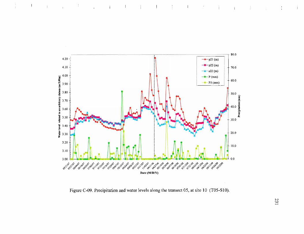
80.0
4.20 -1= ~ --+- p21 (m) I I
410j ~ !, ---- p22 (m)
I + 70.0 -a- s22 (m)
S 4.00 ·'
n __ P(mm)
:5 . P3 (mm)
+ 60.0 ~ 3.90
......
-!!-a ~ 3.80 . - 50.0 ... e t' ~ 3.70 . e ..
0:> of co
~ 40.0 B
= 3.60 s ! 3.50 co 30.0 1! 1 3.40
~ 3.30 ~ 1 I ll' II -...,-,. + 20.0 ~
3.20
:: Jltd~ .~ i J lklkht ~ro ,J: ..,.... ~ . ~ I . ~ -1& \ • 0.0
~ ~ ~ ~ ~ ~ ~ ~ ~ ~ ~ ~ ~ ~ ~ ~ ~ ~ ~ ~ ~ ~ ~ ~ ~ ~ ~ ~ ~ ~ ~ ~ ~~-~~~~~~~#~~~~~~~~~~~~#~~~~~~~~~ ~~~-~-~~~~~~~~~~~~~'-~~~~~~~~~~~~~~~ ~, ~, ~ ~ ~ ~ ~ ~ ~ ~ ~ ~ ~ ~, ~ ~ , ~. ~ ~ ~ ~ ~. ~ ~ ~ ~ ~ ~ ~ ~ ~
Date (M/DIY)
Figure C-09. Precipitation and water levels along the transect OS, at site 10 (T05-SlO).
'a. 'g 110.
N VJ -

4.80
4.70
4.60
4.50
,-. 4.40 a ~ 4.30 OIl
! 4.20 a ~ 4.10 ." t' 4.00
i 3.90 .. Ii 3.80 .e "8 3.70
i 3.60
] 3.50
t 3.40 7i ~ 3.30
3.20
3.10
3.00
--------:---------T---l~~;;ll' 70.0 I I -6-g09 (m) I : :K I
I I I I I I I I I
p23 (m)
-t-p24 (m) 60.0
i ~~~ ><x\ x'Sf ~ 1 xx4 lS< \
'\. .. '" x\ I" l'\ t"tf ·+ Xx . f"\ XX ,v 'c Xx 1 ~ " ~ ~ ++ t +\ ~ .J A Xx I : ++ "\. 1 i\\ ~ tft"~ 1 ~ ... ..!>~ ~t* ++""'+ .. ...! A .\,ttA\~ .:...l(·t .C .. ~A, ·,-.~r~~A,.J~ ~,, "'t .. ~.:.·"""A: " ~:",.. ~~~ I + ++ +
. ~ : + of : 't-+ I ++4. I I I I I I I I I I I I I I I I I I I I I I I
! ~ ! i t ~\~! _.. 1
-6- s24 (m)
50.0
"""*"" p25 (m)
~P3(mm)
40.0 I i ~
30.0 f A.
20.0
10.0
I
f ~'1.w~"J ,.', r . , ... ,~ ~, ) ! ~I ,I ,1m \III?', ~~ , · ,W, III' ,Ei*? '" . ' 0.0
$##$$##~$#$###$~$$#$#$#~#$$$#$~$#$$ ##$$~~$##~####$~~~~$##~~###$~~~###~
Date (MIDIY)
Figure C-IO. Precipitation and water levels along the transect 06, at site 11 and site 12 (T06-S11 and T06-S12).
tv w tv

4.12 -'- glO (m)
4·'1 n --p26(m)
-'- s26(m) ! 3.92 ~ ~p27(m)
s27 (m) '" • e 3.82
.e • "= t> 3.72
~ ~ 3.62 II • 2 'i 3.52 .. t "f 3.42 ..! .. $ -; 3.32
3.22
3.l2 10 Io .......... _h 10 (\ (\J\ (\ (\ (\ (\ (\J\ (\J\ (\ (\ (\ ~ ~ ~ ~ ~ ~ ~ ~ ~ ~ ~ ~ ~~~~~~~~~. ~~~#~~~~~~~~~~~~~~~~~~~ $#~##~###$##~~~###~~##$#$#~~$###
Date (MIDIY)
Figure C-11. Water levels at Site 13 and Site 14, along the transect 07 (T07-S13, and T07-S14).
N W W

5.10
5.00
,..... 4.90
~ ~ 4.80 ~ a = .. 4.70
'1:1
C
t " = " .e 1 ~ ~
4.60
4.50
4.40
.!/ 430 ~ III
~ 4.20
-'-gll (m)
__ p29(m)
-'- s29(m)
4. 10+1~~~~~~~~~~~~--~~--~~--~~--~~--~~--~~--~~--~~
###$#$~$~$-$$$#$##$$$#$#$#$#$## #$$'#~~####$$~$####~$$###$###~~
Date (M/DIY)
Figure C-12. Water levels at Site 15, the transect 08 (T08-SIS).
N I.;J ~

4.92 •
4.82
~~n
~ !4~
e ~ ~52 ~
i4~ ~ -= -4n S . ~
14~ ~
J 4.12 .. 1 ~ 4.02
3.92
3.82 r . ,
--'- g1 2 (m)
___ p31 (m)
--'- 531 (m)
#####$~##$$~$$$~$$#$$#$$##$#$~~~ ~ ,~~~~~~-~~~~_#_~~~~~~~~~ -~~~ -~~~~~;#~ <$'" ~ 1:1 1:1 \;S 'II ' " IJ'" <;;j'"" 1:1 1:1 '3""" 'Or' 1:1 1:1 1:1 ""' \;S 'II ' " , "' " 1:1' <$'" '3""" 1:1 1:1 \;S 1:1 'II ' " "
Date (MlDIY)
Figure C-13. Water levels at Site 16, the transect 09 (T09-S16).
N Vol til

5.50 ---*- g13 (m)
---p32 (m) 5.40
e ---*- s32 (m)
8 5.30 wi
~p33(m)
." s33 (m) .. e 5.20 a .. t 5.10 .. ;5 of 5.00 .. II .. S 4.90 '1:1 .. ... .. t 4.80
'il ... J:! 4.70 .. ~ .. ~ 4.60
4.50
4.40 10 10 10 ..... 10 10 (\ (\ (\ (\ (\ (\ (\ (\ (\ (\ ~" (\ (\ ib -'" ib ib ib ib ib ib ib ~'b ib ib ~~~~~#~~~~~~#~~~~~~~~~#~~~~~~~# $#~##~##~$$#~~~~##~~##~$~##~~~~
Dllte (MIDIY)
Figure C-14. Water levels at Site 17 and Site 18, along the transect 10 (T1O-S17, and TIO-S18).
tv w 0\

4.90
4.80
4.70
4.60
4.50
'i 4.40
~ 4.30
! 4.20
I 4.10 .. .., ~\
:---~--;::===:=:=:::::;----T-~:---------1 80.0 I -k- gI4(m)
-+- p34(m) -k- s34(m) -+- p35 (m) ~s35(m)
p36 (m) -+- 536 (m) --+- P3 (mm)
I I
I I I I
70.0
60.0
50.0
I co t'
i .. :; .e
4.00
3.90
3.80
3.70
! \l ~ ~ i r\ I I
i + i ' . t\ ~ ~ ~ ~ + n. i : \ I \1, I ~ : ~llj' f' 111 ~J ~. " I ~
WO f ' ~ ~ ~, \ ~ : : ,' \ / ' I .' I . • , I ."' • . I I , ~
1) 340 I ! , ~ ;~~ ! ~ ~f~ ~. ~ 3.30 . : .' , : \ I' .. I t...l I I. ;;320 : ·y : .t'I ~ .: : ~ ¥
! ~
3.60
3.50
3.10: : I I
3.00 ' : : I I
2.90: : I I
30.0
20.0
10.0
2.80' , 0.0 b b b b b b ~ b ~ ~ ~ ~ ~ ~ ~ ~ ~ ~ ~ ~ ~ ~ ~ ~ ~ ~ ~ ~ ~ ~ ~ ~ ~ #~~~#~~~~~~~~~~~~~#~~~~~~~~~~~##~ ~#~#~#######$#~~~$~##~#$#$~~#$~~~
Date (MIDIY)
Figure C-1S. Precipitation and water levels at Site 19 and Site 20, along the transect 11 (Tl1-SI9, and Tl1-S20).
N W -..J

5.30
5.20
5.10
5.00
4.90
l 4.80 vi ! 4.70 e S 4.60 • .... t' 4.50
~ 4.40 • iii 4.30 S ! 4.20
~ 4.10
1 4.00
~ 3.90 • ~ 3.80
3.70
3.60
I I I I I I I I
! 1 \
, ,.~
I ---- 'I5(m) ~ p39 (m)
--+- s39 (m) --p38(m)
s38 (m) --'- p37 (m) --+- s37 (m) -+-- P3 (mm)
~~.
90.0
80.0
70.0
60.0 e e --50.0 .~
-i 40.6 ~
30.0
20.0
10.0
3.50 ~ .. _ .. ~..., oo ~ ,~ ,"I ~t"i"\III~ ,i ~ .....,.... hi iY ~... .
~ ~ b b b b ~ ~ ~ ~ ~ ~ ~ ~ ~ ~ ~ ~ ~ ~ ~ ~ ~ ~ ~ ~ ~ ~ ~ ~W~~$~$~~~~~~~~~~~~#~~~~~~~~~ ~#~#~~~##$~~#$##~$$~$$~~~####
Date (M/DIY)
Figure C-16. Precipitation and water levels at site 21, Site 22, and site 23 along the transect 12 (TI2-S21, T12-S22, and T12-S23).
tv w 00


e ~ ! E ! 01 ~
t'
i 01 1:1 01
!
I ] .. $ .. ~
5.20
--.- g16 (m) 70.0
'IOJ ~l\ p40 (m)
--'- s40 (m)
5.00 ~P3(mm) 60.0
4.90 50.0
4.80 40.0
4.70
30.0
4.60
20.0
4.50
10.0 4.40
4.30 1''' ~ ,a. •• • ,.......... ......... , • ..... ........ • .•••• ~. , •• ., .. ,.... H ,. ' 0.0
b b b .b b b b b ~ b b ~ ~ ~ ~ ~ ~ ~ ~ ~ ~ ~ ~ ~ ~ ~ ~ ~ ~ ~ ~ ~ ~ ~~~~~~~~ff~~~~~~~~~#~~~~~~_~~'~~~~~~ ~~-~~~~~~~~~~~~~~-~-~~-~~~~~~~~~~~~~~ ~, ~ ~ ~ ~ ~ ~ ~' ~ ~ , ~ ~ ~ ~ ~ ~ ~ ~ ~ ~ ~ ~ ~ ~. ~ ~ ~ ~ ~ ~ ~ ,
Date (MlDIY)
Figure C-17. Precipitation and water levels at site 24, along the transect 13 (T13-S24).
! 1:1
~
i ~
jI.,
N w \0
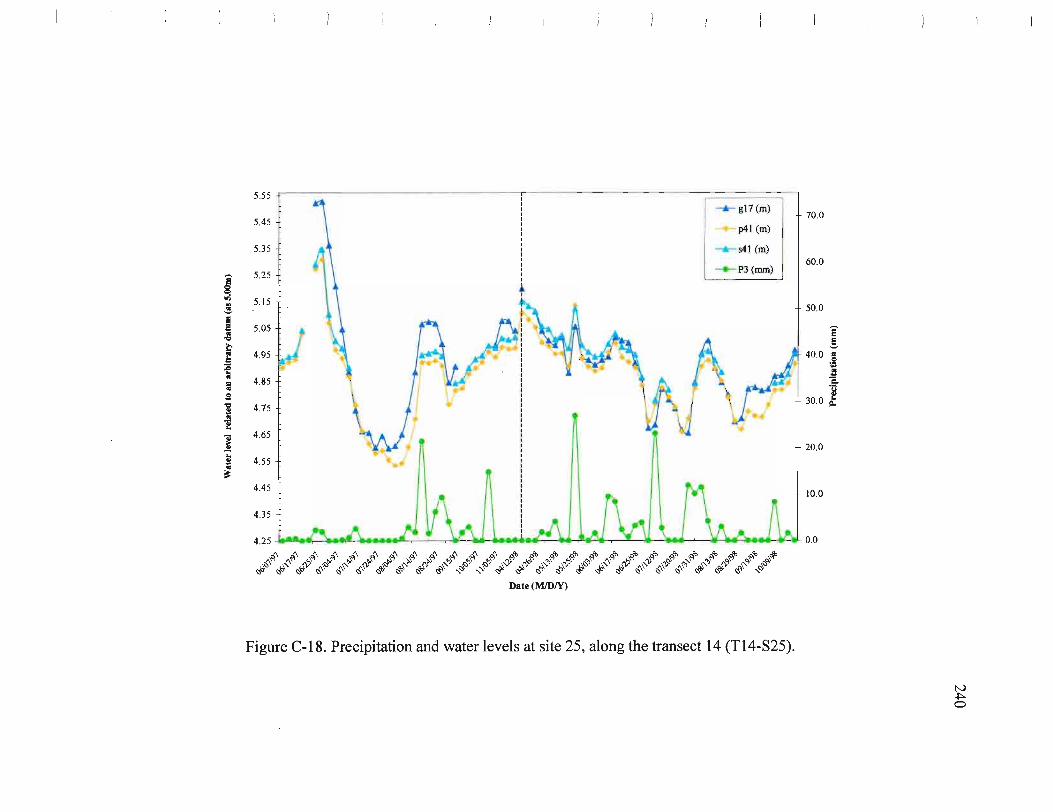
i ~ '" ! I!! ! .a to j .. .. ; S
! .. '1i .. ] .. a .. it;
5.55 , -'- g17 (m)
I + 70.0 , - p41 (m) 5.45 +
5.35 + ., -'- s41 (m) I + 60.0
5.25 --+-P3 (mm)
5.15
5.05 i !
40.0 § :;: f\ t \A 30.0 !
4.95
~ 4.85
4.75
4.65 . .... ~ 71' I I 1\ + 20.0
::: LA.~ ..... ,) VWl .. LJ LJ:J lJ~.A1 ::' 425 r-. r-. r-. r-. r-. r-. r-. r-. r-. r-. r-. r-. ~ ~ ~ ~ ~ ~q, ~ ~ ~ ~ ~ .... ~ ~ ~ ~ # # ~ ~ # ~ ~ ~ # # ~ ~ ~ ~ ~ ~ ~ ~ ~ ~ ~ ~- ~ ~ $$~~~#~$#~#~##$#$$#~#~$##~
Date (M/DIY)
Figure C-18. Precipitation and water levels at site 25, along the transect 14 (T14-S25).
N ~ o

,
p42 (m) I + 80.0 I
1 I ::: 1
i I
---.- s42 (m)
I
I I
I I
I I
I
~p43 (m) I + 70.0
I
: I I
.¥ p44 (m)
4.65 I
!.I I 455 + I ~p45(m)
I + 60.0 ~ --P3(mm) ~ 4.
45 1 It! 435 ! .
50.0 i !. t:I
~ 425 -R
0 -;: !!
•
40.0 ~
."
t' 4.1 5
~ of 4.05 •
t
"" t:I
S 3.95
1 i 3.85 30.0
+ 20.0 /I
1)
fW' T ~ 3.75 .. F ~ 3.65
355 ~i&d~ i 3 .45 ~ .. k 3.35 l\.....eA JVWLLJWUU:OoO
b _" 10 10 !o .Jo !o r-. r-. (\ (\ (\ r-. (\ r-. (\ (\ (\ (\ !b !b !b !b !b 10 10 10 10 10 ~~~~~~~~~~~~~~~~~~~~~~~~~~~~ff '$~##'~'$"#~##'#$$'#"'~~$'~
Date (MJDIY)
Figure C-19. Precipitation and water levels at site 26 along the transect 15 (TI5-S26).
N +:--
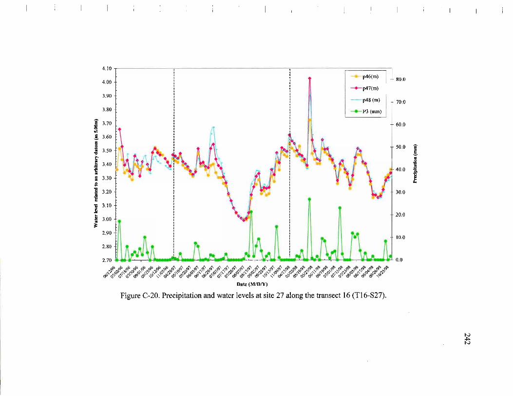
4.10 --- p46(m)
I + 80.0 4.00 -+-p47(m)
3.90 - p48 (m) I t 70.0
3.80 -e- P3 (mm)
I 3.70 + 60.0 vi ! 3.60
i l~ I r~J~ 50.0
.; 3.50 ~~ I
f 3.~ ~ . ;f~~ 40.0 I I
= 3.30 j '. I I I
S : I I
! 3.20 l I I 30.0 I
t 11 3.10
" .lo. m /I II + 20.0 .. ! 3.00 ~
::: ~~ 2.70 1
1 , ~'" A VlJL J ,.J LI1d U~ ~ :000 b b b b b b~ b ~ ~ ~ ~ ~ ~ ~ ~ ~ ~ ~ ~ ~ ~ ~ ~ ~ ~ ~ ~ ~ ~ ~ ~ ~ ~ ~ ~ ~ ~~~~~~~'.,~#~ ~~~#~~M~~~~~~~~#~~~~~~~~-~~~ ~~~~~~y~~~~~~_~_~~~~~'~~~V~~~~~_~~~~~~~~~§~~ ~. ~ ~ ~ ~' ~ ' ~ , ~. ~ ~,~ ~ ~ ~ ~ ~ ~ ~ ~ ' ~ ' ~ , ~. ~~,~, ~, ~ ~ ~ ~ ~ ~~' ~' ~
Dllte (MIDI¥)
Figure C~20. Precipitation and water levels at site 27 along the transect 16 (T16-S27).
I .I ... i ~
~
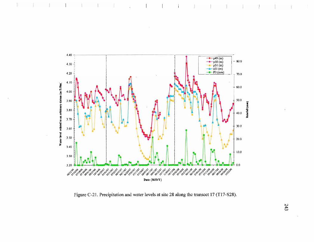
4.40 -+- p49(m) -+-p50 (m) I + 80.0
4.30 + 111 _ pSI (m)
--'- s51 (m)
4.20 1. ~ ~ It t -+-P3 (mm) I r 70.0
" 4.10
~ rr i • i ~ + rr~\1 .,. L' ~ m '\\., .. In + 60.0 iii ! 4.00
J::D~ ~ n·1 , ·1'\ ,A r! 1 ~ ~ ~ ~l~ \ Aso.o ! 'E : ~ t I ~ A I : i V 40,0 J!
Ii \J\ n~ \ " ! ~ S 3.70
! t 1£ I - I I 11 i "\ j; I t' I I I \I .. ~ I ~ + 30.0 ~ 3.60 .. ~ 3.50 t . v nr ~.. II 'II 1/. ~ 1 + 20.0 i
• 3~ ~~ , \ ~f VWl ' ~liJlJ1.j 1 1 10.0
:::: ~ .. 1111~1II~ 1 ill 0.0
######~$$$$#$$#$##$##$####$$#$$#$$~$$ $$~~#####~##$#$~#####~~####$$$~##$~#~
Date (MID/y)
Figure C-21. Precipitation and water levels at site 28 along the transect 17 (T17 -S28).
~ w
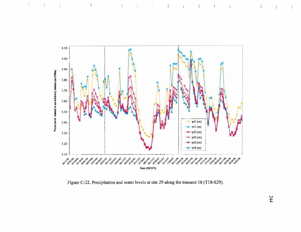
I ! ~ .; t' e ~ .. Q .. g
! ~ 1 .. ~
~
4.10
4.00
3.90
3.80
3.70
3.60
3.50
340 1 111:
1 [W pSI (m)
-'- s51 (m)
3.30 -*-p52(m)
~p53(m)
3.20 l ~ -*-p54(m)
-'- s54(m)
3.10 Io-h Io..h_h..h"lo (I-L\ (I (I (I-L\£\ (I (I.f\£\.f\ (I (I (I.f\!b !b,,'b!b!b!b!b!b!b!b!b!b!b!b 1i tV" ~"" ~"~".,~ ~~. ~'" ~~ . ~'" .,f' ~'" '\~. PI~ (If' 'If' ~.., . (I't' '\~~'" rV'" ~'" ~~ . "'~ # PI" f\~ ,,OJ oj{'l ~Oj .,~ i'i-Oj I:}Oj '\~ J<Oj ~Oj oj-Oj
$$~######~##$#$$###~#~v~~$#$$$$###~#~ Date (MIDIY)
Figure C-22. Precipitation and water levels at site 29 along the transect 18 (T18-S29).
tv t

5.20 I I 60.0
5.10
5.00
4.90
I~~ ! S ~4~ ~
--.-...- gl9 (m)
--.-...- s56 (m)
--P3(mm)
p56 (m) __ p57(m)
50.0
40.0
e .! .. .. ~
~4~ ~
30.0 ~
=4~ S ] ~4~ 'il
li 4.30
~ ~ 4.20
4.10
20.0
10,0
4.00 ~ . ~ "e , . ............. ...... • , •• ........- ... -.e< "a... , ~L"' •• I 0.0 ~ ~ ~ ~ ~ ~ ~ ~ ~ ~ ~ ~ ~ ~ ~ ~ ~ ~ ~ ~ ~ ~ ~ ~ ~ ~ ~ ~ ~ ~ ~ ~ ~ ~ ~~~~~~~~~~~~~~~~~#~~~~~~~~~~#~~#~~~ ~~~~~ ,~~~.~~~~~~~~~~.~~~~~~~~~~~~~~~~~~~ ~ ~ ~ ~ ~ ~ ~ ~ ~ ~ ~ ~ ~ ~ ~ ~ ~ ~ ~ ~ ~ ~ ~ ~, ~ ' w ~' ~ ' ~ ~ ~ , , ,
Date (M/DIY)
Figure C-23. Precipitation and water levels at site 30 along the transect 19 (T19-S30).
... '~ CI.o
N .J:o. VI
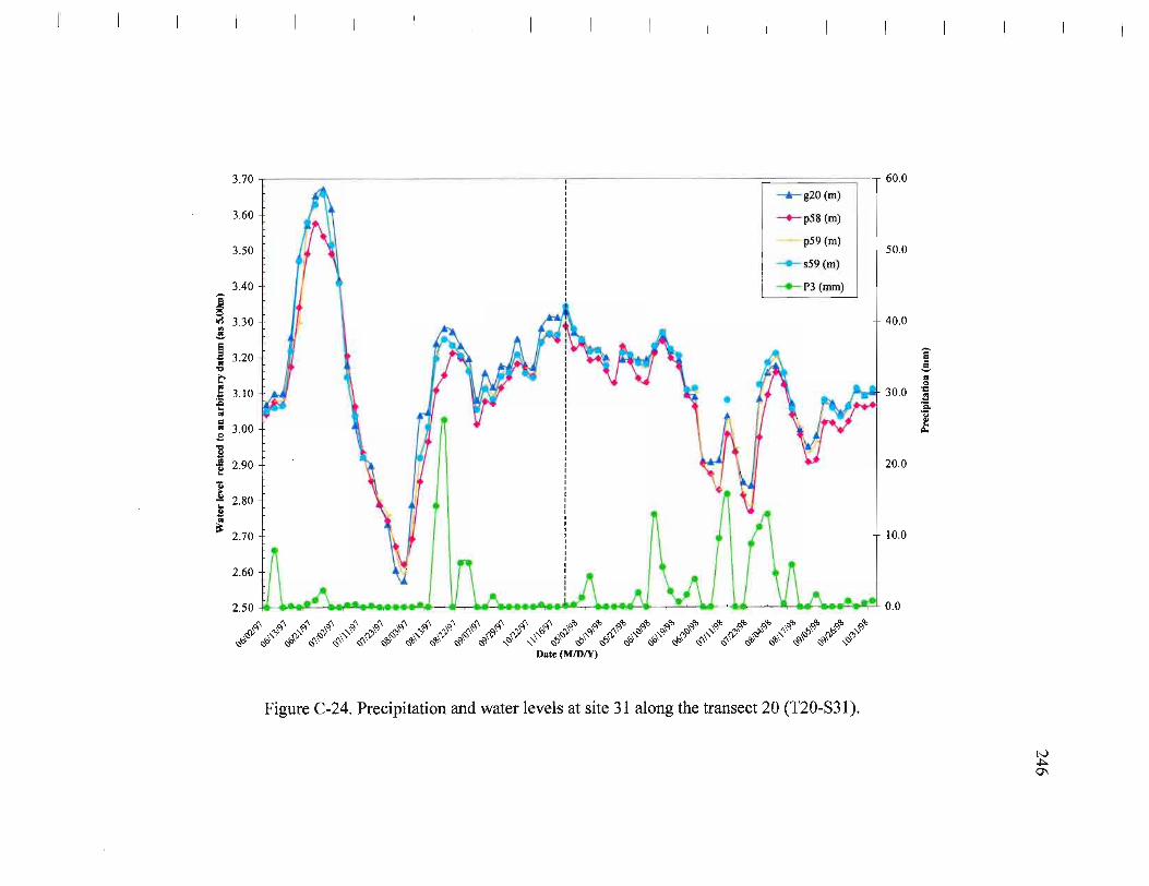
3.70 60.0 ----, ---.- g20 (m)
3.60 --+- p58 (m)
3.50 -- p59 (m)
I t 50.0 -+-- s59(m)
3.40 -+-- P3 (rom)
l ~ 3.30 + ' /~
-----'
40.0 .!!, 5 ~ 3.20 ..:0
t' ~ 3.10 30.0 :E .. .. i 300 ~ . 'j ~ 2.90 20.0
OJ ~ ';: 2.80 a .. ~ 2.70 10.0
2.60
2.50 ~ ....... .. ~ ••• ,....... JJ I..( .. , ..... , ....... , ...... 'e .. .. .. , .. ...... .,......-' 0.0 ~ ~ ~ ~ ~ ~ ~ ~ ~ ~ ~ ~ ~ ~ ~ ~ ~ ~ ~ ~ ~ ~ ~ ~ ~ ~ ~ ~ ~ ~ ~ ~ ~ ~ ~ ~ # ~ ~ ~ # ~ ~ # ~ ~ ~ # ~ ~ ~ ~ #$#~~~#~###~~####$#~~~~##~
Date (M/DIY)
Figure C-24. Precipitation and water levels at site 31 along the transect 20 (T20-S31).
i ! c ..
i II.
~ 0\

3.85 -
3.75
3.65
'i 3.55 8 ! 3.45
j 3.35 .; t' 3.25
i 3.15 " a ; 3.05
t 2.95
]2.85 .. i 2.75 ~
2.65
2.55
-+- gZl (m)
p60 (m)
-+-s60(m)
.......... p63 (m)
~P3~
'\
60
-l- 50
40
I a
30 ! .; CI.
.~
=-
20
10
2.45 ~J ~ A 1 U It. ... , .... U L, .. /J v \j ,U 'J ~A.~~ 0 2.35 • • ... , ••••• ,... , ~ ~ ~ ~ ~ ~ ~ ~ ~ ~ ~ ~ ~ ~ ~ ~ ~ ~ ~ ~ ~ ~ ~ ~ ~ ~ ~ ~ ~ ~ ~ ~ ~ ~ ~ ~ ~ ~ ~ ~ ~ ~ ~ ~ ~ ~ ~ ~ ~ -~ ~ ~ ~ ~ ~-~-~~~~~~~~~~~-~~~~-~~~~~§~~~~ ~, ~ ~ ~. ~ ~ ~ ~ ~ ~ ~ ' ~ , ~- ~ ~, ~ ~ ~ ~ ~ ~ w ~ ~ ~ . ~
Date (MiDty)
Figure C-2S. Precipitation and water levels at site 32 along the transect 21 (T21-S32).
IV ~ -....l
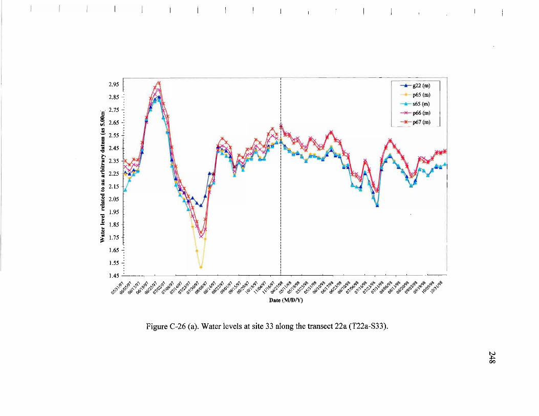
2.95 + .J"'! -+- g22(m)
2~ 1 f\ , p65 (m) , ,
-+- s65 (m) , , ~. 2.75
, ~p66(m)
, , , , -"'- p67(m) iii 2.65 - '" :J e 255
-.e .a 2.45
t' f 2.35
.1:: J:l ~ 2.25 1:1
~ 2.15 -i 2.05 41
.:: 1.95 ~ ~ 1.85 .! -; 1.75
\) 1.65 J 1.55 i 1.45
$$#$$#$$$$$$#$$$$~$$$$$$$~##~##$##$#$~$ ~~-~-~-~~~~~~~~~~~~~$~~~~~~-~~~~#~~~~~~~~#~ ~, ~ ~ ~ ~ ~ ~ ~ ~ ~ ~ ~ ~ ~ ~' ~ ' ~ , , ~- ~J ~ ~ ~ ~ ~ ~ ~ ~ ~ ~ ~ ~ ~ ~ ~ ~ ~ ~
Date(M/DN)
Figure C-26 (a). Water levels at site 33 along the transect 22a (T22a-S33).
~ 00
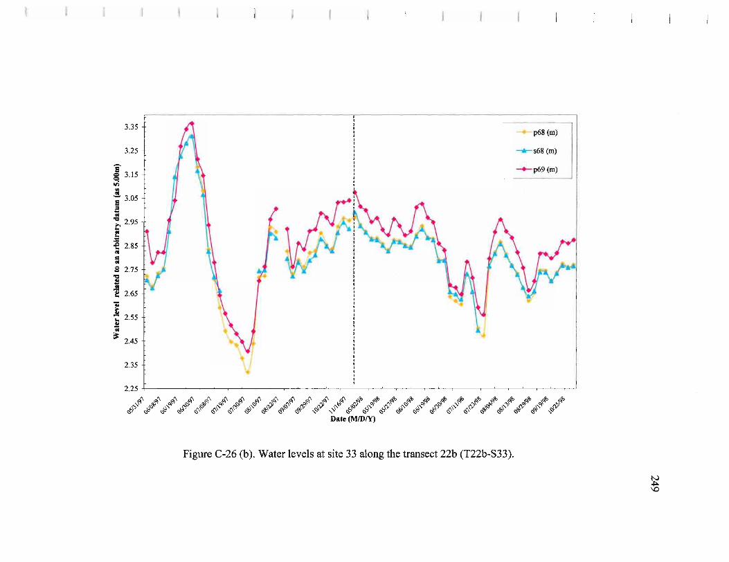
3.35 t f\ - - p68 (m)
3.25 --'- s68 (m)
'i -+-p69 (m) g 3.15 OIl ; e 3.05
~ • t. 2.95
~ of 2.85 • Cl • S 2.75 ~ .a ~ 2.65 .. t ';: 2.55 .. -• ~ 2.45
2.35
2.25 ~ ~ ~ ~ ~ ~ ~ ~ ~ ~ ~ ~ ~ ~ ~ ~ ~ ~ ~ ~ ~ ~ ~ ~ ~ ~ ~ ~ ~ ~ ~ ~ ~ ~ ~ ~ ~ # ~ . ~ # ~ ~ ~ ~ ~ ~ ~ ~ # # ~ ~#$#~##$$##~~#$$$$#~~~$###
Date (MIDIY)
Figure C-26 (b). Water levels at site 33 along the transect 22b (T22b-S33).
N ..J;>.. \0

I ! ~ • ... to J; :e • ., .. S
i i 1)
] .. .!I .. ~
5.25 -r ~ """'- g24 (m)
515
1 M\ p73 (m)
"""'- s73 (m)
5.05
A ~p74(m)
4.95 -'lie- p77 (m)
4.85
4.75
4.65
4.55
4.45
4.35
4.25
4.15
4.05
3.95
3.85
~ ~ ~ ~ ~/ ~ ~ ~ ~ ~ ~ ~ ~ ~ ~ ~ ~ ~ .~ ~ ~ ~ ~ ~ ~ ~ ~ ~ ~ ~~~#~ ~~~~~~~~~~~~~~. ~~~&~~~~#~ ~ ~ ~ ~ ~ , v ~ ~ ~ ~ ~ ~ ~ ~ ~ ~ ~ ~ ~ ~ ~ ~. ~ ~ ~ ~ ~ ~ V Date (MIDI¥)
Figure C-28. Water levels at site 35 along the transect 24 (T24-S35).
tv VI ..-

500.00 ---, I 0.30 -r---------------------,-----;::=================~I
-+- dp75 (rn) ---.- ds75 (rn)
0.25 dp76 (rn) ---'- ds76 (rn) + 450.00
0.20
1 0.15
~i ; wi 0.10 ... :I Ii-.. II [~ 0.05
; j i:s 0.00 " 11 II " i; -0.05 II] II .. ~ 'E -0.10 is
-0.15
-0.20
-0.25
---.- Q (rnA 3/s)
........ .................. .. ~-.
-0.30 +-f ~-r-'--,-~..,....-'--r~~"---,~--.-~~-.-~~---r~-r-'--,-~..,....-'--r~-,--"---,~--.-=-~--,-:=---.,......---r--4-
!o !o !o !o !o !\ !\ !\ !\ !\ !\ !\ f>I'\ !\ !\ !\ !\ !\ fb fb fb fb fb fb fb fb fb fb fb ~~~~~~~~~~#~~~~~~~~#~~~~#~~~~ #~$#~##$##$~~ff$##~#$$$~#~#~~~
Date (M/DIY)
400.00
350.00
300.00
250.00
200.00
150.00
100.00
50.00
0.00
,., ., < .! .. !." .. ~ :;; II
! '"
Figure C-29 (a). Differences between stream gauge and water levels at site 36 and site 37 along the transect 25 (T25-S36 & S37).
tv VI tv

0.25 + I -+-dp75 (m)
-'-ds75 (m) 50.0
0.20 + I \ I ><; I I dp76 (m)
0.15 1 I ~ I ~ It n' l -'-ds76(m)
[ _ \ ,.. \ II --P3 (mm)
I ~ 0.10
• II 1 j 0.05
t~ i i 0.00
;~ i: -0.05
is til !. -0.10 .. 1
!5
40.0
30.0
20.0
Q -0.15 10.0
-0.20
-0.25 r..-."" ...... i ............... !J. w ........... il ..... "' - .. , .. , • il .... ..,.. 0.0
#~$$$~$$~$$~$$##$#$$$##,~##$$~~# ###~#~~##$#~#####$$#~~#,#~$#~~#
Date (MJDIY)
E .! = -! ~ .S-
!
Figure C-29 (b). Precipitation and differences between stream gauge and water levels at site 36 and site 37 along the transect 25 (T25-836 & 837).
tv Vl W
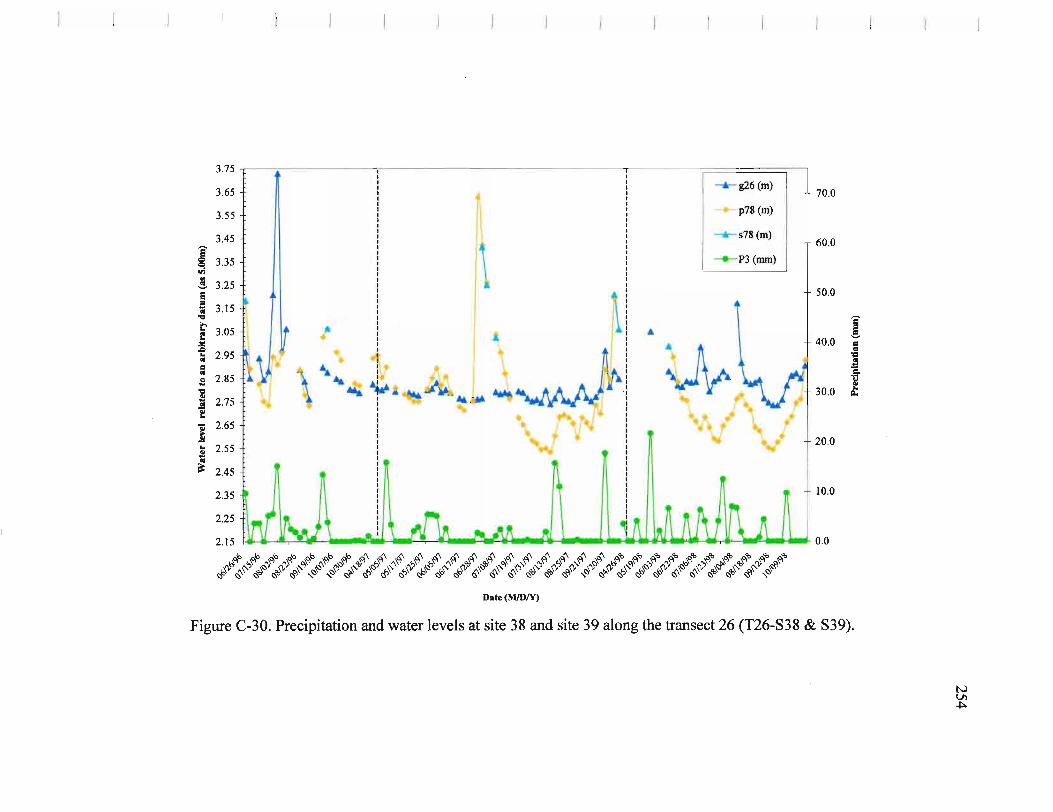
70.0
60.0
50.0
40.0
30.0
20.0
10.0
f ~ ~ M ,~ ..... ,'.t.J~ ,tj' -"'rtW.....,....... I _ .... Jf~w .. l.j , iII -...,W_ 0.0
b b b b ~ b b ~ ~ ~ ~ ~ ~ ~ ~ ~ ~ ~ ~ ~ ~ ~ ~ ~ ~ ~ ~ ~ ~ ~ ~ ~~~~~~~~~.~~~~~~#~~~~~~#~~~~-~~~~ -~~~~~~~~~~~-~-~~~~~~~~~-~~-~-~~~~~~~' ~ ~ ~ ~ ~' ~ ~ ~ ~, ~, ~ ~ ~ ~ ~ ~ ~ ~ ~ ~ ~ ~ . ~, ~ ~ ~ ~ ~ ~ ~ ' ~
Date (MIDIY)
I J ! .eo ~
CI.
Figure C-30. Precipitation and water levels at site 38 and site 39 along the transect 26 (T26-S38 & S39).
N VI ~

5.50 I 4.50 , 5.40 : -+- g26 (m) --lIf- p79 ~) 5.30: I
-+- s79(m) p80 (m)
j~ ,J--~ ~~~-J\.-Ho(m~ )4,:;":::::: ~ 4:80 ! f\ ~'\. i 111 I I
'" 4.70 ~ : I
i 4.60 \ :
i : :~~ If ~ 1/>"'-i::;~ ~.( 1 I \ : 4.10 1\ j-.. \ s 4.00 ~ Al-i ~ ::~ • ..,.. f .. ['M: '-........ ! 3.70 ~ I ... A 1 3.60 ~ ~~ I - ~ i 3.50 .f ~ ~ -Lt'K. \ ~ ~ 3.40 'K. I 'K. :t.:t:.;:
3.30 ~ I , ~ 3.20 'K. :
~
3.10 : I
3~ \ :
• ~
~
~
~.
4.00 ;;;
I 3.50 !
J 3.00 t'
i .. • 2.50 Ii ~
.2.., iii
2.00 ! ~ ~
-= 1.50 ~
'; ~
1.00 ~
i 0.50 rLl
2.90 \ ~_ : 2.80 ... ~~ ,..Jw.~~ ....... -."".n..£1l..o ... 2.70 0.00
b ~ ~ ~ b ~ ~ ~ ~ ~ ~ ~ ~ ~ ~ ~ ~ ~ ~ ~ ~ ~ ~ ~ ~ ~ ~ ~ ~ ~ ~ ~ ~ ~~~~~~.,~~~~#~~~~~~~~~~~~~~#~~~~~~ ##~$#~~~##$~###~~~##~~#$$$~~###~~
Date(MJDN)
Figure C-31. Water levels at site 40 along the transect 27 (T27-S40), and comparing with stream gauge changes at transect 28 and 29.
~ VI

4.95
4.85
4.75
4.65
j 4.55 ! ! 4.45 ~
i 4.35 of • = 4.25 .e ~ 4.15
j 4.05
.Ii ~ 3.95
3.85
3.75
I I I I I I I I I
-'-g27 (m)
-+-p82(m)
-'- s82(m)
-+-p83 (m)
883 (m)
3.65+~~~~~~~~~~~~~~~~~~~-r~~~~~~~~~~-r~~~~~~~
b b b ~ b b _h ~ b ~ ~ ~ ~ ~ ~ ~ ~ ~ ~ ~ ~ ~ ~ ~ ~ ~ ~ ~ ~ ~ ~ ~ ~ ~ ~ ~ ~ ~ ~ ~ ~~~~#~~~~~~~.~~~~~~~~~~~~~~~~~~#~~~~#~#~~ #$~#~#~#~#~#$##$#~$~~#####~#$$~#~~#~###~
Date (MIDIY)
Figure C-32. Water levels at site 41 and site 42 along the transect 28 (T28-S41 & S42).
IV Vl 0\

4.45 ~ - I I I I
4.35
4.25
l4.15 iii .. .,!!. Ei 4.05 ~ .., t' 3.95 .~ ,Q
:; 3.85 ;l .s 1 3.75
~ OJ 3.65 } ... .. ~ 3.55
3.45
3.35
I I I
t i BI . ~
1\
I I I I I I I 1 I I I I I I I I I
'1!' I I I I
hi ~ ~
~ ~ I
~ i I I I I I I I I
~g29(m)
~p84(m)
p85 (m)
3.50
3.00
2.50 g ~ .. .. ~
2.00 iI,
j 1.50
1.00
3.25 r I I 0.50 !o -",.)0 !o !o !o !o (\ (\ (\ J\ (\ (\ (\ (\ (\ (\ (\ (\ (\ (\ ib ib ib ib ib ib ib ib ib ~~~~~~~~~~~. ~~~~~~~~~~~~~~~~~~-~ -~~~~~~~-~~~~~-~~~~~~~~~~~~~~~~~~ ~ G ~ ~ ~ ~ ~ ~. ~, ~ ~ G ~ ~ ~ ~ G ~ ~ ~ , ~, ~, G ~ ~ ~ G ~ , ~
Date (MIDIY)
Figure C-33 (a). Water levels at site 43 along the transect 29 (T29-S43), and comparing with main channel water level changes at transect 28.
tv VI -....l

I .. ,!!. e a • " t'
i .. '" .. S 1 ~ ] .. $ II
~
4.10 60.0 I I
-'-g29(m)
4.00 -+- p84 (m)
3.90 -+- p85(m) I ~ 50.0
-+- P3 (mm)
3.80 ~I 40.0
3.70
3.60 30.0
3.50
3.40 20.0
3.30
3.20 10.0
3.10
3.00 r ~ , ~~ , j , .~ rw _~"l {'_W~~.... ! WW"M~W __ W i ~ __ 0.0
~~~.~~~~~~~~~~~~~~~~~~~~~~$~~~~ ~~~~~~~~~~~ ,~~~~~#~~~~~~~ ,~ ~ ~~~# ~ ~ ~ ~ ~ ~ ~ ~ ~ ~ ~ ~ ~. ~ ~ ~ ~ ~ ~ ~ ~ ~ ~ ~ ~ ~ ~ ~ ~ ~
Date (M/DfY)
Figure C-33 (b). Precipitation and water levels at site 43 along the transect 29 (T29-S43).
B -! '" 0 ~
.~ "" .~ ~
IV VI 00

4.35 4.50
4.25
4.00 4.15
l4.05
~ wi
! e 3.95
i to 3.85 ~
I ; 3.75 {
3.50
g 3.00 ~
!&
~ ~
S
r65
j ~w~ p86 (m) -.; 3.55 I , ~ , , -+-p87 (m) ~ ., , .. 3.45 ,
~ , """'- s87(m)
, , ,
2.50 ! rn
2.00
, , --*- p88 (m) , , 1.50
, , """'- g30(m) 3.25 , , , , ,
335
1 3.15 ~-r~~~~~~~~~~~~~~~~~~-r~~~~~,-~~~~~~~~I 1.00
#########$$$$$$$~$#$#$$####$#~ ~~~~~~~~~~~~~.~~~~~~~~~~~~~~~~~~# ~ ~ ~ ~ ~ ~ ~ ~ . ~, ~ ~ ~ ~ ~ ~ ~ ~ ~ ~ ~ , ~ ~ ~ ~ ~ ~ ~ ~ ~
Date (MIDIY)
Figure C-34 (a). Water levels at site 44 along the transect 30 (T30-S44), and comparing with stream water level changes at transect 30.
tv VI IC)

4.40
4.30
84.20 i Ifi '" 4.10 ~ E! S 4.00 01
"e
C3.90 f .... :e 3.80 01
= : 3.70 .... "e .. ~ 3.60 'E 1! 3.50 J!
~ 3.40 01
~ 3.30
3.20
•
--+- p89 (m)
589 (m)
--+-p90 (m)
-'-590 (m)
-'-g30 (m)
3.10+r~~~~~~~~~~~~~~~~~~~~~~~~~~~~~~~~~~~~~~~
#########$$$$$$$~$#$t$$$#$$##~ ~~~~~~~-~~~~-~~~~~#~#~~~~~~~~~## ~ ~ ~ ~ ~ ~ ~ ~ . ~ J ~ ~J ~ ~ ~ ~ ~ ~ ~ G ~ , ~ ~ ~ ~ ~ ~ ~ G ~
Date (MIDIY)
Figure C-34 (b). Water levels at site 45, 46, and 47 along the transect 30 (T30-S45, S46, and S47), and comparing with stream water level changes at transect 30.
N 0'1 o

261
Appendix D: Results of Statistical Analyses
Table D-1. Correlation analyses between monitoring sites and stream gauges .. ... 262
Table D-2. Parameters of simple linear regression analysis ............ . ...... . ....... 264
Table D-3. Parameters of multiple linear regression analysis .................. . ...... 266
Habitat Class Type and ID
Habitat ID
Habitat ID
Type Subtype
Main Sandbar; channel 0 braided 0 (MC) stream
Side-channel 11
Side-channel 1
(SC) (SC) Tributary 12
(TB) Connected Backwater 21
Backwater 2 (CB)
(BW) Disconnected Backwater 22
(DB) Permanent
Slough 31 Slough 3
(PS) (SL) Intermittent
Slough 32 (IS)
Riparian Pond 41 Pond
(RP)
(PN) 4 Wet Meadow
Pond 42 (WP)

262 Table D-l. Correlation analyses between monitoring sites and stream gauges
Habitat Transect Obsv. by Kendall's (t) Prob>lt l Class Site ID Well ID Variable
31 TOI -SOI pOl (m) gOl (m) 0.4471 <.0001 31 TOI -S01 sOl (m) gOl (m) 0.1871 0.0194 22 TO I-S03 p06 (m) g02 (m) 0.8089 0.0000 22 T01-S03 s06 (m) g02 (m) 0.7156 <.0001 21 T02-S04 p09 (m) g03 (m) 0.8788 0.0000 21 T02-S04 s09 (m) g03 (m) 0.7981 <.0001 21 T02-S05 plO (m) g04 (m) 0.8918 0.0000 21 T02-S05 slO (m) g04 (m) 0.8348 <.0001 32 T31-S06 p11 (m) g04 (m) 0.5856 <.0001 32 T31-S06 sl1 (m) g04 (m) 0.0741 0.8016 32 T3 1-S06 p12 (m) g04 (m) 0.3588 0.0046 32 T31 -S06 s12 (m) g04 (m) 0.4021 0.0445 42 T32-S49 p13 (m) g04 (m) 0.7893 <.0001 42 T32-S49 s13 (m) g04 (m) 0.2029 0.4582 21 T32-S50 p14 (m) g04 (m) 0.7204 <.0001 21 T32-S50 s14 (m) g04 (m) 0.8377 <.0001 31 T03-S07 p16 (m) g06 (m) 0.3054 <.0001 31 T03-S07 s16 (m) g06 (m) 0.0873 0.1940 22 T04-S08 p19 (m) g08 (m) 0.8926 0.0000 22 T04-S08 s19 (m) g08 (m) 0.7908 0.0000 32 T04-S09 p20 (m) g08 (m) 0.5659 0.0000 32 T04-S09 s20 (m) g08 (m) 0.3807 0.0004 31 T05-SlO p22 (m) g08 (m) 0.4303 <.0001 31 T05-SlO s22 (m) g08 (m) 0.3450 <.0001 41 T06-S12 p24 (m) g08 (m) 0.3263 <.0001 41 T06-S12 s24 (m) g08 (m) 0.4058 0.0370 21 T07-S13 p26 (m) glO (m) 0.8187 0.0000 21 T07-S13 s26 (m) gl O (m) 0.7575 0.0000 21 T07-S14 p27 (m) gl O (m) 0.7127 0.0000 21 T07-S14 s27 (m) glO (m) 0.6671 0.0000 22 T08-S15 p29 (m) gl1 (m) 0.8257 0.0000 22 T08-S15 s29 (m) gl1 (m) 0.6274 <.0001 21 T09-S16 p31 (m) g12 (m) 0.8361 0.0000 21 T09-S16 s31 (m) gl2 (m) 0.6982 0.0000 21 TlO-S17 p32 (m) gl3 (m) 0.7774 0.0000 21 TlO-S17 s32 (m) gl3 (m) 0.6469 <.0001 21 T I0-S18 p33(m) gl3 (m) 0.8919 0.0000 21 TlO-S18 s33 (m) gl3 (m) 0.8422 0.0000 12 Tll-SI9 p34 (m) gl4 (m) 0.7703 0.0000 12 Tll -SI9 s34 (m) gl4 (m) 0.7522 0.0000 42 Tll-S20 p36 (m) gl4 (m) 0.5811 0.0000 42 Tl1-S20 s36 (m) gl4 (m) 0.5742 0.0002 11 Tl2-S21 p39 (m) glS (m) 0.7806 <.0001 11 Tl2-S21 s39 (m) glS (m) 0.6626 <.0001 41 Tl2-S22 p38 (m) gl S (m) 0.3075 0.0080 41 Tl2-S22 s38 (m) glS (m) 0.2471 0.0342

263 Table D-l. Correlation analyses between monitoring sites and stream gauges ( continuous)
41 Tl2-S23 p37 (m) g15 (m) 0.5796 <.0001 41 Tl2-S23 s37 (m) g15 (m) 0.2094 0.3162
11 Tl3-S24 p40 (m) g16 (m) 0.6682 <.0001
11 Tl3-S24 s40 (m) g16 (m) 0.8044 <.0001 22 Tl4-S25 p41 (m) g17 (m) 0.8213 0.0000 22 Tl4-S25 s41 (m) g17 (m) 0.6819 <.0001 22 Tl5-S26 p42 (m) g17 (m) 0.7484 0.0000 22 Tl5-S26 s42 (m) g17 (m) 0.7004 <.0001 32 Tl7-S28 pSI (m) g17 (m) 0.6761 <.0001 32 T17-S28 s51 (m) g17 (m) 0.5482 <.0001 31 Tl8-S29 p54 (m) g17 (m) 0.5617 <.0001 31 Tl8-S29 s54 (m) g17 (m) 0.2518 <.0001 21 Tl9-S30 p56 (m) g19 (m) 0.8365 <.0001 21 Tl9-S30 s56 (m) g19 (m) 0.6495 0.0009 21 T20-S31 p59 (m) g20 (m) 0.9344 0.0000 21 T20-S31 s59 (m) g20 (m) 0.8640 0.0000 11 T21 -S32 p60 (m) g21 (m) 0.8831 0.0000 11 T21 -S32 s60 (m) g21 (m) 0.8459 0.0000 11 T21-S32 p61 (m) g21 (m) 0.6943 0.0000
11 T21-S32 s61 (m) g21 (m) 0.8617 0.0000 11 T21-S32 p62 (m) g21 (m) 0.7313 0.0000 11 T21-S32 s62 (m) g21 (m) 0.7548 0.0000 11 T22-S33 p65 (m) g22 (m) 0.9400 0.0000 11 T22-S33 s65 (m) g22 (m) 0.9212 0.0000 11 T22-S33 p68 (m) g22 (m) 0.9511 0.0000 11 T22-S33 s68 (m) g22 (m) 0.8995 0.0000 21 T23-S34 p71 (m) g23 (m) 0.9070 0.0000 21 T23-S34 s71 (m) g23 (m) 0.6888 <.0001 21 T24-S35 p73 (m) g24 (m) 0.8978 0.0000 21 T24-S35 s73 (m) g24 (m) 0.7918 <.0001 22 T25-S36 p75 (m) g25 (m) 0.9104 0.0000 22 T25-S36 s75 (m) g25 (m) 0.8561 0.0000 11 T25-S37 p76 (m) g25 (m) 0.8729 0.0000 11 T25-S37 s76 (m) g25 (m) 0.7515 0.0000 32 T26-S39 p78 (m) g29 (m) 0.4754 <.0001 32 T26-S39 s78 (m) g29 (m) 0.2546 0.3828 42 T27-S40 p80 (m) g29 (m) 0.4486 <.0001 42 T27-S40 s80 (m) g29 (m) 0.4156 <.0001 12 T28-S41 p82 (m) g28 (m) 0.5087 <.0001 12 T28-S41 s82 (m) g28 (m) 0.1658 0.0343 21 T28-S42 p83 (m) g27 (m) 0.7027 0.0000 21 T28-S42 s83 (m) g27 (m) 0.6852 0.0000 12 T30-S44 p87 (m) g30 (m) 0.2046 0.0110 12 T30-S44 s87 (m) g30 (m) 0.2575 0.0007 41 T30-S45 p89 (m) g30 (m) 0.5635 <.0001 41 T30-S45 s89 (m) g30 (m) 0.5609 <.0001 21 T30-S46 p90 (m) g30 (m) 0.6877 0.0000 21 T30-S46 s90 {ml g30 {ml 0.6366 <.0001
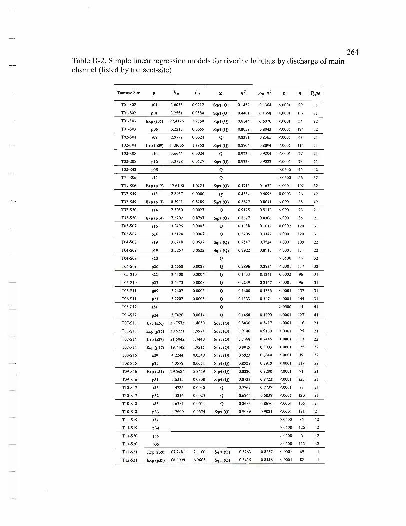
Table D-2. Simple linear regression models for riverine habitats by discharge of main channel (listed by transect-site)
Transect-Site y bob J x
TO I-S02 sOl 3,6033 0,0212 Sqr! (Q)
Sqr! (Q)
0, 1452 0,[364 <,0001 99 31
TO I-S02 pOI 3,2551 0,0584 0.4401 0,4358 <,000 1 132 3 1
TO I-S03 Exp (006) 22,4126 2,7660 Sqr! (Q)
Sqr! (Q)
0,6 144 0,6070 <,000 1 54 22
TO I-S03 p06 3,22 18 0,0655 0,8059 0,8043 <,000 1 124 22
T02-S04 009 2,9772 0,0024 Q
Sqr! (Q)
0.839 1 0,8365 <,000 1 63 2 1
T02-S04 Exp (p09) 11.8065 1.3868 0,8904 0,8894 <,0001 11 4 2 1
T02-S05 810 3,6644 0,0024 Q
Sqr!(Q)
0,9234 0,9204 <,000 1 27 21
T02-S05 plO 3,3898 0,0527 0,9233 0,9222 <,0001 73 21
T02-S48 g05 Q
T3 1-S06 812 Q
T3 1-S06 Exp (pI2) 17,6 190 1.0225 Sqrt(Q) 0,1715
T32-S49 s l3 2,8937 0,0000 Q' 0.4334
T32-S49 Exp (p I3) 8,593 1 0.8289 Sqrt (Q) 0.8627
T32-S50 014 2,5050 0,0027 Q 0,9125
T32-S50 Exp (pI4) 7,3702 0,8797 Sqr! (Q) 0,8327
T03-S07 816 3,2496 0,0005 Q 0,1088
T03-S07 pl6 3,3124 0,0007 Q 0,3205
T04-S08 sl 9 3,6248 0.0537 Sqr! (Q) 0,7547
T04-S08 pl9 3.5267 0,0622 Sqr! (Q) 0.8922
T04-S09 820 Q
T04-S09 p20 3,6568 0,0028 Q 0,2896
T05-S 10 822 3.4100 0,0006 Q 0,1433
T05-S 10 p22 3.4373 0,0008 Q 0,2249
T06-S1 1 g09 3,7407 0,0005 Q 0,1400
T06-S 11 p23 3,7207 0,0006 Q 0, 1533
T06-S 12 s24 Q
T06-S12 p24 3,7426 0,00 14 Q 0.1458
T07-S 13 Exp (026) 26,7572 1.4650 Sqr! (Q) 0,8430
T07-S 13 Exp (p26) 20.522 1 1.9974 Sqr! (Q) 0,9146
T07-S 14 Exp (s27) 21.5042 1.7440 Sqrt(Q) 0,7468
T07-S14 Exp (p27) 19,7142 1.92 15 Sqr! (Q) 0,8019
T08-S15 s29 4,2244 0,0549 Sqr! (Q) 0,6923
T08-S15 p29 4,0572 0,065 1 Sqrt(Q) 0,8928
T09-S16 Exp (s31) 29.5634 5,8459 Sqr! (Q) 0,8220
T09-S16 p31 3,63 15 0,0808 Sqr! (Q) 0,8733
TlO-S I7 s32 4.4785 0,0030 Q 0,7767
Tl O-S I7 p32 4,53 16 0.0025 Q 0,6864
TlO-S I8 833 4,6384 0,003 1 Q 0,8683
TlO-S I8 p33 4,2600 0,0674 Sqr! (Q) 0,9089
T II -S I9
Tl I-S I9
Tl I-S20
Tl I-S20
Tl 2-S2 1
Tl 2-S2 1
s34
p34
835
p35
Exp (539) 67,728 1 7,11 60
Exp (p39) 68,3999 6,9668
Sqr! (Q)
Sqr! (Q)
0,8263
0.8435
>,0500 46 42
>,0500 56
0,1632 <,0001 102
0.4098 0,0003 26
0.86 11 <.0001 85
0,9112 <,000 1 73
0,8306 <,0001 85
0,1012 0,0002 120
0,3147 <,000 1 120
0,7524 <,000 1 109
0.89 13 <,000 1 131
>,0500 44
0,2834 <,000 1 117
0.1341 0,0002 96
0,2167 <,000 1 96
0,1336 <,000 I 137
0, 1474 <,000 1 144
>.0500 15
0,1390 <,000 1 127
0,84 17 <,000 1 116
0,9139 <,000 1 125
0,7445 <.000 I 113
0,8003 <,000 I 125
0,6840 <,000 1 39
0,89 19 <,000 1 117
0,8200 <,0001 91
0,8722 <,000 1 125
0,7737 <,000 1 77
0,6838 <,0001 120
0,8670 <,000 1 106
0,908 1 <,000 1 121
>,0500 85
>,0500 126
>,0500 6
>,0500 113
0,8237 <,000 1 69
0,84 16 <,000 1 82
32
32
42
42
21
21
31
31
22
22
32
32
31
31
31
31
4 1
4 1
21
21
22
22
22
22
21
21
21
21
21
21
12
12
42
42
11
II
264

Table D-2. Simple linear regression models for riverine habitats by discharge of main channel (listed by transect-site) (continuous)
Tl2-S22 (1997)
Tl2-S22 (1997)
Tl2-S22 (1998)
Tl2-S22 (1998)
Tl2-S23
Tl2-S23
Tl3-S24
TI3-S24
Tl 4-S25
Tl4-S25
T15-S26
Tl5-S26
T17-S28
Tl7-S28
Tl8-S29
Tl8-S29
Tl9-S30
Tl9-S30
T20-S31
T20-S3 1
T21-S32
T2 1-S32
T22-S33
T22-S33
T23-S34 ( 1997)
T23 -S34 (1997)
T23 -S34 (1998)
T23 -S34 ( 1998)
T24-S35
T24-S35
T25-S36
T25-S36
T25-S37
T25-S37
T26-S38
T26-S39
T26-S39
T27-S40
T27-S40
T28-S41
T28-S4 1
T28-S42
T28-S42
T29-S43
TJO-S44
538 4.2715 0.0120
p38 4.24 12 0.0142
538 4. 11 51 0.0004
p38 4.1204 0.0005
537
p37 4.2073 0.0300
540 4.1957 0.0519
p40 4.3 653 0.0029
541 4.648 1 0.0372
Exp (p41) 81.5 174 6.4944
Exp (542) 41.0972 2.2279
Exp (p42) 40.5207 2.3996
Exp (551) 32.8971 1.7 194
Exp (pSI) 23 .8867 2.2 115
S54
p54
Sqrt(Q)
Sqrt (Q)
Q
Q
Sqrt (Q)
Sqrt (Q)
Q
Sqrt(Q)
Sqr! (Q)
Sqr! (Q)
Sqr!(Q)
Sqrt (Q)
Sqrt(Q)
0.6367
0.6954
0.11 75
0.1889
0.2 103
0.8955
0.9122
0.6688
0.7840
0.6465
0.6569
0.3425
0.4799
556 4.4980 0.0023 Q 0.9292
p56 4.1610 0.0586 Sqrt (Q) 0.9454
Exp (559) 10.6161 1.644 1 Sqrt (Q) 0.9251
Exp (p59) 11.1 100 1.5802 Sqr! (Q) 0.9182
.60 2.6702 0.0739 Sqrt (Q) 0.9592
Exp (p60) 8.1016 2.3006 Sqrt(Q) 0.9595
568 2.3947 0.0547 Sqr! (Q) 0.927 1
Exp (p68) 8.2805 1.11 54 Sqrt (Q) 0.9437
. 71 3.9038 0.0000 Q' 0.9419
p71 3.4 180 0.06 12 Sqrt(Q) 0.9489
.71 3.8644 0.0034 Q 0.793 1
p71 3.6282 0.0575 Sqrt (Q) 0.927 1
.73 4.2969 0.0023 Q 0.9548
Exp (p73) 36.7697 5.7178 Sqrt(Q) 0.9518
.75 4.5804 0.0459 Sqr! (Q) 0.8560
Exp (p75) 65 .7949 9.0704 Sqrt (Q) 0.9379
Exp (576) 67.0184 9.6238 Sqrt (Q) 0.9467
Exp (p76) 56.7872 10.5410 Sqr! (Q) 0.9589
g26
s78
p78 2.676 1 0.00 18
Exp (s80) 34.6330 0.1095
Exp (p80) 33.6353 0.1133
Exp (s82) 48.5 163 0.0004
p82 3.8276 0.0017
Exp (s83) 45 .5189 2.2966
Exp (p8J ) 42.1458 2.811 4
g29 3.5738 0.00 11
Exp (s87) 28 .2943 1.4580
Q
Q
Q
Q'
Q
Sqrt(Q)
Sqr!(Q)
Q
Sqrt(Q)
0.22 17
0.313 1
0.3087
0.4533
0.4390
0.7410
0.7952
0.3 518
0.2281
0.6249 <.0001 33
0.6856 <.000 I 33
0.0948 0.0283 4 1
0.1681 0.0045 4 1
>.0500 38
0.2030 <.000 1 109
0.8914 <.0001 28
0.9 108 <.000 1 66
0.6625 <.000 1 55
0.78 11 <.000 1 77
0.643 1 <.000 1 106
0.6538 <.0001 113
0.3313 <.000 1 61
0.4749 <.000 1 108
>.0500 74
>.0500 97
0.9258 <.000 1 23
0.9437 <.000 1 34
0.9238 <.000 I 60
0.9 171 <.0001 75
0.9585 <.000 1 64
0.9590 <.000 1 78
0.9260 <.0001 69
0.9429 <.000 1 76
0.9401 <.0001 33
0.9482 <.0001 75
0.7867 <.000 1 34
0.9253 <.0001 42
0.9528 <.0001 25
0.95 14 <.0001 11 3
0.8538 <.000 1 68
0.9373 <.000 1 I I I
0.9458 <.0001 65
0.9584 <.000 1 80
>.0500 96
>.0500
0.2 134 <.000 1 96
0.3050 <.0001 86
0.30 10 <.0001 92
0.4482 <.0001 109
0.434 1 <.000 I 11 6
0.7378 <.0001 84
0.7930 <.0001 95
0.3456 <.000 I 107
0.22 12 <.000 1 114
91
91
91
9 1
41
41
II
II
22
22
22
22
31
31
31
31
2 1
2 1
2 1
21
II
II
11
II
2 1
21
2 1
2 1
21
21
21
2 1
11
11
12
32
32
42
42
12
12
21
21
12
12
265
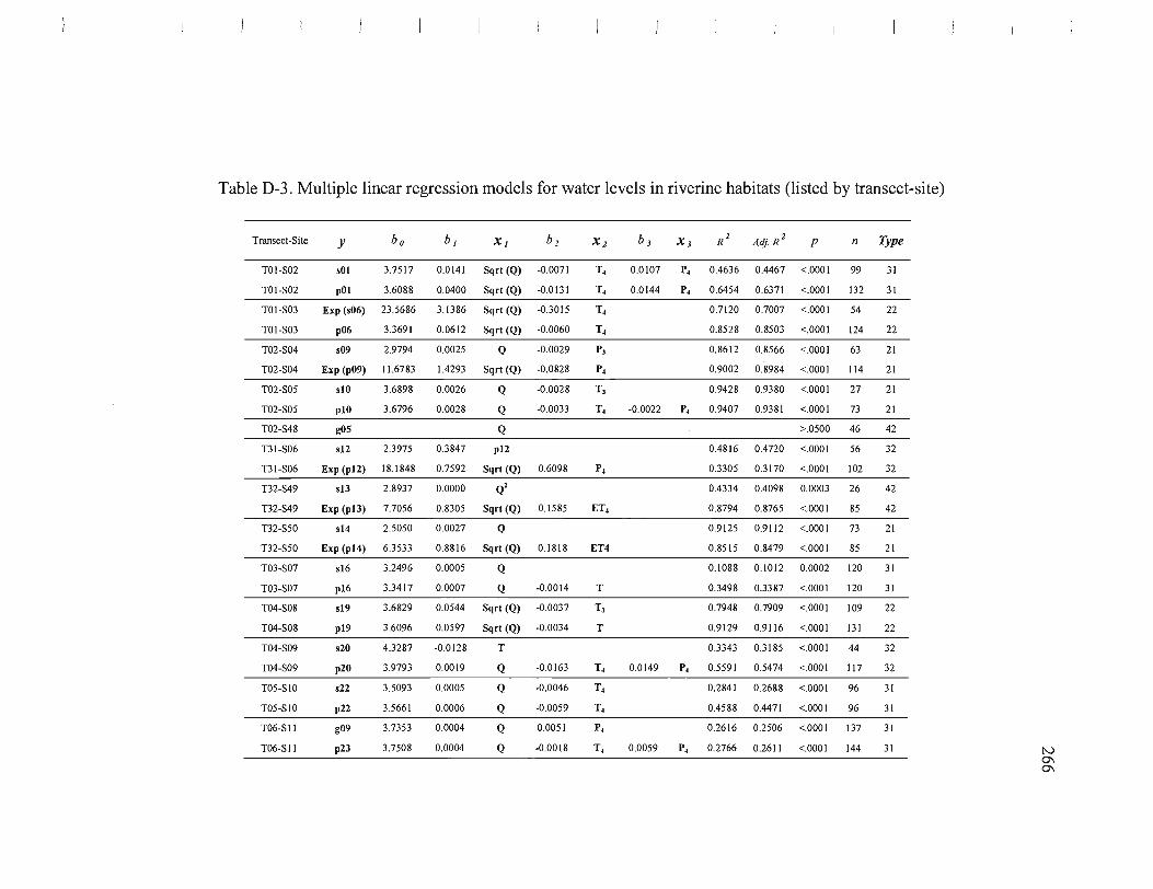
Table D-3. Multiple linear regression models for water levels in riverine habitats (listed by transect-site)
Transect-Site
TOI-S02
TOI-S02
TOI-S03
TOI-S03
T02-S04
T02-S04
T02-S05
T02-S05
T02-S48
T31-S06
T31-S06
T32-S49
T32-S49
T32-S50
T32-S50
T03-S07
T03-S07
T04-S08
T04-S08
T04-S09
T04-S09
T05-S10
T05-SIO
T06-S11
T06-S11
y
sOl
pOl
b o
3.7517
3.6088
b l Xl b 2
0.0141 Sqrt (Q) -0.0071
0.0400 Sqrt (Q) -0.0131
Exp (s06) 23.5686 3.1386 Sqrt (Q) -0.3015
p06 3.3691 0.0612 Sqrt(Q) -0.0060
s09 2.9794 0.0025 Q -0.0029
Exp (p09) 11.6783 1.4293 Sqrt (Q) -0.0828
s10 3.6898 0.0026 Q -0.0028
p10 3.6796 0.0028 Q -0.0033
g05 Q
s12 2.3975 0.3847 p12
Exp (p12) 18.1848 0.7592 Sqrt (Q) 0.6098
s13 2.8937
Exp (p13) 7.7056
s14 2.5050
Exp (p14) 6.3533
s16
p16
s19
p19
s20
p20
s22
p22
g09
p23
3.2496
3.3417
3.6829
3.6096
4.3287
3.9793
3.5093
3.5661
3.7353
3.7508
0.0000 Q2
0.8305 Sqrt(Q) 0.1585
0.0027 Q
0.8816 Sqrt (Q) 0.1818
0.0005 Q
0.0007 Q -0.0014
0.0544 Sqrt (Q) -0.0037
0.0597 Sqrt (Q) -0.0034
-0.0128
0.0019
0.0005
0.0006
0.0004
0.0004
T
Q
Q
Q
Q
Q
-0.0163
-0 .0046
-0 .0059
0.0051
-0.0018
Xl
T,
T,
T,
T,
P3
P,
T3
T,
P,
ET,
ET4
T
T3
T
T,
T,
T,
P,
T,
b 1 Xl R 2 Adj. R 2 P n Type
0.0107 P, 0.4636 0.4467 <.0001 99 31
0.0144 P, 0.6454 0.6371 <.0001 132 31
0.7120 0.7007 <.0001 54
0.8528 0.8503 <.0001 124
0.8612 0.8566 <.000 I 63
0.9002 0.8984 <.0001 114
0.9428 0.9380 <.0001 27
-0.0022 P, 0.9407 0.9381 <.0001 73
>.0500 46
0.4816 0.4720 <.000 I 56
0.3305 0.3170 <.0001 102
0.4334 0.4098 0.0003 26
0.8794 0.8765 <.000 I 85
0.9125 0.9112 <.0001
0.8515 0.8479 <.0001
73
85
0.1088 0.1012 0.0002 120
0.3498 0.3387 <.0001 120
0.7948 0.7909 <.0001 109
0.9129 0.9116 <.0001 131
0.3343 0.3185 <.0001 44
0.0149 P, 0.559 1 0.5474 <.0001 117
0.2841 0.2688 <.000 I 96
0.4588 0.4471 <.0001 96
0.2616 0.2506 <.0001 137
0.0059 P, 0.2766 0.2611 <.0001 144
22
22
21
21
21
21
42
32
32
42
42
21
21
31
31
22
22
32
32
31
31
31
31 N 0\ 0\

Table D-3. Multiple linear regression models for water levels in riverine habitats (listed by transect-site) (Continuous)
T06-S12
T06-S12
T07-S13
T07-S13
T07-S14
T07-S14
T08-S15
T08-S15
T09-S1 6
T09-S16
TlO-SI7
TlO-S17
TlO-SI8
TlO-SI8
TlI-SI9
Tll-S19
Tll -S20
TlI-S20
Tl2-S21
T12-S21
T12-S22 (1997)
T12-S22 (1997)
T12-S22 (1998)
Tl2-S22 (1998)
524
p24 3.9958 -0.0101 T. 0.0133
Exp (526) 28.4952 1.4208 Sqrt (Q) -0.0758
Exp (p26) 22.3388 1.9405 Sqrt (Q) -0.0735
Exp (527) 24.6089 1.6726 Sqrt(Q) -0.1384
Exp(p27) 23 .1596 1.8127 Sqrt(Q) -0.1376
529 4.2339 0.0593 Sqrt (Q) -0.0034
p29 4.1093 0.0635 Sqrt (Q) -0.0018
Exp (s31) 28.2653 6.1459 Sqrt (Q) -0.4800
p31
s32
p32
s33
p33
s34
p34
s35
p35
3.7074
4.5681
4.5941
4.7052
4.3084
0.0812 Sqrt (Q) -0.0034
0.0030 Q -0.0047
0.0026 Q -0.0029
0.0032 Q -0.0036
0.0679 Sqrt (Q) -0.0022
Exp (s39) 58.4352 6.9952 Sqrt (Q) 0.6114
Exp (P39) 57.6750 6.8471 Sqrt (Q) 0.6475
s38 4.3343 0.0109 Sqrt (Q) -0.0028
p38 4.3050 0.0131 Sqrt(Q) 0.0028
s38 4.1906 -0.0027 T
p38 4.1956 -0.0026 T 0.0010
p.
T.
T.
T.
T.
T
T
p.
T
T
T
T
T
p.
p.
T
T
p.
>.0500 15
0.2631 0.2512 <.0001 127
0.8614 0.8589 <.0001 116
0.9227 0.9214 <.0001 125
0.7834 0.7795 <.000 I 113
0.8258 0.8229 <.0001 125
0.7324 0.7175 <.0001 39
-0.0027 P 0.9056 0.9031 <.000 I 117
0.8393 0.8357 <.0001 91
-0.0051 p. 0.8959 0.8933 <.0001 125
-0.0038 PJ 0.8359 0.8292 <.0001 77
-0.0038 p. 0.7229 0.7158 <.0001 120
-0.0029 p. 0.9130 0.9104 <.0001 106
-0.0039 p. 0.9242 0.9223 <.0001 121
>.0500 85
>.0500 126
>.0500 6
>.0500 113
1.5214 ET. 0.8610 0.8545 <.0001 69
1.7696 ET. 0.8769 0.8722 <.0001 82
0.8145 0.8021 <.0001 33
0.8390 0.8283 <.0001 33
0.3688 0.3527 <.0001 41
0.4130 0.3821 <.000 I 41
41
41
21
21
22
22
22
22
21
21
21
21
21
21
12
12
42
42
II
II
91
91
91
91 tv 0\ -.....l

Table D-3. Multiple linear regression models for water levels in riverine habitats (listed by transect-site) (Continuous)
Tl2-S23
T12-S23
T13-S24
T13-S24
T14-S25
Tl4-S25
Tl5-S26
Tl5-S26
T17-S28
Tl7-S28
Tl8-S29
Tl8-S29
Tl9-S30
Tl9-S30
T20-S31
T20-S31
T21-S32
T21-S32
T22-S33
T22-S33
T23-S34 (1997)
T23-S34 (1997)
T23-S34 (1998)
T23-S34 (1998)
4,5247 0,0141 p. s37
p37 4,0929 0,0281 Sqrt (Q) 0,0156
s40
p40
s41
4,1957 0,0519 Sqrt (Q)
4.3653 0,0029 Q
4,6481 0,0372 Sqrt (Q)
Exp (p4I) 80,3737 6.4039 Sqrt (Q) 0,6201
Exp (s42) 45,1162 2,1355 Sqrt (Q) -0 ,1728
Exp (p42) 44,9836 2.2821 Sqrt (Q) -0 ,1848
Exp (s5I) 35.4979
Exp (p5I) 29.4555
1.8539 Sqrt (Q) -0.3085
1.9447 Sqrt (Q) -0,2569
S54
p54
s56
3.5796 -0,0045
3.6441 -0.0099
4,5077 0,0023
T4
T.
Q
p56 4,1610 0,0586 Sqrt (Q)
Exp (s59) 10,6161 1.6441 Sqrt (Q)
Exp (P59) 11.1100 1.5802 Sqrt (Q)
0,0126
0,0143
-0,0031
s60 2,7242 0,0730 Sqrt (Q) -0 ,0024
Exp (P60) 8, I 016 2.3006 Sqrt (Q)
s68 2,3947 0,0547 Sqrt (Q)
Exp (P68) 8.2805 1.1154 Sqrt (Q)
s71 3,9038 0,0000 Q2
p71 3.4180 0,0612 Sqrt (Q)
s71 3,9329 0,0030 Q -0,0025
p71 3,6975 0.0533 Sqrt (Q) -0,0021
p.
p.
T
T
T.
T.
p.
p.
p.
T
T.
T.
0.3013 0.2819 0,0004 38 41
0,0155 ET. 0,3870 0.3695 <,0001 109 41
0.8955 0.8914 <,000 I 28 II
0,9122 0.9108 <,0001 66 I I
0,6688 0,6625 <,000 I 55 22
0,8042 0,7989 <,0001 77 22
0,6717 0.6654 <,0001 106 22
0,6793 0,6735 <,0001 113 22
0.4598 p. 0,5022 0.4760 <,0001 61
0.4724 p. 0.5748 0,5625 <,0001 108
0.4046 0,3878 <,0001 74
0.3299 0,3156 <,0001 97
0,9426 0,9368 <,000 I 23
0,9454 0,9437 <,0001 34
0,9251 0,9238 <,0001 60
0,9182 0,91n <,0001 75
0,9655 0.9644 <.0001 64
0,9595 0,9590 <,0001 78
0,9271 0.9260 <,0001 69
0,9437 0,9429 <,0001 76
0,9419 0.9401 <,0001 33
0,9489 0,9482 <,0001 75
0,8286 0,8175 <,0001 34
0.9341 0,9307 <.0001 42
31
31
31
31
21
21
21
21
II
II
II
II
21
21
21
21 N 0\ 00

Table D-3. Multiple linear regression models for water levels in riverine habitats (listed by transect-site) (Continuous)
T24-S35 573 4.2969 0.0023 Q 0.9548 0.9528 <.0001 25 21
T24-S35 Exp (p73) 36.7697 5.7178 Sqrt (Q) 0.9518 0.9514 <.0001 113 21
T25-S36 575 4.5804 0.0459 Sqrt (Q) 0.8560 0.8538 <.0001 68 21
T25-S36 Exp (p75) 65.7949 9.0704 Sqrt (Q) 0.9379 0.9373 <.0001 II I 21
T25-S37 Exp (576) 67.0184 9.6238 Sqrt (Q) 0.9467 0.9458 <.0001 65 II
T25-S37 Exp (p76) 56.7872 10.5410 Sqrt (Q) 0.9589 0.9584 <.0001 80 \I
T26-S38 g26 >.0500 96 12
T26-S39 578 >.0500 8 32
T26-S39 p78 2.7636 0.0018 Q -0.0050 T .. 0.2663 0.2505 <.0001 96 32
T27-S40 Exp (580) 34.6330 0.1095 Q 0.3131 0.3050 <.0001 86 42
T27-S40 Exp (p80) 33.6353 0.1133 Q 0.3087 0.3010 <.0001 92 42
T28-S41 Exp (582) 47.0490 0.0004 Q2 0.6181 p .. 0.5696 0.5615 <.0001 109 12
T28-S41 p82 3.8276 0.0017 Q 0.4390 0.4341 <.0001 116 12
T28-S42 Exp (583) 48.2730 2.1882 Sqrt (Q) -0.1241 T .. 0.7828 0.7775 <.0001 84 21
T28-S42 Exp (p83) 46.8555 2.5552 Sqrt (Q) -0.1750 T .. 0.8392 0.8357 <.0001 95 21
T29-S43 g29 3.5738 0.0011 Q 0.3518 0.3456 <.0001 107 12
nO-S44 Exp (587) 22.8970 1.4896 Sqrt (Q) 0.8759 ETJ 0.2875 0.2747 <.0001 114 12
nO-S44 Exp (p87) 23.8785 1.4851 Sqrt (Q) 0.7299 ETJ 0.3071 PJ 0.3370 0.3173 <.0001 105 12
nO-S45 Exp (589) 25.5208 2.1387 Sqrt (Q) -1.6446 log (P) 0.8081 0.7879 <.0001 22 81
T30-S45 Exp (p89) 25.4898 2.1389 Sqrt (Q) -1.6198 log (P) 0.8108 0.7909 <.0001 22 81
T30-S46 590 3.5058 0.0026 Q -0.0375 log (P) 0.8894 0.8764 <.0001 20 21
nO-S46 Exp (p90) 14.9481 2.4909 Sqrt (Q) 0.4721 ET .. 0.8324 0.8294 <.0001 115 21
T30-S47 g30 2.8463 0.0938 Sqrt (Q) 0.9302 0.9294 <.0001 84 II
tv 0\ \0


![North Platte Tribune. (North Platte, NE) 1894-11-07 [p ].](https://static.cupdf.com/doc/110x72/6194f7b6b7b4a03a236f33dd/north-platte-tribune-north-platte-ne-1894-11-07-p-.jpg)