1
Repo Haircuts and Economic Capital:
A Theory of Repo Pricing
Wujiang Lou1
1st draft February 2016; Updated June, 2020
Abstract
A repurchase agreement lets investors borrow cash to buy securities. Financier only lends
to securities’ market value after a haircut and charges interest. Repo pricing is characterized with
its puzzling dual pricing measures: repo haircut and repo spread. This article develops a repo
haircut model by designing haircuts to achieve high credit criteria, and identifies economic capital
for repo’s default risk as the main driver of repo pricing. A simple repo spread formula is obtained
that relates spread to haircuts negative linearly. An investor wishing to minimize all-in funding
cost can settle at an optimal combination of haircut and repo rate. The model empirically
reproduces repo haircut hikes concerning asset backed securities during the financial crisis. It
explains tri-party and bilateral repo haircut differences, quantifies shortening tenor’s risk reduction
effect, and sets a limit on excess liquidity intermediating dealers can extract between money
market funds and hedge funds.
Keywords: repo haircut model, repo pricing, repo spread, repo formula, repo pricing puzzle.
JEL Classification: G23, G24, G33
A repurchase agreement (repo) is an everyday securities financing tool that lets investors
borrow cash to fund the purchase or carry of securities by using the securities as collateral. In its
typical transaction form, the borrower of cash or seller sells a security to the lender at an initial
purchase price and agrees to purchase it back at a predetermined repurchase price on a future date.
On the repo maturity date T, the lender (or the buyer) sells the security back to the borrower. The
security’s settlement agent will cross the security and cash on the same day, in an operational mode
of delivery vs payment (DVP) to close the repo trade.
1 The views and opinions expressed herein are the views and opinions of the author, and do not reflect those of his
employer and any of its affiliates.

2
From the lender’s perspective, repo is a secured loan. The initial purchase price is its loan
principal, and the repurchase price is principal paid back plus interest earned on the loan. The
purchase price is often different from the security’s then market value, reflecting a price cushion
the lender has demanded to facilitate risk management. The cushion is expressed in two different
but interchangeable ways. As a discount to the market price, it is a haircut, denoted as h, so that
the initial purchase price is the product of 1 minus haircut and the market price. Denote the market
price of the security per unit as P, the loan amount is (1-h)P with one unit of security as collateral.
The amount of hP is a price cushion or price margin in its formal term. The other way around is
the margin (advance) ratio denoted by η, defined as the ratio of the market price of the collateral
to the loan amount minus 1. Obviously, η=h/(1-h), and, (1-h)*(1+η)=1. When h is small, e.g., 5%,
η is very close to h, 𝜂 =̃ ℎ.
As is a loan, the repurchase agreement bears an interest rate, either explicitly stated in the
transaction document or implied from the difference of final repurchase price and the initial
purchase price. The latter normally associates with one period repo when rate is a fixed number,
and the former involves multiple payment and recalculation periods that necessitate floating rate
resets. We use rp to denote the repo interest rate.
A more accurate characterization of repos is secured margin loans. Margin or margining is
a standard mechanism that maintains the initial cushion against market price fluctuations.
Typically this is a daily process that asks the borrower to post additional collateral when the
security experiences a price decline. Additional collateral could be cash, more shares of the same
security, or other permitted securities. Should the market price increases, reverse margin happens
when the lender returns previously held margins, posts cash, or returns a portion of the purchased
securities in an operation dubbed as free delivery. In the repo market, daily margin is the standard2.
As a margined and secured debt instrument, the borrower becomes the repo issuer. A
corporate debt is priced by debt interest rate or yield. Repo pricing is atypical of conventional debt
instruments, in that haircut also needs to be determined. In fact, repo transaction negotiation covers
simultaneously both the haircut and the repo rate. After initial terms are set, such as the principal
amount or units of the security and the maturity, a trader at a dealer-bank needs to respond with a
2 In the Treasury GC (general collateral) market, intra-day margin could happen, which correlates to the fact that there
is no haircut, i.e., no initial margin to start with.

3
haircut and a repo rate (or spread), when he is approached by end-users or investors for their
financing requests. Traders and investors alike will need pricing models to procced, especially
considering the wide spectrum of different asset classes and repo terms, and the lack of a broadly
available, existing market pricing mechanism3.
This article takes up the question of how a repo transaction is priced, including its haircut
and interest rate. While repo studies have been an intense academic interest, published works are
primarily concerned with understanding repo’s role in the short term wholesale funding market
and its financial stability implications. Some market surveys are starting to touch upon the topic
of repo pricing. At transaction level, there is no known published pricing model that answers this
question.
Treating a repo transaction as a credit product with embedded derivatives in the underlying
security, we set out to build a joint model of counterparty credit spread and collateral security price
dynamics. We combine conventional credit risk management approach with well-industrialized
derivatives pricing approach: the former allows us to establish a target haircut level based on credit
risk measurements such as probability of default (PD), expected loss (EL), or unexpected loss (UL,
also referred to as economic capital, EC), and the latter determines the fair repo rate given the
haircut. This combination leaves room for haircuts to be negotiated with end-users while getting
compensated through the fair repo rate. From the investors’ end, since they will have to finance
the residual or haircut portion of the security market value, the overall funding cost (all-in rate)
offers the investor an optimal opportunity, so that the dual pricing measures of haircut and repo
rate are uniquely determined.
We find that given the existence of haircuts, repo’s principal loss is expected to be very
small, such that conventional credit risk pricing models are not able to produce any meaningful
repo spreads. The very existence of haircuts and the failure of standard credit risk models to explain
repo spreads can be termed a repo pricing puzzle. Recognizing the systemic nature of unhedgeable
and undiversifiable repo losses, we reason that an economic reserve is needed. We introduce a
shadow capital account in the Black-Scholes-Merton option pricing economy that associates to the
value-at-risk of the hedging errors. This shadow account is financed by some agents who
3 Such a market pricing mechanism only exists in the general collateral (GC) Treasury repo market, where haircuts
are zero and market participants bid and ask funding rates in a similar manner to the stock market.

4
warehouse the risk and charge a shadow cost of capital, which then has to be recouped through the
repo return, driving up repo spread. This capital charge component far dominates the traditional
expected loss measure, thus solving the pricing puzzle.
Another contribution of this article is identifying economic capital as the mechanism
through which haircuts and repo pricing are linked. In particular, these dual pricing measures of
the repo pricing can be reduced to economic capital alone, in that the haircuts can be designed to
satisfy certain prescribed EC criteria, while the repo spread is driven by the residual economic
capital after the haircut has been applied. Measured by the expected shortfall (or tail loss), EC is
found to be negatively linear in haircuts. The fair repo spread formula is then approximately linear
in haircut as well.
With a transaction pricing model at hand, we also attempt to explain a number of bilateral
and trilateral repo stylized facts reported in the literature. The model can quantify tri-party and
bilateral repo haircuts differences, show tri-party haircuts’ insensitivity to counterparties, set a
limit on the funding liquidity generated by dealers’ intermediating between collateral rich hedge
funds and cash rich money market funds, and corroborate shortening repo maturity as an effective
way of lending risk aversion in the wholesales funding market.
The rest of the paper is organized as follows. Section 1 conducts a brief literature review
focusing on those more relevant to repo transaction pricing or valuation. Section 2 introduces the
repo haircut model with its main components in credit risk measurement targets, collateral asset
price dynamics, and solution procedures. Section 3 utilizes the haircut model to explain the
difference between bilateral repo haircuts and tri-party repo haircuts, and conducts an empirical
study by replaying the haircut hike on asset backed securities during the 2008 financing crisis.
Section 4 presents the economic capital’s role in the break-even repo rate formula, and synthesizes
repo pricing from its dual measures of haircuts and repo rates. Section 5 provides further discussion
on economic capital. Section 6 concludes.
1. Literature Review
Repo's role in leading to the demise of several major financial institutions and near collapse
of the financial system in 2008 has attracted academic research, regulatory, and industry interests.
Gorton and Metrick (2012) present evidence that repo haircuts increased dramatically in the US
bilateral repo market starting late 2007, especially those concerning securitization products. A run

5
on repo ensured and contributed the crisis. The repo run, however, is not found in the similarly
sized tri-party repo market where the repo haircuts barely moved and repo financing for private
label securitization was of very limited size (Krishnamurthy, Nagel, and Orlov 2014). Copeland,
Martin and Walker (2014) confirm that money market funds (MMF) as the main cash lenders in
the tri-party market tend to shut down lending completely rather than asking for higher haircuts in
times of stress. Lacking sophisticated analytical tools to determine haircuts, MMFs usually sign
up dealer offered haircut schedules. The run in the bilateral market, MMFs' shut down in the tri-
party market, and closure of other short term wholesale funding channels such as asset-backed
commercial paper (ABCP) conduits, hit hard the few most vulnerable dealers including Bear
Stearns and Lehman Brothers, whose subsequent collapses caused systemic distress.
It has since become a contemporary research topic to explain exactly how or why funding
market instability such as a repo run could happen. Brunnermerer and Pederson (2009) takes
haircut as a speculator’s required trading capital, and link market illiquidity defined as the
difference between a security’s market price and its fundamental value directly to the shadow cost
of margin capital. A destabilizing "margin spiral" could develop as the security financier sets
haircut based on his knowledge of the fundamental value, the price volatility, and market liquidity.
Aiming specifically at modeling the repo run, dealers' role as funding intermediaries
between cash rich MMFs and collateral rich hedge funds (HF) has been studied in the market
equilibrium setting. Martin, Skeie and von Thadden (2014) build a dynamic equilibrium model
that exploits tri-party and bilateral repo market microstructures (e.g. tri-party daily unwind) to
explain the difference between tri-party and bilateral repo haircuts and explores market conditions
leading to repo market instability. Infante (2019) focuses on the effect of a dealer default while
facilitating collateral movement and extracting desirable excess funding liquidity in a three agent
economy (from HF to dealer to MMF) through two chained repos (repo rehypothecation).
Assuming that the dealer has zero recovery and the MMF gets to set haircut terms at the extreme
downside risk, a market equilibrium then shows that high risk dealers could succumb more easily
to a run of collateral from HFs than a run of cash from MMFs.
Obviously market equilibrium models do not aim at transaction pricing: coming up with a
repo haircut and repo spread, given a repo trade with a set of terms. Econometric studies could
help, especially those conducted at the transaction level. Krishnamurthy et al (2014) parse MMF
and securities lenders’ SEC quarterly regulatory fillings during the period of January 2007 to June

6
2010. Copeland et al (2014) have access to a Federal Reserve Bank’s daily collected, confidential
tri-party dataset that covers all major tri-party players including dealers and banks, thus a larger
dataset than Krishnamurthy et al. Their data, however, are aggregates at dealer/investor and
collateral type levels, without transaction level details. Hu, Pan and Wang (2019) extract a similar,
but more extensive Tri-party dataset from MMF reports, including trade level repo terms, which
enables the authors to explore collateral concentration’s role in the tri-party repo pricing.
Tri-party repo data and statistics, whilst more readily available, may not bear much
relevance to the more dynamic yet opaque bilateral repo market where less liquid, lower credit
quality bonds are more likely to be accepted. Krishnamurthy et al (2014), for example, report that
during the financial crisis, MMF turned away private label ABS papers, but Copeland et al (2014)
show that such papers are still accepted as tri-party collateral, probably by non-MMF investors
such as banks. Indeed, these private ABS are the focus of a confidential dealer-bank’s bilateral
repo dataset Gorton and Metrick (2012) have gained access to. Bilateral repo trades done by banks
and dealers at the time were not subject to regulatory reporting requirements and as a result there
is a severe lack of available data. Another limited and yet also inaccessible bilateral repo dataset
exists with regard to MBS/ABS, see Auh and Landoni (2016). The data came from a single, large
hedge fund that had under management multi-billion securitization assets, financed with repos
done with many dealer-banks on the street. The dataset contains some trades that funded different
tranches of the same securitization at about the same time, which allows a direct assessment of
credit quality (lower tranches are of poorer credit quality) for the first time.
Recognizing the data deficiency in bilateral repos, the Fed launched a bilateral repo data
collection pilot project in 2015. The dataset includes broker-dealer entities of 9 major US bank
holding companies (BHC), but lasts only a single quarter, is not made public, and may not be
representative of the bilateral repo market4. Breach and King (2018) collect securities financing
data from the Fed’s Senior Credit Officer Opinion Survey, for an eight year post-crisis period on
a broader range of collateral types. They are able to isolate and focus on risky collateral financing
4 Baklanova, Caglio, Cipriani and Copeland (2019) estimate the dataset sheer size accounting for about half of the all
bilateral repos. Typical BHC organizes their banks and securities entities separately, which may have their own repo
desks. The bank side’s repo desk is usually entrusted with deploying the bank’s cash as investment through repo,
while the securities firm’s repo desk handles day-to-day liquidity and securities lending (borrowing securities other
desks want to short.) Baklanova et al show the dominance of treasuries and other liquid government or agency bond
collateral, a sure sign that the dataset comes from liquidity management desks. For example, there are private label
mortgage backed securities (MBS) or ABS collateral. The other half could be more diverse and valuable for the
purposes of studying bilateral repo pricing.

7
between dealers and their clients (rather than interdealers). Their dataset doesn’t seem to contain
transaction level details.
In terms of repo pricing, researchers generally agree that collateral quality, volatility,
counterparty, and market liquidity affect haircuts and repo rates. Tri-party repo haircuts are known
to be lower than bilateral haircuts on the same collateral asset types, some referred to as the haircut
difference puzzle (Copeland et al 2014). Hu et al (2019) finds that neither the tri-party repo
haircuts nor repo spreads are sensitive to dealer borrowers. In the bilateral segment, Auh and
Landoni (2016) show that both repo haircuts and repo spreads increase as collateral quality
deteriorates. Breach and King (2018)’s data also show bilateral repo rates or repo spreads tend to
be stable or move together.
The financial stability of the short term wholesale lending market is a priority to regulatory
bodies. Bank for International Settlements (BIS) Committee on the Global Financial System
conducted a market study (CGFS 2010) on how market participants set credit terms for bilateral
repo style transactions. They find diverse market practice in tightening or relaxing securities
financing terms, including varying haircut levels, shortening repo tenors, altering counterparty
credit limits, restricting collateral asset eligibility, and rejecting certain counterparties. The
Financial Stability Board (FSB) enlisted strengthening oversight and regulation of shadow banking
as a major task and published a final document on the regulatory framework (FSB 2015). The new
framework establishes qualitative and minimal standards for collateral haircuts and governance
structures. Although some of standards could be useful in guiding the design and development of
transaction repo haircut models, they are not model per se.
In the industry, securities financing businesses have been adapting to measures of
reforming the financial system, including supplemental leverage ratio, liquidity coverage ratio
(LCR), and net stable funding ratio (NSFR). In bilateral repos and bilaterally negotiated, tri-party
settled repos for non-government collateral, repo tenors are on average longer than what used to
be pre-crisis; most extend beyond 3 months, often with evergreen features5. Repos with one year
tenor or longer are emerging products for commercial and investment banks and insurance
companies -- net cash investors which treat them as a form of short to median term investments.
5 As an example, a repo is called '4/3/4' evergreen, meaning that the original repo term is 4 months and that with 3
months remaining, it can be extended, i.e., closed out and a new 4 month term repo is entered. If one party does not
agree to the extension, it will run off the remaining 3 months. Popular evergreens include '6/3/6', '9/6/9' and '12/9/12'.
BASEL LCR requires coverage of a 30 calendar day liquidity stress scenario and 1 year time horizon of NSFR.

8
Customized transactions are increasingly popular in what are dubbed as structured repos. In
collateral upgrade trades (or collateral swaps), for example, the parties' haircut differentials drive
the economics of the trades. Dynamic haircuts designed to delever the trades are still rare but not
impossible. Meanwhile, broker/dealers and banks are required to fair value repos placed in the
trading book, with repo counterparty credit risk explicitly measured and managed (BCBS, 2016),
in a way not dissimilar from OTC derivatives. Lengthened tenors, new structured features, and fair
value requirement all necessitate consideration of counterparty credit risk and interaction between
haircuts and borrower credit, the main subject of this research.
To accommodate these developments, a robust modeling capacity of repo transactions
becomes a pressing need, especially given "the absence of a clear understanding of the constitution
of haircuts/initial margins" (Comotto, 2012). Different from the literature surveyed above, our
primary motivation is to provide a pricing model for repo traders and investors as well to price a
repo transaction. The general equilibrium approach does not offer transaction level pricing.
Empirical studies could in theory come up with regression models that allow a transaction to be
priced. Such regression models are obviously limited by the private nature of bilateral repo
transactions, which have made it impossible for large scale data collection and data sharing6.
Second, our focus is repos with non-government securities as collateral. Treasuries repos
have well established market and trading mechanisms that have not only afforded in depth research
efforts but also allowed traders to look up to the market to quote a repo. Repos involving non-
government securities collateral are much less understood, mainly because of their over-the-
counter (OTC) nature. US treasuries’ liquidity is also superior to other collateral. In fact, it is fair
to say that treasuries repos are not so much as debt investment instruments as liquidity products.
Our proposed model does apply to treasuries repos, but its impact is limited, because of the reasons
cited above.
2. Repo Haircut Model
In the financial market, haircut is a discount on the market value of a financial asset when
used as collateral for a financial obligation or debt7. In the early days, stock loan brokers used
6 The data sources cited here are all confidential or proprietary. 7 Ashcraft et al (2010) find a quote that shows taking discount on collateral value long existed 2000 years ago.
9
heavy price discount to withstand stock market meltdowns. Intuitively, a haircut on a stock can be
taken as the worst daily or weekly price decline, depending on how long the financer thinks it will
take to liquidate the stock to recover his loan. According to an industry survey (Comotto 2012),
rules of thump based on market experience and simple price volatility measures, such as a multiple
of price return standard deviations, are popular ways of computing haircuts. As risk management
advances, value-at-risk (VaR) measure has been adopted to arrive at a VaR-based haircut, e.g., the
99% tail loss during a 10 day period over a sufficiently long observation period.
VaR-based haircuts are data-driven. Such an approach is as good as data is, and carries the
usual caveat that history may or may not repeat itself. There are cases when pricing history is
absent, too short, or long enough but yet to have seen a meaningful market stress. Lou (2017)
develops a parametric haircut model by employing a double-exponential jump-diffusion model for
collateral market risk and solving haircuts to target credit risk measurements or credit ratings.
Computational results for main equities, securitization, and corporate bonds show potential for
uses in collateral agreements or situations where counterparty independent haircuts are required,
e.g. for regulatory capital calculations, and collateralization for OTC derivatives.
Strictly speaking, these collateral haircuts are not repo haircuts, because their specification
has not made use of the borrower’s credit. Repo has full recourse to the borrower. A security with
a market price of $100, for example, can be used to collateralize $85 cash loan, subject to 15%
discount or haircut. If the borrower fails to pay back this $85 loan and the market price has dropped
to 80, the lender is $5 short after selling the security at the market. That $5 becomes a claim on the
lender’s estate in the senior unsecured rank.
Like holders of other debt instruments, a repo lender is therefore exposed to the borrower's
default risk. As a secured debt, repo has a limited exposure amount, far less than the full loan
amount. For overnight repos with zero haircut, the exposure is one day price decline. For term
repos (i.e., non-overnight repos), the daily margining mechanism kicks in which keeps the
exposure essentially one (future) day, regardless of the repo tenor. By design, repo has only one
day market risk exposure contingent on borrower default.
Complications do arise from practicalities evidenced by margining procedures and default
settlement provisions embodied in MRA (Master Repo Agreement) or GMRA (the Global Master
Repo Agreement). A grace period of at least a day is given, for example, to allow a counterparty

10
to amend a failed margin call. A party can raise a pricing and margin calculation dispute that the
provisions provide a time window to resolve. In all likelihood, the period from the time when a
party last meets a margin call to the time when collateral asset sales are completed will be more
than one day.
Formally known as a margin period of risk (MPR), this period could cover a number of
events or processes, including collateral valuation, margin calculation, margin call, valuation
dispute and resolution, default notification and default grace period, and finally time to sell
collateral to recover the lent principal and accrued interest. Obviously, a longer MPR directly
increases repo’s exposure. If MPR is zero, repo has no exposure, no risk.
As critical as MPR is to repo’s risk, it is not a number readily available or can be rigidly
derived. Typical MPR ranges from 5 days to 20 days, depending on collateral asset liquidity,
concentration, and contractual factors (Andersen, Pykhtin, and Sokol, 2017). In regulatory risk
capital related works, a 10-day MPR is taken as the standard reference for bilateral OTC
derivatives and security financing transactions. Particularly for tri-party repos, because the third
party custodian standardizes and takes over collateral valuations and certain aspects of default
settlement, the length of MPR is expected to be shorter than that of bilateral repo MPRs.
In our model, MPR is taken as a known input. Repo exposure is based on the negative price
movement during the MPR, assuming margin is perfected maintained at the beginning of the MPR,
and collateral security is sold at the period end market price.
2.1. Repo haircuts as a credit risk mitigation measure
The lender's nominal exposure during the MPR is principal plus accrued and unpaid interest
up to the default event date. For haircut modeling purposes, we assume no lapse between the last
margin date and the default event date, so that the repo exposure in the MPR is flat. Any shortfall
from the sales proceeds to cover the exposure results in an unsecured claim which is pari passu to
the borrower’s senior unsecured obligations and subject to the same recovery process.
Repo-style securities financing transactions are kin to OTC derivatives: they have the same
exemption from the automatic stay in the bankruptcy courts, hold the same unsecured rank, and
are subject to the same provisions on bilateral counterparty credit risk in the regulatory risk capital
11
space (BSBC 2016). To be clear, our haircut model considers borrower’s default risk only, typical
of loan analytics when the lender itself is a going concern. This also aligns with BASEL III’s
standard on counterparty valuation adjustment (CVA).
Suppose a hypothetic bank B and a client C enter a repo transaction, where B lends M(t)
amount of cash to client C on ∆(t) units of collateral security with a price process B(t). In typical
industry jargon, B enters into a reverse repo, while C has a repo.
At a constant haircut h, repo margining ensures M(t)=(1-h)∆(t)B(t), for t<min(T, τ), τ is the
default time of the counterparty and T is repo maturity. Let u be the MPR, a known and fixed time
period, then τ+u is when the security is completely sold. For simplicity, we assume all shares are
sold at time τ+u when the mid market price is B(τ+u).
The actual selling price contains a discount g, 1>g≥0, to the mid, which takes into account
the bid/ask spread or other market liquidity considerations, such as a block size discount or a fire
sale discount. Brunnermerer and Pedersen (2009) define market liquidity as the difference between
security transaction price and its fundamental value, an endogenously generated measure. Here we
treat g as an external input, assessed by traders based on collateral asset market condition. Market
liquidity is commonly cited as a contributing factor to haircut, e.g., Gorton and Metric (2012),
Krishnamurth et al (2014), Copeland et al (2014), Martin et al (2014).
Incorporating the liquidity discount, the sales proceed becomes ∆(τ)B(τ+u)(1-g). Party B’s
residual exposure to party C in the senior unsecured rank is (M(τ)-∆(τ)B(τ+u)(1-g))+. Denote Rc as
C’s recovery rate, Гc(t) C’s default indicator, 1 if τ≤t , 0 otherwise. We write B’s loss process at
time t as follows,
𝐿(𝑡) = 𝐿𝑔𝑑Г𝑐(𝑡)∆𝜏(𝐵𝜏(1 − ℎ) − 𝐵𝜏+𝑢(1 − 𝑔))+
, (1.a)
Or in a differential form,
𝑑𝐿(𝑡) = 𝐿𝑔𝑑(1 − 𝑔)∆𝑡𝐵𝑡 (1−ℎ
1−𝑔−
𝐵𝑡+𝑢
𝐵𝑡)
+
𝑑Г𝑐(𝑡) (1.b)
where 𝐿𝑔𝑑 is the loss given default, applied to reflect the repo's recourse on borrower C. For non-
recourse repos (rare), one can simply set to 1. Obviously, if u=0 and g=0, there is no repo loss.
The loss function reflects the credit enhancement role played by haircutting. Let 𝑦 = 1 −
𝐵𝑡+𝑢
𝐵𝑡 be the price decline. If g=0, Pr(y>h) equals to Pr(L(u)>0). Trivially, there will be no loss, if

12
the price decline is less or equal to h. A first dollar loss will occur only if y>h. h thus provides a
cushion before a loss is incurred. Given a target rating class's probability of default (PD) p0, the
first loss haircut can be written as
ℎ𝑝 = inf {ℎ ∈ 𝑅+: 𝑃𝑟(𝐿(𝑢) > 0) ≤ 𝑝0}. (2)
For rating agencies that employ expected loss (EL) based target per rating class, haircuts
are based on EL target L0,
ℎ𝐸𝐿 = inf {ℎ ∈ 𝑅+: 𝐸[𝐿|ℎ] ≤ 𝐿0}, (3)
L0 can be set based on criteria of certain designated high credit rating, whether bank internal
or external such as Moody’s 'Aa1' rating. Apart from PD and EL, another common measure
adopted in credit risk management is credit value-at-risk (CVaR). Given a quantile q, CVaR is
defined as follows,
𝐶𝑉𝑎𝑅𝐿(ℎ) = inf {𝑙 ∈ 𝑅+: Pr (𝐿(𝑇) > 𝑙|ℎ) ≤ 1 − 𝑞}, (4)
A typical value of q is 99.9% for one year holding period, T=1.
The difference between CVaR and EL is unexpected loss (UL), a reserve capital measure
formally termed economic capital (EC), EC(h)=CVaR(h)-EL(h). The VaR measure is replaced by
expected shortfall (ES) in the newly proposed BASEL market risk capital rules (BCBS, 2016)8,
EC(h)=ES(h)-EL(h). Naturally we can define a haircut to minimize capital requirement C0.
ℎ𝐸𝐶 = inf {ℎ ∈ 𝑅+: 𝐸𝐶(ℎ) ≤ 𝐶0}, (5)
where EC is measured either as CVaR or ES subtracted by EL.
A street firm usually considers and organizes repo business from two different perspectives:
one is liquidity line of operation and the other is lending line business (see also footnote 4).
Treasury repos, especially those with short tenors, generally fall under the liquidity line. These
repos do not earn many basis points above benchmark short term interest rates, such as the Fed
fund rates. The lending line is subject to the firm’s credit risk management practice and policies.
Repo haircuts, treated as a credit risk mitigation tool, require credit department’s approval, often
8 Expected shortfall has yet to make it into the BASEL’s credit risk framework, although researches are under way,
e.g., Osmundsen, Kjartan Kloster, 2018. "Using expected shortfall for credit risk regulation," Journal of International
Financial Markets, Institutions and Money, Elsevier, vol. 57(C), pages 80-93.

13
per transaction. A firm’s credit policy thus must provide a method of deriving a haircut at the
transaction level. In doing so, it may choose a haircut policy. They may choose S&P or equivalent
ratings that are based on controlling probability of loss, e.g., `AA` rating with a PD, p0=0.00005.
Or they can decide on Moody’s or similarly EL based ratings, e.g., `AA` rating with an EL target,
L0=0.0004. Following the financial crisis, banks have developed their own internal rating systems
and have specifications of these PD or EL criteria per rating.
To solve haircuts from equations (2, 3, 4 or 5), the probability distribution of L(T) needs to
be specified, which is governed by the default time model and the collateral price dynamics
provided below.
2.2. Credit Spread and Collateral Price Dynamics
The loss function (equation 1.b) has an exposure amount dependent on a forward put option
on the collateral asset. Since the strike 1−ℎ
1−𝑔 is practically less than 1 as haircut is non-zero, the put
is out-of-the-money. And because the put expiry -- the MPR u – is very short, the value of the put
is predominantly decided by skewness and tail characteristics of the asset return distribution. Asset
price models with stochastic volatility and jumps in both return and volatility are shown to produce
better empirical results in studies of stock indices (Eraker, Johannes and Polson, 2003). Indeed,
stochastic volatility models are welcomed in the options pricing literature and industry practice,
but they are shown to be less effective for very short term options (Eraker 2004).
The double exponential jump-diffusion (DEDJ) model (Kou, 2002) we choose here is
popular in exotic and path dependent options pricing, which allows asymmetric up and down
jumps. A single asset's price process B(t) is written as follows,
𝑋𝑡 = log (𝐵𝑡
𝐵0)
𝑑𝑋𝑡 = 𝜇𝑑𝑡 + 𝜎𝑎𝑑𝑊𝑎(𝑡) + ∑ 𝑌𝑗𝑑𝑁𝑡𝑗=1 (6)
where σa is the asset volatility, µ the asset return, dWa(t) a Brownian motion, dN(t) a Poisson
process with intensity λ, and Yj a random variable denoting the magnitude of the j-th jump. With
DEJD, Yj, j=1, 2, ..., are a sequence of independent and identically distributed double-exponential
random variables with the probability density function (pdf) fY(x) given by

14
𝑓𝑌(𝑥) = 𝑝𝑢𝜂𝑒−𝜂𝑥𝐼{𝑥 ≥ 0} + 𝑞𝑑𝜃𝑒𝜃𝑥𝐼{𝑥 < 0} (7)
where pu and qd are up jump and down jump probabilities, pu+qd=1. The up jump size is
exponentially distributed at a rate of η>1. Similarly θ>0 is down jump’s rate.
The forward put drives the repo’s market exposure which is contingent on the borrower’s
default. In the credit derivatives world, the reduced form model has become the main default
modeling approach. Corporate credit spreads are shown to exhibit log OU (Ornstein-Uhlenbeck)
behavior (Duffie 2011) which is positive, mean-reverting, and highly elastic in that it allows large
moves in credit spread. In the log OU model, the default intensity λc(t) for the default time τ is
written as follows,
𝜆𝑐(𝑡) = e𝑦(𝑡),
𝑑𝑦(𝑡) = 𝑘(�̅� − 𝑦(𝑡))𝑑𝑡 + 𝜎𝑐𝑑𝑊𝑐(𝑡) (8)
where k is the mean reversion rate, �̅� the mean reversion level, σc credit spread volatility, and dWc(t)
a Brownian motion defined in a proper probability space (Ω,Ƒ,P).
The asset price process is correlated with the intensity, <dWc(t), dWa(t)> = ρdt, ρ the
correlation coefficient. dWa can be written in a factor form, 𝑑𝑊𝑎 = 𝜌𝑑𝑊𝑐 + √1 − 𝜌2𝑑𝑊, where
dW is independent of dWc(t). A negative correlation implies that when the credit deteriorates, the
asset return also tends to go down, thus creating a scenario of the “wrong-way risk” (WWR).
The log OU dynamic spread model, while empirically supported, is known for its lack of
analytical tractability. A Monte Carlo simulation is commonly needed. Suppose that we simulate
a path of Wc(t), Ƒc ={Wc(t), 0≤t≤T}. It then leads to a path of y(t), denoted as yF(t). Conditioning
on Ƒc, B(t) has a changed drift term but otherwise remains a DEJD process, as listed below,
𝐵(𝑇)
𝐵(𝑡−)|F𝑐 = 𝑒α(t,T,𝑊𝑐)+σ𝑎√1−𝜌2(W(T)−W(t)) ∏ 𝑒𝑌𝑖
𝑁(𝑇)
𝑖=𝑁(𝑡)
𝑋𝑡(T)|F𝑐 = log (𝐵𝑇
𝐵𝑡−) = α(t, T, W𝑐) + 𝜎𝑎√1 − 𝜌2(𝑊(𝑇) − 𝑊(𝑡)) + ∑ 𝑌𝑗
𝑁𝑇𝑗=𝑁𝑡
α(t, T, W𝑐) = μ(T − t) + σ𝑎ρ(𝑊𝑐(T) − 𝑊𝑐(t)). (9)

15
Fix a time horizon T, the conditional expected loss is
E[L(T)|Ƒ𝑐] = 𝐿𝑔𝑑(1 − 𝑔) ∫ 𝑑𝑃𝑦𝐹(𝑡)𝐸[∆𝑡𝐵𝑡|Ƒ𝑐]𝐸[(
1−ℎ
1−𝑔−
𝐵𝑡+𝑢
𝐵𝑡)
+
|Ƒ𝑐]𝑇
0 (10)
where 𝑃𝑦𝐹 is the conditional default probability, 𝑃𝑦𝐹
(𝑡) = 1 − 𝑒− ∫ 𝑒𝑦𝐹(𝑠)𝑑𝑠 𝑡
0 .
To compute the tail probability of loss at time T exceeding an amount b, Pb=Pr(L(T)≥b),
we again resort to conditioning to arrive at,
𝑃𝑏 = E[I{L(T) ≥ 𝑏}] = 𝐸[E[I{L(T) ≥ 𝑏}|Ƒ𝑐]],
𝐸[I{L(T) ≥ 𝑏}|Ƒ𝑐] = ∫ 𝑑𝑃𝑦𝐹(𝑡)Pr {𝑋𝑡+𝑢 ≤ log (
(1−ℎ)𝐿𝑔𝑑−𝑏
𝑀𝑡
(1−𝑔)𝐿𝑔𝑑) |Ƒ𝑐}
𝑇
0 (11)
where 𝑏 < 𝐿𝑔𝑑(1 − ℎ)∆𝑡𝐵𝑡 . 𝑏
𝑀𝑡 is the relative loss measured against the repo principal 𝑀𝑡 =
(1 − ℎ)∆𝑡𝐵𝑡, and Pr{.} is the cumulative density function (cdf) of Xt.
Repo style security financing transactions operate either with fixed positions where ∆(t) is
constant or constant exposure where ∆(t)B(t) is constant. The latter corresponds to a constant loan
amount M0, which is the norm in repo. The former is typical of a sec lending or total return swap
(TRS) funding transaction9. Since our focus is repo, we can take out 𝐸[∆𝑡𝐵𝑡|Ƒ𝑐] in equation (10)
to normalize the loss as the percentage of the loan. Accordingly, in the remaining text, we assume
Mt=M0=1, a unit notional.
2.3. Negative linear VaR and ES in haircuts
The conditional expectation 𝐸[(1−ℎ
1−𝑔−
𝐵𝑡+𝑢
𝐵𝑡)
+
] in equation (10) is evaluated by inverse
Laplace transform (Cai, Kou, and Liu, 2014), so is cdf of Xt for equation (11). Pb is then obtained
9 As far as the margin account is concerned, the latter is equivalent to the use of the same collateral to fund the margin
account, which alternatively could be funded with cash or government debts. This has a negative leveraging effect
when B's price declines. Some may consider introducing price floors to limit the extent of this leverage for certain
high volatility asset classes. In the simulation model, this is relatively straightforward to capture and will be left for
future exercises.

16
by running a Monte Carlo (MC) simulation on equation (11). EL is obtained similarly from
simulating equation (10). Zero correlation is a special case where equations (10 & 11) can be
evaluated without the need of running MC simulation, once the default probability 𝑃𝑦 is
computed separately.
Obviously Pb depends on h, better written as 𝑃𝑏|ℎ. Fixing a haircut h, equation (11) gives
loss distribution Pb as a function of b. We set up a loss grid in b with step size Δb, b0=0, b1, b2, …,
bI, and bi =iΔb. For each bi, Pb|h becomes a function of h. In particular, for b0=0, the no loss
probability P0|h can be inverted to solve for h given a target level of P0 for a given PD based rating
class.
It is useful for implementations to note that equation (11) is translational in h and b, i.e.,
𝑃𝑏∗|ℎ∗ = 𝑃𝑏|ℎ,
𝑏∗ = 𝑏 + (ℎ − ℎ∗)𝐿𝑔𝑑 (12)
An implementation could start with h=0, choose Δb=𝐿𝑔𝑑Δh, compute 𝑃𝑏|ℎ on the loss grid
bi. Then on a haircut grid, h*=iΔh, i=0, 1,2, …, I, use equation (12) directly to look up 𝑃𝑏∗|ℎ∗.
For a fixed h, VaRL can be solved by finding b such that Pb|h=1-q, loss not exceeding b
with the confidence interval q. For a different haircut h*, we then have 𝑃𝑏∗|ℎ∗ = 1 − 𝑞, so long as
b* is determined by (12). This states that b* is the VaR(h*), if b is VaR(h). Equation (12) gives
𝑉𝑎𝑅(ℎ∗) = 𝑉𝑎𝑅(ℎ) + 𝐿𝑔𝑑(ℎ − ℎ∗) (12.b)
With a sufficiently large haircut, VaRL(h) (equation 4) could be zero, when P0 ≥q. (12.b)
can be refined,
𝑉𝑎𝑅(ℎ∗) =𝑉𝑎𝑅(0) − 𝐿𝑔𝑑ℎ∗, 𝑖𝑓 𝑉𝑎𝑅(0) > 0 𝑎𝑛𝑑 ℎ∗ <
𝑉𝑎𝑅(0)
𝐿𝑔𝑑
0, 𝑒𝑙𝑠𝑒 (12.c)
Therefore, for a meaningful combination of q and h, non-zero VaR of the repo loss
decreases linearly as haircut increases. This is not surprising at all, since haircut directly cuts down
loss and has the effect of truncating the loss distribution.

17
Similarly with b fixed, E[L(T)] can be computed as a function of h to solve for haircut by
definition (equation 3). In particular, there is also a translational formula10 for the (conditional) tail
loss expectation,
𝐸[𝐿ℎ(𝑇)|𝐿ℎ(𝑇) ≥ 𝑏] =𝐸[𝐿ℎ∗(𝑇)]
𝑃[𝐿ℎ(𝑇)≥𝑏]+ 𝑏, (13)
ℎ∗ = ℎ +𝑏
𝐿𝑔𝑑.
where we have added subscript h to the loss function L to denote its association with haircut h as
defined in equation (1). Setting b to VaR(h) (so that 𝑃[𝐿ℎ(𝑇) ≥ 𝑏] = 1 − 𝑞) leads to a convenient
formula that computes ES given a q-tile,
𝐸𝑆ℎ∗ =𝐸[𝐿ℎ𝑞
(𝑇)]
1−𝑞+ 𝑉𝑎𝑅(ℎ∗) (14)
ℎ𝑞 = ℎ∗ +𝑉𝑎𝑅(ℎ∗)
𝐿𝑔𝑑
Plugging (12.c) into (14) to arrive at,
𝐸𝑆ℎ∗ =𝐸[𝐿ℎ𝑞
(𝑇)]
1−𝑞+ 𝑉𝑎𝑅(0) − 𝐿𝑔𝑑ℎ∗ (14.b)
The same negative linear term in haircut seen in (12.c) now appears in the expected
shortfall. This negative linear relationship does not exist in probability of no loss and expected
loss, the other two popular measures of credit risk. VaR and ES thus have a unique advantage in
repo haircut design.
To compute ES given q and an h*, first use (12.c) to get 𝑉𝑎𝑅(ℎ∗), hq from (14), 𝐸[𝐿ℎ𝑞(𝑇)],
then (14.b) to get ES. ES can of course be computed from the discrete loss distribution obtained
from equation (11). Since it depends on the tail of the distribution, its accuracy would require a
very fine loss grid bi, but equation (14.b) allows us to circumvent that.
Cai, Kou, and Liu (2014) develops an inverse transform algorithm with both discretization
and truncation error controls to promote numerical stability. The controls are separately computed
for cdf and options. For our purposes, such an inverse transform is run per path and it will be more
efficient to apply the same transform setting to obtain cdf of Xt. Lou (2017) revises error controls
so that the same truncation and discretization parameters apply to the inversions of cdf and put
10 See Appendix A for derivation.

18
options. DEDJ model estimations conducted on US main equity index, securitized products, and
US corporate bond indices over a 10 year span show reasonable model stability and behavior.
The model discussed above in principal works for securities lending transactions. A sec
lender has a loss on the other side of price movement, i.e., when price appreciation over the MPR
exceeds the extra margin of hBt posted by the security borrower. Expected loss of the sec lender
would then relate to a call option payoff on a constant unit of the collateral security. This would
be left for future research.
3. Predicting Repo Haircuts
A haircut model’s primary application is to predict repo haircuts in accordance with a
bank’s securities financing business model and risk management capacity. If the bank treats the
repo as a secured loan to be carried on its banking book, it then needs to set the haircut that
produces the firm's desired lending profile on a wholesale exposure. Take for example, suppose
the firm is comfortable lending out to 'A' rated wholesale clients unsecured, it could trade a reverse
repo with a 'BB' rated party, provided that the trade has a haircut designed to make the overall
credit risk profile matching that of 'A' rated counterparties.
3.1. US Treasury haircuts
The US Treasury securities are the single most dominant collateral in the repo market.
Table 1 shows 1 day, 5 day, and 10 day VaR and ES market risk measures taken over a 5 year
period from 3/7/2006 to 3/7/2011 with the financial crisis in the middle, and another 5 year period
ending in May 2020 when the coronavirus roiled the market in Q1 2020. One day VaR-based
haircuts for active 10 year notes and 30 year bonds are 1.41% and 2.60% respectively. If one adopts
a MPR of 5 days, notes haircut is 2.9% and bonds 5.22%11.
These data driven, VaR-based haircuts can be complimented by a parametric haircut model.
Estimated DEJD for the current 10 year notes price time series has (μ, σa, λu, λd, ηu, ηd) = (-0.014575,
11 These numbers are surprisingly consistent to typical ISDA Credit Support Annex (CSA) valuation percentages
applied to Treasury notes and bonds, 98% and 95%, which imply 2% and 5% haircuts.

19
0.071804, 27.551, 22.746, 186.42, 232.44) and produces 0.3507 in skewness and 6.1927 in
kurtosis, comparing to sample skewness of 0.1532 and kurtosis of 6.4770.
Table 1. VaR (99 percentile Value-at-Risk) and ES (97.5-percentile Expected Shortfall) during two 5 year
periods containing the 2008 financial crisis and current coronavirus market distress.
Active 5y Notes Active 10y Notes Active 30y Bonds
period/days VaR ES VaR ES VaR ES
2008-1d 0.89 0.91 1.41 1.45 2.60 2.68
2008-5d 1.64 1.70 2.90 2.92 5.22 5.45
2008-10d 2.06 2.11 3.69 3.67 7.79 7.42
2020-1d 0.49 0.51 0.93 1.08 2.16 2.64
2020-5d 1.06 1.08 2.14 2.26 4.97 5.47
2020-10d 1.59 1.52 2.72 2.88 6.96 6.37
Figure 1 shows predicted collateral haircuts targeting Moody's and S&P investment grade
(IG) credit ratings, i.e., hEL and hp. The hypothetic S&P ‘A’ and above rating targeted haircuts are
about 1~2 points higher than corresponding Moody's rating targeted haircuts. Caution should be
taken, however, these default rates and loss rates are examples and not directly comparable against
each other. A firm may choose one haircut policy, e.g., designing haircuts to match an overall ‘AA’
Moody’s rating or some internal credit rating criteria, with the understanding that different rating
criteria does lead to some variations in haircut levels, as shown here. We also show hEC or hES (as
ES is used as EC), which produces haircuts somewhat in the middle of Moody’s and S&P’s rating
haircuts.
Numbers shown in Figure 1 are collateral haircut, i.e., counterparty independent haircuts.
Among the money market fund families’ tri-party repos, Treasury haircuts are in a very tight range
around 2% (Tables 9 and 10 in Hu et al 2019), with a mean remaining maturity of 6.21 years, and
notes on average accounting for 79%. Top ten dealers’ mean haircuts range from 1.97% to 2.10%,
and the standard deviations range from 0.14% to 0.52%. These ranges overlap closely with the
above one and 5 day VaR-based collateral haircut range of 1.4% and 2.9%. This makes it difficult
to tell whether MMFs are using collateral haircuts for their Treasury repos or they price repo
haircuts in a tight range because the dealers’ credit quality are in a tight range. We will have to
look at more volatile collateral asset classes.

20
Figure 1. Predicted Treasury notes haircuts (MPR 5 days) targeting hypothetical Moody’s one year
loss rates per Bielecki (2008), S&P’s average one year default rates (Standard & Poor’s
2015)12, and EC-based haircuts.
3.2. Equity repo haircuts
Next we consider a bank lends to an 'A' rated wholesale counterparty, for 1 year with US
main equities as collateral13. The asset model is estimated with a 5 year historical period from
1/2/2008 to 1/2/2013. The borrower's spread dynamics is assumed to have 90 bp initial and mean
hazard rate levels, mean reversion speed of 0.5, and spread log OU volatility of 1.50, i.e., k=0.5,
�̅� =log(0.009), σc=1.5, λ0=0.009 in equation (6), such that its 5 year CDS prices at 125 bp14.
The EL based haircut targeting Moody's 'Aa2' without giving consideration to the
borrower's credit is 15.53% (of collateral haircut) for an MPR of 10 days. With borrower's default
probability considered, 7.98% (Table 2) suffices to reach the same 'Aa2' profile under zero credit
and asset correlation. If the correlation is stressed to -0.9, indicative of negative price return
12 Note that the default rates are an average of the global corporate default experience between years 1981 to 2014,
not necessarily same as S&P's calibrated and official default rates. 13 Repo on main equity index has gained popularity recently on top of hedge funds’ equity financing needs from their
prime brokers and/or dealer banks. Bloomberg reports that Soc Gen created a new equity repo strategy to allow
investors to gain on equity index repo rate movements, see https://finadium.com/bloomberg-socgen-marketing-quant-
equity-repo-index-strategy/. 14 Currently 'A' rated corporates have an average 5 year CDS at about 125 bp. This level obviously does not apply in
a credit contraction cycle.
0
1
2
3
4
5
6
7
AAA AA+ AA AA- A+ A A-
Hai
rcu
t (%
)
Ratings
Moody's ES S&P

21
accompanied by worsening credit spread (thus wrong-way risk, WWR), haircut only increases
mildly by 1.13%. Last column of the table shows that haircut changes are negative when the
correlation moves to 0.9, indicating right way risk.
Table 2. Haircuts for hypothetically 'A', 'BBB', 'BB', and 'B' rated borrowers. DEJD model estimated to 2008-2013
data (Est-1: (μ, σ, λ, p, ηu, ηd) = (0.1231, 0.2399, 79.7697, 0.4596, 169.96, 128.36), Lou 2017), target
equivalent wholesale credit rating of 'Aa2', under assumed correlation between equity return and credit spread,
and stress market liquidity discounts.
Borrower
CDS Rating
haircut
rho 0
hc change
rho -0.9
hc change
rho -0.9, g 2%
hc change rho
0.9
125 A 7.98 1.13 1.78 -1.27
250 BBB 9.43 1.11 1.75 -1.25
500 BB 10.85 1.09 1.73 -1.23
1000 B 12.31 1.07 1.7 -1.19
The moderate correlation effect is anticipated as the haircut truncated loss exposure lies in
the tail of asset returns where the Gaussian component of the asset dynamics is not expected to
have a significant impact. Take for example, if the spread volatility is doubled, while keeping the
CDS spread at 250, the haircut for a BBB client would increase 0.38% under -0.9 correlation. The
general wrong way risk therefore is limited, obviously due to the short MPR and the loss buffer
afforded by haircuts.
Specific wrong way risk could occur, if a borrower posts its affiliates' debt instruments as
collateral. A structural dependency stronger than the diffusion correlation between asset return and
credit spread could be developed. The strongest one in fact is a down jump upon borrower default,
which can be modeled as an additional liquidation discount added to g. Specific WWR with a 2%
asset jump on borrower default has a further increase of haircut of 1.78% (fifth column in Table
2). In this sense, specific WWR is very severe, but the real magnitude will be firm and product
dependent, and is best to be analyzed on a case-by-case basis.
Evident from Table 2, haircuts become a tool of credit enhancement to the borrower. A
‘BB’ rated client entering a repo, for example, can post additional 1.42% (=10.85%-9.43%)
haircut to make himself a 'BBB' equivalent borrower with the same collateral, both trades showing

22
out an equivalent top credit risk profile of 'Aa2'. For 'BBB', 'BB', and 'B' rated borrowers in the
table, the mean reversion speed and spread volatility are kept same but the initial hazard rates are
set at 2%, 4.88% and 14.3% to produce 5 year CDS spreads of 250, 500, and 1000 bp respectively15.
The stylized fact that MMFs are counterparty insensitive when lending to dealers
(Krishnamurthy et al 2014, and Hu et al 2019) can be readily explained. Noting that most dealer-
banks normally fall into the rating band of 'BBB' and 'A', the separation between 'A' and 'BBB'
rated borrowers is small, about 1.45% in haircut. This is not enough a margin for unsophisticated
MMFs to invest in their risk management capacities. As a result, in times of stress or crisis, they
would opt to other means to restrict lending money to dealer banks, such as shortening repo tenor,
reducing lending amount or ultimately shutting down (Comotto, 2012).
In the results presented above, a one-year repo tenor is assumed, as wholesale credit risk
management typically standardizes around senior unsecured exposure at one year time horizon.
For trades of longer or shorter terms, one can convert it to an equivalent one year credit risk profile
to allow comparisons with a firm’s internal credit risk metrics to define haircut targets. Or one
could scale the standard one year loss or default rate to the tenor in question based on piecewise
constant hazard rates.
Similar collateral haircut tables can be developed for corporates, CMBS, RMBS, and ABS,
with proper proxy indices identified and the jump-diffusion model estimated. Results are omitted.
3.3. Tri-party and Bilateral Repo Haircut Difference Puzzle
Gorton and Metrick (2012) show dramatic increases of bilateral haircuts during the crisis,
while tri-party repo datasets (Krishnamurthy et al, 2014, and Copeland et al, 2014) show mostly
stable haircuts. The abnormally large difference in tri-party and bilateral haircuts, e.g., about 15%
for private label MBS prior to Lehman's default and about 30% post default, is not apparent
economically. Krishnamurthy et al (2014) attribute the rise of haircuts in the bilateral markets to
a credit crunch on the part of the dealers, while Copeland et al (2014) leave it as an open haircut
difference puzzle. Martin et al (2014) recognize contributions from different institutional
15 These are for illustrative purposes only. An implementation should estimate or calibrate these parameters from
single name CDS or properly chosen CDS indices.

23
arrangements in that bilateral trades are more custom negotiated, whereas tri-party terms are more
template based thus more standardized.
Our transaction oriented haircut model offers an explanation of the puzzle from the
borrower credit perspective. Dealers as borrowers of cash are generally of much better credit
quality than HFs. By looking up from Table 2, if we assume the dealer is 'A' rated, the MMF would
charge a haircut of 7.98%. The dealer would charge a 'BB' rated HF 10.85%, assuming zero
correlation.
Rating HFs is a very difficult task. Small HFs are highly concentrated in an asset class or
a particular kind of investment strategies, so that severe asset valuation distress could threaten the
very survival of the fund, an extreme case of significant or specific wrong way risk. Large or multi-
strategy HFs organize investment around sub-funds, each of which either pursues a specific
strategy or is managed by a portfolio manager (PM). Investment performance is measured at the
sub-fund level and investors can choose sub-funds to invest. Sub-funds operate under the parent
company’s legal umbrella, and as a result they can’t be the legal borrowing entity in a repo
transaction. But because their investment money and management team are segregated, their use
of leverage has to be segregated as well. Repo with a HF is therefore structured to eliminate any
credit support from the parent fund. In that sense, it is prudent to apply collateral haircut of 15.53%,
resulting in a haircut difference of 7.55%.
Another factor contributing to the difference is the length of the MPR. In the tri-party
market the MPR is shorter, because of its institutional efficiency in collateral valuation and
settlement (Copeland, Duffie, Martin, and McLaughlin 2012). In the bilateral market, the MPR is
generally longer due to trade customization, valuation dispute, and other bilaterally negotiated
terms that could prolong the settlement process. Valuation dispute alone may take up to 3 days to
resolve. With our model, longer MPR leads to higher haircut. To illustrate, if the MPR drops from
10 days to 5 days, the MMF haircut or tri-party haircut would reduce from 7.98% to 5.34%,
widening the haircut difference by 2.64%, to a final number of 10.19%.
Haircut difference between bank and HF counterparties is also evident in Gorton and
Metrick (2012)'s bilateral repo dataset, where interdealer bilateral haircuts are compared side by
side on the same collateral class with bilateral haircuts facing mid-sized hedge funds ($2-5 billion
asset under management), as seen from Table 1 in Dang et al (2013). For BBB+/A rated corporate
bonds in Jan 2009, for instance, the bilateral haircuts are 0-5% with banks and 35%-40% with HFs,

24
thus a bank-HF difference of at least 30%. In Jan 2007, the bank-HF difference is much smaller,
at about 10%.
3.4. Dealer’s intermediating liquidity
This bilateral and tri-party haircut difference, if utilized by an intermediating dealer,
generates excess cash liquidity. A dealer, for example, can fund its HF client $84.47 on $100
security with 15.53% haircut, and gets funded $94.66 by rehypothecating the security to an MMF
at 5.34% haircut, realizing $10.19 of excess liquidity.
With an analytic model at hand, an upper bound for the excess liquidity can be established.
For the first leg where the dealer gets funded by an MMF, the lending MMF would demand a
haircut hMMF with the dealer as the counterparty. On the second leg the dealer lends to a HF which
can be thought as a counterparty of not much credit worthiness beyond what the collateral asset
can afford. In this case, the asset only collateral haircut applies and establishes an up limit of the
haircut differential. Table 3 shows the limit for main equities, where hMMF is set to target Moody's
'Aa2' rating with 5 day MPR while the bilateral haircut targets the same rating although at 10 day
MPR. Obviously in the setup, the excess liquidity or the haircut differential shown in column 'hc
diff' decreases as the CDS spread of the dealer increases, i.e., better credits earn higher excess
liquidity.
The excess liquidity could be greater for securitized products, due to higher asset volatility
and poorer market liquidity. Comparisons of private label CMO haircuts between triparty and
bilateral repo therefore need to be understood with data granularity issues in mind16.
Note that our computed tri-party haircuts and bilateral haircuts are results of applying the
same model to two back-to-back repo trades where the dealer bank is defaultable only when it acts
as a borrower. Infante (2019) has a defaultable intermediating dealer in both trades, in order to
study an excess liquidity chasing dealer’s default impact on the short term funding market. While
a broker-dealer default could be a real concern especially during a financial crisis, day-to-day repo
transactions have to consider borrower default simply because repo is a credit product.
16 Usually the triparty repo market finances higher rated private label CMO tranches while the bilateral market have
higher percentage of lower rated tranches. Gorton and Metrick (2012) show a rating split of ABS/RMBS/CMBS
products into 'AA-AAA' and '<AA', while Krishnamurthy et al (2014) and Copeland et al (2014) have no comparable
rating subclass. CMO tranching directly affects haircuts. In Jan 2007 for example, haircuts collected from HFs are 3%
for 'AAA' rated ABS papers and 25% for 'BB' rated papers (Table 1 in Dang et al 2013).
25
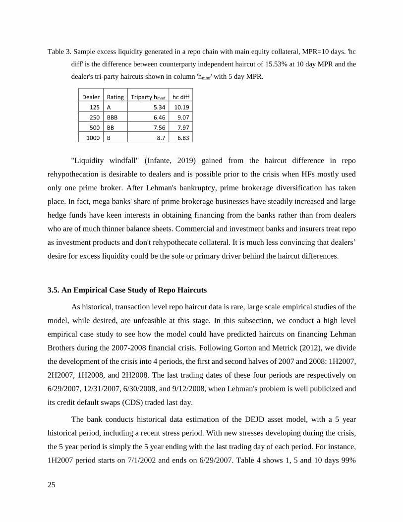
Table 3. Sample excess liquidity generated in a repo chain with main equity collateral, MPR=10 days. 'hc
diff' is the difference between counterparty independent haircut of 15.53% at 10 day MPR and the
dealer's tri-party haircuts shown in column 'hmmf' with 5 day MPR.
Dealer Rating Triparty hmmf hc diff
125 A 5.34 10.19
250 BBB 6.46 9.07
500 BB 7.56 7.97
1000 B 8.7 6.83
"Liquidity windfall" (Infante, 2019) gained from the haircut difference in repo
rehypothecation is desirable to dealers and is possible prior to the crisis when HFs mostly used
only one prime broker. After Lehman's bankruptcy, prime brokerage diversification has taken
place. In fact, mega banks' share of prime brokerage businesses have steadily increased and large
hedge funds have keen interests in obtaining financing from the banks rather than from dealers
who are of much thinner balance sheets. Commercial and investment banks and insurers treat repo
as investment products and don't rehypothecate collateral. It is much less convincing that dealers’
desire for excess liquidity could be the sole or primary driver behind the haircut differences.
3.5. An Empirical Case Study of Repo Haircuts
As historical, transaction level repo haircut data is rare, large scale empirical studies of the
model, while desired, are unfeasible at this stage. In this subsection, we conduct a high level
empirical case study to see how the model could have predicted haircuts on financing Lehman
Brothers during the 2007-2008 financial crisis. Following Gorton and Metrick (2012), we divide
the development of the crisis into 4 periods, the first and second halves of 2007 and 2008: 1H2007,
2H2007, 1H2008, and 2H2008. The last trading dates of these four periods are respectively on
6/29/2007, 12/31/2007, 6/30/2008, and 9/12/2008, when Lehman's problem is well publicized and
its credit default swaps (CDS) traded last day.
The bank conducts historical data estimation of the DEJD asset model, with a 5 year
historical period, including a recent stress period. With new stresses developing during the crisis,
the 5 year period is simply the 5 year ending with the last trading day of each period. For instance,
1H2007 period starts on 7/1/2002 and ends on 6/29/2007. Table 4 shows 1, 5 and 10 days 99%

26
VaR directly estimated from the Bank of America Merrill Lynch's 5 to 10 year average life CMBS
'AA' price return time series. The 10 day VaR doubled from 2H2007 to 1H2008, then nearly
quadrupled from 1H2008 to 2H2008.
Having estimated the asset model, the bank considers both the risk neutral log OU model
-- fitted to the CDS market on a specific trading day, and the real world model estimated from
historical daily CDS curves. Since repo tenors are short, one year in this exercise, there is no need
to fit or estimate the full term structure of Lehman's credit curve. For our purposes, we pick the
historical 1y CDS spread to regress to estimate the log OU model and bootstrap a default
probability curve using only Lehman's 6 month, 1 year and 2 year CDS spreads, which are shown
in Table 5 for the last trading days of the four crisis periods. The need for a logarithm model is
evident from the multiplying jumps seen in these periods.
Table 4. CMBS ‘AA’ 5 to 10 year average life bond 99% VaR estimated with 5 year historical price return data up to
1st half of 2007, 2nd half of 2007, 1st half of 2008, and 2nd half of 2008, for MPRs of 1, 5 and 10 days.
Sharp increases in VaR are observed from 2H2007 to 2H2008.
VaR(%) 1-d 5-d 10-d
1H2007 0.88 1.97 2.9
2H2007 1.05 2.14 3.02
1H2008 1.51 3.71 6.54
2H2008 3.26 9.81 23.49
Table 5. Lehman Brothers’ short term CDS spreads as of the last trading date of the four cited periods.
PeriodEnding 6m 1y 2y
1H2007 0.08% 0.13% 0.19%
2H2007 1.52% 1.44% 1.41%
1H2008 4.43% 4.46% 3.87%
2H2008 14.13% 13.69% 10.09%
The estimated log OU model parameters are listed in Table 6. The estimated volatility is
quite stable but the mean reversion parameter k becomes negative for 1H2008 and 2H2008,
indicating an explosive rather than mean-reverting spread behavior as the broker struggled along
the way to final default (yet still a surprise given its 6 month CDS spread is only 14.13%).
27
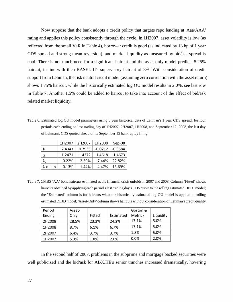
Now suppose that the bank adopts a credit policy that targets repo lending at 'Aaa/AAA'
rating and applies this policy consistently through the cycle. In 1H2007, asset volatility is low (as
reflected from the small VaR in Table 4), borrower credit is good (as indicated by 13 bp of 1 year
CDS spread and strong mean reversion), and market liquidity as measured by bid/ask spread is
cool. There is not much need for a significant haircut and the asset-only model predicts 5.25%
haircut, in line with then BASEL II's supervisory haircut of 8%. With consideration of credit
support from Lehman, the risk neutral credit model (assuming zero correlation with the asset return)
shows 1.75% haircut, while the historically estimated log OU model results in 2.0%, see last row
in Table 7. Another 1.5% could be added to haircut to take into account of the effect of bid/ask
related market liquidity.
Table 6. Estimated log OU model parameters using 5 year historical data of Lehman's 1 year CDS spread, for four
periods each ending on last trading day of 1H2007, 2H2007, 1H2008, and September 12, 2008, the last day
of Lehman's CDS quoted ahead of its September 15 bankruptcy filing.
1H2007 2H2007 1H2008 Sep-08
K 2.4343 0.7935 -0.0212 -0.3584
1.2471 1.4272 1.4618 1.4673
λ0 0.22% 2.39% 7.44% 22.82%
λ-mean 0.13% 1.44% 4.47% 13.69%
Table 7. CMBS ‘AA’ bond haircuts estimated as the financial crisis unfolds in 2007 and 2008. Column "Fitted" shows
haircuts obtained by applying each period's last trading day's CDS curve to the rolling estimated DEDJ model;
the "Estimated" column is for haircuts when the historically estimated log OU model is applied to rolling
estimated DEJD model; 'Asset-Only' column shows haircuts without consideration of Lehman's credit quality.
Period Ending
Asset-Only Fitted Estimated
Gorton & Metrick
Liquidity
2H2008 28.5% 23.2% 24.2% 17.1% 5.0%
1H2008 8.7% 6.1% 6.7% 17.1% 5.0%
2H2007 6.4% 3.7% 3.7% 1.8% 5.0%
1H2007 5.3% 1.8% 2.0% 0.0% 2.0%
In the second half of 2007, problems in the subprime and mortgage backed securities were
well publicized and the bid/ask for ABX.HE's senior tranches increased dramatically, hovering

28
around 5%17. At the end of 2H2007, the predicted haircuts are at 3.75% level, although still low
by sheer amounts, but roughly doubling the prior period numbers. In 1H2008, predicted haircuts
almost double again. And finally when approaching Lehman's final days, model predicted haircuts
are close to 25%, in the proximity of the asset-only haircut. Adding in the bid/ask spread, 30%
haircut is not inconceivable.
The column labelled "Gorton & Metrick" shows the mean of haircut of Table 2 of Gorton
and Metrick (2012), where the 1H2008 and 2H2008 data are shown for the full year 'All of 2008'
for 'AA-AAA' ABS/RMBS/CMBS. The average of our model prediction for the full year of 2008
is 14.65% with fitted curve and 15.45% for estimated curve, not too far away from their 17.1%
mean haircut.
By applying the haircut model, the bank seems to have been able to respond to the changing
market conditions during the crisis. Without availability of comprehensive historical data, this
hypothetic case study nonetheless shows the potency of the model.
4. Pricing Repo as OTC Derivatives
As discussed earlier, repo is a credit product subject to loss due to default. In the standard
reduced form pricing approach, default is modeled as the first jump of a Cox process with a
predictable intensity process. Loss at default is determined, and the expected loss is discounted to
arrive at the present value (PV) in the risk neutral world18. This loss PV is either paid upfront or
annualized as a series of premium payments by the counterparty. With the most popular credit
17 There were days when dealers sent out runs showing a bid/ask spread of 10 points. ABX.HE is a series of CDS
indices referencing home equity loan backed ABS, essentially those of subprime mortgages. 18 Consider a T tenor repo, margined at dt interval, e.g., one day. Breaking up the repo tenor to a sequence of margin
intervals, ti, i=0, 1, 2,..., N. Given a ti, the distribution of loss L(ti) is computed via equation (11). Let D(ti) be the
applicable discount factor, the net present value (npv) of the loss, or default present value (dpv), is given by,
𝑑𝑝𝑣 = 𝐸[∫ 𝐷(𝑡)𝑑𝐿(𝑡)𝑇
0] = 𝐷(𝑇)𝐸[𝐿(𝑇)] − ∫ 𝐸[𝐿(𝑡)]𝑑𝐷(𝑡)
𝑇
0
where the discount factor is assumed to be independent of the loss. The reverse repo is effectively a floating rate note
on a rate index. The index part of the repo interest rate gets back to par when discounted at the same index curve. The
present value of a unit spread, or annuity denoted by apv, is given by, 𝑎𝑝𝑣 = ∫ 𝐷(𝑡)Q(𝑡)𝑑𝑡𝑇
0, where Q(t) is party C's
survival probability and the annuity is computed on a unit notional. The net present value of the repo (npv) is then
npv=1-dpv+Sr*apv where Sr is the repo spread. For a repo, dpv is very small due to the presence of significant haircuts
and apv is very close to T when T≤1 year. See Lou (2019) for a review of CDS pricing.

29
derivative product -- the credit default swap (CDS), for example, the fair swap spread or CDS
premium is designed such that its PV offsets that of the loss. In general, the net PV of a credit
product is the expected value of the default (or survival) probability weighted cash flows including
principal, loss and premium payments. A floating premium leg consists of a reference rate and a
spread, commonly perceived to reflect the funding rate and a default risk charge. Repo rates can
be quoted either fixed or floating: the former for overnight repos and repos without a reset, and the
latter for term repos with at least one reset period.
4.1. Repo pricing puzzle
In section 3, we have predicted haircuts targeting Moody's 'Aa2' rating, which carries a
one-year expected loss of 0.00075%. This would produce an in-kind repo spread of 0.075 basis
point (bp), obviously negligible. Lowering the target rating by a band to 'A2', the expected loss of
0.598 bp remains immaterial. Basically, the repo spread will be close to nil, if all we do is to collect
a spread based on expected loss as taught in the standard pricing theory. The median tri-party repo
spreads observed are 39, 38, and 20 bps for equity, high yield, and investment grade corporates
(Hu et al 2019). Repo spreads, therefore, can’t be attributed to expected losses. This is what we
see as the repo pricing puzzle.
“Haircuts are a puzzle” (Gorton and Metrick 2012), although an old capital market trick
invented well before the era of modern finance. Standard finance theories would suggest that “risk
simply be priced and the market price reflects risk and risk aversion of the market" (Dan et al
2013). Indeed, without the margin period of risk, it is difficult to perceive repo’s risk or the need
for repo’s haircut and repo spread, as the lender can simply liquidate the collateral at the market,
instantaneously, without any loss. Consequentially, repo haircuts have to come from other
channels, such as uncertainty in collateral value or lack of valuation information (Dan et al, 2013).
Recognizing potential repo loss during the MPR has helped us arrive at a haircut model
that takes into accounts of factors commonly attributed to haircuts and that seems to be able to
produce realistic haircut levels. We also see the institutional aspect of needing haircuts as a credit
risk management tool for repo transactions. While we could answer the haircut puzzle by stating
that haircuts exist because they are a valuable risk management tool, their comment is still valid
in that, as we just demonstrated above, a usual risk driven asset pricing doesn’t produce meaningful

30
repo pricing. Repo is a vanilla credit product, and yet the usual credit analytics fails to price it.
This is indeed puzzling.
4.2. Economic capital charge in the Black-Scholes-Merton framework
An overnight repo with zero haircut is exposed to gap risk, a risk that the collateral market
price jumps overnight. For term repos, traders inherit the term, since the margin period of risk is a
matter of days, and the market price moves during the period can’t be hedged while the default
settlement process is being worked out. This posts an immediate challenge to the celebrated Black-
Scholes-Merton options pricing framework and the reduced form risk neutral pricing theory, if we
were to price repo as an OTC derivatives or credit products.
Recall that the classic Black-Scholes-Merton economy is complete. An option is attained
by dynamic trading in its underlying stock whose discounted price return is a continuous
martingale. In other words, the option can be hedged without any error. In Merton (1976), stocks'
jumps are considered idiosyncratic and not hedgeable. Merton resorts to the hedging portfolio’s
(infinite) diversification argument under the Arbitrage Pricing Theory (APT) to derive a mixed
differential-difference Black-Scholes type equation and an option pricing formula with
lognormally distributed jumps. In the credit market, neither perfect replication nor perfect
diversification can be done without incurring hedging errors, simply because defaults (as jumps)
are known to be strongly correlated (Duffie et al 2007). Therefore there is a systemic, unhedgeable
and undiversifiable risk that needs to be bored by a limited number of agents, practically major
dealer-banks.
This is a risk clearly missing in these traditional finance theories used in the industry. It is
from this systemic nature of hedging errors that Lou (2016, 2019) reckons that economic reserves
would be required and charging customers for its use as a compensation necessary. The practice
of including a capital charge on the side for complex derivatives and structured products that
reflects a firm’s shadow cost of capital has been around for long, even prior to the financial crisis.
With the arrival of the post-crisis regulatory risk capital framework reforms, some researchers in
the industry have worked to formalize such a charge into derivatives pricing. A quick and practical
response has been to incorporate the strengthened regulatory capital requirements into existing
derivatives pricing and valuation models, to facilitate dealer banks’ transfer cost of capital. The

31
regulatory capital based KVA (capital valuation adjustment, Green, Kenyon and Dennis, 2014)
has been controversial, however, as others argue that cost of capital is a cost of doing business
rather than a measure of risk and valuation. Prampolini and Morini (2018) frame KVA as a by-
product of regulatory constraints19 that force conservative market hedges.
Lou (2016, 2019) takes a different approach in considering KVA based on economic capital
which links to systemic hedging errors. To briefly recap, in Lou (2016), a repo is placed into a
self-financed derivative economy where it is hedged with the underlying security. Let π denote the
wealth of the economy, and Гt the default indicator function of the borrower, the hedging error is
shown to be
dttElulddtrddA tuttt )()1()( (15)
where τ is the default time, u the default settlement lag, i.e., MPR, r the (nominal) risk free rate, λ
the default intensity of the borrower. l(t) is the loss on the repo, and El(t) is the expected loss.
The potential default loss during the MPR (eqt. 1) is treated as a gap risk, unheadgeable
and to be warehoused. A reserve capital account is set up in the economy that requires a rate of
return at the shadow cost of capital. The delta hedging strategy is designed to zero out mean
hedging error while a capital reserve is taken as its VaR measure. Specifically, we have
T
t
Ttt
ˆ
}1)ˆPr(:inf{ qxRxVaR tt . (16)
where 𝛽𝑡 = 𝑒− ∫ 𝑟𝑑𝑠𝑡
0 is the usual deflator on the risk free rate r. The risk neutral pricing formula
for the fair value of the repo v(t) is then shown to be
)]))()()(([)( dssElsNssNseEt ckpp
T
t
dur
t
st e (17)
where T is the repo tenor, rc is the senior unsecured financing rate of the borrower, Np is the repo
principal amount, assumed to be 1 here, Nc is the reserve (economic) capital amount, sp the repo
spread defined as the difference between repo rate rp and the cost of fund rf, sp=rp-rf, and sk=rk-r
is the capital charge spread with rk being the shadow cost of capital.
19 Additional capital buffers, RWA (risk weighted asset), and the Leverage Ratio are factors often cited that have
impacted post-crisis business practice.

32
For an at-the-issue repo, its fair value is zero. This leads to a repo break even formula,
𝑟𝑝 = 𝑟𝑓 + 𝑠𝑘𝑁𝑐 + 𝜆𝐸𝑙 (18)
Adding a profit margin to the break-even rate then arrives at street traders’ repo rate.
In application, El and Nc (=EC) are provided in section 2, since the effect of the deflating
in equation (16) is negligible as repo tenors are short and the residual hedging error is essentially
same as (1.b).
Because haircuts affect economic capital, this pricing model establishes an implicit link
between haircuts and repo rates. In fact, plug in equation (14.b), we see explicitly that the repo rate
is negatively linear in haircut.
𝑟𝑝 = 𝑟𝑓 + 𝑠𝑘𝐶0 − 𝑠𝑘𝐿𝑔𝑑ℎ + 𝜆𝐸𝑙 (18.b)
4.3. Repo transaction pricing example
Table 8 shows a three month repo trade with a hedge fund counterparty and a portfolio of
liquid US stocks. We use SPX500 as the proxy for the collateral. With trade haircut of 8%, we use
estimated SPX500 to compute repo's EL and ES. The risk charge as annualized EL is only 1 bp,
but ES is 2.39% which translates into a capital charge of 48 bp when applied with a shadow cost
of capital at 20%. The final repo spread consists an internal cost of fund of 35 bp and desk’s margin
of 40 bp.
Table 8. Sample trade pricing worksheet: risk charge (EL) and capital charge for a fund borrower, assuming
correlation to SPX500 at -0.9, 10 day MPR, q=99.9%.
Trade Pricing
Principal (mm) 25 Borrower 5y CDS (bp) 750
Tenor (m) 3 Asked HC (%) 8
Pay/reset Monthly Risk Charge (bp) 1
Collateral Type
US Main Equity Capital Charge (bp) 48
Counterparty Hedge fund Desk Mark-up 40
Floating Index LIBOR 1 month Cost of Fund 35
Evergreen 3m/2m/3m Final 124

33
As a part of the pricing exercise, we can plot the risk and capital charges as a function of
haircuts in Figure 2. The capital charge far dominates the risk charge. The linear decline in the
capital charge is evident, as governed by equation (14.b and 18.b).
Figure 2. Sample risk charge (= EL/T) compared to capital charge (=ES*20% RoE) as haircuts change,
with MPR 10 days.
4.4. Optimal repo pricing
While a dealer bank can weigh in its haircuts and repo rates offerings, this dual pricing
measure offers clients a chance to negotiate as they always do. For an end-user such as a hedge
fund, its primary economic motivation in a repo transaction is the funding rate, the all-in rate that
covers both the fund provided for from the repo and the residual funding need due to the
application of a haircut. Since an end-user typically does not have access to the unsecured
borrowing market, the residual fund has to come from its equity or investor capital. Therefore the
fund’s return target or shadow cost of capital is a proper rate to apply. This leads to a simple all-
in rate formula,
𝑟𝑎 = (1 − ℎ) ∗ 𝑟𝑝 + ℎ𝑟𝑐 (19)
0
50
100
150
200
250
0 0.02 0.04 0.06 0.08 0.1 0.12 0.14 0.16
haircut
Risk charge (bp) Capital charge

34
where rc is the ROE (target return on equity capital), and ra is the all-in rate.
If the repo rate is a constant, the all-in rate would be linear in haircut and has a minimum
at h=0, since rc > rp, indicating the end-client would have preferred to transact at zero haircut, to
minimize his overall funding cost. Needlessly to say, this is not happening (exactly because
haircuts are subject to separate approval and risk management), with the exception of overnight
Treasuries repos where the theoretical haircut is so small and its impact can be ignored.
Plugging equation (18.b) into (19) leads to a dominantly quadratic term in repo haircut h.
The all-in rate therefore has a minimal point, as plotted in Figure 3.The fair repo rate steadily
declines as haircut increases but is floored at the cost of fund rate. The all-in rate declines first
when haircut increases up to about 7.5%, reaches a minimal of 2.3692%, then increases as haircut
goes up further, reflecting the end-user’s cost on funding the residual part increases at a faster pace.
The repo pricing formula thus offers a mechanism of repo trade negotiation through
variation of haircuts. End-users can lock a minimal overall funding rate based on the dealer-bank’s
pricing. Haircut and repo rate as two pricing measures of repo transaction work as a tandem, with
the client’s all-in rate optimization providing the pivot of the tandem.
Figure 3. Break-even repo rate and a client’s all-in rate vary as haircut changes. The all-in rate has a trough
or minimal of 2.3692% at haircut of 7.5%.
0
0.5
1
1.5
2
2.5
3
3.5
0 0.02 0.04 0.06 0.08 0.1 0.12 0.14 0.16
rate
s(%
)
Haircut
Repo (%)
All-in (%)

35
5. Economic Capital Driven Haircuts
In section 3, we have shown haircuts designed to meet certain high rating based on
traditional PD (aka S&P method) or EL (aka Moody’s method) criteria. Given economic capital’s
prominent role in repo pricing shown in section 4, it is natural to ask whether haircuts should be
designed based on EC criteria. This is relevant in that there are circumstances when securities are
used as collateral without any compensation, i.e., there is no way to charge a fee or interest for a
risk profile same as a repo. Collateral for bilateral OTC derivatives, initial margin and variation
margin for central counterparty clearing facilities are ready examples. Such is the case, a logical
decision is to design haircuts such that the resultant risk profile during the margin period of risk
bears negligible pricing significance.
5.1. Haircuts targeting EC
Taking out cost of fund from equation (18), the repo spread becomes sum of the risk charge
and the capital charge. Since the capital charge dominates the risk charge, an agent may opt to
control the haircut to minimize the capital charge or equivalently EC. This is accomplished by
equation (5). In Figure 2, the level of haircut needed to control ES charge at 1 bp is 14.6%.
As discussed earlier, counterparty independent collateral haircuts are used solely to
mitigate counterparty credit risk, so that a pricing equation does not need to exist. EL and EC
calculations can proceed, however, without the credit support from the counterparty (Lou 2017).
So superficially, one can still apply equation (18) for the purpose of haircut setting.
Table 9 lists superficial risk and capital charges on US main equities with haircuts at 0, 5,
10, and 15%. The first row shows that 12% haircut would alone produces 1 bp risk charge, but not
total charge. The second row has capital charge based on VaR, and the last row is based on ES. If
the standard is set at CVaR 99.9% as is in BASEL 3, the haircut needs to be 14.8% or17.5% with
CVaR and ES used as EC respectively.
Noting that CVaR 99.9% drops to zero at 14.8% haircut, we can use zero as the hurdle in
equation (5) when CVaR is used as the EC measure.

36
Table 9. Minimum haircuts (in column "min HC(%)") needed to control charges below 1 bp and comparison
of risk charge (row "EL-only") with combined risk charge and capital charge ("CVaR + EL" where
CVaR is used for EC and "ES+EL" where ES is taken as EC.)
min HC(%)
Chrg (bp) @15% hc
Chrg (bp) @10% hc
Chrg (bp) @5% hc
Chrg (bp) @0% hc
EL-only 12 0.11 3.48 39.49 196.7
CVaR + EL 14.8 0.11 55.96 177.98 542.4
ES+EL 17.5 12.11 68.96 190.98 554.4
5.2. EC as a market stabilizing tool
Repo haircut is known to be cyclical (CGFS 2010, Comotto 2012). When credit is in an
up-cycle, asset volatility is low, borrower credit is improving, and market liquidity is abundant and
smooth, lower levels of haircuts seem appropriate. When times are bad, things are reversed with
haircuts raised and liquidity squeezed, and deleverage could lead to downward spiral, resulting in
an unstable funding market.
This procyclical effect has led the revised regulatory framework (CGFS 2010, BCBS 2020)
to stipulate a counterparty insensitive and stable haircuts through credit cycles. Whether a stable
through the cycle haircut is the best policy and/or business tool to ensure repo funding market
stability is debatable. Traders would argue that repo's tenors are shorter than the time it historically
takes to develop a market-wide stress so that fixing haircut levels according to distressed market
experience is counter-economic and punitive to repo trades. Surveyed bilateral repo haircuts do go
below and above BASEL's supervisory haircuts, as seen from Martin et al (2014) and Gorton and
Metrick (2012).
Now that EC has a dual role in haircut setting and repo spread pricing, it can be used as an
effective tool for funding market stabilization purposes. In a credit expansion cycle, a desk can
agree to a (lower) haircut at the current market condition, and charges (higher) economic capital
cost into the fair value of the repo trade, thus deterring the leveraging-up effect. In a down cycle,
haircuts move higher, but the repo pricing would be lower as the economic capital and thus its
capital charge reduces, along with anticipated lowering of cost of fund, the net result is slowing
down deleverage and preventing repo runs.
The economic capital we referred to is different from regulatory capital (RC). In the
collateral haircut approach to counterparty exposure, BASEL III first determines an equivalent

37
wholesale exposure as (E-M(1-hvol))+ where E is exposure or principal in a repo, M is collateral
market value, and hvol is BASEL's volatility adjustment aka haircut. For a repo traded at haircut
h such that E=M(1-h), the exposure becomes M(hvol-h)+. For regulatory purposes, it needs to
estimate loss given default (LGD) and PD (probability of default) of an unsecured exposure of its
counterparty. The borrower's PD and LGD and repo's tenor (floored at 1 year) are input to
BASEL's wholesale credit risk capital requirement formulae to compute regulatory capital.
We compute and plot both EC and RC in Figure 4 for a one-year repo trade with a
hypothetic 'BBB' rated counterparty on US main equities collateral. Based on BASEL III, the repo
has no exposure when the haircut is greater or equal to the supervisory market price volatility of
15%, assuming 10 day MPR. When haircut is less than 15%, the difference becomes the exposure
which is applied with a risk weight of 191% assuming 3.08% PD and 60% LGD for the
counterparty with a stressed correlation factor of 1.25 and a multiplier 1.06 applied. The regulatory
capital increases linearly from zero to 2.3% at zero haircut. The economic capital calculated at
99.9 percentile ES has a maximum of 6.58% at zero haircut, about three times of the regulatory
capital. Note that ES drops to zero around 15% haircut where the probability of no loss is greater
than 99.9%.
Figure 4. Comparison of economic capital and regulatory capital for a sample 1 year repo trade with a 'BBB'
counterparty (with 5 year CDS at 250 bp) with SPX main equity collateral under zero correlation,
10 day MPR.
-1
0
1
2
3
4
5
6
7
0 5 10 15 20
cap
ital
(%
)
h (%)
Comparison of economic and regulatory capital
ES-99.9 (%)

38
Figure 4 shows that regulatory capital overestimates economic capital in the range of 10%
to 15% haircut and underestimates it when trade haircut moves further away (left and smaller)
from the 15% cutoff. Comparing to the real economic capital, the regulatory capital basically
penalizes low risk trades (when haircuts are high) and awards high risk (when haircuts are low.)
Relying solely on regulatory haircuts to charge cost of capital is dangerous.
5.3. Economic capital and maturity compression
Maturity compression (Krishnamurthy et al 2014) or "flight from maturity" (Gorton,
Metrick and Xie 2014) is a phenomenon where MMF lenders tend to shorten the tenors of their
lending during a time of great uncertainty. One way to deal with foreseeable uncertainty is to raise
the haircuts but to keep the same tenor, but apparently they have chosen the alternative of reducing
the tenor while keeping the same haircut. Exactly what risk or risk measure are they averse to?
Suppose that dealer banks A and B adopt EL and EC based haircut definitions respectively.
Bank A targets Moody's 'Aa1' rating and charges 9.04% haircut to a top quality dealer bank on a
one year term repo with US main equities collateral. Bank B targets on ES at q=99.9% and will
have to charge a much higher 15.92% haircut, assuming 10% ROE used to convert 'Aa1' target EL
rate to EC target. If the repo tenor is reduced to 1 month, Bank A basically sees the same (EL
based) haircut, while bank B sees a reduced 12.24% haircut.
Had bank B calibrated its ES target such that it also sees the same 9.04% haircut for the
one year repo, applying the new ES target to 1 month repo would result in a haircut of only 2.62%.
Figure 5 plots this maturity effect on haircuts for the tenor range of 10 days to 250 days. As shown,
EL based haircuts ("HC-EL-10" for 10 day MPR and "HC-EL-5" for 5 day MPR) are flat in the
first half of the tenor range and slightly inclined due to the CDS's upward sloping term structure
from 6 month to 1 year. EC based haircuts ("HC-ES-10" for 10 day MPR and "HC-ES-5" for 5
day MPR), however, show a clear tendency of compacting on shorter tenors and steeper decreases
with shorter tenors.
Now suppose a market stress is developing. The greater uncertainty would imply a higher
haircut of 9% at 250 day maturity. If the client is only willing to give 5% haircut, to stay at the
same level of risk tolerance as measured by EC, the bank would slide down the curve, say, “HC-
ES-10”, to the lesser maturity of about 50 days. By sliding down on the tenor while keeping the

39
same haircut therefore reflects a strategy of keeping an option of early exit as a response to
heightened uncertainty.
Figure 5. Haircuts vary with repo tenors when EL target and EC/ES target are used, for a counterparty of a
spot CDS curve (6m, 1y, 2y) = (47.5, 61.3, 75.3) bps. 'HC-EL-10' is haircuts via EL definition with
10 day MPR targeting 'Aa1' rating, 'HC-ES-10' via EC/ES with 10 day MPR normalized such that
its ES target produces the same haircut for 1y term repo as EL target. 'HC-EL-5' and 'HC-ES-5' are
the same but with 5 day MPR.
Indeed, maturity difference between tri-party and bilateral segments is prevalent.
Krishnamurthy et al (2014) and Copeland et al both state that 90% of tri-party repos their dataset
cover are overnight or open repos, with maximum term of 7 days. In the bilateral market, the
median term reported by Auh et al (2016) is 10 days for government securities and 30 days
otherwise, as loan maturity tends to increase as collateral quality drops.
6. Conclusion
As a simple and old debt product, repos possess a puzzling dual pricing measure: the co-
existence of haircuts and repo spread. We treat haircuts as a credit risk management tool that seeks
0
1
2
3
4
5
6
7
8
9
10
0 50 100 150 200 250
hai
rcu
t (%
)
maturity (days)
HC-EL-10 HC-ES-10 HC-EL-5 HC-ES-5
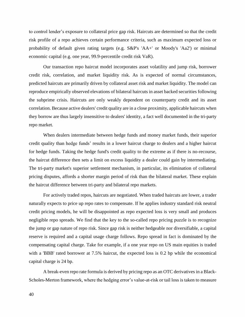
40
to control lender’s exposure to collateral price gap risk. Haircuts are determined so that the credit
risk profile of a repo achieves certain performance criteria, such as maximum expected loss or
probability of default given rating targets (e.g. S&P's 'AA+' or Moody's 'Aa2') or minimal
economic capital (e.g. one year, 99.9-percentile credit risk VaR).
Our transaction repo haircut model incorporates asset volatility and jump risk, borrower
credit risk, correlation, and market liquidity risk. As is expected of normal circumstances,
predicted haircuts are primarily driven by collateral asset risk and market liquidity. The model can
reproduce empirically observed elevations of bilateral haircuts in asset backed securities following
the subprime crisis. Haircuts are only weakly dependent on counterparty credit and its asset
correlation. Because active dealers' credit quality are in a close proximity, applicable haircuts when
they borrow are thus largely insensitive to dealers' identity, a fact well documented in the tri-party
repo market.
When dealers intermediate between hedge funds and money market funds, their superior
credit quality than hedge funds’ results in a lower haircut charge to dealers and a higher haircut
for hedge funds. Taking the hedge fund's credit quality to the extreme as if there is no-recourse,
the haircut difference then sets a limit on excess liquidity a dealer could gain by intermediating.
The tri-party market's superior settlement mechanism, in particular, its elimination of collateral
pricing disputes, affords a shorter margin period of risk than the bilateral market. These explain
the haircut difference between tri-party and bilateral repo markets.
For actively traded repos, haircuts are negotiated. When traded haircuts are lower, a trader
naturally expects to price up repo rates to compensate. If he applies industry standard risk neutral
credit pricing models, he will be disappointed as repo expected loss is very small and produces
negligible repo spreads. We find that the key to the so-called repo pricing puzzle is to recognize
the jump or gap nature of repo risk. Since gap risk is neither hedgeable nor diversifiable, a capital
reserve is required and a capital usage charge follows. Repo spread in fact is dominated by the
compensating capital charge. Take for example, if a one year repo on US main equities is traded
with a 'BBB' rated borrower at 7.5% haircut, the expected loss is 0.2 bp while the economical
capital charge is 24 bp.
A break-even repo rate formula is derived by pricing repo as an OTC derivatives in a Black-
Scholes-Merton framework, where the hedging error’s value-at-risk or tail loss is taken to measure
41
economic capital. It consists of a cost of fund component, a risk charge representing the expected
repo loss, and a capital charge at the shadow cost of capital. In particular, economic capital is
negatively linear in repo haircuts, so is the fair repo spread. Repo haircuts and repo spread as a
dual therefore work like a tandem.
From the borrower’s perspective, the all-in funding rate allows an optimal choice of
haircuts that balances, and settles uniquely between repo’s dual pricing measures. The tandem
allows a repo to be priced in a naturally counter-cyclical manner, a solution to address repo haircuts’
procyclicality and repo funding market instability induced thereafter. In a credit expansion cycle,
for example, traded repo haircuts tend to be low, but lower haircuts lead to higher economic capital
and higher capital charges in repo pricing, thus deterring an excessive build-up of leverage.
When a market stress is developing with heightened uncertainty, repo haircuts are expected
to rise. For borrowers wanting to maintain the same leverage (aka the same haircut), the model
requires a reduced repo tenor, to control the economic risk via EC, explaining the observed
tendency of lenders shortening repo tenors. The model could aid future econometric studies of
repo haircuts, repo pricing and their determinants, which will be strongly desired once relevant
transaction data is available.
References
Ashcraft, A., N. Gârleanu, and L. H. Pedersen, Two Monetary Tools: Interest Rates and Haircuts,
NBER Macroeconomics Annual (25), 2010.
Andersen , L., M. Pykhtin, and A. Sokol, Rethinking the Margin Period of Risk, Journal of Credit
Risk, Vol. 13, No. 1, 2017.
Auh, J. K. and M. Landoni (2016), Loan Terms and Collateral: Evidence from the Bilateral Repo
Market, ssrn preprint.
Baklanova, V., C. Caglio, M. Cipriani, and A. Copeland (2019), The Use of Collateral in Bilateral
Repurchase and Securities Lending Agreements, Review of Economic Dynamics,
33(2019), pp 228-249.
Bielecki, T. (2008), Rating SME transactions, Moody's Investor Services, May 2008.

42
BIS Committee on the Global Financial System (CGFS 2010), the role of margin requirements
and haircuts in procyclicality, BIS-CGFS Paper No.36 March 2010.
BIS -- the BASEL Committee on Banking Supervision (BCBS 2016), Minimum capital
requirements for market risk, Jan 2016.
BIS -- the BASEL Committee on Banking Supervision (BCBS 2020), Minimum Haircut Floors
for Securities Financing Transactions, CRE 56, effective Jan 2022.
Breach, T. and T. B. King, Securities Financing and Asset Markets: New Evidence, FRB working
paper, November 27, 2018
Brunnermerer, M. K. and L.H. Pederson (2009), Market Liquidity and Funding Liquidity, Review
of Financial Studies, 22(6) pp. 2201-2238.
Cai, N., S.G. Kou, and Z.J. Liu (2014), A Two-sided Laplace Inversion Algorithm with
Computable Error Bounds and Its Applications in Financing Engineering, Adv. Appl. Prob.,
46, pp 766-789.
Comotto, R. (2012), Haircuts and Initial Margins in the Repo Market, International Capital
Markets Association (ICMA), European Repo Council.
Copeland, A., A. Martin and M. Walker (2014), Repo Runs: Evidence from the Tri-Party Repo
Market, Journal of Finance, 69(6), pp 2343-2380.
Copeland, A., D. Duffie, A. Martin, and S. McLaughlin (2012). Key Mechanics of the U.S. Tri-
Party Repo Market. FRBNY Economic Policy Review.
Dang, T. V., G Gorton, and B. Holmstrom (2013). Haircuts and Repo Chains, http:
//www.columbia.edu/~td2332/Paper_Repo.pdf, Columbia University, Working paper.
Duffie, D., S. Das, N. Kapadia, and L. Saita (2007). Common Failings: How Corporate Defaults
Are Correlated. Journal of Finance, 72 (1), 93-117.
Duffie, D. (2011), Measuring Corporate Defaults, Oxford University Press.
Eraker, B. (2004). Do Stock Prices and Volatility Jump? Reconciling Evidence from Spot and
Option Prices, Journal of Finance, 59(3), pp 1368-1403.
Eraker, B., M. Johannes, and N. Polson (2003), The Impact of Jumps in Returns and Volatility,
Journal of Finance, 53, pp 1269-1300.
Financial Stability Board (FSB, 2015). Transforming shadow banking to resilient market-based
finance: regulatory framework for haircuts on non-centrally cleared securities financing
transactions.

43
Gorton, G. and A. Metrick (2012). Securitized Banking and the Run on Repo, Journal of Financial
Economics, 104 (3), pp 425-451.
Gorton, G., A. Metrick, and L. Xie (2014). The Flight from Maturity, NBER Working Paper No.
20027.
Green, A., C. Kenyon, and C. Dennis, 2014, KVA: capital valuation adjustment by replication,
Risk December, pp 82-87.
Hu, G. X., J. Pan, and J. Wang (2019). Tri-party Repo Pricing, NBER working paper No. 21502,
March 2019.
Infante, S. (2019). Liquidity Windfalls: The Consequences of Repo Rehypothecation, Journal of
Financial Economics, 132(1), pp 42-63.
Kou, S.G. (2002). A Jump-Diffusion Model for Option Pricing, Management Science, 48 (8), pp
1086-1101.
Krishnamurthy, A., S. Nagel, and D. Orlov (2014). Sizing up Repo, Journal of Finance, 69 (6), pp
2381–2417.
Lou, W. (2017). Haircutting Non-cash Collateral, Risk, September 2017, 84-89.
Lou, W. (2016). Gap Risk KVA and Repo Pricing, Risk, November 2016, 70-75.
Lou, W. (2019). The Fair Basis, Risk, May 2019, or https: //papers.ssrn.com/sol3/ papers.cfm?
abstract_id=3030498.
Martin, A., D. Skeie, and E.L. von Thadden (2014). Repo Runs, Review of Financial Studies,
27(4), 957-989.
Merton, R. (1976). Option Pricing when Underlying Stock Returns are Discontinuous. Journal of
Financial Economics, 3, 125-144.
Parlatore, C. (2019). Collateralizing liquidity. Journal of Financial Economics, 131, 299-322.
Prampolini, A. and M. Morini, 2018, Derivatives Hedging, Capital and Leverage, SSRN working
paper, https://papers.ssrn.com/sol3/papers.cfm?abstract_id=2699136, July.
Standard & Poor’s (S&P 2015), Default, Transition, and Recovery: 2015 Annual Global Corporate
Default Study and Rating Transitions.

44
Appendix A. Proof of Haircut Loss
The loss function defined in equation (1) is driven by a kernel function 𝐻(𝑡, 𝑢) =
(1−ℎ
1−𝑔−
𝐵𝑡+𝑢
𝐵𝑡)
+
, where g is a constant liquidity premium and h is a constant haircut. Let 𝑋(𝑡, 𝑢) =
𝐵𝑡+𝑢
𝐵𝑡. X(t,u)-1 is one period simple return of the security.
For an arbitrary h* satisfying h*>h, rewrite the indicator function as,
𝐼 [𝑋(𝑡, 𝑢) ≤1−ℎ
1−𝑔] = 𝐼 [𝑋(𝑡, 𝑢) ≤
1−ℎ∗
1−𝑔] + 𝐼 [
1−ℎ∗
1−𝑔< 𝑋(𝑡, 𝑢) ≤
1−ℎ
1−𝑔] (A.1)
And the loss kernel as follows,
𝐻(𝑡, 𝑢) = (1−ℎ
1−𝑔− 𝑋(𝑡, 𝑢)) 𝐼 [𝑋(𝑡, 𝑢) ≤
1−ℎ
1−𝑔] = (
1−ℎ∗
1−𝑔− 𝑋(𝑡, 𝑢))
+
+ℎ∗−ℎ
1−𝑔𝐼 [𝑋(𝑡, 𝑢) ≤
1−ℎ∗
1−𝑔] + (
1−ℎ
1−𝑔− 𝑋(𝑡, 𝑢)) 𝐼 [
1−ℎ∗
1−𝑔< 𝑋(𝑡, 𝑢) ≤
1−ℎ
1−𝑔] (A.2)
Let 𝑏 =ℎ∗−ℎ
1−𝑔, b>0 since h*>h, and 𝐻∗(𝑡, 𝑢) = (
1−ℎ∗
1−𝑔− 𝑋(𝑡, 𝑢))
+
, then we have,
𝐻(𝑡, 𝑢) = 𝐻∗(𝑡, 𝑢) + 𝑏𝐼 [𝑋(𝑡, 𝑢) ≤1−ℎ∗
1−𝑔] + (
1−ℎ
1−𝑔− 𝑋(𝑡, 𝑢)) 𝐼 [
1−ℎ∗
1−𝑔< 𝑋(𝑡, 𝑢) ≤
1−ℎ
1−𝑔] (A.3)
Now consider random variable 𝐼[𝐻(𝑡, 𝑢) > 𝑏] for a given pair of (h,b). Define ℎ∗ = ℎ +
𝑏(1 − 𝑔). Obviously,
𝐼[𝐻(𝑡, 𝑢) > 𝑏] = 𝐼 [𝑋(𝑡, 𝑢) ≤1−ℎ∗
1−𝑔] = 𝐼[𝐻∗(𝑡, 𝑢) > 0] (A.4)
Therefore, the kernel cumulative distribution satisfies,
Pr(𝐻(𝑡, 𝑢) > 𝑏) = 𝐸[𝐼[𝐻(𝑡, 𝑢) > 𝑏] ] = Pr (𝐻∗(𝑡, 𝑢) > 0) (A.5)
This could be made more general as follows,
Pr(𝐻(𝑡, 𝑢) > 𝑏) = Pr (𝐻∗(𝑡, 𝑢) > 𝑏∗) (A.6)
where ℎ∗ + 𝑏∗(1 − 𝑔) = ℎ + 𝑏(1 − 𝑔), 𝑏 ≥ 0 and 𝑏∗ ≥ 0.
Because the loss function L is a simple function of the kernel, if F(x|h) denotes the
cumulative loss distribution with haircut h, then F(b*|h*)= F(b|h).

45
Next consider the expectation of the truncated loss, E[L(t,u)| L(t,u)>l]. Noting (A.4),
𝐻(𝑡, 𝑢) ∗ 𝐼[𝐻(𝑡, 𝑢) > 𝑏] = 𝐻(𝑡, 𝑢) ∗ 𝐼[𝐻∗(𝑡, 𝑢) > 0] = 𝐻∗(𝑡, 𝑢) + 𝑏𝐼[𝐻∗(𝑡, 𝑢) > 0]
𝐸[𝐻(𝑡, 𝑢)|𝐻(𝑡, 𝑢) > 𝑏] =𝐸[𝐻(𝑡,𝑢)∗𝐼[𝐻(𝑡,𝑢)>𝑏]]
Pr(𝐻(𝑡,𝑢)>𝑏)=
𝐸[𝐻∗(𝑡,𝑢)]
Pr(𝐻∗(𝑡,𝑢)>0)+ 𝑏 (A.7)
Applying the constant to get the expected truncated loss,
𝐸[𝐿(𝑡, 𝑢)|𝐿(𝑡, 𝑢) > 𝑙] =𝐸[𝐿∗(𝑡,𝑢)]
Pr(𝐿∗(𝑡,𝑢)>0)+ 𝑙, (A.8)
𝑙 = (1 − 𝑅𝑐)(1 − 𝑔)𝑀0𝑏
In the above, we have not considered counterparty default during the repo tenor of T.
Counterparty default as a single trigger event could happen at a small time interval prior to T, but
the magnitude of loss is still determined by the margin period immediately following the default.
The resultant loss distribution will need to integrate over the length of T but the integration does
not change the equality established in A.6 and A.8.