Regularized Adaptation of Fuzzy Inference Systems.Modelling the Opinion of a Medical Expert aboutPhysical Fitness: An Application
MOHIT KUMAR [email protected]
Institute of Occupational and Social Medicine, Faculty of Medicine, University of Rostock, D-18055 Rostock,
Germany
REGINA STOLL [email protected]
Institute of Occupational and Social Medicine, Faculty of Medicine, University of Rostock, D-18055 Rostock,
Germany
NORBERT STOLL [email protected]
Institute of Automation, Department of Electrical Engineering and Information Technology, University of
Rostock, D-18119 Rostock-Warnemnde, Germany
Abstract. This study presents a new approach to adaptation of Sugeno type fuzzy inference systems using
regularization, since regularization improves the robustness of standard parameter estimation algorithms leading to
stable fuzzy approximation. The proposed method can be used for modelling, identification and control of physical
processes. A recursive method for on-line identification of fuzzy parameters employing Tikhonov regularization is
suggested. The power of approach was shown by applying it to the modelling, identification, and adaptive control
problems of dynamic processes. The proposed approach was used for modelling of human-decisions (experience)
with a fuzzy inference system and for the fuzzy approximation of physical fitness with real world medical data.
Keywords: fuzzy approximation, model identification, ill-posed, regularization, nonlinear least squares, inverse
control, generalized predictive control
1. Introduction
Fuzzy systems have been widely applied for modelling complex processes and decision
problems (Zadeh (1973)). The main advantage of fuzzy inference system over classical
learning systems and neural networks is its linguistic interpretability of its function.
Automatic construction or tuning of the fuzzy systems from example data has been widely
explored for Sugeno type fuzzy inference system by Babuska (2000), Bodenhofer and
Bauer (2000), Espinosa and Vandewalle (2000), and Setnes et al (1998). The Sugeno type
fuzzy systems are supposed to ideally combine simplicity with good analytical properties
(Takagi and Sugeno (1985)). The general problem of estimating the parameters describing
Sugeno fuzzy system from data is ill-posed (Burger et al (2002)). Therefore, nonlinear
regularization theory has been employed and a numerical method based on generalized
Gauss-Newton was suggested for solving nonlinear regularized optimization problem by
Burger et al (2002). In this study, a recursive method for online learning of fuzzy system
employing Tikhonov regularization is suggested. This method is based on recursive
solution of a nonlinear least squares problem. The antecedent parameters are estimated by
Fuzzy Optimization and Decision Making, 2, 317–336, 2003# 2003 Kluwer Academic Publishers. Printed in The Netherlands.
solving a local approximation problem using generalized Gauss-Newton method. These
local mappings facilitate the minimal disturbance principle (Widrow and Lehr (1990)),
which is particularly important in on-line learning. The proposed numerical method was
applied for fuzzy identification, prediction, and adaptive control of a time-varying plant
based on generalized predictive control (GPC) and inverse model strategies.
The second part of paper deals with the regularized adaptation of fuzzy expert systems
applied to a medicine problem. Such an expert system uses knowledge to solve problems
that would, under normal circumstances, require a medical expert. In medicine, expert
systems are required to interpret medical data and then to provide diagnostic and
therapeutic advice, suggesting the prognosis of disease, guiding patient management,
and monitoring patient medical data. Based on the developed algorithm, an attempt to
approximate the physical fitness with an interpretable fuzzy expert system is made and
shown to provide good results. The training data consists of real world physiological
parameter measurements and the fuzzy system was tuned by the uncertain advice of a
medical expert.
2. Problem Formulation
Let us consider a Sugeno fuzzy inference system (Fs: X ! Y ), mapping n-dimensional
input space (X ¼ X1 � X2 � : : : � Xn) to one dimensional real line with K different rules.
The ith rule is in the form:
If x1 is Ai1 and x2 is Ai2 . . . . and xn is Ain then y ¼ �i, for all i ¼ 1, 2, . . . , K. Assume
that Ai1, Ai2, . . . , Ain are non-empty fuzzy subsets of (X ¼ X1 � X2 � : : : � Xn)
respectively with membership functions �Aij: Xj ! [0, 1],
PKi¼1
Qnj¼1 �Aij
(xj) > 0 for all
x � X. The values �1, �2, . . . , �K are real numbers. So we have
Fsðx1; x2; . . . ; xnÞ ¼PK
i¼1 �i
Qnj¼1 �Aij
ðxjÞPKi¼1
Qnj¼1 �Aij
ðxjÞ; ð1Þ
where xj � [aj, bj] for all j ¼ 1, . . . , n.
For the mathematical description of fuzzy sets, we choose trapezoidal membership
functions which can be described by a finite set of parameters. The shape of membership
functions depends on a finite dimensional knot sequence t, partitioning the universe of
each input variable (xi � [ai, bi]) in to Pi linguistic terms. Let t ¼ ðt11; . . . ; t2P1�21 ; t12 ; . . . ;
t2P2�22 ; . . . ; t1n ; . . . ; t
2Pn�2n Þ � R1�L , such that for ith input, ai � t1i � : . . . : � t2Pi�2
i � biholds for all i ¼ 1, . . . , n. So Pi membership functions for ith input (A1i, A2i, . . . , APii
) can
be defined as:
A1iðxi; tÞ ¼1 if xi � ½ai; t1i �
�xiþt2it2i�t1
i
if xi � ½t1i ;t2i �0 otherwise
8><>:
KUMAR, STOLL AND STOLL318
Ajiðxi; tÞ ¼
xi�t2 j�3i
t2 j�2i
�t2 j�3i
if xi � ½t2j�3i ; t2j�2
i �1 if xi � ½t2j�2
i ; t2j�1i �
�xiþt2 ji
t2 ji�t
2 j�1i
if xi � ½t2j�1i ; t2ji �
0 otherwise
8>>>>><>>>>>:
APiiðxi; tÞ ¼xi�t
2Pi�3
i
t2Pi�2
i�t
2Pi�3
i
if xi � ½t2Pi�3i ; t2Pi�2
i �
1 if xi � ½t2Pi�2i ; bi�
0 otherwise
8><>:The total number of possible rules depends on the number of membership functions for
each input. If Pi is the number of membership functions defined over ith input then total
number of rules K ¼Qn
i¼1 Pi . The above choice of membership functions allowsPK
i¼1Qnj¼1 �Aij
ðxjÞ ¼ 1, simplifying the equation (1) as function of t.
Fsðx1; x2; . . . ; xnÞ ¼XKi¼1
�iBiðx1; x2; . . . ; xn; tÞ;
where
Biðx1; x2; . . . ; xn; tÞ ¼Qn
j¼1 �AijðxjÞPK
i¼1
Qnj¼1 �Aij
ðxjÞ:
Let x ¼ [x1, x2, . . . , xn], then
FsðxÞ ¼XKj¼1
�jBjðx; tÞ:
Let {(xk, yk )}k¼1,2, . . . ,m be a training data set, where xk ¼ (xk1, . . . , xkn) is k
th measured input
vector and yk is the corresponding measured output value. For the estimation of
consequent parameters (�1, �2, . . . , �K) and antecedent parameters (t) of the Sugeno
fuzzy system from training data, least squares criteria can be used. So, we want to
minimize the following functional:
�ð�1; �2; . . . ; �K ; tÞ ¼Xmi¼1
ðyi �XKj¼1
�jBjðxi; tÞÞ2:
Let us introduce following notations:
Y ¼ [ yi]i¼1,2, . . . ,m, � ¼ [�j] j¼1,2, . . . ,K, B(t) = [Bj(xi; t)]i¼1,2, . . . ,m; j¼1,2, . . . ,K.
So
�ð�; tÞ ¼ jjY � BðtÞ�jj2;
REGULARIZED ADAPTATION OF FUZZY INFERENCE SYSTEMS 319
where ||.|| denotes the usual Euclidean norm. The problem of finding a minimum to above
functional is ill-posed in the sense that arbitrarily small errors in the training data possibly
lead to arbitrarily large errors in the solution of minimization problem (Burger et al
(2002)), which necessitates the use of regularization methods. Applying Tikhonov
regularization, the functional to be minimized becomes
�ð�; tÞ ¼ jjY � BðtÞ�jj2 þ �1
XKj¼1
�2j þ �2jjt� t0jj2; ð2Þ
where t0 represents the initial guess about shape of membership functions and (�1, �2) are
the regularization parameters, which control the influence of the regularization terms. The
use of regularization replaces an ill-posed problem by a family of similar well-posed
problems through the introduction of regularization terms and regularization parameters. It
was shown by Binder et al (1994), Engl et al (1996), and Engl et al (1989) that minimizer
of equation (2) exists if �1 > 0 and �2 > 0. We can write equation (2) as
�ð�; tÞ ¼ jjY � BðtÞ�jj2 þ �1jj�jj2 þ �2jjt� t0jj2:
Above equation can be rewritten in the form
�ð�; tÞ ¼ jjZðtÞ �GðtÞ�jj2:
To preserve the linguistic interpretability of fuzzy system during learning, the membership
functions must be prevented from overlapping by imposing constraints on the positions of
knots i.e. for all i ¼ 1, . . , n
t1i � ai � �itjþ1i � t
ji � �i for all j ¼ 1; 2; ::; ð2Pi � 3Þ
bi � t2Pi�2i � �i
These constraints can be formulated in term of a matrix inequality Ct � h, similar to the
constrained problem formulated by Burger et al (2002). Finally the constrained regularized
optimization problem is
½�*; t*� ¼ arg minð�;tÞ½�ð�; tÞ ; Ct � h�:
3. Recursive Solution of Regularized Optimization Problem
The objective functional to be minimized is linear in � and non-linear in t. A method
based on generalized Gauss-Newton was suggested to solve the above optimization
problem by Burger et al (2002). However, application of fuzzy parameters adaptation to
on-line identification and adaptive control necessitates the recursive solution of the
KUMAR, STOLL AND STOLL320

optimization problem. This section suggests an algorithm to minimize above functional to
find optimal � and t from recursive data. The linear parameter (�) is adapted or identified
using well known recursive least squares estimation (LSE) and non-linear parameter (t) is
adapted by solving a nonlinear constrained local optimization problem using generalized
Gauss-Newton method. Let (�k*; tk*) denote the optimal fuzzy parameters estimated using k
data pairs and are defined as solution of the following two optimization problems:
tk* ¼ arg mint½ðyk � Bðxk ; tÞ�k�1* Þ2 þ �2ðkÞjjt� t*k�1jj2;Ct � h�;
where B(xk, t) ¼ [Bj(xk; t)]j=1,2, . . . ,K � R1�K and
�*k ¼ arg min�½�ð�; t*kÞ�:
The above optimization problem reduces to
�*k ¼ arg min�Xki¼1
ðyi � Bðxi; t*i Þ�Þ2 þ �1ðkÞjj�jj2" #
:
3.1. Algorithm
1. Let t0 denotes the initial guess about parameter t. Let �0 ¼ [0]K�1 and P0 ¼ �I(K�K),
where � is a large number.
2. k ¼ 1, choose �1 and �2(k).3. Let Z(t) ¼ [ yk (0)1xK]
T � R(Kþ1)�1 and
G(t) ¼ [B(xk, t) ; (�1)1/2(I )K�K] � R(Kþ1)�K.
4. Solve min [||Zðtk�1* Þ � Gðtk�1* Þ||2] for optimal value �k*with fixed tk�1* by recursive LSE
algorithm as
P jþ1 ¼ Pj � Pj½Grð jÞ�TGrð jÞP j
1þ Grð jÞPj½Grð jÞ�T;
� jþ1 ¼ � j þ Pjþ1½Grð jÞ�T ½Zrð jÞ � Grð jÞ� j�;
for j¼ 1, 2, . . . , (Kþ 1) with �1¼ �k�1, P1¼ Pk�1. The vectorsGr( j ) and Zr( j ) denotes
the jth row ofmatrixG(tk�1* ) and Z(tk�1* ) respectively. Finally�k*¼ �Kþ2 and Pk ¼ PKþ2.
5. Let Z1(t) ¼yk
ð�2ðkÞÞ1=2ðt� tk�1* Þ
24 35 � Rð1þLÞ�1;W1ðtÞ ¼Bðxk; tÞ
ð0ÞL�K
24 35:6. Let residual: r (t) ¼ Z1(t) � W1(t)�k* and J ¼ rV(t) be the derivative of r (t) with respect
to t, computed by the method of finite differences. J is a full rank matrix as a result of
using regularization.
7. Solve mins [||r(tk�1* ) þ Js||2 ; Cs � h�Ctk�1* ] based on algorithm given by Lawson and
Hanson (1995).
8. tk*¼ tk�1* þ s.
9. Repeat
REGULARIZED ADAPTATION OF FUZZY INFERENCE SYSTEMS 321
a) k :¼ k þ 1 and choose �2(k).b) Update �k
* with new data pair and from �k�1* , Pk�1 as follows:
Pk ¼ Pk�1 �Pk�1½Bðxk ; t*k�1Þ�TBðxk ; t*k�1ÞPk�1
1þ Bðxk ; t*k�1ÞPk�1½Bðxk ; t*k�1Þ�T
�*k ¼ �*k�1 þ Pk ½Bðxk ; t*k�1Þ�T ½yk � Bðxk ; t*k�1Þ�*k�1�
c) Update tk* as in steps from 5th to 8th with new data pair.
till the last data pair.
This algorithm can be applied for the fuzzy modelling of dynamic processes from the
noisy data. The off-line version of this algorithm together with the line search method was
applied to some typical fuzzy modelling examples with uncertain data by Burger et al
(2000). The proposed algorithm extends the use of regularized fuzzy adaptation for on-line
identification, prediction and adaptive control.
4. Application to Identification, Prediction and Control
4.1. On-Line Identification
The above suggested algorithm can be applied for on-line identification with the choice of
regularization parameters �2(k) as follows
�2ðkÞ ¼ �k > 0:
where � is a constant. For the comparison of algorithm performance with the existing
techniques, an example from Jang et al (1997) is considered. The unknown function to be
identified by fuzzy inference system has the form
f ðuÞ ¼ 0:6 sinð�uÞ þ 0:3 sinð3�uÞ þ 0:1 sinð5�uÞ:
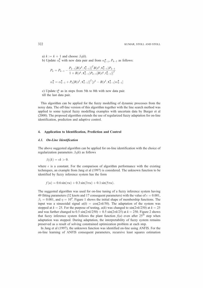
The suggested algorithm was used for on-line tuning of a fuzzy inference system having
49 fitting parameters (32 knots and 17 consequent parameters) with the value of � ¼ 0.001,
�1 ¼ 0.001, and � ¼ 104. Figure 1 shows the initial shape of membership functions. The
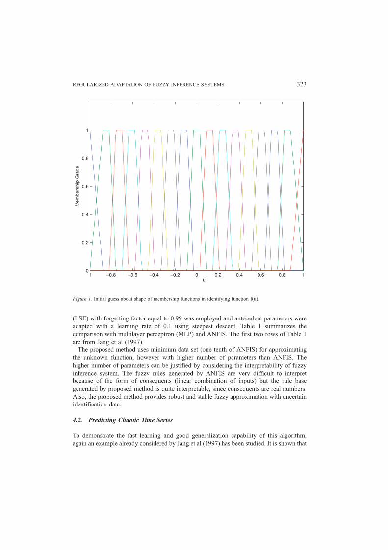
input was a sinusoidal signal u(k) ¼ cos(2pk/50). The adaptation of the system was
stopped at k ¼ 25. For the purpose of testing, u(k) was changed to sin(2pk/250) at k ¼ 25
and was further changed to 0.5 sin(2pk/250) þ 0.5 sin(2pk/25) at k ¼ 250. Figure 2 shows
that fuzzy inference system follows the plant function f (u) even after 25th step when
adaptation was stopped. During adaptation, the interpretability of fuzzy system remains
preserved as a result of solving constrained optimization problem at each step.
In Jang et al (1997), the unknown function was identified on-line using ANFIS. For the
on-line learning of ANFIS consequent parameters, recursive least squares estimation
KUMAR, STOLL AND STOLL322
(LSE) with forgetting factor equal to 0.99 was employed and antecedent parameters were
adapted with a learning rate of 0.1 using steepest descent. Table 1 summarizes the
comparison with multilayer perceptron (MLP) and ANFIS. The first two rows of Table 1
are from Jang et al (1997).
The proposed method uses minimum data set (one tenth of ANFIS) for approximating
the unknown function, however with higher number of parameters than ANFIS. The
higher number of parameters can be justified by considering the interpretability of fuzzy
inference system. The fuzzy rules generated by ANFIS are very difficult to interpret
because of the form of consequents (linear combination of inputs) but the rule base
generated by proposed method is quite interpretable, since consequents are real numbers.
Also, the proposed method provides robust and stable fuzzy approximation with uncertain
identification data.
4.2. Predicting Chaotic Time Series
To demonstrate the fast learning and good generalization capability of this algorithm,
again an example already considered by Jang et al (1997) has been studied. It is shown that
Figure 1. Initial guess about shape of membership functions in identifying function f(u).
REGULARIZED ADAPTATION OF FUZZY INFERENCE SYSTEMS 323
trained fuzzy inference system can be used to predict the future values of a chaotic time
series. The performance obtained in this example is compared with other methods. The
time series is generated by simulating the chaotic Mackey-Glass differential delay equation
i.e.
dx
dt¼ 0:2xðt � 17Þ
1þ x10ðt � 17Þ � 0:1xðtÞ;
with xð0Þ ¼ 1:2; xðtÞ ¼ 0 ; for t < 0:
The aim of the problem is to predict the value of x(t þ 6) by using a set of past values i.e.
[x(t � 18), x(t � 12), x(t � 6), x(t)]. Fourth-order Runge-Kutta method was used for the
simulation of above equation and 250 data pairs were extracted for the training set of fuzzy
inference system. Checking data set for validating the identified fuzzy system consists of
500 data pairs which is same as in Jang et al (1997), hence allowing the direct comparison
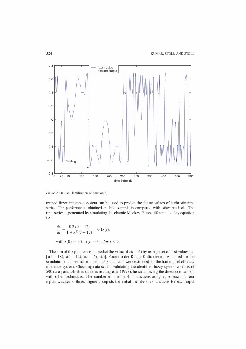
with other techniques. The number of membership functions assigned to each of four
inputs was set to three. Figure 3 depicts the initial membership functions for each input
Figure 2. On-line identification of function f(u).
KUMAR, STOLL AND STOLL324
variable. Such a fuzzy system was tuned on-line till 250 steps having 97 fitting
parameters (16 knots and 81 consequent parameters) with � ¼ 0.5, �1 ¼ 0.001, � ¼104, and afterwards it was used to predict 500 points of checking data set. To measure the
prediction error non-dimensional error index (NDEI) is defined as the root mean square
divided by the standard deviation of the target series. Figure 4 shows the generalization
capability of regularized fuzzy system learned on-line. Results shown in Table 2 (last four
rows are from Jang et al. (1997)) indicate that regularized learning of fuzzy systems
requires minimum training data for the fuzzy approximation. We find that the prediction
error of ANFIS is smaller than the error of regularized adaptation method. However,
Table 1. Comparison with other identifiers.
Method Parameters number
Time steps
of Adaptation
Backpropagation MLP 261 50000
ANFIS 35 250
Regularized Fuzzy Adaptation 49 25
Figure 3. Initial guess about shape of membership functions for all four inputs in predicting time series.
REGULARIZED ADAPTATION OF FUZZY INFERENCE SYSTEMS 325
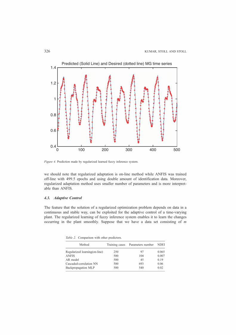
we should note that regularized adaptation is on-line method while ANFIS was trained
off-line with 499.5 epochs and using double amount of identification data. Moreover,
regularized adaptation method uses smaller number of parameters and is more interpret-
able than ANFIS.
4.3. Adaptive Control
The feature that the solution of a regularized optimization problem depends on data in a
continuous and stable way, can be exploited for the adaptive control of a time-varying
plant. The regularized learning of fuzzy inference system enables it to learn the changes
occurring in the plant smoothly. Suppose that we have a data set consisting of m
Table 2. Comparison with other predictors.
Method Training cases Parameters number NDEI
Regularized learning(on-line) 250 97 0.065
ANFIS 500 104 0.007
AR model 500 45 0.19
Cascaded-correlation NN 500 693 0.06
Backpropagation MLP 500 540 0.02
Figure 4. Prediction made by regularized learned fuzzy inference system.
KUMAR, STOLL AND STOLL326
observations [(xi, yi)]i¼1,2, . . . ,m which serves as training data for the learning of fuzzy
system. The problem consist of minimizing the functional
½�*; t*� ¼ arg minXmi¼1
ðyi � �Kj¼1�jBjðxi; tÞÞ2 þ �1jj�jj2 þ �2jjt� t0jj2
" #: ð3Þ
Assume that the function Bj satisfy the Lipschitz-estimate
jBjðu; tÞ � Bjðbu; tÞj < �Lju� buj;for all u, ub and t with some nonnegative real constant L. Let (�k, t k ) be the solution of
minimization problem (3) with training data [Xk, Yk], resulting the fuzzy approximation
of desired function (model of plant or controller) at any time. Any model based stable
control strategy can be used to control the plant at this time. Now, suppose that the
dynamics of plant changes and we collect a new data set [X, Y ], consisting of m
observations. Again, we solve the minimization problem (3) with new training data set
[X, Y ]. The stability and convergence analysis of this problem states following results
from Burger et al (2000).
Preposition (Stability) 1. Let �1 > 0, Yk ! Y and Xk ! X. Then the according sequence
of minimizers (�k, t k ) of (3) has a convergent subsequence and the limit of every
convergent subsequence is a minimizer of (3).
The proof of above preposition follows from Burger et al (2000). Let us assume that the
new training data set and old data set satisfy following equations
jjX k � X jj < � k and jjYk � Y jj < � k : ð4Þ
THEOREM (CONVERGENCE) 1. Assume that minimizer of problem (3) exists. Moreover,
let (�k, �k) be a sequence converging to (0, 0) and denote by (�k, t k) the according
sequence of minimizers of (3) with data [Xk, Yk], satisfying (4). Then (�k, t k) has a
convergent subsequence and the limit of every convergent subsequence is a minimizer of
(3) with data [X, Y] if the regularization parameters satisfy
�k1 ! 0; �k
2 ! 0;maxð�k ; �kÞ
�k1
! 0;
9� > 0 : ð�k1=�
k2Þ > �:
Again the proof of above theorem follows from Burger et al (2000). So we note that by
solving a regularized minimization problem, it is possible to get a stable approximation of
an unknown function. Thus the recursive solution of minimization problem (3) allows us
to approximate any time-varying function in a natural stable way, since the solution of
minimization problem depends upon data samples in a continuous and stable manner.
REGULARIZED ADAPTATION OF FUZZY INFERENCE SYSTEMS 327
The proposed algorithm can be applied as such with a suitable choice of regularization
parameters �1 ¼ �2(k) ¼ � > 0. The regularization parameter �2 is chosen independent of
time, contrary to on-line identification, where regularization parameter increases linearly
with time. The optimal value of regularization parameter is always a compromise between
stability and accuracy. A higher value of regularization parameter provides more damping
to oscillations but may results in larger error. To demonstrate the feasibility of our
approach, we consider a time-varying plant described by following discrete dynamical
equation
yðk þ 1Þ ¼ yðkÞuðkÞ1þ rðkÞy2ðkÞ � tan uðkÞ; ð5Þ
where y(k) and u(k) are the state and control action respectively at time step k and r (k) is a
parameter of plant that changes with time and the variation of this parameter with time is
not known. Among the various choices of control strategies, we consider only Inverse
Control and Generalized Predictive Control.
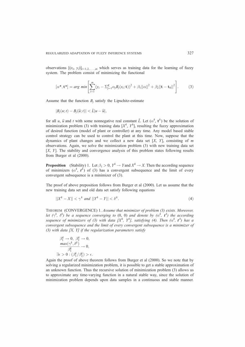
4.3.1. Inverse Control
The idea behind inverse control is to capture the inverse dynamics of plant using a fuzzy
inference system. The fuzzy model is trained to map the inverse of the function describing
the dynamics of plant to be controlled. The trained fuzzy system is then used to generate
control actions for the given desired output. The learning of a fuzzy system can continue
with time, enabling it to be used in adaptive context, when the plant is time varying. Let us
consider the plant described by equation (5) and goal is to track the reference trajectory
given by equation
yrðk þ 1Þ ¼ 0:6sinðk=11Þ þ 0:2sinðk=3Þ:
Let r(k) varies with time in following manner:
rðkÞ ¼
1 when 0 < k � 50;2 when 50 < k � 100;3 when 100 < k � 150;4 when 150 < k � 200:
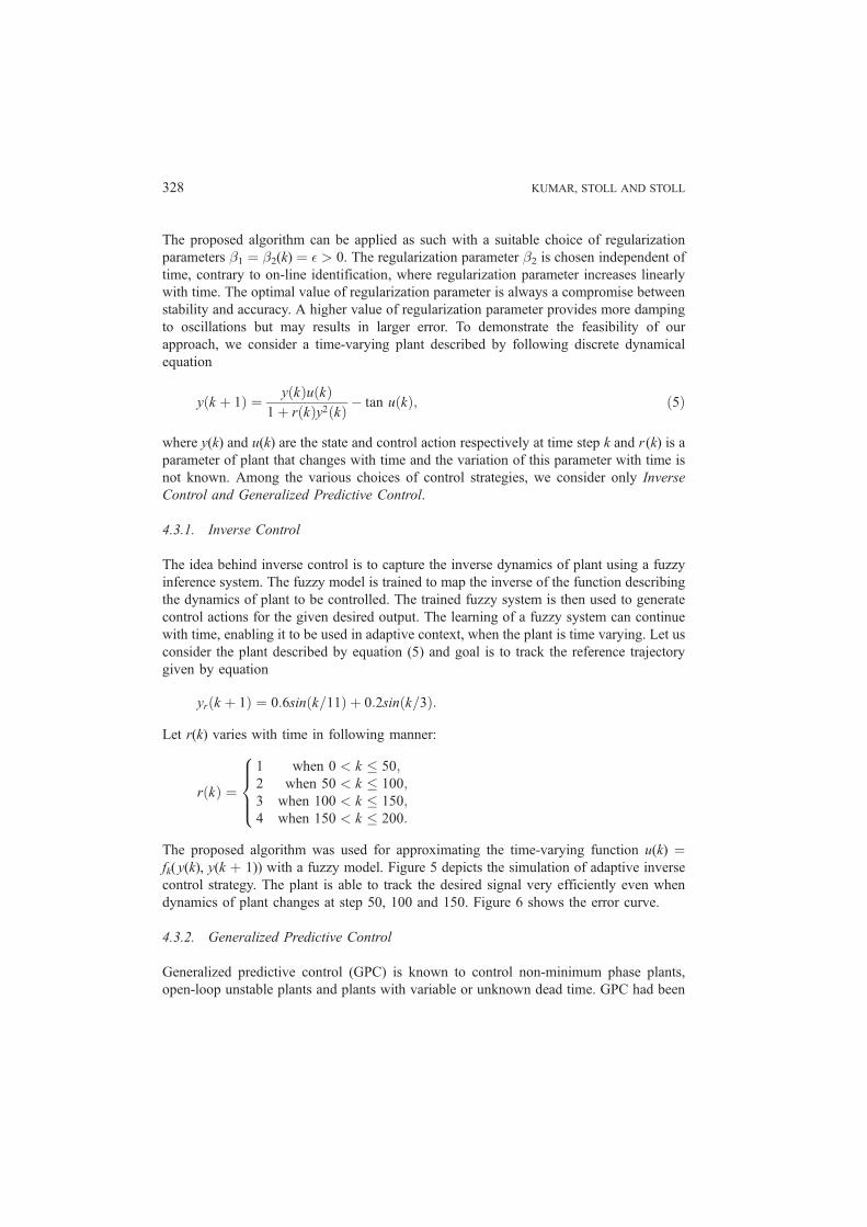
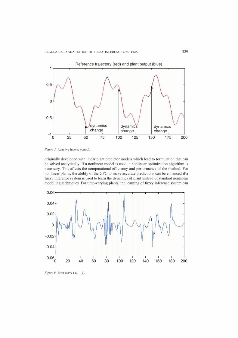
8>><>>:The proposed algorithm was used for approximating the time-varying function u(k) ¼fk( y(k), y(k þ 1)) with a fuzzy model. Figure 5 depicts the simulation of adaptive inverse
control strategy. The plant is able to track the desired signal very efficiently even when
dynamics of plant changes at step 50, 100 and 150. Figure 6 shows the error curve.
4.3.2. Generalized Predictive Control
Generalized predictive control (GPC) is known to control non-minimum phase plants,
open-loop unstable plants and plants with variable or unknown dead time. GPC had been
KUMAR, STOLL AND STOLL328
originally developed with linear plant predictor models which lead to formulation that can
be solved analytically. If a nonlinear model is used, a nonlinear optimization algorithm is
necessary. This affects the computational efficiency and performance of the method. For
nonlinear plants, the ability of the GPC to make accurate predictions can be enhanced if a
fuzzy inference system is used to learn the dynamics of plant instead of standard nonlinear
modelling techniques. For time-varying plants, the learning of fuzzy inference system can
Figure 5. Adaptive inverse control.
Figure 6. Error curve ( yr � y).
REGULARIZED ADAPTATION OF FUZZY INFERENCE SYSTEMS 329
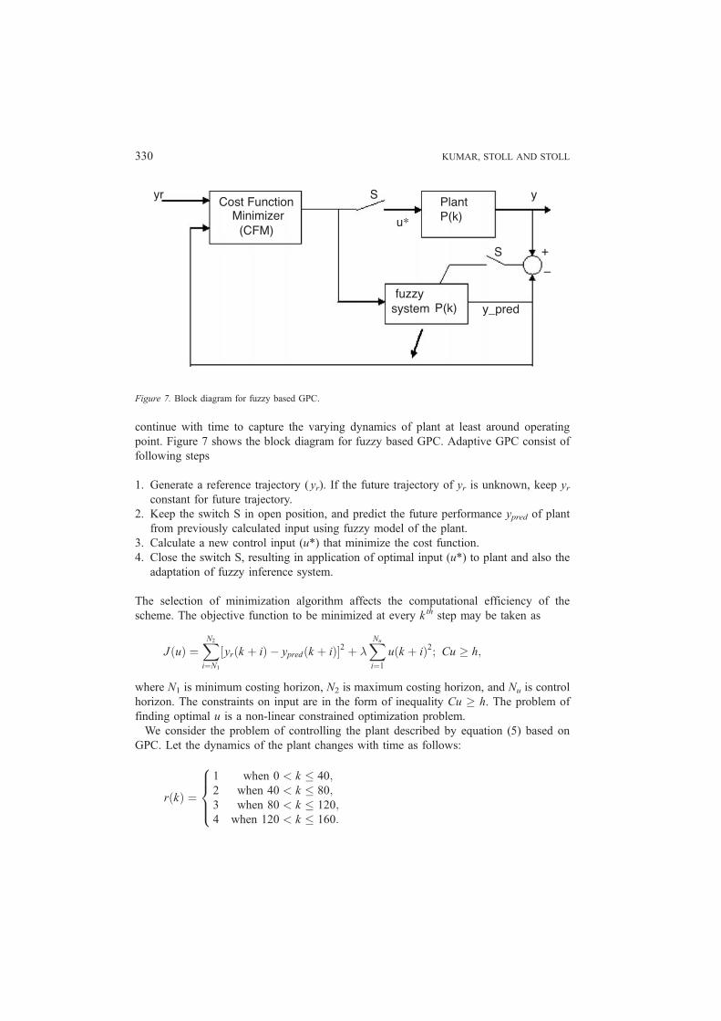
continue with time to capture the varying dynamics of plant at least around operating
point. Figure 7 shows the block diagram for fuzzy based GPC. Adaptive GPC consist of
following steps
1. Generate a reference trajectory ( yr). If the future trajectory of yr is unknown, keep yrconstant for future trajectory.
2. Keep the switch S in open position, and predict the future performance ypred of plant
from previously calculated input using fuzzy model of the plant.
3. Calculate a new control input (u*) that minimize the cost function.
4. Close the switch S, resulting in application of optimal input (u*) to plant and also the
adaptation of fuzzy inference system.
The selection of minimization algorithm affects the computational efficiency of the
scheme. The objective function to be minimized at every k th step may be taken as
JðuÞ ¼XN2
i¼N1
½yrðk þ iÞ � ypredðk þ iÞ�2 þ XNu
i¼1
uðk þ iÞ2; Cu � h;
where N1 is minimum costing horizon, N2 is maximum costing horizon, and Nu is control
horizon. The constraints on input are in the form of inequality Cu � h. The problem of
finding optimal u is a non-linear constrained optimization problem.
We consider the problem of controlling the plant described by equation (5) based on
GPC. Let the dynamics of the plant changes with time as follows:
rðkÞ ¼
1 when 0 < k � 40;2 when 40 < k � 80;3 when 80 < k � 120;4 when 120 < k � 160:
8>><>>:
Figure 7. Block diagram for fuzzy based GPC.
KUMAR, STOLL AND STOLL330
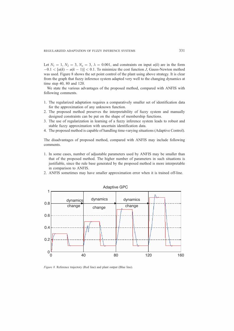
Let N1 ¼ 1, N2 ¼ 3, Nu ¼ 3, ¼ 0.001, and constraints on input u(k) are in the form
�0.1 < [u(k) � u(k � 1)] < 0.1. To minimize the cost function J, Gauss-Newton method
was used. Figure 8 shows the set point control of the plant using above strategy. It is clear
from the graph that fuzzy inference system adapted very well to the changing dynamics at
time step 40, 80 and 120.
We state the various advantages of the proposed method, compared with ANFIS with
following comments.
1. The regularized adaptation requires a comparatively smaller set of identification data
for the approximation of any unknown function.
2. The proposed method preserves the interpretability of fuzzy system and manually
designed constraints can be put on the shape of membership functions.
3. The use of regularization in learning of a fuzzy inference system leads to robust and
stable fuzzy approximation with uncertain identification data.
4. The proposed method is capable of handling time-varying situations (Adaptive Control).
The disadvantages of proposed method, compared with ANFIS may include following
comments.
1. In some cases, number of adjustable parameters used by ANFIS may be smaller than
that of the proposed method. The higher number of parameters in such situations is
justifiable, since the rule base generated by the proposed method is more interpretable
in comparison to ANFIS.
2. ANFIS sometimes may have smaller approximation error when it is trained off-line.
Figure 8. Reference trajectory (Red line) and plant output (Blue line).
REGULARIZED ADAPTATION OF FUZZY INFERENCE SYSTEMS 331
5. Fuzzy Approximation to Physical Fitness
We consider the classical problem of physical fitness estimation based on the
interpretation of various physiological parameters measurements. We approximate the
functional relationship between physical fitness and the measured physiological
parameters with an interpretable fuzzy system to interpret medical data and then to
provide diagnostic and therapeutic advice. It is clear that this functional relationship is
not so easy to define even in linguistic terms due to inherent presence of vagueness,
linguistic uncertainty, hesitation, measurement imprecision, natural diversity and sub-
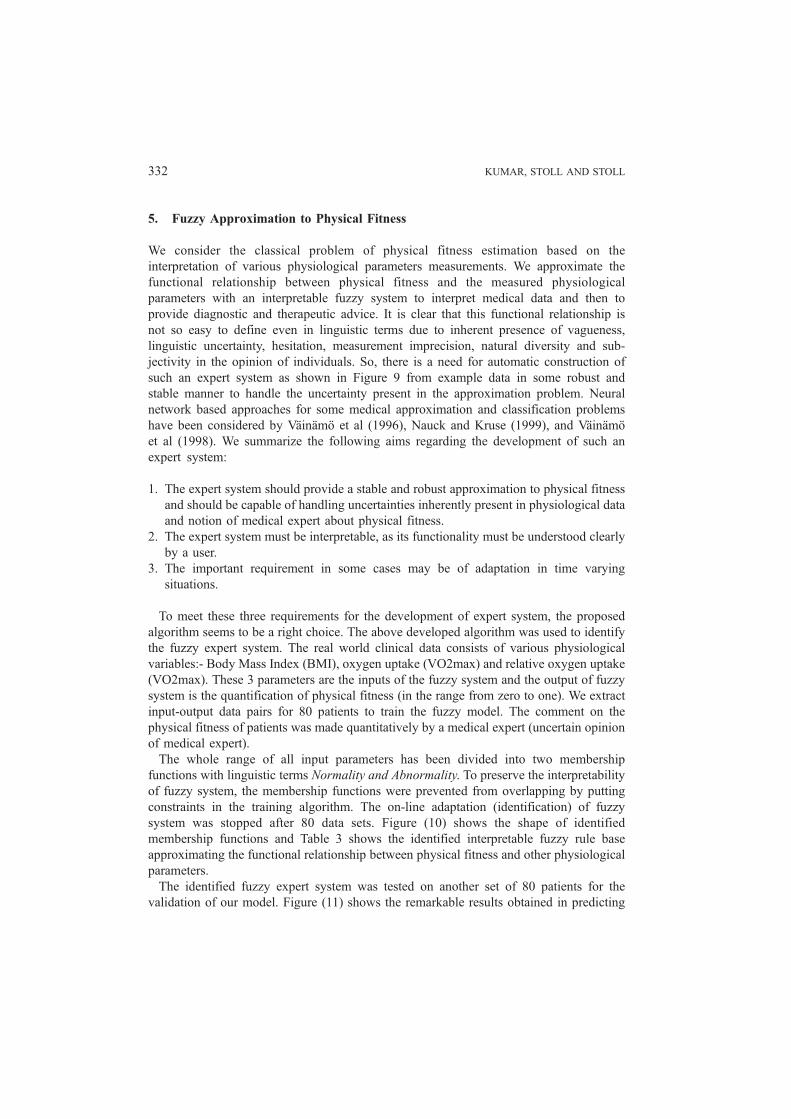
jectivity in the opinion of individuals. So, there is a need for automatic construction of
such an expert system as shown in Figure 9 from example data in some robust and
stable manner to handle the uncertainty present in the approximation problem. Neural
network based approaches for some medical approximation and classification problems
have been considered by Vainamo et al (1996), Nauck and Kruse (1999), and Vainamo
et al (1998). We summarize the following aims regarding the development of such an
expert system:
1. The expert system should provide a stable and robust approximation to physical fitness
and should be capable of handling uncertainties inherently present in physiological data
and notion of medical expert about physical fitness.
2. The expert system must be interpretable, as its functionality must be understood clearly
by a user.
3. The important requirement in some cases may be of adaptation in time varying
situations.
To meet these three requirements for the development of expert system, the proposed
algorithm seems to be a right choice. The above developed algorithm was used to identify
the fuzzy expert system. The real world clinical data consists of various physiological
variables:- Body Mass Index (BMI), oxygen uptake (VO2max) and relative oxygen uptake
(VO2max). These 3 parameters are the inputs of the fuzzy system and the output of fuzzy
system is the quantification of physical fitness (in the range from zero to one). We extract
input-output data pairs for 80 patients to train the fuzzy model. The comment on the
physical fitness of patients was made quantitatively by a medical expert (uncertain opinion
of medical expert).
The whole range of all input parameters has been divided into two membership
functions with linguistic terms Normality and Abnormality. To preserve the interpretability
of fuzzy system, the membership functions were prevented from overlapping by putting
constraints in the training algorithm. The on-line adaptation (identification) of fuzzy
system was stopped after 80 data sets. Figure (10) shows the shape of identified
membership functions and Table 3 shows the identified interpretable fuzzy rule base
approximating the functional relationship between physical fitness and other physiological
parameters.
The identified fuzzy expert system was tested on another set of 80 patients for the
validation of our model. Figure (11) shows the remarkable results obtained in predicting
KUMAR, STOLL AND STOLL332
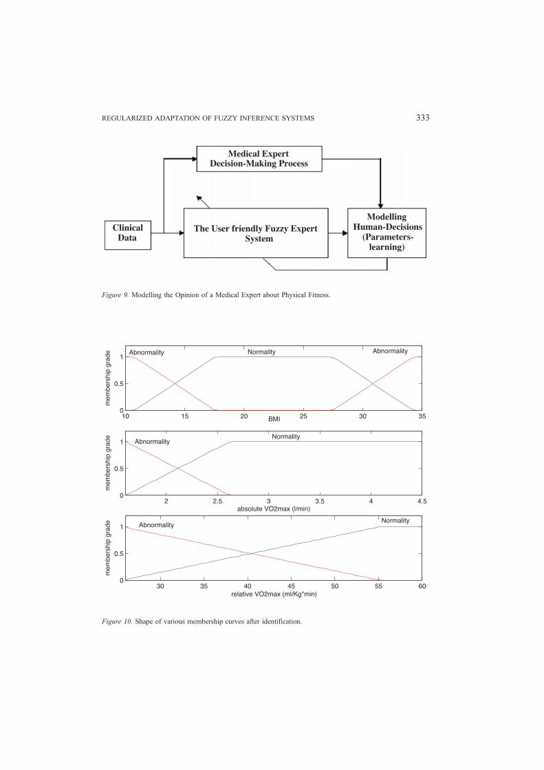
Figure 9. Modelling the Opinion of a Medical Expert about Physical Fitness.
Figure 10. Shape of various membership curves after identification.
REGULARIZED ADAPTATION OF FUZZY INFERENCE SYSTEMS 333
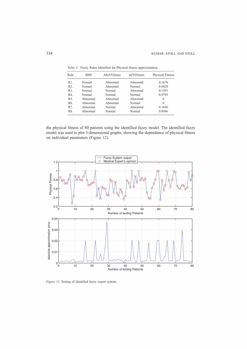
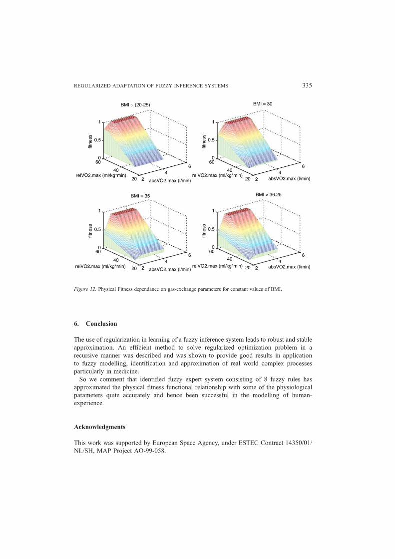
the physical fitness of 80 patients using the identified fuzzy model. The identified fuzzy
model was used to plot 3-dimensional graphs, showing the dependance of physical fitness
on individual parameters (Figure 12).
Table 3. Fuzzy Rules identified for Physical fitness approximation.
Rule BMI AbsVO2max relVO2max Physical Fitness
R1. Normal Abnormal Abnormal 0.1676
R2. Normal Abnormal Normal 0.6828
R3. Normal Normal Abnormal 0.1591
R4. Normal Normal Normal 0.9793
R5. Abnormal Abnormal Abnormal 0
R6. Abnormal Abnormal Normal 0
R7. Abnormal Normal Abnormal 0.1656
R8. Abnormal Normal Normal 0.8986
Figure 11. Testing of identified fuzzy expert system.
KUMAR, STOLL AND STOLL334
6. Conclusion
The use of regularization in learning of a fuzzy inference system leads to robust and stable
approximation. An efficient method to solve regularized optimization problem in a
recursive manner was described and was shown to provide good results in application
to fuzzy modelling, identification and approximation of real world complex processes
particularly in medicine.
So we comment that identified fuzzy expert system consisting of 8 fuzzy rules has
approximated the physical fitness functional relationship with some of the physiological
parameters quite accurately and hence been successful in the modelling of human-
experience.
Acknowledgments
This work was supported by European Space Agency, under ESTEC Contract 14350/01/
NL/SH, MAP Project AO-99-058.
Figure 12. Physical Fitness dependance on gas-exchange parameters for constant values of BMI.
REGULARIZED ADAPTATION OF FUZZY INFERENCE SYSTEMS 335
References
Babuska, R. (2000). ‘‘Construction of Fuzzy Systems-Interplay Between Precision and Transparency,’’ In Proc.
ESIT 2000. Aachen, 445–452.
Binder, A., H. W. Engl, C. W. Groetsch, A. Neubauer, and O. Scherzer. (1994). ‘‘Weakly Closed Nonlinear
Operators and Parameter Identification in Parabolic Equations by Tikhonov Regularization,’’ Appl. Anal. 55,
215–234.
Bodenhofer, U. and P. Bauer. (2000). ‘‘Towards an Axiomatic Treatment of Interpretability,’’ In Proc. IIZUKA2000.
Iizuka, 334–339 (October).
Burger, M., J. Haslinger and U. Bodenhofer. (2000). ‘‘Regularized Optimization of Fuzzy Controllers,’’ Technical
Report SCCH-TR-0056, Software Competence Center Hagenberg.
Burger, M., H. W. Engl, J. Haslinger, and U. Bodenhofer. (2002). ‘‘Regularized Data-Driven Construction of
Fuzzy Controllers,’’ J. Inverse and Ill-posed Problems 10, 319–344.
Engl, H. W., K. Kunisch, and A. Neubauer. (1989). ‘‘Convergence Rates for Tikhonov Regularization of Non-
linear Ill-Posed Problems’’ Inverse Problems 5, 523–540.
Engl, H. W., M. Hanke, and A. Neubauer. (1996). Regularization of Inverse Problems. Dordrecht: Kluwer
Academic Publishers.
Espinosa, J. and J. Vandewalle. (2000). ‘‘Constructing Fuzzy Models with Linguistic Integrity from Numerical
Data-AFRELI Algorithm,’’ IEEE Trans. Fuzzy Systems 8(5), 591–600 (October).
Jang, J.-S. R., C.-T. Sun and E. Mizutani. (1997). Neuro-Fuzzy and Soft Computing: A Computational Approach
to Learning and Machine Intelligence. Prentice Hall, Chapter 12, 345–360.
Lawson, C. L. and R. J. Hanson. (1995). Solving Least squares Problems. Philadelphia: SIAM Publications.
Nauck, D. and R. Kruse. (1999). ‘‘Obtaining Interpretable Fuzzy Classification Rules from Medical Data,’’
Artificial Intelligence in Medicine 16, 149–169.
Setnes, M., R. Babuka, and H. B. Verbruggen. (1998). ‘‘Rule-Based Modeling: Precision and Transparency,’’
IEEE Trans. Syst. Man Cybern.Part C: Applications and Reviews 28, 165–69.
Takagi, T. and M. Sugeno. (1985). ‘‘Fuzzy Identification of Systems and Its Applications to Modeling and
Control,’’ IEEE Trans. Syst. Man Cybern 15(1), 116–132.
Vainamo, K., S. Nissila, T. Makikallio, M. Tulppo and J. Roning. (1996). ‘‘Artificial Neural Network for Aerobic
Fitness Approximation,’’ International Conference on Neural Networks (ICNN96). Washington DC, USA (June
3–6).
Vainamo, K., T. Makikallio, M. Tulppo and J. Roning. (1998). ‘‘A Neuro-Fuzzy Approach to Aerobic Fitness
Classification: A Multistructure Solution to the Context-Sensitive Feature Selection Problem,’’ Proc. WCCI ‘98.
Anchorage, Alaska, USA, 797–802 (May 4–9).
Widrow, B. and M. A. Lehr. (1990). ‘‘30 Years of Adaptive Neural Networks: Perceptron, Madline and Back-
propagation,’’ Proceeding of the IEEE 78(9), 1415–1422.
Zadeh, L. A. (1973). ‘‘Outline of a New Approach to the Analysis of Complex Systems and Decision Processes,’’
IEEE Trans. Syst. Man Cybern 3(1), 28–44.
KUMAR, STOLL AND STOLL336