REGRESSION MODELS VS. VARIANCE MEASURES AS
STABILITY PARAMETERS OF SOME SOYBEAN
GENOTYPES
R. M. Akram1, W. M. Fares
2, A. M. EL-GARHY
1, A.A.M.Ashrie
1 Food Legume Crops Res. Dep., Field Crops Res. Inst., ARC, Giza.
2Central Lab. of Design & Stat. Analysis Res., ARC, Giza.
ABSTRACT
The presence of genotype × environment (G × E) interaction is a major
concern to plant breeder, since large interaction can reduce gains from selection and
complicate identification of surperior genotypes. Fifteen soybean genotypes were
grown in randomized complete block design with three replications at each of five
locations (Etay Elbarood, Gemmeiza, Sakha, Sids and Mallawy) through two
successive seasons ended in 2011. The objectives were to assess the yield
performance determine the magnitude of (G × E) interaction and investigate the
stability of the aimed genotypes using twelve stability statistics derived from two
types of statistical procedures (regression and variance approaches) . Also, Spearman
rank correlation coefficient principal components analysis and biplot graph were
applied to obtain good understanding of the interrelationships and overlapping among
the stability statistics used. The results showed highly significant mean squares for
genotypes, environments and (G × E) interaction indicating that the tested genotypes
exhibited different responses to environmental conditions. Also, the terms of
predictable (linear) and unpredictable (non - linear) interaction component were
highly significant which confirm that the tested soybean genotypes differed
considerably in their relative stability. The greatest seed yield was obtained by
genotype Giza 111 followed by H2L12, H30, DR101, H117, Giza21, H32 and H15L5
that surpassed the grand mean over the environments. It is evident that genotype Giza
111 in addition to its high yield, it was more stable one because it met the
assumptions of stable genotype as described by the stability models of Eberhart &
Rassell (1966), Tai (1971), Francis and Kannenberg (1978), Kang and Magari (1995)
and Shraan and Ghallab (2001). Hence, the genotype Giza111 maybe recommended
incorporating into a breeding stock in any future breeding program of soybean.
Considering the results of rank correlation, principal components analysis and biplot
graph, they showed the twelve stability statistics used could be grouped in four
distinct classes. The first class included the parameters of S2d, λ, W
2, σ
2 and S
2
because their perfect correlation. The parameters of RD, RDD, RHDDD and CV%
formed the elements of second class while the third class contained both of b and α
parameters. According to the highly significant association between both ΥS and
mean seed yield, they formed the correlated elements of the fourth class.
INTRODUCTION
Soybean (Glycine max L.) is one of the most important legume
crops that are considered a source of good quality protein in the diets of
people and also as valuable animal feed. Also, it requires no N fertilizer
owing to its ability to fix the atmospheric N and in rotation can improve
the N nutrition and yield of the subsequent cereal crop. Therefore, the
development of stable high yielding genotypes is a vital goal to increase
soybean area and production.
One of the essential final stages in most applied plant breeding
programs is the evaluation of the aimed genotypes over diversified
environments (years and locations). With quantitatively inherited traits,
for which heritabilities low, the yield performance of genotype often
varies from one environment to another, leading to a significant genotype
x environment (GxE) interaction. Whenever, the (GxE) interaction is
significant, the use of mean seed yield over environments as indicator of
genotype performance is questionable (Ablett et al, 1994). The combined
analysis of variance is only useful in estimating the existence,
significance and magnitude of stability. A genotype is considered to be
most stable one if it has a high mean yield and the ability to avoid
substantial fluctuations in yield when grown under diverse environments.
Many investigators among them Beaver and Johnson (1981), Radi et al
(1993), Ablett et al (1994), Al-Assily et al (1996) and (2002) described
the importance of (GxE) in stability analysis of soybean.
There are several statistical methods to measure stability by
modeling the (GxE) interaction. Most widely used methods, however, are
those based on regression models and variance measures.
The earliest form of regression statistics as stability parameter was
proposed by Yates and Cochran (1938) that was rediscovered by Finlay
and Wilkinson (1963) and then was improved by Eberhart and Russell
(1966). Two stability parameters similar to those of Eberhart and Russell
(1966) were also proposed by Tai (1971). According to the regression
approach, the stability is expressed in terms of 3 parameters being the
mean performance, the slope of regression line and the sum of squares
deviation from regression.
The statistics that parameterized the variance component measures
as stability parameters reflected the inconsistency of yield performance
across range of aimed environments or the contribution of each genotype
to the total (GxE) interaction. The famous parameters that fall into this
aspects of stability including the ecovalence (W2) proposed by Wricke
(1962) and then developed to two stability variance statistics (σ2 and S
2)
as described by Shukla (1972). The coefficient of variation (CV %) was
suggested by Francis and Kannenberg (1978). The yield stability (YS)
was proposed by Kang and Magari (1995) for simultaneous selection of
yield performance an d stability proper. Recently, Sharaan and Ghallab
(2001) provided three parallel statistics termed as RD, RDD RHDDD.
Although, many biometrical studies of stability models were
proposed, there is little attention or information available on the
consequences of using different stability statistics on the genotype ranks
in yield trials. Many authors discussed the associations among the
stability parameters (Becker 1981, Piepho and Lotito 1992, Duarte and
Zimmermann 1995, Sharaan and Ghallab 2001, Afiah et al 2002,
Mohebodini et al 2006, Dehghani et al 2008 and Zali et al 2011). They
found that several stability models probably measures the same stability
aspect due to the overlapping of computing their statistics. In Egypt, on
soybean, no references have been found about the previous point.
Therefore, the objectives of this work was to determine the stability
proper of seed yield in 15 soybean genotypes and to estimate Spearman
rank correlation coefficient among 12 stability parameters used.
MATERIALS AND METHODS
The current investigation was carried out during 2010 and 2011
growing seasons in five different research stations (combined 10
environments) to evaluate the yield performance of 15 soybean
genotypes. The five locations were chosen to represent the most climatic
conditions, soil types, degree of temperature and other agro-climatic
factors that likely to be encountered upon soybean growing through
Egypt. They were Etay Elbarood, Sakha, Gemmeiza, Sids and Mallawy.
A detailed description of the code, name, pedigree, maturity group,
flower color and origin of the tested genotypes are presented in Table (1).
Randomized complete block design with three replications was
used. The experimental plot consisted of six ridges, 4 m long and 70 cm
apart. The other agricultural practices were applied as per
recommendation to research the maximum seed yield for each respective
location. At harvest, seed yield was calculated from the three central
ridges of each plot and then transformed to the unit of kg/fed.
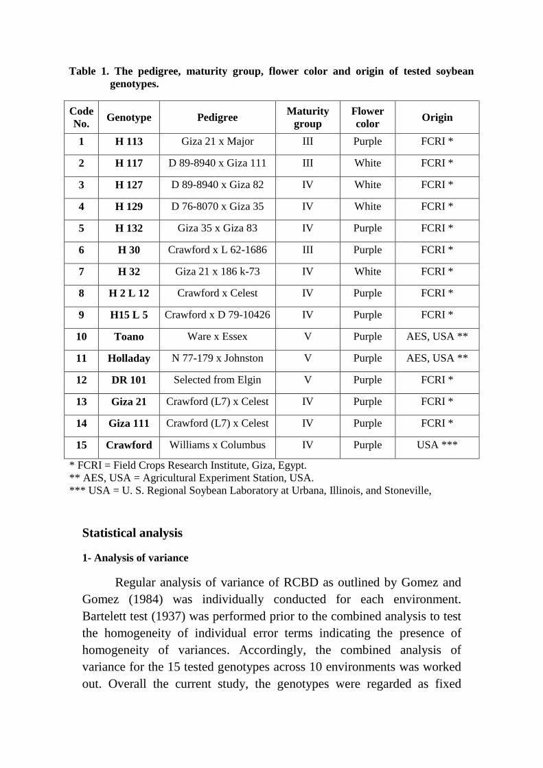
Table 1. The pedigree, maturity group, flower color and origin of tested soybean
genotypes.
Code
No. Genotype Pedigree
Maturity
group
Flower
color Origin
1 H 113 Giza 21 x Major III Purple FCRI *
2 H 117 D 89-8940 x Giza 111 III White FCRI *
3 H 127 D 89-8940 x Giza 82 IV White FCRI *
4 H 129 D 76-8070 x Giza 35 IV White FCRI *
5 H 132 Giza 35 x Giza 83 IV Purple FCRI *
6 H 30 Crawford x L 62-1686 III Purple FCRI *
7 H 32 Giza 21 x 186 k-73 IV White FCRI *
8 H 2 L 12 Crawford x Celest IV Purple FCRI *
9 H15 L 5 Crawford x D 79-10426 IV Purple FCRI *
10 Toano Ware x Essex V Purple AES, USA **
11 Holladay N 77-179 x Johnston V Purple AES, USA **
12 DR 101 Selected from Elgin V Purple FCRI *
13 Giza 21 Crawford (L7) x Celest IV Purple FCRI *
14 Giza 111 Crawford (L7) x Celest IV Purple FCRI *
15 Crawford Williams x Columbus IV Purple USA ***
* FCRI = Field Crops Research Institute, Giza, Egypt.
** AES, USA = Agricultural Experiment Station, USA.
*** USA = U. S. Regional Soybean Laboratory at Urbana, Illinois, and Stoneville,
Mississipi.
Statistical analysis
1- Analysis of variance
Regular analysis of variance of RCBD as outlined by Gomez and
Gomez (1984) was individually conducted for each environment.
Bartelett test (1937) was performed prior to the combined analysis to test
the homogeneity of individual error terms indicating the presence of
homogeneity of variances. Accordingly, the combined analysis of
variance for the 15 tested genotypes across 10 environments was worked
out. Overall the current study, the genotypes were regarded as fixed
effects whereas environments (combinations of years x locations)
considered as random effects.
The detection of significant interaction between genotypes and
environments (GxE) enabled us to study the stability of yield
performance for the tested genotypes. Moreover, Zobel et al (1988)
proposed using Tukey test (1949) that separates one degree of freedom
for non additive component to exam the presence of multiplicative (GxE)
interaction in the two way data. The significance of non additive
component was considered another justification to study the stability.
2- Stability analyses
Seven widely used methods of stability were applied to
differentiate the studied soybean genotypes and to exploit the available
information from these statistics for obtaining stable genotypes to be
release as materials to be incorporated in the breeding programs of
soybean. According to the mathematical concept, the used stability
methods were placed into two main groups namely; regression model and
variance measures. Under the regression approach, the genotype is
considered to be stable if its response to environmental index is parallel to
the mean response of ell genotypes in the trial in addition to its deviation
from regression model is minimum. This group comprised two stability
methods being Eberhart & Russell (1966) and Tai (1971).
Concerning the group of stability variance procedure, a genotype
with minimum variance measure across different environments was
considered to be stable. The five stability models of Wricke (1962),
Shukla (1972), Francis & Kannenberg (1978), Kang & Magari (1995) and
Sharaan & Ghallab (2001) followed the last group.
Over the two groups of stability parameters, the high yielding
ability of a genotype is a precondition for stability concept. The
computations of the current procedures of stability were mentioned in
details through many preceding papers. So, brief description of each
follows.
The regression model suggested by Eberhart & Russell (1966)
provides the linear regression coefficient, b, as indication of the response
of the genotype to the environmental index and the deviation from
regression mean square, S2d, as a criterion of stability as suggested by
Beker and Leon (1988). If the regression coefficient (b value) is not
significantly different from unity, the genotype is adapted in all
environments. Genotypes with b >1.0 are more responsive to high
yielding environments, whereas any genotype with b lower than 1.0 is
adapted to low yielding environments. In the expression of S2d, we did
not subtract S2e/r (pooled error), since this value is constant for all
genotypes and it does not alter rank orders (Duarte and Zimmermann,
1995).
A two stability statistics method similar to that of Eberhart &
Russell (1966) was also proposed by Tai (1971). The first statistic is α
that measure the linear response of environmental effects while the
second one is λ that reflects the deviation from linear response in terms of
magnitude of the error variance. The two components are defined as
genotypic stability parameters. In fact, the parameters of α and λ can be
regarded as modified form of b and S2d, respectively. A perfectly stable
genotype would not change its performance from one environment one to
another. This is equivalent to stating α = -1 and λ = 1. Because the perfect
stable genotypes rarely are exist, the plant breeder will have to be
satisfied with statistically admissible level of stability. The values (α = 0
& λ = 1) will be referred to as average stability, whereas the values (α > 0
& λ = 1) will be as below average stability, however, the values (α < 0 &
λ = 1) will be referred to as above average stability.
Ecovalence stability index, W2 or the contribution of a genotype to
the GxE interaction sum of squares which was proposed by Wricke
(1962) has been utilized in the present study. Because the value of W2
is
expressed as sum of squares, no means of testing the significance of W2
for each genotype. In accordance, the genotype has minimum value of the
parameter W2 was considered stable.
Shukla (1972) developed an unbiased estimate of stability variance
termed as σ2. The Shukla method can be extended to us a covariate to
overcome the linear effect from GxE interaction. The remainder of GxE
interaction variance can be assigned to each genotype as second stability
parameter S2. The test of significance is available for the two stability
variance parameters (σ2 and S
2) against the error variance.
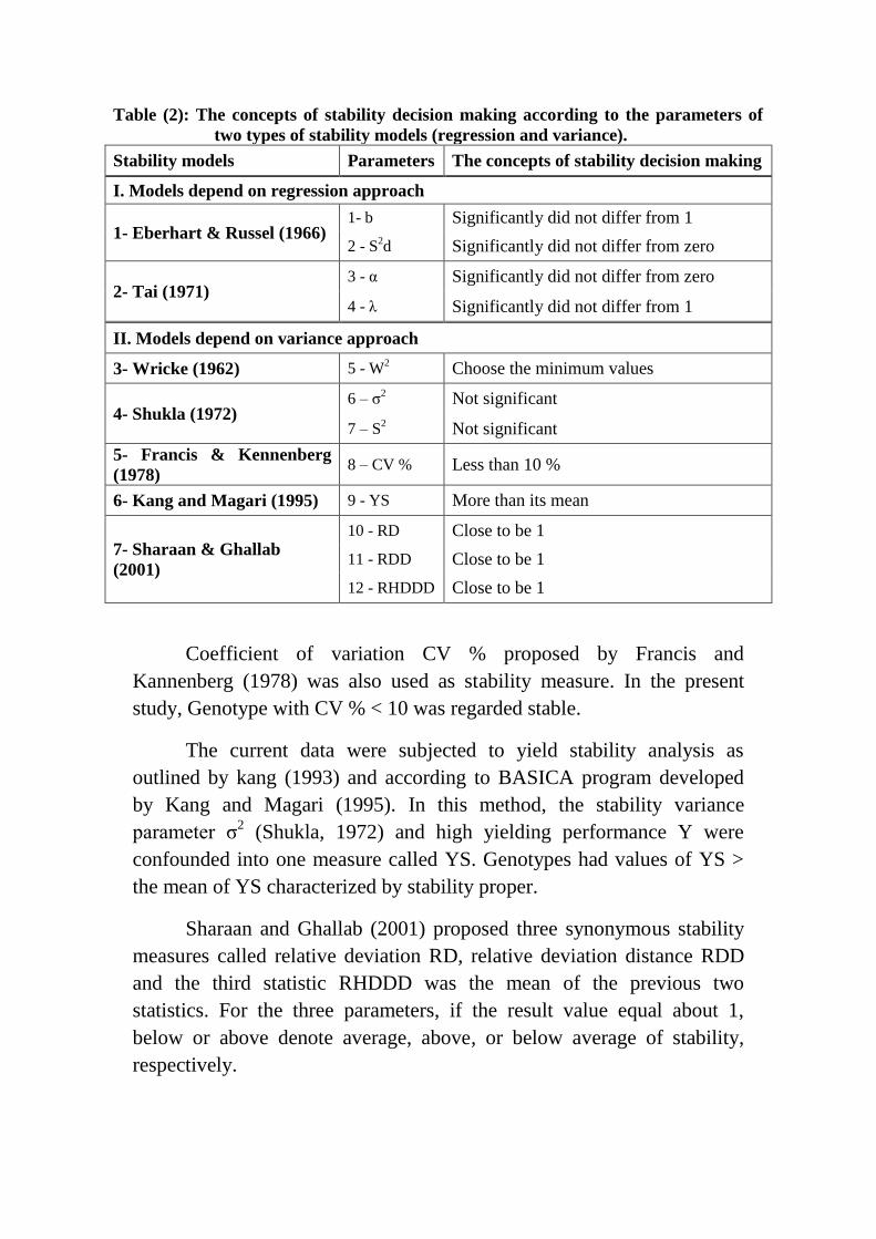
Table (2): The concepts of stability decision making according to the parameters of
two types of stability models (regression and variance).
Stability models Parameters The concepts of stability decision making
I. Models depend on regression approach
1- Eberhart & Russel (1966) 1- b Significantly did not differ from 1
2 - S2d Significantly did not differ from zero
2- Tai (1971) 3 - α Significantly did not differ from zero
4 - λ Significantly did not differ from 1
II. Models depend on variance approach
3- Wricke (1962) 5 - W2 Choose the minimum values
4- Shukla (1972) 6 – σ
2 Not significant
7 – S2 Not significant
5- Francis & Kennenberg
(1978) 8 – CV % Less than 10 %
6- Kang and Magari (1995) 9 - YS More than its mean
7- Sharaan & Ghallab
(2001)
10 - RD Close to be 1
11 - RDD Close to be 1
12 - RHDDD Close to be 1
Coefficient of variation CV % proposed by Francis and
Kannenberg (1978) was also used as stability measure. In the present
study, Genotype with CV % < 10 was regarded stable.
The current data were subjected to yield stability analysis as
outlined by kang (1993) and according to BASICA program developed
by Kang and Magari (1995). In this method, the stability variance
parameter σ2 (Shukla, 1972) and high yielding performance Y were
confounded into one measure called YS. Genotypes had values of YS >
the mean of YS characterized by stability proper.
Sharaan and Ghallab (2001) proposed three synonymous stability
measures called relative deviation RD, relative deviation distance RDD
and the third statistic RHDDD was the mean of the previous two
statistics. For the three parameters, if the result value equal about 1,
below or above denote average, above, or below average of stability,
respectively.
The concepts of stability decision making according to the
parameters of two types of stability models (regression and variance) are
presented in Table (2).
Although, the use of stability parameters belonging to various
concepts may lead to different rankings of genotypes in their stability,
there is little attention and information available on the similarity among
these stability parameters as well as on the consequences and
effectiveness of the utilization of different parameters for an ordering
genotypes.
To give overall picture emerges the interrelationships and
overlapping among the used stability parameters, Spearman rank
correlation coefficients between all pairs of the twelve parameters as well
as mean seed yield were computed (Duarte and Zimmermann, 1995). The
rank correlation was used instead of ordinary Pearson coefficient of
correlation because the stability parameters can not be assumed to be
normally distributed (Becker, 1981).
Principal component (PC) analysis based on the rank correlation
matrix was also performed for grouping the similar stability parameters in
different classes. For better visualization, the firest two principal
components were graphically plotted against each other using biplot
graph as described by Mohebodinin et al (2006).
RESULTS AND DISCUSSION
The regular combined analysis of variance for seed yield of the 15
soybean genotypes (G) across the 10 environments (E) and their (GxE)
interaction (data not tabulated). These results indicated differential
genotypic behavior as well as wide range of variability across locations
and years. The highly significant effect of (GxE) interaction confirmed
the effect that the tested genotypes did not react in similar way to change
through environments. In accordance, the data of mean seed yield through
the studied environments were subjected to stability analysis. On the
other hand, the significance of non-additive component of the two way
interaction data (Tukey test, 1949) gave other justification to study the
stability proper. Radi et al (1993) found large magnitude of (GxE)
interaction and concluded that the soybean genotypes fluctuated in the
rank performance for seed yield across the aimed environments in their
study.
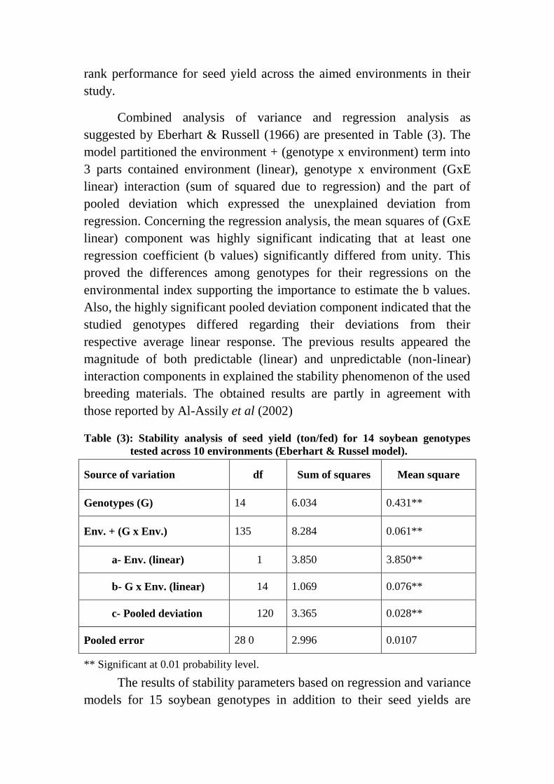
Combined analysis of variance and regression analysis as
suggested by Eberhart & Russell (1966) are presented in Table (3). The
model partitioned the environment + (genotype x environment) term into
3 parts contained environment (linear), genotype x environment (GxE
linear) interaction (sum of squared due to regression) and the part of
pooled deviation which expressed the unexplained deviation from
regression. Concerning the regression analysis, the mean squares of (GxE
linear) component was highly significant indicating that at least one
regression coefficient (b values) significantly differed from unity. This
proved the differences among genotypes for their regressions on the
environmental index supporting the importance to estimate the b values.
Also, the highly significant pooled deviation component indicated that the
studied genotypes differed regarding their deviations from their
respective average linear response. The previous results appeared the
magnitude of both predictable (linear) and unpredictable (non-linear)
interaction components in explained the stability phenomenon of the used
breeding materials. The obtained results are partly in agreement with
those reported by Al-Assily et al (2002)
Table (3): Stability analysis of seed yield (ton/fed) for 14 soybean genotypes
tested across 10 environments (Eberhart & Russel model).
Source of variation df Sum of squares Mean square
Genotypes (G) 14 6.034 0.431**
Env. + (G x Env.) 135 8.284 0.061**
a- Env. (linear) 1 3.850 3.850**
b- G x Env. (linear) 14 1.069 0.076**
c- Pooled deviation 120 3.365 0.028**
Pooled error 28 0 2.996 0.0107
** Significant at 0.01 probability level.
The results of stability parameters based on regression and variance
models for 15 soybean genotypes in addition to their seed yields are
shown in Table (4). Significant differences among genotypes in terms of
seed yield were determined. The highest seed yield was obtained by
genotype Giza 111 recording 1.85 (ton/fed) followed by genotypes
H2L12, H30, DR101, H117, Giza 21, H32, H15L5 and Holladay that
surpassed the overall mean recording 1.82, 1.72, 1.69, 1.66, 1.63, 1.61,
1.57 and 1.55 ton/fed.
According to the parameters of Eberhart & Russell model,
regression coefficients ranged from 0.09 to 1.97 indicating that genotypes
already had different responses to environmental changes. The values of
regression coefficient (b) did not significantly differ from unity for all
tested genotypes except for genotypes H113, H129, H2L12, Toano AND
Holladay. The values of deviation from regression (S2d) were
significantly different from zero for all genotypes except for genotypes
DR101, Giza21, Giza111 and Crawford. It is evidence that both
genotypes Giza21 and Giza111 had values of b and S2d did not
significantly differ from unity and zero, respectively. Moreover, they had
mean performance exceeded the mean of all genotypes. Therefore,
genotypes Giza21 and Giza111 was considered phenotypically stable
since it had the properties of the stable genotype as described by Eberhart
& Russell (1966) model.
On the other hand, genotypes H2L12, Holladay and DR101 would
be adapted to low yielding environments since they had b values
significantly less than unity in addition their seed yields exceeded the
overall mean.
With regard to genotypic stability as outlined by Tai (1971), the
estimates of α and λ are displayed in Table (4) and graphically illustrated
in Fig. (1).The results revealed that the genotypes H30, H32, Giza21,
Giza111 and Crawford were spotted in the average stability area
considering probability level equal 0.05. Only, DR101 had degree of
above average stability. Fortunately, the seed yield of these genotypes
exceeds the mean of all genotypes except Crawford indicating their
importance as a breeding stock in any further soybean breeding program
for satisfying stable high yielding genotypes.
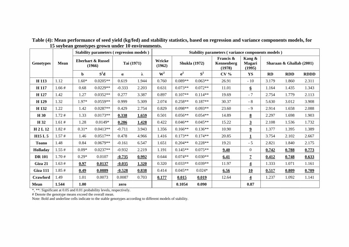
Table (4): Mean performance of seed yield (kg/fed) and stability statistics, based on regression and variance components models, for
15 soybean genotypes grown under 10 environments.
Genotypes Mean
Stability parameters ( regression models ) Stability parameters ( variance components models )
Eberhart & Russel
(1966) Tai (1971)
Wricke
(1962) Shukla (1972)
Francis &
Kennenberg
(1978)
Kang &
Magari
(1995)
Sharaan & Ghallab (2001)
b S2d α λ W
2 σ
2 S
2 CV % YS RD RDD RDDD
H 113 1.12 1.60* 0.0205** 0.619 1.944 0.760 0.089** 0.063** 26.91 - 10 3.179 1.860 2.311
H 117 1.66 # 0.68 0.0229** -0.333 2.203 0.631 0.073** 0.072** 11.01 6 1.164 1.435 1.343
H 127 1.42 1.27 0.0352** 0.277 3.387 0.897 0.107** 0.114** 19.69 - 7 2.754 1.779 2.113
H 129 1.32 1.97* 0.0559** 0.999 5.309 2.074 0.258** 0.187** 30.37 - 8 5.630 3.012 3.908
H 132 1.22 1.42 0.0287** 0.429 2.754 0.829 0.098** 0.093** 23.60 - 9 2.914 1.658 2.088
H 30 1.72 # 1.33 0.0173** 0.338 1.659 0.501 0.056** 0.054** 14.89 8 2.297 1.698 1.903
H 32 1.61 # 1.28 0.0149* 0.286 1.428 0.422 0.046** 0.045** 15.22 3 2.108 1.536 1.732
H 2 L 12 1.82 # 0.31* 0.0413** -0.711 3.943 1.356 0.166** 0.136** 10.90 9 1.377 1.395 1.389
H15 L 5 1.57 # 1.46 0.0517** 0.478 4.966 1.416 0.173** 0.174** 20.85 1 3.754 2.102 2.667
Toano 1.48 0.84 0.0679** -0.161 6.547 1.651 0.204** 0.228** 19.21 - 5 2.821 1.840 2.175
Holladay 1.55 # 0.09* 0.0237** -0.932 2.219 1.191 0.145** 0.075** 9.40 0 0.742 0.788 0.773
DR 101 1.70 # 0.29* 0.0107 -0.735 0.992 0.644 0.074** 0.030** 6.41 7 0.412 0.748 0.633
Giza 21 1.63 # 0.97 0.0137 -0.035 1.320 0.320 0.033** 0.039** 11.97 4 1.333 1.071 1.161
Giza 111 1.85 # 0.49 0.0889 -0.528 0.838 0.414 0.045** 0.024* 6.56 10 0.517 0.809 0.709
Crawford 1.49 1.01 0.0073 0.0087 0.703 0.177 0.015 0.019 12.64 4 1.237 1.092 1.141
Mean 1.544 1.00 zero 0.1054 0.090 0.87
*, **: Significant at 0.05 and 0.01 probability levels, respectively.
# Denote the genotype means exceed the overall mean.
Note: Bold and underline cells indicate to the stable genotypes according to different models of stability.
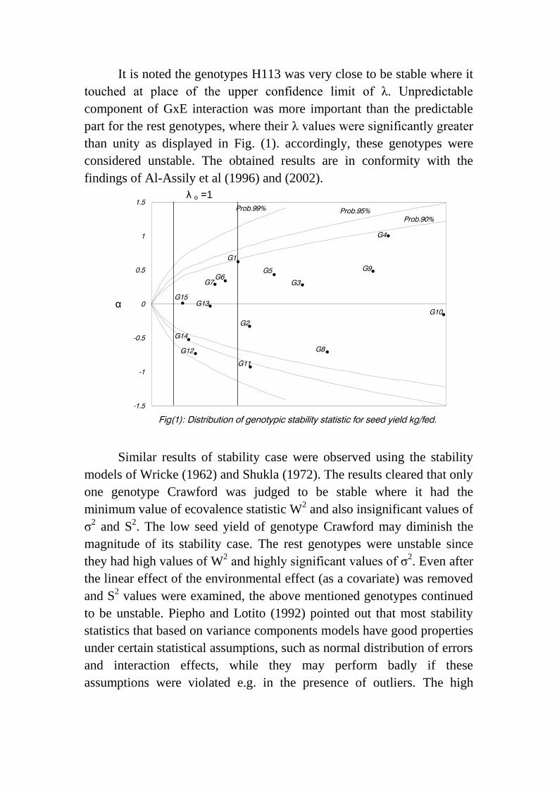
It is noted the genotypes H113 was very close to be stable where it
touched at place of the upper confidence limit of λ. Unpredictable
component of GxE interaction was more important than the predictable
part for the rest genotypes, where their λ values were significantly greater
than unity as displayed in Fig. (1). accordingly, these genotypes were
considered unstable. The obtained results are in conformity with the
findings of Al-Assily et al (1996) and (2002).
Similar results of stability case were observed using the stability
models of Wricke (1962) and Shukla (1972). The results cleared that only
one genotype Crawford was judged to be stable where it had the
minimum value of ecovalence statistic W2 and also insignificant values of
σ2 and S
2. The low seed yield of genotype Crawford may diminish the
magnitude of its stability case. The rest genotypes were unstable since
they had high values of W2 and highly significant values of σ
2. Even after
the linear effect of the environmental effect (as a covariate) was removed
and S2 values were examined, the above mentioned genotypes continued
to be unstable. Piepho and Lotito (1992) pointed out that most stability
statistics that based on variance components models have good properties
under certain statistical assumptions, such as normal distribution of errors
and interaction effects, while they may perform badly if these
assumptions were violated e.g. in the presence of outliers. The high
α
1 =o λ
values of CV % for some tested genotypes (for example, genotype H129
recorded CV % = 30.37) supported the earlier remark.
On the other hand, concerning the values of CV % as stability
statistics according to Francis and Kannenberg (1978), the results
declared that genotypes Holladay, DR101 and Giza111 recorded CV
values less than 10 exhibiting their stability. Moreover, the three
genotypes had seed yield surpassed the grand mean yield. It is easy to
discover that the obtained results of the three stability measures (RD,
RDD and RHDDD) of the model supposed by Sharaan and Ghallab
(2001) were exactly similar to those obtained by using CV % as a
stability criterion. In fact, the aforementioned three stability measures
were considered substitutes of each other.
Nine genotypes out of 15 were characterized by stability plus high
performance of seed yield according to Kang and Magari (1995) method
as shown in Table (4). These genotypes were H117, H30, H32, H2L12,
H15L5, DR101, Giza21, Giza111 and Crawford. They had YS value was
greater than the mean of YS, so, it is judged to be stable.
It is clearly appeared that great number of stable genotypes (9 out
of 15) was only chosen by the model of Kang and Magari (1995)
compared to the other studied stability models. One of the reasons is the
non-parametric concept of measuring the YS. Also, the complementally
relationship between the two components of computing YS (yield and
Shukla stability statistic σ2) may be another cause. For example, although
genotypes H117, H30, H32, H2L12, H15L5, DR101, Giza21 and
Giza111 had highly significant values of σ2, they were stable considering
YS statistic because their high yields. In contrast, the stability of
Crawford using YS statistic may be returned to the insignificant value of
σ2
irrespective of its low yield. So, the stability model of Kang and
Magari (1995) may be less effective compared to the other studied
parametric model. Piepho and Lotito (1992) reported that the non-
parametric models of stability would be used when the necessary
assumptions for the parametric stability models are violated.
In summary, it is evidence that genotype Giza111 in addition to its
high yield, it was more stable one because it met the assumptions of
stable genotype as described by 9 out of the 12 stability statistics used
(Table 4). Therefore, this genotype may be taken in account as breeding
material stock in any future breeding program of soybean Al-Assily et al
(2002). It is worthy to mention that further stability reevaluating study of
the unstable genotypes is a necessary step to get more confidence
conclusion about them (Lin et al, 1986).
Spearman coefficients of rank correlation (r) among the used
stability parameters as well as mean seed yield are presented in Table (5).
In this part of the study, we aim to explore the stability parameters that
are closely related in sorting out the relative stability of the tested
soybean genotypes. So, we would only discuss the stability parameters
that are highly significant correlated with r value greater than 0.8.
When perfect correlation coefficient (r=1) was obtained between
two stability parameters, then they would be identical parameters.
However, if the association between two stability parameters was only
very strong (highly significant with (0.8 < r <1), then, the two parameters
would be as equivalent.
The results clearly appeared the mean seed yield was independent
from most stability parameters except CV % and YS. The negative
association between mean seed yield and CV % (-0.8**) indicate that the
high yielding genotypes were less affected by the environmental
variation. The high positive correlation between mean seed yield and YS
(0.97**) is not surprise because mean seed yield is a basic component in
computing the parameters of YS suggesting that using YS as a stability
parameter may not provide more information than mean seed yield its
self. Our results are particularly consistent with these published by others
(Duarte and Zimmermann, 1995; Sharaan and Ghallab, 2001; Akcura et
al, 2006; Mohebodini et al, 2006, Dehghani et al, 2008 and Zali et al,
2011).
In fact, the results of correlation among stability parameters
reported in the literature differ in value. This result is expected, because
the results would depend on the tested genotypes and environmental
range study.
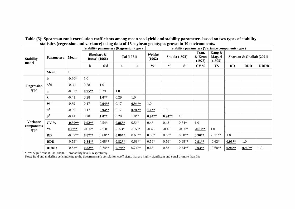
Table (5): Spearman rank correlation coefficients among mean seed yield and stability parameters based on two types of stability
statistics (regression and variance) using data of 15 soybean genotypes grown in 10 environments.
Stability
model
Parameters Mean
Stability parameters (Regression type ) Stability parameters (Variance components type )
Eberhart &
Russel (1966) Tai (1971)
Wricke
(1962) Shukla (1972)
Fran.
& Kenn
(1978)
Kang &
Magari
(1995)
Sharaan & Ghallab (2001)
b S2d α λ W
2 σ
2 S
2 CV % YS RD RDD RDDD
Mean 1.0
Regression
type
b -0.60* 1.0
S2d -0..41 0.28 1.0
α -0.53* 0.95** 0.29 1.0
λ -0.41 0.28 1.0** 0.29 1.0
Variance
components
type
W2 -0.39 0.17 0.94** 0.17 0.94** 1.0
σ2 -0.39 0.17 0.94** 0.17 0.94** 1.0** 1.0
S2 -0.41 0.28 1.0** 0.29 1.0** 0.94** 0.94** 1.0
CV % -0.80** 0.92** 0.54* 0.86** 0.54* 0.43 0.43 0.54* 1.0
YS 0.97** -0.60* -0.50 -0.53* -0.50* -0.48 -0.48 -0.50* -0.81** 1.0
RD -0.67** 0.87** 0.68** 0.80** 0.68** 0.58* 0.58* 0.68** 0.96** -0.71** 1.0
RDD -0.59* 0.84** 0.68** 0.82** 0.68** 0.56* 0.56* 0.68** 0.91** -0.62* 0.95** 1.0
RDDD -0.63* 0.82** 0.74** 0.79** 0.74** 0.63 0.63 0.74** 0.93** -0.68** 0.98** 0.99** 1.0
*, **: Significant at 0.05 and 0.01 probability levels, respectively.
Note: Bold and underline cells indicate to the Spearman rank correlation coefficients that are highly significant and equal or more than 0.8.
Concerning the relationship among stability parameters that depend
on regression approach (b, S2d and α, λ), the results showed highly
significant positive association (0.95**) between b and α while perfect
correlation (r=1**) was obtained between the parameters of S2d and λ
indicating that any one of the two stability models (Eberhart & Russell
1966 or Tai 1971) could be used as a substitute for the second in GxE
study of soybean. But, the model of Tai (1971) is preferred because it had
a genotypic concept of stability. On the other hand, Tai (1971)
mathematically proved that both α and λ are functions of b and S2d,
respectively. These findings are in agreement with these reported by Tai,
1971 Afiah et al, 2002, Akcura et al, 2006 Mohebodini et al, 2006 and
Dehghani et al, 2008.
With regard to the relationship among the stability parameters that
depend on variance measures, it is noted perfect positive correlation
(r=1**) between the parameters of W2 and σ
2 while the association
between S 2
was highly significant. Accordingly, the magnitude of σ2 and
W2 as stability parameters was about equal (identical parameters) where
the relative rankings of genotypes for the two parameters were exactly the
same. This requires that a decision must be made which of them should
be used as a stability variance parameter. The ability to test the
significance of σ2
plus the possibility to take one or more covariates into
account producing more information as S2
parameter supported the
direction of using Shukla parameters (σ2 and S
2). Because S
2 is
mathematically derived from σ2, so, the association between them was
very strong (0.94**). These results are similar to those obtained by kang
and Miller (1984), Lin et al (1986) and Akcura et al (2006).
Also, there was highly significant association between CV % and
each of RD, RDD and RHDDD indicating that they measured similar
aspects of stability. Therefore, it is possible to use only one of them as a
measure of stability.
According to the interrelationships among the parameters of RD,
RDD and RHDDD, they were strongly associated with each other. This
may be returned to the similarity of their computation bases. The earlier
results of Sharaan and Ghallab (2001) and Afiah et al (2002) were in
harmony with the current findings.
Considering the correlation among the parameters of the two
models of stability (regression and variance procedures), it is noted that
both b and α had high significant associations with each of RD, RDD and
RHDDD. Also, there was perfect correlation between each of S2d and λ
performance side and S2 in the other side while their associations with
each of W2 and σ2 were highly significant.
The previous results suggested that the simultaneous utilization of
the strongly or perfectly correlated parameters of stability is not
justifiable and one of them would probably be sufficient or enough.
These findings were in line with those obtained by Duarte and
Zimmermann (1995),Sharaan and Ghallab (2001), Afiah et al (2002),
Akcura et al (2006), Mohebodini et al (2006) and Dehghani et al (2008).
To be more aware about the interrelationships among the 12
stability parameters, principal components (PC) analysis based on the
Spearman rank correlation matrix, was performed. For best Visualization,
the loadings of the first two principal components were plotted against
each other. The results of principal components analysis were presented
in Table (6) and diagrammatically displayed as biplot graph of PC1 and
PC2 in Figure (2).
The sign of the first principal component PC1 indicate to the
direction of associations among the stability parameters while the
absolute values of the PC2 grouped the stability parameters into similar
classes. Considering the results of Table (6) and Figure (2), it is noted the
first two PC`s shared by 99.8 % (82.6 and 17.1 % by PC1 and PC2,
respectively) of the variance structure. The high value of the variance
explained by principal components analysis may be attributed to the
perfect association among some stability parameters as reported in Table
(5).
The principal components analysis or the biplot graph of PC1 and
PC2 axes distinguished the 12 stability parameters into 4 different groups
or classes
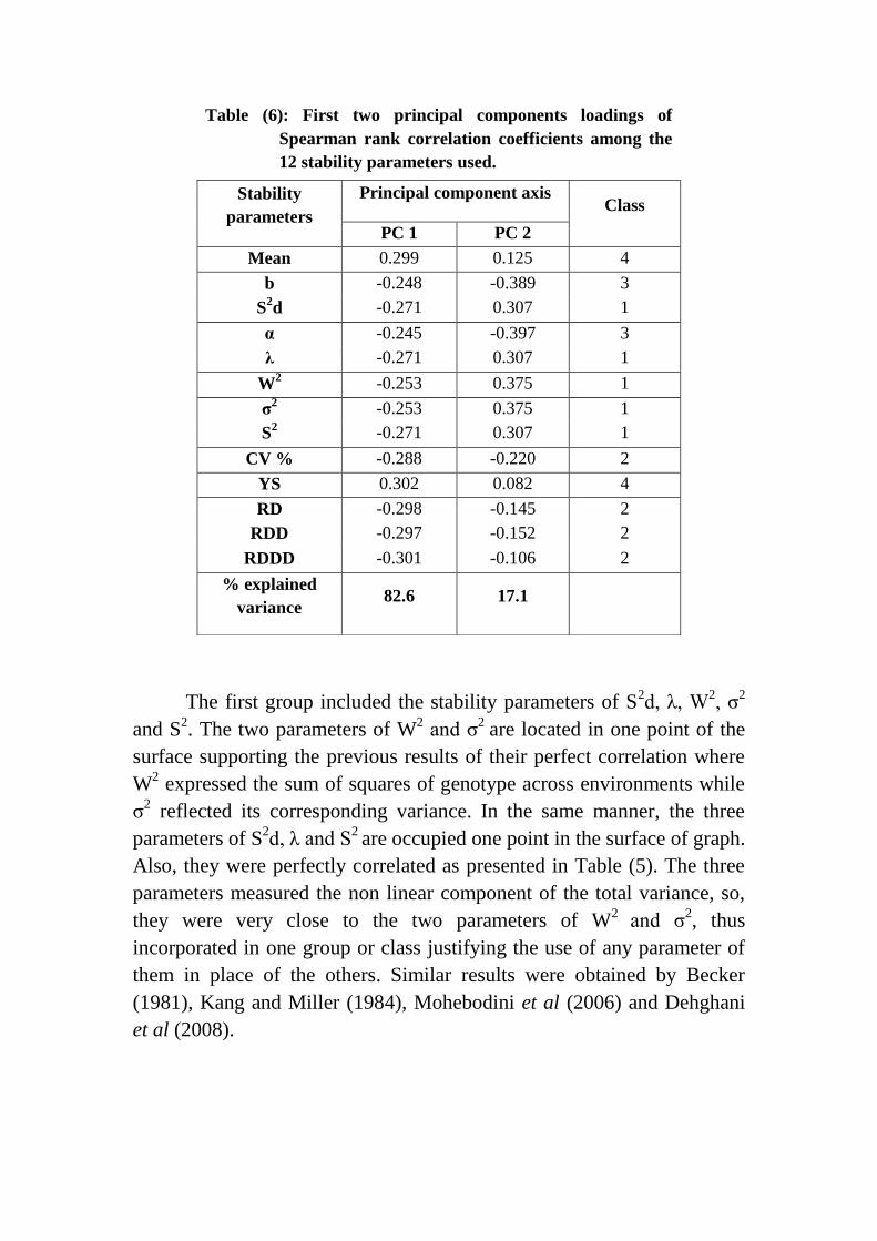
The first group included the stability parameters of S2d, λ, W
2, σ
2
and S2. The two parameters of W
2 and σ
2 are located in one point of the
surface supporting the previous results of their perfect correlation where
W2 expressed the sum of squares of genotype across environments while
σ2 reflected its corresponding variance. In the same manner, the three
parameters of S2d, λ and S
2 are occupied one point in the surface of graph.
Also, they were perfectly correlated as presented in Table (5). The three
parameters measured the non linear component of the total variance, so,
they were very close to the two parameters of W2
and σ2, thus
incorporated in one group or class justifying the use of any parameter of
them in place of the others. Similar results were obtained by Becker
(1981), Kang and Miller (1984), Mohebodini et al (2006) and Dehghani
et al (2008).
Table (6): First two principal components loadings of
Spearman rank correlation coefficients among the
12 stability parameters used.
Stability
parameters
Principal component axis Class
PC 1 PC 2
Mean 0.299 0.125 4
b -0.248 -0.389 3
S2d -0.271 0.307 1
α -0.245 -0.397 3
λ -0.271 0.307 1
W2 -0.253 0.375 1
σ2 -0.253 0.375 1
S2 -0.271 0.307 1
CV % -0.288 -0.220 2
YS 0.302 0.082 4
RD -0.298 -0.145 2
RDD -0.297 -0.152 2
RDDD -0.301 -0.106 2
% explained
variance 82.6 17.1
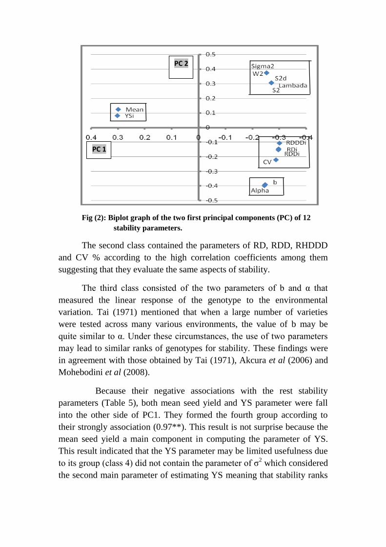
Fig (2): Biplot graph of the two first principal components (PC) of 12
stability parameters.
The second class contained the parameters of RD, RDD, RHDDD
and CV % according to the high correlation coefficients among them
suggesting that they evaluate the same aspects of stability.
The third class consisted of the two parameters of b and α that
measured the linear response of the genotype to the environmental
variation. Tai (1971) mentioned that when a large number of varieties
were tested across many various environments, the value of b may be
quite similar to α. Under these circumstances, the use of two parameters
may lead to similar ranks of genotypes for stability. These findings were
in agreement with those obtained by Tai (1971), Akcura et al (2006) and
Mohebodini et al (2008).
Because their negative associations with the rest stability
parameters (Table 5), both mean seed yield and YS parameter were fall
into the other side of PC1. They formed the fourth group according to
their strongly association (0.97**). This result is not surprise because the
mean seed yield a main component in computing the parameter of YS.
This result indicated that the YS parameter may be limited usefulness due
to its group (class 4) did not contain the parameter of σ2 which considered
the second main parameter of estimating YS meaning that stability ranks
2PC
1PC
of genotypes using YS parameter may be more influenced by mean seed
yield than σ2.
Based on the aforementioned discussion, it could be safely
recommended to use stability parameters that followed different classes
to avoid the risk of measuring the same aspects of stability.
Overall the study, the stability statistics of regression approach
may be preferable over those of variance procedure because they give
more information as the shape of the response of genotype to
environmental index using b or α as well as the deviation from linear
regression using S2d or λ. Moreover, the result of regression approach
may possibly to be supported by the coefficient of determination (R2) as a
third parameter of stability according to Pinthus (1973). To satisfy more
reliable regression statistics as stability parameters, the number of
environments used must be adequate and represent a pattern of wide
range and relatively good distribution over the entire growing area.
Finally, the current study suggests that the stability analysis
effectively share with supplementary information on the performance of
new soybean selections prior to release for commercial field cultivation
and can increase the efficiency of cultivar development programs.
. REFERENCES
Ablett, G. R., R. I. Buzzell, W.D. Beversdorf and O.B. Allen (1994).
Comparative stability of indeterminate and semi determinate
soybean lines. Crop Sci., 34(2): 347-351.
Afiah, S. A. N., N. A. Mohamed, S. A. Omar and H. Kh. Hassan
(2002). Performance and stability of newly bred wheat genotypes
under rained and saline environments. Egyptian J. Desert Res.,
52(2): 299-316.
Akura, M., Y. Kaya, S. Taner and R. Ayranci (2006). Parametric
stability analyses for grain yield of durum wheat. Plant Soil
Environ, 52: 254-261.
Al-Assily, Kh. A., S. M. Nasr and Kh. A. Ali (1996). Genotype ×
environment interaction, yield stability and adaptability for
soybean (Glycine max L.). J. Agric. Sci. Mansoura Univ., 21:
3779-3789.
Al-Assily, Kh. A., S. R. Saleeb, S. H. Mansour and M.S. Mohamed
(2002). Stability parameters for soybean genotypes as criteria for
response to environmental conditions. Minufia J. Agric. Res.,
27(2): 169-180.
Bartle, M.S. (1937). Some example of statistical methods of research in
agricultural and applied biology. Jour. Roy. Stat. Soc. Suppl., 4:
137-183.
Beaver, J. S. and R. R. Jonson (1981). Yield stability of determinate
and indeterminate soybeans adapted to the Northern United
States. Crop Sci., 21: 449-453.
Beker, H.C. (1981). Correlation among some statistical measures of
phenotypic stability. Euphytica, 30: 835-840.
Beker, H.C. and J. Leon (1988). Stability analysis in plant breeding.
Plant Breeding, 101: 1-23.
Dehghani, H., S. H. Sabaghpour and N. Sabaghnia (2008). Genotype
× environment interaction for grain yield of some lentil genotypes
and relationship among univariate stability statistics. Span J.
Agric. Res., 6(3): 385-394.
Duarte, J.B. and J. de O. Zimmermann (1995). Correlation among
yield Stability parameters in common bean. Crop Sci., 35: 905-
912.
Eberhart, S.A. and W.A. Russell (1966). Stability parameters for
comparing varieties. Crop Sci., 6: 36-40.
Finlay, K.W. and G.N. Wilkinson (1963). The analysis of adaptation in
a plant-breeding programme. Aust. J. Agric. Res., 14: 742-754.
Francis, T.R. and L.W. Kannenberg (1978). Yield stability studies in
short-season maize. . A descriptive method for grouping
genotypes. Can. J. Plant Sci., 58: 1029-1034.
Gomez, K.A. and A.A. Gomez (1984). Statistical Procedures for
Agricultural Research. 2nd
Ed., John Wiley and Sons, New York,
USA.
Kang, M.S. (1993). Simultaneous selection of yield and stability in crop
performance trails: consequences for growers. Agron. J., 85:
754-757.
Kang, M.S. and J. D. Miller (1984). Genotype × environments
interaction for cane and sugar yield and their implications
sugarcane breeding. Crop Sci., 24: 435-440.
Kang, M.S. and R. Magari (1995). STABLE: A basic program for
calculating stability and yield- stability statistics. Agron. J.,
87(2): 276-277.
Lin, C.S., M.R. Binns and L.P. Lefkovitch (1986). Stability analysis:
Where do we stand? Crop Sci., 26: 894-900.
Mohebodini, M., H. Dehghani and S. H. Sabaghpour (2006). Stability
of performance in Lentil (Lens culinary is Medik) genotypes in
Iran. Euphytica, 149: 343-352.
Pinthus, M. J. (1973). Estimate of genotypic value: A proposed method.
Euphytica, 22: 121-123.
Radi, M. M., M. A. El-Borai, T. Abdalla, Safia, A.E. Sharaf and R.F.
Desouki (1993). Estimates of stability parameters of yield of
some soybean cultivars. J. Agric. Res. Tanta Univ., 19(1): 86-91.
Sharaan, A.N. and K.H. Gallab (2001). Three proposed parameters
compared to six statistical ones for determining yield stability of
some wheat varieties. Arab Univ. J. Agric. Sci., Ain Shams Univ.,
Cairo, 9(2): 659-975.
Shukla, G.K. (1972). Genotype stability analysis and its application to
potato regional trails. Crop Sci., 11: 184-190.
Tai, G.C. (1971). Genotype stability analysis and its application to
potato regional trails. Crop Sci., 11: 184-190.
Wricke, G. (1962). Uberiene methode zur erfassung der ökologischen
streubreite in eldversuchen. Zpflanzenzücht, 47: 92-96.
Yates, F.S. and W.G. Cochran (1938). The analysis of groups of
experiments. J. Agric. Sci., Cambridge, 28: 556-580.
Zali, H., E. Farshadfar and S. H. Sabaghpour (2011). Non-parametric
analysis of phenotypic stability in chickpea (Cicer arietinum L.)
genotypes in Iran. Crop Breeding J., 1(1): 89-101.
Zobel, R.W., M.J. Wright and H. G. Gauch (1988). Statistical analysis
of a yield trail. Agron. J., 80: 338-393.

االنحدار و مقاييس التباين كمعالم لمثبات فى بعض التراكيب الوراثية نماذج تقييم من فول الصويا
2الجارحى محمد الجارحى عادل ، 2رشاد مرسى اكرم ، 1محمد فارس وليد البقوليةالمحاصيل بحوث معيد ( 2، بحوث التصميم و التحميل االحصائى المركزى لمعمل ( ال1 مصر -الجيزة – مركز البحوث الزراعية
:بىالعر الممخص*
دراسة التفاعل بين التراكيب الوراثية والبيئات من اىم اىداف المربى حيث يجب تعتبرمدى معنوية ىذا التفاعل عند انتخاب وتقيم التراكيب الوراثية فى بيئات اران ياخذ فى االعتب
مختمفة .
مواقع 1بيئات تمثل التوافيق بين 11تركيب وراثى من فول الصويا فى 11 زراعة تم( 2111- 2111( وموسمين زراعة ) شندويل – سدس –الجميزة -سخا –البارود اتياى)
مكررات وذلك بيدف تقييم االداء ثالثالكاممة العشوائية باستخدام اتالقطاع تصميموذلك فى 12 ستخدام. وقد تم ا المختبرةاسة معالم الثبات لمتراكيب الوراثية المحصولى وتقدير التفاعل ودر
يمثل خراآل الجزءلتقدير الثبات بعضيا ناتج من تطبيق نماذج انحدار و إحصائية معممةالمكونات ميلواجراء تح بيرمانمقاييس لمتباين . كما تم تقدير معامالت االرتباط الرتبى لس
بات و ذلك بيدف تحديد مدى االرتباط و التداخل بين ىذه المعالم االساسية لتقديرات معالم الث -وتاثير ذلك عمى النتائج المتحصل عمييا. ويمكن تمخيص اىم النتائج فيما يمى :
عالية المعنوية بين التراكيب الوراثية اتنتائج التحميل التجميعى وجود اختالف اوضحت (1ن عالى المعنوية مما يشير الى اختالف وكذلك بين البيئات كما ان التفاعل بينيما كا
التراكيب الوراثية لمظروف البيئية المختمفة بما يعنى اختالف ترتيب ىذه تجابةاس . خرىالتراكيب الوراثية من حيث االداء المحصولى من بيئة ال
احدىما يعبر عن ونينتقسيم التفاعل بين التراكيب الوراثية والبيئات الى مك عند (2خطية لمتراكيب الوراثية والجزء االخر يعكس االنحراف عنيا )االستجابة غير االستجابة ال
كل منيا فى تفسير ميةمما يدل عمى اى نينالخطية (اظيرت النتائج معنوية كال المكو التفاعل .

عمى التوالى كل من يوبذور يم حصولاعمى م 111التركيب الوراثى جيزة اعطى (3H15L5, H32, Giza 21, H117, DR101, H30, H2L12 سجمت ىذه حيث
بذور يفوق المتوسط العام . محصولالتراكيب الوراثية
االحصائية المستخدمة فى تقدير مدى ثبات التراكيب المعالمنتائج النماذج ، اختمفت (4 . برةالوراثية المخت
الى محصولو العالى فانو قد باالضافة Giza 111 النتائج ان التراكيب الوراثى اوضحت (5من النماذج االحصائية المستخدمة 1باستخدام وذلكممحوظا خالل البيئات ثباتا اظير
وراثية فى برامج التربية الخاصة بتحسين كأصلفى تقدير الثبات مما ينصح باستعمالو محصول فول الصويا .
اميا الى امكانية تقسيميا الى معممة ثبات تم استخد 12نتائج دراسة االرتباط بين اشارت (6كبير بين نتائج معالم الثبات الموجودة فى وبحيث يكون ىناك تشاب مجموعات 4
عمىمجموعة واحدة نظرا لقوة عالقة االرتباط فيما بينيا . وقد احتوت المجموعة االولى ناحتوت المجموعة الثانية عمى كل م بينما S2d, λ , S2 , α2 , W2خمسة معالم ىى
RD , RDD, RHDDD, CV% فى حين ضمت المجموعة الثالثة معممتى الثباتα, b اما المجموعة الرابعة فقد اشتممت عمى معممة الثباتSΥ المحصول وبناء متوسط
عمى ما سبق فانة يمكن لمباحث استخدام اكثر من معممة عمى ان تكون من مجموعات .داخل كل مجموعة مختمفة بينما يكتفى باستخدام معممة واحدة من