Reduction of Chloride in Wastewater Effluent
With Utilization of Six Sigma
Michael J. Bodoh
A Research Paper Submitted in Partial Fulfillment of the
Requirements for the Master of Science Degree
In Technology Management
Approved: 3 Semester Credits
INMGT-735 Field Problems
ASQ-CSSBB
The Graduate School
University of Wisconsin-Stout
December, 2006

The Graduate School University of Wisconsin-Stout
Menomonie, WI
Author: Bodoh, Michael J.
Title: Reduction of Chloride in Wastewater EfJluent With Utilization ofsix
Sigma
Graduate Degree1 Major: MS Technology Management
Research Adviser: Muhanad Hirzallah
MonthlYear: December, 2006
Number of Pages: 56
Style Manual Used: American Psychological Association, 5th edition
ABSTRACT
The objective of this study was to implement a Six Sigma program on a
company's wastewater treatment system to determine if the application of the Six Sigma
tools would result in a reduction of the chloride concentration. The review of literature
included the history of Six Sigma, the Six Sigma problem solving (DMAIC) process, the
current state of environmental regulations, as they relate to chloride concentration, and
the current technology for chloride removal.
Data was collected from the facilities process owners and SCADA (Shop-floor
Collection And Data Acquisition) system. The data was analyzed by a Six Sigma team
with incremental changes made to the operation to improve (reduce) the chloride
concentration to the facility's wastewater treatment plant. The results demonstrate that
Six Sigma can be effective in improving the environmental performance of the
wastewater treatment plant by improving the operations that are discharging to the

facility. Finally, the study offers some recommendations the facility, and other similar
facilities may investigate to further improve (reduce) the chloride concentration in the
discharge stream from their facilities.

The Graduate School
University of Wisconsin-Stout
Menomonie, WI
Acknowledgments
I would like to thank my employer and fellow employees for the opportunity to
combine this research with work. We were all able to learn on the job. I would also like
to thank my wife and daughter. Without their support and encouragement I would never
have applied to the graduate program. Finally, thank you to my advisor, Muhanad
Hirzallah for his time, patience, and advice.

TABLE OF CONTENTS
....................................................................................................................................... Page
. . ABSTRACT ........................................................................................................................ 11
........................................................................................... List of Table v
. . ................................................................................................................... List of Figures vn
....................................................................................................... Chapter I: Introduction 1
................................................................................... Lean Manufacturing and Six Sigma 1
................................................................................ Problem Introduction 2
.......................................................................... Statement of the Problem -2
................................................................................ Purpose of the Study 3
Previous Work ......................................................................................... 3
Objective of the Study ................................................................................ 4
SigniJicance of the Study ............................................................................. 5
Assumptions ofthe Study ........................................................................... 5
............................................................................ Limitations ofthe Study -5
.................................................................................. Definition of Terms 6
.................................................................... Chapter 11: Review of Literature 7
............................................................................... History of Six Sigma -7
............................................................................. Six Sigma Methodology 8
......................................................................................... D M IC Steps 8
............................................................................... Benefits of Six Sigma 11
................................................................................ Chloride Regulation 1 1
............................................................................. Mechanical Removal -13

............................................................................. Chapter 111: Methodology 15
......................................................................................... Introduction 15
................................................................................................... Define 15
.............................................................................................. Measure 15
.............................................................................................. Analyze -16
............................................................................................. Improve -17
............................................................................................... Control 17
................................................................................. Chapter IV: Results -19
........................................................................................ Introduction -19
............................................................................................... Define -19
.............................................................................................. Measure 23
.............................................................................................. Analyze -28
........................................................................................... Implement -32
............................................................................................... Control 34
............................................................................. Chapter V: Discussions -36
................................................................................. Summary of Results 36
................................................................................... Future Research -44
.............................. The Relationship between Brine Temperature and Chill Rate 44
................................................................. Brine Pressure and Chill Rate -45
........................................................................... Extension ofBrine Life 45
..................................................................................... Other Sources 46
............................................................................................ References 47

List of Tables
Tablel: Brine Chill Operation Parameters ........................................................ 25
............................................ Table 2: Revised Brine Chill Operation Parameters 34
Table 3: Process Capability Comparisons ....................................................... 41
List of Figures
Figure 1 : Average Weekly Sources of Chlorides ............................................... 21
Figure 2: Pareto Chart Sources of Chlorides ..................................................... 21
Figure 3: Pareto Chart Brine Chillers ............................................................. 22
Figure 4: Daily Chloride January 2006 ........................................................... 24
Figure 5: Weekly Chloride Average FY'06 to January 3 1. 2006 ............................. 24
Figure 6: Run Chart for Brine Chiller 7. January 2006 ......................................... 27
Figure 7: Run Chart for Brine Chiller 8. January 2006 ......................................... 27
Figure 8: Brine Chiller 7 January 2006 Process Capability .................................... 28
Figure 9: Brine Chiller 8 January 2006 Process Capability .................................... 29
Figure 10: Problem Solving Cause and Effect Diagram ....................................... 30
................................................................. Figure 1 1 : Brine Addition Chart -32
.................................. Figure 12: Standardized Work to Check Salt Concentration 33
.................................................... Figure 13 : Current Brine Addition Schedule 38
.............................................. Figure 14: Brine Chiller 7 Run Chart Year to Date 39
............................................. Figure 15: Brine Chiller 8 Run Chart Year to Date 39
Figure 16: Brine Chiller 7 Most Recent Run Chart ............................................. 40
Figure 17: Brine Chiller 8 Most Recent Run Chart ............................................. 40
Figure 18: Current Process Capability Brine Chiller 7 ......................................... 41
Figure 19: Current Process Capability Brine Chiller 8 ......................................... 42
Figure 20: Chloride Concentration May 2006 ................................................... 43
....................................... Figure 2 1 : Chloride Concentration January - May 2006 44

CHAPTER I:
INTRODUCTION
Lean Manufacturing & Six Sigma
Many organizations have improved their performance by implementing lean
manufacturing. Lean manufacturing emphasizes elimination of waste from the
manufacturing process. The wastes in the manufacturing systems that lean eliminates are
Overproduction, making more finished goods than needed
Operators or machines waiting for materials
Unnecessary transportation of parts
Over processing, or producing a product that exceeds the customers needs
Excessive inventory in raw materials, work in progress and finished goods
Unnecessary movement of operators and machines
Production of finished goods with defects (Emiliani, 2003)
By elimination of waste, lean manufacturing is able to produce positive improvements in
terms of cost and productivity without resorting to cost cutting measures that often result
in lower morale and productivity in an organization.
Other organizations have improved their performance by implementing Six
Sigma. Six Sigma is a methodology which utilizes statistical analysis to reduce variation
and defects, improving the efficiency and the effectiveness of the organization
(Breyfogle, 2003). The quality level at most companies is at a four sigma level which
means the organization is willingly accepting 6,210 defects per one million opportunities
(Brue, 2002). Organizations which have implemented Six Sigma and have made

significant strides in reducing the defect level towards the 3.4 defects per million
opportunities or less have found their profitability has improved, their customer
satisfaction ratings have improved, and as their customer satisfaction ratings improved,
their businesses have grown.
Some of the organizations which have implemented lean manufacturing are now
starting to implement the Six Sigma methodology as an addition to their lean
manufacturing tool box. These organizations are now implementing Lean Six Sigma.
The organizations realize that although lean manufacturing helps to reduce defects by
reducing waste, implementation of Six Sigma has the potential to further reduce waste
and defects. These organizations also found that by using the Six Sigma statistical tools,
they can find and eliminate hidden waste within their production process that they were
not able to find with the lean manufacturing tools alone (Breyfogle, 2003).
At the same time, some of the organizations that have implemented Six Sigma are
starting to implement lean manufacturing as an addition to their Six Sigma system.
These organizations are also implementing Lean Six Sigma. These organizations have
found that Six Sigma has, in the process of reducing defects, reduced waste, but Six
Sigma has not been able to reduce the waste that does not result in defects.
Problem Introduction:
Company ABC, a food processing company implemented lean manufacturing five
years ago. The company utilizes sodium chloride, salt, throughout its process to as an
ingredient and to chill products. The facility's production level has remained relatively
stable over the last several years, while the chloride level in the effluent from the
wastewater treatment system has continued to increase. The company sees the increasing

chloride trend as an indication of a waste in the production system which lean
manufacturing has not been able to identify.
The company is now in the process of adding Six Sigma to their lean
manufacturing system. Because the lean manufacturing tools have not been able to
identify and reduce chloride levels in the effluent from the wastewater treatment system,
the company has determined that the Six Sigma methodology may be the best tool
available to identify and reduce the chloride wastes in their manufacturing process.
Statement of the Problem:
The purpose of this study is to determine the sources of chloride in the effluent
and to analyze those sources utilizing the various Six Sigma tools to reduce the chloride
loading to the wastewater effluent stream. The scope of the project includes all five
phases of the Six Sigma DMAIC methodology: define, measure, analyze, improve, and
control.
Purpose of the Study:
The purpose of the study is to reduce chloride levels in the effluent fiom the
facility's wastewater treatment plant.
Previous Work:
Company ABC has an Environmental Steering Committee which meets quarterly
to review environmental performance. Chloride concentrations in the wastewater
effluent are a topic at each meeting. The members of the committee and the Value
Stream Managers perform monthly audits of the facility's brine distribution system. The
audits concentrate on deposits of salt crystals on piping connections and valves which are
a sign of developing problems in the distribution system. Although the audits have been

successful in eliminating large leaks and failures in the distribution system, they have not
had any affect on the increasing use of salt and the resulting increase of chloride
concentration in the effluent from the wastewater treatment plant.
An inline refiactometer was installed and tested on one of the applications that
utilize salt brine. The intent was to monitor the brine strength and meter saturated brine
into the system to maintain a constant brine concentration. The test unit failed on a
regular basis due to the aggressive nature of the cleaning chemicals used in the daily
sanitation of the equipment.
Quarterly information meetings are held with all employees at the facility.
Chloride concentrations are reviewed at each of the meetings with discussion on the
importance of chloride reduction. The communication efforts have resulted in short term
reductions in chloride concentration following the meetings.
Objective ofthe Study:
The objective of the study is to apply the Six Sigma tools to analyze the waste
stream to determine the sources of chlorides. The Six Sigma tools will then be applied to
the identified sources of chlorides to determine what procedures and administrative
controls can be put in place to reduce the use of chlorides in the facility. The goals of the
study are:
1. Evaluate the waste stream to identify sources of chloride.
2. Evaluate the sources of chloride to determine the largest opportunities for chloride
reduction.
3. Evaluate the identified sources and determine what procedures and administrative
controls may be put in place to reduce chloride use at the source.

Signijicance of the Study:
The study will benefit the food processing facility and other businesses that use
chlorides in similar manners by developing methods and guidelines that may be used to
reduce chloride consumption in their processes.
Some of the benefits that will be achieved through the implementation of the
study are:
1. Improved environmental performance of the facility's wastewater treatment plant.
2. Reduction in costs due to chloride savings.
3. Improvement of product quality due to lower use of chloride.
4. A cleaner supply of water to the area's wetlands and fisheries
Assumptions of the Study:
1. The food processing facility is knowledgeable about Six Sigma.
2. Historical data collected by the facility and literature reviewed by the researcher is
accurate.
3. Accuracy of in place measurement systems can be verified.
4. Management and workers are willing to test and implement recommendations
based on the data analysis.
Limitations of the Study:
The scope of the study is limited to sources of chloride that are identified as
significant. Data in the study, provided by the company, will be limited to historical data
that is no more than one year old, and data collected from January 3, 2006 to May 3 1,
2006. Chloride use at the food processing facility may not be typical to that of other
firms in the industry.
DeJinition of Terms:
Inhibitor Concentration. The concentration of a toxic substance that reduces the
reproduction rate of a test species by 25% (EPA, 1994)
KPIV: Key Process Input Variable (Bothe, 2003)
KPOV: Key Process Output Variable (Bothe,2003)
LCso: Lethal Concentration 50%. The concentration of a toxic substance that is lethal to
50% of a test species (EPA, 1994).
Salometer: a hydrometer for indicating the percentage of salt in a solution (Merriam-
Webster Online)

CHAPTER I1
REVIEW OF LITERATURE
History of Six Sigma:
In 1983, Bill Smith, a reliability engineer at Motorola, determined that if a defect
was found and corrected prior to shipment there were probably more of the same or
similar defects that were being missed and later found by customers. (Brue, 2002, Gupta,
2004) Smith believed that by reducing defects and increasing yield of number one
products, the likelihood of a product failure in the customer's hands would be greatly
reduced. Smith found that each improvement in yield resulted in a significant reduction
in waste, with a significant improvement in profitability. In 1987, Motorola launched Six
Sigma as a corporate-wide program. Bob Galvin, the CEO of Motorola, traveled to each
plant to present the Six Sigma methodology and to explain why Six Sigma was such an
important part of Motorola's growth strategy. (Larson, 2003) Mike1 Harry, Ph.D., a staff
engineer at Motorola, had further developed Smith's methodology to reduce defects and
by 1989 had published several papers that strongly supported the Six Sigma methodology
(Bothe, 2003). At that time, the Motorola University was established and Motorola
publicly announced a goal of reducing defects to the Six Sigma level of less than 3.4
defects per million units within five years. By the end of the five year period, Motorola
claimed to have saved a total of $1 billion in manufacturing costs, with nearly another $1
billion saved in non-manufacturing operations.
Other companies began following Motorola's Six Sigma lead, including Texas
Instruments in 1988, ABB (Asea, Brown, Boveri) in 1993, Allied Signal in 1994 and
General Electric in 1995. (General Electric, 2001). In 2000 General Electric began

introducing Six Sigma to their customers' facilities (Bothe, 2003). By 2002, the Six
Sigma methodology had spread to smaller manufacturing companies and was beginning
to be adopted by the service industries.
Six Sigma Methodology:
Mike1 Harry and Richard Schoeder documented Motorola's methods and called
them the Breakthrough Approach (Gupta, 2004). The breakthrough approach is known
by the acronym DMAIC for define, measure, analyze, improve and control.
Several tasks must be completed in each step of DMAIC. All tasks are not
necessarily required for every Six Sigma project.
D M I C Steps (Bothe, 2003):
Define the problem:
1. Identify the customer and the customer's critical requirements.
2. Assemble a team of people who are knowledgeable about the process. Be
sure to include people who work in the area, the process owners.
3. Determine what the Key Process Output Variables (KPOV) are for
meeting the customer's requirements.
4. Determine which KPOV's need to be improved.
5. Review the KPOV to ensure that the right KPOV has been chosen,
considering the impact on the customer as well as the impact on the
business.
6. Determine the extent of the problem.
7. Develop a clear problem statement with an improvement goal.

8. Determine a time span in which the project can be completed. If the time
span is too long, it may be best to redefine the problem, breaking it down
into several smaller problems.
Measure the problem:
1. Verify the measurement system that is use for the KPOV.
2. Verify the accuracy of the measurement systems.
3. Determine the current performance level of the process.
4. Determine if the process is stable and in control.
5. Determine the process capabilities, if the process is stable.
6. Determine the process quality (Sigma) level.
7. Compare the process performance against the performance requirements
of the customer to determine how much improvement is needed.
8. Develop a flow diagram (map) of the process to identify major steps and
potential areas where relevant data may be gathered.
9. Determine the process variables which affect the KPOV that has been
identified as needing improvement.
Analyze the Data:
1. Using the data collected in the measurement phase, develop a list of
potential causes that may be affecting the KPOV.
2. Review the causes and determine which ones have the most potential to
improve the KPOV. The causes are often referred to as the Key Process
Input Variables (KPIV).

3. Test each of the KPIV's to determine how much of an effect each of the
KPIV's have on the KPOV.
4. For each KPIV that is determined to have a strong effect on the KPOV,
establish operating limits that may improve the KPOV.
Improve the Process:
1. Develop a list of possible modifications to the KPIV that could improve
the KPOV.
2. Review the list of possible modifications, selecting one for testing.
3. Evaluate the selected modification by testing and reviewing the results.
Several incremental tests may be required.
4. Assuming the testing is successful, develop an implementation plan and
monitor the results. If the testing plan is not successful, go back to step 3
and select a different process modification to test.
5. Verify that the modification has been successful and determine how much
of an improvement has been made in the process capability.
Control the Process:
1. Mistake proof the process. Write new procedures, create standardized
work, and retrain personnel as necessary.
2. Set up methods to monitor the process to ensure that the new procedures
are being followed. Control charts are one method that may be used.
3. Audit the process to ensure that the new procedures are being followed.
4. Transfer ownership of the improved process to the people responsible for
operating the process.

BeneJits of Six Sigma:
Brue (2002), George (2002), and Gupta (2004) agree on the benefits of Six
Sigma. The most important benefit that the authors identify is that Six Sigma requires the
involvement and leadership of an organization's top management. With top management
leading the way, the expectations of the organization become very clear. The entire
organization is rapidly convinced that Six Sigma is not another "flavor of the month"
program because the CEO and the General Managers are out on the plant floor helping to
determine which problems are suitable for Six Sigma projects and working with the
project teams to ensure that the efforts are successful.
Six Sigma improves an organization's profitability. As the defect rate falls,
rework falls, increasing profitability. As the rate of product failure in the customers'
hands falls, the reputation of the product improves resulting in increased sales which
often lead to more work, more hiring and improved job security (Eckes, 2003).
Eckes (2003) also points out that the Six Sigma methodology requires
management and workers to learn new skills. As the workers learn the new skills they
increase their value to the organization, further improving job security.
Chloride Regulation:
Although the Environmental Protection Agency (EPA, 2002) has recognized that
chlorides are a pollutant of concern, the agency has chosen not to regulate chloride as
their studies have shown that biological treatment systems are not designed to reduce
chloride levels. The EPA's studies have also shown that the chloride level tends to
increase from influent to effluent in some biological treatment systems. The EPA has
determined the average chloride level in the effluent from large direct discharge meat
processing plants is 2,087 mgll (milligrams per liter), while the Best Available
Technology (BAT) for biological treatment of chloride is only capable of reducing
chloride levels in the effluent to 2,489 mgll.
Although the EPA has chosen not to regulate chlorides as a pollutant, the Clean
Water Act does not allow the discharge of a toxic substance in toxic amounts to the
environment. Under the clean water act the EPA established the requirement for whole
effluent toxicity (WET) testing. WET testing requires that five different concentrations
of wastewater are tested with 10 different animals to determine the toxicity of the
pollutants being discharged (DiGiano, Elian, Francisco, Maerker, LaRocca, n.d.). The
insect that is most sensitive to salt and chlorides is an insect species of the water flea
known as Ceriodaphnia dubia (C. dubia). The concentration of chloride that is lethal to
50% ,the LC 50 or the acute whole effluent toxicity value, of the C. dubia is 2,500 mgll.
The concentration of chloride that results in a 25% reduction in the reproduction rate, the
1C25, inhibition concentration, is 840 mgll (Wisconsin Department of Natural Resources,
2000). The IC25 is also referred to as the chronic whole effluent toxicity value.
Under Chapter 1.3 - Representative Data, Reasonable Potential & WET
Monitoring (Wisconsin Department of Natural Resources, n.d.), the Wisconsin
Department of Natural Resources has the authority to determine discharge limits on a
case by case basis. The discharge limits are based on the receiving body of water and the
effluent conditions. The discharge of the effluent into the receiving body of water has to
result in a dilution that is below the chronic toxicity for the pollutant being discharged.

The DNR may opt not to enforce a discharge limit if the discharge is less than 4 miles
from a non-variance classified water body.
Chapter 1.3 became effective on June 1,2005. The Wisconsin Department of
Natural Resources is required to enforce discharge limits five years after the first renewal
of a facility's operating permit after the effective date of Chapter 1.3. If a facility is not
able to meet the future discharge limits, the facility will be required to apply for a
variance.
The Department of Natural Resources has established a mass chloride limit that is
equal to two times the chronic whole effluent toxicity value or a chloride concentration of
1,680 mgll. The DNR requires that the chloride concentration be reported on a weekly
basis. The concentration reported must be the average of six daily samples.
Direct discharge plants have a five year period to comply with the chloride
limitation after the first renewal of their operating permit after the effective date of the
WET (Whole Effluent Toxicity Testing) regulation on June 1,2005, or apply for a
Chloride Variance, if they are not able to meet the chloride limit.
Mechanical Removal:
Reverse osmosis is a mechanical method that is commercially available to remove
chlorides in wastewater. DNR studies show that mechanical methods are expensive.
(Wisconsin Department of Natural Resources, n.d.). The DNR estimates the mechanical
equipment cost at $1.25 per gallon per day of flow capacity and the operating cost at
$1.0011000 gallonslday per day. Based on the DNR estimates the cost to mechanically

remove chlorides from a 1 million gallon per day waste stream would require a
$1,250,000 capital investment with an annual operating cost of $365,000.
The regulatory agencies point out that mechanical removal of chlorides results in
a highly concentrated chloride solution that can not be put back into the inlet of the
wastewater stream, nor can it be land filled, creating an even more expensive waste to
dispose (DNR).
The recommendation from the EPA and the DNR is that direct dischargers
examine their operations and determine what can be done to reduce the entry of chlorides
into their waste streams.

CHAPTER I11
METHODOLOGY
Introduction:
The objective of the study is to review the current operation to determine the
sources of chlorides in the wastewater plant effluent. The study will examine one of the
sources using the Six Sigma DMAIC methodology to determine if there are any
procedure changes or administrative controls that may be put into place that will result in
the reduction of chloride levels in the wastewater effluent. Each phase of the Six Sigma
DMAIC model is described below.
Define:
The first task in the define phase of the study is to determine who is the customer,
what are the customer's needs, and how will this study benefit the customer? The second
task is to determine who the Six Sigma team members should be. The process owners
must be represented on the team. Once the team members are selected, the team needs to
determine what is going to be measured and what the units of measurement will be. The
team needs to determine what the Key Process Output Variable (KPOV) will be. With
the identification of the KPOV, the team will be able to review the current performance
to determine the extent of the problem and the difference between the current
performance and the expected performance. The last step in the define phase is to refine
the problem statement, making it more specific.
Measure:
In the measurement phase the sources of chlorides to the wastewater effluent need
to be determined and measured. The facility has been tracking and recording chloride
usage at the various production points, both manually and with a SCADA (Shop-floor
Collection And Data Acquisition) system, for a number of years.
The researcher will retrieve, review, and analyze the historical information to
determine if there are any patterns in the data or sudden changes that may indicate
potential problems with the measurements that are being used. The metering and
measurement systems being used will be verified to ensure that the data being collected is
accurate.
The sources of chlorides, ranked by type of operation, will be analyzed to
determine if there is any one that stands out as a major contributor to the problem. If
applicable, the selected type of operation may be further broken down to determine if
there is a specific item or group within the type that is a major contributor of chlorides.
When the measurement step is completed, the team will have selected a specific process
or piece of equipment that will be addressed in the attempt to reduce the chloride level in
the wastewater effluent. With the refined focus, the data for the selected process will be
analyzed to determine the current level of performance, and if the process is in or out of
control. If the process is in control, the process capabilities will be determined. With the
current level of performance and the process capabilities determined, the team can
estimated how much of an improvement can be made in chloride reduction.
The problem statement will then be further refined to reflect the more specific
focus of the study with a stated chloride reduction goal.
Analyze:
The team will review the data that has been collected and brainstorm a list of
potential causes that affect the KPOV. The potential causes are referred to as Key

Process Input Variables (KPIV). The list of KPIV's will be reviewed to determine which
ones have the most potential to affect the KPOV. The KPIV's will be tested to determine
the affect that each one has on the KPOV. The operating limits and specifications for
each KPIV that show a strong affect on the KPOV will be reviewed. Potential changes in
the operating limits and specification of the KPIV's will be documented for further
testing.
Improve:
The list of KPIV's for further testing and the potential modifications to the
KPIV's were established in the analyze phase. The KPIV's will be reviewed to
determine which one is most likely to result in the greatest improvement in the KPOV.
The KPIV that is identified as most likely to cause the greatest improvement in the
KPOV will be selected for testing. Small incremental changes will be made in the
selected KPIV to ensure that there are no negative affects on the KPOV or on the product
being produced. If testing is successful, a plan for implementing the change will proceed.
If not, another KPIV will be selected and tested.
If the implementation of the change is successful, the team will determine how
much of an improvement has been made in the process capability and in the KPOV.
Control:
When it has been determined that the team has improved the KPOV, controls and
procedures will be put into place to ensure that the improvement continues and does not
fall back to the previous performance level. New procedures will be created or existing
procedures will be updated as needed. A standardized work form will be developed for
each change that is implemented.

In some cases, changes in the PLC (Programmable Logic Controller) programs
may be needed. In those cases, the changes to the programs will be made and
documented with notification of the changes issued to the Electronic Technicians so that
they are aware of the changes and the reasons for them. This step will ensure that
changes to the programs and the reasons for the changes are known by all parties that
have access to them and authority to change them.
Process owners have been involved in the team. As a result, the process owners
have taken ownership of the changes as they have occurred.
CHAPTER IV
RESULTS
Introduction:
The production levels at Company ABC, a food processing company have
remained relatively stable over the last several years. While production levels remained
stable, the chloride level in the discharge effluent from the facilities wastewater treatment
plant has continued to increase.
The facilities management team recently decided to conduct Six Sigma training,
adding Six Sigma to their lean toolbox. In the initial analysis of potential Six Sigma
projects, the facilities' management team determined that reduction of chloride levels in
wastewater is a project that, with the application of the Six Sigma tools, has the potential
of improving the environmental performance of the facility while improving the quality
of one of the water sources to the area's eco-system.
This chapter will discuss how the Six Sigma DMAIC process was applied to
assist the facility in their goal of reducing chloride levels in the effluent from the
wastewater treatment plant.
DeJine:
When the goal of reducing the chloride levels in the effluent from the wastewater
treatment plant was determined, a team was put together to begin working on the problem
which was initially identified as "Reduce the level of chlorides in the effluent from the
wastewater treatment plant." The positions that were identified as potential team
members were the Environmental Coordinator, Facility Engineering, Maintenance
Supervision, Maintenance Mechanic, Value Stream Manager, Line Supervisor and

Equipment Operator. The Value Steam Manager and the Equipment Operator are the
process owners.
Chloride levels are recorded in milligrams per liter (mgll). The team determined
that mgll would be the Key Process Output Variable to be monitored for the project. A
brainstorming session was conducted to generate a listing of potential sources of chloride
in the wastewater. The potential sources were:
a Background chloride in the water supply
Salt used in the regeneration of water softeners
Salt brine used to cool product after cooking (Brine Chillers)
Ferric Chloride used in the wastewater treatment process
Product purge during the curinglcooking process
Brine dumps due to errors in the mixing process
Waste brine from the curing equipment
Salt from ingredients and supplies
Other sources.
The team next reviewed data that had been collected in the facility's utility
tracking data base to determine which of the sources might be the largest contributor to
the chloride levels in the wastewater effluent. A fishbone diagram was put together
listing each of the sources and their chloride contribution, where the chloride contribution
could be determined from the utility data base (see Figure 1). The water softener chloride
use is based on the manufacturer's specification sheets for the water softeners and the
regeneration schedule for them. Ferric Chloride is added to the wastewater treatment
process based on mass flow basis at a rate of 60 mgll. The fishbone diagram and the

Pareto Chart showed that over 72% of the chloride load was due to the brine chilling
operations.
Average Weekly Sources of Chlorides
Figure 1: Average Weekly Sources of Chlorides
Pareto Chart for Chioride Sources
I I I I
Source G*** o."' 8 dAP I & &* *s* *&a *&oD
Count 84888 21 874 7777 1772 Percent 72.4 18.7 6.8 1.5 Cum % 72.4 81.1 97.7 99.2
Figure 2: Sources of Chlorides
After reviewing the fishbone diagram and a Pareto chart of the sources, the team
determined that historic chloride usage in the brine chillers needed to be reviewed to
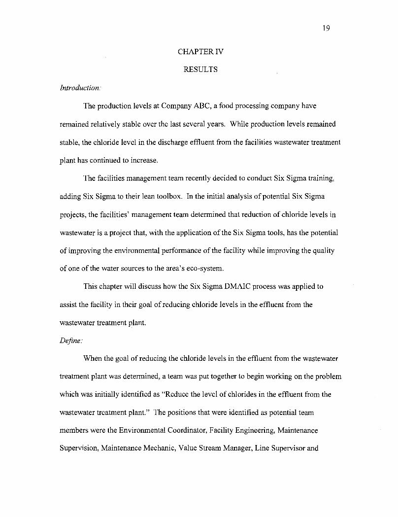
22
determine if any one, or any 01% type, of brine chiller was a major con.tributor to chloride
levels.
There are two types of brine chillers used in the facility. There are continuous
chills and batch chillers. The continuous chillers are part of an in-line processing system
that automatically moves the product h m the oven through the c h i l l i process. For the
batch chillers, the product must be physidly moved from the ovens to the chillers
allowing the product to be ohilfed.
Pareto Chart - Brine Chillers
................................... /--- I00 m o o - 70000 -
F 80 60000 - e ,o,o -_ _ _ _ _ _ _ _ _ _ _ _ _
a 60 E ? 40000 - - - - - - - -
E 30000 - 40 2
Chiller & d ecB & BF.' e6 &' gCB
Count 14658 14099 13215 12841 11912 9483 7260 1421 Percent 17.3 16.6 15.6 15.1 14.0 11.2 8.8 1.7 Cum% 17.3 33.9 49.4 M.6 78.6 89.8 88.3 100.0
Figure 3: Pareto Chart Brine Chillers
Analysis of the Pareto Chart for the Brine chillers (Figure 3) showed that the
chloride contribution h m the Ba*h Chillers was relatively consistent between identical
units. Brine Chillers 1 and 2, snd Brine Chillers 4 and 5 me identical units. Of the
identical units, chillers 1 and 5 showed &&ly lower chloride contribution. There is a
greater travel distance from the msns to chiller 1 than there is to chiller 2. There is also a

greater travel distance to chiller 5 than there is to chiller 4. The extra travel distance
results in a lower usage rate for chillers 1 and 5, offering a reasonable explanation for the
differences in their chloride contribution. Brine chiller 3 showed the largest single
contribution to chlorides. Brine chiller 3 is more centrally located in the facility and has
the highest utilization rate of the batch chillers. Brine chillers 7 and 8 are also identical
units. The analysis showed a significant difference between these two units, 7,260 lbs
per week and 13,215 lbs per week respectively. Brine chiller 6 showed the lowest
chloride contribution of any of the chillers. Brine chiller 6 is also used to chill a product
that is very different from the products that are chilled in the other systems.
After reviewing the data, the team determined that the first step would be to
reduce by 10% the level of chlorides contributed to the effluent from the wastewater
treatment plant from Brine Chillers 7 and 8. The second step would be to reduce the
level of chloride contribution from the batch chillers by 10%.
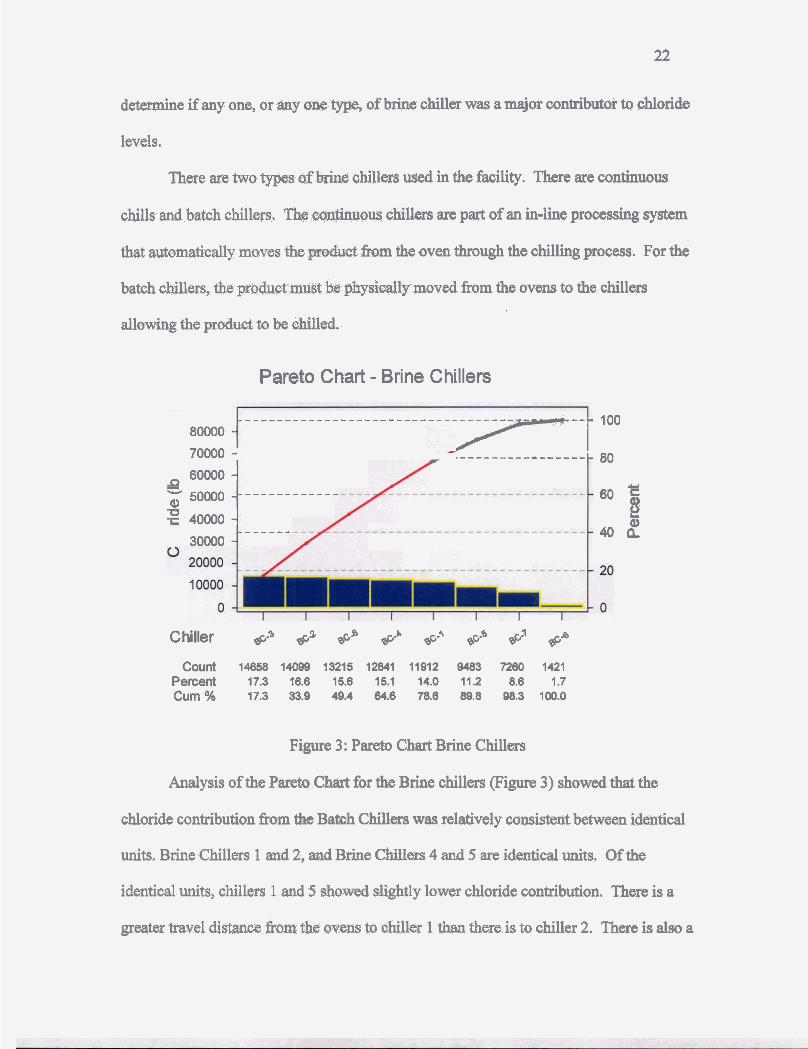
Measure:
In the define phase of the project, the team decided the key process output
variable was the chloride level in the wastewater effluent, measured in mg/l. The daily
chloride concentrations in the effluent from the wastewater treatment plant for the month
of January, 2006 are shown in Figure 4. The average chloride concentration for the
month was 2,248 mgll. The weekly average chloride concentrations for the fiscal year
2006 through January 2006 is shown in Figure 5. The average chloride concentration for
the fiscal year to date was 2,171 mgll.
January Chloride Concentrations
I I I
0 10 20
Sample Number
Figure 4: Daily Chlorides January, 2006
Weeky Average FY06 to January 31,2006
0 10 20 30 Week Number
Figure 5: Weekly Chloride Averages FY 06 to January 3 1,2006

In the measure phase of the project, the team needed to determine what key
process input variables would be measured. The first step in the process was to
determine the operating parameters for the brine chills as established by the facility's
Quality Control Department, shown in Table 1, below.
Brine Chill O~eration Parameters Chiller Lower Upper Target Temp Brine1
Specification Specification Concentration Water Limit (LSL) Limit (USL) Ratio
BC- 1 5 0% 65% 55% 16°F 60%/40%
Table 1 : Brine Chill Operation Parameters
Brine Chillers 1 through 5 are equipped with a PLC (Programmable Logic
Controller) that charges the chillers with a predetermined, metered mixture of saturated
brine and water to reach a brine concentration target. The BrineIWater Ratio
programmed in the PLC's results in a brine concentration that is above the target
concentration but within the Upper Specification Limit for the chillers.
The Brine Chillers 6 through 8 are equipped with older controls. Saturated brine
and water are added to the chiller by setting timers. Brine is metered, allowing the
facility to track the amount of brine used in each of the chillers. Brine concentration is
monitored on an hourly basis in the chillers. Based on the range of the brine
concentrations, from 45% to 75%, (see Figures 6 and 7), and the large difference in brine
usage between the two chillers 4,690 gallons of brine per week compared to 8,537

gallons per week, the team decided that the first step in the measurement phase would be
to determine if the brine metering systems were accurate.
To determine meter accuracy, a minute of brine was added to the brine reservoir
of each chiller, the brine meter totalizer reading was taken, the length and width of the
reservoir was measured, and the depth of the brine in the reservoir was measured to allow
the amount of brine in the reservoir to be determined and compared to the meter reading.
The testing revealed that incorrect parameters had been set up in the meters on Brine
Chiller 6 and Brine Chiller 8. The proper parameters were entered into the meter, and the
test was repeated. The meter parameters were then fine tuned until the totalizer reading
and volume of brine in the reservoir were within the accuracy tolerances specified by the
meter manufacturer. After the meter was corrected, brine use and concentration data
were collected for a month. The variation in brine concentration in the brine chillers did
not change. The average brine use in Brine Chiller 8 did decrease slightly while the brine
use in Brine Chiller 6 nearly doubled.
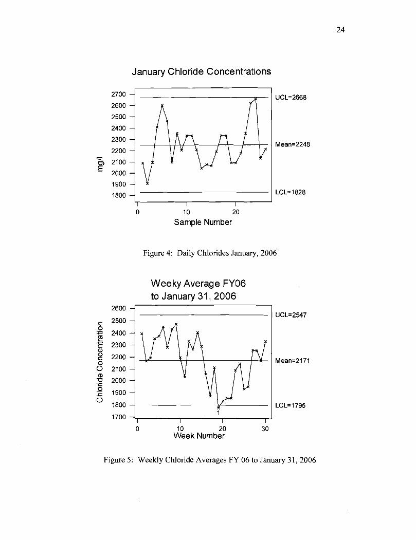
The hourly brine concentration readings from Brine Chillers 7 and 8, for the
month of January, 2006, were placed on run charts (Figure 6 and 7). The run charts
show that the brine concentrations ranged from the lower specification limit of 45% to
75%, which is above the upper specification limit of 65%. The lower control limit was
calculated as 50.15% while the upper control limit was calculated as 64.24%. The run
charts clearly show that the process of maintaining brine strength in Brine Chillers 7 and
8 is out of control.
Brine Chiller 7 Run Chart January, 2006
I I I I 0 100 200 300
Sample Number
Figure 6: Run Chart for Brine Chiller 7, January, 2006
Brine Chiller 8 Run Chart January, 2006
I I
I I I
0 100 200 300
Sample Number
Figure 7: Run Chart for Brine Chiller 8, January, 2006

Analyze:
The first step in the analyze phase of the project was to determine the process
capability of the two Brine Chillers (Figure 8 and 9). The range between the lower and
upper specification F i t s for brine strength is 15%. The range between the lowest and
highest measured brine concentration was 33%. The process capability analysis
projected that the salt concentration in Brine Chiller 7 would be below the lower
specification limit (LSL) or above the upper specification limit (USL) approximately
28% of the time. In comparison, the process capability analysis projected that the salt
concentration in Brine Chiller 8 would be outside of the specification limits
approximately 39% of the time.
Process Capability Analysis for January Brine Chiller 7
Pmcess Data USL 60.0000 Target LSL 45.0000 Mean 54.7756 Sample N 254 StDev nn/ithin)2.09576 StOev (Overa14.49697
1 I
Overall
I I Potential Within) Capability I I
CP 1.19 CPU 0.83
I CPL 155 ------ CPk 0.83 I I I I I
Overall Cnpabilny Oblerded Perfoman~e Exp. 'Withid' Performance Exp. "Overall' Perfonanc
PP 0.38 PPM cLSL 0.00 PPM c LSL 1 55 PPM c LSL 66208.59 PPU 0.27 PPM > USL 173228.35 PPM USL 6336.16 PPM > USL 210660.98 PPL 0.50 PPM Total 173228.35 PPM Total 6337.71 PPM Total 278869.57 PPk 0.27
Figure 8: Brine Chiller 7, January, 2006 Process Capability

Process Capability Analpis for January Brine Chiller 8
PK%eaa Dsia LSL USL
USL 60.0000
'"" LSL 45.0,; Mean 57.1830 Sample N 316 StDev (WitMn)237SW
Potential Wlhin) Capablllty I CP 1.05 I CPU 0.39 CPL 1.71 ---*--
Ovmll Capapabilky ObPwed Peifwmawe Exp. Wlthin" P e d o f m m EX~. 'Wudr Perlomare Pp 0.35 PPMeLSL 0.00 PPM < LSL 0.16 PPM<LSL 453M11 W U 0.13 PPM>USL 587974.68 PPM>USL 119113.65 PPM>USL 9.18875.09 W L 0.57 WMTcW 287974.88 PPMTotd H9 l lb80 PPMTotsl 3EW4S.30 Ppk 0.13
Figure 9: Brine Chiller 8, January, 2006 Process Capability
The second step in the analyze phase was to conduct a problem solving meeting
with the process owners to determine why there was such a large range in the brine
concentration on a day-to-day and how-to-how basis. After reviewing the January run
charts (Figures 6 and 7) and the process capability analysis (Figures 8 and 9), decided on
a current performance statemat of "Chloride usage in the Brine Chillers 7 and 8 is out of
control" with a goal of "Reduce chloride usage in Bnhe Chillers 7 and 8 by 10% by
March 3 1,2006." The cause and effect analysis from the problem solving meeting is
shown in Figure 10. The team then conducted a root cause analysis
Measurement F Goal will be measured
againse current performance of -2,200
mg/l of Chlor~des in Wastewater
Chlorides in Wastewater Stream from -2,200 to 1.800
Environment
Not trained in Correct Method of add~ng Raw
Brine, Brine Addltion is not based on Calculations
Too Much Chloride is
added
Brlne is Added based on Experience of
Smokemaster Need Beter Method to Keep
Control Usage in the Brine Chillers
Not Capable of Addng Brine by the Gallon, only by
the Minute
Figure 10: Problem Solving Cause and Effect Diagram
using the 5 Whys approach. The questions and answers that were developed in the
exercise were:
1. Why is chloride usage so high? Brine addition is based on experience, not on the
brine strength readings. Some Smokemasters (Operators) are trained in reading
the salometer. The system is not capable of adding saturated brine by the gallon,
only by minutes of flow. The salometer, brine concentration target is too high.
2. Why is brine add-back based on experience? There is no standardized work or
guidance to help the operators determine how much brine to add back to the
system to maintain brine concentration. Brine is added to the system based on
minutes of flow, not gallons.
3. Why is there no standardized work for adding brine? Standardized work has
never been an issue in the area.
4. Why is it that the chillers cannot add brine by the gallon? The controllers are not
set up for addition by the gallon, only with timers.

5. Why do the operators target a high salometer of 68 to 72% if the target is 50%? It
is easier for the operators as they do not have to add brine to the system as often
when they add back to a higher brine concentration.
6. Why do operators not know how to read a salometer correctly? There is no
standardized work for the operators.
7. Why are the brine meters not accurate? The proper correction factors were not set
up in the meters when they were installed.
8. Would lowering the brine concentration to the target work? Would lowering the
brine concentration result in lower brine usage and lower chloride levels? Yes.
The problem solving group several steps that needed to be completed to address the root
causes that were identified. The steps included establishing a standardized work guide
for the operators to follow when adding brine back to the chillers, standardized work for
taking and reading the salometer, and reprogramming of the PLC to allow saturated brine
to be added to the chillers based on gallons for flow rather than minutes of flow..
A similar procedure was followed to analyze the brine usage in the batch chillers.
The team found that the lower specification limit for the brine chillers 1 through 5 was
higher than for brine chillers 6 through 8, the target temperature of the brine was 10 to 12
degrees lower for the brine chillers 1 through 5 than for the brine chillers 6 through 8, and
that the brine addition to the chillers was controlled by the PLC, charging the chillers and
adding brine back into the chillers with a concentration that is higher than the target. The
Quality Control department was able to determine that there was no logical reason for the
differences in the specifications for the Batch Chillers and agreed to modify the
specifications so that all of the batch chillers are the same.

Implement:
The first step in the implementation process was to develop a brine addition and
waste schedule for the brine chiller operation while also developing standardized work
for the operation of the Brine Chillers. A chart and instructions on how much brine to
add back to and dump from the chillers to maintain the proper salt concentration and
brine level was prepared for the operators during the same time frame as the operating
instruction sheet for checking brine concentration was developed (Figure 11). An
operating instruction form (standardized work) was developed that was used to train the
operators on the proper method of determining the brine concentration. The operating
instruction form was also posted in the work areas allowing the operators to utilize the
form as a check list when performing the task. The operating instruction form is shown
on the next page, Figure 12. The form is based on the recommendations from the Salt
Users Guide, published by International Salt in 1992.
Brine Addition
Figure 1 1 : Brine Addition Chart
Figure 12: Standardized Work to C
heck Salt Concentration

The PLC program for the batch brine chillers was modified to vary the brine
concentration based on the required brine temperature. When the brine temperature is
required to be at or less than ~o'F, the brine will be loaded and added to the chillers at a
55% concentration. When the required brine temperature is above 20°F, the brine will be
loaded and added to the chillers at a 50% concentration. The updated specification table
is shown in Table 2 on the next page.
Brine Chill O~eration Parameters (Revised) Chiller
BC- 1
Lower Upper Target Temp Brine / Specification Specification Concentration Water Limit (LSL) Limit (USL) Ratio
45% 60% 5 0% +20 '~ 50%/50%
BC-8 45% 60% 50% 2 6 ' ~ Table 2: Revised Brine Chill Operation Parameters
Control:
Controls must be implemented to ensure that over time the brine use in the
chillers does not return to previous levels. The following actions were taken to ensure
that any reductions in brine use and chloride concentrations continue into the future:
The use of the operating instruction form (Figure 1 1).
The brine addition chart (Figure 12).

The revised Brine Chill Operation Parameters (Table 2).
The temperature set point and brine mixing formula in the PLC's on the
batch brine chillers was password protected, requiring an Electronic
Technician or Value Stream Manager to change set points.
Steps were added to the job plan in the Computerized Maintenance
Management System (CMMS) requiring a qualified Electronic
Technician to install/replace/repair flow meters to ensure that the proper
correction factors are programmed into the meter when installed.

CHAPTER 5
DISCUSSIONS
Summary of Results:
The brine addition chart went through several revisions. The initial revisions
were designed to make the instructions more user friendly for the operators. The
salometer is designed and calibrated to accurately measure the brine concentration when
the brine temperature is 60'~. The operating temperature of the brine in the facility's
chillers ranged from 1 6 ' ~ to 25'~. The correction factor for the salometer is to adjust the
reading by 1% for each 1 O'F difference between the brine temperature and the calibration
temperature of the salometer (International Salt, 1992). For example, if the salometer
reading is 52% and the brine temperature is 24'~, the actual corrected salometer is (52-
((60-24)/10, or 48.6%. The brine addition chart was adjusted so that the recommended
volume of brine to add back to the system was based on the setpoint temperature for the
brine, eliminating the need for the operators to calculate the actual brine concentration.
The initial requirement of draining some brine off the system prior to adding fresh
brine was eliminated. The Process Owners initially believed that adding brine without
draining would result in an overflow condition in the brine chillers. The team found that
the brine level dropped to the point that excessive amounts of saturated brine needed to
be added to the system to maintain the minimum operating level when a drain step
occurred. There was enough brine being carried out of the system on the product, that
simply adding brine to maintain concentration resulted in a stable brine level in the
chiller.

As control of the brine concentration improved, and the risk of freezing the heat '
exchangers lowered, the brine addition chart was adjusted downward to move the average
brine concentration to the lower end of the operating range to reduce brine usage which
was expected to assist in reducing chloride levels in the wastewater effluent. The current
version of the Brine Addition table is designed to allow the operators to control the brine
concentration between 45% and 50% (Figure 13). Brine concentration is checked hourly
in the continuous chillers. Figure 14 shows the hourly brine concentrations since January
1,2006 in Brine Chiller 7 while Figure 15 shows the same information for Brine Chiller
8. The initial testing was done with Brine Chiller 7. The testing started in the area of
sample 300 where an initial downward shift of the brine concentration can be seen. At
approximately sample 600, the brine concentration was adjusted downward and the
operators were instructed to charge the chiller with 500 gallons of saturated brine at the
Monday morning start up. Minor adjustments were made to lower brine concentration
after sample 750. The year to date brine concentration in chiller 7 was lowered from
54.78% to 5 1.10%, a reduction of 6.72%. Since the most recent change in the brine
addition schedule, the brine concentration has averaged 47.1 1% (Figure 16), a reduction
of 14.00%.
When the team was comfortable with results from Brine Chiller 7, the
standardized work and brine addition schedule was implemented on Brine Chiller 8,
approximately at sample 600. After sample 600, as minor adjustments were made to
Brine Chiller 7, they were implemented on Brine Chiller 8. On a year to date basis, the
average brine strength in Brine Chiller 8 has been reduced from 57.19% to 5 1.82%, a
reduction of 9.39%. Since the most recent change in the brine addition schedule, the

3 8
brine concentration has averaged 47.09% in Brine Chiller 8 (Figure 17), an overall
reduction of 17.66%. The run chart does show that the brine concentration started to
trend downward before any changes were implemented. The team attributes the
downward trend to the increased attention that was directed at the operation of the two
chillers. Both chillers are under the control of the same operator.
Brine Addition
Monday Startup: T h e initial brine charge, on startup on Monday mornings, to achieve 50'5 target i s 5 0 0 gallons and -4.5 minutes o f water
Daily Startup Afer CI P At start u p during the week, check the brine salometer after it h a s been returned to the brine sump and cllillecl to o l )e~a t i~ lg telnl)elatule. A d d brine to the sump based on the chart above. I f the salometer i s 5 0 ' s o r hiaher. do not add brine.
Normal Operation (Hourly): During normal operation, find the salometer reading in in the chart above. Go over to the next column on the right and add the gallons o f brine indicated.
Do not Dump Brine from the System.
Figure 13 : Current Brine Addition Schedule

Run Chart Brine Chiller 7 YTD
0 1000 2000 Sample Number
Figure 14: Brine Chiller 7 Run Chart Year to Date
Run Chart For Brine Chiller 8 YTD
I I I 0 1000 2000
Sample Number
Figure 15: Brine Chiller 8 Run Chart Year to Date

Run Chart Brine Chiller 7 May 2006
54 -
I I I I I
0 100 200 300 400
Sample Number
Figure 16: Brine Chiller 7 - Current Run Chart
Run Chart Brine Chiller 8 May 06
54 -
I I I I I I I I
0 100 200 300 400 500 600 700
Sample Number
Figure 17: Brine Chill 8 Most Recent Run Chart

The capability of the process to maimin brine concentration has improved as
shown by comparing Figures 8 and 9 with Figures 18 and 19 or by reviewing Table 3.
Table 3: P w s Capability Comparisons
Pmess Data USL 80 WOO Tarsst LSL 45.WOO Maan 47.1063 Sample N 349 Stow (Wnhin)l.32525 SDsv (Overdr).75242
Potential (Within) CspMBy
CP 1.89 CPU 3.24 CPL 0.53
CPk 0.53
Process Capability Analysis Brine Chiller 7 - May 06
Overall Capsbilly Observd Psrfonnanee Exp. Wkhln" Pwlormame Exp. "Ovusll" Ps*ormme PP 1.45 PPM < LSL 22922.64 PPM C LSL 55988.90 PPM e LSL 114693.50 PPU 2.45 PPMs USL 0.00 PPMz USL 0.00 PPM, USL 0.00 PPL 0.40 PPM Total 22922.84 PPM Total 55988.W PPM Told 114693.50 Ppk 0.40 .
Figure 18: Current Process Capability Brine Chiller 7

Process Capability Malysts Brine Chiller 7 May 06
PWS Data USL BO.OOW Tarsot LSL 46.OMX1 Wan 47.0991 sample N 549 StDw wihin)1.29191 StDw (Ove~4U.65756
Potential (Wnhln) Capability
CP 1.91 CPU 3.33 CPL 0.54
Ovemll Cspbilny Obsewed Perronancs Exp. WdNn' Pufmsnce Exp. 'Ovemll" Pmfonnsno PP 1.61 PPM U LBL 14328 65 PPM < LSL 52103.08 PPM < LSL 8887S.23 PPU 2.76 PPM* USL 0.00 PPM> USL 0.00 PPM >USL 0.00 PPL 045 PPMmtsl 14SS66 PPMTMd 52103.09 PPh4Tot.l 88875.23
PPk 0.46
Figure 19: Cment Process Capability Brine Chiller 7
The process capability studies on the chillers show that while that risk of
operating above the upper specification limit has been virtually eliminated, the risk of
operating below the lower specification limit has greatly increased The risk of freezing
the heat exchangers is relatively low until the brine concentration drops below 41%. The
chiller operators have been given the discretion to allow the brine strength to drop below
the lower specification limit (45%) at the end of the production run to reduce brine waste.
The expectation of in-specification performance has been increased from 72.3% to 88.5%
while reducing the brine concentration by 14.00% in Brine Chiller 7. In Brine Chiller 8
the expectation of in specification performance has been increased from 61% to 91.1%
while reducing the brine c o n c e ~ ~ by 17.6%.
The purpose of the project was to determine if utilization of the Six S i
methodology could reduce the chloride concentration in the effluent from the facility's

wastewater treatment plant. In the month prior to the start of the project the chloride
average weekly chloride concentration in the effluent was 2,248 mgll (Figure 4) while the
fiscal year to date (July, 2005 through January, 2006) weekly average was 2,171 mg/l
(Figure 5). In comparison, in May of 2006, the average chloride concentration was 1,615
mg/l (Figure 20) while the fiscal year to date average chloride concentration had dropped
to 1,980 mgll (Figure 2 1). The average weekly concentration during the month of May
Chloride Concentration May, 2006
I I I I 1 2 3 4
Sample Number
Figure20: Chloride Concentration May, 2006
was 25.6% below the year to date weekly average at the end of January and 18.4% below
the year to date average.

Cliloride Concentration January to May 2006
2500 -
Sample Number
Figure 2 1 : Chloride Concentration January to May 2006
Utilizing the Six Sigma methodology to analyze the sources of chlorides in the
effluent from the wastewater treatment plant, then following the sources upstream, and
using the Six Sigma tools to define, measure, analyze, improve and control the operation,
has had a significant effect on the facility's efforts to reduce the chloride concentration.
As a result of this study, formal guidelines have been established for the operation of the
continuous brine chilling systems, rather than allowing the systems to be operated solely
by operator experience.
Future Research:
The Relationship Between Brine Temperature and Chill Rate:
The mindset in the facility, and in the industry, is that colder is better. Several of
the brine chill operators mentioned that the product often reaches a given temperature and
stays at that temperature until the product is pulled from the brine chiller and allowed to

temper in a holding cooler. In several chillers the set-point for the brine temperature was
1 R OF, which is well below the freezing point of the product. The product may be crust
frozen, sealing the heat inside the product. Further studies should be done to determine
the relationship between brine temperature and the rate of product cooling. The facility
may find that by allowing the brine temperature to rise, the product may cool more
quickly. A warmer brine temperature will allow the facility to use a lower concentration
of brine, further reducing chloride use.
Brine Pressure and Chill Rate:
The Brine Chillers 6, 7, and 8 utilize a deluge system to chill the product. The
cold brine is fed into perforated trays that mimic a cold shower over the product. The
other Brine chillers have a pressure pump that discharges the brine through spray nozzles
to create a distribution patter. The operators have noticed that there appears to be more
brine loss from the tracks in the newer chillers that operate at a higher pressure. Further
testing should be done to determine if the product can be cooled just as quickly with a
lower pressure spray
Extension of Brine Life:
Brine is re-utilized in the three of the brine chillers for up to a week.
Consideration should be given to implementing similar brine reuse programs in the other
chillers to reduce chloride use.
Ultra-filtration equipment is available on the market that is capable of removing
bacteria from liquids. With further testing, the facility may be able to extend brine life
beyond a week using a combination of ultra-filtration, pasteurization, and rechilling of
brine.

Other Sources:
Water softeners accounted for approximately 6.6% of the chlorides in the
wastewater effluent. The current method of water softening needs to be investigated. It
may be possible to reduce the salt use in the water softeners by as much as 50% if the
resin bed can be fluffed with air injection, similar to the method that is used in the
regeneration of the resin beds for corn syrup and salt brine purification system.

Reference List:
Bothe, D., (2003) Accelerated Six Sigma Green Belt Certzjicate Program.
Cedarburg, WI: International Quality Institute, Inc.
Breyfogle 111, Forrest, (2003). Implementing Six Sigma, Hoboken, NJ: John Wiley
& Sons, Inc.
Brue, G., (2002). Six Sigma for Managers, New York, NY: McGraw-Hill Companies,
Inc.
DiGiano, F., Elais, M., Francisco, M., LaRocca, C., Maerker, M. Report 276:
Chronic Toxicity Bioassay with Ceridaphnia dubia: (n.d.) Retrieved
April 8,2006 from http://www2.ncsu.edu/scsu/~~~i/reports/cisco.html
Eckes, G., (2003). Six Sigma for Everyone. Hoboken, NJ: John Wiley & Sons, Inc.
Emiliani, Bob, (2003) Better Thinking, Better Results, Kensington, Ct: The Center for
Lean Business Management LLC
General Electric (2001) Six Sigma at GE 2001. Retrieved April 8,2006
From http://www.gehealthcare.com/twzh/sourcing/data/6S.ppt
General Electric, (n.d). What Is Six Sigma? The Roadmap to Customer Impact
Retrieved February 25,2006 from
http://www.gepowercontrols.com/ex/news~events/six - sigma.htm
George, Michael L. (2002) Lean Six Sigma, Combining Six Sigma Quality with Lean
Speed New York: McGraw-Hill
Gupta, P., (2004). Six Sigma Business Scorecard, New York, NY: McGraw-Hill Companies, Inc.
Larson, A., (2003). Demystzjjing Six Sigma, New York, NY: American Management
Association

Mack, Lindsey, Food Preservation in the Roman Empire Retrieved February 24, 2006,
from http://www.unc.edulcourses/rometech~public/contents/swival
/Lindsay-MacWFood-Preservation.htm
United States Environmental Protection Agency, (January 2002). Development
Document for the Proposed Efluent Limitations Guidelines and
Standards for the Meat and Poultry Products Industry Point Source Category (40
CFR 423), EPA-821 -B-01-007
United Stated Environmental Protection Agency, Environmental Monitoring
Systems Laboratory, (1 994) Short-Term Methodsfor Estimating the
Chronic Toxicity ofEffluents and Receiving Waters to Freshwater Organism.
EPA/600/4-921002. Retrieved April 8,2006 from http://epa.gov
Wisconsin Department of Natural Resources, (n.d.) Chapter 1.3 - Representative Data,
Reasonable Potential & WET Monitoring, Retrieved on February 7,2006 from
http://dm.stat.wi.gov/org/water/wm/w/bi~mon~docs/cap 1 X3MonitoringLimits.
Wisconsin Department of Natural Resources, (2000) Chapter 2.10 - Chlorides
and WET Testing, (2000). Retrieved on February 7,2006 from
http://dm.stat.wi.gov/org/water/dww/biomon.docs/cap2X1 Ochloridewed.
Wisconsin Department of Natural Resources, (n.d.) Chloride Variance
Information and Worhheet, Retrieved on February 7,2006 from
http://dm.stat.wi.gov/org/water/wm/w/applications/chloride~wksht.pdf