Real-Time Graphics Processing Unit Implementation of Whitening Filters for Audio Signals
by Omer A.S. Osman
B.S. in Electrical Engineering, May 2010, The George Washington University
A Thesis submitted to
The Faculty of The School of Engineering and Applied Science
of The George Washington University in partial satisfaction of the requirements
for the degree of Master of Science
August 31, 2011
Thesis directed by
Miloš Doroslovački Associate Professor of Engineering and Applied Science

ii
© Copyright 2011 by Omer A.S. Osman
All Rights Reserved.
iii
Abstract
Real-Time Graphics Processing Unit Implementation
of Whitening Filters for Audio Signals
This work investigates a real-time implementation of autoregressive and
pitch-prediction whitening filters for use in audio feedback suppression. The work begins
by analyzing whitening filters performance for synthesized and recorded test audio
signals. A MATLAB simulation of the adaptive feedback cancellation (AFC) algorithm
shows pitch-prediction to be the most computationally intensive aspect of the feedback
cancellation algorithm. A DSP processor implementation is demonstrated in which the
autoregressive filter implementation outperforms MATLAB implementation computation
time while the pitch-prediction implementation fails to meet real-time requirements. A
successful real-time implementation of the pitch-prediction algorithm is demonstrated on
NVIDIA graphics processing unit (GPU) with substantial speed gains compared to the
MATLAB implementation.
iv
Table of Contents
Abstract ............................................................................................................................... iii
Table of Contents ............................................................................................................. iv
List of Figures ................................................................................................................... vii
List of Tables ................................................................................................................... viii
Glossary of Terms and Acronyms ............................................................................... ix
Chapter 1 – Introduction ................................................................................................ 1
1.1. Research Problem ............................................................................................................. 1
1.2. Autoregressive Modeling ................................................................................................ 3
1.3. Pitch Linear Prediction Modeling ................................................................................ 3
1.4. Contributions ...................................................................................................................... 4
Chapter 2 – Theoretical Background ......................................................................... 5
2.1. Autoregressive Modeling using the Autocorrelation Method ............................ 5
2.2. 3-‐Tap Pitch Prediction Model ........................................................................................ 6
2.3. Issues in Real-‐Time Implementation .......................................................................... 8
Chapter 3 – Autoregressive and Pitch Prediction Filters Performance ......... 9
3.1. Test Filters Conditions ................................................................................................... 10
3.2. Test Metrics ....................................................................................................................... 11
3.3. Synthesized Test Signals ............................................................................................... 13
3.3.1. Colored Noise ............................................................................................................................. 13
3.3.1.1. Autoregressive Filter Response to Synthesized Colored Noise ................................... 15
3.3.2. Synthesized Ab Note ................................................................................................................ 18
3.3.2.1. Cascade Filter Response ............................................................................................................... 19
v
3.4. Recorded Test Signals .................................................................................................... 20
3.4.1. Recorded Speech Signals ...................................................................................................... 21
3.4.1.1. Speech Sibilance Signal ................................................................................................................. 21
3.4.1.1.1. Autoregressive Filter Response to Recorded ‘s’ Sound ......................................... 22
3.4.1.2. Speech Vowel Signal ....................................................................................................................... 24
3.4.1.2.1. Autoregressive Filter Response to Recorded ‘ah’ Sound ...................................... 25
3.4.2. Recorded Musical Notes ........................................................................................................ 29
3.4.2.1. Monophonic Audio Signal -‐ Piano Note .................................................................................. 29
3.4.2.1.1. Cascade Pitch and Autoregressive Response – Monophonic Input Signal .... 30
3.4.2.2. Polyphonic Audio Signal – Piano Chord ................................................................................. 33
3.4.2.2.1. Cascade Pitch and Autoregressive Filters Response – Polyphonic Input ...... 34
3.4.2.3. Polyphonic Audio Signal – Piano Chord with Bass Note ................................................. 35
3.4.2.3.1. Cascade Pitch and Autoregressive Filters – Polyphonic Input with Bass Note
.................................................................................................................................................................................... 36
3.5. Discussion .......................................................................................................................... 38
Chapter 4 – DSP Implementation .............................................................................. 40
4.1. Challenges in Implementation .................................................................................... 40
4.2. Target Architecture ........................................................................................................ 41
4.3. DSP Processor vs FPGA .................................................................................................. 41
4.4. DSP Processor Performance Results ........................................................................ 42
4.4.1. Recorded Sibilance – AR Filter Testing .......................................................................... 42
4.4.2. Recorded Ab Piano Note ........................................................................................................ 44
4.4.3. Processor Profiling .................................................................................................................. 44
4.5. Problems Encountered .................................................................................................. 46
4.5.1. Memory Segmentation ........................................................................................................... 46
4.5.2. Stack Overflow .......................................................................................................................... 46
vi
4.5.3. Hardware Division ................................................................................................................... 47
4.6. Discussion .......................................................................................................................... 47
Chapter 5 – GPU Implementation .............................................................................. 48
5.1. Target Architecture ........................................................................................................ 48
5.2. Algorithm Implementation .......................................................................................... 49
5.2.1. PLP Filter Implementation ................................................................................................... 49
5.2.2. AR Filter Implementation ..................................................................................................... 51
5.3. Numerical Accuracy in CUDA Implementation ...................................................... 52
5.4. Problems Encountered .................................................................................................. 53
Chapter 6 -‐ Conclusions ................................................................................................ 55
6.1. Filters Performance ........................................................................................................ 55
6.2. Development Cost ........................................................................................................... 56
6.3. Final Remarks ................................................................................................................... 56
References ......................................................................................................................... 57
Appendix A – DSP Implementation Code Listing .................................................. 59
Appendix B – GPU Implementation Code Listing ................................................. 74
Header File with Algorithm Definitions ........................................................................... 74
Main Driver File ....................................................................................................................... 74
CUDA GPU Driver File ............................................................................................................. 85
vii
List of Figures
Figure 1-‐1 MATLAB Profiling of AFC Algorithm Showing Linear Prediction Time Consumption __________ 2
Figure 3-‐1 Colored Noise Source using a Butterworth Filter fc = 3 kHz ___________________________________ 14
Figure 3-‐2 Frequency Response of the AR Filter with Colored Noise Input ________________________________ 15
Figure 3-‐3 Pole-‐Zero Plot Demonstrating AR Filter Response _____________________________________________ 16
Figure 3-‐4 AR Filter Residual Signal Showing a Flattened Spectrum _____________________________________ 17
Figure 3-‐5 Synthesized Ab Note Frequency Spectrum ______________________________________________________ 18
Figure 3-‐6 Residual Spectrum after Cascaded PLP and AR Filters Whitening ____________________________ 20
Figure 3-‐7 Recorded 's' Sound from a Male Voice __________________________________________________________ 22
Figure 3-‐8 Whitened Recorded 's' Signal Filtered using Autoregressive Filter ___________________________ 24
Figure 3-‐9 Recorded 'ah' Sound from a Male Voice Input Signal Spectrum _______________________________ 25
Figure 3-‐10 Cascade PLP and Autoregressive Filters Structure ___________________________________________ 25
Figure 3-‐11 Cascade Filter Structure with Pre-‐Whitening Filter __________________________________________ 26
Figure 3-‐12 Residual Spectrum of ‘ah’ Vocalization after AR Filtering ___________________________________ 27
Figure 3-‐13 Residual Spectrum of Cascade Filters of Recorded 'ah' Sound _______________________________ 28
Figure 3-‐14 Recorded Ab Piano Note ________________________________________________________________________ 30
Figure 3-‐15 Cascade PLP Filter Output Residual with Pre-‐Whitening ____________________________________ 32
Figure 3-‐16 Polyphonic Test Signal with an Ab7 Piano Chord ______________________________________________ 33
Figure 3-‐17 Cascade PLP and AR Filters Residual for Ab7 Chord Polyphonic Input ______________________ 35
Figure 3-‐18 Recorded Ab7 Chord with Ab Bass Note _______________________________________________________ 36
Figure 3-‐19 Residual of Cascade PLP and AR Filter for Polyphonic Input with Bass Note _______________ 38
Figure 5-‐1 Comparison of Cascade Residual Spectrum using MATLAB and CUDA _______________________ 53
viii
List of Tables
Table 3-‐1 Autoregressive Filter Response to Colored Noise ________________________________________________ 17
Table 3-‐2 Signal Whitening of Synthesized Ab Note using PLP and Cascade PLP – AR Structure ________ 19
Table 3-‐3 Autoregressive Filter Response to Recorded Sibilance __________________________________________ 23
Table 3-‐4 Recorded 'Ah' Sound Cascade Filters Residual __________________________________________________ 26
Table 3-‐5 Cascaded PLP and AR Filter Residual with and without Pre-‐Whitening _______________________ 31
Table 3-‐6 Polyphonic Signal Filtering _______________________________________________________________________ 34
Table 3-‐7 Cascade Filters Response to Polyphonic Input Signal with Bass Note __________________________ 37
Table 4-‐1 Simulation Results Comparison for the Autoregressive Filter Residual ________________________ 43
Table 4-‐2 Residual Spectrum Kurtosis for the DSP Implementation of the 3-‐Tap PLP Filter ____________ 44
Table 4-‐3 DSP Processor Profiling Results Comparison ____________________________________________________ 45
Table 5-‐1 GPU Implementation of PLP Processing Time ___________________________________________________ 50
Table 5-‐2 Comparison of Signal Whitening using MATLAB and CUDA ____________________________________ 52
ix
Glossary of Terms and Acronyms
Autoregressive model (AR) – an all-pole model for random processes
Compute Unified Device Architecture (CUDA) – parallel computing architecture
developed by Nvidia. Basis of the architecture of the GPU used in this work
Graphics Processing Unit (GPU) – specialized processor for high-speed image
processing with emerging general-purpose uses that exploit its parallel architecture
MATLAB – numerical computing software package used to develop and verify
algorithms
Monophonic signal – signal with a single fundamental frequency
Pitch Linear Prediction (PLP, 1T PLP, 3Ts PLP) – a form of modeling that depends
on harmonic frequencies in the modeled spectrum. Used in this work for either one-
tap or 3-tap modeling based on suboptimal search.
Polyphonic signal – signal with multiple fundamental frequencies (e.g. piano chord)
Sibilance – unvoiced speech similar to producing the letter ‘s’
Whitening – process of filtering to produce a flattened spectrum (spectrum that is
similar to white noise)
1
Chapter 1 – Introduction
Linear prediction is a technique of mathematical modeling of dynamic time
varying systems. It has wide applications including neurophysics (modeling of brain
activity) [1], geophysics (analysis of seismic traces for oil exploration) [2], and in
speech applications (speech coding and audio compression) [3]. The strength of the
technique lies in its simplicity under wide range of situations. The focus of this work
is in the real-time application of two variants of linear prediction in an audio
application.
1.1. Research Problem
The motivation for this work comes from current research in acoustic feedback
cancellation (AFC) [4]. A recent survey of adaptive acoustic feedback suppression
techniques from the past fifty years has found that acoustic feedback cancellation
(AFC) produced the most promising results, in terms of maximum stable gain and
sound quality, for both hearing aid and sound reinforcement systems [5]. The greatest
challenge in AFC is in reducing the computational complexity, inherent in the use of
high sampling rate in audio applications [5]. This work aims to tackle the most
computational intensive aspect of the real-time implementation of the AFC algorithm.
Linear prediction models are used in closed loop decorrelation of the audio signal
in the AFC algorithm [4]. Comparison of AFC performance with various
decorrelation techniques has found that the use of decorrelating (whitening) pre-filters
to be the preferred method from both sound quality and maximum stable gain points
2
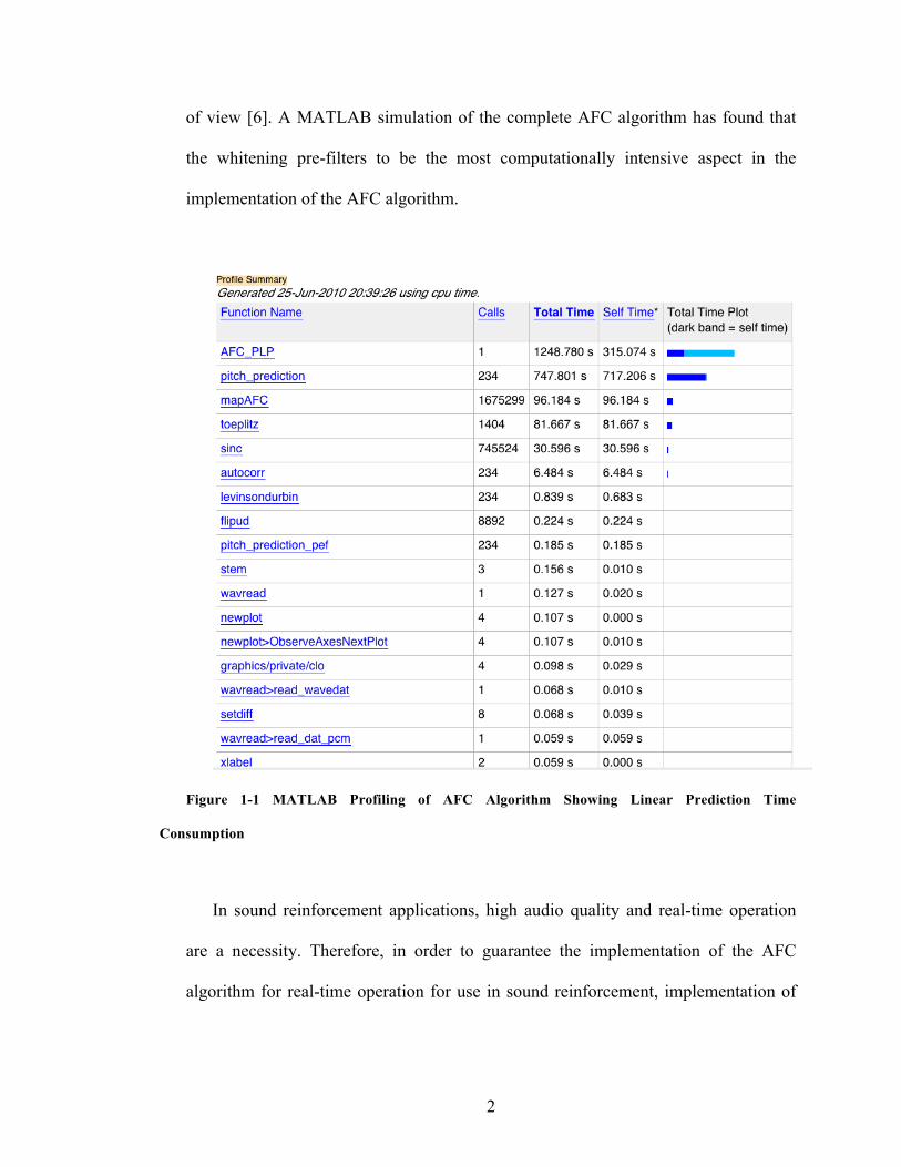
of view [6]. A MATLAB simulation of the complete AFC algorithm has found that
the whitening pre-filters to be the most computationally intensive aspect in the
implementation of the AFC algorithm.
Figure 1-1 MATLAB Profiling of AFC Algorithm Showing Linear Prediction Time
Consumption
In sound reinforcement applications, high audio quality and real-time operation
are a necessity. Therefore, in order to guarantee the implementation of the AFC
algorithm for real-time operation for use in sound reinforcement, implementation of
3
the whitening pre-filters in real-time must be resolved first before the other
components of the AFC algorithm. This is the focus of this work.
1.2. Autoregressive Modeling
The whitening pre-filters, used in the AFC algorithm, are represented by a
cascade autoregressive filter (AR) and pitch linear prediction filter (PLP). In the
figure above, the computation time for the pitch linear prediction filter is under
‘pitch_prediction’ while the autoregressive filter is shown under ‘autocorr’ and
‘levinsondurbin’. Although the autoregressive filter is not the most time consuming, it
is implemented in this work due to its close relationship to the pitch prediction filter.
More generally, autoregressive modeling is the simpler of the two techniques
discussed in this work. Autoregressive modeling has wide use in speech coding [3,7].
Two methods are used in generating the filter coefficients. The autocorrelation
method will be used in this work due to its guaranteed stability [7].
1.3. Pitch Linear Prediction Modeling
The PLP filter also has wide use in speech coding applications [8]. The PLP filter
is used to model quasi-periodicity of the tonal component of speech or audio signals.
The filter is used in the cascade AR – PLP or PLP – AR structure, to remove quasi-
periodicity of the tonal component of the signal and enhance the overall whitening of
the residual spectrum.
4
1.4. Contributions
This work discusses the implementation of the autoregressive and pitch linear
prediction filters for audio signals for application in acoustic feedback cancellation.
The goal of this work is to present a practical implementation of the filters and to
present the applicability of these filters to real audio signals. In Chapter 2, a brief
summary of the theoretical background relating to the two filters is discussed. In
Chapter 3, three test metrics are presented, which are used to analyze the performance
of the filters against synthesized and recorded samples of speech and audio signals.
Two of both filters are discussed in detail. In Chapter 4, a DSP processor
implementation is discussed. The applicability of DSP processor architecture for this
algorithm is discussed. Performance results are demonstrated and discussed.
In Chapter 5, a massively parallel implementation on NVIDIA graphics
processing units (GPU) is discussed. This implementation exploits parallelization
inherent in the PLP algorithm. Performance gains are demonstrated by exploiting
parallelization in the PLP algorithm.
In Chapter 6, a concluding discussion is conveyed which discusses the
significance of the performance gains achieved in the massively parallel
implementation. This chapter concludes with a brief discussion of the complete
implementation of the AFC algorithm and points for further research.
5
Chapter 2 – Theoretical Background
Both autoregressive (AR) and pitch linear prediction (PLP) modeling have had
early success in speech applications. In this section, published literature detailing the
two methods are summarized. This chapter concludes with considerations involving
real-time operation of the filters.
2.1. Autoregressive Modeling using the Autocorrelation Method
Autoregressive modeling is a form of linear prediction that uses an all-pole
system model. The first published use of this model is attributed to Yule [9] in a
paper on sunspot analysis, following dependent work by Kolmogorov and Weiner.
A more comprehensive derivation of linear prediction is included in [10]. Below
is a summary of a few important practical points.
Autoregressive modeling assumes that the input signal can be modeled as a linear
combination of previous outputs. The signal is assumed to be locally stationary
relative to the analysis window.
Several techniques exist for computing the AR coefficients. The Yule-Walker
equations compute the coefficients based on a biased estimate of the autocorrelation
function [11]. The following system of equations is solved
!! ⋯ !!!!⋮ ⋱ ⋮
!!!! ⋯ !!
!!⋮!!
=!!⋮!!
6
using the biased estimate of the autocorrelation function
!! = 1! !!!!!!
!
!!!!!
Following the AFC algorithm paper [4] and decorrelation techniques paper [6],
the AR filter order is set to nc = 30.
2.2. 3-Tap Pitch Prediction Model
In the 3-tap pitch prediction model, we wish to model the input signal using a set
of 3 fractionally delayed coefficients that best fit the input signal. The transfer
function of the predictor is given by
! ! = 1+ !!!!!!(!!!) + !!!!! + !!!!!!(!!!)
where k is a bulk and fractionally delayed lag parameter.
As noted in [8], the spectrum of the derived filter will have a decreasing notch
filtering depth at increasing frequency when −1 ≤ ak < (ak-1 + ak+1) < 0. The prediction
error filter magnitude response is given by [12],
! !!" ! =
cos !" + !! + !!!! + !!!! cos! !
+ sin!" + !!!! − !!!! sin! !
7
The bulk and fractional delay k, represents a delay of T0/Ts which can be arrived
at using numerous fractional delay techniques available [13]. In the AFC paper [4], an
interpolation order of 8 has been suggested, which yields a resolution of 7 fractional
delays between each unit delay.
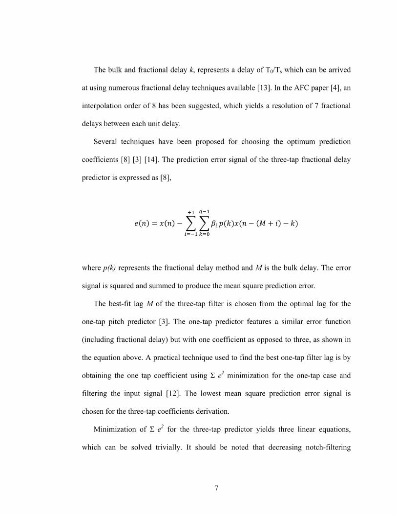
Several techniques have been proposed for choosing the optimum prediction
coefficients [8] [3] [14]. The prediction error signal of the three-tap fractional delay
predictor is expressed as [8],
! ! = ! ! − !!
!!!
!!!
!(!)!(! − ! + ! − !)!!
!!!!
where p(k) represents the fractional delay method and M is the bulk delay. The error
signal is squared and summed to produce the mean square prediction error.
The best-fit lag M of the three-tap filter is chosen from the optimal lag for the
one-tap pitch predictor [3]. The one-tap predictor features a similar error function
(including fractional delay) but with one coefficient as opposed to three, as shown in
the equation above. A practical technique used to find the best one-tap filter lag is by
obtaining the one tap coefficient using Σ e2 minimization for the one-tap case and
filtering the input signal [12]. The lowest mean square prediction error signal is
chosen for the three-tap coefficients derivation.
Minimization of Σ e2 for the three-tap predictor yields three linear equations,
which can be solved trivially. It should be noted that decreasing notch-filtering
8
spectrum with increasing frequency is guaranteed when the center coefficient is larger
than the side coefficients (representing β-1 and β1) [8]. This condition can be forced
by setting β0 coefficient to the one-tap predictor coefficient [3].
2.3. Issues in Real-Time Implementation
Processing of the input signal must be window based and real-time. A minimum
window length corresponds to at least two times the lowest expected fundamental
frequency. This is necessary in order to identify the input fundamental based on the
prediction error.
The AFC paper suggests the pitch search range to be from 100 Hz to 1 KHz. At
44.1 KHz sampling rate this corresponds to a minimum of 882-sample window.
On the other hand, an upper limit to the window size is the assumed short-term
stationarity of the signal. A window of 882 samples represents a 20ms time frame.
In addition, computational complexity of the algorithm as a function of window
length should be considered. Using an interpolation rate of 8 and a search range of
100 Hz to 1 KHz at 44.1 KHz sampling rate, 3176 total fractional delays are searched.
Using the practical approach to identifying the best lag M, this results in 3176
filtering operations to determine the prediction error.
The AFC paper suggests window size of 40 to 50ms. A window size of 2048,
corresponding to 46.4ms was chosen for the massively parallel implementation.
In the next chapter, simulation experiments are done to analyze the efficacy of the
whitening filters for a variety of expected input conditions.
9
Chapter 3 – Autoregressive and Pitch Prediction Filters Performance
In this chapter, the AR and PLP filters are implemented and tested against four
classes of input conditions. These input signals are meant to test the two filters against
various types of possible inputs. In a practical situation, the algorithm may receive an
infinite number of combinations of input conditions. Therefore, the discussion will focus
on a few important types.
The four classes of test signals consist of speech and audio signals. The goal of the
linear prediction filters is to model the input under diverse input conditions. The inverse
signal model is then used to suppress the dominant characteristics of the signal in order to
whiten the output. Most audio signals contain a periodic component in the spectrum but
typically will also contain a wideband aperiodic component as well. The ratio between
the two may not be known beforehand and may change from one sample window to the
next.
The first class of input signals is composed of synthesized test signals. Two
synthesized input signals are used to test the filters. The first input signal is classified as a
colored aperiodic signal and the second input signal is a synthesized Ab musical note. The
colored aperiodic signal will test the autoregressive filter independently, while the
synthesized musical note will test both independent and cascaded combinations of the AR
and PLP filters.
The second class of inputs consists of recorded speech signals. A recorded sibilance
signal of a male voice producing the sound ‘s’ is used to test the autoregressive filter. The
second speech signal is a recorded male voice producing the sound ‘ah’. The two speech
10
signals are tested with both independent AR and PLP filters and the cascaded
combination.
The third class of test inputs is the monophonic audio signal. This class of input
signals represents the target class of inputs in the AFC algorithm [4]. This test signal is a
recorded Ab piano note. The algorithm specifies a cascaded AR – PLP – AR filter
combination. Comparison of pre-whitening using the AR filter for the cascade PLP and
AR model filters will be done and compared to the non-prewhitened cascade structure.
The fourth and final class of test signals is the polyphonic audio signal. Two test
signals are used to test the cascade PLP and AR structure. The first is an Ab piano chord
and the second is an Ab piano chord with a bass note. No mention of the applicability of
the AFC algorithm to polyphonic signals is made in published AFC literature. Only a
brief analysis is done in this work. However, the extension of the whitening filters to
polyphonic signals is necessary due to the prevalence of polyphony in contemporary
music.
3.1. Test Filters Conditions
The two linear prediction filters being analyzed consist of a short (30-tap)
autoregressive and a pitch linear prediction filter. The autoregressive filter is
implemented using the autocorrelation method [7]. The PLP filter is implemented using
fractional delays (interpolation order = 8) with a pitch search range from 100 Hz to 1
KHz. Two types of PLP filters are compared, the 1-tap, 3-tap PLP filters, both of which
are fractionally delayed. The simplest of the two is the 1–tap PLP filter whose frequency
response has a uniform comb filter structure across the Nyquist bandwidth. The second
11
filter is the 3-tap filter, which finds the optimal bulk and fractional delay based on the
1-tap PLP residual and designs a 3-tap PLP filter based on the identified bulk and
fractional delay (using 3 degrees of freedom in the 3-tap coefficient least squares
minimization) [8].
The input signal is fractionally delayed using a polyphase interpolation FIR filter
structure with a 160-order low pass filter. The fractional delayed 1 and 3-tap filter
coefficients are derived using a 20 order delayed sinc interpolation [13].
All signals are sampled at 44.1 kHz and are 1024 samples in length (representing a
sample window of 23ms). Stationarity of the signal is assumed at these window lengths,
while no long-term stationarity is assumed. Therefore, each window pitch identification
search is done independently relative to previous iterations.
3.2. Test Metrics
Three primary test metrics are used to determine the efficacy of the whitening filters.
The first metric is kurtosis of the residual signal spectrum. This measure is used to
determine the degree to which the probability mass is distributed between the shoulders
of the distribution to its center [15]. Formally, it is defined as
! =!(! − !)!
!!
It is also known as the standardized fourth moment. It will be used here to measure
how outlier prone is the distribution of the spectrum of the residual signal. The fourth
12
power in the formula results in a wide variation in kurtosis of the test signals (between
single digits to hundreds). The normal distribution has a Kurtosis of 3. Lower values of
kurtosis signify whiter residual.
The second metric, the residual autocorrelation power weight (RAPW), measures the
degree of aperiodicity of the residual in the autocorrelation power domain. It can be
stated as the ratio of the power of the zero order autocorrelation with respect to the mean
power of all remaining autocorrelation lags. Higher values signify a whiter residual
spectrum.
!"#$ = !"#$%$&&(!, 0) !
1! !"#$%$&&(!, !) !!!!
!!!
The third and final test metric is the residual spectral flatness measure (SFM). This
measure was introduced by Gray and Markel [16] and is common in audio signals
whitening literature [12]. This measure examines the average spread of the spectrum in
the frequency domain.
!"# =!"# (1/!) ln ! !!!!!/! , !!!!
!!!
(1!) ! !!!!"/! , !!!!!!!
It is normalized so that a white residual spectrum has an SFM of 1. Values of SFM
are always positive.
13
3.3. Synthesized Test Signals
The AR and PLP filters are tested using synthesized models of real inputs. If the filter
performs well against these test signals, real input signals can then be used to test the
filters. This ensures that the filter behaves as expected against the modeled test signals.
The first class of test signals represents synthesized colored noise and a synthesized Ab
musical note.
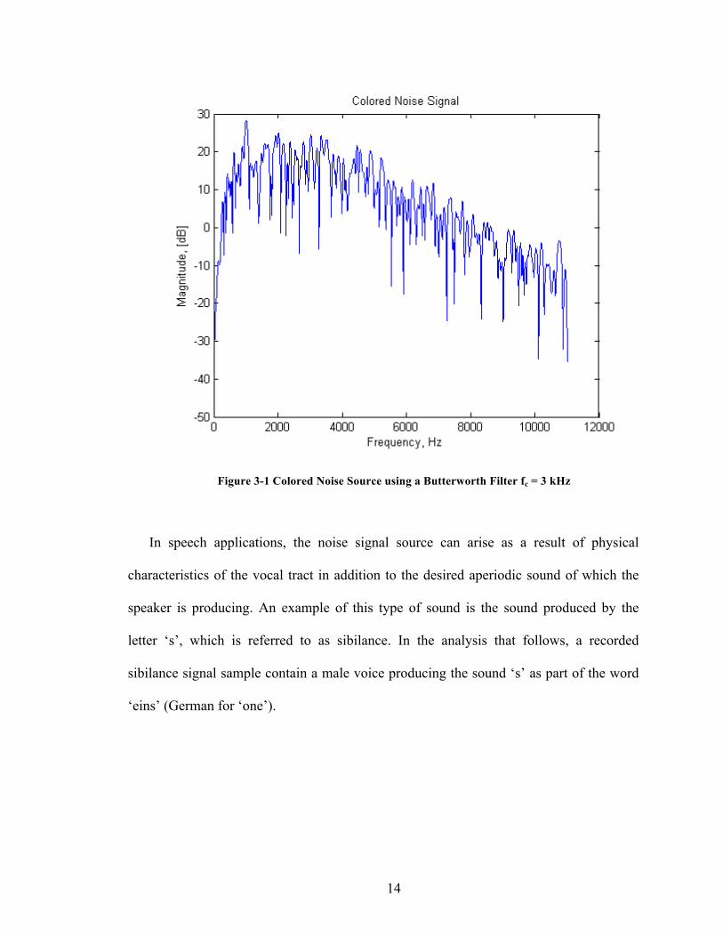
3.3.1. Colored Noise
The first category of input signals is colored noise. In a practical situation, the source
of noise can be electrical and acoustic. In reality, the noise signal itself may be a desirable
aperiodic aspect of the input signal (e.g. guitar distortion). In acoustic musical
instruments, the presence of the aperiodic signal identifies the difference in quality
between two identical instrument types, or two different musicians. It may be helpful to
identify colored noise in this context as being the wide band aperiodic signal of which the
pitch of the harmonics of the tone dominates when viewed in the frequency domain.
14
Figure 3-1 Colored Noise Source using a Butterworth Filter fc = 3 kHz
In speech applications, the noise signal source can arise as a result of physical
characteristics of the vocal tract in addition to the desired aperiodic sound of which the
speaker is producing. An example of this type of sound is the sound produced by the
letter ‘s’, which is referred to as sibilance. In the analysis that follows, a recorded
sibilance signal sample contain a male voice producing the sound ‘s’ as part of the word
‘eins’ (German for ‘one’).
15
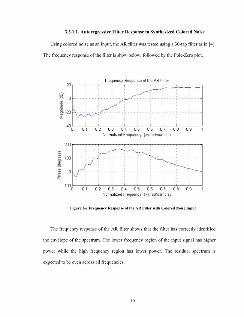
3.3.1.1. Autoregressive Filter Response to Synthesized Colored Noise
Using colored noise as an input, the AR filter was tested using a 30-tap filter as in [4].
The frequency response of the filter is show below, followed by the Pole-Zero plot.
Figure 3-2 Frequency Response of the AR Filter with Colored Noise Input
The frequency response of the AR filter shows that the filter has correctly identified
the envelope of the spectrum. The lower frequency region of the input signal has higher
power while the high frequency region has lower power. The residual spectrum is
expected to be even across all frequencies.
16
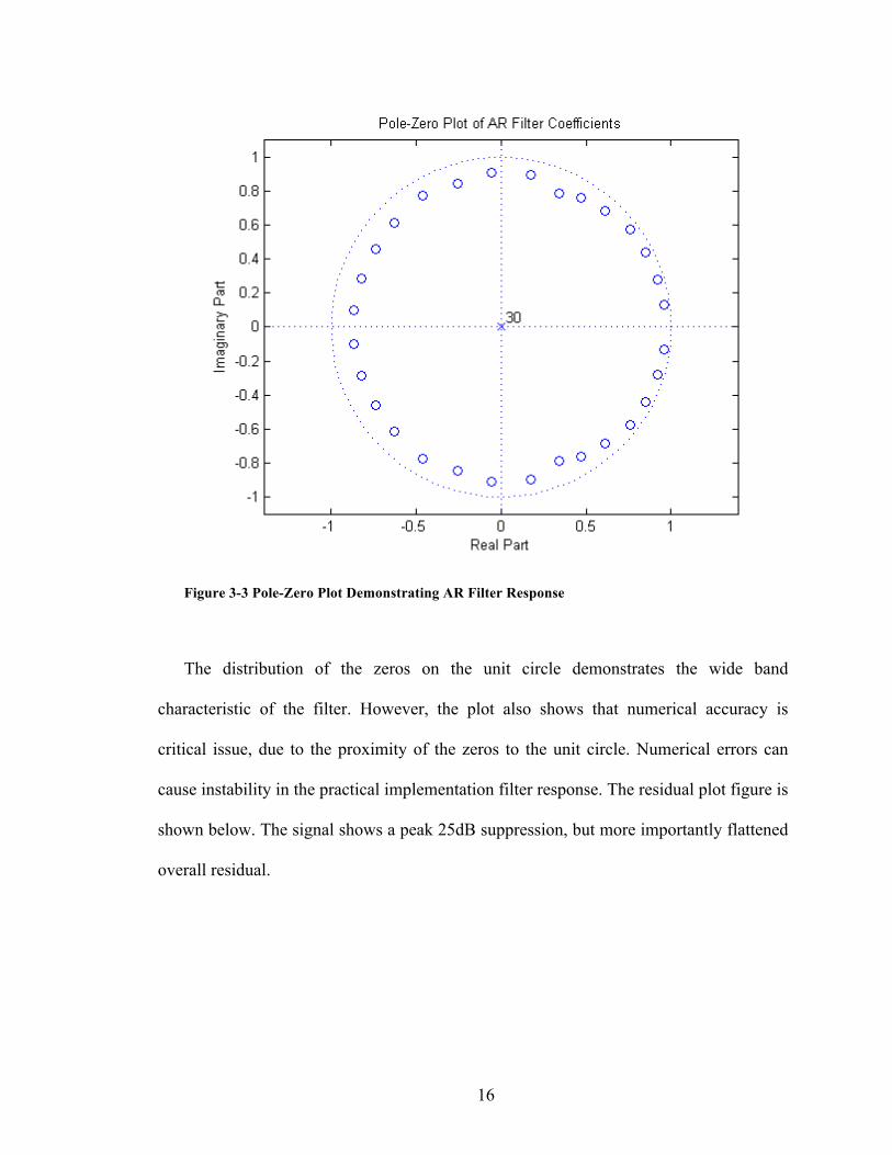
Figure 3-3 Pole-Zero Plot Demonstrating AR Filter Response
The distribution of the zeros on the unit circle demonstrates the wide band
characteristic of the filter. However, the plot also shows that numerical accuracy is
critical issue, due to the proximity of the zeros to the unit circle. Numerical errors can
cause instability in the practical implementation filter response. The residual plot figure is
shown below. The signal shows a peak 25dB suppression, but more importantly flattened
overall residual.
17
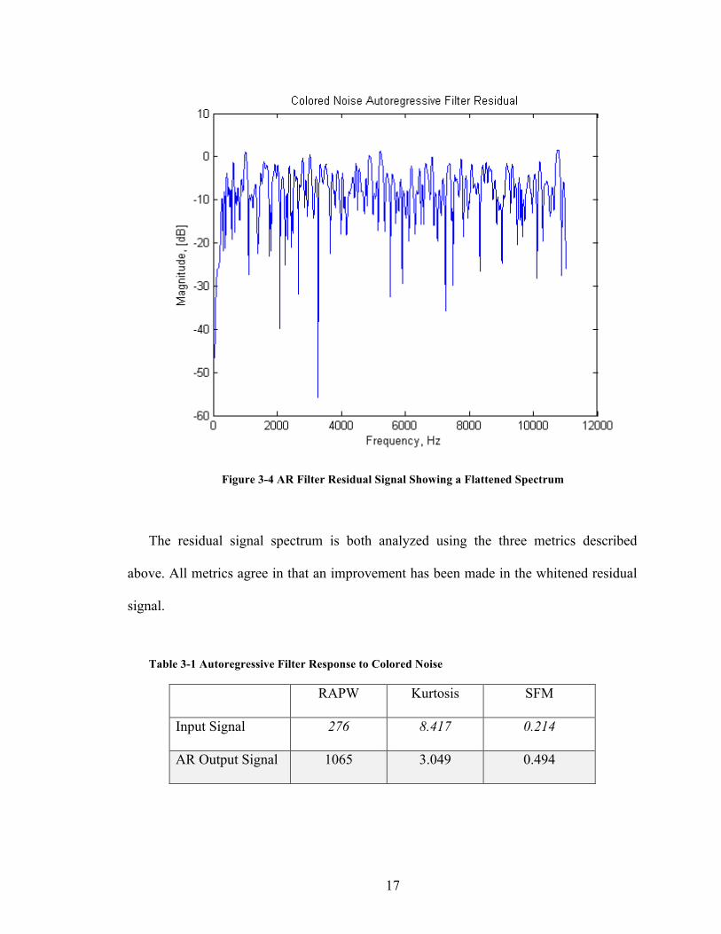
Figure 3-4 AR Filter Residual Signal Showing a Flattened Spectrum
The residual signal spectrum is both analyzed using the three metrics described
above. All metrics agree in that an improvement has been made in the whitened residual
signal.
Table 3-1 Autoregressive Filter Response to Colored Noise
RAPW Kurtosis SFM
Input Signal 276 8.417 0.214
AR Output Signal 1065 3.049 0.494
18
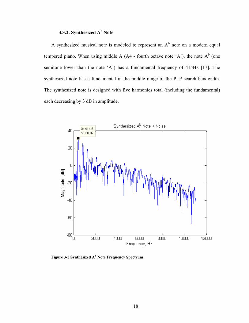
3.3.2. Synthesized Ab Note
A synthesized musical note is modeled to represent an Ab note on a modern equal
tempered piano. When using middle A (A4 - fourth octave note ‘A’), the note Ab (one
semitone lower than the note ‘A’) has a fundamental frequency of 415Hz [17]. The
synthesized note has a fundamental in the middle range of the PLP search bandwidth.
The synthesized note is designed with five harmonics total (including the fundamental)
each decreasing by 3 dB in amplitude.
Figure 3-5 Synthesized Ab Note Frequency Spectrum
19
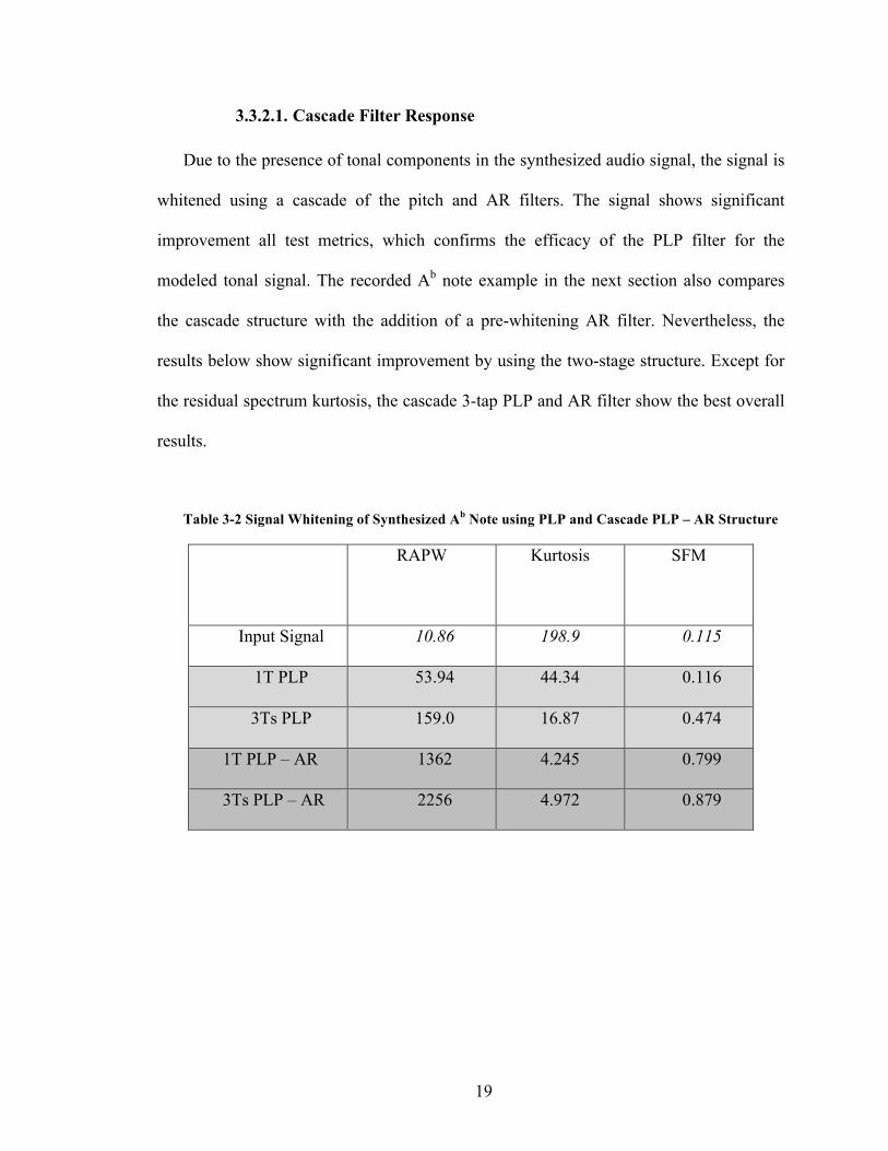
3.3.2.1. Cascade Filter Response
Due to the presence of tonal components in the synthesized audio signal, the signal is
whitened using a cascade of the pitch and AR filters. The signal shows significant
improvement all test metrics, which confirms the efficacy of the PLP filter for the
modeled tonal signal. The recorded Ab note example in the next section also compares
the cascade structure with the addition of a pre-whitening AR filter. Nevertheless, the
results below show significant improvement by using the two-stage structure. Except for
the residual spectrum kurtosis, the cascade 3-tap PLP and AR filter show the best overall
results.
Table 3-2 Signal Whitening of Synthesized Ab Note using PLP and Cascade PLP – AR Structure
RAPW Kurtosis SFM
Input Signal 10.86 198.9 0.115
1T PLP 53.94 44.34 0.116
3Ts PLP 159.0 16.87 0.474
1T PLP – AR 1362 4.245 0.799
3Ts PLP – AR 2256 4.972 0.879
20
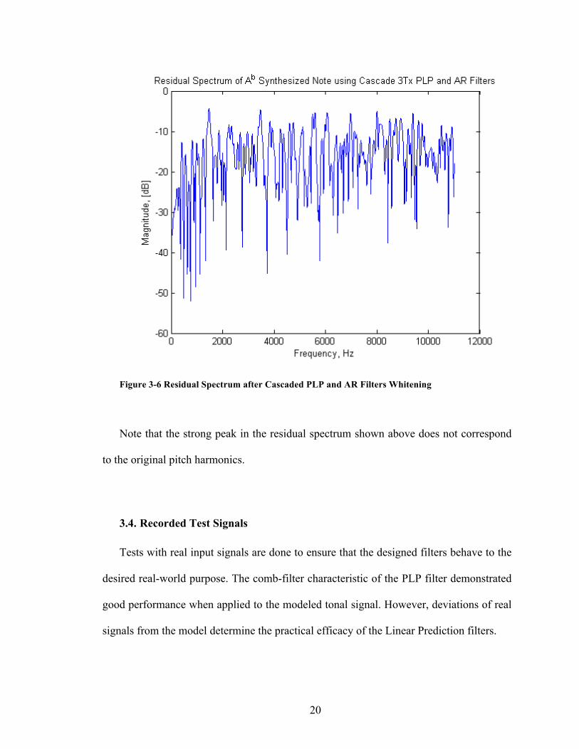
Figure 3-6 Residual Spectrum after Cascaded PLP and AR Filters Whitening
Note that the strong peak in the residual spectrum shown above does not correspond
to the original pitch harmonics.
3.4. Recorded Test Signals
Tests with real input signals are done to ensure that the designed filters behave to the
desired real-world purpose. The comb-filter characteristic of the PLP filter demonstrated
good performance when applied to the modeled tonal signal. However, deviations of real
signals from the model determine the practical efficacy of the Linear Prediction filters.
21
A set of speech signals is tested first. Both the PLP and AR filters were first
introduced for speech filtering applications, and enjoy wide use in speech coding
applications [8] and are expected to perform well with recorded speech signals.
Recorded musical notes are then tested to determine the efficacy of the approach to
music signals. The recorded music signals are all piano recordings. These signals
comprise of both monophonic and polyphonic test signals.
3.4.1. Recorded Speech Signals
Two recorded male voice speech signals are used. The first signal will be used to test
the autoregressive filter. This signal is a recorded sibilance and the second signal is a
vocalization of the vowel ‘ah’ which will be used to test the PLP filter as well.
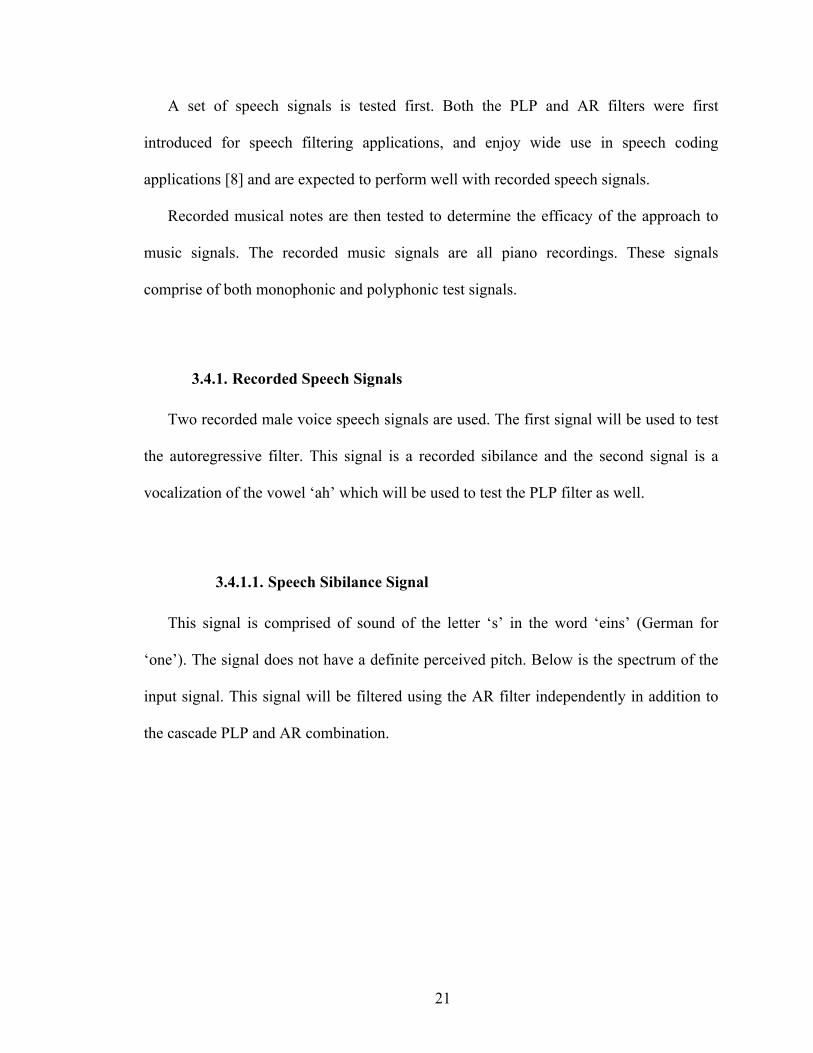
3.4.1.1. Speech Sibilance Signal
This signal is comprised of sound of the letter ‘s’ in the word ‘eins’ (German for
‘one’). The signal does not have a definite perceived pitch. Below is the spectrum of the
input signal. This signal will be filtered using the AR filter independently in addition to
the cascade PLP and AR combination.
22
Figure 3-7 Recorded 's' Sound from a Male Voice
3.4.1.1.1. Autoregressive Filter Response to Recorded ‘s’ Sound
After AR filtering, the signal shows large improvement in overall whitening. The 30-
Tap AR filter was able to model the envelope characteristics of the signal, which shows
higher spectral complexity compared to the original synthesized colored noise signal. The
cascade PLP and AR filters are also compared in order to determine if the structure can
remain fixed without consideration for the type of input signal received.
23
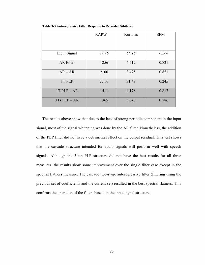
Table 3-3 Autoregressive Filter Response to Recorded Sibilance
RAPW Kurtosis SFM
Input Signal 37.76 65.18 0.268
AR Filter 1256 4.512 0.821
AR – AR 2100 3.475 0.851
1T PLP 77.03 31.49 0.245
1T PLP – AR 1411 4.178 0.817
3Ts PLP – AR 1365 3.640 0.786
The results above show that due to the lack of strong periodic component in the input
signal, most of the signal whitening was done by the AR filter. Nonetheless, the addition
of the PLP filter did not have a detrimental effect on the output residual. This test shows
that the cascade structure intended for audio signals will perform well with speech
signals. Although the 3-tap PLP structure did not have the best results for all three
measures, the results show some improvement over the single filter case except in the
spectral flatness measure. The cascade two-stage autoregressive filter (filtering using the
previous set of coefficients and the current set) resulted in the best spectral flatness. This
confirms the operation of the filters based on the input signal structure.
24
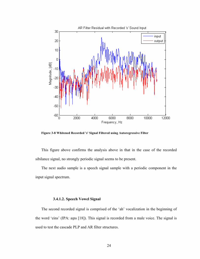
Figure 3-8 Whitened Recorded 's' Signal Filtered using Autoregressive Filter
This figure above confirms the analysis above in that in the case of the recorded
sibilance signal, no strongly periodic signal seems to be present.
The next audio sample is a speech signal sample with a periodic component in the
input signal spectrum.
3.4.1.2. Speech Vowel Signal
The second recorded signal is comprised of the ‘ah’ vocalization in the beginning of
the word ‘eins’ (IPA: aɪ̯ns [18]). This signal is recorded from a male voice. The signal is
used to test the cascade PLP and AR filter structures.
25
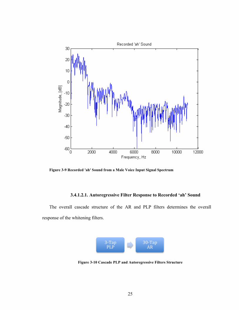
Figure 3-9 Recorded 'ah' Sound from a Male Voice Input Signal Spectrum
3.4.1.2.1. Autoregressive Filter Response to Recorded ‘ah’ Sound
The overall cascade structure of the AR and PLP filters determines the overall
response of the whitening filters.
Figure 3-10 Cascade PLP and Autoregressive Filters Structure
3-‐Tap PLP
30-‐Tap AR
26
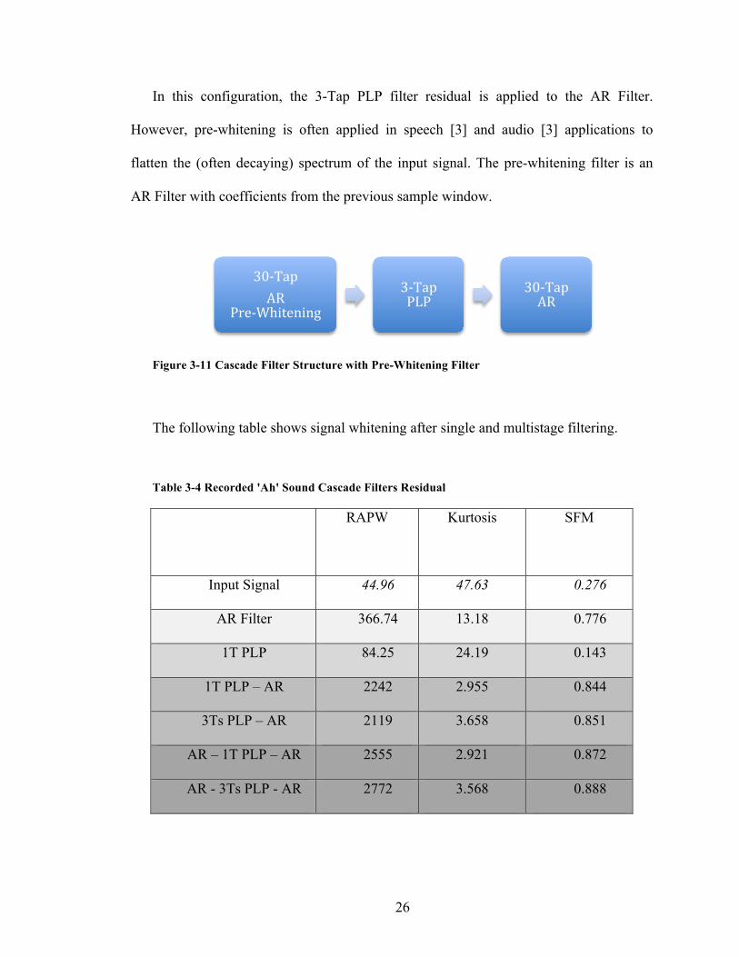
In this configuration, the 3-Tap PLP filter residual is applied to the AR Filter.
However, pre-whitening is often applied in speech [3] and audio [3] applications to
flatten the (often decaying) spectrum of the input signal. The pre-whitening filter is an
AR Filter with coefficients from the previous sample window.
Figure 3-11 Cascade Filter Structure with Pre-Whitening Filter
The following table shows signal whitening after single and multistage filtering.
Table 3-4 Recorded 'Ah' Sound Cascade Filters Residual
RAPW Kurtosis SFM
Input Signal 44.96 47.63 0.276
AR Filter 366.74 13.18 0.776
1T PLP 84.25 24.19 0.143
1T PLP – AR 2242 2.955 0.844
3Ts PLP – AR 2119 3.658 0.851
AR – 1T PLP – AR 2555 2.921 0.872
AR - 3Ts PLP - AR 2772 3.568 0.888
30-‐Tap AR
Pre-‐Whitening
3-‐Tap PLP
30-‐Tap AR
27
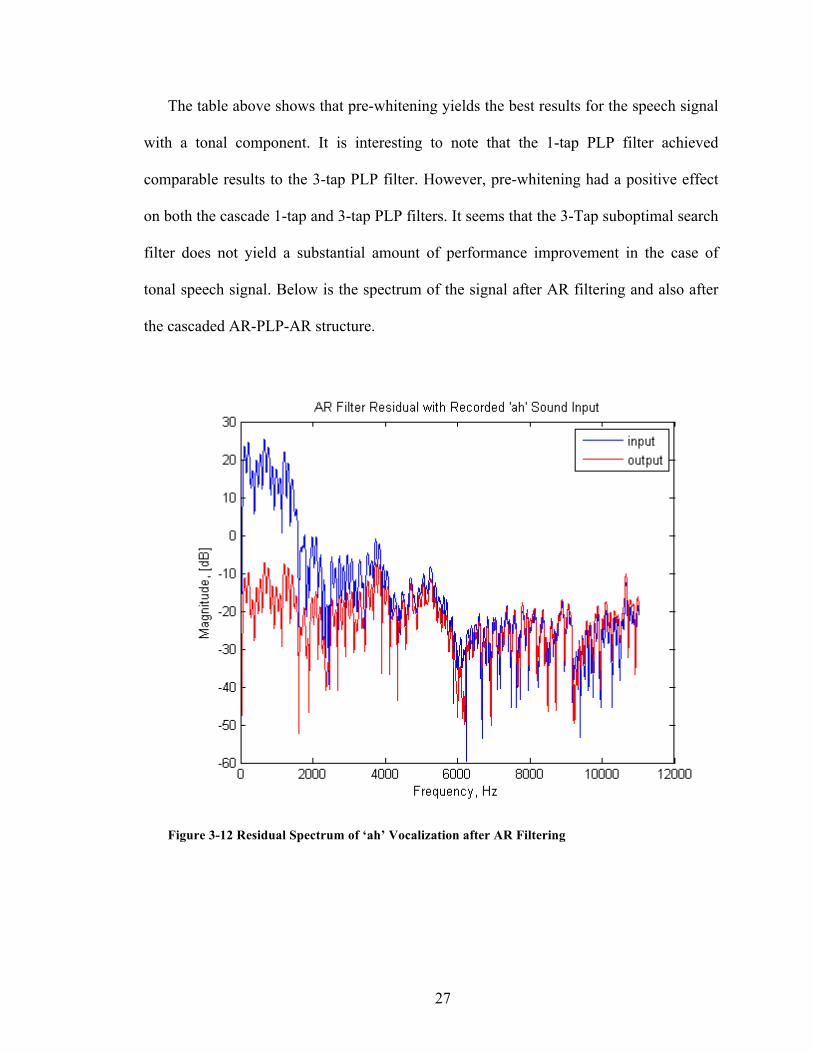
The table above shows that pre-whitening yields the best results for the speech signal
with a tonal component. It is interesting to note that the 1-tap PLP filter achieved
comparable results to the 3-tap PLP filter. However, pre-whitening had a positive effect
on both the cascade 1-tap and 3-tap PLP filters. It seems that the 3-Tap suboptimal search
filter does not yield a substantial amount of performance improvement in the case of
tonal speech signal. Below is the spectrum of the signal after AR filtering and also after
the cascaded AR-PLP-AR structure.
Figure 3-12 Residual Spectrum of ‘ah’ Vocalization after AR Filtering
28
The figure above shows the persistence of the tonal components in the signal
spectrum after the AR filter. This is expected since the AR filter is meant to flatten the
general envelope of the complete spectrum.
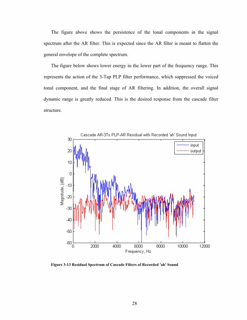
The figure below shows lower energy in the lower part of the frequency range. This
represents the action of the 3-Tap PLP filter performance, which suppressed the voiced
tonal component, and the final stage of AR filtering. In addition, the overall signal
dynamic range is greatly reduced. This is the desired response from the cascade filter
structure.
Figure 3-13 Residual Spectrum of Cascade Filters of Recorded 'ah' Sound
29
The mixture of strongly periodic characteristics and decaying broadband aperiodic
component is typical for many recorded signals; as will be evident from the following
audio samples. In the example above, the final output of cascade filters shows a dynamic
range of approximately 15dB compared to the input signal dynamic range of 55dB.
3.4.2. Recorded Musical Notes
First, analysis of monophonic input signals is discussed followed by polyphonic audio
samples. Musical notes are expected to have a more complex spectrum when compared to
speech signals. The strength of the periodic to the aperiodic components is another factor
that should be identified.
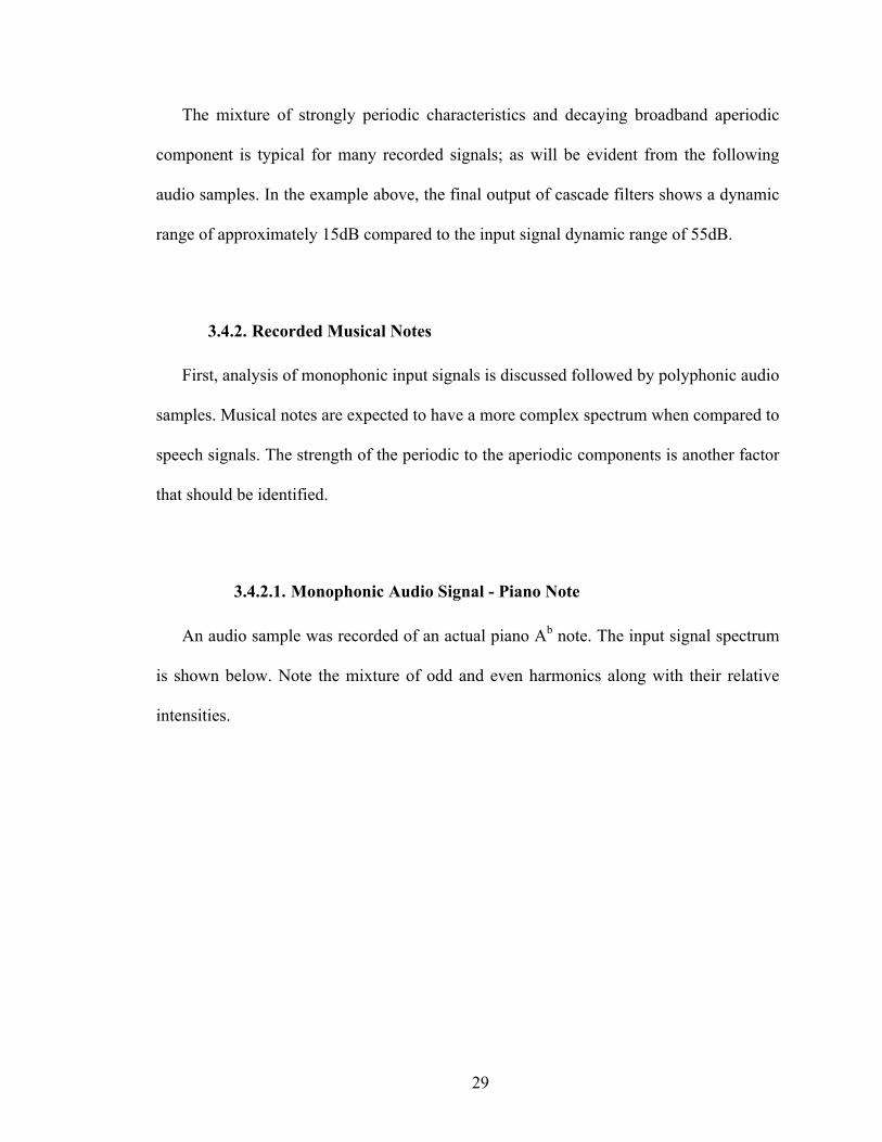
3.4.2.1. Monophonic Audio Signal - Piano Note
An audio sample was recorded of an actual piano Ab note. The input signal spectrum
is shown below. Note the mixture of odd and even harmonics along with their relative
intensities.
30
Figure 3-14 Recorded Ab Piano Note
The spectrum shows a complex harmonic structure that extends beyond 15
harmonics. The fundamental is at approximately 415Hz, which is within the search range
of the PLP filter. The input signal dynamic range is approximately 70dB.
3.4.2.1.1. Cascade Pitch and Autoregressive Response – Monophonic
Input Signal
Below is a table showing the results of cascade filtering with and without pre-
whitening filter. The cascade structure with pre-whitening shows a slight improvement in
31
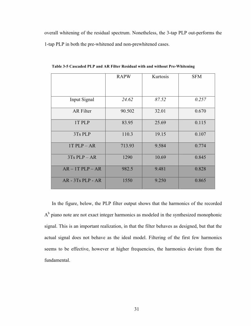
overall whitening of the residual spectrum. Nonetheless, the 3-tap PLP out-performs the
1-tap PLP in both the pre-whitened and non-prewhitened cases.
Table 3-5 Cascaded PLP and AR Filter Residual with and without Pre-Whitening
RAPW Kurtosis SFM
Input Signal 24.62 87.52 0.257
AR Filter 90.502 32.01 0.670
1T PLP 83.95 25.69 0.115
3Ts PLP 110.3 19.15 0.107
1T PLP – AR 713.93 9.584 0.774
3Ts PLP – AR 1290 10.69 0.845
AR – 1T PLP – AR 982.5 9.481 0.828
AR - 3Ts PLP - AR 1550 9.250 0.865
In the figure, below, the PLP filter output shows that the harmonics of the recorded
Ab piano note are not exact integer harmonics as modeled in the synthesized monophonic
signal. This is an important realization, in that the filter behaves as designed, but that the
actual signal does not behave as the ideal model. Filtering of the first few harmonics
seems to be effective, however at higher frequencies, the harmonics deviate from the
fundamental.
32
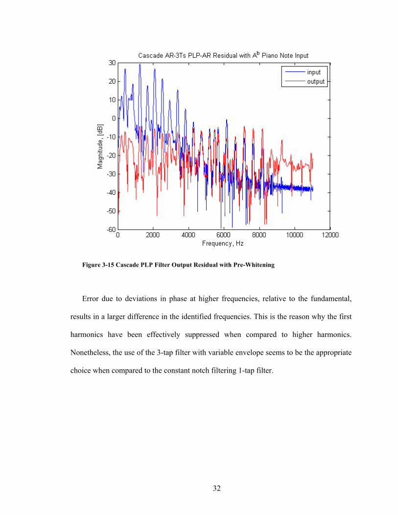
Figure 3-15 Cascade PLP Filter Output Residual with Pre-Whitening
Error due to deviations in phase at higher frequencies, relative to the fundamental,
results in a larger difference in the identified frequencies. This is the reason why the first
harmonics have been effectively suppressed when compared to higher harmonics.
Nonetheless, the use of the 3-tap filter with variable envelope seems to be the appropriate
choice when compared to the constant notch filtering 1-tap filter.
33
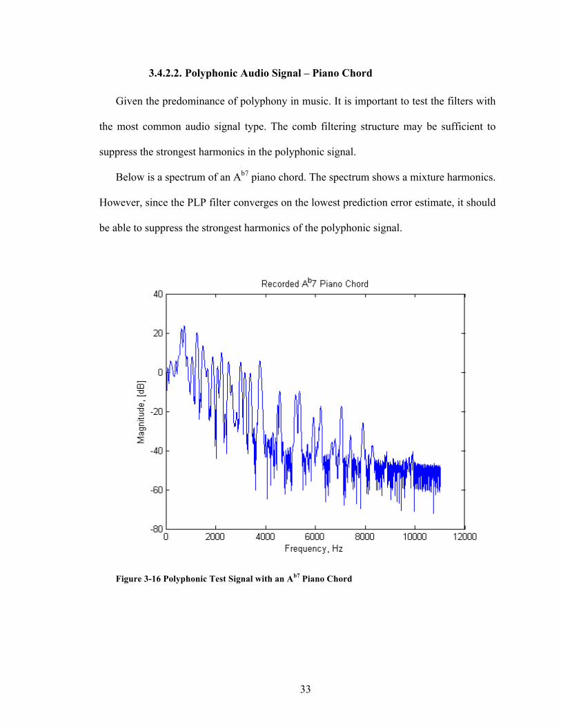
3.4.2.2. Polyphonic Audio Signal – Piano Chord
Given the predominance of polyphony in music. It is important to test the filters with
the most common audio signal type. The comb filtering structure may be sufficient to
suppress the strongest harmonics in the polyphonic signal.
Below is a spectrum of an Ab7 piano chord. The spectrum shows a mixture harmonics.
However, since the PLP filter converges on the lowest prediction error estimate, it should
be able to suppress the strongest harmonics of the polyphonic signal.
Figure 3-16 Polyphonic Test Signal with an Ab7 Piano Chord
34
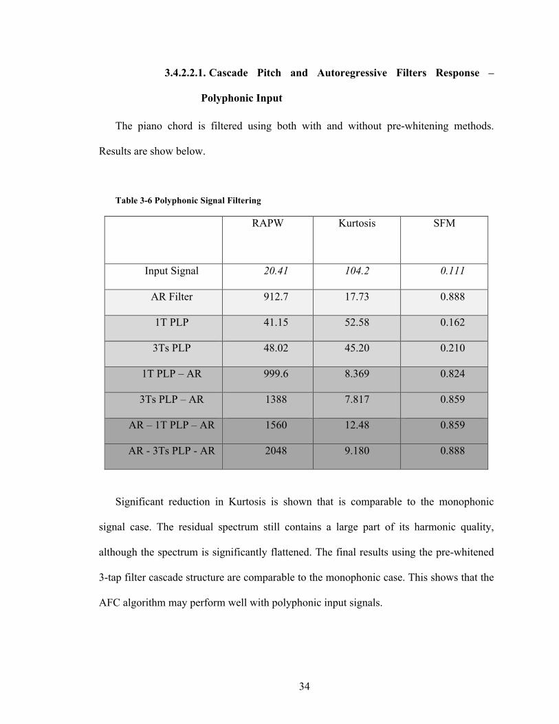
3.4.2.2.1. Cascade Pitch and Autoregressive Filters Response –
Polyphonic Input
The piano chord is filtered using both with and without pre-whitening methods.
Results are show below.
Table 3-6 Polyphonic Signal Filtering
RAPW Kurtosis SFM
Input Signal 20.41 104.2 0.111
AR Filter 912.7 17.73 0.888
1T PLP 41.15 52.58 0.162
3Ts PLP 48.02 45.20 0.210
1T PLP – AR 999.6 8.369 0.824
3Ts PLP – AR 1388 7.817 0.859
AR – 1T PLP – AR 1560 12.48 0.859
AR - 3Ts PLP - AR 2048 9.180 0.888
Significant reduction in Kurtosis is shown that is comparable to the monophonic
signal case. The residual spectrum still contains a large part of its harmonic quality,
although the spectrum is significantly flattened. The final results using the pre-whitened
3-tap filter cascade structure are comparable to the monophonic case. This shows that the
AFC algorithm may perform well with polyphonic input signals.

35
Figure 3-17 Cascade PLP and AR Filters Residual for Ab7 Chord Polyphonic Input
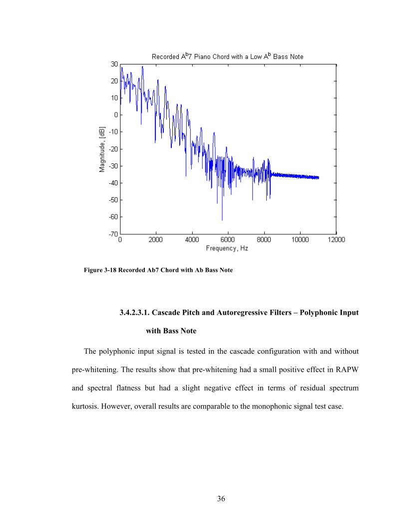
3.4.2.3. Polyphonic Audio Signal – Piano Chord with Bass Note
In addition, a piano chord (same as in the previous section) with a bass note is used to
test if the bass note helps in the PLP algorithm’s identification. The bass note is an Ab2
(second octave Ab, with approximately 103Hz fundamental frequency [17]).
36
Figure 3-18 Recorded Ab7 Chord with Ab Bass Note
3.4.2.3.1. Cascade Pitch and Autoregressive Filters – Polyphonic Input
with Bass Note
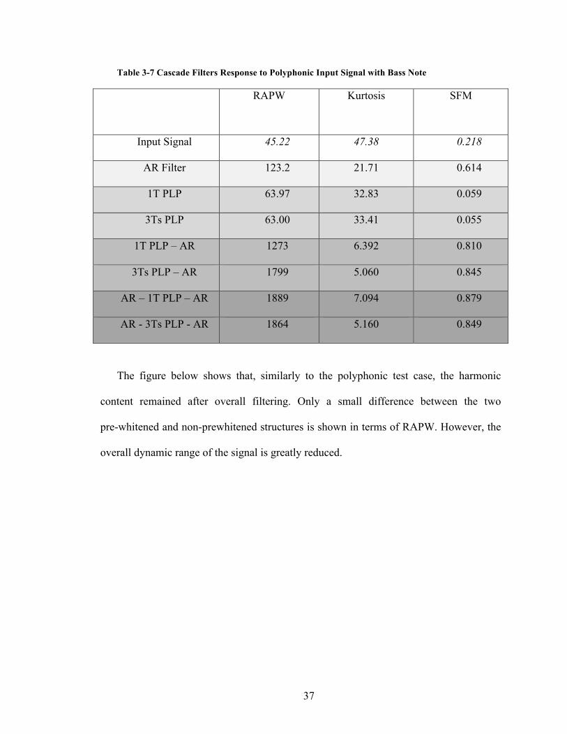
The polyphonic input signal is tested in the cascade configuration with and without
pre-whitening. The results show that pre-whitening had a small positive effect in RAPW
and spectral flatness but had a slight negative effect in terms of residual spectrum
kurtosis. However, overall results are comparable to the monophonic signal test case.
37
Table 3-7 Cascade Filters Response to Polyphonic Input Signal with Bass Note
RAPW Kurtosis SFM
Input Signal 45.22 47.38 0.218
AR Filter 123.2 21.71 0.614
1T PLP 63.97 32.83 0.059
3Ts PLP 63.00 33.41 0.055
1T PLP – AR 1273 6.392 0.810
3Ts PLP – AR 1799 5.060 0.845
AR – 1T PLP – AR 1889 7.094 0.879
AR - 3Ts PLP - AR 1864 5.160 0.849
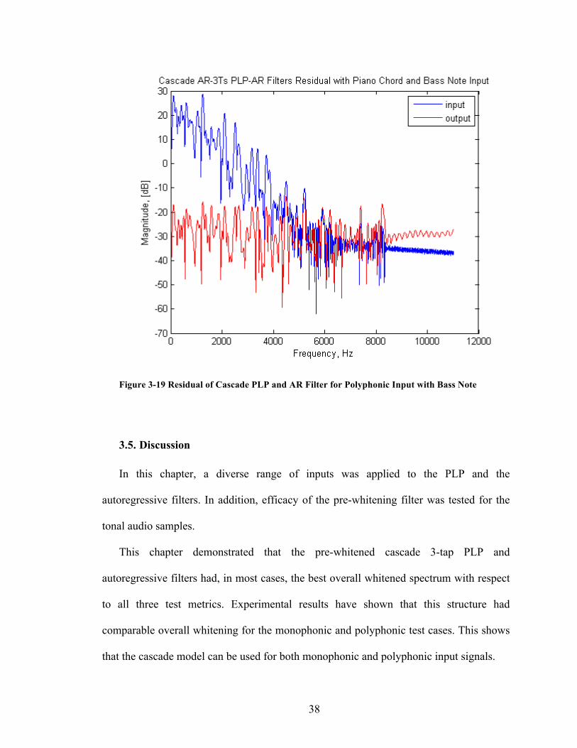
The figure below shows that, similarly to the polyphonic test case, the harmonic
content remained after overall filtering. Only a small difference between the two
pre-whitened and non-prewhitened structures is shown in terms of RAPW. However, the
overall dynamic range of the signal is greatly reduced.
38
Figure 3-19 Residual of Cascade PLP and AR Filter for Polyphonic Input with Bass Note
3.5. Discussion
In this chapter, a diverse range of inputs was applied to the PLP and the
autoregressive filters. In addition, efficacy of the pre-whitening filter was tested for the
tonal audio samples.
This chapter demonstrated that the pre-whitened cascade 3-tap PLP and
autoregressive filters had, in most cases, the best overall whitened spectrum with respect
to all three test metrics. Experimental results have shown that this structure had
comparable overall whitening for the monophonic and polyphonic test cases. This shows
that the cascade model can be used for both monophonic and polyphonic input signals.
39
One important finding is that experimental results have shown that harmonics of
recorded audio signals are not necessarily related by an integer number. This degraded
the performance of the comb filter at higher frequencies. One possible reason may be due
to the frequency resolution of the interpolated 3-tap PLP filter. Karpus and Strong [19]
have shown that musical instrument modeling can be achieved using fractional delays
and 30 sine wave generators to produce a realistic timbre. Modification of the comb filter
to have a wider bandwidth and increased suppression would be desirable for real test
signals. This is because recorded monophonic and polyphonic signals have shown that
the tonal components of test signals are significantly stronger than the aperiodic
components.
40
Chapter 4 – DSP Implementation
Migration of the linear prediction filters to an embedded DSP processor depends on
the capability and resources available in the embedded architecture. The autoregressive
filter requires solving the Yule-Walker equations using matrix inversion. The 3-Tap PLP
filter requires the calculation of the residual mean square prediction error for each search
interval in order to find the best-fit coefficients.
4.1. Challenges in Implementation
The autoregressive filter does not require as much memory as the PLP filter.
However, it requires inverting a 30x30 reflection coefficients matrix [19]. This can
present a significant amount of computation, which may prevent the algorithm from
achieving real-time performance.
Two matrix inversion methods will be investigated, the first is the Levinson-Durbin
recursion, which requires O(n2) computations [3]. The second matrix inversion method is
the Gauss-Jordan method, which requires O(n3) computations [20].
In the 3-tap PLP filter implementation, memory consumption is an important issue.
This is because the large search region of the filter and 8 times interpolation that is
required. Many implementations exist [21] for fractional interpolation. Polyphase FIR
was chosen due to the fact that one filter can be used to produce all eight fractional
delays. It is important to note that the FIR input and output signal length required is eight
times the original window size (for a 1024 sample window in the DSP implementation
resulted in an 8192 output signal). On the other hand, this implementation makes all eight
41
fractional delays available for the entire search region using one filter (through the use of
multiple starting positions for the output and increment in the address by the interpolation
order).
4.2. Target Architecture
The chosen processor for the hardware implementation is the Analog Devices
SHARC 21369 400MHz Floating Point DSP processor. The processor uses a modified
Harvard architecture with separate data and instruction buses. The processor allows
SIMD-Single Instruction Multiple Data, which is beneficial for fast FIR processing. The
processor contains two computational units that allow simultaneous computation of an
instruction on two sets of data. The combination of SIMD and modified Harvard
architecture allow four operands and one instruction fetch in a single cycle.
On chip memory is made up of 2Mbit shared program and data memory (allows total
65k 32-bit words). In order to exploit SIMD, data and program instructions must be
located in their respective memory regions. The processor also contains two data address
generators that support circular buffers in hardware.
4.3. DSP Processor vs FPGA
The floating point DSP processor was chosen over an FPGA implementation. In
addition to the difficulty presented in fixed-point implementation, FPGAs tend to be
slower than DSP processors in terms of core clock speeds. In addition, parallel
computation would not have been possible with a low-cost FPGA device. Xu et al [13]
42
have shown that implementation of Levinson-Durbin algorithm for coefficients
calculation in speech applications consumes 16,254 Configurable Logic Blocks (CLB) on
a Xilinx Virtex-E device. In their implementation, the maximum clock frequency was
limited to 13.4MHz. Notwithstanding the fact that the 3-Tap PLP filter has significantly
higher computational complexity compared to the autoregressive filter. Therefore, a DSP
processor implementation is more likely to be able to achieve real-time performance.
4.4. DSP Processor Performance Results
In the DSP processor implementation, the window length was limited to 1024
samples. This was done in order to reduce overall memory consumption. The window
size allows holding in memory up to a maximum of two periods for the lowest frequency
in the search window (100Hz, 441 samples at 44.1 KHz sample rate). The MATLAB
comparison results are generated using the same 1024 sample window.
The polyphase interpolation ratio was kept at 8 times similar to the MATLAB
simulations in the previous chapter. Also, the autoregressive filter was set to 30-taps and
the 3-Tap PLP filter was set to search from 44 to 441 samples (with 8 fractional delays).
The 3-Tap PLP filter was set to 3 degrees of freedom in the coefficient estimation.
4.4.1. Recorded Sibilance – AR Filter Testing
The recorded male voice vocalization of ‘s’ as analyzed in the previous chapter was
used in the Autoregressive filter testing. The filter was tested using a 1024 sample
window.
43
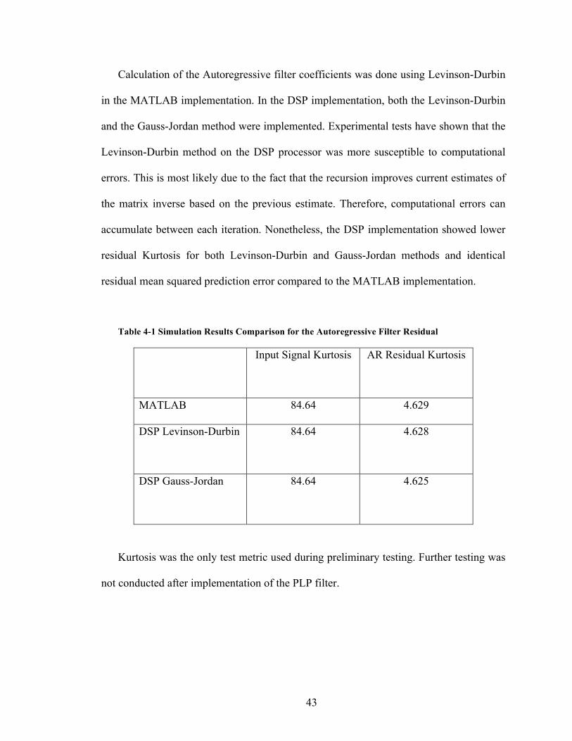
Calculation of the Autoregressive filter coefficients was done using Levinson-Durbin
in the MATLAB implementation. In the DSP implementation, both the Levinson-Durbin
and the Gauss-Jordan method were implemented. Experimental tests have shown that the
Levinson-Durbin method on the DSP processor was more susceptible to computational
errors. This is most likely due to the fact that the recursion improves current estimates of
the matrix inverse based on the previous estimate. Therefore, computational errors can
accumulate between each iteration. Nonetheless, the DSP implementation showed lower
residual Kurtosis for both Levinson-Durbin and Gauss-Jordan methods and identical
residual mean squared prediction error compared to the MATLAB implementation.
Table 4-1 Simulation Results Comparison for the Autoregressive Filter Residual
Input Signal Kurtosis AR Residual Kurtosis
MATLAB 84.64 4.629
DSP Levinson-Durbin 84.64 4.628
DSP Gauss-Jordan 84.64 4.625
Kurtosis was the only test metric used during preliminary testing. Further testing was
not conducted after implementation of the PLP filter.
44
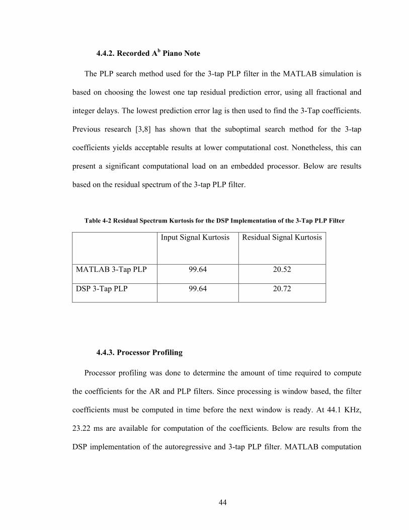
4.4.2. Recorded Ab Piano Note
The PLP search method used for the 3-tap PLP filter in the MATLAB simulation is
based on choosing the lowest one tap residual prediction error, using all fractional and
integer delays. The lowest prediction error lag is then used to find the 3-Tap coefficients.
Previous research [3,8] has shown that the suboptimal search method for the 3-tap
coefficients yields acceptable results at lower computational cost. Nonetheless, this can
present a significant computational load on an embedded processor. Below are results
based on the residual spectrum of the 3-tap PLP filter.
Table 4-2 Residual Spectrum Kurtosis for the DSP Implementation of the 3-Tap PLP Filter
Input Signal Kurtosis Residual Signal Kurtosis
MATLAB 3-Tap PLP 99.64 20.52
DSP 3-Tap PLP 99.64 20.72
4.4.3. Processor Profiling
Processor profiling was done to determine the amount of time required to compute
the coefficients for the AR and PLP filters. Since processing is window based, the filter
coefficients must be computed in time before the next window is ready. At 44.1 KHz,
23.22 ms are available for computation of the coefficients. Below are results from the
DSP implementation of the autoregressive and 3-tap PLP filter. MATLAB computation
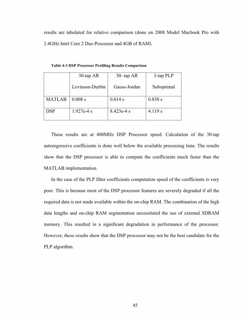
45
results are tabulated for relative comparison (done on 2008 Model Macbook Pro with
2.4GHz Intel Core 2 Duo Processor and 4GB of RAM).
Table 4-3 DSP Processor Profiling Results Comparison
30-tap AR
Levinson-Durbin
30- tap AR
Gauss-Jordan
3-tap PLP
Suboptimal
MATLAB 0.008 s 0.014 s 0.838 s
DSP 1.927e-4 s 8.423e-4 s 4.119 s
These results are at 400MHz DSP Processor speed. Calculation of the 30-tap
autoregressive coefficients is done well below the available processing time. The results
show that the DSP processor is able to compute the coefficients much faster than the
MATLAB implementation.
In the case of the PLP filter coefficients computation speed of the coefficients is very
poor. This is because most of the DSP processor features are severely degraded if all the
required data is not made available within the on-chip RAM. The combination of the high
data lengths and on-chip RAM segmentation necessitated the use of external SDRAM
memory. This resulted in a significant degradation in performance of the processor.
However, these results show that the DSP processor may not be the best candidate for the
PLP algorithm.
46
4.5. Problems Encountered
Most problems in the DSP implementation were related to memory constraints. Since
the processor is a floating-point processor, few numerical issues were encountered.
Nonetheless, hardware division accuracy was a problem when computing the
autoregressive filter coefficients.
4.5.1. Memory Segmentation
The processor specification sheet lists the DSP chip as having 2Mbits of RAM,
which should be sufficient for this algorithm. Unfortunately, the memory is
segmented in to four blocks. Two blocks held .75Mbits or RAM while the second two
held .25Mbits. The two .25Mbits memory blocks held program stack and heap
(separately). In addition, on-chip RAM is used to store the actual program. One of the
.75Mbits memory blocks held program code. This combination made memory
management very challenging. The new generation SHARC processors, although run
at a maximum of 400MHz, contain 5Mbits of onboard memory (separated in to two
memory blocks), in addition to having FIR, IIR and FFT hardware accelerators.
4.5.2. Stack Overflow
The DSP processor experienced stack overflow only when a function is called that
contains large data vectors. However, the problem disappeared when the large data
vectors were declared as global variables although they were nonetheless mapped to
the same memory segment. This issue is not documented.
47
Data had to be expanded in to SDRAM. SDRAM clock runs at 133MHz. In
addition, it takes multiple clock cycles to transfer data to the core from external
memory.
4.5.3. Hardware Division
Hardware division in implemented on the DSP processor using the Newton-Raphson
method. This allows successive approximation of the inverse of the divisor, which is then
multiplied by the dividend. Sufficient numerical accuracy was achieved using one
iteration of the loop (provides approximately 1e-10 precision).
4.6. Discussion
This chapter demonstrated the DSP implementation of the Autoregressive and PLP
filter. Performance results of the AR and PLP filters show comparable results to the
MATLAB implementation. This verified the implementation of the whitening filters on
the DSP processor.
Although the autoregressive filter showed significant speed gains compared to the
MATLAB implementation, the PLP filter implementation showed severely degraded
computational speed. This is due to the use of external memory, which is necessitated by
the large data required in the computation of the algorithm. A different type of
interpolation filter may be attempted to reduce memory requirements for the algorithm
although the implementation processing time is extremely high for a practical real-time
implementation.
48
Chapter 5 – GPU Implementation
Following a recent paper regarding audio signal processing using graphics
processing units [23], implementation of the whitening filters on GPUs was investigated.
Conceptually, the PLP algorithm seems to be well suited for parallelization due to the
independence of the residual mean square error in each bulk and fractional delay.
5.1. Target Architecture
Graphics processing units are a class of massively parallel computational machines
designed for high throughput graphics applications. They have enjoyed wide use in
scientific applications which are not necessarily image processing related. Differences
exist between GPUs from competing manufacturers. The chosen GPU is the NVIDIA
Geforce GTX 460 with 768MB of GDDR5 on board ram. The GTX 460 has 336 cores,
operating at a 675 MHz. The GDDR5 device memory bandwidth is 86.4 GB/sec.
NVIDIA GPUs are programmed using the CUDA (Compute Unified Device
Architecture) programming environment. NVIDIA GPU devices are listed in categories
identified by the Compute version. The GTX 460 features compute version 2.1, which is
capable of 64-bit floating-point arithmetic. CUDA code is compiled using NVIDIA nvcc
while runtime C code is compiled using Microsoft Visual Studio 2008. Runtime
breakpoints are available when using a dedicated video card for algorithm development
and a second for video display.
49
5.2. Algorithm Implementation
GPU programming is done by transferring data from host memory on to the GPU
memory followed by kernel execution on the GPU. Therefore, data that is computed
on the GPU must gain sufficient performance gain that minimizes the cost of
transferring data to and from host memory. NVIDIA compute 2.1 devices are capable
of simultaneous data transfer and kernel execution, although this feature was not used
in the implementation code.
Analysis of the PLP and AR whitening filters shows that parallelism can be
exploited in PLP filter calculation, substantially more than the AR filter. The AR
filter is much simpler in terms of computation, as is evident in the SHARC DSP
processor implementation. Nonetheless, both algorithms were implemented.
5.2.1. PLP Filter Implementation
The PLP filter implementation is done in three stages. The first stage is in
calculation of the one tap filter coefficient for each fractional and bulk delay in the
search range (100 Hz – 1 KHz). The second stage is the calculation of the residual
mean square error for all fractional and bulk delays. The final stage is the
identification of the minimum error fractional delay and generation of the 3-tap filter
coefficients. Since the 3-tap filter coefficients only require a 3x3 matrix inversion,
this calculation was done on the CPU.
A polyphase fractional delay filter was used for input signal fractional delay.
Input window size was set to 2048 with 25% overlap. Filtering was done using
frequency domain convolution in the case of each bulk and fractional delay for mean
50
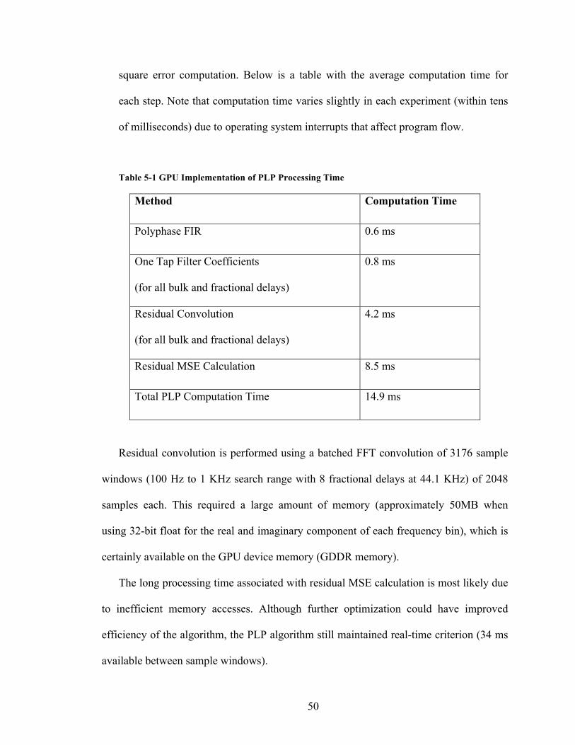
square error computation. Below is a table with the average computation time for
each step. Note that computation time varies slightly in each experiment (within tens
of milliseconds) due to operating system interrupts that affect program flow.
Table 5-1 GPU Implementation of PLP Processing Time
Method Computation Time
Polyphase FIR 0.6 ms
One Tap Filter Coefficients
(for all bulk and fractional delays)
0.8 ms
Residual Convolution
(for all bulk and fractional delays)
4.2 ms
Residual MSE Calculation 8.5 ms
Total PLP Computation Time 14.9 ms
Residual convolution is performed using a batched FFT convolution of 3176 sample
windows (100 Hz to 1 KHz search range with 8 fractional delays at 44.1 KHz) of 2048
samples each. This required a large amount of memory (approximately 50MB when
using 32-bit float for the real and imaginary component of each frequency bin), which is
certainly available on the GPU device memory (GDDR memory).
The long processing time associated with residual MSE calculation is most likely due
to inefficient memory accesses. Although further optimization could have improved
efficiency of the algorithm, the PLP algorithm still maintained real-time criterion (34 ms
available between sample windows).
51
5.2.2. AR Filter Implementation
The autoregressive filter was first implemented on the GPU. Preliminary results
showed that execution time took almost 20 ms. This was unexpected due to the small
amount of computation necessary. However, the bottleneck of the algorithm was in
numerous memory transfers between host and device memory, which was needed to
regulate the algorithm flow. This showed that this particular algorithm is ill suited for
GPU implementation. Therefore, a CPU implementation was done with considerable
speed improvement.
Since the autoregressive filter relied on the input signal autocorelation estimate, fast
computation of the autocorrelation lags was done on the GPU. The Wiener-Khinchin
theorem states that autocorrelation of a discrete sequence is the product of the sequence
and it’s complex conjugate in the frequency domain. This proved convenient since the
AR filter is computed after the PLP filter, which used FFT convolution for output signal
filtering.
Once the autocorrelation lags are available, the coefficients of the AR filter are
estimated using matrix inversion. GNU Scientific Library was used for matrix inversion.
The library provides optimized code for Linear Algebra computations on general-purpose
processors. Inversion of the 30x30 matrix took 0.6 ms on a 3.0 GHz Intel Core i3
development computer with 8 GB of RAM.
52
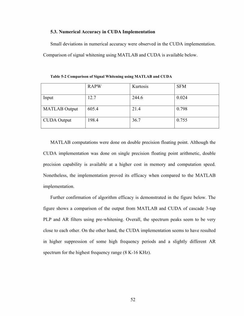
5.3. Numerical Accuracy in CUDA Implementation
Small deviations in numerical accuracy were observed in the CUDA implementation.
Comparison of signal whitening using MATLAB and CUDA is available below.
Table 5-2 Comparison of Signal Whitening using MATLAB and CUDA
RAPW Kurtosis SFM
Input 12.7 244.6 0.024
MATLAB Output 605.4 21.4 0.798
CUDA Output 198.4 36.7 0.755
MATLAB computations were done on double precision floating point. Although the
CUDA implementation was done on single precision floating point arithmetic, double
precision capability is available at a higher cost in memory and computation speed.
Nonetheless, the implementation proved its efficacy when compared to the MATLAB
implementation.
Further confirmation of algorithm efficacy is demonstrated in the figure below. The
figure shows a comparison of the output from MATLAB and CUDA of cascade 3-tap
PLP and AR filters using pre-whitening. Overall, the spectrum peaks seem to be very
close to each other. On the other hand, the CUDA implementation seems to have resulted
in higher suppression of some high frequency periods and a slightly different AR
spectrum for the highest frequency range (8 K-16 KHz).
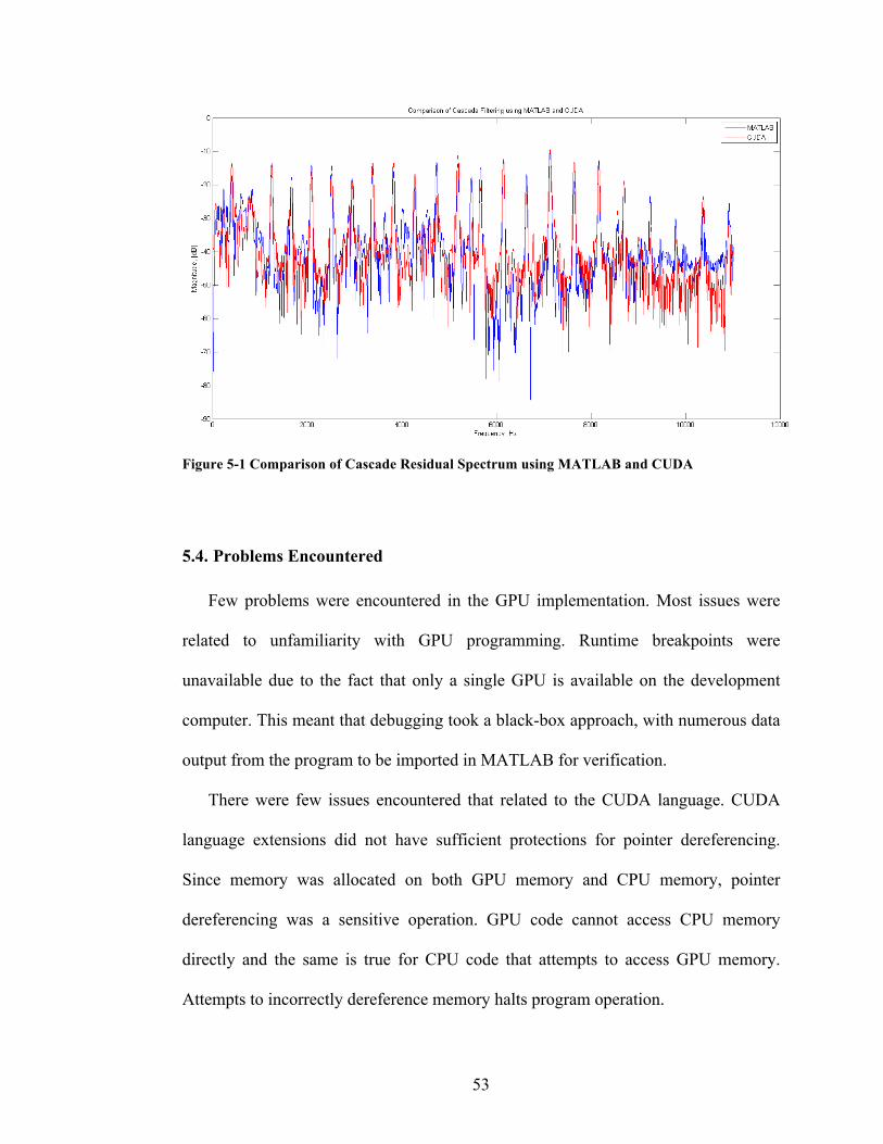
53
Figure 5-1 Comparison of Cascade Residual Spectrum using MATLAB and CUDA
5.4. Problems Encountered
Few problems were encountered in the GPU implementation. Most issues were
related to unfamiliarity with GPU programming. Runtime breakpoints were
unavailable due to the fact that only a single GPU is available on the development
computer. This meant that debugging took a black-box approach, with numerous data
output from the program to be imported in MATLAB for verification.
There were few issues encountered that related to the CUDA language. CUDA
language extensions did not have sufficient protections for pointer dereferencing.
Since memory was allocated on both GPU memory and CPU memory, pointer
dereferencing was a sensitive operation. GPU code cannot access CPU memory
directly and the same is true for CPU code that attempts to access GPU memory.
Attempts to incorrectly dereference memory halts program operation.
54
NVIDIA provides memory transfer functions that can copy data from host or
GPU memory given data size and data type. Therefore, prefixes were used on pointer
variables to denote where the data resides in order to prevent incorrect memory
dereferencing (e.g. D_PLPcoeff and H_PLPcoeff for pointers to data in device and
host memory, respectively).
Wide availability of NVIDIA GPUs made access to GPU programming trivial.
The algorithm was first prototyped on a 2008 model Apple Macbook Pro laptop.
Initial results showed that the PLP algorithm could execute in 80 ms. The bottleneck
of the algorithm was in device memory accesses. A low cost (approx. $150 USD)
video card was then sourced locally, which as stated above, has an 86.4 GB/sec
device memory bandwidth. Bandwidth tests on the Macbook Pro NVIDIA GPU
shows a memory bandwidth of only 1GB/sec.
When transferring data between host and GPU memory, pinned memory
allocation was necessary. Pinned memory refers to a memory area that is allocated on
the host, which the operating system cannot move to paged memory (which is located
on the hard drive). This is necessary in order to maximize throughput during memory
transfer between host and GPU memory. NVIDIA provides custom malloc () and
free () functions to provide this functionality.
55
Chapter 6 - Conclusions
6.1. Filters Performance
Results from the MATLAB simulation have shown that the AR filter is effective
at overall whitening of the signal spectrum. The dynamic range of the spectrum is
greatly reduced in all input cases.
On the other hand, the PLP filter is not very effective at suppressing higher
harmonics in recorded signals. This is due to the high number of harmonics present in
recorded signals. It seems that the harmonics are not precise integer number
harmonics, which is why the filter has not been able to suppress them when compared
to the synthesized test case.
Using the current configuration, comparable results are achieved on polyphonic
input signals. This is important due to the predominance of polyphony in music.
Real-time implementation of the AR filter is feasible for both DSP processors and
GPUs. However, the computational complexity of the PLP filter is too large for the
DSP processor. The GPU architecture proved to be well suited for the PLP filter
implementation.
Further improvements to audio signal whitening can be made to the pitch filter.
The computational power facilitated by the GPU can accommodate a combined
search and adaptive technique for suppressing the tonal components of the input
signal. Nonetheless, this work showed that the implementation of the AFC algorithm
is possible in real-time performance.
56
6.2. Development Cost
Overall, the GPU implementation is the most cost effective in terms of time and
hardware costs. In terms of hardware costs, the video card used in the implementation
is a gaming level GPU. The cost is, in a way, subsidized due to the volume of sales in
the PC gaming industry. Numerically, the video card was sourced locally for
approximately $150 USD. The PC itself was purchased for about $600 USD. The
CUDA SDK is provided at no cost.
The main drawback in using GPUs is in its large amount of power consumption.
The GPU alone is rated for a total of 150W of thermal power dissipation. Although the
CPU was not used extensively during runtime, its power dissipation should be
considered as well. It is worth mentioning that the Intel i architecture processors
includes a GPU. However, no SDK is currently available.
Development time took approximately three weeks. The author is an experienced
C/C++ programmer, but without any previous parallel programming experience.
Coding was done in a way that reflected the DSP algorithm, with very few
optimizations done for parallel programming.
6.3. Final Remarks
The availability of massively parallel architectures in GPUs provide a cost
effective development environment for suitable algorithms. This implementation of
whitening filters was made possible in real-time only through the use of GPUs.
Therefore, their further use in real-time DSP applications should be investigated.
57
References
[1] W. Gersch, “Spectral analysis of EEGʼs by autoregressive spectral decomposition of time series,” Mathematical Biosciences, vol. 7, 1970, pp. 205-222.
[2] E.A. Robinson, “Predictive decomposition of time series with application to seismic exploration,” Geophysics, vol. 32, 1967, p. 418.
[3] R.P. Ramachandran and P. Kabal, “Pitch prediction filters in speech coding,” IEEE Transactions on Acoustics Speech and Signal Processing, vol. 37, 1989, pp. 467-478.
[4] T. Van Waterschoot and M. Moonen, “Adaptive feedback cancellation for audio applications,” Signal Processing, vol. 89, 2009, pp. 2185-2201.
[5] T. Van Waterschoot and M. Moonen, “Fifty Years of Acoustic Feedback Control: State of the Art and Future Challenges,” Proceedings of the IEEE, vol. PP, 2010, pp. 1-40.
[6] T.V. Waterschoot and M. Moonen, “ASSESSING THE ACOUSTIC FEEDBACK CONTROL PERFORMANCE OF ADAPTIVE FEEDBACK CANCELLATION IN SOUND REINFORCEMENT SYSTEMS Toon van Waterschoot and Marc Moonen,” Signal Processing, 2009, pp. 1997-2001.
[7] J. Makhoul, “Linear prediction: A tutorial review,” Proceedings of the IEEE, vol. 63, 1975, pp. 561-580.
[8] Y. Qian, G. Chahine, and P. Kabal, “Pseudo-multi-tap pitch filters in a low bit-rate CELP speech coder,” Speech Communication, vol. 14, 1994, pp. 339-358.
[9] G.U. Yule, “On a Method of Investigating Periodicities in Disturbed Series, with Special Reference to Wolferʼs Sunspot Numbers,” Phill Trans, vol. 226, 1927, pp. 267-298.
[10] G. Zelniker and F.J. Taylor, Advanced Digital Signal Processing: Theory and Applications (Electrical Engineering & Electronics), CRC Press, 1993.
[11] M. Dehoon, T. Vanderhagen, H. Schoonewelle, and H. Van Dam, “Why Yule-Walker should not be used for autoregressive modelling,” Annals of Nuclear Energy, vol. 23, 1996, pp. 1219-1228.
58
[12] T. Van Waterschoot and M. Moonen, “Comparison of Linear Prediction Models for Audio Signals,” EURASIP Journal on Audio Speech and Music Processing, vol. 2008, 2008, pp. 1-25.
[13] T.I. Laakso, V. Välimäki, M. Karjalainen, and U.K. Laine, “Splitting the Unit Delay---Tools for Fractional Delay Filter Design,” IEEE Signal Processing Magazine, vol. 13, 1996, pp. 30-60.
[14] J. Makhoul, “Linear prediction: A tutorial review,” Proceedings of the IEEE, vol. 63, 1975, pp. 561-580.
[15] K.P. Balanda and H.L. MacGillivray, “Kurtosis: A Critical Review,” American Statistician, vol. 42, 1988, p. 111.
[16] A. Gray and J. Markel, “A Spectral-Flatness Measure for Studying the Autocorrelation Method of Linear Predication of Speech Analysis,” IEEE Transactions on Acoustics Speech and Signal Processing, vol. 22, 1974, pp. 207-217.
[17] “Piano key frequencies - Wikipedia, the free encyclopedia.” [online] http://en.wikipedia.org/wiki/Piano_key_frequencies (accessed: June 20, 2011).
[18] “eins - Wiktionary.” [online] http://en.wiktionary.org/wiki/eins (accessed: June 20, 2011).
[19] K. Karplus and A. Strong, “Digital synthesis of plucked-string and drum timbres,” Computer Music Journal, vol. 7, 1983, pp. 43-55.
[20] C. Collomb, “Linear Prediction and the Levinson-Durbin algorithm,” 2009, pp. 1-7.
[21] G.-J. Inversion, “Gauss-Jordan Inversion of a Matrix,” October, 1998, pp. 1-4.
[22] J. Xu, A. Ariyaeeinia, and R. Sotudeh, “Migrate Levinson-Durbin based Linear Predictive Coding algorithm into FPGAS,” 2005 12th IEEE International Conference on Electronics, Circuits and Systems, Dec. 2005, pp. 1-4.
[23] L. Savioja, V. Valimaki, and J. Smith, “Audio Signal Processing Using Graphics Processing Units,” submitted to Journal of the Audio Engineering Society, 2010, pp. 3-19.
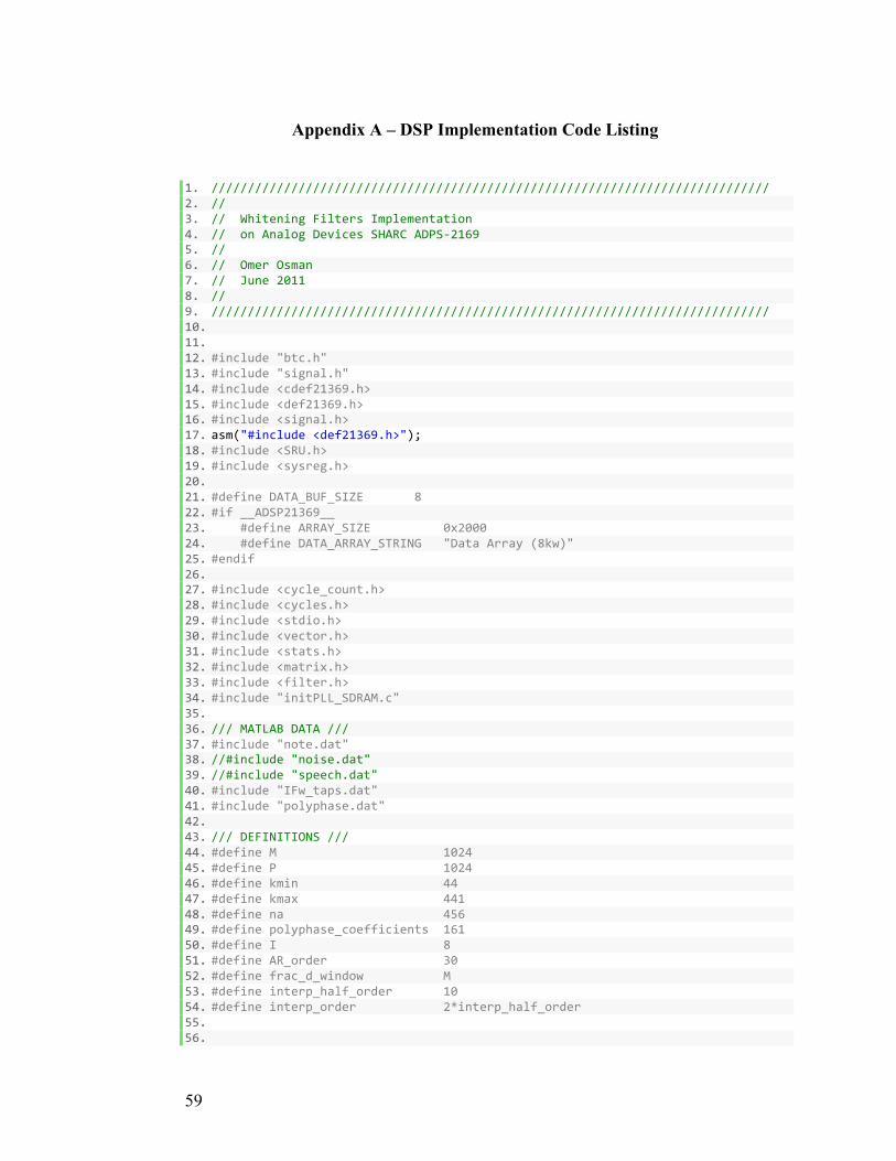
59
Appendix A – DSP Implementation Code Listing
1. ///////////////////////////////////////////////////////////////////////////// 2. // 3. // Whitening Filters Implementation 4. // on Analog Devices SHARC ADPS-‐2169 5. // 6. // Omer Osman 7. // June 2011 8. // 9. ///////////////////////////////////////////////////////////////////////////// 10. 11. 12. #include "btc.h" 13. #include "signal.h" 14. #include <cdef21369.h> 15. #include <def21369.h> 16. #include <signal.h> 17. asm("#include <def21369.h>"); 18. #include <SRU.h> 19. #include <sysreg.h> 20. 21. #define DATA_BUF_SIZE 8 22. #if __ADSP21369__ 23. #define ARRAY_SIZE 0x2000 24. #define DATA_ARRAY_STRING "Data Array (8kw)" 25. #endif 26. 27. #include <cycle_count.h> 28. #include <cycles.h> 29. #include <stdio.h> 30. #include <vector.h> 31. #include <stats.h> 32. #include <matrix.h> 33. #include <filter.h> 34. #include "initPLL_SDRAM.c" 35. 36. /// MATLAB DATA /// 37. #include "note.dat" 38. //#include "noise.dat" 39. //#include "speech.dat" 40. #include "IFw_taps.dat" 41. #include "polyphase.dat" 42. 43. /// DEFINITIONS /// 44. #define M 1024 45. #define P 1024 46. #define kmin 44 47. #define kmax 441 48. #define na 456 49. #define polyphase_coefficients 161 50. #define I 8 51. #define AR_order 30 52. #define frac_d_window M 53. #define interp_half_order 10 54. #define interp_order 2*interp_half_order 55. 56.
60
57. /// extern GLOBAL VARIABLES /// 58. extern void InitPLL_SDRAM(void); 59. extern const float pm note [M]; 60. //extern const float dm noise [M]; 61. //extern const float dm speech [M]; 62. extern float pm polyphase_coeff [161]; 63. 64. 65. 66. //////////////////////////// 67. // Variable Definitions 68. //////////////////////////// 69. int timerCounter = 0; 70. int dataVal = 0x11223344; 71. int dataBuf[DATA_BUF_SIZE] = {0x11223344,0x55667788,0x99aabbcc,0xddeeff00, 72. 0x55555555,0x66666666,0x77777777,0x88888888}; 73. int array1[ARRAY_SIZE]; 74. 75. float 76. ARcoeff [AR_order+1]; 77. float 78. PLPcoeff [na+1]; 79. float 80. fracDelay[M]; 81. 82. float 83. fir_input[(frac_d_window+10)*I]; 84. float 85. fir_output[(frac_d_window+10)*I]; 86. 87. 88. // PLP 89. float 90. bestMSE[3]; 91. float pm 92. prediction_error [kmax+M+interp_half_order+1]; 93. float 94. response [kmax+interp_half_order+2]; 95. float pm 96. responseR [kmax+interp_half_order+2]; 97. float pm 98. PLPiR [kmax+interp_half_order+2]; 99. 100. 101. float 102. x_0 [M-‐kmin]; 103. float 104. x_Mmin [M-‐kmin]; 105. float 106. x_M [M-‐kmin]; 107. float 108. x_Mplus [M-‐kmin]; 109. float 110. a_0[3]; 111. float 112. a_M[3]; 113. float 114. taps[3]; 115. 116. float 117. delta;
61
118. float 119. Rxx [AR_order+1]; 120. float 121. kappa; 122. float 123. kappa2; 124. float 125. sigma2; 126. double 127. status [2]; 128. 129. //////////////////////// 130. // Function Prototypes 131. //////////////////////// 132. void initInterrupts(void); 133. void initTimer(void); 134. 135. void GPTimer0_isr(int signal); 136. 137. void findARcoeff (const float* X, float* ARcoeff); 138. void findPLPcoeff (const float[], float* PLPcoeff); 139. void frac_delay (const float* X); 140. void one_tap_polyphasePLP (const float* X); 141. void three_tap_polyphasePLP (const float* X); 142. 143. 144. // ASSEMBLY ROUTINE FOR RECIPROCAL DIVISION // 145. // FROM SHARC 21369 PROGRAMMING MANUAL // 146. // CAN BE EXPANDED FOR HIGHER PRECISION // 147. // REF-‐ NEWTON-‐RAPHSON METHOD // 148. /* 149. .global _fp_division; 150. _fp_division: 151. F0=%1;" // numerator 152. F12=%2;" // denominator 153. F11=%3;" // 2.0 154. F0=RECIPS F12, F7=F0;" // {Get 8 bit seed R0=1/D} 155. F12=F0*F12;" // {D' = D*R0} 156. F7=F0*F7, F0=F11-‐F12;" // {F0=R1=2-‐D', F7=N*R0} 157. F12=F0*F12;" // {F12=D'-‐D'*R1} 158. F7=F0*F7, F0=F11-‐F12;" // {F7=N*R0*R1, F0=R2=2-‐D'} 159. F12=F0*F12;" // {F12=D'=D'*R2} 160. RTS(DB); 161. F7=F0*F7, F0=F11-‐F12;" // {F7=N*R0*R1*R2, F0=R3=2-‐D'} 162. F0=F0*F7; 163. %0=F0*F7;" // {F7=N*R0*R1*R2*R3} 164. "=F" (sigma2) 165. : "F" (x), "F" (y), "F" (z) 166. : "F0", "F12", "F11", "F7"); 167. */ 168. 169. //////////////////// 170. // BACKGROUND TELEMETRY CHANNEL Definitions 171. //////////////////// 172. BTC_MAP_BEGIN 173. // Channel Name, Starting Address, Length 174. BTC_MAP_ENTRY("Timer Interrupt Counter", (long)&timerCounter, sizeof(tim
erCounter)) 175. BTC_MAP_ENTRY("Constant Data Value", (long)&dataVal, sizeof(dat
aVal))
62
176. BTC_MAP_ENTRY("Constant Data Buffer", (long)dataBuf, sizeof(dataBuf))
177. BTC_MAP_ENTRY(DATA_ARRAY_STRING, (long)array1, sizeof(array1))
178. BTC_MAP_ENTRY("Delta", (long)&delta, sizeof(delta))
179. BTC_MAP_ENTRY("Sigma2", (long)&sigma2, sizeof(sigma2))
180. BTC_MAP_ENTRY("Rxx", (long)Rxx, sizeof(Rxx))
181. BTC_MAP_ENTRY("kappa", (long)&kappa, sizeof(kappa))
182. BTC_MAP_ENTRY("kappa2", (long)&kappa2, sizeof(kappa2))
183. BTC_MAP_ENTRY("ARCoefficients", (long)ARcoeff, sizeof(ARcoeff))
184. BTC_MAP_ENTRY("FracDelay", (long)fracDelay, sizeof(fracDelay))
185. BTC_MAP_ENTRY("ASTATx ASTATy", (long)status, sizeof(status))
186. BTC_MAP_END 187. 188. /////////////////// 189. // Main Program 190. /////////////////// 191. int main() 192. { 193. InitPLL_SDRAM(); 194. 195. //sysreg_bit_clr(sysreg_MMASK, PEYEN); // ENABLE SECOND ALU 196. //sysreg_bit_set(sysreg_MODE1, PEYEN); // set Processor Element Y (
SIMD) enable 197. //sysreg_bit_clr(sysreg_MODE1, RND32); // set IEEE-‐754 32-‐
bit Floating Point 198. sysreg_bit_set(sysreg_MODE1, CBUFEN); // set hardware circular buffe
r enable 199. //sysreg_bit_clr(sysreg_MODE1, TRUNC); // set truncation mode to ne
arest 200. ///sysreg_bit_set(sysreg_MODE1, NESTM); // set nested multiple inte
rrupts enable 201. //sysreg_bit_set(sysreg_MODE1, IRPTEN); // set interrupt enable 202. 203. 204. int addr, len; 205. addr = BTC_CHANNEL_ADDR(0); 206. len = BTC_CHANNEL_LEN(0); 207. 208. for(int i = 0; i < ARRAY_SIZE; ++i) 209. { 210. array1[i] = i; 211. } 212. 213. // initialize 214. btc_init(); 215. 216. initTimer(); 217. interrupt(SIG_EMUL, btc_isr); 218. 219. cycle_t 220. start_count; 221. cycle_t
63
222. final_count; 223. 224. // profiling functionality // 225. //START_CYCLE_COUNT(start_count); 226. 227. findARcoeff (speech, ARcoeff); 228. 229. //STOP_CYCLE_COUNT(final_count,start_count); 230. //PRINT_CYCLES("Number of cycles for AR Filter: ",final_count); 231. 232. findPLPcoeff (note, PLPcoeff); 233. 234. initInterrupts(); 235. 236. //while(1); 237. 238. } 239. 240. 241. void initInterrupts() 242. { 243. interrupt(SIG_P2, GPTimer0_isr); 244. } 245. 246. 247. void initTimer() 248. { 249. 250. *pTM0CTL = TIMODEPWM | PRDCNT | IRQEN; // configure the timer 251. *pTM0PRD = 0x00800000; // timer period 252. *pTM0W = 1; // timer width 253. *pTMSTAT = BIT_8; // enable the timer 254. } 255. 256. 257. void GPTimer0_isr(int signal) 258. { 259. // clear timer interrupt status 260. *pTMSTAT = TIM0IRQ; 261. 262. ++timerCounter; // count number of timer interrupts 263. array1[0] = timerCounter; // reflect count in first location of ar
ray1 264. 265. // toggle LED1 on the EZ-‐Kit 266. asm("bit tgl flags FLG4;"); //light LED 1 267. 268. } 269. 270. // AR coefficient estimation using levinson durbin 271. void findARcoeff (const float* X, float* Coeffs) 272. { 273. 274. // moved as global vars 275. // float 276. // Rxx [AR_order+1]; 277. // float 278. // alpha [AR_order]; 279. // float 280. // delta; 281. // float
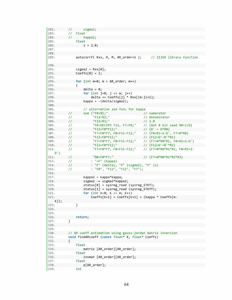
64
282. // sigma2; 283. // float 284. // kappa2; 285. float 286. z = 2.0; 287. 288. 289. autocorrf( Rxx, X, M, AR_order+1 ); // 21369 library function
290. 291. sigma2 = Rxx[0]; 292. Coeffs[0] = 1; 293. 294. for (int m=0; m < AR_order; m++) 295. { 296. delta = 0; 297. for (int j=0; j <= m; j++) 298. delta += Coeffs[j] * Rxx[(m-‐j)+1]; 299. kappa = -‐(delta/sigma2); 300. 301. // alternative asm func for kappa 302. // asm ("F0=%1;" // numerator 303. // "F12=%2;" // denominator 304. // "F11=%3;" // 2.0 305. // "F0=RECIPS F12, F7=F0;" // {Get 8 bit seed R0=1/D} 306. // "F12=F0*F12;" // {D' = D*R0} 307. // "F7=F0*F7, F0=F11-‐F12;" // {F0=R1=2-‐D', F7=N*R0} 308. // "F12=F0*F12;" // {F12=D'-‐D'*R1} 309. // "F7=F0*F7, F0=F11-‐F12;" // {F7=N*R0*R1, F0=R2=2-‐D'} 310. // "F12=F0*F12;" // {F12=D'=D'*R2} 311. // "F7=F0*F7, F0=F11-‐F12;" // {F7=N*R0*R1*R2, F0=R3=2-‐
D'} 312. // "%0=F0*F7;" // {F7=N*R0*R1*R2*R3} 313. // : "=F" (kappa) 314. // : "F" (delta), "F" (sigma2), "F" (z) 315. // : "F0", "F12", "F11", "F7"); 316. 317. kappa2 = kappa*kappa; 318. sigma2 -‐= sigma2*kappa2; 319. status[0] = sysreg_read (sysreg_STKY); 320. status[1] = sysreg_read (sysreg_STKYY); 321. for (int k=0; k <= m; k++) 322. Coeffs[k+1] = Coeffs[k+1] + (kappa * Coeffs[m-‐
k]); 323. } 324. 325. 326. return; 327. } 328. 329. 330. // AR coeff estimation using gauss-‐jordan matrix inversion 331. void findARcoeff (const float* X, float* Coeffs) 332. { 333. float 334. matrix [AR_order][AR_order]; 335. float 336. invmat [AR_order][AR_order]; 337. float 338. p[AR_order]; 339. int
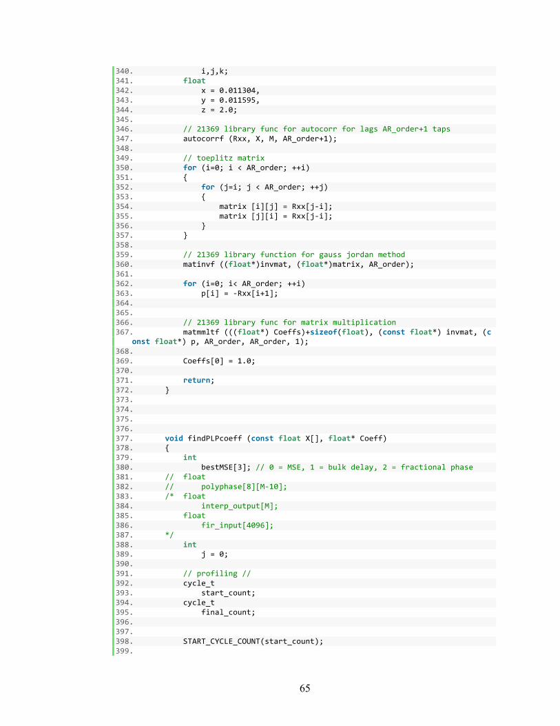
65
340. i,j,k; 341. float 342. x = 0.011304, 343. y = 0.011595, 344. z = 2.0; 345. 346. // 21369 library func for autocorr for lags AR_order+1 taps 347. autocorrf (Rxx, X, M, AR_order+1); 348. 349. // toeplitz matrix 350. for (i=0; i < AR_order; ++i) 351. { 352. for (j=i; j < AR_order; ++j) 353. { 354. matrix [i][j] = Rxx[j-‐i]; 355. matrix [j][i] = Rxx[j-‐i]; 356. } 357. } 358. 359. // 21369 library function for gauss jordan method 360. matinvf ((float*)invmat, (float*)matrix, AR_order); 361. 362. for (i=0; i< AR_order; ++i) 363. p[i] = -‐Rxx[i+1]; 364. 365. 366. // 21369 library func for matrix multiplication 367. matmmltf (((float*) Coeffs)+sizeof(float), (const float*) invmat, (c
onst float*) p, AR_order, AR_order, 1); 368. 369. Coeffs[0] = 1.0; 370. 371. return; 372. } 373. 374. 375. 376. 377. void findPLPcoeff (const float X[], float* Coeff) 378. { 379. int 380. bestMSE[3]; // 0 = MSE, 1 = bulk delay, 2 = fractional phase 381. // float 382. // polyphase[8][M-‐10]; 383. /* float 384. interp_output[M]; 385. float 386. fir_input[4096]; 387. */ 388. int 389. j = 0; 390. 391. // profiling // 392. cycle_t 393. start_count; 394. cycle_t 395. final_count; 396. 397. 398. START_CYCLE_COUNT(start_count); 399.
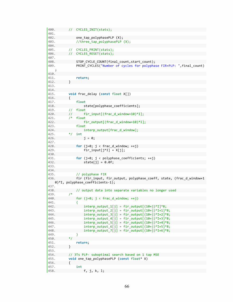
66
400. // CYCLES_INIT(stats); 401. 402. one_tap_polyphasePLP (X); 403. //three_tap_polyphasePLP (X); 404. 405. // CYCLES_PRINT(stats); 406. // CYCLES_RESET(stats); 407. 408. STOP_CYCLE_COUNT(final_count,start_count); 409. PRINT_CYCLES("Number of cycles for polyphase FIR+PLP: ",final_count)
; 410. 411. return; 412. } 413. 414. 415. void frac_delay (const float X[]) 416. { 417. float 418. state[polyphase_coefficients]; 419. // float 420. // fir_input[(frac_d_window+10)*I]; 421. /* float 422. fir_output[(frac_d_window+10)*I]; 423. float 424. interp_output[frac_d_window]; 425. */ int 426. j = 0; 427. 428. for (j=0; j < frac_d_window; ++j) 429. fir_input[j*I] = X[j]; 430. 431. for (j=0; j < polyphase_coefficients; ++j) 432. state[j] = 0.0f; 433. 434. 435. // polyphase FIR 436. fir (fir_input, fir_output, polyphase_coeff, state, (frac_d_window+1
0)*I, polyphase_coefficients-‐1); 437. 438. // output data into separate variables no longer used 439. /* 440. for (j=0; j < frac_d_window; ++j) 441. { 442. interp_output_1[j] = fir_output[(10+j)*I]*8; 443. interp_output_2[j] = fir_output[(10+j)*I+1]*8; 444. interp_output_3[j] = fir_output[(10+j)*I+2]*8; 445. interp_output_4[j] = fir_output[(10+j)*I+3]*8; 446. interp_output_5[j] = fir_output[(10+j)*I+4]*8; 447. interp_output_6[j] = fir_output[(10+j)*I+5]*8; 448. interp_output_7[j] = fir_output[(10+j)*I+6]*8; 449. } 450. */ 451. return; 452. } 453. 454. // 3Ts PLP-‐ suboptimal search based on 1 tap MSE 455. void one_tap_polyphasePLP (const float* X) 456. { 457. int 458. f, j, k, l;
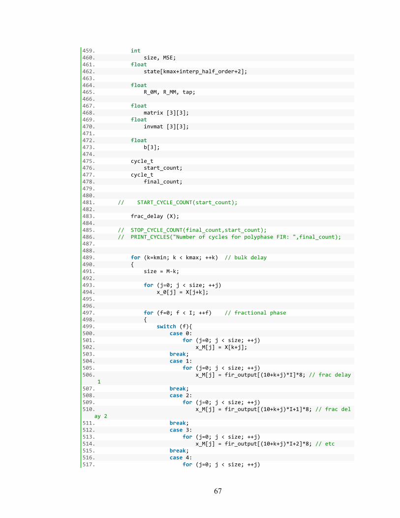
67
459. int 460. size, MSE; 461. float 462. state[kmax+interp_half_order+2]; 463. 464. float 465. R_0M, R_MM, tap; 466. 467. float 468. matrix [3][3]; 469. float 470. invmat [3][3]; 471. 472. float 473. b[3]; 474. 475. cycle_t 476. start_count; 477. cycle_t 478. final_count; 479. 480. 481. // START_CYCLE_COUNT(start_count); 482. 483. frac_delay (X); 484. 485. // STOP_CYCLE_COUNT(final_count,start_count); 486. // PRINT_CYCLES("Number of cycles for polyphase FIR: ",final_count); 487. 488. 489. for (k=kmin; k < kmax; ++k) // bulk delay 490. { 491. size = M-‐k; 492. 493. for (j=0; j < size; ++j) 494. x_0[j] = X[j+k]; 495. 496. 497. for (f=0; f < I; ++f) // fractional phase 498. { 499. switch (f){ 500. case 0: 501. for (j=0; j < size; ++j) 502. x_M[j] = X[k+j]; 503. break; 504. case 1: 505. for (j=0; j < size; ++j) 506. x_M[j] = fir_output[(10+k+j)*I]*8; // frac delay
1 507. break; 508. case 2: 509. for (j=0; j < size; ++j) 510. x_M[j] = fir_output[(10+k+j)*I+1]*8; // frac del
ay 2 511. break; 512. case 3: 513. for (j=0; j < size; ++j) 514. x_M[j] = fir_output[(10+k+j)*I+2]*8; // etc 515. break; 516. case 4: 517. for (j=0; j < size; ++j)
68
518. x_M[j] = fir_output[(10+k+j)*I+3]*8; 519. break; 520. case 5: 521. for (j=0; j < size; ++j) 522. x_M[j] = fir_output[(10+k+j)*I+4]*8; 523. break;
524. case 6: 525. for (j=0; j < size; ++j) 526. x_M[j] = fir_output[(10+k+j)*I+5]*8; 527. break; 528. case 7: 529. for (j=0; j < size; ++j) 530. x_M[j] = fir_output[(10+k+j)*I+6]*8; 531. break; 532. } 533. 534. // one tap plp calculation 535. R_0M = vecdotf (x_0, x_M, size); 536. R_MM = vecdotf (x_M, x_M, size); 537. 538. tap = R_0M/R_MM; 539. 540. for (j=0; j < k+interp_order+2; ++j) 541. response[j] = 0.0; 542. 543. response [0] = 1; 544. for (j=k-‐
interp_half_order+1; j < k+interp_half_order+1; ++j) 545. response[j] = -‐tap*IFw_taps[f][j-‐k+interp_half_order]; 546. 547. for (j=0; j < k+interp_order+1; ++j) 548. responseR[j] = response[(k+interp_order)-‐j]; 549. 550. for (j=0; j < kmax+interp_half_order+2; ++j) 551. state[j] = 0.0f; 552. 553. // MOST time consumption is in this line of code 554. START_CYCLE_COUNT(start_count); 555. fir (X, prediction_error, responseR, state, M, k+interp_orde
r+1); 556. STOP_CYCLE_COUNT(final_count,start_count); 557. PRINT_CYCLES("Number of cycles : ",final_count);
558. 559. // MSE calc 560. MSE = vecdotf(prediction_error, prediction_error, M); 561. 562. if (MSE <= 0) 563. MSE = 10000; // null condition 564. 565. if (bestMSE[0] > MSE || bestMSE[2] == 0) 566. { 567. bestMSE[0] = MSE; 568. bestMSE[1] = k; 569. bestMSE[2] = f; 570. } 571. } 572. } 573. 574.
69
575. // 3 tap coefficients calc based on best 1-‐tap plp 576. k = bestMSE[1]; 577. f = bestMSE[2]; 578. size = M-‐k; 579. 580. for (j=0; j < size; ++j) 581. x_0[j] = X[j+k+1]; 582. 583. 584. for (j=0; j < size; ++j) 585. { 586. x_Mmin[j] = fir_output[(10+k+j-‐1)*I+f-‐1]*8; 587. x_M[j] = fir_output[(10+k+j)*I+f-‐1]*8; 588. x_Mplus[j] = fir_output[(10+k+j+1)*I+f-‐1]*8; 589. } 590. 591. a_0[0] = vecdotf(x_0, x_Mmin, size); 592. a_0[1] = vecdotf (x_0, x_M, size); 593. a_0[2] = vecdotf (x_0, x_Mplus, size); 594. a_M[0] = vecdotf (x_Mmin, x_Mmin, size); 595. a_M[1] = vecdotf (x_Mmin, x_M, size); 596. a_M[2] = vecdotf(x_Mmin, x_Mplus, size); 597. 598. 599. for (l=0; l < 3; ++l) 600. { 601. for (j=l; j < 3; ++j) 602. { 603. matrix [l][j] = a_M[j-‐l]; 604. matrix [j][l] = a_M[j-‐l]; 605. } 606. } 607. 608. b[0] = a_0[0]; 609. b[1] = a_0[1]; 610. b[2] = a_0[2]; 611. 612. matinvf ((float*)invmat, (float*)matrix, 3); 613. 614. matmmltf ((float*)taps, (const float*)invmat, (const float*)b, 3, 3,
1); 615. 616. for (j=0; j < k+interp_order+2; ++j) 617. PLPiR[j] = 0.0; 618. 619. PLPiR[0] = 1; 620. for (j=k-‐
interp_half_order; j < k+interp_half_order; ++j) // first tap 621. PLPiR[j] = -‐taps[0]*IFw_taps[f][j-‐k+interp_half_order]; 622. for (j=k-‐interp_half_order; j < k+interp_half_order; ++j) // 2nd 623. PLPiR[j+1] -‐= taps[1]*IFw_taps[f][j-‐k+interp_half_order]; 624. for (j=k-‐interp_half_order; j < k+interp_half_order; ++j) // 3rd 625. PLPiR[j+2] -‐= taps[2]*IFw_taps[f][j-‐
k+interp_half_order]; 626. 627. for (j=0; j < k+interp_order+1; ++j) 628. responseR[j] = PLPiR[(k+interp_order)-‐j]; 629. 630. for (j=0; j < kmax+interp_half_order+2; ++j) 631. state[j] = 0.0f; 632.
70
633. fir (X, prediction_error, responseR, state, M, k+interp_order+1); 634. 635. sigma2 = vecdotf(prediction_error, prediction_error, M); 636. 637. return; 638. } 639. 640. 641. // exhaustive search PLP 642. void three_tap_polyphasePLP (const float* X) 643. { 644. 645. int 646. f, j, k, l; 647. int 648. size, MSE; 649. float 650. state[kmax+interp_half_order+2]; 651. 652. float 653. R_0M, R_MM, tap; 654. 655. float 656. matrix [3][3]; 657. float 658. invmat [3][3]; 659. 660. float 661. b[3]; 662. 663. frac_delay (X); 664. 665. for (k=kmin; k < kmax; ++k) // bulk delay 666. { 667. size = M-‐k; 668. 669. for (j=0; j < size; ++j) 670. x_0[j] = X[j+k]; 671. 672. 673. for (f=0; f < I; ++f) // fractional phase 674. { 675. switch (f){ 676. case 0: 677. for (j=0; j < size; ++j) 678. x_M[j] = X[k+j]; 679. break; 680. case 1: 681. for (j=0; j < size; ++j) 682. x_M[j] = fir_output[(10+k+j)*I]*8; // frac delay
1 683. break; 684. case 2: 685. for (j=0; j < size; ++j) 686. x_M[j] = fir_output[(10+k+j)*I+1]*8; 687. break; 688. case 3: 689. for (j=0; j < size; ++j) 690. x_M[j] = fir_output[(10+k+j)*I+2]*8; 691. break; 692. case 4:
71
693. for (j=0; j < size; ++j) 694. x_M[j] = fir_output[(10+k+j)*I+3]*8; 695. break; 696. case 5: 697. for (j=0; j < size; ++j) 698. x_M[j] = fir_output[(10+k+j)*I+4]*8; 699. break;
700. case 6: 701. for (j=0; j < size; ++j) 702. x_M[j] = fir_output[(10+k+j)*I+5]*8; 703. break; 704. case 7: 705. for (j=0; j < size; ++j) 706. x_M[j] = fir_output[(10+k+j)*I+6]*8; 707. break; 708. } 709. 710. R_0M = vecdotf (x_0, x_M, size); 711. R_MM = vecdotf (x_M, x_M, size); 712. 713. tap = R_0M/R_MM; 714. 715. for (j=0; j < k+interp_order+2; ++j) 716. response[j] = 0.0; 717. 718. response [0] = 1; 719. for (j=k-‐
interp_half_order+1; j < k+interp_half_order+1; ++j) 720. response[j] = -‐tap*IFw_taps[f][j-‐k+interp_half_order]; 721. 722. for (j=0; j < k+interp_order+1; ++j) 723. responseR[j] = response[(k+interp_order)-‐j]; 724. 725. for (j=0; j < kmax+interp_half_order+2; ++j) 726. state[j] = 0.0f; 727. 728. fir (X, prediction_error, responseR, state, M, k+interp_orde
r+1); 729. 730. MSE = vecdotf(prediction_error, prediction_error, M); 731. 732. // 3 tap filter response 733. size = M-‐k; 734. 735. for (j=0; j < size; ++j) 736. x_0[j] = X[j+k+1]; 737. 738. 739. for (j=0; j < size; ++j) 740. { 741. x_Mmin[j] = fir_output[(10+k+j-‐1)*I+f-‐1]*8; 742. x_M[j] = fir_output[(10+k+j)*I+f-‐1]*8; 743. x_Mplus[j] = fir_output[(10+k+j+1)*I+f-‐
1]*8; 744. } 745. 746. a_0[0] = vecdotf(x_0, x_Mmin, size); 747. a_0[1] = vecdotf (x_0, x_M, size); 748. a_0[2] = vecdotf (x_0, x_Mplus, size); 749. a_M[0] = vecdotf (x_Mmin, x_Mmin, size);
72
750. a_M[1] = vecdotf (x_Mmin, x_M, size); 751. a_M[2] = vecdotf(x_Mmin, x_Mplus, size); 752. 753. 754. for (l=0; l < 3; ++l) 755. { 756. for (j=l; j < 3; ++j) 757. { 758. matrix [l][j] = a_M[j-‐l]; 759. matrix [j][l] = a_M[j-‐l]; 760. } 761. } 762. 763. b[0] = a_0[0]; 764. b[1] = a_0[1]; 765. b[2] = a_0[2]; 766. 767. matinvf ((float*)invmat, (float*)matrix, 3); 768. 769. matmmltf ((float*)taps, (const float*)invmat, (const float*)
b, 3, 3, 1); 770. 771. for (j=0; j < k+interp_order+2; ++j) 772. PLPiR[j] = 0.0; 773. 774. PLPiR[0] = 1; 775. for (j=k-‐
interp_half_order; j < k+interp_half_order; ++j) // first tap 776. PLPiR[j] = -‐taps[0]*IFw_taps[f][j-‐
k+interp_half_order]; 777. for (j=k-‐
interp_half_order; j < k+interp_half_order; ++j) // 2nd 778. PLPiR[j+1] -‐= taps[1]*IFw_taps[f][j-‐
k+interp_half_order]; 779. for (j=k-‐
interp_half_order; j < k+interp_half_order; ++j) // 3rd 780. PLPiR[j+2] -‐= taps[2]*IFw_taps[f][j-‐
k+interp_half_order]; 781. 782. for (j=0; j < k+interp_order+1; ++j) 783. responseR[j] = PLPiR[(k+interp_order)-‐j]; 784. 785. for (j=0; j < kmax+interp_half_order+2; ++j) 786. state[j] = 0.0f; 787. 788. fir (X, prediction_error, responseR, state, M, k+interp_orde
r+1); 789. 790. MSE = vecdotf(prediction_error, prediction_error, M); 791. 792. 793. if (MSE <= 0) 794. MSE = 10000; 795. 796. if (bestMSE[0] > MSE || bestMSE[2] == 0) 797. { 798. bestMSE[0] = MSE; 799. bestMSE[1] = k; 800. bestMSE[2] = f; 801. } 802. }
73
803. } 804. 805. // 3 tap filter response 806. k = bestMSE[1]; 807. f = bestMSE[2]; 808. size = M-‐k; 809. 810. for (j=0; j < size; ++j) 811. x_0[j] = X[j+k+1]; 812. 813. 814. for (j=0; j < size; ++j) 815. { 816. x_Mmin[j] = fir_output[(10+k+j-‐1)*I+f-‐1]*8; 817. x_M[j] = fir_output[(10+k+j)*I+f-‐1]*8; 818. x_Mplus[j] = fir_output[(10+k+j+1)*I+f-‐1]*8; 819. } 820. 821. a_0[0] = vecdotf(x_0, x_Mmin, size); 822. a_0[1] = vecdotf (x_0, x_M, size); 823. a_0[2] = vecdotf (x_0, x_Mplus, size); 824. a_M[0] = vecdotf (x_Mmin, x_Mmin, size); 825. a_M[1] = vecdotf (x_Mmin, x_M, size); 826. a_M[2] = vecdotf(x_Mmin, x_Mplus, size); 827. 828. 829. for (l=0; l < 3; ++l) 830. { 831. for (j=l; j < 3; ++j) 832. { 833. matrix [l][j] = a_M[j-‐l]; 834. matrix [j][l] = a_M[j-‐l]; 835. } 836. } 837. 838. b[0] = a_0[0]; 839. b[1] = a_0[1]; 840. b[2] = a_0[2]; 841. 842. matinvf ((float*)invmat, (float*)matrix, 3); 843. 844. matmmltf ((float*)taps, (const float*)invmat, (const float*)b, 3, 3,
1); 845. 846. for (j=0; j < k+interp_order+2; ++j) 847. PLPiR[j] = 0.0; 848. 849. PLPiR[0] = 1; 850. for (j=k-‐
interp_half_order; j < k+interp_half_order; ++j) // first tap 851. PLPiR[j] = -‐taps[0]*IFw_taps[f][j-‐k+interp_half_order]; 852. for (j=k-‐interp_half_order; j < k+interp_half_order; ++j) // 2nd 853. PLPiR[j+1] -‐= taps[1]*IFw_taps[f][j-‐k+interp_half_order]; 854. for (j=k-‐interp_half_order; j < k+interp_half_order; ++j) // 3rd 855. PLPiR[j+2] -‐= taps[2]*IFw_taps[f][j-‐
k+interp_half_order]; 856. 857. 858. return; 859. }
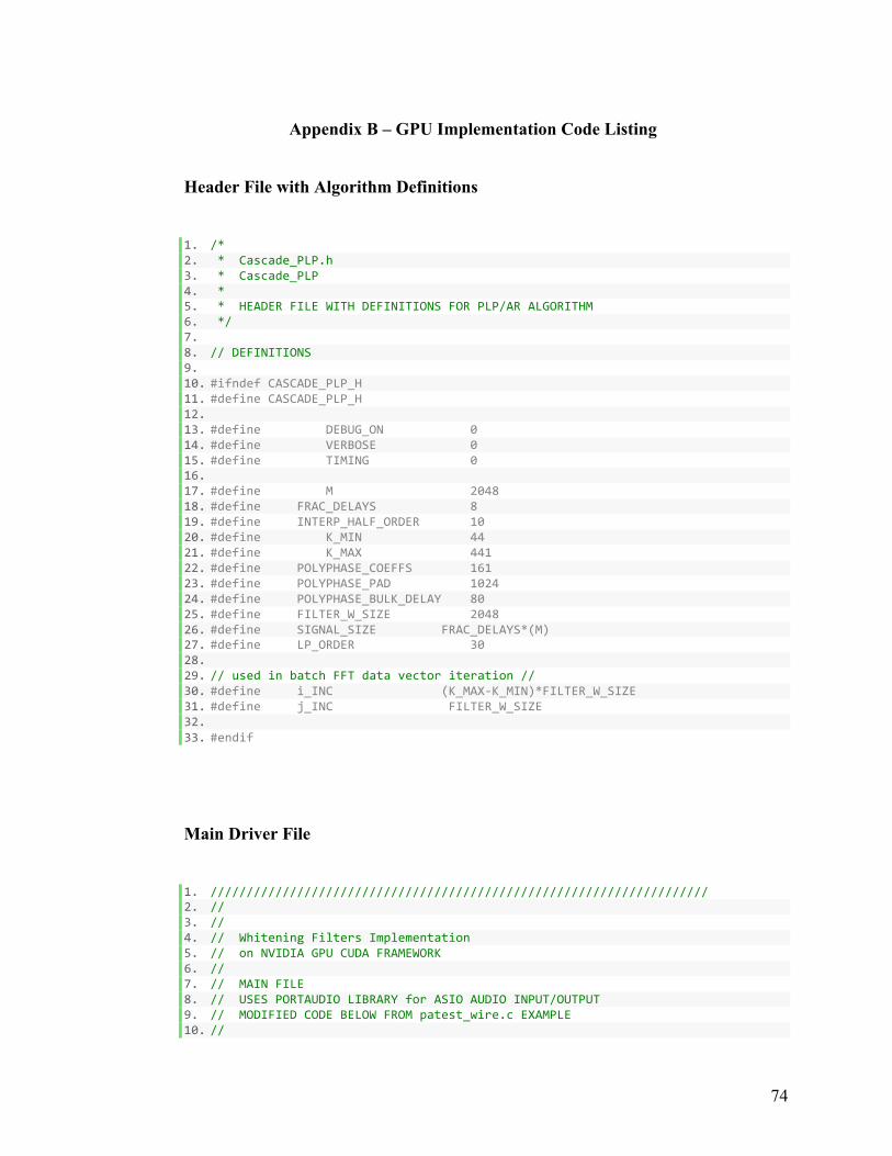
74
Appendix B – GPU Implementation Code Listing
Header File with Algorithm Definitions
1. /* 2. * Cascade_PLP.h 3. * Cascade_PLP 4. * 5. * HEADER FILE WITH DEFINITIONS FOR PLP/AR ALGORITHM 6. */ 7. 8. // DEFINITIONS 9. 10. #ifndef CASCADE_PLP_H 11. #define CASCADE_PLP_H 12. 13. #define DEBUG_ON 0 14. #define VERBOSE 0 15. #define TIMING 0 16. 17. #define M 2048 18. #define FRAC_DELAYS 8 19. #define INTERP_HALF_ORDER 10 20. #define K_MIN 44 21. #define K_MAX 441 22. #define POLYPHASE_COEFFS 161 23. #define POLYPHASE_PAD 1024 24. #define POLYPHASE_BULK_DELAY 80 25. #define FILTER_W_SIZE 2048 26. #define SIGNAL_SIZE FRAC_DELAYS*(M) 27. #define LP_ORDER 30 28. 29. // used in batch FFT data vector iteration // 30. #define i_INC (K_MAX-‐K_MIN)*FILTER_W_SIZE 31. #define j_INC FILTER_W_SIZE 32. 33. #endif
Main Driver File
1. ///////////////////////////////////////////////////////////////////// 2. // 3. // 4. // Whitening Filters Implementation 5. // on NVIDIA GPU CUDA FRAMEWORK 6. // 7. // MAIN FILE 8. // USES PORTAUDIO LIBRARY for ASIO AUDIO INPUT/OUTPUT 9. // MODIFIED CODE BELOW FROM patest_wire.c EXAMPLE 10. //
75
11. // Omer Osman 12. // July 2011 13. // 14. // 15. ///////////////////////////////////////////////////////////////////// 16. 17. /** @file patest_wire.c 18. @ingroup test_src 19. @brief Pass input directly to output. 20. 21. Note that some HW devices, for example many ISA audio cards 22. on PCs, do NOT support full duplex! For a PC, you normally need 23. a PCI based audio card such as the SBLive. 24. 25. @author Phil Burk http://www.softsynth.com 26. 27. While adapting to V19-‐API, I excluded configs with framesPerCallback=0 28. because of an assert in file pa_common/pa_process.c. Pieter, Oct 9, 2003. 29. 30. */ 31. /* 32. * $Id: patest_wire.c 1368 2008-‐03-‐01 00:38:27Z rossb $ 33. * 34. * This program uses the PortAudio Portable Audio Library. 35. * For more information see: http://www.portaudio.com 36. * Copyright (c) 1999-‐2000 Ross Bencina and Phil Burk 37. * 38. * Permission is hereby granted, free of charge, to any person obtaining 39. * a copy of this software and associated documentation files 40. * (the "Software"), to deal in the Software without restriction, 41. * including without limitation the rights to use, copy, modify, merge, 42. * publish, distribute, sublicense, and/or sell copies of the Software, 43. * and to permit persons to whom the Software is furnished to do so, 44. * subject to the following conditions: 45. * 46. * The above copyright notice and this permission notice shall be 47. * included in all copies or substantial portions of the Software. 48. * 49. * THE SOFTWARE IS PROVIDED "AS IS", WITHOUT WARRANTY OF ANY KIND, 50. * EXPRESS OR IMPLIED, INCLUDING BUT NOT LIMITED TO THE WARRANTIES OF 51. * MERCHANTABILITY, FITNESS FOR A PARTICULAR PURPOSE AND NONINFRINGEMENT. 52. * IN NO EVENT SHALL THE AUTHORS OR COPYRIGHT HOLDERS BE LIABLE FOR 53. * ANY CLAIM, DAMAGES OR OTHER LIABILITY, WHETHER IN AN ACTION OF 54. * CONTRACT, TORT OR OTHERWISE, ARISING FROM, OUT OF OR IN CONNECTION 55. * WITH THE SOFTWARE OR THE USE OR OTHER DEALINGS IN THE SOFTWARE. 56. */ 57. 58. /* 59. * The text above constitutes the entire PortAudio license; however, 60. * the PortAudio community also makes the following non-‐binding requests: 61. * 62. * Any person wishing to distribute modifications to the Software is 63. * requested to send the modifications to the original developer so that 64. * they can be incorporated into the canonical version. It is also 65. * requested that these non-‐binding requests be included along with the 66. * license above. 67. */ 68. 69. #include <stdio.h> 70. #include <math.h> 71. #include <iostream>
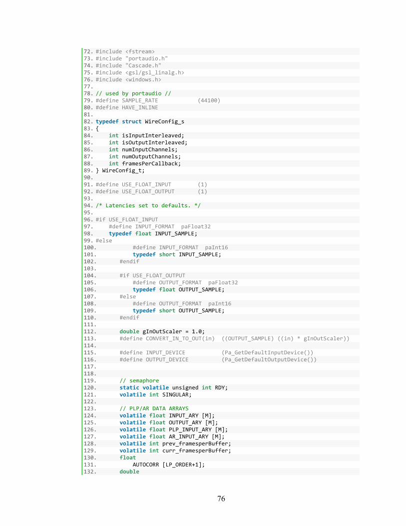
76
72. #include <fstream> 73. #include "portaudio.h" 74. #include "Cascade.h" 75. #include <gsl/gsl_linalg.h> 76. #include <windows.h> 77. 78. // used by portaudio // 79. #define SAMPLE_RATE (44100) 80. #define HAVE_INLINE 81. 82. typedef struct WireConfig_s 83. { 84. int isInputInterleaved; 85. int isOutputInterleaved; 86. int numInputChannels; 87. int numOutputChannels; 88. int framesPerCallback; 89. } WireConfig_t; 90. 91. #define USE_FLOAT_INPUT (1) 92. #define USE_FLOAT_OUTPUT (1) 93. 94. /* Latencies set to defaults. */ 95. 96. #if USE_FLOAT_INPUT 97. #define INPUT_FORMAT paFloat32 98. typedef float INPUT_SAMPLE; 99. #else 100. #define INPUT_FORMAT paInt16 101. typedef short INPUT_SAMPLE; 102. #endif 103. 104. #if USE_FLOAT_OUTPUT 105. #define OUTPUT_FORMAT paFloat32 106. typedef float OUTPUT_SAMPLE; 107. #else 108. #define OUTPUT_FORMAT paInt16 109. typedef short OUTPUT_SAMPLE; 110. #endif 111. 112. double gInOutScaler = 1.0; 113. #define CONVERT_IN_TO_OUT(in) ((OUTPUT_SAMPLE) ((in) * gInOutScaler)) 114. 115. #define INPUT_DEVICE (Pa_GetDefaultInputDevice()) 116. #define OUTPUT_DEVICE (Pa_GetDefaultOutputDevice()) 117. 118. 119. // semaphore 120. static volatile unsigned int RDY; 121. volatile int SINGULAR; 122. 123. // PLP/AR DATA ARRAYS 124. volatile float INPUT_ARY [M]; 125. volatile float OUTPUT_ARY [M]; 126. volatile float PLP_INPUT_ARY [M]; 127. volatile float AR_INPUT_ARY [M]; 128. volatile int prev_framesperBuffer; 129. volatile int curr_framesperBuffer; 130. float 131. AUTOCORR [LP_ORDER+1]; 132. double
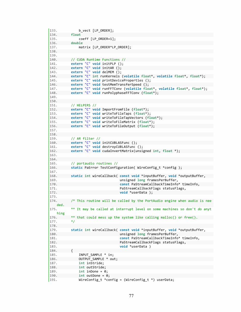
77
133. b_vect [LP_ORDER]; 134. float 135. coeff [LP_ORDER+1]; 136. double 137. matrix [LP_ORDER*LP_ORDER]; 138. 139. 140. // CUDA Runtime Functions // 141. extern "C" void initPLP (); 142. extern "C" void initAR (); 143. extern "C" void delMEM (); 144. extern "C" int runKernels (volatile float*, volatile float*, float*); 145. extern "C" void printDeviceProperties (); 146. extern "C" void testMemTransferSpeed (); 147. extern "C" void runFFTConv (volatile float*, volatile float*, float*); 148. extern "C" void runPolyphaseFFTConv (float*); 149. 150. 151. // HELPERS // 152. extern "C" void ImportFromFile (float*); 153. extern "C" void writeToFileTaps (float*); 154. extern "C" void writeToFileTapVectors (float*); 155. extern "C" void writeToFileMatrix (float*); 156. extern "C" void writeToFileOutput (float*); 157. 158. 159. // AR filter // 160. extern "C" void initCUBLASFunc (); 161. extern "C" void destroyCUBLASFunc (); 162. extern "C" void cudaInvertMatrix(unsigned int, float *); 163. 164. 165. // portaudio routines // 166. static PaError TestConfiguration( WireConfig_t *config ); 167. 168. static int wireCallback( const void *inputBuffer, void *outputBuffer, 169. unsigned long framesPerBuffer, 170. const PaStreamCallbackTimeInfo* timeInfo, 171. PaStreamCallbackFlags statusFlags, 172. void *userData ); 173. 174. /* This routine will be called by the PortAudio engine when audio is nee
ded. 175. ** It may be called at interrupt level on some machines so don't do anyt
hing 176. ** that could mess up the system like calling malloc() or free(). 177. */ 178. 179. static int wireCallback( const void *inputBuffer, void *outputBuffer, 180. unsigned long framesPerBuffer, 181. const PaStreamCallbackTimeInfo* timeInfo, 182. PaStreamCallbackFlags statusFlags, 183. void *userData ) 184. { 185. INPUT_SAMPLE * in; 186. OUTPUT_SAMPLE * out; 187. int inStride; 188. int outStride; 189. int inDone = 0; 190. int outDone = 0; 191. WireConfig_t *config = (WireConfig_t *) userData;
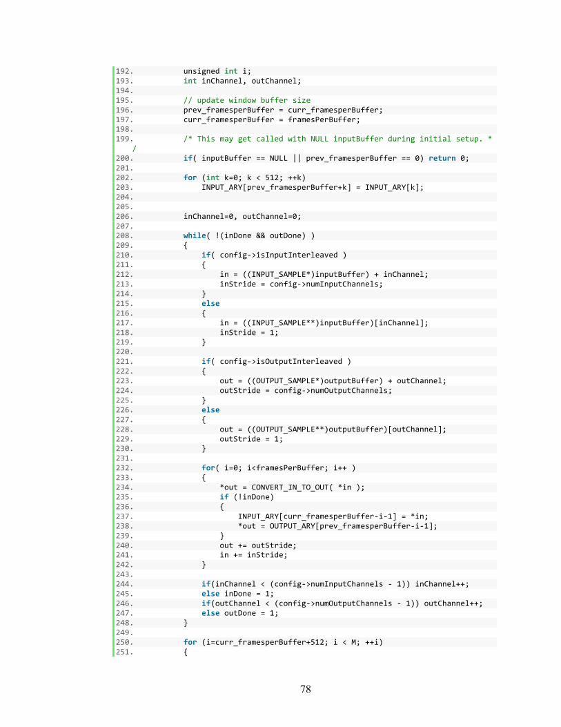
78
192. unsigned int i; 193. int inChannel, outChannel; 194. 195. // update window buffer size 196. prev_framesperBuffer = curr_framesperBuffer; 197. curr_framesperBuffer = framesPerBuffer; 198. 199. /* This may get called with NULL inputBuffer during initial setup. *
/ 200. if( inputBuffer == NULL || prev_framesperBuffer == 0) return 0; 201. 202. for (int k=0; k < 512; ++k) 203. INPUT_ARY[prev_framesperBuffer+k] = INPUT_ARY[k]; 204. 205. 206. inChannel=0, outChannel=0; 207. 208. while( !(inDone && outDone) ) 209. { 210. if( config-‐>isInputInterleaved ) 211. { 212. in = ((INPUT_SAMPLE*)inputBuffer) + inChannel; 213. inStride = config-‐>numInputChannels; 214. } 215. else 216. { 217. in = ((INPUT_SAMPLE**)inputBuffer)[inChannel]; 218. inStride = 1; 219. } 220. 221. if( config-‐>isOutputInterleaved ) 222. { 223. out = ((OUTPUT_SAMPLE*)outputBuffer) + outChannel; 224. outStride = config-‐>numOutputChannels; 225. } 226. else 227. { 228. out = ((OUTPUT_SAMPLE**)outputBuffer)[outChannel]; 229. outStride = 1; 230. } 231. 232. for( i=0; i<framesPerBuffer; i++ ) 233. { 234. *out = CONVERT_IN_TO_OUT( *in ); 235. if (!inDone) 236. { 237. INPUT_ARY[curr_framesperBuffer-‐i-‐1] = *in; 238. *out = OUTPUT_ARY[prev_framesperBuffer-‐i-‐1]; 239. } 240. out += outStride; 241. in += inStride; 242. } 243. 244. if(inChannel < (config-‐>numInputChannels -‐ 1)) inChannel++; 245. else inDone = 1; 246. if(outChannel < (config-‐>numOutputChannels -‐ 1)) outChannel++; 247. else outDone = 1; 248. } 249. 250. for (i=curr_framesperBuffer+512; i < M; ++i) 251. {
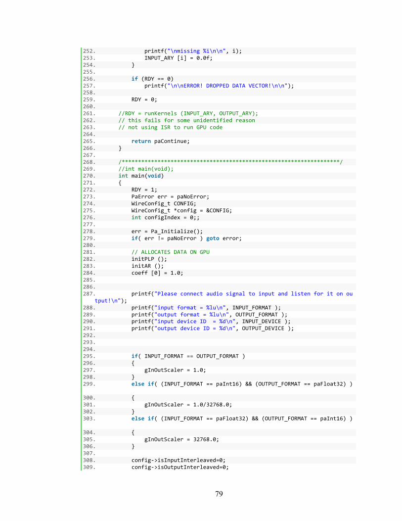
79
252. printf("\nmissing %i\n\n", i); 253. INPUT_ARY [i] = 0.0f; 254. } 255. 256. if (RDY == 0) 257. printf("\n\nERROR! DROPPED DATA VECTOR!\n\n"); 258. 259. RDY = 0; 260. 261. //RDY = runKernels (INPUT_ARY, OUTPUT_ARY); 262. // this fails for some unidentified reason 263. // not using ISR to run GPU code 264. 265. return paContinue; 266. } 267. 268. /*******************************************************************/ 269. //int main(void); 270. int main(void) 271. { 272. RDY = 1; 273. PaError err = paNoError; 274. WireConfig_t CONFIG; 275. WireConfig_t *config = &CONFIG; 276. int configIndex = 0;; 277. 278. err = Pa_Initialize(); 279. if( err != paNoError ) goto error; 280. 281. // ALLOCATES DATA ON GPU 282. initPLP (); 283. initAR (); 284. coeff [0] = 1.0; 285. 286. 287. printf("Please connect audio signal to input and listen for it on ou
tput!\n"); 288. printf("input format = %lu\n", INPUT_FORMAT ); 289. printf("output format = %lu\n", OUTPUT_FORMAT ); 290. printf("input device ID = %d\n", INPUT_DEVICE ); 291. printf("output device ID = %d\n", OUTPUT_DEVICE ); 292. 293. 294. 295. if( INPUT_FORMAT == OUTPUT_FORMAT ) 296. { 297. gInOutScaler = 1.0; 298. } 299. else if( (INPUT_FORMAT == paInt16) && (OUTPUT_FORMAT == paFloat32) )
300. { 301. gInOutScaler = 1.0/32768.0; 302. } 303. else if( (INPUT_FORMAT == paFloat32) && (OUTPUT_FORMAT == paInt16) )
304. { 305. gInOutScaler = 32768.0; 306. } 307. 308. config-‐>isInputInterleaved=0; 309. config-‐>isOutputInterleaved=0;
80
310. config-‐>numInputChannels=1; 311. config-‐>numOutputChannels=2; 312. config-‐>framesPerCallback=1536; 313. 314. 315. 316. printf("-‐-‐-‐-‐-‐-‐-‐-‐-‐-‐-‐-‐-‐-‐-‐-‐-‐-‐-‐-‐-‐-‐-‐-‐-‐-‐-‐-‐-‐-‐-‐-‐-‐-‐-‐-‐-‐-‐-‐-‐-‐-‐-‐-‐-‐-‐-‐\n" ); 317. printf("Configuration #%d\n", configIndex++ ); 318. err = TestConfiguration( config ); 319. /* Give user a chance to bail out. */ 320. 321. if( err == 1 ) 322. { 323. err = paNoError; 324. goto done; 325. } 326. else if( err != paNoError ) goto error; 327. 328. done: 329. Pa_Terminate(); 330. delMEM (); 331. // destroyCUBLASFunc (); 332. // free(matrix); 333. printf("\naudio streaming complete.\n"); fflush(stdout); 334. return 0; 335. 336. error: 337. Pa_Terminate(); 338. fprintf( stderr, "An error occured while using the portaudio stream\
n" ); 339. fprintf( stderr, "Error number: %d\n", err ); 340. fprintf( stderr, "Error message: %s\n", Pa_GetErrorText( err ) ); 341. printf("Hit ENTER to quit.\n"); fflush(stdout); 342. getchar(); 343. return -‐1; 344. } 345. 346. static PaError TestConfiguration( WireConfig_t *config ) 347. { 348. int c; 349. PaError err = paNoError; 350. PaStream *stream; 351. PaStreamParameters inputParameters, outputParameters; 352. 353. printf("input %sinterleaved!\n", (config-‐
>isInputInterleaved ? " " : "NOT ") ); 354. printf("output %sinterleaved!\n", (config-‐
>isOutputInterleaved ? " " : "NOT ") ); 355. printf("input channels = %d\n", config-‐>numInputChannels ); 356. printf("output channels = %d\n", config-‐>numOutputChannels ); 357. printf("framesPerCallback = %d\n", config-‐>framesPerCallback ); 358. 359. inputParameters.device = INPUT_DEVICE; /* default input
device */ 360. if (inputParameters.device == paNoDevice) { 361. fprintf(stderr,"Error: No default input device.\n"); 362. goto error; 363. } 364. inputParameters.channelCount = config-‐>numInputChannels; 365. inputParameters.sampleFormat = INPUT_FORMAT | (config-‐
>isInputInterleaved ? 0 : paNonInterleaved);
81
366. inputParameters.suggestedLatency = Pa_GetDeviceInfo( inputParameters.device )-‐>defaultLowInputLatency;
367. printf ("Input Latency %f\n", inputParameters.suggestedLatency); 368. inputParameters.hostApiSpecificStreamInfo = NULL; 369. 370. outputParameters.device = OUTPUT_DEVICE; /* default outpu
t device */ 371. if (outputParameters.device == paNoDevice) { 372. fprintf(stderr,"Error: No default output device.\n"); 373. goto error; 374. } 375. outputParameters.channelCount = config-‐>numOutputChannels; 376. outputParameters.sampleFormat = OUTPUT_FORMAT | (config-‐
>isOutputInterleaved ? 0 : paNonInterleaved); 377. outputParameters.suggestedLatency = Pa_GetDeviceInfo( outputParamete
rs.device )-‐>defaultLowOutputLatency; 378. printf ("Output Latency %f\n", outputParameters.suggestedLatency); 379. outputParameters.hostApiSpecificStreamInfo = NULL; 380. 381. err = Pa_OpenStream( 382. &stream, 383. &inputParameters, 384. &outputParameters, 385. SAMPLE_RATE, 386. config-‐>framesPerCallback, /* frames per buffer */ 387. paClipOff, /* we won't output out of range samples so don'
t bother clipping them */ 388. wireCallback, 389. config ); 390. if( err != paNoError ) goto error; 391. 392. printf("\nStarting audio stream...\n"); 393. 394. printf("Hit ENTER to start processing\n\n"); fflush(stdout); 395. c = getchar(); 396. 397. err = Pa_StartStream( stream ); 398. if( err != paNoError ) goto error; 399. 400. 401. gsl_vector * 402. x = gsl_vector_alloc (LP_ORDER); 403. gsl_permutation * 404. p = gsl_permutation_alloc (LP_ORDER); 405. 406. gsl_matrix_view 407. m; 408. gsl_vector_view 409. b; 410. int s; 411. LONGLONG Freq; 412. LONGLONG Now; 413. LONGLONG Last; 414. 415. 416. while (1) 417. { 418. if (RDY == 0) 419. { 420. // PreWhitening 421. runFFTConv (INPUT_ARY, PLP_INPUT_ARY, coeff);
82
422. 423. // PLP Filter 424. RDY = runKernels (PLP_INPUT_ARY, AR_INPUT_ARY, AUTOCORR); 425. 426. if (SINGULAR != 1) 427. { 428. // set AR_INPUT_ARY to OUTPUT_ARY 429. if (TIMING) 430. { 431. QueryPerformanceFrequency ( reinterpret_cast<LARGE_I
NTEGER*>(&Freq) ); 432. QueryPerformanceCounter( reinterpret_cast<LARGE_INTE
GER*>(&Last) ); 433. } 434. 435. // AR FILTER IMPLEMENTATION USING GNU SCIENTIFIC LIBRARY
-‐-‐GSL 436. // AUTOCORR vector computed in GPU in frequency domain 437. for (int i=0; i < (LP_ORDER); ++i) 438. for (int j=i; j < (LP_ORDER); ++j) 439. { 440. matrix[i+(LP_ORDER)*j] = AUTOCORR[j-‐i]; 441. matrix[j+i*(LP_ORDER)] = AUTOCORR[j-‐i]; 442. } 443. 444. for (int i=0; i < LP_ORDER; ++i) 445. { 446. b_vect[i] = -‐AUTOCORR[i+1]; 447. } 448. 449. m = gsl_matrix_view_array(matrix, LP_ORDER, LP_ORDER); 450. b = gsl_vector_view_array(b_vect, LP_ORDER); 451. 452. // matrix inversion using LU decomp 453. gsl_linalg_LU_decomp (&m.matrix, p, &s); 454. gsl_linalg_LU_solve (&m.matrix, p, &b.vector, x); 455. 456. coeff[0] = 1.0; 457. for (int i=0; i < LP_ORDER; ++i) 458. coeff[i+1] = gsl_vector_get(x, i); 459. 460. 461. if (TIMING) 462. { 463. QueryPerformanceCounter( reinterpret_cast<LARGE_INTE
GER*>(&Now) ); 464. LONGLONG EclapsedCount = Now -‐ Last; 465. LONGLONG TimerResolution = 1000; //Milliseconds 466. double Milliseconds = EclapsedCount * TimerResolutio
n / (double)Freq; 467. printf("Matrix Inversion Run speed: %3.3f ms\n", Mil
liseconds); 468. } 469. 470. runFFTConv (AR_INPUT_ARY, OUTPUT_ARY, coeff); 471. writeToFileOutput ((float*)OUTPUT_ARY); 472. getchar(); 473. } 474. else 475. { 476. for (int i=0; i < FILTER_W_SIZE; ++i)
83
477. OUTPUT_ARY [i] = INPUT_ARY[i]; 478. SINGULAR = 0; 479. } 480. 481. } 482. } 483. 484. gsl_permutation_free (p); 485. gsl_vector_free(x); 486. 487. 488. done: 489. printf("Closing stream.\n"); 490. err = Pa_CloseStream( stream ); 491. if( err != paNoError ) goto error; 492. return 1; 493. 494. error: 495. return err; 496. 497. } 498. 499. 500. 501. // helpers 502. void ImportFromFile (float* MyNumbers) 503. { 504. std::fstream 505. myfile; 506. 507. myfile.open("res_filters.dat"); 508. 509. for (int i=0; i < K_MAX-‐K_MIN; ++i) { 510. for (int j=0; j < 8; ++j) { 511. for (int k=0; k < 512; ++k) { 512. myfile >> (MyNumbers)[(i*8)+(j*512)+k]; 513. } 514. } 515. } 516. 517. myfile.close(); 518. 519. return; 520. } 521. 522. void writeToFileTaps (float* H_ResidualFilterTaps) 523. { 524. std :: ofstream 525. myfile; 526. 527. myfile.open ("taps.dat"); 528. 529. for (int i=0; i < (K_MAX-‐K_MIN); ++i) 530. { 531. for (int j=0; j < 8; ++j) { 532. myfile << (H_ResidualFilterTaps)[(i*8)+j]; 533. myfile << " "; 534. } 535. myfile << std :: endl; 536. } 537. myfile.close();
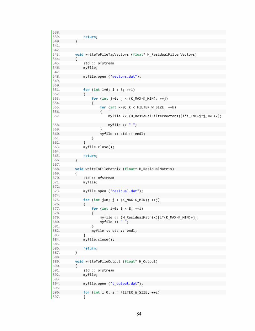
84
538. 539. return; 540. } 541. 542. 543. void writeToFileTapVectors (float* H_ResidualFilterVectors) 544. { 545. std :: ofstream 546. myfile; 547. 548. myfile.open ("vectors.dat"); 549. 550. 551. for (int i=0; i < 8; ++i) 552. { 553. for (int j=0; j < (K_MAX-‐K_MIN); ++j) 554. { 555. for (int k=0; k < FILTER_W_SIZE; ++k) 556. { 557. myfile << (H_ResidualFilterVectors)[i*i_INC+j*j_INC+k];
558. myfile << " "; 559. } 560. myfile << std :: endl; 561. } 562. } 563. myfile.close(); 564. 565. return; 566. } 567. 568. void writeToFileMatrix (float* H_ResidualMatrix) 569. { 570. std :: ofstream 571. myfile; 572. 573. myfile.open ("residual.dat"); 574. 575. for (int j=0; j < (K_MAX-‐K_MIN); ++j) 576. { 577. for (int i=0; i < 8; ++i) 578. { 579. myfile << (H_ResidualMatrix)[i*(K_MAX-‐K_MIN)+j]; 580. myfile << " "; 581. } 582. myfile << std :: endl; 583. } 584. myfile.close(); 585. 586. return; 587. } 588. 589. void writeToFileOutput (float* H_Output) 590. { 591. std :: ofstream 592. myfile; 593. 594. myfile.open ("t_output.dat"); 595. 596. for (int i=0; i < FILTER_W_SIZE; ++i) 597. {
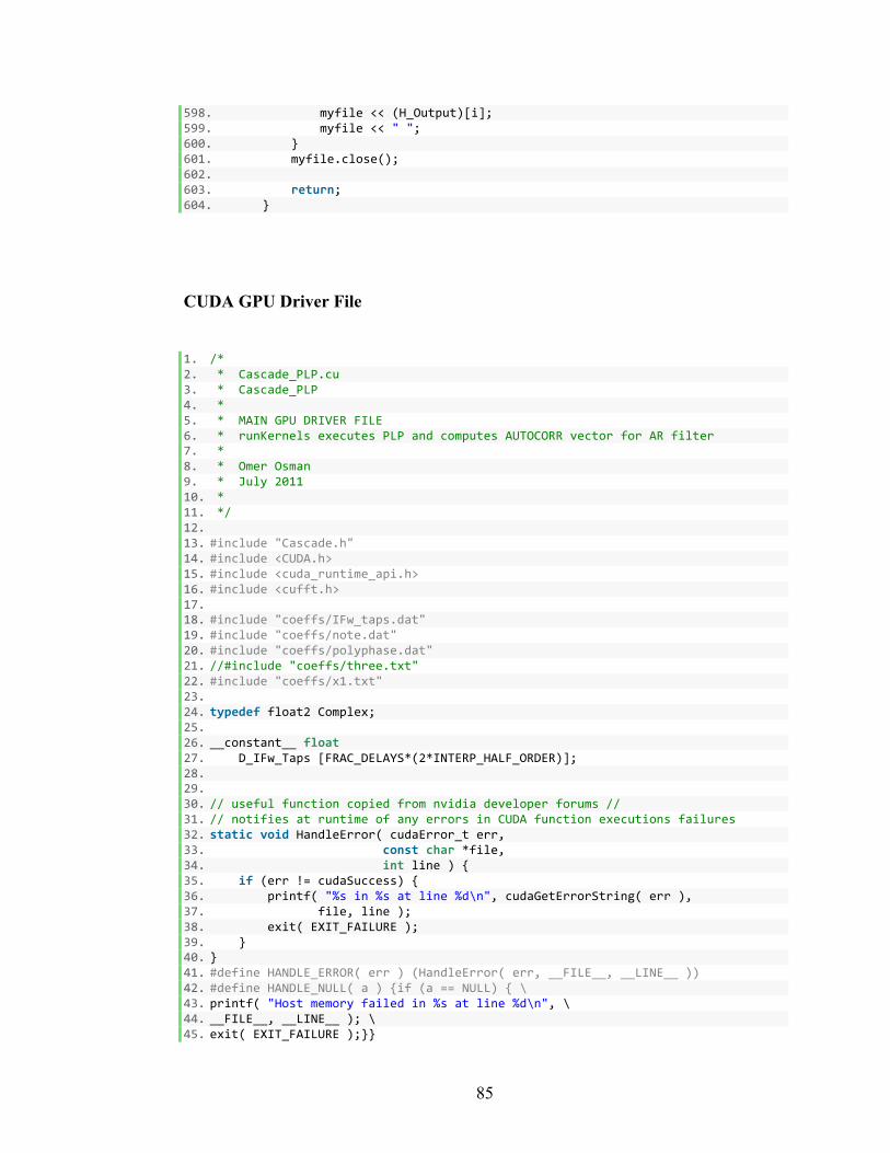
85
598. myfile << (H_Output)[i]; 599. myfile << " "; 600. } 601. myfile.close(); 602. 603. return; 604. }
CUDA GPU Driver File
1. /* 2. * Cascade_PLP.cu 3. * Cascade_PLP 4. * 5. * MAIN GPU DRIVER FILE 6. * runKernels executes PLP and computes AUTOCORR vector for AR filter 7. * 8. * Omer Osman 9. * July 2011 10. * 11. */ 12. 13. #include "Cascade.h" 14. #include <CUDA.h> 15. #include <cuda_runtime_api.h> 16. #include <cufft.h> 17. 18. #include "coeffs/IFw_taps.dat" 19. #include "coeffs/note.dat" 20. #include "coeffs/polyphase.dat" 21. //#include "coeffs/three.txt" 22. #include "coeffs/x1.txt" 23. 24. typedef float2 Complex; 25. 26. __constant__ float 27. D_IFw_Taps [FRAC_DELAYS*(2*INTERP_HALF_ORDER)]; 28. 29. 30. // useful function copied from nvidia developer forums // 31. // notifies at runtime of any errors in CUDA function executions failures 32. static void HandleError( cudaError_t err, 33. const char *file, 34. int line ) { 35. if (err != cudaSuccess) { 36. printf( "%s in %s at line %d\n", cudaGetErrorString( err ), 37. file, line ); 38. exit( EXIT_FAILURE ); 39. } 40. } 41. #define HANDLE_ERROR( err ) (HandleError( err, __FILE__, __LINE__ )) 42. #define HANDLE_NULL( a ) {if (a == NULL) { \ 43. printf( "Host memory failed in %s at line %d\n", \ 44. __FILE__, __LINE__ ); \ 45. exit( EXIT_FAILURE );}}
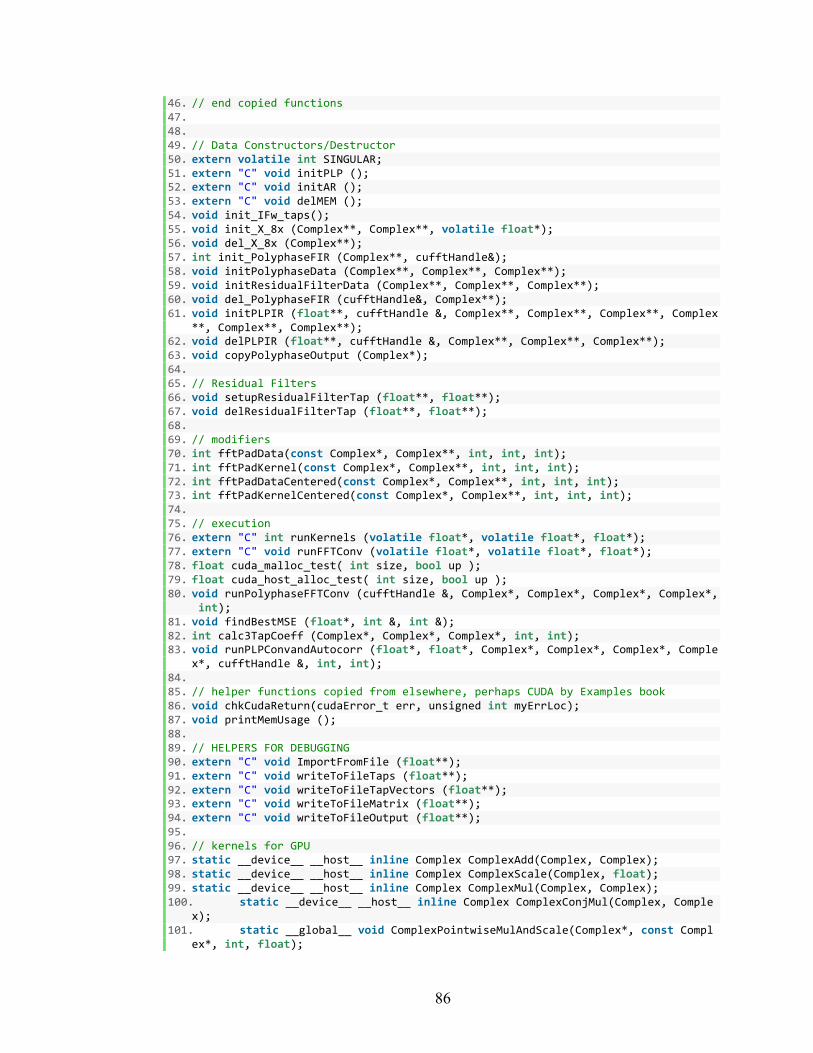
86
46. // end copied functions 47. 48. 49. // Data Constructors/Destructor 50. extern volatile int SINGULAR; 51. extern "C" void initPLP (); 52. extern "C" void initAR (); 53. extern "C" void delMEM (); 54. void init_IFw_taps(); 55. void init_X_8x (Complex**, Complex**, volatile float*); 56. void del_X_8x (Complex**); 57. int init_PolyphaseFIR (Complex**, cufftHandle&); 58. void initPolyphaseData (Complex**, Complex**, Complex**); 59. void initResidualFilterData (Complex**, Complex**, Complex**); 60. void del_PolyphaseFIR (cufftHandle&, Complex**); 61. void initPLPIR (float**, cufftHandle &, Complex**, Complex**, Complex**, Complex
**, Complex**, Complex**); 62. void delPLPIR (float**, cufftHandle &, Complex**, Complex**, Complex**); 63. void copyPolyphaseOutput (Complex*); 64. 65. // Residual Filters 66. void setupResidualFilterTap (float**, float**); 67. void delResidualFilterTap (float**, float**); 68. 69. // modifiers 70. int fftPadData(const Complex*, Complex**, int, int, int); 71. int fftPadKernel(const Complex*, Complex**, int, int, int); 72. int fftPadDataCentered(const Complex*, Complex**, int, int, int); 73. int fftPadKernelCentered(const Complex*, Complex**, int, int, int); 74. 75. // execution 76. extern "C" int runKernels (volatile float*, volatile float*, float*); 77. extern "C" void runFFTConv (volatile float*, volatile float*, float*); 78. float cuda_malloc_test( int size, bool up ); 79. float cuda_host_alloc_test( int size, bool up ); 80. void runPolyphaseFFTConv (cufftHandle &, Complex*, Complex*, Complex*, Complex*,
int); 81. void findBestMSE (float*, int &, int &); 82. int calc3TapCoeff (Complex*, Complex*, Complex*, int, int); 83. void runPLPConvandAutocorr (float*, float*, Complex*, Complex*, Complex*, Comple
x*, cufftHandle &, int, int); 84. 85. // helper functions copied from elsewhere, perhaps CUDA by Examples book 86. void chkCudaReturn(cudaError_t err, unsigned int myErrLoc); 87. void printMemUsage (); 88. 89. // HELPERS FOR DEBUGGING 90. extern "C" void ImportFromFile (float**); 91. extern "C" void writeToFileTaps (float**); 92. extern "C" void writeToFileTapVectors (float**); 93. extern "C" void writeToFileMatrix (float**); 94. extern "C" void writeToFileOutput (float**); 95. 96. // kernels for GPU 97. static __device__ __host__ inline Complex ComplexAdd(Complex, Complex); 98. static __device__ __host__ inline Complex ComplexScale(Complex, float); 99. static __device__ __host__ inline Complex ComplexMul(Complex, Complex); 100. static __device__ __host__ inline Complex ComplexConjMul(Complex, Comple
x); 101. static __global__ void ComplexPointwiseMulAndScale(Complex*, const Compl
ex*, int, float);
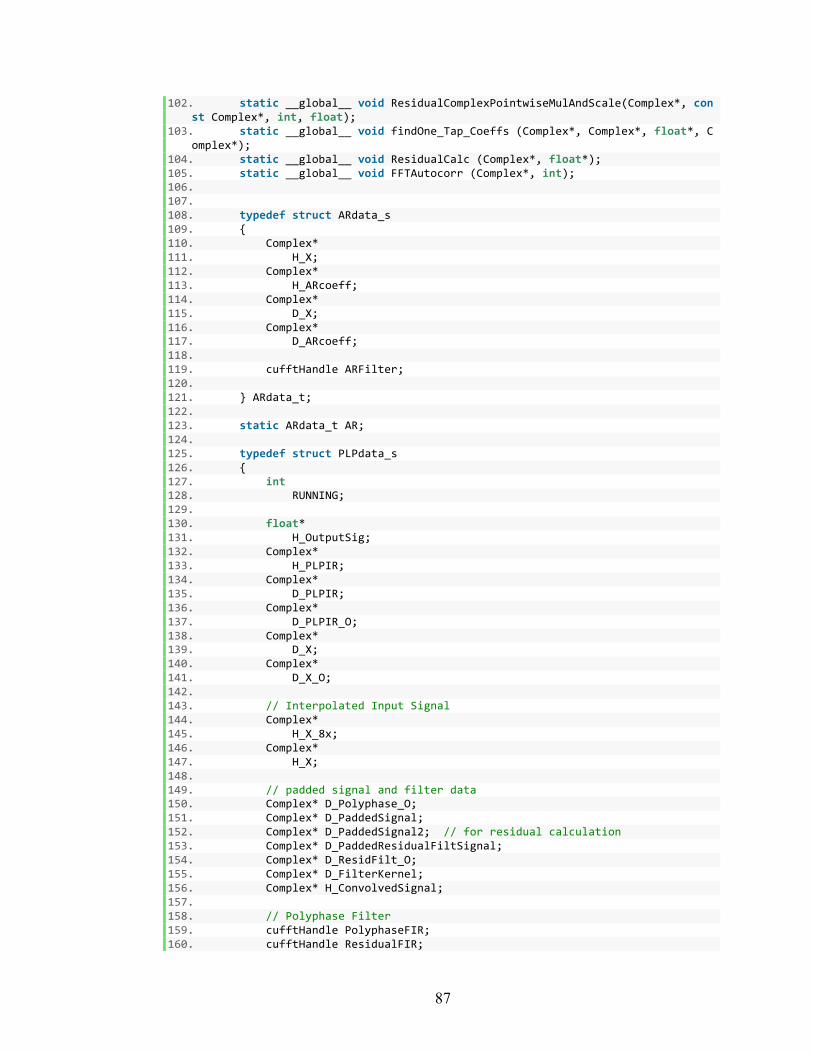
87
102. static __global__ void ResidualComplexPointwiseMulAndScale(Complex*, const Complex*, int, float);
103. static __global__ void findOne_Tap_Coeffs (Complex*, Complex*, float*, Complex*);
104. static __global__ void ResidualCalc (Complex*, float*); 105. static __global__ void FFTAutocorr (Complex*, int); 106. 107. 108. typedef struct ARdata_s 109. { 110. Complex* 111. H_X; 112. Complex* 113. H_ARcoeff; 114. Complex* 115. D_X; 116. Complex* 117. D_ARcoeff; 118. 119. cufftHandle ARFilter; 120. 121. } ARdata_t; 122. 123. static ARdata_t AR; 124. 125. typedef struct PLPdata_s 126. { 127. int 128. RUNNING; 129. 130. float* 131. H_OutputSig; 132. Complex* 133. H_PLPIR; 134. Complex* 135. D_PLPIR; 136. Complex* 137. D_PLPIR_O; 138. Complex* 139. D_X; 140. Complex* 141. D_X_O; 142. 143. // Interpolated Input Signal 144. Complex* 145. H_X_8x; 146. Complex* 147. H_X; 148. 149. // padded signal and filter data 150. Complex* D_Polyphase_O; 151. Complex* D_PaddedSignal; 152. Complex* D_PaddedSignal2; // for residual calculation 153. Complex* D_PaddedResidualFiltSignal; 154. Complex* D_ResidFilt_O; 155. Complex* D_FilterKernel; 156. Complex* H_ConvolvedSignal; 157. 158. // Polyphase Filter 159. cufftHandle PolyphaseFIR; 160. cufftHandle ResidualFIR;
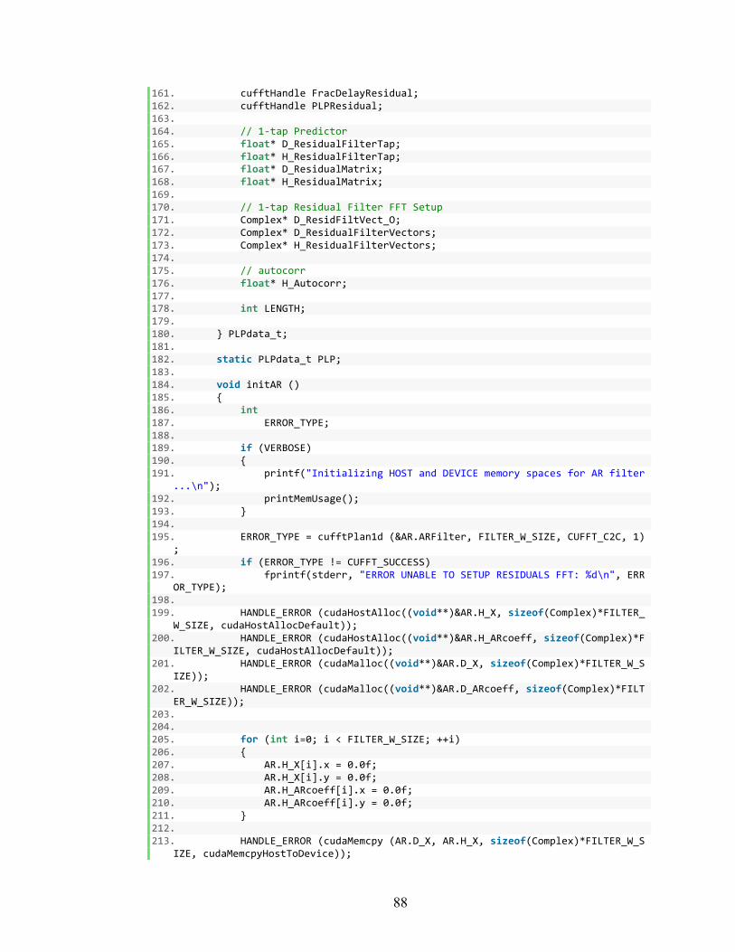
88
161. cufftHandle FracDelayResidual; 162. cufftHandle PLPResidual; 163. 164. // 1-‐tap Predictor 165. float* D_ResidualFilterTap; 166. float* H_ResidualFilterTap; 167. float* D_ResidualMatrix; 168. float* H_ResidualMatrix; 169. 170. // 1-‐tap Residual Filter FFT Setup 171. Complex* D_ResidFiltVect_O; 172. Complex* D_ResidualFilterVectors; 173. Complex* H_ResidualFilterVectors; 174. 175. // autocorr 176. float* H_Autocorr; 177. 178. int LENGTH; 179. 180. } PLPdata_t; 181. 182. static PLPdata_t PLP; 183. 184. void initAR () 185. { 186. int 187. ERROR_TYPE; 188. 189. if (VERBOSE) 190. { 191. printf("Initializing HOST and DEVICE memory spaces for AR filter
...\n"); 192. printMemUsage(); 193. } 194. 195. ERROR_TYPE = cufftPlan1d (&AR.ARFilter, FILTER_W_SIZE, CUFFT_C2C, 1)
; 196. if (ERROR_TYPE != CUFFT_SUCCESS) 197. fprintf(stderr, "ERROR UNABLE TO SETUP RESIDUALS FFT: %d\n", ERR
OR_TYPE); 198. 199. HANDLE_ERROR (cudaHostAlloc((void**)&AR.H_X, sizeof(Complex)*FILTER_
W_SIZE, cudaHostAllocDefault)); 200. HANDLE_ERROR (cudaHostAlloc((void**)&AR.H_ARcoeff, sizeof(Complex)*F
ILTER_W_SIZE, cudaHostAllocDefault)); 201. HANDLE_ERROR (cudaMalloc((void**)&AR.D_X, sizeof(Complex)*FILTER_W_S
IZE)); 202. HANDLE_ERROR (cudaMalloc((void**)&AR.D_ARcoeff, sizeof(Complex)*FILT
ER_W_SIZE)); 203. 204. 205. for (int i=0; i < FILTER_W_SIZE; ++i) 206. { 207. AR.H_X[i].x = 0.0f; 208. AR.H_X[i].y = 0.0f; 209. AR.H_ARcoeff[i].x = 0.0f; 210. AR.H_ARcoeff[i].y = 0.0f; 211. } 212. 213. HANDLE_ERROR (cudaMemcpy (AR.D_X, AR.H_X, sizeof(Complex)*FILTER_W_S
IZE, cudaMemcpyHostToDevice));
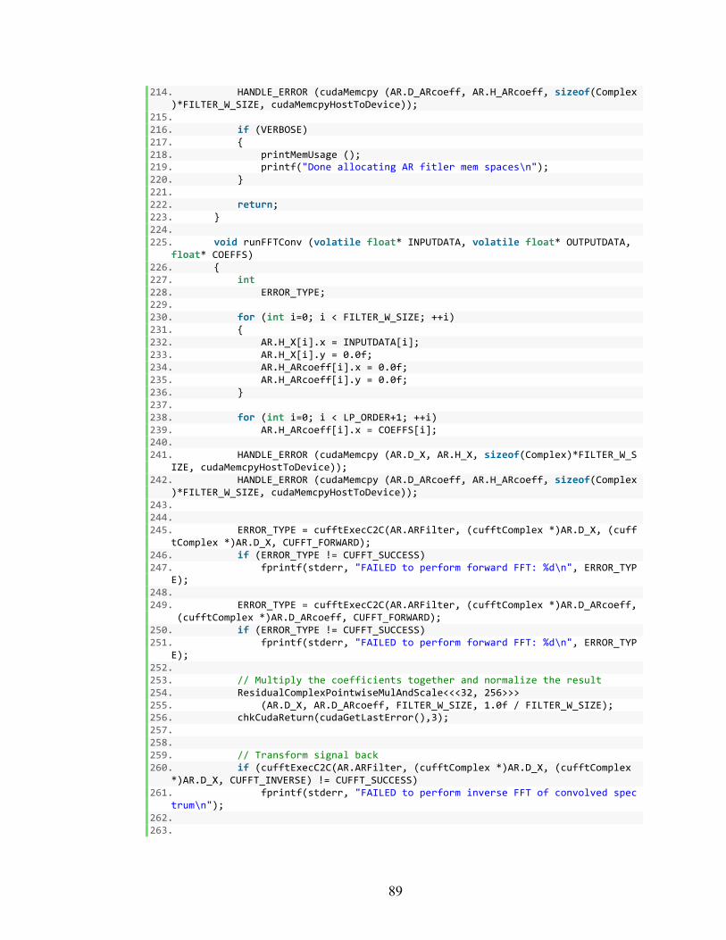
89
214. HANDLE_ERROR (cudaMemcpy (AR.D_ARcoeff, AR.H_ARcoeff, sizeof(Complex)*FILTER_W_SIZE, cudaMemcpyHostToDevice));
215. 216. if (VERBOSE) 217. { 218. printMemUsage (); 219. printf("Done allocating AR fitler mem spaces\n"); 220. } 221. 222. return; 223. } 224. 225. void runFFTConv (volatile float* INPUTDATA, volatile float* OUTPUTDATA,
float* COEFFS) 226. { 227. int 228. ERROR_TYPE; 229. 230. for (int i=0; i < FILTER_W_SIZE; ++i) 231. { 232. AR.H_X[i].x = INPUTDATA[i]; 233. AR.H_X[i].y = 0.0f; 234. AR.H_ARcoeff[i].x = 0.0f; 235. AR.H_ARcoeff[i].y = 0.0f; 236. } 237. 238. for (int i=0; i < LP_ORDER+1; ++i) 239. AR.H_ARcoeff[i].x = COEFFS[i]; 240. 241. HANDLE_ERROR (cudaMemcpy (AR.D_X, AR.H_X, sizeof(Complex)*FILTER_W_S
IZE, cudaMemcpyHostToDevice)); 242. HANDLE_ERROR (cudaMemcpy (AR.D_ARcoeff, AR.H_ARcoeff, sizeof(Complex
)*FILTER_W_SIZE, cudaMemcpyHostToDevice)); 243. 244. 245. ERROR_TYPE = cufftExecC2C(AR.ARFilter, (cufftComplex *)AR.D_X, (cuff
tComplex *)AR.D_X, CUFFT_FORWARD); 246. if (ERROR_TYPE != CUFFT_SUCCESS) 247. fprintf(stderr, "FAILED to perform forward FFT: %d\n", ERROR_TYP
E); 248. 249. ERROR_TYPE = cufftExecC2C(AR.ARFilter, (cufftComplex *)AR.D_ARcoeff,
(cufftComplex *)AR.D_ARcoeff, CUFFT_FORWARD); 250. if (ERROR_TYPE != CUFFT_SUCCESS) 251. fprintf(stderr, "FAILED to perform forward FFT: %d\n", ERROR_TYP
E); 252. 253. // Multiply the coefficients together and normalize the result 254. ResidualComplexPointwiseMulAndScale<<<32, 256>>> 255. (AR.D_X, AR.D_ARcoeff, FILTER_W_SIZE, 1.0f / FILTER_W_SIZE); 256. chkCudaReturn(cudaGetLastError(),3); 257. 258. 259. // Transform signal back 260. if (cufftExecC2C(AR.ARFilter, (cufftComplex *)AR.D_X, (cufftComplex
*)AR.D_X, CUFFT_INVERSE) != CUFFT_SUCCESS) 261. fprintf(stderr, "FAILED to perform inverse FFT of convolved spec
trum\n"); 262. 263.
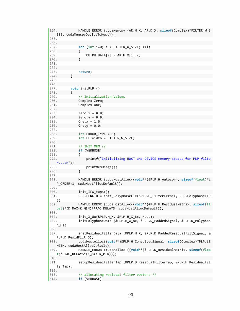
90
264. HANDLE_ERROR (cudaMemcpy (AR.H_X, AR.D_X, sizeof(Complex)*FILTER_W_SIZE, cudaMemcpyDeviceToHost));
265. 266. 267. for (int i=0; i < FILTER_W_SIZE; ++i) 268. { 269. OUTPUTDATA[i] = AR.H_X[i].x; 270. } 271. 272. 273. return; 274. } 275. 276. 277. void initPLP () 278. { 279. // Initialization Values 280. Complex Zero; 281. Complex One; 282. 283. Zero.x = 0.0; 284. Zero.y = 0.0; 285. One.x = 1.0; 286. One.y = 0.0; 287. 288. int ERROR_TYPE = 0; 289. int FFTwidth = FILTER_W_SIZE; 290. 291. // INIT MEM // 292. if (VERBOSE) 293. { 294. printf("Initializing HOST and DEVICE memory spaces for PLP filte
r...\n"); 295. printMemUsage(); 296. } 297. 298. HANDLE_ERROR (cudaHostAlloc((void**)&PLP.H_Autocorr, sizeof(float)*L
P_ORDER+1, cudaHostAllocDefault)); 299. 300. init_IFw_taps(); 301. PLP.LENGTH = init_PolyphaseFIR(&PLP.D_FilterKernel, PLP.PolyphaseFIR
); 302. HANDLE_ERROR (cudaHostAlloc((void**)&PLP.H_ResidualMatrix, sizeof(fl
oat)*(K_MAX-‐K_MIN)*FRAC_DELAYS, cudaHostAllocDefault)); 303. 304. init_X_8x(&PLP.H_X, &PLP.H_X_8x, NULL); 305. initPolyphaseData (&PLP.H_X_8x, &PLP.D_PaddedSignal, &PLP.D_Polyphas
e_O); 306. 307. initResidualFilterData (&PLP.H_X, &PLP.D_PaddedResidualFiltSignal, &
PLP.D_ResidFilt_O); 308. cudaHostAlloc((void**)&PLP.H_ConvolvedSignal, sizeof(Complex)*PLP.LE
NGTH, cudaHostAllocDefault); 309. HANDLE_ERROR (cudaMalloc ((void**)&PLP.D_ResidualMatrix, sizeof(floa
t)*FRAC_DELAYS*(K_MAX-‐K_MIN))); 310. 311. setupResidualFilterTap (&PLP.D_ResidualFilterTap, &PLP.H_ResidualFil
terTap); 312. 313. // allocating residual filter vectors // 314. if (VERBOSE)
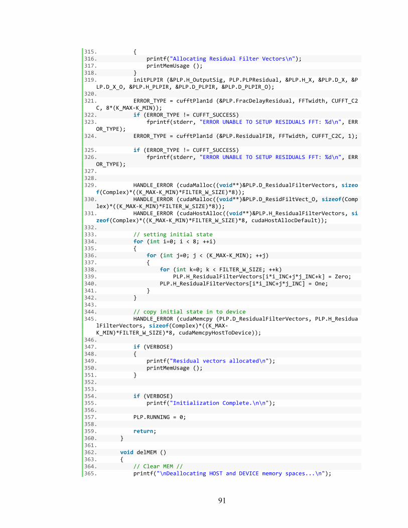
91
315. { 316. printf("Allocating Residual Filter Vectors\n"); 317. printMemUsage (); 318. } 319. initPLPIR (&PLP.H_OutputSig, PLP.PLPResidual, &PLP.H_X, &PLP.D_X, &P
LP.D_X_O, &PLP.H_PLPIR, &PLP.D_PLPIR, &PLP.D_PLPIR_O); 320. 321. ERROR_TYPE = cufftPlan1d (&PLP.FracDelayResidual, FFTwidth, CUFFT_C2
C, 8*(K_MAX-‐K_MIN)); 322. if (ERROR_TYPE != CUFFT_SUCCESS) 323. fprintf(stderr, "ERROR UNABLE TO SETUP RESIDUALS FFT: %d\n", ERR
OR_TYPE); 324. ERROR_TYPE = cufftPlan1d (&PLP.ResidualFIR, FFTwidth, CUFFT_C2C, 1);
325. if (ERROR_TYPE != CUFFT_SUCCESS) 326. fprintf(stderr, "ERROR UNABLE TO SETUP RESIDUALS FFT: %d\n", ERR
OR_TYPE); 327. 328. 329. HANDLE_ERROR (cudaMalloc((void**)&PLP.D_ResidualFilterVectors, sizeo
f(Complex)*((K_MAX-‐K_MIN)*FILTER_W_SIZE)*8)); 330. HANDLE_ERROR (cudaMalloc((void**)&PLP.D_ResidFiltVect_O, sizeof(Comp
lex)*((K_MAX-‐K_MIN)*FILTER_W_SIZE)*8)); 331. HANDLE_ERROR (cudaHostAlloc((void**)&PLP.H_ResidualFilterVectors, si
zeof(Complex)*((K_MAX-‐K_MIN)*FILTER_W_SIZE)*8, cudaHostAllocDefault)); 332. 333. // setting initial state 334. for (int i=0; i < 8; ++i) 335. { 336. for (int j=0; j < (K_MAX-‐K_MIN); ++j) 337. { 338. for (int k=0; k < FILTER_W_SIZE; ++k) 339. PLP.H_ResidualFilterVectors[i*i_INC+j*j_INC+k] = Zero; 340. PLP.H_ResidualFilterVectors[i*i_INC+j*j_INC] = One; 341. } 342. } 343. 344. // copy initial state in to device 345. HANDLE_ERROR (cudaMemcpy (PLP.D_ResidualFilterVectors, PLP.H_Residua
lFilterVectors, sizeof(Complex)*((K_MAX-‐K_MIN)*FILTER_W_SIZE)*8, cudaMemcpyHostToDevice));
346. 347. if (VERBOSE) 348. { 349. printf("Residual vectors allocated\n"); 350. printMemUsage (); 351. } 352. 353. 354. if (VERBOSE) 355. printf("Initialization Complete.\n\n"); 356. 357. PLP.RUNNING = 0; 358. 359. return; 360. } 361. 362. void delMEM () 363. { 364. // Clear MEM // 365. printf("\nDeallocating HOST and DEVICE memory spaces...\n");
92
366. 367. HANDLE_ERROR (cudaFreeHost (PLP.H_Autocorr)); 368. HANDLE_ERROR (cudaFreeHost (PLP.H_ResidualMatrix)); 369. delResidualFilterTap (&PLP.D_ResidualFilterTap, &PLP.H_ResidualFilte
rTap); 370. HANDLE_ERROR (cudaFree (PLP.D_ResidualFilterVectors)); 371. HANDLE_ERROR (cudaFree (PLP.D_ResidFiltVect_O)); 372. HANDLE_ERROR (cudaFreeHost (PLP.H_ResidualFilterVectors)); 373. 374. HANDLE_ERROR (cudaFree(PLP.D_Polyphase_O)); 375. HANDLE_ERROR (cudaFree(PLP.D_PaddedSignal)); 376. HANDLE_ERROR (cudaFree(PLP.D_PaddedResidualFiltSignal)); 377. HANDLE_ERROR (cudaFree(PLP.D_ResidFilt_O)); 378. HANDLE_ERROR (cudaFree (PLP.D_ResidualMatrix)); 379. del_PolyphaseFIR (PLP.PolyphaseFIR, &PLP.D_FilterKernel); 380. HANDLE_ERROR (cudaFreeHost(PLP.H_ConvolvedSignal)); 381. del_X_8x(&PLP.H_X_8x); 382. HANDLE_ERROR (cudaFreeHost(PLP.H_X)); 383. delPLPIR (&PLP.H_OutputSig, PLP.PLPResidual, &PLP.D_X, &PLP.H_PLPIR,
&PLP.D_PLPIR); 384. HANDLE_ERROR(cudaFree(PLP.D_X_O)); 385. HANDLE_ERROR(cudaFree(PLP.D_X)); 386. HANDLE_ERROR(cudaFree(PLP.D_PLPIR_O)); 387. cufftDestroy(PLP.FracDelayResidual); // ADD ERROR CHECKING 388. chkCudaReturn(cudaGetLastError(),3); 389. 390. cudaThreadExit(); 391. 392. return; 393. } 394. 395. 396. int runKernels (volatile float* INPUT, volatile float* OUTPUT, float* AU
TOCORR) 397. { 398. int ERROR_TYPE = 0; 399. 400. int lag, frac; 401. 402. // Event Timing 403. cudaEvent_t start, stop; 404. float elapsedTime; 405. 406. 407. 408. if (TIMING) 409. { 410. // START EVENT TIMER // 411. HANDLE_ERROR( cudaEventCreate( &start ) ); 412. HANDLE_ERROR( cudaEventCreate( &stop ) ); 413. HANDLE_ERROR( cudaEventRecord( start, 0 ) ); 414. } 415. 416. 417. // update H_X and H_X_8x 418. for (int i=0; i < M; ++i) 419. { 420. PLP.H_X[i].x = INPUT[i]; 421. PLP.H_X_8x[8*i].x = INPUT[i]; 422. } 423.
93
424. // copy to PaddedSig and D_X 425. if (PLP.H_X == NULL) 426. printf("h_X\n\n\n"); 427. if (PLP.D_X == NULL) 428. printf("D_X\n\n\n"); 429. HANDLE_ERROR(cudaMemcpy(PLP.D_X, PLP.H_X, FILTER_W_SIZE*sizeof(Compl
ex), cudaMemcpyHostToDevice)); 430. HANDLE_ERROR(cudaMemcpy(PLP.D_PaddedSignal, PLP.H_X_8x, (8*M+POLYPHA
SE_PAD)*sizeof(Complex), cudaMemcpyHostToDevice)); 431. HANDLE_ERROR(cudaMemcpy(PLP.D_PaddedResidualFiltSignal, PLP.H_X, FIL
TER_W_SIZE*sizeof(Complex), cudaMemcpyHostToDevice)); 432. 433. //////////////////////////////////////////////////////////////// 434. // POLYPHASE FILTER 435. ////////////////////////////////////////////////////////////////
436. runPolyphaseFFTConv (PLP.PolyphaseFIR, PLP.D_FilterKernel, PLP.D_Pad
dedSignal, PLP.D_Polyphase_O, PLP.H_ConvolvedSignal, PLP.LENGTH); 437. chkCudaReturn(cudaGetLastError(),3); 438. 439. if (VERBOSE) 440. { 441. printf("\nFinding one-‐tap filter Coefficients\n"); 442. } 443. 444. //////////////////////////////////////////////////////////////// 445. // ONE TAP FILTER COEFFICIENTS CALCULATION 446. ////////////////////////////////////////////////////////////////
447. findOne_Tap_Coeffs <<<8, (K_MAX-‐
K_MIN)>>> (PLP.D_X, PLP.D_Polyphase_O, PLP.D_ResidualFilterTap, PLP.D_ResidualFilterVectors);
448. chkCudaReturn(cudaGetLastError(),3); 449. 450. // RESIDUAL FILTERING CALCULATION for all frac/bulk delays // 451. ERROR_TYPE = cufftExecC2C(PLP.FracDelayResidual, (cufftComplex *)PLP
.D_ResidualFilterVectors, (cufftComplex *)PLP.D_ResidFiltVect_O, CUFFT_FORWARD);
452. if (ERROR_TYPE != CUFFT_SUCCESS) 453. fprintf(stderr, "ERROR UNABLE TO RUN RESIDUALS FFT: %d\n", ERROR
_TYPE); 454. 455. if (cufftExecC2C(PLP.ResidualFIR, (cufftComplex *)PLP.D_PaddedResidu
alFiltSignal, (cufftComplex *)PLP.D_ResidFilt_O, CUFFT_FORWARD) != CUFFT_SUCCESS)
456. fprintf(stderr, "FAILED to perform forward FFT of Padded Signal\n");
457. 458. // Multiply the coefficients together and normalize the result 459. ResidualComplexPointwiseMulAndScale<<<32, 256>>> 460. (PLP.D_ResidFiltVect_O, PLP.D_ResidFilt_O, FRAC_DELAYS*(K_MAX-‐
K_MIN)*FILTER_W_SIZE, 1.0f / FILTER_W_SIZE); 461. chkCudaReturn(cudaGetLastError(),3); 462. 463. // Transform signal back 464. if (cufftExecC2C(PLP.FracDelayResidual, (cufftComplex *)PLP.D_ResidF
iltVect_O, (cufftComplex *)PLP.D_ResidFiltVect_O, CUFFT_INVERSE) != CUFFT_SUCCESS)
465. fprintf(stderr, "FAILED to perform inverse FFT of convolved spectrum\n");
466.
94
467. ResidualCalc <<<8, (K_MAX-‐K_MIN)>>> (PLP.D_ResidFiltVect_O, PLP.D_ResidualMatrix);
468. 469. //////////////////////////////////////////////////////////////// 470. // 3T PLP FILTER CALCULATION 471. ////////////////////////////////////////////////////////////////
472. HANDLE_ERROR (cudaMemcpy (PLP.H_ResidualMatrix, PLP.D_ResidualMatrix
, sizeof(float)*(K_MAX-‐K_MIN)*FRAC_DELAYS, cudaMemcpyDeviceToHost)); 473. 474. findBestMSE (PLP.H_ResidualMatrix, lag, frac); 475. SINGULAR = calc3TapCoeff (PLP.H_PLPIR, PLP.H_ConvolvedSignal, PLP.H_
X, lag, frac); // ConvolvedSignal is polyphase FIR output 476. 477. if (SINGULAR == 1) 478. return 2; 479. 480. float* H_ResidualFilterTap; 481. HANDLE_ERROR (cudaMemcpy (PLP.D_PLPIR, PLP.H_PLPIR, sizeof(Complex)*
FILTER_W_SIZE, cudaMemcpyHostToDevice)); 482. 483. //////////////////////////////////////////////////////////////// 484. // OUTPUT VECTOR CALCULATION AND AUTOCORR VECT CALC 485. //////////////////////////////////////////////////////////////// 486. runPLPConvandAutocorr (AUTOCORR, PLP.H_OutputSig, PLP.D_PLPIR, PLP.D
_PLPIR_O, PLP.D_X, PLP.D_X_O, PLP.PLPResidual, lag, frac); 487. 488. 489. for (int i=0; i < M-‐512; ++i) 490. OUTPUT[i] = PLP.H_OutputSig[i]; 491. 492. 493. // STOP EVENT TIMER /// 494. if (TIMING) 495. { 496. HANDLE_ERROR( cudaEventRecord( stop, 0 ) ); 497. HANDLE_ERROR( cudaEventSynchronize( stop ) ); 498. HANDLE_ERROR( cudaEventElapsedTime( &elapsedTime, 499. start, stop ) ); 500. HANDLE_ERROR( cudaEventDestroy( start ) ); 501. HANDLE_ERROR( cudaEventDestroy( stop ) ); 502. printf("TOTAL PROCESSING TIME: %2.3f ms\n", elapsedTime); 503. } 504. 505. 506. PLP.RUNNING = 1; 507. 508. return 1; 509. } 510. 511. // Residual Filters 512. void setupResidualFilterTap (float** D_ResidualFilterTap, float** H_Resi
dualFilterTap) 513. { 514. if (DEBUG_ON) 515. printf("Allocating Space for Residual Filters Tap Coefficient\n"
); 516. 517. HANDLE_ERROR (cudaMalloc((void**)&(*D_ResidualFilterTap), sizeof(flo
at)*8*(K_MAX-‐K_MIN)));
95
518. HANDLE_ERROR (cudaHostAlloc((void**)&(*H_ResidualFilterTap), sizeof(float)*8*(K_MAX-‐K_MIN), cudaHostAllocDefault));
519. 520. // SET TO ZERO FOR SAFETY 521. 522. return; 523. } 524. 525. void delResidualFilterTap (float** D_ResidualFilterTap, float** H_Residu
alFilterTap) 526. { 527. if (DEBUG_ON) 528. printf("Deallocating Space for Residual Filters Tap Coefficients
\n"); 529. 530. HANDLE_ERROR (cudaFree (*D_ResidualFilterTap)); 531. HANDLE_ERROR (cudaFreeHost(*H_ResidualFilterTap)); 532. 533. return; 534. } 535. 536. 537. // DATA CONSTRUCTORS/DESTRUCTORS ////////////////////// 538. void init_IFw_taps () 539. { 540. if (DEBUG_ON) 541. printf("Initializing IFw_Taps in DEVICE CONST MEMORY\n"); 542. 543. float* 544. H_IFw_Taps = NULL; 545. 546. // allocate pinned memory on HOST 547. HANDLE_ERROR (cudaHostAlloc((void**)&H_IFw_Taps, FRAC_DELAYS*(2*INTE
RP_HALF_ORDER)*sizeof(*H_IFw_Taps), cudaHostAllocDefault)); 548. 549. // Fill Data on HOST 550. for (int i=0; i < FRAC_DELAYS; ++i) { 551. for (int j=0; j < 2*INTERP_HALF_ORDER; ++j) { 552. H_IFw_Taps[(i*2*INTERP_HALF_ORDER)+j] = in_IFw_taps[i][j]; 553. } 554. } 555. 556. // copy data from HOST to DEVICE CONST MEM 557. HANDLE_ERROR (cudaMemcpyToSymbol(D_IFw_Taps, H_IFw_Taps, FRAC_DELAYS
*(2*INTERP_HALF_ORDER)*sizeof(*H_IFw_Taps), 0, cudaMemcpyHostToDevice)); 558. 559. // Clear Host MEM 560. HANDLE_ERROR (cudaFreeHost(H_IFw_Taps)); 561. 562. if (DEBUG_ON) 563. printf("Completed initialization of IFw_Taps in DEVICE CONST MEMORY\
n"); 564. 565. return; 566. } 567. 568. 569. void init_X_8x (Complex** H_X, Complex** H_X_8x, volatile float* INPUT)
570. { 571. float*
96
572. Temp = NULL; 573. 574. if (DEBUG_ON) 575. printf("Initializing Host side Input Signal\n"); 576. 577. // allocate pinned memory on HOST 578. if ((*H_X) == NULL) 579. { 580. HANDLE_ERROR (cudaHostAlloc((void**)&(*H_X), FILTER_W_SIZE*sizeo
f(Complex), cudaHostAllocDefault)); 581. HANDLE_ERROR (cudaHostAlloc((void**)&(*H_X_8x), (FRAC_DELAYS*M+P
OLYPHASE_PAD)*sizeof(Complex), cudaHostAllocDefault)); 582. } 583. 584. // Fill Data on HOST 585. for (int i=0; i < FRAC_DELAYS*M; ++i) { 586. (*H_X_8x)[i].x = 0.0; 587. (*H_X_8x)[i].y = 0.0; 588. } 589. 590. for (int i=0; i < M; ++i) { 591. (*H_X)[i].x = 0.0f; 592. (*H_X)[i].y = 0.0f; 593. (*H_X_8x)[8*i].x = 0.0f; 594. } 595. 596. for (int i=8*M; i < 8*M+POLYPHASE_PAD; ++i) 597. { 598. (*H_X_8x)[i].x = 0.0; 599. (*H_X_8x)[i].y = 0.0; 600. } 601. 602. if (DEBUG_ON) 603. printf("Completed initialization of Input Signal\n"); 604. 605. return; 606. } 607. 608. void del_X_8x (Complex** H_X_8x) 609. { 610. if (DEBUG_ON) 611. printf("Clearing Host side Input Signal\n"); 612. // Clear Host MEM 613. HANDLE_ERROR (cudaFreeHost(*H_X_8x)); 614. 615. return; 616. } 617. 618. int init_PolyphaseFIR (Complex** D_FilterKernel, cufftHandle & Polyphase
_FIR) 619. { 620. int 621. ERROR_TYPE=0; 622. 623. if (DEBUG_ON) 624. printf("Initializing Polyphase FIR...\n"); 625. 626. Complex* H_PaddedFilterKernel = NULL; 627. Complex* H_PolyphaseCoeffs = NULL; 628. 629. // allocate pinned memory on HOST
97
630. HANDLE_ERROR (cudaHostAlloc((void**)&H_PolyphaseCoeffs, POLYPHASE_COEFFS*sizeof(*H_PolyphaseCoeffs), cudaHostAllocDefault));
631. 632. 633. // Initialize 634. for (int i=0; i < POLYPHASE_COEFFS; ++i) { 635. H_PolyphaseCoeffs[i].x = 0.0; 636. H_PolyphaseCoeffs[i].y = 0.0; 637. } 638. 639. // Fill Coeffs on HOST 640. for (int i=0; i < POLYPHASE_COEFFS; ++i) { 641. H_PolyphaseCoeffs[i].x = in_polyphase_coeff[i]; 642. H_PolyphaseCoeffs[i].y = 0.0; 643. } 644. 645. 646. // Pad filter kernel 647. int new_size = fftPadKernel(H_PolyphaseCoeffs, &H_PaddedFilterKernel
, POLYPHASE_COEFFS, SIGNAL_SIZE, POLYPHASE_PAD); 648. int mem_size = sizeof(Complex) * new_size; 649. 650. // Allocate device memory for filter kernel 651. HANDLE_ERROR(cudaMalloc((void**)&(*D_FilterKernel), mem_size)); 652. 653. // Copy filter kernel to device 654. HANDLE_ERROR(cudaMemcpy((*D_FilterKernel), H_PaddedFilterKernel, mem
_size, cudaMemcpyHostToDevice)); 655. 656. 657. // CUFFT plan 658. ERROR_TYPE = cufftPlan1d(&Polyphase_FIR, new_size, CUFFT_C2C, 1);
659. if (ERROR_TYPE != CUFFT_SUCCESS) 660. printf("\nERROR!! CANNOT INIT Polyphase FIR\n\n"); 661. chkCudaReturn(cudaGetLastError(),3); 662. 663. // Clear Host Memory 664. HANDLE_ERROR (cudaFreeHost(H_PaddedFilterKernel)); 665. HANDLE_ERROR (cudaFreeHost(H_PolyphaseCoeffs)); 666. 667. if (DEBUG_ON) 668. printf("Completed Polypase FIR Filter Initialization\n"); 669. 670. return new_size; 671. } 672. 673. void del_PolyphaseFIR (cufftHandle & PolyphaseFIR, Complex** D_FilterKer
nel) 674. { 675. if (DEBUG_ON) 676. printf("Clearing Polyphase FIR from Device\n"); 677. 678. // Clear DEVICE MEM 679. HANDLE_ERROR (cudaFree(*D_FilterKernel)); 680. 681. cufftDestroy(PolyphaseFIR); // ADD ERROR CHECKING 682. chkCudaReturn(cudaGetLastError(),3); 683. 684. return; 685. }
98
686. 687. void initResidualFilterData (Complex** Signal, Complex** D_PaddedSignal,
Complex** D_ResidFilt_O) 688. { 689. if (DEBUG_ON) 690. printf("Initializing Residual FIR Data\n"); 691. Complex* H_PaddedSignal; 692. 693. // pad data // 694. int new_size = fftPadData(*Signal, &H_PaddedSignal, M, FILTER_W_SIZE
, FILTER_W_SIZE-‐M); 695. int mem_size = sizeof(Complex) * new_size; 696. 697. // Allocate DEVICE memory for Padded Signal 698. if (*D_PaddedSignal == NULL) 699. { 700. HANDLE_ERROR(cudaMalloc((void**)&(*D_PaddedSignal), mem_size));
701. HANDLE_ERROR(cudaMalloc((void**)&(*D_ResidFilt_O), mem_size)); 702. } 703. 704. // Copy host memory to device 705. HANDLE_ERROR(cudaMemcpy((*D_PaddedSignal), H_PaddedSignal, mem_size,
cudaMemcpyHostToDevice)); 706. 707. if (DEBUG_ON) 708. printf("Residual Filter Padded Signal Size %d\n", new_size);
709. 710. HANDLE_ERROR (cudaFreeHost(H_PaddedSignal)); 711. 712. if (DEBUG_ON) 713. printf("Completed Residual FIR Data initialization\n"); 714. return; 715. 716. } 717. 718. void initPolyphaseData (Complex** H_X_8x, Complex** D_PaddedSignal, Comp
lex** D_Polyphase_O) 719. { 720. if (DEBUG_ON) 721. printf("Initializing Polyphase FIR Data\n"); 722. Complex* H_PaddedSignal; 723. 724. // pad data // 725. int new_size = fftPadData(*H_X_8x, &H_PaddedSignal, SIGNAL_SIZE, POL
YPHASE_COEFFS, POLYPHASE_PAD); 726. int mem_size = sizeof(Complex) * new_size; 727. 728. // Allocate DEVICE memory for Padded Signal 729. if (*D_PaddedSignal == NULL) 730. { 731. HANDLE_ERROR(cudaMalloc((void**)&(*D_PaddedSignal), mem_size));
732. HANDLE_ERROR(cudaMalloc((void**)&(*D_Polyphase_O), mem_size)); 733. } 734. 735. // Copy host memory to device 736. HANDLE_ERROR(cudaMemcpy((*D_PaddedSignal), H_PaddedSignal, mem_size,
cudaMemcpyHostToDevice)); 737.
99
738. if (DEBUG_ON) 739. printf("Padded Signal Size %d\n", new_size); 740. 741. HANDLE_ERROR (cudaFreeHost(H_PaddedSignal)); 742. 743. if (DEBUG_ON) 744. printf("Completed Polyphase FIR Data initialization\n"); 745. return; 746. } 747. 748. void initPLPIR (float** H_OutputSig, cufftHandle & PLPResidual, Complex*
* H_X, Complex** D_X, Complex** D_X_O, Complex** H_PLPIR, Complex** D_PLPIR, Complex** D_PLPIR_O)
749. { 750. if (DEBUG_ON) 751. printf("Initializing PLP IR FIR Data\n"); 752. 753. Complex* H_PaddedSignal; 754. 755. HANDLE_ERROR (cudaHostAlloc (H_OutputSig, sizeof(float)*M, cudaHostA
llocDefault)); 756. 757. if (cufftPlan1d (&PLPResidual, FILTER_W_SIZE, CUFFT_C2C, 1) != CUFFT
_SUCCESS) 758. fprintf(stderr, "ERROR UNABLE TO SETUP RESIDUALS FFT\n"); 759. 760. HANDLE_ERROR (cudaHostAlloc((void**)H_PLPIR, sizeof(Complex)*FILTER_
W_SIZE, cudaHostAllocDefault)); 761. HANDLE_ERROR (cudaMalloc(D_PLPIR, sizeof(Complex)*FILTER_W_SIZE)); 762. HANDLE_ERROR (cudaMalloc(D_PLPIR_O, sizeof(Complex)*FILTER_W_SIZE));
763. 764. // pad data // 765. int new_size = fftPadData(*H_X, &H_PaddedSignal, M, 1+(K_MAX), FILTE
R_W_SIZE-‐M); 766. int mem_size = sizeof(Complex) * new_size; 767. 768. // Allocate DEVICE memory for Padded Signal 769. HANDLE_ERROR(cudaMalloc((void**)&(*D_X), mem_size)); 770. HANDLE_ERROR(cudaMalloc((void**)&(*D_X_O), mem_size)); 771. 772. if (DEBUG_ON) 773. printf("Padded Signal Size %d\n", new_size); 774. 775. HANDLE_ERROR (cudaFreeHost(H_PaddedSignal)); 776. 777. if (DEBUG_ON) 778. printf("Completed Polyphase FIR Data initialization\n"); 779. return; 780. } 781. 782. 783. void delPLPIR (float** H_OutputSig, cufftHandle & PLPResidual, Complex**
D_X, Complex** H_PLPIR, Complex** D_PLPIR) 784. { 785. HANDLE_ERROR (cudaFreeHost (*H_PLPIR)); 786. HANDLE_ERROR (cudaFree (*D_X)); 787. HANDLE_ERROR (cudaFree (*D_PLPIR)); 788. HANDLE_ERROR (cudaFreeHost (*H_OutputSig)); 789. cufftDestroy(PLPResidual); // ADD ERROR CHECKING 790.
100
791. return; 792. } 793. 794. 795. // FUNCTIONS NO LONGER USED // 796. // Pad data 797. int fftPadData(const Complex* signal, Complex** padded_signal, int signa
l_size, int kernel_size, int PAD) 798. { 799. if (DEBUG_ON) 800. printf("Padding fft data vector\n"); 801. 802. int new_size = signal_size + PAD; 803. 804. // Pad signal 805. Complex* new_data; 806. HANDLE_ERROR ( cudaHostAlloc((void**)&new_data, sizeof(Complex)*new_
size, cudaHostAllocDefault)); 807. 808. memcpy(new_data + 0, signal, (signal_size) * si
zeof(Complex)); 809. memset(new_data + signal_size, 0, (new_size -‐
signal_size) * sizeof(Complex)); 810. 811. *padded_signal = new_data; 812. 813. if (DEBUG_ON) 814. printf("Completed padding fft data vector\n"); 815. 816. return new_size; 817. } 818. 819. // Pad Kernel 820. int fftPadKernel(const Complex* filter_kernel, Complex** padded_filter_k
ernel, int filter_kernel_size, int signal_size, int PAD) 821. { 822. if (DEBUG_ON) 823. printf("Padding fft kernel vector\n"); 824. 825. int new_size = signal_size + PAD; 826. 827. Complex* new_data; 828. 829. // Pad filter 830. //new_data = (Complex*)malloc(sizeof(Complex) * new_size); 831. HANDLE_ERROR ( cudaHostAlloc((void**)&new_data, sizeof(Complex)*new_
size, cudaHostAllocDefault)); 832. 833. memcpy(new_data + 0, filter_kernel,
(filter_kernel_size) * sizeof(Complex)); 834. memset(new_data + filter_kernel_size, 0, (new_siz
e -‐ filter_kernel_size) * sizeof(Complex)); 835. 836. *padded_filter_kernel = new_data; 837. 838. if (DEBUG_ON) 839. printf("Completed padding fft kernel vector\n"); 840. 841. return new_size; 842. } 843.
101
844. // Pad Kernel Centered 845. int fftPadDataCentered(const Complex* signal, Complex** padded_signal, i
nt signal_size, int kernel_size, int PAD) 846. { 847. if (DEBUG_ON) 848. printf("Padding fft data vector\n"); 849. 850. int minRadius = kernel_size / 2; 851. int maxRadius = kernel_size -‐ minRadius; 852. int new_size = signal_size + maxRadius + PAD; 853. int edge_pad = PAD/2; 854. 855. // Pad signal 856. //Complex* new_data = (Complex*)malloc(sizeof(Complex) * new_size);
857. Complex* new_data; 858. HANDLE_ERROR ( cudaHostAlloc((void**)&new_data, sizeof(Complex)*new_
size, cudaHostAllocDefault)); 859. memset(new_data + 0, 0, edge_pad * sizeo
f(Complex)); 860. memcpy(new_data + edge_pad, signal, (edge_pad + signal_size) * si
zeof(Complex)); 861. memset(new_data + signal_size, 0, (new_size -‐
signal_size) * sizeof(Complex)); 862. *padded_signal = new_data; 863. 864. if (DEBUG_ON) 865. printf("Completed padding fft data vector\n"); 866. return new_size; 867. } 868. 869. 870. // Pad Kernel Centered 871. int fftPadKernelCentered(const Complex* filter_kernel, Complex** padded_
filter_kernel, int filter_kernel_size, int signal_size, int PAD) 872. { 873. if (DEBUG_ON) 874. printf("Padding fft kernel vector\n"); 875. 876. int minRadius = filter_kernel_size / 2; 877. int maxRadius = filter_kernel_size -‐ minRadius; 878. int new_size = signal_size + maxRadius + PAD; 879. 880. Complex* new_data; 881. 882. // Pad filter 883. //new_data = (Complex*)malloc(sizeof(Complex) * new_size); 884. HANDLE_ERROR ( cudaHostAlloc((void**)&new_data, sizeof(Complex)*new_
size, cudaHostAllocDefault)); 885. memcpy(new_data + 0, filter_kernel + minRadius,
maxRadius * sizeof(Complex)); 886. memset(new_data + maxRadius, 0, (
new_size -‐ filter_kernel_size) * sizeof(Complex)); 887. memcpy(new_data + new_size -‐
minRadius, filter_kernel, minRadius * sizeof(Complex));
888. *padded_filter_kernel = new_data; 889. 890. if (DEBUG_ON) 891. printf("Completed padding fft kernel vector\n"); 892. return new_size;
102
893. } 894. 895. 896. /// RUN OPERATIONS 897. void runPolyphaseFFTConv (cufftHandle & Polyphase_FIR, Complex* D_Filter
Kernel, Complex* D_PaddedSignal, Complex* D_Polyphase_O, Complex* H_ConvolvedSignal, int LENGTH)
898. { 899. int 900. ERROR_TYPE = 0; 901. 902. if (DEBUG_ON) 903. printf("Running Polyphase FIR Convolution\n"); 904. 905. // Transform signal and kernel 906. ERROR_TYPE = cufftExecC2C(Polyphase_FIR, (cufftComplex *)D_PaddedSig
nal, (cufftComplex *)D_Polyphase_O, CUFFT_FORWARD); 907. if (ERROR_TYPE != CUFFT_SUCCESS) 908. fprintf(stderr, "FAILED to perform forward FFT of Padded Signal:
%d\n", ERROR_TYPE); 909. 910. if (PLP.RUNNING == 0) 911. if (cufftExecC2C(Polyphase_FIR, (cufftComplex *)D_FilterKernel, (cuf
ftComplex *)D_FilterKernel, CUFFT_FORWARD) != CUFFT_SUCCESS) 912. fprintf(stderr, "FAILED to perform forward FFT of padded Filter
Kernel\n"); 913. 914. 915. // Multiply the coefficients together and normalize the result 916. ComplexPointwiseMulAndScale<<<32, 256>>>(D_Polyphase_O, D_FilterKern
el, LENGTH, 1.0f / LENGTH); 917. 918. // Transform signal back 919. if (cufftExecC2C(Polyphase_FIR, (cufftComplex *)D_Polyphase_O, (cuff
tComplex *)D_Polyphase_O, CUFFT_INVERSE) != CUFFT_SUCCESS) 920. fprintf(stderr, "FAILED to perform inverse FFT of convolved spec
trum\n"); 921. 922. // Copy output from device memory to host 923. HANDLE_ERROR(cudaMemcpy(H_ConvolvedSignal, D_Polyphase_O, sizeof(Com
plex)*LENGTH, cudaMemcpyDeviceToHost)); 924. 925. 926. if (DEBUG_ON) 927. printf("Completed Polyphase FIR convolution\n"); 928. 929. return; 930. } 931. 932. 933. void findBestMSE (float* H_ResidualMatrix, int & lag, int & frac) 934. { 935. float 936. currentMSE = 9999; 937. 938. lag = 44; 939. frac = 0; 940. int i, j; 941. 942. 943. for (i=0; i < 8; ++i)
103
944. { 945. for (j=0; j < (K_MAX-‐K_MIN); ++j) 946. { 947. if (H_ResidualMatrix[i*(K_MAX-‐K_MIN)+j] < currentMSE) 948. { 949. currentMSE = H_ResidualMatrix[i*(K_MAX-‐K_MIN)+j]; 950. lag = j; 951. frac = i; 952. } 953. } 954. } 955. 956. if (VERBOSE) 957. printf ("Best MSE: %f, bulk delay: %d, frac delay: %d\n", currentMS
E, (lag+K_MIN), frac); 958. 959. return; 960. } 961. 962. 963. int calc3TapCoeff (Complex* PLP_IR, Complex* H_Convolved, Complex* H_X,
int lag, int frac) 964. { 965. int 966. size = M; 967. float 968. taps [3] = {0,0,0}; 969. float 970. a_M [3] = {0,0,0}; 971. float 972. b_0 [3] = {0,0,0}; 973. float 974. invMat [3][3] = { {0,0,0},{0,0,0},{0,0,0} }; 975. float 976. det_A = 0; 977. float 978. x_0 [M]; 979. float 980. x_Mminus [M]; 981. float 982. x_M [M]; 983. float 984. x_Mplus [M]; 985. 986. 987. for (int i=0; i < size; ++i) 988. { 989. x_0[i] = H_X[i+lag].x; 990. x_Mminus[i] = H_Convolved[POLYPHASE_BULK_DELAY+(lag+i-‐
1)*8+frac].x*8; 991. x_M[i] = H_Convolved[POLYPHASE_BULK_DELAY+(lag+i)*8+frac].x*8; 992. x_Mplus[i] = H_Convolved[POLYPHASE_BULK_DELAY+(lag+i+1)*8+frac].
x*8; 993. } 994. 995. // dot products 996. for (int i=0; i < size; ++i) 997. { 998. b_0[0] += x_0[i]*x_Mminus[i]; 999. b_0[1] += x_0[i]*x_M[i]; 1000. b_0[2] += x_0[i]*x_Mplus[i];
104
1001. a_M[0] += x_Mminus[i]*x_Mminus[i]; 1002. a_M[1] += x_Mminus[i]*x_M[i]; 1003. a_M[2] += x_Mminus[i]*x_Mplus[i]; 1004. } 1005. 1006. // manual matrix inverse 1007. det_A = a_M[0]*(a_M[0]*a_M[0] -‐
a_M[1]*a_M[1]) + a_M[1]*(a_M[1]*a_M[2] -‐ a_M[0]*a_M[1]) + a_M[2]*(a_M[1]*a_M[1] -‐ a_M[0]*a_M[2]);
1008. 1009. if (det_A == 0) 1010. { 1011. printf ("ERROR! SINGULAR MATRIX INVERSION!\n\n\n"); 1012. return 1; 1013. } 1014. 1015. if (DEBUG_ON) 1016. { 1017. printf ("b_0 \n%3.3f\n%3.3f\n%3.3f\n", b_0[0], b_0[1], b_0[2]);
1018. printf ("a_M \n%3.3f\n%3.3f\n%3.3f\n", a_M[0], a_M[1], a_M[2]);
1019. } 1020. 1021. invMat [0][0] = (1/det_A) *(a_M[0]*a_M[0] -‐ a_M[1]*a_M[1]); 1022. invMat [0][1] = (1/det_A) *(a_M[2]*a_M[1] -‐ a_M[1]*a_M[0]); 1023. invMat [0][2] = (1/det_A) *(a_M[1]*a_M[1] -‐ a_M[2]*a_M[0]); 1024. invMat [1][0] = (1/det_A) *(a_M[1]*a_M[2] -‐ a_M[1]*a_M[0]); 1025. invMat [1][1] = (1/det_A) *(a_M[0]*a_M[0] -‐ a_M[2]*a_M[2]); 1026. invMat [1][2] = (1/det_A) *(a_M[2]*a_M[1] -‐ a_M[0]*a_M[1]); 1027. invMat [2][0] = (1/det_A) *(a_M[1]*a_M[1] -‐ a_M[0]*a_M[2]); 1028. invMat [2][1] = (1/det_A) *(a_M[1]*a_M[2] -‐ a_M[0]*a_M[1]); 1029. invMat [2][2] = (1/det_A) *(a_M[0]*a_M[0] -‐ a_M[1]*a_M[1]); 1030. 1031. if (DEBUG_ON) 1032. { 1033. printf ("output\n"); 1034. printf ("%3.3f %3.3f %3.3f\n", invMat[0][0],invMat[0][1],invMat[
0][2]); 1035. printf ("%3.3f %3.3f %3.3f\n", invMat[1][0],invMat[1][1],invMat[
1][2]); 1036. printf ("%3.3f %3.3f %3.3f\n\n", invMat[2][0],invMat[2][1],invMa
t[2][2]); 1037. } 1038. 1039. 1040. for (int i=0; i < 3; ++i) 1041. for (int j=0; j < 3; ++j) 1042. { 1043. taps [i] += invMat[i][j]*b_0[j]; 1044. } 1045. 1046. if (DEBUG_ON) 1047. printf ("taps %3.3f %3.3f %3.3f\n", taps[0], taps[1], taps[2]);
1048. 1049. 1050. // best fit impulse response 1051. for (int i=0; i < FILTER_W_SIZE; ++i) 1052. { 1053. PLP_IR [i].x = 0.0f;
105
1054. PLP_IR [i].y = 0.0f; 1055. } 1056. 1057. PLP_IR[0].x = 1.0; 1058. for (int i = (K_MIN+lag)-‐INTERP_HALF_ORDER-‐
1; i < (K_MIN+lag)+INTERP_HALF_ORDER-‐1; ++i) 1059. PLP_IR [i].x = -‐taps[0]*in_IFw_taps[frac][i-‐(-‐1+(K_MIN+lag)-‐
INTERP_HALF_ORDER)]; 1060. for (int i = (K_MIN+lag)-‐
INTERP_HALF_ORDER; i < (K_MIN+lag)+INTERP_HALF_ORDER; ++i) 1061. PLP_IR [i].x -‐= taps[1]*in_IFw_taps[frac][i-‐((K_MIN+lag)-‐
INTERP_HALF_ORDER)]; 1062. for (int i = (K_MIN+lag)-‐
INTERP_HALF_ORDER+1; i < (K_MIN+lag)+INTERP_HALF_ORDER+1; ++i) 1063. PLP_IR [i].x -‐= taps[2]*in_IFw_taps[frac][i-‐(1+(K_MIN+lag)-‐
INTERP_HALF_ORDER)]; 1064. 1065. 1066. return 0; 1067. } 1068. int mynum =0; 1069. void runPLPConvandAutocorr (float* H_Autocorr, float* H_OutputSig, Compl
ex* D_PLPIR, Complex* D_PLPIR_O, Complex* D_X, Complex* D_X_O, cufftHandle & PLPResidual, int lag, int frac)
1070. { 1071. Complex* 1072. Output = NULL; 1073. Complex* 1074. D_Autocorr = NULL; 1075. int 1076. offset = K_MIN+lag+round((double)frac/8.0); 1077. 1078. HANDLE_ERROR (cudaMalloc (&D_Autocorr, sizeof(Complex)*FILTER_W_SIZE
)); 1079. HANDLE_ERROR (cudaHostAlloc (&Output, sizeof(Complex)*FILTER_W_SIZE,
cudaHostAllocDefault)); 1080. 1081. float* foo; 1082. Complex* foo2; 1083. if (mynum == 100) 1084. { 1085. printf("\n\nInput D_X\n"); 1086. HANDLE_ERROR (cudaHostAlloc((void**)&foo, sizeof(float)*FILTER_W_SIZ
E, cudaHostAllocDefault)); 1087. HANDLE_ERROR (cudaHostAlloc((void**)&foo2, sizeof(Complex)*FILTER_W_
SIZE, cudaHostAllocDefault)); 1088. HANDLE_ERROR (cudaMemcpy (foo2, D_X,sizeof(Complex)*FILTER_W_SIZE,cu
daMemcpyDeviceToHost)); 1089. for (int i=0; i < FILTER_W_SIZE; ++i) 1090. foo[i] = foo2[i].x; 1091. writeToFileOutput(&foo); 1092. getchar(); 1093. 1094. printf("\n\nInput D_PLPIR\n"); 1095. HANDLE_ERROR (cudaMemcpy (foo2, D_PLPIR,sizeof(Complex)*FILTER_W_SIZ
E,cudaMemcpyDeviceToHost)); 1096. for (int i=0; i < FILTER_W_SIZE; ++i) 1097. foo[i] = foo2[i].x; 1098. writeToFileOutput(&foo); 1099. getchar(); 1100. }
106
1101. 1102. // residual convolution // 1103. if (cufftExecC2C(PLPResidual, (cufftComplex *)D_X, (cufftComplex *)D
_X_O, CUFFT_FORWARD) != CUFFT_SUCCESS) 1104. fprintf(stderr, "FAILED to perform forward FFT of padded Filter
Kernel\n"); 1105. if (cufftExecC2C(PLPResidual, (cufftComplex *)D_PLPIR, (cufftComplex
*)D_PLPIR_O, CUFFT_FORWARD) != CUFFT_SUCCESS) 1106. fprintf(stderr, "FAILED to perform forward FFT of padded Filter
Kernel\n"); 1107. 1108. // Multiply the coefficients together and normalize the result 1109. ComplexPointwiseMulAndScale<<<32, 256>>>(D_X_O, D_PLPIR_O, FILTER_W_
SIZE, 1.0f / FILTER_W_SIZE); 1110. 1111. HANDLE_ERROR (cudaMemcpy (D_Autocorr, D_X_O, sizeof(Complex)*FILTER_
W_SIZE, cudaMemcpyDeviceToDevice)); 1112. 1113. FFTAutocorr <<<32, 256>>> (D_Autocorr, FILTER_W_SIZE); 1114. 1115. // Transform signal back 1116. if (cufftExecC2C(PLPResidual, (cufftComplex *)D_X_O, (cufftComplex *
)D_X_O, CUFFT_INVERSE) != CUFFT_SUCCESS) 1117. fprintf(stderr, "FAILED to perform inverse FFT of convolved spec
trum\n"); 1118. 1119. if (cufftExecC2C(PLPResidual, (cufftComplex *)D_Autocorr, (cufftComp
lex *)D_Autocorr, CUFFT_INVERSE) != CUFFT_SUCCESS) 1120. fprintf(stderr, "FAILED to perform inverse FFT of autocorr signa
l\n"); 1121. 1122. // Copy output from device memory to host 1123. HANDLE_ERROR(cudaMemcpy(Output, D_X_O, sizeof(Complex)*FILTER_W_SIZE
, cudaMemcpyDeviceToHost)); 1124. 1125. if (mynum == 100) 1126. { 1127. printf("\n\nOutput\n"); 1128. HANDLE_ERROR (cudaMemcpy (foo2, D_X_O,sizeof(Complex)*FILTER_W_SIZE,
cudaMemcpyDeviceToHost)); 1129. for (int i=0; i < FILTER_W_SIZE-‐512; ++i) 1130. foo[i] = foo2[i+offset].x; 1131. writeToFileOutput(&foo); 1132. getchar(); 1133. } 1134. 1135. for (int i=0; i < FILTER_W_SIZE-‐512; ++i) 1136. { 1137. H_OutputSig[i] = Output[i+offset].x; 1138. } 1139. 1140. // Copy output from device memory to host 1141. HANDLE_ERROR(cudaMemcpy(Output, D_Autocorr, sizeof(Complex)*FILTER_W
_SIZE, cudaMemcpyDeviceToHost)); 1142. 1143. if (cudaThreadSynchronize () != cudaSuccess) 1144. printf ("SOMETHING WENT WRONG!\n"); 1145. 1146. for (int i=0; i < (LP_ORDER+1); ++i) 1147. { 1148. H_Autocorr[i] = Output[i].x/M;
107
1149. } 1150. 1151. HANDLE_ERROR (cudaFreeHost(Output)); 1152. HANDLE_ERROR (cudaFree (D_Autocorr)); 1153. 1154. return; 1155. } 1156. 1157. // function copied from elsewhere 1158. void chkCudaReturn(cudaError_t err, unsigned int myErrLoc) 1159. { 1160. if (!err == cudaSuccess) 1161. { 1162. printf("\a\a\n***ERROR CUDA ERROR %u\n", myErrLoc); 1163. printf("Error Val %u\n",err); 1164. printf(cudaGetErrorString(err)); 1165. } 1166. } 1167. 1168. // function copied from elsewhere 1169. void printMemUsage () 1170. { 1171. 1172. size_t free_byte ; 1173. size_t total_byte ; 1174. cudaError_t cuda_status = cudaMemGetInfo( &free_byte, &total_byt
e ) ; 1175. if ( cudaSuccess != cuda_status ){ 1176. printf("Error: cudaMemGetInfo fails, %s \n", cudaGetErrorStr
ing(cuda_status) ); 1177. exit(1); 1178. } 1179. 1180. double free_db = (double)free_byte ; 1181. double total_db = (double)total_byte ; 1182. double used_db = total_db -‐ free_db ; 1183. printf("GPU memory usage:\t used = %3.2f, free = %3.2f MB, total
= %3.2f MB\n", 1184. used_db/1024.0/1024.0, free_db/1024.0/1024.0, total_db/1024.
0/1024.0); 1185. 1186. return; 1187. 1188. } 1189. 1190. 1191. ////////////////////////////////////////////////////////////////////////
//////// 1192. // Complex operations Kernels 1193. // FUNCTIONS BELOW ALL EXECUTE ON THE GPU 1194. ////////////////////////////////////////////////////////////////////////
//////// 1195. 1196. // Complex addition 1197. static __device__ __host__ inline Complex ComplexAdd(Complex a, Complex
b) 1198. { 1199. Complex c; 1200. c.x = a.x + b.x; 1201. c.y = a.y + b.y; 1202. return c;
108
1203. } 1204. 1205. // Complex scale 1206. static __device__ __host__ inline Complex ComplexScale(Complex a, float
s) 1207. { 1208. Complex c; 1209. c.x = s * a.x; 1210. c.y = s * a.y; 1211. return c; 1212. } 1213. 1214. // Complex multiplication 1215. static __device__ __host__ inline Complex ComplexMul(Complex a, Complex
b) 1216. { 1217. Complex c; 1218. c.x = a.x * b.x -‐ a.y * b.y; 1219. c.y = a.x * b.y + a.y * b.x; 1220. return c; 1221. } 1222. 1223. static __device__ __host__ inline Complex ComplexConjMul(Complex a, Comp
lex b) 1224. { 1225. Complex c; 1226. c.x = a.x * b.x + a.y * b.y; 1227. c.y = -‐a.x * b.y + a.y * b.x; 1228. return c; 1229. } 1230. 1231. 1232. static __global__ void FFTAutocorr (Complex* a, int length) 1233. { 1234. const int numThreads = blockDim.x * gridDim.x; 1235. const int threadID = blockIdx.x * blockDim.x + threadIdx.x; 1236. 1237. for (int i = threadID; i < length; i += numThreads) 1238. a[i] = ComplexScale(ComplexConjMul (a[i],a[i]), FILTER_W_SIZE);
// when using already convolved in Fourier domain 1239. } 1240. 1241. 1242. // Complex pointwise multiplication 1243. static __global__ void ComplexPointwiseMulAndScale(Complex* a, const Com
plex* b, int size, float scale) 1244. { 1245. const int numThreads = blockDim.x * gridDim.x; 1246. const int threadID = blockIdx.x * blockDim.x + threadIdx.x; 1247. for (int i = threadID; i < size; i += numThreads) 1248. a[i] = ComplexScale(ComplexMul(a[i], b[i]), scale); 1249. } 1250. 1251. static __global__ void ResidualComplexPointwiseMulAndScale(Complex* a, c
onst Complex* b, int size, float scale) 1252. { 1253. const int numThreads = blockDim.x * gridDim.x; 1254. const int threadID = blockIdx.x * blockDim.x + threadIdx.x; 1255. for (int i = threadID; i < size; i += numThreads) 1256. a[i] = ComplexScale(ComplexMul(a[i], b[i%FILTER_W_SIZE]), scale)
;
109
1257. } 1258. 1259. // 1 tap predictor residual 1260. static __global__ void ResidualCalc (Complex* D_Residuals, float* D_Resi
dualMatrix) 1261. { 1262. const int bulk_delay = threadIdx.x; 1263. const int frac_delay = blockIdx.x; 1264. int offset = K_MIN+bulk_delay; 1265. 1266. float 1267. dotp = 0.0f; 1268. 1269. //#pragma unroll 16 // useful! 1270. for (int k=offset; k < (M-‐512+offset); ++k) 1271. dotp += (D_Residuals[frac_delay*i_INC+bulk_delay*j_INC+k].x*D_Re
siduals[frac_delay*i_INC+bulk_delay*j_INC+k].x); 1272. 1273. __syncthreads (); 1274. 1275. D_ResidualMatrix[frac_delay*(K_MAX-‐K_MIN)+bulk_delay] = dotp; 1276. } 1277. 1278. 1279. static __global__ void findOne_Tap_Coeffs (Complex* D_X, Complex* D_Poly
Out, float* D_ResidualFilterTap, Complex* D_ResidualFilterVectors) 1280. { 1281. const int bulk_delay = threadIdx.x; 1282. const int frac_delay = blockIdx.x; 1283. 1284. const int data_size = M -‐ (bulk_delay+K_MIN); 1285. 1286. float 1287. autocorr_0M = 0.0f; 1288. float 1289. autocorr_MM = 0.0f; 1290. float 1291. tap = 0.0; 1292. int 1293. vectors_offset; 1294. int 1295. x_M_offset; 1296. int 1297. x_0_offset; 1298. 1299. 1300. x_0_offset=(bulk_delay+K_MIN); 1301. x_M_offset=POLYPHASE_BULK_DELAY+frac_delay; 1302. 1303. // autocorr dot prod 1304. for (int i=0; i < data_size; ++i) 1305. autocorr_0M += (D_X[x_0_offset+i].x*(D_PolyOut[x_M_offset+(i*8)]
.x)*8); 1306. for (int j=0; j< data_size; ++j) 1307. autocorr_MM += (D_PolyOut[x_M_offset+(j*8)].x*D_PolyOut[x_M_offs
et+(j*8)].x)*8*8; 1308. 1309. tap = autocorr_0M / autocorr_MM; 1310. D_ResidualFilterTap[(bulk_delay*8)+frac_delay] = tap; 1311. 1312. __syncthreads();
110
1313. 1314. vectors_offset = 1+(bulk_delay+K_MIN)-‐INTERP_HALF_ORDER; 1315. 1316. for (int e=vectors_offset; e < (vectors_offset+2*INTERP_HALF_ORDER);
++e) { 1317. D_ResidualFilterVectors[frac_delay*i_INC+bulk_delay*j_INC+e].x =
1318. -‐tap*D_IFw_Taps[frac_delay*(2*INTERP_HALF_ORDER)+e-‐
(vectors_offset)]; 1319. } 1320. 1321. 1322. return; 1323. } 1324.