Ratchet Mechanisms in Macroevolutionary Processes
by
Trevor J. DiMartino
B.S., University of Washington, 2009
M.S., University of Colorado, 2013
A thesis submitted to the
Faculty of the Graduate School of the
University of Colorado in partial fulfillment
of the requirements for the degree of
Masters of Science
Department of Computer Science
2017
This thesis entitled:Ratchet Mechanisms in Macroevolutionary Processes
written by Trevor J. DiMartinohas been approved for the Department of Computer Science
Prof. Aaron Clauset
Prof. Andrew Martin
Prof. Tom Yeh
Date
The final copy of this thesis has been examined by the signatories, and we find that both thecontent and the form meet acceptable presentation standards of scholarly work in the above
mentioned discipline.

iii
DiMartino, Trevor J. (M.S., Computer Science)
Ratchet Mechanisms in Macroevolutionary Processes
Thesis directed by Prof. Aaron Clauset
How have we arrived at the diverse set of complex species that we currently find in our world?
Using statistical simulations of evolutionary processes, this study investigates how the fundamental
minimum sizes of species increase irreversibly over time, and how complexities evolved along the
way compound throughout that process. Our results imply that unless a random mutation opens
up a new dimension of nichespace for the clade to expand within, the mutation will eventually
become extinct due to inherent genetic drift.

Dedication
To Lindsey, Reese, Scott, and Trey—my family throughout this endeavor.
(Sorry, mom.)

v
Acknowledgements
Over the course of this project I have gotten help from a wonderfully diverse group of people
and viewpoints. Whether they were simply asking me about my research or helping me derive
efficient algorithms for analysis, every chance I had to talk to about this project helped me in some
way; and for that I am very grateful.
More specifically, I’d like to acknowledge Aaron Clauset for taking me on as an advisee and
sharing his love of science with me on a regular basis; Lauren Shoemaker for helping me navigate
the subtleties of ecology and evolutionary biology; Allison Morgan for helping me use calculus to
solve plotting problems; and also the rest of the Clauset Lab for feedback and discussions in group
meetings.
Thank you.
vi
Contents
Chapter
1 Welcome 1
1.1 Driving Questions . . . . . . . . . . . . . . . . . . . . . . . . . . . . . . . . . . . . . 2
1.2 Complexity . . . . . . . . . . . . . . . . . . . . . . . . . . . . . . . . . . . . . . . . . 2
1.2.1 Body Mass as Complexity . . . . . . . . . . . . . . . . . . . . . . . . . . . . . 3
1.3 Trends in Body Mass Distributions . . . . . . . . . . . . . . . . . . . . . . . . . . . . 4
2 Generative Statistical Modeling 7
2.1 Random Walk . . . . . . . . . . . . . . . . . . . . . . . . . . . . . . . . . . . . . . . . 8
2.2 The Clauset-Erwin Model . . . . . . . . . . . . . . . . . . . . . . . . . . . . . . . . . 10
2.2.1 Adding a Lower Limit . . . . . . . . . . . . . . . . . . . . . . . . . . . . . . . 14
2.2.2 Adding Cope’s Rule . . . . . . . . . . . . . . . . . . . . . . . . . . . . . . . . 16
2.2.3 Adding Mass-Dependent Extinction Rates . . . . . . . . . . . . . . . . . . . . 17
3 Propagating Ratchets 20
3.1 Identifying Ratchets . . . . . . . . . . . . . . . . . . . . . . . . . . . . . . . . . . . . 20
3.2 Modeling Ratchets . . . . . . . . . . . . . . . . . . . . . . . . . . . . . . . . . . . . . 22
3.3 Getting Ratchets to Stick . . . . . . . . . . . . . . . . . . . . . . . . . . . . . . . . . 24
3.3.1 Dropping Meteors . . . . . . . . . . . . . . . . . . . . . . . . . . . . . . . . . 26
3.3.2 Radiative Promotion for Recent Ratchets . . . . . . . . . . . . . . . . . . . . 28
3.3.3 Early Radiative Ratchets . . . . . . . . . . . . . . . . . . . . . . . . . . . . . 29

vii
3.3.4 Discussion . . . . . . . . . . . . . . . . . . . . . . . . . . . . . . . . . . . . . . 31
3.3.5 Population Genetics . . . . . . . . . . . . . . . . . . . . . . . . . . . . . . . . 31
3.3.6 Genetic Drift vs. Random Mutation . . . . . . . . . . . . . . . . . . . . . . . 32
3.4 Conclusions . . . . . . . . . . . . . . . . . . . . . . . . . . . . . . . . . . . . . . . . . 32
4 Adding Dimensions in Nichespace 34
4.1 Expanding Nichespace . . . . . . . . . . . . . . . . . . . . . . . . . . . . . . . . . . . 34
4.1.1 Simulation Modifications . . . . . . . . . . . . . . . . . . . . . . . . . . . . . 35
4.2 Simulating MOM Data . . . . . . . . . . . . . . . . . . . . . . . . . . . . . . . . . . . 36
4.3 Letting the Ratchet Click . . . . . . . . . . . . . . . . . . . . . . . . . . . . . . . . . 36
4.4 Conclusions . . . . . . . . . . . . . . . . . . . . . . . . . . . . . . . . . . . . . . . . . 39
5 Conclusions 40
5.1 Future Work . . . . . . . . . . . . . . . . . . . . . . . . . . . . . . . . . . . . . . . . 41
5.1.1 Concrete Continuations . . . . . . . . . . . . . . . . . . . . . . . . . . . . . . 41
5.1.2 Other Facets of Ratchets . . . . . . . . . . . . . . . . . . . . . . . . . . . . . 41
Bibliography 43
Appendix
A Model Subtleties 46
A.1 Seed Mass . . . . . . . . . . . . . . . . . . . . . . . . . . . . . . . . . . . . . . . . . . 46
A.2 Effects of ratchet probability on simulation results . . . . . . . . . . . . . . . . . . . 47
A.3 Histogram Normalization . . . . . . . . . . . . . . . . . . . . . . . . . . . . . . . . . 47
B Extinction-Centric Model 49
B.1 Relaxing Cladogenesis . . . . . . . . . . . . . . . . . . . . . . . . . . . . . . . . . . . 50
B.2 Outcomes . . . . . . . . . . . . . . . . . . . . . . . . . . . . . . . . . . . . . . . . . . 51

viii
Tables
Table
4.1 Minimum sizes and number of extant species . . . . . . . . . . . . . . . . . . . . . . 35

ix
Figures
Figure
1.1 4079 extant mammals’ masses . . . . . . . . . . . . . . . . . . . . . . . . . . . . . . . 5
2.1 Three random walks . . . . . . . . . . . . . . . . . . . . . . . . . . . . . . . . . . . . 9
2.2 Three species mass random walks . . . . . . . . . . . . . . . . . . . . . . . . . . . . . 9
2.3 Schematic of cladogenesis . . . . . . . . . . . . . . . . . . . . . . . . . . . . . . . . . 11
2.4 Basic diffusion model . . . . . . . . . . . . . . . . . . . . . . . . . . . . . . . . . . . . 13
2.5 Metabolic rates of shrews and mice . . . . . . . . . . . . . . . . . . . . . . . . . . . . 14
2.6 Diffusion model with a lower boundary . . . . . . . . . . . . . . . . . . . . . . . . . . 16
2.7 Diffusion model with a lower boundary and growth bias . . . . . . . . . . . . . . . . 17
2.8 Diffusion model with a lower boundary, growth bias, and mass-dependent extinction 19
3.1 Mass distributions of the entire mammal clade . . . . . . . . . . . . . . . . . . . . . 21
3.2 Sketch of expected largest seen curves for two clades . . . . . . . . . . . . . . . . . . 24
3.3 Naive ratcheting simulation - largest species seen over time . . . . . . . . . . . . . . 25
3.4 Ratcheting simulations with meteor drops . . . . . . . . . . . . . . . . . . . . . . . . 27
3.5 Ratcheting simulations with promotion phase for new ratchets . . . . . . . . . . . . 29
3.6 Ratcheting simulations with increased pr during initial radiation . . . . . . . . . . . 30
4.1 Ratcheting simulation set up to result in MOM distribution . . . . . . . . . . . . . . 37
4.2 Ratcheting simulation set free . . . . . . . . . . . . . . . . . . . . . . . . . . . . . . . 38

x
A.1 Ssimulation with different seed masses . . . . . . . . . . . . . . . . . . . . . . . . . . 46
A.2 Examining effects of ratchet probability on extant mass distribution . . . . . . . . . 47
A.3 Differences in normalization schemes for histograms . . . . . . . . . . . . . . . . . . 48
Chapter 1
Welcome
Welcome. This thesis is going to explore a niche settled between computer science and
evolutionary biology, so before we get too deep, we need to make sure we are on the same page—
metaphorically speaking, too. Throughout this document, we will draw motivation and mechanics
from evolutionary biology and formalize them in a computer simulation that we will use in numerical
experiments.1
First, this chapter will begin by providing some background so we share a common context
as we proceed. Evolution is an undoubtedly complex process, so we will begin by setting the scene
of this thesis from an abstract viewpoint—as a study of increasing complexity—and refine it to
be more precise: an investigation of the processes behind the long-tailed distribution of extant
mammals’ masses.
In Chapter 2 we will formalize our experimental environment: a random walk computer
simulation of macroevolutionary processes. We will build our simple diffusion model from the
ground up and discuss the origins of the macroecological constraints that we impose.
Chapter 3 will introduce the idea of a ratchet in complexity, and then dive into a collection of
numerical experiments to determine the conditions under which we might expect a ratchet step to
catch. We will conclude with the identification of an inherent source of competition in the model,
and an idea of how to resolve that competition.
Chapter 4 then implements what we discovered in Chapter 3 and discusses some implications
1 Why not experiment directly? We won’t be around for the next 250 million years to see what happens!

2
of the results before Chapter 5 wraps everything back up and shares some propositions for future
studies.
1.1 Driving Questions
There are a number of big, broad questions that motivate the work performed in this thesis.
Obviously, we will not be answering these questions in their entirety—think of them as goals more
than objectives—but we will be working to uncover some clues that could work in tandem with
other research to form a more complete picture of the processes that shape our world.
Perhaps the broadest question driving this research is “What factors motivate and preserve
increasing complexity?” Complexity (which we will discuss more in the following section) is om-
nipresent, and is undeniably growing through time, but how? Where do new innovations come
from? What makes some traits persist, and what selects against others? None of these questions
can currently be answered in their entirety, but they are all extant research thrusts to which we
hope to contribute. As such, we will return to these questions later (in Chapter 5).
1.2 Complexity
What is complexity? As you might imagine, describing complexity is no simple task. Perhaps
the best way to start, as usual, is by breaking the word down into its latin roots, “com” and “plex,”
meaning “woven together.” In this way, we can imagine that a study of complexity would be a
study of the behaviors and phenomena that emerge as a result of how the components of a system
interact.
Often times “complex” and “complicated” are confounded, so first it is important to dis-
tinguish them. Something that is complicated would have many different parts, but wouldn’t
necessarily be complex. Samuel Arbesman describes this difference in his book Overcomplicated
with the following example:
Living creatures are complex, while dead things are complicated. A dead organismis certainly intricate, but there is nothing happening inside it: the networks of

3
biology—the circulatory system, metabolic networks, the mass of firing neurons,and more—are all quiet. However, a living thing is a riot of motion and interaction,enormously sophisticated, with small changes cascading throughout the organism’sbody, generating a whole host of behaviors. [4]
For example, let us consider my dog Reese. As a result of the complex, interwoven workings of
the neurons firing in her brain—potentially spurred by subtle visual or auditory cue—she will often
erupt into motion, burning the digested calories of her breakfast in her muscles, using her connective
tissues to leverage her skeleton into a sprint towards her favorite hole in the fence. Reese’s ability
to protect her territory is an example of how an emergent phenomenon from a complex system can
allow actions that none of its constituent parts would be able to achieve on their own. Contrast
this to when Reese passes (a sad but inevitable fact): she will still be complicated—still have all
the parts mentioned above in the same configuration—but her emergent abilities will have been
lost; Reese will no longer be a complex organism capable of notifying us when the neighbor’s cat
gets home.
1.2.1 Body Mass as Complexity
Arbesman’s remarks on the difference between complicated and complex is actually quite
helpful in determining how we can estimate complexity in an organism. Since we can generally
assume that something now dead was once living, we can determine how many different components
the organism has postmortem and use that as a measure of how complex the organism was when it
still possessed life. In fact, the most commonly adopted measure of complexity in organisms today
is the amount of variation among their constituent parts [13].
Now we can make it even easier for ourselves if we abstract out one more level, on the
assumption that variation among constituent parts in an organism increases as that organism’s
mass increases. Under this assumption, we can even estimate complexity measures for species we
have only discovered through partial skeletons preserved in geological strata (by employing fossil-
to-mass estimation methods, like those used in [22] for example); something that would not be
possible through any other means.
4
Mass has also been shown to correlate with a large number of other characteristics. Habitat
preference, diet, range, life span, gestation period, metabolic rate, population size, extinction risk,
as well as trophic level and niche position in food webs have all been found to have mass relations
[5, 30, 25, 6, 31].
Considering one of the simplest qualities of an organism to measure is its mass; mass es-
timates are available even for long extinct species; and mass is easily assumed as a measure of
complexity (among a large number of other traits), we elect to use mass in this study as our pri-
mary characteristic of interest. And, adhering to our assumption stated earlier, we could choose to
read “mass” and “complexity” as synonyms throughout this thesis.
1.3 Trends in Body Mass Distributions
So far as we have discussed mass, we have been speaking more specifically about body mass.
That is to say, for the purposes of this thesis, mass will denote the average body mass of a given
species. For example, we consider the mass of homo sapiens to be 62 kg, the global mean of human
masses.
Thinking of homo sapiens in this lens might bring up questions about our mass-as-complexity
assumption above, namely: Could we not argue that humans are the most complex organisms alive
today? In our case, by choosing to look at average body mass, we are solely commenting on a
species’ body plan complexity and not social or intellectual complexities.2
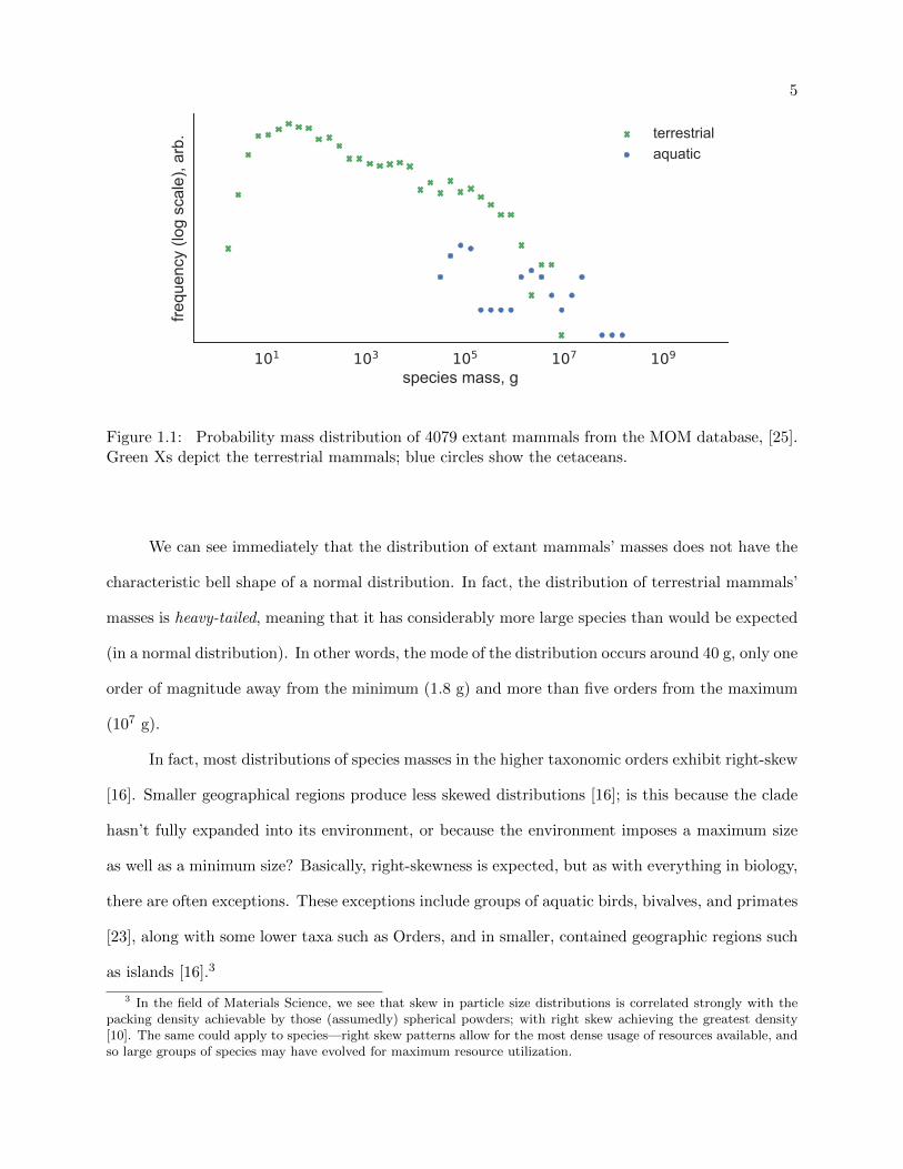
Figure 1.1 depicts the distribution of 4079 mammals’ masses from the late Quaternary (from
MOM, [25]); the horizontal axis shows mass, which was broken up into “bins” (on a log scale), and
the vertical axis shows the relative probability (also on a log scale) of picking a mass in a given bin.
In this way we are looking at a probability distribution, but instead of absolute probabilities—how
likely it is that we choose a mammal of mass x—we are only concerned with relative probabilities—
how much more likely we are to choose a mammal of mass x than one of mass y.
2 Hopefully the idea that our bodies are less complex than those of hippopotamuses is a gentle enough blow toour egos that we can proceed under our mass-as-complexity assumption.
5
101 103 105 107 109
species mass, g
frequ
ency
(log
sca
le),
arb. terrestrial
aquatic
Figure 1.1: Probability mass distribution of 4079 extant mammals from the MOM database, [25].Green Xs depict the terrestrial mammals; blue circles show the cetaceans.
We can see immediately that the distribution of extant mammals’ masses does not have the
characteristic bell shape of a normal distribution. In fact, the distribution of terrestrial mammals’
masses is heavy-tailed, meaning that it has considerably more large species than would be expected
(in a normal distribution). In other words, the mode of the distribution occurs around 40 g, only one
order of magnitude away from the minimum (1.8 g) and more than five orders from the maximum
(107 g).
In fact, most distributions of species masses in the higher taxonomic orders exhibit right-skew
[16]. Smaller geographical regions produce less skewed distributions [16]; is this because the clade
hasn’t fully expanded into its environment, or because the environment imposes a maximum size
as well as a minimum size? Basically, right-skewness is expected, but as with everything in biology,
there are often exceptions. These exceptions include groups of aquatic birds, bivalves, and primates
[23], along with some lower taxa such as Orders, and in smaller, contained geographic regions such
as islands [16].3
3 In the field of Materials Science, we see that skew in particle size distributions is correlated strongly with thepacking density achievable by those (assumedly) spherical powders; with right skew achieving the greatest density[10]. The same could apply to species—right skew patterns allow for the most dense usage of resources available, andso large groups of species may have evolved for maximum resource utilization.

6
Now the question arises: What processes and trends inherent in macroevolution combine to
generate a right-skewed distribution of masses? Our next chapter will discuss these processes and
trends, and use them to build a baseline generative computer model capable of evolving clades with
right-skewed mass distributions.

Chapter 2
Generative Statistical Modeling
When studying (organic) phenomena, it is natural to develop hypotheses that describe the
underlying processes. However, it is often the case that these hypotheses cannot be evaluated
directly, which could happen for any number of reasons. For example, in our investigation we are
unable to directly measure our hypotheses due to the sheer complexity, and notably non-human
time-scale, of macroevolution. Thus the question arises: How can we confirm or deny the validity
of our hypotheses if we are incapable of providing adequate control over the environment to test
them directly?
Enter scientific computation. By using a computer to run simulations built on our hypotheses,
we can check to see whether or not the simulation’s results are indistinguishable from the data we can
measure. If the results do end up being indistinguishable from the data, then we can conclude that
our set of hypotheses constitutes one possible explanation of the phenomenon, and then continue
to test for further dimensions of fit. Along the way, the evidence we collect may help to corroborate
our hypothesis (further showing that our guess was a good one), or it may help us see where our
model differs from reality—either way, what we learn is valuable information about the model and
how it relates to reality.
Note here that we will be modeling effective processes. Obviously there are an astronomical
number of steps involved in the emergence of a new species, but here we consider all those steps to
be collectively approximated through random draws from empirically measured distributions. This
condensation of processes into a single, probabilistic step is critical for creating this model since we
8
do not know how all the underlying steps intertwine, and even if we did know for certain all the
factors that contribute to speciation and how they interact, simulating all of them together would
(currently) be prohibitively computationally expensive.
There are many classes of statistical models, but we will focus here on random walks, as they
are the most natural choice in modeling evolution.
2.1 Random Walk
Evolution is a natural candidate for random walk modeling. In fact, in 1977 Raup [21]
performed a random walk computer simulation of cladogenesis and found that even some large
extinction events, previously thought to be the result of massive one-time ecological changes, could
emerge from random walks.
Named for the fact that each next step in the model is determined independently by a draw
from a distribution, random walk models are characterized by their non-deterministic behavior.
This gives random walks an important property: they have neither memory nor intention—the
direction and magnitude of every step is taken independently of previous and next steps. Thus
location is the only quality of the walker preserved between steps.
Synthesizing the properties of a random walk, we can see that they are an appropriate
approximation of stochastic incremental changes. This follows from the fact that a walker’s position
after taking a step is more dependent on where it was stepping from than how far it stepped. Take
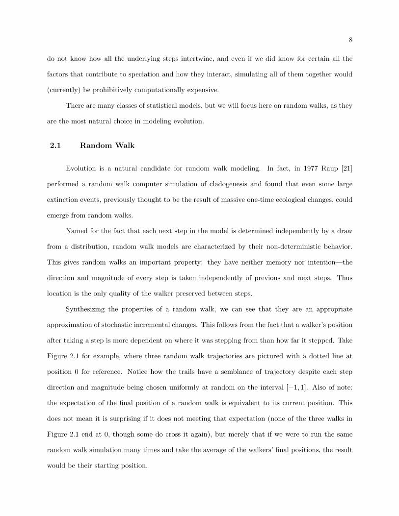
Figure 2.1 for example, where three random walk trajectories are pictured with a dotted line at
position 0 for reference. Notice how the trails have a semblance of trajectory despite each step
direction and magnitude being chosen uniformly at random on the interval [−1, 1]. Also of note:
the expectation of the final position of a random walk is equivalent to its current position. This
does not mean it is surprising if it does not meeting that expectation (none of the three walks in
Figure 2.1 end at 0, though some do cross it again), but merely that if we were to run the same
random walk simulation many times and take the average of the walkers’ final positions, the result
would be their starting position.
9
iteration
posi
tion,
arb
.
Figure 2.1: A collection of three random walks. Step magnitudes (and directions) were generatedby taking a draw from a uniform distribution ranging on the interval [−1, 1]. New positions werecalculated by addition.
101102103
mas
s, g
101102103
mas
s, g
model time
101102103
mas
s, g
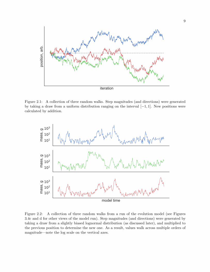
Figure 2.2: A collection of three random walks from a run of the evolution model (see Figures3.4c and d for other views of the model run). Step magnitudes (and directions) were generated bytaking a draw from a slightly biased lognormal distribution (as discussed later), and multiplied tothe previous position to determine the new one. As a result, values walk across multiple orders ofmagnitude—note the log scale on the vertical axes.

10
Figure 2.2 shows random walks taken from a run of the simulation that we will discuss later,
in Section 3.3.1. The paths depict fluctuations in the masses of the chosen species’ ancestors; the
ultimate point on the trajectory is the mass of that species upon simulation termination. (Notice
how the top and bottom species have the same mass lineage up until the final quarter of the
simulation time, when their most recent common ancestor went extinct.) Despite our generating
species masses through a multiplicative factor—mass differences are measured in percentages, not
absolute values—the walks have the same properties as before, just over a log scale instead of a
linear one.
As the fossil record shows, characteristics of species evolve incrementally over time and in
undetermined (if slightly biased) directions. That is to say that the characteristics of a given species
will not differ greatly from those of its direct ancestor, especially when compared to differences
between other lineages. In fact, before genome sequencing was ubiquitous and inexpensive enough to
give us more direct insight on genetic lineages, species relationships were determined by comparing
differences with others: more similarities denoted closer relationships.
2.2 The Clauset-Erwin Model
Now that we have established that the use of a random walk is appropriate for modeling
evolution of a particular species, we need to expand the random walk to simulate the evolution of
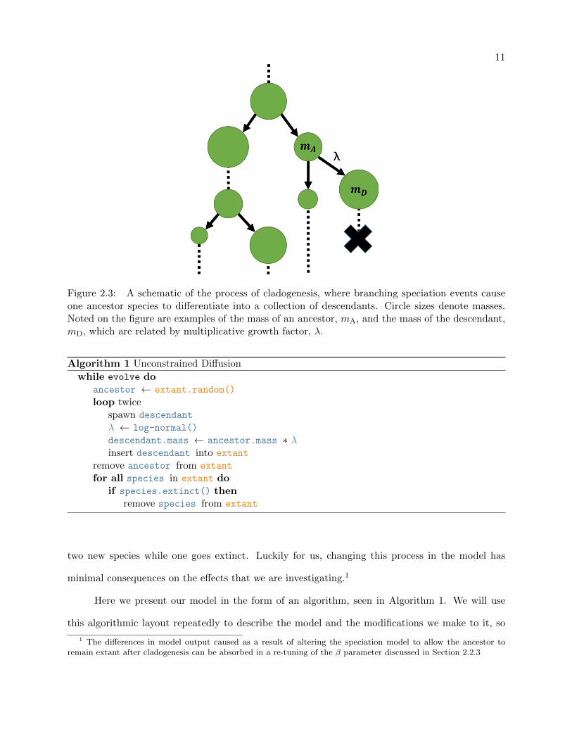
an entire clade. The first step is to implement the branching process inherent in cladogenesis—
depicted schematically in Figure 2.3—to the model. We choose to model speciation events as purely
bifurcating processes, resulting in two descendants (both with novel masses), and the extinction
of the ancestor species. To keep our simulation simple, one cladogenesis event occurs at every
time step of our discrete time model. As a result, our model time has a complicated relationship
with real time that is not in the scope of this thesis but which has been investigated (in [22], for
example).
Obviously, there are many ways that speciation can occur—take allopatric speciation, peripa-
tric speciation, and sympatric speciation for example—and not all have the signature of spawning
11
Figure 2.3: A schematic of the process of cladogenesis, where branching speciation events causeone ancestor species to differentiate into a collection of descendants. Circle sizes denote masses.Noted on the figure are examples of the mass of an ancestor, mA, and the mass of the descendant,mD, which are related by multiplicative growth factor, λ.
Algorithm 1 Unconstrained Diffusion
while evolve doancestor ← extant.random()
loop twicespawn descendant
λ ← log-normal()
descendant.mass ← ancestor.mass ∗ λinsert descendant into extant
remove ancestor from extant
for all species in extant doif species.extinct() then
remove species from extant
two new species while one goes extinct. Luckily for us, changing this process in the model has
minimal consequences on the effects that we are investigating.1
Here we present our model in the form of an algorithm, seen in Algorithm 1. We will use
this algorithmic layout repeatedly to describe the model and the modifications we make to it, so
1 The differences in model output caused as a result of altering the speciation model to allow the ancestor toremain extant after cladogenesis can be absorbed in a re-tuning of the β parameter discussed in Section 2.2.3

12
let us first walk through the most basic version. We will be running the described process at
every cladogenesis step, noted in the algorithm as “while evolve.” In reality, the total number
of cladogenesis steps, tmax, is decided as a function of two fossil record estimates—mean species
lifespan, ν = 1.6 My, and total model time, τ = 250 My since the mammal clade began—and the
expected number of species alive at simulation termination, n, estimated by extant species count.
This results in tmax = τ νn.
The first step in the cladogenesis model is to choose the ancestor uniformly at random from
our set of extant species. Note: for convenience, variables (ancestor) and collections (extant)
in the algorithms are highlighted denoted with blue and orange, respectively. After choosing the
progenitor, we spawn two descendant species and assign them masses mD = λ ∗ mA, where
λ is drawn from a balanced log-normal distribution (〈log(λ)〉 = 0) at random to represent the
descent with variability inherent in evolution. The parameters of the log-normal distribution were
estimated from the fossil record by Clauset and Erwin in [8] and used here without alteration.
After spawning each descendant species, we put both of them in the extant pool, then remove
the ancestor since, under the assumptions of our model, it has gone extinct in the process of
cladogenesis.
Finally, we enter the extinction step where we determine whether any species have gone
extinct due to non-cladogenesis factors. To do so, we iterate through all species and check to see
if they have gone extinct. species.extinct() abstracts this process in Algorithm 1; behind the
scenes, this decision function simply replies with some probability pext = 1/n that the species has
gone extinct. (To speed up the process of iterating through thousands of species with every model
time step, we use the properties of a geometric distribution to pre-determine how many trials we
would have had to perform, without actually performing them. For more information, see Appendix
B.)
Considering we perform cladogenesis and extinction with every step, our model approaches
an equilibrium species count of n after about n steps. Every speciation step creates two new
species (descendants), and causes the ancestor to go extinct; every extinction step will kill off an
13
expected ns/n species (ns tries at pext = 1/n), where ns is the number of species alive at that time.
Thus when ns = n we will expect one extinction per model step, balancing our net speciation and
extinction rates overall and making n a stable attractor for species count.
Under this simple model, the distribution of species masses diffuses over time to fill the
available “space.” We can imagine that species in nature do the same: say a mammal finds its way
to an island where there are no other mammals yet, we would expect that, over evolutionary time,
our exploratory mammal would give rise to a entire clade of diverse (diffuse) mammals species that
find ways to leverage their diversity and take advantage of ecological peculiarities. In this sense, we
are abstracting away a number of ecological factors into the random walk processes of our model.
101 103 105 107 109
species mass, g
frequ
ency
(log
sca
le),
arb. MOM terrestrial
basic
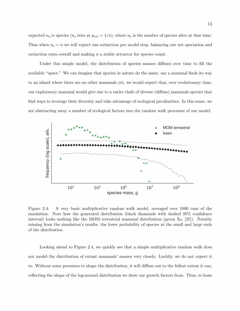
Figure 2.4: A very basic multiplicative random walk model, averaged over 1000 runs of thesimulation. Note how the generated distribution (black diamonds with dashed 95% confidenceinterval) looks nothing like the MOM terrestrial mammal distribution (green Xs, [25]). Notablymissing from the simulation’s results: the lower probability of species at the small and large endsof the distribution.
Looking ahead to Figure 2.4, we quickly see that a simple multiplicative random walk does
not model the distribution of extant mammals’ masses very closely. Luckily, we do not expect it
to. Without some pressures to shape the distribution, it will diffuse out to the fullest extent it can,
reflecting the shape of the log-normal distribution we drew our growth factors from. Thus, to hone
14
the model we need to distill ecological factors—individuals, populations, location, range, niches,
predation, adaptation, and others—into some constraints that will influence the shape of our fully
developed diffusion model.
2.2.1 Adding a Lower Limit
Terrestrial mammals exhibit a lower mass limit. While this fact might not be surprising, it
is an important one; especially because we need to have a model that adheres to this observed con-
straint. However, before we implement our minimum size constraint, let us examine why mammals
can only be so small.
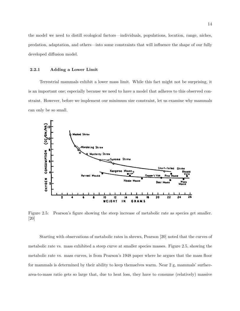
Figure 2.5: Pearson’s figure showing the steep increase of metabolic rate as species get smaller.[20]
Starting with observations of metabolic rates in shrews, Pearson [20] noted that the curves of
metabolic rate vs. mass exhibited a steep curve at smaller species masses. Figure 2.5, showing the
metabolic rate vs. mass curves, is from Pearson’s 1948 paper where he argues that the mass floor
for mammals is determined by their ability to keep themselves warm. Near 2 g, mammals’ surface-
area-to-mass ratio gets so large that, due to heat loss, they have to consume (relatively) massive

15
amounts of food to satisfy their metabolism and sustain their body temperature. Unsurprisingly,
the smallest mammal known to be alive today (Remy’s Pygmy Shrew, 1.8 g) lives in the tropical
forests of central Africa; the consistently warm temperatures there are likely what allow Remy’s
Pygmy Shrew to survive at such a small mass.
Algorithm 2 Diffusion with Lower Limit
while evolve doancestor ← extant.random()
loop twicespawn descendant
repeatλ ← log-normal()
descendant.mass ← ancestor.mass ∗ λuntil descendant.mass ≥ mmin
insert descendant into extant
remove ancestor from extant
for all species in extant doif species.extinct() then
remove species from extant
To add this lower limit to our simulation, we add in a check when drawing the growth
factor, λ, from a log-normal distribution. As seen in Algorithm 2, we simply disallow λ values
that would cause the new descendant’s mass to drop below the minimum size, mmin, and redraw
until we find a λ that satisfies our constraint. In a study of diffusion this lower limit would be
considered a reflecting boundary, causing species that would have crossed it to “reflect” back into
the distribution’s bulk.
The results of adding a minimum size boundary of 1.8 g to the model can be seen in Figure
2.6. Notice the downward bend in the distribution near 100 g, our model’s minimum mass, which
also has the effect of moving the mode from the minimum to a point just above the minimum.
Adding a minimum size boundary does not serve to fully specify our model yet, though; we still
need to add constraints for two other empirical trends.
16
101 103 105 107 109
species mass, g
frequ
ency
(log
sca
le),
arb. MOM terrestrial
min
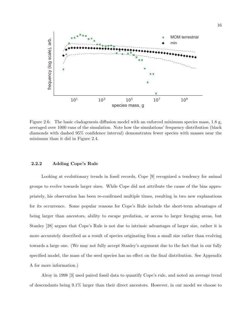
Figure 2.6: The basic cladogenesis diffusion model with an enforced minimum species mass, 1.8 g,averaged over 1000 runs of the simulation. Note how the simulations’ frequency distribution (blackdiamonds with dashed 95% confidence interval) demonstrates fewer species with masses near theminimum than it did in Figure 2.4.
2.2.2 Adding Cope’s Rule
Looking at evolutionary trends in fossil records, Cope [9] recognized a tendency for animal
groups to evolve towards larger sizes. While Cope did not attribute the cause of the bias appro-
priately, his observation has been re-confirmed multiple times, resulting in two new explanations
for its occurrence. Some popular reasons for Cope’s Rule include the short-term advantages of
being larger than ancestors, ability to escape predation, or access to larger foraging areas, but
Stanley [28] argues that Cope’s Rule is not due to intrinsic advantages of larger size, rather it is
more accurately described as a result of species originating from a small size rather than evolving
towards a large one. (We may not fully accept Stanley’s argument due to the fact that in our fully
specified model, the mass of the seed species has no effect on the final distribution. See Appendix
A for more information.)
Alroy in 1998 [3] used paired fossil data to quantify Cope’s rule, and noted an average trend
of descendants being 9.1% larger than their direct ancestors. However, in our model we choose to
17
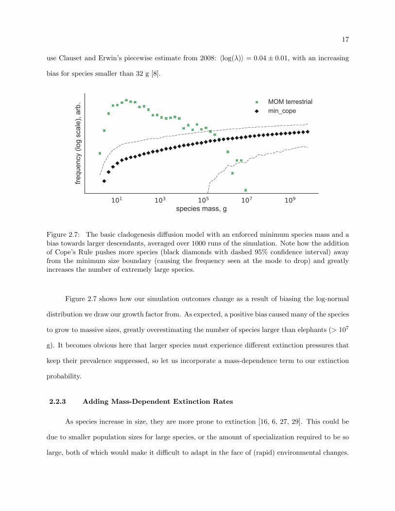
use Clauset and Erwin’s piecewise estimate from 2008: 〈log(λ)〉 = 0.04 ± 0.01, with an increasing
bias for species smaller than 32 g [8].
101 103 105 107 109
species mass, g
frequ
ency
(log
sca
le),
arb. MOM terrestrial
min_cope
Figure 2.7: The basic cladogenesis diffusion model with an enforced minimum species mass and abias towards larger descendants, averaged over 1000 runs of the simulation. Note how the additionof Cope’s Rule pushes more species (black diamonds with dashed 95% confidence interval) awayfrom the minimum size boundary (causing the frequency seen at the mode to drop) and greatlyincreases the number of extremely large species.
Figure 2.7 shows how our simulation outcomes change as a result of biasing the log-normal
distribution we draw our growth factor from. As expected, a positive bias caused many of the species
to grow to massive sizes, greatly overestimating the number of species larger than elephants (> 107
g). It becomes obvious here that larger species must experience different extinction pressures that
keep their prevalence suppressed, so let us incorporate a mass-dependence term to our extinction
probability.
2.2.3 Adding Mass-Dependent Extinction Rates
As species increase in size, they are more prone to extinction [16, 6, 27, 29]. This could be
due to smaller population sizes for large species, or the amount of specialization required to be so
large, both of which would make it difficult to adapt in the face of (rapid) environmental changes.
18
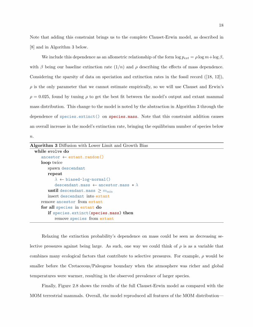
Note that adding this constraint brings us to the complete Clauset-Erwin model, as described in
[8] and in Algorithm 3 below.
We include this dependence as an allometric relationship of the form log pext = ρ logm+log β,
with β being our baseline extinction rate (1/n) and ρ describing the effects of mass dependence.
Considering the sparsity of data on speciation and extinction rates in the fossil record ([18, 12]),
ρ is the only parameter that we cannot estimate empirically, so we will use Clauset and Erwin’s
ρ = 0.025, found by tuning ρ to get the best fit between the model’s output and extant mammal
mass distribution. This change to the model is noted by the abstraction in Algorithm 3 through the
dependence of species.extinct() on species.mass. Note that this constraint addition causes
an overall increase in the model’s extinction rate, bringing the equilibrium number of species below
n.
Algorithm 3 Diffusion with Lower Limit and Growth Bias
while evolve doancestor ← extant.random()
loop twicespawn descendant
repeatλ ← biased-log-normal()
descendant.mass ← ancestor.mass ∗ λuntil descendant.mass ≥ mmin
insert descendant into extant
remove ancestor from extant
for all species in extant doif species.extinct(species.mass) then
remove species from extant
Relaxing the extinction probability’s dependence on mass could be seen as decreasing se-
lective pressures against being large. As such, one way we could think of ρ is as a variable that
combines many ecological factors that contribute to selective pressures. For example, ρ would be
smaller before the Cretaceous/Paleogene boundary when the atmosphere was richer and global
temperatures were warmer, resulting in the observed prevalence of larger species.
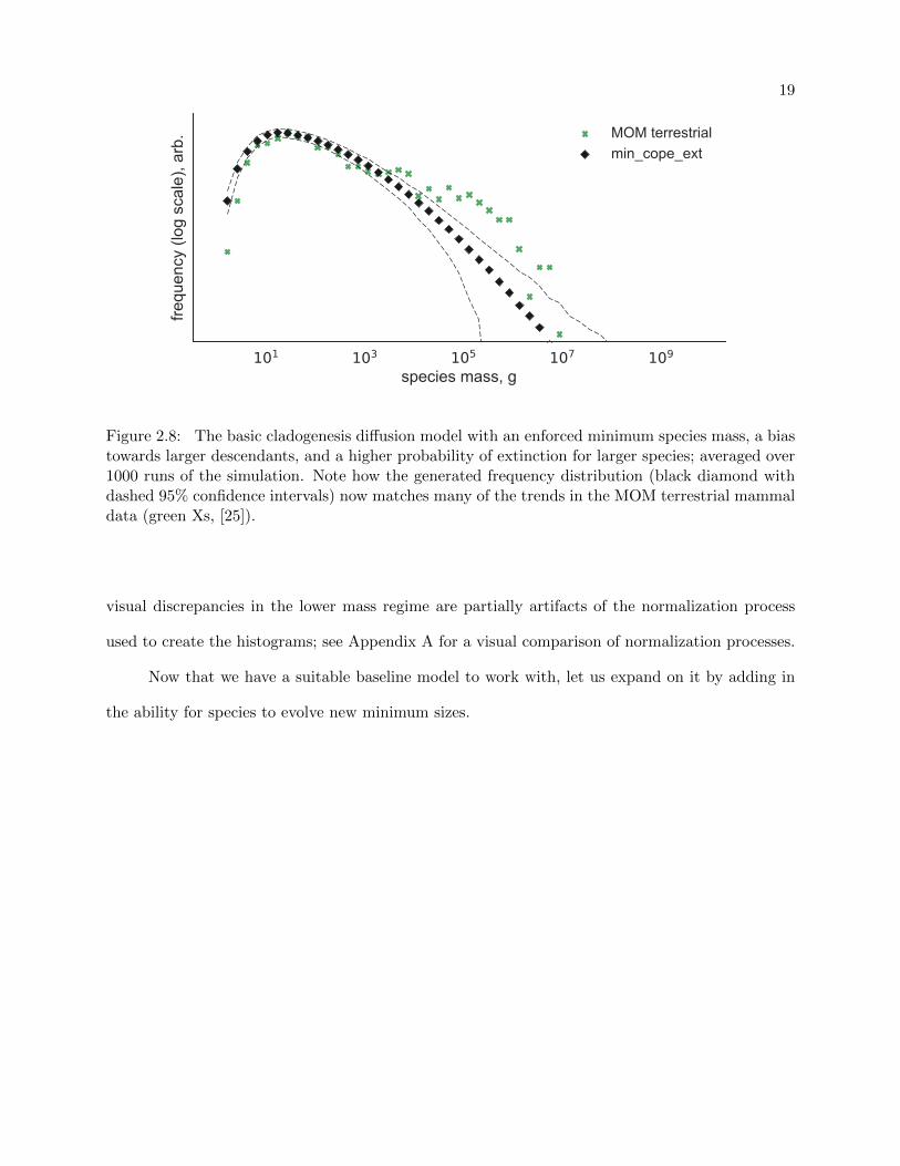
Finally, Figure 2.8 shows the results of the full Clauset-Erwin model as compared with the
MOM terrestrial mammals. Overall, the model reproduced all features of the MOM distribution—
19
101 103 105 107 109
species mass, g
frequ
ency
(log
sca
le),
arb. MOM terrestrial
min_cope_ext
Figure 2.8: The basic cladogenesis diffusion model with an enforced minimum species mass, a biastowards larger descendants, and a higher probability of extinction for larger species; averaged over1000 runs of the simulation. Note how the generated frequency distribution (black diamond withdashed 95% confidence intervals) now matches many of the trends in the MOM terrestrial mammaldata (green Xs, [25]).
visual discrepancies in the lower mass regime are partially artifacts of the normalization process
used to create the histograms; see Appendix A for a visual comparison of normalization processes.
Now that we have a suitable baseline model to work with, let us expand on it by adding in
the ability for species to evolve new minimum sizes.
Chapter 3
Propagating Ratchets
As the complexity of a species follows its random walk, there comes a possibility that an
evolved characteristic provides some implicit advantage. Along with that advantage, let us also say
that the increase in complexity has made it impossible to be smaller than a certain size—that the
advantage has raised the floor for how small any descendants could be. For convenience, we will
name occurrences of these innovative (effectively) irreversible increases in complexity ratchets.
There are many examples of ratchets in evolution. For example, when eukaryotes emerged
from prokaryotes the range of abilities of the organisms increased but at the cost of having a
larger minimum size—each eukaryote has to be at least large enough to fit a nucleus and mito-
chondria, features their ancestral prokaryotes did not possess. For another example, we can fast
forward roughly two billion years from the first of the eukaryotes to the emergence of mammals,
whose minimum size is determined by a complicated combination of evolved traits that resulted in
endothermy.
3.1 Identifying Ratchets
Ratchets, and their resulting mass floors, are quite difficult to identify. For example, let us
examine a sub-clade of mammals: the canines. What is the minimum size of a canine? We could
look for the smallest adult canine known to exist—as a result of our artificial selection, this figure is
currently just under 700 g (about 1.5 lbs) [26]—but how do we know that it is the smallest dog that
could exist? Short answer: We do not (but it is probably a good estimate). Currently, determining
21
the minimum size of a clade requires that the clade be large enough to have fully expanded to its
viable size boundary, giving us empirical data to draw from like we did in determining the minimum
size for terrestrial mammals by taking the smallest known mammal, Remy’s Pygmy Shrew at 1.8
g, as our minimum terrestrial mammal size.
101 103 105 107 109
species mass, g
frequ
ency
(log
sca
le),
arb. terrestrial
aquatic
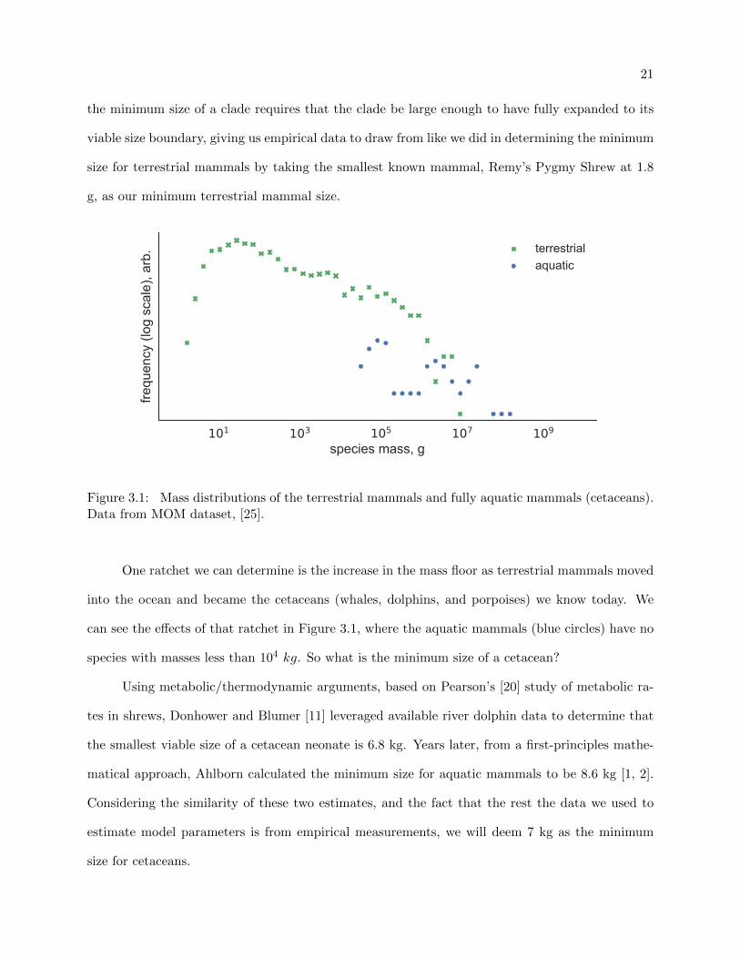
Figure 3.1: Mass distributions of the terrestrial mammals and fully aquatic mammals (cetaceans).Data from MOM dataset, [25].
One ratchet we can determine is the increase in the mass floor as terrestrial mammals moved
into the ocean and became the cetaceans (whales, dolphins, and porpoises) we know today. We
can see the effects of that ratchet in Figure 3.1, where the aquatic mammals (blue circles) have no
species with masses less than 104 kg. So what is the minimum size of a cetacean?
Using metabolic/thermodynamic arguments, based on Pearson’s [20] study of metabolic ra-
tes in shrews, Donhower and Blumer [11] leveraged available river dolphin data to determine that
the smallest viable size of a cetacean neonate is 6.8 kg. Years later, from a first-principles mathe-
matical approach, Ahlborn calculated the minimum size for aquatic mammals to be 8.6 kg [1, 2].
Considering the similarity of these two estimates, and the fact that the rest the data we used to
estimate model parameters is from empirical measurements, we will deem 7 kg as the minimum
size for cetaceans.
22Algorithm 4 Adding an Inheritable, Ratcheting Minimum Size
while evolve doancestor ← extant.random()
loop twicespawn descendant
repeatλ ← biased-log-normal()
descendant.mass ← ancestor.mass ∗ λuntil descendant.mass ≥ ancestor.min
if ratchet() thendescendant.min ← descendant.mass
elsedescendant.min ← ancestor.min
insert descendant into extant
remove ancestor from extant
for all species in extant doif species.extinct(mass) then remove species from extant
Clauset [7] has already employed our estimate of a cetacean mass floor by updating only the
minimum size parameter of the simulation described in Section 2.2.3 to create a version that simu-
lates aquatic mammals. Remarkably, the results of the cetacean model revealed that by changing
only the minimum size, and leaving all other parameters as estimated for terrestrial mammals, spe-
cies as large as blue whales became likely! In other words, raising the hard minimum size boundary
increases the pressure towards higher masses pushing the maximum likely mass deeper into the
passive pressures of mass-dependent extinction.
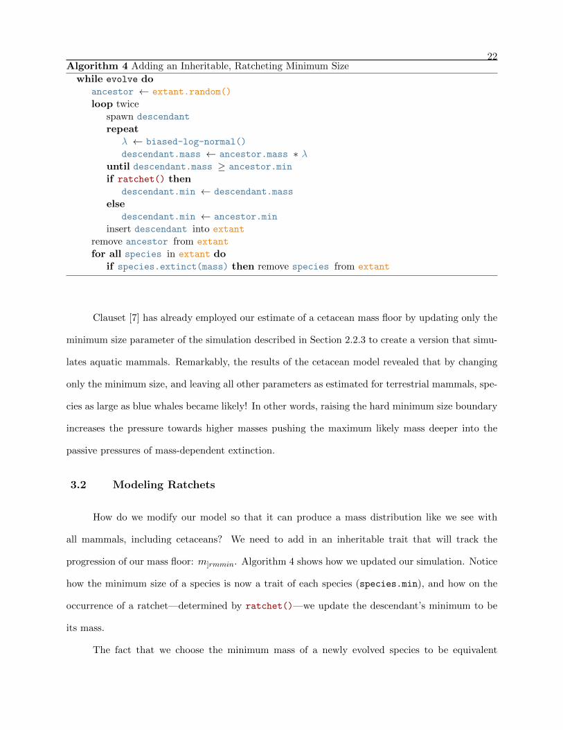
3.2 Modeling Ratchets
How do we modify our model so that it can produce a mass distribution like we see with
all mammals, including cetaceans? We need to add in an inheritable trait that will track the
progression of our mass floor: m]rmmin. Algorithm 4 shows how we updated our simulation. Notice
how the minimum size of a species is now a trait of each species (species.min), and how on the
occurrence of a ratchet—determined by ratchet()—we update the descendant’s minimum to be
its mass.
The fact that we choose the minimum mass of a newly evolved species to be equivalent

23
to its current mass follows the logical upper bound of the problem: a species of mass m must
have a minimum mass mmin such that mmin ≤ m. We can also identify a lower bound to our
new species’ minimum size in the ancestor’s mmin, giving us a viable range of minimum sizes
from mmin,A ≤ mmin,D ≤ mD, where the A and D subscripts denote ancestor and descendant,
respectively. We opt to take the maximum of this range because the mass of the first species in the
clade does not affect the qualities of the resulting equilibrium distribution. Thus, by the assumption
that the mmin of concern would have evolved regardless, we can choose to take the maximum for
convenience. (Also, the differences induced in the model by choosing an mmin,D other than than
mD are not significant enough to change the qualitative behavior of the model and therefore do not
warrant deviating from convenience.)
Another large change to the model is the addition of the ratchet() decision function, seen
in Algorithm 4. This function performs a simple probabilistic decision: with some probability, pr,
the function will return true. In short, we are implementing ratchets under the assumption that
the chance a ratchet occurs is independent from all other factors, and constant for all species.
Now we encounter a difficult question: How often do ratchets occur? Answers to this question
could span many orders of magnitude, from “every time a new feature evolves,” pr = 1, to “only
when factors are just right,” which could make pr < 10−6, less than one in a million. In fact, owing
to the difficulty of determining different mass floors, making an estimation of ratchet prevalence
from (sparse) fossil records is currently nigh impossible. Thus we will investigate different ratchet
probabilities in the following sections, where appropriate, and the probabilities will generally be
in the range 10−6 < pr < 10−3, because higher probabilities can cause the model to “run away”
and evolve species of inconceivable masses. Unless otherwise specified, we will use pr = 1/20000 to
get a good balance between ratchet prevalence without overloading the model. Note that despite
not being able to estimate pr, we still find value in experimenting with the model as a means of
building intuition, which we do through the careful numerical experiments that follow.
24
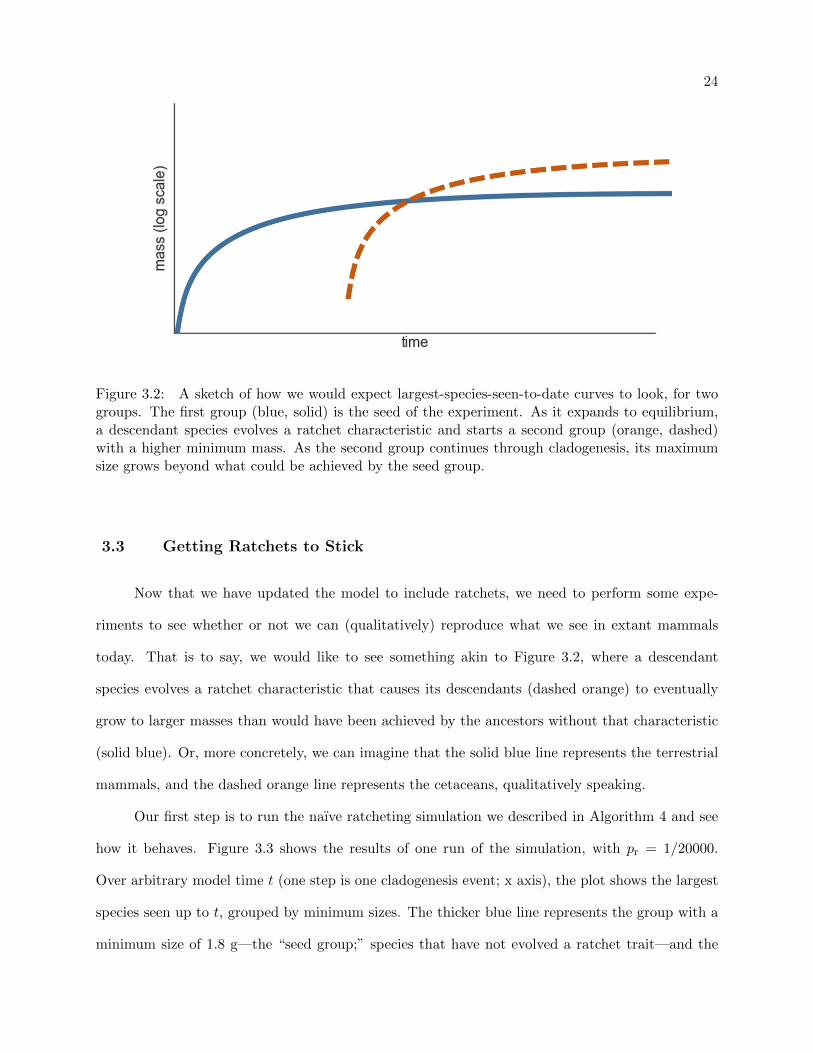
Figure 3.2: A sketch of how we would expect largest-species-seen-to-date curves to look, for twogroups. The first group (blue, solid) is the seed of the experiment. As it expands to equilibrium,a descendant species evolves a ratchet characteristic and starts a second group (orange, dashed)with a higher minimum mass. As the second group continues through cladogenesis, its maximumsize grows beyond what could be achieved by the seed group.
3.3 Getting Ratchets to Stick
Now that we have updated the model to include ratchets, we need to perform some expe-
riments to see whether or not we can (qualitatively) reproduce what we see in extant mammals
today. That is to say, we would like to see something akin to Figure 3.2, where a descendant
species evolves a ratchet characteristic that causes its descendants (dashed orange) to eventually
grow to larger masses than would have been achieved by the ancestors without that characteristic
(solid blue). Or, more concretely, we can imagine that the solid blue line represents the terrestrial
mammals, and the dashed orange line represents the cetaceans, qualitatively speaking.
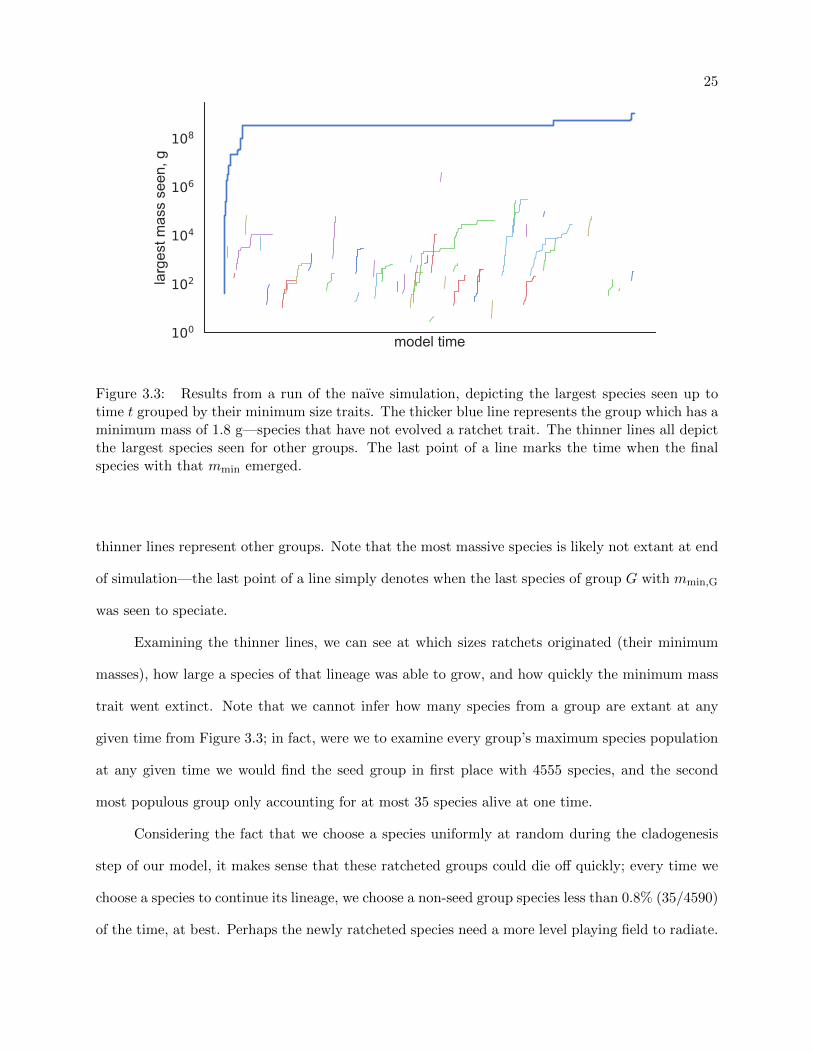
Our first step is to run the naıve ratcheting simulation we described in Algorithm 4 and see
how it behaves. Figure 3.3 shows the results of one run of the simulation, with pr = 1/20000.
Over arbitrary model time t (one step is one cladogenesis event; x axis), the plot shows the largest
species seen up to t, grouped by minimum sizes. The thicker blue line represents the group with a
minimum size of 1.8 g—the “seed group;” species that have not evolved a ratchet trait—and the
25
model time100
102
104
106
108
larg
est m
ass
seen
, g
Figure 3.3: Results from a run of the naıve simulation, depicting the largest species seen up totime t grouped by their minimum size traits. The thicker blue line represents the group which has aminimum mass of 1.8 g—species that have not evolved a ratchet trait. The thinner lines all depictthe largest species seen for other groups. The last point of a line marks the time when the finalspecies with that mmin emerged.
thinner lines represent other groups. Note that the most massive species is likely not extant at end
of simulation—the last point of a line simply denotes when the last species of group G with mmin,G
was seen to speciate.
Examining the thinner lines, we can see at which sizes ratchets originated (their minimum
masses), how large a species of that lineage was able to grow, and how quickly the minimum mass
trait went extinct. Note that we cannot infer how many species from a group are extant at any
given time from Figure 3.3; in fact, were we to examine every group’s maximum species population
at any given time we would find the seed group in first place with 4555 species, and the second
most populous group only accounting for at most 35 species alive at one time.
Considering the fact that we choose a species uniformly at random during the cladogenesis
step of our model, it makes sense that these ratcheted groups could die off quickly; every time we
choose a species to continue its lineage, we choose a non-seed group species less than 0.8% (35/4590)
of the time, at best. Perhaps the newly ratcheted species need a more level playing field to radiate.
26
To give the newly ratcheted species this fighting chance to thrive, we will perform experiments
to perturb the balance of species and see if there are any conditions under which we see what we
have predicted in Figure 3.2. After all, it is entirely possible that certain perturbation events
need to occur for new ratchets to find their ecological foothold and radiate—many argue that the
extinction of the dinosaurs at the Cretaceous/Paleogene (K/Pg) boundary is what opened up the
space for the radiation of mammals [24].
3.3.1 Dropping Meteors
Our first method of perturbing the system involves a massive extinction event, ostensibly
caused by a meteor. However, more generally, we can imagine this perturbation to be a global
change—whether it is due to a shift in climate, massive volcanic eruption, runaway greenhouse
effect, or the impact of an enormous rock.
We simulate the impact of a meteor by choosing a timestep halfway through the simulation
when the event will occur. When that timestep occurs in the simulation, we iterate over all species
that are extant and kill them off with some probability of extinction by meteor, pebm. Figure 3.4a
shows the effect of dropping a meteor halfway through a run of the naıve simulation—killing off
species with a pebm = 0.5 and making 2256 of 4501 go extinct—through the largest-species-seen
lens. Referring back to Figure 3.3, we can see that there is no real appreciable difference between
the two.
Examining Figure 3.4b—a view of the number of species extant at model time t grouped by
minimum sizes—we can verify that a mass-extinction event took place. (Note: the impact of the
meteor on the seed group, thick blue line, is underrepresented in the figure due to the numerical
integration used to generate the plot.) Figure 3.4b also graphically demonstrates what we discussed
about the naıve model above: populations of ratcheted groups make up less than 2% of the entire
pool of extant species at any given time.
Due to pebm being independent and identical for all species in the last experiment, we made
little to no impact on the relative populations between the seed and ratcheted groups. Thus, to
27
model time
101
103
105
107
109
larg
est m
ass
seen
, ga)
model time
101
103
105
107
109
larg
est m
ass
seen
, g
c)
model time0
1000
2000
3000
4000
num
ber o
f ext
ant s
peci
es, b
y gr
oup b)
model time0
1000
2000
3000
4000
num
ber o
f ext
ant s
peci
es, b
y gr
oup d)
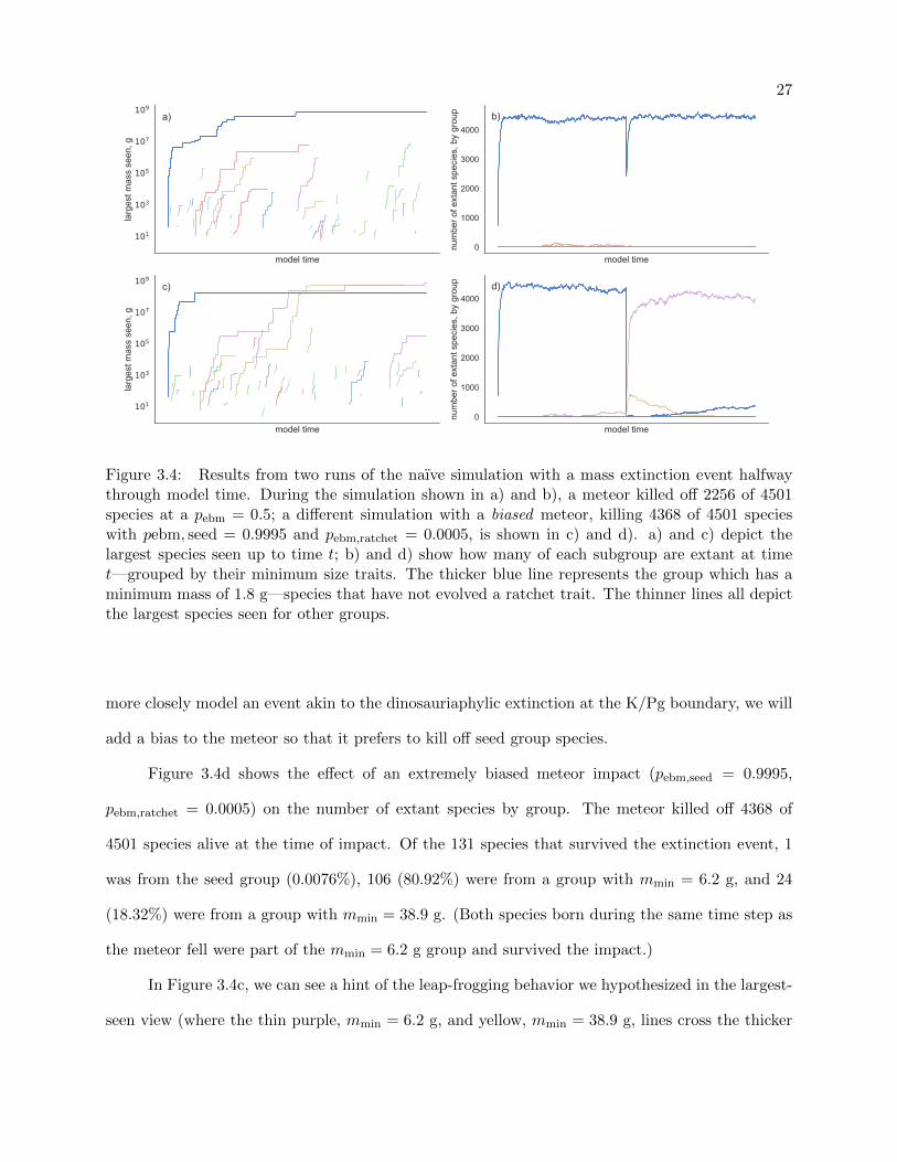
Figure 3.4: Results from two runs of the naıve simulation with a mass extinction event halfwaythrough model time. During the simulation shown in a) and b), a meteor killed off 2256 of 4501species at a pebm = 0.5; a different simulation with a biased meteor, killing 4368 of 4501 specieswith pebm, seed = 0.9995 and pebm,ratchet = 0.0005, is shown in c) and d). a) and c) depict thelargest species seen up to time t; b) and d) show how many of each subgroup are extant at timet—grouped by their minimum size traits. The thicker blue line represents the group which has aminimum mass of 1.8 g—species that have not evolved a ratchet trait. The thinner lines all depictthe largest species seen for other groups.
more closely model an event akin to the dinosauriaphylic extinction at the K/Pg boundary, we will
add a bias to the meteor so that it prefers to kill off seed group species.
Figure 3.4d shows the effect of an extremely biased meteor impact (pebm,seed = 0.9995,
pebm,ratchet = 0.0005) on the number of extant species by group. The meteor killed off 4368 of
4501 species alive at the time of impact. Of the 131 species that survived the extinction event, 1
was from the seed group (0.0076%), 106 (80.92%) were from a group with mmin = 6.2 g, and 24
(18.32%) were from a group with mmin = 38.9 g. (Both species born during the same time step as
the meteor fell were part of the mmin = 6.2 g group and survived the impact.)
In Figure 3.4c, we can see a hint of the leap-frogging behavior we hypothesized in the largest-
seen view (where the thin purple, mmin = 6.2 g, and yellow, mmin = 38.9 g, lines cross the thicker

28
blue one), but upon comparing it to Figure 3.4d it becomes obvious that the behavior is a byproduct
of the near-extinction of the seed group. Thus we have determined that the behavior we expect
can happen as the result of a (heavily) biased mass-extinction event that tips the balance of mmin
frequency out of the seed group’s favor. However, this result does not satisfy the conditions under
which we see cetaceans emerge—the terrestrial mammals have not gone extinct to make way for
the water-dwellers—so we will continue to search for a more general condition.
3.3.2 Radiative Promotion for Recent Ratchets
The second way we will perturb the equilibrium is to give recently ratcheted species a short
phase of preferential radiation. We implement this in the model by choosing only to speciate from
groups that have experienced a ratchet within the last tr model steps. Figure 3.5 shows some results
from two simulations with different tr values. Plots a) and b) in Figure 3.5 are from a run with
tr = 100, and plots c) and d) had tr = 500.
The first item of note in Figures 3.5a and c is the longer time that we see ratcheted groups
survive. Instead of the short-lived ratchet groups we saw in our naıve and meteor models (Figures
3.3 and 3.4), we now have many groups surviving until the present day. In fact, in the simula-
tion with tr = 100, 20 groups remained extant at model termination. It is apparent that giving
recently ratcheted groups a more populous base (and therefore a greater chance of getting chosen
for cladogenesis after the promotion phase) significantly increases their longevity.
Looking at Figure 3.5d, we can easily see the radiative spikes due to the promotion phase,
extending up to a population of 500, then following a trajectory akin to a random walk. Figure
3.5b has a similar pattern, which is harder to distinguish due to the radiative phase in that run of
the simulation only bolstering group populations to 100 before returning to choosing ancestors uni-
formly at random from the extant pool. Despite the more interesting behavior of these simulations,
large promotional phases are not ecologically justifiable without unrealistic assumptions about the
way speciation events over short periods of time are distributed across a diverse ecosystem.
Together, Figures 3.5b and d serve to show how the seed group manages to push other,
29
model time
101
103
105
107
109la
rges
t mas
s se
en, g
a)
model time
101
103
105
107
109
1011
1013
larg
est m
ass
seen
, g
c)
model time0
1000
2000
3000
4000
num
ber o
f ext
ant s
peci
es, b
y gr
oup b)
model time0
500
1000
1500
2000
2500
3000
num
ber o
f ext
ant s
peci
es, b
y gr
oup d)
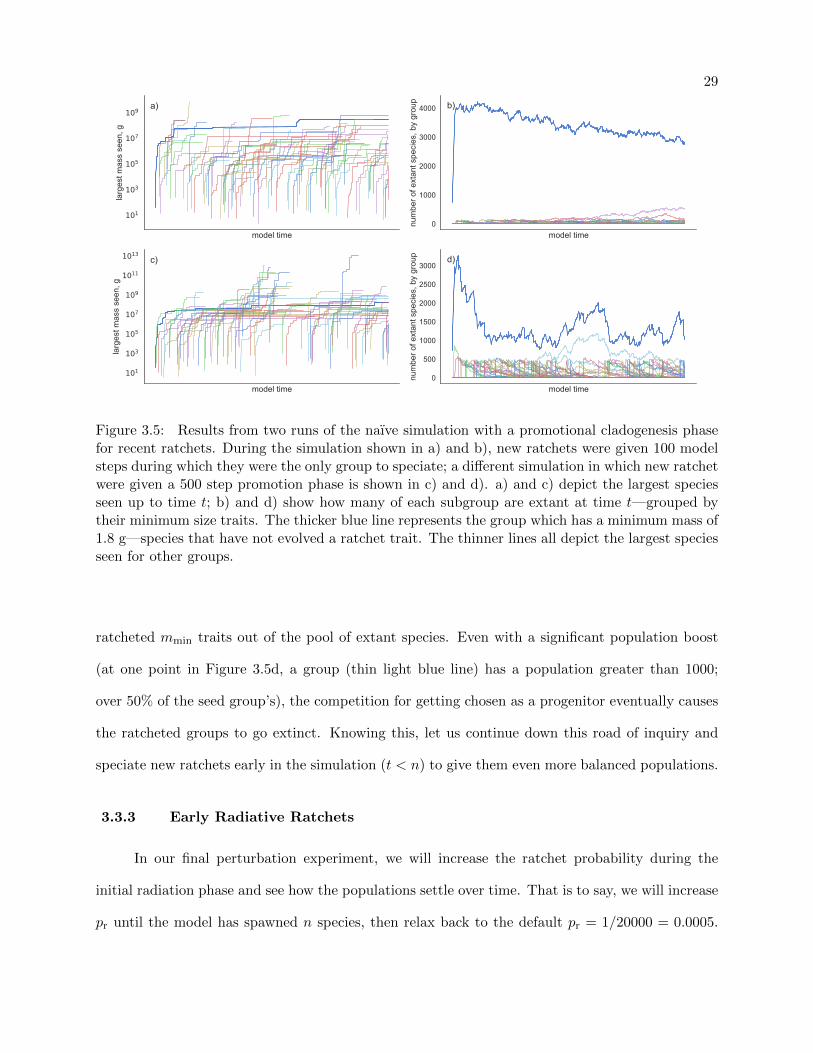
Figure 3.5: Results from two runs of the naıve simulation with a promotional cladogenesis phasefor recent ratchets. During the simulation shown in a) and b), new ratchets were given 100 modelsteps during which they were the only group to speciate; a different simulation in which new ratchetwere given a 500 step promotion phase is shown in c) and d). a) and c) depict the largest speciesseen up to time t; b) and d) show how many of each subgroup are extant at time t—grouped bytheir minimum size traits. The thicker blue line represents the group which has a minimum mass of1.8 g—species that have not evolved a ratchet trait. The thinner lines all depict the largest speciesseen for other groups.
ratcheted mmin traits out of the pool of extant species. Even with a significant population boost
(at one point in Figure 3.5d, a group (thin light blue line) has a population greater than 1000;
over 50% of the seed group’s), the competition for getting chosen as a progenitor eventually causes
the ratcheted groups to go extinct. Knowing this, let us continue down this road of inquiry and
speciate new ratchets early in the simulation (t < n) to give them even more balanced populations.
3.3.3 Early Radiative Ratchets
In our final perturbation experiment, we will increase the ratchet probability during the
initial radiation phase and see how the populations settle over time. That is to say, we will increase
pr until the model has spawned n species, then relax back to the default pr = 1/20000 = 0.0005.
30
model time
101
103
105
107
109
1011
larg
est m
ass
seen
, ga)
model time
102
104
106
108
1010
larg
est m
ass
seen
, g
c)
model time0
1000
2000
3000
4000
num
ber o
f ext
ant s
peci
es, b
y gr
oup b)
model time0
500
1000
1500
2000
2500
3000
3500
num
ber o
f ext
ant s
peci
es, b
y gr
oup d)
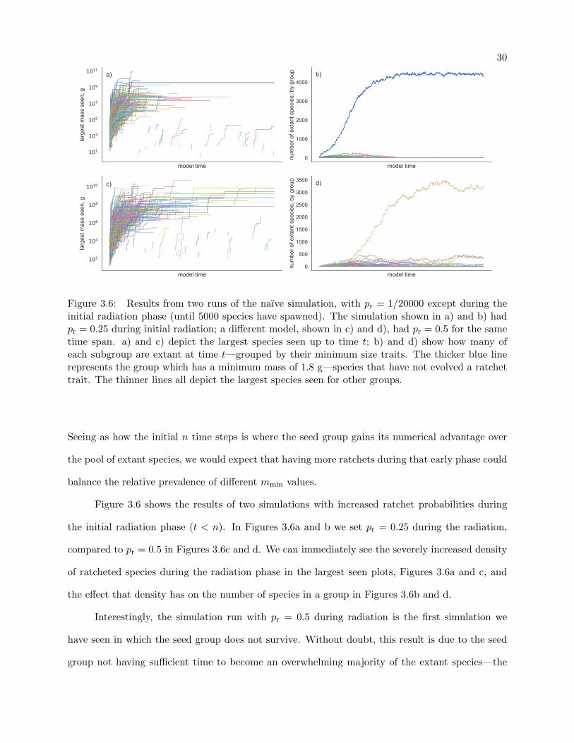
Figure 3.6: Results from two runs of the naıve simulation, with pr = 1/20000 except during theinitial radiation phase (until 5000 species have spawned). The simulation shown in a) and b) hadpr = 0.25 during initial radiation; a different model, shown in c) and d), had pr = 0.5 for the sametime span. a) and c) depict the largest species seen up to time t; b) and d) show how many ofeach subgroup are extant at time t—grouped by their minimum size traits. The thicker blue linerepresents the group which has a minimum mass of 1.8 g—species that have not evolved a ratchettrait. The thinner lines all depict the largest species seen for other groups.
Seeing as how the initial n time steps is where the seed group gains its numerical advantage over
the pool of extant species, we would expect that having more ratchets during that early phase could
balance the relative prevalence of different mmin values.
Figure 3.6 shows the results of two simulations with increased ratchet probabilities during
the initial radiation phase (t < n). In Figures 3.6a and b we set pr = 0.25 during the radiation,
compared to pr = 0.5 in Figures 3.6c and d. We can immediately see the severely increased density
of ratcheted species during the radiation phase in the largest seen plots, Figures 3.6a and c, and
the effect that density has on the number of species in a group in Figures 3.6b and d.
Interestingly, the simulation run with pr = 0.5 during radiation is the first simulation we
have seen in which the seed group does not survive. Without doubt, this result is due to the seed
group not having sufficient time to become an overwhelming majority of the extant species—the

31
first species to spawn from cladogenesis experienced a ratchet, giving the seed group only a 50%
chance of survival by step 2. Compound that with a continued pr = 0.5 and we can see that if the
only remaining seed group is chosen as an ancestor, it is expected that one of its two descendants
will experience a ratchet, reducing the seed group’s prevalence even further.
3.3.4 Discussion
Combined, the above experiments highlight a prevalent theme—the groups seem to be com-
peting for slots in the pool of extant species, occupancy of which correlates strongly with a group’s
longevity. We can see this competition prevalently in Figures 3.5b and d (where the population of
the seed group declines noticeably with every promotional phase), as well as in Figures 3.6d (where
another group takes an early advantage and causes the seed group to go extinct).
Where does this competition come from? We have not included any ostentatious competition
in the model, so it must be an emergent behavior stemming from a choice we made in the design
of our simulation. To understand more, we turn to a method of modeling evolution on a smaller
scale: population genetics.
3.3.5 Population Genetics
Having a species’ minimum size as an inheritable trait—selected for inheritance from a pool
of ancestors uniformly at random—results in competition between sub-populations for dominance
of the pool. Diving into population genetics literature, we can see that this is exactly how we would
expect the prevalence of alleles (variations on a gene) to act in a population. [14]
Note that our model is not the same as ones used in population genetics because we are not
concerned with mating (as that happens on the population level and, by definition, not between
species). In fact, comparing basic population genetics models with ours, we notice that only the
method used to choose an allele (mmin) to inherit is the same: uniformly at random from the
entire population. That similarity alone is enough to cause the behavior we see: due to choosing
inheritance uniformly at random, the probability of a particular trait to saturate a pool becomes

32
equal to the frequency of that allele at a given time. In this way, the survival probability of
beneficial mutations is (approximately) independent of population size, and depends only on the
relative prevalence of the mutation in the population [14].
3.3.6 Genetic Drift vs. Random Mutation
Genetic Drift is the random walk of the prevalence of an allele, which can result in the vanis-
hing of alleles—and therefore reduction in the diversity of the population—throughout generations.
This plays counter to random mutations (descent with variability), which provide new alleles and
increase diversity. [14]
In our model, random mutations come from the ratcheting step: evolved mmin values create
new “alleles” in the pool with probability pr. Genetic drift then occurs due to the process by which
we are choosing ancestors in the cladogenesis step, pushing many of the mutated mmin alleles to
extinction.
Instead of neutral theory, discuss in terms of random walks: drift, extinction,
fixation.This interplay between genetic drift and random mutation is the heart of Neutral The-
ory in Population Genetics, which states that most genetic substitutions are due to genetic drift
pushing other alleles out of the population, not due to the pressures of natural selection. This is
seen as not being at odds with Darwin—the implication of Neutral Theory is simply that most
substitutions have no influence on fitness.
The similarity between our naıve simulation and population genetics brings up a critical
concern: Neutral Theory violates our assumption that ratcheting provides an increase in fitness.
3.4 Conclusions
Given that our simulation is experiencing dynamics similar to those of population genetics—
namely evolution consistent with Neutral Theory—we can conclude that the naıve model we explo-
red in this chapter has a flaw that keeps it from performing as we hypothesized. Implicit competition
in the selection of a progenitor during cladogenesis keeps the species in our model from finding a

33
stable equilibrium with multiple groups living in harmony.
This insight helps us tremendously—in order to see the behavior we hypothesized, we must
prevent the implicit competition between groups.

Chapter 4
Adding Dimensions in Nichespace
When ratcheting traits are treated as alleles in a population, they are reduced to just that:
alleles in a population. However, ratchets are more than that—they provide an advantage to species
which evolve them. Also—as shown in the previous chapter—when a species experiences a ratchet,
it must gain access to a new space where it can diversify without competing with other lineages.
If we reimagine our simulation as starting off with one dimension in niche space, with capacity
for n species, along which a group can optimize or adapt, it becomes obvious how we can expand
our model to mitigate competition between groups—we can add a new dimension of niche space.
In this chapter, we examine how to define that expansion of niche space in the model and then
show that our updated model is capable of producing the desired behavior, as discussed in 3.2.
4.1 Expanding Nichespace
The first question that comes about when adding a dimension to our niche space is “How many
species can it hold?” To answer that question, we need to look at how the sizes of taxonomic groups
scale with their minimum masses. Our available data include three mammal-related groups—
Mammalia [8], Cetacea [7], and Equidae [22]—that have been used in previous studies with the
diffusion model as described in Section 2.2.3. These three groups, along with their associated mmins
and extant species counts are tabulated in Table 4.1.
Canonically, allometric scaling relationships are calculated by fitting a line such that y = kxa,
or in log form, log y = a log x+log k. In our case, we found the coefficients a = −0.6 and log k = 3.8
35
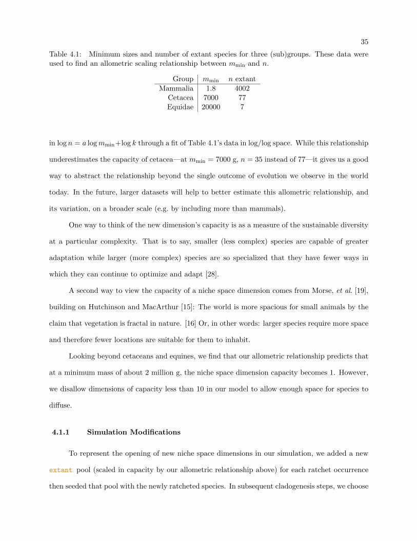
Table 4.1: Minimum sizes and number of extant species for three (sub)groups. These data wereused to find an allometric scaling relationship between mmin and n.
Group mmin n extant
Mammalia 1.8 4002Cetacea 7000 77Equidae 20000 7
in log n = a logmmin+log k through a fit of Table 4.1’s data in log/log space. While this relationship
underestimates the capacity of cetacea—at mmin = 7000 g, n = 35 instead of 77—it gives us a good
way to abstract the relationship beyond the single outcome of evolution we observe in the world
today. In the future, larger datasets will help to better estimate this allometric relationship, and
its variation, on a broader scale (e.g. by including more than mammals).
One way to think of the new dimension’s capacity is as a measure of the sustainable diversity
at a particular complexity. That is to say, smaller (less complex) species are capable of greater
adaptation while larger (more complex) species are so specialized that they have fewer ways in
which they can continue to optimize and adapt [28].
A second way to view the capacity of a niche space dimension comes from Morse, et al. [19],
building on Hutchinson and MacArthur [15]: The world is more spacious for small animals by the
claim that vegetation is fractal in nature. [16] Or, in other words: larger species require more space
and therefore fewer locations are suitable for them to inhabit.
Looking beyond cetaceans and equines, we find that our allometric relationship predicts that
at a minimum mass of about 2 million g, the niche space dimension capacity becomes 1. However,
we disallow dimensions of capacity less than 10 in our model to allow enough space for species to
diffuse.
4.1.1 Simulation Modifications
To represent the opening of new niche space dimensions in our simulation, we added a new
extant pool (scaled in capacity by our allometric relationship above) for each ratchet occurrence
then seeded that pool with the newly ratcheted species. In subsequent cladogenesis steps, we choose
36
ancestors from each pool independently to prevent competition by random choice. We cannot,
however, choose from every pool at every step without consequences for the smaller dimensions.
Nichespace dimensions with smaller capacities need to be scaled appropriately in terms of
model time. In section 2.2 we determined the number of model steps to simulate (tmax) based on
the “real” time we would like the model to run (τ = 250 My), the mean species lifetime (ν = 1.6
My), and the number of species expected to be alive at any given time (n): tmax = τ νn. Thus,
ratcheted (nniche < n0) dimensions require fewer model steps to cover the same amount of “real”
time. To account for this, we only choose to speciate from smaller niche dimensions every n0/nniche
steps, where n0 is the number of species in the seed group at equilibrium and nniche is the smaller
niche space dimension’s capacity.
As a result of altering the speciation rate, our uniform extinction rate (β from Section 2.2.3)
can remain constant throughout the simulation, and in terms of the size of the original niche space
dimension: β = 1/n0.
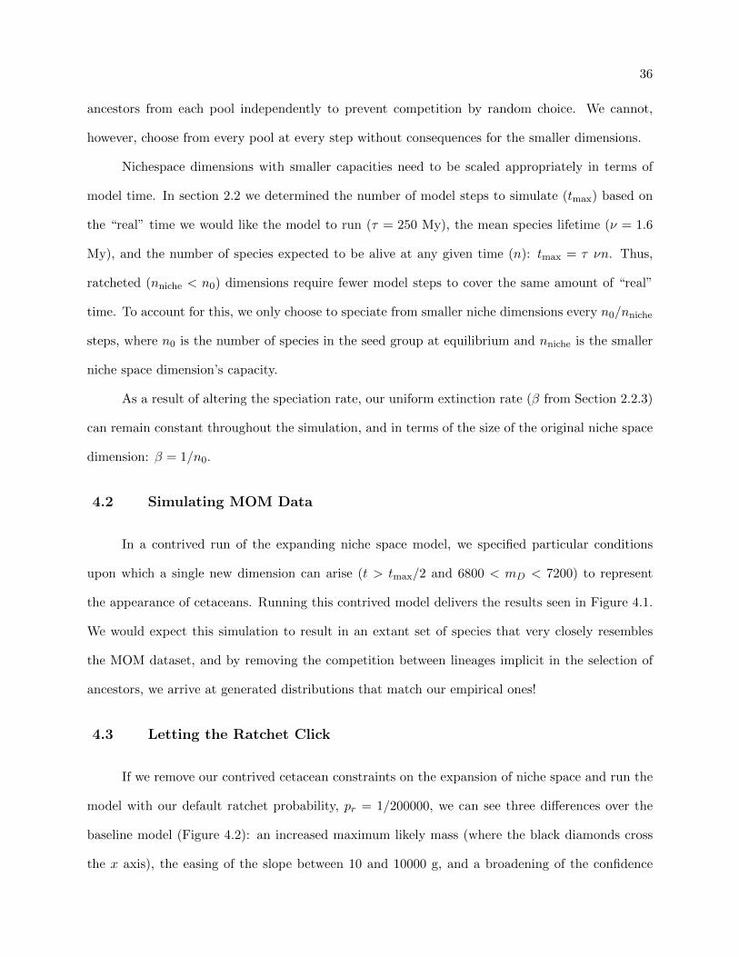
4.2 Simulating MOM Data
In a contrived run of the expanding niche space model, we specified particular conditions
upon which a single new dimension can arise (t > tmax/2 and 6800 < mD < 7200) to represent
the appearance of cetaceans. Running this contrived model delivers the results seen in Figure 4.1.
We would expect this simulation to result in an extant set of species that very closely resembles
the MOM dataset, and by removing the competition between lineages implicit in the selection of
ancestors, we arrive at generated distributions that match our empirical ones!
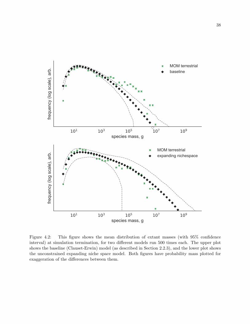
4.3 Letting the Ratchet Click
If we remove our contrived cetacean constraints on the expansion of niche space and run the
model with our default ratchet probability, pr = 1/200000, we can see three differences over the
baseline model (Figure 4.2): an increased maximum likely mass (where the black diamonds cross
the x axis), the easing of the slope between 10 and 10000 g, and a broadening of the confidence

37
101 103 105 107 109
species mass, g
frequ
ency
(log
sca
le),
arb.
a)MOM terrestrialMOM aquaticsim terrestrialsim aquatic
model time
103
105
107
109
1011
larg
est m
ass
seen
, g
b)
model time0
1000
2000
3000
4000
num
ber o
f ext
ant s
peci
es
c)
Figure 4.1: a) shows the distributions of the two niches over the MOM data for reference. b)shows the largest species seen (thicker line), as well as the largest species alive at a given time(thinner line) for both the seed group (green) and the ratcheted group (blue). c) shows the numberof species alive throughout the model for both seed group (green) and ratcheted group (blue).
38
101 103 105 107 109
species mass, g
frequ
ency
(log
sca
le),
arb.
MOM terrestrialbaseline
101 103 105 107 109
species mass, g
frequ
ency
(log
sca
le),
arb.
MOM terrestrialexpanding nichespace
Figure 4.2: This figure shows the mean distribution of extant masses (with 95% confidenceinterval) at simulation termination, for two different models run 500 times each. The upper plotshows the baseline (Clauset-Erwin) model (as described in Section 2.2.3), and the lower plot showsthe unconstrained expanding niche space model. Both figures have probability mass plotted forexaggeration of the differences between them.

39
interval (black dashed line).
All of the differences between the plots in Figure 4.2 are anticipated results of evolving
multiple mass floors: the increase in maximum likely mass was shown by Clauset [7]; the gentler
slope between 10 and 10000 g is explained by the presence of multiple minimum sizes both providing
pressures towards an increase in mass, and preventing smaller masses from appearing; and the
broadening of the confidence interval represents the effects of having different dimensions, each
with unique minimum sizes and capacities, in every run of the model.
From these plots we can also estimate the maximum expected mass of a species. For the
Clauset-Erwin model, this maximum occurs around 107 g—the estimated mass of the extinct Im-
perial Mammoth. For Clauset in [7], the maximum for cetaceans was found to be nearly 7 ∗ 108
g, almost four times the size of a blue whale. In our expanding niche space model, this estimate
(by the edge of the 95% confidence interval) extends out to nearly 1010 g, which is mind-bogglingly
massive.
4.4 Conclusions
In this chapter, we succeeded in simulating the behavior observed in the evolution of cetaceans
from mammals through the removal of implicit competition between groups. This had the effect
of removing genetic drift from our model, allowing the random mutations—ratcheted minimum
masses—to persist.
Chapter 5
Conclusions
At the end of [17], Loreto et al. conclude that an important aspect of any novelty-generating
statistical model is the ability to enlarge the space of possibilities.1 In our model of species
complexity, we generate novelties through random mutation in the absence of genetic drift.
Looking back on our broad questions from Chapter 1, we can now say that (under the as-
sumptions upon which we built this model) increasing complexity occurs as a result of random
mutations and is preserved when a complex collection of those mutations (an evolutionary innova-
tion) allows access to a new dimension of niche space—just as mammals’ endothermy allows them
to survive in more variable environments, or how the emergence of eyes gave organisms an inherent
advantage. Conversely, if an innovation does not promote the lineage to an uncontested dimension,
then one of two things can happen: the innovating lineage may push its ancestors to extinction, or
it may go extinct itself.
So now we can refine our idea of a ratchet in evolution. A ratchet is not simply any irreversible
innovation, but rather one that provides enough of an advantage to elevate the lineage into an
uncontested space.
1 Loreto et al.’s model is based on Polya’s urn—a rich-get-richer statistical model of randomly selecting colored ballsfrom an urn and replacing them along with additional balls depending on what was chosen—which has similar (andmore general) mechanics to our radiation promotion model (Section 3.3.2), if our model did not include extinction.

41
5.1 Future Work
This work is rife with opportunities for continuation, from concrete research tasks to appli-
cations in other fields. Here we present some ideas of how we would choose to continue this line of
research.
5.1.1 Concrete Continuations
Considering the growing popularity and interest in minimum sizes, it would be of value to
the evolutionary biology facet of this study to tabulate more data for the allometric relationship
discussed in Section 4.1, to further support the relationship itself, and to provide an estimate of
the variability in niche space dimension capacity.
Another continuation of this research could be found in applying it to other, non mammal,
Classes. If this model is generalizable to wildly different varieties of organisms (such as insects,
reptiles, or amoeba), it would have major implications in our understanding of macroevolution. A
barrier to completing such research would be the massive amount of data—concerning both extant
and extinct species—required to fit the model with non-mammal parameters.
5.1.2 Other Facets of Ratchets
Here we have shown how the ratcheting of complexity influences body mass in biological
species, but what other evolving entities exhibit ratchets? There are a number of ways this research
on complexity could be broadened—all we need is data.
One area we could explore would be the ecosystem of software and technology. Ratchets
in this domain could include such innovations as the wheel or the Internet—each opening up an
entirely new dimension along which optimization can occur. For a study of technology, patent
records, Github repository data, and other data sources could be compiled for model parameter
estimation.
Another area of interest would be the social ecosystem. Social communities or cities are

42
built very in a similar fashion to complex organisms, with differentiation of expertise coordinating
to grow to sizes unachievable without innovations such as agriculture or language. Businesses and
companies also have many qualities that could be used to measure complexity (number of employees
or reported revenue, for example) and can even be grouped by field of expertise (such as financial,
service, or engineering) for comparison.
Regardless of the complex system being studied, the process of adapting our statistical model
would be similar. After deciding on a metric that correlates with complexity, we can compile
a dataset, examine the distribution of complexity measures, then work to tune parameters of
the model to fit the distribution. What could come out of such a study would be technological
or social corollaries to biologically observed phenomena—i.e. Cope’s Rule and mass-dependent
extinction—resulting in quantifiable interdisciplinary comparisons of evolution across all aspects of
our complicated existence.
Bibliography
[1] Boye K. Ahlborn. Thermodynamic Limits of Body Dimension of Warm Blooded Animals.Journal of Non-Equilibrium Thermodynamics, 25(1):87–102, 2000.
[2] Boye K. Ahlborn and Robert W. Blake. Lower size limit of aquatic mammals. AmericanJournal of Physics, 67(10):920–922, September 1999.
[3] John Alroy. Cope’s Rule and the Dynamics of Body Mass Evolution in North American FossilMammals. Science, 280(5364):731–734, May 1998.
[4] Samuel Arbesman. Overcomplicated: Technology at the Limits of Comprehension. Current,New York, New York, July 2016.
[5] James H. Brown. Macroecology. 1995.
[6] Marcel Cardillo, Georgina M. Mace, Kate E. Jones, Jon Bielby, Olaf R. P. Bininda-Emonds,Wes Sechrest, C. David L. Orme, and Andy Purvis. Multiple Causes of High Extinction Riskin Large Mammal Species. Science, 309(5738):1239–1241, August 2005.
[7] Aaron Clauset. How Large Should Whales Be? PLOS ONE, 8(1):e53967, January 2013.
[8] Aaron Clauset and Douglas H. Erwin. The Evolution and Distribution of Species Body Size.Science, 321(5887):399–401, July 2008.
[9] E. D. Cope. The primary factors of organic evolution. The Open Court Publishing Company,Chicago, London, 1896.
[10] Kenneth W. Desmond and Eric R. Weeks. Influence of particle size distribution on randomclose packing of spheres. Physical Review E, 90(2):022204, August 2014.
[11] Jerry F. Downhower and Lawrence S. Blumer. Calculating just how small a whale can be.Nature, 335(6192):675–675, October 1988.
[12] Douglas H. Erwin and Eric H. Davidson. Response to Comment on ”Gene Regulatory Networksand the Evolution of Animal Body Plans”. Science, 313(5788):761–761, August 2006.
[13] Leonore Fleming and Daniel W. McShea. Drosophila mutants suggest a strong drive towardcomplexity in evolution. Evolution & Development, 15(1):53–62, January 2013.
[14] John H. Gillespie. Population Genetics: A Concise Guide. JHU Press, December 2010. Google-Books-ID: KAcAfiyHpcoC.
44
[15] G. E. Hutchinson and Robert H. MacArthur. A Theoretical Ecological Model of Size Distri-butions Among Species of Animals. The American Naturalist, 93(869):117–125, March 1959.
[16] Jan Kozowski and Adam. T. Gawelczyk. Why Are Species’ Body Size Distributions UsuallySkewed to the Right? Functional Ecology, 16(4):419–432, 2002.
[17] Vittorio Loreto, Vito D. P. Servedio, Steven H. Strogatz, and Francesca Tria. Dynamics onexpanding spaces: modeling the emergence of novelties. arXiv:1701.00994 [physics], pages59–83, 2016. arXiv: 1701.00994.
[18] Donald Ludwig. Uncertainty and the Assessment of Extinction Probabilities. EcologicalApplications, 6(4):1067–1076, November 1996.
[19] D. R. Morse, J. H. Lawton, M. M. Dodson, and M. H. Williamson. Fractal dimension ofvegetation and the distribution of arthropod body lengths. Nature, 314(6013):731–733, April1985.
[20] Oliver P. Pearson. Metabolism of Small Mammals, With Remarks on the Lower Limit ofMammalian Size. Science, 108(2793):44–44, July 1948.
[21] David M. Raup. Probabilistic Models in Evolutionary Paleobiology: A random walk throughthe fossil record produces some surprising results. American Scientist, 65(1):50–57, 1977.
[22] Lauren Shoemaker and Aaron Clauset. Body mass evolution and diversification within horses(family Equidae). Ecology Letters, 17(2):211–220, February 2014.
[23] Lauren Shoemaker and Aaron Clauset. Universal Processes Govern Body Mass Evolution inMarine and Terrestrial Environments. unpublished, 2017.
[24] Felisa A. Smith, Alison G. Boyer, James H. Brown, Daniel P. Costa, Tamar Dayan, S. K. Mor-gan Ernest, Alistair R. Evans, Mikael Fortelius, John L. Gittleman, Marcus J. Hamilton,Larisa E. Harding, Kari Lintulaakso, S. Kathleen Lyons, Christy McCain, Jordan G. Okie,Juha J. Saarinen, Richard M. Sibly, Patrick R. Stephens, Jessica Theodor, and Mark D. Uhen.The Evolution of Maximum Body Size of Terrestrial Mammals. Science, 330(6008):1216–1219,November 2010.
[25] FelisaA. Smith, JamesH. Brown, JohnP. Haskell, S.Kathleen Lyons, John Alroy, EricL. Char-nov, Tamar Dayan, BrianJ. Enquist, S.K. Morgan Ernest, ElizabethA. Hadly, KateE. Jones,DawnM. Kaufman, PabloA. Marquet, BrianA. Maurer, KarlJ. Niklas, WarrenP. Porter, BruceTiffney, MichaelR. Willig, and Associate Editor: Jonathan B. Losos. Similarity of Mamma-lian Body Size across the Taxonomic Hierarchy and across Space and Time. The AmericanNaturalist, 163(5):672–691, 2004.
[26] Wisconsin Human Society. Were over the moon: Wisconsin Humane Society adopts out itssmallest dog ever, January 2017.
[27] S. M. Stanley. A theory of evolution above the species level. Proceedings of the NationalAcademy of Sciences, 72(2):646–650, February 1975.
[28] Steven M. Stanley. An Explanation for Cope’s Rule. Evolution, 27(1):1–26, 1973.

45
[29] Leigh Van Valen. Body Size and Numbers of Plants and Animals. Evolution, 27(1):27–35,1973.
[30] Geoffrey B. West, William H. Woodruff, and James H. Brown. Allometric scaling of metabolicrate from molecules and mitochondria to cells and mammals. Proceedings of the NationalAcademy of Sciences, 99(suppl 1):2473–2478, February 2002.
[31] Richard J. Williams, Ananthi Anandanadesan, and Drew Purves. The Probabilistic NicheModel Reveals the Niche Structure and Role of Body Size in a Complex Food Web. PLOSONE, 5(8):e12092, August 2010.

Appendix A
Model Subtleties
A.1 Seed Mass
You can seed the baseline model, as described in 2.2.3 with any mass and get the same final
distribution. Figure A.1 shows this graphically.
101 103 105 107 109
species mass, g
dens
ity (l
og s
cale
), ar
b. MOM terrestrialm_0 = 2
101 103 105 107 109
species mass, g
dens
ity (l
og s
cale
), ar
b. MOM terrestrialm_0 = 7000
101 103 105 107 109
species mass, g
dens
ity (l
og s
cale
), ar
b. MOM terrestrialm_0 = 20000
101 103 105 107 109
species mass, g
dens
ity (l
og s
cale
), ar
b. MOM terrestrialm_0 = 1000000
Figure A.1: Four plots showing the baseline model (see Section 2.2.3) output for four differentinitially masses: 2, 7000, 20000, and 1000000 g. Each initial mass was run through the model 100times; plotted is the mean (black diamonds) and 95% confidence interval (dashed black lines) ofthose runs over the MOM terrestrial data (green Xs).

47
A.2 Effects of ratchet probability on simulation results
Increasing the ratchet probability of the naıve model causes the distribution to spread out
even further, increasing the mode and the maximum. Figure A.2 depicts this effect through four
different ratchet probabilities. The model was run 100 times at each probability; shown are the
means and the 95% confidence intervals for those 100 runs.
101 103 105 107 109
species mass, g
dens
ity (l
og s
cale
), ar
b.
MOM terrestrialp_r = 0.00005
101 103 105 107 109
species mass, g
dens
ity (l
og s
cale
), ar
b.
MOM terrestrialp_r = 0.0005
101 103 105 107 109
species mass, g
dens
ity (l
og s
cale
), ar
b.
MOM terrestrialp_r = 0.005
101 103 105 107 109
species mass, g
dens
ity (l
og s
cale
), ar
b.
MOM terrestrialp_r = 0.05
Figure A.2: Four plots showing the naıve ratcheting model (see Section 2.2.3) output for fourdifferent ratchet probabilities: 1/200000, 1/20000, 1/2000, and 1/200. Each plot represents the themean (black diamonds) and 95% confidence interval (dashed black lines) for 100 runs of the model,shown over the MOM terrestrial data (green Xs) for reference.
A.3 Histogram Normalization
To keep the figures in the document consistent, we used probability density histograms for
most plots. To illustrate the visual differences between two ways of normalizing histograms, we
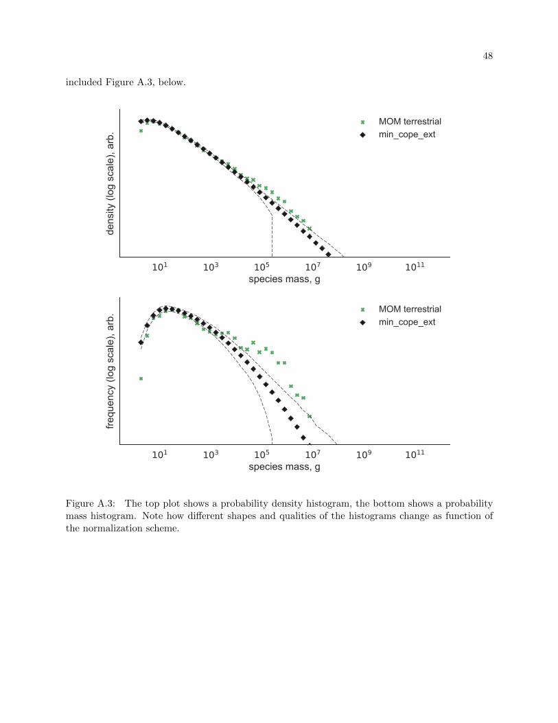
48
included Figure A.3, below.
101 103 105 107 109 1011
species mass, g
dens
ity (l
og s
cale
), ar
b.MOM terrestrialmin_cope_ext
101 103 105 107 109 1011
species mass, g
frequ
ency
(log
sca
le),
arb.
MOM terrestrialmin_cope_ext
Figure A.3: The top plot shows a probability density histogram, the bottom shows a probabilitymass histogram. Note how different shapes and qualities of the histograms change as function ofthe normalization scheme.
Appendix B
Extinction-Centric Model
There is another way that we conceived of to remove the inherent competition in species
choice, which contained an opportunity to relax the model of cladogenesis we used to be more
general. By refactoring the model (from speciation at every iteration) to be based on extinction
events, we programmed an “extinction-centric” version of the model.
The move from an iteration- to event-based method of modeling brings along some challenges
for performing efficiently. Instead of choosing directly from a collection of species we know to be
extant at the time of cladogenesis, we will be waiting until a species goes extinct before executing
the speciation step. This means that, to have our simulation terminate in a reasonable time we
need to be able to tell when the next species will be going extinct, and “fast-forward” the model
to that time.
To pre-determine a species’ extinction date efficiently, we used a geometric distribution (the
discrete trial analog to an exponential distribution) to model the number of trials we would have
needed to perform (at pext) to get our first success—where “success” here denotes extinction.
This condenses thousands of random draws into one, making our model more performant. We
implemented the geometric distribution computationally by taking a uniform-at-random draw from
[0, 1]—standard call to most any random function—as the result of draw from the cumulative
distribution function (CDF) of an exponential distribution, and calculated which input value to
the CDF would have given us our randomly drawn outcome. Mathematically, we solve for x in
random() = 1 − exp−λx, where λ = 1/pext—resulting in x = log random()/ log(1 − pext). If we
50
are working with discrete time steps, we then take the floor of x to map it from the continuous
exponential distribution to the discrete event geometric distribution; otherwise we can scale the
resultant x by a factor of millions of years to get a “real time” extinction pre-determination. (Note
that we incorporated the discrete-time method of extinction determination into the Clauset-Erwin
model as well; see Section 2.2.)
Now that we know when a species will go extinct as soon as it spawns, we need to choose
appropriate data structures to keep track of what events (extinction or speciation) are coming up
next. We opted to use a binary heap to keep our extinction events ordered (O(log n) for insertion
and for popping largest, due to contents being sorted by key); a hash map for quick, random-
access bookkeeping of which species are extant (expected and amortized O(1) insert, expected
O(1) remove); and a vector for keeping record of every species seen (amortized O(1) insertion at
end). This collection of data structures allows for very rapid and simple determination of the next
upcoming event.
Right away we run into an issue with the model that we did not have to account for previously:
reaching our equilibrium species count, n. In our speciation-centric model we iterate with every
speciation event such that the extinction pressure stays constant, causing the species count to
reach n and enter equilibrium after t = n steps. However, in our extinction-centricmodel we link
speciation events to extinction events and iterate on extinction, meaning that we will not have
radiation in the model during the first n steps. As such, n is no longer a stable attractor for
species count; rather species count will perform a random walk. To address this, we have to make
speciation events more common (pspec > 0.5) while t < n, and then let the probability of speciation
to dwindle to the equilibrium probability of ps = 0.5 once t > n.
B.1 Relaxing Cladogenesis
To relax our model of cladogenesis, which we naıvely chose to result in the emergence of
two new species and extinction of the progenitor, we can assume that speciation events—like
extinction events—are distributed throughout time like a Poisson process. As such, we can give a
51
“speciation rate” as input, and draw speciation event timing from an exponential distribution as
well, disassociating speciation from extinction and adding a new type of event to our model.
Making both speciation and extinction events independent in time relaxes our model of
cladogenesis by allowing outcomes such as anagenesis (one new species upon extinction, as a result
of accumulated changes) and the continuation of the progenitor species after speciation. The
drawback here—and ultimately the reason this line of inquiry was closed—is the addition of a
difficult-to-estimate parameter to the model: speciation rate.
B.2 Outcomes
It was abandoned due to time constraints and due to the increased parameter space (by
introducing a speciation rate) that made fitting the model extremely difficult. In the end, the
extinction-centricmodel is still beholden to competition through selection due to the limited capacity
of the extant pool.