1
Quantized Precoding for Massive MU-MIMOSven Jacobsson, Giuseppe Durisi, Mikael Coldrey, Tom Goldstein, and Christoph Studer
Abstract
Massive multiuser (MU) multiple-input multiple-output (MIMO) is foreseen to be one of the key
technologies in fifth-generation wireless communication systems. In this paper, we investigate the problem
of downlink precoding for a narrowband massive MU-MIMO system with low-resolution digital-to-analog
converters (DACs) at the base station (BS). We analyze the performance of linear precoders, such as
maximal-ratio transmission and zero-forcing, subject to coarse quantization. Using Bussgang’s theorem,
we derive a closed-form approximation of the achievable rate of the coarsely quantized system. Our
results reveal that the infinite-resolution performance can be approached with DACs using only 3 to 4 bits
of resolution, depending on the number of BS antennas and the number of user equipments (UEs). For the
case of 1-bit DACs, we also propose novel nonlinear precoding algorithms that significantly outperform
linear precoders at the cost of an increased computational complexity. Specifically, we show that nonlinear
precoding incurs only a 3 dB penalty compared to the infinite-resolution case for an uncoded bit error
rate of 10−3 in a system with 128 BS antennas that uses 1-bit DACs and serves 16 single-antenna UEs;
in contrast, the penalty is about 8 dB for linear precoders.
Index Terms
Massive multi-user multiple-input multiple-output, digital-to-analog converter, Bussgang’s theorem,
minimum mean-square error precoding, convex optimization, semidefinite relaxation, Douglas-Rachford
splitting, sphere precoding.
S. Jacobsson is with Ericsson Research and Chalmers University of Technology, Gothenburg, Sweden (e-mail: [email protected]).
G. Durisi is with Chalmers University of Technology, Gothenburg, Sweden (e-mail: [email protected]).
M. Coldrey is with Ericsson Research, Gothenburg, Sweden (e-mail: [email protected])
T. Goldstein is with the Department of Computer Science, University of Maryland, College Park, MD (e-mail: [email protected]).
C. Studer is with the School of Electrical and Computer Engineering, Cornell University, Ithaca, NY (e-mail: [email protected]).
The work of S. Jacobsson and G. Durisi was supported by the Swedish Foundation for Strategic Research under grantsSM13-0028 and ID14-0022, and by the Swedish Governmental Agency for Innovation Systems (VINNOVA) within the VINNExcellence center Chase.
The work of T. Goldstein was supported in part by the US National Science Foundation (NSF) under grant CCF-1535902 andby the US Office of Naval Research under grant N00014-15-1-2676.
The work of C. Studer was supported in part by Xilinx Inc. and by the US NSF under grants ECCS-1408006 and CCF-1535897.
The system simulator for quantized precoding will be made available on GitHub upon (possible) acceptance of the paper.

2
I. INTRODUCTION
Massive multiuser (MU) multiple-input multiple-output (MIMO) wireless systems, where the base
station (BS) is equipped with several hundreds of antenna elements, promises significant improvements in
spectral efficiency, energy efficiency, reliability, and coverage compared to traditional cellular systems [1]–
[3]. Increasing the number of radio frequency (RF) chains at the BS could, however, lead to significant
increases in hardware complexity, system costs, and circuit power consumption. Therefore, practical
massive MU-MIMO systems may require low-cost and power-efficient hardware components at the BS.
In this paper, we consider the downlink of massive MU-MIMO system, where the BS is equipped
with low-resolution digital-to-analog converters (DACs) and transmits data to multiple, independent user
equipments (UEs) in the same time-frequency resource.
For the quantization-free case (infinite-resolution DACs), the capacity region of the MU downlink
Gaussian channel has been characterized in [4]–[7]. When channel state information (CSI) is known
noncausally at the BS, dirty-paper coding (DPC) [8] is known to achieve the sum-rate capacity [6]. Several
precoding algorithms to approach the DPC performance have been proposed (see, e.g., [9]–[12]). Most of
these precoding methods are, however, computationally demanding, and their complexity scales unfavorably
with the number of BS antennas, preventing their use for massive MU-MIMO. Linear precoding, on the
other hand, is an attractive low-complexity approach to massive MU-MIMO downlink precoding, which
offers competitive performance to DPC for large antenna arrays [13], [14].
These results assume that the RF circuitry connected to each antenna port at the BS is ideal. The impact
of RF hardware impairments at the transmit side has been investigated in, e.g., [15]–[18]. Some of these
results indicate that massive MU-MIMO exhibits a certain degree of resilience against RF impairments.
The crude aggregate models used for characterizing such hardware impairments, however, are unable to
accurately capture the distortion caused by low-resolution DACs.
A. What are the Benefits of Quantized Massive MU-MIMO?
One of the dominant sources of power consumption in massive MU-MIMO systems are the data
converters at the BS. In the downlink, the transmit baseband signal at each RF chain is generated by a
pair of DACs. The power consumption of these DACs increases exponentially with the resolution (in
bits) and linearly with the bandwidth [19], [20]. In traditional multi-antenna systems, each RF port is
connected to a pair of high-resolution DACs (e.g., 10-bit or more). For massive MU-MIMO systems with
hundred or even thousands of antenna elements, this would lead to prohibitively high power consumption
due to the large number of required DACs. Hence, the DAC resolution must be limited to keep the power
budget within tolerable levels. In addition, the use of low-resolution DACs enables one to reduce the

3
linearity and noise requirements of the surrounding RF circuitry; this has the potential to further reduce
the power consumption and costs of the RF circuits at the BS. Furthermore, an often overlooked issue in
massive MU-MIMO is the vast amount of data that must be transmitted from the fronthaul link to the
baseband-processing unit. To make matters worse, in many deployment scenarios, these two units are
separated by a large distance. Hence, lowering the DAC resolution is a potential solution to mitigate the
data-rate bottleneck of the fronthaul link.
B. Relevant Prior Art
1) Quantized Receivers: Several recent contributions have studied the use of low-resolution analog-to-
digital converters (ADCs) for the massive MU-MIMO uplink. In particular, there has been a significant
interest in the 1-bit ADC case. For frequency-flat channels, the performance of 1-bit ADCs followed by
linear detectors was analyzed in, e.g., [21]–[23], where it was shown that large achievable sum rates are
supported. Similar conclusions were made in [24] for the frequency-selective case. Coarse quantization
and nonlinear detection algorithms for frequency-selective channels were studied in [25], where it was
found that 4 to 6 bits are sufficient to close the gap to the infinite-resolution case.
2) Low-PAR and Constant-Envelope Precoding: Hardware-aware precoding has previously been
considered for massive MU-MIMO, with the goal of reducing the linearity requirements at the BS.
In [26], the problem of joint MU precoding and peak-to-average power ratio (PAR) reduction was achieved
by solving a convex optimization problem. Constant-envelope precoding was studied in [27], [28], which
minimizes the PAR by transmitting constant-modulus signals only.
3) Quantized Precoding: In contrast to the uplink case, there has only been a small number of
contributions that consider the massive MU-MIMO downlink with low-resolution DACs at the BS. In [29],
the authors designed a linear-quantized precoder based on the minimum mean-square error (MMSE)
criterion, taking into account the distortion caused by the DACs. For DACs with 4 to 6 bits resolution,
the precoder proposed in [29] is shown to outperform conventional linear-quantized precoders for small-
to-moderate-sized MIMO systems at high signal-to-noise ratio (SNR). Massive MU-MIMO systems with
1-bit DACs are investigated in [30], where it is shown that maximal ratio transmission (MRT) precoding
results in manageable distortion levels. Still for the case of 1-bit DACs, zero-forcing (ZF) precoding for a
Rayleigh-fading channel is considered in [31]. Interestingly, the authors show that the received signal can
be made proportional to the transmitted signal when the number of BS antennas tend to infinity. This
shows that the severe per-antenna distortion caused by the 1-bit DACs averages out over the antenna array.
A linear precoder where the 1-bit quantized outcomes are rescaled in the analog domain was presented
4
in [32]. There, the authors use the gradient projection algorithm to find a precoder that yields improved
performance over the one reported in [29].
C. Contributions
We consider quantized precoding for the massive MU-MIMO downlink in frequency-flat channels. In
contrast to [30]–[32], we do not restrict ourselves to 1-bit DACs and linear precoding. Specifically, we
consider both linear-quantized precoders, where a linear precoder is followed by a finite-resolution DAC,
and nonlinear precoders, where the data vector together with the CSI is used to directly generate the
DAC outputs. Our contributions can be summarized as follows.
• We formulate the MMSE-optimal linear-quantized precoding problem and present low complexity,
suboptimal linear-quantized precoders that yield approximate solutions to this problem. We use
Bussgang’s theorem to develop simple closed-form approximations for the rate achievable with
linear-quantized precoding and low-resolution DACs. Through numerical simulations, we validate the
accuracy of these approximations, and we show that only a small number of quantization bits are
sufficient to close the performance gap to the infinite-resolution case. For the special case of 1-bit
DACs, we develop a sharp lower bound on the achievable rate with linear precoding.
• For the 1-bit case, we develop a variety of low-complexity nonlinear precoders that achieve near-
optimal performance. We show that the MMSE-optimal downlink precoding problem can be relaxed to
a convex problem that can be solved in a computationally-efficient manner. We propose computationally
efficient algorithms based on semidefinite relaxation, squared-`∞ norm relaxation, and sphere decoding,
and we discuss advantages and limitations of each of these methods. Through numerical simulations,
we demonstrate the superiority of nonlinear precoding over linear-quantized precoding.
• We investigate the sensitivity of the proposed precoders to channel-estimation errors and demonstrate
that the proposed precoders are robust to imperfect CSI at the BS.
Our results reveal that massive MU-MIMO enables the use of low-resolution DACs at the BS without
a significant performance loss in terms of error-rate performance and information-theoretic rates.
D. Notation
Lowercase and uppercase boldface letters designate column vectors and matrices, respectively. For a
matrix A, we denote its complex conjugate, transpose, and Hermitian transpose by A∗, AT , and AH ,
respectively. The entry on the kth row and on the `th column is [A]k,`. For a vector a, the kth entry
is [a]k. We use A 0 to indicate that the matrix A is positive semidefinite. The trace and the main
diagonal of A are tr(A) and diag(A), respectively. The M ×M identity and the all-zeros matrix are

5
det.
freq
uen
cy-f
lat
wir
ele
ss c
han
nel
pre
coder
. .
.
DAC
. .
.
RFmap.
RF
RF
RF
RF
RF
DAC
DACDAC
DACDAC
. .
.
. .
.
. .
.
map.
map.
det.
det.
Fig. 1. Overview of the proposed quantized massive MU-MIMO downlink system. Left: B antenna massive MU-MIMO BS thatperforms quantized precoding to enable the use of low-resolution DACs; Right: U single-antenna UEs.
denoted by IM and 0M×N , respectively. The real and imaginary parts of a complex vector a are <aand =a, respectively. We use ‖a‖2 and ‖a‖∞ to denote the `2-norm and the `∞-norm of a, respectively.
We use sgn(·) to denote the signum function, which is applied entry-wise to a vector and defined
as sgn(a) = +1 for a ≥ 0 and sgn(a) = −1 for a < 0. We further use 1A(a) to denote the indicator
function, which is defined as 1A(a) = 1 for a ∈ A and 1A(a) = 0 for a /∈ A. The multivariate complex-
valued circularly-symmetric Gaussian probability density function (PDF) with covariance matrix K is
denoted by CN (0,K). We use f(·) to denote PDFs and Ex[·] to denote expectation in the random
vector x. The mutual information between two random vectors x and y is written as I(x;y).
E. Paper Outline
The rest of the paper is organized as follows. Section II introduces the system model and formulates
the MMSE-optimal quantized precoding problem. Section III investigates linear-quantized precoders
for massive MU-MIMO systems. Section IV deals with nonlinear precoding algorithms for the case of
1-bit DACs. Section V provides numerical simulation results and analyzes the robustness of the developed
algorithms to channel-estimation errors. We conclude the paper in Section VI.
II. SYSTEM MODEL AND QUANTIZED PRECODING
A. System Model
We consider the downlink of a single-cell massive MU-MIMO system as illustrated in Fig. 1. The
system consists of a BS with B antennas that serves U single-antenna UEs simultaneously and in the
same time-frequency resource. The input-output relation of the downlink channel is modeled as
y = Hx + n. (1)

6
Here, the vector y = [y1, . . . , yU ]T contains the received signals at all users, where yu ∈ C is the signal
received at the uth UE. The matrix H ∈ CU×B models the downlink channel, and it is assumed to be
perfectly known to the BS.1 We shall also assume that the entries of H are independent circularly-symmetric
complex Gaussian random variables with unit variance, i.e., hu,b = [H]u,b ∼ CN (0, 1), for u = 1, . . . , U ,
and b = 1, . . . , B. The vector n ∈ CU in (1) models additive noise. We assume the noise to be i.i.d.
circularly-symmetric complex Gaussian with variance N0 per complex entry, i.e., nu ∼ CN (0, N0),
for u = 1, . . . , U . We shall also assume that the noise level is known perfectly at the BS.2
The precoded vector is denoted by x ∈ XB , where X represents the transmit alphabet; this set coincides
with the set C of complex numbers in the case of infinite-resolution DACs. In real-world BS architectures
with finite-resolution DACs, the set X is, however, a finite-cardinality alphabet. Specifically, we denote the
set of possible real-valued DAC outputs (quantization labels) as L = `0, . . . , `L−1. We refer to L = |L|and Q = log2 L as the number of quantization levels and the number of quantization bits per real
dimension, respectively. For each BS antenna, we assume the same quantization alphabet for the real
and the imaginary parts. Hence, the set of complex-valued DAC outputs at each antenna is X = L × L.
Under these assumptions, the bth entry of the precoded vector x is xb = `R + j`I where `R, `I ∈ L.
B. Precoding
The goal of precoding is to transmit constellation points su ∈ O for u = 1, . . . , U to each UE u, where Ois the set of constellation points (e.g., QPSK). The BS uses the available CSI, namely the noncausal
knowledge of the realization of the channel matrix H, to precode the symbol vector s = [s1, . . . , sU ]T
into a B-dimensional precoded vector x = P(s,H). Here, the function P(·, ·) : OU × CU×B → XB
represents the precoder. The precoded vector x must satisfy the average power constraint
Es
[‖x‖22
]≤ P. (2)
We define ρ = P/N0 as the SNR.
Coherent transmission of data using multiple BS antennas leads to a array gain, which depends on the
realization of the fading channel. We shall assume that the uth UE is able to rescale the received signal yu
by a factor βu ∈ R to compute an estimate su ∈ C of the transmitted symbol su ∈ O as follows:
su = βuyu. (3)
1In Section V-B, we will relax this assumption by investigating the impact of imperfect CSI to the robustness of the proposedquantized precoding algorithms.
2Knowledge of N0 at the BS can be obtained by explicit feedback from the UEs to the BS.

7
×s
P(H)
Q(·) x
(a) Linear-quantized precoders: the precoder uses H todesign a precoding matrix P. The transmit vector is thequantized version of Ps, i.e., x = Q(Ps). Here, Q(·)denotes the quantizers.
P(·, ·)s
Hx
(b) Nonlinear precoders: the precoder uses H to directlycompute the quantized transmit vector x ∈ XB as a nonlinearfunction of s and H, i.e., x = P(s,H).
Fig. 2. Illustration of linear-quantized (a) and nonlinear (b) precoders.
The problem of downlink precoding has been studied extensively in the literature. Broadly speaking,
the goal is to increase the signal power to the intended UEs while simultaneously reducing MU
interference (MUI) [33]. There exist multiple formulations of this optimization problem based on different
performance metrics (sum-rate throughput, worst-case throughput, error probability, etc.). We refer the
interested reader to the tutorial [34] for a comprehensive overview.
Our goal is to design a precoder that minimizes the MSE between the estimated symbol vector s =
[s1, . . . , sU ]T and the transmitted symbol vector s under the power constraint (2). This problem has been
studied extensively for the case of infinite-resolution DACs (see, e.g., [35]–[37]).
If the BS is equipped with finite-resolution DACs, then the UEs will experience additional distortion
compared to the infinite-resolution case, due to finite cardinality of the set XB of possible precoder outputs.
This implies that finding the MMSE-optimal precoder for BS architectures with finite-resolution DACs is
a formidable task. In what follows, we present novel algorithms that efficiently compute approximate
solutions to the quantized precoding problem. More specifically, we investigate two fundamentally distinct
approaches: linear-quantized precoding (in Section III) and nonlinear-quantized precoding for the special
case of 1-bit DACs (in Section IV). As illustrated in Fig. 2, linear-quantized precoders first perform linear
processing (matrix-vector multiplication) followed by quantization; in contrast, nonlinear precoders use
the transmit vector s together with the available CSI in order to directly compute the precoded vector x.
As it will be shown in Section V, nonlinear precoders outperform (often significantly) linear-quantized
precoders in terms of error-rate performance at the cost of higher computational complexity.
III. LINEAR–QUANTIZED PRECODERS
In the infinite-resolution case, linear precoders multiply the U -dimensional symbol vector s with
a precoding matrix P ∈ CB×U so that x = Ps. This approach is particularly attractive for massive

8
MU-MIMO systems due to (i) the relatively low computational complexity and (ii) the fact that even the
simplest linear precoder, namely the MRT precoder, achieves virtually optimal performance in the large-
antenna limit; see, e.g., [1]. Linear-quantized precoders inherit the first of these two advantages. Indeed,
quantizing the precoded vector implies no additional computational complexity. For linear-quantized
precoders, the precoded vector x ∈ XB is given by
x = Q(Ps). (4)
Here, Q(·) : CB → XB denotes the quantizer-mapping function, which is a nonlinear function that
describes the joint operation of the 2B DACs at the BS.
The remainder of this section is organized as follows. We start by formulating the MMSE quantized
precoding problem for linear-quantized precoders. We then describe the operation of the DACs and
define the quantizer-mapping function. We then use Bussgang’s theorem [38] to derive a lower bound
on the sum-rate capacity for the case of 1-bit DACs at the BS. Finally, we derive a simple closed-form
approximation of the rate achievable with Gaussian inputs for the more general case of Q-bit DACs.
A. The Linear-Quantized Precoding Problem
By restricting ourselves to linear-quantized precoding (LQP), the MMSE quantized precoding problem
can be formulated as follows:
(LQP)
minimize
P∈CB×U , β∈REs
[‖s− βHQ(Ps)‖22
]+ β2UN0
subject to Es
[‖x‖22
]≤ P and β > 0.
(5)
The resulting precoding matrix PLQP and the associated scalar βLQP are referred to as the optimal solution
to the problem (LQP). Here, we have introduced the parameter β ∈ R to account for the array gain.
In (LQP), we have restricted ourselves to the case in which the precoder results in the same gain β ∈ R
for all UEs. For this case, the per-channel MSE between the transmitted symbols s and the estimated
symbols s = βy can be written as
Es
[‖s− s‖22
]= Es
[‖s− βHx‖22
]+ β2UN0. (6)
By replacing x = Q(Ps), we recognize (6) as the objective function in (5). Note that the array gain the
precoder attempts to achieve may differ from the actual array gain experienced by the uth UE. Therefore,
we let each UE scale the received signal by an individual factor βu, for u = 1, . . . , U (see Fig. 1).
Solving (5) in closed form is a challenging task due to the nonlinear operation of the DACs, captured by
the quantizer-mapping function Q(·). An approximate solution to (5) was presented in [29]. This solution

9
is obtained by approximating the statistics of the distortion caused by the DACs. We shall consider a
different approach. Specifically, we design linear precoders that assume infinite-resolution DACs at the
BS, and then quantize the resulting precoded vector. Such linear-quantized precoders have the advantage
that the precoding matrix P does not depend on the resolution of the DACs. Furthermore, as we shall see
in Section V-A, the difference in error-rate performance between the precoders found using our approach
and the precoder presented in [29] is negligible. We next review a variety of linear precoding algorithms.
1) WF precoding: For the case when the BS is equipped with infinite-resolution DACs, the solution
to (5) is the Wiener filter (WF) precoder [36]:
PWF =1
βWFHH(HHH + UN0IU )−1 (7)
where
βWF =
√1
Ptr((HHH + UN0IU )−1HHH(HHH + UN0IU )−1). (8)
We write the resulting precoded vector as xWF = Q(PWFs
).
2) ZF precoding: With ZF precoding, the BS nulls the multiuser interference by choosing as precoding
matrix the pseudo-inverse of the channel matrix. The ZF precoding matrix is obtained from (7) by
setting the noise variance N0 to zero, which yields PZF = 1βZFH
†, where H† = HH(HHH)−1 is the
pseudo-inverse of the channel matrix H, and βZF =√
1P tr((HHH)−1). The resulting precoded vector
is xZF = Q(PZFs
).
3) MRT precoding: The MRT precoder maximizes the power directed towards each UE, ignoring MUI.
The precoding matrix can be obtained from (7) by letting the noise variance N0 tend to infinity, which yields
PMRT = 1βMRTBH
H and βMRT = 1B
√1P tr(HHH). The resulting precoded vector is xMRT = Q
(PMRTs
).
B. Uniform Quantization of a Complex-Valued Vector
We shall model the DACs as symmetric uniform quantizers with step size ∆. When a signal is quantized,
the average power in the signal is in general not preserved. Therefore, we further assume that the output
of the quantizer is scaled by a constant α ∈ R, to ensure that the transmit power constraint (2) remains
to be satisfied. We start by defining a set of quantization labels L = `0, . . . , `L with entries
`i = α∆
(i− L− 1
2
), i = 0, . . . , L− 1. (9)

10
Furthermore, let T = τ0, . . . , τL, where −∞ = τ0 < τ1 < · · · < τL−1 < τL = ∞ specify the set
of L+ 1 quantization thresholds. For uniform quantizers, the quantization thresholds are given by
τi = ∆
(i− L
2
), i = 1, . . . , L− 1. (10)
The quantizer-mapping function Q(·) can uniquely be described by the set of quantization labels L and
the set of quantization thresholds T . The DACs map z ∈ C with entries zb into the quantized output x
with entries xb in the following way: if <zb ∈ [τk, τk+1) and =zb ∈ [τl, τl+1), then xb = `k + j`l.
The step size ∆ of the quantizers should be chosen to minimize the distortion between the quantized and
nonquantized vector. Unfortunately, the optimal step size ∆ depends on the distribution of the input [39],
which in our case depends on the precoder and on the signaling scheme. We therefore simply set the
labels and thresholds so as they minimize the distortion under the assumption that the per-antenna input
to the quantizers is CN (0, P/B)-distributed. The optimal step size can then be found numerically (see
e.g., [40] for details).
In the extreme case of 1-bit DACs, the quantizer-mapping function reduces to
Q(z) =
√P
2B
(sgn(<z) + j sgn(=z)
). (11)
Here, we have chosen the set of possible complex-valued quantization outcomes per antenna to be X =
√P/(2B) (±1± j), which ensures that the power constraint in (2) is satisfied with equality.
C. Signal Decomposition using Bussgang’s Theorem
Quantizing the precoded signal causes a distortion Q(Ps)−Ps that is correlated with the input of the
quantizer. However, for Gaussian inputs, Bussgang’s theorem [38] allows us to decompose the quantized
signal into linear function of the input to the quantizers and a distortion term that is uncorrelated with
the input to the quantizers [41]. This will allow us to characterize the achievable rates with Gaussian
inputs. We start by stating Bussgang’s theorem [38], [41].
Theorem 1: Consider two zero-mean jointly complex Gaussian random variables x and y. Assume
that x is passed through a nonlinear function g(·) : C → C that acts independently on the real and
imaginary components of x. Then, the covariance between g(x) and y is given by
E[g(x)y∗] =E[g(x)x∗]
E[xx∗]E[xy∗] . (12)
Bussgang’s theorem has recently been used to analyze massive MU-MIMO uplink systems with 1-bit
ADCs (see, e.g., [23], [24]). It was also used in [30] to approximate the resulting distortion levels caused

11
by MRT precoding and 1-bit quantization in the massive MIMO downlink. We shall use Theorem 1 to
characterize the performance of linear precoding subject to quantization with Q-bit uniform DACs. As a
first step, we establish the following result, whose proof is given in Appendix A.
Theorem 2: Let x = Q(Ps) denote the output from a set of uniform quantizers described by the
quantizer-mapping function Q : CB → XB . Assume that P ∈ CB×U and s ∼ CN (0, IU ). Then, the
quantized vector x can be decomposed as
x = GPs + d, (13)
where the distortion d and the signal s are uncorrelated. Furthermore, G ∈ RB×B is the following
diagonal matrix:
G =α∆√π
diag(PPH
)−1/2L−1∑i=1
exp
(−∆2
(i− L
2
)2
diag(PPH
)−1
). (14)
Here, L and ∆ denote the number of levels and the step size of the DACs, respectively.
The following corollary is a well-known result for the case of 1-bit quantization (see, e.g., [23], [24]).
The proof follows from setting in (14) L = 2 and α∆ =√
2P/B to satisfy the power constraint in (2).
Corollary 3: For the case of 1-bit DACs, the matrix G in (14) reduces to
G =
√2P
πBdiag
(PPH
)−1/2. (15)
Let now hTu denote the uth row of the channel matrix H and pu the uth column of the precoding
matrix P. Using (13), we can express the received signal yu at UE u as follows:
yu = hTu (GPs + n) = hTuGpusu +∑
v 6=u hTuGpvsv + hTud︸ ︷︷ ︸
=eu
+hTun︸︷︷︸=nu
= hTuGpusu + eu + nu. (16)
Here, the error term eu captures both the MUI and the distortion caused by the finite-resolution DACs.
Note that eu and su are uncorrelated. Indeed,
Es[eus∗u] =
∑v 6=u h
TuGpv Es[svs
∗u] + hTu Es[ds
∗u] = 0. (17)
We shall next use the decomposition in (16) to analyze the performance of linear-quantized precoders.

12
D. Achievable Rate Lower Bound for 1-bit DACs
We assume that each UE is able to scale its received signal yu by βu = (hTuGpu)−1 to obtain the
following estimate:
su = βuyu = su + βu(eu + nu). (18)
Learning βu requires each UE to be able to estimate accurately its channel gain. This is a reasonable
assumption provided that the channel coherence interval is sufficiently long [42].
The nonlinear operation of the DACs prevents one to characterize the probability distribution of the
error term eu in closed form, which makes it difficult to compute the achievable rates. One can, however,
lower-bound the achievable rate using the so called "auxiliary-channel lower bound" [43, p. 3503], which
gives the rates achievable with a mismatched decoder (see [44, ch. 1] for a recent review on the subject).
As auxiliary channel, we take the one with output
su = su + βu(eu + nu), (19)
where eu ∼ CN(0,Es
[|eu|2
])has the same variance as the actual error term eu but is Gaussian distributed.
This auxiliary channel is relevant for the case of nearest-neighbor decoding (also known as minimum
distance decoding). Then, by standard manipulations of the mutual information, we can bound the
achievable rate Ru for UE u = 1, 2, . . . , U as follows:
Ru = EH[ I(su; su |H)] (20)
= Esu,su,H[log2
(fsu|su,H(su|su,H)
fsu |H(su |H)
)](21)
≥ Esu,su,H[log2
(fsu|su,H(su|su,H)
fsu |H(su |H)
)](22)
= EH[log2(1 + γu)] (23)
where
γu =
∣∣hTuGpu∣∣2∑
v 6=u|hTuGpv|2 + hTuCddh∗u +N0
(24)
is the signal-to-interference-noise-and-distortion ratio (SINDR) at the uth UE.3 Here, Cdd = Es
[ddH
]denotes the covariance of the distortion d, which can be written as
Cdd = Cxx −GPPHGH (25)
3One can establish (23) also by noting that Gaussian noise is the worst noise for Gaussian inputs [45].

13
where Cxx = Es
[xxH
]is the covariance of the quantized signal x = Q(Ps). In the special case of
1-bit DACs, Cxx can be written in closed-form as [46], [47]
Cxx =P
πB
(sin−1
(diag(PPH)−
1
2<PPHdiag(PPH)−1
2
)+j sin−1
(diag(PPH)−
1
2=PPHdiag(PPH)−1
2
)). (26)
Thus, using (25) and (26), the SINDR in (24) can be computed exactly for the case of 1-bit DACs.
Substituting (24) in (23), one obtains a lower bound on the per-user achievable rate with Gaussian signaling
for the 1-bit DAC case. Unfortunately, no closed-form expression for Cxx is available in the multi-bit
DAC case. We address this problem in the next section.
E. Asymptotic Achievable Rate Approximation for Multi-Bit DACs
In this section, we provide for the multi-bit DAC case, an approximation of (24) derived under the
assumption that both B and U are large, and relying on standard random matrix theory arguments.
Specifically, let
G = α∆
√B
πP
L−1∑i=1
exp
(−B∆2
P
(i− L
2
)2)
(27)
where
α =
(2B∆2
((L− 1
2
)2
− 2
L−1∑i=1
(i− L
2
)Φ
(√2B∆2
(i− L
2
))))−1/2
(28)
ensures that the power constraint (2) is satisfied. In (27), the function Φ(x) =∫ x−∞
1√2πe−t
2/2 dt is the
cumulative distribution function of a Gaussian random variable. Let also ρ be defined as follows:
ρ =G2ρ
(1−G2)ρ+ 1. (29)
Following the same approach as in [48]–[50], one can show that, for the three linear-quantized precoders
(WF, ZF, and MRT) introduced in Section III-A, the SINDR γu in (24) can be approximated for large B
and U by
γWF =ρ
2
(B
U− 1
)+
1
2
√ρ2
(B
U− 1
)2
+ 2ρ
(B
U+ 1
)+ 1− 1
2(30)
γZF = ρ
(B
U− 1
)(31)
γMRT =ρB
ρ(U − 1) + U. (32)

14
Substituting (30)-(32) into (23), one gets a large B and U approximation of the achievable rate with
Gaussian signaling and nearest-neighbor decoding. In Section V, we will verify through numerical
simulations that this approximations is accurate already for realistic values of B and U .
IV. NONLINEAR PRECODERS FOR 1-BIT DACS
We now investigate nonlinear precoders that seek approximate solutions to the MMSE-optimal problem
detailed in Section II-B. We shall focus on the extreme case of 1-bit DACs, for which the problem
simplifies and efficient numerical algorithms can be developed.
We start by noting that, in the 1-bit case, all DAC outcomes have equal amplitude, and that ‖x‖22 = P if
one sets α∆ =√
2P/B in (9). This observation allows us to formulate the 1-bit quantized precoding (QP)
problem as follows:
(QP)
minimizex∈XB , β∈R
‖s− βHx‖22 + β2UN0
subject to β > 0.(33)
Here, X =√
P/(2B) (±1± j)
. The resulting precoded vector xQP and the associated precoding
factor βQP are referred to as the optimal solution to the problem (33).
Compared to the problem (LQP) in (5), where we minimize the MSE averaged over the symbol vector s
(for a given H), in (QP) we minimize the MSE for every realization of the symbol vector s. By solving
the optimization problem on a per-symbol basis, the resulting β depends on the instantaneous value of
the precoded vector x, and, hence, on s. This is in contrast to the linear-quantized case, where β is
independent of the current symbol realization and depends only on H.4.
We note that (QP) in (33) resembles an `2-norm regularized closest-vector problem (CVP), with the
unique feature that the discrete set of vectors is parametrized by the continuous precoding factor β. This
prevents the straightforward use of conventional algorithms to approximate CVPs [51], [52]. Since the
objective function in (33) is a quadratic function in β, we can compute the optimal value of β as
β(x) =<sHHx
xH(HHH + UN0
P IB)x
=<sHHx‖Hx‖22 + UN0
(34)
which depends on x. Inserting (34) into the objective function in (33), we obtain the following equivalent
formulation of the QP problem
minimizex∈XB
∥∥∥s− β(x)Hx∥∥∥2
2+ β(x)2UN0. (35)
4We shall discuss the impact of the dependence of β on s on the receive-side processing in Section IV-D
15
In order to obtain βQP, we can then simply evaluate (34) for the optimal vector xQP. We emphasize that
a straightforward exhaustive search to solve (QP) requires the evaluation of |X |B = 4B candidate vectors,
a quantity that grows exponentially with the number of BS antennas B. For a system with B = 128
antennas at the BS, this approach would require us to evaluate the objective function more than 1077
times (more than 10 quattuorvigintillions times). In fact, for a fixed value of β, the problem (QP) is a
closest vector problem that is NP-hard [53]. This implies that there are no known algorithms to solve such
problems efficiently for large values of B.5 Hence, alternative algorithms that solve a lower complexity
version of the QP problem are required for massive MU-MIMO systems.
In order to develop such computationally-efficient algorithms, we start by defining the auxiliary
vector b = βx and rewrite (33) in the following equivalent form
minimizeb∈BB
‖s−Hb‖22 +UN0
P‖b‖22 (36)
where B =√
P/(2B) (±β ± jβ) , for all β > 0
. Here, we have used the fact that β2 = ‖b‖22 /P . Let
bQP be the solution to (36). The resulting precoding vector is obtained by scaling each entry of bQP so
that it belongs to the set X . Clearly, 1/βQP is the scaling parameter.
It turns out convenient to transform the complex-valued problem (36) into an equivalent real-valued
problem using the following standard definitions:
bR =
<b=b
, sR =
<s=s
, and HR =
<H −=H=H <H
. (37)
These definitions enable us to rewrite (36) as
minimizebR∈B2B
R
‖sR −HRbR‖22 +UN0
P‖bR‖22 (38)
where BR =±√P/(2B)β, for all β > 0
is the set of scaled antipodal outcomes per 1-bit DAC.
We shall next develop a variety of nonlinear precoding methods that find approximate solutions to the
problem (38).
A. Semidefinite Relaxation
Semidefinite relaxation (SDR) is a well-established technique to develop approximate algorithms for a
variety of discrete programming problems [54]. For example, SDR is commonly used to find near-ML
5As we will show in Section IV-C, we can—in some cases—design branch-and-bound methods (such as sphere-decodingmethods) that allow us to solve the quantized precoding problem efficiently for moderately-sized problems. For massive MU-MIMOsystems with hundreds of antennas, however, such methods still exhibit prohibitive computational complexity.

16
solutions for the MU-MIMO detection problem (see, e.g., [54], [55]). For the case when the BS is
equipped with infinite-resolution DACs, SDR has been used for downlink precoding in [56], [57]. We
next show how SDR can be used to find approximate solutions to (33).
In our context, SDR involves relaxing (38) to a semidefinite program (SDP) as follows. We start by
writing the real-valued problem (38) in the following equivalent form [54]:
minimizebR∈R2B , ψ∈±1
‖ψsR −HRbR‖22 +UN0
P‖bR‖22
subject to [bR]21 = [bR]2b for b = 2, . . . , 2B.
(39)
If ψ = 1 then bR is the solution to (39); if ψ = −1 then −bR is the solution. Next, let the (2B+1)×(2B+1)
matrix TR be defined as follows:
TR =
HTRHR + UN0
P I2B −HTRsR
−sTRHR ‖sR‖22
. (40)
Also, let BR = [bTR ψ]T [bTR ψ]. Following steps similar to those in [54], we rewrite the objective function
in (39) as
‖ψsR −HRbR‖22 +UN0
P‖bR‖22 = [bTR ψ]TR[bTR ψ]T = tr(TRBR) . (41)
Here, in the last step, we used basic properties of the trace operator. The problem (39) can now be
reformulated as
minimizeBR∈S2B+1
tr(TRBR)
subject to [BR]1,1 = [BR]b,b for b = 2, . . . , 2B,
[BR]2B+1, 2B+1 = 1, BR 0, and rank(BR) = 1.
(42)
Here, S2B+1 denotes the set of real and symmetric (2B + 1) × (2B + 1) matrices. To see why (39)
and (42) are equivalent, remember that BR = [bTR ψ]T [bTR ψ], which implies that BR has rank 1 and
that [BR]b,b = [bR]2b for b = 1, . . . , 2B, and that [BR]2B+1,2B+1 = ψ2 = 1.
Unfortunately, the rank-1 constraint in (42) is nonconvex, which makes this problem just as hard to
solve as the original QP problem in (33). Nevertheless, we can use SDR to relax the problem in (42) by
omitting the rank-1 constraint, which results in the following SDP:
(SDR-QP)
minimizeBR∈S2B+1
tr(TRBR)
subject to [BR]1,1 = [BR]b,b for b = 2, . . . , 2B
[BR]2B+1, 2B+1 = 1 and BR 0.
(43)

17
This problem can be solved efficiently using standard methods from convex optimization [58]. If the
solution matrix BSDR-QPR has rank one, then SDR finds the exact solution to the problem (QP) in (38).
If, however, the rank exceeds one, we have to extract a precoding vector that belongs to the discrete
set XB . As commonly done, one can obtain such a vector by first performing an eigenvalue-decomposition
of BSDR-QPR and by then quantizing the first 2B entries of the leading eigenvector uR,
[xSDR-QPR
]b
=
√P
2Bsgn([uR]2B+1) sgn([uR]b) , b = 1, . . . , 2B. (44)
The multiplication by sgn([uR]2B+1) takes into account the potential sign change caused by ψ. The
resulting complex-valued precoded vector is obtained as follows:
[xSDR-QP]
b=[xSDR-QPR
]b
+ j[xSDR-QPR
]B+b
, b = 1, . . . , B. (45)
We refer to this approach as SDR with a rank-one approximation (SDR1). Alternatively, we can obtain a
precoding vector in XB using more sophisticated randomized procedures; see the survey article [54] for
more details. We refer to this approach as SDR with randomization (SDRr).
SDR enables the computation of approximate solutions to the NP-hard problem (QP) in polynomial time.
Specifically, the worst-case complexity scales with B4.5 [54]. However, SDR lifts the problem to a higher
dimension: from 2B dimensions to (2B + 1)2 dimensions. Furthermore, implementing the corresponding
numerical solvers entails high hardware complexity [59]. Recently, a hardware-friendly approximate SDR
solver for problems of dimension up to B = 16 was proposed in [59]. However, the associated complexity
still prevents its use for massive MU-MIMO systems with hundreds of antennas. Hence, we conclude that
SDR is a suitable technique only for small to moderately-sized systems (e.g., 16 BS antennas or less).
For larger antenna arrays, alternative methods are necessary. One such method is described next.
B. Squared `∞-Norm Relaxation
We next present a novel method to approximately solving (33), which avoids lifting the problem to
a higher dimension and requires low complexity. We start by rewriting the real-valued optimization
problem (38) as
minimizebR∈R2B
‖sR −HRbR‖22 +2BUN0
P‖bR‖2∞
subject to [bR]21 = [bR]2b for b = 2, , . . . , 2B(46)
where we used that ‖bR‖22 = 2B‖bR‖2∞ under the constraint that [bR]21 = [bR]2b for b = 2, . . . , 2B. By
dropping the nonconvex constraints [bR]21 = [bR]2b for b = 2, . . . , 2B, we obtain the following convex
18
relaxation of (46):
(`2∞-QP) minimizebR∈R2B
‖sR −HRbR‖22 +2BUN0
P‖bR‖2∞ (47)
which, as we shall see, can be solved efficiently. To extract a feasible precoding vector x`2∞-QP ∈ XB
from the solution b`2∞-QPR to the problem (47), we quantize the entries of the vector to the quaternary
set X by computing [x`2∞-QPR
]b
=
√P
2Bsgn([
b`2∞-QPR
]b
), b = 1, . . . , 2B. (48)
As in (45), we then obtain the complex-valued precoded vector as follows:[x`
2∞-QP
]b
=[x`2∞-QPR
]b
+ j[x`2∞-QPR
]B+b
, b = 1, . . . , B. (49)
There exist several numerical optimization methods that are capable of solving problems of the form
of (`2∞-QP) in (47) in a computationally efficient manner. The most prominent methods are forward-
backward splitting (FBS) [60], [61] and Douglas-Rachford (DR) splitting [62], [63]. In what follows, we
develop a DR splitting method, which we refer to as squared-infinity norm Douglas-Rachford splitting
(SQUID). We define the two convex functions g(bR) = ‖sR −HRbR‖22 and f(bR) = 2BUN0
P ‖bR‖2∞, and
solve
minimizebR∈R2B
g(bR) + f(bR). (50)
Let
proxh(w) = arg minbR∈R2B
h(bR) + 12‖bR −w‖22 (51)
define the proximal operator for the function h(·) [60]. By initializing b(0)R = 02B×1 and c
(0)R = 02B×1,
SQUID performs the following iterative procedure for t = 1, 2, . . . until convergence or until a maximum
number of iterations has been reached:
a(t)R = proxg(2b
(t−1)R − c
(t−1)R ) (52)
b(t)R = proxf (c
(t−1)R − a
(t)R − b
(t−1)R ) (53)
c(t)R = c
(t−1)R + a
(t)R − b
(t−1)R . (54)

19
Algorithm 1 Proximal operator for the `2∞-norm1: inputs: z ∈ RN , λ ∈ (0,∞)2: a← abs(z)3: s← sort(a,‘descending’)4: for k = 1, . . . , N do5: ck ← 1
2λ+k
∑ki=1 si
6: end for7: α← max
0,maxkck
8: for k = 1, . . . , N do9: uk ← minak, α sgn(zk)
10: end for11: return u
The proximal operator proxg(·) in (52) has the following simple6 expression:
proxg(w) = (HTRHR + 1
2I2B×2B)−1(HTRsR + 1
2w). (55)
While the proximal operator for the `∞-norm is well known in the literature [60], the proximal
operator proxf (·) for the squared `∞-norm, needed in (53), appears to be novel. The following theorem
details an efficient procedure for computing this proximal operator. The proof is given in Appendix B.
Theorem 4: Let λ > 0. Then, the squared `∞-norm proximal operator
u = proxλ`2∞(z) = arg minu∈RN
λ‖u‖2∞ + 12‖z− u‖22 (56)
can be computed using the procedure summarized in Algorithm 1.
In summary, SQUID enables us to solve the relaxed problem in (47) in a computationally efficient
manner. Indeed, each iteration requires only simple matrix and vector operations, and the evaluation of
the proximal operator in Algorithm 1. The performance of SQUID is investigated in Section V where we
demonstrate that this low-complexity algorithm achieves performance that is comparable to the performance
of SDR, which is far more demanding in terms of computational complexity.
C. Sphere Precoding
Sphere decoding (SD) is a common method to solve CVPs exactly but at lower average computational
complexity than a naïve exhaustive search [51], [52], [64]. The idea of SD is to constrain the search for
possible optimal solutions to a hypersphere of radius r. By transforming the optimal CVP into a tree-search
problem, one can then perform a depth-first branch-and-bound procedure and prune branches that exceed
6One can further accelerate the evaluation of this proximal operator by using the Woodbury matrix identity (which reduces thedimension of the matrix inverse), and by precomputing certain constant quantities, such as HT
R sR.

20
the radius constraint to reduce the number of candidate vectors. While SD reduces (often significantly) the
average complexity (compared to an exhaustive search), it was shown to exhibit exponential complexity
in the number of variables for data detection in multi-antenna wireless systems [65], [66].
To adapt SD to 1-bit quantized precoding (we call this adaptation sphere precoding (SP)), we proceed
as follows. Assume that the optimal precoding factor β is known. Then, we can rewrite the objective
function in (35) as follows:
‖s− βHx‖22 + β2UN0(a)= ‖s− βHx‖22 + β2UN0
P‖x‖22
(b)=∥∥s− βHx
∥∥2
2. (57)
In (a), we used that ‖x‖22 = P in the 1-bit case; in (b) we set s = [sT 0TB]T and H = [HT√UN0/P IB]T .
Hence, we can write the precoding problem as
minimizex∈XB
∥∥s− βHx∥∥
2(58)
which can be solved using SD. More specifically, by computing the QR factorization H = QR, where
Q ∈ C(U+B)×B with QHQ = IB and R ∈ CB×B is upper triangular with non-negative diagonal entries,
we obtain the equivalent problem
(SP) minimizex∈XB
∥∥QH s− βRx∥∥
2. (59)
The triangular structure of this problem allows us to deploy standard SD methods, as the one in [51].
In practice, the optimal precoding factor β is unknown. We therefore propose the following alternating
optimization approach. At iteration t = 1, we initialize the algorithm with the precoding factor obtained
from WF precoding. Specifically, we use (34) and set β1 = β(xWF). We then solve (SP) to obtain xSPt and
compute an improved precoding factor βt+1 = β(xSPt ) using (34). We repeat this procedure for t = 2, 3, . . .
until convergence or until a maximum number of iterations is reached. Our simulations have shown that
this procedure usually converges in only 1-to-3 iterations and achieves near-optimal performance for small
to moderately-sized systems MIMO systems (in Section V-A, we present numerical results for the case
of B = 8 antennas). We note that a plethora of SD-related methods can be used to solve SP. However,
the exponential complexity of SD prevents its use for massive MIMO systems with hundreds of antennas.
D. Decoding at the UEs
As for the case of linear-quantized precoders, we assume that each UE is able to scale the received
signal by βu. Note that the scaling factor βu can not be chosen to be equal to β, since β depends in the
nonlinear case on the transmit vector s. It is worth noting that for the special case in which the entries
of s are points of a constant-modulus constellation (e.g., M -PSK) and the receiver employs symbol-wise

21
−10 −5 0 5 10 1510−4
10−3
10−2
10−1
100
SNR, ρ [dB]
bit
erro
rra
te(B
ER
)
MRTZFWFWFQSDR1SDRrSQUIDSPExh. searchWF (inf. res.)
(a) B = 8 and U = 2.
−10 −5 0 5 10 1510−4
10−3
10−2
10−1
100
SNR, ρ [dB]
bit
erro
rra
te(B
ER
)
MRTZFWFWFQSDR1SDRrSQUIDWF (inf. res.)
(b) B = 128 and U = 16.
Fig. 3. Uncoded BER with QPSK signaling for 1-bit DACs as a function of the SNR, ρ, for the precoders introduced in Section IIIand in Section IV. The performance of the WFQ precoder proposed in [29] is also illustrated for comparison.
nearest-neighbor decoding (i.e., each UE maps its estimate su in (3) to the nearest constellation point,
which implies that the residual MUI and quantization errors are treated as Gaussian noise, although they
are non-Gaussian), the scaling value chosen by the receiver does not affect performance, because the
decision regions are circular sectors. In the simulation results in Section V, we shall focus exactly on
this setup.
V. NUMERICAL RESULTS
We will now present numerical simulation results for the quantized precocers introduced in Section III
and Section IV. Due to space constraints, we shall focus on a limited set of system parameters.7
A. Error-Rate Performance
We start by comparing the performance of the developed precoders in terms of uncoded bit error
rate (BER). In what follows, we assume that the UEs perform symbol-wise nearest-neighbor decoding.
In Fig. 3, we compare the BER with QPSK signaling and 1-bit DACs for the linear precoders
presented in Section III (namely, WF, ZF and, MRT) and the nonlinear precoding algorithms presented in
Section IV (namely, SDR1, SDRr, SQUID and SP). For comparison, we also report the performance of
the WF-quantized (WFQ) precoder proposed in [29], and the performance of the WF precoder for the
infinite-resolution case.
7Our simulation framework will be made available for download from GitHub after (possible) acceptance of the paper. Thiswill enable interested readers to perform simulations with different system parameters and also to evaluate alternative precodingalgorithms.
22
−10 −5 0 5 10 1510−4
10−3
10−2
10−1
100
L = 2, 3, 4, 8,∞
SNR, ρ [dB]
bit
erro
rra
te(B
ER
)
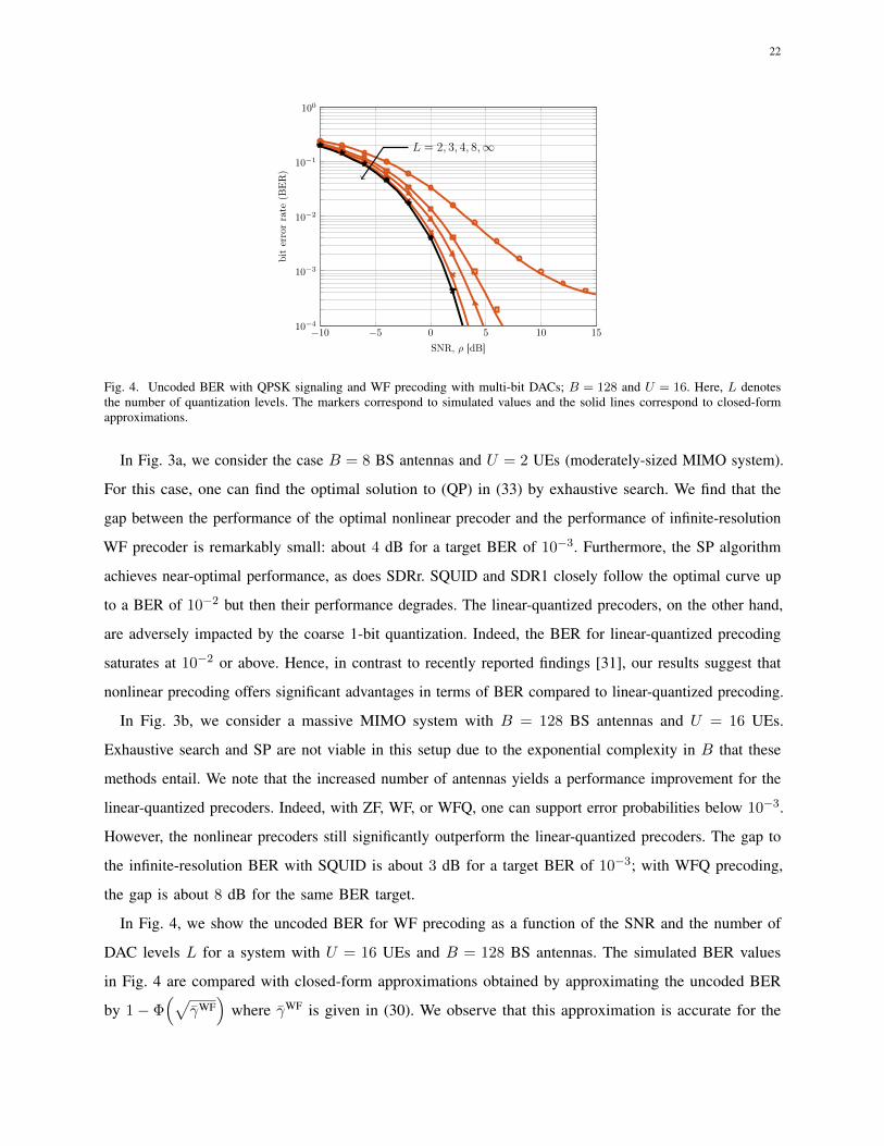
Fig. 4. Uncoded BER with QPSK signaling and WF precoding with multi-bit DACs; B = 128 and U = 16. Here, L denotesthe number of quantization levels. The markers correspond to simulated values and the solid lines correspond to closed-formapproximations.
In Fig. 3a, we consider the case B = 8 BS antennas and U = 2 UEs (moderately-sized MIMO system).
For this case, one can find the optimal solution to (QP) in (33) by exhaustive search. We find that the
gap between the performance of the optimal nonlinear precoder and the performance of infinite-resolution
WF precoder is remarkably small: about 4 dB for a target BER of 10−3. Furthermore, the SP algorithm
achieves near-optimal performance, as does SDRr. SQUID and SDR1 closely follow the optimal curve up
to a BER of 10−2 but then their performance degrades. The linear-quantized precoders, on the other hand,
are adversely impacted by the coarse 1-bit quantization. Indeed, the BER for linear-quantized precoding
saturates at 10−2 or above. Hence, in contrast to recently reported findings [31], our results suggest that
nonlinear precoding offers significant advantages in terms of BER compared to linear-quantized precoding.
In Fig. 3b, we consider a massive MIMO system with B = 128 BS antennas and U = 16 UEs.
Exhaustive search and SP are not viable in this setup due to the exponential complexity in B that these
methods entail. We note that the increased number of antennas yields a performance improvement for the
linear-quantized precoders. Indeed, with ZF, WF, or WFQ, one can support error probabilities below 10−3.
However, the nonlinear precoders still significantly outperform the linear-quantized precoders. The gap to
the infinite-resolution BER with SQUID is about 3 dB for a target BER of 10−3; with WFQ precoding,
the gap is about 8 dB for the same BER target.
In Fig. 4, we show the uncoded BER for WF precoding as a function of the SNR and the number of
DAC levels L for a system with U = 16 UEs and B = 128 BS antennas. The simulated BER values
in Fig. 4 are compared with closed-form approximations obtained by approximating the uncoded BER
by 1− Φ(√
γWF)
where γWF is given in (30). We observe that this approximation is accurate for the

23
0 0.1 0.2 0.3 0.4 0.5 0.6 0.7 0.8 0.9 110−4
10−3
10−2
10−1
100
channel-estimation error, ε
bit
erro
rra
te(B
ER
)
MRTZFWFWFQSDR1SDRrSQUIDWF (inf. res.)
Fig. 5. Uncoded BER with QPSK signaling for 1-bit DACs as a function of the channel-estimation error, ε.
entire range of SNR values. We further observe that low BER probabilities can be attained with very
coarse DACs. Interestingly, by only adding a zero-level in the DACs (so that L = 3), the performance is
drastically improved compared to the 1-bit case (L = 2). Furthermore, with only 3-bit DACs (L = 8) the
performance gap to the infinite-resolution case is negligible. This suggests that it is possible to significantly
reduce the number of bits in the high-resolution DACs used in today’s systems.
B. Robustness to Channel-Estimation Errors
So far, we have assumed that the BS has access to perfect CSI. In this section we shall relax this
assumption to investigate the robustness of the developed algorithms to channel estimation errors. More
specifically, we shall assume that the BS has access to a noisy version of H modelled as
H =√
1− εH +√εZ. (60)
Here, ε ∈ [0, 1] and Z has CN (0, 1) entries. We refer to ε as the channel-estimation error: ε = 0 corresponds
to perfect CSI and ε = 1 corresponds to no CSI; intermediate values corresponds to partial CSI.
In Fig. 5, we show, for the 1-bit case, the uncoded BER with QPSK signaling as a function of the
channel-estimation error ε for a system with B = 128 BS antennas and U = 16 UEs. Interestingly, the
nonlinear precoders still outperform the linear-quantized precoders for ε ≤ 0.5. This implies that nonlinear
precoders can be used also when only imperfect CSI is available to the BS.
C. Achievable rate
Next, we validate the analytic results on the achievable rate with linear-quantized precoders reported in
Section III by numerical simulations.
24
−10 −5 0 5 10 150
20
40
60
80
100
120
L = 2, 3, 4, 8,∞
SNR, ρ [dB]
Sum
rate
[bit
s/s/
Hz]
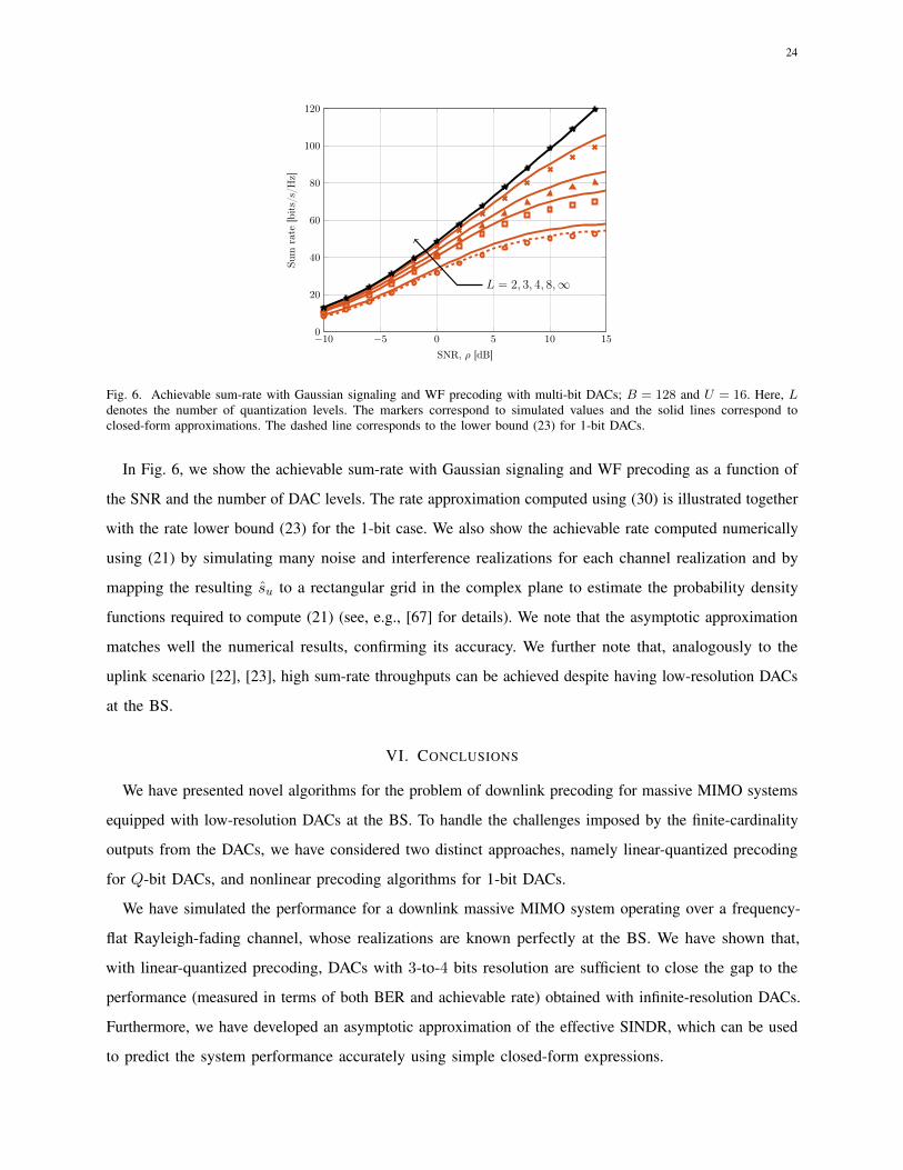
Fig. 6. Achievable sum-rate with Gaussian signaling and WF precoding with multi-bit DACs; B = 128 and U = 16. Here, Ldenotes the number of quantization levels. The markers correspond to simulated values and the solid lines correspond toclosed-form approximations. The dashed line corresponds to the lower bound (23) for 1-bit DACs.
In Fig. 6, we show the achievable sum-rate with Gaussian signaling and WF precoding as a function of
the SNR and the number of DAC levels. The rate approximation computed using (30) is illustrated together
with the rate lower bound (23) for the 1-bit case. We also show the achievable rate computed numerically
using (21) by simulating many noise and interference realizations for each channel realization and by
mapping the resulting su to a rectangular grid in the complex plane to estimate the probability density
functions required to compute (21) (see, e.g., [67] for details). We note that the asymptotic approximation
matches well the numerical results, confirming its accuracy. We further note that, analogously to the
uplink scenario [22], [23], high sum-rate throughputs can be achieved despite having low-resolution DACs
at the BS.
VI. CONCLUSIONS
We have presented novel algorithms for the problem of downlink precoding for massive MIMO systems
equipped with low-resolution DACs at the BS. To handle the challenges imposed by the finite-cardinality
outputs from the DACs, we have considered two distinct approaches, namely linear-quantized precoding
for Q-bit DACs, and nonlinear precoding algorithms for 1-bit DACs.
We have simulated the performance for a downlink massive MIMO system operating over a frequency-
flat Rayleigh-fading channel, whose realizations are known perfectly at the BS. We have shown that,
with linear-quantized precoding, DACs with 3-to-4 bits resolution are sufficient to close the gap to the
performance (measured in terms of both BER and achievable rate) obtained with infinite-resolution DACs.
Furthermore, we have developed an asymptotic approximation of the effective SINDR, which can be used
to predict the system performance accurately using simple closed-form expressions.

25
Linear-quantized precoders are, however, far from optimal. For the case of 1-bit DACs, we have
shown that the error-rate performance can be significantly improved by allowing for nonlinear precoding
algorithms. For example, we showed that for a system with 128 BS antennas serving 16 UEs, the gap to
infinite-resolution performance is about 3 dB for a target BER of 10−3. Nonlinear precoding, however,
entails increased signal-processing complexity. For small-to-moderate sized systems (e.g., 16 BS antennas
or less), SDR- and SP-based precoders offer near-optimal BER-performance at tolerable complexity. For
massive MIMO systems, SQUID is an efficient and hardware-friendly algorithm to find a near-optimal
solution to the 1-bit quantized precoding problem.
APPENDIX A
PROOF OF THEOREM 2
Let z = Ps ∈ CB . It follows from Theorem 1 that the covariance matrices Cxz = Es
[xzH
]and Czz = Es
[zzH
]are related as follows:
Cxz = GCzz (61)
where G is a B ×B diagonal matrix with
[G]b,b =1
σ2b
E[Q(zb)z∗b ] (62)
where zb = [z]b and σ2b = E
[|zb|2
]for b = 1, . . . , B. Note now that
Czz = Es
[zzH
]= PEs
[ssH
]PH = PPH . (63)
It follows from (61) that we can write the quantized signal as x = Gz + d, where the distortion d is
uncorrelated with z. Indeed, note that
Es
[dzH
]= Es
[(x−Gz)zH
]= Cxz −GCzz = 0B×B (64)
where the last equality follows from (61). We next evaluate (62). Note that, since the real and imaginary
components of the symbol vector s are independent and identically distributed, so are the real and
imaginary components of the precoded vector z. Therefore, it holds that E[Q(zb)z∗b ] = 2E[Q(z)z], where
we have introduced the random variable z ∼ N (0, σ2b/2). For a uniform DAC, the quantizer-mapping
function can be expressed as
Q(z) =α∆
2(1− L) + α∆
L−1∑i=1
1[∆(i−L
2 ),∞)(z). (65)
26
Hence, we have that
[G]b,b =2α∆
σ2b
L−1∑i=1
∫ ∞∆(i−L
2 )
z√πσ2
b
exp
(− z
2
σ2b
)dz =
α∆√πσ2
b
L−1∑i=1
exp
(−∆2
σ2b
(i− L
2
)2). (66)
The desired result (14) follows from (66) by using that σ2b = [PPH ]b,b.
APPENDIX B
PROOF OF THEOREM 4
We start by rewriting the proximal operator in (56) as
u = arg minx∈RN , α∈R
λα2 +1
2‖x− y‖22 subject to x2
k ≤ α2, k = 1, . . . , N (67)
and use the Karush-Kuhn-Tucker (KKT) conditions [58] to compute its solution. The Lagrangian of the
optimization problem in (67) is given by
L(x, α,u) = λα2 +1
2‖x− y‖22 +
N∑k=1
uk(x2i − α2) (68)
which yields the following two stationarity conditions:
λ−N∑k=1
ui = 0 (69)
xk − yk + 2xkuk = 0, k = 1, . . . , N. (70)
The stationarity condition (70) reveals that xk = yk/(1 + 2uk), which implies that if uk = 0, then xk = yk.
Complementary slackness yields uk(x2k − α2
k) = 0, which implies that if uk 6= 0, then x2k = α2 for a
given k. Hence the values of xk must either be |xk| = α or xk = yk so that |xk| < α. In words, the
proximal operator in (67) clips to xk = sgn(yk)α the values yk whose magnitude exceeds α and leaves
the remaining values unaffected. Hence, we only need to determine the optimal clipping threshold α∗ > 0.
Assume xk 6= 0 without loss of generality (in the case yk = 0, we have xk = 0). Then, the stationarity
condition in (70) reveals that uk = 12
(ykxk− 1). Together with the stationarity condition (69), we have
N∑k=1
uk =1
2
N∑k=1
(ykxk− 1
)= λ (71)
which implies that
N∑k=1
ykxk
= 2λ+N. (72)

27
We now partition the indices k = 1, . . . , N into two disjoint sets Ω and Ωc, The set Ω contains the indices
of the entries yk for which |yk| ≥ α; the set Ωc contains the indices of the entries uk for which |yk| < α.
Since xk = sgn(yk)α for k ∈ Ω and xk = yk for k ∈ Ωc, it follows from (72) that
∑k∈Ω
|yk|α
+∑k∈Ωc
1 = 2λ+N. (73)
Hence,
∑k∈Ω
|yk|α
= 2λ+N − |Ωc| = 2λ+ |Ω|. (74)
We see from (74) that the clipping threshold α must satisfy
α =
∑k∈Ω |yk|
2λ+ |Ω| . (75)
To solve (67), it is convenient to sort the values |yk| in descending order. Specifically, let us denote these
values by r1 ≥ r2 ≥ · · · ≥ rN . Then one computes α` =∑`
k=1 rk/(2λ + `) for ` = 1, 2, . . . , N and
chooses α∗ as the only α` that satisfies r`+1 < α` ≤ r`. Simple algebraic manipulations reveal that this
is equivalent to setting α∗ = max` α`. We then use α∗ to perform element-wise clipping. Algorithm 1
implements exactly this procedure in a computationally efficient manner.
REFERENCES
[1] F. Rusek, D. Persson, B. Kiong, E. G. Larsson, T. L. Marzetta, O. Edfors, and F. Tufvesson, “Scaling up MIMO: Oppurtunities
and challenges with very large large arrays,” IEEE Signal Process. Mag., vol. 30, no. 1, pp. 40–60, Jan. 2013.
[2] E. G. Larsson, F. Tufvesson, O. Edfors, and T. L. Marzetta, “Massive MIMO for next generation wireless systems,” IEEE
Commun. Mag., vol. 52, no. 2, pp. 186–195, Feb. 2014.
[3] L. Lu, G. Ye Li, A. L. Swindlehurst, A. Ashikhmin, and R. Zhang, “An overview of massive MIMO: Benefits and challenges,”
IEEE J. Sel. Topics Signal Process., vol. 8, no. 5, pp. 742–758, Oct. 2014.
[4] G. Caire and S. Shamai (Shitz), “On the achievable throughput of a multiantenna Gaussian broadcast channel,” IEEE Trans.
Inf. Theory, vol. 49, no. 7, pp. 1691–1706, Jul. 2003.
[5] W. Yu and J. M. Cioffi, “Sum capacity of Gaussian vector broadcast channels,” IEEE Trans. Inf. Theory, vol. 50, no. 9, pp.
1875–1892, Sep. 2004.
[6] S. Viswanath, N. Jindal, and A. Goldsmith, “Duality, achievable rates, and sum-rate capacity of Gaussian MIMO broadcast
channels,” IEEE Trans. Inf. Theory, vol. 49, no. 10, pp. 2658–2668, Oct. 2003.
[7] P. Viswanath and D. Tse, “Sum capacity of the vector Gaussian broadcast channel and uplink–downlink duality,” IEEE
Trans. Inf. Theory, vol. 49, no. 8, pp. 1912–1921, Aug. 2003.
[8] M. H. Costa, “Writing on dirty paper,” IEEE Trans. Inf. Theory, vol. 29, no. 3, pp. 439–441, May 1983.
[9] R. D. Wesel and J. M. Cioffi, “Achievable rates for Tomlinson–Harashima precoding,” IEEE Trans. Inf. Theory, vol. 44,
no. 2, pp. 824–831, Mar. 1998.
28
[10] C. Windpassinger, R. F. H. Fischer, T. Vencel, and J. B. Huber, “Precoding in multiantenna and multiuser communications,”
IEEE Trans. Wireless Commun., vol. 3, no. 4, pp. 1305–1316, Jul. 2004.
[11] C. Windpassinger, R. F. H. Fischer, and J. B. Huber, “Lattice-reduction-aided broadcast precoding,” IEEE Trans. Commun.,
vol. 52, no. 12, pp. 2057–2060, Dec. 2004.
[12] B. M. Hochwald, C. B. Peel, and A. L. Swindlehurst, “A vector-perturbation technique for near-capacity multiantenna
multiuser communication—Part II: Perturbation,” IEEE Trans. Commun., vol. 53, no. 3, pp. 537–544, Mar. 2005.
[13] H. Yang and T. L. Marzetta, “Performance of conjugate and zero-forcing beamforming in large-scale antenna systems,”
IEEE J. Sel. Areas Commun., vol. 31, no. 2, pp. 172–179, Feb. 2013.
[14] H. Q. Ngo, E. G. Larsson, and T. L. Marzetta, “Massive MU-MIMO downlink TDD systems with linear precoding and
downlink pilots,” in Proc. Allerton Conf. Commun., Contr., Comput., Monticello, IL, Oct. 2013.
[15] C. Studer, M. Wenk, and A. Burg, “MIMO transmission with residual transmit-RF impairments,” in Int. ITG Workshop on
Smart Antennas (WSA), Bremen, Germany, Feb. 2010, pp. 189–196.
[16] U. Gustavsson, C. Sanchéz-Perez, T. Eriksson, F. Athley, G. Durisi, P. Landin, K. Hausmair, C. Fager, and L. Svensson,
“On the impact of hardware impairments on massive MIMO,” in Proc. IEEE Global Telecommun. Conf. (GLOBECOM),
Austin, TX, Dec. 2014, pp. 294–300.
[17] X. Zhang, M. Matthaiou, M. Coldrey, and E. Björnson, “Impact of residual transmit RF impairments on training-based
MIMO systems,” IEEE Trans. Commun., vol. 63, no. 8, pp. 2899–2911, Aug. 2015.
[18] F. Athley, G. Durisi, and U. Gustavsson, “Analysis of massive MIMO with hardware impairments and different channel
models,” in European Conf. Ant. Prop. (EUCAP), Lisbon, Portugal, Apr. 2015.
[19] R. H. Walden, “Analog-to-digital converter survey and analysis,” IEEE J. Sel. Areas Commun., vol. 17, no. 4, pp. 539–550,
Apr. 1999.
[20] B. Murmann, “ADC performance survey 1997-2015.” [Online]. Available: http://web.stanford.edu/~murmann/adcsurvey.html
[21] C. Risi, D. Persson, and E. G. Larsson, “Massive MIMO with 1-bit ADC,” Apr. 2014. [Online]. Available:
http://arxiv.org/abs/1404.7736
[22] S. Jacobsson, G. Durisi, M. Coldrey, U. Gustavsson, and C. Studer, “One-bit massive MIMO: Channel estimation and
high-order modulations,” in Proc. IEEE Int. Conf. Commun. Workshop (ICCW), London, U.K., June 2015, pp. 1304–1309.
[23] Y. Li, C. Tao, G. Seco-Granados, A. Mezghani, A. L. Swindlehurst, and L. Liu, “Channel estimation and performance
analysis of one-bit massive MIMO systems,” Sep. 2016. [Online]. Available: https://arxiv.org/abs/1609.07427
[24] C. Mollén, J. Choi, E. G. Larsson, and R. W. Heath Jr., “Performance of the wideband massive uplink MIMO with one-bit
ADCs,” Feb. 2016. [Online]. Available: https://arxiv.org/abs/1602.07364
[25] C. Studer and G. Durisi, “Quantized massive MU-MIMO-OFDM uplink,” IEEE Trans. Commun., vol. 64, no. 6, pp.
2387–2399, Jun. 2016.
[26] C. Studer and E. G. Larsson, “PAR-aware large-scale multi-user MIMO-OFDM downlink,” IEEE J. Sel. Areas Commun.,
vol. 31, no. 2, pp. 303–313, Feb. 2013.
[27] S. K. Mohammed and E. G. Larsson, “Per-antenna constant envelope precoding for large multi-user MIMO systems,” IEEE
Trans. Commun., vol. 61, no. 3, pp. 1059–1071, Mar. 2013.
[28] ——, “Constant-envelope multi-user precoding for frequency-selective massive MIMO systems,” IEEE Commun. Lett.,
vol. 2, no. 5, pp. 547–550, Oct. 2013.
[29] A. Mezghani, R. Ghiat, and J. A. Nossek, “Transmit processing with low resolution D/A-converters,” in Proc. IEEE Int.
Conf. Electron., Circuits, Syst. (ICECS), Yasmine Hammamet, Tunisia, Dec. 2009, pp. 683–686.
29
[30] R. D. J. Guerreiro and P. Montezuma, “Use of 1-bit digital-to-analogue converters in massive MIMO systems,” IEEE
Electron. Lett., vol. 52, no. 9, pp. 778–779, Apr. 2016.
[31] A. K. Saxena, I. Fijalkow, and A. L. Swindlehurst, “On one-bit quantized ZF precoding for the multiuser massive MIMO
downlink,” in IEEE Sensor Array and Multichannel Signal Process. Workshop (SAM), Rio de Janeiro, Brazil, Jul. 2016.
[32] O. B. Usman, H. Jedda, A. Mezghani, and J. A. Nossek, “MMSE precoder for massive MIMO using 1-bit quantization,” in
Proc. IEEE Int. Conf. Acoust., Speech, Signal Process. (ICASSP), Shanghai, China, Mar. 2016, pp. 3381–3385.
[33] E. Björnson, M. Bengtsson, and B. Ottersten, “Optimal multiuser transmit beamforming: A difficult problem with a simple
solution structure,” IEEE Signal Process. Mag., vol. 31, no. 4, pp. 142–148, Jul. 2014.
[34] E. Björnson and E. Jorswieck, “Optimal resource allocation in coordinated multi-cell systems,” Foundations and Trends in
Communications and Information Theory, vol. 9, no. 2-3, pp. 113–381, 2013.
[35] S. S. Christensen, E. C. Agarwal, and J. M. Cioffi, “Weighted sum-rate maximization using weighted MMSE for MIMO-BC
beamforming design,” IEEE Trans. Wireless Commun., vol. 7, no. 12, pp. 4792–4799, Dec. 2008.
[36] M. Joham, W. Utschick, and J. A. Nossek, “Linear transmit processing in MIMO communications systems,” IEEE Trans.
Signal Process., vol. 53, no. 8, pp. 2700–2712, Aug. 2005.
[37] S. Shi, M. Schubert, and H. Boche, “Downlink MMSE transceiver optimization for multiuser MIMO systems: Duality and
sum-MSE minimization,” IEEE Trans. Signal Process., vol. 55, no. 11, pp. 5436–5446, Nov. 2007.
[38] J. J. Bussgang, “Crosscorrelation functions of amplitude-distorted Gaussian signals,” Res. Lab. Elec., Cambridge, MA, Tech.
Rep. 216, Mar. 1952.
[39] D. Hui and D. L. Neuhoff, “Asymptotic analysis of optimal fixed-rate uniform scalar quantization,” IEEE Trans. Inf. Theory,
vol. 47, no. 3, pp. 957–977, Mar. 2001.
[40] N. Al-Dhahir and J. M. Cioffi, “On the uniform ADC bit precision and clip level computation for a Gaussian signal,” IEEE
Trans. Signal Process., vol. 44, no. 2, pp. 434–438, Feb. 1996.
[41] H. E. Rowe, “Memoryless nonlinearities with Gaussian inputs: Elementary results,” Bell Labs Tech. J., vol. 61, no. 7, pp.
1519–1525, Sep. 1982.
[42] H. Q. Ngo and E. G. Larsson, “No downlink pilots are needed in TDD massive MIMO,” Sep. 2016. [Online]. Available:
https://arxiv.org/abs/1606.02348
[43] D. M. Arnold, H.-A. Loeliger, P. O. Vontobel, A. Kavcic, and W. Zeng, “Simulation-based computation of information
rates for channels with memory,” IEEE Trans. Inf. Theory, vol. 52, no. 8, pp. 3498–3508, Aug. 2006.
[44] J. Scarlett, “Reliable communication under mismatched decoding,” Ph.D. dissertation, University of Cambridge, U.K., Jun.
2014.
[45] A. Lapidoth, “Mismatched decoding and the multiple access channel,” IEEE Trans. Inf. Theory, vol. 42, no. 5, pp. 1439–1452,
Sep. 1996.
[46] J. H. Van Vleck and D. Middleton, “The spectrum of clipped noise,” Proc. IEEE, vol. 54, no. 1, pp. 2–19, Jan. 1966.
[47] G. Jacovitti and A. Neri, “Estimation of the autocorrelation function of complex Gaussian stationary processes by amplitude
clipped signals,” IEEE Trans. Inf. Theory, vol. 40, no. 1, pp. 239–245, Jan. 1994.
[48] R. Coulliet and M. Debbah, Random Matrix Methods for Wireless Communications. Cambridge: Cambridge Univ. Press,
2011.
[49] S. Wagner, R. Coulliet, M. Debbah, and D. T. M. Slock, “Large system analysis of linear precoding in correlated MISO
broadcast channels under limited feedback,” IEEE Trans. Inf. Theory, vol. 58, no. 7, pp. 4509–4537, Jul. 2012.
[50] J. Hoydis, S. ten Brink, and M. Debbah, “Massive MIMO in the UL/DL of cellular networks: How many antennas do we
need?” IEEE J. Sel. Areas Commun., vol. 31, no. 2, pp. 160–171, Feb. 2013.

30
[51] E. Agrell, T. Eriksson, A. Vardy, and K. Zeger, “Closest point search in lattices,” IEEE Trans. Inf. Theory, vol. 48, no. 8,
pp. 2201–2214, Aug. 2002.
[52] U. Fincke and M. Pohst, “Improved methods for calculating vectors of short length in a lattice, including a complexity
analysis,” Math. Comput., vol. 44, no. 170, pp. 463–471, Apr. 1985.
[53] S. Verdú, “Computational complexity of multiuser detection,” Algorithmica, vol. 4, no. 1, pp. 303–312, 1989.
[54] Z.-Q. Luo, W.-K. Ma, A. M.-C. So, Y. Ye, and S. Zhang, “Semidefinite relaxation of quadratic optimization problems,”
IEEE Signal Process. Mag., vol. 27, no. 3, pp. 20–34, May 2010.
[55] P. H. Tan and L. Rasmussen, “The application of semidefinite programming for detection in CDMA,” IEEE J. Sel. Areas
Commun., vol. 19, no. 8, pp. 1442–1449, Aug. 2001.
[56] M. Bengtsson and B. Ottersten, “Optimal downlink beamforming using semidefinite optimization,” in Allerton Conf.
Commun., Contr., Comput., Monticello, IL, Sep. 1999.
[57] N. D. Sidiropoulos, T. N. Davidson, and Z.-Q. Luo, “Transmit beamforming for physical-layer multicasting,” IEEE Trans.
Signal Process., vol. 54, no. 6, pp. 2239–2251, Jun. 2006.
[58] S. Boyd and L. Vandenberghe, Convex Optimization. New York, NY, USA: Cambridge Univ. Press, 2004.
[59] O. Castañeda, T. Goldstein, and C. Studer, “Data detection in large multi-antenna wireless systems via approximate
semidefinite relaxation,” Sep. 2016. [Online]. Available: https://arxiv.org/abs/1609.01797
[60] N. Parikh and S. Boyd, Proximal algorithms. Now Publishers, 2013.
[61] T. Goldstein, C. Studer, and R. Baraniuk, “A field guide to forward-backward splitting with a FASTA implementation,” Feb.
2016. [Online]. Available: https://arxiv.org/abs/1411.3406
[62] P. L. Lions and B. Mercier, “Splitting algorithms for the sum of two nonlinear operators,” SIAM J. Numer. Anal., vol. 16,
no. 6, pp. 964–979, Dec. 1979.
[63] J. Eckstein and D. P. Bertsekas, “On the Douglas-Rachford splitting method and the proximal point algorithm for maximal
monotone operators,” Math. Programming, vol. 55, pp. 293–318, Apr. 1992.
[64] C. Studer and H. Bölcskei, “Soft-input soft-output single tree-search sphere decoding,” IEEE Trans. Inf. Theory, vol. 56,
no. 10, pp. 4827–4842, Oct. 2010.
[65] J. Jaldén and B. Ottersten, “On the complexity of sphere decoding in digital communications,” IEEE Trans. Signal Process.,
vol. 53, no. 4, pp. 1474–1484, Apr. 2005.
[66] D. Seethaler, J. Jaldén, C. Studer, and H. Bölcskei, “On the complexity distribution of sphere decoding,” IEEE Trans. Inf.
Theory, vol. 57, no. 9, pp. 5754–5768, Sep. 2011.
[67] S. Jacobsson, G. Durisi, M. Coldrey, U. Gustavsson, and C. Studer, “Throughput analysis of massive MIMO uplink with
low-resolution ADCs,” Jul. 2016. [Online]. Available: https://arxiv.org/abs/1602.01139


![[EURASIP 2013] Linear Precoding in Distributed MIMO Systems With Partial CSIT](https://static.cupdf.com/doc/110x72/577cd2281a28ab9e78953348/eurasip-2013-linear-precoding-in-distributed-mimo-systems-with-partial-csit.jpg)