QUALITY–QUANTITY DECOMPOSITION OF INCOME ELASTICITYOF U.S. HOSPITAL CARE EXPENDITURE USING STATE-LEVEL
PANEL DATA†
WEIWEI CHENa, ALBERT OKUNADEa,* and GREGORY G. LUBIANIb
aUniversity of Memphis, Economics, Memphis, TN, USAbXavier University, Health Services Administration, Cincinnati, OH, USA
SUMMARY
Economic theory suggests that income growth could lead to changes in consumption quantity and quality as the spending ona commodity changes. Similarly, the volume and quality of healthcare consumption could rise with incomes because ofdemographic changes, usage of innovative medical technologies, and other factors. Hospital healthcare spending is the largestcomponent of aggregate US healthcare expenditures. The novel contribution of our paper is estimating and decomposing theincome elasticity of hospital care expenditures (HOCEXP) into its quantity and quality components. By using a 1999–2008panel dataset of the 50 US states, results from the seemingly unrelated regressions model estimation reveal the income elasticityof HOCEXP to be 0.427 (std. error=0.044), with about 0.391 (calculated std. error=0.044) arising from care qualityimprovements and 0.035 (std. error=0.050) emanating from the rise in usage volume. Our novel research findings suggestthe following: (i) the quantity part of hospital expenditure is inelastic to income change; (ii) almost the entire income-induced rise in hospital expenditure comes from care quality changes; and (iii) the 0.427 income elasticity of HOCEXP, thelargest component of total US healthcare expenditure, makes hospital care a normal commodity and a much stronger technicalnecessity than aggregate healthcare. Policy implications are discussed. Copyright © 2013 John Wiley & Sons, Ltd.
Received 17 September 2012; Revised 20 June 2013; Accepted 16 July 2013
JEL Classification: I1
KEY WORDS: quantity and quality decomposition; income elasticity; hospital care expenditure; seemingly unrelatedregressions estimates; US state-level panel data
1. INTRODUCTION
The US national healthcare expenditures (HEXP) have risen substantially over the past few decades. Although its
growth rate slowed during the 2007–2009 economic recession and the currently early recovery phase of the
business cycle, total HEXP in 2010 surprisingly reached $2.6 trillion and accounted for 17.9% of the GDP, or
$8402 per person (Martin et al., 2012). The persistently high US per capita HEXP remains the largest compared
to any country in the world. Despite several decades of multi-pronged policy interventions that target cost contain-
ments and quality improvements, healthcare economics investigations of the determinants of HEXP and the roles
that the multi-dimensioned care quality may play continue to proliferate for their potential implications on policy.
Among the large number of works in this area, publications on the determinants of HEXP debating the
magnitude and inference on the nature of healthcare good from the estimated income elasticities account for a large
part of the discussion. Although the income elasticity of HEXP has important policy implications, this current
investigation advances beyond estimation of the income elasticity by estimating a parsimonious model for
*Correspondence to: Department of Economics, University of Memphis, Memphis, TN 38152, USA. E-mail: [email protected]†This manuscript does not require approval of an ethics or human subjects committee.
Copyright © 2013 John Wiley & Sons, Ltd.
HEALTH ECONOMICSHealth Econ. (2013)Published online in Wiley Online Library (wileyonlinelibrary.com). DOI: 10.1002/hec.2986
decomposing the elasticity of hospital care expenditure, the largest component of total US healthcare spending,
into its quantity and quality aspects. The decomposition idea was inspired by a classic work (Hicks and Johnson,
1968) in agricultural economics on the nature of the income elasticity of food demand. There, the authors used a
simplified model to determine the composition of income elasticity of food expenditures in terms of quantity
changes, measured as calories in the diet, and quality variations, measured as the ratio of calories from non-starchy
foods to calories from starchy foods. Similarly, the quantity (i.e., volume) and quality of healthcare consumed
could rise as incomes grow because of both greater demand from population expansion and aging, and also the
discovery and widespread adoption of innovative treatment technologies. Methodologically, we glean and modify
further ideas from Engel curves modeling in agricultural economics on the relationship among expenditure, price,
quality, and quantity. Using a panel dataset of 50 US states on hospital expenditures for the 1999–2008 period, we
propose in this study a two-equation, seemingly unrelated regressions (SUR) system for estimating the hospital
expenditure model useful for decomposing the resulting income elasticity into its quantity and quality components.
Hospital care expenditure (HOCEXP), and not total HEXP predominantly studied in past research, is the
current study focus for many reasons. First, the aggregate HEXP is a largely heterogeneous construct comprising
expenditures on hospital care (inpatient and outpatient), physicians and clinical services, prescriptions, nursing
homes, and others. In effect, income elasticities estimates are likely to vary by expenditure category types and
providers (Costa-Font et al., 2011). Second, the various expenditure sub-categories would require separate
quantity (volume) and quality measures in order to properly decompose and obtain theoretically consistent and
robust expenditure-specific income elasticities. Consequently, for a sound quality and quantity decomposition,
focusing on a major expenditure category and using appropriate quality and quantity measures should enhance
the reliability and applicability of study findings. Finally, HOCEXP is the largest share of total HEXP in the
USA, and the relevant data for econometric model estimation tend to be more readily available when compared
with those of the other components of aggregate HEXP. During 2010, the US overall spending for hospital services
reached $814.0 billion and accounted for 31.4% of total health spending and 5.6% of GDP.1Given the continuing
rise in HEXP, it is timely to investigate whether quality-based or quantity-based aspects of the growth in this major
HEXP category should be policy targets for tighter cost containments. An additional rationale for focusing on
HOCEXP is the recent (2012) US Supreme Court ruling upholding constitutionality of the multiple provisions
in the 2010 Affordable Care Act (ACA), most notably the individual mandate. Moreover, although the forced
expansion of Medicaid was rejected, it left the door open for states to voluntarily participate. Although initially
resisting the expansion, many states have recently begun to alter that stance and are exploring policy options that
would broaden healthcare access for a greater share of low-income earners. The expanding insurance coverage, or
financial gain, favors hospitals, as it is projected to reduce their uncompensated care significantly and promote the
acquisitions of physician practices to secure sustainable competitive advantages, augment physician recruitment
strategies, and form accountable care organizations (Glenn, 2013). All of these portendHOCEXP growth for years
to come, especially after the full implementation of the ACA in 2015.
To our knowledge, this current study represents the first attempt to decompose the income elasticity of
HOCEXP into its quality and quantity components. The US hospital sector is dominated by not-for-profit
providers whose utility maximizing behavioral tendencies depend on the amount of quantity and quality of care
provided, subject to a constraint (Newhouse, 1970). Today, the hospital sub-sector continues to play a central
role in health systems across all countries (Sloan and Hsieh, 2012). Because healthcare economics research
touching on quality and value are at the core of policy reform efforts for providers, payers, and consumers,
the income elasticity of HOCEXP estimation and decomposition strategy advanced and implemented here
has replication potentials for investigating the other components of aggregate healthcare (and non-health
commodity) expenditure for which quality progression occurs in tandem with quantity change as incomes rise.
The rest of this paper proceeds as follows. Section 2 reviews the literature, Section 3 motivates the theoretical
model and empirical strategy along with the data for estimating income elasticity and its quality–quantity decompo-
sition, Section 4 focuses on the estimation results, and Section 5 concludes with the summary and implications.
1Calculated on the basis of Exhibit 1 by Martin et al., 2012.
W. CHEN ET AL.
Copyright © 2013 John Wiley & Sons, Ltd. Health Econ. (2013)
DOI: 10.1002/hec

2. LITERATURE REVIEW
2.1. Income elasticity of healthcare expenditures
Dating back to the seminal paper by Newhouse (1977), income is consistently one of the core determinants of
aggregate HEXP. The income elasticity of HEXP is important because of its policy implications for whether the
healthcare commodity is a technical necessity or luxury. The magnitude of income elasticity of HEXP would
differ, depending on the data aggregation level being modeled. Getzen (2000) concluded that individual data
income elasticities are close to zero, whereas national HEXP elasticities are commonly greater than one. The
intuition is that health status plays an important role in individual healthcare spending as this effect attenuates
at the macro levels. Moreover, Paluch et al. (2012) indicated that the aggregate elasticity can be very different
from the mean of individual elasticities. The difference depends on the heterogeneity of the population and is
quantified by a covariance term, and the magnitude of this difference varies from commodity to commodity.
Even at the same data aggregation level, the income elasticities can be very different depending on other
attributes of the data and research methodology. This is the case for empirical papers using state-level data.
Surprisingly, the estimated state-level income elasticities of HEXP in the existing literature range from near
0 to 1 or more (Di Matteo, 2003). Ringel et al. (2002) and Chernew and Newhouse (2012) claimed that studies
using long time-series or panel data tend to report higher income elasticities. In general, the reported income
elasticity estimates in past studies appear sensitive to the data structure (cross-sectional, time-series, and panel),
regression model specification (functional forms, included and excluded independent variables), and model
estimation methods. Recently, Costa-Font et al. (2011) used bias-corrected meta-regression analysis to cast
doubt on the luxury goods hypothesis in aggregate data health expenditure models. Their study placed robust
estimates of income elasticities of HEXP in the 0.4–0.8 range.
Published studies on the numerical magnitude of the income elasticity of HOCEXP, the largest component
of HEXP in the US, are extremely rare. Acemoglu et al. (2012) estimated the income elasticity of HOCEXP by
instrumenting for local area income with time-series variation in global oil prices interacted with cross-sectional
variation in the oil reserves in different areas of the southern USA. The estimated state-level income elasticity
using gross state product as income and for the whole US geographic sample was 0.568. Newhouse and Phelps
(1976) estimated the US income elasticity of hospital care utilization at the individual level. The wage income
elasticity of length of hospital stay was roughly 0.10 on the basis of the two-stage least squares regression
estimation method.
2.2. Quality in healthcare expenditures
Measuring healthcare quality is very difficult, because it is a multi-dimensional concept that encompasses
contractable and non-contractable aspects (Sloan and Hsieh, 2012). Although there is no lack of hospital-level
or disease-specific quality measures, no single commonly accepted quality indicator is capable of capturing all
of the many dimensions of care quality. Copnell et al. (2009) identified 383 discrete indicators currently in use
to measure the care quality provided by hospitals from 22 sources of organizations or projects. They found
27.2% of the indicators as relevant hospital-wide, 26.1% to be applicable to surgical patients, and 46.7%
applicable to non-surgical specialties, departments, or diseases. Processes of care were measured by 54.0%
of the indicators, and outcomes by 38.9%. Safety and effectiveness were the domains most frequently
represented, with relatively few indicators measuring the other dimensions. They concluded that despite the
large number of available indicators, significant gaps in measurement and implementations persist. Whether
existing indicators capture what they purport to measure is yet to be evaluated.
There are various methods for eliciting proxies for quality measures in healthcare, including for hospitals
(see, e.g., Newhouse, 1970; Akin et al., 1995; Grabowski, 2001; Jappelli et al., 2007; Schneider, 2008;
Lichtenberg, 2011). Our paper exploits the relatively less controversial method of modeling quality using the
modified price. For most goods, high quality means a high cost or a high price. Quality is then measured in
QUALITY–QUANTITY DECOMPOSITION OF INCOME ELASTICITY OF HOSPITAL CARE
Copyright © 2013 John Wiley & Sons, Ltd. Health Econ. (2013)
DOI: 10.1002/hec

‘money’ terms. This conceptual method for modeling quality in economics literature (Sloan and Hsieh, 2012) is
detailed in Section 3 of this study.
2.3. Other determinants of healthcare expenditures
Many studies affirm technological change as another primary determinant of healthcare spending growth
(Chernew and Newhouse, 2012). The earliest paper on this is probably that of Schwartz (1987), who applied
the Solow residual method to healthcare spending growth. Newhouse (1992) concluded similarly after control-
ling for more non-technological factors and using data covering a longer period. Smith et al. (2009) found that
changes in medical technology explain 27–48% of the US health spending growth since 1960. Peden and
Freeland (1998) used the insurance coverage level and non-commercial research spending as proxies for
technology and attributed 70% of spending growth to changes in the medical technology. Okunade and Murthy
(2002) utilized total R&D and health R&D spending interchangeably to proxy technological change and found
a statistically significant and stable long-run relationship among per capita real HEXP, per capita real income,
and broad-based R&D expenditures. Some papers use time trends or year fixed effects in their regression
models to control for technological change.
The generosity of health insurance coverage also encourages healthcare spending growth. A commonly used
control for insurance is the percentage of insurance types in the model. Other explanatory variables include
supply-side controls, such as the number of hospital beds, health maintenance organization (HMO) penetration
rates, population health status, demographic characteristics (age, gender, and ethnicities), and regional factors.
More recent papers further include health risk behaviors among the determinants of healthcare spending. Rising
obesity rates are shown to be linked to the rise in medical care spending (Finkelstein et al., 2009). Lichtenberg
(2011) and Cuckler et al. (2011) included the prevalence of obesity and smoking in their models. Lichtenberg
concluded that these two do not appear to influence per capita medical expenditures. Interestingly though,
Cuckler et al. (2011) used the product of the two factors and found it to have a significant effect on healthcare
spending. Our current study includes covariates controlling for many of the factors discussed previously.
2.4. Decomposing the income elasticity of hospital care expenditure
A comprehensive literature search confirms the lack of studies decomposing the income elasticity of total
HEXP or of its sub-categories into quantity and quality components. However, there are some studies
decomposing the expenditure elasticity (with respect to income or other determinants) for commodities other
than healthcare. Hicks and Johnson (1968) estimated the quantity and quality components for income elastic-
ities of demand for food using country level cross-sectional data. They used calories in the diet as the quantity
measure and the ratio of calories from non-starchy foods to calories from starchy foods as the quality measure.
Moreover, other studies in agricultural economics literature on Engel expenditure curves (e.g., Deaton, 1988;
Bils and Klenow, 2001; Gale and Huang, 2007) also yielded some insights into modeling the relationship
between expenditures and income through price, quality, and quantity effects. Archibald and Gillingham (1981)
studied the decomposition of price and income elasticity of demand for gasoline. Gertler (1985) performed a
similar analysis for Medicaid nursing homes. Each nursing home in his paper is solving the optimization problem,
and the derived first order condition is then used to perform the decomposition.
Some past studies decomposed healthcare spending into components different from our current study. For
example, Bradley and Kominski (1992) decomposed the change in average Medicare inpatient costs per case
between 1984 and 1987 into input price inflation, changes in costs with diagnostic-related groups (DRGs),
and changes in case mix across DRGs. Their technology effect was nested in the distribution of cases across
DRGs. Bundorf et al. (2009) and some other investigators decomposed the health spending growth into
quantity growth and price changes. The quality change in these models was presumably excluded or captured
using price changes. Our paper innovates by integrating ideas from past work outside of health economics and
modifying them for application to the healthcare sector in the specific context of the US HOCEXP.
W. CHEN ET AL.
Copyright © 2013 John Wiley & Sons, Ltd. Health Econ. (2013)
DOI: 10.1002/hec

3. EMPIRICAL STRATEGY AND DATA
3.1. Motivating the decomposition model
Our modified income elasticity of HOCEXP decomposition model is inspired by the agricultural economics
literature on Engel curves (Deaton, 1988; Bils and Klenow, 2001; Gale and Huang, 2007) and food demand
(Hicks and Johnson, 1968) models.
We start in Eq. (1) with the identity that expenditures on hospital care, HOCEXP, is equal to price P times
quantity Q.
HOCEXP ≡ P�Q (1)
Quantity Q represents the volume of purchased hospital services, including inpatient and outpatient
services. P is an average price paid for all hospital services used, or a unit value (the ratio of expendi-
tures to quantity purchased). We follow existing literature on Engel curves and assume that ‘quality’
comes into play through the unit value P (i.e., different quality levels due to the heterogeneity of hospital
services would result in different unit values). The unit value can increase either because prices of items
in a fixed basket rise or because different and higher quality (usually more expensive) items are now in
the basket. The former is due to a ‘pure’ price effect, and the latter is because of a shift in the
composition of services toward premium services. We model this relationship using Eq. (2), which states
that the unit value is the product of the price of a fixed basket of services and quality. Denoting hospital
quality of care as v, we can also interpret it as a base price adjusted by quality. Denote the price of a
fixed basket of hospital services as Pf.
P ¼ Pf � v (2)
Plugging Eq. (2) into the HOCEXP Eq. (1), one obtains
HOCEXP ¼ Pf � v �Q (3)
HOCEXP, v, and Q tend to change as income changes. Thus, HOCEXP, v, and Q are functions of
income y. Over a long period, the fixed basket price Pf could be correlated with income too, so Pf is also
assumed to be a function of y. In empirical application, this study also controls for factors other than
income that affect the four variables described previously. Denoting a vector of such factors as X and
X = (Xp, Xv, XQ), where Xp, Xv, and XQ represent the factors that affect Pf, v, and Q, respectively. The
HOCEXP equation can be rewritten as
HOCEXP y;Xð Þ ¼ Pf y;X p
� �
� v y;Xvð Þ �Q y;XQð Þ (4)
Taking the logarithm of both sides of the equation gives
ln HOCEXP y;Xð Þ ¼ lnPf y;Xp
� �
þ lnv y;Xvð Þ þ lnQ y;XQð Þ (5)
Or,
lnHOCEXP y;Xð Þ
Pf y;Xp
� � ¼ ln v y;Xvð Þ þ lnQ y;XQð Þ (6)
The left-hand side in Eq. (6) is simply the log of hospital expenditures adjusted by price index of a fixed
basket of hospital care services.
The rationale for moving Pf(y, Xp) to the left-hand side is that (i) combining HOCEXP and Pf into one-
variable HOCEXP/Pf gives a relation of elasticities among three variables rather than four and (ii) the quality
QUALITY–QUANTITY DECOMPOSITION OF INCOME ELASTICITY OF HOSPITAL CARE
Copyright © 2013 John Wiley & Sons, Ltd. Health Econ. (2013)
DOI: 10.1002/hec
elasticity may be derived if the adjusted expenditure elasticity and quantity elasticity are known. If Pf(y, Xp)
remains on the right-hand side, there exists the need to estimate one more equation to derive the quality
elasticity, but the requisite data on Pf are not available at the state level.
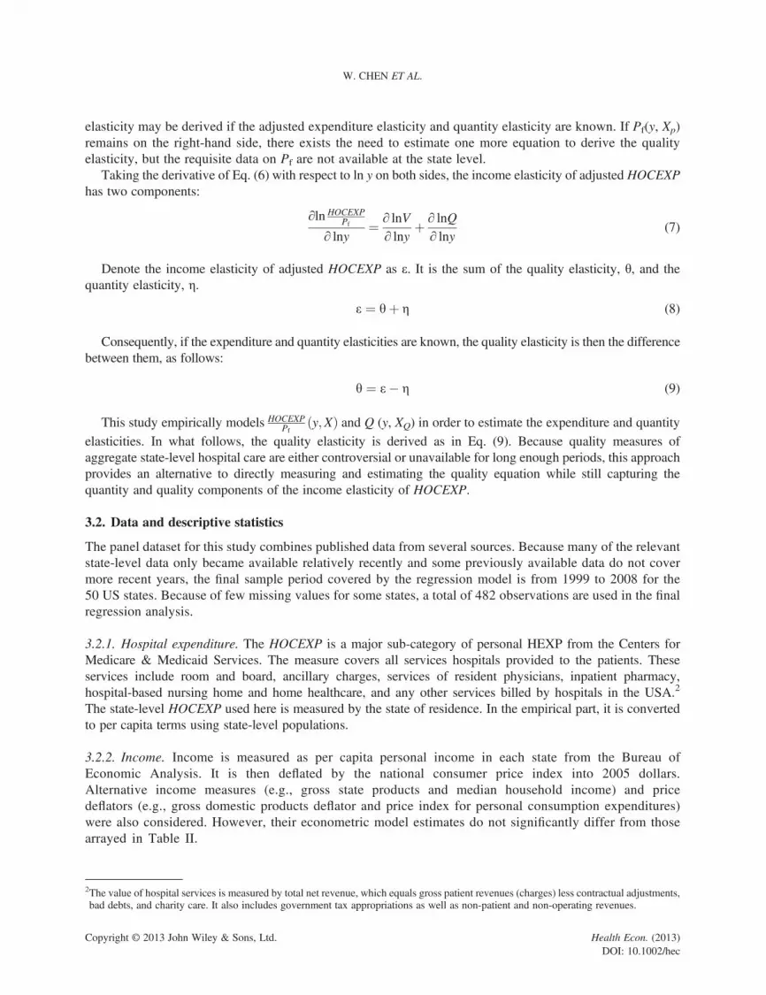
Taking the derivative of Eq. (6) with respect to ln y on both sides, the income elasticity of adjusted HOCEXP
has two components:
∂ln HOCEXPPf
∂ lny¼
∂ lnV
∂ lnyþ
∂ lnQ
∂ lny(7)
Denote the income elasticity of adjusted HOCEXP as ε. It is the sum of the quality elasticity, θ, and the
quantity elasticity, η.
ε ¼ θþ η (8)
Consequently, if the expenditure and quantity elasticities are known, the quality elasticity is then the difference
between them, as follows:
θ ¼ ε� η (9)
This study empirically models HOCEXPPf
y;Xð Þ and Q (y, XQ) in order to estimate the expenditure and quantity
elasticities. In what follows, the quality elasticity is derived as in Eq. (9). Because quality measures of
aggregate state-level hospital care are either controversial or unavailable for long enough periods, this approach
provides an alternative to directly measuring and estimating the quality equation while still capturing the
quantity and quality components of the income elasticity of HOCEXP.
3.2. Data and descriptive statistics
The panel dataset for this study combines published data from several sources. Because many of the relevant
state-level data only became available relatively recently and some previously available data do not cover
more recent years, the final sample period covered by the regression model is from 1999 to 2008 for the
50 US states. Because of few missing values for some states, a total of 482 observations are used in the final
regression analysis.
3.2.1. Hospital expenditure. The HOCEXP is a major sub-category of personal HEXP from the Centers for
Medicare & Medicaid Services. The measure covers all services hospitals provided to the patients. These
services include room and board, ancillary charges, services of resident physicians, inpatient pharmacy,
hospital-based nursing home and home healthcare, and any other services billed by hospitals in the USA.2
The state-level HOCEXP used here is measured by the state of residence. In the empirical part, it is converted
to per capita terms using state-level populations.
3.2.2. Income. Income is measured as per capita personal income in each state from the Bureau of
Economic Analysis. It is then deflated by the national consumer price index into 2005 dollars.
Alternative income measures (e.g., gross state products and median household income) and price
deflators (e.g., gross domestic products deflator and price index for personal consumption expenditures)
were also considered. However, their econometric model estimates do not significantly differ from those
arrayed in Table II.
2The value of hospital services is measured by total net revenue, which equals gross patient revenues (charges) less contractual adjustments,bad debts, and charity care. It also includes government tax appropriations as well as non-patient and non-operating revenues.
W. CHEN ET AL.
Copyright © 2013 John Wiley & Sons, Ltd. Health Econ. (2013)
DOI: 10.1002/hec

3.2.3. Fixed basket price index for hospital care. Given the theoretical model proposed in the previous section, a
price index for HOCEXP based on a fixed basket of hospital services is needed. Ideally, it only reflects the ‘pure’
inflation, not the quality change. The index allows us to disentangle the effect of the quality change from inflation.
In literature discussing the health expenditure price index (Aizcorbe and Nestoriak, 2011), a fixed basket price
index is also called a service price index. It answers the question ‘What would expenditures be today if patients
received the same services today as they did in the past?’ By design, it does not take into account the effect on
expenditures from shifts in the utilization of goods and services in treating medical conditions. It is commonly
acknowledged that the price index on hospital and related services developed by the Bureau of Labor Statistics
is a fixed basket price index. Therefore, this price index is used to adjust HOCEXP.
3.2.4. Quantity measure. Quantity Q is measured by adjusted inpatient days. It is derived from dividing total
hospital expenditure3 by adjusted expenses per inpatient day. The data for hospital adjusted expenses per
inpatient day come from the Kaiser Family Foundation’s website Statehealthfacts.org.4 The original data
sources are the Hospital Statistics books published by the American Hospital Association. According to their
definition of adjusted inpatient days, it is an aggregate figure reflecting the number of inpatient days plus an
estimate of the volume of outpatient services expressed in units equivalent to an inpatient day in terms of level
of effort. In the empirical part, the adjusted inpatient days are in per capita term.
3.2.5. Supply-side characteristics. The estimated models include controls for market organization, such as the
percentage of hospitals owned by the government (number of public hospitals over number of hospitals of all
types). The number of hospital beds (per 1000 population), in log form,5 is included as hospital capacity
control. All data are for community hospitals,6 representing 85% of all US hospitals. The data source for these
characteristics is statehealthfacts.org (Kaiser Family Foundation).
3.2.6. Demand side characteristics. One demographic control utilized is the percentage of population age
65 years or older. The original data of total population and the population of individuals age 65 years or older
are from the population estimates released by the US Census Bureau. Also, health insurance and managed care
status are controlled for by including the percentage of the uninsured population, the percentage of Medicaid
enrollees,7 and the HMO penetration rate. The uninsured population data are taken from the US Census Bureau.
The number of Medicaid enrollees and HMO data are from statehealthfacts.org published by the Kaiser Family
Foundation.
Further, the models include a health risk behavior variable—bad health index—to control for smoking and
obesity, as in the work of Cuckler et al. (2011). It can also be interpreted as a behavioral-related health status
index. Formally, it is defined as the smoking rate times the obesity rate in each state (value adjusted into a
percentage).8 The smoking and obesity rates data are from the Prevalence and Trends Data of the Behavioral
Risk Factor Surveillance System. Finally, the District of Columbia, an outlier in personal income, is excluded
from our analysis. Table I presents the descriptive statistics of the major variables in the estimated model.
3State hospital expenditure by providers is used because the quantity measure is also by providers.4http://www.statehealthfacts.org/comparemaptable.jsp?ind=273&cat=5, retrieved data on 9 January 2013.5Beds without log were used in earlier versions. However, beds with log increases the R
2of the estimation and gives more consistent es-
timates in robustness check.6Community hospitals are defined as all nonfederal, short-term general, and specialty hospitals whose facilities and services are available tothe public. Federal hospitals, long-term care hospitals, psychiatric hospitals, institutions for the mentally retarded, and alcoholism, andother chemical dependency hospitals are not included.
7Percentage of Medicare enrollees is not included because it could be a duplicate of the share of population age 65 years or older.8We also attempted to keep the smoking rate and obesity rate as two separate variables, but obesity rate is highly correlated with the timetrend. Therefore, we used the less problematic bad health index as one measure that combines both the obesity and smoking rates.
QUALITY–QUANTITY DECOMPOSITION OF INCOME ELASTICITY OF HOSPITAL CARE
Copyright © 2013 John Wiley & Sons, Ltd. Health Econ. (2013)
DOI: 10.1002/hec
3.3. Empirical model
First established are the empirical models for HOCEXPPf
y;Xð Þ and Q (y, XQ) to estimate the expenditure and
quantity elasticities. For simplicity, functions HOCEXPPf
y;Xð Þ and Q (y, XQ) take the following forms:
lnHOCEXPit
Pf t
¼ α0 þ α1ln yit þ α2Xit þ eit (10)
lnQit ¼ β0 þ β1lnyit þ β2XQit þ uit; (11)
where Xit denotes a vector of other control variables for adjusted HOCEXP of state i in year t and XQit represents
other control variables for quantity of hospital care of state i in year t. In our empirical regression model
estimation, Xit includes controls for state-level healthcare market characteristics, demographic structures, health
insurance coverage, HMO penetration rate, health status of the population, and time effects. XQit includes
covariates that are slightly different from Xit . The percentage of government-owned hospitals is excluded from
Eq. (11) because this market organization measure more likely relates to total expenditures. It is less likely to
find any direct link between the percentage of public hospitals and adjusted inpatient days.9
The price index, Pf, is only available at the national level, so there is no variation for state i but only in time t.10
The error terms eit and uit may be dependent. We, therefore, use the SUR method for joint estimation of the
equations and conduct the independent errors test for the model using the Breusch–Pagan method.
A possible concern in the estimation is the potential for reverse causality between the left-hand side
variables and some covariates. Greater use of hospital services may improve population health outcomes.
So, higher HOCEXP and Q may lead to better behavioral health (e.g., lower smoking rate and obesity rate).
Moreover, a healthier population can be more productive and earn higher incomes. Hence, higher HOCEXP
and Q are also likely to raise income. To address this potential endogeneity issue, 1-year lag terms of income11
and the bad health index are used in the regression because greater current utilization of hospital services will
only affect current or future health outcomes and incomes.
9Regression that included the percentage of government-owned hospitals in both equations was also tried. The result is not significantlydifferent from the current result.
10This data limitation may have an impact on estimation because, ideally, prices data are different across the states.11We also experimented with 2 and 3-year lag terms for health status measures, but the results do not differ much. In the regressionspresented in Table 2, only 1-year lag terms are used.
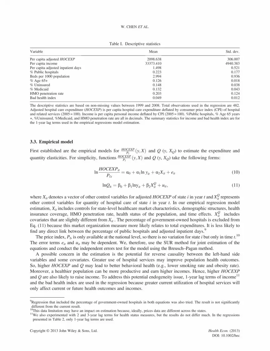
Table I. Descriptive statistics
Variable Mean Std. dev.
Per capita adjusted HOCEXP 2098.638 306.007Per capita income 33373.410 4940.383Per capita adjusted inpatient days 1.498 0.521% Public hospitals 0.223 0.177Beds per 1000 population 2.994 0.936% Age 65+ 0.126 0.018% Uninsured 0.148 0.038% Medicaid 0.132 0.043HMO penetration rate 0.203 0.124Bad health index 0.049 0.012
The descriptive statistics are based on non-missing values between 1999 and 2008. Total observations used in the regression are 482.Adjusted hospital care expenditure (HOCEXP) is per capita hospital care expenditure deflated by consumer price index (CPI) of hospitaland related services (2005 = 100). Income is per capita personal income deflated by CPI (2005 = 100). %Public hospitals, % Age 65 years+, %Uninsured, %Medicaid, and HMO penetration rate are all in decimals. The summary statistics for income and bad health index are forthe 1-year lag terms used in the empirical regressions model estimation.
W. CHEN ET AL.
Copyright © 2013 John Wiley & Sons, Ltd. Health Econ. (2013)
DOI: 10.1002/hec
In order to obtain the income elasticity of HOCEXP and the quantity component elasticity, we need to
estimate Eqs. (10) and (11). Because the key variables are already in the log form, the coefficient of income
in each equation gives the elasticity directly. According to Eq. (9) in our theoretical model, the quality elasticity
can then be derived by subtracting the quantity elasticity from the income elasticity.
4. EMPIRICAL ESTIMATION RESULTS
4.1. Model estimation
The SUR method is applied to jointly estimate both equations. SUR generates more efficient parameter
estimates compared with OLS under the assumption of cross-equation error correlation. This assumption is then
tested by the Breusch–Pagan test of independence (see, bottom of the regression results in Table II). The SUR
estimation is performed in STATA 11 (College Station, TX, USA) with the iteration option.12 Under the SUR,
the iteration converges to the maximum likelihood results. These are reported in Table II.
In both equations, we control for the time effect by including a time trend.13 According to the regression
results of Eq. (1), the highly statistically significant and positive income coefficient estimate indicates the
income elasticity to be 0.427 (std. error = 0.044, implications are discussed in more detail in Section 4.2).
The share of public hospitals tends to be negatively associated with adjusted HOCEXP. The effect of
hospital capacity, measured by hospital beds, is positive and significant, which could imply the presence
of induced demand.
The percentage of the population age 65 years and older also has the expected positive sign. As it is
commonly observed that healthcare spending during the last few years of life accounts for a large share of
the total healthcare spending in one’s entire life, it naturally follows that states with greater proportion of the
elderly residents tend to have higher HOCEXP.14 The proportion of the population without insurance is
negatively related to HOCEXP, whereas the percentage of Medicaid enrollees has a positive effect. Uninsured
individuals are likely to limit their own health services use in order to avoid medical costs. Medicaid enrollees,
on the other hand, tend to suffer from the moral hazard problem in which more health service use is encouraged
given the low cost. The coefficient of the HMO penetration rate shows the cost-saving effect of managed care.
The bad health index is positively associated with HOCEXP, which means higher obesity rates or smoking
rates increase HOCEXP, which is as expected. The estimated parameter of the time trend is negative.
The estimation results for Eq. (2) show an income coefficient not significantly different from zero,
suggesting that hospital care quantity is inelastic to an income change (Section 4.2 discusses further the
quantity component elasticity). Similar to the results of Eq. (1), the number of hospital beds has a positive
and significant effect, the uninsured proportion and HMO penetration rate have negative and significant effects,
and the share of Medicaid enrollees has a positive and significant effect on the quantity of hospital care used.
The elderly population share is not significant in Eq. (2). The bad health index has a surprisingly negative sign,
12It iterates over the estimated disturbance covariance matrix and parameter estimates until the parameter estimates converge.13Regression experiments without the time trend or with an additional time trend square term were also run. The log-likelihood ratio testresults suggest preference for the model with the time trend included. The time trend square, however, is not significant and thereforeexcluded from the regression. Moreover, an earlier version of this paper used state fixed effects and year fixed effects in each equation.They tend to pick up much of the explanatory power of income differences across states. Using state and year fixed effects in the currentmodel generates income elasticities that are not statistically different from zero. This evidence is consistent with those in earlier research.For example, Acemoglu et al. (2012) have some of their OLS income elasticity estimates close to zero but statistically insignificant whenincluding state fixed effects. They suspect it is due to the endogeneity problem between income and expenditures leading to biased OLSestimates. In our case, one potential explanation could be that using the 1-year lag of income could not fully control for the possibleendogeneity problem. Although finding a plausible instrumental variable for income may improve the estimation result, it is not an easyfeat to accomplish in addition to our primary goal in this paper. Therefore, it may be one limitation of our paper that is admittedly commonto many empirical econometric models.
14As in the work of Shang and Goldman (2008), we also experimented with ‘life expectancy’. While the resulting estimates of the incomeelasticity of HOCEXP are similar, the model with the population aging factor and bad health index fares slightly better.
QUALITY–QUANTITY DECOMPOSITION OF INCOME ELASTICITY OF HOSPITAL CARE
Copyright © 2013 John Wiley & Sons, Ltd. Health Econ. (2013)
DOI: 10.1002/hec

meaning more obese individuals and smokers are associated with fewer inpatient days. This may be because
obesity and smoking are chronic conditions that do not require acute and intensive hospital care. The time trend
is positive in Eq. (2).
The adjusted R2 values are 0.565 for the first equation and 0.881 for the second equation. The χ2 statistics
(617 and 3564 for two equations, respectively) indicate the regressions to be jointly significant. The
Breusch–Pagan test is also conducted to test the independence of the two equations. The correlation coefficient
of the residuals from the two jointly estimated equations is 0.566. The corresponding χ2 statistics (with p = 0)
suggests rejecting the independence of errors hypothesis.
4.2. Estimates of income elasticity and its quantity and quality components
As the SUR system estimates of Eq. (1) indicate in Table II, the highly significant income elasticity of adjusted
HOCEXP (0.427) implies that a 10% rise in real per capita income would tend to increase adjusted HOCEXP
by 4.27%. Moreover, Eq. (2) implies the estimated quantity elasticity to be insignificantly different from zero. It
suggests that the quantity of hospital care responds little to income changes. This may not be so surprising for
several reasons: (i) US hospital care is provided regardless of the ability to pay; (ii) demand for hospital care is
based more on medical needs and thus less likely to increase with income; and (iii) patients cannot choose their
quantity of hospital care freely as consumers do in other markets.
Table II. Seemingly unrelated regressions (SUR) model estimates
Coef. Std. err. Adj. R2
χ2
Equation 1log of adjusted HOCEXP 0.565 617.06log of income t� 1 0.427
***0.044
% public hospitals �0.048*
0.025log of beds 0.250
***0.022
% 65 years + 1.451***
0.349% uninsured �0.781
***0.134
% Medicaid 0.852***
0.118HMO rate �0.195
***0.053
Bad health index t� 1 1.101**
0.479Time trend �0.006
***0.002
Constant 2.770***
0.465
Equation 2log of adjusted inpatient days 0.881 3564.47log of income t� 1 0.035 0.050log of beds 0.997
***0.025
% 65 years + �0.099 0.384% uninsured �1.406
***0.152
% Medicaid 0.344**
0.135HMO rate �0.274
***0.059
Bad health indext� 1 �3.008***
0.546Time trend 0.025
***0.002
Constant �0.831 0.528
Derived quality elasticity 0.391***
0.044Correlation coef. of residuals 0.566Breusch–Pagan test χ
2= 154 (Pr. = 0)
Complete descriptions of the variables in this model are given in Table I.Statistical significance level:
*:10%,
**: 5%,
***:1%.
Number of observations in both equations is 482.The calculated standard error of derived quality elasticity is 0.044.The two equations are jointly estimated using SUR. The correlation coefficient of residuals and Breusch–Pagan test of independenceconfirms the dependence of the two equations.
W. CHEN ET AL.
Copyright © 2013 John Wiley & Sons, Ltd. Health Econ. (2013)
DOI: 10.1002/hec
The implied (Eq. (9)) estimate of the quality elasticity component of the income elasticity of HOCEXP is
0.391 (calculated std. error = 0.04415). Because the numerically small but positive quantity elasticity
component is not significant, almost all of the income elasticity derives from the quality component.
Altogether, the results suggest that income has little effect on the quantity of hospital care. Most of the effect
of income on HOCEXP is through quality changes in our model.
5. SUMMARY DISCUSSION AND IMPLICATIONS
For the first time in this line of work, we decompose the US income elasticity of HOCEXP into its quantity and
quality components with the goal of providing estimates for benchmarking the implications for hospital cost
containment policies in the context of the expansion of hospital care coverage following the full implementation
of the 2010 US healthcare law.
Using 1999–2008 US state-level panel data, we estimate the relationships among adjusted hospital care
expenditure, quantity of care measured, and real income using the SUR method. Given the controversy on var-
ious quality measures for hospital care, we model it in a way that requires no explicit specification of a quality
measure. Instead, income and quantity elasticities are first estimated, and the quality elasticity is then derived as
the difference between the two. Pure price effect is also controlled for in the model by introducing the price index
of a fixed basket of hospital services, measured by the consumer price index in hospital and related services.
The estimated income elasticity in our study is approximately 0.427. There are extremely few past studies
focusing on the hospital expenditure sub-category (HOCEXP) of the total healthcare spending (HEXP) for
comparison, and none focused on decomposing the income elasticity into its quality and quantity components.
One recent study on the determinants of US HOCEXP (Acemoglu et al., 2012) estimated the income elasticity
to be 0.568 (std. error = 0.263) on the basis of the use of state-year observations for the entire US geographic
sample. Despite the differences in the methodological approaches of the study of Acemoglu et al. (1970–1990,
US state-level data) and our investigation (1999–2008, US state-level panel data), the numerical magnitude of
the difference in the estimated income elasticities of HOCEXP is quite small. As earlier discussed in this paper,
modeling with a longer data span (e.g., as in the work of Acemoglu et al., 2012) would tend to yield a higher
income elasticity estimate.
Comparing our study’s income elasticity of HOCEXP with those of past studies on total HEXP using aggre-
gated data stimulates interesting discussions as well, past study estimates range widely from ≅ 0 to significantly
greater than 1. Costa-Font et al. (2011) use a meta-regression analysis to control for publication selection and
aggregation bias and find the corrected estimates to range from 0.4 to 0.8. Our estimate, based on modeling the
HOCEXP sub-category data, falling in the lower portion of this bound suggests that hospital care is both a
normal good and more of a stronger necessity than aggregated healthcare (HEXP) as a commodity. In effect,
hospital care confers significant physiological benefits.
Our study findings reveal that a large and significant share of the rise in HOCEXP has more to do with
quality than quantity of care purchased as income grows. Caution, however, that healthcare ‘ … quality is a
multi-dimensional concept that incorporates the ability, effort, and time that physicians spend in making a
diagnosis and providing treatment, as well as various attributes of the delivery of health services, such as
attentiveness, care, and diligence’ (Sloan and Hsieh, 2012, p. 279). Moreover, technological sophistication is
a core distinguishing attribute of hospitals (ibid, p. 220). Therefore, as heterogeneities characterize hospital care
quality and their technological imperatives, it is conceptually challenging to disentangle and isolate their
effects. Notably, the 0.391 implied quality portion of the estimated income elasticity of HOCEXP model here
mimics the 0.323 upper bound estimate of the contribution of technological progress to the rise in US
healthcare costs reported by Abrantes-Metz (2012).
15Given θ = ε� η in Eq. (9), the standard error of the quality elasticity is derived on the basis of Var(θ) =Var(ε)� 2Cov(ε,η) +Var(η). Cov(ε,η) is obtained through post-estimation command ‘matrix list e(V)’.
QUALITY–QUANTITY DECOMPOSITION OF INCOME ELASTICITY OF HOSPITAL CARE
Copyright © 2013 John Wiley & Sons, Ltd. Health Econ. (2013)
DOI: 10.1002/hec

One of the study policy implications is that as the economies of the US states grow, demand for higher
quality hospital care is expected to dominate the rise in the volume (or quantity) of care. As a consequence,
hospitals and their state regulators might consider optimal strategies that consistently target reimbursable
cost-containing quality improvements and implement incentives leading to more efficient production of
services as the quantity of hospital care demanded (volume) is poised to also grow with the full implementation
mandates of the 2010 Affordable Care Act.
CONFLICT OF INTEREST
The authors have no conflict of interest.
ACKNOWLEDGEMENTS
An earlier version of this work was presented at the 2012 biennial meetings of The American Society of Health
Economists (ASHEcon), University of Minnesota, Minneapolis, MN, USA. We thank Frank Lichtenberg and
the conference participants for their helpful comments on earlier drafts of this work. We also thank the journal
editors and two anonymous referees whose constructive suggestions have raised the quality outcome of this
research. The standard disclaimer applies, however.
REFERENCES
Abrantes-Metz RM. 2012. The contribution of innovation to health care costs: at least 50%? Social Science Research Networkworking papers series, August, 2012. Available from: http://dx.doi.org/10.2139/ssrn2121688 [accessed Sept. 2012].
Acemoglu D, Finkelstein A, Notowidigdo MJ. 2012. Income and health spending: evidence from oil price shocks. Reviewof Economics and Statistics, DOI: 10.1162/REST_a_00306
Aizcorbe A, Nestoriak N. 2011. Changing mix of medical care services: stylized facts and implications for price indexes.Journal of Health Economics 30(3): 568–74.
Akin J, Guilkey D, Denton E. 1995. Quality of services and demand for healthcare in Nigeria: a multinomial Probitestimation. Social Science and Medicine 40: 1527–1537.
Archibald R, Gillingham R. 1981. A decomposition of the price and income elasticities of the consumer demand forgasoline. Southern Economic Journal 47(4): 1021–1031.
Bils M, Klenow PJ. 2001. Quantifying quality growth. American Economic Review 91(4): 1006–1030.Bradley TB, Kominski GF. 1992. Contributions of case mix and intensity change to hospital cost increases. Healthcare
Financing Review 14(2): 151–63.Bundorf MK, Royalty A, BakerL C. 2009. Healthcare cost growth among the privately insured.Health Affairs 28(5): 1294–1304.Chernew M, Newhouse JP. 2012. Healthcare spending growth, Chapter 1. In Handbook of Health Economics, Pauly MV,
McGuire TG, Barros PP (eds). Elsevier B.V.Copnell B, Hagger V, Wilson SG, Evans SM, Sprivulis PC, Cameron PA. 2009. Measuring the quality of hospital care: an
inventory of indicators. Internal Medicine Journal 39: 352–360.Costa-Font J, Gemmill M, Rubert G. 2011. Biases in the healthcare luxury good hypothesis: a meta-regression analysis.
Journal of the Royal Statistical Society: Series A (Statistics in Society) 174(1): 95–107.Cuckler G, Martin A, Whittle L, Heffler S, Sisko A, Lassman D, Benson J. 2011. Health spending by state of residence,
1991–2009. Medicare Medicaid Research Review 1(4): E1–E30.Deaton A. 1988. Quality, quantity, and spatial variation of price. American Economic Review 78(3): 418–430.Di Matteo L. 2003.The income elasticity of healthcare spending: a comparison of parametric and nonparametric approaches.
European Journal of Health Economics 4(1): 20–29.Finkelstein EA, Trogdon JG, Cohen JW, Dietz W. 2009. Annual medical spending attributable to obesity: payer- and
service-specific estimates. Health Affairs 28(5): w822–w831.Gale F, Huang K. 2007. Demand for food quantity and quality in China. Economic Research Report No. (ERR-32) 40.Gertler PJ. 1985. A decomposition of the elasticity of medicaid nursing home expenditures into price, quality, and quantity
effects. NBER Working Paper No. 1751.
W. CHEN ET AL.
Copyright © 2013 John Wiley & Sons, Ltd. Health Econ. (2013)
DOI: 10.1002/hec
Getzen TE. 2000. Healthcare is an individual necessity and a national luxury: applying multilevel decision models to theanalysis of healthcare expenditures. Journal of Health Economics 19(2): 259–270.
Glenn B. 2013. Family practices are No. 1 target for hospital acquisitions. Medical Economics. Available from: http://medicaleconomics.modernmedicine.com/medical-economics/news/user-defined-tags/acquisitions/family-practices-are-no-1-target-hospital-acqu [Accessed: March 29, 2013].
Grabowski D. 2001. Does an increase in the medicaid reimbursement rate improve bursing home quality? Journal ofGerontology: Social Sciences 56B(2): S84–S93.
Hicks WW, Johnson SR. 1968. Quantity and quality components for income elasticities of demand for food. AmericanJournal of Agricultural Economics 50(5): 1512–1517.
Jappelli T, Pistaferri L, Weber G. 2007. Healthcare quality, economic inequality, and precautionary saving. Health Economics16(4): 327–346.
Lichtenberg FR. 2011. The quality of medical care, behavioral risk factors, and longevity growth. International Journal ofHealthcare Finance and Economics 11: 1–34.
Martin AB, Lassman D, Washington B, Catlin A, The National Health Expenditure Accounts Team. 2012. Growth in UShealth spending remained slow in 2010; health share of gross domestic product was unchanged from 2009. HealthAffairs 31: 208–219.
Newhouse JP. 1970. Toward a theory of nonprofit institutions: an economic model of a hospital. American EconomicReview 60(1): 64–74.
Newhouse JP. 1977. Medical care expenditure: a cross-national survey. Journal of Human Resources 12: 115–125.Newhouse JP. 1992. Medical care costs: how much welfare loss? Journal of Economic Perspectives 6(3): 3–21.Newhouse JP, Phelps CE. 1976. New estimates of price and income elasticities of medical care services. In The Role of
Health Insurance in the Health Services Sector. National Bureau of Economic Research, Inc: Cambridge, MA; 261–320.Okunade AA, Murthy VNR. 2002. Technology as a “major driver” of healthcare costs: a cointegration analysis of the
Newhouse conjecture. Journal of Health Economics 21(1): 147–159.Paluch M, Kneip A, Hildenbrand W. 2012. Individual versus aggregate income elasticities for heterogeneous populations.
Journal of Applied Econometrics 27(5): 847–869.Peden EA, Freeland MS. 1998. Insurance effects on US medical spending. Health Economics 7: 671–687.Ringel JS, Hosek SD, Vollaard BA,Mahnovski S. 2002. The elasticity of demand for healthcare. RAND report MR-1355-OSD.Schneider H. 2008. Incorporating healthcare quality into health antitrust law. BMC Health Services Research 8: 89.Schwartz WB. 1987. The inevitable failure of current cost-containment strategies. Journal of the American Medical
Association 257(2): 220–224.Shang B, Goldman D. 2008. Does age or life expectancy better predict health care expenditures? Health Economics 17:
487–501.Sloan FA, Hsieh CR. 2012. Quality of care and medical malpractice. In Health Economics. MIT Press: Cambridge, MA;
275–317.Smith S, Newhouse JP, Freeland MS. 2009. Income, insurance, and technology: why does health spending outpace
economic growth? Health Affairs 28(5): 1276–1284.
QUALITY–QUANTITY DECOMPOSITION OF INCOME ELASTICITY OF HOSPITAL CARE
Copyright © 2013 John Wiley & Sons, Ltd. Health Econ. (2013)
DOI: 10.1002/hec