Louisiana State UniversityLSU Digital Commons
LSU Doctoral Dissertations Graduate School
2017
Protection Challenges of Distributed EnergyResources Integration In Power SystemsPooria MohammadiLouisiana State University and Agricultural and Mechanical College, [email protected]
Follow this and additional works at: https://digitalcommons.lsu.edu/gradschool_dissertations
Part of the Electrical and Computer Engineering Commons
This Dissertation is brought to you for free and open access by the Graduate School at LSU Digital Commons. It has been accepted for inclusion inLSU Doctoral Dissertations by an authorized graduate school editor of LSU Digital Commons. For more information, please [email protected].
Recommended CitationMohammadi, Pooria, "Protection Challenges of Distributed Energy Resources Integration In Power Systems" (2017). LSU DoctoralDissertations. 4340.https://digitalcommons.lsu.edu/gradschool_dissertations/4340

PROTECTION CHALLENGES OF DISTRIBUTED ENERGY RESOURCES
INTEGRATION IN POWER SYSTEMS
A Dissertation
Submitted to the Graduate Faculty of the
Louisiana State University and
Agricultural and Mechanical College
in partial fulfillment of the
requirements for the degree of
Doctor of Philosophy
in
The School of Electrical Engineering and Computer Science
by
Pooria Mohammadi
B.S., Iran University of science and Technology, 2005
M.S., University of Texas at Tyler, 2013
August 2017

ii
Dedicated to my parents.

iii
Acknowledgements
First I would like to acknowledge my advisor Dr. Shahab Mehraeen for his support, excellent
guidance, and ultimate mentorship over the years. Without his insightful and innovative ideas, this
thesis could not have been accomplished.
Special thanks goes to my family of whom I received invaluable support and constant
dedication. I want to thank to all my friends and also colleagues at Louisiana State University
Smart Grid and Renewable Power Laboratory: Control and Protection for their helps and
supports.
I would like to thank LSU faculty members Leszek S Czarnecki, Hsiao-Chun Wu, Mehdi
Zeidouni, Mehdi Farasat, and Amin Kargarian Marvasti for being members of my general and oral
examination committees and providing me with their thoughtful comments and suggestions.
I also express my appreciation to the Entergy Services and specifically to Tom Field and Mark
Bruckner from Transmission Design Basis group for their support and encouragement throughout
this work.
I also thank the administrative team at the Division of Electrical and Computer Engineering,
Louisiana State University. I wish to express my appreciation to Beth R. Cochran for her constant
support.
iv
TABLE OF CONTENTS Acknowledgements .................................................................................................................. iii
Abstract ........................................................................................................................................ vi
Chapter 1. Introduction ............................................................................................................. 8 1.1. Background and Motivation ........................................................................................... 8 1.2. Outline of the Dissertation ............................................................................................ 14
Chapter 2. Power System PMU Placement for Fault Observability and Location .. 16 2.1. Introduction ................................................................................................................... 16 2.2. Sensitivity Analysis ...................................................................................................... 20
2.2.1. Voltage Sensitivity Indices ................................................................................. 23 2.2.2. Current Sensitivity Indices ................................................................................. 24
2.3. Sensitivity Analysis Criteria for OPP for Fault Location and Observability ................ 27 2.3.1. Sensitivity Requirements .................................................................................... 27 2.3.2. Uniqueness and Multi Estimation ...................................................................... 30
2.4. Proposed Algorithm for OPP and Artificial Neural Network Fault Locator ................ 31 2.5. An Example using IEEE 7-Bus Case ............................................................................ 35 2.6. Artificial Neural Network (ANN) Fault Locator .......................................................... 40 2.7. Proposed Algorithm Results and Discussion ................................................................ 42 2.8. Conclusion .................................................................................................................... 46 2.9. References ..................................................................................................................... 47
Chapter 3. Overhead Radial Distribution Networks ....................................................... 50 3.1. Introduction ................................................................................................................... 50 3.2. 13-Bus network ............................................................................................................. 50 3.3. Network’s Voltages ...................................................................................................... 52 3.4. Solar Radiation Change ................................................................................................ 52 3.5. Cloud Effects ................................................................................................................ 54
3.5.1. Small Cloud ........................................................................................................ 57 3.5.2. Scattered Cloud .................................................................................................. 58 3.5.3. Large Cloud........................................................................................................ 60
3.6. Reactive Power Compensation ..................................................................................... 63 3.6.1. Scenario 1: Connected Mode ............................................................................. 63 3.6.2. Scenario 2: Islanded Mode ................................................................................ 65
3.7. Fault Current Level ....................................................................................................... 68 3.8. Harmonic Analysis........................................................................................................ 71
3.8.1. Effect of PV Penetration Level ........................................................................... 72 3.8.2. Effect of Capacitor Bank .................................................................................... 73 3.8.3. Effect of Bus Location ........................................................................................ 74 3.8.4. Effect of Load Level............................................................................................ 75
3.9. Standards Regulations for Harmonic ............................................................................ 76 3.10.Filtering effect on Harmonic ......................................................................................... 78 3.11.Smart Inverter and Battery Storage............................................................................... 80
3.11.1.Smart Inverter Effects ........................................................................................ 80
v
3.11.2.Battery Storage .................................................................................................. 82 3.12.References ..................................................................................................................... 83
Chapter 4. Challenges of PV Integration in Low-Voltage Secondary (Downtown)
Networks .................................................................................................................................... 85 4.1. Introduction ................................................................................................................... 85 4.2. Low-Voltage Secondary Network ................................................................................ 88
4.2.1. Network under Study .......................................................................................... 88 4.2.2. Network Model ................................................................................................... 91 4.2.3. Microprocessor Network Protector Relay (MNPR) ........................................... 92 4.2.4. Smart Network Protector Relay (SNPR) ............................................................ 94
4.3. MNPR Operation .......................................................................................................... 97 4.3.1. PV Arrangements ............................................................................................... 98 4.3.2. MNPR Trip Statistics .......................................................................................... 99 4.3.3. Distribution Line Overload Statistics ............................................................... 104 4.3.4. MNPR Reclose operation ................................................................................. 105
4.4. Case Studies for SNPR ............................................................................................... 106 4.5. Cloud Effect ................................................................................................................ 108 4.6. Voltage Profile ............................................................................................................ 111 4.7. A Random PV Allocation Approach Simulation ........................................................ 112 4.8. Communication Requirements for Smart Network Protector (SNPR) ....................... 117
4.8.1. Smart Network Protector Relay (SNPR) .......................................................... 118 4.8.2. Communication ................................................................................................ 119 4.8.3. Industrial Communication Protocols ............................................................... 120
4.9. Conclusion .................................................................................................................. 123 4.10.References ................................................................................................................... 124
Chapter 5. Conclusive Remarks and Future Works ...................................................... 126 5.1. Conclusion .................................................................................................................. 126 5.2. Future Works .............................................................................................................. 128
Appendix .................................................................................................................................. 129
Vita... ......................................................................................................................................... 129

vi
Abstract
It is a century that electrical power system are the main source of energy for the societies and
industries. Most parts of these infrastructures are built long time ago. There are plenty of high
rating high voltage equipment which are designed and manufactured in mid-20th and are currently
operating in United States’ power network. These assets are capable to do what they are doing
now. However, the issue rises with the recent trend, i.e. DERs integration, causing fundamental
changes in electrical power systems and violating traditional network design basis in various ways.
Recently, there have been a steep rise in demands for Distributed Energy Resources (DERs)
integration. There are various incentives for demand in such integrations and employment of
distributed and renewable energy resources. However, it violates the most fundamental assumption
in power system traditional designs. That is the power flows from the generation (upstream) toward
the load locations (downstream). Currently operating power systems are designed based on this
assumption and consequently their equipment ratings, operational details, protection schemes, and
protections settings. Violating these designs and operational settings leads toward reducing the
power reliability and increasing outages, which are opposite of the DERs integration goals.
The DERs integration and its consequences happen in both transmission and distribution
levels. Both of these networks effects of DERs integration are discussed in this dissertation. The
transmission level issues are explained in brief and more analytical approach while the
transmission network challenges are provided in details using both field data and simulation
results. It is worth mentioning that DERs integration is aligned with the goal to lead toward a smart
grid. This can be considered the most fundamental network reconfiguration that has ever
experienced and requires various preparations. Both long term and short term solutions are

vii
proposed for the explained challenges and corresponding results are provided to illustrate the
effectiveness of the proposed solutions. The author believes that developing and considering short
term solutions can make the transition period toward reaching the smart grid possible. Meanwhile,
long term approaches should also be planned for the final smart grid development and operation
details.

8
Chapter 1
Introduction
1.1. Background and Motivation
The integration of Distributed Energy Resources (DERs) into the power grids has brought
many new challenges to the currently operating power system and networks. There are various
incentives for this integration convincing governments to promote it by various means as well as
attracting the customers. The DERs integration, where mostly renewable energy resources are used
as the base energy sources for them, can bring benefits such as reducing fossil fuels consumption
and dependability, reducing Carbone dioxide, increasing system reliability, increasing profitability
and customer owned generation, decreasing generation unit’s capital investment, islanding
operation, etc. It is obvious that the electric network safe operation and power reliability is the
most important aspect which shouldn’t have an adverse effect by this integration. However, the
DERs integration makes significant change in the network fundamentals in a way that can be
considered as a reconfiguration aligned toward establishing a smart grid.
Currently operating power systems are designed and operating based on a fundamental
assumption which is unidirectional power flow. Integrating DERs and allowing loads (customers)
to generate power and possibly even export at some period of times causes important changes in
the network operation. When all DERs power generation are less than their local assumption, i.e.
no power is being exported, the network operating point is significantly different than what it is
designed for. This can critically affect the protection schemes, protective devices, and equipment
ratings. Various DER generating units can easily have different fault current contribution
comparing to what the system is designed for. On the other hand, the unidirectional power flow
9
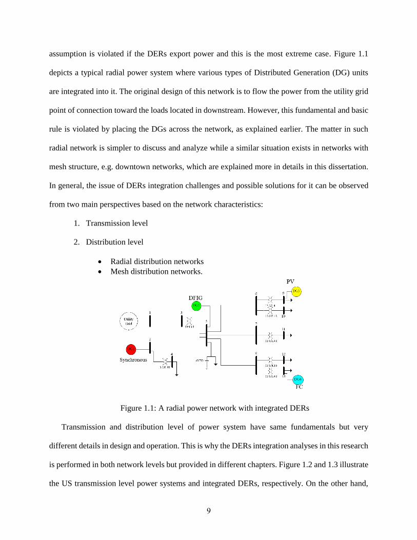
assumption is violated if the DERs export power and this is the most extreme case. Figure 1.1
depicts a typical radial power system where various types of Distributed Generation (DG) units
are integrated into it. The original design of this network is to flow the power from the utility grid
point of connection toward the loads located in downstream. However, this fundamental and basic
rule is violated by placing the DGs across the network, as explained earlier. The matter in such
radial network is simpler to discuss and analyze while a similar situation exists in networks with
mesh structure, e.g. downtown networks, which are explained more in details in this dissertation.
In general, the issue of DERs integration challenges and possible solutions for it can be observed
from two main perspectives based on the network characteristics:
1. Transmission level
2. Distribution level
Radial distribution networks
Mesh distribution networks.
Figure 1.1: A radial power network with integrated DERs
Transmission and distribution level of power system have same fundamentals but very
different details in design and operation. This is why the DERs integration analyses in this research
is performed in both network levels but provided in different chapters. Figure 1.2 and 1.3 illustrate
the US transmission level power systems and integrated DERs, respectively. On the other hand,

10
distribution networks can be in radial and mesh structures. The author has investigated and
considered the radial distribution networks impacts from DGs integration during his master degree.
Hence, radial distribution network analyses and results here are limited to the field experiences
and valuable outcomes. But distribution networks in mesh configuration are paid extra attention
in this dissertation. A good example for this networks is low-voltage secondary networks which
are also called downtown networks. Because of the high important of the power reliability and
quality in such networks and also the customer importance in such regions, the DERs integration
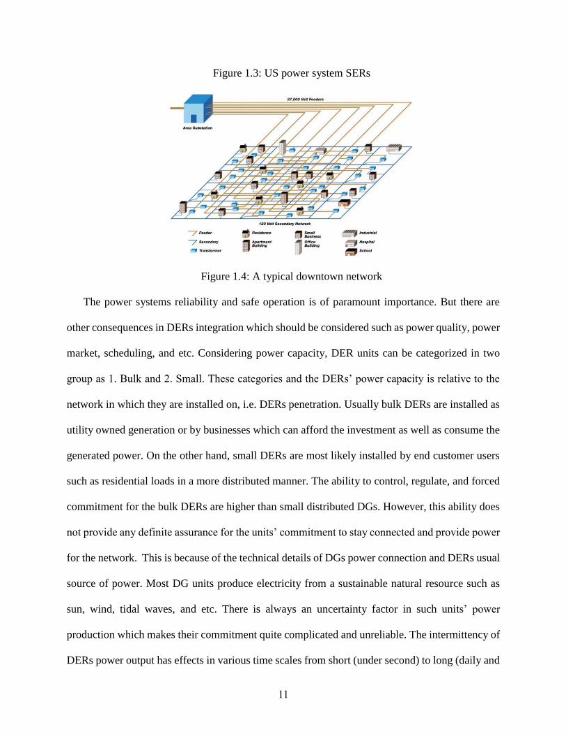
is a critical issue to be analyzed there. Figure 1.4 depicts a typical downtown network where DGs
can be installed at customer locations.
Figure 1.2: US power system transmission lines
11
Figure 1.3: US power system SERs
Figure 1.4: A typical downtown network
The power systems reliability and safe operation is of paramount importance. But there are
other consequences in DERs integration which should be considered such as power quality, power
market, scheduling, and etc. Considering power capacity, DER units can be categorized in two
group as 1. Bulk and 2. Small. These categories and the DERs’ power capacity is relative to the
network in which they are installed on, i.e. DERs penetration. Usually bulk DERs are installed as
utility owned generation or by businesses which can afford the investment as well as consume the
generated power. On the other hand, small DERs are most likely installed by end customer users
such as residential loads in a more distributed manner. The ability to control, regulate, and forced
commitment for the bulk DERs are higher than small distributed DGs. However, this ability does
not provide any definite assurance for the units’ commitment to stay connected and provide power
for the network. This is because of the technical details of DGs power connection and DERs usual
source of power. Most DG units produce electricity from a sustainable natural resource such as
sun, wind, tidal waves, and etc. There is always an uncertainty factor in such units’ power
production which makes their commitment quite complicated and unreliable. The intermittency of
DERs power output has effects in various time scales from short (under second) to long (daily and

12
more than monthly). For instance, Photovoltaic (PV) cell performance is dependent on the
intermittent solar radiation causing power variations and voltage fluctuations. In general, this
raises concerns about networks voltage stability and power quality which are addressed in this
dissertation. However this power output unpredictability causes uncertainties in long term power
generation scheduled commitments. It should be mentioned that the explained issue is also
applicable to the DGs which their source of energy is not an intermittent natural resource but rather
is sources such as fuel cell, diesel, etc. Fuel availability, customer willingness, market price, and
connection details can still affect such units’ commitment in an unpredictable way. Basically,
DERs unit power production and network commitment depend on three main factors:
1. Energy source availability,
2. Owner will,
3. Operation and connection technical details.
Majority of DG units require an electric power conversion unit at their connection point to the
network. This is either because of stabilizing the output ripples due to the energy source changes
(wind, solar) or forming the electricity to the operating frequency and form. This is mostly
performed by power electronic device where their control algorithm is complicated topic beyond
of this context topic. Power electronic converters and inverters are widely used for power
conversion and control proposes in most of DGs. A good example for this are PV units. Most PVs
are connecting to the grid by an inverter unit converting dc to ac and some are equipped with
battery storage systems for better performance and reliability. As integration of PV units are
becoming more prevalent in distribution networks, they are more likely to be an important active
element of such networks and will have significant impacts on the power reliability and quality.
With recent industry progresses, both small residential and larger units’ inverters are enabled with
13
control and strategic functions to improve their functionality. Also, newer inverter units take
advantage of communication systems. That is, PV units can comply with the utility regulations
either autonomously, via fixed and variable set points, or controlled through communication
infrastructures. One of the most well-known equipment with these capabilities are smart inverters.
Autonomous control and standalone functionality are sued in the last decade. Where these control
methods are useful for islanding scenarios they are not neither completely safe, in terms of
operation and cross effects, nor optimized. By making communication infrastructures more
available such control strategies are tend to be more optimized and unified in following their goals.
These objectives can voltage control, reactive power compensation, active power control, peak
shaving, time shifting, and even dynamic variables control such as frequency. There are multiple
schemes to collect the data and information from DER units and transfer them to a central operation
unit to send out commands on how to react in a specific time or to a specific phenomenon. This
way the DERs capabilities and smart inverters functionalities are closer to be fully deployed. Such
schemes which can be considered a collection of DERs capability, smart inverter functionality,
communication infrastructures, fast system solvers and analyzers, and optimization algorithms can
be found in applications such as Energy Management Systems (EMS) and Distribution
Management Systems (DMS). However, there are plenty of challenges in fully accomplished a
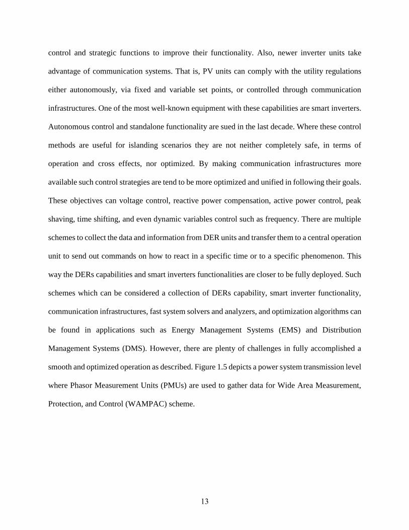
smooth and optimized operation as described. Figure 1.5 depicts a power system transmission level
where Phasor Measurement Units (PMUs) are used to gather data for Wide Area Measurement,
Protection, and Control (WAMPAC) scheme.
14
Figure 1.5: PMU equipped transmission power system for wide area protection
1.2. Outline of the Dissertation
The remainder of this dissertation is organized as follows. In Chapter 2, Phasor Measurement
Units (PMU) placement in transmission power system is discussed for system fault observability
and fault location. Measurements yielded from PMUs are GPS time stamped which makes them
capable for phasor estimation as well as frequency detection. This features along with high
resolution samples make PMU a key element to assist to solve the rising challenges of DERs
integration and system changes. Power system fault observability is achieved along with fault
detection when an optimized PMU placement algorithm is proposed. Extensive results and
discussions are provided in Chapter 2.
Chapter 3 presents results and studies for the DERs integration in overhead radial
distribution networks with extra attention to power quality concerns. DERs integration can cause
consequences regarding the voltage flicker, harmonics, etc. These are discussed and various IEEE
and ANSI standards are mentioned to compare the modelled network operation details with
allowed standard limits. It should be mentioned that PVs are widely used in this research as an
extreme case for power intermittency and due to high demand from their applications. PV units
are considered a good instance for DGs integration due to their smart inverter possible functions
DGs Operation Condition
PMU
PMU
PMU

15
effects and complexity and also feasibility for constructing a smart grid with required
communication infrastructure.
Chapter 4 discussed protection challenges for DERs and specifically PVs integration in low-
voltage secondary networks (downtown). Downtowns are one of the networks where there are high
demand for DERs integration and they are also vulnerable for such integration consequences. New
Orleans downtown network is modelled in this chapter and extensive analyses are performed
illustrating the protection scheme and elements malfunctioning leading toward network collapse.
It is shown that for a safe and reliable network operation the DERs penetration should be limited
to less than 16%. Another viable and economical solution is proposed in this chapter to resolve the
network protection issues when higher DERs penetration is allowed. Using the proposed method
more than 50% DER penetration can be integrated in the network. Penetrations higher than this
are discussed in Chapter 3 where other network specifications and ratings should be considered.
Chapter 5 summarizes the results and discussions in all chapter with concluding remarks.
Some discovered topis are also proposed here to be considered as possible future works aligned
with this line of research.
16
Chapter 2
Power System PMU Placement for Fault
Observability and Location
1.3. Introduction
The roles of synchronized Phasor Measurement Units (PMU) in power systems monitoring,
control, and protection are prominent and constantly developing [1]–[4]. The traditional
supervisory control and data acquisition (SCADA) systems collect data from the remote terminal
units (RTUs) that are mostly available in substations. With the global positioning system (GPS)
and by employing PMUs, accurate and time-synchronized measurement signals are now available.
This enables the operator to take advantage of wide area monitoring, protection and control
(WAMPAC) [5]. These applications include accurate fault location [6], normal and fault
observabilities [2], [7], and post-contingency analysis [8] as well as static analysis, identifying
system dynamics, transient stability prediction and control, voltage and frequency stability [8], etc.
PMU and WAMPAC should make it possible to safely operate smart grids employing the
maximum available capacity of renewable and distributed energy resources.
Pioneering studies on PMU introduction, development and utilization are performed by
Phadke et al. [1], [9]. In [1], the possibility of employing PMUs on all system buses is explored.
However, PMUs’ relatively high costs and their required infrastructure such as communication in
substations prevent the use of this solution. Therefore, many techniques and algorithms have been
proposed in recent years to find Optimal PMU Placement (OPP) in power systems targeting
system’s normal observability. This is done using algebraic and topological methods. System

17
normal observability is guaranteed using algebraic methods if the rank of the measurement matrix
is complete, i.e., it is equal to the number of system state variables. In topological methods, graph
theory is employed and normal observability is ensured if it is possible to have an observable
spanning tree [5]. These two approaches for OPP correspond to numerical observability and
topological observability, respectively [2], [10]. A power system is normally observable when all
of its bus voltage phasors are known using available measurements under normal operation [7].
The pioneering work in this topic is initially performed by [2] where an optimal set of PMUs are
achieved by a dual search algorithm using both modified bisecting search and simulated-
annealing-based method. Integer Linear Programming (ILP) is introduced in [3] considering
systems with and without zero injection buses (buses with no source or load). It is shown in [3]
that ILP is non-linear for cases with zero injection while it is linear in cases without zero injection.
ILP is later generalized in [11] addressing redundancy, partial observability and pre-existing
measurements. However, this method may result in local minima [12]. Limited PMU channels and
their failure is discussed in [5] using Binary Search. Approaches such as exhaustive search,
Genetic Algorithm, Tabu search, Greedy Algorithm, etc., are also discussed in the literature [13].
In addition, various cases of measurements such as direct PMU, conventional flow meters, zero
injection buses and pseudo-measurements are introduced in multiple literatures [13].
While many approaches are proposed to solve OPP problem for power system normal
observability (under normal operating condition), there are a very limited number of studies that
target OPP for fault observability. A power system is fault observable if voltage and current
phasors at both ends of all lines will be determinable during a fault scenario occurring at any point
of the system. It should be mentioned that normal observability does not guarantee fault

18
observability [7]. Thus, a normal observable power system may not be fully observable during
fault condition since fault alters the system structure.
Optimal PMU placement for fault observability is introduced by [14] and [15]. Authors in
[14] employ the popular one-bus-spaced strategy to find the OPP by Genetic Algorithm using only
PMU voltage measurements. The topic is expanded by [15] by considering zero injection buses
(that reduce the system size) using both PMU voltage and current measurements followed by ILP
methodology. In [7] weight vectors reflecting cost variables are considered for both PMU and
conventional flow measurements resulting in non-linear formulation in fault observability.
Optimal PMU placement for fault observability along with a fault location algorithm is utilized in
[14] and [16] when one-bus-spaced strategy is employed for simplicity.
Though the available approaches take advantage of various algorithms to impose
observability constraints, the important issue of measurement sensitivity (quality) and its impact
on OPP set and fault location is considered in very few literatures. Authors of [17] utilize a
minimization algorithm to reduce the number of sensors followed by considering the measurement
precision in the fault location problem [18] given the sensor locations; however, the precision has
not been used in the measurement optimal placement. The effect of the measurement precision in
PMU placement is of paramount importance and adds additional constraints to the available
methods while this has not been given enough attention in OPP solution methods. In addition, the
majority of past literature contemplates that the one-bus-spaced location strategy in PMU
placement is a necessary condition to attain fault location [16]; however, this chapter shows that
the set of critical measurement points to attain a desired accuracy in fault location, which is
typically smaller than that of the one-bus-spaced method, is more appropriate.

19
This research considers PMU direct measurements with adequate channel availability for
voltage and current measurements. A slightly different definition of fault observable system than
[7], [14]–[15] is adopted here. If location and impedance of all faults of interest in a power system
can be determined with predefined accuracy through a set of voltage and current measurements,
the system is considered fault observable. A unique function mapping between measurements and
faults is obtained and discussed in a systematic manner for the first time to the authors’ best
knowledge. The objectives of this research include:
1. Introduce sensitivity analysis in OPP problem for power systems fault observability. The
quality of measurements is assessed at PMU locations using the proposed sensitivity
indices. Thus, one can judge if a network bus is a good measurement location through
which faults can be located. Using the proposed sensitivity analysis, measurement
precision or inaccuracy instigated by the current transformers (CTs), potential transformers
(PTs), and PMUs can be incorporated in the OPP problem. Measurement quality is also
vital for other system analyses such as voltage stability, contingency studies, etc., which
are mostly fault related.
2. Formulate minimal PMU placement and find pertinent optimal PMU sets for fault
observability and fault location. That is, the proposed algorithm finds the optimal PMU
sets such that the faults are located uniquely, i.e. with no multi estimation, with desired
accuracy using minimum number of PMUs. Multi estimation is a condition where different
faults result in similar measurements in a selected PMU set.
3. Develop a fault locator by utilizing obtained optimal PMU set via artificial neural networks
(ANNs). The function approximation property of the ANNs is employed to map between
the faults and the measurements of the optimal PMU set.
20
Contingency as well as missing and additional measurements discussions are omitted due to
space limitation and cross-topic confusions. The remainder of this chapter is organized in the
following order: Section II presents the proposed sensitivity analysis and introduces the sensitivity
indices. In Section III, the sensitivity and multi estimation criteria are presented followed by the
proposed algorithm for solving OPP in Section IV. Section V includes simulation results of the
proposed method on the IEEE 7-bus, IEEE 14-bus, and IEEE 30-bus test systems followed by
artificial neural network fault locator results to test the proposed approach for fault location
application. Finally, concluding remarks are provided in Section VI.
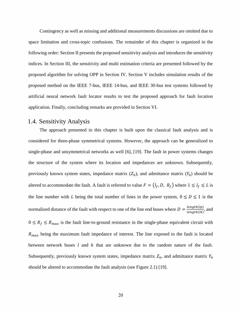
1.4. Sensitivity Analysis
The approach presented in this chapter is built upon the classical fault analysis and is
considered for three-phase symmetrical systems. However, the approach can be generalized to
single-phase and unsymmetrical networks as well [6], [19]. The fault in power systems changes
the structure of the system where its location and impedances are unknown. Subsequently,
previously known system states, impedance matrix (𝑍0), and admittance matrix (𝑌0) should be
altered to accommodate the fault. A fault is referred to value 𝐹 = (𝑙𝑓 , 𝐷, 𝑅𝑓) where 1 ≤ 𝑙𝑓 ≤ 𝐿 is
the line number with 𝐿 being the total number of lines in the power system, 0 ≤ 𝐷 ≤ 1 is the
normalized distance of the fault with respect to one of the line end buses where 𝐷 =𝑙𝑒𝑛𝑔𝑡ℎ(𝑙𝑝)
𝑙𝑒𝑛𝑔𝑡ℎ(𝑙𝑘), and
0 ≤ 𝑅𝑓 ≤ 𝑅𝑚𝑎𝑥 is the fault line-to-ground resistance in the single-phase equivalent circuit with
𝑅𝑚𝑎𝑥 being the maximum fault impedance of interest. The line exposed to the fault is located
between network buses 𝑙 and 𝑘 that are unknown due to the random nature of the fault.
Subsequently, previously known system states, impedance matrix 𝑍0, and admittance matrix 𝑌0
should be altered to accommodate the fault analysis (see Figure 2.1) [19].

21
𝑘 𝑙 𝑍𝑙𝑘
𝑍0 a) 𝑘 𝑙 𝑍𝑙𝑘 𝑍1 b)
𝑘 𝑙 𝑝 (1 − 𝐷) × 𝑍𝑙𝑘 𝑍2 c)
𝑘 𝑙 𝑝 (1 − 𝐷) × 𝑍𝑙𝑘 𝐷 × 𝑍𝑙𝑘 𝑍4
𝑅𝑓
e)
𝑍3 𝑘 𝑙 𝑝 (1 − 𝐷) × 𝑍𝑙𝑘 𝐷 × 𝑍𝑙𝑘 d)
Figure 2.1: Steps for Zbus modification: Z0 through Z3 are the steps of change in Zbus
This study considers faults on power system lines (note that faults on grid buses is a special
case). That is, an extra bus 𝑝 = 𝑁 + 1 is designated at the point of fault where 𝑁 is the network
total number of buses. Figure 1 shows the procedure of adding a fault to the system. The unfaulty
power system with known impedance matrix 𝑍0, voltages, and currents are depicted in Figure 2.1a.
Also, Figure 2.1d depicts the faulty system with the fault (on one of the network lines) and
impedance matrix 𝑍3 (fault not included). The line exposed to the fault is located between system
buses 𝑙 and 𝑘 that are unknown due to the random nature of the fault with unknown fault distance
𝐷 and fault resistance 𝑅𝑓.
Definitions: The following terms are frequently used in this chapter.
- Normal value: The value of a bus voltage or a line current in an unfaulty power system is called
normal value.
- Fault: A fault is referred to by value 𝐹 = (𝑙𝑓 , 𝐷, 𝑅𝑓) where 𝑙𝑓 ∈ 𝑳𝒇 = {1,2, … , 𝐿} is the line
number where fault occurs with 𝐿 being the total number of lines in the power system, 𝐷 ∈
𝐃 = [0,1] is the normalized distance of the fault with respect to one of the line end buses (𝐷 =
𝑙𝑒𝑛𝑔𝑡ℎ(𝑙𝑝)
𝑙𝑒𝑛𝑔𝑡ℎ(𝑙𝑘) from Fig. 1), and 𝑅𝑓 ∈ 𝐑𝒇 = [0, 𝑅𝑚𝑎𝑥] is the fault line-to-ground resistance in the
single-phase equivalent circuit with 𝑅𝑚𝑎𝑥 being the maximum fault resistance of interest. If

22
𝑅𝑚𝑎𝑥 is selected very small (short circuit), the loads can be ignored in the proposed method.
Otherwise, the load information may be needed to locate the fault accurately.
- Observant bus: Bus ℎ ∈ {1,2, … ,𝑁}, with 𝑁 being the total number of power system buses,
where a measurement device capable of measuring the bus voltage and currents (of the lines
connected to that bus) is installed, is an observant bus.
- Observant set: A set 𝐻 ⊆ {1,2, … ,𝑁} of observant buses is called an observant set.
- Adjacent bus: Bus 𝑢 is called an adjacent bus to observant bus ℎ if 𝑢 ∈ 𝑈ℎ with 𝑈ℎ is the set
of all connected buses to observant bus ℎ. Also, 𝑈ℎ is called adjacent set to observant bus ℎ
and has ℎ𝑐 many members; i.e., there are ℎ𝑐 many connected buses (lines) to observant bus ℎ.
- Multi estimation: Multi estimation is a condition where different faults cause similar measured
values in an observant set.
Four steps are required to modify 𝑍0 and obtain 𝑍4 (dashed elements in Fig. 1.b imply faulty
line removal from 𝑍𝑏𝑢𝑠):
Z1: Remove the transmission line between buses 𝑙 and 𝑘 by adding the line’s negative
impedance (−𝑍𝑙𝑘) between buses;
Z2: Add (1 − 𝐷) × 𝑍𝑙𝑘 between bus 𝑘 and new bus (𝑝);
Z3: Add 𝐷 × 𝑍𝑙𝑘 between bus 𝑙 and existing bus 𝑝;
Z4: Add 𝑅𝑓 between bus 𝑝 and ground reference node;
Each of these steps results in a new system with impedance matrix subscripted by the step
number as shown in Figure 2.1 [16]. By using the standard fault analysis, the voltage changes at
observant bus ℎ, (when fault 𝐹 occurs at bus 𝑝) can be described as
𝛥𝑉ℎ,𝐹 =𝑍3(ℎ,𝑝)
𝑍3(𝑝,𝑝)+𝑅𝑓× 𝑉𝑝𝑟𝑒𝑓 (1)

23
where 𝑍3(ℎ, 𝑝) is the (ℎ, 𝑝) entree of Z3, 𝑍3(𝑝, 𝑝) is the system Thevenin impedance seen
from imaginary bus 𝑝 , and 𝑉𝑝𝑟𝑒𝑓 is the prefault voltage at the point of fault in the system. With
the assumption of linear voltage drop along the transmission lines between buses and by ignoring
line capacitances to avoid complexity, 𝑉𝑝𝑟𝑒𝑓 can be calculated as:
𝑉𝑝𝑟𝑒𝑓 = 𝑉𝑙 + (1 − 𝐷) × (𝑉𝑙 − 𝑉𝑘). (2)
For more accurate calculation in long transmission lines, hyperbolic voltage drop can be
considered [16]. From the previous discussion, voltage and current rates of change in all buses of
the system can be calculated by using original impedance matrix Z0 along with 𝐷 and 𝑅𝑓, as will
be explained next.
1.4.1. Voltage Sensitivity Indices
Voltage change in observant bus ℎ due to fault 𝐹 = (𝑙𝑓 , 𝐷, 𝑅𝑓) is presented in (1). Using
the chain rule on 𝛥𝑉ℎ, voltage sensitivity indices are defined as derivatives of 𝐷 and 𝑅𝑓 with respect
to 𝛥𝑉ℎ as
𝑆ℎ,𝐹𝐷𝑉 = (
𝜕𝛥𝑉ℎ
𝜕𝐷)−1
=𝜕𝐷
𝜕𝛥𝑉ℎ ,𝑆ℎ,𝐹
𝑅𝑓𝑉= (
𝜕𝛥𝑉ℎ
𝜕𝑅𝑓)−1
=𝜕𝑅𝑓
𝜕𝛥𝑉ℎ . (3)
One can use derivatives of 𝛥𝑉ℎ,𝐹 with respect to 𝐷 and 𝑅𝑓 instead, and use the inverse
function to achieve voltage sensitivity indices (3). That is, 𝑆ℎ,𝐹𝐷𝑉 = (
𝜕𝛥𝑉ℎ,𝐹
𝜕𝐷)−1
.. Differentiation of
𝑉𝑝𝑟𝑒𝑓 with respect to 𝐷 and 𝑅𝑓 can be performed by considering (2). In the following, the expanded
𝑍3(ℎ, 𝑝) and 𝑍3(𝑝, 𝑝) are the result of the step-by-step parametric impedance matrix
manipulations.
𝑍3(ℎ, 𝑝) = 𝑍2(ℎ, 𝑝) −(𝑍2(ℎ, 𝑝) − 𝑍2(ℎ, 𝑙)) × (𝑍2(𝑝, 𝑝) − 𝑍2(𝑙, 𝑝) )
𝑍2(𝑝, 𝑝) + 𝑍2(𝑙, 𝑙) − 2 × 𝑍2(𝑝, 𝑙) + 𝐷 × 𝑍𝑙𝑘
𝑍3(ℎ, 𝑝) = 𝑍2(𝑝, 𝑝) −(𝑍2(𝑝, 𝑝) − 𝑍2(𝑝, 𝑙)) × (𝑍2(𝑝, 𝑝) − 𝑍2(𝑙, 𝑝) )
𝑍2(𝑝, 𝑝) + 𝑍2(𝑙, 𝑙) − 2 × 𝑍2(𝑝, 𝑙) + 𝐷 × 𝑍𝑙𝑘

24
From transition in matrix impedances 𝑍1 to 𝑍3, one can conclude that for any fault 𝑍2(𝑝, 𝑝)
is the only 𝐷-dependent variable in 𝑍3(ℎ, 𝑝) and 𝑍3(𝑝, 𝑝) as
𝑍2(𝑝, 𝑝) = 𝑍1(𝑘, 𝑘) + (1 − 𝐷) × 𝑍𝑙𝑘.
Thus, considering 𝑍2(𝑝, 𝑝) derivatives of 𝑍3(ℎ, 𝑝) and 𝑍3(𝑝, 𝑝) with respect to 𝐷 are
𝜕𝑍3(ℎ, 𝑝)
𝜕𝐷=
(𝑍2(ℎ, 𝑝) − 𝑍2(ℎ, 𝑙)) × 𝑍𝑙𝑘
𝑍1(𝑘, 𝑘) + 𝑍2(𝑙, 𝑙) − 2 × 𝑍2(𝑝, 𝑙) + 𝑍𝑙𝑘
𝜕𝑍3(𝑝,𝑝)
𝜕𝐷=
(𝑍1(𝑘,𝑘)+(1−2𝐷)𝑍𝑙𝑘− 𝑍2(𝑙,𝑙))×𝑍𝑙𝑘
𝑍1(𝑘,𝑘)+𝑍2(𝑙,𝑙)−2×𝑍2(𝑝,𝑙)+𝑍𝑙𝑘 .
It should be mentioned that these derivatives with respect to 𝑅𝑓 are zero, but 𝑅𝑓 should be
considered in imposing chain rule on (1). Sensitivity index 𝑆ℎ,𝐹
𝑅𝑓𝑉can be found in a similar manner.
The derivation of indices (3) are given in the appendix.
1.4.2. Current Sensitivity Indices
In a similar manner to voltage sensitivity indices, current sensitivity indices are defined for
any fault 𝐹 in the system as:
𝑆ℎ𝑢,𝐹𝐷𝐼 = (
𝜕𝛥𝐼ℎ𝑢
𝜕𝐷)−1
=𝜕𝐷
𝜕𝛥𝐼ℎ𝑢,𝑆ℎ𝑢,𝐹
𝑅𝑓𝐼= (
𝜕𝛥𝐼ℎ𝑢
𝜕𝑅𝑓)−1
=𝜕𝑅𝑓
𝜕𝛥𝐼ℎ𝑢 (4)
where ℎ is the observant bus and 𝑢 is the adjacent bus connected to ℎ by transmission line
ℎ𝑢. The maximum number of current sensitivity indices for each bus ℎ is equal to the number of
lines connected to that bus. Figure 2.2 illustrates an example of a line current in the state of fault.
𝑘 𝑙 𝑝
𝐺𝑓 =1
𝑅𝑓
ℎ
𝑢
𝛥𝐼ℎ𝑢
1
(1 − 𝐷)× 𝑌𝑙𝑘
1
𝐷× 𝑌𝑙𝑘 Y4
Figure 2.2: Observant and adjacent buses in faulty system
25
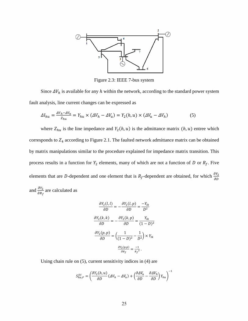
Figure 2.3: IEEE 7-bus system
Since 𝛥𝑉ℎ is available for any ℎ within the network, according to the standard power system
fault analysis, line current changes can be expressed as
𝛥𝐼ℎ𝑢 =𝛥𝑉ℎ−𝛥𝑉𝑢
𝑍ℎ𝑢= 𝑌ℎ𝑢 × (𝛥𝑉ℎ − 𝛥𝑉𝑢) = 𝑌2(ℎ, 𝑢) × (𝛥𝑉𝑢 − 𝛥𝑉ℎ) (5)
where 𝑍ℎ𝑢 is the line impedance and 𝑌2(ℎ, 𝑢) is the admittance matrix (ℎ, 𝑢) entree which
corresponds to 𝑍4 according to Figure 2.1. The faulted network admittance matrix can be obtained
by matrix manipulations similar to the procedure explained for impedance matrix transition. This
process results in a function for 𝑌2 elements, many of which are not a function of 𝐷 or 𝑅𝑓. Five
elements that are 𝐷-dependent and one element that is 𝑅𝑓-dependent are obtained, for which 𝜕𝑌2
𝜕𝐷
and 𝜕𝑌2
𝜕𝑅𝑓 are calculated as
𝜕𝑌2(𝑙, 𝑙)
𝜕𝐷= −
𝜕𝑌2(𝑙, 𝑝)
𝜕𝐷=
−𝑌𝑙𝑘
𝐷2
𝜕𝑌2(𝑘, 𝑘)
𝜕𝐷= −
𝜕𝑌2(𝑘, 𝑝)
𝜕𝐷=
𝑌𝑙𝑘
(1 − 𝐷)2
𝜕𝑌2(𝑝, 𝑝)
𝜕𝐷= (
1
(1 − 𝐷)2−
1
𝐷2) × 𝑌𝑙𝑘
𝜕𝑌2(𝑝,𝑝)
𝜕𝑅𝑓=
−1
𝑅𝑓2 .
Using chain rule on (5), current sensitivity indices in (4) are
𝑆ℎ𝑢,𝐹𝐷𝐼 = (
𝜕𝑌2(ℎ, 𝑢)
𝜕𝐷(𝛥𝑉ℎ − 𝛥𝑉𝑢) + (
𝜕𝛥𝑉𝑢𝜕𝐷
−𝜕𝛥𝑉ℎ
𝜕𝐷)𝑌ℎ𝑢)
−1

26
𝑆ℎ𝑢,𝐹
𝑅𝑓𝐼= (
𝜕𝑌2(ℎ,𝑢)
𝜕𝑅𝑓(𝛥𝑉ℎ − 𝛥𝑉𝑢) + (
𝜕𝛥𝑉𝑢
𝜕𝑅𝑓−
𝜕𝛥𝑉ℎ
𝜕𝑅𝑓) 𝑌ℎ𝑢)
−1
.
It should be mentioned that for cases where fault is on the line whose current is measured,
𝑆ℎ𝑝,𝐹𝐷𝐼 and 𝑆ℎ𝑝,𝐹
𝑅𝑓𝐼 are calculated with 𝑝 = 𝑛 + 1 due to an additional bus at the fault location.
Equations (3) and (4) present observant bus ℎ voltage and current sensitivity indices with
respect to fault location 𝐷 and impedance 𝑅𝑓 for any fault 𝐹 = (𝑙𝑓 , 𝐷, 𝑅𝑓). Let 𝐹(𝑙𝑓) = (𝑙𝑓 , . , . )
represent all faults on system line 𝑙𝑓 with varying 0 ≤ 𝐷 ≤ 1 and 0 ≤ 𝑅𝑓 ≤ 𝑅𝑚𝑎𝑥. Therefore,
𝑆ℎ,𝐹(𝑙𝑓)𝐷𝑉 , 𝑆
ℎ,𝐹(𝑙𝑓)
𝑅𝑓𝑉, 𝑆ℎ𝑢,𝐹(𝑙𝑓)
𝐷𝐼 , and 𝑆ℎ𝑢,𝐹(𝑙𝑓)
𝑅𝑓𝐼are observant bus ℎ sensitivity indices for all possible faults
on line 𝑙𝑓. Hence, all observant bus (ℎ) measurement sensitivities can be evaluated for all possible
faulty lines (𝑙𝑓). Subsequently, any observant bus ℎ measurement can be qualified to detect faults
on a group of system lines, and the final possible PMU set should be optimized in a way to cover
all system lines regarding measurement sensitivity for fault detection. On the other hand, a unique
function mapping between the PMU set’s measurements and system faults is possible as long as
there is no multi-estimation. Multi-estimation is a condition where different faults in the power
system cause similar measured values in a set of observant buses with available precisions.
Exhaustive search is used in this chapter to guarantee that the selected PMU set’s measurements,
that satisfy the sensitivity criteria, have distinguishable values for all possible faults throughout
the power system.
Definition: Consider an observant set 𝐻 ⊆ {1,2, … ,𝑁}. Measurement set 𝑀𝐻𝐹
corresponding to fault 𝐹 is defined as 𝑀𝐻𝐹 = {𝛥𝑉ℎ,𝐹, 𝛥𝐼ℎ𝑢,𝐹|ℎ ∈ 𝐻, 𝑢 ∈ 𝑈ℎ} where 𝑈ℎ is an
adjacent set to observant bus ℎ.
27
1.5. Sensitivity Analysis Criteria for OPP for Fault Location and
Observability
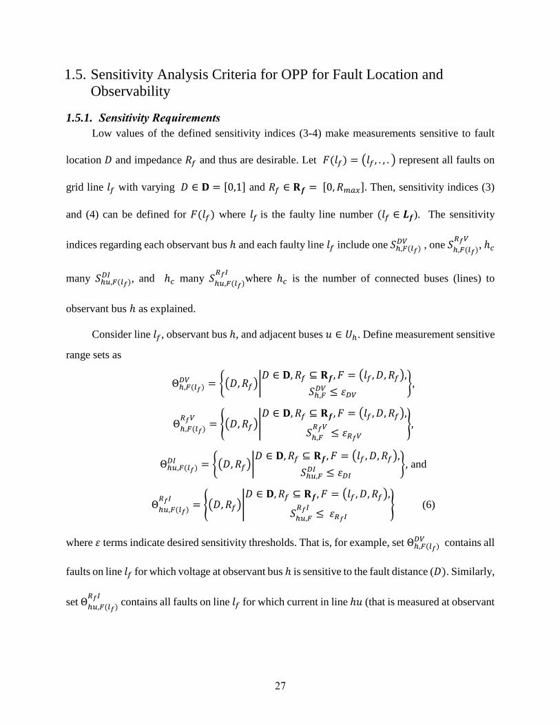
1.5.1. Sensitivity Requirements
Low values of the defined sensitivity indices (3-4) make measurements sensitive to fault
location 𝐷 and impedance 𝑅𝑓 and thus are desirable. Let 𝐹(𝑙𝑓) = (𝑙𝑓 , . , . ) represent all faults on
grid line 𝑙𝑓 with varying 𝐷 ∈ 𝐃 = [0,1] and 𝑅𝑓 ∈ 𝐑𝒇 = [0, 𝑅𝑚𝑎𝑥]. Then, sensitivity indices (3)
and (4) can be defined for 𝐹(𝑙𝑓) where 𝑙𝑓 is the faulty line number (𝑙𝑓 ∈ 𝑳𝒇). The sensitivity
indices regarding each observant bus ℎ and each faulty line 𝑙𝑓 include one 𝑆ℎ,𝐹(𝑙𝑓)𝐷𝑉 , one 𝑆
ℎ,𝐹(𝑙𝑓)
𝑅𝑓𝑉, ℎ𝑐
many 𝑆ℎ𝑢,𝐹(𝑙𝑓)𝐷𝐼 , and ℎ𝑐 many 𝑆
ℎ𝑢,𝐹(𝑙𝑓)
𝑅𝑓𝐼where ℎ𝑐 is the number of connected buses (lines) to
observant bus ℎ as explained.
Consider line 𝑙𝑓, observant bus ℎ, and adjacent buses 𝑢 ∈ 𝑈ℎ. Define measurement sensitive
range sets as
Θℎ,𝐹(𝑙𝑓)𝐷𝑉 = {(𝐷, 𝑅𝑓)|
𝐷 ∈ 𝐃, 𝑅𝑓 ⊆ 𝐑𝒇, 𝐹 = (𝑙𝑓 , 𝐷, 𝑅𝑓),
𝑆ℎ,𝐹𝐷𝑉 ≤ 𝜀𝐷𝑉
},
Θℎ,𝐹(𝑙𝑓)
𝑅𝑓𝑉= {(𝐷, 𝑅𝑓)|
𝐷 ∈ 𝐃, 𝑅𝑓 ⊆ 𝐑𝒇, 𝐹 = (𝑙𝑓 , 𝐷, 𝑅𝑓),
𝑆ℎ,𝐹
𝑅𝑓𝑉≤ 𝜀𝑅𝑓𝑉
},
Θℎ𝑢,𝐹(𝑙𝑓)𝐷𝐼 = {(𝐷, 𝑅𝑓)|
𝐷 ∈ 𝐃, 𝑅𝑓 ⊆ 𝐑𝒇, 𝐹 = (𝑙𝑓 , 𝐷, 𝑅𝑓),
𝑆ℎ𝑢,𝐹𝐷𝐼 ≤ 𝜀𝐷𝐼
}, and
Θℎ𝑢,𝐹(𝑙𝑓)
𝑅𝑓𝐼= {(𝐷, 𝑅𝑓)|
𝐷 ∈ 𝐃, 𝑅𝑓 ⊆ 𝐑𝒇, 𝐹 = (𝑙𝑓 , 𝐷, 𝑅𝑓),
𝑆ℎ𝑢,𝐹
𝑅𝑓𝐼≤ 𝜀𝑅𝑓𝐼
} (6)
where 𝜀 terms indicate desired sensitivity thresholds. That is, for example, set Θℎ,𝐹(𝑙𝑓)𝐷𝑉 contains all
faults on line 𝑙𝑓 for which voltage at observant bus ℎ is sensitive to the fault distance (𝐷). Similarly,
set Θℎ𝑢,𝐹(𝑙𝑓)
𝑅𝑓𝐼 contains all faults on line 𝑙𝑓 for which current in line ℎ𝑢 (that is measured at observant

28
bus ℎ) is sensitive to the fault impedance (𝑅𝑓). Now, define, Θℎ,𝐹(𝑙𝑓)𝐷 = Θℎ,𝐹(𝑙𝑓)
𝐷𝑉 ∪
( ∪𝑢∈𝑈ℎ
Θℎ𝑢,𝐹(𝑙𝑓)𝐷𝐼 ), Θ
ℎ,𝐹(𝑙𝑓)
𝑅𝑓 = Θℎ,𝐹(𝑙𝑓)
𝑅𝑓𝑉∪ ( ∪
𝑢∈𝑈ℎ
Θℎ𝑢,𝐹(𝑙𝑓)
𝑅𝑓𝐼), and Θℎ,𝐹(𝑙𝑓) = Θℎ,𝐹(𝑙𝑓)
𝐷 ∩ Θℎ,𝐹(𝑙𝑓)
𝑅𝑓.
Set Θℎ,𝐹(𝑙𝑓)𝐷 includes all faults on line 𝑙𝑓 with fault distances for which voltage or some current
measurements at observant bus ℎ are sensitive to. Similarly, set Θℎ,𝐹(𝑙𝑓)
𝑅𝑓 includes all faults on line
𝑙𝑓 with fault impedances for which voltage or some current measurements at observant bus ℎ are
sensitive to. Set Θℎ,𝐹(𝑙𝑓) includes all faults on line 𝑙𝑓 with distances and impedances for which
voltage or some current measurements at observant bus ℎ are sensitive to. Set Θℎ,𝐹(𝑙𝑓) may include
all or some faults of interest on line 𝑙𝑓 for ∃𝑙𝑓 ∈ 𝑳𝒇. Thus, in general, additional observant buses
must be used to include all faults of interest on all system lines; i.e., for ∀𝑙𝑓 ∈ 𝑳𝒇.
Fault location (for all faults 𝐹) is possible if an observant set can find all faults in regions 𝐃 × 𝐑𝐟
for all power system lines. That is, for any faulty line 𝑙𝑓 ∈ 𝑳𝒇, there must exist an observant set 𝐻
such that ∪ℎ∈𝐻
Θℎ,𝐹(𝑙𝑓) = 𝐃 × 𝐑𝐟 .
In practice, realization of such condition may be difficult, especially for high values of fault
impedance, and thus, a slightly simpler (and probably more conservative) approach is selected here
to simplify calculations. In this research it is an objective to select observant buses that are able to
locate at least 90% of all possible faults in region 𝐃 × 𝐑𝐟 on each faulty line 𝑙𝑓 ∈ 𝑳𝒇. This criterion
is selected based on experience and to add some flexibility in observant bus selection.
Consequently, due to piecewise continuity of the sets defined above, an observant bus ℎ is chosen
if for ∃𝑙𝑓 ∈ 𝑳𝒇 = {1,2, …𝐿} condition (7-a) or (7-b) is satisfied:
𝑆𝑉𝐼𝐷 = (∬ 𝑑𝐷𝑑𝑅𝑓Θℎ,𝐹(𝑙𝑓)
𝐷𝑉 ≥ 𝑆𝐷𝑅) ∨ ( ∨𝑢∈𝑈ℎ
(∬ 𝑑𝐷𝑑𝑅𝑓Θℎ𝑢,𝐹(𝑙𝑓)
𝐷𝐼 ≥ 𝑆𝐷𝑅)) (7-a)
29
𝑆𝑉𝐼𝑅𝑓 = (∬ 𝑑𝐷𝑑𝑅𝑓Θ
ℎ,𝐹(𝑙𝑓)
𝑅𝑓𝑉 ≥ 𝑆𝐷𝑅) ∨ ( ∨𝑢∈𝑈ℎ
(∬ 𝑑𝐷𝑑𝑅𝑓Θℎ𝑢,𝐹(𝑙𝑓)
𝑅𝑓𝐼 ≥ 𝑆𝐷𝑅)) (7-b)
where 𝑆𝐷𝑅 = 0.9∬ 𝑑𝐷𝑑𝑅𝑓𝐃×𝐑𝐟= 0.9𝑅𝑚𝑎𝑥. Condition SVID implies that observant bus ℎ is
sensitive to the distance of 90% of the faults, indicated by region 𝐃 × 𝐑𝐟, on line 𝑙𝑓. Similarly,
SVIRf implies that observant bus ℎ is sensitive to the impedance of 90% of the faults indicated
by region 𝐃 × 𝐑𝐟 on line 𝑙𝑓. Subsequently,
𝑆𝑉𝐼𝐷𝑅𝑓 = 𝑆𝑉𝐼𝐷 ˄ 𝑆𝑉𝐼𝑅𝑓 (8)
with binary value 𝑆𝑉𝐼𝐷𝑅𝑓, is used to determine if observant bus h is capable of illustrate (using
its measurements) the changes in distance and/or impedance of a vast majority of the faults of
interest that occur on line 𝑙𝑓 with the desired precisions indicated by (6). Condition (8) will be
checked for all the power system lines to find observant bus ℎ’s domain of fault coverage. This
step will reduce the number of required observant buses in obtaining fault observability in the
entire system. In practice, one observant bus may not cover the faults on all the power system lines
and thus other observant buses must be exploited so that faulty lines that are not observed by one
observant bus are observed by others. Thus, the above process is repeated for all the power
system’s buses to lay out an initial mapping between the faults of interest and the power system
buses as observant buses. A group of observant buses; i.e., an observant set, if one exists, that
satisfies condition (8) for all 𝑙𝑓 ∈ 𝑳𝒇 provides a solution to the fault location problem and thus
renders the power system fault observable. This is equivalent to an observant set whose
measurements (measurement set) are sensitive to 90% of distances or impedances of the faults on
all power system lines.
30
1.5.2. Uniqueness and Multi Estimation
After finding sensitive bus locations for measurement allocation, multi estimation is a
necessary criterion to check in order to assure that a measurement set is capable of locating all
possible faults in the power system uniquely. The ability of precisely locating a fault in the system,
depends on distinguishable measurements for any two different faults in the system.
Multi estimation exists if for an observant set 𝐻 ⊆ {1,2, … ,𝑁} and two faults 𝐹1 = (𝑙𝑓1, 𝐷1, 𝑅𝑓1)
and 𝐹2 = (𝑙𝑓2, 𝐷2, 𝑅𝑓2) where 𝐹1 ≠ 𝐹2 all corresponding measurements from the observant set 𝐻
are the same; i.e., 𝑀𝐻𝐹1= 𝑀𝐻𝐹2
(See Section II). Analytically, for any pair of faulty lines 𝑙𝑓1, 𝑙𝑓2 ∈
𝑳𝒇 and observant bus ℎ ∈ 𝐻, this results in the following nonlinear equalities in terms of
𝐷1, 𝑅𝑓1, 𝐷2, and 𝑅𝑓2 for ∀𝑢 ∈ 𝑈ℎ:
{𝛥𝑉ℎ,𝐹1
− 𝛥𝑉ℎ,𝐹2= 0
𝛥𝐼ℎ𝑢,𝐹1− 𝛥𝐼ℎ𝑢,𝐹2
= 0 . (9)
Total number of faulty line pairs (𝑙𝑓1, 𝑙𝑓2 ∈ 𝑳𝒇) is 𝐿(𝐿+1)
2 where 𝐿 is the number of power
lines in the power system. This number includes combinations of any two different lines plus the
number of power system lines (L) in order to account for multi estimations on the individual lines.
Thus, for each observant bus ℎ in set 𝐻, (9) represents 𝐿(𝐿+1)
2(ℎ𝑐 + 1) many equations, where ℎ𝑐
is the number of connected buses (lines) to observant bus ℎ as explained in Section II. For unique
fault location and fault observability, multi estimation must not occur. That is, for 𝑙𝑓1 ≠ 𝑙𝑓2, (9)
must result in no solutions whereas for 𝑙𝑓1 = 𝑙𝑓2, it must yield 𝐷1 = 𝐷2 and 𝑅𝑓1 = 𝑅𝑓2. Equations
(9) can be formed by employing (1) and (5) that lead to nonlinear equations that can be solved
numerically.
This approach in the simplest form can represented as an optimization problem in the form
of min(𝑙𝑓,𝐷,𝑅𝑓)
𝑊𝑇𝑋 under constrains (8) and (9) where 𝑋 is an 𝑁 × 1 vector with its elements (0 or 1)
31
represents selection of an observant bus , and 𝑊 = [𝑤1 , 𝑤2, … , 𝑤𝑁]𝑇 is a weight matrix that
reflects practical or operational priorities in selecting observant buses with 0 ≤ 𝑤𝑖 ≤ 1. The cost
function can be developed further to include other constraints such as contingencies, etc., but is
not the objective of this chapter and not further discussed here and thus an exhaustive search is
used to solve the OPP problem.
1.6. Proposed Algorithm for OPP and Artificial Neural Network Fault
Locator
Previous works consider optimal PMU placement with much emphasis on the PMU cost as
a weight vector in the optimization problem. However, measurement precision and bus suitability
for fault observability are mostly neglected in assigning PMU locations [6]–[16]. PMU fault
location capability is a function of its location in the system. Measurement from a PMU installed
in an improper location may cause significant inaccuracy in fault location. The proposed
formulation and algorithm in this chapter aims to thoroughly consider this. Power system buses
have to be checked and conditions (7) and (9) be evaluated to obtain appropriate observant set 𝐻.
These conditions can be evaluated through solving (7) and (9) for all grid buses so that a set of
appropriate observant buses are selected, and can be translated to sensitivity and uniqueness
conditions required for fault observability and location. Numerical solutions can be sought to
evaluate observant buses which are explained next. Before we proceed, the following discussions
are conducted.
Remark (Measurement Precision): IEEE C57.13 standard for instrumentation transformers
suggests 0.3% error for current and voltage transformer [20]-[21]. Since PMU measurement
precision is usually higher than that of the instrumentation, precisions of 1%, and 0.1% are
considered in this study for both current and voltage measurements total vector error (i.e.,

32
𝑇𝑉𝐸𝑉and 𝑇𝑉𝐸𝐼), where 𝑇𝑉𝐸𝑥 = |𝑋𝑚𝑒𝑎𝑠𝑢𝑟𝑒𝑑−𝑋𝑡ℎ𝑒𝑜𝑟𝑖𝑡𝑖𝑐𝑎𝑙
𝑋𝑡ℎ𝑒𝑜𝑟𝑖𝑡𝑖𝑐𝑎𝑙| × 100% [22]. It is worth mentioning that
accurate phasor estimation can be made during fault transients [22]-[25]. Nevertheless, in this
study fault duration is considered to be 0.1 second, which is 6 cycles at 60 Hz and is equal to the
operating time of the circuit breakers. Since the transients caused by the faults are generally
damped within 2 cycles [26], an installed PMU has enough time to measure the steady-state fault
phasors. In case a severe fault occurs at a PMU location, the amplitude of the measured voltage or
current phasors can be very inaccurate; however, the proposed method exploits multiple
measurements across the grid to assure that enough accurate measurements are taken.
Fault Location Precision: Define 𝑇𝑃𝐷 as “target precision for fault distance 𝐷”. Also, define 𝑇𝑃𝑅𝑓
as “target precision for fault resistance 𝑅𝑓”. Note that fault location range is 0 ≤ 𝐷 ≤ 1 on a power
line and thus for a given 𝑇𝑃𝐷 ≤ 1, fault can be located on one of 1
𝑇𝑃𝐷 + 1 equally-spaced points
on any power line. Also, if fault resistance range of interest is 0 ≤ 𝑅𝑓 ≤ 𝑅𝑚𝑎𝑥, for the given 𝑇𝑃𝑅𝑓
the fault resistance can be any of 𝑅𝑚𝑎𝑥
𝑇𝑃𝑅𝑓
+ 1 equally-spaced resistances between 0 and 𝑅𝑚𝑎𝑥.
From the above discussion, the desired upper limits for sensitivity indices (3) and (4) can be
calculated as
𝑆ℎ,𝐹𝐷𝑉 ≤
𝑇𝑃𝐷
𝑇𝑉𝐸𝑉 = 𝜀𝐷𝑉, 𝑆ℎ,𝐹
𝑅𝑓𝑉≤
𝑇𝑃𝑅𝑓
𝑇𝑉𝐸𝑉 = 𝜀𝑅𝑓𝑉, 𝑆ℎ𝑢,𝐹𝐷𝐼 ≤
𝑇𝑃𝐷
𝑇𝑉𝐸𝐼 = 𝜀𝐷𝐼, and 𝑆ℎ𝑢,𝐹
𝑅𝑓𝐼≤
𝑇𝑃𝑅𝑓
𝑇𝑉𝐸𝐼 = 𝜀𝑅𝑓𝐼
(10)
for all ℎ ∈ {1,2, … ,𝑁} and 𝑢 ∈ 𝑈ℎ. For example, for 𝑇𝑃𝐷 = 0.01, 𝑇𝑃𝑅𝑓 = 0.05, 𝑇𝑉𝐸𝑉 = 0.1%,
and 𝑇𝑉𝐸𝐼 = 0.1% one has 𝜀𝐷𝑉 = 10, 𝜀𝑅𝑓𝑉 = 50, 𝜀𝐷𝐼 = 10, and 𝜀𝑅𝑓𝐼 = 50.
So far, the relationship between sensitivity indices (3) and (4) and the fault location and impedance
accuracy is explained. Thresholds (10) can be utilized to evaluate the quality of observant bus ℎ.
Once the sensitivity measures (3) and (4) are obtained as functions of fault 𝐹 = (𝑙𝑓 , 𝐷, 𝑅𝑓), they
can be compared with thresholds (10) across all variations of faulty line 𝑙𝑓, location 𝐷, and

33
impedance 𝑅𝑓 to determine if observant bus ℎ is a good choice. In addition, conditions to check
the multi estimation are introduced. The algorithm to find optimal PMU sets introduced, which
comes next.
Proposed Algorithm
1) Enter the algorithm inputs: 𝑇𝑃𝐷, 𝑇𝑃𝑅𝑓, 𝑇𝑉𝐸𝑉, 𝑇𝑉𝐸𝐼 and 𝑆𝐷𝑅. Calculate the sensitivity
thresholds 𝜀𝐷𝑉, 𝜀𝑅𝑓𝑉, 𝜀𝐷𝐼 and 𝜀𝑅𝑓𝐼 using (10).
2) Select an observant bus ℎ and a faulty line 𝑙𝑓 ∈ 𝑳𝒇 and obtain the sensitivity indices (3) and
(4) for fault 𝐹 = (𝑙𝑓 , 𝐷, 𝑅𝑓) for all 𝐷 ∈ 𝐃 and 𝑅𝑓 ∈ 𝐑𝒇 with (target precisions) 𝑇𝑃𝐷 and 𝑇𝑃𝑅𝑓
steps, respectively. That is, sensitivity indices are evaluated on all 1
𝑇𝑃𝐷 + 1 equally-spaced
points on line 𝑙𝑓 and all the 𝑅𝑚𝑎𝑥
𝑇𝑃𝑅𝑓
+ 1 equally-spaced resistances between 0 and 𝑅𝑚𝑎𝑥.
3) Obtain sensitivity ranges (6) by comparing the sensitivity indices of Step 2 with thresholds
𝜀𝐷𝑉, 𝜀𝑅𝑓𝑉, 𝜀𝐷𝐼 and 𝜀𝑅𝑓𝐼 of Step 1.
4) Check sensitivity criteria (ability to find the fault distance and impedance with desired
accuracies 𝑇𝑃𝐷 and 𝑇𝑃𝑅𝑓 of Step 1) of observant bus ℎ for fault location on line 𝑙𝑓 through
evaluating (7-a), (7-b), and (8).
5) Repeat Steps 2 to 4 for all lines 𝑙𝑓 ∈ {1,2, … , 𝐿} and store the lines for which fault distance and
impedance can be determined with desired accuracy using observant bus ℎ . This step also
determines how many faulty lines are observable by observant bus ℎ (rank of bus ℎ).
6) Repeat Step 5 for all observant buses ℎ ∈ {1,2, … ,𝑁}.
7) Form all possible observant sets passing sensitivity criteria. An individual observant bus may
not satisfy criteria (8) for all faults of interest in the power system. That is, not all faulty lines
may be observable by an individual observant bus due to missing some fault locations or

34
impedances. However, a set of observant buses (that may not be unique) may be capable of
observing all faulty lines; that is, there may exist an observant set that satisfy criterion (8) for
all grid lines. Such an observant set is capable of finding faulty lines, distances, and impedances
of all faults through various voltage and current measurements. In many power systems a trivial
set of such observant set is the entirety of the power system buses. However, in the majority
of power systems, a smaller number of observant buses forming an observant set can serve and
observe all faulty lines (determining fault locations and impedances). In this step, combinations
of observant buses forming such observant sets, with minimum number of observant buses
obtained and saved. This starts by examining one-observant-bus sets, two-observant-bus sets,
three-observant-bus sets, etc. As soon as an observant set that satisfies (8) is found, one optimal
observant set is obtained to be checked against multi estimation.
8) Check for multi estimation. Each observant set obtained in Step 7 must be checked against
multi estimation. Select an observant set (obtained in Step 7). Select a pair of faulty lines
𝑙𝑓1, 𝑙𝑓2 ∈ 𝑳𝒇. Equations (9) must yield no solutions but the trivial solution𝐹1 = 𝐹2, for selected
lines 𝑙𝑓1, 𝑙𝑓2 for the measurement set of the selected observant set. Discard the measurement
set if equations (9) yield non-trivial solutions; i.e., two faults yield similar measurement sets
in the selected observant set.
9) Repeat Step 8 for all 𝐿(𝐿+1)
2 power line pairs for each set.
10) Collect all the observant sets that pass Step 9. The observant sets with minimum number of
observant buses are chosen as the optimal measurement set(s). This in turn determines the
optimal PMU locations. Among the optimal sets the set with the maximum number of
measurements outperforms and is chosen.
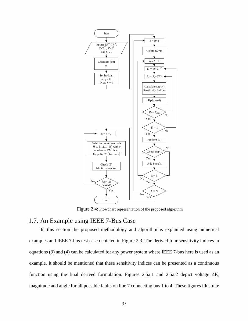
A flowchart of the proposed algorithm is depicted in Figure 2.4 to clarify these steps.
35
Start
Inputs: TPD, TP
Rf,
TVEV , TVE
I
and SDR .
Set Initials.
h, lf = 0,
D, Rf, x = 0
Calculate (3)-(4)
Sensitivity Indices
Update (6)
Perform (7)
Rf = Rmax
h = h+1
lf = lf +1
D = D+TPD
Rf = Rf+TPRf
D = 1
lf = L
h = N
Yes
Yes
Yes
No
No
No
No
x = x +1
Check (9)
Multi Estimation
Any set
passed?
End.
Yes
No
Calculate (10)
εs
Check (8)=1
Yes
Create Ωh=Ø
Add lf to Ωh
No
Yes
Select all observant sets
𝐻 ⊆ {1,2, … , 𝑁} with x
number of PMUs s.t.
𝛺ℎℎ∈𝐻 = {1,2, … , 𝐿}
Figure 2.4: Flowchart representation of the proposed algorithm
1.7. An Example using IEEE 7-Bus Case
In this section the proposed methodology and algorithm is explained using numerical
examples and IEEE 7-bus test case depicted in Figure 2.3. The derived four sensitivity indices in
equations (3) and (4) can be calculated for any power system where IEEE 7-bus here is used as an
example. It should be mentioned that these sensitivity indices can be presented as a continuous
function using the final derived formulation. Figures 2.5a.1 and 2.5a.2 depict voltage 𝛥𝑉4
magnitude and angle for all possible faults on line 7 connecting bus 1 to 4. These figures illustrate
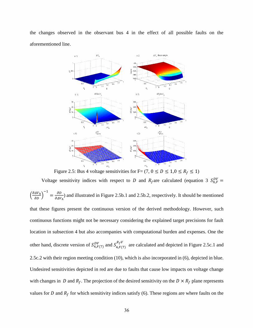
36
the changes observed in the observant bus 4 in the effect of all possible faults on the
aforementioned line.
Figure 2.5: Bus 4 voltage sensitivities for F= (7, 0 ≤ 𝐷 ≤ 1,0 ≤ 𝑅𝑓 ≤ 1)
Voltage sensitivity indices with respect to 𝐷 and 𝑅𝑓are calculated (equation 3 𝑆ℎ,𝐹𝐷𝑉 =
(𝜕𝛥𝑉ℎ
𝜕𝐷)−1
=𝜕𝐷
𝜕𝛥𝑉ℎ) and illustrated in Figure 2.5b.1 and 2.5b.2, respectively. It should be mentioned
that these figures present the continuous version of the derived methodology. However, such
continuous functions might not be necessary considering the explained target precisions for fault
location in subsection 4 but also accompanies with computational burden and expenses. One the
other hand, discrete version of 𝑆4,𝐹(7)𝐷𝑉 and 𝑆
4,𝐹(7)
𝑅𝑓𝑉 are calculated and depicted in Figure 2.5c.1 and
2.5c.2 with their region meeting condition (10), which is also incorporated in (6), depicted in blue.
Undesired sensitivities depicted in red are due to faults that cause low impacts on voltage change
with changes in 𝐷 and 𝑅𝑓. The projection of the desired sensitivity on the 𝐷 × 𝑅𝑓 plane represents
values for 𝐷 and 𝑅𝑓 for which sensitivity indices satisfy (6). These regions are where faults on the
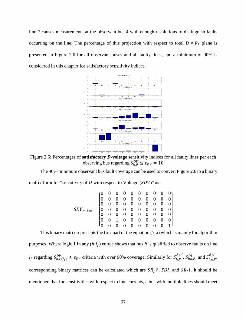
37
line 7 causes measurements at the observant bus 4 with enough resolutions to distinguish faults
occurring on the line. The percentage of this projection with respect to total 𝐷 × 𝑅𝑓 plane is
presented in Figure 2.6 for all observant buses and all faulty lines, and a minimum of 90% is
considered in this chapter for satisfactory sensitivity indices.
Figure 2.6: Percentages of satisfactory 𝑫-voltage sensitivity indices for all faulty lines per each
observing bus regarding 𝑆ℎ,𝐹𝐷𝑉 ≤ 𝜀𝐷𝑉 = 10
The 90% minimum observant bus fault coverage can be used to convert Figure 2.6 to a binary
matrix form for “sensitivity of 𝐷 with respect to Voltage (𝑆𝐷𝑉)” as:
𝑆𝐷𝑉7−𝑏𝑢𝑠 =
[ 0000000
0000000
0000010
0000000
0000000
0000000
0000000
0000000
0000000
0000001]
This binary matrix represents the first part of the equation (7-a) which is mainly for algorithm
purposes. Where logic 1 in any (ℎ,𝑙𝑓) entree shows that bus ℎ is qualified to observe faults on line
𝑙𝑓 regarding 𝑆ℎ,𝐹(𝑙𝑓)𝐷𝑉 ≤ 𝜀𝐷𝑉 criteria with over 90% coverage. Similarly for 𝑆ℎ,𝐹
𝑅𝑓𝑉, 𝑆ℎ𝑢,𝐹
𝐷𝐼 , and 𝑆ℎ𝑢,𝐹
𝑅𝑓𝐼,
corresponding binary matrices can be calculated which are 𝑆𝑅𝑓𝑉, 𝑆𝐷𝐼, and 𝑆𝑅𝑓𝐼. It should be
mentioned that for sensitivities with respect to line currents, a bus with multiple lines should meet
38
the condition mentioned in (6) for at least one of its connected lines measurements. In a similar
way, the binary matrix for qualified observant buses to detect faults on all system lines (first part
of the equation (7-b)) can be calculated as:
𝑆𝑅𝑓𝑉7−𝑏𝑢𝑠 =
[ 0010001
1010001
1000000
0110011
1100000
1100000
0110011
0010001
0100000
1100000]
.
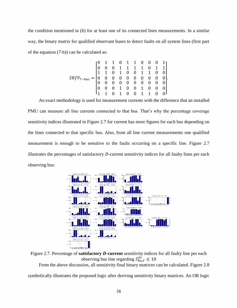
An exact methodology is used for measurement currents with the difference that an installed
PMU can measure all line currents connected to that bus. That’s why the percentage coverage
sensitivity indices illustrated in Figure 2.7 for current has more figures for each bus depending on
the lines connected to that specific bus. Also, from all line current measurements one qualified
measurement is enough to be sensitive to the faults occurring on a specific line. Figure 2.7
illustrates the percentages of satisfactory 𝐷-current sensitivity indices for all faulty lines per each
observing bus:
Figure 2.7. Percentage of satisfactory 𝑫-current sensitivity indices for all faulty line per each
observing bus line regarding 𝑆ℎ𝑢,𝐹𝐷𝐼 ≤ 10
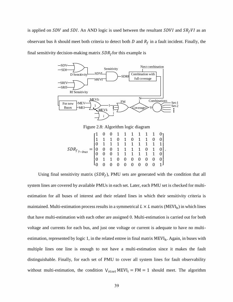
From the above discussion, all sensitivity final binary matrices can be calculated. Figure 2.8
symbolically illustrates the proposed logic after deriving sensitivity binary matrices. An OR logic
39
is applied on 𝑆𝐷𝑉 and 𝑆𝐷𝐼. An AND logic is used between the resultant 𝑆𝐷𝑉𝐼 and 𝑆𝑅𝑓𝑉𝐼 as an
observant bus ℎ should meet both criteria to detect both 𝐷 and 𝑅𝑓 in a fault incident. Finally, the
final sensitivity decision-making matrix 𝑆𝐷𝑅𝑓for this example is
D Sensitivity
Rf Sensitivity
Sensitivity
SDVI
SRfVI
SDV
SDI
SRfV
SRfI
MEV
MEI
SDRf
For new
Buses
MEVI1
1
MEVIi
i
1
i
... Coverage?
Combination with
full coverage
FM
... Y
Set-1Combinations
Set-2
N
Next combination
Figure 2.8: Algorithm logic diagram
𝑆𝐷𝑅𝑓7−𝑏𝑢𝑠=
[ 1100000
0110010
0110010
1011100
1111100
1011100
1111100
1110100
1011100
0010001]
.
Using final sensitivity matrix (𝑆𝐷𝑅𝑓), PMU sets are generated with the condition that all
system lines are covered by available PMUs in each set. Later, each PMU set is checked for multi-
estimation for all buses of interest and their related lines in which their sensitivity criteria is
maintained. Multi-estimation process results in a symmetrical 𝐿 × 𝐿 matrix (MEVIh) in which lines
that have multi-estimation with each other are assigned 0. Multi-estimation is carried out for both
voltage and currents for each bus, and just one voltage or current is adequate to have no multi-
estimation, represented by logic 1, in the related entree in final matrix MEVIh. Again, in buses with
multiple lines one line is enough to not have a multi-estimation since it makes the fault
distinguishable. Finally, for each set of PMU to cover all system lines for fault observability
without multi-estimation, the condition ⋁ MEVIi𝑖∈𝑠𝑒𝑡 = FM = 1 should meet. The algorithm

40
presented in Figure 2.8 halts once first set of PMUs causing full coverage without multi-estimation
is found and provides all possible combinations for this set of PMUs passing the criteria. In the
results provided in the next sections, this is modified to find all possible combination with the
minimum number of PMUs in the sets.
1.8. Artificial Neural Network (ANN) Fault Locator
Once the optimal observant set is obtained, it is assured that the set can locate all faults of
interest uniquely without multi estimation. Thus, a one-to-one map exists between the
corresponding measurement set and the faults of interest (that includes the faulty line, the fault
distance, and impedance). Consequently, artificial neural networks (ANNs) are capable of and
used to map the measurement set (from the optimal observant set) to their related faults comprising
faulty line 𝑙𝑓, distance 𝐷, and resistance 𝑅𝑓. As an example, here we assume that H = {2,3} is an
OPP solution for the IEEE 7-bus example case in previous section. Therefore, resulting
measurements in such set will be 𝑀𝐻𝐹 = {𝛥𝑉ℎ,𝐹, 𝛥𝐼ℎ𝑢,𝐹|ℎ ∈ 𝐻, 𝑢 ∈ 𝑈ℎ} =
{𝑉2, 𝐼2𝑔, 𝐼21, 𝐼26, 𝐼25, 𝑉3, 𝐼3𝑔, 𝐼34, 𝐼35, 𝐼36, 𝐼37}. Therefore, the explained one-to-one function
mapping between all system faults and OPP set measurements can be illustrated using these two
equation which are also visually depicted in Figure 2.9.
𝑓(𝑙𝑓,𝐷, 𝑅𝑓) = 𝑀𝐻𝐹 = (𝑉2, 𝐼2𝑔, 𝐼21, 𝐼26, 𝐼25, 𝑉3, 𝐼3𝑔, 𝐼34, 𝐼35, 𝐼36, 𝐼37)
𝑓(𝑉2, 𝐼2𝑔,𝐼21,𝐼26,𝐼25,𝑉3,𝐼3𝑔,𝐼34,𝐼35,𝐼36,𝐼37)−1 = 𝐹 = (𝑙𝑓 , 𝐷, 𝑅𝑓)
Figure 2.9: IEEE 7-bus test system fault observability using OPP

41
Artificial neural networks are intelligent mechanisms that can approximate complex
nonlinear functions through employing a set of input and output data [27]. The function
approximation property of the ANNs is used here to estimate the function that maps the
measurement set as input and related fault as output. Offline training is used and corresponding
weights and bias values of the ANN are obtained using MATLAB via the Levenberg-Marquardt
optimization method [29] which is an efficient method in training feedforward ANNs. The
artificial neural networks here have one hidden layer and one output layer with sigmoid and linear
activation functions, respectively.
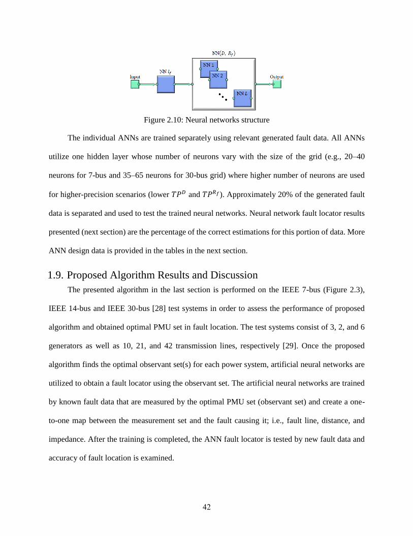
In this study, instead of using one large neural network, a structure of networks is employed
in order to have a more precise fault locator. That is, faulty line 𝑙𝑓 is found in the first neural
network using input data from the measurement set. Then, based on the detected faulty line, a
pertinent neural network is activated to determine fault distance 𝐷, and resistance 𝑅𝑓, as shown in
Figure 2.10. Input vector 𝑋 of the first ANN is the measurement set’s (corresponding to the
obtained OPP) voltage and current magnitudes and angles. Output vector 𝑌1 is the faulty line 𝑙𝑓.
That is, 𝑌1 = 𝑊𝑇 Φ(𝑉𝑇 𝑋) where 𝑊1 is the output layer weight matrix, Phi is the Sigmoid
activation function, and 𝑉1 is the hidden layer weight matrix. Next, a second ANN is selected
corresponding to the resultant faulty line from the first ANN. In the second ANN, the input vector
is 𝑋 as explained and output vector 𝑌2 = [𝐷 𝑅𝑓]𝑇is the location and resistance of the fault located
on faulty line 𝑙𝑓. That is, 𝑌2 = 𝑊𝑙𝑓𝑇 Φ(𝑉𝑙𝑓
𝑇 𝑋) where 𝑊𝑙𝑓 is the output layer weight matrix, Phi is
the Sigmoid activation function, and 𝑉𝑙𝑓 is the hidden layer weight matrix corresponding to faulty
line 𝑙𝑓.
42
Figure 2.10: Neural networks structure
The individual ANNs are trained separately using relevant generated fault data. All ANNs
utilize one hidden layer whose number of neurons vary with the size of the grid (e.g., 20–40
neurons for 7-bus and 35–65 neurons for 30-bus grid) where higher number of neurons are used
for higher-precision scenarios (lower 𝑇𝑃𝐷 and 𝑇𝑃𝑅𝑓). Approximately 20% of the generated fault
data is separated and used to test the trained neural networks. Neural network fault locator results
presented (next section) are the percentage of the correct estimations for this portion of data. More
ANN design data is provided in the tables in the next section.
1.9. Proposed Algorithm Results and Discussion
The presented algorithm in the last section is performed on the IEEE 7-bus (Figure 2.3),
IEEE 14-bus and IEEE 30-bus [28] test systems in order to assess the performance of proposed
algorithm and obtained optimal PMU set in fault location. The test systems consist of 3, 2, and 6
generators as well as 10, 21, and 42 transmission lines, respectively [29]. Once the proposed
algorithm finds the optimal observant set(s) for each power system, artificial neural networks are
utilized to obtain a fault locator using the observant set. The artificial neural networks are trained
by known fault data that are measured by the optimal PMU set (observant set) and create a one-
to-one map between the measurement set and the fault causing it; i.e., fault line, distance, and
impedance. After the training is completed, the ANN fault locator is tested by new fault data and
accuracy of fault location is examined.

43
Fault impedance is considered to be purely resistive in this study [16]. The maximum fault
resistance of the interest is considered to be 𝑅𝑚𝑎𝑥 = 17.4 for all test cases, i.e., 0.1 p.u in 132 kV
base voltage. By increasing the required maximum fault resistance of interest to be detected by an
observant set the number of PMUs in the found set may increase since the set performance is
demanded to cover higher resistance faults. Various voltage and current measurement precisions
are used to solve the OPP problem in order to include various PT and CT precisions.
Table 2.1 presents OPP results for the IEEE 7-bus system. Two cases are performed in the
simulation: with target precisions of 1% for fault distance 𝐷 and resistance 𝑅𝑓, and with target
precisions of 5% for 𝐷 and 𝑅𝑓. These precisions are the desired fault location accuracies here and
thus they are used in generating faults that are used in training and testing the ANN fault locator.
Table 2.1: IEEE 7-bus OPP and ANN results for various target precisions and different
measurements accuracies
IEEE 7-bus OPP (𝑹𝒇max 0.1 pu) ANN
𝑇𝑉𝐸𝑉 𝑇𝑉𝐸𝐼 #
PMUs
Optimal observant sets
(PMU locations)
Percentage estimation accuracy
𝑙𝑓 D
(ave)
(min)
Rf (ave)
(min)
𝑻𝑷𝑫 = 𝟎. 𝟎𝟏, 𝑻𝑷𝑹𝒇 = 𝟎. 𝟎𝟏, Total generated faults: 11000
10-2 10-2 2 (1,2)-(2,3) 99.6 99.9
99.1
99.9
99.5
10-3 10-2 2 (1,2)-(2,3) 99.8 100 100
100 100
10-3 10-3 1 (1)-(2)-(3)-(5) 99.9 100
100
100
100
𝑻𝑷𝑫 = 𝟎. 𝟎𝟓, 𝑻𝑷𝑹𝒇 = 𝟎. 𝟎𝟓, Total generated faults: 600
10-2 10-2 1 (3)-(5) 99.1 99.1 91.6
100 100
10-3 10-2 1 (3)-(5) 99.1 99.1
91.6
100
100
10-3 10-3 1 (1)-(2)-(3)-(4)-(5)-(6) 100 99.1 91.6
100 100
The first two columns of Table 2.1 show voltage and current measurement precisions. These
precisions are used in solving the OPP in the proposed algorithm where sensitivity indices are
utilized. Columns 3 and 4 represent the minimum number of required PMUs and the optimal
observant set(s) that the proposed algorithm suggests. The artificial neural network fault locator is

44
trained by employing the optimal observant set shown in bold. For the case with 1% target
precisions for 𝐷 and 𝑅𝑓, 11,000 fault scenarios are generated throughout the system and used for
ANN training and 2,200 fault data are used for test and validation. Similarly, for the case with 5%
target precision for 𝐷 and 𝑅𝑓, 600 fault scenarios are used for training and 120 fault scenarios are
used for validation. The remaining columns show the accuracy of fault location using the trained
ANN fault locator. The fault locator has dedicated artificial neural networks for each line in its
second stage and after the faulty line is found as shown in Fig. 5. The top and bottom percentage
values in the last two columns show the average and minimum estimation accuracies, respectively,
across all network lines. One can observe that by using current and voltage precision of 10-2 (1%)
only two optimal observant sets with 2 PMUs in each set are found by the proposed algorithm.
The minimum number of PMUs and the optimal observant sets remain the same by increasing only
the voltage precision to 10-3. However, when increasing the current measurement precision to 10-
3 (0.1%) only one PMU is enough for the system to be fault observable. On the other hand, by
reducing the preferred precision for the fault location (the target precision of 5%), only one PMU
is capable of observing all system faults.
Tables 2.2 and 2.3 present the results of the proposed OPP and ANN locators for IEEE 14-
bus and 30-bus systems. The bus numbers given in [28] are adopted here for the power systems. It
is observed that higher current measurement precision is more effective than that of voltage in
reducing the number of required PMUs as shown in the tables. Overall, these results show the
impact of measurement precision on OPP solutions which is detailed for the first time here. In
addition, provided results illustrate a significant improvement over the conventional one-bus-
spaced method where approximately 50% of buses are required for the system fault observability
[7], [15]. For example the number of suggested PMUs for one-bus-spaced method is 17 [15] for

45
the IEEE 30-bus system as opposed to 13 PMUs obtained here using 10-2 measurement precision.
Moreover, [15] proposes 14 PMUs for the IEEE 30-bus system when considering 6 zero-injection
buses (that reduce grid size) and [7] proposes 8 PMUs using 15 additional flow measurements.
By contrast, the proposed algorithm suggests 13 PMUs using 10-2 measurement precision and 2
PMUs using 10-3 measurement precision with the desired fault location accuracy of 1% for both
fault distance and impedance. Table 2.4 summarizes the results of references [7] and [15] that
employ Integer Linear Programming (ILP) in the context of one-bus-spaced strategy for full
system fault observability. Note that the measurement precision is not considered and elaborated
in these works whereas the precision plays an important role in the number of required
measurement units. That is, higher fault location and/or impedance precision need larger numbers
of employed PMUs.
Table 2.2: IEEE 14-bus OPP and ANN results for various target precisions and different
measurements accuracies
IEEE 14-bus OPP (𝑹𝒇max 0.1 pu) ANN
𝑇𝑉𝐸𝑉 𝑇𝑉𝐸𝐼 #
PMUs Optimal observant sets
(PMU locations)
Percentage
estimation accuracy
𝑙𝑓 D
(ave)
(min)
Rf (ave)
(min)
𝑻𝑷𝑫 = 𝟎. 𝟎𝟏, 𝑻𝑷𝑹𝒇 = 𝟎. 𝟎𝟏, Total generated faults: 22000
10-2 10-2 7
(2,5,7,9,12,13,14)- (2,5,8,9,12,13,14)-
(2,6,7,9,12,13,14)-
(2,6,8,9,12,13,14)- (2,7,9,11,12,13,14)-
(2,8,9,11,12,13,14)
99.6 99.9
96.1
100
100
10-3 10-2 3 (2,6,9)-(2,9,12)-
(2,9,13) 99.5
99.9
99.1
99.9
99.1
10-3 10-3 1 5 98.2 99.9
99.5
100
100
𝑻𝑷𝑫 = 𝟎. 𝟎𝟓, 𝑻𝑷𝑹𝒇 = 𝟎. 𝟎𝟓, Total generated faults: 1200
10-2 10-2 2 (2,6)-(2,12)-(2,13)
(5,6)-(5,12)-(5,13) 96.7
100
100
100
100
10-3 10-2 2
(1,6)-(2,6)-(2,10)-
(2,11)-(2,12)-(2,13)-
(2,14)-(5,6)-(5,10)- (5,11)-(5,12)-(5,13)-
(5,14)
96.3 100
100
100
100
10-3 10-3 1 1-2-3-4-5 97.1 100
100
100
100
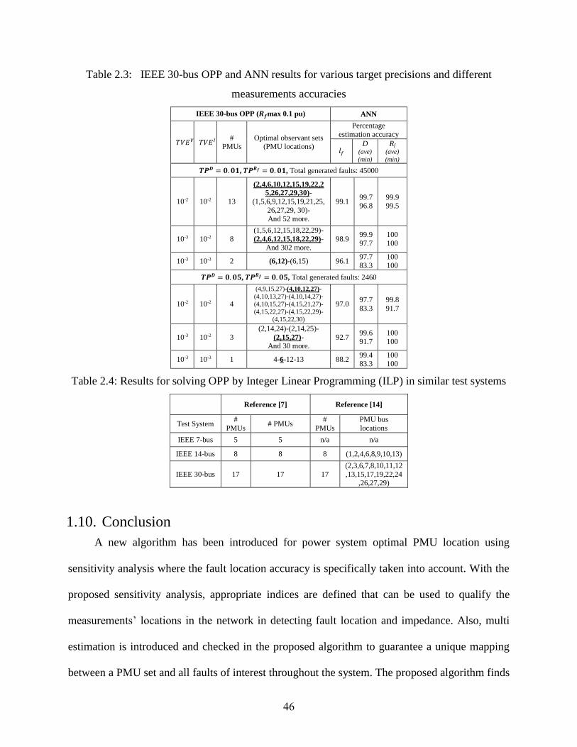
46
Table 2.3: IEEE 30-bus OPP and ANN results for various target precisions and different
measurements accuracies
IEEE 30-bus OPP (𝑹𝒇max 0.1 pu) ANN
𝑇𝑉𝐸𝑉 𝑇𝑉𝐸𝐼 #
PMUs Optimal observant sets
(PMU locations)
Percentage
estimation accuracy
𝑙𝑓 D
(ave)
(min)
Rf (ave)
(min)
𝑻𝑷𝑫 = 𝟎. 𝟎𝟏, 𝑻𝑷𝑹𝒇 = 𝟎. 𝟎𝟏, Total generated faults: 45000
10-2 10-2 13
(2,4,6,10,12,15,19,22,2
5,26,27,29,30)-
(1,5,6,9,12,15,19,21,25,
26,27,29, 30)- And 52 more.
99.1 99.7 96.8
99.9 99.5
10-3 10-2 8
(1,5,6,12,15,18,22,29)-
(2,4,6,12,15,18,22,29)- And 302 more.
98.9 99.9
97.7
100
100
10-3 10-3 2 (6,12)-(6,15) 96.1 97.7
83.3
100
100
𝑻𝑷𝑫 = 𝟎. 𝟎𝟓, 𝑻𝑷𝑹𝒇 = 𝟎. 𝟎𝟓, Total generated faults: 2460
10-2 10-2 4
(4,9,15,27)-(4,10,12,27)- (4,10,13,27)-(4,10,14,27)-
(4,10,15,27)-(4,15,21,27)-
(4,15,22,27)-(4,15,22,29)-
(4,15,22,30)
97.0 97.7
83.3
99.8
91.7
10-3 10-2 3
(2,14,24)-(2,14,25)-
(2,15,27)- And 30 more.
92.7 99.6
91.7
100
100
10-3 10-3 1 4-6-12-13 88.2 99.4
83.3
100
100
Table 2.4: Results for solving OPP by Integer Linear Programming (ILP) in similar test systems
Reference [7] Reference [14]
Test System #
PMUs # PMUs
#
PMUs
PMU bus
locations
IEEE 7-bus 5 5 n/a n/a
IEEE 14-bus 8 8 8 (1,2,4,6,8,9,10,13)
IEEE 30-bus 17 17 17
(2,3,6,7,8,10,11,12
,13,15,17,19,22,24,26,27,29)
1.10. Conclusion
A new algorithm has been introduced for power system optimal PMU location using
sensitivity analysis where the fault location accuracy is specifically taken into account. With the
proposed sensitivity analysis, appropriate indices are defined that can be used to qualify the
measurements’ locations in the network in detecting fault location and impedance. Also, multi
estimation is introduced and checked in the proposed algorithm to guarantee a unique mapping
between a PMU set and all faults of interest throughout the system. The proposed algorithm finds
47
the minimum number of PMUs required for system fault observability. By using the obtained
optimal PMU sets, an artificial neural network fault locator is generated using artificial neural
networks that map between the measurements of the optimal measurement set and the system
faults.
1.11. References
[1] Phadke, A.G., "Synchronized phasor measurements in power systems," Comp. App. in
Pow., IEEE , vol.6, no.2, pp.10-15, 1993.
[2] Baldwin, T.L.; Mili, L.; Boisen, M.B., Jr.; Adapa, R., "Power system observability with
minimal phasor measurement placement," Power Systems, IEEE Transactions on ,
vol.8, no.2, pp.707-715, May 1993.
[3] Bei Xu; Abur, A., "Observability analysis and measurement placement for systems
with PMUs," Power Systems Conference and Exposition, 2004. IEEE PES , vol., no.,
pp.943-946 vol.2, 10-13 Oct. 2004.
[4] Novosel, D.; Madani, V.; Bhargava, B.; Khoi Vu; Cole, J., "Dawn of the grid
synchronization," Power and Energy Magazine, IEEE , vol.6, no.1, pp.49-60, January-
February 2008.
[5] Albuquerque, R.J.; Paucar, V.L., "Evaluation of the PMUs Measurement Channels
Availability for Observability Analysis," Power Systems, IEEE Transactions on ,
vol.28, no.3, pp.2536-2544, 2013.
[6] Quanyuan Jiang; Xingpeng Li; Bo Wang; Haijiao Wang, "PMU-Based Fault Location
Using Voltage Measurements in Large Transmission Networks," Power Delivery,
IEEE Transactions on , vol.27, no.3, pp.1644-1652, July 2012.
[7] Kavasseri, R.; Srinivasan, S.K., "Joint placement of phasor and conventional power
flow measurements for fault observability of power systems," Generation,
Transmission & Distribution, IET , vol.5, no.10, pp.1019-1024, October 2011.
[8] Aminifar, F.; Khodaei, A.; Fotuhi-Firuzabad, M.; Shahidehpour, M., "Contingency-
Constrained PMU Placement in Power Networks," Power Systems, IEEE Transactions
on , vol.25, no.1, pp.516-523, Feb. 2010.
[9] Bei Gou; Kavasseri, R. G., "Unified PMU Placement for Observability and Bad Data
Detection in State Estimation," Power Systems, IEEE Transactions on , vol.29, no.6,
pp.2573-2580, Nov. 2014.
[10] N. C. Koutsoukis, N. M. Manousakis, P. S. Georgilakis and G. N. Korres,
"Numerical observability method for optimal phasor measurement units placement
using recursive Tabu search method," in IET Generation, Transmission & Distribution,
vol. 7, no. 4, pp. 347-356, April 2013.
48
[11] Bei Gou, "Generalized Integer Linear Programming Formulation for Optimal PMU
Placement," Power Systems, IEEE Transactions on , vol.23, no.3, pp.1099-1104, Aug.
2008.
[12] Chakrabarti, S.; Kyriakides, E., "Optimal Placement of Phasor Measurement Units
for Power System Observability," Power Systems, IEEE Transactions on , vol.23, no.3,
pp.1433-1440, Aug. 2008.
[13] Manousakis, N.M.; Korres, G.N.; Georgilakis, P.S., "Taxonomy of PMU
Placement Methodologies," Power Systems, IEEE Transactions on , vol.27, no.2,
pp.1070-1077, May 2012.
[14] Geramian, S.S.; Abyane, H.A.; Mazlumi, K., "Determination of optimal PMU
placement for fault location using genetic algorithm," Harmonics and Quality of
Power, 2008. ICHQP 2008. 13th International Conference on , vol., no., pp.1-5, Sept.
28 2008-Oct. 1 2008.
[15] Pokharel, S.P.; Brahma, S., "Optimal PMU placement for fault location in a power
system," North American Power Symposium (NAPS), 2009 , vol., no., pp.1-5, 4-6 Oct.
2009.
[16] Kai-Ping Lien; Chih-Wen Liu; Chi-Shan Yu; Joe-Air Jiang, "Transmission network
fault location observability with minimal PMU placement," Power Delivery, IEEE
Transactions on , vol.21, no.3, pp.1128-1136, July 2006.
[17] M. Korkali and A. Abur, "Optimal Deployment of Wide-Area Synchronized
Measurements for Fault-Location Observability," in IEEE Transactions on Power
Systems, vol. 28, no. 1, pp. 482-489, Feb. 2013.
[18] M. Korkalı and A. Abur, "Robust Fault Location Using Least-Absolute-Value
Estimator," in IEEE Transactions on Power Systems, vol. 28, no. 4, pp. 4384-4392,
Nov. 2013.
[19] J. J. Grainger, W. D. Stevenson, Power System Analysis, New York: McGraw-Hill,
Inc., International Editions 1994, pp. 283-467.
[20] IEEE Standard Requirements for Instrument Transformers," IEEE Std C57.13-
2008 (Revision of IEEE Std C57.13-1993) , vol., no., pp.c1,82, July 2008.
[21] “Instrument Transformer Technical Information and Application Guide”, ABB
brochure, Doc No. 1VAP420003-TG, Jan. 2005. [Online]. Available:
http://www.abb.com/abblibrary/downloadcenter/?View=Result.
[22] Mai, R.K.; He, Z.Y.; Ling Fu; Kirby, B.; Zhiq Qian Bo, "A Dynamic
Synchrophasor Estimation Algorithm for Online Application," Power Delivery, IEEE
Transactions on , vol.25, no.2, pp.570-578, April 2010.
[23] Rabe, S.; Komarnicki, P.; Styczynski, Z.A.; Gurbiel, M.; Blumschein, J.; Kereit,
M.; Voropai, N., "Automated test procedures for accuracy verification of Phasor
Measurement Units," Power and Energy Society General Meeting, 2012 IEEE , vol.,
no., pp.1-6, 22-26 July 2012.
[24] Rao, J.G.; Pradhan, A.K., "Accurate Phasor Estimation During Power Swing,"
in Power Delivery, IEEE Transactions on , vol.PP, no.99, pp.1-1.

49
[25] Barchi, G.; Macii, D.; Petri, D., "Synchrophasor Estimators Accuracy: A
Comparative Analysis," Inst.and Meas., IEEE Trans. on , vol.62, no.5, pp.963-973,
May 2013.
[26] Watson, N.; Arrillaga, J.; “Power Systems Electromagnetic Transient Simulation”,
IET Power and Energy Series 39.
[27] Salim, R.H.; de Oliveira, K.; Filomena, A.D.; Resener, M.; Bretas, A.S., "Hybrid
Fault Diagnosis Scheme Implementation for Power Distribution Systems Automation,"
in Power Delivery, IEEE Transactions on , vol.23, no.4, pp.1846-1856, Oct. 2008.
[28] Nazaripouya, H.; Mehraeen, S., "Optimal PMU placement for fault observability
in distributed power system by using simultaneous voltage and current
measurements," Power and Energy Society General Meeting (PES), 2013 IEEE , vol.,
no., pp.1-6, 21-25 July 2013.
[29] R. Christie Power System Test Archive,, 1999. [online] Available: http://www.ee.washington.edu/research/pstca.
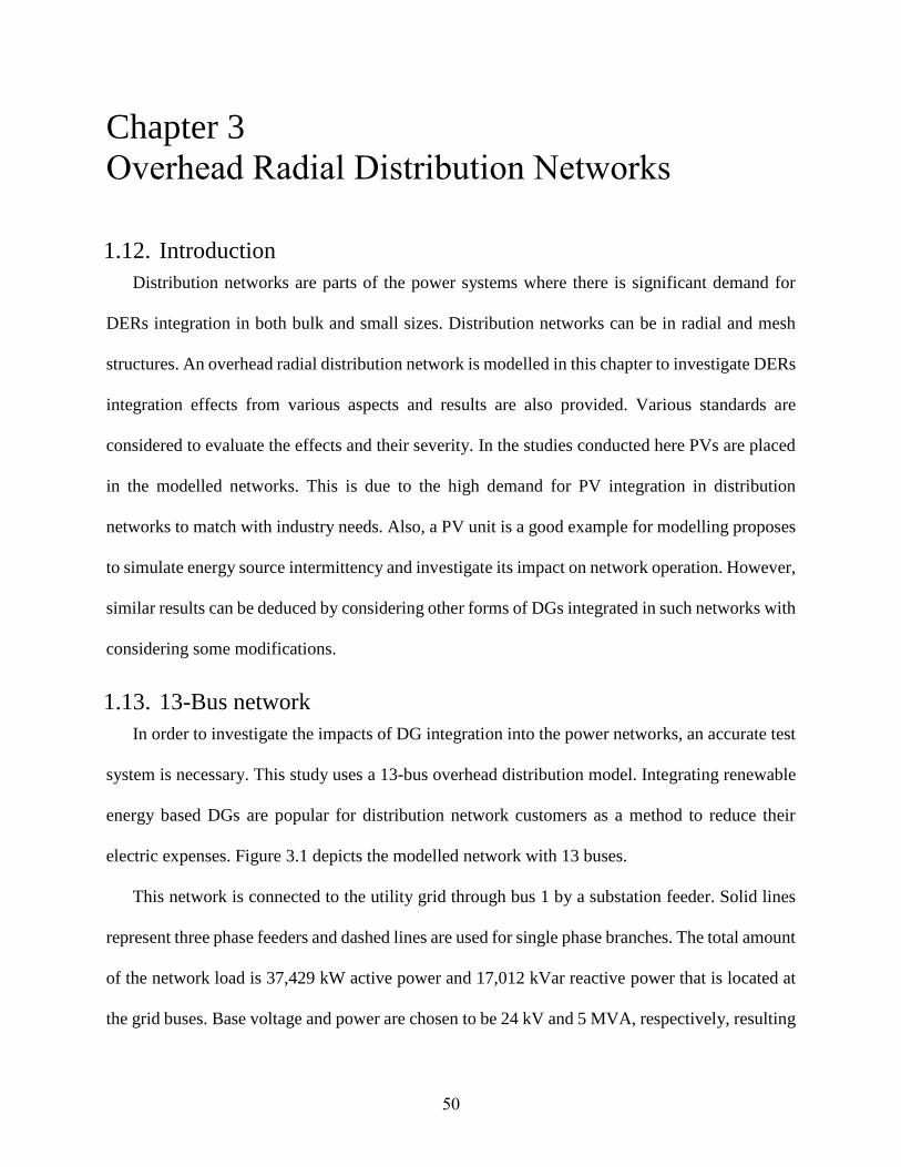
50
Chapter 3
Overhead Radial Distribution Networks
1.12. Introduction
Distribution networks are parts of the power systems where there is significant demand for
DERs integration in both bulk and small sizes. Distribution networks can be in radial and mesh
structures. An overhead radial distribution network is modelled in this chapter to investigate DERs
integration effects from various aspects and results are also provided. Various standards are
considered to evaluate the effects and their severity. In the studies conducted here PVs are placed
in the modelled networks. This is due to the high demand for PV integration in distribution
networks to match with industry needs. Also, a PV unit is a good example for modelling proposes
to simulate energy source intermittency and investigate its impact on network operation. However,
similar results can be deduced by considering other forms of DGs integrated in such networks with
considering some modifications.
1.13. 13-Bus network
In order to investigate the impacts of DG integration into the power networks, an accurate test
system is necessary. This study uses a 13-bus overhead distribution model. Integrating renewable
energy based DGs are popular for distribution network customers as a method to reduce their
electric expenses. Figure 3.1 depicts the modelled network with 13 buses.
This network is connected to the utility grid through bus 1 by a substation feeder. Solid lines
represent three phase feeders and dashed lines are used for single phase branches. The total amount
of the network load is 37,429 kW active power and 17,012 kVar reactive power that is located at
the grid buses. Base voltage and power are chosen to be 24 kV and 5 MVA, respectively, resulting
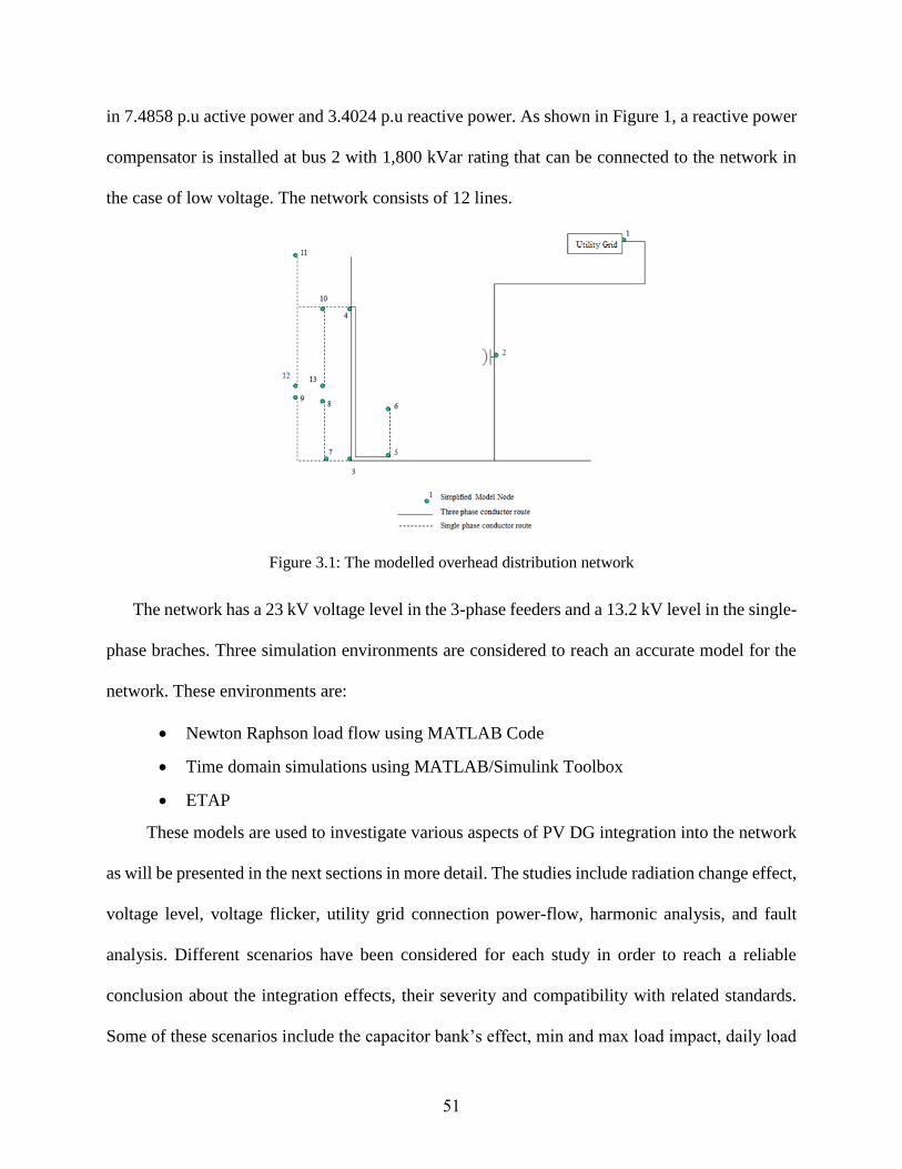
51
in 7.4858 p.u active power and 3.4024 p.u reactive power. As shown in Figure 1, a reactive power
compensator is installed at bus 2 with 1,800 kVar rating that can be connected to the network in
the case of low voltage. The network consists of 12 lines.
Figure 3.1: The modelled overhead distribution network
The network has a 23 kV voltage level in the 3-phase feeders and a 13.2 kV level in the single-
phase braches. Three simulation environments are considered to reach an accurate model for the
network. These environments are:
Newton Raphson load flow using MATLAB Code
Time domain simulations using MATLAB/Simulink Toolbox
ETAP
These models are used to investigate various aspects of PV DG integration into the network
as will be presented in the next sections in more detail. The studies include radiation change effect,
voltage level, voltage flicker, utility grid connection power-flow, harmonic analysis, and fault
analysis. Different scenarios have been considered for each study in order to reach a reliable
conclusion about the integration effects, their severity and compatibility with related standards.
Some of these scenarios include the capacitor bank’s effect, min and max load impact, daily load

52
change, daily sun radiation change and cloud impacts. For all of the cases, a recommended
maximum PV DG penetration level is determined in order to satisfy the standards.
1.14. Network’s Voltages
One of the goals in operation of the power grids is to maintain the voltages at acceptable
levels. Capacitor bank installation is the most popular compensation method for this purpose. Here,
a capacitor bank is installed on bus 2 as a means of compensation for voltage level and reactive
power support. DGs integration in the network can improve the network voltage profile. However,
any interruption in the DGs contribution, particularly when it affects a large number of them,
results in voltage fluctuations, sag, and possible flickers.
PV DGs utilized in the grid depend on solar radiation. Solar radiation changes over the 24-
hour periods. IEEE 1453, which also covers IEC 61000, and IEEE 519 definitions and limitations
for voltage quality are considered and discussed in this section. In addition, the varying solar
radiation due to passing a scattered cloud over the network area is investigated here. The solar
radiation scenarios studied are listed below:
1. Daily change in solar radiation
2. Small cloud effect
3. Large cloud effect
1.15. Solar Radiation Change
Figure 3.2 depicts the change in solar radiation during 24 hours. This solar radiation shows
the PV power generation changing from zero during the night time to 100% of the grid’s full load
at 11:00am and to the maximum power generation (150% of the full load) at 1:00pm. PV’s
maximum penetration capacity at each bus is equal to 150% of the full load installed at that bus.
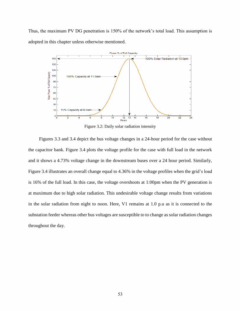
53
Thus, the maximum PV DG penetration is 150% of the network’s total load. This assumption is
adopted in this chapter unless otherwise mentioned.
Figure 3.2: Daily solar radiation intensity
Figures 3.3 and 3.4 depict the bus voltage changes in a 24-hour period for the case without
the capacitor bank. Figure 3.4 plots the voltage profile for the case with full load in the network
and it shows a 4.73% voltage change in the downstream buses over a 24 hour period. Similarly,
Figure 3.4 illustrates an overall change equal to 4.36% in the voltage profiles when the grid’s load
is 16% of the full load. In this case, the voltage overshoots at 1:00pm when the PV generation is
at maximum due to high solar radiation. This undesirable voltage change results from variations
in the solar radiation from night to noon. Here, V1 remains at 1.0 p.u as it is connected to the
substation feeder whereas other bus voltages are susceptible to to change as solar radiation changes
throughout the day.
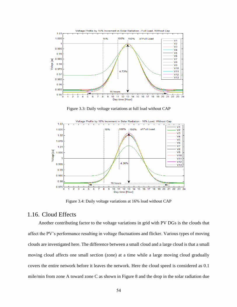
54
Figure 3.3: Daily voltage variations at full load without CAP
Figure 3.4: Daily voltage variations at 16% load without CAP
1.16. Cloud Effects
Another contributing factor to the voltage variations in grid with PV DGs is the clouds that
affect the PV’s performance resulting in voltage fluctuations and flicker. Various types of moving
clouds are investigated here. The difference between a small cloud and a large cloud is that a small
moving cloud affects one small section (zone) at a time while a large moving cloud gradually
covers the entire network before it leaves the network. Here the cloud speed is considered as 0.1
mile/min from zone A toward zone C as shown in Figure 8 and the drop in the solar radiation due
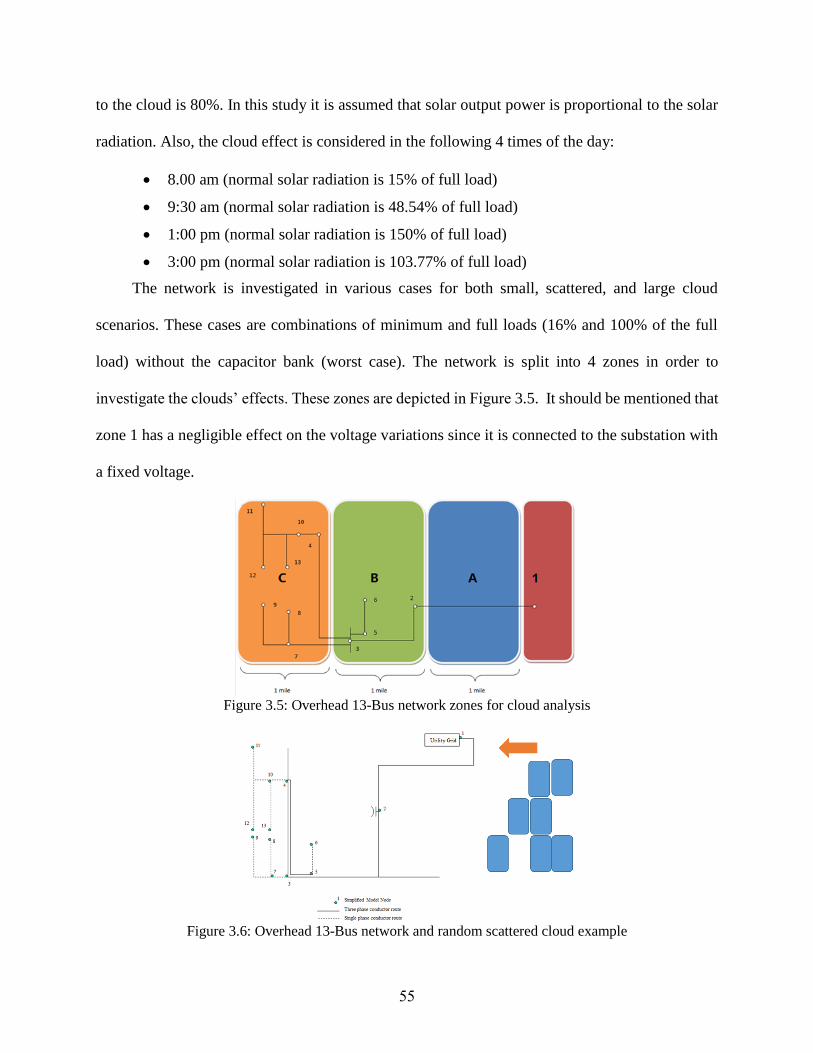
55
to the cloud is 80%. In this study it is assumed that solar output power is proportional to the solar
radiation. Also, the cloud effect is considered in the following 4 times of the day:
8.00 am (normal solar radiation is 15% of full load)
9:30 am (normal solar radiation is 48.54% of full load)
1:00 pm (normal solar radiation is 150% of full load)
3:00 pm (normal solar radiation is 103.77% of full load)
The network is investigated in various cases for both small, scattered, and large cloud
scenarios. These cases are combinations of minimum and full loads (16% and 100% of the full
load) without the capacitor bank (worst case). The network is split into 4 zones in order to
investigate the clouds’ effects. These zones are depicted in Figure 3.5. It should be mentioned that
zone 1 has a negligible effect on the voltage variations since it is connected to the substation with
a fixed voltage.
Figure 3.5: Overhead 13-Bus network zones for cloud analysis
Figure 3.6: Overhead 13-Bus network and random scattered cloud example

56
In order to investigate the cloud effects, particularly the voltage flicker, relevant standards
are considered. In general, the voltage changes fall into two categories; short term and long term
voltage variations. IEEE 1453 and IEC 61000 standards have different definitions for voltage
flicker severity evaluation based on the disturbance duration and period.
IEEE 519 has an empirical study curve made by the General Electric Company for evaluating
voltage flicker severity. It should be mentioned that companies such as Kansas City Power & Light
Company, West Pennsylvania Power Company, Detroit Edison Company, and some others have
their own empirical curves, but the GE curve is more popular and well-known. The GE curve
adopted by IEEE 519 is presented in Figure 9 and evaluates the flicker based on the frequency of
voltage change in certain periods as shown on the horizontal axis. The curve classifies flicker into
visible and irritative categories.
Note that there are three effective zones when cloud effects are studied. The small cloud is
assumed to last for 30 minutes (based on cloud speed and zone length) over each zone. Thus,
voltage fluctuation occurs three times per hour. By taking the curve of Figure 3.7 into account,
flicker limits can be considered as:
Voltage Flicker Visibility Limit: ΔV < 1%
Voltage Flicker Irritation Limit: ΔV < 3.5%
Figure 3.7: Voltage Flicker tolerance curve from IEEE 519 based on GE data
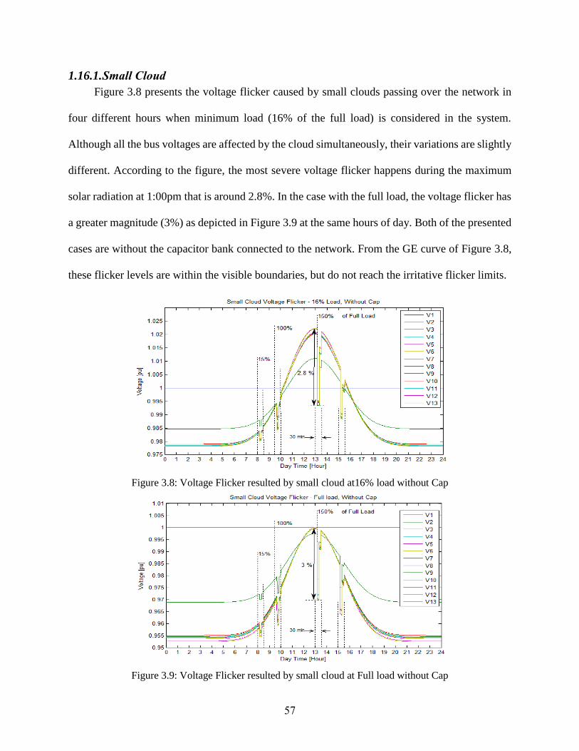
57
1.16.1. Small Cloud
Figure 3.8 presents the voltage flicker caused by small clouds passing over the network in
four different hours when minimum load (16% of the full load) is considered in the system.
Although all the bus voltages are affected by the cloud simultaneously, their variations are slightly
different. According to the figure, the most severe voltage flicker happens during the maximum
solar radiation at 1:00pm that is around 2.8%. In the case with the full load, the voltage flicker has
a greater magnitude (3%) as depicted in Figure 3.9 at the same hours of day. Both of the presented
cases are without the capacitor bank connected to the network. From the GE curve of Figure 3.8,
these flicker levels are within the visible boundaries, but do not reach the irritative flicker limits.
Figure 3.8: Voltage Flicker resulted by small cloud at16% load without Cap
Figure 3.9: Voltage Flicker resulted by small cloud at Full load without Cap
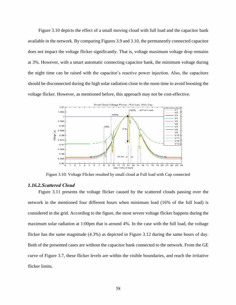
58
Figure 3.10 depicts the effect of a small moving cloud with full load and the capacitor bank
available in the network. By comparing Figures 3.9 and 3.10, the permanently connected capacitor
does not impact the voltage flicker significantly. That is, voltage maximum voltage drop remains
at 3%. However, with a smart automatic connecting capacitor bank, the minimum voltage during
the night time can be raised with the capacitor’s reactive power injection. Also, the capacitors
should be disconnected during the high solar radiation close to the noon time to avoid boosting the
voltage flicker. However, as mentioned before, this approach may not be cost-effective.
Figure 3.10: Voltage Flicker resulted by small cloud at Full load with Cap connected
1.16.2. Scattered Cloud
Figure 3.11 presents the voltage flicker caused by the scattered clouds passing over the
network in the mentioned four different hours when minimum load (16% of the full load) is
considered in the grid. According to the figure, the most severe voltage flicker happens during the
maximum solar radiation at 1:00pm that is around 4%. In the case with the full load, the voltage
flicker has the same magnitude (4.3%) as depicted in Figure 3.12 during the same hours of day.
Both of the presented cases are without the capacitor bank connected to the network. From the GE
curve of Figure 3.7, these flicker levels are within the visible boundaries, and reach the irritative
flicker limits.
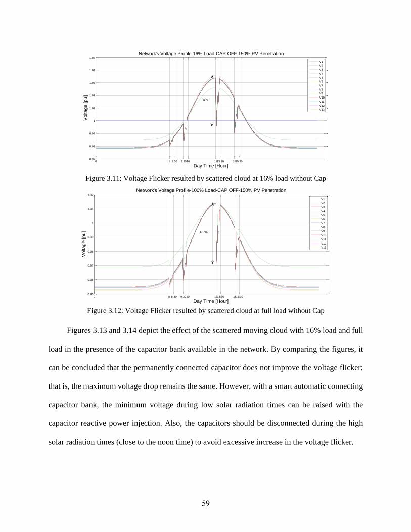
59
Figure 3.11: Voltage Flicker resulted by scattered cloud at 16% load without Cap
Figure 3.12: Voltage Flicker resulted by scattered cloud at full load without Cap
Figures 3.13 and 3.14 depict the effect of the scattered moving cloud with 16% load and full
load in the presence of the capacitor bank available in the network. By comparing the figures, it
can be concluded that the permanently connected capacitor does not improve the voltage flicker;
that is, the maximum voltage drop remains the same. However, with a smart automatic connecting
capacitor bank, the minimum voltage during low solar radiation times can be raised with the
capacitor reactive power injection. Also, the capacitors should be disconnected during the high
solar radiation times (close to the noon time) to avoid excessive increase in the voltage flicker.
0 8 8:30 9:3010 1313:30 1515:300.97
0.98
0.99
1
1.01
1.02
1.03
1.04
1.05
Network's Voltage Profile-16% Load-CAP OFF-150% PV Penetration
Day Time [Hour]
Voltage [pu]
V1
V2
V3
V4
V5
V6
V7
V8
V9
V10
V11
V12
V13
4%
0 8 8:30 9:3010 1313:30 1515:300.95
0.96
0.97
0.98
0.99
1
1.01
1.02
Network's Voltage Profile-100% Load-CAP OFF-150% PV Penetration
Day Time [Hour]
Voltage [pu]
V1
V2
V3
V4
V5
V6
V7
V8
V9
V10
V11
V12
V13
4.3%
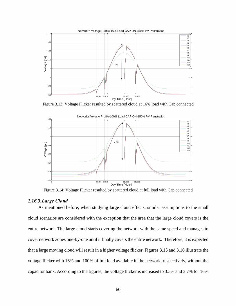
60
Figure 3.13: Voltage Flicker resulted by scattered cloud at 16% load with Cap connected
Figure 3.14: Voltage Flicker resulted by scattered cloud at full load with Cap connected
1.16.3. Large Cloud
As mentioned before, when studying large cloud effects, similar assumptions to the small
cloud scenarios are considered with the exception that the area that the large cloud covers is the
entire network. The large cloud starts covering the network with the same speed and manages to
cover network zones one-by-one until it finally covers the entire network. Therefore, it is expected
that a large moving cloud will result in a higher voltage flicker. Figures 3.15 and 3.16 illustrate the
voltage flicker with 16% and 100% of full load available in the network, respectively, without the
capacitor bank. According to the figures, the voltage flicker is increased to 3.5% and 3.7% for 16%
0 8 8:30 9:3010 1313:30 1515:300.98
0.99
1
1.01
1.02
1.03
1.04
1.05
Network's Voltage Profile-16% Load-CAP ON-150% PV Penetration
Day Time [Hour]
Voltage [pu]
V1
V2
V3
V4
V5
V6
V7
V8
V9
V10
V11
V12
V134%
0 8 8:30 9:3010 1313:30 1515:300.95
0.96
0.97
0.98
0.99
1
1.01
1.02
Network's Voltage Profile-100% Load-CAP ON-150% PV Penetration
Day Time [Hour]
Voltage [pu]
V1
V2
V3
V4
V5
V6
V7
V8
V9
V10
V11
V12
V13
4.3%
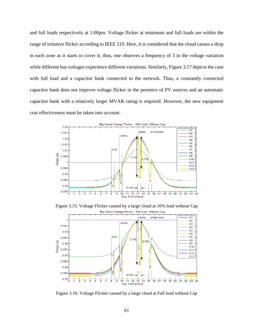
61
and full loads respectively at 1:00pm. Voltage flicker at minimum and full loads are within the
range of irritative flicker according to IEEE 519. Here, it is considered that the cloud causes a drop
in each zone as it starts to cover it; thus, one observes a frequency of 3 in the voltage variation
while different bus voltages experience different variations. Similarly, Figure 3.17 depicts the case
with full load and a capacitor bank connected to the network. Thus, a constantly connected
capacitor bank does not improve voltage flicker in the presence of PV sources and an automatic
capacitor bank with a relatively larger MVAR rating is required. However, the new equipment
cost effectiveness must be taken into account.
Figure 3.15: Voltage Flicker caused by a large cloud at 16% load without Cap
Figure 3.16: Voltage Flicker caused by a large cloud at Full load without Cap
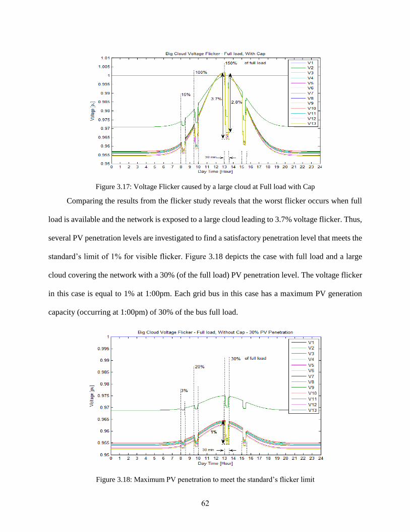
62
Figure 3.17: Voltage Flicker caused by a large cloud at Full load with Cap
Comparing the results from the flicker study reveals that the worst flicker occurs when full
load is available and the network is exposed to a large cloud leading to 3.7% voltage flicker. Thus,
several PV penetration levels are investigated to find a satisfactory penetration level that meets the
standard’s limit of 1% for visible flicker. Figure 3.18 depicts the case with full load and a large
cloud covering the network with a 30% (of the full load) PV penetration level. The voltage flicker
in this case is equal to 1% at 1:00pm. Each grid bus in this case has a maximum PV generation
capacity (occurring at 1:00pm) of 30% of the bus full load.
Figure 3.18: Maximum PV penetration to meet the standard’s flicker limit

63
1.17. Reactive Power Compensation
Reactive power compensation is an important and usually necessary approach for power
networks especially those with PV integration. Both connected and islanded modes are simulated
here. Two scenarios are considered for islanded mode operation:
1. PV active power > Full load + Losses : Abundant PV active Power
The PV total active power generation is more than the network’s demand (i.e., the loads
consumptions and power losses)
2. PV active power < Full load + Losses : Shortage in PV active Power
The PV total active power generation is less than the network consumption. These situations are
summarized below:
1.17.1. Scenario 1: Connected Mode
For proper compensation, a capacitor bank has been installed on bus 3 with size roughly 4
times bigger than original system CAP, i.e. 1.4 p.u. The capacitor compensation results in a voltage
shift in all buses which may lead into excessive voltage at noon time due to PV power. An
automatically tapped capacitor compensation has been evaluated which results in less over voltage
during 24 hours. Figures 3.19 and 3.20 represent the voltage profiles for the cases with 100% load
in the network without and with the CAP, respectively. Installing a permanently fully connected
1.4 p.u. capacitor on bus 3 results in a noticeable shift in voltage profile.
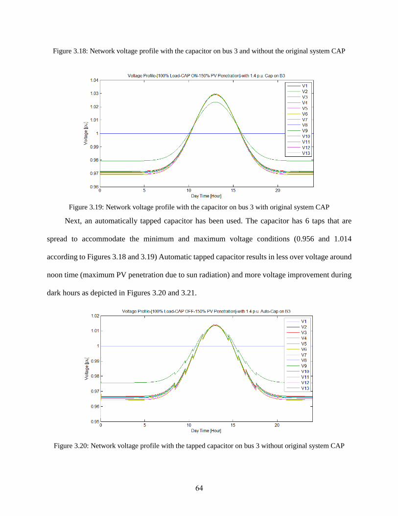
64
Figure 3.18: Network voltage profile with the capacitor on bus 3 and without the original system CAP
Figure 3.19: Network voltage profile with the capacitor on bus 3 with original system CAP
Next, an automatically tapped capacitor has been used. The capacitor has 6 taps that are
spread to accommodate the minimum and maximum voltage conditions (0.956 and 1.014
according to Figures 3.18 and 3.19) Automatic tapped capacitor results in less over voltage around
noon time (maximum PV penetration due to sun radiation) and more voltage improvement during
dark hours as depicted in Figures 3.20 and 3.21.
Figure 3.20: Network voltage profile with the tapped capacitor on bus 3 without original system CAP
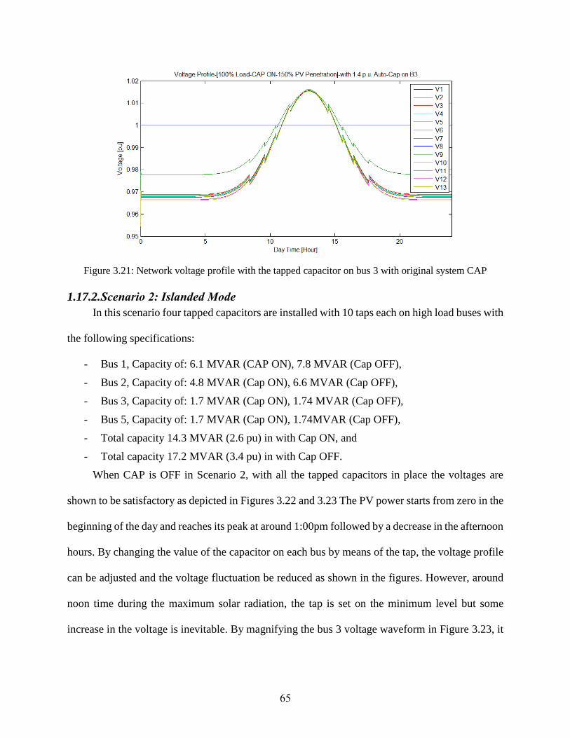
65
Figure 3.21: Network voltage profile with the tapped capacitor on bus 3 with original system CAP
1.17.2. Scenario 2: Islanded Mode
In this scenario four tapped capacitors are installed with 10 taps each on high load buses with
the following specifications:
- Bus 1, Capacity of: 6.1 MVAR (CAP ON), 7.8 MVAR (Cap OFF),
- Bus 2, Capacity of: 4.8 MVAR (Cap ON), 6.6 MVAR (Cap OFF),
- Bus 3, Capacity of: 1.7 MVAR (Cap ON), 1.74 MVAR (Cap OFF),
- Bus 5, Capacity of: 1.7 MVAR (Cap ON), 1.74MVAR (Cap OFF),
- Total capacity 14.3 MVAR (2.6 pu) in with Cap ON, and
- Total capacity 17.2 MVAR (3.4 pu) in with Cap OFF.
When CAP is OFF in Scenario 2, with all the tapped capacitors in place the voltages are
shown to be satisfactory as depicted in Figures 3.22 and 3.23 The PV power starts from zero in the
beginning of the day and reaches its peak at around 1:00pm followed by a decrease in the afternoon
hours. By changing the value of the capacitor on each bus by means of the tap, the voltage profile
can be adjusted and the voltage fluctuation be reduced as shown in the figures. However, around
noon time during the maximum solar radiation, the tap is set on the minimum level but some
increase in the voltage is inevitable. By magnifying the bus 3 voltage waveform in Figure 3.23, it
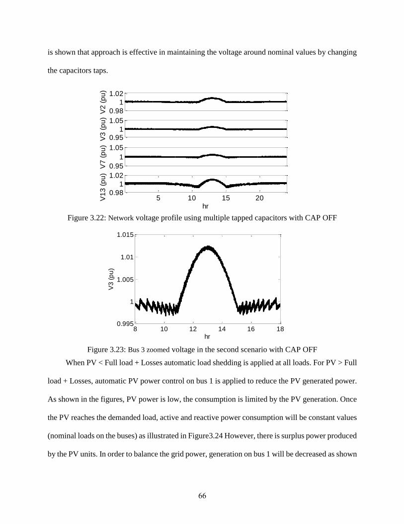
66
is shown that approach is effective in maintaining the voltage around nominal values by changing
the capacitors taps.
Figure 3.22: Network voltage profile using multiple tapped capacitors with CAP OFF
Figure 3.23: Bus 3 zoomed voltage in the second scenario with CAP OFF
When PV < Full load + Losses automatic load shedding is applied at all loads. For PV > Full
load + Losses, automatic PV power control on bus 1 is applied to reduce the PV generated power.
As shown in the figures, PV power is low, the consumption is limited by the PV generation. Once
the PV reaches the demanded load, active and reactive power consumption will be constant values
(nominal loads on the buses) as illustrated in Figure3.24 However, there is surplus power produced
by the PV units. In order to balance the grid power, generation on bus 1 will be decreased as shown
0.98
1
1.02
V2
(p
u)
0.951
1.05
V3
(p
u)
0.95
1
1.05
V7
(p
u)
5 10 15 200.98
1
1.02
hr
V1
3 (
pu
)
8 10 12 14 16 180.995
1
1.005
1.01
1.015
hr
V3
(p
u)
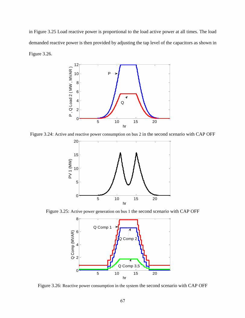
67
in Figure 3.25 Load reactive power is proportional to the load active power at all times. The load
demanded reactive power is then provided by adjusting the tap level of the capacitors as shown in
Figure 3.26.
Figure 3.24: Active and reactive power consumption on bus 2 in the second scenario with CAP OFF
Figure 3.25: Active power generation on bus 1 the second scenario with CAP OFF
Figure 3.26: Reactive power consumption in the system the second scenario with CAP OFF
5 10 15 200
2
4
6
8
10
12
hr
P , Q
Lo
ad
2 (
MW
, M
VA
R )
P
Q
5 10 15 200
5
10
15
20
hr
PV
1 (
MW
)
5 10 15 200
2
4
6
8
hr
Q C
om
p (
MV
AR
)
Q Comp 1
Q Comp 2
Q Comp 3,5

68
1.18. Fault Current Level
DGs integration may have critical influences on fault situations and the protection system.
IEEE standards mention that inverter interfaced DGs should have a limited fault current to be no
more than twice that of their normal current for limited duration for protecting their switching
devices. However, this amount of current can affect the fault current magnitude in the network.
This change in fault current characteristics may have significant effects on the protection system
such as delayed trip, miscoordination, or blinding.
A fault study has been performed here by simulating a fault in highly loaded buses of the
network with a focus on the utility grid protection system. That is, buses 2,3,5,7, and 10 are
analyzed for fault scenarios in cases with full load and 16% of the load. It is assumed that the
pickup settings for the utility grid relays are twice their normal currents during the full load
working condition, (i.e., two times 7.77 p.u or 15.54 p.u.). Faults are simulated as high power loads
(high impedance faults.)
Figure 3.27 depicts the utility grid and the sum of the PV DG contribution in a 3-phase fault
at bus 2 with full load available in the network. The time axis indicates the hour in which the fault
occurs. As shown in Figure 3.27, when the fault happens at night i.e., zero PVs contribution, all
the fault current (approximately equal to 24.5 p.u) is injected by the utility grid. This current is
more than the utility grid’s protection threshold and is easy to detect. However, when the PV
penetration exceeds 124% (of the full load, based on sun radiation) the utility grid contribution to
the fault current will be less than its protection threshold as shown in the figure. The PV
contribution to the fault current significantly reduces the utility grid’s contribution. Such a fault,
in this case, cannot be diagnosed and tripped by the utility grid’s protective system (blinding
phenomenon.)
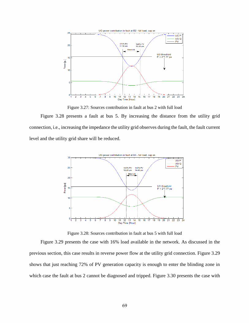
69
Figure 3.27: Sources contribution in fault at bus 2 with full load
Figure 3.28 presents a fault at bus 5. By increasing the distance from the utility grid
connection, i.e., increasing the impedance the utility grid observes during the fault, the fault current
level and the utility grid share will be reduced.
Figure 3.28: Sources contribution in fault at bus 5 with full load
Figure 3.29 presents the case with 16% load available in the network. As discussed in the
previous section, this case results in reverse power flow at the utility grid connection. Figure 3.29
shows that just reaching 72% of PV generation capacity is enough to enter the blinding zone in
which case the fault at bus 2 cannot be diagnosed and tripped. Figure 3.30 presents the case with
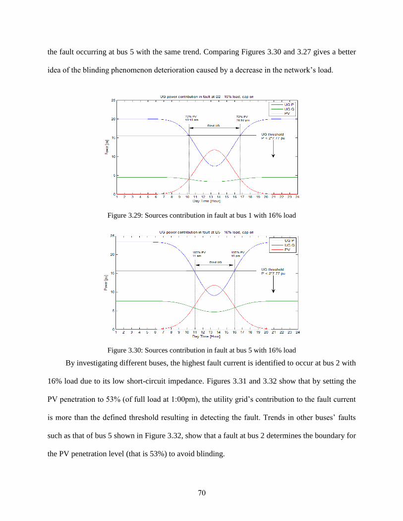
70
the fault occurring at bus 5 with the same trend. Comparing Figures 3.30 and 3.27 gives a better
idea of the blinding phenomenon deterioration caused by a decrease in the network’s load.
Figure 3.29: Sources contribution in fault at bus 1 with 16% load
Figure 3.30: Sources contribution in fault at bus 5 with 16% load
By investigating different buses, the highest fault current is identified to occur at bus 2 with
16% load due to its low short-circuit impedance. Figures 3.31 and 3.32 show that by setting the
PV penetration to 53% (of full load at 1:00pm), the utility grid’s contribution to the fault current
is more than the defined threshold resulting in detecting the fault. Trends in other buses’ faults
such as that of bus 5 shown in Figure 3.32, show that a fault at bus 2 determines the boundary for
the PV penetration level (that is 53%) to avoid blinding.
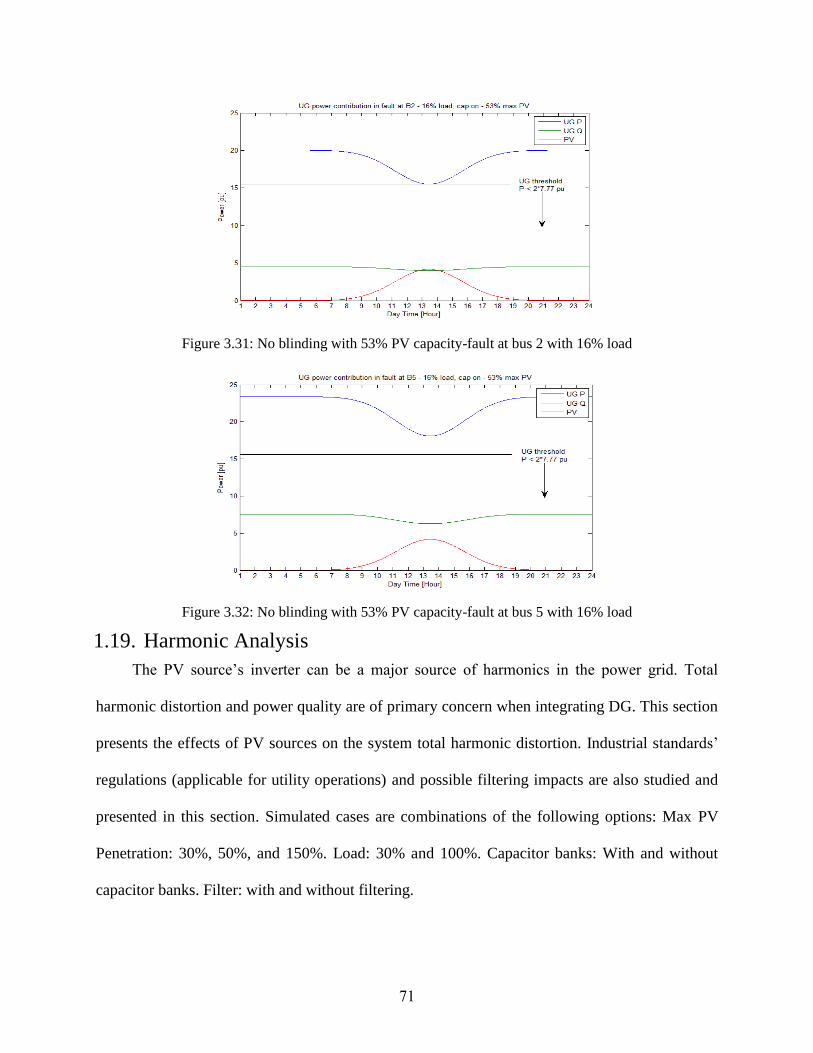
71
Figure 3.31: No blinding with 53% PV capacity-fault at bus 2 with 16% load
Figure 3.32: No blinding with 53% PV capacity-fault at bus 5 with 16% load
1.19. Harmonic Analysis
The PV source’s inverter can be a major source of harmonics in the power grid. Total
harmonic distortion and power quality are of primary concern when integrating DG. This section
presents the effects of PV sources on the system total harmonic distortion. Industrial standards’
regulations (applicable for utility operations) and possible filtering impacts are also studied and
presented in this section. Simulated cases are combinations of the following options: Max PV
Penetration: 30%, 50%, and 150%. Load: 30% and 100%. Capacitor banks: With and without
capacitor banks. Filter: with and without filtering.
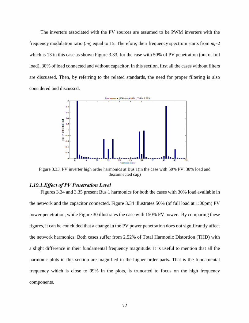
72
The inverters associated with the PV sources are assumed to be PWM inverters with the
frequency modulation ratio (mf) equal to 15. Therefore, their frequency spectrum starts from mf -2
which is 13 in this case as shown Figure 3.33, for the case with 50% of PV penetration (out of full
load), 30% of load connected and without capacitor. In this section, first all the cases without filters
are discussed. Then, by referring to the related standards, the need for proper filtering is also
considered and discussed.
Figure 3.33: PV inverter high order harmonics at Bus 1(in the case with 50% PV, 30% load and
disconnected cap)
1.19.1. Effect of PV Penetration Level
Figures 3.34 and 3.35 present Bus 1 harmonics for both the cases with 30% load available in
the network and the capacitor connected. Figure 3.34 illustrates 50% (of full load at 1:00pm) PV
power penetration, while Figure 30 illustrates the case with 150% PV power. By comparing these
figures, it can be concluded that a change in the PV power penetration does not significantly affect
the network harmonics. Both cases suffer from 2.52% of Total Harmonic Distortion (THD) with
a slight difference in their fundamental frequency magnitude. It is useful to mention that all the
harmonic plots in this section are magnified in the higher order parts. That is the fundamental
frequency which is close to 99% in the plots, is truncated to focus on the high frequency
components.
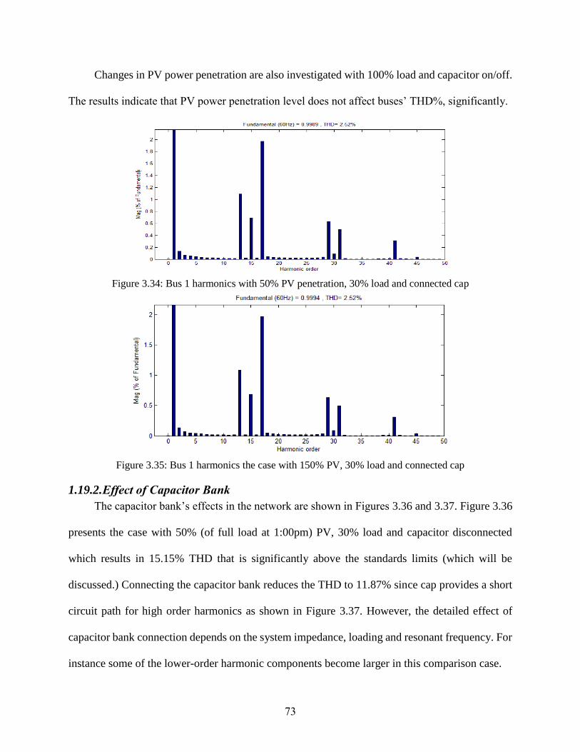
73
Changes in PV power penetration are also investigated with 100% load and capacitor on/off.
The results indicate that PV power penetration level does not affect buses’ THD%, significantly.
Figure 3.34: Bus 1 harmonics with 50% PV penetration, 30% load and connected cap
Figure 3.35: Bus 1 harmonics the case with 150% PV, 30% load and connected cap
1.19.2. Effect of Capacitor Bank
The capacitor bank’s effects in the network are shown in Figures 3.36 and 3.37. Figure 3.36
presents the case with 50% (of full load at 1:00pm) PV, 30% load and capacitor disconnected
which results in 15.15% THD that is significantly above the standards limits (which will be
discussed.) Connecting the capacitor bank reduces the THD to 11.87% since cap provides a short
circuit path for high order harmonics as shown in Figure 3.37. However, the detailed effect of
capacitor bank connection depends on the system impedance, loading and resonant frequency. For
instance some of the lower-order harmonic components become larger in this comparison case.
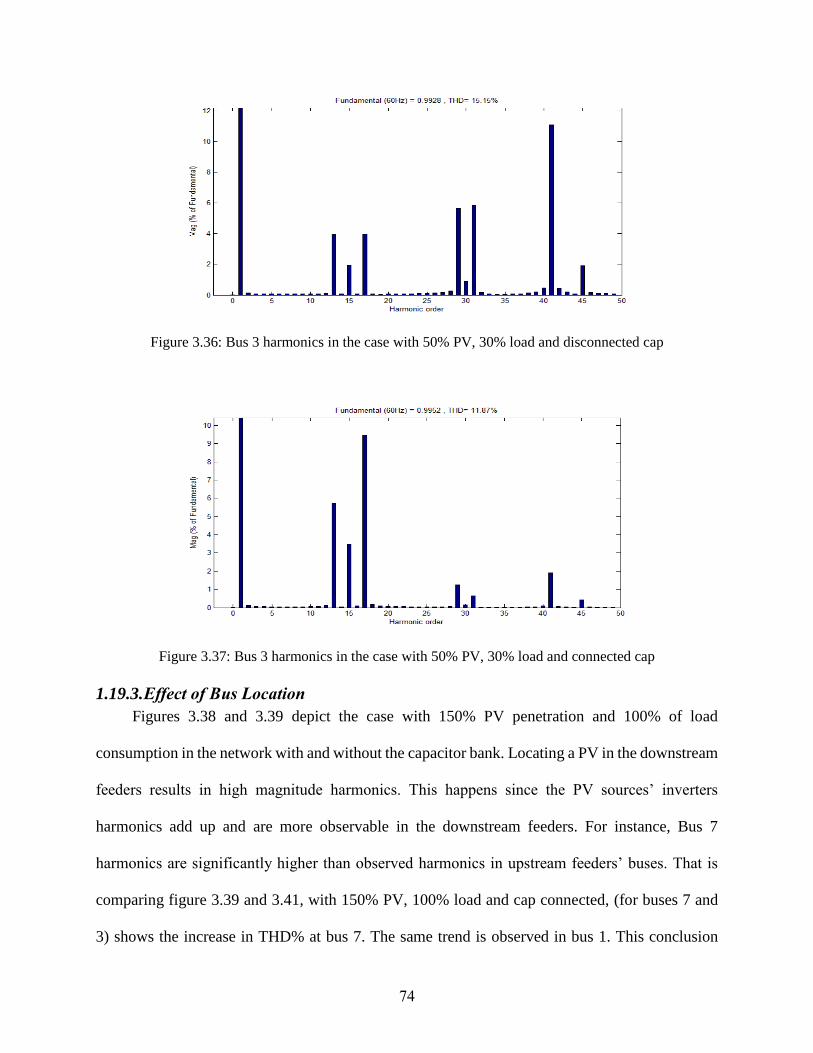
74
Figure 3.36: Bus 3 harmonics in the case with 50% PV, 30% load and disconnected cap
Figure 3.37: Bus 3 harmonics in the case with 50% PV, 30% load and connected cap
1.19.3. Effect of Bus Location
Figures 3.38 and 3.39 depict the case with 150% PV penetration and 100% of load
consumption in the network with and without the capacitor bank. Locating a PV in the downstream
feeders results in high magnitude harmonics. This happens since the PV sources’ inverters
harmonics add up and are more observable in the downstream feeders. For instance, Bus 7
harmonics are significantly higher than observed harmonics in upstream feeders’ buses. That is
comparing figure 3.39 and 3.41, with 150% PV, 100% load and cap connected, (for buses 7 and
3) shows the increase in THD% at bus 7. The same trend is observed in bus 1. This conclusion
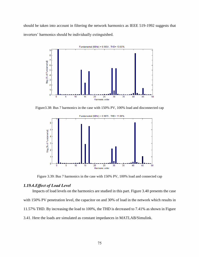
75
should be taken into account in filtering the network harmonics as IEEE 519-1992 suggests that
inverters’ harmonics should be individually extinguished.
Figure3.38: Bus 7 harmonics in the case with 150% PV, 100% load and disconnected cap
Figure 3.39: Bus 7 harmonics in the case with 150% PV, 100% load and connected cap
1.19.4. Effect of Load Level
Impacts of load levels on the harmonics are studied in this part. Figure 3.40 presents the case
with 150% PV penetration level, the capacitor on and 30% of load in the network which results in
11.57% THD. By increasing the load to 100%, the THD is decreased to 7.41% as shown in Figure
3.41. Here the loads are simulated as constant impedances in MATLAB/Simulink.
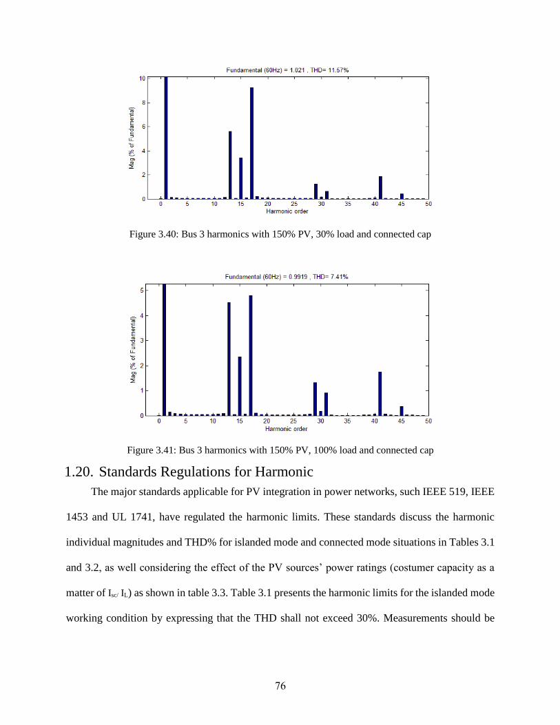
76
Figure 3.40: Bus 3 harmonics with 150% PV, 30% load and connected cap
Figure 3.41: Bus 3 harmonics with 150% PV, 100% load and connected cap
1.20. Standards Regulations for Harmonic
The major standards applicable for PV integration in power networks, such IEEE 519, IEEE
1453 and UL 1741, have regulated the harmonic limits. These standards discuss the harmonic
individual magnitudes and THD% for islanded mode and connected mode situations in Tables 3.1
and 3.2, as well considering the effect of the PV sources’ power ratings (costumer capacity as a
matter of Isc/ IL) as shown in table 3.3. Table 3.1 presents the harmonic limits for the islanded mode
working condition by expressing that the THD shall not exceed 30%. Measurements should be
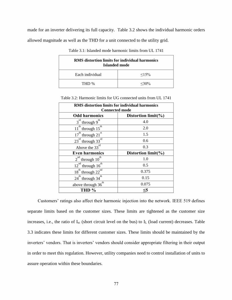
77
made for an inverter delivering its full capacity. Table 3.2 shows the individual harmonic orders
allowed magnitude as well as the THD for a unit connected to the utility grid.
Table 3.1: Islanded mode harmonic limits from UL 1741
RMS distortion limits for individual harmonics
Islanded mode
Each individual ≤15%
THD % ≤30%
Table 3.2: Harmonic limits for UG connected units from UL 1741
RMS distortion limits for individual harmonics
Connected mode
Odd harmonics Distortion limit(%)
3rd
through 9th 4.0
11th through 15
th 2.0
17th through 21
st 1.5
23rd
through 33rd
0.6
Above the 33rd
0.3
Even harmonics Distortion limit(%)
2nd
through 10th 1.0
12nd
through 16th 0.5
18th through 22
nd 0.375
24th through 34
th 0.15
above through 36th 0.075
THD % ≤5
Customers’ ratings also affect their harmonic injection into the network. IEEE 519 defines
separate limits based on the customer sizes. These limits are tightened as the customer size
increases, i.e., the ratio of Isc (short circuit level on the bus) to IL (load current) decreases. Table
3.3 indicates these limits for different customer sizes. These limits should be maintained by the
inverters’ vendors. That is inverters’ vendors should consider appropriate filtering in their output
in order to meet this regulation. However, utility companies need to control installation of units to
assure operation within these boundaries.

78
Table 3.3: Distortion limits based on customer size from IEEE 519
Maximum Harmonic Distortion in Percent of IL
Individual Harmonic Orders (Odd harmonics)
Isc/ IL <11 11≤h<17 17≤h<23 23≤h<35 35≤h THD%
< 20* 4.0 2.0 1.5 0.6 0.3 5.0
20<50 7.0 3.5 2.5 1.0 0.5 8.0
50<100 10.0 4.5 4.0 1.5 0.7 12.0
100<1000 12.0 5.5 5.0 2.0 1.0 15.0
>1000 15.0 7.0 6.0 2.5 1.4 20.0
Even harmonics are limited to 25% of odd harmonic limits above.
Current distortion that results in dc offset, e.g. half wave converters, are not
allowed.
* All power generation equipment is limited to these values of current distortion
regardless of Isc/ IL ratio.
Where
Isc = Maximum short circuit current at PCC.
IL = Maximum demand load current (fundamental frequency component at PCC)
1.21. Filtering effect on Harmonic
As discussed previously, the PV source’s inverter harmonic spectrum starts at higher orders.
Therefore, a low pass filter is the most suitable approach for reducing the harmonics. This section
presents the significant impacts that harmonic filters have on harmonic reduction. In the following
simulations filters have been installed in the output of each PV unit. Figure 3.42 presents the
harmonic spectrum for the case with 50% PV, 30% load, and capacitor disconnected. The THD at
Bus 1 is reduced from 2.52% to 0.63% as compared to Figure 3.33, i.e., the same case with 50%
PV, 30% load and disconnected cap but without filters. It should be mentioned that before filtering
the actual case did not meet the standards’ regulations, whereas these limits are met by including
the filters. A similar trend happens in other cases, too.
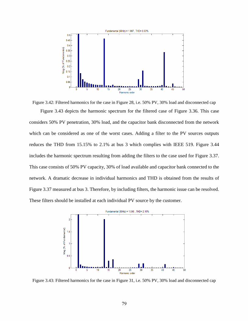
79
Figure 3.42: Filtered harmonics for the case in Figure 28, i.e. 50% PV, 30% load and disconnected cap
Figure 3.43 depicts the harmonic spectrum for the filtered case of Figure 3.36. This case
considers 50% PV penetration, 30% load, and the capacitor bank disconnected from the network
which can be considered as one of the worst cases. Adding a filter to the PV sources outputs
reduces the THD from 15.15% to 2.1% at bus 3 which complies with IEEE 519. Figure 3.44
includes the harmonic spectrum resulting from adding the filters to the case used for Figure 3.37.
This case consists of 50% PV capacity, 30% of load available and capacitor bank connected to the
network. A dramatic decrease in individual harmonics and THD is obtained from the results of
Figure 3.37 measured at bus 3. Therefore, by including filters, the harmonic issue can be resolved.
These filters should be installed at each individual PV source by the customer.
Figure 3.43: Filtered harmonics for the case in Figure 31, i.e. 50% PV, 30% load and disconnected cap
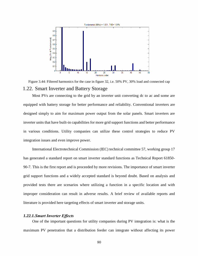
80
Figure 3.44: Filtered harmonics for the case in figure 32, i.e. 50% PV, 30% load and connected cap
1.22. Smart Inverter and Battery Storage
Most PVs are connecting to the grid by an inverter unit converting dc to ac and some are
equipped with battery storage for better performance and reliability. Conventional inverters are
designed simply to aim for maximum power output from the solar panels. Smart inverters are
inverter units that have built-in capabilities for more grid support functions and better performance
in various conditions. Utility companies can utilize these control strategies to reduce PV
integration issues and even improve power.
International Electrotechnical Commission (IEC) technical committee 57, working group 17
has generated a standard report on smart inverter standard functions as Technical Report 61850-
90-7. This is the first report and is proceeded by more revisions. The importance of smart inverter
grid support functions and a widely accepted standard is beyond doubt. Based on analysis and
provided tests there are scenarios where utilizing a function in a specific location and with
improper consideration can result in adverse results. A brief review of available reports and
literature is provided here targeting effects of smart inverter and storage units.
1.22.1. Smart Inverter Effects
One of the important questions for utility companies during PV integration is: what is the
maximum PV penetration that a distribution feeder can integrate without affecting its power

81
quality or reliability; that is, the feeder hosting capacity determining the maximum possible PV
penetration. Smart inverters’ functions can improve PV integration issues if employed properly.
Studies show that an improper usage of such function can result in adverse impacts. Three
functions are discussed in this section which are widely accepted and the most effective for
increasing distribution feeders hosting capacity. These functions include:
Fixed Power factor
Volt-VAR
Volt-Watt
Function Effects: Fixed power factor
Using this function, smart inverter can absorb the excessive reactive power from the network
and consequently reduce the overvoltage effect resulted by extra active power injection.
− PV units can cause overvoltage due to excessive injection of active power
− A fixed power factor improves the excess voltage level by absorbing reactive power
from the network by the inverter
− Fixed PF and amount of reactive power absorption is highly dependent on the feeder
X/R ratio
− In general, a set PF to 0.85 to 0.98 is common, PF equal to 0.95 to 0.98 seems effective
for feeders with X/R ratio between 3 to 5,
− In general, a lower fixed PF has greater improvement effect on a feeder hosting capacity,
especially for feeders that already have voltage issues
− Fixed PF function cannot fix the preexisting voltage issue on a feeder
− Depending on the overall feeder load PF, it is possible that using a low fixed PF cause
under-voltage in a feeder
− Fixed power factor significantly increases the maximum hosting capacity on distribution
feeders
Function Effects: Volt-VAR
The function provides more adaptive VAR control responding to the DERs PCC voltage.
Utility or owner can set the function using the function curve.
− Volt-VAR control mostly results in increasing minimum and maximum hosting capacity
but neutral and adverse effects are possible
− The function can have interference with voltage regulators causing adverse effect

82
− Volt-VAR tries to maintain voltage close to nominal causing extra reactive power flow
− The function can cause voltage drop in upstream voltage regulators
− The function without dead-band seems to have better impacts on hosting capacity
− Proper settings considering the feeder existing operational details is important
− Detailed case analysis before applying the function is advised
− Volt-VAR function provides better improvement on voltage levels in feeders with pre-
existing voltage issues
− Available reactive power capacity is important in the performance of the function
Function Effects: Volt-Watt
This function also provides an adaptive mechanism where the unit’s active power can be
regulated based on the measured voltage.
− Volt-Watt function increases hosting capacity in most observations
− Neutral effect on hosting capacity is observed in few cases but no adverse results yet
− The function has not shown improvement in pre-existing voltage issues in feeders
− Higher settings (high voltage threshold for active power curtailment initiation) has no
significant effects on hosting capacity
Parallel Operation
Smart inverter parallel operation can cause unexpected effects where possible interferences
between different grid support functions are possible. Ongoing research is still working on
discovering various aspects of the smart inverter parallel operation.
1.22.2. Battery Storage
Various types of storage technologies are considered and still under test and development
for power storage with each having their own specifications and limitations. In general, battery
storage challenges can be categorized under three main topics that are,
Battery technology
Storage unit control algorithm
Project management and logistics
Technical effects and conclusions
− Voltage regulation with PV units using storage within ANSI limits is achieved both in
study and practice

83
− Reducing the maximum voltage level and improving the minimum voltage with high
PV penetration is an objective of storage units deployment
− Best results are obtained with bigger storage sizes closer to the end of the feeder
− Peak shaving and Load shifting have not shown a noticeable effect on voltage level for
the studied networks, in some cases adverse effects are observed
− Storage unit proper design results in lower power losses in the network
− Using storage unit, a preferred load curve for feeder or substation is achievable
− Applications of storage can be costly, but with proper design and sizing it’s a viable
solution even for responding to frequency variations
− Using battery storage units with smoothing and defined load curve capabilities can
reduce the number of tap changes in half for a nearby substation
− Utilizing hybrid battery storage (using different types of batteries) results in a wider
variety of applications; i.e., high power battery provides voltage support and PV output
smoothing whereas high energy battery enables peak shaving and time shifting
− Grid-tied battery storage unit projects focuses are shifted from technical challenges to
economic optimization; algorithms for this aim are still under development
− A business model tailored for customer-owned energy storage systems is needed
− Currently available day-ahead weather models are not dependable or accurate for
storage units curve determination
− Fault current changes during islanded operation requires specific protections design
− An auxiliary power should be considered for microgrids that are designed to operate in
islanded mode for voltage regulation in the presence of inverters (constant voltage
transformer is a solution with high expense)
1.23. References
[1] IEEE Recommended Practices and Requirements for Harmonic Control in Electrical
Power Systems," IEEE Std 519-1992 , vol., no., pp.1,112, April 9 1993
[2] IEEE Recommended Practice for Utility Interface of Photovoltaic (PV) Systems," IEEE
Std 929-2000 , vol., no., pp.i,, 2000
[3] IEEE Recommended Practice--Adoption of IEC 61000-4-15:2010, Electromagnetic
compatibility (EMC)--Testing and measurement techniques--Flickermeter--Functional and
design specifications," IEEE Std 1453-2011 , vol., no., pp.1,58, Oct. 21 2011
[4] IEEE Application Guide for IEEE Std 1547, IEEE Standard for Interconnecting Distributed
Resources with Electric Power Systems," IEEE Std 1547.2-2008 , vol., no., pp.1,207,
April 15 2009
[5] UL 1741 standard on Inverters, Converters, Controllers and Interconnection System
Equipment for Use With Distributed Energy Resources
84
[6] Common Functions for Smart Inverters, Version 3. EPRI, Palo Alto, CA: 2013.
3002002233
[7] Grid Impacts of Distributed Generation with Advanced Inverter Functions: Hosting
Capacity of Large-Scale Solar Photovoltaic Using Smart Inverters. EPRI, Palo Alto, CA:
2013. 3002001246
[8] Application Guid for Integration of Grid-Supportive Inverters: Version 1. EPRI, Palo Alto,
CA: 2013. 3002001248
[9] Distribution Management Systems and Advanced Inverters: Autonomous Versus
Integrated PV Control. EPRI, Palo Alto, CA: 2014. 3002003275
[10] Smart Inverter Field Experiences: A State of the Industry Overview. EPRI, Palo
Alto, CA: 2013. 3002001247
[11] Recommended Smart Inverter Settings: Power Factor Control. EPRI, Palo Alto,
CA: 2014. 3002003274
[12] Parallel Operation of Multiple Smart Inverters. EPRI, Palo Alto, CA: 2015.
3002005784
[13] Evaluation of Three-Phase Photovoltaic Inverters with Grid Support Functionality.
EPRI, Palo Alto, CA: 2012. 1024361
[14] Modeling of a Battery Storage System for Southern Co: Application of Smart
Inverter Functions for Energy Storage in OpenDSS. EPRI, Palo Alto, CA: 2016.
3002007481
[15] Analysis of Distribution System Effects of Energy Storage Through Simulation and
Modelling: Energy Storage Grid Integration Analysis with OpenDSS. EPRI, Palo Alto,
CA: 2012. 1024285
[16] Case Studies Evaluating Energy Storage as an Effective Grid Integration Tool:
Selected Worldwide Results, Findings, and Lessons Learned. EPRI, Palo Alto, CA: 2014.
3002003271
[17] Utilizing Energy Storage as a PV Grid Integration Tool: Utility project case studies.
EPRI, Palo Alto, CA: 2015. 3002005780
[18] Laboratory Evaluation of Grid-Tied Photovoltaic and Energy Storage Systems,
EPRI, Palo Alto, CA: 2011. 1021987
[19] The Solar-to-Battery and Community Energy Storage Project
Demonstrations at the Solar Energy Acceleration Center, 2015 Test Results and Analysis,
EPRI, Palo Alto, CA: 2015.3002005786
85
Chapter 4
Challenges of PV Integration in Low-Voltage
Secondary (Downtown) Networks
1.24. Introduction
Electric power systems have been experiencing fast and fundamental changes in recent years
due to the introduction of distributed generation (DG). The smart grid, utilizing renewable energy-
based distributed generation, attracts great attention due to environmental and reliability concerns
[1], [2]. Government incentives, technological advances, and many other factors have resulted in
a dramatic growth in photovoltaic (PV) power utilization and integration by both customers and
utility companies [1]–[3]. Approximately 1.3 gigawatts of PV power were installed in the United
States in the first quarter of 2015 resulting in a total of 21.3 GW of installed capacity [3]. The
residential share of this installed capacity is 400 megawatts, which is a 76% rise compared to the
same period in 2014 [3]. While this rapid pace of PV integration can potentially cause problems if
not treated properly, both the government and utility customers have a great desire for PV
integration.
Conventional urban lateral distribution networks are designed to accommodate unidirectional
power flow from generation plants to the customers. This assumption is prone to violation by PV
units causing reverse power flow in the case of excess power generation. The bidirectional flow of
power can potentially interfere with the protective equipment. Other network operational
conditions such as voltage profile, flicker, etc., can also be affected by the presence of PV power
[1], [2]. Cloud effect, weather unpredictability, sun irradiance hourly changes, uncertainties in PV
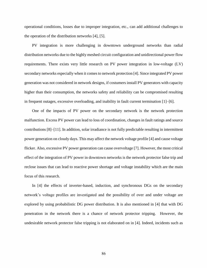
86
operational conditions, losses due to improper integration, etc., can add additional challenges to
the operation of the distribution networks [4], [5].
PV integration is more challenging in downtown underground networks than radial
distribution networks due to the highly meshed circuit configuration and unidirectional power flow
requirements. There exists very little research on PV power integration in low-voltage (LV)
secondary networks especially when it comes to network protection [4]. Since integrated PV power
generation was not considered in network designs, if costumers install PV generators with capacity
higher than their consumption, the networks safety and reliability can be compromised resulting
in frequent outages, excessive overloading, and inability in fault current termination [1]–[6].
One of the impacts of PV power on the secondary network is the network protection
malfunction. Excess PV power can lead to loss of coordination, changes in fault ratings and source
contributions [8]–[11]. In addition, solar irradiance is not fully predictable resulting in intermittent
power generation on cloudy days. This may affect the network voltage profile [4] and cause voltage
flicker. Also, excessive PV power generation can cause overvoltage [7]. However, the most critical
effect of the integration of PV power in downtown networks is the network protector false trip and
reclose issues that can lead to reactive power shortage and voltage instability which are the main
focus of this research.
In [4] the effects of inverter-based, induction, and synchronous DGs on the secondary
network’s voltage profiles are investigated and the possibility of over and under voltage are
explored by using probabilistic DG power distribution. It is also mentioned in [4] that with DG
penetration in the network there is a chance of network protector tripping. However, the
undesirable network protector false tripping is not elaborated on in [4]. Indeed, incidents such as

87
cascaded network protector trips, transformer overloads, and reclose issues are very likely in the
presence of DG due to reverse power flow.
By contrast, this research focuses on the issue of reverse power flow and network protector
false tripping and shows that widespread network protector trips and total secondary network
voltage collapse can occur with low and moderate PV penetration levels. Much attention is paid
to PV power rather than DG to address reactive power shortage, power variability, intermittence
of power, and the emergence of the PV installments in downtown networks. The cascaded trips of
network protectors can occur at some levels of PV penetration which may lead to shortage of
reactive power from the primary feeders, and thus voltage instability. It is also shown here that the
PV units can interfere with the reclose operation of the network protectors. These issues have not
been fully investigated in the past literature. Subsequently, the effects of PV power on voltage
profile and line overload, as well as voltage flicker as a result of cloud movement, in the secondary
network are studied. It is observed that flicker in the range of “visible” can occur in the presence
of PV power. Finally, a solution based on the differential current is proposed to prevent network
protector false trip in the presence of PV power.
In this chapter, the terms secondary network and downtown network are interchangeably used
and are the same. The remainder of this chapter is organized in the following order: Section II
presents the secondary network under study and its modeling details. Microprocessor Network
Protector Relay (MNPR) operation and modes are also discussed in this section along with the
proposed solution to upgrade network protectors. In Section III, different PV arrangements and
allocation methods are provided for simulation purposes. Simulation results regarding trip
statistics, cascaded tripping, line overloading, and reclose issues are also discussed here using
MNPR. The impacts of using the proposed Smart Network Protector Relay (SNPR) are discussed

88
in Section IV along with simulation results for cloud effects and network voltage profile in the
presence of PV power. Finally, concluding remarks are made in Section V.
1.25. Low-Voltage Secondary Network
The secondary network is the portion of the distribution system between the primary feeders
and customer premises where a highly meshed circuit delivers power to the customers from
multiple points to increase reliability (See Figure 4.1) [18], [19]. The feeders are connected to one
substation to avoid phase angle difference. The reliability and continuity of power is very
important in downtown networks due to the nature of the loads and/or population located in those
areas. This type of network has been used in the majority of the large cities in the United States
since the early 20th century [17]. The traditional low-voltage downtown networks are designed
such that the primary substation is the sole source of power. Any reverse power flow towards the
primary feeders is an indicator of a fault being fed in the upstream network. Therefore, distributed
generation potentially conflicts with network operation due to the possibility of bidirectional
power flow.
Figure 4.1: Approximate street boundaries and schematic of the network
1.25.1. Network under Study
The selected secondary network is the Warehouse District in the city of New Orleans. The
network details are shown in Table 4.1. Secondary network nodes fall into two groups including
Substation
Feeders 1-7

89
grid network (GN) and spot network (SN) that are both connected to the feeder network (FN)—
also called upstream network—through the network protectors. This network is fed from seven
13.2 kV feeders all connected to the main substation. Feeders are connected to the grid and spot
networks through underground grid vaults (GVs) and spot vaults (SVs) where transformers and
network protector relays are located. Figure 2 depicts Grid Vault 2 connecting Feeders 1 and 6 to
the grid network nodes 20 and 23. A total number of 169 transformers and their corresponding
network protectors serve in the secondary network and are all located in the vaults. Out of these
transformers 6, were disconnected by the utility company for maintenance and are considered open
throughout this study. Each vault is fed from two or more feeders to increase network reliability.
Grid network vaults with 120/208V levels serve loads up to 500 kVA (with the exception of two
loads) that account for approximately 56% of the network’s loads. Spot vaults with 120/208V or
277/480V levels serve high-load buildings and heavily loaded nodes up to 1500 kVA. A total of
228 loads are supplied in the selected downtown network as summarized in Table 4.2.
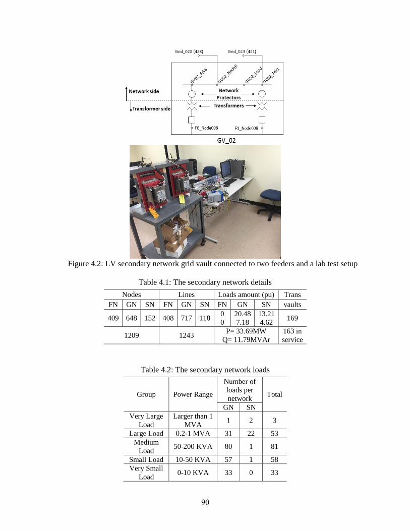
90
Figure 4.2: LV secondary network grid vault connected to two feeders and a lab test setup
Table 4.1: The secondary network details
Nodes Lines Loads amount (pu) Trans
FN GN SN FN GN SN FN GN SN vaults
409 648 152 408 717 118 0
0
20.48
7.18
13.21
4.62 169
1209 1243 P= 33.69MW
Q= 11.79MVAr
163 in
service
Table 4.2: The secondary network loads
Group Power Range
Number of
loads per
network Total
GN SN
Very Large
Load
Larger than 1
MVA 1 2 3
Large Load 0.2-1 MVA 31 22 53
Medium
Load 50-200 KVA 80 1 81
Small Load 10-50 KVA 57 1 58
Very Small
Load 0-10 KVA 33 0 33
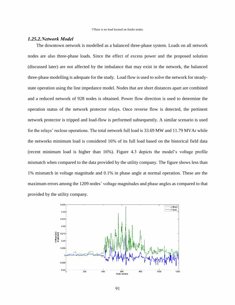
91
†There is no load located on feeder nodes.
1.25.2. Network Model
The downtown network is modelled as a balanced three-phase system. Loads on all network
nodes are also three-phase loads. Since the effect of excess power and the proposed solution
(discussed later) are not affected by the imbalance that may exist in the network, the balanced
three-phase modelling is adequate for the study. Load flow is used to solve the network for steady-
state operation using the line impedance model. Nodes that are short distances apart are combined
and a reduced network of 928 nodes is obtained. Power flow direction is used to determine the
operation status of the network protector relays. Once reverse flow is detected, the pertinent
network protector is tripped and load-flow is performed subsequently. A similar scenario is used
for the relays’ reclose operations. The total network full load is 33.69 MW and 11.79 MVAr while
the networks minimum load is considered 16% of its full load based on the historical field data
(recent minimum load is higher than 16%). Figure 4.3 depicts the model’s voltage profile
mismatch when compared to the data provided by the utility company. The figure shows less than
1% mismatch in voltage magnitude and 0.1% in phase angle at normal operation. These are the
maximum errors among the 1209 nodes’ voltage magnitudes and phase angles as compared to that
provided by the utility company.
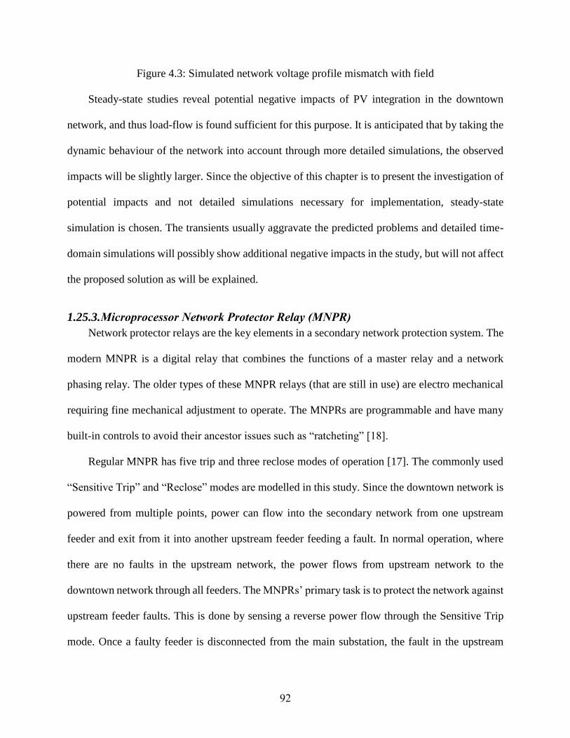
92
Figure 4.3: Simulated network voltage profile mismatch with field
Steady-state studies reveal potential negative impacts of PV integration in the downtown
network, and thus load-flow is found sufficient for this purpose. It is anticipated that by taking the
dynamic behaviour of the network into account through more detailed simulations, the observed
impacts will be slightly larger. Since the objective of this chapter is to present the investigation of
potential impacts and not detailed simulations necessary for implementation, steady-state
simulation is chosen. The transients usually aggravate the predicted problems and detailed time-
domain simulations will possibly show additional negative impacts in the study, but will not affect
the proposed solution as will be explained.
1.25.3. Microprocessor Network Protector Relay (MNPR)
Network protector relays are the key elements in a secondary network protection system. The
modern MNPR is a digital relay that combines the functions of a master relay and a network
phasing relay. The older types of these MNPR relays (that are still in use) are electro mechanical
requiring fine mechanical adjustment to operate. The MNPRs are programmable and have many
built-in controls to avoid their ancestor issues such as “ratcheting” [18].
Regular MNPR has five trip and three reclose modes of operation [17]. The commonly used
“Sensitive Trip” and “Reclose” modes are modelled in this study. Since the downtown network is
powered from multiple points, power can flow into the secondary network from one upstream
feeder and exit from it into another upstream feeder feeding a fault. In normal operation, where
there are no faults in the upstream network, the power flows from upstream network to the
downtown network through all feeders. The MNPRs’ primary task is to protect the network against
upstream feeder faults. This is done by sensing a reverse power flow through the Sensitive Trip
mode. Once a faulty feeder is disconnected from the main substation, the fault in the upstream

93
network is fed by the other feeders through the downtown network. Network protectors sense the
reverse power flow from the downtown network to the upstream feeder and disconnect the circuit.
The MNPR takes six cycles to trip and an adjustable number of cycles are required to occur for a
reclose operation. A reclose time of six cycles is considered in this study. The Sensitive Trip is set
to 0.15% of the rated transformer current [24]. The transformer protection will also trip overloaded
transformers when the loading exceeds 100% of the transformer rating. It is important to note that
the transformer rating is usually higher than the transformer nominal load. Line overload is also
considered in here by adopting 105% of the line nominal current as the overload limit. It should
be noted that the underground downtown distribution lines have lower overload tolerance than
their overhead counterparts due to the insulation material of the cables.
The reclose characteristic of the network protector relay is shown in Figure 4.4 In the figure,
reclosing voltage DV , which is the voltage difference between the two sides of the network
protector, is observed. That is, VD = VT – VN where VT is the transformer side voltage and VN is
the voltage on the network side (see Figure 4.2). If the fault exists in the upstream circuit,
transformer voltage VT lags or is smaller in magnitude than network voltage VN. The reclosing
action takes place only when the voltage on the transformer side of the open network protector is
slightly higher in magnitude and is in-phase with or leading the voltage on the network side of the
network protector. The default setting for the reclose voltage is 1.4V (this usually ranges 0.1 to
10.0V).
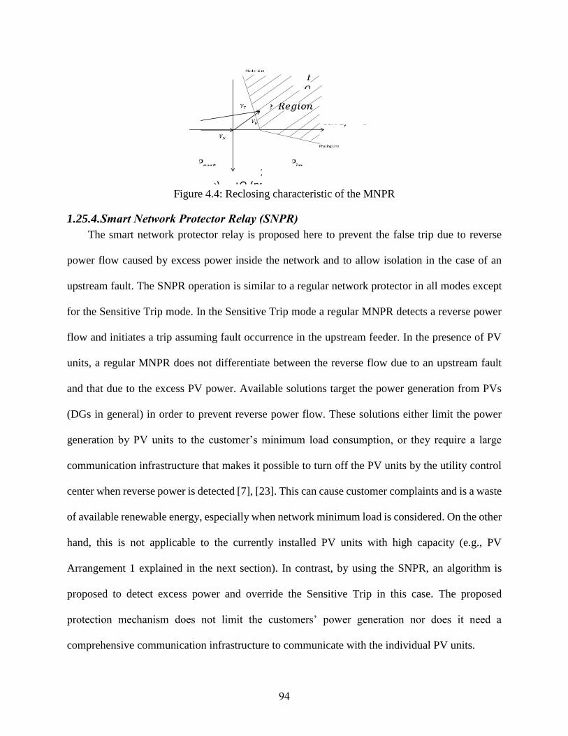
94
Figure 4.4: Reclosing characteristic of the MNPR
1.25.4. Smart Network Protector Relay (SNPR)
The smart network protector relay is proposed here to prevent the false trip due to reverse
power flow caused by excess power inside the network and to allow isolation in the case of an
upstream fault. The SNPR operation is similar to a regular network protector in all modes except
for the Sensitive Trip mode. In the Sensitive Trip mode a regular MNPR detects a reverse power
flow and initiates a trip assuming fault occurrence in the upstream feeder. In the presence of PV
units, a regular MNPR does not differentiate between the reverse flow due to an upstream fault
and that due to the excess PV power. Available solutions target the power generation from PVs
(DGs in general) in order to prevent reverse power flow. These solutions either limit the power
generation by PV units to the customer’s minimum load consumption, or they require a large
communication infrastructure that makes it possible to turn off the PV units by the utility control
center when reverse power is detected [7], [23]. This can cause customer complaints and is a waste
of available renewable energy, especially when network minimum load is considered. On the other
hand, this is not applicable to the currently installed PV units with high capacity (e.g., PV
Arrangement 1 explained in the next section). In contrast, by using the SNPR, an algorithm is
proposed to detect excess power and override the Sensitive Trip in this case. The proposed
protection mechanism does not limit the customers’ power generation nor does it need a
comprehensive communication infrastructure to communicate with the individual PV units.
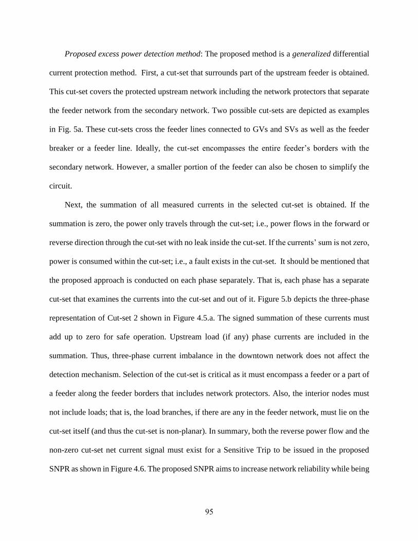
95
Proposed excess power detection method: The proposed method is a generalized differential
current protection method. First, a cut-set that surrounds part of the upstream feeder is obtained.
This cut-set covers the protected upstream network including the network protectors that separate
the feeder network from the secondary network. Two possible cut-sets are depicted as examples
in Fig. 5a. These cut-sets cross the feeder lines connected to GVs and SVs as well as the feeder
breaker or a feeder line. Ideally, the cut-set encompasses the entire feeder’s borders with the
secondary network. However, a smaller portion of the feeder can also be chosen to simplify the
circuit.
Next, the summation of all measured currents in the selected cut-set is obtained. If the
summation is zero, the power only travels through the cut-set; i.e., power flows in the forward or
reverse direction through the cut-set with no leak inside the cut-set. If the currents’ sum is not zero,
power is consumed within the cut-set; i.e., a fault exists in the cut-set. It should be mentioned that
the proposed approach is conducted on each phase separately. That is, each phase has a separate
cut-set that examines the currents into the cut-set and out of it. Figure 5.b depicts the three-phase
representation of Cut-set 2 shown in Figure 4.5.a. The signed summation of these currents must
add up to zero for safe operation. Upstream load (if any) phase currents are included in the
summation. Thus, three-phase current imbalance in the downtown network does not affect the
detection mechanism. Selection of the cut-set is critical as it must encompass a feeder or a part of
a feeder along the feeder borders that includes network protectors. Also, the interior nodes must
not include loads; that is, the load branches, if there are any in the feeder network, must lie on the
cut-set itself (and thus the cut-set is non-planar). In summary, both the reverse power flow and the
non-zero cut-set net current signal must exist for a Sensitive Trip to be issued in the proposed
SNPR as shown in Figure 4.6. The proposed SNPR aims to increase network reliability while being
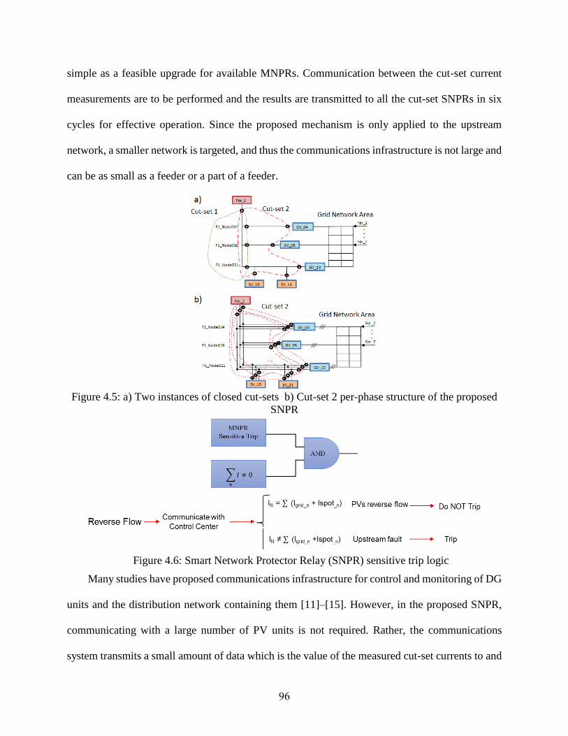
96
simple as a feasible upgrade for available MNPRs. Communication between the cut-set current
measurements are to be performed and the results are transmitted to all the cut-set SNPRs in six
cycles for effective operation. Since the proposed mechanism is only applied to the upstream
network, a smaller network is targeted, and thus the communications infrastructure is not large and
can be as small as a feeder or a part of a feeder.
Figure 4.5: a) Two instances of closed cut-sets b) Cut-set 2 per-phase structure of the proposed
SNPR
Figure 4.6: Smart Network Protector Relay (SNPR) sensitive trip logic
Many studies have proposed communications infrastructure for control and monitoring of DG
units and the distribution network containing them [11]–[15]. However, in the proposed SNPR,
communicating with a large number of PV units is not required. Rather, the communications
system transmits a small amount of data which is the value of the measured cut-set currents to and

97
from the cut-set control center, that can be one of the SNPRs. Alternatively, the current
transformers can be connected in parallel such that the current summation can be physically
obtained.
It should also be mentioned that changing the setting of the existing network protectors to
allow higher reverse power flow is challenging since high-impedance and single-phase faults,
which are low power faults in nature, may be missed and cause damage to the critical downtown
underground network. In addition, hourly and intermittent changes of solar power make the relay
setting a difficult task.
1.26. MNPR Operation
In this section, detailed studies of MNPR operation are discussed. The solar power generated
by the PV panels inside the downtown network cause changes in the feeder and line currents that
can lead to network protector false trips and/or line and transformer overloads. In the following
discussion different cases of solar and load powers are considered; then, voltage profile and
stability as well as line and transformer overloads are studied.
One of the major consequences of the network protector trips is the change in the feeders’
injected reactive and active power patterns that may lead to reactive power shortage, in the
presence of unity-power factor solar power, followed by voltage instability. As the number of
disconnected network protectors increases, network connectivity to the upstream feeder network
decreases leading to a less stable downtown network. The effect of the downtown network
connectivity on the voltage stability is studied through the lowest eigenvalue of the network
Jacobian matrix. Here, all PV units are considered as constant power generations, and thus bus
voltages are not controlled. As the minimum eigenvalue approaches zero, the Jacobian matrix
approaches singularity and more reactive power support is required to maintain the voltage.

98
1.26.1. PV Arrangements
PV power allocation varies by costumers’ locations and interest. It is reasonable to assume
that with higher PV penetration, the chances of reverse power flow is increased. The PV power
penetration can be either high-generation sites, such as large buildings or large utility-owned solar
generators, or distributed PV power generation. In the latter form, one can reasonably assume that
the amount of power generation at each node is proportional to the nominal load at that node.
Consequently, three PV arrangements are considered in this study and are referred to as
Arrangements 1, 2, and 3.
Arrangement 1 (distributed): This arrangement is comprised of distributed PV units across all
the downtown network loads. In this arrangement PV units are at 228 loaded nodes. Power of the
PV unit at each node in Arrangement 1 is varied from 15% to 150% of the full load of the node.
That is, all the PV generators experience 5%, 15%, 30%, 45%,…, and 150% of their corresponding
node’s full load, simultaneously.
Arrangement 2 (lump): This arrangement consists of 56 large PV units installed on 56 Large
and Very Large Loads (see Table II) in grid and spot networks. Total power of PV in Arrangement
2 is varied from 5% to 150% of the full load of the entire downtown network similar to the previous
case. For instance, at 150% penetration, PV Arrangement 2 has a total capacity of 1.5 times the
total downtown network full load (33.6 MW); that is, 50.4 MW is distributed among 56 PV units
proportional to their corresponding node’s load size.
Arrangement 3 (residential): This arrangement contains PV generation on the loads less than
200KW in the grid network, which are 172 loads in this study with a total of 10.12 MW power
consumption. In this arrangement, each installed PV unit generates power varying from 5% to
150% of its corresponding node’s full load similar to Arrangement 1.

99
1.26.2. MNPR Trip Statistics
The network protector’s primary task is to protect the upstream network and transformers.
The transformers connect the upstream feeders to the secondary network and are protected against
reverse power flow and overload. As the PV penetration level rises, the chances of transformer
disconnects due to reverse flow increase. Also, transformer overload can occur if a large share of
disconnected transformers is burdened on the connected ones. If all connections to a load are
disconnected, the load and its PV generator are removed from the analysis. This is usually the case
when a spot network sends power to all of its connected upstream feeders, and thus all its network
protectors trip.
The MNPRs are first simulated under hourly load and solar power for different seasons of the
year. The solar power measured by the authors, as well as the load profiles provided by the utility
company, for the full year of 2015 are utilized here. Figures 4.7.a and 4.7.c illustrate load patterns
of days with typical and minimum load profile in the summer and winter. Figure 4.7.b and 4.7.d
present normalized PV power of days with typical and maximum solar power generation in the
summer and winter. The numbers of MNPR trips are presented in Figure 4.8 using typical load
profile and typical PV power for different scenarios of PV Arrangements 1 and 2 in each season.
The PV% in the figure represents the maximum power capacity of individual PV units (that occurs
at summer noon time) with respect to their pertinent customer full load. In order to consider the
worst case, Figure 4.9 presents similar scenarios using minimum load and maximum PV power
for similar arrangements for each season. It is shown in the figures that in the cases where the solar
power is greater than that of the load (mostly around noon time) excessive MNPR trips occur,
leading to voltage instability in some cases.
Seasons From To
Spring March 16th May 15th
Summer May 16th September 7th
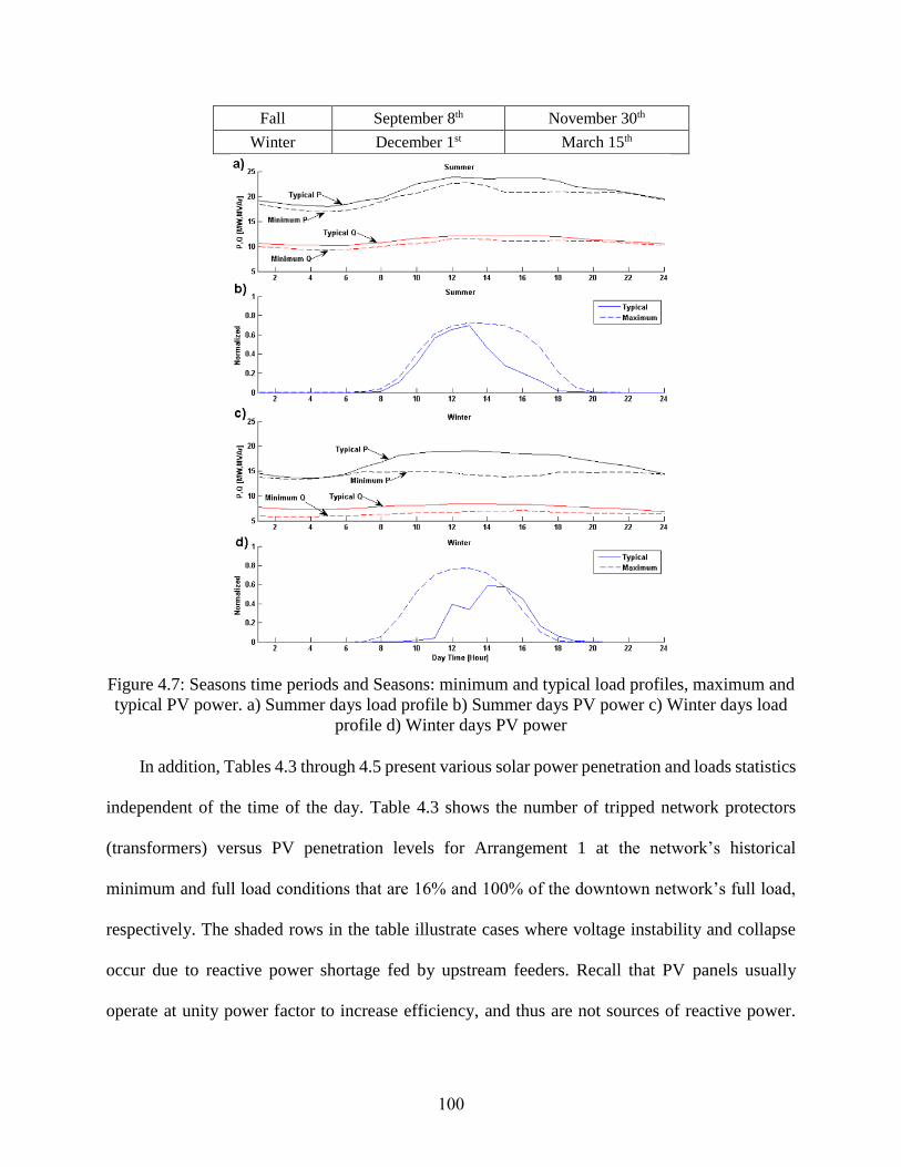
100
Fall September 8th November 30th
Winter December 1st March 15th
Figure 4.7: Seasons time periods and Seasons: minimum and typical load profiles, maximum and
typical PV power. a) Summer days load profile b) Summer days PV power c) Winter days load
profile d) Winter days PV power
In addition, Tables 4.3 through 4.5 present various solar power penetration and loads statistics
independent of the time of the day. Table 4.3 shows the number of tripped network protectors
(transformers) versus PV penetration levels for Arrangement 1 at the network’s historical
minimum and full load conditions that are 16% and 100% of the downtown network’s full load,
respectively. The shaded rows in the table illustrate cases where voltage instability and collapse
occur due to reactive power shortage fed by upstream feeders. Recall that PV panels usually
operate at unity power factor to increase efficiency, and thus are not sources of reactive power.
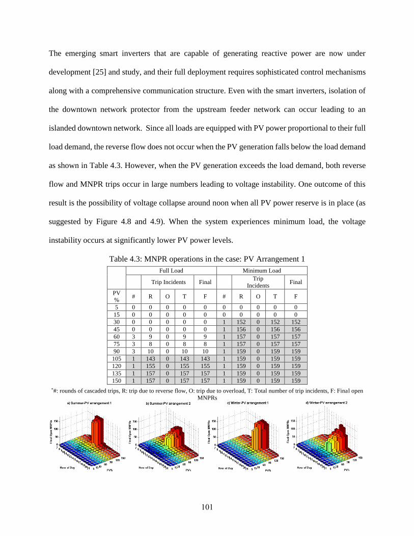
101
The emerging smart inverters that are capable of generating reactive power are now under
development [25] and study, and their full deployment requires sophisticated control mechanisms
along with a comprehensive communication structure. Even with the smart inverters, isolation of
the downtown network protector from the upstream feeder network can occur leading to an
islanded downtown network. Since all loads are equipped with PV power proportional to their full
load demand, the reverse flow does not occur when the PV generation falls below the load demand
as shown in Table 4.3. However, when the PV generation exceeds the load demand, both reverse
flow and MNPR trips occur in large numbers leading to voltage instability. One outcome of this
result is the possibility of voltage collapse around noon when all PV power reserve is in place (as
suggested by Figure 4.8 and 4.9). When the system experiences minimum load, the voltage
instability occurs at significantly lower PV power levels.
Table 4.3: MNPR operations in the case: PV Arrangement 1
Full Load Minimum Load
Trip Incidents Final Trip
Incidents Final
PV
% # R O T F # R O T F
5 0 0 0 0 0 0 0 0 0 0
15 0 0 0 0 0 0 0 0 0 0
30 0 0 0 0 0 1 152 0 152 152
45 0 0 0 0 0 1 156 0 156 156
60 3 9 0 9 9 1 157 0 157 157
75 3 8 0 8 8 1 157 0 157 157
90 3 10 0 10 10 1 159 0 159 159
105 1 143 0 143 143 1 159 0 159 159
120 1 155 0 155 155 1 159 0 159 159
135 1 157 0 157 157 1 159 0 159 159
150 1 157 0 157 157 1 159 0 159 159
*#: rounds of cascaded trips, R: trip due to reverse flow, O: trip due to overload, T: Total number of trip incidents, F: Final open
MNPRs
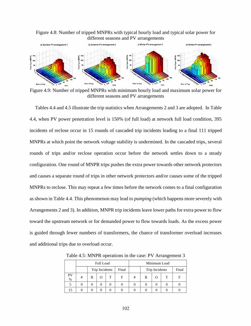
102
Figure 4.8: Number of tripped MNPRs with typical hourly load and typical solar power for
different seasons and PV arrangements
Figure 4.9: Number of tripped MNPRs with minimum hourly load and maximum solar power for
different seasons and PV arrangements
Tables 4.4 and 4.5 illustrate the trip statistics when Arrangements 2 and 3 are adopted. In Table
4.4, when PV power penetration level is 150% (of full load) at network full load condition, 395
incidents of reclose occur in 15 rounds of cascaded trip incidents leading to a final 111 tripped
MNPRs at which point the network voltage stability is undermined. In the cascaded trips, several
rounds of trips and/or reclose operation occur before the network settles down to a steady
configuration. One round of MNPR trips pushes the extra power towards other network protectors
and causes a separate round of trips in other network protectors and/or causes some of the tripped
MNPRs to reclose. This may repeat a few times before the network comes to a final configuration
as shown in Table 4.4. This phenomenon may lead to pumping (which happens more severely with
Arrangements 2 and 3). In addition, MNPR trip incidents leave lower paths for extra power to flow
toward the upstream network or for demanded power to flow towards loads. As the excess power
is guided through fewer numbers of transformers, the chance of transformer overload increases
and additional trips due to overload occur.
Table 4.5: MNPR operations in the case: PV Arrangement 3
Full Load Minimum Load
Trip Incidents Final Trip Incidents Final
PV
% # R O T F # R O T F
5 0 0 0 0 0 0 0 0 0 0
15 0 0 0 0 0 0 0 0 0 0
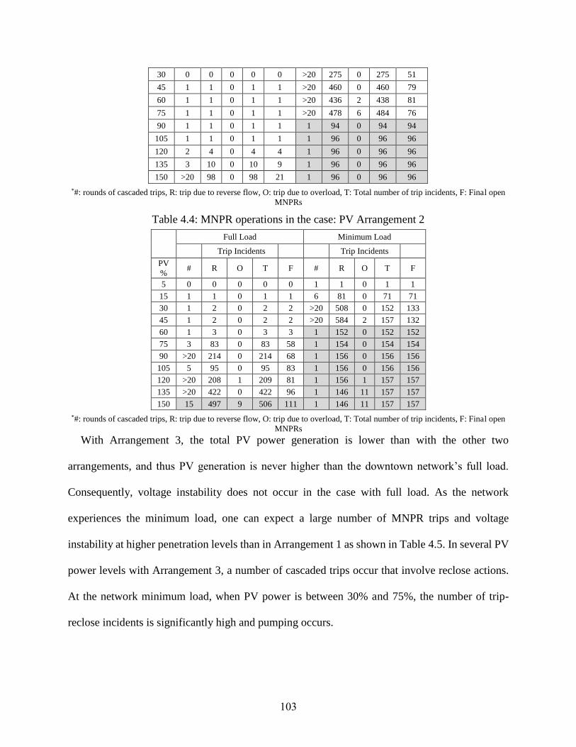
103
30 0 0 0 0 0 >20 275 0 275 51
45 1 1 0 1 1 >20 460 0 460 79
60 1 1 0 1 1 >20 436 2 438 81
75 1 1 0 1 1 >20 478 6 484 76
90 1 1 0 1 1 1 94 0 94 94
105 1 1 0 1 1 1 96 0 96 96
120 2 4 0 4 4 1 96 0 96 96
135 3 10 0 10 9 1 96 0 96 96
150 >20 98 0 98 21 1 96 0 96 96
*#: rounds of cascaded trips, R: trip due to reverse flow, O: trip due to overload, T: Total number of trip incidents, F: Final open
MNPRs
Table 4.4: MNPR operations in the case: PV Arrangement 2
Full Load Minimum Load
Trip Incidents Trip Incidents
PV
% # R O T F # R O T F
5 0 0 0 0 0 1 1 0 1 1
15 1 1 0 1 1 6 81 0 71 71
30 1 2 0 2 2 >20 508 0 152 133
45 1 2 0 2 2 >20 584 2 157 132
60 1 3 0 3 3 1 152 0 152 152
75 3 83 0 83 58 1 154 0 154 154
90 >20 214 0 214 68 1 156 0 156 156
105 5 95 0 95 83 1 156 0 156 156
120 >20 208 1 209 81 1 156 1 157 157
135 >20 422 0 422 96 1 146 11 157 157
150 15 497 9 506 111 1 146 11 157 157
*#: rounds of cascaded trips, R: trip due to reverse flow, O: trip due to overload, T: Total number of trip incidents, F: Final open
MNPRs
With Arrangement 3, the total PV power generation is lower than with the other two
arrangements, and thus PV generation is never higher than the downtown network’s full load.
Consequently, voltage instability does not occur in the case with full load. As the network
experiences the minimum load, one can expect a large number of MNPR trips and voltage
instability at higher penetration levels than in Arrangement 1 as shown in Table 4.5. In several PV
power levels with Arrangement 3, a number of cascaded trips occur that involve reclose actions.
At the network minimum load, when PV power is between 30% and 75%, the number of trip-
reclose incidents is significantly high and pumping occurs.
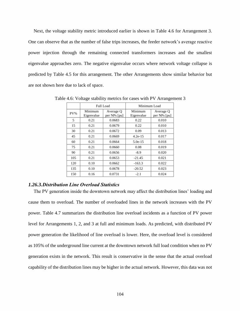
104
Next, the voltage stability metric introduced earlier is shown in Table 4.6 for Arrangement 3.
One can observe that as the number of false trips increases, the feeder network’s average reactive
power injection through the remaining connected transformers increases and the smallest
eigenvalue approaches zero. The negative eigenvalue occurs where network voltage collapse is
predicted by Table 4.5 for this arrangement. The other Arrangements show similar behavior but
are not shown here due to lack of space.
Table 4.6: Voltage stability metrics for cases with PV Arrangement 3
Full Load Minimum Load
PV% Minimum
Eigenvalue
Average Q
per NPs [pu]
Minimum
Eigenvalue
Average Q
per NPs [pu]
5 0.21 0.0683 0.22 0.010
15 0.21 0.0679 0.22 0.010
30 0.21 0.0672 0.09 0.013
45 0.21 0.0669 4.2e-15 0.017
60 0.21 0.0664 5.0e-15 0.018
75 0.21 0.0660 0.08 0.019
90 0.21 0.0656 -8.9 0.020
105 0.21 0.0653 -21.45 0.021
120 0.10 0.0662 -163.3 0.022
135 0.10 0.0678 -20.52 0.023
150 0.16 0.0731 -2.1 0.024
1.26.3. Distribution Line Overload Statistics
The PV generation inside the downtown network may affect the distribution lines’ loading and
cause them to overload. The number of overloaded lines in the network increases with the PV
power. Table 4.7 summarizes the distribution line overload incidents as a function of PV power
level for Arrangements 1, 2, and 3 at full and minimum loads. As predicted, with distributed PV
power generation the likelihood of line overload is lower. Here, the overload level is considered
as 105% of the underground line current at the downtown network full load condition when no PV
generation exists in the network. This result is conservative in the sense that the actual overload
capability of the distribution lines may be higher in the actual network. However, this data was not

105
available. Also, no line disconnect is assumed due to overload since the loadability of individual
lines were not known.
Table 4.7: Overloaded network lines in different cases
PV Arrangement 1 PV Arrangement 2 PV Arrangement 3
PV% Full
load
Min
load
Full
load
Min
load
Full
load
Min
load
5 0 0 8 0 16 0
15 0 0 44 35 38 5
30 0 n/a 72 96 48 34
45 0 n/a 89 188 60 118
60 0 n/a 99 n/a 70 121
75 0 n/a 132 n/a 75 185
90 0 n/a 139 n/a 81 n/a
105 n/a n/a 221 n/a 90 n/a
120 n/a n/a 239 n/a 109 n/a
135 n/a n/a 301 n/a 115 n/a
150 n/a n/a n/a n/a 151 n/a
1.26.4. MNPR Reclose operation
The default reclose voltage setting of the relay simulated in this study is 1.4V (VD=1.4V) [24].
The relay reclose voltage setting establishes the minimum difference voltage required to issue a
reclose command when the feeder voltage and network voltage are in phase. With the default
reclose setting, a number of network protectors that are tripped due to reverse power flow will
reclose after the reclose cycle has passed. A solar power penetration scenario is arranged to show
the pumping effect. At the MNPR in Grid Vault 29 fed by Feeder 4, the voltage difference is VD
= 1.87V > 1.4V; and at the MNPR in Grid Vault 44 fed by Feeder 7, VD = 1.62V > 1.4V after the
trip due to reverse power flow. Thus, the two network protectors in the vaults are ready to reclose.
However, after MNPRs reclosed, both transformers see reverse power again and subsequently trip.
This process will continue leading to excessive relay operations which is known as pumping [20].
Allowing the network protector to close with a small difference voltage magnitude can lead to
pumping in certain arrangements and penetration levels as observed. However, it can be seen
that when the threshold is increased to 2V, pumping does not occur when the MNPR is used. As
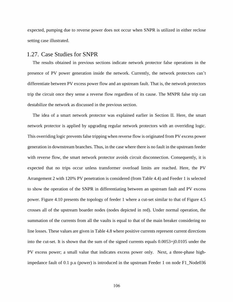
106
expected, pumping due to reverse power does not occur when SNPR is utilized in either reclose
setting case illustrated.
1.27. Case Studies for SNPR
The results obtained in previous sections indicate network protector false operations in the
presence of PV power generation inside the network. Currently, the network protectors can’t
differentiate between PV excess power flow and an upstream fault. That is, the network protectors
trip the circuit once they sense a reverse flow regardless of its cause. The MNPR false trip can
destabilize the network as discussed in the previous section.
The idea of a smart network protector was explained earlier in Section II. Here, the smart
network protector is applied by upgrading regular network protectors with an overriding logic.
This overriding logic prevents false tripping when reverse flow is originated from PV excess power
generation in downstream branches. Thus, in the case where there is no fault in the upstream feeder
with reverse flow, the smart network protector avoids circuit disconnection. Consequently, it is
expected that no trips occur unless transformer overload limits are reached. Here, the PV
Arrangement 2 with 120% PV penetration is considered (from Table 4.4) and Feeder 1 is selected
to show the operation of the SNPR in differentiating between an upstream fault and PV excess
power. Figure 4.10 presents the topology of feeder 1 where a cut-set similar to that of Figure 4.5
crosses all of the upstream boarder nodes (nodes depicted in red). Under normal operation, the
summation of the currents from all the vaults is equal to that of the main breaker considering no
line losses. These values are given in Table 4.8 where positive currents represent current directions
into the cut-set. It is shown that the sum of the signed currents equals 0.0053+j0.0105 under the
PV excess power; a small value that indicates excess power only. Next, a three-phase high-
impedance fault of 0.1 p.u (power) is introduced in the upstream Feeder 1 on node F1_Node036
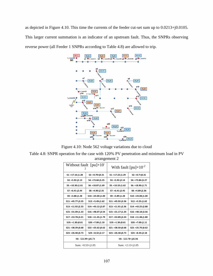
107
as depicted in Figure 4.10. This time the currents of the feeder cut-set sum up to 0.0213+j0.0105.
This larger current summation is an indicator of an upstream fault. Thus, the SNPRs observing
reverse power (all Feeder 1 SNPRs according to Table 4.8) are allowed to trip.
Figure 4.10: Node 562 voltage variations due to cloud
Table 4.8: SNPR operation for the case with 120% PV penetration and minimum load in PV
arrangement 2 Without fault [pu]×10-
2 With fault [pu]×10-2
S1: +17.16-j1.28 S2: +0.70+j0.31 S1: +17.22-j1.29 S2: +0.7+j0.31
S3: +5.92-j2.13 S4: +73.60-j5.25 S3: +5.92-j2.14 S4: +73.84-j5.27
S5: +10.30-j1.61 S6: +18.87-j1.69 S5: +10.33-j1.62 S6: +18.90-j1.71
S7: +6.41-j2.44 S8: +4.90-j2.35 S7: +6.41-j2.45 S8: +4.89-j2.36
S9: +3.88-j1.28 S10: +24.00-j1.00 S9: +3.89-j1.28 S10: +24.08-j1.00
S11: +45.77-j3.35 S12: +5.49-j1.62 S11: +45.92-j3.36 S12: +5.55-j1.62
S13: +11.92-j2.33 S14: +43.12-j2.87 S13: +11.91-j2.36 S14: +43.25-j2.88
S15: +31.09-j1.33 S16: +48.07-j3.54 S15: +31.17-j1.34 S16: +48.18-j3.56
S17: +53.78-j3.21 S18: +11.45-j1.79 S17: +53.89-j3.24 S18: +11.48-j1.80
S19: +1.30-j0.61 S20: +7.00-j1.10 S19: +1.30-j0.61 S20: +7.00-j1.11
S21: +38.39-j0.68 S22: +25.62-j0.62 S21: +38.50-j0.68 S22: +25.70-j0.62
S23: +26.48-j0.73 S24: +8.32-j2.17 S23: +26.58-j0.73 S24: +8.34-j2.18
S0: -522.99+j45.73 S0: -522.78+j45.94
Sum: +0.53+j1.05 Sum: +2.13+j1.05

108
1.28. Cloud Effect
The intermittent nature of PV power causes injected power variations at downtown network
nodes. In this research scattered cloud is considered by randomly assigning power drop at PV
generation locations throughout the secondary network at high PV power levels. Satellite data for
sun irradiance has been purchased and is being recorded for two sites, one in Baton Rouge, LSU
location and the other one in New Orleans, French Quarter. Figure 4.11 presents the exact locations
for these sites. Satellite data provides knowledge of solar radiation and effects of wind, cloud or
any other natural element on the received solar energy on the earth. The satellite data will be
recorded for a complete year starting Dec 1, 2014. However, the satellite data is recorder every
minute. Also, the accuracy of the received solar power on earth via the satellite data in unknown.
Thus, an experimental setup is prepared and installed at LSU to record the received solar power
on the earth with higher time resolution.
Figure 4.11: The two sites in New Orleans and Baton Rouge for Solar Satellite data
acquisition
In order to generate the random power, first solar power is measured over a course of three
months in winter 2015 (where solar power variation is significant) at the Louisiana State
University. The PV power is measured through a 140-Watt solar panel connected to a resistive

109
load. The Fluke-43B data acquisition system is used along with LabVIEW software to capture the
voltage every four seconds. The solar power measurement setup is shown in Figure 4.2. Next, one
of the days in winter with most PV power variation is chosen and maximum power level fall and
duration are obtained. Then, cloud assignment is conducted by considering 𝑇𝑢𝑝 = −𝑎 × 𝑙𝑛𝑈1 and
𝑇𝑑𝑜𝑤𝑛 = −𝑏 × 𝑙𝑛𝑈2 where 𝑈1 and 𝑈2 are uniformly distributed random numbers in the range
[0,1] and a and b are average up and down times in the solar irradiation. The power drop is also
generated through uniformly distributed random number in the range of zero to 60% solar
irradiance drop. Subsequently, 228 random variable powers are generated using the random
distribution functions explained above and are applied to all load nodes in Arrangement 1 at 100%
(of full load) penetration level. At this level no reverse power is observed by MNPRs and thus no
MNPR trips occur. It is observed that at some nodes, voltage flicker in the range of “irritative”
occurs as shown in Figure 4.14 based on IEEE 519 definitions [21]. Also, some nodes experience
visible flicker [21]. With SNPR and higher PV power levels voltage flicker increases.
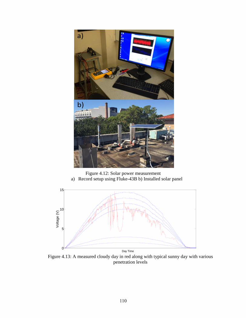
110
Figure 4.12: Solar power measurement
a) Record setup using Fluke-43B b) Installed solar panel
Figure 4.13: A measured cloudy day in red along with typical sunny day with various
penetration levels
a)
b)
0
5
10
15
Vo
lta
ge
(V
)
Day Time
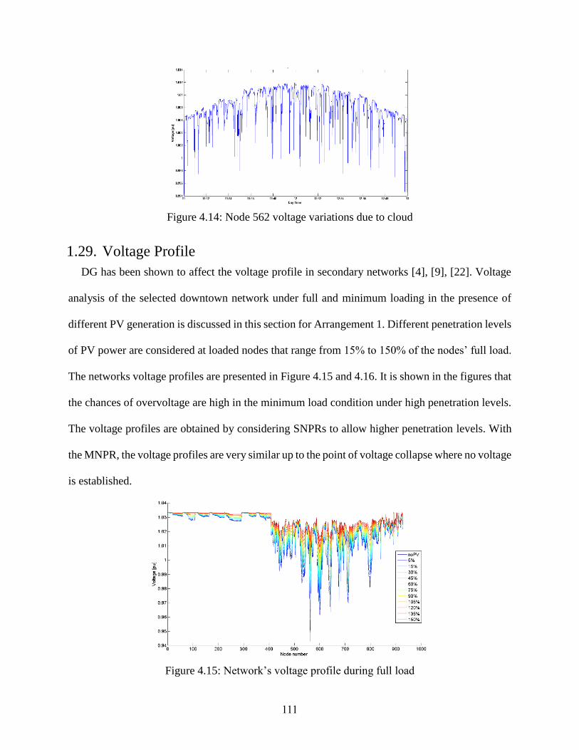
111
Figure 4.14: Node 562 voltage variations due to cloud
1.29. Voltage Profile
DG has been shown to affect the voltage profile in secondary networks [4], [9], [22]. Voltage
analysis of the selected downtown network under full and minimum loading in the presence of
different PV generation is discussed in this section for Arrangement 1. Different penetration levels
of PV power are considered at loaded nodes that range from 15% to 150% of the nodes’ full load.
The networks voltage profiles are presented in Figure 4.15 and 4.16. It is shown in the figures that
the chances of overvoltage are high in the minimum load condition under high penetration levels.
The voltage profiles are obtained by considering SNPRs to allow higher penetration levels. With
the MNPR, the voltage profiles are very similar up to the point of voltage collapse where no voltage
is established.
Figure 4.15: Network’s voltage profile during full load
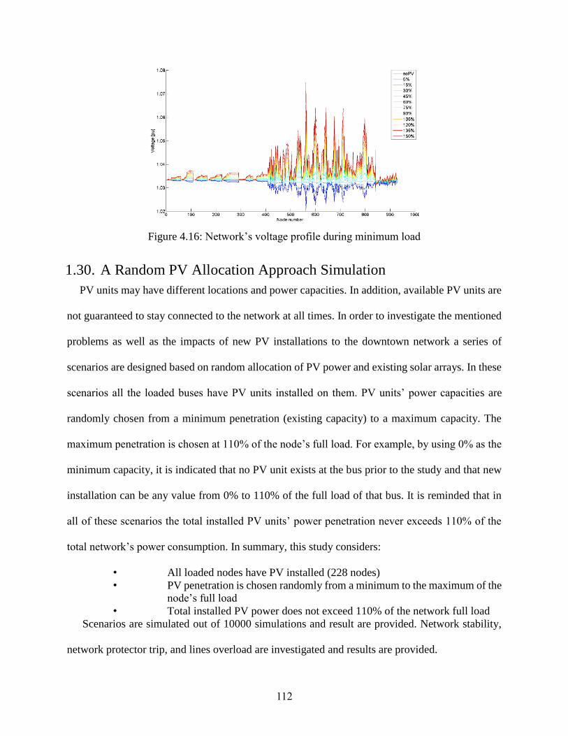
112
Figure 4.16: Network’s voltage profile during minimum load
1.30. A Random PV Allocation Approach Simulation
PV units may have different locations and power capacities. In addition, available PV units are
not guaranteed to stay connected to the network at all times. In order to investigate the mentioned
problems as well as the impacts of new PV installations to the downtown network a series of
scenarios are designed based on random allocation of PV power and existing solar arrays. In these
scenarios all the loaded buses have PV units installed on them. PV units’ power capacities are
randomly chosen from a minimum penetration (existing capacity) to a maximum capacity. The
maximum penetration is chosen at 110% of the node’s full load. For example, by using 0% as the
minimum capacity, it is indicated that no PV unit exists at the bus prior to the study and that new
installation can be any value from 0% to 110% of the full load of that bus. It is reminded that in
all of these scenarios the total installed PV units’ power penetration never exceeds 110% of the
total network’s power consumption. In summary, this study considers:
• All loaded nodes have PV installed (228 nodes)
• PV penetration is chosen randomly from a minimum to the maximum of the
node’s full load
• Total installed PV power does not exceed 110% of the network full load
Scenarios are simulated out of 10000 simulations and result are provided. Network stability,
network protector trip, and lines overload are investigated and results are provided.
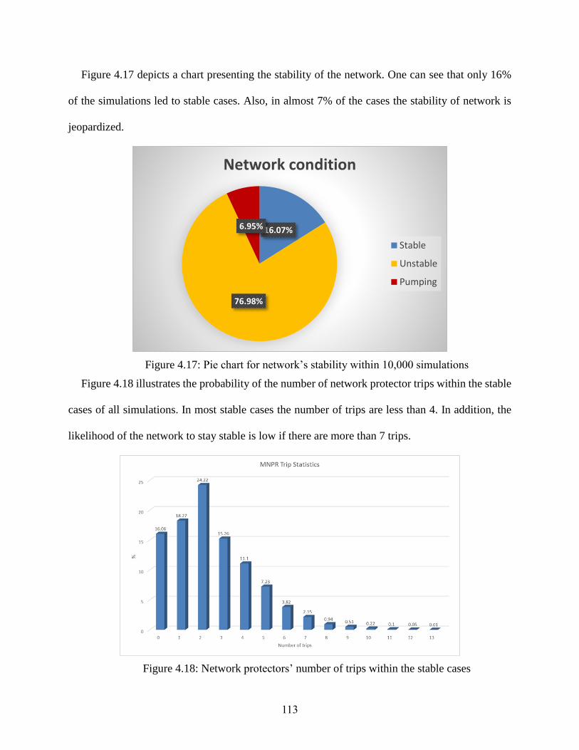
113
Figure 4.17 depicts a chart presenting the stability of the network. One can see that only 16%
of the simulations led to stable cases. Also, in almost 7% of the cases the stability of network is
jeopardized.
Figure 4.17: Pie chart for network’s stability within 10,000 simulations
Figure 4.18 illustrates the probability of the number of network protector trips within the stable
cases of all simulations. In most stable cases the number of trips are less than 4. In addition, the
likelihood of the network to stay stable is low if there are more than 7 trips.
Figure 4.18: Network protectors’ number of trips within the stable cases
16.07%
76.98%
6.95%
Network condition
Stable
Unstable
Pumping
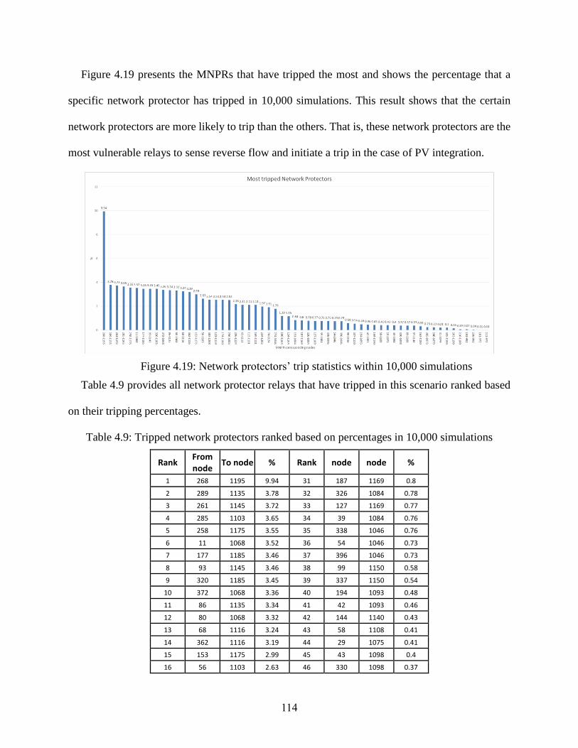
114
Figure 4.19 presents the MNPRs that have tripped the most and shows the percentage that a
specific network protector has tripped in 10,000 simulations. This result shows that the certain
network protectors are more likely to trip than the others. That is, these network protectors are the
most vulnerable relays to sense reverse flow and initiate a trip in the case of PV integration.
Figure 4.19: Network protectors’ trip statistics within 10,000 simulations
Table 4.9 provides all network protector relays that have tripped in this scenario ranked based
on their tripping percentages.
Table 4.9: Tripped network protectors ranked based on percentages in 10,000 simulations
Rank From node To node % Rank node node %
1 268 1195 9.94 31 187 1169 0.8 2 289 1135 3.78 32 326 1084 0.78 3 261 1145 3.72 33 127 1169 0.77 4 285 1103 3.65 34 39 1084 0.76 5 258 1175 3.55 35 338 1046 0.76 6 11 1068 3.52 36 54 1046 0.73 7 177 1185 3.46 37 396 1046 0.73 8 93 1145 3.46 38 99 1150 0.58 9 320 1185 3.45 39 337 1150 0.54
10 372 1068 3.36 40 194 1093 0.48 11 86 1135 3.34 41 42 1093 0.46 12 80 1068 3.32 42 144 1140 0.43 13 68 1116 3.24 43 58 1108 0.41 14 362 1116 3.19 44 29 1075 0.41 15 153 1175 2.99 45 43 1098 0.4 16 56 1103 2.63 46 330 1098 0.37
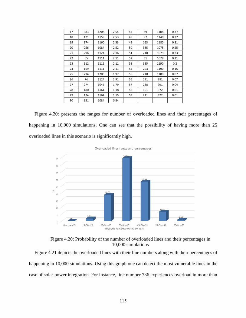
115
17 383 1208 2.54 47 89 1108 0.37 18 121 1159 2.53 48 97 1140 0.37 19 174 1160 2.53 49 163 1180 0.31 20 256 1084 2.52 50 385 1075 0.25 21 296 1124 2.16 51 240 1079 0.23 22 65 1111 2.11 52 31 1079 0.21 23 112 1111 2.11 53 335 1190 0.2 24 169 1111 2.11 54 203 1190 0.15 25 234 1203 1.97 55 210 1180 0.07 26 74 1124 1.91 56 191 991 0.07 27 274 1046 1.79 57 238 991 0.04 28 180 1164 1.18 58 161 972 0.01 29 124 1164 1.15 59 211 972 0.01 30 151 1084 0.84
Figure 4.20: presents the ranges for number of overloaded lines and their percentages of
happening in 10,000 simulations. One can see that the possibility of having more than 25
overloaded lines in this scenario is significantly high.
Figure 4.20: Probability of the number of overloaded lines and their percentages in
10,000 simulations
Figure 4.21 depicts the overloaded lines with their line numbers along with their percentages of
happening in 10,000 simulations. Using this graph one can detect the most vulnerable lines in the
case of solar power integration. For instance, line number 736 experiences overload in more than
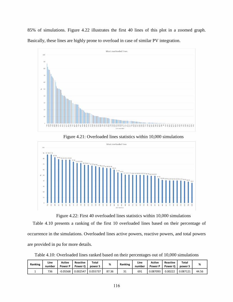
116
85% of simulations. Figure 4.22 illustrates the first 40 lines of this plot in a zoomed graph.
Basically, these lines are highly prone to overload in case of similar PV integration.
Figure 4.21: Overloaded lines statistics within 10,000 simulations
Figure 4.22: First 40 overloaded lines statistics within 10,000 simulations
Table 4.10 presents a ranking of the first 10 overloaded lines based on their percentage of
occurrence in the simulations. Overloaded lines active powers, reactive powers, and total powers
are provided in pu for more details.
Table 4.10: Overloaded lines ranked based on their percentages out of 10,000 simulations
Ranking Line
number Active
Power P
Reactive Power Q
Total power S
% Ranking Line
number Active
Power P
Reactive Power Q
Total power S
%
1 736 -0.05568 0.002547 0.055737 87.36 31 691 0.087093 0.00222 0.087121 44.56
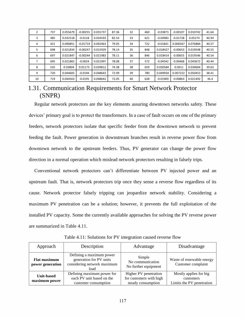
117
2 737 0.055679 -0.00255 0.055737 87.36 32 460 -0.03873 -0.00107 0.010742 41.64 3 485 0.032518 -0.0118 0.034593 82.54 33 621 -0.04983 -0.01728 0.05274 40.94 4 421 0.090851 -0.01719 0.092463 79.05 34 722 -0.01841 0.006567 0.076884 40.57 5 698 0.021834 -0.00247 0.015929 78.14 35 848 0.018427 -0.00653 0.019548 40.55 6 697 0.021847 -0.00244 0.021983 78.11 36 846 0.018414 -0.00655 0.019546 40.54 7 695 0.021865 -0.0024 0.021997 78.08 37 572 -0.04342 -0.00468 0.043672 40.44 8 535 -0.03804 0.01173 0.039812 74.38 38 659 0.030584 -0.0011 0.030604 39.63 9 720 0.044605 -0.0194 0.048643 72.09 39 780 0.049934 0.007222 0.050453 38.41
10 719 0.044563 -0.0195 0.048642 72.05 40 628 -0.01969 -0.00863 0.021492 36.4
1.31. Communication Requirements for Smart Network Protector
(SNPR)
Regular network protectors are the key elements assuring downtown networks safety. These
devices’ primary goal is to protect the transformers. In a case of fault occurs on one of the primary
feeders, network protectors isolate that specific feeder from the downtown network to prevent
feeding the fault. Power generation in downstream branches result in reverse power flow from
downtown network to the upstream feeders. Thus, PV generator can change the power flow
direction in a normal operation which mislead network protectors resulting in falsely trips.
Conventional network protectors can’t differentiate between PV injected power and an
upstream fault. That is, network protectors trip once they sense a reverse flow regardless of its
cause. Network protector falsely tripping can jeopardize network stability. Considering a
maximum PV penetration can be a solution; however, it prevents the full exploitation of the
installed PV capacity. Some the currently available approaches for solving the PV reverse power
are summarized in Table 4.11.
Table 4.11: Solutions for PV integration caused reverse flow
Approach Description Advantage Disadvantage
Flat maximum
power generation
Defining a maximum power
generation for PV units
considering network maximum
load
Simple
No communication
No further equipment
Waste of renewable energy
Customer complaint
Unit-based
maximum power
Defining maximum power for
each PV unit based on the
customer consumption
Higher PV penetration
for customers with high
steady consumption
Mostly applies for big
customers
Limits the PV penetration

118
Economical
Displaceable
units
Disconnecting PV units once
they exceed exporting power
using communication
Adaptable approach
Higher PV penetration
level
Provides monitoring
Requires network-wide
communication
infrastructure
Limits the PV penetration
Smart Network
Protector Relays
(SNPR)
SNPR differentiates between PV
reverse power and upstream
fault
Relatively simple to
implement
Adaptable approach
Exploits maximum
possible PV penetration
Provides monitoring
Requires fast but limited
upstream communication
1.31.1. Smart Network Protector Relay (SNPR)
Network protector relays sensitive mode observes current angles with respect to voltage phase
angles. This is how the current direction can be identified. The directions of power and current are
considered based on the active power direction. Figure 4.23 presents network protector’s sensitive
mode characteristics along with the active power direction. From Figure 4.23, network protector
relays should trip once the current and power fall in to the 2nd and 3rd quarters in the left hand side
of the solid line.
Figure 4.23: Network protector sensitive mode characteristics
The idea pf smart network protector is applicable by upgrading regular network protectors with
an overriding logic. This overriding logic prevents false tripping when reverse flow is originated
from the PV excessive power generation in the downtown network. This upgrading logic is
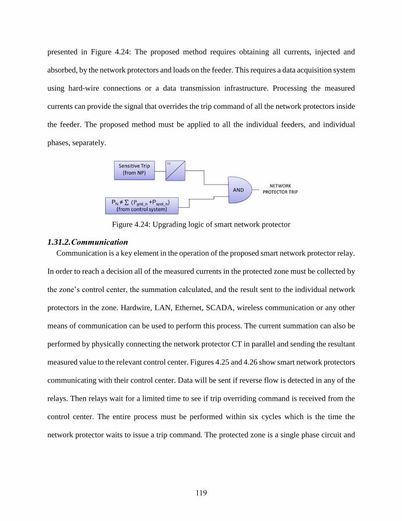
119
presented in Figure 4.24: The proposed method requires obtaining all currents, injected and
absorbed, by the network protectors and loads on the feeder. This requires a data acquisition system
using hard-wire connections or a data transmission infrastructure. Processing the measured
currents can provide the signal that overrides the trip command of all the network protectors inside
the feeder. The proposed method must be applied to all the individual feeders, and individual
phases, separately.
Figure 4.24: Upgrading logic of smart network protector
1.31.2. Communication
Communication is a key element in the operation of the proposed smart network protector relay.
In order to reach a decision all of the measured currents in the protected zone must be collected by
the zone’s control center, the summation calculated, and the result sent to the individual network
protectors in the zone. Hardwire, LAN, Ethernet, SCADA, wireless communication or any other
means of communication can be used to perform this process. The current summation can also be
performed by physically connecting the network protector CT in parallel and sending the resultant
measured value to the relevant control center. Figures 4.25 and 4.26 show smart network protectors
communicating with their control center. Data will be sent if reverse flow is detected in any of the
relays. Then relays wait for a limited time to see if trip overriding command is received from the
control center. The entire process must be performed within six cycles which is the time the
network protector waits to issue a trip command. The protected zone is a single phase circuit and
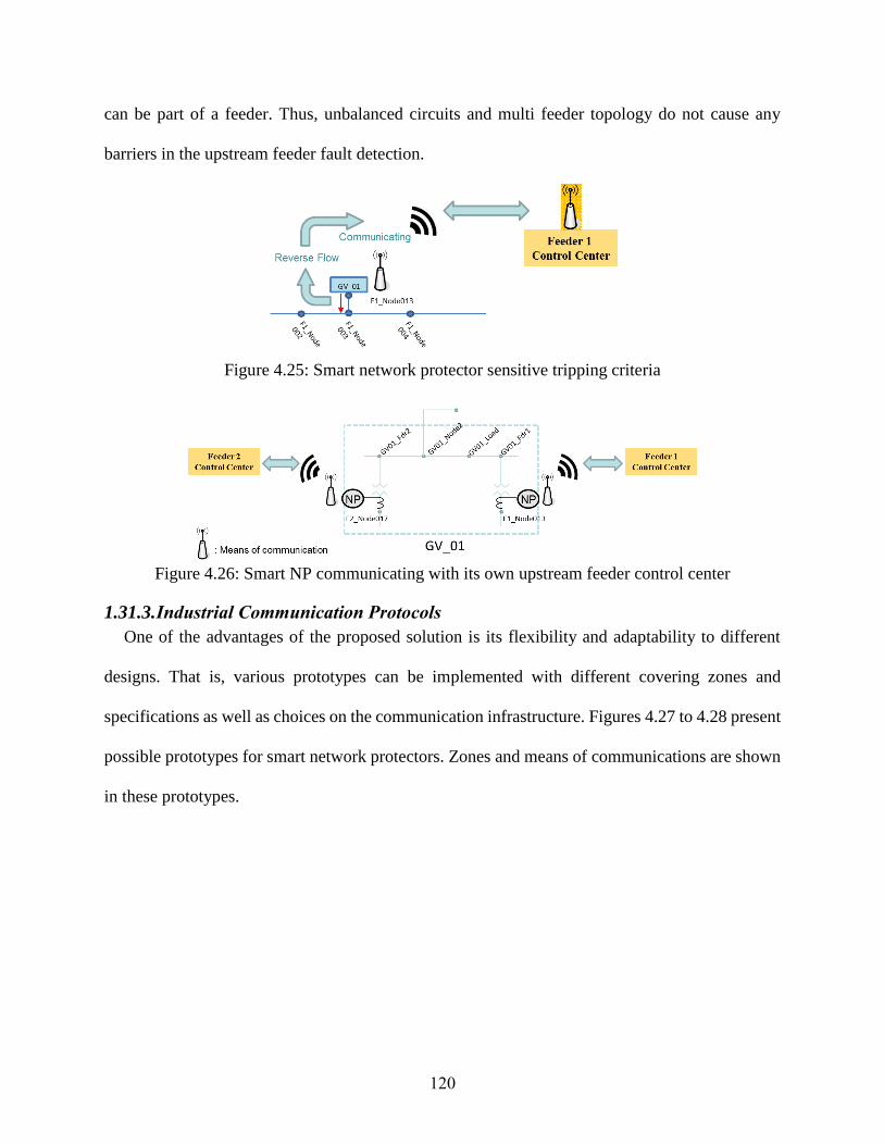
120
can be part of a feeder. Thus, unbalanced circuits and multi feeder topology do not cause any
barriers in the upstream feeder fault detection.
Figure 4.25: Smart network protector sensitive tripping criteria
Figure 4.26: Smart NP communicating with its own upstream feeder control center
1.31.3. Industrial Communication Protocols
One of the advantages of the proposed solution is its flexibility and adaptability to different
designs. That is, various prototypes can be implemented with different covering zones and
specifications as well as choices on the communication infrastructure. Figures 4.27 to 4.28 present
possible prototypes for smart network protectors. Zones and means of communications are shown
in these prototypes.
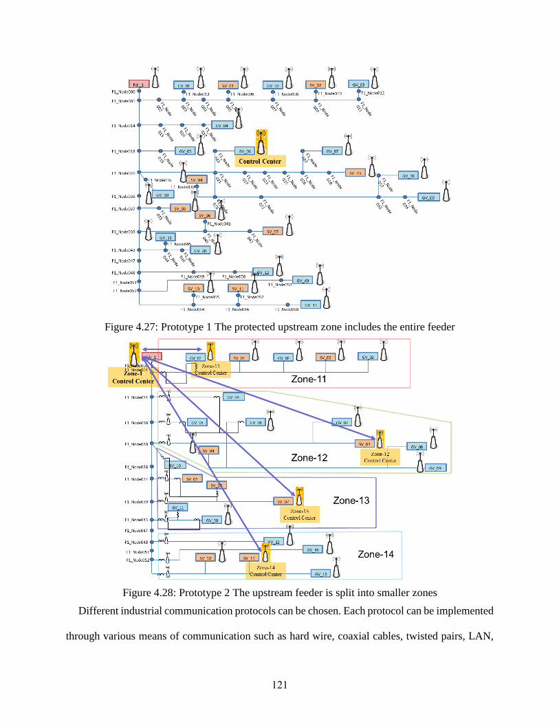
121
Figure 4.27: Prototype 1 The protected upstream zone includes the entire feeder
Figure 4.28: Prototype 2 The upstream feeder is split into smaller zones
Different industrial communication protocols can be chosen. Each protocol can be implemented
through various means of communication such as hard wire, coaxial cables, twisted pairs, LAN,

122
Ethernet, and wireless communication. For instance, for vaults locating close to one another hard
wire communication may be preferred. A list of popular and applicable communication protocols
includes Industrial Ethernet, DNP3, Modbus, CanOpen, DeviceNet, Profibus, Fieldbus, etc. Also,
some proprietary protocols can also be chosen, including SPA (ABB), VDEW (Siemens), and K-
BUS (Alstom).
Table 4.12 provides a list of most common and applicable industrial protocols. An estimation
of speed is provided for each of these protocols along with possible means of communication.
Table 4.12: Industrial communication protocols and estimated design specification
Protocol Implementation Bit rate Max Distance Max
Industrial
Ethernet
Coax, twisted pair,
fiber 10, 100 Mbps 100 m up to Km 1024
Modbus
RTU/ASCII Twisted pair
300 bps-
38.4Kbps
350 m (for RS-
485) 250
DNP3 Twisted pair, fiber,
wireless, Ethernet 300-1200 bps Long Multiple
CANopen Twisted pair 10K-1Mbps 25-1000 m 127
DeviceNet Twisted pair 125-500Kbps 500m-6Km 64
PROFIBUS Twisted pair, fiber 9.6K-12Mbps 100m 127
Fieldbus Twisted pair, fiber 31.25K-5Mbps 500-1700m 127
Ethernet is the most updated and promising capabilities as required for SNPR implementation.
Some of the advantages of Ethernet include:
- Abundant hardware availability (vast number of suppliers)
- Security and Reliability by IP addressing
- Scalability and flexibility (easy to expand)
- Easy design and programming with user interface enabled
- Can transfer power by PoE technology as well as any form of data
- Record and monitoring features.
Ethernet design is simple as long as nodes are located within 1000 meter from one another. This
will mandate zoning in any design and prototype chosen for SNPR implementation. The

123
communication delay can be reduced by choosing fast microprocessor units. Processing will not
be a preventive factor due to the simple math and algorithm involved. Current measurement and
handshaking signals of a large number of nodes can be accommodated in the Ethernet through
1500 Bytes. These data are required to be transmitted from all nodes in a selected zone through
Ethernet. Considering an Ethernet with 10 Mbps bit rate, one can calculate the communication
delay time as: (1500×8)/10,000,000 = 0.0012 sec or 1.2 msec.
One can see that by using 10Mbps, the SNPR can scan the measured data several times within
the six cycle time span. Using the same procedure, the final delay time can be calculated for
Ethernet with 50 and 100 Mbps as:
- Ethernet 50 Mbps speed: 0.48 ms
- Ethernet 100 Mbps speed: 0.24 ms
Hence, using a higher Ethernet speed results in higher speed. This can avoid possible false
decisions due to transients which are common in downtown networks.
1.32. Conclusion
Operational challenges of network protectors in downtown networks in the presence of PV
power integration are discussed in this chapter. A model is developed for the downtown network
based on line impedance models, and load flow is performed to simulate the network operation.
Distributed PV unit arrangements are utilized and the results are compared. It is demonstrated that
large network protector trips can occur in the presence of PV power leading to potential network
voltage collapse. Smart network protectors that distinguish between upstream faults and PV excess
power are proposed, and network operation is compared with and without the smart network
protectors. Finally, voltage profile and flicker are shown to be affected by the PV power installed
in the downtown network.
124
1.33. References
[1] Katiraei, F.; Aguero, J.R., "Solar PV Integration Challenges," Power and Energy
Magazine, IEEE , vol.9, no.3, pp.62,71, May-June 2011.
[2] Walling, R.A. ; Saint, R.; Dugan, R.C.; Burke, J.; Kojovic, L.A., "Summary of
Distributed Resources Impact on Power Delivery Systems," Power Delivery, IEEE
Transactions on , vol.23, no.3, pp.1636,1644, July 2008.
[3] U.S. Solar Market Insight Report, Q1 2015, executive summary. [Online] Available:
http://www.seia.org/research-resources/solar-market-insight-report-2015-q1
[4] Po-Chen Chen; Salcedo, R.; Qingcheng Zhu; de Leon, F.; Czarkowski, D.; Zhong-Ping
Jiang; Spitsa, V.; Zabar, Z.; Uosef, R.E., "Analysis of Voltage Profile Problems Due to
the Penetration of Distributed Generation in Low-Voltage Secondary Distribution
Networks," Power Delivery, IEEE Transactions on , vol.27, no.4, pp.2020,2028, Oct.
2012.
[5] Ochoa, L.F.; Harrison, G.P., "Minimizing Energy Losses: Optimal Accommodation
and Smart Operation of Renewable Distributed Generation," Power Systems, IEEE
Transactions on , vol.26, no.1, pp.198,205, Feb. 2011.
[6] Brown, T., "Transmission network loading in Europe with high shares of
renewables," Renewable Power Generation, IET , vol.9, no.1, pp.57,65, 1 2015.
[7] Tonkoski, R.; Lopes, L.A.C.; El-Fouly, T.H.M., "Coordinated Active Power
Curtailment of Grid Connected PV Inverters for Overvoltage Prevention," Sustainable
Energy, IEEE Transactions on , vol.2, no.2, pp.139,147, April 2011.
[8] Hooshyar, H.; Baran, M.E., "Fault Analysis on Distribution Feeders With High
Penetration of PV Systems," Power Systems, IEEE Transactions on , vol.28, no.3,
pp.2890,2896, Aug. 2013.
[9] Baran, M.E.; Hooshyar, H.; Zhan Shen; Huang, A., "Accommodating High PV
Penetration on Distribution Feeders," Smart Grid, IEEE Transactions on , vol.3, no.2,
pp.1039,1046, June 2012.
[10] Cheung, H.; Hamlyn, A.; Lin Wang; Cungang Yang; Cheung, R., "Investigations
of impacts of distributed generations on feeder protections," Power & Energy Society
General Meeting, 2009. PES '09. IEEE , vol., no., pp.1,7, 26-30 July 2009.
[11] Yazdanpanahi, H.; Yun Wei Li; Wilsun Xu, "A New Control Strategy to Mitigate
the Impact of Inverter-Based DGs on Protection System," Smart Grid, IEEE
Transactions on , vol.3, no.3, pp.1427,1436, Sept. 2012.
[12] Alam, M.J.E.; Muttaqi, K.M.; Sutanto, D., "Mitigation of Rooftop Solar PV
Impacts and Evening Peak Support by Managing Available Capacity of Distributed
Energy Storage Systems," Power Systems, IEEE Transactions on , vol.28, no.4,
pp.3874,3884, Nov. 2013.
[13] Alam, M.J.E.; Muttaqi, K.M.; Sutanto, D., "An Approach for Online Assessment
of Rooftop Solar PV Impacts on Low-Voltage Distribution Networks," Sustainable
Energy, IEEE Transactions on , vol.5, no.2, pp.663,672, April 2014.

125
[14] Zamani, M.A.; Yazdani, A.; Sidhu, T.S., "A Communication-Assisted Protection
Strategy for Inverter-Based Medium-Voltage Microgrids," Smart Grid, IEEE
Transactions on , vol.3, no.4, pp.2088,2099, Dec. 2012.
[15] Schweitzer, E.O.; Finney, D.; Mynam, M.V., "Applying radio communication in
distribution generation teleprotection schemes," Protective Relay Engineers, 2012 65th
Annual Conference for , vol., no., pp.310,320, 2-5 April 2012.
[16] Li Yu; Czarkowski, D.; De Leon, F.; Bury, W., "A time sequence load-flow method
for steady-state analysis in heavily meshed distribution network with
DG," Compatibility and Power Electronics (CPE), 2013 8th International Conference
on , vol., no., pp.25,30, 5-7 June 2013.
[17] Wei-Jen Lee; Cultrera, J.; Maffetone, T., "Application and testing of a
microcomputer-based network protector," Industry Applications, IEEE Transactions
on , vol.36, no.2, pp.691,696, Mar/Apr 2000.
[18] IEEE Application Guide for IEEE Std 1547(TM), IEEE Standard for
Interconnecting Distributed Resources with Electric Power Systems," IEEE Std
1547.2-2008 , vol., no., pp.1,217, April 15 2009.
[19] IEEE Recommended Practice for Protection and Coordination of Industrial and
Commercial Power Systems (IEEE Buff Book)," IEEE Std 242-2001 (Revision of IEEE
Std 242-1986) [IEEE Buff Book] , vol., no., pp.1,710, Dec. 17 2001.
[20] IEEE Standard Requirements for Secondary Network Protectors," IEEE Std
C57.12.44-2014 (Revision of IEEE Std C57.12.44-2005) , vol., no., pp.1,65, June 13
2014.
[21] IEEE Recommended Practices and Requirements for Harmonic Control in
Electrical Power Systems," IEEE Std 519-1992 , vol., no., pp.1-112, April 9 1993.
[22] Salcedo, R.; Xuanchang Ran; De Leon, F.; Czarkowski, D.; Spitsa, V., "Long
Duration Overvoltages due to Current Backfeeding in Secondary Networks," Power
Delivery, IEEE Transactions on , vol.28, no.4, pp.2500,2508, Oct. 2013.
[23] NREL Technical Report, “Interconnecting PV on New York City’s Secondary
Network Distribution System”, NREL/TP-7A2-46902, November 2009. Available:
[24] www.energy.gov/eere/sunshot/downloads/interconnecting-pv-nycs-secondary-
network-distribution-system
[25] ETI MNPR FieldPro Manual.
[26] Available: http://www.eti-nj.com/support.html
[27] EPRI report, “Modeling High-Penetration PV for Distribution Interconnection
Studies”
[28] http://www.renewableenergyworld.com/rea/news/article/2014/02/the-
interconnection-nightmare-in-hawaii-and-why-it-matters-to-the-u-s-residential-pv-
industry?cmpid=SolarNL-Thursday-February13-2014
126
Conclusive Remarks and Future Works
1.34. Conclusion
The issue of DERs integration and its various consequences are explained in each chapter
based on the network under study. The first chapter tackles the problem from a large power system
perspective. Phasor Measurement Units (PMUs) are used in this chapter to achieve a robust fault
location algorithm. However, there are two fundamental concern in utilizing PMUs for power
system fault location. That is where to install PMU devices and how to achieve system fault
observability. It is shown in chapter 2 that by considering the proposed idea of multi estimation
and preventing it when allocating PMUs on system buses, the proposed method can achieve system
fault observability. This also can be deduced from the Artificial Neural Network (ANN) high rate
of fault detection within the defined accuracy. On the other hand, power system sensitivity indices
are developed to qualify the bus locations capability to observe system fault states. Using these
sensitivity indices, system buses are evaluated to reach the best set of locations achieving system
fault observability. A search algorithm is proposed and developed to check the system buses with
their corresponding sensitivity indices and find the optimized PMU locations. Later, a specific
ANN is developed to test the proposed methodology with test systems where numerous faults are
applied within the expected target precisions. The developed ANN creates a unique function
mapping between a PMU set measurements and all possible faults in the system. It is worth
mentioning that available current and voltage transformers measurements accuracy is also
incorporated in the methodology (sensitivity criteria) for the first time.
The customers in distribution networks have shown high interest in DERs integration. This
results in significant number of DERs integration in such area which is also reported by various

127
utility companies. An overhead distribution network is considered in Chapter 3 to investigate
various effects of DERs integration. It is shown in this chapter that integrating DGs in such
networks can easily accompany with various issues. PV units are used as the extreme case for
output intermittency in various time scales. Cloud effects can have significant impacts on PV
integrated network area from both customer and utility perspectives. Results are provided for cloud
effects causing irritative and noticeable voltage flickers based on applicable standards. Harmonics
can easily be an issue with such DERs integration while can be avoided by employing filters as a
short term solution. From a long term perspective, various standards are defining different criteria
for inverter and power electronic vendors to limit their harmonic outputs. Reactive power
compensation is also a feasible solution for both harmonic issue as well as lack of reactive power
in downstream. Results show significant improvement in network operation by employing
multiple steps capacitor banks while adverse effects with a design application without prior study.
Smart inverter and battery storage applications and are also briefly discussed. It is mentioned
that smart inverter functions can significantly change the effects of DERs integration as well as
raise the networks hosting capacity. Various power system software and applications such as
Energy Management Systems (EMS) and Distribution Management Systems (DMS) employ such
functionality by communication infrastructure. Three of the most effective functions are explained.
Volt-VAR has showed the most impact on various aspects of DERs integration which can be
considered as an advanced reactive compensation. Fixed power factor and Volt-Watt are other
functions which have showed the most effectiveness. Provided discussions showed that there are
multiple details need to be considered in smart inverter functionality and battery storage
applications. Some highlighted points are mentioned along with lessons taken form field
applications.
128
Meshed network structure effect by DERs integration is discussed in chapter 4. It is shown
that PV integration in downtown networks can easily cause network collapse and significant
outage due to network protector malfunction. Network protectors cannot distinguish between and
upstream fault and a PV (or any other DER type) originated reverse power export. There are
various scenarios for this phenomenon causing different level of issues such as: overload, reverse
flow, relays pumping, and network collapse. An efficient and economical algorithm and upgrade
is developed and proposed for traditional network protectors. The new Smart Network Protectors
Relays (SNPR) solves the MNPR false trips and significantly increase network hosting capacity.
This also improves the network operation and prevents collapse due to MNPR trips. It is shown
that lines and transformer ratings issues can still exist since these are rated based on the original
network structure. While the SNPR releases the maximum possible PV penetration in terms of
reverse flow issues and MNPR trips. Since SNPR uses communication infrastructure, various
communication methods are discussed showing different possible schemes to apply SNPR for
meshed network protection. It’s shown that it is feasible to have a SNPR tripping time equal to the
traditional MNPR when using a proper communication method.
1.35. Future Works
The following recommendations are made for possible future research:
Optimization algorithm to be used for the proposed sensitivity indices methodology
Consideration of price, contingency, and cyber security for the proposed OPP algorithm
Detailed investigation for communication infrastructure required for SNPR application
Evaluation of smart inverter functions possible mutual effects
Smart inverter capabilities to achieve fully operating smart grid with adaptive protection
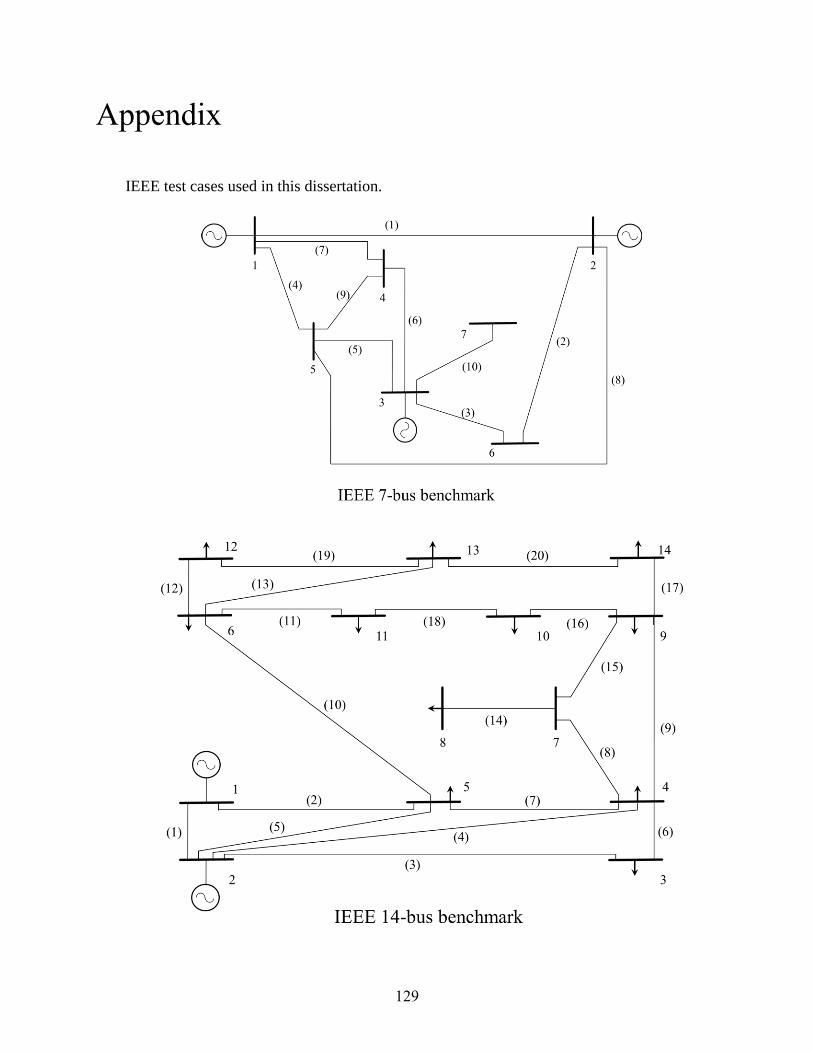
129
Appendix
IEEE test cases used in this dissertation.
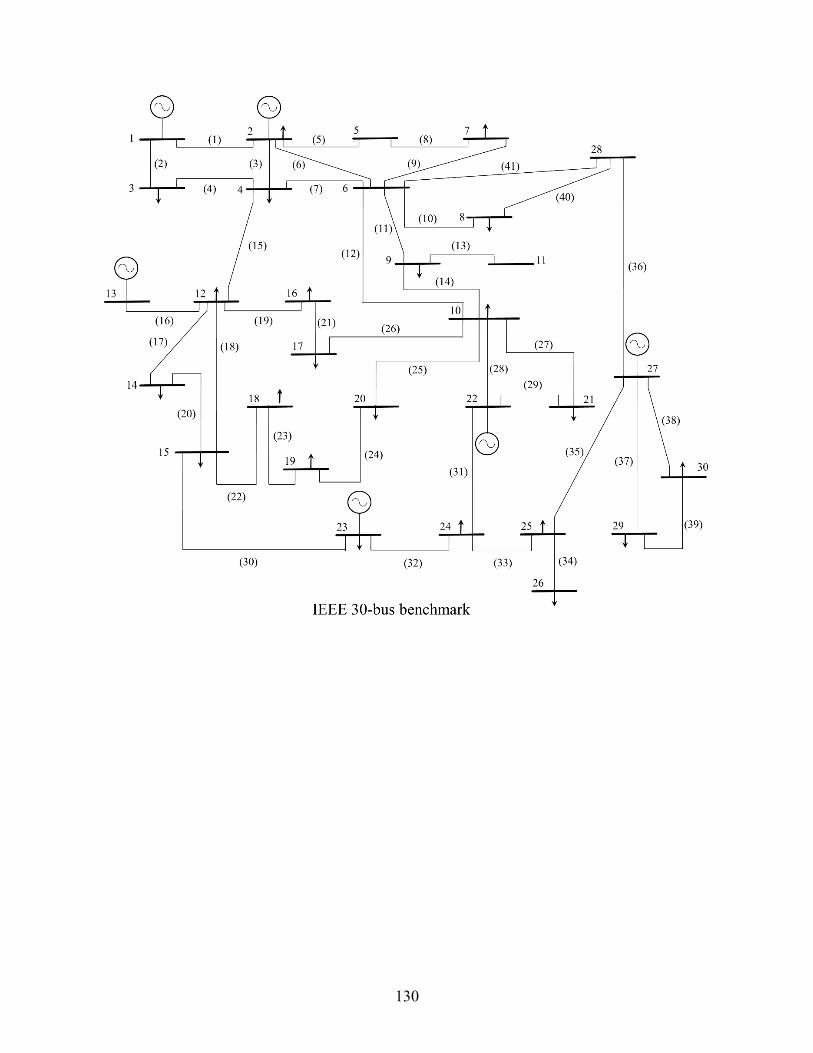
130

131
Vita
Pooria Mohammadi received his B.S. degree in electrical engineering from Iran University
of Science and Technology (IUST), Tehran, Iran, in 2010 and his M.S. degree focused in power
system and protection from University of Texas at Tyler, Texas, in 2013.
Currently, he is a Ph.D. candidate at the ECE department, Louisiana State University (LSU).
His current research includes power system protection, Optimal PMU Placement (OPP),
observability and state estimation, and Distributed Generations (DGs) integration. He has
conducted several projects for utility companies during his education and holds three patents. His
research interests also include smart grid, renewable energies, PMU applications, intelligent and
adaptive methods in power systems, and storage devices.