Programmable processors for wireless base-stations
Sridhar Rajagopal([email protected])
December 16, 2003

Wireless rates clock rates
Need to process 100X more bits per clock cycle today than in 1996
1996 1997 1998 1999 2000 2001 2002 2003 2004 2005 200610
-3
10-2
10-1
100
101
102
103
104
Year
Clock frequency (MHz)
W-LAN data rate (Mbps)
Cellular data rate (Mbps)
200 MHz
1 Mbps
9.6 Kbps
4 GHz
54-100 Mbps
2-10 Mbps

Base-stations need horsepower
Sophisticated signal processing for multiple users
Need 100-1000s of arithmetic operations to process 1 bit Base-stations require > 100 ALUs
‘Chip rate’processing
‘Symbol rate’processing
Decoding
‘Packet rate’processing
RF(Analog)
ASIC(s)and/or
ASSP(s)and/or
FPGA(s)
DSP(s)
Co-processor(s)and/or
ASIC(s)
DSP orRISC
processor

Programmable architectures
• Wireless algorithm kernels– Well known, ASIC mapping well-studied
• Processors getting more powerful every year
• Historic trend: ASICs Programmable
Can we design a fully programmable wireless system?

Thesis addresses the following problem
Design programmable processors for wireless base-stations with 100’s of ALUs :
(a)map wireless algorithms on these processors
(b)power-efficient (adapt resources to needs)(c) decide #ALUs, clock frequency
how much programmable? – as programmable as possible
Choice : Multi-processors
• Single processors won’t do– ILP, subword parallelism not sufficient– Register file explosion with increasing ALUs
• Multiprocessors– Data parallelism in wireless systems– Data-parallel/SIMD/vector processors appropriate
• Exploit ILP, MMX, DP

Thesis contributions
(a)Mapping algorithms on data-parallel processors – designing data-parallel algorithms– tradeoffs between packing, ALU utilization and memory– reduced inter-cluster communication network
(b)Improve power efficiency– adapting compute resources to workload variations – varying voltage and frequency to real-time requirements
(c) Design exploration between #ALUs and clock frequency to minimize power consumption– fast real-time performance prediction

Outline
• Background– Wireless systems– Data-parallel (Stream) processors
• Mapping algorithms to stream processors• Power efficiency • Design exploration
• Broad impact and future work

Wireless workloads
System 2G 3G 4G
UsersData ratesAlgorithmsEstimationDetection
DecodingTheoretical Min ALUs @ 1 GHz
32 16 Kbps /userSingle-user CorrelatorMatched filter
Viterbi> 2
32 128 Kbps/userMulti-userMax. likelihoodInterference CancellationViterbi> 20
321 Mbps/userMIMOChip equalizerMatched filter
LDPC> 200
Time1996 2003 ?
Key kernels studied for wireless
• FFT – Media processing• QRD – Media processing
• Outer product updates• Matrix – vector operations• matrix – matrix operations• Matrix transpose• Viterbi decoding• LDPC decoding (in progress)
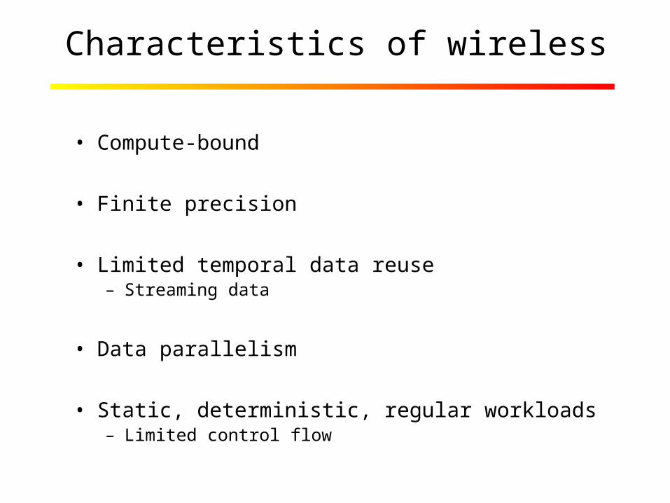
Characteristics of wireless
• Compute-bound
• Finite precision
• Limited temporal data reuse– Streaming data
• Data parallelism
• Static, deterministic, regular workloads– Limited control flow
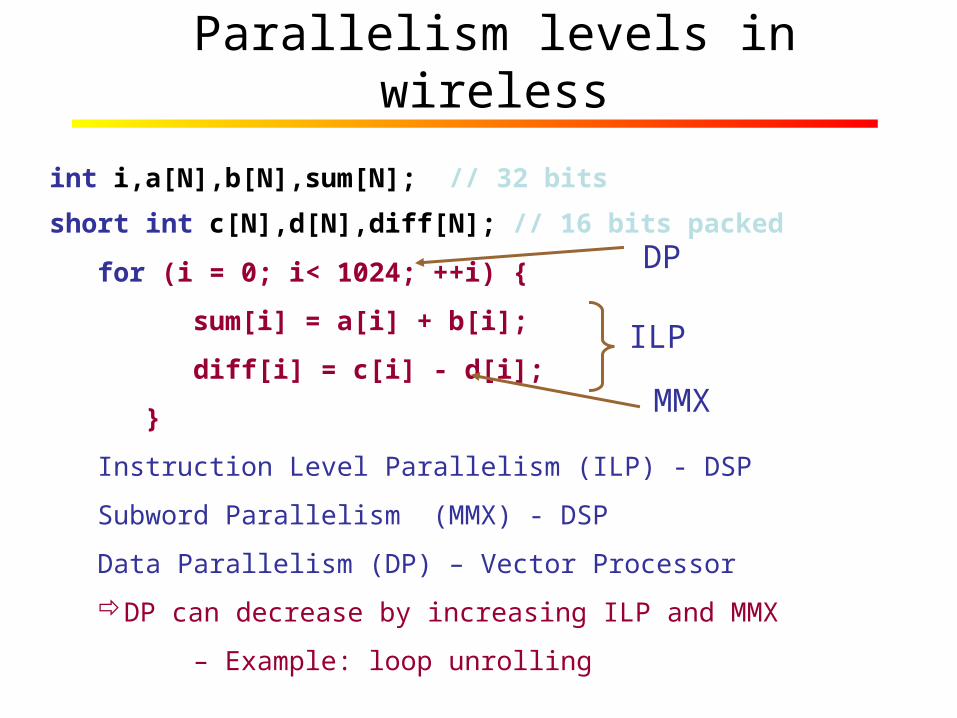
Parallelism levels in wireless
int i,a[N],b[N],sum[N]; // 32 bits
short int c[N],d[N],diff[N]; // 16 bits packed
for (i = 0; i< 1024; ++i) {
sum[i] = a[i] + b[i];
diff[i] = c[i] - d[i];
}
Instruction Level Parallelism (ILP) - DSP
Subword Parallelism (MMX) - DSP
Data Parallelism (DP) – Vector Processor
DP can decrease by increasing ILP and MMX
– Example: loop unrolling
ILP
DP
MMX
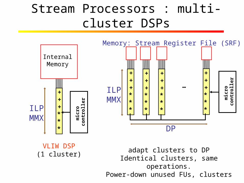
Stream Processors : multi-cluster DSPs
+++***
InternalMemory
ILPMMX
Memory: Stream Register File (SRF)
VLIW DSP(1 cluster)
+++***
+++***
+++***
+++***
…ILPMMX
DP
adapt clusters to DPIdentical clusters, same operations.Power-down unused FUs, clusters
mic
ro
con
tro
ller
mic
ro
con
tro
ller

Outline
• Background– Wireless systems– Stream processors
• Mapping algorithms to stream processors– Reduced inter-cluster communication network
• Power efficiency • Design exploration
• Broad impact and future work

Patterns in inter-cluster comm
• Intercluster comm network fully connected– Structure in access patterns can be exploited
• Broadcasting– Matrix-vector multiplication, matrix-matrix
multiplication, outer product updates
• Odd-even grouping– Transpose, Packing, Viterbi decoding
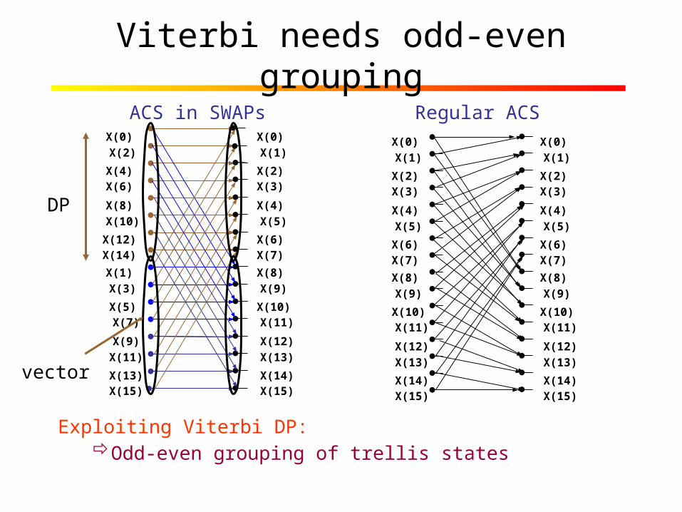
Viterbi needs odd-even grouping
Exploiting Viterbi DP:Odd-even grouping of trellis states
X(0)
X(1)
X(2)X(3)
X(4)
X(5)
X(6)X(7)
X(8)
X(9)
X(10) X(11)
X(12)
X(13)
X(14) X(15)
X(0)
X(1)
X(2)X(3)
X(4)
X(5)
X(6)X(7)
X(8)
X(9)
X(10) X(11)
X(12)
X(13)
X(14) X(15)
X(0)
X(2)
X(4)X(6)
X(8)
X(10)
X(12)X(14)
X(1)
X(3)
X(5) X(7)
X(9)
X(11)
X(13) X(15)
X(0)
X(1)
X(2)X(3)
X(4)
X(5)
X(6)X(7)
X(8)
X(9)
X(10) X(11)
X(12)
X(13)
X(14) X(15)
DP
vector
Regular ACSACS in SWAPs
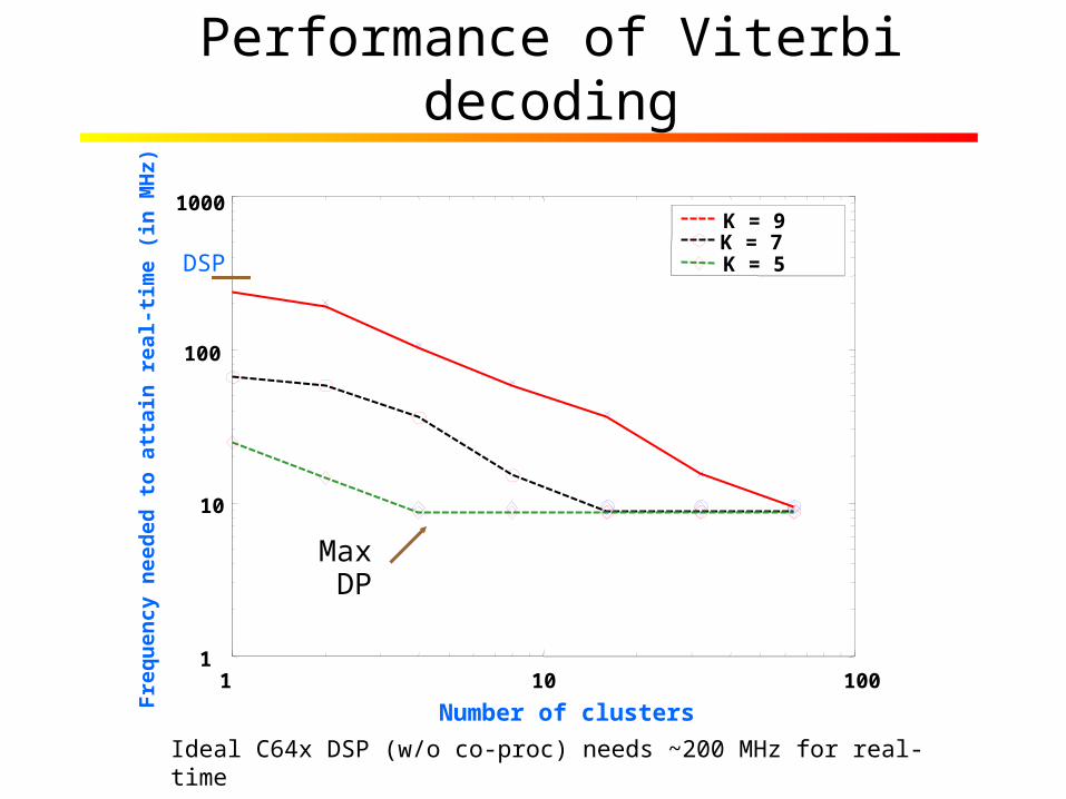
Performance of Viterbi decoding
Ideal C64x DSP (w/o co-proc) needs ~200 MHz for real-time
1 10 1001
10
100
1000
Number of clusters
Fre
qu
en
cy n
eed
ed
to a
ttain
real-
tim
e (
in M
Hz)
K = 9K = 7 K = 5DSP
Max DP

Odd-even grouping
• Packing– If odd-even data packed in same cluster and precision
doubles– Odd-even grouping required for bringing data to right
cluster– Not always beneficial for performance
• Matrix transpose– Better done in ALUs than in memory– Shown to have an order-of-magnitude better
performance – Done in ALUs as repeated odd-even groupings

Transpose uses odd-even grouping
N
M
0
M/2
1 2 3 4
A B C D
IN
OUT
Repeat LOG(M ) times{IN = OUT;}
A B C D
1 2 3 4C 3 D 4
A 1 B 2

Odd-even grouping
Inter-cluster communication
O(C2) wires, O(C 2) interconnections, 8 cycles
0/4 1/5 2/6 3/7
4 Clusters
Data
Entire chip lengthLimits clock frequencyLimits scaling
0 1 2 3 4 5 6 7 0 2 4 6 1 3 5 7
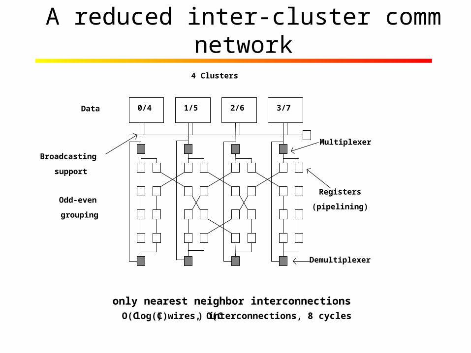
A reduced inter-cluster comm network
only nearest neighbor interconnectionsO(Clog(C)) wires, O(C) interconnections, 8 cycles
0/4 1/5 2/6 3/7
Broadcasting
support
Odd-even
grouping
Registers
(pipelining)
Multiplexer
4 Clusters
Demultiplexer
Data
Outline
• Background– Wireless systems– Stream processors
• Mapping algorithms to stream processors• Power efficiency • Design exploration
• Broad impact and future work
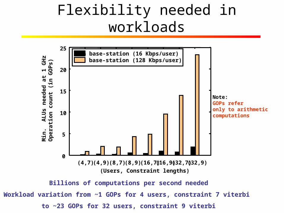
Flexibility needed in workloads
Billions of computations per second needed
Workload variation from ~1 GOPs for 4 users, constraint 7 viterbi
to ~23 GOPs for 32 users, constraint 9 viterbi
0
5
10
15
20
25
M
in.
AL
Us
nee
ded
at
1 G
Hz
Op
erat
ion
co
un
t (i
n G
OP
s)
(4,7) (4,9) (8,7) (8,9) (16,7) (16,9) (32,7) (32,9)
2G base-station (16 Kbps/user)3G base-station (128 Kbps/user)
(Users, Constraint lengths)
Note:GOPs referonly to arithmeticcomputations
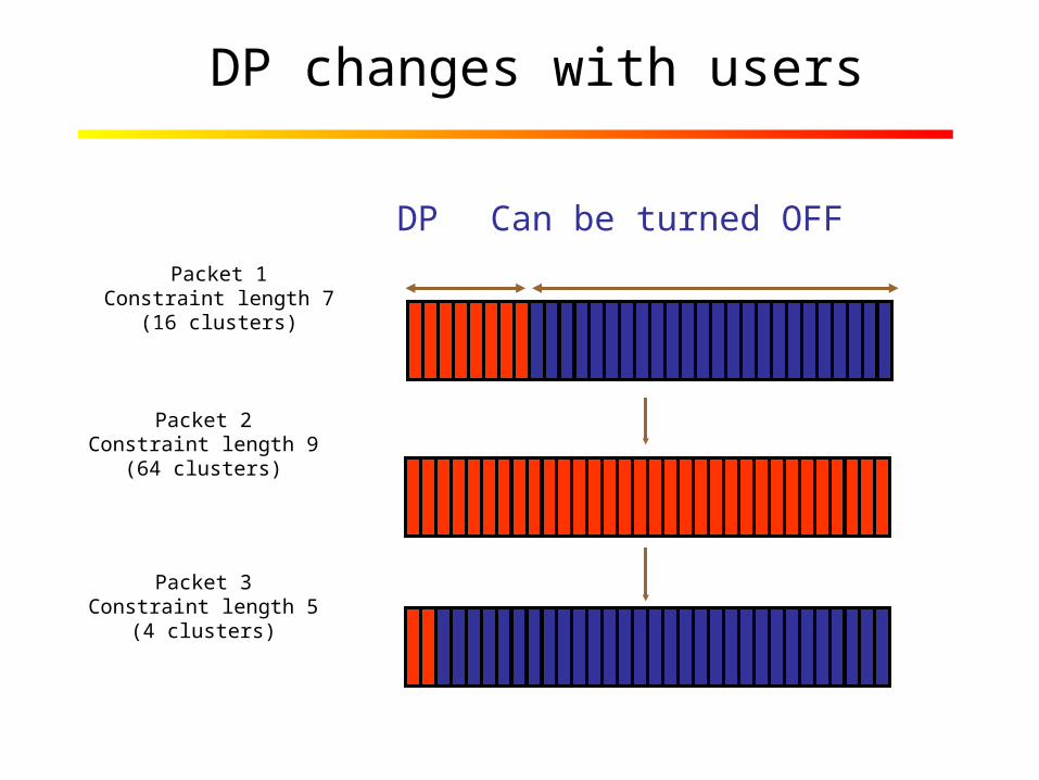
DP changes with users
Packet 1Constraint length 7
(16 clusters)
Packet 2Constraint length 9
(64 clusters)
Packet 3Constraint length 5
(4 clusters)
DP Can be turned OFF
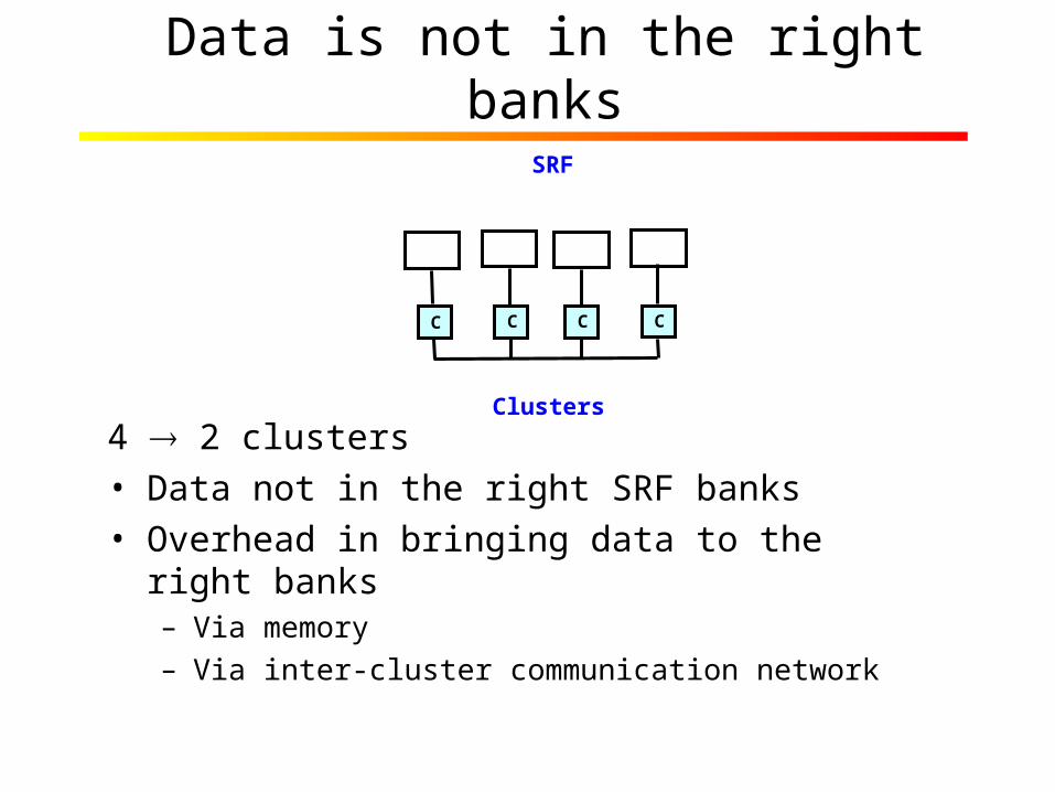
Data is not in the right banks
4 2 clusters• Data not in the right SRF banks• Overhead in bringing data to the right banks
– Via memory– Via inter-cluster communication network
C C C C
SRF
Clusters
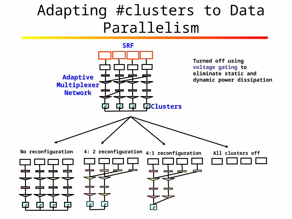
Adapting #clusters to Data Parallelism
AdaptiveMultiplexer
Network
C C C C
C C C C C CC
No reconfiguration 4: 2 reconfiguration 4:1 reconfiguration All clusters off
Turned off using voltage gating toeliminate static anddynamic power dissipation
SRF
Clusters
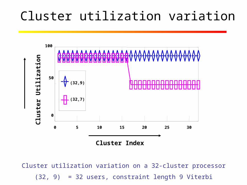
Cluster utilization variation
Cluster Index
0 5 10 15 20 25 30
0
50
100
(32,9)
(32,7)
Clu
ster
Uti
liza
tio
n
Cluster utilization variation on a 32-cluster processor
(32, 9) = 32 users, constraint length 9 Viterbi
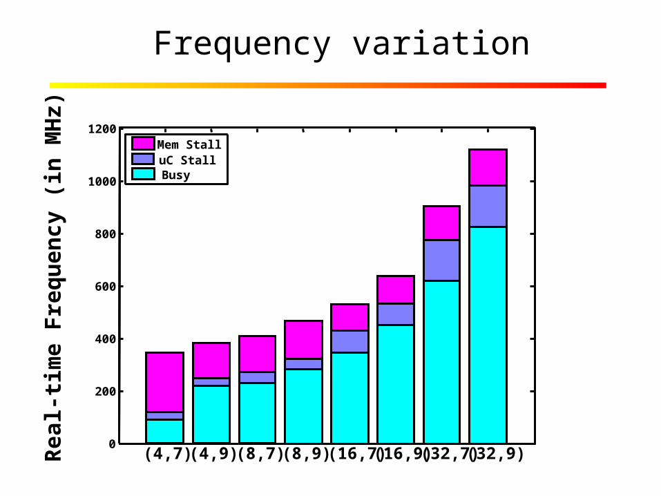
Frequency variation
0
200
400
600
800
1000
1200
Rea
l-ti
me
Fre
qu
ency
(in
MH
z)
(4,7) (4,9) (8,7) (8,9) (16,7) (16,9) (32,7) (32,9)
Mem StalluC Stall
Busy

Operation
• Dynamic Voltage-Frequency scaling when system changes significantly – Users, data rates …– Coarse time scale (when system changes)
• Turn off clusters – when parallelism changes – Finer time scale (once every 1000 cycles) (di/dt
effects)– Memory operations– Exceed real-time requirements
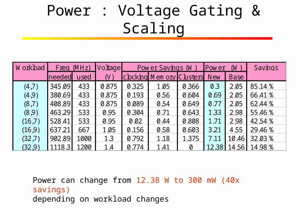
Power : Voltage Gating & Scaling
Workload Freq (MHz) Voltage Power Savings (W) Power (W) Savingsneeded used (V) clocking Memory Clusters New Base
(4,7) 345.09 433 0.875 0.325 1.05 0.366 0.3 2.05 85.14 %(4,9) 380.69 433 0.875 0.193 0.56 0.604 0.69 2.05 66.41 %(8,7) 408.89 433 0.875 0.089 0.54 0.649 0.77 2.05 62.44 %(8,9) 463.29 533 0.95 0.304 0.71 0.643 1.33 2.98 55.46 %(16,7) 528.41 533 0.95 0.02 0.44 0.808 1.71 2.98 42.54 %(16,9) 637.21 667 1.05 0.156 0.58 0.603 3.21 4.55 29.46 %(32,7) 902.89 1000 1.3 0.792 1.18 1.375 7.11 10.46 32.03 %(32,9) 1118.3 1200 1.4 0.774 1.41 0 12.38 14.56 14.98 %
Power can change from 12.38 W to 300 mW (40x savings) depending on workload changes

Outline
• Background– Wireless systems– Stream processors
• Mapping algorithms to stream processors• Power efficiency • Design exploration
• Broad impact and future work

Deciding ALUs vs. clock frequency
• No independent variables– Clusters, ALUs, frequency, voltage (c,a,m,f)– Trade-offs exist
• How to find the right combination for lowest power!
2P CV f V f 3P f
‘1’ cluster
100 GHz
(A)
+++***
‘a’+
‘m’*
+++***
‘a’+
‘m’*
+++***
‘a’+
‘m’*
‘c’ clusters
‘f’ MHz
+++***
‘1’+
‘1’*
+++***
‘10’+
‘10’*
+++***
‘10’+
‘10’*
+++***
‘10’+
‘10’*
‘100’ clusters
10 MHz
(B) (C)
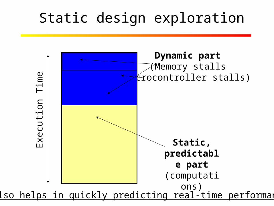
Static design exploration
also helps in quickly predicting real-time performance
Static, predictable
part(computations)
Dynamic part(Memory stalls
Microcontroller stalls)
Exe
cuti
on T
ime
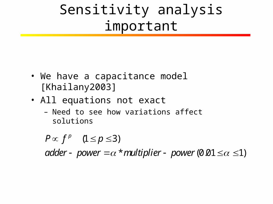
Sensitivity analysis important
• We have a capacitance model [Khailany2003]
• All equations not exact– Need to see how variations affect solutions
(1 3)
* (0.01 1)
pP f p
adder power multiplier power
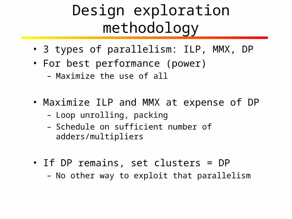
Design exploration methodology
• 3 types of parallelism: ILP, MMX, DP• For best performance (power)
– Maximize the use of all
• Maximize ILP and MMX at expense of DP– Loop unrolling, packing – Schedule on sufficient number of
adders/multipliers
• If DP remains, set clusters = DP– No other way to exploit that parallelism
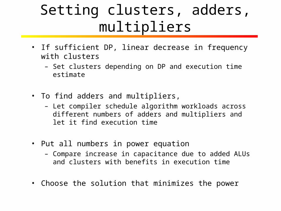
Setting clusters, adders, multipliers
• If sufficient DP, linear decrease in frequency with clusters– Set clusters depending on DP and execution time
estimate
• To find adders and multipliers,– Let compiler schedule algorithm workloads across
different numbers of adders and multipliers and let it find execution time
• Put all numbers in power equation– Compare increase in capacitance due to added ALUs
and clusters with benefits in execution time
• Choose the solution that minimizes the power
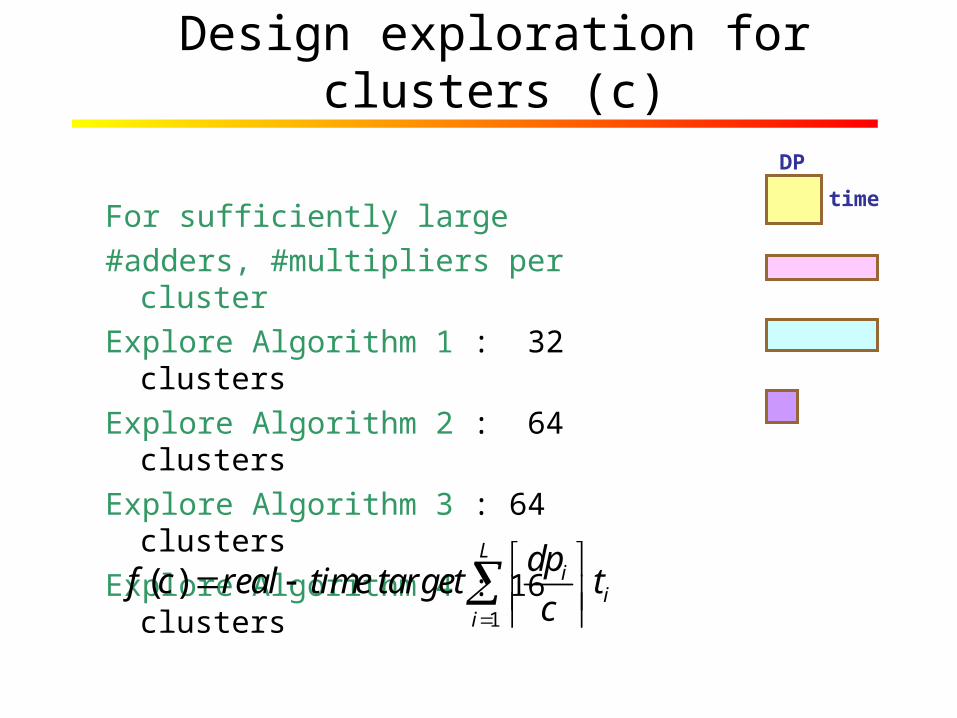
Design exploration for clusters (c)
For sufficiently large #adders, #multipliers per clusterExplore Algorithm 1 : 32 clusters Explore Algorithm 2 : 64 clusters Explore Algorithm 3 : 64 clusters Explore Algorithm 4 : 16 clusters
time
DP
1
( )L
ii
i
dpf c real time target t
c
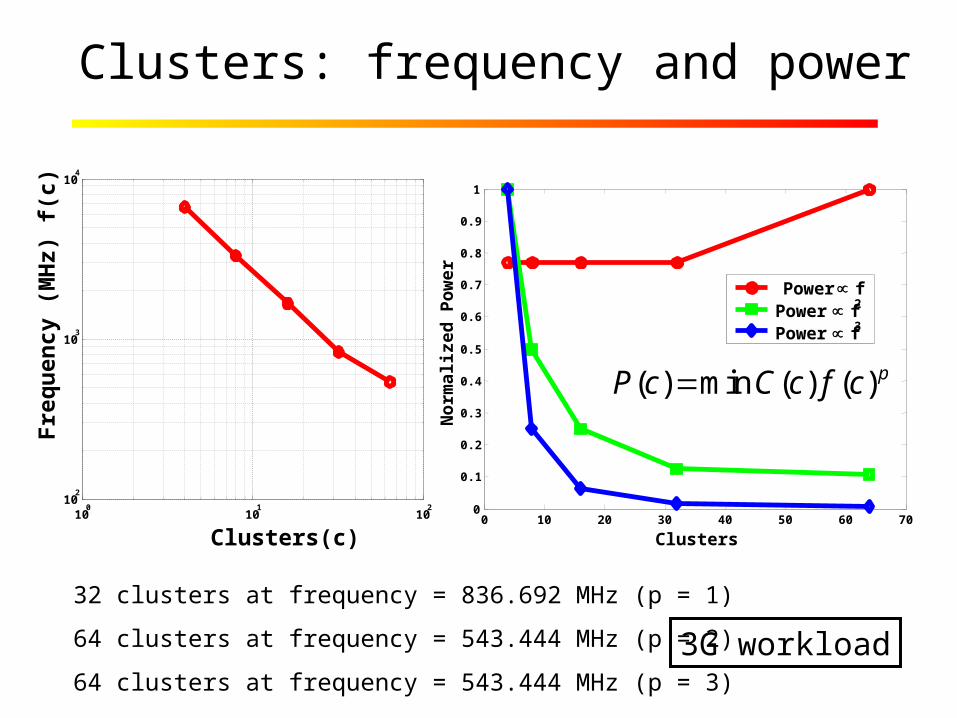
Clusters: frequency and power
100
101
102
102
103
104
Clusters(c)
Fre
qu
en
cy (
MH
z) f
(c)
0 10 20 30 40 50 60 700
0.1
0.2
0.3
0.4
0.5
0.6
0.7
0.8
0.9
1
Clusters
No
rmal
ized
Po
wer
Power fPower f2
Power f3
32 clusters at frequency = 836.692 MHz (p = 1)
64 clusters at frequency = 543.444 MHz (p = 2)
64 clusters at frequency = 543.444 MHz (p = 3)
( ) min ( ) ( ) pP c C c f c
3G workload
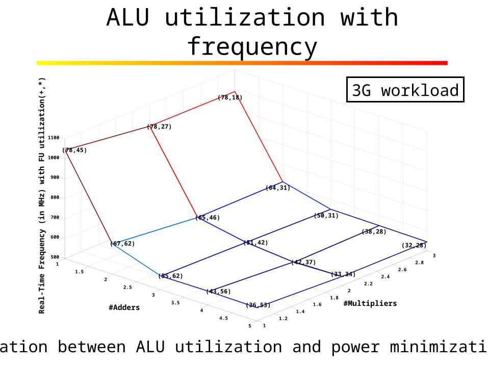
ALU utilization with frequency
3G workload
1
1.5
2
2.5
3
3.5
4
4.5
5 1
1.2
1.4
1.6
1.8
2
2.2
2.4
2.6
2.8
3500
600
700
800
900
1000
1100
(32,28)
(38,28)
#Multipliers
(33,34)
(50,31)
(42,37)
(64,31)
(36,53)
(51,42)
(78,18)
(43,56)
(65,46)
#Adders
(55,62)
(78,27)
(67,62)
(78,45)
Rea
l-T
ime
Fre
qu
ency
(in
MH
z) w
ith
FU
uti
liza
tio
n(+
,*)
Relation between ALU utilization and power minimization?

Choice of adders and multipliers
(,fp) Optimal Optimal ALU/Cluster Cluster/Total
Adders Multipliers Power Power
(0.01,1) 2 1 30 61
(0.01,2) 2 1 30 61
(0.01,3) 3 1 25 58
(0.1,1) 2 1 52 69
(0.1,2) 2 1 52 69
(0.1,3) 3 1 51 68
(1,1) 1 1 86 89
(1,2) 2 2 84 87
(1,3) 2 2 84 87

Exploration results
************************* Final Design Conclusion *************************Clusters : 64Multipliers/cluster : 1 Multiplier Utilization: 62%Adders/cluster : 3 Adder Utilization: 55%Real-time frequency : 568.68 MHz for 128
Kbps/user*************************
Exploration done in seconds….
Outline
• Background– Wireless systems– Stream processors
• Mapping algorithms to stream processors• Power efficiency • Design exploration
• Broad impact and future work

Broader impact
• Results not specific to base-stations– High performance, low power system designs
• Concepts can be extended to handsets
• Mux network applicable to all SIMD processors – Power efficiency in scientific computing
• Results #2, #3 applicable to all stream applications– Design and power efficiency– Multimedia, MPEG, …

Future work
Don’t believe the model is the reality
• Fabrication needed to verify concepts– Cycle accurate simulator – Extrapolating models for power
• LDPC decoding (in progress)– Sparse matrix requires permutations over large
data– Indexed SRF may help
• 3G requires 1 GHz at 128 Kbps/user– 4G equalization at 1 Mbps breaks down (expected)

Options for higher performance
• Multi-threading (ILP, MMX, DP, MT)– Schedule other kernels on unused clusters– Additional microcontroller and issue logic complexity
• Pipelining (ILP, MMX, DP, MT, PP)– Standard way of improving performance– Inter-processor communication overhead– Load-balancing difficult
• min(t1,t2,…) instead of min(t1+t2+,…)
• Software tools need to catch up with hardware

Need for new architectures, definitions and benchmarks
• Road ends - conventional architectures[Agarwal2000]
• Wide range of architectures – DSP, ASSP, ASIP, reconfigurable,stream, ASIC, programmable + – Difficult to compare and contrast– Need new definitions that allow comparisons
• Wireless workloads – Typically ASIC designs – SPEC benchmark needed for programmable designs

Conclusions
• Utilizing 100-1000s ALUs/clock cycle and mapping algorithms not easy in programmable architectures
• Data parallel algorithms need to be designed and mapped
• Power efficiency needs to be provided
• Design exploration needed to decide #ALUs to meet real-time constraints
– My thesis lays the initial foundations