Supporting Information
2D/2D Heterojunction of Ti3C2/g-C3N4 Nanosheets for Enhanced
Photocatalytic Hydrogen Evolution
Tongming Su,*a,b Zachary D. Hood,b,d Michael Naguib,c Lei Bai,b,f Si Luo,b Christopher M. Rouleau,b
Ilia N. Ivanov,b Hongbing Ji,a,e Zuzeng Qin,*a and Zili Wu*b
aSchool of Chemistry and Chemical Engineering, Guangxi University, Nanning 530004, China
bCenter for Nanophase Materials Sciences, Oak Ridge National Laboratory, Oak Ridge, Tennessee
37831, USA
cDepartment of Physics and Engineering Physics, Tulane University, New Orleans, Louisiana 70118,
USA
dElectrochemical Materials Laboratory, Department of Materials Science and Engineering,
Massachusetts Institute of Technology, Cambridge, Massachusetts 02139, USA
eSchool of Chemistry, Sun Yat-sen University, Guangzhou 510275, China
fWest Virginia University, Department of Chemical and Biomedical Engineering, Morgantown, West
Virginia 26506, USA
*Corresponding author: Tel: +1(865)576-1080.
E-mail: [email protected] (T. Su); [email protected] (Z. Qin); [email protected] (Z. Wu).
Electronic Supplementary Material (ESI) for Nanoscale.This journal is © The Royal Society of Chemistry 2019
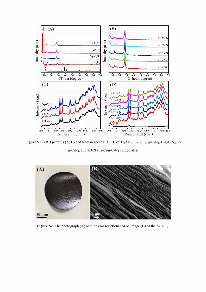
Figure S1. XRD patterns (A, B) and Raman spectra (C, D) of Ti3AlC2, S-Ti3C2, g-C3N4, B-g-C3N4, P-
g-C3N4, and 2D/2D Ti3C2/g-C3N4 composites.
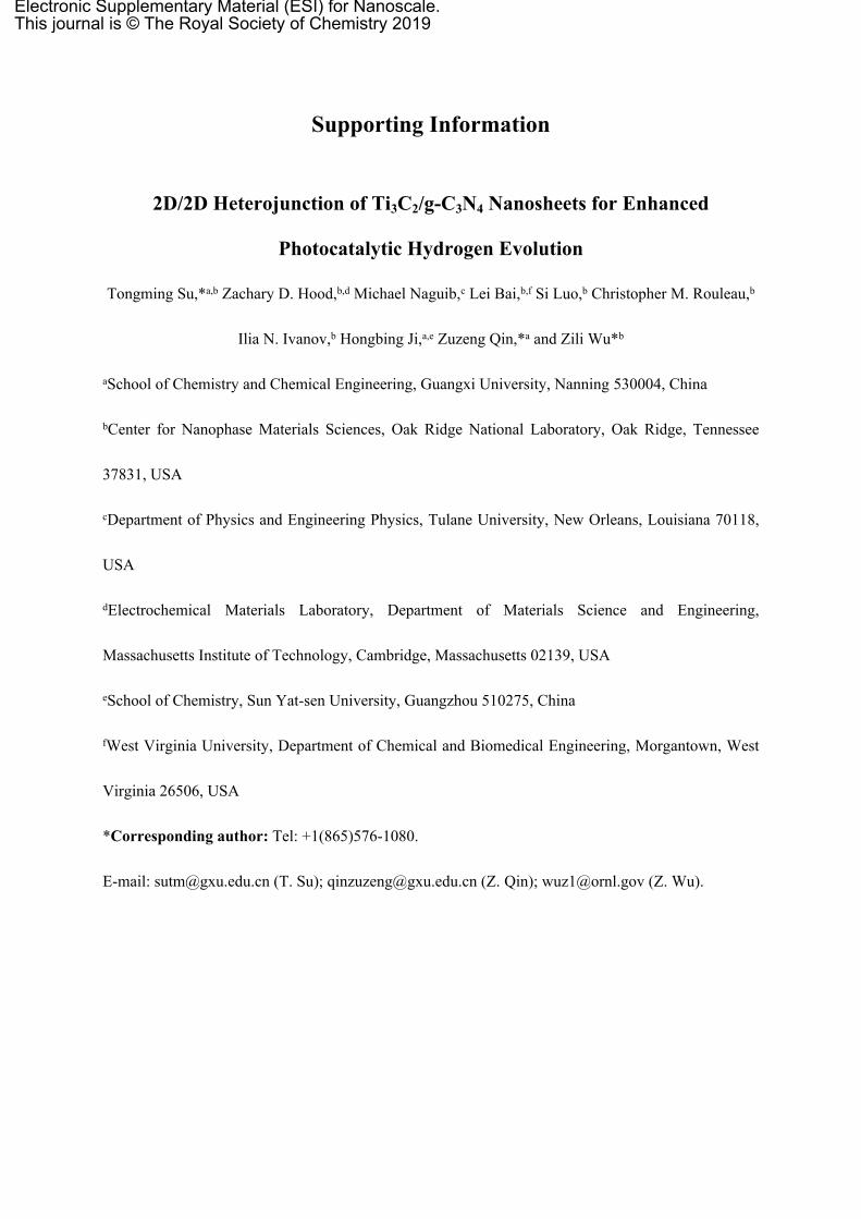
Figure S2. The photograph (A) and the cross-sectional SEM image (B) of the S-Ti3C2.
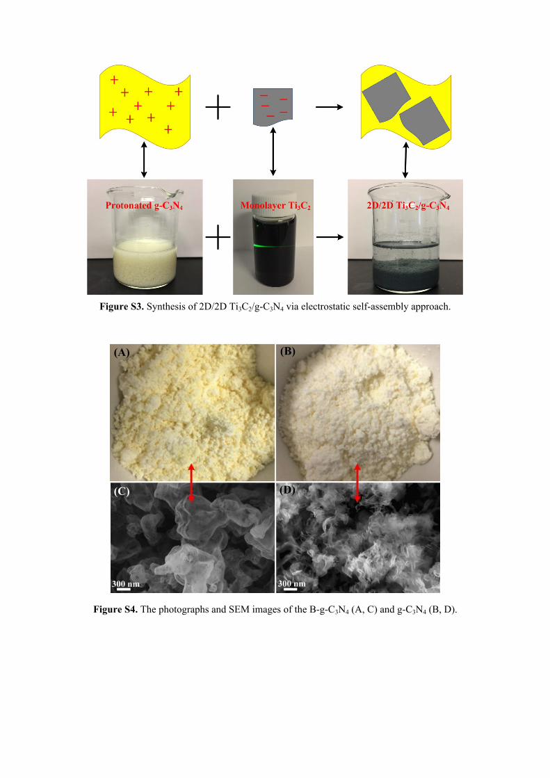
Figure S3. Synthesis of 2D/2D Ti3C2/g-C3N4 via electrostatic self-assembly approach.
Figure S4. The photographs and SEM images of the B-g-C3N4 (A, C) and g-C3N4 (B, D).

Figure S5. AFM height profile of a representative monolayer Ti3C2 deposited on Si wafer.
Figure S6. SEM image of Ti3AlC2 (A), photograph of the Ti3C2 flakes dispersion in water showing an
apparent Tyndall effect (B), AFM images (C) and thickness (D) of different Ti3C2 flakes.
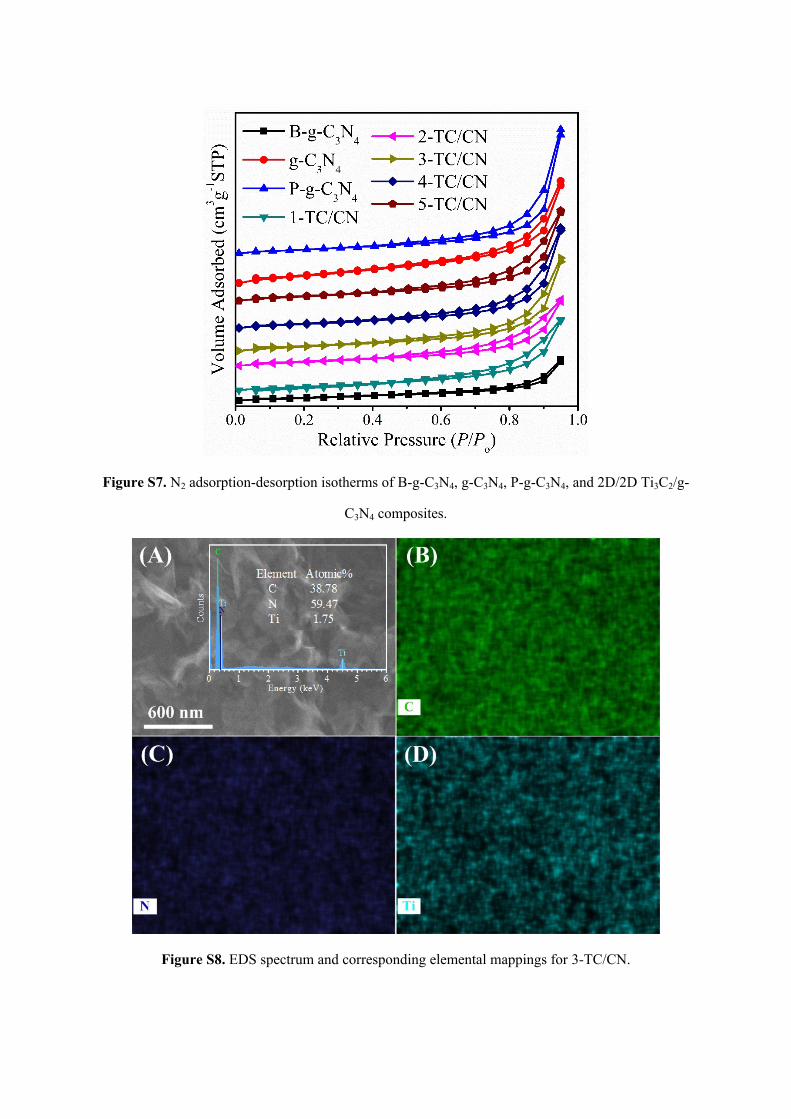
Figure S7. N2 adsorption-desorption isotherms of B-g-C3N4, g-C3N4, P-g-C3N4, and 2D/2D Ti3C2/g-
C3N4 composites.
Figure S8. EDS spectrum and corresponding elemental mappings for 3-TC/CN.
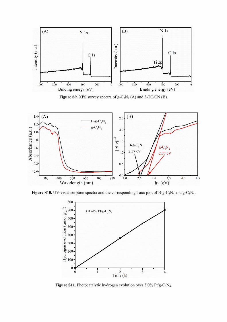
Figure S9. XPS survey spectra of g-C3N4 (A) and 3-TC/CN (B).
Figure S10. UV-vis absorption spectra and the corresponding Tauc plot of B-g-C3N4 and g-C3N4.
Figure S11. Photocatalytic hydrogen evolution over 3.0% Pt/g-C3N4.
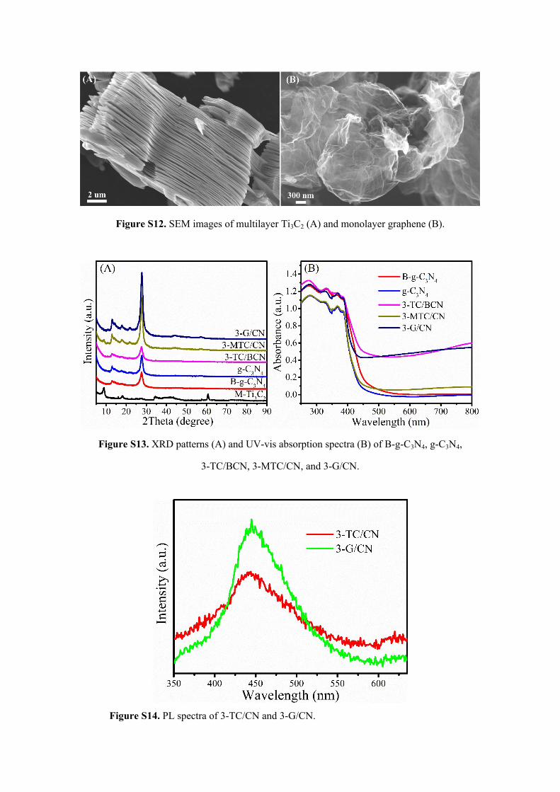
Figure S12. SEM images of multilayer Ti3C2 (A) and monolayer graphene (B).
Figure S13. XRD patterns (A) and UV-vis absorption spectra (B) of B-g-C3N4, g-C3N4,
3-TC/BCN, 3-MTC/CN, and 3-G/CN.
Figure S14. PL spectra of 3-TC/CN and 3-G/CN.
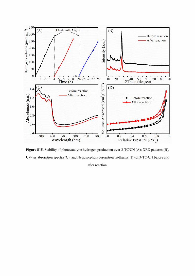
Figure S15. Stability of photocatalytic hydrogen production over 3-TC/CN (A); XRD patterns (B),
UV-vis absorption spectra (C), and N2 adsorption-desorption isotherms (D) of 3-TC/CN before and
after reaction.
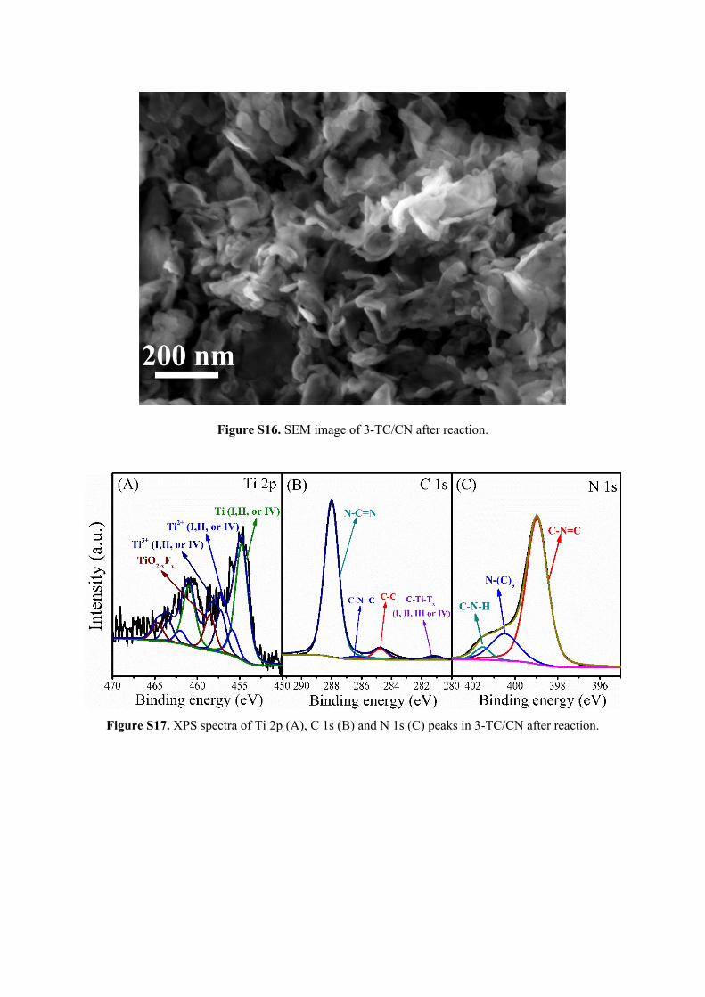
Figure S16. SEM image of 3-TC/CN after reaction.
Figure S17. XPS spectra of Ti 2p (A), C 1s (B) and N 1s (C) peaks in 3-TC/CN after reaction.
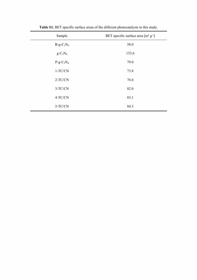
Table S1. BET specific surface areas of the different photocatalysts in this study.
Sample BET specific surface area [m2 g-1]
B-g-C3N4 58.0
g-C3N4 153.6
P-g-C3N4 79.0
1-TC/CN 73.8
2-TC/CN 76.6
3-TC/CN 82.0
4-TC/CN 83.1
5-TC/CN 84.3
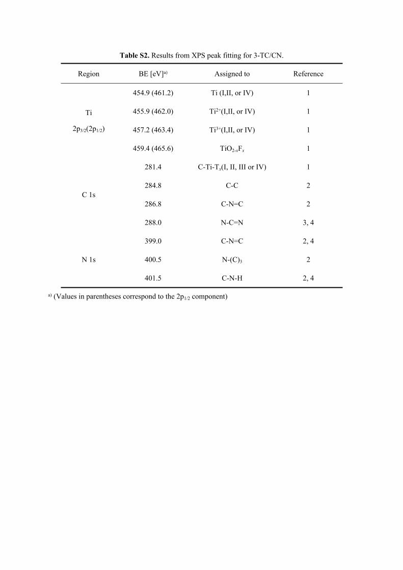
Table S2. Results from XPS peak fitting for 3-TC/CN.
Region BE [eV]a) Assigned to Reference
454.9 (461.2) Ti (I,II, or IV) 1
455.9 (462.0) Ti2+(I,II, or IV) 1
457.2 (463.4) Ti3+(I,II, or IV) 1
Ti
2p3/2(2p1/2)
459.4 (465.6) TiO2-xFx 1
281.4 C-Ti-Tx(I, II, III or IV) 1
284.8 C-C 2
286.8 C-N=C 2C 1s
288.0 N-C=N 3, 4
399.0 C-N=C 2, 4
400.5 N-(C)3 2N 1s
401.5 C-N-H 2, 4
a) (Values in parentheses correspond to the 2p1/2 component)
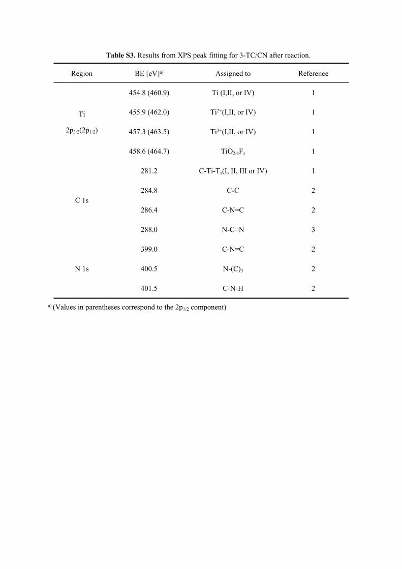
Table S3. Results from XPS peak fitting for 3-TC/CN after reaction.
Region BE [eV]a) Assigned to Reference
454.8 (460.9) Ti (I,II, or IV) 1
455.9 (462.0) Ti2+(I,II, or IV) 1
457.3 (463.5) Ti3+(I,II, or IV) 1
Ti
2p3/2(2p1/2)
458.6 (464.7) TiO2-xFx 1
281.2 C-Ti-Tx(I, II, III or IV) 1
284.8 C-C 2
286.4 C-N=C 2C 1s
288.0 N-C=N 3
399.0 C-N=C 2
400.5 N-(C)3 2N 1s
401.5 C-N-H 2
a) (Values in parentheses correspond to the 2p1/2 component)
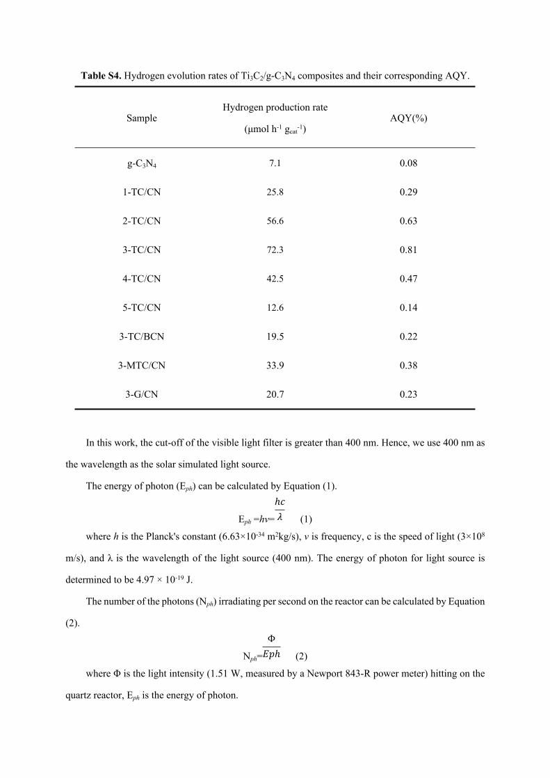
Table S4. Hydrogen evolution rates of Ti3C2/g-C3N4 composites and their corresponding AQY.
SampleHydrogen production rate
(μmol h-1 gcat-1)
AQY(%)
g-C3N4 7.1 0.08
1-TC/CN 25.8 0.29
2-TC/CN 56.6 0.63
3-TC/CN 72.3 0.81
4-TC/CN 42.5 0.47
5-TC/CN 12.6 0.14
3-TC/BCN 19.5 0.22
3-MTC/CN 33.9 0.38
3-G/CN 20.7 0.23
In this work, the cut-off of the visible light filter is greater than 400 nm. Hence, we use 400 nm as
the wavelength as the solar simulated light source.
The energy of photon (Eph) can be calculated by Equation (1).
Eph =hv= (1)
ℎ𝑐𝜆
where h is the Planck's constant (6.63×10⁻³⁴ m2kg/s), v is frequency, c is the speed of light (3×10⁸
m/s), and λ is the wavelength of the light source (400 nm). The energy of photon for light source is
determined to be 4.97 × 10⁻¹⁹ J.
The number of the photons (Nph) irradiating per second on the reactor can be calculated by Equation
(2).
Nph= (2)
Φ𝐸𝑝ℎ
where Φ is the light intensity (1.51 W, measured by a Newport 843-R power meter) hitting on the
quartz reactor, Eph is the energy of photon.
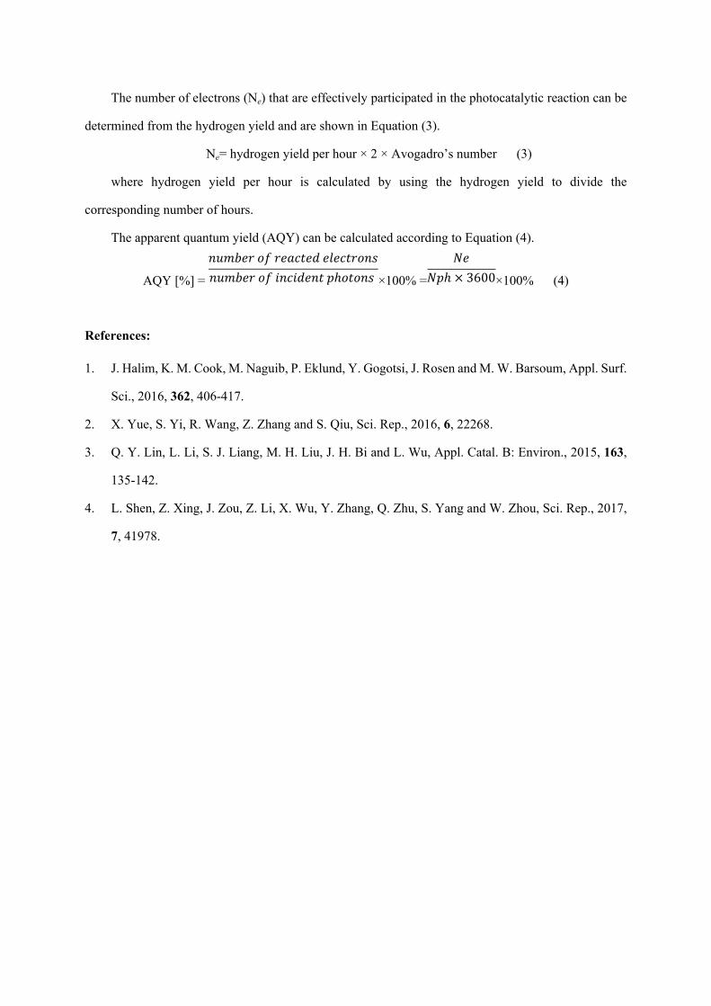
The number of electrons (Ne) that are effectively participated in the photocatalytic reaction can be
determined from the hydrogen yield and are shown in Equation (3).
Ne= hydrogen yield per hour × 2 × Avogadro’s number (3)
where hydrogen yield per hour is calculated by using the hydrogen yield to divide the
corresponding number of hours.
The apparent quantum yield (AQY) can be calculated according to Equation (4).
AQY [%] = ×100% = ×100% (4)
𝑛𝑢𝑚𝑏𝑒𝑟 𝑜𝑓 𝑟𝑒𝑎𝑐𝑡𝑒𝑑 𝑒𝑙𝑒𝑐𝑡𝑟𝑜𝑛𝑠𝑛𝑢𝑚𝑏𝑒𝑟 𝑜𝑓 𝑖𝑛𝑐𝑖𝑑𝑒𝑛𝑡 𝑝ℎ𝑜𝑡𝑜𝑛𝑠
𝑁𝑒𝑁𝑝ℎ × 3600
References:
1. J. Halim, K. M. Cook, M. Naguib, P. Eklund, Y. Gogotsi, J. Rosen and M. W. Barsoum, Appl. Surf.
Sci., 2016, 362, 406-417.
2. X. Yue, S. Yi, R. Wang, Z. Zhang and S. Qiu, Sci. Rep., 2016, 6, 22268.
3. Q. Y. Lin, L. Li, S. J. Liang, M. H. Liu, J. H. Bi and L. Wu, Appl. Catal. B: Environ., 2015, 163,
135-142.
4. L. Shen, Z. Xing, J. Zou, Z. Li, X. Wu, Y. Zhang, Q. Zhu, S. Yang and W. Zhou, Sci. Rep., 2017,
7, 41978.