Institut National des Sciences Appliquées de Rouen
Laboratoire d’Informatique de Traitement de l’Information et des Systèmes
Universitatea “Babeş-Bolyai”
Facultatea de Matematică şi Informatică, Departamentul de Informatică
P H D T H E S I S
Speciality : Computer Science
Defended by
Miron Alina Dana
to obtain the title of
Doctor of Computer Science of INSA de ROUEN
and “Babeş-Bolyai” University
Multi-modal, Multi-Domain Pedestrian Detection and Classification:
Proposals and Explorations in Visible over StereoVision, FIR and SWIR
16 July 2014
Jury :
Reviewers:
Fabrice Meriaudeau - Professor - “Bourgogne” University
Daniela Zaharie - Professor - “West” University of Timisoara
Crina Groşan - Associate Professor - “Babeş-Bolyai” University
Examiner:
Luc Brun - Professor - “Caen” University
PhD Directors:
Abdelaziz Bensrhair - Professor - INSA de Rouen
Horia F. Pop - Professor - “Babeş-Bolyai” University
PhD Supervisors:
Samia Ainouz - Associate Professor - INSA de Rouen
Alexandrina Rogozan - Associate Professor - INSA de Rouen


To Ovidiu, without whom
I would have never started this thesis
and to my family, that always
supported me


Acknowledgements
These are the voyages of my Phd. Its three-year mission (ok... four years in the end due to the
ATER): to explore strange new domains, to seek out new algorithms and new methods, to boldly
go where no man has gone before. The manuscript may not be as exciting as the board journal
of the Enterprise, but I thank the persons that will have the patience to read it. Also this thesis
would not exist without the help of several essential persons.
First of all, I would like to express my gratitude to my two Ph.D. directors, prof. Abdelaziz
Bensrhair and prof. Horia F. Pop, for their guidance. I could not have manage to do all this work
without the two Universities that hosted me during my thesis: INSA de Rouen in France, where
I’ve conducted almost all my activity, and “Babeş-Bolyai” University in Romania.
Second, I would like express my gratitude to the jury that accepted to review my thesis:
prof. Fabrice Meriaudeau (Université de Bourgogne), prof. Daniela Zaharie (West University of
Timisoara), Crina Groşan (“Babeş-Bolyai” University) and Luc Brun (Cean University). This list
includes my supervision committee from “Babeş-Bolyai” University: prof. Gabriela Czibula, Mihai
Oltean and Crina Groşan, and from INSA de Rouen: Samia Ainouz and Alexandrina Rogozan.
I would like to particularly thank Alexandrina Rogozan, without whom I would have never
come to France, and Samia Ainouz for her continuous guidance and help for the past years, both
professionally and personally.
I’m also grateful for the financial support given by CoDrive project, but also the ATER
position that has allowed me to finish writing the manuscript.
I would like to thank also my fellow comrades, the PhD students with whom I have shared
ideas, anxieties and joy: Florian, Guillaume, Zacharie, Amnir, Yadu, Vanee, Rawia, Nadine,
Xilan, Fabian. Also a special thank to my dear friends, Andreea, Cristina, Roxana, Flavia that
had the patience to listen to me complain during these years. I hope I did not forget anyone (If I
did, I will buy them an ice cream).

Last, but not the least, I would like to thank my love, Ovidiu, and my family, Ioan, Valeria,
Dinu, Marius, who gave me the opportunity to follow my dreams and for their continuous
encouragement.
Un sincer mulţumesc,
Alina Miron

Summary
The main purpose of constructing Intelligent Vehicles is to increase the safety for all traffic
participants. The detection of pedestrians, as one of the most vulnerable category of road users,
is paramount for any Advance Driver Assistance System (ADAS). Although this topic has been
studied for almost fifty years, a perfect solution does not exist yet. This thesis focuses on several
aspects regarding pedestrian classification and detection, and has the objective of exploring and
comparing multiple light spectrums (Visible, ShortWave Infrared, Far Infrared) and modalities
(Intensity, Depth by Stereo Vision, Motion).
From the variety of images, the Far Infrared cameras (FIR), capable of measuring the
temperature of the scene, are particular interesting for detecting pedestrians. These will usually
have higher temperature than the surroundings. Due to the lack of suitable public datasets
containing Thermal images, we have acquired and annotated a database, that we will name RIFIR,
containing both Visible and Far-Infrared Images. This dataset has allowed us to compare the
performance of different state of the art features in the two domains. Moreover, we have proposed a
new feature adapted for FIR images, called Intensity Self Similarity (ISS). The ISS representation
is based on the relative intensity similarity between different sub-blocks within a pedestrian region
of interest. The experiments performed on different image sequences have showed that, in general,
FIR spectrum has a better performance than the Visible domain. Nevertheless, the fusion of the
two domains provides the best results.
The second domain that we have studied is the Short Wave Infrared (SWIR), a light spectrum
that was never used before for the task of pedestrian classification and detection. Unlike FIR
cameras, SWIR cameras can image through the windshield, and thus be mounted in the vehicle’s
cabin. In addition, SWIR imagers can have the ability to see clear at long distances, making it
suitable for vehicle applications. We have acquired and annotated a database, that we will name
RISWIR, containing both Visible and SWIR images. This dataset has allowed us to compare the
performance of different pedestrian classification algorithms, along with a comparison between
Visible and SWIR. Our tests have showed that SWIR might be promising for ADAS applications,
performing better than the Visible domain on the considered dataset.
Even if FIR and SWIR have provided promising results, Visible domain is still widely used
due to the low cost of the cameras. The classical monocular imagers used for object detection
and classification can lead to a computational time well beyond real-time. Stereo Vision provides
a way of reducing the hypothesis search space through the use of depth information contained in
the disparity map. Therefore, a robust disparity map is essential in order to have good hypothesis
over the location of pedestrians. In this context, in order to compute the disparity map, we have
proposed different cost functions robust to radiometric distortions. Moreover, we have showed
that some simple post-processing techniques can have a great impact over the quality of the
obtained depth images.
The use of the disparity map is not strictly limited to the generation of hypothesis, and could
be used for some feature computation by providing complementary information to color images.
We have studied and compared the performance of features computed from different modalities
(Intensity, Depth and Flow) and in two domains (Visible and FIR). The results have showed that
the most robust systems are the ones that take into consideration all three modalities, especially
when dealing with occlusions.
Keywords: Intelligent Vehicles, Pedestrian Detection, Far-Infrared, Short-Wave Infrared,
StereoVision

Résumé
L’intérêt principal des systèmes d’aide à la conduite (ADAS) est d’accroître la sécurité de tous les
usagers de la route. Le domaine du véhicule intelligent porte une attention particulière au piéton,
l’une des catégories la plus vulnérable. Bien que ce sujet ait été étudié pendant près de cinquante
ans par des chercheurs, une solution parfaite n’existe pas encore. Nous avons exploré dans ce
travail de thèse différents aspects de la détection et la classification du piéton. Plusieurs domaines
du spectre (Visible, Infrarouge proche, Infrarouge lointain et stéréovision) ont été explorés et
comparés.
Parmi la multitude des systèmes imageurs existants, les capteurs infrarouge lointain (FIR),
capables de capturer la température des différents objets, reste particulièrement intéressants
pour la détection de piétons. Les piétons ont, le plus souvent, une température plus élevée que
les autres objets. En raison du manque d’accessibilité publique aux bases de données d’images
thermiques, nous avons acquis et annoté une base de donnée, nommé RIFIR, contenant à la fois
des images dans le visible et dans l’infrarouge lointain. Cette base nous a permis de comparer
les performances de plusieurs attributs présentés dans l’état de l’art dans les deux domaines.
Nous avons proposé une méthode générant de nouvelles caractéristiques adaptées aux images FIR
appelées « Intensity Self Similarity (ISS) ». Cette nouvelle représentation est basée sur la similarité
relative des intensités entre différents sous-blocks dans la région d’intérêt contenant le piéton.
Appliquée sur différentes bases de données, cette méthode a montré que, d’une manière générale,
le spectre infrarouge donne de meilleures performances que le domaine du visible. Néanmoins, la
fusion des deux domaines semble beaucoup plus intéressante.
La deuxième modalité d’image à laquelle nous nous sommes intéressé est l’infrarouge très
proche (SWIR, Short Wave InfraRed). Contrairement aux caméras FIR, les caméras SWIR sont
capables de recevoir le signal même à travers le pare-brise d’un véhicule. Ce qui permet de les
embarquer dans l’habitacle du véhicule. De plus, les imageurs SWIR ont la capacité de capturer

une scène même à distance lointaine. Ce qui les rend plus appropriées aux applications liées
au véhicule intelligent. Dans le cadre de cette thèse, nous avons acquis et annoté une base de
données, nommé RISWIR, contenant des images dans le visible et dans le SWIR. Cette base a
permis une comparaison entre différents algorithmes de détection et de classification de piétons
et entre le visible et le SWIR. Nos expérimentations ont montré que les systèmes SWIR sont
prometteurs pour les ADAS. Les performances de ces systèmes semblent meilleures que celles du
domaine du visible.
Malgré les performances des domaines FIR et SWIR, le domaine du visible reste le plus utilisé
grâce à son bas coût. Les systèmes imageurs monoculaires classiques ont des difficultés à produire
une détection et classification de piétons en temps réel. Pour cela, nous avons l’information
profondeur (carte de disparité) obtenue par stéréovision afin de réduire l’espace d’hypothèses
dans l’étape de classification. Par conséquent, une carte de disparité relativement correcte est
indispensable pour mieux localiser le piéton. Dans ce contexte, une multitude de fonctions coût
ont été proposées, robustes aux distorsions radiométriques, pour le calcul de la carte de disparité.
La qualité de la carte de disparité, importante pour l’étape de classification, a été affinée par un
post traitement approprié aux scènes routières.
Les performances de différentes caractéristiques calculées pour différentes modalités (Intensité,
profondeur, flot optique) et domaines (Visible et FIR) ont été étudiées. Les résultats ont montré
que les systèmes les plus robustes sont ceux qui prennent en considération les trois modalités,
plus particulièrement aux occultations.
Mots-clés: Véhicules intelligents, Détection de Piétons, Infrarouge lointain, Infrarouge à ondes
courtes, Stéréo Vision

Rezumat
Scopul principal al construt, iei vehiculelor inteligente este de a cres,te nivelul de sigurant,ă pentru
tot, i participant, ii la trafic. Detect, ia pietoniilor, fiind una dintre categoriile cele mai vulnerabile în
trafic, este de o important,ă majoră pentru orice Sistem de Asistent,ă Avansată la Conducere (en:
Advance Driver Assistance System - ADAS ). Des, i acest domeniu a fost studiat de aproape cincizeci
de ani, nu există încă o solut, ie perfectă. Această lucrare se concentreză pe diverse aspecte legate
de detect, ia s, i clasificarea pietonilor, s, i are ca obiectiv explorarea si compararea diverselor domenii
(Vizibil, Infraros,u de Lungime Scurtă, Infraros,u de Lungime Lungă) s, i modalităt, i (Intensitate,
Disparitate, Flux Optic).
Din divesele tipuri de senzori, spectrul Infraros,u de lungime de unde lungă (en: FIR), capabil
de a detecta temperatura diverselor obiecte, este deosebit de interesant pentru detectarea pietonilor.
Aces,tia din urmă, vor avea de regulă o temperatură mai ridicată decât mediul înconjurător. Din
lipsa unor baze de date adecvate cu imagini rutiere FIR, am achizit, ionat s, i adnotat o bază de
date cu imagini din acest spectru de lumină, pe care o vom numi RIFIR, cont, inând imagini atât
în spectrul Visibil cât s, i FIR. Aceste imagini ne-au permis să comparăm performant,a diverselor
caracteristici calculate pe imagini în cele două domenii. In contextul imaginilor termice, am
propus o nouă caracteristică adaptată pentru imaginile FIR, numită Intensity Self Similarity
(ISS ). Reprezentarea ISS este bazată pe calculul unor similarităt, i de intensitate între sub-blocuri
din interiorul unei regiuni de interes. Experimentele realizate pe diverse baze de imagini au arătat
că în general, spectrul FIR are o performant,ă mai bună decât domeniul Vizibil. Cu toate acestea,
fuziunea celor două spectre de lumină a dat performant,ele cele mai bune.
După analiza domeniului FIR, am studiat un alt spectru Infraros,u, care nu a fost folosit până
acum pentru detect, ia s, i clasificarea pietonilor, Infraros,u de Lungime Scurtă (Short Wave Infrared
- SWIR). Spre deosebire de camerele FIR, cele SWIR au abilitatea de a vedea prin parbriz, prin
urmare pot fi montate în interiorul vehiculului. În plus, camerele SWIR au posibilitatea de a

vedea clar pe distant,e lungi, ceea ce le face convenabile pentru aplicat, ii ADAS. Am achizit, ionat
s, i adnotat o nouă bază de imagini, pe care o vom numi RISWIR, cont, inând imagini atât din
Vizibil cât s, i din SWIR. Testele realizate au arătat rezultate promit,ătoare pentru spectrul SWIR
folosit în aplicat, ii de tip ADAS, având rezultate mai bune decât spectrul Visibil pe imaginile
considerate.
Chiar dacă FIR s, i SWIR au dat rezultate favorabile, spectrul Visibil este încă domeniul cel
larg utilizat, în special din cauza costului scăzut al echipamentelor. Clasicele imagini monoculare
folosite pentru detect, ia s, i clasificarea de obiecte pot să dea un timp de procesare foarte lung.
Stereo-Viziunea oferă o modalitate de a reduce spat, iul de căutare al ipotezelor prin folosirea
informat, iei privind distant,a până la obiecte, dată de harta de disparitate. Prin urmare, o hartă de
disparitate robustă este esent, ială pentru a avea ipoteze relevante cu privire la locat, ia pietonilor.
În acest context, pentru calculul hart, ii de disparitate am propus câteva funct, ii de cost robuste
la distorsiuni radiometrice. În plus, am arătat că technici simple de post-procesare pot avea un
impact semnificativ asupra calităt, ii hărt, ii de disparitate.
Folosirea hărt, ii de disparitate nu este strict limitată la generarea de ipoteze, ci poate să fie
utilizată s, i pentru calcularea unor caracteristici, funizând informat, ii complementare imaginilor
color. În acest context, am studiat s, i comparat performant,a caracteristicilor calculate pe diverse
modalităt, i (Intensitate, Disparitate s, i Fluxul Optic) în diverse domenii (Visibil s, i FIR). Rezultatele
au arătat că cele mai robuste sisteme sunt cele care iau în considerare toate cele trei modalităt, i,
în special pentru rezolvarea ocluziunilor.
Cuvinte cheie: Vehicule Inteligente, Detect, ia pietonilor , Infraros,u, FIR, SWIR, Stereo-Viziune

Contents
Introduction 15
1 Preliminaries 21
1.1 Motivation . . . . . . . . . . . . . . . . . . . . . . . . . . . . . . . . . . . . . . . . 21
1.2 Sensor types . . . . . . . . . . . . . . . . . . . . . . . . . . . . . . . . . . . . . . . 23
1.3 A short review of Pedestrian Classification and Detection . . . . . . . . . . . . . 24
1.3.1 Preprocessing . . . . . . . . . . . . . . . . . . . . . . . . . . . . . . . . . . 27
1.3.2 Hypothesis generation . . . . . . . . . . . . . . . . . . . . . . . . . . . . . 27
1.3.3 Object Classification/Hypothesis refinement . . . . . . . . . . . . . . . . . 29
1.4 Features . . . . . . . . . . . . . . . . . . . . . . . . . . . . . . . . . . . . . . . . . 30
1.4.1 Histogram of Oriented Gradients (HOG) . . . . . . . . . . . . . . . . . . . 31
1.4.2 Local Binary Patterns (LBP) . . . . . . . . . . . . . . . . . . . . . . . . . 31
1.4.3 Local Gradient Patterns (LGP) . . . . . . . . . . . . . . . . . . . . . . . . 33
1.4.4 Color Self Similarity (CSS) . . . . . . . . . . . . . . . . . . . . . . . . . . 35
1.4.5 Haar wavelets . . . . . . . . . . . . . . . . . . . . . . . . . . . . . . . . . . 35
1.4.6 Disparity feature statistics (Mean Scaled Value Disparity) . . . . . . . . . 35
1.5 Conclusion . . . . . . . . . . . . . . . . . . . . . . . . . . . . . . . . . . . . . . . . 36
2 Pedestrian detection and classification in Far Infrared Spectrum 37
2.1 Related Work . . . . . . . . . . . . . . . . . . . . . . . . . . . . . . . . . . . . . . 38
2.2 Datasets . . . . . . . . . . . . . . . . . . . . . . . . . . . . . . . . . . . . . . . . . 40
2.2.1 Dataset ParmaTetravision . . . . . . . . . . . . . . . . . . . . . . . . . . . 41
2.2.2 Dataset RIFIR . . . . . . . . . . . . . . . . . . . . . . . . . . . . . . . . . 45
2.3 A new feature for pedestrian classification in infrared images: Intensity Self Similarity 47
1

2.4 A study on Visible and FIR . . . . . . . . . . . . . . . . . . . . . . . . . . . . . . 50
2.4.1 Preliminaries . . . . . . . . . . . . . . . . . . . . . . . . . . . . . . . . . . 51
2.4.2 Feature performance comparison on FIR images . . . . . . . . . . . . . . . 51
2.4.3 Feature performance comparison on Visible images . . . . . . . . . . . . . 53
2.4.4 Visible vs FIR . . . . . . . . . . . . . . . . . . . . . . . . . . . . . . . . . 53
2.4.5 Visible & FIR Fusion . . . . . . . . . . . . . . . . . . . . . . . . . . . . . . 54
2.5 Conclusions . . . . . . . . . . . . . . . . . . . . . . . . . . . . . . . . . . . . . . . 54
3 Pedestrian Detection and Classification in SWIR 57
3.1 Related work . . . . . . . . . . . . . . . . . . . . . . . . . . . . . . . . . . . . . . 58
3.2 SWIR Image Analysis . . . . . . . . . . . . . . . . . . . . . . . . . . . . . . . . . 58
3.3 Preliminary SWIR images evaluation for pedestrian detection . . . . . . . . . . . 60
3.3.1 Hardware equipment . . . . . . . . . . . . . . . . . . . . . . . . . . . . . . 60
3.3.2 Dataset overview . . . . . . . . . . . . . . . . . . . . . . . . . . . . . . . . 62
3.3.3 Experiments . . . . . . . . . . . . . . . . . . . . . . . . . . . . . . . . . . . 63
3.4 SWIR vs Visible . . . . . . . . . . . . . . . . . . . . . . . . . . . . . . . . . . . . 67
3.4.1 Hardware equipment . . . . . . . . . . . . . . . . . . . . . . . . . . . . . . 68
3.4.2 Dataset overview . . . . . . . . . . . . . . . . . . . . . . . . . . . . . . . . 69
3.4.3 Experiments . . . . . . . . . . . . . . . . . . . . . . . . . . . . . . . . . . . 72
3.4.4 Discussion . . . . . . . . . . . . . . . . . . . . . . . . . . . . . . . . . . . . 73
3.5 Conclusions . . . . . . . . . . . . . . . . . . . . . . . . . . . . . . . . . . . . . . . 77
4 Stereo vision for road scenes 79
4.1 Stereo Vision Principles . . . . . . . . . . . . . . . . . . . . . . . . . . . . . . . . 81
4.1.1 Pinhole camera . . . . . . . . . . . . . . . . . . . . . . . . . . . . . . . . . 81
4.1.2 Stereo vision fundamentals . . . . . . . . . . . . . . . . . . . . . . . . . . 82
4.1.3 Stereo matching Algorithms . . . . . . . . . . . . . . . . . . . . . . . . . . 85
4.2 Stereo Vision Datasets . . . . . . . . . . . . . . . . . . . . . . . . . . . . . . . . . 97
4.3 Cost functions . . . . . . . . . . . . . . . . . . . . . . . . . . . . . . . . . . . . . . 99
4.3.1 Related work . . . . . . . . . . . . . . . . . . . . . . . . . . . . . . . . . . 99
4.3.2 State of the art of matching costs . . . . . . . . . . . . . . . . . . . . . . . 100
4.3.3 Motivation: Radiometric distortions . . . . . . . . . . . . . . . . . . . . . 104
4.3.4 Contributions . . . . . . . . . . . . . . . . . . . . . . . . . . . . . . . . . . 105
4.3.5 Algorithm . . . . . . . . . . . . . . . . . . . . . . . . . . . . . . . . . . . . 108
4.3.6 Experiments . . . . . . . . . . . . . . . . . . . . . . . . . . . . . . . . . . . 109
2

4.3.7 Discussion . . . . . . . . . . . . . . . . . . . . . . . . . . . . . . . . . . . . 113
4.4 Choosing the right color space . . . . . . . . . . . . . . . . . . . . . . . . . . . . . 114
4.4.1 Related work . . . . . . . . . . . . . . . . . . . . . . . . . . . . . . . . . . 114
4.4.2 Experiments . . . . . . . . . . . . . . . . . . . . . . . . . . . . . . . . . . . 116
4.4.3 Discussion . . . . . . . . . . . . . . . . . . . . . . . . . . . . . . . . . . . . 118
4.5 Conclusion . . . . . . . . . . . . . . . . . . . . . . . . . . . . . . . . . . . . . . . . 118
5 Multi-modality Pedestrian Classification in Visible and FIR 121
5.1 Related work . . . . . . . . . . . . . . . . . . . . . . . . . . . . . . . . . . . . . . 122
5.2 Overview and contributions . . . . . . . . . . . . . . . . . . . . . . . . . . . . . . 123
5.3 Datasets . . . . . . . . . . . . . . . . . . . . . . . . . . . . . . . . . . . . . . . . . 123
5.4 Preliminaries . . . . . . . . . . . . . . . . . . . . . . . . . . . . . . . . . . . . . . 125
5.5 Multi-modality pedestrian classification in Visible Domain . . . . . . . . . . . . . 126
5.5.1 Individual feature classification . . . . . . . . . . . . . . . . . . . . . . . . 126
5.5.2 Feature-level fusion . . . . . . . . . . . . . . . . . . . . . . . . . . . . . . . 128
5.6 Stereo matching algorithm comparison for pedestrian classification . . . . . . . . 134
5.7 Multi-modality pedestrian classification in Infrared and Visible Domains . . . . . 136
5.7.1 Individual feature classification . . . . . . . . . . . . . . . . . . . . . . . . 137
5.7.2 Feature-level fusion . . . . . . . . . . . . . . . . . . . . . . . . . . . . . . . 140
5.8 Conclusions . . . . . . . . . . . . . . . . . . . . . . . . . . . . . . . . . . . . . . . 140
6 Conclusion 141
A Comparison of Color Spaces 143
B Parameters algorithms stereo vision 147
C Disparity Map image examples 149
D Cost aggregation 151
E Voting-based disparity refinement 153
F Multi-modal pedestrian classification 155
F.1 Daimler-experiments - Occluded dataset . . . . . . . . . . . . . . . . . . . . . . . 155
Bibliography 159
3


List of Tables
1.1 Review of different camera types . . . . . . . . . . . . . . . . . . . . . . . . . . . 25
1.2 Review of other types of sensors . . . . . . . . . . . . . . . . . . . . . . . . . . . . 26
2.2 ParmaTetravision[Old] Dataset statistics . . . . . . . . . . . . . . . . . . . . . . . 41
2.1 Datasets comparison for pedestrian classification and detection in FIR images . . 42
2.3 ParmaTetravision Dataset statistics . . . . . . . . . . . . . . . . . . . . . . . . . . 43
2.4 Infrared Camera specification . . . . . . . . . . . . . . . . . . . . . . . . . . . . . 45
2.5 RIFIR Dataset statistics . . . . . . . . . . . . . . . . . . . . . . . . . . . . . . . . 46
2.6 Classification results with early fusion of ISS and HOG features FIR images on
ParmaTetravision[Old] . . . . . . . . . . . . . . . . . . . . . . . . . . . . . . . . . 50
3.1 Camera specifications . . . . . . . . . . . . . . . . . . . . . . . . . . . . . . . . . 61
3.2 Number of full-frame images on each tested bandwidth . . . . . . . . . . . . . . . 63
3.3 Results of HOG classifier on BB . . . . . . . . . . . . . . . . . . . . . . . . . . . . 64
3.4 Classifier Comparison in terms of Precision (P) and Recall (R) on SWIR images
over all the images . . . . . . . . . . . . . . . . . . . . . . . . . . . . . . . . . . . 65
3.5 Camera specification . . . . . . . . . . . . . . . . . . . . . . . . . . . . . . . . . . 68
3.6 RISWIR Dataset statistics . . . . . . . . . . . . . . . . . . . . . . . . . . . . . . . 69
4.1 Datasets comparison for stereo matching evaluation . . . . . . . . . . . . . . . . . 98
4.2 Error percentage of stereo matching with no aggregation (NoAggr) and window
aggregation (WAggr). . . . . . . . . . . . . . . . . . . . . . . . . . . . . . . . . . 110
4.4 Color Spaces used for comparison . . . . . . . . . . . . . . . . . . . . . . . . . . . 117
4.3 Average error . . . . . . . . . . . . . . . . . . . . . . . . . . . . . . . . . . . . . . 118
5.1 Datasets comparison for pedestrian classification and detection . . . . . . . . . . 124
5

LIST OF TABLES LIST OF TABLES
5.2 Training and test set statistics for Daimler Multi-Cue Dataset . . . . . . . . . . . 126
A.1 Color space comparison using No Aggregation and a Winner takes it all
strategy. . . . . . . . . . . . . . . . . . . . . . . . . . . . . . . . . . . . . . . . . 143
A.2 Color space comparison using No Aggregation and Window Voting strategy. 143
A.3 Color space comparison using No Aggregation and Cross Voting strategy. . 144
A.4 Color space comparison using Window Aggregation and Winner take it all
strategy. . . . . . . . . . . . . . . . . . . . . . . . . . . . . . . . . . . . . . . . . 144
A.5 Color space comparison using Window Aggregation and Window Voting
strategy. . . . . . . . . . . . . . . . . . . . . . . . . . . . . . . . . . . . . . . . . 144
A.6 Color space comparison using Window Aggregation and Cross Voting strategy.145
A.7 Color space comparison using Cross Aggregation and Winner Takes it all
strategy. . . . . . . . . . . . . . . . . . . . . . . . . . . . . . . . . . . . . . . . . 145
A.8 Color space comparison using Cross Aggregation and Window Voting strategy.145
A.9 Color space comparison using Cross Aggregation and Cross Voting strategy. 146
B.1 Parameters Algorithms Graph Cuts . . . . . . . . . . . . . . . . . . . . . . . . . . 147
B.2 Parameters Algorithms Cross Zone Aggregation . . . . . . . . . . . . . . . . . . . 147
E.1 Comparison of different strategy methods for choosing the disparity . . . . . . . . 154
6

List of Figures
1 Thesis structure . . . . . . . . . . . . . . . . . . . . . . . . . . . . . . . . . . . . . 18
2 Domain-modality-feature relationship . . . . . . . . . . . . . . . . . . . . . . . . . 18
1.1 Road traffic casualties by type of road user . . . . . . . . . . . . . . . . . . . . . 22
1.2 Causes by percentage of road accidents (in USA and Great Britain) . . . . . . . . 23
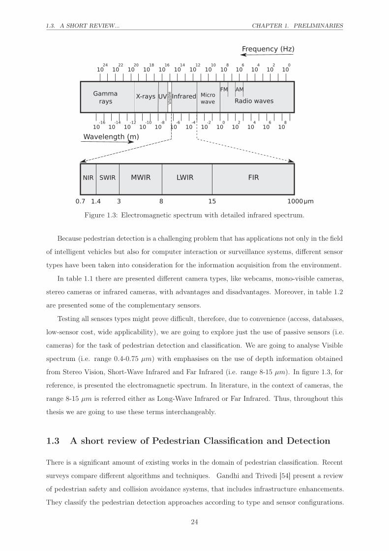
1.3 Electromagnetic spectrum with detailed infrared spectrum. . . . . . . . . . . . . 24
1.4 A simplified example of architecture for pedestrian detection . . . . . . . . . . . . 28
1.5 For a SVM trained on two-class problem, it is shown the maximum-margin hyper-
plane (along with the margins) . . . . . . . . . . . . . . . . . . . . . . . . . . . . 30
1.6 A pyramid as seen from two points of view . . . . . . . . . . . . . . . . . . . . . . 30
1.7 HOG Feature computation . . . . . . . . . . . . . . . . . . . . . . . . . . . . . . . 32
1.8 Examples of neighbourhood used to calculate a local binary pattern, where p are
the number of pixels in the neighbourhood, and r is the neighbourhood radius . . 33
1.9 Local binary pattern computation for a given pixel. In this example the pixel for
which the computation is performed is the central pixel having the intensity value 88. 34
1.10 Examples of Uniform (a) and non-uniform patterns (b) corresponding for LBP
computed with r = 1 and p = 8. There exist a total of 58 uniform local binarry
pattern plus one(for others) . . . . . . . . . . . . . . . . . . . . . . . . . . . . . . 34
1.11 Local gradient pattern operator computed for the central pixel having the intensity
88. . . . . . . . . . . . . . . . . . . . . . . . . . . . . . . . . . . . . . . . . . . . . 35
1.12 Haar wavelets a),b),c) and Haar-like features d),e). The sum of intensities in the
white area will be subtracted from the sum of intensities of the black area. . . . . 36
2.1 Images examples from Oldemera dataset a),b) . . . . . . . . . . . . . . . . . . . 41
2.2 Heat map of training for ParmaTetravision Dataset: a) Visible b) FIR . . . . . . 44
7

LIST OF FIGURES LIST OF FIGURES
2.3 Pedestrian height distribution of training (a) and testing (b) sets for ParmaTetravision 44
2.4 Images examples from ParmaTetravision dataset a) Visible spectrum b) Far-infrared
spectrum . . . . . . . . . . . . . . . . . . . . . . . . . . . . . . . . . . . . . . . . 44
2.5 Pedestrian height distribution of training (a) and testing sets (b) for RIFIR . . . 46
2.6 Heat map of training for RIFIR Dataset: a) Visible, b) FIR . . . . . . . . . . . . 47
2.7 Images examples from RIFIR dataset a) Visible spectrum b) Far-infrared spectrum 47
2.8 Visualisation of Intensity Self Similarity using histogram difference computed at
positions marked with blue in the IR images. A brighter cell shows a higher degree
of similarity. . . . . . . . . . . . . . . . . . . . . . . . . . . . . . . . . . . . . . . . 48
2.9 Performance of ISS feature on the dataset ParmaTetravision[Old] using different
histogram comparison strategies . . . . . . . . . . . . . . . . . . . . . . . . . . . . 49
2.10 Comparison of performance in terms of F-measure for different combination of
Histogram Size and Blocks Size . . . . . . . . . . . . . . . . . . . . . . . . . . . . 50
2.11 Performance comparison for features HOG, LBP, LGP and ISS in the FIR spectrum
on datasets a) RIFIR b) ParmaTetravision c) Oldemera-classification. The reference
point is considered the obtained false positive rate for a classification rate of 90%.
In figure d) are also shown the results for Oldemera-classification but this time as
miss-rate vs false positive rate. In this case the reference point is the miss rate
obtained for a false positive rate of 10−4 . . . . . . . . . . . . . . . . . . . . . . . 52
2.12 Peformance comparison for the features HOG, LBP, LGP and ISS in the Visible
domain on datasets a) RIFIR, b) ParmaTetravision . . . . . . . . . . . . . . . . . 53
2.13 Performance comparison of features between Visible and FIR domains on: a), c),
e), g) RIFIR dataset; b), d), f), h) ParmaTetravision dataset . . . . . . . . . . . . 55
2.14 Individual feature fusion between Visible and FIR domain on a) RIFIR dataset b)
ParmaTetravison dataset . . . . . . . . . . . . . . . . . . . . . . . . . . . . . . . . 56
3.1 Indoor image examples of how clothing appears differently between visible [a, c]
and SWIR spectra [b, d]. Appearance in the SWIR is influenced by the materials
composition and dyeing process. . . . . . . . . . . . . . . . . . . . . . . . . . . . . 59
3.2 Images acquired outdoor: SWIR and visible bandwidths highlight similar features
both for pedestrian and background. . . . . . . . . . . . . . . . . . . . . . . . . . 59
3.3 SWIR 2WIDE_SENSE camera . . . . . . . . . . . . . . . . . . . . . . . . . . . . 62
3.4 a) The 4× 4 filter mask applied on the FPA. b) Filters F1, F2 and F4 transmission
bands. . . . . . . . . . . . . . . . . . . . . . . . . . . . . . . . . . . . . . . . . . . 62
3.5 Height distribution over the annotated pedestrians. . . . . . . . . . . . . . . . . . 63
8

LIST OF FIGURES LIST OF FIGURES
3.6 Image comparison between Visible range (a1), F2 filter range (a2) and F1 filter
range (a3) with the corresponding on-column visualization of HAAR wavelets:
diagonal (b1, b2, b3), horizontal (c1), (c2), (c3), vertical (d1), (d2), (d3) and Sobel
filter (e1), (e2), (e3). Due to negligible values of the HAAR wavelet features along
the diagonal direction, the corresponding images [b1, b2, b3] appear very dark. . 64
3.7 Image examples from the sequences showing similar scenes and corresponding
output results given by the grammar models: C filter range (a), (d), (g), F2 filter
range (b), (e), (h) and F1 filter range (c), (f), (i). False positives produced by the
algorithm are surrounded by red BB while true positives are in green BB. . . . . 66
3.8 Results comparison when testing on all the BB vs. BB surrounding pedestrians
over 80 px only. . . . . . . . . . . . . . . . . . . . . . . . . . . . . . . . . . . . . . 67
3.9 Height distribution for the Training Sequence . . . . . . . . . . . . . . . . . . . . 70
3.10 Height distribution for the Testing Sequence . . . . . . . . . . . . . . . . . . . . . 70
3.11 Heat map given by the annotated pedestrians across training/testing and
SWIR/visible. . . . . . . . . . . . . . . . . . . . . . . . . . . . . . . . . . . . . . . 71
3.12 Examples of images from the dataset: a),c) Visible domain and the corresponding
images from the SWIR domain b),d) . . . . . . . . . . . . . . . . . . . . . . . . . 72
3.13 Feature performance comparison in the Visible domain. The reference point is
considered the obtained false positive rate for a classification rate of 90%. . . . . 73
3.14 Comparison of feature fusion performance in Visible domain. The reference point:
classification rate of 90%. . . . . . . . . . . . . . . . . . . . . . . . . . . . . . . . 74
3.15 Feature performance comparison in SWIR domain. The reference point: classifica-
tion rate of 90%. . . . . . . . . . . . . . . . . . . . . . . . . . . . . . . . . . . . . 74
3.16 Comparison of feature fusion performance in SWIR domain. The reference point:
classification rate of 90%. . . . . . . . . . . . . . . . . . . . . . . . . . . . . . . . 75
3.17 Comparison of Domain fusion performance for different features. The reference
point: classification rate of 90%. . . . . . . . . . . . . . . . . . . . . . . . . . . . . 75
3.18 Comparison in performance of Domain and different feature fusion strategies. The
reference point: classification rate of 90%. . . . . . . . . . . . . . . . . . . . . . . 76
4.1 An object as seen by two cameras. Due to camera positioning the object can have
different appearance in the constructed images. The distance between the two
cameras is called a baseline, while the difference in projection of a 3D point scene
in each camera perspective represents the disparity. . . . . . . . . . . . . . . . . . 80
9

LIST OF FIGURES LIST OF FIGURES
4.2 Pinhole camera. With a single camera, we cannot distinguish the position of a
projected point (P) in the 3D space (L1). . . . . . . . . . . . . . . . . . . . . . . 81
4.3 Stereo cameras. If we are able to match two projection points in the images as
being the same, we can easily infer the position of the considered 3D point by
simply intersecting the two light rays (L1 and L2) . . . . . . . . . . . . . . . . . . 82
4.4 Basic steps of stereo matching algorithms assuming rectified images. a) The
problem of stereo matching is to find for each pixel in one image the correspondent
in the other image. b) For each pixel a cost is computed, in this example the cost
is represented by the difference in intensities. c) A cost aggregation represented by
a squared window of 3× 3 pixels. d) The disparity of a pixel is usually chosen to
be the one that will give the minimum cost. . . . . . . . . . . . . . . . . . . . . 84
4.5 Challenging situations in stereo vision. The images a)-h) are extracted from the
KITTI dataset[57], while the images i)-l) from HCI/Bosh Challenge [95]. The
left column represents the left image from a stereo pair, and the right column
the corresponding right image.: a)-b) Textureless area on the road caused by sun
reflection; c)-d) Sun glare on the windshield produces artefacts; e)-f) "Burned"
area in image where the white building continues with the sky region caused by
high contrast between two areas of the image; g)-h) Road tiles produce a repetitive
pattern in the images; i)-j) Night images provide fewer information; k)-l) Reflective
surfaces will often produce inaccurate disparity maps . . . . . . . . . . . . . . . . 86
4.6 Disadvantage of square window-based aggregation at disparity discontinuities. In
red is the pixel, and the square is the corresponding aggregation area. . . . . . . 88
4.7 Cross region construction: a) For each pixel four arms are chosen based on some
color and distance restrictions; b),c) The cross region of a pixel is constructed by
taking for each pixel situated on the vertical arm, its horizontal arm limits. . . . 91
4.8 Cross region cost aggregation is perfomed into two steps: first the cost in the
cross-region is aggregated horizontally b) and then vertically b) . . . . . . . . . . 91
4.9 Four connected grid . . . . . . . . . . . . . . . . . . . . . . . . . . . . . . . . . . 92
4.10 Tree example. If smoothness assumption is modeled as a tree instead of a four
connected grid, the solution could be computed using dynamic programming . . . 93
4.11 From four-connected grid to tree: Scanline based tree . . . . . . . . . . . . . . . 94
4.12 Simple Tree structures: Horizontal Tree and Vertical Tree . . . . . . . . . . . . . 95
10

LIST OF FIGURES LIST OF FIGURES
4.13 Example of a minimum cut in a graph. A cut is represented by all the edges that
lead from the source set to the sink set (as seen in red edges). The sum of these
edges represents the cost of the cut. . . . . . . . . . . . . . . . . . . . . . . . . . . 96
4.14 Graph cuts example on a scanline in stereo vision: a) without smoothness assump-
tion; b) modelling smoothness assumption . . . . . . . . . . . . . . . . . . . . . . 97
4.15 Graph Cuts applied to stereo vision algorithm. . . . . . . . . . . . . . . . . . . . 97
4.16 Census mask: a) Dense configuration of 7× 7 pixels b) Sparse configuration for
CT with window size of 13× 13 pixels and step 2 . . . . . . . . . . . . . . . . . . 103
4.17 The mean percentage of radiometric distortions over the absolute color differences
between corresponding pixels in KITTI, respectively Middlebury dataset . . . . . 104
4.18 Bit string construction where the arrows show comparison direction for a) CT:
‘100001111’, b) CCC: ‘00001111101111110100’ in dense configuration, c) CCC in a
sparse configuration . . . . . . . . . . . . . . . . . . . . . . . . . . . . . . . . . . 105
4.19 Computation time comparison between CT and CCC for different image sizes. In
the figure an image size of 36 ∗ 104 corresponds to an image of 600× 600 pixels.
For both CT and CCC we used a window of 9× 7 pixels, but CCC is computed
using a step of two. . . . . . . . . . . . . . . . . . . . . . . . . . . . . . . . . . . . 106
4.20 Computation time comparison between CT and CCC for different neighbourhood
sizes for an image of 1000× 1000 pixels. . . . . . . . . . . . . . . . . . . . . . . . 107
4.21 Cost function (CDiffCT ) sensitivity to different parameters values . . . . . . . . . 110
4.22 Mean error for each cost function using graph cuts stereo matching. . . . . . . 112
4.23 Mean error for each cost function using local cross aggregation stereo matching.112
4.24 Output error (logarithmic-scale) for different cost functions in presence of radio-
metric distortions . . . . . . . . . . . . . . . . . . . . . . . . . . . . . . . . . . . 114
4.25 Comparison between cost functions. On first row there are presented two left visible
images ( a1 and c1) from the KITTI dataset with the corresponding ground truth
disparity images ( b1 and d1 ). On the following lines are the output disparity
maps corresponding to different functions: on the first ( a2-a10) and third column
( b2-b10) the output obtained with the cross zone aggregation (CZA) algorithm,
while on columns two (b2-b10) and fourth (d2-d10) the output of the graph cuts
algorithm. Images a2-a10 and b2-b10 correspond to the disparity map computed
for image a1 while the images c2-c10 and d2-d10 correspond to the disparity map
computed for image c1. . . . . . . . . . . . . . . . . . . . . . . . . . . . . . . . . 115
5.1 Comparison of Mean Scaled Value Disparity and Mean Value Disparity Zero Mean 127
11

LIST OF FIGURES LIST OF FIGURES
5.3 Individual classification performance comparison of different features in the three
modalities: a) Intensity; b) Depth; c) Motion; d) Best feature on each modality . 128
5.2 Individual classification (intensity, depth, motion) performance of on non-occluded
Daimler dataset a) HOG; b) ISS; c) LBP; d) LGP; e) Haar Wavelets; f) MSVZM .
The reference point is considered the obtained false positive rate for a classification
rate of 90%. . . . . . . . . . . . . . . . . . . . . . . . . . . . . . . . . . . . . . . . 129
5.4 Individual classification (intensity, depth, motion) performance on the partial
occluded testing set of a) HOG; b) ISS; c) LBP; d) LGP; e) Haar Wavelets; f)
MSVZM . . . . . . . . . . . . . . . . . . . . . . . . . . . . . . . . . . . . . . . . 130
5.5 Classification performance comparison for each feature using different modality fu-
sion (Intensity+Motion; Depth+Motion; Intensity+Depth; Intensity+Depth+Flow)
and the best single modality for each feature: a) HOG; b) ISS; c) LBP; d) LGP; e)
Haar Wavelets; f) MSVZM. . . . . . . . . . . . . . . . . . . . . . . . . . . . . . . 132
5.6 Classification performance comparison between different features using all modality
fusion per feature (a) along (b) with a comparison between the best feature
modality fusion (HOG on Intensity, Depth and Flow) and the best performing
feature on each modality ( HOG on Intensity, ISS on Depth and LGP computed
on Motion ) . . . . . . . . . . . . . . . . . . . . . . . . . . . . . . . . . . . . . . 133
5.7 Classification performance comparison between the fusion of best performing
feature on each modality ( HOG on Intensity, ISS on Depth and LGP on Motion
) with all modalities fusion of different features (HOG and LBP; HOG, ISS and
LBP; HOG, ISS and LGP; HOG, ISS, LBP and LGP) . . . . . . . . . . . . . . . 133
5.8 Classification performance comparison of three stereo matching algorithms from
the perspective of four features: a) HOG , b) ISS, c) LBP, d) LGP. . . . . . . . . 134
5.9 Classification performance comparison between different features (HOG, ISS, LGP,
LBP ) for Depth computed with three different stereo matching algorithms: a)
Local stereo matching using DiffCensus cost, b) Local stereo matching using
ADCensus cost, c) Stereo matching using the algorithm proposed by [56] . . . . 135
5.10 Individual classification (visible, depth, flow and IR) performance of a) HOG; b)
ISS; c) LBP; d) LGP; . . . . . . . . . . . . . . . . . . . . . . . . . . . . . . . . . 138
12

LIST OF FIGURES LIST OF FIGURES
5.11 Classification performance comparison for each feature using different modality
fusion (Visible+IR; Visible+Depth; IR+Depth; Intensity+Depth+IR) and the best
single modality for each feature: a) HOG; b) ISS; c) LBP; d) LGP. In order to
highlight differences between different features, in e) is plotted for comparison of
all modality fusion for different features. . . . . . . . . . . . . . . . . . . . . . . . 139
C.1 Comparison between cost functions. On first row there are presented the left visible
image number 0 ( a ) from the KITTI dataset with the corresponding ground truth
disparity ( b). On the following lines are the output obtained with the cross zone
aggregation (CZA) algorithm with two different functions: c) Census Tranform; d)
the proposed DiffCT . . . . . . . . . . . . . . . . . . . . . . . . . . . . . . . . . . 149
C.2 Comparison between cost functions. On first row there are presented the left visible
image number 2 ( a ) from the KITTI dataset with the corresponding ground truth
disparity ( b). On the following lines are the output obtained with the graph cuts
(GC) algorithm with two different functions: c) Census Tranform; d) the proposed
DiffCT . . . . . . . . . . . . . . . . . . . . . . . . . . . . . . . . . . . . . . . . . . 150
D.1 . . . . . . . . . . . . . . . . . . . . . . . . . . . . . . . . . . . . . . . . . . . . . . 151
D.2 Different cost aggregation strategies: a) Left Image; b) Disparity Ground Truth;
c) Disparity map computed using the strategy proposed by Zhang et al. [137]; d)
Disparity map computing using the strategy proposed by Mei et al. [93] . . . . . 152
E.1 Different Voting Strategies for the same image . . . . . . . . . . . . . . . . . . . . 154
F.1 Individual classification performance comparison of different features in the three
modalities for partially occluded testing set: a) Intensity; b) Depth; c) Motion; d)
Best feature on each modality . . . . . . . . . . . . . . . . . . . . . . . . . . . . . 155
F.2 Classification performance comparison for each feature using different modality
fusion on partially occluded testing set (Intensity+Motion; Depth+Motion;
Intensity+Depth; Intensity+Depth+Flow) and the best single modality for each
feature: a) HOG; b) ISS; c) LBP; d) LGP; e) Haar Wavelets; f) MSVZM. . . . . 156
F.3 Classification performance comparison on the partially occluded testing sets be-
tween different features using the best modality fusion per feature . . . . . . . . 157
F.4 Classification performance comparison on the partially occluded testing sets be-
tween different features using the all modality fusion per feature . . . . . . . . . 157
13


Your car should drive itself. It’s amazing to
me that we let humans drive cars. It’s a bug
that cars were invented before computers.
Eric Schmidt
Introduction
Intelligent autonomous vehicles have long surpassed the stage of a Sci-Fi idea, and have become
a reality [62],[1]. The main motivation behind this technology is to increase the safety of both
driver and other traffic participants. In this context, pedestrian protection systems have become
a necessity. But merely passive components like airbags are not enough: active safety, technology
assisting in the prevention of a crash, is vital. For this, a system of pedestrian detection and
classification plays a fundamental role.
Challenges
Pedestrian detection and classification in the context of intelligent vehicles in an urban environment
poses a lot of challenges:
Pedestrian Appearance and Shape. By nature, the humans have different heights and body
shapes. But this variability in appearance is further increased by different cloth types. Moreover,
human shape can change a lot in a short period of time (for example a person that bends to
tie its shoes). Also the appearance depends on the point of view of the camera, as well as the
distance between the camera and the pedestrian. Close pedestrians can bear little resemblance
with the ones situated far away.
Occlusion. Occlusions represents an important challenge for the detection of any type of object,
and in the case of pedestrians they can be divided into: self and external occlusions. Self-occlusion
are cause especially by the pose of the object, in the case of a pedestrian that has a side-way
position in relation with the point of view of the camera will certainly exhibit occlusion of some
body-parts. Moreover different objects carried by the pedestrians might have the same effect (for
example hats, bags, umbrellas). In the external occlusions category we include other pedestrians
15

LIST OF FIGURES LIST OF FIGURES
(especially in an urban situation), poles, other cars, as well as the situation in which the pedestrian
is too close to the camera leading certain body-parts exit the field of view.
Environmental conditions. Although some meteorological circumstances might not have a
direct impact on the quality of images (for example light rain), they can influence the appearance
of pedestrians for cameras (for example a passer-by can open an umbrella which might lead to
occlusion of the head region). Other conditions might lead to situations where the quality of
retrieved images is altered (for example situations of haze, fog, snow, heavy rain etc.). Another
factor that should be taken into consideration is the time of day, that has a direct impact over the
amount of ambient light available - usually, during daytime the problem of pedestrian detection
and classification poses less problems than during night.
Sensor choice. Each existing sensor has certain disadvantages and advantages, depending
on the situation. For example, passive sensors like visible cameras can be affected by low light
conditions, giving poor images with low variation in intensity across objects and background,
while thermal cameras might experience the same problems when the environment has a similar
temperature with the pedestrians. Active sensors, like LIDAR, have the advantage of providing
distance to all objects in a scene, but they have as output a large datasets that might be difficult
to interpret.
Other objects. Distinction between non-pedestrians and pedestrians might not be always
simple, being difficult to construct a model that differentiates between pedestrians and any other
existing objects.
Main Research Contributions
Motivated by the importance of pedestrian detection, there exist an extensive amount of work
done in connection with this field. Our objective is to study the problem across different light
spectrum and modalities, with an emphasis on disparity map.
Our main contributions can be summarised as follows:
• Creation and annotation of two databases for benchmarking of pedestrian classification,
one for Far-Infrared (FIR) and the other one in Short-Wave Infrared (SWIR).
• In the context of Thermal images, we have proposed a new feature, Intensity Self Similarity
(ISS). The performance of ISS was compared on three different datasets with state of the
art features.
16

LIST OF FIGURES LIST OF FIGURES
• As a novelty, we have studied the SWIR spectrum for the task of pedestrian classification,
and we have performed a comparison with the Visible domain.
• As a low cost solution, we believe that Stereo Vision is a promising alternative. In this
context, we have also focused on improving Stereo Matching algorithm by proposing new
cost functions.
• We have studied the performance of different features across different domains (Visible,
FIR) and across multiple modalities (Intensity, Motion, Disparity map)
Thesis Overview
This thesis is organized as follows (see also figure 1):
Chapter 1 presents an in-depth analysis for the motivation of a pedestrian detection system,
along with an overview of existing types of sensors. Our sensor of choice is passive sensors
represented by cameras sensitive to different light spectrums: Visible, Far Infrared and Short
Wave Infrared. We present also a short review of the steps employed in the task of pedestrian
classification and detection with an emphasise on the step of feature computation.
In Chapter 2 we study the problem of pedestrian classification in Thermal images (Far-
Infrared Spectrum). After overviewing existing datasets of Thermal images, we have reached
the conclusion that they all have important disadvantages: either the quality of the thermal
images is poor and there is not possibility of direct comparison with the Visible spectrum; or
the datasets are not publicly available. In this context, we have acquired and annotated a new
dataset. Moreover we have proposed a feature adapted for pedestrian classification in Far-Infrared
images and compared it with other state of the art features, in different conditions.
A new spectrum that can be interesting for the task of pedestrian detection and classification
is the Short-Wave Infrared (SWIR). An analysis of this light spectrum is made in Chapter 3.
After having performed some preliminaries experiments on a restricted dataset, we have acquired
and annotated a dataset of SWIR images, along with the Visible correspondent. On this later
dataset, we have compared the two spectrums from the perspective of different features.
Infrared cameras represent an interesting alternative to Visible cameras, and in general with
better results, but remains an expensive one. In this context, StereoVision could improve the
results obtained by just the employment of Visible cameras. Chapter 4 deals with the algorithms
of Stereo Matching. We propose several improvements for this algorithm, that mostly focus on
the employed cost function.
Chapter 5 treats the problem of multi-modality pedestrian classification (Intensity, Depth
17

LIST OF FIGURES LIST OF FIGURES
!"#$%&'(
)**
+),)+
!"#$%&'-
*.)+/01#23454
*.)+/64/754582&
!"#$%&'9
!!!
:5;;!&14<4
!=4%/,<1>%5=14/
01#23454
754582&/64/,)+
Figure 1: Thesis structure
Figure 2: Domain-modality-feature relationship
and Optical Flow) in both Visible and FIR spectrum. In figure 2 is presented the difference
between the domains and modalities employed. Moreover we show a preliminary analysis of the
impact of the quality of the Disparity Map over the results of classification. Finally, conclusions
and future work are presented in Chapter 6.
List of articles
Journal Papers
• Alina Miron, Samia Ainouz, Alexandrina Rogozan, Abdelaziz Bensrhair, "A robust cost
function for stereo matching of road scenes", Pattern Recognition Letters, No. 38, (2014):
70-77.
• Alina Miron, "Post Processing Voting Techniques for Local Stereo Matching", Studia Univ.
Babes-Bolyai, Informatica, Volume LIX, Number 1, (2014): 106-115
• Alina Miron, Samia Ainouz, Alexandrina Rogozan, Abdelaziz Bensrhair, "Cross-
comparison census for colour stereo matching applied to intelligent vehicle.", Electronics
18

LIST OF FIGURES LIST OF FIGURES
Letters 48.24 (2012): 1530-1532.
• Alina Miron, Samia Ainouz, Alexandrina Rogozan, Abdelaziz Bensrhair, Horia F.
Pop,"Stereo Matching Using radiometric Invariant measures", Studia Univ. Babes-Bolyai,
Informatica, Volume LVI, No.3, (2011): 91-96.
Conferences
• Fan Wang, Alina Miron, Samia Ainouz, Abdelaziz Bensrhair, Post-Aggregation Stereo
Matching Method using Dempster-Shafer Theory, IEEE International Conference on Image
Processing 2014 (accepted)
• Alina Miron, Rean Isabella Fedriga, Abdelaziz Bensrhair, and Alberto Broggi, SWIR
Images Evaluation for Pedestrian Detection in Clear Visibility Conditions, Proceedings of
IEEE ITSC (2013): 354-359
• Massimo Bertozzi, Rean Isabella Fedriga, Alina Miron, and Jean-Luc Reverchon, Pedes-
trian Detection in Poor Visibility Conditions: Would SWIR Help?, IEEE ICIAP (2013):
229-238
• Alina Miron, Bassem Besbes, Alexandrina Rogozan, Samia Ainouz, Abdelaziz Bensrhair,
Intensity Self Similarity Features for Pedestrian Detection in Far-Infrared Images, IEEE
Intelligent Vehicle Symposium (2012): 1120-1125
• Alina Miron, Samia Ainouz, Alexandrina Rogozan, Abdelaziz Bensrhair, Towards a
robust and fast color stereo matching for intelligent vehicle application, IEEE International
Conference on Image Processing (2012): 465-468
Presentations
• One Day BMVA Symposium at the British Computer Society: "Stereo Matching using
invariant radiometric features", London, May 18th 2011
• Journee GdR ISIS, Analyse de scenes urbaines en image et vision, "Stereo-vision for urban
scenes.", Nov. 8th 2012, Paris
19


Management by objective works - if you know
the objectives. Ninety percent of the time
you don’t.
Peter Drucker
1Preliminaries
Contents
1.1 Motivation . . . . . . . . . . . . . . . . . . . . . . . . . . . . . . . . . . 23
1.2 Sensor types . . . . . . . . . . . . . . . . . . . . . . . . . . . . . . . . . 25
1.3 A short review of Pedestrian Classification and Detection . . . . . . 26
1.3.1 Preprocessing . . . . . . . . . . . . . . . . . . . . . . . . . . . . . . . . . 29
1.3.2 Hypothesis generation . . . . . . . . . . . . . . . . . . . . . . . . . . . . 29
1.3.3 Object Classification/Hypothesis refinement . . . . . . . . . . . . . . . . 31
1.4 Features . . . . . . . . . . . . . . . . . . . . . . . . . . . . . . . . . . . . 32
1.4.1 Histogram of Oriented Gradients (HOG) . . . . . . . . . . . . . . . . . . 33
1.4.2 Local Binary Patterns (LBP) . . . . . . . . . . . . . . . . . . . . . . . . 33
1.4.3 Local Gradient Patterns (LGP) . . . . . . . . . . . . . . . . . . . . . . . 36
1.4.4 Color Self Similarity (CSS) . . . . . . . . . . . . . . . . . . . . . . . . . 37
1.4.5 Haar wavelets . . . . . . . . . . . . . . . . . . . . . . . . . . . . . . . . . 37
1.4.6 Disparity feature statistics (Mean Scaled Value Disparity) . . . . . . . . 37
1.5 Conclusion . . . . . . . . . . . . . . . . . . . . . . . . . . . . . . . . . . 38
1.1 Motivation
As shown in a report published by World Health Organization from 2013 [104], it is estimated
that every year 1.24 million people die as a result of a road traffic collision. That means that
over 3000 deaths occur each day. An additional 20 to 50 million1 more people sustain non-fatal
injuries from a collision, leading the traffic collision to be also one of the top causes of disability
worldwide.1Non-fatal crash injuries are insufficiently documented
21

1.1. MOTIVATION CHAPTER 1. PRELIMINARIES
Road traffic injuries are the eight leading cause of death globally, among the three leading
causes of death for people between 5 and 44 years of age and the first cause of death for people
aged 15− 19. Another sad statistic is that road crashes kill 260 000 children a year and injure
about 10 million (join report of Unicef and the World Health Organization). Without any action
taken, road traffic injuries are predicted to become the fifth leading cause of death in the world,
reaching around 2 million deaths per year by 2020. The main cause of the increase in number of
deaths is caused by a rapid increase in motorization without sufficient improvement in road safety
strategies and land use planning. The economic consequences of motor vehicle crashes have been
estimated between 1% and 3% of the respective GNP2 of the world countries, reaching a total
over $500 billion.
Analysing the casualties worldwide by the type of road user shows that almost half of all
road traffic deaths are among vulnerable road users: motorcyclists (23%), pedestrians (22%) and
cyclists (5%). An additional 31% of deaths are represented by car occupants, while for the extra
19% there doesn’t exist a clear statistic of the road user type.
!"#$%&'()*+*,
--"#$./0/*+1)23*,
45"#$6+7/1,$%21#8''9:23+*,#;4"
$<8+81)=/0#->;#?7//(/1*,#-;"
Figure 1.1: Road traffic casualties by type of road user
Action must be taken on several levels and that is why, in March 2010 the United Nations
General Assembly resolution 64/255 proclaimed a Decade of Action for Road Safety 2011–2020
with a goal of stabilizing and then reducing the forecasted level of road traffic fatalities around
the world by increasing activities conducted at national, regional and global levels. There exist
five pillars to implement different activities: Road safety management, Safer roads and mobility,
Safer vehicles, Safer road users and Post-crash response.
Five key safety risk factors have been identified as speed, drink-driving, helmets, seat-bels,
and child restraints. For short term the way to address the problem of road collisions is better
legislation addressing these key factors. If all the countries would pass comprehensive laws,
according to [104], the number of world wide road casualties would decrease to a total of
around 800 000 per year. Therefore along a legislation that address key problems of road safety,
2Gross Net Product
22

CHAPTER 1. PRELIMINARIES 1.2. SENSOR TYPES
infrastructure and vehicle manufactures should follow along.
Because human factor is the leading cause of traffic accidents [50], contributing wholly or
partly for around 93% of crashes (see figure 1.2), we consider that for long term, Advanced Driver
Assistance Systems (ADAS) will play a key role in reducing the number of road accidents.
���
��
��
��
��
�����
��� ������
������
Figure 1.2: Causes by percentage of road accidents (in USA and Great Britain)
Autonomous intelligent vehicles could represent a possible solution to the problem of traffic
accidents, having the capability in a lot of situations to react faster and being more effective,
due to possible access to multiple sources of information (given by different sensors, but also by
vehicle-to-vehicle communication). Moreover intelligent vehicles could have further benefits like
reducing traffic congestions, higher speed limit or relieving the vehicle occupants from driving.
But all these will be feasible only the moment when the vehicles become reliable enough.
Furthermore, in intelligent transportation field, the focus on passenger safety in human-
controlled motor vehicles has shifted, in recent years, from collision mitigation systems, such
as seat belts, airbags, roll cages, and crumple zones, to collision avoidance systems, also called
Advanced Driver Assistance Systems (ADAS). The latter includes adaptive cruise control, lane
departure warning, traffic sign recognition, blind spot detection, among others. If the collision
mitigation systems seek to reduce the effects of collisions on passengers, ADAS systems seek to
avoid accidents altogether.
In this context, it is imperative for the vehicles (both autonomous and human-controlled) to
be able to detect other traffic participants, especially the vulnerable road users like pedestrians.
1.2 Sensor types
Choosing the right sensor for an object detection problem is of paramount importance. The right
choice can have a huge impact over the ability of the system to perform robustly in different
situations and environments.
23
1.3. A SHORT REVIEW... CHAPTER 1. PRELIMINARIES
����
����
����
����
����
����
����
����
���
���
���
���
���
�����
�����
�����
�����
����
����
����
����
���
���
���
���
���
�
���� ���� � �� ������� �����
���
�� ��
������������� !�
"��!��#$%�&'
���()��� �&*+'
,�� -"�� �"�� ."�� ���
�/0 �/� 1 � �2 �����
Figure 1.3: Electromagnetic spectrum with detailed infrared spectrum.
Because pedestrian detection is a challenging problem that has applications not only in the field
of intelligent vehicles but also for computer interaction or surveillance systems, different sensor
types have been taken into consideration for the information acquisition from the environment.
In table 1.1 there are presented different camera types, like webcams, mono-visible cameras,
stereo cameras or infrared cameras, with advantages and disadvantages. Moreover, in table 1.2
are presented some of the complementary sensors.
Testing all sensors types might prove difficult, therefore, due to convenience (access, databases,
low-sensor cost, wide applicability), we are going to explore just the use of passive sensors (i.e.
cameras) for the task of pedestrian detection and classification. We are going to analyse Visible
spectrum (i.e. range 0.4-0.75 µm) with emphasises on the use of depth information obtained
from Stereo Vision, Short-Wave Infrared and Far Infrared (i.e. range 8-15 µm). In figure 1.3, for
reference, is presented the electromagnetic spectrum. In literature, in the context of cameras, the
range 8-15 µm is referred either as Long-Wave Infrared or Far Infrared. Thus, throughout this
thesis we are going to use these terms interchangeably.
1.3 A short review of Pedestrian Classification and Detection
There is a significant amount of existing works in the domain of pedestrian classification. Recent
surveys compare different algorithms and techniques. Gandhi and Trivedi [54] present a review
of pedestrian safety and collision avoidance systems, that includes infrastructure enhancements.
They classify the pedestrian detection approaches according to type and sensor configurations.
24

CHAPTER 1. PRELIMINARIES 1.3. A SHORT REVIEW...
Table 1.1: Review of different camera types
Camera Type Pros Cons
Webcam - RGB
• Connection type: USB 2,USB 3, IEEE 1394 (rare)
• Resolution range: usually@30fps 640x480
• Cheap; Easy to find; Simple touse
• Widely supported by differentsoftware environment
• Usually poor image quality, espe-cially in low light
• Difficult to change camera set-tings
• Typically fixed lens
• Problems can be experiencedwhen functioning for extended pe-riods of time
Mono-Visible Cameras(CCD and CMOS)
• Connection type: USB 2,USB 3, GigE, IEEE 1394
• High resolution at high frame rateis possible
• Interchangeable lens to suit dif-ferent applications
• Camera designed for long timefunctioning
• Main types of cameras used
• In night time, or difficult weatherconditions the camera perfor-mance can drop
• Depending on the application,without any depth information,the computation time could in-crease well beyond real-time
• Software integration could be dif-ficult because each type of cam-era comes with it’s specific driversthat are platform dependent
Stereo Vision Cameras
• Same advantages like the Mono-Visible Cameras
• Extra information provided bythe computed depth can giveessential information about thescene
• Same disadvantages like Mono-Visible Cameras
• Depending on the stereo vision al-gorithm used and the quality de-sired for the disparity map, com-putation time could increase a lot
Near-Infrared Cameras
• Generally the same resolution likevisible cameras
• They capture light that is not vis-ible to human eye
• Low cost compared with other in-frared cameras
• Can be used very low-light
• Monochrome;
• They require infrared light, andto be used in low light situationsan IR emmiter
• Sensitivity to sunlight
Far-Infrared Cameras
• Generally the same resolution likevisible cameras
• They capture the thermal infor-mation from the environment
• Will work in very low-light condi-tions without any additional emit-ter
• Robust to daytime and nighttime, especially for people detec-tion
• High-cost
• Can’t see through glass, there-fore for an application ADAS theymust be mounted outside the ve-hicle.
• The integration could be difficult,due to custom electronics or cap-ture hardware
25

1.3. A SHORT REVIEW... CHAPTER 1. PRELIMINARIES
Table 1.2: Review of other types of sensors
Sensor Type Pros Cons
Depth Cameras
• They belong in fact tothe IR cameras categoryin the sense that there ex-ist an infrared light projec-tion that is used to con-struct a depth image usingstructured light or time-of-flight.
• They have all the advantages ofstereo-cameras
• Depth image is constructed with-out the need of a stereo-matchingalgorithm, thus high frame rateis obtained
• Small range of effectiveness
• Shiny surfaces are not detectedor can cause strange artifacts
• Sensitivity to sunlight, thereforenot suitable for outside use
Radar
• Transmits microwaves inpulses that bounce off anyobject in the path, thusbeing able determine dis-tance to objects
• Fairly accurate in determiningthe distance to objects
• Low spatial resolution therefore itis not practical for detecting thetype of object
LIDAR
• Works by projecting op-tical laser light in pulsesand analysing the reflectedlight
• Is the most effective way of get-ting a 3D model of the environ-ment
• High resolution depth image; Fastacquisition
• High cost
• Very large datasets might provedifficult to interpret
Geronimo et al. [58] also survey the task of pedestrian detection for ADAS, but they choose to
define the problem by analysing each different processing step. These surveys are an excellent
source for reviewing existing systems, but sometimes it is difficult to actually compare the
performance of different systems.
In this context, a few surveys try to make a direct comparison of different systems (features,
classifier) based on Visible images. For example, Enzweiler and Gavrila [39] cover the com-
ponents of a pedestrian detection system, but also compare different systems (Wavelet-based
AdaBoost, histogram of oriented gradient combined with an SVM classifier, Neural Networks
using local receptive fields and a shape-texture model) on the same dataset. They conclude
that the HOG/SVM approach outperformed all the other approaches considered. Enzweiler
and Gavrila [40] compare different modalities like image intensity, depth and optical flow with
features like HOG, LBP and they conclude that multi-cue/multi-feature classification results
in a significant performance boost. Dollar et al. [36] proposed a monocular dataset (Caltech
database) and make an extensive comparison of different pedestrian detectors. It is showed that
all the top algorithms use in one way or another motion information.
In this section we will just provide a short overview of the components that take part of most
of the pedestrian classification and detection systems.
26

CHAPTER 1. PRELIMINARIES 1.3. A SHORT REVIEW...
A simplified architecture of a pedestrian detection system can be split into several modules (as
presented in Figure 1.4): preprocessing, hypothesis generation and object classification/hypothesis
refinement. Although several more modules could be added, like Segmentation or Tracking, we
believe the three modules to be essential for the task. Furthermore, feedback loops between
modules could be added in order to have a higher precision.
1.3.1 Preprocessing
This module contains functions like exposure time, noise reduction, camera calibration etc. Most
existing approaches can be divided into monocular-based or stereo-based.
In case of monocular cameras, a few approaches undistort the images by computing the
intrinsic camera parameters [57]. Nevertheless, most of the existing datasets that benchmark
pedestrian detection and classification algorithms, do not provide camera intrinsic parameters or
undistorted images [36],[30].
In case of stereo-based systems, camera calibration of both intrinsic and extrinsic is usually a
requirement for the stereo-matching algorithm. Most of the systems will assume a fixed position
of the cameras and will therefore use just once the calibration checkboard. Other systems, take
into consideration the fact that the cameras relative position could be changed, therefore they
propose to continuously update extrinsic parameters [23].
1.3.2 Hypothesis generation
Hypothesis generation, also referred as candidate generation or determining Regions of Interest
(ROI) , has the purpose of extracting possible areas where a pedestrian might be found in the
image.
An exhaustive method is that of using a sliding window. A fixed window is moved along
the image. In order to detect pedestrians of different sizes, the image will be resized several
times and then it is parsed again. In the next module (object classification), each window is
separately classified into pedestrian/non-pedestrian. This technique will result in a high coverage
by assuring that every pedestrian in the image is contained in at least one window. Nevertheless,
it has several drawbacks. One disadvantage is the high number of hypothesis generating, thus
a high processing time. Moreover, many irrelevant regions, like that of sky, road, buildings are
parsed, usually leading to an increase in the number of false positives.
In monocular systems, other approaches perform image segmentation by considering color
distribution across the image or gradient orientations. In case of Far-Infrared images, intensity
threshold is a widely used technique, along with other methods like Point-of-Interest (POI)
27

1.3. A SHORT REVIEW... CHAPTER 1. PRELIMINARIES
!"#$"%&#''()*
+,-%('#,"#./&0(%)
+,123*#,/).('0%"0(%)4,123*#,&35(6"30(%),780#"#%9('(%):,
;<$%0=#'(',>#)#"30(%)
!"#$#%&'(#%$)*+',-./0#$'.12#3#%&
4#25/.#6-'7/5'8-5)6912#2'&1%1./6#)%
?53''(@(&30(%)4,;<$%0=#'(',A#@()#2#)0
B('$3"(0<,C3$,&%2$/030(%) >"%/).,A#2%D35 E6'03&5#,B#0#&0(%)
;<$%0=#'(' ?53''(@(&30(%) A#@()#2#)0
Figure 1.4: A simplified example of architecture for pedestrian detection
28
CHAPTER 1. PRELIMINARIES 1.3. A SHORT REVIEW...
extraction.
In stereo-based systems, computation of disparity map provides valuable information. Tech-
niques like stixels computation [8] or ground removal followed by determining objects above a
certain height from disparity maps [79], reduce the search space by up to a factor of 45 [9].
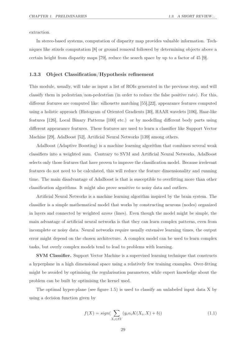
1.3.3 Object Classification/Hypothesis refinement
This module, usually, will take as input a list of ROIs generated in the previous step, and will
classify them in pedestrian/non-pedestrian (in order to reduce the false positive rate). For this,
different features are computed like: silhouette matching [55],[22], appearance features computed
using a holistic approach (Histogram of Oriented Gradients [30], HAAR wavelets [106], Haar-like
features [126], Local Binary Patterns [100] etc.) or by modelling different body parts using
different appearance features. These features are used to learn a classifier like Support Vector
Machine [29], AdaBoost [52], Artificial Neural Networks [139] among others.
AdaBoost (Adaptive Boosting) is a machine learning algorithm that combines several weak
classifiers into a weighted sum. Contrary to SVM and Artificial Neural Networks, AdaBoost
selects only those features that have proven to improve the classification model. Because irrelevant
features do not need to be calculated, this will reduce the feature dimensionality and running
time. The main disadvantage of AdaBoost is that is susceptible to overfitting more than other
classification algorithms. It might also prove sensitive to noisy data and outliers.
Artificial Neural Networks is a machine learning algorithm inspired by the brain system. The
classifier is a simple mathematical model that works by constructing neurons (nodes) organized
in layers and connected by weighted axons (lines). Even though the model might be simple, the
main advantage of artificial neural networks is that they can learn complex patterns, even from
incomplete or noisy data. Neural networks require usually extensive learning times, the output
error might depend on the chosen architecture. A complex model can be used to learn complex
tasks, but overly complex models tend to lead to problems with learning.
SVM Classifier. Support Vector Machine is a supervised learning technique that constructs
a hyperplane in a high dimensional space using a relatively few training examples. Over-fitting
might be avoided by optimising the regularisation parameters, while expert knowledge about the
problem can be built by optimising the kernel used.
The optimal hyper-plane (see figure 1.5) is used to classify an unlabeled input data X by
using a decision function given by
f(X) = sign(∑
Xi∈SV
(yiαiK(Xi, X) + b)) (1.1)
29

1.4. FEATURES CHAPTER 1. PRELIMINARIES
!"
!#
Figure 1.5: For a SVM trained on two-class problem, it is shown the maximum-margin hyperplane(along with the margins)
where SV is the set of support vector items Xi, b is the offset value, K is the kernel function and
αi are the optimized Lagrange parameters.
In this thesis, we have chosen to work only with Support Vector Machine classifier, due to fast
training and testing time. There exist different types of kernel functions that could be used with
the SVM. Among them, we have chosen to perform experiments with the Linear kernel for a fast
classification step.
In the next section we are going to present some of the significant features that are going to
be used across this thesis.
Figure 1.6: A pyramid as seen from two points of view
1.4 Features
Features, in the context of computer vision, represent different attributes or aspects of a particular
image. For example, in figure 1.6 is presented how a pyramid is seen from two different points
of view. In the same way, different features will ideally reveal various information about the image.
30

CHAPTER 1. PRELIMINARIES 1.4. FEATURES
In recent years, a large amount of features were developed. In what follows, we are going to
present a few features that are either widely used, or represent a reference point in literature,
and will be further used in various chapters of the thesis.
1.4.1 Histogram of Oriented Gradients (HOG)
Gradient based features have become very popular due to the robust results obtained in both
the sparse version (Scale Invariant Feature Transformation - SIFT [89]) and dense representation
(Histogram of Oriented Gradients - HOG [30]). HOG represents, currently, a state of the art
feature for pedestrian classification.
Local object appearance can be well characterised by the distribution of local intensity gradients
or edge directions. In the case of HOG, this is performed dividing the image into small cells. For
each cell a 1-D histogram is constructed containing the gradient orientations. By normalising
the obtained histogram inside bigger regions called blocks, it is obtained a better invariance to
illumination conditions. The final feature vector is constructed by the simple concatenation of
the computed histograms. In figure 1.7 are presented the main steps for computation of HOG
features.
1.4.2 Local Binary Patterns (LBP)
In comparison with HOG, that is used to capture edge or local shape information[100], local
binary pattern (LBP) operator is a texture descriptor that is widely used due to its invariance to
gray level changes.
There exist different methods to compute LBP, varying by different choice of parameters. In
order to compute the LBP operator we use the method described by Wang et al. [131], because
has proven to be one of the most robust. In a formal manner the operator can be described by
equation 1.2.
LBPp,r(c) =∑
i∈Np,r(c)
s(Ii − Ic) ∗ 2p (1.2)
where p is the number of pixels in a considered neighbourhood, r is the radius of the neighbourhood,
c are the coordinates of the central pixel, Np,r(c) represents the set of coordinates for the pixels
found at radius r from the central pixel, and s(x) is defined by equation 1.3.
31

1.4. FEATURES CHAPTER 1. PRELIMINARIES
!"#$%&'()*+%$$%*
**************,*
***********-"&".#
/"$0.1)*+#%2')314
5)'+61)2*7"1)*
'31"*40%1'%&*%32*
"#')31%1'"3*-)&&*
*!"#$%&'(%1'"3*"8*
"7)#&%00'3+*9&"-:4*
**/"&&)-1*;<=4*"7)#
16)*2)1)-1'"3*>'32">*
?30.1*?$%+)
Figure 1.7: HOG Feature computation
32

CHAPTER 1. PRELIMINARIES 1.4. FEATURES
s(x) =
1, if x ≥ 0
0, otherwise(1.3)
�������� ��������� �������
Figure 1.8: Examples of neighbourhood used to calculate a local binary pattern, where p are thenumber of pixels in the neighbourhood, and r is the neighbourhood radius
The main steps to compute LBP are:
• Like in the case of HOG, the ROI is divided into cells of 8× 8 pixels.
• Each pixel in a given cell is compared with the pixels in a considered neighbourhood and
a bit-string is constructed. This vicinity region is usually considered a circle as shown in
figure 1.8.
• The bit-string has the same length as the number of pixels in the neighbourhood, and is
constructing by comparing the value of a pixel with the pixels in the vicinity. If the center
pixel’s value is smaller than the neighbour’s value , then in the bit-string a ”1” will be
written, otherwise a ”0”, like showed in figure 1.9. Because in this approach a large number
of patterns can be created that could introduce noise in the classification process, only the
uniform patterns are considered. A uniform pattern, as seen in figure 1.10, is defined by
those pattern that lead to a maximum of two 0-1 transitions.
• In the following step, over each cell, a histogram is computed based on the decimal valued
of transformed bit-string.
• The histograms of all cells are concatenated and normalised. This gives the final feature
vector for the considered window.
1.4.3 Local Gradient Patterns (LGP)
LBP features are sensitive to local intensity variations and therefore could lead to many different
patterns in a small region. This might affect the performance of some classifiers. To overcome
33

1.4. FEATURES CHAPTER 1. PRELIMINARIES
�� �� ��
�� �� ��
��� �� ��
�� �� ��
��
���
��
��� �� ��
� � �
� �
� � �
�� �����
��������
�� ���������������
Figure 1.9: Local binary pattern computation for a given pixel. In this example the pixel forwhich the computation is performed is the central pixel having the intensity value 88.
������������� ��������������
����������������� ��������������
Figure 1.10: Examples of Uniform (a) and non-uniform patterns (b) corresponding for LBPcomputed with r = 1 and p = 8. There exist a total of 58 uniform local binarry pattern plusone(for others)
this, Jun et al. [72] proposed a novel representation called Local Gradient Patterns (LGP).
LBPp,r(c) =∑
i∈Np,r(c)
s(Gi −G) ∗ 2p (1.4)
where gradient s is defined in equation 1.3, Gp is defined in 1.5 as the absolute difference
between the central pixels intensity Ic and its neighbouring pixel Ii, and G is defined in equation
1.6
Gi = |Ii − Ic| (1.5)
G =1
p
p−1∑
n=0
Gn (1.6)
This operator is computed in a similar manner as LBP. Instead of working on intensity values
of the pixels, it employs gradient values of the neighbourhood pixels (see equation 1.4). The
gradient is computed as the absolute value of intensity difference between the given pixel and its
neighbouring pixels. The central pixel value is replaced by the average of gradient values (see
figure 1.11).
34

CHAPTER 1. PRELIMINARIES 1.4. FEATURES
�� �� ��
�� �� ��
��� �� ��
� � �
��
�� �
� � �
� �
� � �
�� ���� ��������
�����������������
�������
���� ��
Figure 1.11: Local gradient pattern operator computed for the central pixel having the intensity88.
1.4.4 Color Self Similarity (CSS)
Recent work has shown that local low-level features are particularly efficient ([34], [132]). In
[127] a new feature (CSS ), is proposed for images in the visible spectrum, based on second order
statistics of colors. This method takes advantage of locally similar colors within an analysis
window.
This window is first divided into blocks of 8× 8 pixels. For a given color space, like RGB and
HSV, a histogram with 3× 3× 3 bins is computed for each block. Every block is then compared
to all others blocks using histogram intersection resulting in a vector of similarities. Finally, a
L2-normalization is applied to that similarity vector.
1.4.5 Haar wavelets
Haar wavelets were introduced by Papageorgiou and Poggio [106]. The idea behind this type of
features is to compute the difference between the sum of intensities in two rectangular areas in
different configurations and sizes (see figure 1.12.a),1.12.b), 1.12.c)). These were extended by
Viola et al. [126]. They introduced two new configurations for the rectangular areas (see figure
1.12.d), 1.12.e)) and also proposed a classifier based on layers of weak classifiers (AdaBoost).
1.4.6 Disparity feature statistics (Mean Scaled Value Disparity)
A feature that is interesting from the perspective of using disparity map, is the disparity feature
statistics proposed by Walk et al. [128].
The main idea behind these features is that even if the heights of pedestrians are not identical,
they are still very similar. The disparity statistics proposed in [128] are based on the invariant
property of disparity map, that the ratio of disparity and observed heigh is inversely proportional
to the 3D object height.
In order to make the disparity statistics features independent of the distance to the object, in
a scenario of sliding window search, the disparity values are divided by the appropriate scale level
35
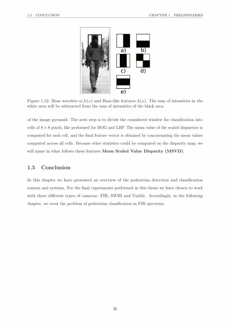
1.5. CONCLUSION CHAPTER 1. PRELIMINARIES
Figure 1.12: Haar wavelets a),b),c) and Haar-like features d),e). The sum of intensities in thewhite area will be subtracted from the sum of intensities of the black area.
of the image pyramid. The next step is to divide the considered window for classification into
cells of 8× 8 pixels, like performed for HOG and LBP. The mean value of the scaled disparities is
computed for each cell, and the final feature vector is obtained by concatenating the mean values
computed across all cells. Because other statistics could be computed on the disparity map, we
will name in what follows these features Mean Scaled Value Disparity (MSVD).
1.5 Conclusion
In this chapter we have presented an overview of the pedestrian detection and classification
sensors and systems. For the final experiments performed in this thesis we have chosen to work
with three different types of cameras: FIR, SWIR and Visible. Accordingly, in the following
chapter, we treat the problem of pedestrian classification in FIR spectrum.
36
When you can’t make them see the light,
make them feel the heat.
Ronald Reagan
2Pedestrian detection and classification in Far Infrared Spectrum
Contents
2.1 Related Work . . . . . . . . . . . . . . . . . . . . . . . . . . . . . . . . . 40
2.2 Datasets . . . . . . . . . . . . . . . . . . . . . . . . . . . . . . . . . . . . 42
2.2.1 Dataset ParmaTetravision . . . . . . . . . . . . . . . . . . . . . . . . . . 43
2.2.2 Dataset RIFIR . . . . . . . . . . . . . . . . . . . . . . . . . . . . . . . . 46
2.3 A new feature for pedestrian classification in infrared images: In-
tensity Self Similarity . . . . . . . . . . . . . . . . . . . . . . . . . . . . 49
2.4 A study on Visible and FIR . . . . . . . . . . . . . . . . . . . . . . . . 52
2.4.1 Preliminaries . . . . . . . . . . . . . . . . . . . . . . . . . . . . . . . . . 53
2.4.2 Feature performance comparison on FIR images . . . . . . . . . . . . . 53
2.4.3 Feature performance comparison on Visible images . . . . . . . . . . . . 55
2.4.4 Visible vs FIR . . . . . . . . . . . . . . . . . . . . . . . . . . . . . . . . 55
2.4.5 Visible & FIR Fusion . . . . . . . . . . . . . . . . . . . . . . . . . . . . 56
2.5 Conclusions . . . . . . . . . . . . . . . . . . . . . . . . . . . . . . . . . . 56
In this chapter, we study the pertinence of using a monocular FIR camera for the task of
pedestrian detection and classification. In recent years, the cost of infrared (IR) cameras has
decreased, making them an interesting alternative to visible cameras for pedestrian detection
systems ([10], [134], [115], [86]). Moreover, infrared cameras still provide pertinent and discrimi-
native information even in difficult illumination conditions (i.e. night, fog) and they are less prone
to confusion caused by colors, textures and shadows belonging to objects other than pedestrians.
Although there exists different IR sensors characterized by their wavelength, FIR camera seems
to be the most suitable for distinguishing hot targets like pedestrians. This ability represents an
advantage of FIR cameras over visible ones, especially during the night. Despite this, pedestrian
detection in IR images remains a challenging task, because the system has to deal not only
37

2.1. RELATED WORK CHAPTER 2. PEDESTRIAN.. FIR SPECTRUM
with the problem of their variability in posture, range, orientation, but also with the lack of
texture information. Therefore, texture can be an advantage, due to less distractions in the
image, and disadvantage, due to less information available. Another challenge is that objects
other than pedestrian, like vehicles, animals, electricity sources, appear also as hot targets in the
FIR spectrum.
2.1 Related Work
Usually, the sliding window technique, mostly used in the Visible domain, is not suitable for
real-time object detection application that uses a complex classifier. In response to this, Infrared
domain offers the possibility of generating a smaller number of hypothesis to be tested, therefore
becoming an interesting alternative to the Visible spectrum. Moreover, thermal Infrared has
a clear advantage over Visible spectrum during the night, where it can still provide relevant
information about the environment.
For Region of Interest (ROI) generation in FIR images a natural solution would be to use a
threshold, like in [115], or even better an adaptive threshold by assuming that non-pedestrian
intensities follow a Gaussian distribution [13]. Unfortunately, the problem of estimating an
appropriate threshold remains a key issue because the pedestrian intensities vary with respect to
range and outside temperature.
Erturk [42] presents a region of interest extraction in infrared images based on one-bit transform.
Potential interest regions are obtained by using a target mask, followed by a comparison of the
original image histogram with the masked image histogram in order to obtain an automated
threshold value. This method was tested only on static images and is not followed by a classification
step.
Kim and Lee [73] present a region of interest generation method specialized for nighttime
pedestrian detection using far-infrared (FIR) images. They respond to the problem of finding
a good intensity threshold, by working with image segments and also using the low-frequency
characteristics of the FIR images.
Wang et al. [129] try to improve the local contrast between targets and background in the
static infrared images, by proposing a background model. In the same time to filter the false
negatives a ramp loss function is used to learn the characteristics of a pedestrian. Liu et al. [88]
use a pixel-gradient oriented vertical projection approach in order to estimate the vertical image
stripes that might contain pedestrians. Afterwards, a local thresholding image segmentation is
adopted to generate ROIs more accurately within the estimated vertical stripes.
Other approaches consists in detecting warm symmetrical objects with specific size and aspect
38
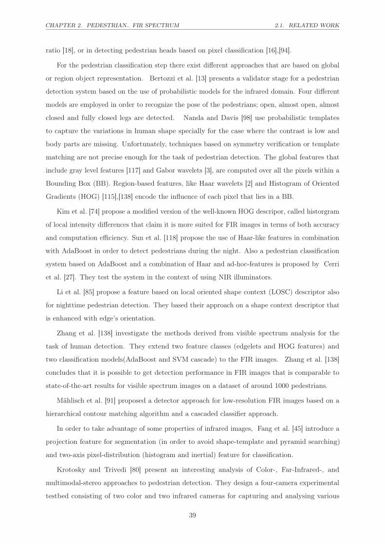
CHAPTER 2. PEDESTRIAN.. FIR SPECTRUM 2.1. RELATED WORK
ratio [18], or in detecting pedestrian heads based on pixel classification [16],[94].
For the pedestrian classification step there exist different approaches that are based on global
or region object representation. Bertozzi et al. [13] presents a validator stage for a pedestrian
detection system based on the use of probabilistic models for the infrared domain. Four different
models are employed in order to recognize the pose of the pedestrians; open, almost open, almost
closed and fully closed legs are detected. Nanda and Davis [98] use probabilistic templates
to capture the variations in human shape specially for the case where the contrast is low and
body parts are missing. Unfortunately, techniques based on symmetry verification or template
matching are not precise enough for the task of pedestrian detection. The global features that
include gray level features [117] and Gabor wavelets [3], are computed over all the pixels within a
Bounding Box (BB). Region-based features, like Haar wavelets [2] and Histogram of Oriented
Gradients (HOG) [115],[138] encode the influence of each pixel that lies in a BB.
Kim et al. [74] propose a modified version of the well-known HOG descripor, called historgram
of local intensity differences that claim it is more suited for FIR images in terms of both accuracy
and computation efficiency. Sun et al. [118] propose the use of Haar-like features in combination
with AdaBoost in order to detect pedestrians during the night. Also a pedestrian classification
system based on AdaBoost and a combination of Haar and ad-hoc-features is proposed by Cerri
et al. [27]. They test the system in the context of using NIR illuminators.
Li et al. [85] propose a feature based on local oriented shape context (LOSC) descriptor also
for nighttime pedestrian detection. They based their approach on a shape context descriptor that
is enhanced with edge’s orientation.
Zhang et al. [138] investigate the methods derived from visible spectrum analysis for the
task of human detection. They extend two feature classes (edgelets and HOG features) and
two classification models(AdaBoost and SVM cascade) to the FIR images. Zhang et al. [138]
concludes that it is possible to get detection performance in FIR images that is comparable to
state-of-the-art results for visible spectrum images on a dataset of around 1000 pedestrians.
Mählisch et al. [91] proposed a detector approach for low-resolution FIR images based on a
hierarchical contour matching algorithm and a cascaded classifier approach.
In order to take advantage of some properties of infrared images, Fang et al. [45] introduce a
projection feature for segmentation (in order to avoid shape-template and pyramid searching)
and two-axis pixel-distribution (histogram and inertial) feature for classification.
Krotosky and Trivedi [80] present an interesting analysis of Color-, Far-Infrared-, and
multimodal-stereo approaches to pedestrian detection. They design a four-camera experimental
testbed consisting of two color and two infrared cameras for capturing and analysing various
39

2.2. DATASETS CHAPTER 2. PEDESTRIAN.. FIR SPECTRUM
configuration permutations for pedestrian detection, thus providing an in-depth analysis for the
use of color and FIR. Their conclusion is that on the tested images, visible images provided better
results than the infrared ones.
Olmeda et al. [102] propose a pedestrian detection system based on discrete features in thermal
infrared images, these descriptors are matched with defined regions of the body of a pedestrian.
In case of a match it creates a regions of interest which is then classified using an SVM. Olmeda
et al. [103] present a study on pedestrian classification and detection in FIR images using a
descriptor named Histograms of Oriented Phase Energy combined with a latent variable SVM
approach.
With the exception of the dataset used by Olmeda et al. [103], from our knowledge, the other
articles do not make public the acquired images. As a consequence, it is quite difficult to compare
the proposed approaches.
2.2 Datasets
Although there exists a reasonable number of benchmark datasets for the pedestrian detection in
the Visible domain1, in case of FIR images most of the datasets are not publicly available.
Datasets like that proposed by Simon Lynen [113], Davis and Keck [32], Davis and Sharma [33]
focus mostly on surveillance application, therefore they use a fixed-camera setup.
Recently Olmeda et al. (2013) [103] proposed a dataset2 acquired with an Indigo Omega,
having and image resolution of 164× 129. The dataset is divided in two parts: one that tacks
the problem of pedestrian classification (OlmedaFIR-Classification), and the other one that is
constructed for the problem of pedestrian detection (OlmedaFIR-Detection). In figure 2.1 are
presented examples of images from the OlmedaFIR-Detection dataset. Unfortunately, it does
not contain also information from the Visible spectrum, therefore making difficult a complete
assessment of the FIR performance.
An interesting dataset that contains both FIR and Visible images is proposed by Bertozzi
et al. [12]. Unfortunately, the dataset had just a small number of annotations (around 1000 BB),
therefore it might not provide statistically relevant results. Moreover, this dataset is not publicly
available3.
1The Visible domain dataset will be treated in chapter 52We will further refer to this dataset as OlmedaFIR3This dataset is maintained by Vislab. Terms and conditions for usage may apply. http://vislab.it/
40

CHAPTER 2. PEDESTRIAN.. FIR SPECTRUM 2.2. DATASETS
a) b)
Figure 2.1: Images examples from Oldemera dataset a),b)
In order to respond to the deficiencies of the datasets proposed by Olmeda et al. [103]
and Bertozzi et al. [12], on one hand, we propose a new benchmark for pedestrian detection
and classification in FIR images, which consists of sequences acquired in an urban environment
with two cameras (FIR and color) mounted on the exterior of a vehicle. We will further refer
to the proposed dataset as RIFIR4. On the other hand, we have extended the annotations on
the dataset proposed by Bertozzi et al. [12]. We will further refer to the extended dataset as
ParmaTetravision.
In table 2.1 we present an overview of existing pedestrian datasets. In what follows we will
present dataset statistics for the both ParmaTetravision and RIFIR.
2.2.1 Dataset ParmaTetravision
Dataset ParmaTetravision contains information taken from two visible and two infrared cameras
and was provided to us by VisLAB laboratory in Parma Italy [12]. In a previous work [16], there
were annotated around 1000 pedestrians BB (table 2.2), but we felt that this will not provide a
large enough dataset in order to compare the performance of different features. Thus, we have
extended the annotation to include a much larger number of images and manually annotated BB
for both training and testing5.
Pedestrian Non-Pedestrian Overall
Number of BB (IR) 1089 1003 2092
Table 2.2: ParmaTetravision[Old] Dataset statistics
4The dataset is publicly available at the web address: www.vision.roboslang.org5For training we have use sequences 1 and 5 from the dataset; while for testing sequences 2 and 6.
41

2.2.DATASETSCHAPTER2.PEDESTRIAN..FIRSPECTRUM
Data
set
Properties
Train
ing
Test
ing
Acq
uis
itio
nse
tup
Envir
onm
ent
Infr
are
dV
isib
leO
cclu
sion
Label
Ste
reo
Res
olu
tion
No.
Img.
No.
Uniq
ue
Ped
No.
BB
No.
Img.
No.
Ped
.BB
No.
Img.
No.
Ped
.BB
ET
HZ
Ther
-m
alIn
frare
dD
ata
set[113]
Surv
eillance
Road
Sce
ne
FIR
NO
NO
No
324×
256
4318
22
6500
--
--
OSU
Ther
mal
Ped
estr
ian
Data
base
[32]
Surv
eillance
Road
Sce
ne
FIR
NO
NO
No
360×
240
284
-984
--
--
OSU
Colo
r-T
her
mal
Data
base
[33]
Surv
eillance
Road
Sce
ne
FIR
YE
SN
ON
o320×
240
17089
48
--
--
-
RG
B-N
IRSce
ne
Data
set[24]
Surv
eillance
Outd
oor
NIR
YE
S-
No
1024×
768
477
--
--
--
Olm
edaFIR
-C
lass
ifica
tion[1
03]
Mobile
Road
Sce
ne
FIR
NO
NO
NO
164×
129
81529
-∼
16000
∼10000
∼10000
∼6000
∼6000
Olm
edaFIR
-D
etec
tion[1
03]
Mobile
Road
Sce
ne
FIR
NO
NO
NO
164×
129
15224
-8400
∼6000
∼4300
∼5000
∼4100
Parm
a-
Tet
ravis
iona[1
2]
Mobile
Road
Sce
ne
FIR
YE
SY
ESb
YE
S320×
240
18578
280
∼18000
∼10000
∼9000
∼8000
∼8800
RIF
IR(P
ropose
dD
ata
set)
Mobile
Road
Sce
ne
FIR
YE
SY
ESb
NO
650×
480
∼24000
171
∼20000
∼15000
∼14000
∼9300
∼6200
Tab
le2.
1:D
atas
ets
com
pari
son
for
ped
estr
ian
clas
sific
atio
nan
dde
tect
ion
inFIR
imag
es
aD
ata
set
stati
stic
sbase
don
our
annota
tions
bO
nly
two-c
lass
occ
lusi
on
label
sav
ailable
:occ
luded
or
not
occ
luded
42

CHAPTER 2. PEDESTRIAN.. FIR SPECTRUM 2.2. DATASETS
As presented in table 2.3, the final dataset contains 10240 images for training having
annotated 11554 pedestrian BB in visible spectrum and 9386 BB in IR spectrum; and 8338 images
for testing with 9386 annotated pedestrian BB in visible and 8801 in IR. The disagreement in the
number of pedestrian from visible and IR is due to differences in camera optics and positioning.
For the final dataset used for the problem of pedestrian classification, we have retained only
those BB that have a height above 32px, are visible in both cameras and don’t present major
occlusions. Therefore in the end we have 6264 pedestrian BB for training and 5743 pedestrian
BB for testing. Furthermore, for the problem of pedestrian classification we have extracted
26316 negative BB for training and 14823 for testing.
Sequence Train Sequence Test Overall
Number of frames 10240 8338 18578
Number of unique pedestrians 120 160 280
Number of annotated pedestrian
BB (Visible)
11554 11451 23005
Number of annotated pedestrian
BB (IR)
9386 8801 18187
Number of pedestrian BB visible
in both cameras with height > 32 px,
and not presented major occlusions
6264 5743 12007
Number of negative BB annotated 26316 14823 41139
Table 2.3: ParmaTetravision Dataset statistics
In figure 2.3 is presented the height histogram for the annotated pedestrians for both Training
and Testing. Most of the pedestrians have a height inferior to 150 pixels. Due to a small difference
in optics, the pedestrians in FIR images will appear slightly larger than those in Visible images.
In the dataset, annotated pedestrians tend to be concentrated into the same regions. In figure
2.2 is presented a normalized heat map obtained by plotting the annotated pedestrian BBs. The
heat map is presented as in indicator that even if pedestrian tend to concentrate in the same
region, different optics and environment will produce various heat maps. In figure 2.4 is presented
an example of image from the ParmaTetravision dataset.
43

2.2. DATASETS CHAPTER 2. PEDESTRIAN.. FIR SPECTRUM
(a) (b)
Figure 2.2: Heat map of training for ParmaTetravision Dataset: a) Visible b) FIR
!
""""""#!!
""""""$!!!
""""""$#!!
""""""%!!!
""""""%#!!
""""""&!!!
""""""&#!!
""""""'!!!
""""""'#!!
%# #! (# $!! $%# $#! $(# %!! %%# %#! %(# &!!
)*+*,-./01"2*/34-"5)/6*7,8
9/,/:7*;<
=>?:*."@A"BB
!
""""""#!!
""""""$!!!
""""""$#!!
""""""%!!!
""""""%#!!
""""""&!!!
%# #! '# $!! $%# $#! $'# %!! %%# %#! %'# &!!
()*)+,-./0"1).23,+"4(.5)6+7
8.+.96)
:;<=>9)-"?@"AA
(a) (b)
Figure 2.3: Pedestrian height distribution of training (a) and testing (b) sets for ParmaTetravision
a) b)
Figure 2.4: Images examples from ParmaTetravision dataset a) Visible spectrum b) Far-infraredspectrum
44

CHAPTER 2. PEDESTRIAN.. FIR SPECTRUM 2.2. DATASETS
2.2.2 Dataset RIFIR
For the acquired dataset, we have used two cameras: one Visible domain camera (colour) with
a resolution of 720 × 480 and a FIR camera with a resolution of 640 × 480. In table 2.4 are
presented some information regarding the employed FIR camera6.
Characteristic Value
Pixel Resolution 640× 480
Focal length 24.5 mm
Spectral range 7.5µm to 13µm
Object temperature range −20 to +150◦C
Accuracy ±2% of reading
Image frequency 50Hz
Control GigE Vision and GenICam compatible
Power system 12/24 VDC, 24 W absolute max
Operating Environment Operation Temperature: −15◦C to
+50◦C; Humidity: 0− 95%
Table 2.4: Infrared Camera specification
Due to difference in camera optics and position, we had to annotate the pedestrian indepen-
dently in the Visible and FIR images. As presented in table 2.5 the final dataset contains 15023
images in training with 19190 annotated pedestrian BBs in Visible spectrum and 14356 in FIR
spectrum; and 9373 images for testing with 7133 annotated pedestrian BBs in Visible and 6268
in the FIR domain.
Following the same methodology as in the case of ParmaTetravision dataset, for the final
constructed classification dataset we have only considered those pedestrians with a height above
32 pixels, that are visible in both cameras, and do not present occlusions. In consequence, there
are 9202 pedestrian BB for training and 2034 for testing. In what concerns the negative BBs, we
have considered 25608 in training set and 24444 in testing.
6The camera was provided by Laboratoire d’Electronique, d’Informatique et de l’Image (Le2i) http://le2i.
cnrs.fr/
45

2.2. DATASETS CHAPTER 2. PEDESTRIAN.. FIR SPECTRUM
In figure 2.5 is presented the height histogram for the annotated pedestrian in both Training
and Testing. While in the ParmaTetravision dataset most of the pedestrians had a height below
150 pixels, in the case of RIFIR dataset, most of the pedestrians have a height below 100 pixels,
thus making the dataset more challenging. In figure 2.6 is presented the heat map, for both
Visible and FIR, obtained by superimposing the annotated pedestrians. Small differences are due
to camera optics and positioning. In figure 2.7 is presented an extract from the RIFIR dataset.
Sequence Train Sequence Test Overall
Number of frames 15023 9373 24396
Number of unique pedestrians 138 33 171
Number of annotated pedestrian
BB (Visible)
19190 7133 26323
Number of annotated pedestrian
BB (IR)
14356 6268 20624
Number of pedestrian BB visible
in both cameras with height > 32 px
9202 2034 11236
Number of negative BB annotated 25608 24444 50052
Table 2.5: RIFIR Dataset statistics
!
"!!!
#!!!
$!!!
%!!!
&!!!
'!!!
(!!!
)*+*,-.
/0
#& &! (& "!! "#& "&! "(&#!! ##& #&! #(&$!! $#& $&! $(& %!! %#&
1.2.+34*56 7.*893 :1*;.-+<
=>?,.4@ABB
!
""""""#!!
""""""$!!!
""""""$#!!
""""""%!!!
""""""%#!!
""""""&'(')*+
"""""",-
%# #! .# $!! $%# $#! $.#%!! %%# %#! %.#/!! /%# /#! /.# 0!! 0%#
1+2+(34'56 7+'893 :1';+*(<
=>?)+4@ABB
(a) (b)
Figure 2.5: Pedestrian height distribution of training (a) and testing sets (b) for RIFIR
46

CHAPTER 2. PEDESTRIAN.. FIR SPECTRUM 2.3. ISS
(a) (b)
Figure 2.6: Heat map of training for RIFIR Dataset: a) Visible, b) FIR
a) b)
Figure 2.7: Images examples from RIFIR dataset a) Visible spectrum b) Far-infrared spectrum
2.3 A new feature for pedestrian classification in infrared images:
Intensity Self Similarity
Motivation In [15], detection of pedestrians ROIs based on an algorithm of head detection
was combined with a classifier based on local and global SURF-based features. The local
features describe the appearance of an obstacle and are extracted from a codebook of scale and
rotation-invariant SURF descriptors. Whereas, global features, extracted from a set of interest
points, provide complementary information by characterizing the shape and the texture. The
disadvantage of SURF points used in the phase of ROI classification is that detected key points
repeat more often on background and less on the people even when looking at two consecutive
frames of a video [84]. Therefore, another type of descriptor is needed that will be more robust
to consecutive frames, like HOG or CSS.
47

2.3. ISS CHAPTER 2. PEDESTRIAN.. FIR SPECTRUM
Feature description Inspired by CSS, we propose an original feature representation, called
Intensity Self Similarity, adapted for FIR images. In contrast with images acquired with cameras
in visible spectrum, that can provide color information, those taken using FIR sensor, provide
only information about the pixel intensities, making CSS representation not suitable. After a
careful analysis of road scenes in FIR spectrum, we believe that FIR images emphasise several
intensity structures, since pixels within a pedestrian head region have approximately the same
intensity values, the arms intensity values seem to be similar and this also could be applied to
the leg areas. According to this, we propose a self similarity feature based on intensities values of
thermal images, rather than on color information.
Figure 2.8: Visualisation of Intensity Self Similarity using histogram difference computed atpositions marked with blue in the IR images. A brighter cell shows a higher degree of similarity.
We divide each pedestrian full-body BB into n blocks of 8× 8 pixels (see figure 2.8). After
computing a histogram for each block, we construct a similarity vector of n ∗ (n− 1)/2 elements,
by comparing the histogram of each block with the histograms of all the other blocks within a
given BB.
For the comparison of two histograms H1 and H2, we have tested different techniques like:
• Histogram Intersection:∑
i=1,histSizemin(H1[i], H2[i])
• Histogram Difference:∑
i=1,histSize |H1[i]−H2[i]|
• Chi Square Distance:∑
i=1,histSize(H1[i]−H2[i])2/H2[i]
48

CHAPTER 2. PEDESTRIAN.. FIR SPECTRUM 2.3. ISS
0 0.05 0.1 0.15 0.2 0.250.75
0.8
0.85
0.9
0.95
1
False Positive Rate
Cla
ssific
atio
n R
ate
Histogram IntersectionHistogram DifferenceChi−square distanceEmpirical Distribution
Figure 2.9: Performance of ISS feature on the dataset ParmaTetravision[Old] using differenthistogram comparison strategies
• Empirical Distribution:∑
i=1,histSize 1H1[i]≤H2[i]
Feature parameters optimisation This feature is used to feed up a fast, but efficient linear-
kernel SVM classifier. In order to validate the proposed feature we have used the dataset
ParmaTetravision[Old] that contains 1089 pedestrians. The pedestrian detection performances
are estimated by the precision rate, the recall rate and the F-measure, using a 10-fold Cross
Validation (CV) technique.
In figure 2.9 is plotted the ROC7 curve for each tested technique of histogram comparison.
Subsequently, we have chosen to use histogram difference rather than histogram intersection, like
[127], because it provided lower false positive rate for a high recall.
For the choice of block and histogram size, we have tested blocks of 8× 8 and 16× 16 pixels,
and six different histograms sizes. The results in terms of F-measure are presented in figure 2.10.
As it can be observed, the histogram size does not have a significant impact for the performance,
results varying just between ±0.5%. On the contrary, the block size, has a greater influence over
the results.
For the final configuration of ISS feature, we have chosen to use block size of 8 × 8 pixels,
histogram of 16 bins and histogram difference for comparison algorithm.
7Receiver operating characteristic
49
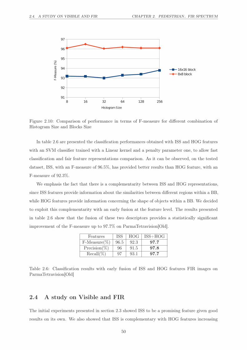
2.4. A STUDY ON VISIBLE AND FIR CHAPTER 2. PEDESTRIAN.. FIR SPECTRUM
! """"""#$ """"""%& """"""$' """"""#&! """"""&($
"""""")#
"""""")&
"""""")%
"""""")'
"""""")(
"""""")$
"""""")*
""""""#$+#$ ,-./0
""""""!+!,-./0
""""""1234.567892:;
<=>;73?6;@AB
Figure 2.10: Comparison of performance in terms of F-measure for different combination ofHistogram Size and Blocks Size
In table 2.6 are presented the classification performances obtained with ISS and HOG features
with an SVM classifier trained with a Linear kernel and a penalty parameter one, to allow fast
classification and fair feature representations comparison. As it can be observed, on the tested
dataset, ISS, with an F-measure of 96.5%, has provided better results than HOG feature, with an
F-measure of 92.3%.
We emphasis the fact that there is a complementarity between ISS and HOG representations,
since ISS features provide information about the similarities between different regions within a BB,
while HOG features provide information concerning the shape of objects within a BB. We decided
to exploit this complementarity with an early fusion at the feature level. The results presented
in table 2.6 show that the fusion of these two descriptors provides a statistically significant
improvement of the F-measure up to 97.7% on ParmaTetravision[Old].
Features ISS HOG ISS+HOGF-Measure(%) 96.5 92.3 97.7
Precision(%) 96 91.5 97.8
Recall(%) 97 93.1 97.7
Table 2.6: Classification results with early fusion of ISS and HOG features FIR images onParmaTetravision[Old]
2.4 A study on Visible and FIR
The initial experiments presented in section 2.3 showed ISS to be a promising feature given good
results on its own. We also showed that ISS is complementary with HOG features increasing
50

CHAPTER 2. PEDESTRIAN.. FIR SPECTRUM 2.4. A STUDY ON VISIBLE AND FIR
the F-Measure. Nevertheless, the testing dataset was fairly small. Consequently, we decided to
extend the experiments to include more features and several datasets.
In this section we are going to compare the performance of different features like HOG, LGP,
LBP and the proposed ISS on the Far Infrared domain, using three datasets: ParmaTetravision,
OlmedaFIR-Classification and the proposed RIFIR. Moreover, a comparison between the FIR
and Visible Domain is conducted using the datasets ParmaTetravision and RIFIR.
2.4.1 Preliminaries
For all three databases, in order to be consistent in the classification process, we have resized the
annotated BBs to a size of 48 pixels in width and 96 in height.
HOG features are computed on cells of 8×8 pixels, accumulated on overlapping 16× 16 pixel
blocks, with a spatial shift of 8 pixels. This results in a number of 1980 features.
LBPs and LGPs features are computed using cells 8×8 pixels, and a maximum number of
0− 1 transitions of 2. This results in a number of 4248 features.
ISS is computed on cells of 8×8 pixels, histogram size of 16 pixels and histogram difference.
This results in a number of 5944 features.
These features are fed to a linear SVM classifier. For this, we have used the library LIBLINEAR
[44].
All the results in this section are reported in term of ROC curve (false positive rate vs
classification rate), considering as reference point the false positive rate obtained for a classification
rate of 90%.
2.4.2 Feature performance comparison on FIR images
First of all, we decided to evaluate the performance of the considered features (HOG, LBP, LGP,
ISS) in the FIR domain. In figure 2.11 is presented the performance of using each individual
feature independently on dataset RIFIR (figure 2.11.a), ParmaTetravision (figure 2.11.b) and
Oldemera-Classification(figure 2.11.c).
On datasets RIFIR and Oldemera-Classification the best performing feature is LBP, followed
closely by LGP. On ParmaTetravision dataset, the best performing feature is LGP followed closely
by LBP. On datasets ParmaTetravision and Oldemera-Classification HOG features performs
better than ISS, while on RIFIR the situation is reversed.
In our opinion, the difference in performance between features comes from the fact that even if
all three datasets were obtain using FIR cameras, there is a difference in sensors, road scenes and
environmental conditions. It seems that as single feature, the Local Binary/Gradient Patterns
51

2.4. A STUDY ON VISIBLE AND FIR CHAPTER 2. PEDESTRIAN.. FIR SPECTRUM
0 0.05 0.1 0.15 0.2 0.250.75
0.8
0.85
0.9
0.95
1
False Positive Rate
Cla
ss
ific
ati
on
Ra
te
HOG (IR): 0.1561
LBP (IR) : 0.0019
LGP (IR) : 0.0107
ISS (IR) : 0.0319
(a)
0 0.02 0.04 0.06 0.08 0.1 0.12
0.88
0.9
0.92
0.94
0.96
0.98
1
False Positive Rate
Cla
ss
ific
ati
on
Ra
te
HOG (IR): 0.0225
LBP (IR) : 0.0067
LGP (IR) : 0.0042
ISS (IR) : 0.0236
(b)
0 0.01 0.02 0.03 0.04 0.05 0.06
0.94
0.95
0.96
0.97
0.98
0.99
1
False Positive Rate
Cla
ss
ific
ati
on
Ra
te
HOG (IR) 0.000317
LBP (IR) 0.0000001
LGP (IR) 0.000045
ISS (IR) 0.002449
(c)
10−4
10−2
100
10−3
10−2
10−1
100
False Positive Rate
Fa
lse
Ne
ga
tiv
e R
ate
(m
iss
)
HOG (IR) 0.125
LBP (IR) 0.06
LGP (IR) 0.07
ISS (IR) 0.335
(d)
Figure 2.11: Performance comparison for features HOG, LBP, LGP and ISS in the FIR spectrumon datasets a) RIFIR b) ParmaTetravision c) Oldemera-classification. The reference point isconsidered the obtained false positive rate for a classification rate of 90%. In figure d) are alsoshown the results for Oldemera-classification but this time as miss-rate vs false positive rate. Inthis case the reference point is the miss rate obtained for a false positive rate of 10−4
are more adapted for the task of pedestrian classification in FIR images. Nevertheless, because
the features are complementary, we will test a fusion of features in section 2.4.5.
In figure 2.11.d) is presented a comparison between the considered features on the Oldemera-
classification, in terms of False Positive Rate vs False Negative Rate (miss rate), on a log-log
scale. We chose to present the results in this manner because this is the preferred approach of
Olmeda et al. [103]. The reference point is considered the false negative rate obtained for a false
positive rate of 10−4. We report slightly different results than that of Olmeda et al. [103] for
HOG and LBP features. Thus, for HOG we obtain a miss rate of 0.125 ( in comparison with the
reported 0.21 [103], and for LBP we obtain a miss rate of 0.06 (in comparison with the reported
0.41 [103]). The difference in results may come from slightly different implementation for the
features and from the use of different libraries for SVM classifier.
52

CHAPTER 2. PEDESTRIAN.. FIR SPECTRUM 2.4. A STUDY ON VISIBLE AND FIR
0 0.1 0.2 0.3 0.4 0.50.5
0.6
0.7
0.8
0.9
1
False Positive Rate
Cla
ss
ific
ati
on
Ra
te
HOG (Vis): 0.3480
LBP (Vis) : 0.0583
LGP (Vis) : 0.3382
ISS (Vis) : 0.2262
(a)
0 0.05 0.1 0.15 0.2 0.250.75
0.8
0.85
0.9
0.95
1
False Positive Rate
Cla
ss
ific
ati
on
Ra
te
HOG (Vis): 0.0524
LBP (Vis) : 0.0234
LGP (Vis) : 0.0325
ISS (Vis) : 0.077
(b)
Figure 2.12: Peformance comparison for the features HOG, LBP, LGP and ISS in the Visibledomain on datasets a) RIFIR, b) ParmaTetravision
2.4.3 Feature performance comparison on Visible images
For the second scenario, we decided to evaluate the features (HOG, LBP, LGP and ISS) in the
Visible domain on the datasets RIFIR and ParmaTetravision. The results are reported in figure
2.12. LBP continues to be one of the most robust features obtaining a false positive rate of 0.05
on RIFIR dataset and 0.02 on ParmaTetravision. For the other considered features the results
are quite different.
As it can be observed from the example images from both datasets, RIFIR color images have
more noise than the grayscale images from ParmaTetravision. This has a direct impact over the
performance of features based on gradient: HOG and LGP. Thus, while ISS features manage to
be more robust in the context of noise (RIFIR), HOG and LGP perform better on higher quality
images (ParmaTetravision).
2.4.4 Visible vs FIR
Having the performance of different features on both Visible and FIR domains, we can now
compare the two spectrums. In figure 2.13 is presented a comparison between the same feature
computed on Visible and FIR for the two databases: RIFIR and ParmaTetravision. On both
datasets, the features computed on the FIR images have a better performance than those computed
on Visible. We withhold from drawing a definite conclusion that FIR cameras will always perform
better than Visible ones because it depends on the quality of cameras used and also optics. What
we can definitely say is that on the tested dataset the FIR spectrum gives better results.
The performance difference on the RIFIR dataset between Visible and FIR is quite large for
LGP and LBP with a factor of approximatively 30. HOG and ISS features computed on FIR
53

2.5. CONCLUSIONS CHAPTER 2. PEDESTRIAN.. FIR SPECTRUM
result in a smaller number of false positives than the equivalent on Visible, with a factor of two,
on both datasets.
2.4.5 Visible & FIR Fusion
In section 2.4.4 we have showed that on the two considered datasets, for the task of pedestrian
classification, features computed on FIR images performed better than the counterpart computed
on Visible.
By fusing both spectrums, as seen in figure 2.14.a) for RIFIR and 2.14.b) for ParmaTetravision,
the false positive rate for a classification rate of 90%, is further reduced.
HOG features computed on Visible and FIR improve by a factor of two the results, in
comparison with just computing on FIR domain, for RIFIR dataset, and by a factor of five for
ParmaTetravision. For RIFIR dataset, the same factor of approximately two is obtained for LBP,
LGP, and ISS features, while on the ParmaTetravision the factor will be usually equal of larger
than five.
Features computed from FIR and Visible are highly complementary, and the use of the
two spectrums will always lower the error rate. Unfortunately, the information fusion is not
straightforward because two different cameras are used, one for FIR and one for Visible domain,
therefore there will always be difference in point of views. A correlation method between the two
domains is necessary. A possible hardware solution is to construct a camera capable of capturing
information from both light spectrums.
2.5 Conclusions
In this chapter we have described a new feature, ISS, that we adapted for the thermal images
and performed extensive tests on different datasets. Moreover, we have proposed a new dataset,
RIFIR, publicly available, in order to benchmark different algorithms of pedestrian detection
and classification. This dataset contains both Visible and FIR images, along with correlated
pedestrian and non-pedestrian bounding boxes in the two spectrums.
Moreover, a comparison between features computed on Visible and FIR spectrum is performed.
On the two tested datasets, Far-Infrared domain provided more discriminative features. Also, the
fusion of the two domains will further decrease the false positive error rate.
As shown in the related work section of this chapter, FIR spectrum was already studied in
different aspects for the task of pedestrian classification and detection. In comparison, in the
next chapter we present an analysis performed on another infrared spectrum, less popular: the
Short Wave Infrared.
54

CHAPTER 2. PEDESTRIAN.. FIR SPECTRUM 2.5. CONCLUSIONS
0 0.1 0.2 0.3 0.4 0.50.5
0.6
0.7
0.8
0.9
1
False Positive Rate
Cla
ssif
icati
on
Rate
HOG (IR): 0.1561
HOG (Visible) : 0.348
(a)
0 0.1 0.2 0.3 0.4 0.50.5
0.6
0.7
0.8
0.9
1
False Positive Rate
Cla
ssif
icati
on
Rate
HOG (IR): 0.0225
HOG (Visible) : 0.0524
(b)
0 0.05 0.1 0.15 0.2 0.250.75
0.8
0.85
0.9
0.95
1
False Positive Rate
Cla
ssif
icati
on
Rate
LBP (IR): 0.0019
LBP (Visible) : 0.0583
(c)
0 0.05 0.1 0.15 0.2 0.250.75
0.8
0.85
0.9
0.95
1
False Positive Rate
Cla
ssif
icati
on
Rate
LBP (IR): 0.0067
LBP (Visible) : 0.0234
(d)
0 0.1 0.2 0.3 0.4 0.50.5
0.6
0.7
0.8
0.9
1
False Positive Rate
Cla
ssif
icati
on
Rate
LGP (IR): 0.0107
LGP (Visible) : 0.3382
(e)
0 0.05 0.1 0.15 0.2 0.250.75
0.8
0.85
0.9
0.95
1
False Positive Rate
Cla
ssif
icati
on
Rate
LGP (IR): 0.0042
LGP (Visible) : 0.0325
(f)
0 0.05 0.1 0.15 0.2 0.250.75
0.8
0.85
0.9
0.95
1
False Positive Rate
Cla
ssif
icati
on
Rate
ISS (IR): 0.0319
ISS (Visible) : 0.2262
(g)
0 0.05 0.1 0.15 0.2 0.250.75
0.8
0.85
0.9
0.95
1
False Positive Rate
Cla
ssif
icati
on
Rate
ISS (IR): 0.0236
ISS (Visible) : 0.077
(h)
Figure 2.13: Performance comparison of features between Visible and FIR domains on: a), c), e),g) RIFIR dataset; b), d), f), h) ParmaTetravision dataset
55

2.5. CONCLUSIONS CHAPTER 2. PEDESTRIAN.. FIR SPECTRUM
0 0.05 0.1 0.15 0.2 0.250.75
0.8
0.85
0.9
0.95
1
False Positive Rate
Cla
ss
ific
ati
on
Ra
te
HOG (Vis) + HOG (IR): 0.0772
LBP (Vis) + LBP (IR): 0.0010
LGP (Vis) + LGP (IR): 0.0094
ISS (Vis) + ISS (IR): 0.0140
(a)
0 0.02 0.04 0.06 0.08 0.1 0.12
0.88
0.9
0.92
0.94
0.96
0.98
1
False Positive Rate
Cla
ss
ific
ati
on
Ra
te
HOG (Vis) + HOG (IR): 0.0042
LBP (Vis) + LBP (IR) : 0.00054
LGP (Vis) + LGP (IR) : 0.00067
ISS (Vis) + ISS (IR) : 0.0079
(b)
Figure 2.14: Individual feature fusion between Visible and FIR domain on a) RIFIR dataset b)ParmaTetravison dataset
56

There are two kinds of light - the glow that
illumines and the glare that obscures
James Thurber
3Pedestrian Detection and Classification in SWIR
Contents
3.1 Related work . . . . . . . . . . . . . . . . . . . . . . . . . . . . . . . . . 60
3.2 SWIR Image Analysis . . . . . . . . . . . . . . . . . . . . . . . . . . . . 60
3.3 Preliminary SWIR images evaluation for pedestrian detection . . . 62
3.3.1 Hardware equipment . . . . . . . . . . . . . . . . . . . . . . . . . . . . . 62
3.3.2 Dataset overview . . . . . . . . . . . . . . . . . . . . . . . . . . . . . . . 64
3.3.3 Experiments . . . . . . . . . . . . . . . . . . . . . . . . . . . . . . . . . 65
3.4 SWIR vs Visible . . . . . . . . . . . . . . . . . . . . . . . . . . . . . . . 69
3.4.1 Hardware equipment . . . . . . . . . . . . . . . . . . . . . . . . . . . . . 70
3.4.2 Dataset overview . . . . . . . . . . . . . . . . . . . . . . . . . . . . . . . 71
3.4.3 Experiments . . . . . . . . . . . . . . . . . . . . . . . . . . . . . . . . . 74
3.4.4 Discussion . . . . . . . . . . . . . . . . . . . . . . . . . . . . . . . . . . . 75
3.5 Conclusions . . . . . . . . . . . . . . . . . . . . . . . . . . . . . . . . . . 79
The purpose of this chapter is to investigate the suitability of the SWIR spectrum for the
problem of pedestrian detection and classification. In what follows we present related work
along with a short analysis of imagining in SWIR spectrum. Afterwards, in order to study the
performance of pedestrian detection and classification using SWIR cameras we have performed
two different experiments.
For the first one we have used a dataset provided by Vislab1 acquired with a low cost SWIR
camera. After having annotated three different sequences of images, we then evaluated if features
learned on visible images are suitable to be used on SWIR images. Other tests performed include
an SVM classifier based on deformable part models ([47], [48]), on grammar models [59] and a
HAAR based classifier [87].
1Artificial Vision and Intelligent Systems Laboratory (VisLab) of Parma University (Italy) - www.vislab.it
57

3.1. RELATED WORK CHAPTER 3. PEDESTRIAN... SWIR
Due to the limitations of the first dataset, for the second experiment we have acquired and
annotated a new set of images using two cameras, a SWIR and a Visible one. Thus, we are able
to compare pedestrian classification performances in the two wavelengths on a fairly large dataset.
For this, we compare several spatial features like HOG, LBP and LGP. Moreover, we propose to
enrich the intensity-based features from visible domain with features extracted from SWIR.
3.1 Related work
SWIR imaging began to be taken into consideration for computer vision applications because
it could bring useful contrast or complementary information to situations and applications
where visible or thermal imaging cameras are ineffective. This makes SWIR frequently used for
diverse applications such as aligning telecommunications fibers and sources, engineering optical
wave-guides, inspecting pharmaceutical quality, sorting recycled plastics, monitoring incoming
sources of raw agricultural products to groom out contamination by dirt, stones or packaging
debris, as well as grade sorting by moisture level or fat content, remote sensing of arid and
semiarid ecosystems[4], vegetation mapping in semiarid aread [37], ocean data color processing
[130]. Applications that mainly benefit from reduced scattering effects of longer wavelengths,
illumination from invisible sources (for example infrared active illumination or simply the night
glow from the upper atmosphere) or thermal emitting objects with temperatures above 150 C◦
are candidates for SWIR cameras [63].
Unlike Mid Wave IR (MWIR) and Long Wave IR (LWIR), SWIR cameras can image through
the windshield and thus be mounted in the vehicle’s cabin for a “driver’s eye” view of the way
ahead. Moreover, SWIR imagers have the ability to see clearer at long distance through the
atmosphere, making SWIR suitable for investigations in the field of automotive applications [122].
The main issues concerning it have been to achieve low cost SWIR sensors, operating at close to
room temperature and CMOS compatible.
The problem of pedestrian detection and classification has been approached from both a
hardware and software perspective, using different sensors and developing many different detection
techniques. A variety that however doesn’t include Short Wave InfraRed (SWIR) sensors, able to
provide images with a noticeably different information content from visible ones (see figure 3.1).
3.2 SWIR Image Analysis
From an empirical perspective, visible and SWIR images acquired indoor highlight some very
different characteristics (e.g. figure 3.1), but as soon as acquisitions are moved outdoor (in clear
58

CHAPTER 3. PEDESTRIAN... SWIR 3.2. SWIR IMAGE ANALYSIS
visibility conditions), those differences span reduce. (fig. 3.2).
(a) (b)
(c) (d)
Figure 3.1: Indoor image examples of how clothing appears differently between visible [a, c] andSWIR spectra [b, d]. Appearance in the SWIR is influenced by the materials composition anddyeing process.
swir visible
Figure 3.2: Images acquired outdoor: SWIR and visible bandwidths highlight similar featuresboth for pedestrian and background.
59

3.3. PRELIMINARY SWIR... CHAPTER 3. PEDESTRIAN... SWIR
The difference comes from the fact that visible spectrum covers the wavelength between 380
nm and 700 nm, therefore light in SWIR band ( wavelengths from 900nm to 1700nm) is not
visible for the human eye. Despite of this, the light in the short wave infrared region interacts
with objects in a similar way as the visible wavelengths. This is because light in the SWIR
bandwidth is a reflective light (bouncing off objects in a similar way as the visible light).
Most of the existing SWIR cameras are based on InGaAs2, HgCdTe 3 or InSb4 sensors. Sensors
based on HgCdTe or InSb are not very practical for an ADAS application due to the fact that
they have to be cooled at very low temperatures [71], therefore throughout this chapter we have
worked only with SWIR cameras based on InGaAs sensor. If efficient sensors are build, they can
be very sensitive to light, thus permitting for SWIR cameras to work in dark conditions.
Another advantage of the SWIR cameras in comparison with other types of infrared cameras
is the ability to capture images through glass, thus it can be mounted inside a vehicle.
3.3 Preliminary SWIR images evaluation for pedestrian detec-
tion
3.3.1 Hardware equipment
The device employed to acquire the visible and SWIR images shown in this section was developed
within the European funded 2WIDE_SENSE collaborative project5. The camera has the
possibility to acquire in the full Visible to SWIR bandwidth (see figure 3.3). In addition, the
camera features a Bayer-like four filter pattern on its Focal Plane Array (FPA)6 to enable
the simultaneous and independent acquisition of four images, each one in a different spectral
bandwidth (see figure 3.4a and 3.4b).
The filters Clear (C) (400-1700 nm)(acquires the full spectrum images), F1 (1300-1400nm),
F2 (1000-1700nm), F4 (540-1700nm) were chosen to suit ADAS applications. Filter F4 is not
used in the current work because it isolates the red bandwidths. While this might be useful
for applications like traffic sign recognition or vehicle back lights, it might not be particularly
interesting for the application of pedestrian detection.
2Indium Gallium Arsenide3Mercury Cadmium Telluride4Indium antimonide5http://www.2wide-sense.eu.6A focal plane is a sensing device used in imaging consisting of an array of pixels that are light-sensing at the
focal plane of a lens.
60

CHAPTER 3. PEDESTRIAN... SWIR 3.3. PRELIMINARY SWIR...
Characteristic Value
Spectral Range VIS/NIR/SWIR
Filter Pattern C(400÷1700)nm
F1(1300÷1700)nm
F2(1000÷1700)nm
F4(540÷1700)nm
Dynamic Range 120dB
Angular Resolution min 11px/◦
Field of View HFOV30
VFOV22
Imager Resolution 640× 512px
Pixel Pitch 15 µ
Focal Length 18mm
Frame Rate > 24fps
Camera Size (130×40×40)mm
Camera weight 500gr
Temperature Range (-40 ÷ 80)
Supply Voltage (6 ÷ 16) V
Power Consumption < 1V
Table 3.1: Camera specifications
61

3.3. PRELIMINARY SWIR... CHAPTER 3. PEDESTRIAN... SWIR
Figure 3.3: SWIR 2WIDE_SENSE camera
(a)
(b)
Figure 3.4: a) The 4× 4 filter mask applied on the FPA. b) Filters F1, F2 and F4 transmissionbands.
The camera has an uncooled InGaAs sensor, having a resolution of 640× 512 px. Table 3.1
presents an overview of the characteristics of the camera module. The main feature of the camera
is its large spectrum sensitivity (400-1700nm).
3.3.2 Dataset overview
Corresponding to filters C, F1 and F2 we have acquired three image sequences choosing a fixed
setup for the camera in order to be able to compare the results obtained using different bandwidth
filters for similar scenes. The filters had to be manually changed for each acquisition therefore
some differences in the scene can be expected. The number of full-frame images tested for each
bandwidth are presented in table 3.2.
After the acquisition of the three sequences, we have manually annotated a total of 4348
Bounding Boxes (BB) surrounding pedestrians, from which only 4.57% are occluded. This
corresponds to 1998 BB annotated in filter C bandwidth, 1200 for filter F2, 1150 for filter F1.
In figure 3.5 the height distribution of the annotated pedestrians in each sequence is presented.
We can observe that most of the BB are in medium range [50-100) with 41% of the total number
62

CHAPTER 3. PEDESTRIAN... SWIR 3.3. PRELIMINARY SWIR...
or near range [100-200] with 48% of the total number of BB. The closest pedestrian (with an
average height of 200 px ) are at a distance of about 4m while the farthest (with a height around
50 px ) are at a distance of 30m.
!!!!!!"#$%#&
!!!!!!"%#$'##&
!!!!!!"'##$'%#&
!!!!!!"'%#$(##&
!!!!!!"(##$(%#&
!!!!!!"(%#$)##*
# !!!!!!'## !!!!!!(## !!!!!!)## !!!!!!+## !!!!!!%## !!!!!!,## !!!!!!-## !!!!!!.## !!!!!!/##
!!!!!!01234
!!!!!!5(
!!!!!!5'
!!!!!!678924 :; <<
=2>?@A:;<<
Figure 3.5: Height distribution over the annotated pedestrians.
Bandwidth Clear F2 F1
Full-frame Images 1704 1374 1421
Table 3.2: Number of full-frame images on each tested bandwidth
3.3.3 Experiments
3.3.3.1 Features from Visible to SWIR
There may be some differences in the way that clothes and the human skin are represented,
but people have a similar appearance from their edges gradients point of view. In fig. 3.6 a
visualisation of Haar wavelength computed on diagonal, horizontal and vertical, along with Sobel
filter (which is the basis for our gradient computation of HOG features) for the same scene under
the three different filters C, F1 and F2 is shown. As it can be seen from the images, the features
are quite similar in the different bandwidths. Small differences can be observed in the hair,
clothes and background, but the main contours of the objects are quite similar for both Haar
transformations and Sobel transformation in the different tested bandwidths.
Most of the top algorithms developed for images acquired in the Visible bandwidth employ
Histogram of Oriented Gradients (HOG) features [30], usually by combining them with others as
HAAR-like features [35], color self-similarity [127] etc.
63

3.3. PRELIMINARY SWIR... CHAPTER 3. PEDESTRIAN... SWIR
(a1) (b1) (c1) (d1) (e1)
(a2) (b2) (c2) (d2) (e2)
(a3) (b3) (c3) (d3) (e3)
Figure 3.6: Image comparison between Visible range (a1), F2 filter range (a2) and F1 filterrange (a3) with the corresponding on-column visualization of HAAR wavelets: diagonal (b1, b2,b3), horizontal (c1), (c2), (c3), vertical (d1), (d2), (d3) and Sobel filter (e1), (e2), (e3). Due tonegligible values of the HAAR wavelet features along the diagonal direction, the correspondingimages [b1, b2, b3] appear very dark.
In order to test if features trained on visible images are suitable to use for the SWIR images,
we have trained an SVM classifier based on HOG features, since it is one of the most popular
features for human classification, using the images in the INRIA dataset7.
We have tested this classifier on all the three sequences of images over the annotated BB as
positive examples and randomly selected negative BB from the images. The number of negative
BB is taken to be twice the number of positives. As seen in table 3.3, the precision8of detection
is good for all the filters tested while a bigger difference is in the recall9 values.
Table 3.3: Results of HOG classifier on BB
Clear F2 F1
Precision(%) 95.18 94.79 93.85
Recall(%) 59.00 88.12 76.92
F-measure(%) 72.84 91.33 84.54
7http://pascal.inrialpes.fr/data/human/8Precision =
TruePositivesTruePositives+FalsePositives
9Recall =
TruePositivesTruePositives+FalseNegatives
64

CHAPTER 3. PEDESTRIAN... SWIR 3.3. PRELIMINARY SWIR...
3.3.3.2 Pedestrian Detection Evaluation
In the previous section we have successfully applied features learned from the visible spectrum to
the SWIR in the task of pedestrian classification. In this section we proceed in the evaluation of
pedestrian detectors. In order to see the performance of classifiers in the SWIR images we have
chosen to test three pedestrian detectors: deformable part models [47, 48], grammar models [59]
and HAAR based classifier [87]. Since most of the annotated pedestrians are in medium or near
range, the classifier based on deformable part models and the grammar models should be suitable
for the task of detecting pedestrians [59]. Both of them are based on HOG as features. The
third classifier was chosen in order to evaluate the performance of another state-of-the-art feature,
HAAR-like features. All the three classifiers were trained on the INRIA dataset.
A detected BB (BBdt) is considered to be a true positive if it overlaps with a ground truth
BB (BBgt) with at least 50% (Pascal measure as used by Dollar et al. [36], see eq. 3.1).
area(BBdt ∩BBgt)
area(BBdt ∪BBgt)> 0.5 (3.1)
Table 3.4: Classifier Comparison in terms of Precision (P) and Recall (R) on SWIR images overall the images
Part-Models Grammar-Models HAAR
P(%) R(%) P(%) R(%) P(%) R(%)
C 64.89 57.10 67.38 38.77 63.51 7.10
F1 68.51 80.62 71.96 45.64 83.33 3.00
F2 41.21 87.13 79.30 64.19 81.05 6.50
The results obtained for the three different filters are presented in table 3.4. The results vary
depending on the classifier and used filter. The part based classifier obtains better results on
the scenes taken with C and F1 filter, while with the grammar based classifier better results are
obtained on the scene taken with F2 filter. Examples of pedestrian detection results with all the
three tested algorithms are presented in fig. 3.7.
65

3.3. PRELIMINARY SWIR... CHAPTER 3. PEDESTRIAN... SWIR
(a) (b) (c)
(d) (e) (f)
(g) (h) (i)
Figure 3.7: Image examples from the sequences showing similar scenes and corresponding outputresults given by the grammar models: C filter range (a), (d), (g), F2 filter range (b), (e), (h) andF1 filter range (c), (f), (i). False positives produced by the algorithm are surrounded by red BBwhile true positives are in green BB.
Due to differences in terms of pedestrian height in the three sequences acquired, we have also
performed a test where we only consider the pedestrians with a height above 80 px. This test was
chosen due to the fact that some of the pedestrian detectors, like the one based on deformable
part models, perform better on close range pedestrians. Moreover this equilibrates the pedestrian
heights over the three tested sequences. The results are presented in fig. 3.8. For the grammar
model based detector the difference in performance is negligible, having an improvement only for
the Clear filter. For the part-based detector the results improve for the Clear sequence but have
a drawback in the F1 sequence.
66

CHAPTER 3. PEDESTRIAN... SWIR 3.4. SWIR VS VISIBLE
!!!!!!"#$%& !!!!!!'( !!!!!!')
*
!!!!!!*+)
!!!!!!*+(
!!!!!!*+,
!!!!!!*+-
!!!!!!*+.
!!!!!!*+/
!!!!!!*+0
!!!!!!*+1
!!!!!!2&%33%&4## 55
!!!!!!2&%33%&678$& 1*9:
!!!!!!;%&<65%=$>4## 55
!!!!!!;%&<65%=$> 1*9:
!!!!!!'?#<$&=
'6@$%=A&$BCD
Figure 3.8: Results comparison when testing on all the BB vs. BB surrounding pedestrians over80 px only.
3.4 SWIR vs Visible: Comparison of pedestrian classification in
Visible and SWIR spectrum
In the previous section, we have tried to understand the effects that shorter wavelenghts (SWIR)
have upon the task of pedestrian detection and classification. From the filters tested the best
results are obtained with F1-filter using the part-based detector followed by F2-filter with the
grammar-based detector.
The previous experiments showed that SWIR spectrum might be suitable for pedestrian
detection in ADAS context, however we were unable to draw a categorical conclusion whether
SWIR can give better results than visible spectrum because we did not have access to visible
information from the same scene.
In section 3.3 three different filters (400nm-1700nm; 1300-1700nm; 1000-1300nm) were com-
pared in a scenario with a fixed camera. The background was similar but the annotated pedestrians
had different poses. Therefore, for the next experiment we have decided to embed a SWIR camera
inside a vehicle along with a camera in the Visible spectrum. This will guarantee the information
captured in the two domains to be similar, even if we will not have exactly the same point of
view of the scene for the two cameras. The purpose of this acquisition setup was to construct a
benchmark in order to compare the pedestrian classification in the two light spectrums: Visible
and SWIR.
Previous works that compare visible and infrared light spectrums are mostly focused in the
long-wavelength infrared or far-infrared. To this day, from our knowledge there doesn’t exist
67

3.4. SWIR VS VISIBLE CHAPTER 3. PEDESTRIAN... SWIR
previous works that benchmarks the SWIR and Visible spectrum in a quantitative manner for
the task of pedestrian detection in the ADAS context.
Characteristic Value
Pixel Resolution 320× 256
Input Pixel Size 30 microns square
Spectral Response 950nm to 1700nm
Peak quantum efficiency approximately 80% at 1000nm
Gray Scale Resolution 16 bits
Pixel frequency 10MHz
Exposure Time From < 10µsec to > 1 second
Control RS232 via GigE
Power requirements 110 or 230V ac 50/60Hz less than 50W
Operating Environment Operation Temperature: 0◦C to +50◦C;
Humidity: 0− 80% RH non-condensing
Table 3.5: Camera specification
3.4.1 Hardware equipment
For the experiments presented in this section we have used a SWIR InGaAs camera with a format
of 320× 256 pixels. The camera is based on a Indium Gallium Arsenide technology and provides
a sensitivity in the 950 nm to 1700nm waveband. The most important camera parameters are
presented in table 3.5. The quantum efficiency is usually superior of 70%, having a peak of 80%
at 1000nm.
Unlike the previous experiment, the temperature of the sensor in this camera is reduced using
a peltier cooler along with a secondary air cooling system. The cooling is necessary in order to
reduce the build-up of thermally generated dark current. Therefore the camera is able to cope
with extended exposure periods thus providing high sensitivity for faint signals.
The camera uses a digitisation of the CCD signal to 16 bits at 10MHz pixel frequency. The
68

CHAPTER 3. PEDESTRIAN... SWIR 3.4. SWIR VS VISIBLE
maximum frame rate at a short exposure time is over 20 fps.
3.4.2 Dataset overview
We have collected two separate sequences of images, one used for training (Sequence Training)
and the other one for testing (Sequence Testing), using two cameras: the SWIR camera described
in the previous subsection, and a color camera. These were placed side by side, at a distance of
approximately 10cm, inside the car. We will further refer to this dataset as RISWIR10
The cameras were not synchronized from a hardware point of view (due to logistic problems),
but rather as a post processing step performed after the image acquisition. Because there were
used two separate cameras, some small differences could be observed in the scenes captured:
objects visible in one camera are not always present in the other ones view. This, along with
differences in the focal length of the two cameras, have made the annotation process cumbersome:
each object (both positive and negative instances) had to be annotated manually in two separate
views.
Sequence Train Sequence Test Overall
Number of frames 7049 3150 10199
Number of unique pedestrians 65 13 78
Number of annotated pedestrianBB
8618 1753 10371
Average pedestrian duration (frames) 132 134 133
Number of pedestrian BB visiblein both cameras
6892 1372 8264
Number of pedestrian BB withheight > 32 px
4743 1023 5766
Number of negative BB annotated 6675 3219 9894
Table 3.6: RISWIR Dataset statistics
In the training sequence we have annotated a total of 8618 BB corresponding to pedestrian
instances and 6675 BB corresponding to non-pedestrian areas, while in the testing set a number
of 1753 pedestrian BB and 3219 non-pedestrian BB were annotated. As presented in table
3.6 the number of unique pedestrians is of 65 in training and 13 for testing. Also, the average
presence duration of a pedestrian in the sequences, is around 130 frames.
In order to test if the training and testing sequences contain pedestrians similar in appearance
we have plotted the histogram of heights for the training and testing sequence, taking bins of 25
10It is publicly available at the following web address: www.vision.roboslang.org
69

3.4. SWIR VS VISIBLE CHAPTER 3. PEDESTRIAN... SWIR
!!!!!! !!!!!!!!!!!!
!!!!!!!!!!!!
!!!!!!!!!!!!
"
!!!!!!#""
!!!!!!$"""
!!!!!!$#""
!!!!!!%"""
!!!!!!%#""
!!!!!!&"""
!!!!!!'()*(+,($ -./.01(
!!!!!!'()*(+,($ '234
!!!!!!5(6(/78.9+ :(.;<7
=*>0(8?@AA
%# #" B# $"" $%# $#" $B# %"" %%# %#" %B# &"" &%# &#" &B# C""
Figure 3.9: Height distribution for the Training Sequence
!
""""""#!!
""""""$!!
""""""%!!
""""""&!!
""""""'!!
""""""(!!
"""""")!!
""""""*!!
""""""+!!
"""""",-./-01-$ 234356-
"""""",-./-01-$ ,789
"""""":-;-4<=3>0 ?-3@A<
$' '! )' #!! #$' #'! #)' $!! $$' $'! $)' %!! %$' %'! %)' &!!
B/C5-=DEFF
Figure 3.10: Height distribution for the Testing Sequence
pixels. As it can be observed from figure 3.9 and figure 3.10, most of the annotated pedestrians
have a height in the interval [25− 100] pixels.
In figure 3.11 we have plotted the normalized heat-map of annotated pedestrians in both
SWIR ( 3.11b,3.11d, 3.11f) and visible ( 3.11a, 3.11c, 3.11e).
Our purpose is to compare as accurate as possible classification rate of pedestrians in SWIR
and visible images. Therefore, we have only taken into consideration those BB that have a
correspondence in both SWIR and Visible images. Also, as shown in [36], pedestrians with
a height under 32 pixels are nearly impossible to detect, therefore we have eliminated these
instances from both training and testing. For the final dataset we kept 4743 positive instances
and 6675 negative examples for the training set, and 1023 positive instances and 3219 negative
examples for the testing. In order to facilitate testing, all the considered BB were scaled at a
70

CHAPTER 3. PEDESTRIAN... SWIR 3.4. SWIR VS VISIBLE
(a) Training Visible (b) Training SWIR
(c) Negatives Visible (d) Negatives SWIR
(e) Testing Visible (f) Testing SWIR
Figure 3.11: Heat map given by the annotated pedestrians across training/testing andSWIR/visible.
71

3.4. SWIR VS VISIBLE CHAPTER 3. PEDESTRIAN... SWIR
a) b)
c) d)
Figure 3.12: Examples of images from the dataset: a),c) Visible domain and the correspondingimages from the SWIR domain b),d)
dimension of 48× 96 pixels.
3.4.3 Experiments
The reference point for any pedestrian classification experiment is the performance of different
features in the Visible domain. Following this line, in figure 3.13 is ploted the classification rate
versus the false positive rate for three features: HOG, LBP and LGP. The reference point of
comparison is the false positive rate for a 90% classification rate.
In the Visible domain, HOG features seem to be the most robust tested feature with a false
positive rate of 0.41. This is followed by the LBP with a false positive rate of 0.56 and LGP with
0.6. Fusing different features, in the visible domain, lowers slightly the error rate (figure 3.14).
Even if LGP feature had the highest false positive rate when testing each feature independently
on the Visible dataset, in combination with HOG, has a better performance than the fusion of
LBP and HOG. The lowest error rate is obtained by combining all three features.
72

CHAPTER 3. PEDESTRIAN... SWIR 3.4. SWIR VS VISIBLE
0 0.05 0.1 0.15 0.2 0.25 0.3 0.35 0.4 0.45 0.50.5
0.55
0.6
0.65
0.7
0.75
0.8
0.85
0.9
0.95
1
False Positive Rate
Cla
ssific
ation R
ate
HOG (Vis): 0.417
LBP (Vis) : 0.564
LGP (Vis) : 0.604
Figure 3.13: Feature performance comparison in the Visible domain. The reference point isconsidered the obtained false positive rate for a classification rate of 90%.
In what concerns the situation in the SWIR domain, see figure 3.16, LBP and LGP have a
better performance than HOG. The leading feature now is LBP with a false positive rate of 0.25,
followed by LGP with 0.29. HOG feature has a false positive rate of 0.31. It can be observed
that all three features have a better performance in the SWIR domain than in the Visible one.
Moreover, in the SWIR domain the feature fusion has a highest impact than the counterpart in
Visible (figure 3.16) . Once more, the combination of HOG and LGP (with a false positive rate
of 0.12), gives better results than the combination of HOG and LBP (with a false positive rate of
0.16). Like in the case of Visible, the lowest error rate is obtained by combining all three features.
Other fusion strategies, like fusing for each feature the Visible and SWIR domain (figure 3.17)
or combining several features with both Visible and SWIR (figure 3.18) doesn’t seem to lower the
false positive rate.
3.4.4 Discussion
The results presented in this chapter show some promising prospects for the SWIR domain. On
the collected dataset, features computed on SWIR images had a lower false positive rate than the
once compute in the Visible domain.
73

3.4. SWIR VS VISIBLE CHAPTER 3. PEDESTRIAN... SWIR
0 0.05 0.1 0.15 0.2 0.25 0.3 0.35 0.4 0.45 0.50.5
0.55
0.6
0.65
0.7
0.75
0.8
0.85
0.9
0.95
1
False Positive Rate
Cla
ssific
ation R
ate
HOG (Vis) + LBP (Vis): 0.383
HOG (Vis) + LGP (Vis) : 0.361
LBP (Vis) + LGP (Vis) : 0.429
HOG (Vis) + LBP (Vis) + LGP (Vis) : 0.356
Figure 3.14: Comparison of feature fusion performance in Visible domain. The reference point:classification rate of 90%.
0 0.05 0.1 0.15 0.2 0.25 0.3 0.35 0.4 0.45 0.50.5
0.55
0.6
0.65
0.7
0.75
0.8
0.85
0.9
0.95
1
False Positive Rate
Cla
ssific
ation R
ate
HOG (SWIR): 0.316
LBP (SWIR) : 0.253
LGP (SWIR) : 0.293
Figure 3.15: Feature performance comparison in SWIR domain. The reference point: classificationrate of 90%.
74

CHAPTER 3. PEDESTRIAN... SWIR 3.4. SWIR VS VISIBLE
0 0.05 0.1 0.15 0.2 0.25 0.3 0.35 0.4 0.45 0.50.5
0.55
0.6
0.65
0.7
0.75
0.8
0.85
0.9
0.95
1
False Positive Rate
Cla
ssific
ation R
ate
HOG (SWIR) + LBP (SWIR): 0.199
HOG (SWIR) + LGP (SWIR) : 0.129
LBP (SWIR) +LGP (SWIR) : 0.162
HOG (SWIR) + LBP (SWIR) + LGP (SWIR) : 0.125
Figure 3.16: Comparison of feature fusion performance in SWIR domain. The reference point:classification rate of 90%.
0 0.05 0.1 0.15 0.2 0.25 0.3 0.35 0.4 0.45 0.50.5
0.55
0.6
0.65
0.7
0.75
0.8
0.85
0.9
0.95
1
False Positive Rate
Cla
ssific
ation R
ate
HOG (Vis) + HOG (SWIR): 0.232
LBP (Vis) + LBP (SWIR): 0.254
LGP (Vis) + LGP (SWIR) : 0.312
Figure 3.17: Comparison of Domain fusion performance for different features. The referencepoint: classification rate of 90%.
75

3.4. SWIR VS VISIBLE CHAPTER 3. PEDESTRIAN... SWIR
0 0.05 0.1 0.15 0.2 0.250.75
0.8
0.85
0.9
0.95
1
False Positive Rate
Cla
ssific
ation R
ate
HOG (Vis) + LBP (Vis) + HOG (SWIR) + LBP (SWIR): 0.133
HOG (Vis) + LGP (Vis) + HOG (SWIR) + LGP (SWIR) : 0.152
LBP (Vis) + LGP (Vis) + LBP (SWIR) +LGP (SWIR) : 0.199
HOG (Vis) + LBP (Vis) + LGP (Vis) + HOG (SWIR) + LBP (SWIR) + LGP (SWIR) : 0.158
Figure 3.18: Comparison in performance of Domain and different feature fusion strategies. Thereference point: classification rate of 90%.
First, we have tested HOG, LBP and LGP independently on each domain. On the Visible
domain, HOG features had the best results, whereas in the SWIR domain LBP worked better.
Second, we have tested feature fusion on the same domain. Using different features from both
modalities, the combination of HOG and LGP gave better results than HOG and LBP, for both
Visible and SWIR.
Third, we have assessed the performance of fusing the two domains, Visible and SWIR, along
different features. This fusion didn’t have a great impact over the false positive rate. The overall
best results were obtained by the combination HOG, LGP and LBP on the SWIR domain, but
very close results were obtained with just the combination of HOG and LGP.
A possible explanation for the obtained results is that, on the collected dataset, the SWIR
images, although captured at a much lower resolution (320×256 ), have sharper edges than the
Visible ones. It should be noted that the acquisition of the dataset was done in a cloudy day
(therefore, a lower level of light). This might have an impact (increased noise) over the quality of
images obtained from the Visible camera.
76

CHAPTER 3. PEDESTRIAN... SWIR 3.5. CONCLUSIONS
3.5 Conclusions
In this chapter, we have studied the problem of pedestrian classification and detection in the
SWIR domain. Also, we have acquired a dataset with images in both SWIR and Visible, thus
allowing as to perform a comparison of the two domains. Our tests show that the SWIR domain
might be promising for ADAS applications, but more tests should be performed in different
meteorological conditions, in order for a decisive conclusion to be drawn.
Also, further evaluations of the SWIR wavelengths should include night vision. Because the
O-H molecules floating in the upper atmosphere radiates energy at various intensities throughout
the night, night vision on moonless nights is possible in the long wavelengths. These emissions
enable night-time vision under the passive illumination of the sky. This could make SWIR imagers
very suitable for automotive applications as a valid alternative to current systems based on
cameras sensible to Near InfraRed wavelengths (NIR) or thermal cameras sensible to the Far
InfraRed ones (FIR). These sensors present some important disadvantages: NIR cameras need
special IR illuminators integrated in the vehicle to illuminate the area in front of it, whereas FIR
cameras do not have this limitation but are still inherently expensive sensors for high resolution
specifications. The SWIR technology can be considered somewhat in between these two extremes,
featuring good resolution images at affordable prices for current automotive applications and at
the same time showing wider ranges scenarios than NIR cameras benefiting of the night sky’s
natural infrared glare, which shines within the SWIR range.
Until now, we have studied pedestrian classification in FIR and SWIR spectrums. While in
FIR the pedestrian hypothesis search space can be reduced using for example intensity threshold
(pedestrians will usually appear as hot regions in the image), in Visible and SWIR domains,
this isn’t the case. One technique that has the capability of generating fewer hypothesis, is
the use of 3D vision. By using depth information, pixels found at a certain distance can be
efficiently extracted. Moreover the extraction of objects of interest from noisy visual background
can be greatly simplified. In the next chapter we are going to focus on the algorithms of depth
computation through Stereo Vision.
77


But yield who will to their separation,
My object in living is to unite
My avocation and my vocation
As my two eyes make one in sight
Two tramps in mud time
Robert Frost
4Stereo vision for road scenes
Contents
4.1 Stereo Vision Principles . . . . . . . . . . . . . . . . . . . . . . . . . . 83
4.1.1 Pinhole camera . . . . . . . . . . . . . . . . . . . . . . . . . . . . . . . . 83
4.1.2 Stereo vision fundamentals . . . . . . . . . . . . . . . . . . . . . . . . . 84
4.1.3 Stereo matching Algorithms . . . . . . . . . . . . . . . . . . . . . . . . . 87
4.2 Stereo Vision Datasets . . . . . . . . . . . . . . . . . . . . . . . . . . . 99
4.3 Cost functions . . . . . . . . . . . . . . . . . . . . . . . . . . . . . . . . 101
4.3.1 Related work . . . . . . . . . . . . . . . . . . . . . . . . . . . . . . . . . 101
4.3.2 State of the art of matching costs . . . . . . . . . . . . . . . . . . . . . . 102
4.3.3 Motivation: Radiometric distortions . . . . . . . . . . . . . . . . . . . . 106
4.3.4 Contributions . . . . . . . . . . . . . . . . . . . . . . . . . . . . . . . . . 107
4.3.5 Algorithm . . . . . . . . . . . . . . . . . . . . . . . . . . . . . . . . . . . 110
4.3.6 Experiments . . . . . . . . . . . . . . . . . . . . . . . . . . . . . . . . . 111
4.3.7 Discussion . . . . . . . . . . . . . . . . . . . . . . . . . . . . . . . . . . . 115
4.4 Choosing the right color space . . . . . . . . . . . . . . . . . . . . . . 116
4.4.1 Related work . . . . . . . . . . . . . . . . . . . . . . . . . . . . . . . . . 116
4.4.2 Experiments . . . . . . . . . . . . . . . . . . . . . . . . . . . . . . . . . 118
4.4.3 Discussion . . . . . . . . . . . . . . . . . . . . . . . . . . . . . . . . . . . 120
4.5 Conclusion . . . . . . . . . . . . . . . . . . . . . . . . . . . . . . . . . . 120
Stereo vision can represent a low cost solution for the problem of reducing the pedestrian
hypothesis search space. The use of depth information can eliminate effects of shadows, distin-
guishing objects at different range distance from the camera (for example a pedestrian that is
partially occluded by a passing car), identifying moving and stationary objects. In this chapter we
are going to study more in depth the algorithms of stereo vision. After presenting an introduction
79

CHAPTER 4. STEREO VISION FOR ROAD SCENES
into this field of research, we are going to focus on improving different aspects of the algorithm of
stereo matching, with a particular emphasis on road scene scenarios.
Stereo vision/Stereopsis (from the greek words: stereos1 meaning solid, with reference to three-
dimensionality, and opsis meaning view) refers to the extraction of depth information from a
scene when viewed bye a two camera system (eg. human eyes). When an object is viewed from a
great distance, the optical axes of both eyes are parallel, therefore the object’s projections, as seen
by each eye independently, is similar. On the other hand, when the object is placed near the eyes,
the optical axes will converge. When a person looks at an object, the two projections converge so
that the object appears at the center of the retina in both eyes resulting in a three-dimensional
image2.
From an evolutionary point of view, animals developed stereo vision in order to perceive
relative depth rather than absolute depth [124]. Therefore, from a biological point of view,
it seems that stereo vision is used mostly in recognition and less in controlling goal-directed
movements.
Figure 4.1: An object as seen by two cameras. Due to camera positioning the object can havedifferent appearance in the constructed images. The distance between the two cameras is calleda baseline, while the difference in projection of a 3D point scene in each camera perspectiverepresents the disparity.
A task that is learned so easily by the human brain and performed unconsciously has proven
to be difficult for computers. In traditional computer stereo vision, two cameras are placed
horizontally at a certain distance in order to obtain different views of the scene (figure 4.1).
The distance between the cameras is called baseline and influences the minimum and maximum
perceived depth. The amount to which a single pixel is displaced in the two images is called
disparity and it is inversely proportional to its depth in the scene: closer objects will have greater
1http://dictionary.reference.com/browse/stereo-2A study published by Richards [108] shows that at least 3% of persons posses no wide-field stereopsis in one
hemisphere
80

CHAPTER 4. STEREO VISION FOR ROAD SCENES 4.1. STEREO VISION PRINCIPLES
disparity than background objects.
Computer stereo vision has various applications, from studying planets and stars3 to car
navigation (Porter Car from VisLab intercotinental challenge) or robot navigation[77].
4.1 Stereo Vision Principles
4.1.1 Pinhole camera
As described by Forsyth and Ponce [51], a pinhole camera is the simplest model, where the lens
are represented by a single point in 3D space. This will allow to exactly one light ray to pass
through the pinhole, connecting a scene point to a single point in the image plane (see figure 4.2).
!!!!
!!"
Figure 4.2: Pinhole camera. With a single camera, we cannot distinguish the position of aprojected point (P) in the 3D space (L1).
In this model the position of the point in the three-dimensional space can not be approximated
because it could lie anywhere on the line L1 as seen in figure 4.2. If we introduce into the model
a second pinhole camera (figure 4.3) we are able to infer the position in space of a certain point
in the image by intersecting the two corresponding rays, L1 and L2. Unfortunately, the difficult
part of this approach is to match the corresponding points in the images obtained with the two
cameras.
To solve the correspondence problem we need to search in a 2D image space. Unfortunately,
this approach has an exponential running time. By introducing the constraint of rectification,
the images are transformed by projection onto a common image plane. This will transform from
a 2D search into one of finding corresponding points on the same line (epipolar constraint). This
is why almost all the algorithms assume that the images have been rectified.
3NASA Solar TErrestrial RElations Observatory (STEREO): Studying the sun in 3D
81

4.1. STEREO VISION PRINCIPLES CHAPTER 4. STEREO VISION FOR ROAD SCENES
!" !#
Figure 4.3: Stereo cameras. If we are able to match two projection points in the images as beingthe same, we can easily infer the position of the considered 3D point by simply intersecting thetwo light rays (L1 and L2)
4.1.2 Stereo vision fundamentals
Stereo matching is the process of inferring 3D scene structure from two or more images acquired
from different viewpoints.
The output of the most stereo correspondence algorithms consists in a disparity map d(x, y)4
that specifies the relative displacement of matching points between images. The (x, y) pair
represents the coordinate of a disparity space and they coincide with the pixel coordinates for the
reference image. To find the corresponding pair of coordinates (x′, y′) in the second image (the
matching image), of the given pixel, we will use the equation 4.1:
Given that x’=x (epipolar constraint and rectified images),
y′ = y + sign ∗ d(x, y) (4.1)
where sign is +1 or -1, such that the disparity to be always positive.
The stereo matching algorithms could be divided into feature-based (which try to find features
as edges and match them afterwards leading to a sparse disparity map) and area-based algorithms
(which try to match each pixel leading to a dense disparity map). The main advantage of
algorithms that produce sparse disparity map is usually their speed, while the main disadvantage
is that even in the case of feature matching the error rate can be quite high and it tends to
propagate in latter stages of the algorithms. In the case of algorithms that produce dense disparity
maps they can have a significant running time depending on the accuracy of the disparity map
4Disparity was originally referring to the difference in image location of an object seen by the left and righteyes.
82

CHAPTER 4. STEREO VISION FOR ROAD SCENES 4.1. STEREO VISION PRINCIPLES
obtained, but good results in real-time were achieved using either CPU processing [64] or the
most popular GPU5 programming[93]. Still, designing a stereo matching system with good trade
off between accuracy and efficiency remains a challenging problem. In what follows we are going
to present some of the main difficulties faced by the stereo matching algorithms and also present
a short state of the art of the current methods and techniques.
As presented in [112], most of the stereo matching algorithms are following four steps:
1. Computation of a matching cost function
2. Support zone cost aggregation
3. Disparity computation through cost minimisation
4. Disparity refinement
Figure 4.4 shows an example of a basic stereo matching algorithm. In this example the cost
taken in consideration is the absolute difference of intensities. Because this cost is not very
discriminative, an aggregation area represented by a squared window of 3 × 3 pixels is used.
Inside the aggregation area all the pixels are considered to have the same disparity. Therefore, in
order to compute the cost for a pixel to have a disparity d with the help of a squared aggregation
area, the sum of individual costs is computed for each pixel in the aggregation area to have the
disparity d using the absolute difference of intensities. The following step is to find the disparity
at which the cost will be minimised. This is just a simple example of a stereo matching algorithm.
In practice, because the problem of stereo matching is an NP complete one, even if we have found
for each pixel the disparity that minimizes the cost for the pixel, this does not mean that the
found disparity corresponds with the ground truth.
4.1.2.1 Stereo matching difficulties
The problem of stereo matching has an ill-posed nature [107] therefore it is still challenging to
obtain an accurate disparity map. Some of most difficult situations are given by:
• Radiometric distortions. Radiometrical differences or distortions are the situations
where corresponding pixels have different intensity values. The assumption that pixels, in
the two stereo images, corresponding to the same scene will have same brightness holds
only for the Lambertian surfaces, i.e. surfaces that have the same brightness regardless
of the viewing angle. In practice, non-Lambertian surfaces are quite frequent. Moreover,
5GPU - Graphical Processing Unit. Currently the main framework for GPU programming is CUDA providedby NVIDIA
83

4.1. STEREO VISION PRINCIPLES CHAPTER 4. STEREO VISION FOR ROAD SCENES
! ! ! ! ! ! ! ! ! ! ! !
"#$%&'()*# +,*-%&'()*#
(a)
!" !# !$ !%!# !$ !% !& !'!( !) !* !+!!"!!!!!#
! " # $ % & ' ( ) !* !!
*
"
$
&
(
!*
!"
!$
+,-./0123, 4536./0123,75892:5.;
<=8.
(b)
����
�������
� � � � � ! " # �$ �� ��$
�
�
"
�$
��
�� �� �� ���� �� �� �� ���� � � �������������
�� � �
�� �� �
�� �
�� � � � �� �
� � �� ��� ��
�
��� �����
�����������������
���������� �����������
(c)
! " # $ % & ' ( ) !* !! !"
*
"
$
&
(
!*
!"
+
,-./01-23
45.2
(d)
Figure 4.4: Basic steps of stereo matching algorithms assuming rectified images. a) The problemof stereo matching is to find for each pixel in one image the correspondent in the other image.b) For each pixel a cost is computed, in this example the cost is represented by the differencein intensities. c) A cost aggregation represented by a squared window of 3 × 3 pixels. d) Thedisparity of a pixel is usually chosen to be the one that will give the minimum cost.
84

CHAPTER 4. STEREO VISION FOR ROAD SCENES 4.1. STEREO VISION PRINCIPLES
radiometrical distortions are also caused by camera parameters (aperture, sensor) which
can give different image noises or vignetting.
• Ambiguity. In order to find two corresponding pixels, a cost has to be used that discrimi-
nates the matching pair from the other possible matches. Unfortunately, it is difficult to
find such a cost in order to match untextured regions, i.e. a white wall. Moreover, repetitive
patterns pose also a problem due to the fact that several points become viable candidates
for matching, thus creating an ambiguity.
• Occlusions. The problem of finding a corresponding pixel becomes even more difficult
when in fact that pixel does not really exist. Occlusions, i.e. situations where a pixel is
visible in one of the images but not in the other, are frequent at depth discontinuities. Also,
an object that is situated close to the point of view will cause occlusions for an object
situated behind it.
Therefore, due to the challenges of the stereo matching given by textureless areas, occluded
regions, reflective surfaces, sun glares, a stereo matching algorithm that simply uses the intensity
values of the pixels like illustrated in figure 4.4 will give a result with a high error rate.
A few examples of images taken in real road conditions, that we consider to be a challenge for
stereo matching algorithms, like textureless areas, repetitive patterns, sun glares, high contrast or
reflective surfaces, are presented in figure 4.5.
4.1.3 Stereo matching Algorithms
Computer stereo vision has been a domain studied for a long time, thus a considerable amount of
literature exists. Like presented in subsection 4.1.2, the stereo matching algorithm will usually
follow four main steps: cost computation, cost aggregation, disparity computation through cost
minimisation and disparity refinement.
If we take into account only the cost minimisation/optimisation step, a division of the stereo
matching algorithms into local and global can be performed. In order to explain the difference
between local and global algorithms one has to understand the smoothness assumption.
Most of the images depicting natural scenes show objects with a smooth surface. Therefore
the assumption that can be made is that across an object like a lamp or person, the disparity
will be the same or similar. This is defined as the smoothness assumption [92], i.e. spatially close
pixels that have similar or the same disparity. The smoothness assumption can be implicit as in
the case of local stereo matching algorithms or explicit, as it is the case of global ones.
85

4.1. STEREO VISION PRINCIPLES CHAPTER 4. STEREO VISION FOR ROAD SCENES
(a) (b)
(c) (d)
(e) (f)
(g) (h)
(i) (j)
(k) (l)
Figure 4.5: Challenging situations in stereo vision. The images a)-h) are extracted from the KITTIdataset[57], while the images i)-l) from HCI/Bosh Challenge [95]. The left column representsthe left image from a stereo pair, and the right column the corresponding right image.: a)-b)Textureless area on the road caused by sun reflection; c)-d) Sun glare on the windshield producesartefacts; e)-f) "Burned" area in image where the white building continues with the sky regioncaused by high contrast between two areas of the image; g)-h) Road tiles produce a repetitivepattern in the images; i)-j) Night images provide fewer information; k)-l) Reflective surfaces willoften produce inaccurate disparity maps
86

CHAPTER 4. STEREO VISION FOR ROAD SCENES 4.1. STEREO VISION PRINCIPLES
4.1.3.1 Local stereo matching
The implicit smoothness that is made by the local methods assumes the fact that all the pixels in
the defined zone of aggregation have constant disparity. When searching for a match of a given
pixel, a window (or the chosen zone of aggregation) is shifted across the corresponding scanline
from the other view.
Most of the time, the final disparity is obtained by using the winner-takes-all strategy, i.e.
finding the point that will minimize the matching cost (see equation 4.2).
dp = mindmin≤d≤dmax
∑
q∈Np
c(q, q − d) (4.2)
where
• dp is the final disparity assigned to pixel p
• dmin and dmax is the minimum possible disparity, respectively maximum.
• Np represents the neighbourhood of pixel p that is taken as aggregation area
• c(q, q − d) represents a cost between the pixel q in the left image and the corresponding
pixel at disparity d in the right image
Because local stereo matching methods usually go hand in hand with the step of cost aggrega-
tion, we will describe the local stereo matching algorithms according to the aggregation area chosen.
Window-based aggregation
In the window-based aggregation approach the neighbourhood area is usually represented by a
square window of user-defined size. The main advantage of this approach is the fast computation
time.
Unfortunately, the approach has several disadvantages. The first problem with the window-
based aggregation is in the disparity discontinuities regions as shown in figure 4.6. The main
assumption of the local methods is that all the pixels in the defined aggregation area have the
similar disparities. This assumption will not hold in disparity discontinuities regions and has as
effect foreground fattening and implicitly errors in the disparity map.
87

4.1. STEREO VISION PRINCIPLES CHAPTER 4. STEREO VISION FOR ROAD SCENES
Figure 4.6: Disadvantage of square window-based aggregation at disparity discontinuities. In redis the pixel, and the square is the corresponding aggregation area.
Another problem is with choosing a good window size. A big window will increase the
computation time, but it will capture more texture. A small window size will provide a fast
running time but it is less likely to capture discriminative features. Moreover, big or small are
relative concepts depending on the type of scene and image size.
Several algorithms have been proposed to resolve the problems of square window aggregation.
A solution for choosing the right window size was proposed in the form of adaptive window size
[53], [68], while for the systematic errors that can be found at disparity discontinuities a possible
solution is offered by adaptive support [135],[69].
Adaptive Windows
Fusiello et al. [53] proposed a method that improved the classical window-based correla-
tion by the use of nine different windows. The pixel, for which the disparity is computed, is
no longer centred in the aggregation window, but it has different positions. The purpose is to
find the best window that will not violate a disparity discontinuity, and thus the idea is that
the smaller the cost error is, the greater is the chance that the window found covers a region of
constant depth. The disparity with the smallest cost error per window is retained.
Another approach is not to have different windows, but to divide a centred aggregation window
in nine parts, like proposed by Hirschmüller et al. [68]. The presumption is that not all the parts
in an aggregation window are equally relevant. Therefore, the matching score is computed by
retaining only the best five costs of the sub-windows.
The disadvantage of these approaches remains choosing of a good window size. Moreover,
not always a window that does not violate the disparity discontinuity can be found or that five
sub-parts are always relevant in an aggregation window.
88

CHAPTER 4. STEREO VISION FOR ROAD SCENES 4.1. STEREO VISION PRINCIPLES
Adaptive Support Weight Approach
Extending the idea proposed by Hirschmüller et al. [68] that not all the sub-parts of
an aggregation window should contribute to the final score, techniques that associate to each
sub-part a weight were proposed. Therefore, if in the classical window-based aggregation all the
pixels have the same influence over the matching cost (equation 4.3), in the adaptive support
weight approach a weight w(p, q) is used to determine the likelihood of two pixels, p and q, to
have the same disparity (equation 4.4).
C(p,d) =∑
q∈Np
c(q, q − d) (4.3)
C(p,d) =∑
q∈Np
w(p, q) ∗ c(q, q − d) (4.4)
The main advantage of this method is that the foreground fattening is removed but another
problem arises: how to compute the weights?
The usual assumption is that two points are likely to have the same disparity if they have
similar colors and if they are similar in spatial positions.
Yoon and Kweon [135] proposed a function for the weight computation that takes advantage
of both color similarity and the spatial distance between two pixels (equation 4.5). This method
has as advantage the fact that it provides good results at disparity discontinuities regions, but
unfortunately has a high computational cost.
w(p, q) = exp(−(δcpqγc
+δgpqγg
)) (4.5)
where
• δcpq computes a color dissimilarity
• δgpq computes the euclidean distance
• γc and γq are user defined parameters
Because the euclidean distance between two pixels does not enforce two pixels to actually
be on the same surface, a solution was proposed in [69] by taking into consideration geodesic
distances. A geodesic distance represents the shortest path that connect two pixels, p and q in
color.
w(p, q) = exp(−D(p, q)
γ) (4.6)
89

4.1. STEREO VISION PRINCIPLES CHAPTER 4. STEREO VISION FOR ROAD SCENES
where
• D(p, q) denotes the geodesic distances
• γ is a user defined parameter
Cross-based aggregation
The drawback of aggregation areas that take into consideration both color and euclidean
or geodesic distances is the high computation time. Zhang et al. [137] proposed an efficient
technique based on cross-zone aggregation for computing a pixel aggregation region, that takes
into consideration both color and euclidean distances.
The idea behind is to construct a cross region for each pixel. For this, it is necessary to find
only four pixels, corresponding to the end of the four arms: up, down, left and right (figure 4.7.a).
Then, in order to construct a region of various shapes, for each pixel that lies on the vertical arm,
the horizontal arm will give the region boundaries for the specific row (figure 4.7.b, 4.7.c).
In order to choose an arm endpoint pe for a given pixel p, two rules are applied that pose
limitations on color similarity and maximum arm length:
• Dc(pe, p) < τ . τ is a user-defined threshold value, while the color difference is defined to be
Dc(pe, p) = maxi∈R,G,B|Ii(pe)− Ii(p)|.
• Ds(pe, p) < L. L is a user-defined threshold value and represents a maximum length in
pixels. Ds(pe, p) is a spatial distance given by |pe − p|.
After having the cross region for each pixel, the next step is to compute the cost in the defined
region. For this, the cost aggregation is computed in two steps. First the horizontal matching
cost is computed and stored (figure 4.8.a), secondly the final cost is obtained by aggregating the
intermediate results vertically (figure 4.8.b). The two steps can be efficiently computed using 1D
integral images.
4.1.3.2 Global stereo matching
Global methods of stereo matching define the problem as a energy minimization problem.
The most common form of the energy function is:
E(D) = Edata(D) + Esmooth(D) (4.7)
90

CHAPTER 4. STEREO VISION FOR ROAD SCENES 4.1. STEREO VISION PRINCIPLES
!
"
#
!"#$%&#'
()*+#$%&#'
,-./#$%�
,-./#$%&#'
,-./#$%
%234/#$%�
%234/#$%&#'
%234/#$%
!"#$%&#'
()*+#$%&#'
%234/#$%&#',-./#$%&#'
!"#$%&#'
()*+#$%&#'
%234/#$%&#',-./#$%&#'
#
"
! !
,-./#$%� %234/#$%�
%234/#$%,-./#$%
$% &%
'%
Figure 4.7: Cross region construction: a) For each pixel four arms are chosen based on somecolor and distance restrictions; b),c) The cross region of a pixel is constructed by taking for eachpixel situated on the vertical arm, its horizontal arm limits.
!
!
!
!
!
!
!
!
!
!
!
!
!
!
!
!
!
!
!" #"
Figure 4.8: Cross region cost aggregation is perfomed into two steps: first the cost in thecross-region is aggregated horizontally b) and then vertically b)
91
4.1. STEREO VISION PRINCIPLES CHAPTER 4. STEREO VISION FOR ROAD SCENES
where D is the disparity map of the image (left), Edata is the member that measures the
consistency of the disparity map, and Esmooth is a term that computes the smoothness.
Usually the data term measures a color dissimilarity, but other cost functions can be considered.
Edata(D) =∑
p∈I
c(p, p− dp) (4.8)
, where dp is the disparity of p in the disparity map D, and the c(p, p− dp) computes a cost (for
example color dissimilarity) between pixels of left and right images.
In what concerns the smoothness term, which is computed explicitly in global methods, it is
described by equation 4.9.
Esmooth(D) =∑
<p,q>∈N
s(dp, dq) (4.9)
where N represents the set of neighbouring pixels and s is a smoothness function that imposes a
penalty if two disparities are different.
s(dp, dq) =
0 if dp = dq
t otherwise(4.10)
where t is a user defined penalty. The form of the function s described here is the Potts function
but other functions for the smoothness function could be used.
Figure 4.9: Four connected grid
Now the problem is posed: how to balance the data term and the smoothness term. One could
think of smoothness term as modelling a four-connected grid as shown in figure 4.9, where each
pixel has an edge connection with the immediate neighbours. This renders the problem of finding
the minimum energy E(D) to be a NP-complete problem. The problem of global methods does
not lie into the algorithms of energy minimization, but most likely into the problem of energy
modelling. There are several optimisation algorithms that could be used:
92

CHAPTER 4. STEREO VISION FOR ROAD SCENES 4.1. STEREO VISION PRINCIPLES
Dynamic programming
Dynamic programming can be an efficient technique to compute the disparity map, frequently
used for real-world applications with real-time constraints. The algorithm of dynamic programming
on a tree (see figure 4.10) is just a generalization of dynamic programming on a linear array. First
of all a root node r is chosen (can be randomly) in the tree. The optimal disparity for the root
node r can be found using equation 4.11 [125].
Figure 4.10: Tree example. If smoothness assumption is modeled as a tree instead of a fourconnected grid, the solution could be computed using dynamic programming
L(r) = mindr∈D
(
m(dr) +∑
w∈Cr
Ew(dr)
)
(4.11)
where m(dr) is the data term and represents the cost of matching the pixel r at disparity d,
Cr is the set of children of r, and Ew(dr) is the energy on a subset of the graph (see equation
4.12).
Equation 4.12 represents the energy of a subtree having the root at v and the parent at p(v)
Ev(dp(v)) = mindv∈D
(
m(dv) + s(dv, dp(v)) +∑
w∈Cv
Ew(dv)
)
(4.12)
where s(dv, dp(v)) is the smoothness penalty.
The problem is how to transform the four-connected grid (4.9) to a tree structure (for example
as seen in figure 4.10). For this, several strategies could be employed.
Scanline Based Tree
One of the simplest way of transforming a four-connected grid to a tree is by deleting all the
vertical edges. This has the advantage of being fast, but by doing this operation, we enforce just
a horizontal smoothness assumption. Because the smoothness between neighbouring scanlines is
93

4.1. STEREO VISION PRINCIPLES CHAPTER 4. STEREO VISION FOR ROAD SCENES
not enforced the disparity images will have streaking problems.
Figure 4.11: From four-connected grid to tree: Scanline based tree
Intensity Based Tree
In [125] a more efficient way of constructing the tree is proposed. For each edge in the
four-connected grid, a weight w(p, q) is computed (see equation 4.13). Based on this, a minimum
spanning tree6 is build. The advantage of this method is that the horizontal streaking are visibly
reduced, but some vertical streaking might appear.
w(p, q) = |I(p)− I(q)| (4.13)
where I(p) is the intensity of pixel p.
Simple Tree Structures
Bleyer and Gelautz [20] proposed two simple tree structures as seen in figure 4.12. The two
structures, horizontal and vertical tree, were designed to capture the texture otherwise missed
by other techniques. The idea proposed by Bleyer and Gelautz [20] is to compute the optimal
disparity for each point in the image by approximating the four-connected grid in each pixel using
the two tree structured described. Streaking problem, that is inherent for most of the dynamic
programming algorithms, is greatly reduced.
6A minimum spanning tree is a tree connecting all the nodes whose sum of weights is minimum among all suchtrees
94
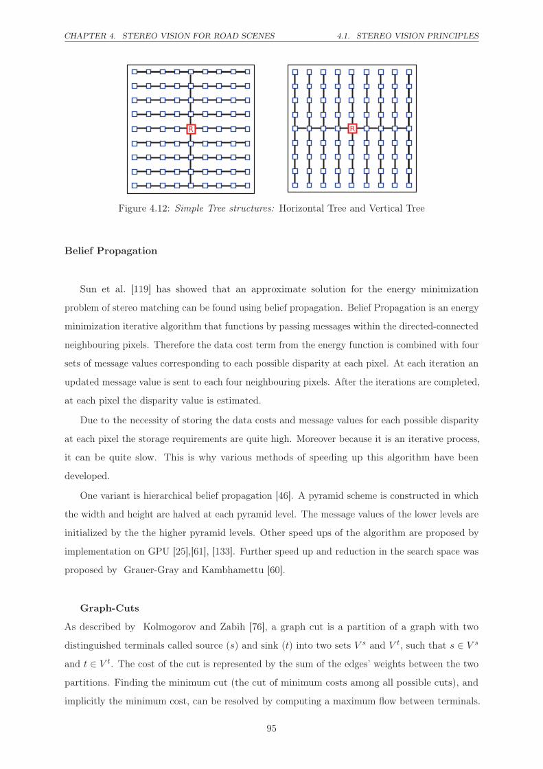
CHAPTER 4. STEREO VISION FOR ROAD SCENES 4.1. STEREO VISION PRINCIPLES
� �
Figure 4.12: Simple Tree structures: Horizontal Tree and Vertical Tree
Belief Propagation
Sun et al. [119] has showed that an approximate solution for the energy minimization
problem of stereo matching can be found using belief propagation. Belief Propagation is an energy
minimization iterative algorithm that functions by passing messages within the directed-connected
neighbouring pixels. Therefore the data cost term from the energy function is combined with four
sets of message values corresponding to each possible disparity at each pixel. At each iteration an
updated message value is sent to each four neighbouring pixels. After the iterations are completed,
at each pixel the disparity value is estimated.
Due to the necessity of storing the data costs and message values for each possible disparity
at each pixel the storage requirements are quite high. Moreover because it is an iterative process,
it can be quite slow. This is why various methods of speeding up this algorithm have been
developed.
One variant is hierarchical belief propagation [46]. A pyramid scheme is constructed in which
the width and height are halved at each pyramid level. The message values of the lower levels are
initialized by the the higher pyramid levels. Other speed ups of the algorithm are proposed by
implementation on GPU [25],[61], [133]. Further speed up and reduction in the search space was
proposed by Grauer-Gray and Kambhamettu [60].
Graph-Cuts
As described by Kolmogorov and Zabih [76], a graph cut is a partition of a graph with two
distinguished terminals called source (s) and sink (t) into two sets V s and V t, such that s ∈ V s
and t ∈ V t. The cost of the cut is represented by the sum of the edges’ weights between the two
partitions. Finding the minimum cut (the cut of minimum costs among all possible cuts), and
implicitly the minimum cost, can be resolved by computing a maximum flow between terminals.
95

4.1. STEREO VISION PRINCIPLES CHAPTER 4. STEREO VISION FOR ROAD SCENES
An example of a minimum cut in a graph is shown in figure 4.13. In practice the global energy
minimisation technique using graph cuts has been shown to be effective with the condition of
having an appropriate cost function.
������
���
� �
�
�
��
������
���
� �
�
�
��
Figure 4.13: Example of a minimum cut in a graph. A cut is represented by all the edges thatlead from the source set to the sink set (as seen in red edges). The sum of these edges representsthe cost of the cut.
Graph cuts can be applied for the algorithm of stereo matching by modelling the pixels in the
image as nodes in the graph. In figure 4.14a is shown an example of such a graph: all the pixels in
the image are represented as nodes and all the nodes on a given level belong to the same disparity.
The edges starting directly from the source or going directly into sink are given an infinite cost.
The vertical edges that can be viewed in figure 4.14a have as weight the cost of matching a pixel
at a certain disparity. In this implementation graph-cuts will output the same result as a local
matching method with winner-takes-all strategy. This is because the smoothness assumption was
not explicitly modelled. In figure 4.14b a smoothness assumption between horizontal pixels is
modelled, thus each horizontal edge will be given a weight that represents the smoothness penalty.
The simplest way to define the smoothness penalty is to assign a user-defined weight wp when
two neighboured pixels have different disparities, and 0 otherwise.
In practice, for the problem of stereo vision, the constructed graph is a three dimensional
structure. If in figure 4.14b each layer represents just one scanline, in figure 4.15 each layer
represents all the pixels in an image. The vertical edges represent the disparity edges, while all
the horizontal edges represent the smoothness assumption.
96

CHAPTER 4. STEREO VISION FOR ROAD SCENES 4.2. STEREO VISION DATASETS
�����
�����
�����
�������
����
������
���
�� �� � �� � �� �� ��
(a)
�����
�����
�����
�������
����
������
���
�� �� � �� � �� �� ��
(b)
Figure 4.14: Graph cuts example on a scanline in stereo vision: a) without smoothness assumption;b) modelling smoothness assumption
������
�����
�����
�����
�����
�����
����
���
Figure 4.15: Graph Cuts applied to stereo vision algorithm.
4.2 Stereo Vision Datasets
There exist several challenging databases for testing the stereo matching algorithms (4.1), from
simulated road scenes like Van Synthetic stereo [123] and EISATS [96], to real road scenes with
97
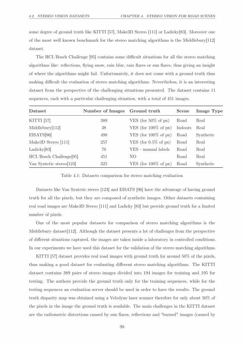
4.2. STEREO VISION DATASETS CHAPTER 4. STEREO VISION FOR ROAD SCENES
some degree of ground truth like KITTI [57], Make3D Stereo [111] or Ladicky[83]. Moreover one
of the most well known benchmark for the stereo matching algorithms is the Middlebury[112]
dataset.
The HCI/Bosch Challenge [95] contains some difficult situations for all the stereo matching
algorithms like: reflections, flying snow, rain blur, rain flares or sun flares, thus giving an insight
of where the algorithms might fail. Unfortunately, it does not come with a ground truth thus
making difficult the evaluation of stereo matching algorithms. Nevertheless, it is an interesting
dataset from the perspective of the challenging situations presented. The dataset contains 11
sequences, each with a particular challenging situation, with a total of 451 images.
Dataset Number of Images Ground truth Scene Image Type
KITTI [57] 389 YES (for 50% of px) Road Real
Middlebury[112] 38 YES (for 100% of px) Indoors Real
EISATS[96] 498 YES (for 100% of px) Road Synthetic
Make3D Stereo [111] 257 YES (for 0.5% of px) Road Real
Ladicky[83] 70 YES - manual labels Road Real
HCI/Bosch Challenge[95] 451 NO Road Real
Van Syntetic stereo[123] 325 YES (for 100% of px) Road Synthetic
Table 4.1: Datasets comparison for stereo matching evaluation
Datasets like Van Syntetic stereo [123] and EISATS [96] have the advantage of having ground
truth for all the pixels, but they are composed of synthetic images. Other datasets containing
real road images are Make3D Stereo [111] and Ladicky [83] but provide ground truth for a limited
number of pixels.
One of the most popular datasets for comparison of stereo matching algorithms is the
Middlebury dataset[112]. Although the dataset presents a lot of challenges from the perspective
of different situations captured, the images are taken inside a laboratory in controlled conditions.
In our experiments we have used this dataset for the validation of the stereo matching algorithms.
KITTI [57] dataset provides real road images with ground truth for around 50% of the pixels,
thus making a good dataset for evaluating different stereo matching algorithms. The KITTI
dataset contains 389 pairs of stereo images divided into 194 images for training and 195 for
testing. The authors provide the ground truth only for the training sequences, while for the
testing sequences an evaluation server should be used in order to have the results. The ground
truth disparity map was obtained using a Velodyne laser scanner therefore for only about 50% of
the pixels in the image the ground truth is available. The main challenges in the KITTI dataset
are the radiometric distortions caused by sun flares, reflections and “burned" images (caused by
98

CHAPTER 4. STEREO VISION FOR ROAD SCENES 4.3. COST FUNCTIONS
strong differences in intensity between light and shadow).
For our experiments we have chosen to work with the last two presented datasets: Middlebury,
due to the considerable number of stereo matching algorithms that have been compared on these
images, and KITTI, in view of our application context.
4.3 Cost functions
The matching cost function measures how "good" a correspondence is. It is important to make a
difference between cost function, cost aggregation and the minimisation methods that use these
costs. A typical classification of the matching costs is: parametric, non-parametric, and mutual
information based costs [67].
4.3.1 Related work
To better understand these categories, they have to be explained in the context of radiometric
distortions. Radiometrical similar pixels refer to those pixels that lie in different images, but in
fact correspond to the same 3D scene point. Thus they should have similar or in a more ideal
case the same intensity values in both images [65]. Radiometrical differences or distortions are
therefore when corresponding pixels have in fact different intensities values. These are caused by:
differences of camera parameters (aperture, sensor) that can induce different image noises and
vignetting; surface properties like non-Lambertian surfaces7; difference in time of acquisition of
the images (like is the case of some satellite imaging).
The parametric costs incorporate the magnitude of pixel intensity. Although usually simple
to compute, the main disadvantage of the parametric costs is that they are often not robust to
radiometric changes. The non-parametric costs incorporate just a local ordering of intensities,
thus it is said that the latter are more reliable to radiometric distortions. The mutual information
(MI) costs are computed on an initial disparity map. MI handles radiometric changes well [49]
but it can only handle radiometric distortions that occur globally thus it has problems to local
radiometric changes (which in practice are more common).
Choosing the right cost function is paramount for having a good disparity map. There exists
several studies where comparison of cost functions is performed, the most extended ones being
made in Hirschmuller and Scharstein [65], Hirschmuller and Scharstein [67]. In comparison with
the study made in 2007, where six cost functions where tested, Hirschmuller and Scharstein [67]
compared fifteen different stereo matching costs in relation with images affected by radiometric
differences. These costs are compared using three different stereo matching algorithms: one
7Lambertian surfaces are the surfaces that reflect the light the same regardless of the observer’s angle of view
99

4.3. COST FUNCTIONS CHAPTER 4. STEREO VISION FOR ROAD SCENES
based on global energy optimisation (Graph Cuts), one using semi-global matching [66] and a
local window-based algorithm. They conclude that the cost based on CT gives the best overall
performance.
In comparison with Hirschmuller and Scharstein [67] that use both simulated and real
radiometric changes in a laboratory environment (Middlebury dataset [112] ), we have chosen for
the experiments to be performed on real road images from the KITTI dataset [57] which presents
significant radiometric differences, as well as the well known Middlebury dataset. Besides the
cost functions that provided the best results in Hirschmuller and Scharstein [67], we also test
some recent functions based on CT that gave good results on the Middlebury dataset8. Moreover
we propose two new cost functions: a fast function similar with the CT called Cross Comparison
Census (CCC) and other function CDiffCensus that remains robust to radiometric changes.
4.3.2 State of the art of matching costs
In the following we present briefly existing cost functions. We divide them in parametric, non-
parametric and mixed parametric costs. We call mixed parametric costs, those costs that try to
enhance the discriminative power of a non-parameteric cost by incorporating extra information
given usually by a parametric cost.
4.3.2.1 Parametric costs.
One of the most popular cost matching function is the squared intensity differences (SD) ( see
equation 4.14) like used by Kolmogorov and Zabih [76] or absolute intensity differences (AD)
(see equation 4.15) which is typically combined with other information like used in Mei et al. [93],
Klaus et al. [75]. SD and AD costs make the assumption of constant color therefore are sensitive
to radiometric distortions.
Let p be a pixel in the left image with coordinates (x, y) and d the disparity value for which
we want to compute the cost of p. Also Il(x, y)i is the intensity value of pixel p in the left image
on color channel i, while Ir(x, y− d)i is the intensity value of pixel given by coordinates (x, y− d)
in the right image. We consider n the number of color channels used ( n = 1 for gray scale images
and n = 3 for color images).
CSD(x, y, d) =1
n
∑
i=1,n
(Il(x, y)i − Ir(x, y − d)i)2; (4.14)
8http://vision.middlebury.edu/stereo/
100

CHAPTER 4. STEREO VISION FOR ROAD SCENES 4.3. COST FUNCTIONS
CAD(x, y, d) =1
n
∑
i=1,n
|Il(x, y)i − Ir(x, y − d)i| (4.15)
If we consider N(x, y) to be the neighbourhood of the pixel with coordinates (x, y), than the
cost AD on this neighbourhood is defined like in equation 4.16. For the CSAD the line between
being a cost function or a cost aggregation technique is very fine.
CSAD(x, y, d) =∑
(a,b)∈N(x,y)
CAD(a, b, d) (4.16)
Filter based parametric costs include algorithms like Laplacian of Gaussian [78], Mean[6],
Bilateral background subtraction [121] which apply a filter on the input images, after which the
matching cost is computed with absolute difference. Other parametric costs that are computed
inside a support window include zero-mean sum of absolute differences(ZSAD), normalized
cross-correlation (NCC) and zero-mean sum of normalized cross-correlation (ZNCC). The ZSAD
subtracts the mean intensity of a support window from each intensity inside that window before
computing the sum of absolute differences. NCC is a parameteric cost that can compensate
for gain changes, while ZNCC is a variant that compensates both gain and offset within the
correlation window [67]. Because ZNCC is a correlation function with values in [0, 1], in order
to obtain the cost we will subtract it from one (see equation 4.17).
CZNCC(x, y, d) = 1− ZNCC(x, y, d) (4.17)
ZNCC(x, y, d) =
∑
(a,b)∈N(x,y)
ZV (Il, a, b)ZV (Ir, a, b− d)
√
∑
(a,b)∈N(x,y)
(ZV (Il, a, b))2∑
(a,b)∈N(x,y)
(ZV (Ir, a, b− d))2(4.18)
ZV (I, x, y) = I(x, y)− IN(x,y)(x, y), (4.19)
where IN(x,y) is the mean value computed in the neighbourhood N(x, y).
In practice the parametric costs have proven to be less robust than the non-parametric ones
[67], [7], with the exception of ZNCC [49],[120].
4.3.2.2 Non-parametric costs.
The most popular non-parametric costs include Rank, Census [136], and Ordinal [17], or pixelwise
costs represented by hierarchical mutual information which were successfully applied by Sarkar
and Bansal [110]. The costs based on gradient or non-parametric measures are more robust to
101

4.3. COST FUNCTIONS CHAPTER 4. STEREO VISION FOR ROAD SCENES
changes in camera gain and bias or non-lambertian surfaces while being less discriminative [75].
CCT . As defined by Zabih and Woodfill [136] to compute the Census Transform (CT ) of
a pixel p a window called the support neighbourhood (n×m), must be centered on each pixel.
Based on this, a bit-string is computed by converting the color values inside the window to value
one, if the corresponding pixel has the value of the color greater than the center pixel’s color value
or zero otherwise. The local intensity relation is given by the equation 4.22, where p1 and p2 are
pixels in the image. The census transform is given by equation 4.21, where ⊗ denotes a bitwise
concatenation and n × m is the census window size. The CT cost is given by the Hamming
distance (DH) between the two bit strings (equation 4.20).
CCT (x, y, d) = DH(CT (x, y), CT (x, y − d)), (4.20)
where CT is the bit string build like in eq. 4.21.
CT (u, v) = ⊗ i=1,nj=1,m
(ξ(I(u, v), I(u+ i, v + j))), (4.21)
where n×m is the census support window, ⊗ denotes a bitwise concatenation, and ξ function is
defined in eq. 4.22.
ξ(p1, p2) =
1 p1 ≤ p2
0 p1 > p2(4.22)
CT can be computed on a dense ( eq. 4.21) or sparse window (eq.4.23). In a sparse window
[70], it is used only every second pixel and every second row as shown in figure 4.16. The filled
blue pixels are the pixels used to compute CT.
CTSparse(u, v) = ⊗i=1:step:n,j=1:step:m(ξ(I(u, v), I(u+ i, v + j))) (4.23)
where step is an empirical chosen value, usually two.
4.3.2.3 Mixed parametric costs.
Non-parametric costs are robust to radiometric distortions but they are less discriminative. That
is why in recent works several combinations between parameteric and non-parameteric costs
are proposed. In what follows we will present these functions. If the authors did not name the
proposed cost functions we are going to use the first name on the article to name the cost.
Cklaus. One of the top three algorithms on the Middlebury dataset [75] proposes the function
Cklaus (equation 4.24) that is a combination between CSAD (equation 4.16) with a gradient based
102
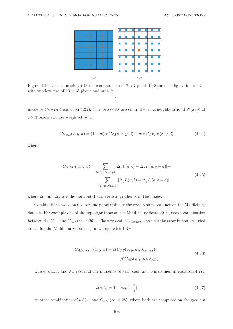
CHAPTER 4. STEREO VISION FOR ROAD SCENES 4.3. COST FUNCTIONS
(a) (b)
Figure 4.16: Census mask: a) Dense configuration of 7× 7 pixels b) Sparse configuration for CTwith window size of 13× 13 pixels and step 2
.
measure CGRAD ( equation 4.25). The two costs are computed in a neighbourhood N(x, y) of
3× 3 pixels and are weighted by w.
Cklaus(x, y, d) = (1− w) ∗ CSAD(x, y, d) + w ∗ CGRAD(x, y, d) (4.24)
where
CGRAD(x, y, d) =∑
(a,b)∈N(x,y)
|∆xIl(a, b)−∆xIr(a, b− d)|+
∑
(a,b)∈N(x,y)
|∆yIl(a, b)−∆yIr(a, b− d)|,(4.25)
where ∆x and ∆y are the horizontal and vertical gradients of the image.
Combinations based on CT became popular due to the good results obtained on the Middlebury
dataset. For example one of the top algorithms on the Middlebury dataset[93], uses a combination
between the CCT and CAD (eq. 4.26 ). The new cost, CADcensus, reduces the error in non-occluded
areas, for the Middlebury dataset, in average with 1.3%.
CADcensus(x, y, d) = ρ(CCT (x, y, d),λcensus)+
ρ(CAD(x, y, d),λAD)(4.26)
where λcensus and λAD control the influence of each cost, and ρ is defined in equation 4.27.
ρ(c,λ) = 1− exp(−c
λ) (4.27)
Another combination of a CCT and CAD (eq. 4.28), where both are computed on the gradient
103

4.3. COST FUNCTIONS CHAPTER 4. STEREO VISION FOR ROAD SCENES
images, is proposed by Stentoumis et al. [114]. It was shown that this new function, Ccstent (
equation 4.28) can give up to 2.5% less erroneous pixels on Middlebury dataset.
Ccstent(x, y, d) = ρ(C∆census(x, y, d),λcensus)+
ρ(CAD(x, y, d),λAD)+
ρ(C∆AD(x, y, d),λ∆AD),
(4.28)
where ∆census and ∆AD are the costs, CT and AD respectively, computed on gradient images.
4.3.3 Motivation: Radiometric distortions
For a stereo matching system to be functional in different conditions, it has to be robust to
radiometrical differences. As previously stated, radiometrical similar pixels refers to those pixels
that correspond to the same scene point and have similar or in an ideal case the same values in
different images [65]. Radiometrical differences or distortions are therefore the situations where
corresponding pixels have different values.
! " # $ % & ' ( ) !*!!!"!#!$!%!&!'!(!)"*"!"""#"$
*
*+!
*+"
*+#
*+$
*+%
*+&
*+'
*+(
*+)
!
,-../01234
56776
89/93 :-;;030<=0
,0><?>.-9@0A3-=:-BA93A-9<CDE
Figure 4.17: The mean percentage of radiometric distortions over the absolute color differencesbetween corresponding pixels in KITTI, respectively Middlebury dataset .
In order to analyse the amount of radiometric distortions in different images, we have compared
the dataset Middlebury and KITTI. In figure 4.17 is presented the mean percentage of radiometric
distortions for the two datasets, over the absolute difference between corresponding pixels. As
stated by Hirschmuller and Scharstein [65], the Middlebury dataset is taken inside a laboratory
in controlled light conditions. Even so, for example at a color absolute difference of five, on the
104

CHAPTER 4. STEREO VISION FOR ROAD SCENES 4.3. COST FUNCTIONS
Figure 4.18: Bit string construction where the arrows show comparison direction for a) CT:‘100001111’, b) CCC: ‘00001111101111110100’ in dense configuration, c) CCC in a sparse configu-ration
Middlebury dataset the average percentage of radiometric distortions is around 28%. On the
other hand on KITTI dataset, where the images were collected outside, the average percentage
of radiometric distortions at the same difference of color is larger than 45%. Therefore it is
important to find a cost function that remains robust to radiometrical distortions.
4.3.4 Contributions
We have proposed two cost functions, one based on a modified CT that has the advantage of a
small computational time while in the same time reducing the error, and the other one based on
a combination between a CT-based cost and a mean sum of differences of intensities that will
provide low errors in radiometrical affected regions.
4.3.4.1 Cross Comparison Census
We propose a new technique to compute the Census Transform bit string, that we named Cross
Comparison Census (CCC). In comparison with CT , the bit string for CCC is obtained by
comparing each pixel in the considered window with those in the immediate vicinity in a clockwise
direction. For comparing the two bit-strings the Hamming distance is used like in the case of CT .
N(i, j, step) = {(i, j + step); (i+ step, j + step);
(i+ step, j); (i+ step, j − step)}(4.29)
where (j + step) < m and (i+ step) < n and (j − step) >= 0
ICCCensus(u, v) = ⊗i=0:step:n,j=0:step:m(ξ(I(i, j), N(i, j, step)) (4.30)
Figure 4.18.a shows the standard CT , while Figure 4.18.b and Figure 4.18.c show the CCC
105

4.3. COST FUNCTIONS CHAPTER 4. STEREO VISION FOR ROAD SCENES
principle in dense configuration and respectively in sparse configuration. The extra information
that is captured in the CCC bit string will result in the possibility of using a smaller window
size and fewer elements in the bit string while keeping all the robust results of the CT or even
improving them.
! " # !$ %& '$ "# $" (! !)) !%! !"" !$# !#$ %%& %&$ %(# '%" '$! "))
)
&
!)
!&
%)
%&
*+
***
,-./0 1230 4 !) 5678"
+2-0590:;<=98
Figure 4.19: Computation time comparison between CT and CCC for different image sizes. Inthe figure an image size of 36 ∗ 104 corresponds to an image of 600× 600 pixels. For both CTand CCC we used a window of 9× 7 pixels, but CCC is computed using a step of two.
CCC can be computed in a very efficient way. First each pixel is compared with those in
the immediate neighbourhood forming a mini bit string which is stored in a matrix. Secondly
the final bit string of a given pixel is formed by the simple concatenation of the mini bit strings
corresponding to the relevant pixels in the census window. These operations remove the redundant
comparisons performed in the CT, making CCC very fast to compute. In the same time this
method is friendly from a hardware perspective because it allows a greater degree of parallelism
than CT. In figure 4.19 it is presented a comparison between computing time of CT and CCC in
a single threaded configuration. It can be observed that when increasing the image size, defined
as the total number of pixels in an image, the computation time for CT has a fast growing rate
while for CCC the computation time increases with a lower rate. The same situation can be
observed in the case of increasing the size of the neighbourhood window. In figure 4.20 we present
comparison between computation time for CT and CCC when increasing the window size while
keeping constant the image size.
4.3.4.2 DiffCensus
We propose a new function that combines the CT [136], or our proposed variant CCC, with
the mean sum of relative differences of intensities inside a window (eq. 4.31). We consider
CCC separately from CT due to its fast computation time. In comparison with functions like
106

CHAPTER 4. STEREO VISION FOR ROAD SCENES 4.3. COST FUNCTIONS
! " ! # " # $ " $ % " % & & " & & & ! " & ! & # " & # & $ " & $
'
#
& '
& #
( '
( #
) *
) ) )
)+,-.- /0,123405+6780"+9-:
)*
)))
!"! #"# $"$ %"% &&"&& &!"&! &#"&# &$"&$
#
&'
&#
('
(#*0;+7-+<2,1-:
Figure 4.20: Computation time comparison between CT and CCC for different neighbourhoodsizes for an image of 1000× 1000 pixels.
CADCensus or Ccstent that use the pixel intensities values, the CDIFFCensus does not rely on the
value of the pixel intensity but on the difference of intensity between a considered pixel and
its neighbourhood. This keeps the function as a non-parametric one while incorporating extra
information.
CDIFFCensus(x, y, d) = ρ(Ccensus(x, y, d),λcensus)+
ρ(CDIFF (x, y, d),λDIFF )(4.31)
where Ccensus can be either CCT , which will give CDIFFCT , or CCCC , which will give CDIFFCCC ;
CDIFF is defined in eq. 4.32.
CDIFF (x, y, d) = |DIFFl(x, y)−DIFFr(x, y − d)| (4.32)
where n ×m is the same support window that is used to compute the CT, and DIFFl is the
DIFF function applied to the left image, while DIFFr is the DIFF function applied to the
right image.
DIFF (u, v) =DIFF (u, v)
CensusSize(4.33)
where CensusSize is the size of the bit string given by the support window n×m and step (eq.
4.29).
107

4.3. COST FUNCTIONS CHAPTER 4. STEREO VISION FOR ROAD SCENES
DIFF (u, v) =∑
i=1:step:nj=1:step:m
(|I(u, v)− I(u+ i, v + j)|), (4.34)
4.3.5 Algorithm
In order to test the proposed cost functions we use two different stereo matching algorithms: one
based on graph cuts, and the other based on local cross aggregation.
4.3.5.1 Graph cuts
As described by Kolmogorov and Zabih [76], a graph cut is a partition of a graph with two
distinguished terminals called source (s) and sink (t) into two sets V s and V t, such that s ∈ V s
and t ∈ V t. The cost of the cut is represented by the sum of the edges’ weights between the
two partitions. Finding the minimum cut, and implicitly the minimum cost, can be resolved
by computing a maximum flow between terminals. In practice the global energy minimisation
technique using graph cuts has been shown to be effective with the condition of having an
appropriate cost function.
For the cost comparison, the energy function is used as described by Kolmogorov and
Zabih [76]. The purpose is to find a disparity function f that minimizes a global energy E(f)
as seen in equation 4.35. The occlusion term Eocc imposes a penalty for occluded pixels, while
Esmooth is the smoothness term which forces neighbouring pixels in the same image to have
similar disparities. The data term Edata(f) measures the cost of matching the function f .
E(f) = Edata(f) + Eocc(f) + Esmooth(f) (4.35)
The data term used by Kolmogorov and Zabih [76] is defined as the cost of squared intensity
differences (CSD). For the following experiments, we will only modify the data term, while
keeping Esmooth and Eocc as defined by Kolmogorov and Zabih [76].
4.3.5.2 Cross-Zones Aggregation & Histogram Voting
For the local technique of energy minimisation we chose to test a cross-based aggregation as
described by Zhang et al. [137]. The algorithm consists in finding for each pixel a cross support
zone. In the first step, a cross is constructed for each pixel. Given a pixel p, its directional arms
(left, right, up or down) are found by applying the following rules:
• Dc(p, pa) < τ . The color difference (Dc) between the pixel p and an arm pixel pa should be
less than a given threshold τ . The color difference is defined as Dc(p, pa) = maxi=1,n|Ii(p)−
108

CHAPTER 4. STEREO VISION FOR ROAD SCENES 4.3. COST FUNCTIONS
Ii(pa)|, where Ii(p) is the color intensity of the pixel p at channel i, and n are the number
of color channels considered.
• Ds(p, pa) < L, where Ds represents the euclidean distance between the pixels p and pa and
L is the maximum length threshold.
Each pixel in the image has a cost given by the considered cost functions. The cost values in
the support region are summed up efficiently using integral images. To select the disparity, the
minimum cost value is selected using a Winner-Take-All strategy. Then a local high-confidence
voting scheme for each pixel is used as described by Lu et al. [90].
4.3.6 Experiments
4.3.6.1 Cost function Parameters
We have optimised each cost function by performing a grid search for the parameters on the first
three images from the KITTI training dataset. For this, we have applied the algorithm of local
stereo matching based on cross zone aggregation. Based on the obtained results, we have found
the parameter values that minimize the error rate as follows:
• CDiffCT : λcensus = 55; λDiff = 95
• CDiffCCC : λcensus = 55; λDiff = 95
• CADcensus: λcensus = 90; λAD = 90
• Cklaus: w = 0.2
• Ccstent: λcensus = 80; λAD = 35; λ∆AD = 80
Figure 4.21 shows the sensitivity of the cost function CDiffCT for the three images, by varying
the parameters λcensus and λDiff , in the interval (0, 100]. Darker values in the figure show smaller
error rate. For the studied function the standard deviation of the error is of 0.52%. The optimised
parameters were use throughout the experiments.
In what concerns the other parameters specific for the two stereo matching algorithms used,
details are given in appendix B, tables B.1 and B.2.
In what follows, we use the KITTI stereo images for all the numerical experiments. KITTI
dataset is divided into 194 images in the training set for which the ground truth images is provided,
and 195 images in the testing set for which an evaluation server should be used in order to obtain
the results. The following experiments are performed only on the 194 images in the training set9
9At the moment of performing the tests, only one submission in 72 hours was allowed on the evaluation server.Thus having an important number of situations to be tested, we have opted to use just the training set.
109

4.3. COST FUNCTIONS CHAPTER 4. STEREO VISION FOR ROAD SCENES
!!"#$
!#"%$
!#"%&
!#"'!
!#"&!
!#"&&
!#"(&
!#"$$
!!"!)
!!")!
!!"*)
!!"+!
!!"%!
!!"%$
!!"'*
!!"&)
!!"&$
!!"(&
!!"$&
!#"&(
!#"*$
!#")$
!#"*#
!#"*'
!#"+%
!#"%+
!#"'!
!#"&+
!#"(#
!#"((
!#"$%
!!"#+
!!"!#
!!"!%
!!")#
!!")(
!!"*%
!!"+*
!#"&%
!#")+
!#"!&
!#"!'
!#"!(
!#"!(
!#")'
!#"*!
!#"*%
!#"+&
!#"%%
!#"'*
!#"&)
!#"(#
!#"((
!#"$+
!#"$(
!!"#)
!!"#&
!#"&%
!#"!&
!#"#*
$"$(
!#"##
!#"#%
!#"!#
!#"!*
!#"!+
!#"!$
!#")%
!#"*!
!#"*(
!#"+*
!#"%!
!#"'#
!#"&#
!#"&&
!#"(#
!#"((
!#"!'
$"$(
$"$!
$"$)
$"$!
$"$&
!#"#+
!#"#'
!#"!#
!#"!*
!#"!(
!#")!
!#")+
!#"*!
!#"*+
!#"*$
!#"+'
!#"%)
!#"$)
!#")#
$"$%
$"(&
$"(+
$"((
$"((
$"($
$"$&
!#"#*
!#"#*
!#"#&
!#"!)
!#"!%
!#"!$
!#"))
!#")'
!#"*#
!#"*+
!#"$'
!#")+
$"$+
$"('
$"(*
$"&$
$"(+
$"((
$"($
$"$*
$"$$
!#"#)
!#"#)
!#"#'
!#"!)
!#"!%
!#"!&
!#")!
!#"))
!#"$$
!#")!
$"$$
$"(!
$"&$
$"&(
$"&'
$"(!
$"(+
$"((
$"((
$"$*
$"$(
!#"##
!#"#)
!#"#%
!#"#(
!#"!!
!#"!*
!!"#+
!#"!&
$"$+
$"()
$"&!
$"&(
$"&%
$"&*
$"&(
$"(#
$"(+
$"(+
$"($
$"$)
$"$$
$"$$
!#"##
!#"#)
!#"#&
!!"!#
!#"!$
$"$%
$"(!
$"&!
$"'$
$"&%
$"&)
$"&)
$"&%
$"&&
$"(!
$"(!
$"('
$"($
$"$)
$"$&
$"$(
$"$$
!!"!&
!#")*
$"$!
$"&&
$"&)
$"'&
$"'(
$"&!
$"&!
$"&!
$"&+
$"&'
$"&(
$"(!
$"(+
$"('
$"$)
$"$)
$"$'
!!")!
!#")%
$"$!
$"&&
$"&!
$"'(
$"'%
$"''
$"'$
$"&!
$"&!
$"&*
$"&%
$"&&
$"(#
$"(!
$"(%
$"(&
$"$!
!!"*#
!#")+
$"$)
$"&+
$"&!
$"''
$"''
$"'*
$"'&
$"''
$"'$
$"'$
$"&!
$"&*
$"&&
$"&(
$"(!
$"(!
$"(+
!!"*&
!#"*)
$"$%
$"&(
$"''
$"'(
$"'*
$"'!
$"')
$"''
$"''
$"'$
$"'$
$"'$
$"&)
$"&&
$"&(
$"(!
$"()
!!"*+
!#"*&
!#"##
$"(#
$"''
$"'&
$"'%
$"')
$"%$
$"%$
$"'%
$"'%
$"'(
$"'(
$"'$
$"&!
$"&%
$"&&
$"&(
!!"*$
!#"*$
!#"#*
$"()
$"'&
$"'*
$"'*
$"'#
$"%$
$"%(
$"'#
$"'%
$"'+
$"''
$"'(
$"'$
$"&!
$"&*
$"&&
!!"+'
!#"+!
!#"#$
$"(+
$"&#
$"'*
$"'+
$"'#
$"%(
$"%'
$"%'
$"'!
$"')
$"'+
$"'%
$"'&
$"'$
$"&#
$"&)
!!"%)
!#"++
!#"!!
$"((
$"&*
$"'+
$"'#
$"'!
$"%(
$"%&
$"%+
$"%%
$"'#
$"'*
$"'*
$"'%
$"''
$"'$
$"&#
!!"%'
!#"+(
!#"!*
$"($
$"&'
$"'(
$"'!
$"%$
$"%(
$"%'
$"%+
$"%'
$"%'
$"%$
$"'#
$"'*
$"'+
$"''
$"'$
!# )# *# +# %# '# &# (# $#
$#
(#
&#
'#
%#
+#
*#
)#
!#
!#"##
!#"%#
!!"##
!!"%#
!!"##
!$%&'('
Figure 4.21: Cost function (CDiffCT ) sensitivity to different parameters values
All the cost functions in this section are evaluated by the average percentage of erroneous pixels
in all zones, occlusions included, and computed at 3 pixels error threshold.
4.3.6.2 Discriminative power of cost functions
In order to quantify how pertinent the information given by each cost function is, we have
compared all the cost functions in relation to all the possible disparities. This is the equivalent
of computing the error rate of stereo matching using only these functions without any cost
aggregation technique. Because some of the cost functions are defined in a neighbourhood, thus
having an advantage in report with the others, we also compute the error given by each function
when using a fixed aggregation window. The results for an error threshold of three pixels are
presented in table 4.2.
Table 4.2: Error percentage of stereo matching with no aggregation (NoAggr) and windowaggregation (WAggr).
Function CAD CSD CCT CADCT CCCC CADCCCCcstent Cklaus CZNCC CDiffCCC CDiffCT
ErrorNoAggr
85.8% 86.22% 71.9% 74.5% 62.3% 71.6% 68.05% 57.52% 39.97% 58.96% 66.51%
ErrorWAggr
42.20% 43.56% 26.92% 23.49% 26.51% 23.49% 27.29% 31.28% 28.68% 22.36% 21.60%
For the cost functions we compare CAD, CSD, CCT with a support window of 7× 9 pixels
(bit string of 63 elements), CCCC with a support window of 7 × 9 pixels and a step of 2 (bit
string of 55 elements), CADCT and CADCCC , Ccstent, Cklaus, CZNCC , CDiffCCC and CDiffCT .
110

CHAPTER 4. STEREO VISION FOR ROAD SCENES 4.3. COST FUNCTIONS
For the results obtained with an aggregation window we have used one of 9× 7 pixels. With no
aggregation and winner takes it all strategy, the most discriminative function is the cost given
by the ZNCC with an error of 39.97%, followed by Cklaus with 57.52%. From the census based
functions, CDiffCCC provides the best results with an error of 58.96% followed by CCCC with
62.3%. The combination of AD with either CT or CCC, overall increases the error rate at 71.9%
and 71.6% respectively. Therefore from a discriminative point of view, CZNCC , Cklaus and CCCC
are the most competitive.
For the results obtained using a window aggregation and winner takes it all strategy, the
proposed function based on mean sum of relative differences provides the best results: CDiffCT
with 21.60%, followed by CDiffCCC with 22.36%. These are followed by the functions based on
ADCensus: CADCT and CADCCC both with 23.49%.
4.3.6.3 Results with graph cuts stereo matching
The graph cuts minimisation algorithm was used as described by Kolmogorov and Zabih [76]
and section 4.3.5.1. Graph cuts minimisation is an iterative process, with the error decreasing
when increasing the number of iterations. One iteration takes around six minutes10 to complete
for an image of size 1241× 376 pixels. We have started the experiments using six iterations but
we did not observed any significant improvement over using just one iteration, while the running
time was considerably increased. Therefore all the experiments presented in this section were
carried out with one iteration.
In order to show the importance of the data term for the energy function, we have tested
the nine cost functions presented in section 4.3.2: CAD, CCensus, CCCCensus, Cklaus, CADcensus,
Ccstent, CZNCC , CDIFFCCC and CDIFFCT . This functions were used without an aggregation
window with the except of Cklaus where a neighbourhood of 3 × 3 pixels is required by the
algorithm and CZNCC where, for the same reasons, a neighbourhood of 9× 7 pixels was used.
Figure 4.22 presents the mean error rate on all the 194 images from the training KITTI
dataset. The error with CSD is quite large, while with the other cost functions the error decreases
significantly. The best overall performance is given by the proposed CDiffCCC function with an
error of 12.26%, followed by CDiffCT with 12.97% and very closely by CZNCC with 12.98%. In
terms of computing time the CZNCC is the slowest function taking in average ten times longer to
compute in comparison with the other two functions.
111

4.3. COST FUNCTIONS CHAPTER 4. STEREO VISION FOR ROAD SCENES
!"!!
#"!!
$!"!!
$#"!!
%!"!!
%#"!!
&!"!!
&#"!!&%"$$
%'"((
$)"(& $("*%$#"'( $'")*
$%"++ $&"!# $%"%(
,-. ,/0123 ,435675 ,8., ,,,, ,,9 ,:;,, ,.<==,9 ,.<==,,,
!"#$%&''('%)*%+,-
*(./%01$2/3($.
Figure 4.22: Mean error for each cost function using graph cuts stereo matching.
!"!!
#"!!
$!"!!
$#"!!
%!"!!
%#"!!
&!"!!
&#"!! &%"'$
%!"'!
$("#&
$#"$$ $)"!) $#"(!
$*"%'
$%"+!$&"+'
,-. ,/0123 ,435675 ,8., ,,,, ,,9 ,:;,, ,.<==,9 ,.<==,,,
!"#$%&''('%)'(**%+,,'-./
0
)(*1%23$415($*
Figure 4.23: Mean error for each cost function using local cross aggregation stereo matching.
4.3.6.4 Local energy optimisation based on cross zone aggregation
Without a real time constraint, the global energy optimisation technique can give very accurate
disparity maps. In comparison, local techniques could achieve real time running with some
trade-off concerning the quality of the disparity map. We have chosen to compare with the global
energy optimisation based on graph cuts a local optimisation based on cross zone aggregation
and local high confidence voting [137] due to the promising results obtained on the Middlebury
[112] dataset.
The same cost functions tested with the graph cuts were evaluated with the local energy
optimisation. The color threshold for cross zone construction used is τ = 20, as chosen by
Zhang et al. [137]. For the maximum arm length two different thresholds were used, vertical arm
Lvertical = 10 and horizontal arm Lhoriz = 17, due to an observed predilection in the considered
dataset of objects to have the same disparity in horizontal. The results obtained on the KITTI
dataset are presented in figure 4.23.
10Our tests were performed on a computer with Dual Core 2.4 GHz single threaded
112

CHAPTER 4. STEREO VISION FOR ROAD SCENES 4.3. COST FUNCTIONS
The overall results are better than those obtained with the graph cuts method (tested in a
reasonable running time situation). When comparing the functions, the best results are obtained
by our proposed functions based on sum of differences: CDiffCCC and CDiffCT . CDiffCT , with
a 12.8% error rate, gives better results than the CDiffCCC , with a 14.07% error rate, but the
latter has a smaller running time of around 40%. The DIFF based functions are followed as
results by the CADCensus and standard CCT based cost functions.
4.3.7 Discussion
Even though the tested cost functions show different discriminative power, as seen in subsection
4.3.6.2 where CCCC has proven to be the most discriminative, a cost aggregation or cost min-
imisation algorithm can change the ranking. For each minimisation method must be chosen a
specific cost function. In figure 4.25 a visualisation of the output disparity map for each function
in combination with the two stereo algorithms is shown. Columns one and three show the results
obtained using the local stereo matching based on cross zone aggregation, while columns two
and four the results obtained with graph cuts. The output results for two images is presented.
While for the first image, results in columns one and two, a satisfactory disparity map is obtained
with both stereo matching algorithms, the second image presented is more challenging due to
large regions without texture. For a better visualisation of the disparity map results, we refer the
reader to appendix C.
For the graph cuts algorithm the proposed CDiffCCC function provided the best results with
very smooth disparity results in the road region but still erroneousness pixels could be found in
textureless areas.
The local stereo matching algorithm gives comparable results with those of graph cuts at
a much lower time cost. In this situation the best results are given by our proposed function
CDiffCT . The disparity map is not as smooth as in the case of the graph cuts algorithm because
we did not used any method of post-filtering. The main problems of the local minimisation
technique based on cross-aggregation lies in big regions of similar color. The assumption when
using an aggregation area is that in the considered region all the pixels have the same disparity.
In practice large areas of same or similar color will not have the same disparity (for example road
region and slanted walls).
Concerning the sensitivity of the cost functions in the presence of radiometric distortions,
distortions quantified as absolute color difference of corresponding pixels, a comparison of different
cost functions is performed (see figure 4.24 ). For this, at each level of radiometric distortion,
for all the 194 images from the training set, the error of the pixels belonging to that level was
113

4.4. CHOOSING THE RIGHT COLOR SPACE CHAPTER 4. STEREO VISION FOR ROAD SCENES
measured. As it can be observed from the figure the proposed cost functions, CDiffCCC and
CDiffCT , give the lowest error rate even in the presence of radiometric distortions.
In what concerns the function behaviour in texture less areas, due to the nature of the function,
it will not improve the results in these regions no more than the other cost function will. For
instance, in a white wall region all the cost functions will not, in general, be able to provide
discriminative values. Therefore it seems that, in texture less areas, the problem does not lay in
the cost function, rather than in the aggregation area or the energy minimisation algorithm used.
! " # $ % & ' ( ) !* !! !" !# !$ !% !& !' !( !) "* "! "" "# "$
*+!
!
,-
...
./
0-.12343
56743
.38128
9:..
-;<<...
-;<<./
=7>?@A18B?C -?38@B8?@23 D0E3@6481 .@6@B -?FF1B12C1G
HBB@B=781
D6@IJ3C761G
Figure 4.24: Output error (logarithmic-scale) for different cost functions in presence of radiometricdistortions
4.4 Choosing the right color space
In the process of stereo matching using grayscale images, ambiguity could arise in situation where
objects of different colors, for example red and green, produce pixels of similar intensities. Thus
intuitively, color should contribute for stereo matching due to the fact that it provides additional
information in comparison with grayscale.
4.4.1 Related work
There exist a few surveys that study the impact of color information in the stereo matching
algorithms. Some studies show that the use of color leads a major improvement by reducing the
error rate like shown in Chambon and Crouzil [28], Okutomi et al. [101], Mühlmann et al. [97]
or Bleyer et al. [21], others by contrary Hirschmuller and Scharstein [67] report that color
114
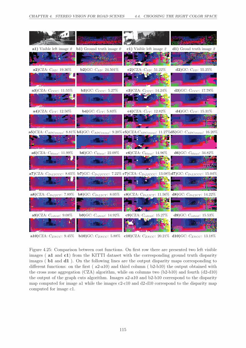
CHAPTER 4. STEREO VISION FOR ROAD SCENES 4.4. CHOOSING THE RIGHT COLOR SPACE
a1) Visible left image 0 b1) Ground truth image 0 c1) Visible left image 2 d1) Groud truth image 2
a2)CZA: CSD: 19.36% b2)GC: CSD: 24.501% c2)CZA: CSD: 51.22% d2)GC: CSD: 55.25%
a3)CZA: CCCC : 11.55% b3)GC: CCCC : 5.27% c3)CZA: CCCC : 14.24% d3)GC: CCCC : 17.78%
a4)CZA: CCT : 12.50% b4)GC: CCT : 5.83% c4)CZA: CCT : 12.82% d4)GC: CCT : 15.31%
a5)CZA: CADCensus: 8.81% b5)GC: CADCensus: 9.20% c5)CZA:CADCensus: 11.27%d5)GC: CADCensus: 16.20%
a6)CZA: Cklaus: 11.99% b6)GC: Cklaus: 22.09% c6)CZA: Cklaus: 14.96% d6)GC: Cklaus: 34.82%
a7)CZA: CDiffCCC : 8.65% b7)GC: CDiffCCC : 7.22% c7)CZA: CDiffCCC : 13.08%d7)GC: CDiffCCC : 15.04%
a8)CZA: CDiffCT : 7.89% b8)GC: CDiffCT : 8.05% c8)CZA: CDiffCT : 11.56% d8)GC: CDiffCT : 14.22%
a9)CZA: Ccstent: 9.08% b9)GC: Ccstent: 14.92% c9)CZA: Ccstent: 15.27% d9)GC: Ccstent: 15.53%
a10)CZA: CZNCC : 9.45% b10)GC: CZNCC : 5.88% c10)CZA: CZNCC : 20.21% d10)GC: CZNCC : 13.18%
Figure 4.25: Comparison between cost functions. On first row there are presented two left visibleimages ( a1 and c1) from the KITTI dataset with the corresponding ground truth disparityimages ( b1 and d1 ). On the following lines are the output disparity maps corresponding todifferent functions: on the first ( a2-a10) and third column ( b2-b10) the output obtained withthe cross zone aggregation (CZA) algorithm, while on columns two (b2-b10) and fourth (d2-d10)the output of the graph cuts algorithm. Images a2-a10 and b2-b10 correspond to the disparitymap computed for image a1 while the images c2-c10 and d2-d10 correspond to the disparity mapcomputed for image c1.
115

4.4. CHOOSING THE RIGHT COLOR SPACE CHAPTER 4. STEREO VISION FOR ROAD SCENES
does not help, especially when using in combination with radiometric insensitive cost functions.
Bleyer and Chambon [19] reports that color has consistently led to performance degradation,
particularly with radiometric insensitive cost functions. Also in [19] there is shown the particular
inefficiency of color stereo matching when the output images from the stereo system present some
color discrepancies.
In the field of autonomous vehicles some stereo matching algorithms using color exist. For
instance Cabani et al. [26] explored color gradient to detect edges in the stereo image pair. The
stereo matching is carried out by computing the photometric distance between the feature point
with its neighbour. This approach remains, however, sensitive to any lighting condition variations
due to a fixed camera gain. In comparison with Cabani et al. [26] and Bleyer and Chambon [19]
, we will combine different color spaces with several stereo matching cost functions using different
stereo matching algorithms.
A color space is an mathematical model that describes different ways in which the colors can
be represented. When acquiring color images, because of the natural outdoors lighting conditions,
the same object may have important discrepancies of color intensities in the stereo image pair.
This makes hard the stereo matching task and hence the disparity computation. In order to
choose an appropriate color space, we will evaluate the error given by the disparity map obtained
using eight different color spaces: RGB, XYZ, LUV, LAB, HLS, YCrCb, HSV and the gray scale
space, as presented in table 4.4.
4.4.2 Experiments
In order to compare different color spaces, we have chosen as database the Middleburry dataset. It
is the only dataset that provides color stereo images along with ground truth values. Performance
of different color spaces can be influenced by the cost function used and also the stereo matching
algorithm. For example the local stereo matching based on cross zones aggregation uses color
thresholds to construct the aggregation region.
For tests we have compared nine different algorithms. In table 4.3 is presented the mean
error rate for each color space and for each cost function across all the algorithms. Results for
individual algorithms across different color spaces and different cost functions are presented in
appendix A.
116

CHAPTER 4. STEREO VISION FOR ROAD SCENES 4.4. CHOOSING THE RIGHT COLOR SPACE
Name Comments
XYZ
X
Y
Z
= 1
0.17697
0.49 0.31 0.20
0.17697 0.81240 0.01063
0 0.01 0.99
R
G
B
LUV L∗ =
{
( 293)3Y/Yn, Y/Y n ≤ ( 6
29)3
116(Y/Yn)1
3 − 16 Y/Y n > ( 6
29)3
where Yn is point luminance
u = 13L ∗ (u′ − u′
n), v = 13L ∗ (v′ − v′n)
where u′ = 4X
X+15Y+3Z, v′ = 9Y
X+15Y+3Z
LAB
L = 116f(Y/Yn)− 16
a = 500[f(X/Xn)− f(Y/Yn)]
b = 200[f(Y/Yn)− f(Z/Zn)
wheref(t) =
{
t1
3 if t > ( 6
29)3
1
3( 29
6)3 + 4
29otherwise
HLS
C = max(R,G,B)−min(R,G,B)
H ′ =
0 if C=0G−B
Cmod6 if M=R
B−R
C+ 2 if M=G
R−G
C+ 4 if M=B
, H = 60◦H ′
L = 1
2(M +m)
S =
{
0 if C=0C
1−|2L−1| otherwise
YCrCb
Y
C
C
=
1/3 1/3 1/3
1 −1/2 −1/2
0 −√3/2
√3/2
R
G
B
HSV
H - similar to H component from HLS
V = max(R,G,B)
S =
{
0 if C=0C
Votherwise
Gray I = 0.3*R+0.59*G+0.11*B
Table 4.4: Color Spaces used for comparison117

4.5. CONCLUSION CHAPTER 4. STEREO VISION FOR ROAD SCENES
RGB XYZ LUV LAB HLS YCrCb HSV GRAY
CSD 26.19 27.09 25.94 26.09 37.28 25.56 37.10 30.51
CAD 24.40 24.54 25.15 25.36 31.93 24.89 30.82 29.57
CCCC 15.81 14.37 21.73 19.87 34.62 21.66 38.93 15.69
CCT 18.12 16.81 23.89 21.88 35.63 23.26 39.51 18.20
CADCT 16.28 15.40 20.09 18.79 27.97 19.53 28.74 16.54
CADCCC 15.01 14.13 19.14 17.83 27.71 18.84 28.49 15.18
CDIFFCT 16.31 15.17 20.48 19.03 30.57 20.20 32.10 15.41
CDIFFCCC 17.60 16.40 21.05 19.98 30.45 20.84 31.22 16.74
Table 4.3: Average error
4.4.3 Discussion
As shown in table 4.3, the color space that consistently provided slightly better results is the
XYZ. Between RGB and GRAY the difference is quite negligible, with the exception of the SD
cost for which the improvement was of 4.3% and AD cost for which the the improvement was of
5.2%. Therefore we back up the claims made by Bleyer and Chambon [19]: in the context of
radiometric insensitive the cost functions the color does not bring an improvement. Nevertheless
it doesn’t degenerate the performance. Moreover, the costs that incorporate some kind of color
information like ADCCC, ADCT, DIFFCT, DIFFCCC, provided better results that the classical
census transform (CT).
We have only tested the performance of different color spaces for stereo matching on the
Middlebury dataset, where images were acquired with the same type of cameras. Further tests
should include color images taken in different conditions with a variety of cameras in order to
insure a diversity that will make the findings statistical relevant.
4.5 Conclusion
In this chapter we have proposed several cost functions robust to radiometric distortions. These
were compared against other state of the art function using two different stereo matching
algorithms: a global method based on graph cuts and a local method based on cross zone
aggregation with high confidence voting.
118

CHAPTER 4. STEREO VISION FOR ROAD SCENES 4.5. CONCLUSION
Experiments show that on KITTI dataset the results of local methods are comparable with
those of global methods. In addition local methods have a high computing speed. From the
tested functions, the proposed function gives the smallest error rate and has proven to be more
robust to radiometric distortions. Consequently, in the context of real time constraint of the
intelligent vehicle application, our choice as a stereo matching algorithm is for the local method
in combination with a cost function based on DIFF (CDiffCT , CDiffCCC).
KITTI dataset for stereovision contains only grayscale information, but color could provide
further discriminative information about the scene, as shown by the experiments performed
Middlebury dataset. Therefore, as future work it would be interesting to test the functions on
color road stereo images.
In the next chapter we are going to study the performance of a multi-modal classifier, Intensity,
Disparity and even Motion, for the task of pedestrian classification. As stereo matching algorithm
for the experiments performed in the next chapter we chose the local stereo matching algorithm
based on cross zone aggregation with high confidence voting and the cost function CDiffCT .
119


5Multi-modality Pedestrian Classification in Visible and FIR
Contents
5.1 Related work . . . . . . . . . . . . . . . . . . . . . . . . . . . . . . . . . 124
5.2 Overview and contributions . . . . . . . . . . . . . . . . . . . . . . . . 125
5.3 Datasets . . . . . . . . . . . . . . . . . . . . . . . . . . . . . . . . . . . . 125
5.4 Preliminaries . . . . . . . . . . . . . . . . . . . . . . . . . . . . . . . . . 127
5.5 Multi-modality pedestrian classification in Visible Domain . . . . . 128
5.5.1 Individual feature classification . . . . . . . . . . . . . . . . . . . . . . . 128
5.5.2 Feature-level fusion . . . . . . . . . . . . . . . . . . . . . . . . . . . . . . 130
5.6 Stereo matching algorithm comparison for pedestrian classification 136
5.7 Multi-modality pedestrian classification in Infrared and Visible Do-
mains . . . . . . . . . . . . . . . . . . . . . . . . . . . . . . . . . . . . . . 138
5.7.1 Individual feature classification . . . . . . . . . . . . . . . . . . . . . . . 139
5.7.2 Feature-level fusion . . . . . . . . . . . . . . . . . . . . . . . . . . . . . . 142
5.8 Conclusions . . . . . . . . . . . . . . . . . . . . . . . . . . . . . . . . . . 142
In the field of pedestrian classification and detection, the main focus was on using the
intensity/color information from the Visible domain. This is proven by the large number
of existing datasets and features developed specifically for the visible domain. Nevertheless,
pedestrian classification in particular, and object classification in general, is still a challenging
problem for computers, whereas for the human perception is a rather easy task. Humans do not
use just the intensity information from the scene, rather employ also cues like depth and motion.
In this chapter we study the performance of different features computed on modalities like
depth and motion, in comparison with the intensity information from Visible domain, along with
different fusion strategies. Moreover, we extend the analysis to the intensity information from
Far Infrared domain.
121

5.1. RELATED WORK CHAPTER 5. MULTI-MODALITY...
5.1 Related work
A new direction of research for pedestrian classification and detection is represented by the
combination of different features and modalities, extracted from Visible Domain, such as intensity,
motion information from optical flow and depth information given by the disparity map.
Visible Domain.
Most of the existing research is using depth and motion just for hypothesis generation, by
constructing a model of the scene geometry. For example, Bajracharya et al. [5] use stereovision
in order to segment the image into regions of interest, followed by the use of geometric features
computed from a 3D point cloud. Enzweiler et al. [38] use motion information in order to extract
region of interest in the image, followed by shape based detection and texture based classification.
Ess et al. [43] integrate stereo depth cues, ground-plane estimation, and appearance-based
object detection. Gavrila and Munder [55] use (sparse) stereo-based ROI generation, shape-
based detection, texture-based classification and (dense) stereo-based verification. Nedevschi
et al. [99] propose a method for object detection and pedestrian hypothesis generation based on
3D information, and use a motion-validation method to eliminate false positives among walking
pedestrians.
Rather than just using depth and motion as cues for the hypothesis generation, a few research
works began integrating features extracted from these modalities directly into the classification
algorithm. For example, Dalal et al. [31] proposed the use of histogram of oriented flow (HOF)
in combination with the well known HOG for human classification. Rohrbach et al. [109]
propose a high level fusion of depth and intensity utilizing not only the depth information in the
pre-processing step, but extracting discriminative spatial features (gradient orientation histograms
and local receptive fields) directly from (dense) depth and intensity images. Both modalities
are represented in terms of individual feature spaces. Wojek et al. [132] incorporates motion
estimation, using HOG, HAAR and Oriented Histograms of Flow. Walk et al. [127] proposed a
combination of HOF and HOG, along with other intensity based features, with very good results
on a challenging monocular dataset: Caltech[36]. Walk et al. [128] proposed the combination
of HOG, HOF, and a HOG-like descriptor applied on the disparity field (HOS), along with a
proposed Disparity statistics (DispStat) feature. Most of these articles have used just one feature
applied on different modalities and they lack an analysis of the performance of different features
computed from a given modality.
Enzweiler et al. [41], [40] proposed a new dataset for pedestrian classification and combine
different modalities, eg. intensity, shape, depth and motion, extracting HOG, LBP and Chamfer
distance features. Moreover they propose a mixture-of-expert framework in order to integrate all
122

CHAPTER 5. MULTI-MODALITY... 5.2. OVERVIEW AND CONTRIBUTIONS
these features.
FIR domain.
In addition of multi-modality fusion in the Visible domain, several studies use Stereovision in the
Far-Infrared domain. For example, Krotosky and Trivedi [81] use a four-camera system (two
visible cameras and two infrared) and compute two dense disparity maps: one in visible and
one in infrared. They use the information from the disparity map through the computation of
v-disparity [82] in order to detect obstacles and generate pedestrian hypothesis. This work is
extended in [80], where HOG-like features are computed on Visible, Infrared and Disparity map
and then fused. Unfortunately, the tests performed by Krotosky and Trivedi [81],[80] were on a
relative small dataset where no other obstacles beside the pedestrians were present.
Bertozzi et al. [14],[11] proposed a system for pedestrian detection in stereo infrared images
based on warm area detection, edge based detection and v-disparity computation. Stereo
information is used just to refine the hypothesis generated and compute the distance and size of
detected objects, but it is not used in the classification process.
5.2 Overview and contributions
In comparison with Enzweiler and Gavrila [40] we extend the analysis of the impact of different
modalities (Intensity, Depth and Motion) in combination with different features, along with
several fusion strategies: between same features but different modalities, different features same
modality, different features different modalities, of "best features" fusion for each modality. All
these results are presented in section 5.5.
Moreover, in section 5.7, we extend the same feature analysis, but this time comparing the
modalities: Far-Infrared, Intensity, Depth and Motion. In addition, we present some insights into
the impact of different stereo vision algorithms for the classification task.
5.3 Datasets
There exists several datasets that are publicly available and commonly used for pedestrian
classification and detection in the visible domain. Table 5.1 presents an overview of existing
datasets in the Visible Domain.
Visible Domain.
INRIA [30] is a well established dataset, but in comparison with newer datasets, it has a
relative small number of people. NICTA dataset [105] consists mostly of images taken with a
digital camera having as training and testing set cropped BB containing people.
123

5.3. DATASETS CHAPTER 5. MULTI-MODALITY...
Data
set
Pro
pertie
sTra
inin
gTestin
g
Acquisition
SetupE
nvironment
Colour
Occlusion
Lab
elStereo
No.
Img.
No.
Ped.
No.
Img.
No.
Ped.
Caltech
[36]M
obileR
oadScene
Yes
Yes
aN
o128
k192k
121k155k
Daim
lerM
onocular[39]
Mobile
Road
SceneN
oN
oN
o-
15560
21790
56.492
Daim
lerM
ulti-Cue
[41]M
obileb
Road
SceneN
oYes
cYes
-52k
-11k
ET
H[43]
Mobile
Sidewalk
Yes
No
Yes
4901
5782
29312k
INR
IA[30]
Photos
-Y
esN
oN
o-
1208
-566
KIT
TI
[57]M
obileR
oadScene
Yes
Yes
Yes
74814487
7518O
nlineE
val-uation
NIC
TA
[105]P
hotosR
oadScene
Yes
Yes
Yes
-18.7k
-6.9k
TU
D-B
russels[132]
Mobile
Road
SceneYes
No
No
1284
1776
5081
498
Parm
aTetravision
Mobile
Road
SceneN
oYes
dYes
1024011554
833811451
Table
5.1:D
atasetscom
parisonfor
pedestrian
classificationand
detection
aC
om
plete
occlu
sion
labels
bOnly
cropped
BB
are
prov
ided
cNon-o
ccluded
and
partia
llyocclu
ded
labels
prov
ided
dJust
two
class
label:
occlu
ded
and
non-o
ccluded
124

CHAPTER 5. MULTI-MODALITY... 5.4. PRELIMINARIES
In comparison with these two datasets, Caltech [36], Daimler Monocular [39], Daimler Multi-
Cue [41] , ETH [43] and KITTI [39] are all captured in an urban scenario with a camera mounted
on a vehicle or stroller ( as in the case of ETH).
Caltech [36] is one of the most challenging monocular databases having a huge number of
annotated pedestrians for both training and testing datasets. Daimler Monocular [39] provides
cropped BB of pedestrians in the training set, but road sequences of images for the testing.
Daimler Multi-Cue [41] is a multi modal dataset that contains cropped pedestrian and non-
pedestrian BB, but with information from visible, depth and motion. ETH [43] is a dataset
acquired mostly on a side walk using a stroller and a stereovision setup, thus it has both
temporal information (images are provided in a sequence) and the possibility of using the disparity
information. KITTI object dataset [57] is a newer dataset that contains stereo images with
annotated pedestrians, cyclists and cars. Although it does not have the possibility of using
temporal information, there is the possibility of using 3D laser data.
Infrared Domain.
Aside from the datasets from the Visible domain, we have considered also the dataset
ParmaTetravision. This contains images from both Visible and Infrared. Moreover the dataset
contains stereo-images, thus making an interesting dataset for comparing different domains and
modalities. An overview of available datasets in Infrared Domain is given in chapter 2.2.
In what follows, we are going to use for the experiments the dataset Daimler Multi-Cue for
Visible domain, and ParmaTetravision for Infrared domain. The reason why we didn’t chose for
Infrared domain RIFIR dataset, is because it does not contain stereo images.
5.4 Preliminaries
Throughout this chapter, for the experiments we are going to use the following configuration:
Classifier. In terms of classifier we have chosen to work with Support Vector Machine. For
this, we have used the library LibLinear[44].
Domains. This chapter contains two major parts: section 5.5 that focuses on Visible domain
and section 5.7 that deals with Far-Infrared domain.
Modalities. As modalities we will study Intensity, from Visible and Infrared domain, and
Depth and Motion computed using the information from the Visible domain.
125

5.5. VISIBLE DOMAIN CHAPTER 5. MULTI-MODALITY...
Features. In terms of features we compare HOG (as presented in section 1.4.1), ISS (as
presented in section 2.3), LBP (as presented in section 1.4.2), LGP (as presented in section 1.4.3),
HaarWavelets (as presented in section 1.4.5) and MSVZM (Mean Scale Value Zero Mean).
In what concerns MSVZM we have implemented a variation based on the feature MSVD
described in section 1.4.6. MSVD is a feature proposed specially for Disparity modality. The
difference between our implementation and the one proposed by Walk et al. [128] is that we
compute a zero-mean and perform L1 normalization, which results in a better performance.
5.5 Multi-modality pedestrian classification in Visible Domain
For the dataset used for the first set of experiments, that of feature comparison for the problem of
pedestrian classification in Visible domain, we have used the dataset Daimler Multi-cue proposed
by Enzweiler et al. [41]. The dataset is publicly available and contains cropped pedestrians
at a dimension of 96 × 48 pixels, along with manually annotated negative examples. It is a
good benchmark for feature comparison in different modalities due to available information from
intensity, flow and disparity.
Pedestrians Pedestrians Non-Pedestrians
(labeled) (jittered)
Train Set 6514 52112 32465
Partially Occluded Test Set 620 11160 16235
Non-Occluded Test Set 3201 25608 16235
Table 5.2: Training and test set statistics for Daimler Multi-Cue Dataset
5.5.1 Individual feature classification
For this experiment, we use each feature independently, HOG, ISS, LBP, LGP, Haar Wavelets
and MSVZM, operating in each modality (intensity, depth or motion).
First of all, we have compared MSVD and MVDZM by drawing the ROC curves corresponding
to the classification of the Daimler non-occluded dataset using only Depth information (see figure
5.1). Based on the ROC curve, at a classification rate of 90%, the false positive rate for MSVD is
of 0.391, while for the MVDZM is of 0.36. Even if we use L1 normalization for MSVD the false
positive rate remains at 0.39 therefore it seems that the process of zero mean lowers the error.
126
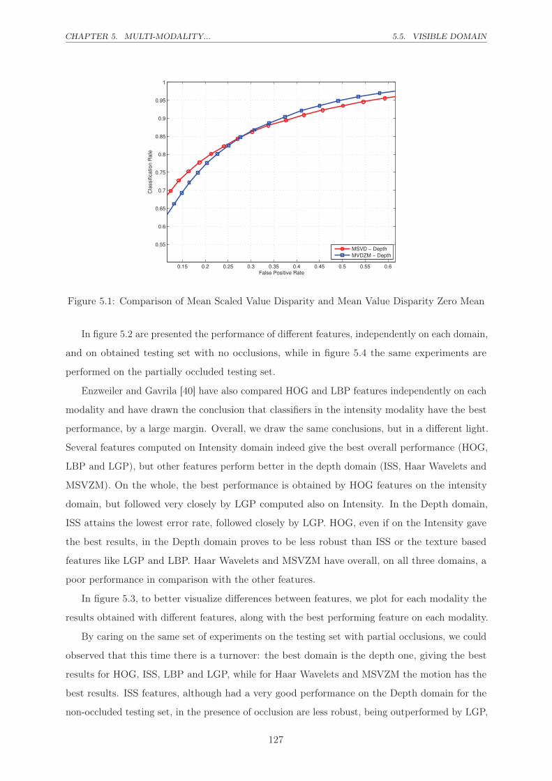
CHAPTER 5. MULTI-MODALITY... 5.5. VISIBLE DOMAIN
0.15 0.2 0.25 0.3 0.35 0.4 0.45 0.5 0.55 0.6
0.55
0.6
0.65
0.7
0.75
0.8
0.85
0.9
0.95
1
False Positive Rate
Cla
ssific
atio
n R
ate
MSVD − Depth
MVDZM − Depth
Figure 5.1: Comparison of Mean Scaled Value Disparity and Mean Value Disparity Zero Mean
In figure 5.2 are presented the performance of different features, independently on each domain,
and on obtained testing set with no occlusions, while in figure 5.4 the same experiments are
performed on the partially occluded testing set.
Enzweiler and Gavrila [40] have also compared HOG and LBP features independently on each
modality and have drawn the conclusion that classifiers in the intensity modality have the best
performance, by a large margin. Overall, we draw the same conclusions, but in a different light.
Several features computed on Intensity domain indeed give the best overall performance (HOG,
LBP and LGP), but other features perform better in the depth domain (ISS, Haar Wavelets and
MSVZM). On the whole, the best performance is obtained by HOG features on the intensity
domain, but followed very closely by LGP computed also on Intensity. In the Depth domain,
ISS attains the lowest error rate, followed closely by LGP. HOG, even if on the Intensity gave
the best results, in the Depth domain proves to be less robust than ISS or the texture based
features like LGP and LBP. Haar Wavelets and MSVZM have overall, on all three domains, a
poor performance in comparison with the other features.
In figure 5.3, to better visualize differences between features, we plot for each modality the
results obtained with different features, along with the best performing feature on each modality.
By caring on the same set of experiments on the testing set with partial occlusions, we could
observed that this time there is a turnover: the best domain is the depth one, giving the best
results for HOG, ISS, LBP and LGP, while for Haar Wavelets and MSVZM the motion has the
best results. ISS features, although had a very good performance on the Depth domain for the
non-occluded testing set, in the presence of occlusion are less robust, being outperformed by LGP,
127

5.5. VISIBLE DOMAIN CHAPTER 5. MULTI-MODALITY...
LBP and HOG. The most robust feature is LGP computed on the Depth domain, by quite a large
margin in comparison with the other considered features. Of course, in order to treat occlusions
there exist better techniques [41],[47], [48], [59], than the holistic one employed here, but our
desired was to test the robustness of each feature across different modalities. Further results on
the partially occluded testing set using different features are presented in appendix F.1.
0 0.2 0.4 0.6 0.8 10
0.2
0.4
0.6
0.8
1
False Positive Rate
Cla
ssif
icati
on
Rate
HOG (Intensity) 0.0122
LGP (Intensity) 0.0129
LBP (Intensity) 0.0153
ISS (Intensity) 0.2287
HaarW (Intensity) 0.5708
MSVZM (Intensity) 0.6206
0 0.1 0.2 0.3 0.4 0.50.5
0.6
0.7
0.8
0.9
1
False Positive Rate
Cla
ssif
icati
on
Rate
ISS (Depth) 0.0745
LGP (Depth) 0.0749
LBP (Depth) 0.0880
HOG (Depth) 0.0998
HaarW (Depth) 0.3818
MSVZM (Depth) 0.3836
a) b)
0 0.2 0.4 0.6 0.8 10
0.2
0.4
0.6
0.8
1
False Positive Rate
Cla
ssif
icati
on
Rate
LGP (Flow) 0.1497
LBP (Flow) 0.1688
HOG (Flow) 0.1896
ISS (Flow) 0.3097
HaarW (Flow) 0.5356
MSVZM (Flow) 0.5957
0 0.1 0.2 0.3 0.4 0.50.5
0.6
0.7
0.8
0.9
1
False Positive Rate
Cla
ssif
icati
on
Rate
HOG (Intensity) 0.0122
ISS (Depth) 0.0745
LGP (Flow) 0.1497
c) d)
Figure 5.3: Individual classification performance comparison of different features in the threemodalities: a) Intensity; b) Depth; c) Motion; d) Best feature on each modality
5.5.2 Feature-level fusion
After having analysed the effect of each modality independently for different features, we now
evaluate the effect of using for a given feature, modality fusion. Results are given in figure 5.5.
For all features, one can always observe an improvement when fusing the information provided by
different modalities.
The best single modality for HOG, LBP and LGP is the Intensity. But, by fusing Depth
and Motion modalities, is obtained a similar performance with that given by Intensity. In what
128
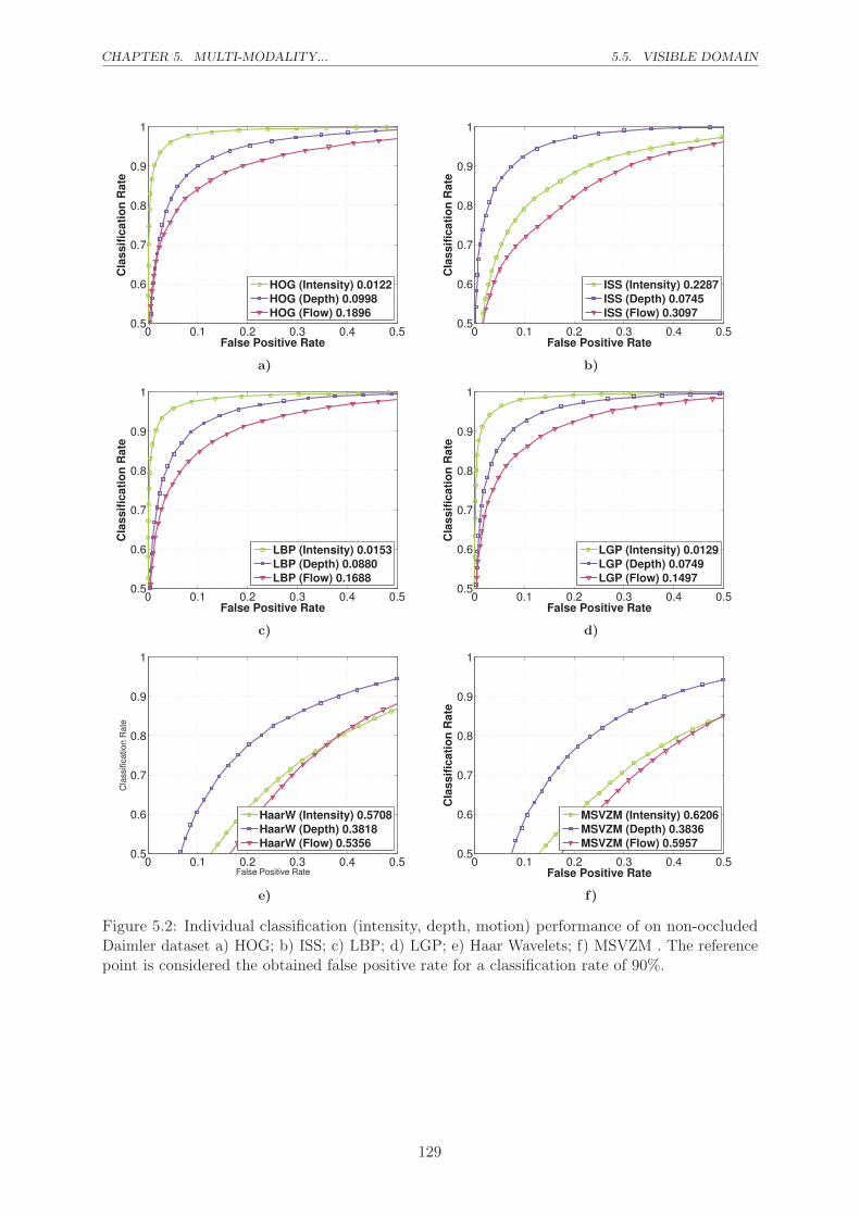
CHAPTER 5. MULTI-MODALITY... 5.5. VISIBLE DOMAIN
0 0.1 0.2 0.3 0.4 0.50.5
0.6
0.7
0.8
0.9
1
False Positive Rate
Cla
ssif
icati
on
Rate
HOG (Intensity) 0.0122
HOG (Depth) 0.0998
HOG (Flow) 0.1896
0 0.1 0.2 0.3 0.4 0.50.5
0.6
0.7
0.8
0.9
1
False Positive Rate
Cla
ssif
icati
on
Rate
ISS (Intensity) 0.2287
ISS (Depth) 0.0745
ISS (Flow) 0.3097
a) b)
0 0.1 0.2 0.3 0.4 0.50.5
0.6
0.7
0.8
0.9
1
False Positive Rate
Cla
ssif
icati
on
Rate
LBP (Intensity) 0.0153
LBP (Depth) 0.0880
LBP (Flow) 0.1688
0 0.1 0.2 0.3 0.4 0.50.5
0.6
0.7
0.8
0.9
1
False Positive Rate
Cla
ssif
icati
on
Rate
LGP (Intensity) 0.0129
LGP (Depth) 0.0749
LGP (Flow) 0.1497
c) d)
0 0.1 0.2 0.3 0.4 0.50.5
0.6
0.7
0.8
0.9
1
False Positive Rate
Cla
ssific
ation R
ate
HaarW (Intensity) 0.5708
HaarW (Depth) 0.3818
HaarW (Flow) 0.5356
0 0.1 0.2 0.3 0.4 0.50.5
0.6
0.7
0.8
0.9
1
False Positive Rate
Cla
ssif
icati
on
Rate
MSVZM (Intensity) 0.6206
MSVZM (Depth) 0.3836
MSVZM (Flow) 0.5957
e) f)
Figure 5.2: Individual classification (intensity, depth, motion) performance of on non-occludedDaimler dataset a) HOG; b) ISS; c) LBP; d) LGP; e) Haar Wavelets; f) MSVZM . The referencepoint is considered the obtained false positive rate for a classification rate of 90%.
129

5.5. VISIBLE DOMAIN CHAPTER 5. MULTI-MODALITY...
0 0.2 0.4 0.6 0.8 10
0.2
0.4
0.6
0.8
1
False Positive Rate
Cla
ssif
icati
on
Rate
HOG (Intensity) 0.6123
HOG (Depth) 0.3132
HOG (Flow) 0.5522
0 0.2 0.4 0.6 0.8 10
0.2
0.4
0.6
0.8
1
False Positive Rate
Cla
ssif
icati
on
Rate
ISS (Intensity) 0.9113
ISS (Depth) 0.5279
ISS (Flow) 0.5371
a) b)
0 0.2 0.4 0.6 0.8 10
0.2
0.4
0.6
0.8
1
False Positive Rate
Cla
ssif
icati
on
Rate
LBP (Intensity) 0.7330
LBP (Depth) 0.4291
LBP (Flow) 0.4581
0 0.2 0.4 0.6 0.8 10
0.2
0.4
0.6
0.8
1
False Positive Rate
Cla
ssif
icati
on
Rate
LGP (Intensity) 0.6487
LGP (Depth) 0.2168
LGP (Flow) 0.5138
c) d)
0 0.2 0.4 0.6 0.8 10
0.2
0.4
0.6
0.8
1
False Positive Rate
Cla
ssific
ation R
ate
HaarW (Intensity) 0.9809
HaarW (Depth) 0.8260
HaarW (Flow) 0.5285
0 0.2 0.4 0.6 0.8 10
0.2
0.4
0.6
0.8
1
False Positive Rate
Cla
ssif
icati
on
Rate
MSVZM (Intensity) 0.9732
MSVZM (Depth) 0.7899
MSVZM (Flow) 0.5772
e) f)
Figure 5.4: Individual classification (intensity, depth, motion) performance on the partial occludedtesting set of a) HOG; b) ISS; c) LBP; d) LGP; e) Haar Wavelets; f) MSVZM
130

CHAPTER 5. MULTI-MODALITY... 5.5. VISIBLE DOMAIN
concerns the other possible fusions per feature, they always provide a smaller false positive rate
than any modality used alone.
As a single modality, Depth always performed better than Motion. When used in combination
with Intensity, the fusion of Intensity and Motion seems to give lower error rate than the
combination Intensity and Depth for the features HOG, LBP and LGP. For ISS features, because
they have a good performance on Depth, the situation is reversed. For the other two considered
features, Haar Wavelets and MSVZM, the fusion of Intensity and Depth also has a better
performance than Intensity and Flow, even if it is at a relative higher overall error.
Fusing Intensity with Depth using a HOG classifier has approximative a factor of 2.6 of less
false positives than a comparable HOG classifier using intensity only; a Intensity and Motion
fusion has a factor of 4.5 less false positives, while all three channels fusion has a factor of
approximative 11 less false positives than the HOG classifier based on Intensity. Taking as
reference the same HOG classifier based on Intensity, the fusion of Depth with Intensity using
LBP based classifier has also a factor of 2.6 less false positives, while an LGP based classifier has
a factor of 3.
Using modality fusion for ISS feature also lowers the error rate in comparison with a single
modality ISS, but the diminishement in the false positive rate is less significant. The same
behaviour is for Haar Wavelets and MSVZM features.
No matter what is the feature employed, the fusion of all three modalities always lowers
the false positive rate. In figure 5.6.a) is showed a comparison of performance when using all
modalities fusion for different features. The best features in term of performance are HOG, LGP
and LBP with a difference in the false positive rate extremely low. These are followed by ISS
feature, but with a factor of approximately ten of higher false positive rate.
While the fusion of all three modalities of HOG feature has the lowest false positive rate at a
classification rate of 90%, the fusion of best feature on each modality seems to be slightly more
robust overall. These results are presented in figure 5.6.b).
In figure 5.7 we compare a classifier based on the best feature on each modality (HOG on
Intensity, ISS on Depth and LGP on Motion), with inter-feature fusion on all modalities. The
best performing system is a classifier trained on four features (HOG, ISS, LGP and LBP) and all
three modalities, having an approximative factor of 50 less positives than a comparable HOG
classifier using Intensity.
131

5.5. VISIBLE DOMAIN CHAPTER 5. MULTI-MODALITY...
0 0.05 0.1 0.15 0.2 0.250.75
0.8
0.85
0.9
0.95
1
False Positive Rate
Cla
ssif
icati
on
Rate
HOG (Intensity) 0.0122
HOG (Intensity+Flow) 0.00271
HOG (Depth+Flow) 0.02827
HOG (Intensity+Depth) 0.00462
HOG (Intensity+Depth+Flow) 0.00117
0 0.05 0.1 0.15 0.2 0.250.75
0.8
0.85
0.9
0.95
1
False Positive Rate
Cla
ssif
icati
on
Rate
ISS (Depth) 0.0745
ISS (Intensity+Flow) 0.08142
ISS (Depth+Flow) 0.02882
ISS (Intensity+Depth) 0.03412
ISS (Intensity+Depth+Flow) 0.01441
a) b)
0 0.02 0.04 0.06 0.08 0.1 0.12
0.88
0.9
0.92
0.94
0.96
0.98
1
False Positive Rate
Cla
ssif
icati
on
Rate
LBP (Intensity) 0.0153
LBP (Intensity+Flow) 0.00234
LBP (Depth+Flow) 0.0185
LBP (Intensity+Depth) 0.00468
LBP (Intensity+Depth+Flow) 0.00172
0 0.02 0.04 0.06 0.08 0.1 0.12
0.88
0.9
0.92
0.94
0.96
0.98
1
False Positive Rate
Cla
ssif
icati
on
Rate
LGP (Intensity) 0.0129
LGP (Intensity+Flow) 0.00209
LGP (Depth+Flow) 0.01903
LGP (Intensity+Depth) 0.00394
LGP (Intensity+Depth+Flow) 0.00154
c) d)
0 0.1 0.2 0.3 0.4 0.50.5
0.6
0.7
0.8
0.9
1
False Positive Rate
Cla
ssif
icati
on
Rate
HaarWave (Depth) 0.3819
HaarWave (Intensity+Flow) 0.3634
HaarWave (Depth+Flow) 0.2368
HaarWave (Intensity+Depth) 0.2854
HaarWave (Intensity+Depth+Flow) 0.1776
0 0.1 0.2 0.3 0.4 0.50.5
0.6
0.7
0.8
0.9
1
False Positive Rate
Cla
ssif
icati
on
Rate
MSVZM (Depth) 0.3836
MSVZM (Intensity+Flow) 0.4149
MSVZM (Depth+Flow) 0.2558
MSVZM (Intensity+Depth) 0.2997
MSVZM (Intensity+Depth+Flow) 0.1997
e) f)
Figure 5.5: Classification performance comparison for each feature using different modality fusion(Intensity+Motion; Depth+Motion; Intensity+Depth; Intensity+Depth+Flow) and the best singlemodality for each feature: a) HOG; b) ISS; c) LBP; d) LGP; e) Haar Wavelets; f) MSVZM.
132
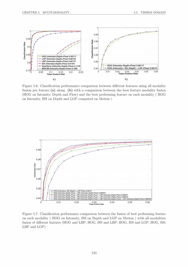
CHAPTER 5. MULTI-MODALITY... 5.5. VISIBLE DOMAIN
0 0.05 0.1 0.15 0.2 0.250.75
0.8
0.85
0.9
0.95
1
False Positive Rate
Cla
ssif
icati
on
Rate
HOG (Intensity+Depth+Flow) 0.00117
LGP (Intensity+Depth+Flow) 0.00154
LBP (Intensity+Depth+Flow) 0.00172
ISS (Intensity+Depth+Flow) 0.01441
HaarWave (Intensity+Depth+Flow) 0.1776
MSVZM (Intensity+Depth+Flow) 0.1997
0 0.01 0.02 0.03 0.04 0.05 0.06
0.94
0.95
0.96
0.97
0.98
0.99
1
False Positive Rate
Cla
ss
ific
ati
on
Ra
te
HOG (Intensity+Depth+Flow) 0.00117
HOG (Intensity)+ ISS (Depth) + LGP (Flow) 0.00141
a) b)
Figure 5.6: Classification performance comparison between different features using all modalityfusion per feature (a) along (b) with a comparison between the best feature modality fusion(HOG on Intensity, Depth and Flow) and the best performing feature on each modality ( HOGon Intensity, ISS on Depth and LGP computed on Motion )
0 0.01 0.02 0.03 0.04 0.05 0.06
0.94
0.95
0.96
0.97
0.98
0.99
1
False Positive Rate
Cla
ss
ific
ati
on
Ra
te
HOG (Intensity)+ ISS (Depth) + LGP (Flow) 0.00141
HOG (Intensity+Depth+Flow) + LBP (Intensity+Depth+Flow) 0.000554
HOG (Intensity+Depth+Flow) + ISS (Intensity+Depth+Flow) + LBP (Intensity+Depth+Flow) 0.000431
HOG (Intensity+Depth+Flow) + ISS (Intensity+Depth+Flow) + LGP (Intensity+Depth+Flow) 0.000616
HOG (Intensity+Depth+Flow) + ISS (Intensity+Depth+Flow) + LBP (Intensity+Depth+Flow) + LGP (Intensity+Depth+Flow) 0.000246
Figure 5.7: Classification performance comparison between the fusion of best performing featureon each modality ( HOG on Intensity, ISS on Depth and LGP on Motion ) with all modalitiesfusion of different features (HOG and LBP; HOG, ISS and LBP; HOG, ISS and LGP; HOG, ISS,LBP and LGP)
133

5.6. STEREO MATCHING... CHAPTER 5. MULTI-MODALITY...
5.6 Stereo matching algorithm comparison for pedestrian classi-
fication
In the same way as different features yield different performance in the classification task, different
stereo matching algorithms can lead to a variation in the error rate for the same feature.
In the previous section, for the experiments performed on Daimler Multi-cue dataset, the
Disparity was pre-computed by the authors using a semi-global matching algorithm [66]. Since
they don’t provide the initial Stereo images, there is no possibility of recomputing the Depth
map using another stereo matching algorithm. Thus, in order to be able to compare different
stereo matching algorithms, we have used as dataset ParmaTetravision.
0 0.2 0.4 0.6 0.8 10
0.2
0.4
0.6
0.8
1
False Positive Rate
Cla
ss
ific
ati
on
Ra
te
HOG (Depth−DiffCensus) 0.1575
HOG (Depth−Geiger) 0.5072
HOG (Depth−ADCensus)0.1730
0 0.2 0.4 0.6 0.8 10
0.2
0.4
0.6
0.8
1
False Positive Rate
Cla
ss
ific
ati
on
Ra
te
ISS (Depth−DiffCensus) 0.2446
ISS (Depth−Geiger) 0.6493
ISS (Depth−ADCensus) 0.2339
a) b)
0 0.2 0.4 0.6 0.8 10
0.2
0.4
0.6
0.8
1
False Positive Rate
Cla
ss
ific
ati
on
Ra
te
LBP (Depth−DiffCensus) 0.1002
LBP (Depth−Geiger) 0.4104
LBP (Depth−ADCensus) 0.1146
0 0.2 0.4 0.6 0.8 10
0.2
0.4
0.6
0.8
1
False Positive Rate
Cla
ss
ific
ati
on
Ra
te
LGP (Depth−DiffCensus) 0.18
LGP (Depth−Geiger) 0.4538
LGP (Depth−ADCensus) 0.1967
c) d)
Figure 5.8: Classification performance comparison of three stereo matching algorithms from theperspective of four features: a) HOG , b) ISS, c) LBP, d) LGP.
Three different Disparity maps were computed on ParmaTetravision using three different
stereo matching algorithms in combination with different features. The purpose of this is to test
if the error difference between these algorithms found in the Disparity map reflects in an error
134

CHAPTER 5. MULTI-MODALITY... 5.6. STEREO MATCHING...
difference when using Depth information for the classification task.
We have chosen the following stereo matching algorithms:
• Local stereo matching based on a cost function of DiffCensus computed in a square window
aggregation and used in combination with cross zone voting (as proposed in chapter 4.3.5.2).
• The same algorithm as described above, but this time just changing the cost function with
ADCensus [93].
• An efficient stereo matching algorithm proposed by Geiger et al. [56], which is based on
triangulation on a set of support points that can be robustly matched. This algorithm
achieved good results on the KITTI dataset, while in the same time has a fast running time.
0 0.2 0.4 0.6 0.8 10
0.2
0.4
0.6
0.8
1
False Positive Rate
Cla
ss
ific
ati
on
Ra
te
HOG (Depth−DiffCensus) 0.1575
ISS (Depth−DiffCensus) 0.2446
LGP (Depth−DiffCensus) 0.18
LBP (Depth−DiffCensus) 0.1002
0 0.2 0.4 0.6 0.8 10
0.2
0.4
0.6
0.8
1
False Positive Rate
Cla
ss
ific
ati
on
Ra
te
HOG (Depth−ADCensus) 0.1730
ISS (Depth−ADCensus) 0.2339
LGP (Depth−ADCensus) 0.1967
LBP (Depth−ADCensus) 0.1146
a) b)
0 0.2 0.4 0.6 0.8 10
0.2
0.4
0.6
0.8
1
False Positive Rate
Cla
ss
ific
ati
on
Ra
te
HOG (Depth−Geiger) 0.5072
ISS (Depth−Geiger) 0.6493
LGP (Depth−Geiger) 0.4538
LBP (Depth−Geiger) 0.4104
c)
Figure 5.9: Classification performance comparison between different features (HOG, ISS, LGP,LBP ) for Depth computed with three different stereo matching algorithms: a) Local stereomatching using DiffCensus cost, b) Local stereo matching using ADCensus cost, c) Stereo matchingusing the algorithm proposed by [56]
The results of comparison in performance of the stereo matching algorithm for different
135
5.7. INFRARED AND VISIBLE CHAPTER 5. MULTI-MODALITY...
features are presented in figure 5.8. Overall, the lowest false positive rate is obtained by the
DiffCensus-based stereo matching algorithm, followed closely by the same algorithm but this time
using as cost function ADCensus. The stereo matching algorithm proposed by Geiger et al. [56]
has a higher false positive rate for all the considered features.
In figure 5.9 we present the same results but in a different light. This time we consider
separately each stereo matching algorithm, and we plot the results obtained with different features
for that algorithm. We can observe that LBP gives consistently a lower error rate for all three
stereo matching algorithms. This is followed by HOG feature in the case of the cross-based stereo
matching using DiffCensus or ADCensus, while for the algorithm proposed by Geiger et al. [56],
LGP gives better results than HOG.
In general the stereo matching algorithm proposed by the Geiger et al. [56] provides slightly
better results than the cross-based algorithm in terms of disparity error1. Nevertheless, due to
the fact that Geiger et al. [56] only considers the robust regions, for the task of classification,
this leads a loss in information in the regions for which is difficult to compute the disparity map.
In the case of the cross-based stereo matching algorithm using DiffCensus or ADCensus, we don’t
disregard the regions for which the disparity map has a high error rate. Thus, in our opinion,
even if we extract features on a disparity map where some errors exist, the classification algorithm
manages to learn and even extract information from these errors.
5.7 Multi-modality pedestrian classification in Infrared and Vis-
ible Domains
In section 2.4 we have presented experiments comparing the visible domain and the far-infrared
domain on two datasets: ParmaTetravision and RIFIR. ParmaTetravision dataset in comparison
with RIFIR, provides information from two visible cameras, therefore the possibility of performing
Stereo matching.
In this section, we extend the experiments on the ParmaTetravision classification dataset, by
evaluating the performance of Depth modality in comparison with Intensity from Visible and
Intensity from FIR domain.
In the same way that we have done the analysis for the Daimler database, we firstly compare
each feature individually on each modality. We have chosen for comparison four features: HOG,
ISS, LBP and LGP and four modalities: Intensity given by Visible Domain, Depth computed
from pair of Visible Stereo Images (using the Stereo matching algorithm based on Cross zone and
1The assessment was done visually, since we don’t have a ground truth for the disparity map
136

CHAPTER 5. MULTI-MODALITY... 5.7. INFRARED AND VISIBLE
DiffCensus cost function - see section 5.6), Motion using Visible images and Intensity values give
by Far-Infrared Domain. The later will be further referenced as simply IR.
For the experiments shown in section 5.7.1 and 5.7.2 we have computed a disparity map based
on the algorithm proposed in chapter 4: for fast computation we employed a square aggregation
window of 7×11 pixels, combined with a voting strategy in a cross window, and a DiffCensus cost
function. In what concerns the dense optical flow algorithm we have used the implementation
provided by Sun et al. [116].
5.7.1 Individual feature classification
In figure 5.10 are presented the performance of each feature on each individual modality. For
each feature, the best performing modality is that of Infrared, followed by Visible and Depth.
The best performing feature on Visible is LBP with a factor of two of less false positives than
a comparable HOG classifier on Visible. This is in comparison with the dataset Daimler, where
HOG had the best performance.
On the Infrared modality, the best performing feature is LGP, followed closely by LBP. HOG
and ISS features on Infrared have also a similar performance but they have a larger error rate:
LGP has a factor of five of less false positives than the comparable HOG classifier on Infrared.
On Depth modality, the best performing feature is LBP, followed this time by HOG. Even if
on Daimler dataset ISS feature had the best results on Depth, on the ParmaTetravision it is not
very robust, having a factor of two more false positives than the LBP.
In what concerns the Motion modality, in comparison with the experiments performed on
Daimler dataset where LGP gave the best results, on these images the best performing feature
was HOG. We believe that this variation in results is given by the quality of the dense optical
flow image obtained. Nevertheless, because of the important difference in performance between
Flow and Intensity modalities, for the fusion of modalities we will consider for now only Infrared
Intensity (IR) , Visible Intensity, and Depth.
137

5.7. INFRARED AND VISIBLE CHAPTER 5. MULTI-MODALITY...
0 0.05 0.1 0.15 0.20.6
0.65
0.7
0.75
0.8
0.85
0.9
0.95
1
False Positive Rate
Cla
ss
ific
ati
on
Ra
te
HOG (Visible) 0.0524
HOG (Depth) 0.1575
HOG (IR) 0.0225
HOG (Flow) 0.2749
0 0.05 0.1 0.15 0.20.6
0.65
0.7
0.75
0.8
0.85
0.9
0.95
1
False Positive Rate
Cla
ss
ific
ati
on
Ra
te
ISS (Visible) 0.0778
ISS (Depth) 0.2446
ISS (IR) 0.0236
ISS (Flow) 0.5565
a) b)
0 0.05 0.1 0.15 0.20.6
0.65
0.7
0.75
0.8
0.85
0.9
0.95
1
False Positive Rate
Cla
ss
ific
ati
on
Ra
te
LBP (Visible) 0.0234
LBP (Depth) 0.1002
LBP (IR) 0.0067
LBP (Flow) 0.3165
0 0.05 0.1 0.15 0.20.6
0.65
0.7
0.75
0.8
0.85
0.9
0.95
1
False Positive Rate
Cla
ss
ific
ati
on
Ra
te
LGP (Visible) 0.0325
LGP (Depth) 0.18
LGP (IR) 0.0042
LGP (Flow) 0.5102
c) d)
Figure 5.10: Individual classification (visible, depth, flow and IR) performance of a) HOG; b)ISS; c) LBP; d) LGP;
138

CHAPTER 5. MULTI-MODALITY... 5.7. INFRARED AND VISIBLE
0 0.05 0.1 0.15 0.20.8
0.85
0.9
0.95
1
False Positive Rate
Cla
ss
ific
ati
on
Ra
te
HOG (IR) 0.0225
HOG (Visible+IR) 0.0042
HOG (Visible+Depth) 0.0325
HOG (IR+Depth) 0.0057
HOG (Visible+Depth+IR) 0.0018
0 0.05 0.1 0.15 0.20.8
0.85
0.9
0.95
1
False Positive Rate
Cla
ss
ific
ati
on
Ra
te
ISS (IR) 0.0236
ISS (Visible+IR) 0.0079
ISS (Visible+Depth) 0.0515
ISS (IR+Depth) 0.0142
ISS (Visible+Depth+IR) 0.0018
a) b)
0 0.05 0.1 0.15 0.20.8
0.85
0.9
0.95
1
False Positive Rate
Cla
ss
ific
ati
on
Ra
te
LBP (IR) 0.0067
LBP (Visible+IR) 0.000540
LBP (Visible+Depth) 0.0109
LBP (IR+Depth) 0.00202
LBP (Visible+Depth+IR) 0.000270
0 0.05 0.1 0.15 0.20.8
0.85
0.9
0.95
1
False Positive Rate
Cla
ss
ific
ati
on
Ra
te
LGP (IR) 0.0325
LGP (Visible+IR) 0.000607
LGP (Visible+Depth) 0.0121
LGP (IR+Depth) 0.000337
LGP (Visible+Depth+IR) 0.00001
c) d)
0 0.05 0.1 0.15 0.20.8
0.85
0.9
0.95
1
False Positive Rate
Cla
ss
ific
ati
on
Ra
te
HOG (Visible+Depth+IR) 0.0018
ISS (Visible+Depth+IR) 0.0018
LBP (Visible+Depth+IR) 0.000270
LGP (Visible+Depth+IR) 0.00001
e)
Figure 5.11: Classification performance comparison for each feature using different modality fusion(Visible+IR; Visible+Depth; IR+Depth; Intensity+Depth+IR) and the best single modality foreach feature: a) HOG; b) ISS; c) LBP; d) LGP. In order to highlight differences between differentfeatures, in e) is plotted for comparison of all modality fusion for different features.
139

5.8. CONCLUSIONS CHAPTER 5. MULTI-MODALITY...
5.7.2 Feature-level fusion
In figure 5.11 we compare for each feature different modality fusions: Visible with Infrared,
Visible and Depth, Infrared and Depth, along with all three modalities fusion: Visible, Depth
and Infrared. The fusion of Visible and Depth lowers the false positive rate for all features in
comparison with the results obtained just on Visible Modality. This result are consistent with the
results obtained on Daimler dataset. Unfortunately, they are still not as good as those obtained
just by the Infrared modality.
Fusing Infrared and Depth on the other hand, lowers the false positive rate in comparison
with just the Infrared modality. For the fusion of Infrared and Depth with HOG feature there is
a factor of approximately of four less false positives than the just the HOG on Infrared. For
ISS, the factor is just of 1.6 and for LBP the factor is of 3.3. The biggest improvement in the
context of fusion of Infrared and Depth, is for LGP feature with a staggering factor of 96 less
false positives than just the LBP feature on Infrared.
The fusion of all three modalities Visible, Infrared and Depth provides the overall best results
for all features. In comparison with Daimler dataset where HOG features had the best results, on
ParmaTetravision HOG and ISS modality fusion have a similar false positive rate. However, the
family of local binary features are much more robust. LBP on Visible, Depth and IR has a factor
of nine less false positives than the similar HOG classifier trained on the same three modalities.
LGP on the other hand has a factor of over 100 less false positives than the HOG classifier.
5.8 Conclusions
In this chapter we have studied the impact of multi-modality (intensity, depth, motion) usage
over the pedestrian classification results. Various features have different performances across
modalities. As single modality, Intensity has the best performance on both tested datasets
(Daimler and ParmaTetravision), followed by Depth. Nevertheless, the fusion of modalities
provides the most robust pedestrian classifier. As single features, local based patterns features
(LGP, LBP) have consistently given robust results, but overall a fusion of complementary features
as well as modalities had the best performance.
Even if the fusion of Intensity and Depth lowers the false positive rate for all features in
comparison with the results obtained just on Intensity in Visible Modality, on the tested dataset,
the Intensity values from the FIR domain had consistently lower error rate. On the other hand, a
fusion between the two domains, FIR and Visible, along with information given by the disparity
map has given the best results on the ParmaTetravision dataset.
140

I think and think for months and years.
Ninety-nine times, the conclusion is false.
The hundredth time I am right.
Albert Einstein
6Conclusion
In this thesis we have focused on the problem of pedestrian detection and classification using
different domains (FIR, SWIR, Visible) and different modalities (Intensity, Motion, Depth Map),
with a particular emphasis on the Disparity map modality.
FIR. We have started by analysing Far-Infrared Spectrum. For this, we have annotated a large
dataset, ParmaTetravision. Because this dataset is not publicly available, we have also acquired a
new dataset called RIFIR. This has allowed us to construct a benchmark in order to analyse the
performance of different features, and in the same time tof compare FIR and Visible spectrums.
Moreover, we have proposed a feature adapted for thermal images, called ISS. Altough ISS has a
similar performance with that of HOG in the far infrared spectrum, local-binary features like
LBP or LGP proved to be more robust. Moreover, in our tests, FIR consistently proved to be
superior to Visible domain. Nevertheless, the fusion between Visible and FIR gave the best
results, lowering the false positive rate with factor of ten in comparison with just using the FIR
domain.
Since one of the main advantages of thermal images is the fact that the search space for
possible pedestrians can be reduced to hot regions in the image, future work should include a
benchmark of ROI extraction algorithms. Moreover, we can extend the feature comparison by
testing different fusion techniques in order to find the most appropriate configuration.
SWIR With the advent of new camera sensors, a promising new domain is represented by Short-
Wave Infrared (SWIR). In this context, we have experimented with two types of cameras. The
preliminary experiments that were performed on a dataset that we have annotated, ParmaSWIR.
This contains images taken using different filters with the purpose of isolation of different
bandwidths. Since the results were promising, we have acquired another dataset, RISWIR, this
time using both a SWIR and a Visible camera. On RISWIR, the short-wave infrared provided
141

CHAPTER 6. CONCLUSION
better results than the Visible one. In our opinion, this is due to the fact that acquired images in
SWIR spectrum are sharper, having well-defined edges.
Further tests in SWIR domain should include different meteorological conditions, along with
an evaluation during night conditions. Moreover, we believe for the results to be conclusive,
SWIR cameras should be compared against several Visible cameras.
StereoVision Since Visible domain represents a low cost alternative to other spectrums, we
give a special attention to Depth modality obtained by constructing the disparity map using
different stereo matching algorithms. In this context, we have worked to improve existing stereo
matching algorithms by proposing new cost function robust to radiometric distortions. As future
work we plan on analysing the impact that post-processing algorithms have over the disparity map.
In addition, in order to incorporate the findings of chapter 5, we should improve the information
contained in the areas subject to occlusions.
Multi-domain, multi-modality. In a similar manner with the way human perception uses
clues given by depth and motion, a new direction of research is the combination of different
modalities and features. A lot of articles tacked this problem from different features point of view
for the Visible domain. Daimler Multi-cue dataset provides a way to centralize this analysis. In
this context we have extended the number of features compared on the dataset with different
modalities, along with several fusion scenarios. The best results were always obtained by fusing
different modalities. Moreover, we extended the analysis multi-modality to a multi-domain
approach, comparing Visible and FIR on ParmaTetravision dataset. Even if the FIR spectrum
continues to give the best results, the fusion between Visible and Depth manages to perform close
to the results given by FIR. Moreover, the fusion between Visible, Depth and FIR lowers the
false positive rate by a factor of thirty, than just the use of FIR information.
As future work, we want to extend the analysis to include more datasets (like ETH [43]), along
with a comparison of different new features. Moreover, in the multi-modalities experiments we
have only treated the problem of pedestrian classification, but we plan of extending the analysis
in a pedestrian detection framework.
There exist various approaches used for the task of pedestrian detection and classification task.
In this thesis, we have showed that a multi-modality, multi-domain approach, and furthermore
multi-feature, is essential for a good pedestrian classification system.
142

AComparison of Color Spaces
Table A.1: Color space comparison using No Aggregation and a Winner takes it all
strategy.
Cost Function RGB XYZ LUV LAB HLS YCrCb HSV GRAY
CSD 66.16 74.94 66.91 67 70.13 66.52 78 75.64
CADCCC 34.76 32.12 43.07 40.35 53.63 43.32 55.94 34.11
CAD 66.57 67.88 67.09 67.28 69.86 66.71 69.11 75.64
CCCC 41.49 37.35 53.49 50.01 63.41 54.55 67.13 40.64
CCT 51.43 48.07 61.49 58.63 68.99 61.9 72.01 51.09
CADCT 42.22 40.01 49.43 47.33 57.68 49.51 59.33 42.65
CDiffCCC 38.77 35.43 47.02 44.36 58.67 48 61.39 36.50
CDiffCT 46.94 43.14 52.73 50.81 63.82 53.67 65.67 42.73
Table A.2: Color space comparison using No Aggregation and Window Voting strategy.
Cost Function RGB XYZ LUV LAB HLS YCrCb HSV GRAY
CSD 30.00 31.7675 32.4208 32.3042 35.1031 31.7288 33.8995 48.17
CADCCC 14.76 13.42 21.8807 20.0289 28.1008 21.4795 29.8935 15.77
CAD 31.21 32.6914 33.4616 33.5808 35.4658 33.0343 34.2492 48.17
CCCC 17.1627 14.90 27.2618 24.4854 37.0718 27.575 42.1272 17.16
CCT 19.7743 17.67 29.8086 27.1517 38.7429 29.9694 43.5671 20.37
CADCT 15.6836 14.45 21.7888 20.1423 27.3889 21.2061 28.984 16.58
CDiffCCC 16.2719 14.60 23.938 22.1868 31.8153 23.5583 34.4055 16.40
CDiffCT 16.7015 15.10 22.817 21.5034 30.8558 22.8666 32.6899 16.69
143

APPENDIX A. COMPARISON OF COLOR SPACES
Table A.3: Color space comparison using No Aggregation and Cross Voting strategy.
Cost Function RGB XYZ LUV LAB HLS YCrCb HSV GRAY
CSD 23.1853 24.6221 23.8924 23.4984 35.6116 21.74 34.5799 43.62
CADCCC 9.8853 9.53 12.0777 11.057 23.8956 11.8662 25.0917 10.26
CAD 25.2124 25.9624 24.8991 24.6209 35.9399 23.36 35.1634 43.62
CCCC 10.8492 9.98 14.0195 12.6536 32.452 14.0836 38.5133 10.35
CCT 13.8631 12.78 18.4191 17.1274 36.3517 17.6975 42.7936 13.76
CADCT 10.6197 10.33 13.0203 11.9332 24.2607 11.8536 25.0075 11.31
CDiffCCC 11.0843 10.47 13.4342 12.2978 27.4328 13.1517 29.6087 10.50
CDiffCT 12.3039 11.28 14.3126 13.553 28.2325 13.6517 29.7005 11.50
Table A.4: Color space comparison using Window Aggregation and Winner take it all
strategy.
Cost Function RGB XYZ LUV LAB HLS YCrCb HSV GRAY
CSD 28.843 26.8752 24.0554 24.6697 45.5687 24.0179 45.0384 22.47
CADCCC 16.3617 15.22 22.4926 20.8911 27.7786 21.7776 28.7909 16.85
CAD 21.56 20.52 22.2395 22.938 27.83 22.2445 26.7601 21.55
CCCC 16.3865 14.55 25.6282 23.1288 35.0064 25.1609 39.2748 16.51
CCT 16.9811 15.27 25.6533 23.0397 34.0793 25.0693 37.9766 17.26
CADCT 16.7156 15.52 22.5112 20.8071 27.5222 21.9147 28.5869 17.13
CDiffCCC 17.2878 15.92 23.7943 22.164 30.5305 23.1127 32.0148 16.77
CDiffCT 17.2317 16.02 22.6881 21.4227 29.0603 22.3661 29.624 17.20
Table A.5: Color space comparison using Window Aggregation and Window Voting strat-
egy.
Cost Function RGB XYZ LUV LAB HLS YCrCb HSV GRAY
CSD 26.135 24.3667 20.9516 21.3165 43.0206 20.7607 42.8491 19.04
CADCCC 14.897 14.09 20.0291 18.7216 24.6324 19.4426 25.3579 15.31
CAD 18.0667 17.20 18.6889 19.1435 23.1094 18.6812 22.1849 18.00
CCCC 14.4862 13.22 22.1633 20.1229 30.6773 21.5609 34.4548 14.62
CCT 14.8307 13.66 21.6604 19.4697 28.9722 20.9686 32.296 14.99
CADCT 14.9334 14.10 19.6912 18.0869 23.8878 19.0941 24.6584 15.14
CDiffCCC 15.668 14.64 21.2967 19.7834 27.1354 20.6203 28.3192 15.13
CDiffCT 15.5516 14.72 20.1489 18.8904 25.4204 19.7925 25.8481 15.36
144

APPENDIX A. COMPARISON OF COLOR SPACES
Table A.6: Color space comparison using Window Aggregation and Cross Voting strategy.
Cost Function RGB XYZ LUV LAB HLS YCrCb HSV GRAY
CSD 12.6762 12.42 12.918 13.0423 21.5226 12.5993 20.6503 12.92
CADCCC 10.8963 10.34 12.7115 11.4688 20.31 12.2459 20.3794 10.99
CAD 12.268 12.13 12.707 12.9205 19.3606 12.4246 18.5638 12.96
CCCC 10.4625 9.66 12.8513 11.6512 25.5045 12.6764 28.9731 10.36
CCT 11.005 10.50 13.7054 11.8693 24.1079 12.7627 26.1566 11.35
CADCT 11.2006 10.74 13.168 11.9889 19.8799 12.2537 20.0019 11.53
CDiffCCC 11.5268 10.75 13.5024 12.1339 22.7681 12.814 23.7329 10.76
CDiffCT 11.7755 11.16 13.8078 12.6727 21.3157 12.977 21.5008 11.62
Table A.7: Color space comparison using Cross Aggregation and Winner Takes it all
strategy.
Cost Function RGB XYZ LUV LAB HLS YCrCb HSV GRAY
CSD 18.7188 18.65 19.503 19.7141 35.7187 19.4803 33.4478 19.89
CADCCC 12.3434 11.86 14.6939 13.8241 27.9153 14.3914 28.259 11.94
CAD 17.1391 16.88 17.495 17.7178 31.9723 17.5203 30.1517 17.37
CCCC 11.9277 11.03 15.7659 14.0439 35.0787 15.1236 40.6607 11.52
CCT 14.2699 13.18 18.4644 16.1716 38.1547 17.039 43.9023 13.63
CADCT 13.1236 12.50 15.4782 14.3622 29.2378 14.8011 29.6902 12.70
CDiffCCC 13.2558 12.6632 15.1867 14.0014 30.1137 14.8062 31.3186 11.67
CDiffCT 14.1111 13.3458 15.9304 15.0104 30.7311 15.586 30.9725 12.99
Table A.8: Color space comparison using Cross Aggregation and Window Voting strategy.
Cost Function RGB XYZ LUV LAB HLS YCrCb HSV GRAY
CSD 15.22 15.3307 16.6239 16.863 24.2304 16.821 22.4271 16.76
CADCCC 10.9851 10.64 13.3125 12.596 21.8262 13.0357 21.6177 10.93
CAD 13.98 13.9967 15.0722 15.2701 21.9465 15.2162 20.5315 14.70
CCCC 10.0924 9.64 13.0713 11.9509 26.597 12.7037 30.164 10.22
CCT 10.878 10.43 13.8252 12.3969 25.7543 12.701 28.6817 10.97
CADCT 11.3643 10.84 13.5748 12.6573 21.0923 12.9682 21.3276 11.15
CDiffCCC 11.8087 11.415 13.8045 12.7777 23.6381 13.5168 24.1776 10.75
CDiffCT 12.348 11.806 14.1029 13.4131 22.3486 13.8942 22.5228 11.62
145

APPENDIX A. COMPARISON OF COLOR SPACES
Table A.9: Color space comparison using Cross Aggregation and Cross Voting strategy.
Cost Function RGB XYZ LUV LAB HLS YCrCb HSV GRAY
CSD 14.77 14.8463 16.2026 16.3635 24.611 16.4097 22.9833 16.11
CADCCC 10.2129 9.92 11.9966 11.5529 21.2961 12.0302 21.0467 10.49
CAD 13.57 13.6026 14.6569 14.809 21.8622 14.8233 20.642 14.11
CCCC 9.41481 8.92 11.3475 10.7914 25.775 11.47 29.0424 9.80
CCT 10.077 9.68 11.9903 11.0646 25.4984 11.2415 28.2317 10.39
CADCT 10.6396 10.08 12.1749 11.8233 20.7813 12.1242 21.0541 10.68
CDiffCCC 11.0808 10.6242 12.3572 11.5996 23.064 12.2227 23.917 10.22
CDiffCT 11.4388 10.9748 12.9124 12.5185 22.282 12.7513 22.4395 10.94
146

BParameters algorithms stereo vision
Parameter Value
Subpixel Computation false
I_threshold1 5
I_threshold2 8
Interaction Radius 6
Lambda 1 15
Lambda 1 5
K 25
Occlusion Penalty 10000
Maximum number of iterations 1
Randomize every iteration true
Table B.1: Parameters Algorithms Graph Cuts
Parameter Value
Arm Length Vertical 10
Arm Length Horizontal 17
Table B.2: Parameters Algorithms Cross Zone Aggregation
147


CDisparity Map image examples
a) Visible left image 0
b) Ground truth image 0
c)CZA: CCT : 12.50%
d)CZA: CDiffCT : 7.89%
Figure C.1: Comparison between cost functions. On first row there are presented the left visibleimage number 0 ( a ) from the KITTI dataset with the corresponding ground truth disparity ( b).On the following lines are the output obtained with the cross zone aggregation (CZA) algorithmwith two different functions: c) Census Tranform; d) the proposed DiffCT
149

APPENDIX C. DISPARITY MAP IMAGE EXAMPLES
a) Visible left image 0
b) Ground truth image 0
c)CZA: CCT : 15.31%
d)CZA: CDiffCT : 14.22%
Figure C.2: Comparison between cost functions. On first row there are presented the left visibleimage number 2 ( a ) from the KITTI dataset with the corresponding ground truth disparity (b). On the following lines are the output obtained with the graph cuts (GC) algorithm with twodifferent functions: c) Census Tranform; d) the proposed DiffCT
150

DCost aggregation
Aggregation area is a very important step for the local algorithms of stereo matching. Global
stereo matching algorithms model in an explicit way the smoothness term (which enforces that
spatially close pixels to have similar disparity). Local algorithms having to model the smoothness
term in an implicit way, the pixels found in the same aggregation area will have a similar disparity.
As presented in subsection 4.1.3.1 there exist a great variety of methods for construction a
cost aggregation area, from the window aggregation areas to adaptive windows or cross-zone
aggregation.
Figure D.1
In section 4.3.5.2 we described the method proposed by Zhang et al. [137]. Mei et al. [93]
proposed an extension for the algorithm of cross-zone aggregation, by using two thresholds for
the maximum area of aggregation:
1. Dc(pl, p) < τ1 and Dc(pl, pl + (1, 0)) < τ1
2. Ds(pl, p) < L1
151

APPENDIX D. COST AGGREGATION
(a) Left Image (b) Ground Truth
(c) Zhang et al. (2009) (7.73%) (d) Mei et al. (2011) (10.58%)
Figure D.2: Different cost aggregation strategies: a) Left Image; b) Disparity Ground Truth; c)Disparity map computed using the strategy proposed by Zhang et al. [137]; d) Disparity mapcomputing using the strategy proposed by Mei et al. [93]
3. Dc(pl, p) < τ2 if L1 < Ds(pl, p) < L2
where L1, L2 are distance thresholds, τ1, τ2 are color thresholds, Dc(pl, p) is a color difference
of two pixels, while Ds(pl, p) is a spatial distance between two pixels.
Based on the above rules, the arms of the cross zones are contructed in the following way:
the first color threshold (τ1) and first size threshold (L1) are used the same way as by Zhang
et al. [137]; in order for the arm to not run across edges a color restriction is enforced between pl
and its predecessor pl + (1, 0) on the same arm; for second size threshold (L2) should be large
enough in order to cover the large textureless areas, but in this case a second color threshold
much more restricive is used (τ2). This strategy gives very good results on the Middlebury dataset
therefore we have tested it on KITTI dataset as well.
Unfortunately, this method of constructing the cross area does not improve the results. The
overall error on the training set from KITTI database is of 21% in comparison with 12.70%
obtained using the strategy of Zhang et al. [137]. We don’t deny the impact of the strategy
proposed by Mei et al. [93] in the textureless areas parallel with the camera plane (see figure
D.2, window area in the right side of the image), but this comes at a higher error rate in the
inclined areas, as that of the road regions.
152
EVoting-based disparity refinement
In section 4.3.5.2 we have briefly presented the cross-based cost aggregation proposed by Zhang
et al. [137]. The initial disparity is selected for each pixel using a Winner Takes-All (WTA)
method. Because the aggregated costs can be usually similar at different disparities, the WTA
will not give very good results. Moreover, WTA strategy has difficulties to handle pixels in the
occluded regions. The refinement scheme proposed by Lu et al. [90] and use also by Zhang
et al. [137] consists in a local voting method.
For every pixel p, having a disparity estimate dp cumputed with WTA, a histogram hp of
disparities is build as showed by equation E.1:
hp(d) =∑
q∈U(p)
δ(dq, d) (E.1)
where U(p) represents the set of all aggregation areas that contain the pixel p, and the function
δ is defined as follows:
δ(da, db) =
1 if da = db
0 otherwise
d∗p = argmax(hp(d)) (E.2)
where d ∈ [0, dmax].
Different from Zhang et al. [137], we propose an extension for the voting algorithm. Due to
the fact that different but close disparities have similar matching costs, the surface of inclined
objects will not appear very smooth. Our proposal is for the voting scheme to not only consider
the disparity dp obtained with WTA, but also the disparities in the interval [dp − v, dp + v].
153

APPENDIX E. VOTING-BASED DISPARITY REFINEMENT
(a) Ground Truth (b) WTA (9.77 %)
(b) Voting Zhang et al. (2011) (7.49%) (c) Our proposed voting (4.50%)
Figure E.1: Different Voting Strategies for the same image
hp(d) =∑
d∈[d−v,d+v]
∑
q∈U(p)
δ(dq, d) (E.3)
Disparity Decision Strategy Error Rate
Winner Takes-All 15.05%
Voting Zhang et al. [137] 12.70%
Proposed Voting (v=2) 10.50%
Table E.1: Comparison of different strategy methods for choosing the disparity
In table E.1 is presented a comparison of obtained error rates on the KITTI dataset using
cross-zone aggregation, the cost CDIFFCF , and three strategies for deciding the final disparity:
WTA, the voting method proposed by Zhang et al. [137], and our proposed voting. It can be
observed that by simply adding the votes to a disparity interval rather than just one disparity
values the error rate decreases with 2.2%.
154

FMulti-modal pedestrian classification
F.1 Daimler-experiments - Occluded dataset
0 0.2 0.4 0.6 0.8 10
0.2
0.4
0.6
0.8
1
False Positive Rate
Cla
ssif
icati
on
Rate
HOG (Intensity) 0.6123
LGP (Intensity) 0.6487
LBP (Intensity) 0.7330
ISS (Intensity) 0.9113
MSVZM (Intensity) 0.9732
HaarW (Intensity) 0.9809
0 0.2 0.4 0.6 0.8 10
0.2
0.4
0.6
0.8
1
False Positive Rate
Cla
ssif
icati
on
Rate
LGP (Depth) 0.2168
HOG (Depth) 0.3132
LBP (Depth) 0.4291
ISS (Depth) 0.5279
MSVZM (Depth) 0.7899
HaarW (Depth) 0.8260
a) b)
0 0.2 0.4 0.6 0.8 10
0.2
0.4
0.6
0.8
1
False Positive Rate
Cla
ssif
icati
on
Rate
LBP (Flow) 0.4581
LGP (Flow) 0.5138
HaarW (Flow) 0.5285
ISS (Flow) 0.5371
HOG (Flow) 0.5522
MSVZM (Flow) 0.5772
0 0.2 0.4 0.6 0.8 10
0.2
0.4
0.6
0.8
1
False Positive Rate
Cla
ssif
icati
on
Rate
HOG (Intensity) 0.6123
LGP (Depth) 0.2168
LBP (Flow) 0.4581
c) d)
Figure F.1: Individual classification performance comparison of different features in the threemodalities for partially occluded testing set: a) Intensity; b) Depth; c) Motion; d) Best feature oneach modality
155
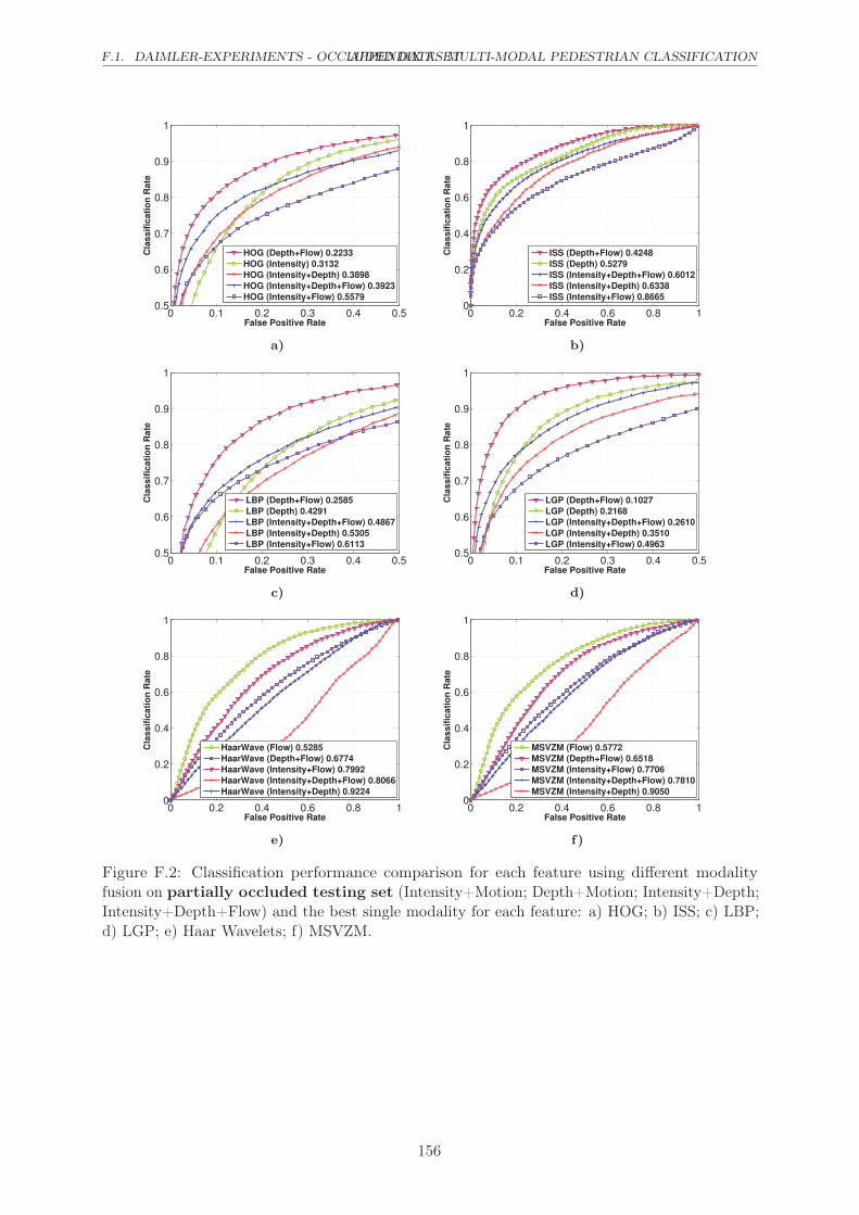
F.1. DAIMLER-EXPERIMENTS - OCCLUDED DATASETAPPENDIX F. MULTI-MODAL PEDESTRIAN CLASSIFICATION
0 0.1 0.2 0.3 0.4 0.50.5
0.6
0.7
0.8
0.9
1
False Positive Rate
Cla
ssif
icati
on
Rate
HOG (Depth+Flow) 0.2233
HOG (Intensity) 0.3132
HOG (Intensity+Depth) 0.3898
HOG (Intensity+Depth+Flow) 0.3923
HOG (Intensity+Flow) 0.5579
0 0.2 0.4 0.6 0.8 10
0.2
0.4
0.6
0.8
1
False Positive Rate
Cla
ssif
icati
on
Rate
ISS (Depth+Flow) 0.4248
ISS (Depth) 0.5279
ISS (Intensity+Depth+Flow) 0.6012
ISS (Intensity+Depth) 0.6338
ISS (Intensity+Flow) 0.8665
a) b)
0 0.1 0.2 0.3 0.4 0.50.5
0.6
0.7
0.8
0.9
1
False Positive Rate
Cla
ssif
icati
on
Rate
LBP (Depth+Flow) 0.2585
LBP (Depth) 0.4291
LBP (Intensity+Depth+Flow) 0.4867
LBP (Intensity+Depth) 0.5305
LBP (Intensity+Flow) 0.6113
0 0.1 0.2 0.3 0.4 0.50.5
0.6
0.7
0.8
0.9
1
False Positive Rate
Cla
ssif
icati
on
Rate
LGP (Depth+Flow) 0.1027
LGP (Depth) 0.2168
LGP (Intensity+Depth+Flow) 0.2610
LGP (Intensity+Depth) 0.3510
LGP (Intensity+Flow) 0.4963
c) d)
0 0.2 0.4 0.6 0.8 10
0.2
0.4
0.6
0.8
1
False Positive Rate
Cla
ssif
icati
on
Rate
HaarWave (Flow) 0.5285
HaarWave (Depth+Flow) 0.6774
HaarWave (Intensity+Flow) 0.7992
HaarWave (Intensity+Depth+Flow) 0.8066
HaarWave (Intensity+Depth) 0.9224
0 0.2 0.4 0.6 0.8 10
0.2
0.4
0.6
0.8
1
False Positive Rate
Cla
ssif
icati
on
Rate
MSVZM (Flow) 0.5772
MSVZM (Depth+Flow) 0.6518
MSVZM (Intensity+Flow) 0.7706
MSVZM (Intensity+Depth+Flow) 0.7810
MSVZM (Intensity+Depth) 0.9050
e) f)
Figure F.2: Classification performance comparison for each feature using different modalityfusion on partially occluded testing set (Intensity+Motion; Depth+Motion; Intensity+Depth;Intensity+Depth+Flow) and the best single modality for each feature: a) HOG; b) ISS; c) LBP;d) LGP; e) Haar Wavelets; f) MSVZM.
156

APPENDIX F. MULTI-MODAL PEDESTRIAN CLASSIFICATIONF.1. DAIMLER-EXPERIMENTS - OCCLUDED DATASET
0 0.1 0.2 0.3 0.4 0.50.5
0.6
0.7
0.8
0.9
1
False Positive Rate
Cla
ss
ific
ati
on
Ra
te
LGP (Depth+Flow) 0.1027
HOG (Depth+Flow) 0.2233
LBP (Depth+Flow) 0.2585
ISS (Depth+Flow) 0.4248
HaarWave (Flow) 0.5285
MSVZM (Flow) 0.5772
Figure F.3: Classification performance comparison on the partially occluded testing sets betweendifferent features using the best modality fusion per feature
0 0.2 0.4 0.6 0.8 10
0.2
0.4
0.6
0.8
1
False Positive Rate
Cla
ss
ific
ati
on
Ra
te
HOG (Intensity+Depth+Flow) 0.3923
ISS (Intensity+Depth+Flow) 0.6012
LBP (Intensity+Depth+Flow) 0.4867
LGP (Intensity+Depth+Flow) 0.2610
HaarWave (Intensity+Depth+Flow) 0.7992
MSVZM (Intensity+Depth+Flow) 0.7810
Figure F.4: Classification performance comparison on the partially occluded testing sets betweendifferent features using the all modality fusion per feature
157


Bibliography
[1] The vislab intercontinental autonomous challenge. http://viac.vislab.it/, 2010.
[2] L. Andreone, F. Bellotti, A. De Gloria, and R. Lauletta. Svm-based pedestrian recognition
on near-infrared images. In Proceedings of the 4th International Symposium on Image and
Signal Processing and Analysis, pages 274–278. IEEE, 2005.
[3] A. Apatean, A. Rogozan, and A. Bensrhair. Objects recognition in visible and infrared
images from the road scene. In IEEE International Conference on Automation, Quality
and Testing, Robotics, 2008, volume 3, pages 327–332, 2008.
[4] Gregory P Asner and David B Lobell. A biogeophysical approach for automated swir
unmixing of soils and vegetation. Remote Sensing of Environment, 74(1):99–112, 2000.
[5] Max Bajracharya, Baback Moghaddam, Andrew Howard, Shane Brennan, and Larry H
Matthies. A fast stereo-based system for detecting and tracking pedestrians from a moving
vehicle. The International Journal of Robotics Research, 28(11-12):1466–1485, 2009.
[6] Emmanuel P Baltsavias and Dirk Stallmann. SPOT stereo matching for Digital Terrain
Model generation. Citeseer, 1993.
[7] Jasmine Banks and Peter Corke. Quantitative evaluation of matching methods and validity
measures for stereo vision. The International Journal of Robotics Research, 20(7):512–532,
2001.
[8] Rodrigo Benenson, Radu Timofte, and Luc Van Gool. Stixels estimation without depth
map computation. In IEEE Conference on Computer Vision Workshops (ICCV Workshops),
pages 2010–2017, 2011.
159

BIBLIOGRAPHY BIBLIOGRAPHY
[9] Rodrigo Benenson, Markus Mathias, Radu Timofte, and Luc Van Gool. Pedestrian detection
at 100 frames per second. In IEEE Conference on Computer Vision and Pattern Recognition
(CVPR), pages 2903–2910, 2012.
[10] M. Bertozzi, A. Broggi, A. Fascioli, T. Graf, and M.M. Meinecke. Pedestrian detection for
driver assistance using multiresolution infrared vision. IEEE Transactions on Vehicular
Technology, 53(6):1666–1678, 2004.
[11] M Bertozzi, A Broggi, A Lasagni, and MD Rose. Infrared stereo vision-based pedestrian
detection. In Intelligent Vehicles Symposium, pages 24–29. IEEE, 2005.
[12] M Bertozzi, A Broggi, M Felisa, G Vezzoni, and M Del Rose. Low-level pedestrian detection
by means of visible and far infra-red tetra-vision. In Intelligent Vehicles Symposium, pages
231–236. IEEE, 2006.
[13] M Bertozzi, A Broggi, C Hilario Gomez, RI Fedriga, G Vezzoni, and M Del Rose. Pedestrian
detection in far infrared images based on the use of probabilistic templates. In Intelligent
Vehicles Symposium, pages 327–332. IEEE, 2007.
[14] Massimo Bertozzi, Emanuele Binelli, Alberto Broggi, and MD Rose. Stereo vision-based
approaches for pedestrian detection. In IEEE Computer Society Conference on Computer
Vision and Pattern Recognition-Workshops, pages 16–16. IEEE, 2005.
[15] Bassem Besbes, Alexandrina Rogozan, and Abdelaziz Bensrhair. Pedestrian recognition
based on hierarchical codebook of surf features in visible and infrared images. In IEEE
Intelligent Vehicles Symposium (IV), pages 156–161, 2010.
[16] Bassem Besbes, Sonda Ammar, Yousri Kessentini, Alexandrina Rogozan, and Abdelaziz
Bensrhair. Evidential combination of svm road obstacle classifiers in visible and far infrared
images. In Intelligent Vehicles Symposium, pages 1074–1079. IEEE, 2011.
[17] Dinkar N. Bhat and Shree K. Nayar. Ordinal measures for image correspondence. IEEE
Transactions on Pattern Analysis and Machine Intelligence, 20(4):415–423, 1998.
[18] E. Binelli, A. Broggi, A. Fascioli, S. Ghidoni, P. Grisleri, T. Graf, and M. Meinecke. A
modular tracking system for far infrared pedestrian recognition. In Intelligent Vehicles
Symposium, pages 759–764. IEEE, 2005.
[19] M. Bleyer and S. Chambon. Does Color Really Help in Dense Stereo Matching? In
Proceedings of the International Symposium on 3D Data Processing, Visualization and
Transmission (3DPVT). Citeseer, 2010.
160

BIBLIOGRAPHY BIBLIOGRAPHY
[20] Michael Bleyer and Margrit Gelautz. Simple but effective tree structures for dynamic
programming-based stereo matching. In International Conference on Computer Vision
Theory and Applications (VISAPP), pages 415–422, 2008.
[21] Michael Bleyer, Sylvie Chambon, Uta Poppe, and Margrit Gelautz. Evaluation of different
methods for using colour information in global stereo matching approaches. Int. Society for
Photogrammetry and Remote Sensing, pages 63–68, 2008.
[22] Alberto Broggi, Massimo Bertozzi, Alessandra Fascioli, and Massimiliano Sechi. Shape-
based pedestrian detection. In Proceedings of the IEEE Intelligent Vehicles Symposium,
pages 215–220. Citeseer, 2000.
[23] Alberto Broggi, Massimo Bertozzi, and Alessandra Fascioli. Self-calibration of a stereo
vision system for automotive applications. In IEEE International Conference on Robotics
and Automation, volume 4, pages 3698–3703, 2001.
[24] Matthew Brown and Sabine Susstrunk. Multi-spectral sift for scene category recognition.
In IEEE Conference on Computer Vision and Pattern Recognition (CVPR), pages 177–184.
IEEE, 2011.
[25] Alan Brunton, Chang Shu, and Gerhard Roth. Belief propagation on the gpu for stereo
vision. In The 3rd Canadian Conference on Computer and Robot Vision, pages 76–76. IEEE,
2006.
[26] I. Cabani, G. Toulminet, and A. Bensrhair. A Fast and Self-adaptive Color Stereo Vision
Matching; a first step for Road Obstacle Detection. In Intelligent Vehicles Symposium,
pages 58–63. IEEE, 2006. ISBN 490112286X.
[27] Pietro Cerri, Luca Gatti, Luca Mazzei, Fabio Pigoni, and Ho Gi Jung. Day and night
pedestrian detection using cascade adaboost system. In 13th International IEEE Conference
on Intelligent Transportation Systems (ITSC), pages 1843–1848. IEEE, 2010.
[28] S. Chambon and A. Crouzil. Colour correlation-based matching. International Journal of
Robotics and Automation, 20(2):78–85, 2005. ISSN 0826-8185.
[29] Corinna Cortes and Vladimir Vapnik. Support-vector networks. Machine learning, 20(3):
273–297, 1995.
[30] Navneet Dalal and Bill Triggs. Histograms of oriented gradients for human detection. In
IEEE Computer Society Conference on Computer Vision and Pattern Recognition, volume 1,
pages 886–893, 2005.
161

BIBLIOGRAPHY BIBLIOGRAPHY
[31] Navneet Dalal, Bill Triggs, and Cordelia Schmid. Human detection using oriented histograms
of flow and appearance. In European Conference on Computer Vision, pages 428–441.
Springer, 2006.
[32] James W Davis and Mark A Keck. A two-stage template approach to person detection in
thermal imagery. In WACV/MOTION, pages 364–369. Citeseer, 2005.
[33] James W Davis and Vinay Sharma. Background-subtraction using contour-based fusion of
thermal and visible imagery. Computer Vision and Image Understanding, 106(2):162–182,
2007.
[34] P. Dollár, Z. Tu, P. Perona, and S. Belongie. Integral channel features. BMVC 2009,
London, England, 2009.
[35] Piotr Dollár, Serge Belongie, and Pietro Perona. The fastest pedestrian detector in the
west. In British Machine Vision Conference, volume 55, 2010.
[36] Piotr Dollar, Christian Wojek, Bernt Schiele, and Pietro Perona. Pedestrian detection: An
evaluation of the state of the art. IEEE Transactions on Pattern Analysis and Machine
Intelligence, 34(4):743–761, 2012.
[37] Nick A Drake, Steve Mackin, and Jeff J Settle. Mapping vegetation, soils, and geology in
semiarid shrublands using spectral matching and mixture modeling of swir aviris imagery.
Remote Sensing of Environment, 68(1):12–25, 1999.
[38] M Enzweiler, P Kanter, and DM Gavrila. Monocular pedestrian recognition using motion
parallax. In Intelligent Vehicles Symposium, pages 792–797. IEEE, 2008.
[39] Markus Enzweiler and Dariu M Gavrila. Monocular pedestrian detection: Survey and
experiments. IEEE Transactions on Pattern Analysis and Machine Intelligence, 31(12):
2179–2195, 2009.
[40] Markus Enzweiler and Dariu M Gavrila. A multilevel mixture-of-experts framework for
pedestrian classification. IEEE Transactions on Image Processing, 20(10):2967–2979, 2011.
[41] Markus Enzweiler, Angela Eigenstetter, Bernt Schiele, and Dariu M Gavrila. Multi-cue
pedestrian classification with partial occlusion handling. In Conference on Computer Vision
and Pattern Recognition (CVPR), pages 990–997. IEEE, 2010.
[42] S Erturk. Region of interest extraction in infrared images using one-bit transform. Signal
Processing Letters, 2013.
162

BIBLIOGRAPHY BIBLIOGRAPHY
[43] Andreas Ess, Bastian Leibe, and Luc Van Gool. Depth and appearance for mobile scene
analysis. In IEEE 11th International Conference on Computer Vision, pages 1–8. IEEE,
2007.
[44] Rong-En Fan, Kai-Wei Chang, Cho-Jui Hsieh, Xiang-Rui Wang, and Chih-Jen Lin. Liblinear:
A library for large linear classification. The Journal of Machine Learning Research, 9:
1871–1874, 2008.
[45] Yajun Fang, Keiichi Yamada, Yoshiki Ninomiya, Berthold Horn, and Ichiro Masaki. Com-
parison between infrared-image-based and visible-image-based approaches for pedestrian
detection. In Intelligent Vehicles Symposium, pages 505–510. IEEE, 2003.
[46] Pedro F Felzenszwalb and Daniel P Huttenlocher. Efficient belief propagation for early
vision. International journal of computer vision, 70(1):41–54, 2006.
[47] Pedro F. Felzenszwalb, Ross B. Girshick, and David McAllester. Cascade object detection
with deformable part models. In IEEE Conference on Computer Vision and Pattern
Recognition, pages 2241–2248, 2010.
[48] Pedro F. Felzenszwalb, Ross B. Girshick, David McAllester, and Deva Ramanan. Object
detection with discriminatively trained part-based models. IEEE Transanctions on Pattern
Analysis and Machine Intelligence, 32(9):1627–1645, 2010.
[49] Clinton Fookes, A Maeder, Sridha Sridharan, and Jamie Cook. Multi-spectral stereo image
matching using mutual information. In 2nd International Symposium on 3D Data Processing,
Visualization and Transmission, pages 961–968. IEEE, 2004.
[50] The Royal Society for the Prevention of Accidents. What are the most common causes
of road accidents? http://www.rospa.com/faqs/detail.aspx?faq=298, 2013. Accessed:
2013-12-03.
[51] D.A. Forsyth and J. Ponce. Computer vision: a modern approach. Prentice Hall Professional
Technical Reference, 2002.
[52] Yoav Freund and Robert E Schapire. A decision-theoretic generalization of on-line learning
and an application to boosting. Journal of computer and system sciences, 55(1):119–139,
1997.
[53] Andrea Fusiello, Vito Roberto, and Emanuele Trucco. Efficient stereo with multiple
windowing. In IEEE Conference on Computer Vision and Pattern Recognition, pages
858–863, 1997.
163

BIBLIOGRAPHY BIBLIOGRAPHY
[54] Tarak Gandhi and Mohan M Trivedi. Pedestrian protection systems: Issues, survey, and
challenges. IEEE Transactions on Intelligent Transportation Systems, 8(3):413–430, 2007.
[55] Dariu M Gavrila and Stefan Munder. Multi-cue pedestrian detection and tracking from a
moving vehicle. International journal of computer vision, 73(1):41–59, 2007.
[56] Andreas Geiger, Martin Roser, and Raquel Urtasun. Efficient large-scale stereo matching.
In Asian Conference of Computer Vision, pages 25–38. Springer, 2011.
[57] Andreas Geiger, Philip Lenz, and Raquel Urtasun. Are we ready for autonomous driving?
the kitti vision benchmark suite. In Computer Vision and Pattern Recognition (CVPR),
Providence, USA, June 2012.
[58] David Geronimo, Antonio M Lopez, Angel Domingo Sappa, and Thorsten Graf. Survey
of pedestrian detection for advanced driver assistance systems. Transactions on Pattern
Analysis and Machine Intelligence, 32(7):1239–1258, 2010.
[59] Ross B Girshick, Pedro F Felzenszwalb, and David A Mcallester. Object detection with
grammar models. In Advances in Neural Information Processing Systems, pages 442–450,
2011.
[60] Scott Grauer-Gray and Chandra Kambhamettu. Hierarchical belief propagation to reduce
search space using cuda for stereo and motion estimation. In Workshop on Applications of
Computer Vision (WACV), pages 1–8. IEEE, 2009.
[61] Scott Grauer-Gray, Chandra Kambhamettu, and Kannappan Palaniappan. Gpu implemen-
tation of belief propagation using cuda for cloud tracking and reconstruction. In IAPR
Workshop on Pattern Recognition in Remote Sensing, pages 1–4. IEEE, 2008.
[62] Erico Guizzo. How Google’s Self-Driving Car Works.
http://spectrum.ieee.org/automaton/robotics/artificial-intelligence/how-google-self-
driving-car-works, Retrieved 18 October 1011.
[63] Marc P Hansen and Douglas S Malchow. Overview of swir detectors, cameras, and
applications. In SPIE Defense and Security Symposium, pages 69390I–69390I. International
Society for Optics and Photonics, 2008.
[64] Simon Hermann and Reinhard Klette. Iterative semi-global matching for robust driver
assistance systems. In Proc. Asian Conf. Computer Vision, LNCS, 2012.
164

BIBLIOGRAPHY BIBLIOGRAPHY
[65] H. Hirschmuller and D. Scharstein. Evaluation of cost functions for stereo matching. In
IEEE Conference on Computer Vision and Pattern Recognition, pages 1–8, 2007. ISBN
1424411807.
[66] Heiko Hirschmuller. Stereo processing by semiglobal matching and mutual information.
IEEE Transactions on Pattern Analysis and Machine Intelligence, 30(2):328–341, 2008.
[67] Heiko Hirschmuller and Daniel Scharstein. Evaluation of stereo matching costs on im-
ages with radiometric differences. IEEE Transactions on Pattern Analysis and Machine
Intelligence, 31(9):1582–1599, 2009.
[68] Heiko Hirschmüller, Peter R Innocent, and Jon Garibaldi. Real-time correlation-based
stereo vision with reduced border errors. International Journal of Computer Vision, 47
(1-3):229–246, 2002.
[69] Asmaa Hosni, Michael Bleyer, Margrit Gelautz, and Christoph Rhemann. Local stereo
matching using geodesic support weights. In 16th IEEE International Conference on Image
Processing (ICIP), pages 2093–2096, 2009.
[70] M. Humenberger, C. Zinner, M. Weber, W. Kubinger, and M. Vincze. A fast stereo
matching algorithm suitable for embedded real-time systems. Computer Vision and Image
Understanding, 2010. ISSN 1077-3142.
[71] Sensors Inc. Why swir? what is the value of shorwave infrared? http://www.sensorsinc.
com/whyswir.html, 2013. Accessed: 2013-10-12.
[72] Bongjin Jun, Inho Choi, and Daijin Kim. Local transform features and hybridization
for accurate face and human detection. Transactions on Pattern Analysis and Machine
Intelligence, pages 1423–1436, 2013.
[73] DS Kim and KH Lee. Segment-based region of interest generation for pedestrian detection
in far-infrared images. Infrared Physics & Technology, 61:120–128, 2013.
[74] DS Kim, M Kim, BS Kim, and KH Lee. Histograms of local intensity differences for
pedestrian classification in far-infrared images. Electronics Letters, 49(4):258–260, 2013.
[75] Andreas Klaus, Mario Sormann, and Konrad Karner. Segment-based stereo matching using
belief propagation and a self-adapting dissimilarity measure. In Proceedings of the 18th
International Conference on Pattern Recognition - Volume 03, ICPR ’06, pages 15–18. IEEE
Computer Society, 2006. ISBN 0-7695-2521-0.
165

BIBLIOGRAPHY BIBLIOGRAPHY
[76] Vladimir Kolmogorov and Ramin Zabih. Computing visual correspondence with occlusions
using graph cuts. In 8th IEEE International Conference on Computer Vision, volume 2,
pages 508–515, 2001.
[77] J.Z. Kolter, Y. Kim, and A.Y. Ng. Stereo vision and terrain modeling for quadruped robots.
In IEEE International Conference on Robotics and Automation, 2009, pages 1557–1564.
IEEE, 2009.
[78] Kurt Konolige. Small vision systems: Hardware and implementation. In ROBOTICS
RESEARCH-INTERNATIONAL SYMPOSIUM-, volume 8, pages 203–212. MIT PRESS,
1998.
[79] Sebastien Kramm and Abdelaziz Bensrhair. Obstacle detection using sparse stereovision
and clustering techniques. In Intelligent Vehicles Symposium (IV), pages 760–765. IEEE,
2012.
[80] Stephen J Krotosky and Mohan M Trivedi. On color-, infrared-, and multimodal-stereo
approaches to pedestrian detection. IEEE Transactions on Intelligent Transportation
Systems, 8(4):619–629, 2007.
[81] Stephen J Krotosky and Mohan M Trivedi. A comparison of color and infrared stereo
approaches to pedestrian detection. In Intelligent Vehicles Symposium, pages 81–86. IEEE,
2007.
[82] Raphael Labayrade, Didier Aubert, and J-P Tarel. Real time obstacle detection in stereovi-
sion on non flat road geometry through" v-disparity" representation. In Intelligent Vehicle
Symposium, 2002. IEEE, volume 2, pages 646–651. IEEE, 2002.
[83] Lubor Ladicky, Paul Sturgess, Chris Russell, Sunando Sengupta, Yalin Bastanlar, William
Clocksin, and Philip HS Torr. Joint optimization for object class segmentation and dense
stereo reconstruction. International Journal of Computer Vision, pages 1–12, 2012.
[84] Bastian Leibe, Edgar Seemann, and Bernt Schiele. Pedestrian detection in crowded scenes. In
IEEE Computer Society Conference on Computer Vision and Pattern Recognition, volume 1,
pages 878–885, 2005.
[85] Guoliang Li, Yong Zhao, Daimeng Wei, and Ruzhong Cheng. Nighttime pedestrian detection
using local oriented shape context descriptor. In Proceedings of the 2nd International
Conference on Computer Science and Electronics Engineering. Atlantis Press, 2013.
166
BIBLIOGRAPHY BIBLIOGRAPHY
[86] J. Li, W. Gong, W. Li, and X. Liu. Robust pedestrian detection in thermal infrared imagery
using the wavelet transform. Infrared Physics & Technology, 53(4):267–273, 2010.
[87] Rainer Lienhart and Jochen Maydt. An extended set of haar-like features for rapid object
detection. In International Conference on Image Processing, volume 1, pages I–900. IEEE,
2002.
[88] Qiong Liu, Jiajun Zhuang, and Jun Ma. Robust and fast pedestrian detection method for
far-infrared automotive driving assistance systems. Infrared Physics & Technology, 2013.
[89] David G Lowe. Distinctive image features from scale-invariant keypoints. International
journal of computer vision, 60(2):91–110, 2004.
[90] Jiangbo Lu, Gauthier Lafruit, and Francky Catthoor. Anisotropic local high-confidence
voting for accurate stereo correspondence. In Proc. SPIE-IS&T Electronic Imaging, volume
6812, pages 605822–1, 2008.
[91] Mirko Mählisch, Matthias Oberländer, Otto Löhlein, Dariu Gavrila, and Werner Ritter. A
multiple detector approach to low-resolution fir pedestrian recognition. In Proceedings of
the IEEE Intelligent Vehicles Symposium (IV2005), Las Vegas, NV, USA, 2005.
[92] David Marr, Tomaso Poggio, Ellen C Hildreth, and W Eric L Grimson. A computational
theory of human stereo vision. In From the Retina to the Neocortex, pages 263–295. Springer,
1991.
[93] Xing Mei, Xun Sun, Mingcai Zhou, Shaohui Jiao, Haitao Wang, and Xiaopeng Zhang.
On building an accurate stereo matching system on graphics hardware. In International
Conference on Computer Vision Workshops (ICCV Workshops), pages 467–474. IEEE, 2011.
[94] U. Meis, M. Oberlander, and W. Ritter. Reinforcing the reliability of pedestrian detection
in far-infrared sensing. In Intelligent Vehicles Symposium, pages 779–783. IEEE, 2004.
[95] S. Meister, B. Jähne, and D. Kondermann. Outdoor stereo camera system for the generation
of real-world benchmark data sets. Optical Engineering, 51(02):021107, 2012.
[96] Sandino Morales and Reinhard Klette. Ground truth evaluation of stereo algorithms for real
world applications. In Computer Vision–ACCV 2010 Workshops, pages 152–162. Springer,
2011.
[97] Karsten Mühlmann, Dennis Maier, Jürgen Hesser, and Reinhard Männer. Calculating dense
disparity maps from color stereo images, an efficient implementation. International Journal
of Computer Vision, 47(1-3):79–88, 2002.
167

BIBLIOGRAPHY BIBLIOGRAPHY
[98] Harsh Nanda and Larry Davis. Probabilistic template based pedestrian detection in infrared
videos. In Intelligent Vehicle Symposium, volume 1, pages 15–20. IEEE, 2002.
[99] Sergiu Nedevschi, Silviu Bota, and Corneliu Tomiuc. Stereo-based pedestrian detection for
collision-avoidance applications. IEEE Transactions on Intelligent Transportation Systems,
10(3):380–391, 2009.
[100] Timo Ojala, Matti Pietikäinen, and David Harwood. A comparative study of texture
measures with classification based on featured distributions. Pattern recognition, 29(1):
51–59, 1996.
[101] Masatoshi Okutomi, Osamu Yoshizaki, and Goji Tomita. Color stereo matching and its
application to 3-d measurement of optic nerve head. In 11th IAPR International Conference
on Pattern Recognition, pages 509–513. IEEE, 1992.
[102] Daniel Olmeda, Jose Maria Armingol, and Arturo de la Escalera. Discrete features for
rapid pedestrian detection in infrared images. In IEEE/RSJ International Conference on
Intelligent Robots and Systems (IROS), pages 3067–3072. IEEE, 2012.
[103] Daniel Olmeda, Cristiano Premebida, Urbano Nunes, Jose Maria Armingol, and Arturo
de la Escalera. Pedestrian detection in far infrared images. Integrated Computer-Aided
Engineering, 20(4):347–360, 2013.
[104] World Health Organization et al. Global status report on road safety 2013: supporting a
decade of action. 2013.
[105] Gary Overett, Lars Petersson, Nathan Brewer, Lars Andersson, and Niklas Pettersson. A
new pedestrian dataset for supervised learning. In Intelligent Vehicles Symposium, pages
373–378. IEEE, 2008.
[106] Constantine Papageorgiou and Tomaso Poggio. A trainable system for object detection.
International Journal of Computer Vision, 38(1):15–33, 2000.
[107] Tomaso Poggio, Vincent Torre, and Christof Koch. Computational vision and regularization
theory. Image understanding, 3(1-18):111, 1989.
[108] W. Richards. Stereopsis and stereoblindness. Experimental Brain Research, 10(4):380–388,
1970.
[109] Marcus Rohrbach, Markus Enzweiler, and Dariu M Gavrila. High-level fusion of depth
and intensity for pedestrian classification. In Pattern Recognition, pages 101–110. Springer,
2009.
168

BIBLIOGRAPHY BIBLIOGRAPHY
[110] Indranil Sarkar and Manu Bansal. A wavelet-based multiresolution approach to solve the
stereo correspondence problem using mutual information. IEEE Transactions on Systems,
Man, and Cybernetics, Part B: Cybernetics, 37(4):1009–1014, 2007.
[111] Ashutosh Saxena, Jamie Schulte, and Andrew Y Ng. Depth estimation using monocular
and stereo cues. IJCAI, 2007.
[112] D. Scharstein and R. Szeliski. A taxonomy and evaluation of dense two-frame stereo
correspondence algorithms. International journal of computer vision, 47(1):7–42, 2002.
[113] Jan Portmann Simon Lynen. Ethz thermal infrared dataset.
http://projects.asl.ethz.ch/datasets/doku.php?id=ir:iricra2014, 2014.
[114] C Stentoumis, L Grammatikopoulos, I Kalisperakis, E Petsa, and G Karras. A local
adaptive approach for dense stereo matching in architectural scene reconstruction. XL:
XL–5/W1,219–226, 2013.
[115] F. Suard, A. Rakotomamonjy, A. Bensrhair, and A. Broggi. Pedestrian detection using
infrared images and histograms of oriented gradients. In Intelligent Vehicles Symposium,
pages 206–212. Ieee, 2006.
[116] Deqing Sun, Stefan Roth, and Michael J Black. A quantitative analysis of current practices
in optical flow estimation and the principles behind them. International Journal of Computer
Vision, 106(2):115–137, 2014.
[117] H. Sun, C. Hua, and Y. Luo. A multi-stage classifier based algorithm of pedestrian detection
in night with a near infrared camera in a moving car. In Proceedings Third International
Conference on Image and Graphics, pages 120–123. IEEE, 2004.
[118] Hao Sun, Cheng Wang, and Boliang Wang. Night vision pedestrian detection using a forward-
looking infrared camera. In International Workshop on Multi-Platform/Multi-Sensor Remote
Sensing and Mapping (M2RSM), pages 1–4. IEEE, 2011.
[119] Jian Sun, Nan-Ning Zheng, and Heung-Yeung Shum. Stereo matching using belief propa-
gation. IEEE Transactions on Pattern Analysis and Machine Intelligence, 25(7):787–800,
2003.
[120] Richard Szeliski, Ramin Zabih, Daniel Scharstein, Olga Veksler, Vladimir Kolmogorov,
Aseem Agarwala, Marshall Tappen, and Carsten Rother. A comparative study of energy
minimization methods for markov random fields with smoothness-based priors. IEEE
Transactions on Pattern Analysis and Machine Intelligence, 30(6):1068–1080, 2008.
169

BIBLIOGRAPHY BIBLIOGRAPHY
[121] Carlo Tomasi and Roberto Manduchi. Bilateral filtering for gray and color images. In Sixth
International Conference on Computer Vision, pages 839–846. IEEE, 1998.
[122] Jürgen Valldorf and Wolfgang Gessner. Advanced microsystems for automotive applications
2005. Springer Verlag, Berlin, June 2005. ISBN: 3540334092.
[123] W. van der Mark and D.M. Gavrila. Real-time dense stereo for intelligent vehicles. Trans-
actions on Intelligent Transportation Systems, 7(1):38–50, 2006. ISSN 1524-9050.
[124] R.F. van der Willigen, W.M. Harmening, S. Vossen, and H. Wagner. Disparity sensitivity
in man and owl: Psychophysical evidence for equivalent perception of shape-from-stereo.
Journal of vision, 10(1), 2010.
[125] O. Veksler. Stereo correspondence by dynamic programming on a tree. In IEEE Computer
Society Conference on Computer Vision and Pattern Recognition, volume 2, pages 384–390.
IEEE, 2005. ISBN 0769523722.
[126] Paul Viola, Michael J Jones, and Daniel Snow. Detecting pedestrians using patterns of
motion and appearance. In 9th IEEE International Conference on Computer Vision, pages
734–741. IEEE, 2003.
[127] S. Walk, N. Majer, K. Schindler, and B. Schiele. New features and insights for pedestrian
detection. In IEEE Conference on Computer Vision and Pattern Recognition, pages 1030–
1037. IEEE, 2010.
[128] Stefan Walk, Konrad Schindler, and Bernt Schiele. Disparity statistics for pedestrian
detection: Combining appearance, motion and stereo. In European Conference on Computer
Vision, pages 182–195. Springer, 2010.
[129] Jiabao Wang, Yafei Zhang, Jianjiang Lu, and Yang Li. Target detection and pedestrian
recognition in infrared images. Journal of Computers, 8(4), 2013.
[130] Menghua Wang and Wei Shi. The nir-swir combined atmospheric correction approach for
modis ocean color data processing. Optics Express, 15(24):15722–15733, 2007.
[131] Xiaoyu Wang, Tony X Han, and Shuicheng Yan. An hog-lbp human detector with partial
occlusion handling. In 12th International Conference on Computer Vision, pages 32–39.
IEEE, 2009.
[132] Christian Wojek, Stefan Walk, and Bernt Schiele. Multi-cue onboard pedestrian detection.
In IEEE Conference on Computer Vision and Pattern Recognition, pages 794–801, 2009.
170

BIBLIOGRAPHY BIBLIOGRAPHY
[133] Q. Yang, L. Wang, R. Yang, S. Wang, M. Liao, and D. Nister. Real-time global stereo
matching using hierarchical belief propagation. In The British Machine Vision Conference,
pages 989–998, 2006.
[134] M. Yasuno, S. Ryousuke, N. Yasuda, and M. Aoki. Pedestrian detection and tracking in far
infrared images. In Proceedings Intelligent Transportation Systems, pages 182–187. IEEE,
2005.
[135] Kuk-Jin Yoon and In-So Kweon. Locally adaptive support-weight approach for visual
correspondence search. In IEEE Conference on Computer Vision and Pattern Recognition,
volume 2, pages 924–931. IEEE, 2005.
[136] R. Zabih and J. Woodfill. Non-parametric local transforms for computing visual correspon-
dence. Computer Vision NECCV’94, pages 151–158, 1994.
[137] Ke Zhang, Jiangbo Lu, and Gauthier Lafruit. Cross-based local stereo matching using or-
thogonal integral images. IEEE Transactions on Circuits and Systems for Video Technology,
19(7):1073–1079, 2009.
[138] Li Zhang, Bo Wu, and Ram Nevatia. Pedestrian detection in infrared images based on local
shape features. In IEEE Conference on Computer Vision and Pattern Recognition, pages
1–8, 2007.
[139] Liang Zhao and Charles E Thorpe. Stereo-and neural network-based pedestrian detection.
IEEE Transactions on Intelligent Transportation Systems, 1(3):148–154, 2000.
171


![q'h 9tot-t] t6t - Libris.ro despre... · 2018. 6. 14. · Cuvinte despre Marea Unire - Miron Cristea Author: Miron Cristea Keywords: Cuvinte despre Marea Unire - Miron Cristea Created](https://static.cupdf.com/doc/110x72/612560cfbd46b141276c8161/qh-9tot-t-t6t-despre-2018-6-14-cuvinte-despre-marea-unire-miron.jpg)