Simple Mathematical, Dynamical StochasticModels Capturing the Observed Diversity of
the El Niño Southern Oscillation (ENSO)
Lecture 5: A Simple Stochastic Model for El Niño withWesterly Wind Bursts
Andrew J. Majda, Nan Chen and Sulian Thual
Center for Atmosphere Ocean ScienceCourant Institute of Mathematical Sciences
New York University
October 05, 2017

Outline of this lecture
1. Reviewing the coupled ENSO dynamical model.
2. Incorporating a novel wind burst parameterization into the coupled model.
3. Showing the skill of capturing both the dynamical and statistical features of thetraditional El Niño in the eastern Pacific, including the super El Niño.
Sulian Thual, Andrew J. Majda, Nan Chen and Samuel N. Stechmann, A Simple Stochastic Model for El
Niño with Westerly Wind Bursts, PNAS, 113(37), pp. 10245-10250, 2016.
1 / 24
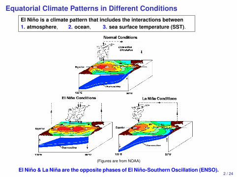
Equatorial Climate Patterns in Different ConditionsEl Niño is a climate pattern that includes the interactions between1. atmosphere, 2. ocean, 3. sea surface temperature (SST).
(Figures are from NOAA)
El Niño & La Niña are the opposite phases of El Niño-Southern Oscillation (ENSO).2 / 24

Remarkable Observational Phenomena of the ENSO
El Niño Southern Oscillation
I Warm phase: El Niño
I Cold phase: La Niña
1980 1985 1990 1995 2000 2005 2010 2015−3
−2
−1
0
1
2
3
Years
Nino 3.4 Index
Super El Nino Super El Nino Super El Nino
Delaying ...
I Eastern Pacific El Niño, including two types of super El Niño: 1) 1982-1983and 1997-1998, 2) 2014-2016. — Lecture 5 & 6.
I A series of moderate El Niño but little La Niña: 1990-1995, 2002-2006— years with central Pacific El Niño (El Niño Modoki) — Lecture 7.
Therefore, ENSO is more than a simple regular oscillator!3 / 24
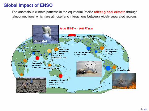
Global Impact of ENSOThe anomalous climate patterns in the equatorial Pacific affect global climate throughteleconnections, which are atmospheric interactions between widely separated regions.
4 / 24
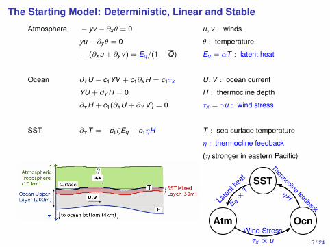
The Starting Model: Deterministic, Linear and Stable
Atmosphere
Ocean
SST
− yv − ∂xθ = 0
yu − ∂yθ = 0
− (∂x u + ∂y v) = Eq/(1− Q)
∂τU − c1YV + c1∂x H = c1τx
YU + ∂Y H = 0
∂τH + c1(∂x U + ∂Y V ) = 0
∂τT = −c1ζEq + c1ηH
u, v : winds
θ : temperature
Eq = αT : latent heat
U,V : ocean current
H : thermocline depth
τx = γu : wind stress
T : sea surface temperature
η : thermocline feedback
(η stronger in eastern Pacific)
SST
Atm OcnLa
tent h
eat
E q∝
TWind Stressτx ∝ u
Thermocline feedback
ηH
5 / 24

The Starting Model: Deterministic, Linear and Stable
Atmosphere
Ocean
SST
− yv − ∂xθ = 0
yu − ∂yθ = 0
− (∂x u + ∂y v) = Eq/(1− Q)
∂τU − c1YV + c1∂x H = c1τx
YU + ∂Y H = 0
∂τH + c1(∂x U + ∂Y V ) = 0
∂τT = −c1ζEq + c1ηH
u, v : winds
θ : temperature
Eq = αT : latent heat
U,V : ocean current
H : thermocline depth
τx = γu : wind stress
T : sea surface temperature
η : thermocline feedback
(η stronger in eastern Pacific)I fundamentally different from the Cane-Zebiak and other nonlinear models that use internal
instability to trigger the ENSO cycles. (plus, emphasis of CZ model: eastern Pacificthermocline.)
I non-dissipative atmosphere consistent with the skeleton model of Madden-Julian Oscillation(Majda and Stechmann 2009, 2011); suitable to describe the dynamics of the Walker circulation
I different meridional axis y and Y due to different Rossby radius in atmosphere and ocean
I allowing a systematic meridional decomposition of the system into the well-known paraboliccylinder functions, keeping the system easily solvable (Majda; 2003)
6 / 24
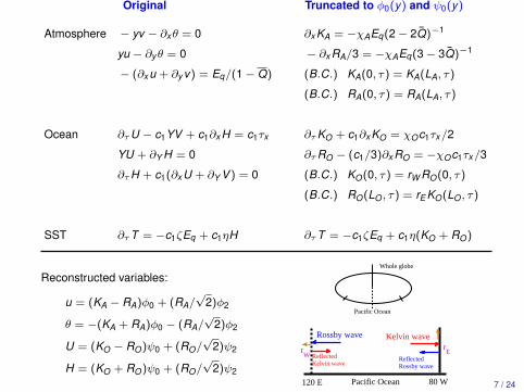
Original Truncated to φ0(y) and ψ0(y)
Atmosphere
Ocean
SST
− yv − ∂xθ = 0
yu − ∂yθ = 0
− (∂x u + ∂y v) = Eq/(1− Q)
∂τU − c1YV + c1∂x H = c1τx
YU + ∂Y H = 0
∂τH + c1(∂x U + ∂Y V ) = 0
∂τT = −c1ζEq + c1ηH
∂x KA = −χAEq(2− 2Q)−1
− ∂x RA/3 = −χAEq(3− 3Q)−1
(B.C.) KA(0, τ) = KA(LA, τ)
(B.C.) RA(0, τ) = RA(LA, τ)
∂τKO + c1∂x KO = χOc1τx/2
∂τRO − (c1/3)∂x RO = −χOc1τx/3
(B.C.) KO(0, τ) = rW RO(0, τ)
(B.C.) RO(LO , τ) = rE KO(LO , τ)
∂τT = −c1ζEq + c1η(KO + RO)
Reconstructed variables:
u = (KA − RA)φ0 + (RA/√
2)φ2
θ = −(KA + RA)φ0 − (RA/√
2)φ2
U = (KO − RO)ψ0 + (RO/√
2)ψ2
H = (KO + RO)ψ0 + (RO/√
2)ψ2
Whole globe
Pacific Ocean
80 W120 E Pacific Ocean
Reflected Rossby wave
ReflectedKelvin wave
rE
Rossby wave Kelvin wave
rW
7 / 24

Yea
r
u
0 5 10 15
1
2
3
4
5
6
−2 0 2
Yea
r
U
0 5 10 15
1
2
3
4
5
6
−0.2 0 0.2
Yea
r
H
0 5 10 15
1
2
3
4
5
6
−20 0 20
Yea
r
T
0 5 10 15
1
2
3
4
5
6
−2 0 2
Atmosphere:
− yv − ∂xθ = 0
yu − ∂yθ = 0
− (∂x u + ∂y v) = Eq/(1 − Q)
Ocean:
∂τ U − c1YV + c1∂x H = c1τx
YU + ∂Y H = 0
∂τ H + c1(∂x U + ∂Y V ) = 0
SST:
∂τ T = −c1ζEq + c1ηH
Linear solution with NA = 64 and NO = 28, where the decay rate is set to be zero forillustration purpose.
8 / 24
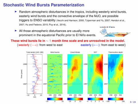
Stochastic Wind Bursts ParameterizationI Random atmospheric disturbances in the tropics, including westerly wind bursts,
easterly wind bursts and the convective envelope of the MJO, are possibletriggers to ENSO variability (Vecchi and Harrison, 2000; Tziperman and Yu, 2007; Hendon et al.,
2007; Hu and Fedorov, 2015; Puy et al., 2016).
I All those atmospheric disturbances are usually moreprominent in the equatorial Pacific prior to El Niño events.
These wind bursts lie in ∼ 1 month time scale and are unresolved in the model.(westerly (−→): from west to east easterly (←−): from east to west
)
−10 0 10
1997
1998
Total winds (140−180)
m/s
Tim
e (y
ear)
150 200 250
1997
1998
Wind bursts
m/s
−20 0 20
150 200 250
1997
1998
Zonal Winds
m/s
−10 0 10
150 200 250
1997
1998
SST
K
−4 −2 0 2 4
150 200 250
1997
1998
Thermocline depth
m
−100 0 100 9 / 24
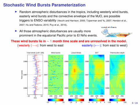
Stochastic Wind Bursts ParameterizationI Random atmospheric disturbances in the tropics, including westerly wind bursts,
easterly wind bursts and the convective envelope of the MJO, are possibletriggers to ENSO variability (Vecchi and Harrison, 2000; Tziperman and Yu, 2007; Hendon et al.,
2007; Hu and Fedorov, 2015; Puy et al., 2016).
I All those atmospheric disturbances are usually moreprominent in the equatorial Pacific prior to El Niño events.
These wind bursts lie in ∼ 1 month time scale and are unresolved in the model.(westerly (−→): from west to east easterly (←−): from east to west
)
−10 0 10
1986
1987
1988
Total winds (140−180)
m/s
Tim
e (y
ear)
150 200 250
1986
1987
1988
Wind bursts
m/s
−20 0 20
150 200 250
1986
1987
1988
Zonal Winds
m/s
−10 0 10
150 200 250
1986
1987
1988
SST
K
−4 −2 0 2 4
150 200 250
1986
1987
1988
Thermocline depth
m
−100 0 100 9 / 24
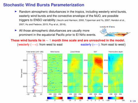
Stochastic Wind Bursts ParameterizationI Random atmospheric disturbances in the tropics, including westerly wind bursts,
easterly wind bursts and the convective envelope of the MJO, are possibletriggers to ENSO variability (Vecchi and Harrison, 2000; Tziperman and Yu, 2007; Hendon et al.,
2007; Hu and Fedorov, 2015; Puy et al., 2016).
I All those atmospheric disturbances are usually moreprominent in the equatorial Pacific prior to El Niño events.
These wind bursts lie in ∼ 1 month time scale and are unresolved in the model.(westerly (−→): from west to east easterly (←−): from east to west
)
−10 0 10
2014
2015
2016
Total winds (140−180)
m/s
Tim
e (y
ear)
150 200 250
2014
2015
2016
Wind bursts
m/s
−20 0 20
150 200 250
2014
2015
2016
Zonal Winds
m/s
−10 0 10
150 200 250
2014
2015
2016
SST
K
−4 −2 0 2 4
150 200 250
2014
2015
2016
Thermocline depth
m
−100 0 100 9 / 24

SST v.s. WWB (from Chen et al, Nature Geoscience, 2015)
contour: SSTblack line: WWB
10 / 24

WWB and EWB in 1998 and 2014 events.(Time series are taken from Hu and Fedorov, PNAS 2016)
(westerly (−→): from west to east easterly (←−): from east to west
)
11 / 24
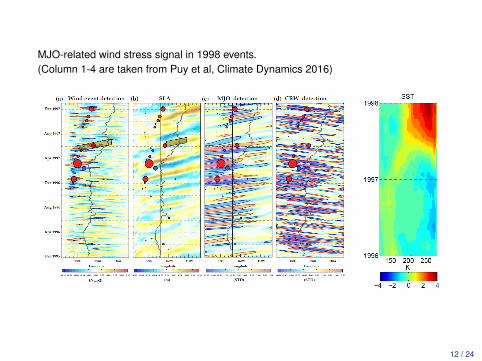
MJO-related wind stress signal in 1998 events.(Column 1-4 are taken from Puy et al, Climate Dynamics 2016)
12 / 24

A summary of the observational facts.
1. Wind bursts, including WWB, EWB and MJO-related winds, are all possibletriggers to ENSO variability.
2. Wind bursts occur in a much faster time scale than the ENSO cycle.
3. Wind bursts are mostly in the western Pacific are their strength is affected by thewarm pool SST (Fedorov et al., 2015; Tziperman and Yu, 2007; Hendon et al., 2007).
Next: Develop a wind burst model that includes all these observational facts.
13 / 24

Stochastic Wind Bursts: in western Pacific depending on warm pool SST
Total wind stress
Wind burst
Evolution
τx = γ(u + up),
up = ap(τ)sp(x)φ0(y)
dap/dτ = −dpap + σp(TW )W (τ),
up : wind bursts,
sp : spatial structure
TW : western Pacific SST
Markov Jump Process: stochastic dependency on warm pool SST
Markov States
States Switch
σp(TW ) =
{σp0 : quiescent
σp1 : active
P(quiescent→ active at t + ∆t) = r01∆t + o(∆t)
P(active→ quiescent at t + ∆t) = r10∆t + o(∆t)
Fundamentally different from Jin et al., 2007 that relies on the eastern Pacific SSTand D. Chen et al., 2015 that requires ad hoc prescription of wind burst thresholds.
14 / 24

Stochastic Wind Bursts: in western Pacific depending on warm pool SST
Total wind stress
Wind burst
Evolution
τx = γ(u + up),
up = ap(τ)sp(x)φ0(y)
dap/dτ = −dpap + σp(TW )W (τ),
up : wind bursts,
sp : spatial structure
TW : western Pacific SST
Markov Jump Process: stochastic dependency on warm pool SST
Markov States
States Switch
σp(TW ) =
{σp0 : quiescent
σp1 : active
P(quiescent→ active at t + ∆t) = r01∆t + o(∆t)
P(active→ quiescent at t + ∆t) = r10∆t + o(∆t)
Fundamentally different from Jin et al., 2007 that relies on the eastern Pacific SSTand D. Chen et al., 2015 that requires ad hoc prescription of wind burst thresholds. 14 / 24
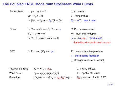
The Coupled ENSO Model with Stochastic Wind Bursts
Atmosphere
Ocean
SST
− yv − ∂xθ = 0
yu − ∂yθ = 0
− (∂x u + ∂y v) = Eq/(1− Q)
∂τU − c1YV + c1∂x H = c1τx
YU + ∂Y H = 0
∂τH + c1(∂x U + ∂Y V ) = 0
∂τT = −c1ζEq + c1ηH
u, v : winds
θ : temperature
Eq = αT : latent heat
U,V : ocean current
H : thermocline depth
τx = γ(u+up) : wind stress
(including stochastic wind bursts)
T : sea surface temperature
η : thermocline feedback
(η stronger in eastern Pacific)
Total wind stress
Wind burst
Evolution
τx = γ(u + up),
up = ap(τ)sp(x)φ0(y)
dap/dτ = −dpap + σp(TW )W (τ),
up : wind bursts,
sp : spatial structure
TW : western Pacific SST
15 / 24

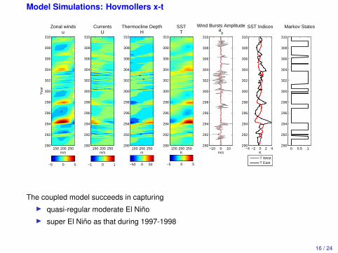
Model Simulations: Hovmollers x-t
m/s
Y
ear
Zonal windsu
150 200 250100
102
104
106
108
110
112
114
116
118
120
−5 0 5
m/s
CurrentsU
150 200 250100
102
104
106
108
110
112
114
116
118
120
−1 0 1
m
Thermocline DepthH
150 200 250100
102
104
106
108
110
112
114
116
118
120
−50 0 50
K
SSTT
150 200 250100
102
104
106
108
110
112
114
116
118
120
−5 0 5
−10 0 10100
102
104
106
108
110
112
114
116
118
120
m/s
Wind Bursts Amplitudea
p
−4 −2 0 2 4100
102
104
106
108
110
112
114
116
118
120
K
SST Indices
T West
T East
0 0.5 1100
102
104
106
108
110
112
114
116
118
120
Markov States
The coupled model succeeds in capturingI quasi-regular moderate El Niño
I super El Niño as that during 1997-1998I super El Niño as that during 2014-2016
16 / 24
Model Simulations: Hovmollers x-t
Yea
r
Zonal windsu
m/s150 200 250
290
292
294
296
298
300
302
304
306
308
310
−5 0 5
0 0.5 1290
292
294
296
298
300
302
304
306
308
310
Markov States
CurrentsU
m/s150 200 250
290
292
294
296
298
300
302
304
306
308
310
−1 0 1
Thermocline DepthH
m150 200 250
290
292
294
296
298
300
302
304
306
308
310
−50 0 50
SSTT
K150 200 250
290
292
294
296
298
300
302
304
306
308
310
−5 0 5
−10 0 10290
292
294
296
298
300
302
304
306
308
310
Wind Bursts Amplitudea
p
m/s−4 −2 0 2 4
290
292
294
296
298
300
302
304
306
308
310
SST Indices
K
T WestT East
The coupled model succeeds in capturingI quasi-regular moderate El NiñoI super El Niño as that during 1997-1998
I super El Niño as that during 2014-2016
16 / 24
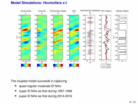
Model Simulations: Hovmollers x-t
Yea
r
m/s
Zonal windsu
150 200 250140
142
144
146
148
150
152
154
156
158
160
−5 0 5
m/s
CurrentsU
150 200 250140
142
144
146
148
150
152
154
156
158
160
−1 0 1
Thermocline DepthH
m150 200 250
140
142
144
146
148
150
152
154
156
158
160
−50 0 50
K
SSTT
150 200 250140
142
144
146
148
150
152
154
156
158
160
−5 0 5
−10 0 10140
142
144
146
148
150
152
154
156
158
160
m/s
Wind Bursts Amplitudea
p
−4 −2 0 2 4140
142
144
146
148
150
152
154
156
158
160
K
SST Indices
T WestT East
0 0.5 1140
142
144
146
148
150
152
154
156
158
160
Yea
r
Markov States
The coupled model succeeds in capturingI quasi-regular moderate El NiñoI super El Niño as that during 1997-1998I super El Niño as that during 2014-2016
16 / 24
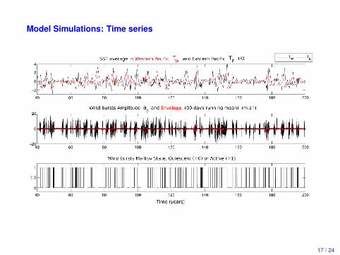
Model Simulations: Time series
17 / 24

Model Simulations: PDF and Power SpectrumModerate and Extreme El Niño events in the eastern Pacific, frequency ≈ 2-7 years.
The fat-tailed non-Gaussian PDF in the model is due to the state-dependentnoise in the stochastic wind bursts.
18 / 24

Model Simulations: PDF and Power SpectrumModerate and Extreme El Niño events in the eastern Pacific, frequency ≈ 2-7 years.
The fat-tailed non-Gaussian PDF in the model is due to the state-dependentnoise in the stochastic wind bursts. 18 / 24

Mechanism of the overall ENSO formation
19 / 24

Mechanism of 1997-1998 El Niño
Observations1997-1998
Model SimulationMimicking 1997-1998
20 / 24

Mechanism of 2014-2016 El Niño
Observations2014-2016
Model SimulationMimicking 2014-2016
21 / 24
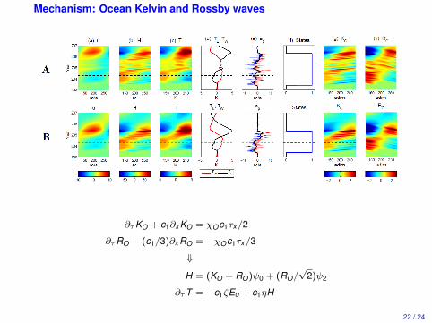
Mechanism: Ocean Kelvin and Rossby waves
∂τKO + c1∂x KO = χOc1τx/2
∂τRO − (c1/3)∂x RO = −χOc1τx/3
⇓
H = (KO + RO)ψ0 + (RO/√
2)ψ2
∂τT = −c1ζEq + c1ηH
22 / 24
Summary
A simple modeling framework is developed for the ENSO.
1. The starting model is a coupled ocean-atmosphere model that is deterministic,linear and stable.
2. A stochastic parameterization of the wind bursts including both westerly andeasterly winds is coupled to the simple ocean-atmosphere system.
3. The coupled model succeeds in simulating traditional El Niño and capturing theobservational record in the eastern Pacific.
4. The coupled model is able to distinguish the two types of super El Niño. (Moredetails will be discussed in Lecture 6 by Sulian Thual)
5. With more physics in the model (such as nonlinear advection and mean tradewind anomaly), the simple modeling framework allows the study of central PacificEl Niño and therefore the El Niño diversity (Lecture 7, 8, 9).
23 / 24
Next week by Sulian Thual:Mechanisms of the 2014-2016 delayed super El Niño capturing by simple dynamicalmodels.
Thank you
24 / 24