The P/B-ROE Model Revisited
Jarrod Wilcox
Wilcox Investment Inc
&
Thomas Philips
Paradigm Asset Management

2
Agenda
§ Characterizing a good equity model: Its virtues and uses
§ Static vs. dynamic models
§ The P/B-ROE model: Closed form & approximate solutions
§ Cross-sectional explanation using the P/B-ROE model
§ Cross-sectional prediction using the P/B-ROE model
§ Time-series explanation using the P/B-ROE model
§ Time-series prediction using the P/B-ROE model
3
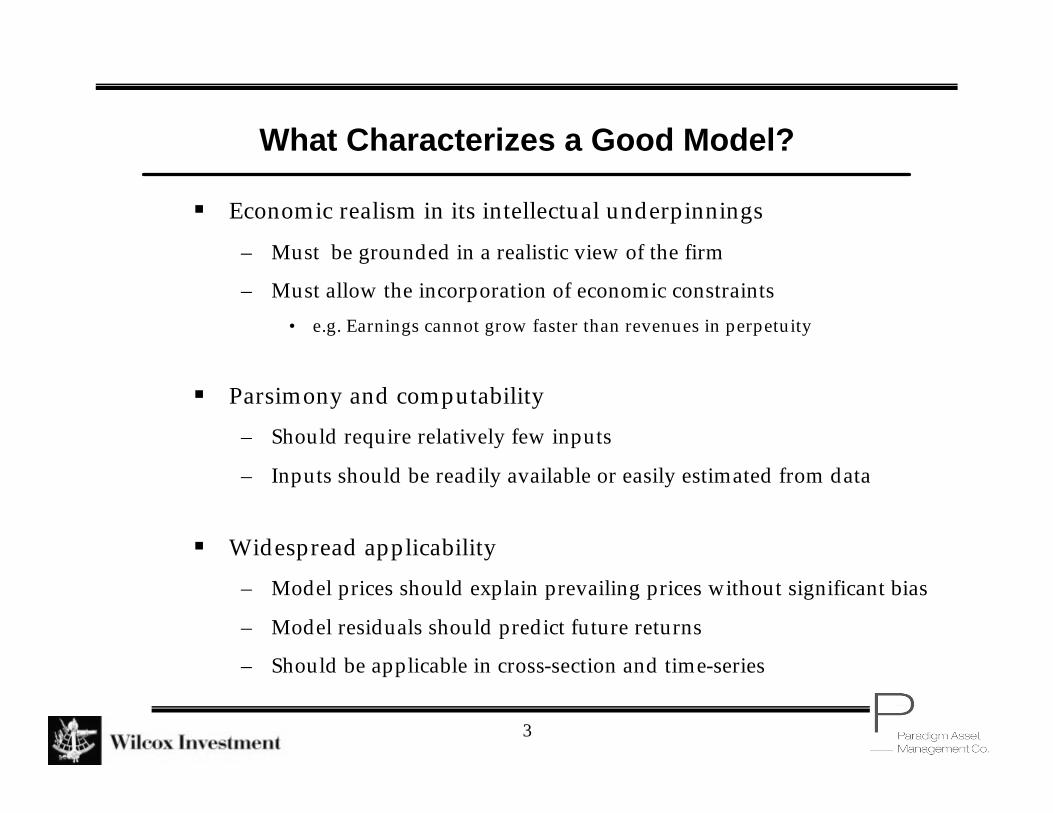
What Characterizes a Good Model?
§ Economic realism in its intellectual underpinnings
– Must be grounded in a realistic view of the firm
– Must allow the incorporation of economic constraints• e.g. Earnings cannot grow faster than revenues in perpetuity
§ Parsimony and computability– Should require relatively few inputs
– Inputs should be readily available or easily estimated from data
§ Widespread applicability– Model prices should explain prevailing prices without significant bias
– Model residuals should predict future returns
– Should be applicable in cross-section and time-series

4
Who Might Use a Good Model?
§ Corporate officers
– If the model can guide them on how best to increase firm value
§ Fundamental analysts– If the model can help them better evaluate a firm and its management
§ Investment bankers and buyers and sellers of companies– If the model can generate unbiased valuations
§ Investors– If the model’s residuals are predictive of future returns

5
Models in Widespread Use Today
§ Dividend Discount Model (J.B. Williams, 1938):
– Intellectual root of almost all models in use today
§ Gordon Growth model (1962):
– Free cash flows grow at a constant rate in perpetuity
§ Edward-Bell-Ohlson Equation (1961):
– Apply clean surplus relationship to DDM and rearrange terms
§ Various multi-stage versions of the DDM
– 3 stages model growth, steady state and decline
gkP
−= 1FlowCash Free
∑∞
=
−
+×−
+=1
10 )1(
])[(
ii
ii
kBkrE
BP
∑∞
= +=
10 )1(
][
iii
kFCFE
P
6
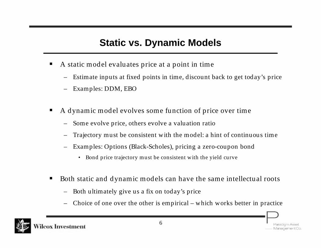
Static vs. Dynamic Models
§ A static model evaluates price at a point in time
– Estimate inputs at fixed points in time, discount back to get today’s price
– Examples: DDM, EBO
§ A dynamic model evolves some function of price over time
– Some evolve price, others evolve a valuation ratio
– Trajectory must be consistent with the model: a hint of continuous time
– Examples: Options (Black-Scholes), pricing a zero-coupon bond• Bond price trajectory must be consistent with the yield curve
§ Both static and dynamic models can have the same intellectual roots
– Both ultimately give us a fix on today’s price
– Choice of one over the other is empirical – which works better in practice

7
A Brief History of Dynamic Models
§ Jarrod Wilcox (FAJ 1984): P/B-ROE model.
– Two stage growth model ,with first phase ending at time T.
– Determine the trajectory of P/B subject to the constraint P/BT=1
– Obtain today’s P/B from trajectory & terminal condition:
§ Tony Estep (FAJ 1985, JPM 2003): T (or Total Return) model– Follows P/B-ROE logic, but arbitrarily sets time horizon to 20 years
– Derives and tests a holding period return:
§ Marty Leibowitz (FAJ 2000): P/E Forwards And Their Orbits– P/E must evolve along certain paths (orbits) determined by k
– Has implications for current P/E
– Theoretical, no tests of explanatory or predictive power
( ) TkrBP )(/ln −=
( )gBPBP
BPgr
gT +∆
+
−
+= 1//
/
8
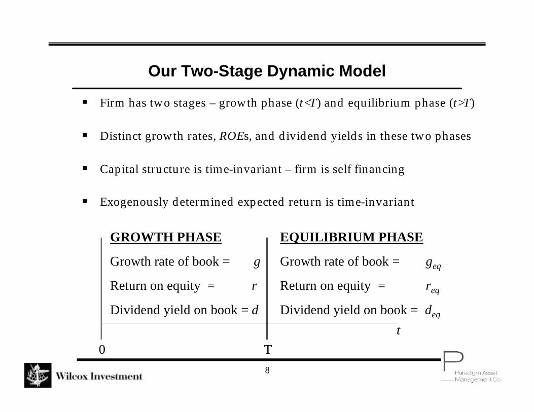
Our Two-Stage Dynamic Model
§ Firm has two stages – growth phase (t<T) and equilibrium phase (t>T)
§ Distinct growth rates, ROEs, and dividend yields in these two phases
§ Capital structure is time-invariant – firm is self financing
§ Exogenously determined expected return is time-invariant
tT
GROWTH PHASE
Growth rate of book = g
Return on equity = r
Dividend yield on book = d
EQUILIBRIUM PHASE
Growth rate of book = geq
Return on equity = req
Dividend yield on book = deq
0

9
Economic Intuition and More Notation
§ We evolve = Price-to-Book ratio at time t
§ Dt = Cumulative dividend process at time t
§ r = Instantaneous ROE = growth + dividend yield on book = g+d
§ k = Required shareholder return, assumed constant for all t>0.
tBP /
t0 T
BP /
Trajectory of P/B in the growth
phase must be consistent with k
TBP /
Growth Phase Equilibrium

10
Exact Solution - I
§ Total Return = Price Return + Dividend yield
§ If all parameters are time invariant:
§ (1)
§ In addition, we always have (2)
§ Differentiate (2) w.r.t. time and divide by price to get
§ (3)
tD
PtP
PPt
DtP
k t
t
t
tt
tt
∂∂
+∂∂
=∂∂
+∂∂
==11
Return Total
ttt BPBP /×=
tB
BtBP
BPtP
Pt
t
t
t
t
t ∂∂
+∂
∂=
∂∂ 1/
/11
11
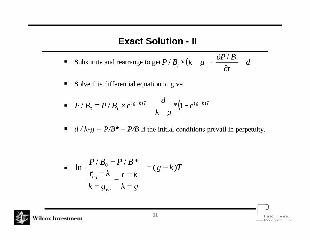
Exact Solution - II
§ Substitute and rearrange to get
§ Solve this differential equation to give
§
§ d / k-g = P/B* = P/B if the initial conditions prevail in perpetuity.
§
( ) dtBP
gkBP tt +
∂∂
=−×/
/
( )TkgTkgT e
gkd
eBPBP )()(0 1*// −− −
−+×=
Tkg
gkkr
gkkr
BPBP
eq
eq
)(*//
ln 0 −=
−−
−−
−−

12
Approximation: All Profits Are Reinvested In Growth Phase
§ Then d=0, r = g, and TkrT eBPBP )(
0 // −×=
.51
24
816
Pric
e/B
ook
-10% 0% 10% 20% 30% 40%Expected Return on Equity
d = 0% d = 6%
Impact of Dividends on P/B-ROE Model

13
Approximate Solution: The P/B-ROE Model
§ Take natural log on both sides to get
§ In Jarrod’s 1984 paper, , but this is unrealistic today
§ The P/B-ROE model can be estimated from data via OLS regression
– Can proxy r with ROE, as profitability tends to be stable and mean-reverting.
– Can use analysts’ estimates to further enhance our estimate of r.
– Hard to extract information from constant, so focus on estimating T
§ Run cross-sectional (U.S. stocks) and time-series (S&P 500) regressions
§ Determine fit of regression (cross-sectional & time-series explanation)
§ Use residuals to forecast returns (cross-sectional and time-series prediction)
( ) ( ) ( )[ ] rTkTBPTkrBPBP TT +−=−+= /ln)(/ln/ln 0
1/ =TBP
14
Cross Sectional Explanation
§ How much should CEO’s expect stock price to increase for each 1%
in additional ROE?
§ Sample: ValueLine Datafile 1988-2002, companies with fiscal year-ends in December, positive book value, and ROE between -10% and +40%. Over 20,000 observations.
§ Run panel regression of ln(P/B) against ROE
§ Slope of regression line depends on past volatility of ROE.
§ We interpret this slope as a measure of the investment horizon T.

15
Long-term Panel Results
§ The pooled slope within each year of the 1988-2002 period is 3.66
years. For very stable companies it rises to about 9 years.
§ A stable ROE allows projecting recent values further into the future.
§ Independent of risk premium, ROE stability can either help or hurt through its impact on investment horizon T.
6.475.003.872.37T (years)
4
Lowest 5-year
ROE Volatility
321
Highest 5-year
ROE Volatility
QUARTILES:

16
Example Drawn From 1988-2002 Averages
§ Consider a stock with ROE = 15%, and in the 4th quartile of
ROE stability (5-year standard deviation of ROE < 2.5%).
§ Regression slope (our estimate of T): 6.47 years
§ Question: Other things equal, how much higher would its
price be if its ROE were 20%?
§ Answer: Its stock price would have been 38% higher, not
counting any increase in book value B.
17
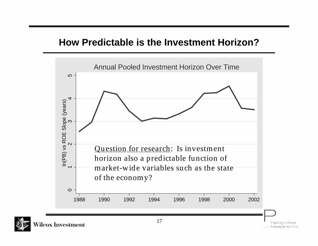
How Predictable is the Investment Horizon?
01
23
45
ln(P
B)
vs R
OE
Slo
pe (
year
s)
1988 1990 1992 1994 1996 1998 2000 2002
Annual Pooled Investment Horizon Over Time
Question for research: Is investment horizon also a predictable function of market-wide variables such as the state of the economy?
18
Interpretation of Explanatory Models
§ Across the full sample, R2 = 26%. It approaches 50% for more stable
companies. R2 biased upward by random B, and downward by pooling across company types and time.
§ Statistical models involving valuation ratios should be translated into standard errors in log price to judge their merits.
§ Apparent degrees of freedom are inflated because of clustering of observations by industry. However, they are still very large.
§ Though useful in practice, interpreting slope as T may also incorporate an errors-in-variables bias from using ROE as a proxy for r.
§ In an efficient market, even a very good explanatory model for prices may not forecast returns.
19
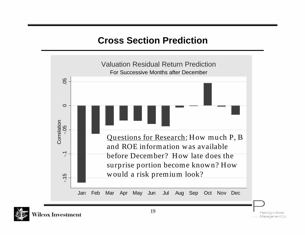
Cross Section Prediction
-.15
-.1-.0
50
.05
Cor
rela
tion
Jan Feb Mar Apr May Jun Jul Aug Sep Oct Nov Dec
For Successive Months after DecemberValuation Residual Return Prediction
Questions for Research: How much P, B and ROE information was available before December? How late does the surprise portion become known? How would a risk premium look?

20
Regression Coefficients1988-2002 December Residuals vs. Future Returns.
0.10%-4.5-.011July – September
0.38%-8.7-.022April – June
2.22%-21.2-.055January – March
Adjusted R2t-statisticOLS CoefficientPeriod

21
Hypothetical Cross-sectional Return Forecast Success
-12
-8-4
04
t-Sta
tistic
1989 1991 1993 1995 1997 1999 2001 2003
Ability to Forecast April-June Return Differences
Does P/B-ROE capture periods of reversion to fundamentals?

22
Cross-Sectional Summary
§ P/B-ROE gives both the company and the market a helpful tool
to calibrate the impact of financial plans on shareholder value.
§ Model residuals have predictive power, and are likely to be a
useful addition to the investor’s toolbox, even before
disaggregating by time and industry.
§ P/B-ROE allows a value approach for growth stocks, and is less
biased against high quality growth than are traditional ratios
like P/E, P/B, P/S, and P/CF.
23
Why Improve Explanatory Models for the S&P 500?
§ To increase market stability by showing relevance of
fundamentals and identifying bubbles.
§ To better show forecasters the impact of changes in
fundamentals.
§ If the market departs from forecastable fundamentals, to
help forecast returns using valuation residuals.
24
Relevant Structure
§ If ln(P/B) = ln(P/BT) + T * (r - k), comparisons of E/P to interest rates (so-called Fed Model) are badly mis-specified.
• See also “Fight The Fed Model” by Cliff Asness (JPM, 2003)
§ Changing monetary inflation complicates this picture further
§ Higher rates of inflation both:
• Raise nominal k
• Lower replacement cost profitability and thus r from reported ROE.
§ We therefore model ln(P/B) as a linear function of ROE, inflation, and real interest rates.

25
Model Inputs (updated)
0.0
5.1
.15
.2.2
5A
nnua
l Rat
e
1976 1980 1984 1988 1992 1996 2000 2004gdate
ROE Real_InterestInflation
P/B-ROE S&P500 Model Inputs
§ ROE: S&P 500’s S E/ S P
§ Inflation: 12 Month CPI % Change
§ Real Interest: Moody’s AAA Yield – 12 Month CPI % Chg.

26
Full Sample S&P500 Index Model
§ Because of omitted variables, the model errors are highly
autocorrelated. R-squared of the fit is highly inflated.
§ ln(P/B)S&P500 = 1.1 + 6.3 * ROE – 15.9 * Inflation – 8.0 * Real Interest
§ When appraising the model’s hypothetical use as an
prediction tool, it is important to avoid look-ahead bias.
– Use expanding window regression after 5-year warm-up period.
27
What Does P/B-ROE Tell US? (updated)
12
34
56
Pric
e-to
-Boo
k R
atio
1976 1980 1984 1988 1992 1996 2000 2004
Actual No_LookAhead
S&P500 Actual P/B and Expanding Window Explanation

28
Using A Regression Model With Unstable Missing Variables
§ We know that the regression model is not fully satisfied
– The process is not stable
§ Residuals are highly autocorrelated due to missing variables
– Changes in risk preference?
– Changing ROE cross-sectional dispersion?
– Changing taxation?
§ Consequently, we do not assume that correlation automatically
translates into a successful investment decision,
§ But...

29
Correlation: P/B-ROE Residuals vs. 1 month S&P 500 Returns
-0.2
0-0
.10
0.00
0.10
0.20
-0.2
0-0
.10
0.00
0.10
0.20
-15 -10 -5 0 5 10 15Lag
Do P/B-ROE Residuals Predict S&P 500 Returns?
30
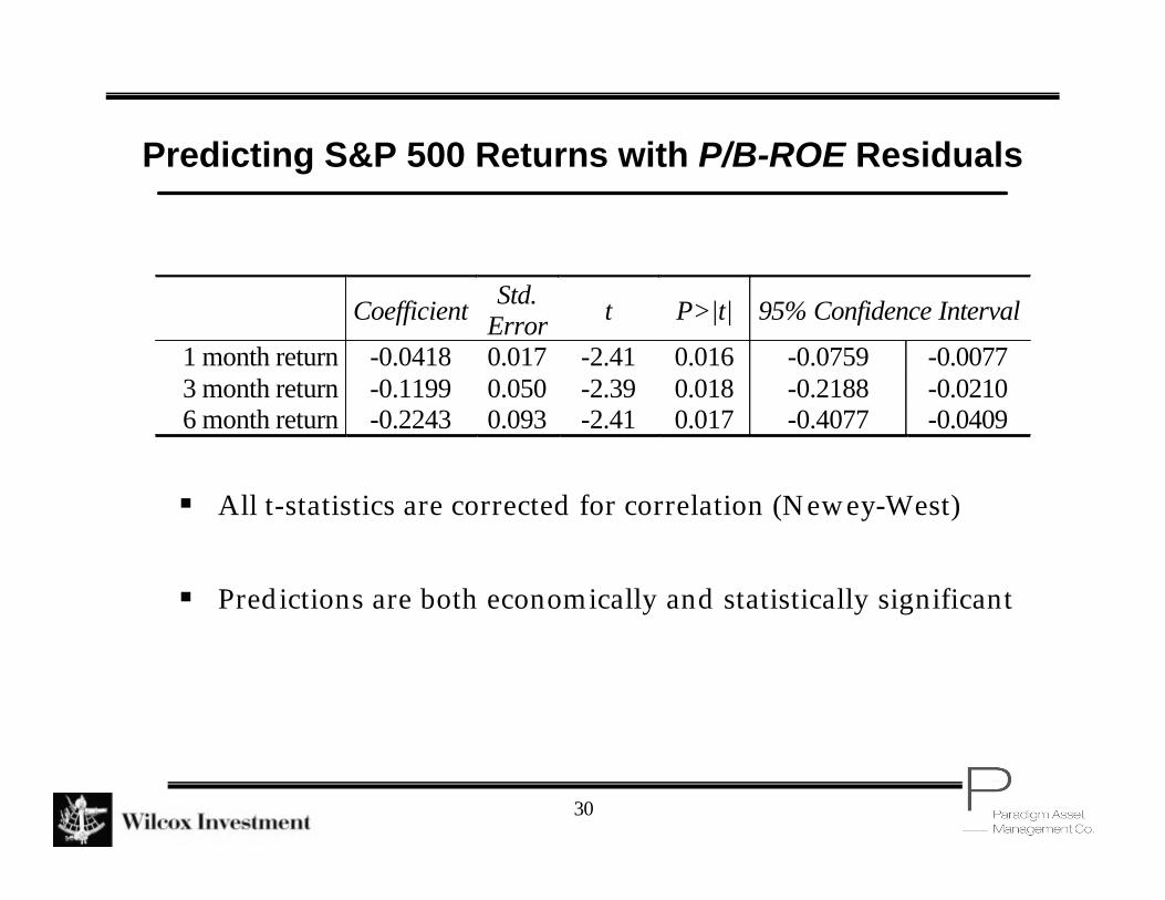
Predicting S&P 500 Returns with P/B-ROE Residuals
Coefficient Std. Error t P>|t| 95% Confidence Interval
1 month return -0.0418 0.017 -2.41 0.016 -0.0759 -0.0077 3 month return -0.1199 0.050 -2.39 0.018 -0.2188 -0.0210 6 month return -0.2243 0.093 -2.41 0.017 -0.4077 -0.0409
§ All t-statistics are corrected for correlation (Newey-West)
§ Predictions are both economically and statistically significant
31
P/B-ROE Time-Series Confirms Cross-section
§ Implied investment horizon T against ROE for the S&P500 is similar
to that found in cross-section for stocks in the most stable quartile.
§ When supplemented by allowance for time-varying inflation and
interest rates, P/B-ROE:– Identifies key fundamentals controlling valuation, useful for planning
– Is structurally different from E/P versus interest rate comparisons• See “Fight The Fed Model”, Cliff Asness (JPM 2003)
– Provides useful short-term coincident explanation
§ In addition, its residuals also show potential for use as an ingredient
in tactical asset allocation (TAA)
32
Summary
§ P/B-ROE is both simple and effective for a wide range of problems
§ Some investment managers have used P/B-ROE for many years as
an additional valuation factor...
§ But it not used as widely as it could be:– By CEO’s, CFO’s and analysts
– And for identifying undervalued growth stocks
– And to better identify bubbles
– And as an ingredient in tactical asset allocation
§ And generally to enhance the importance of fundamentals as opposed to momentum in investing and pricing.