Optimal Configuration of a
Planet-Finding Mission Consisting of a
Telescope and a Constellation of
Occulters
Egemen Kolemen
A Dissertation
Presented to the Faculty
of Princeton University
in Candidacy for the Degree
of Doctor of Philosophy
Recommended for Acceptance
by the Department of
Mechanical and Aerospace Engineering
Adviser: N. Jeremy Kasdin
SEPTEMBER 2008

c© Copyright by Egemen Kolemen, 2008.
All Rights Reserved
Abstract
Occulter-based telescopy offers a promising new terrestrial planet-finding method-
ology that involves the formation flying of a conventional space telescope with a
large external occulter, which will block the light of a star and allow imaging of
its dim, close-by planetary companion. Recent advances in shaped-pupil technology
have enabled the design of occulters that have superior diffraction performance and
that can be manufactured easily. This approach is attractive because it eliminates
the precision-optical requirements of the alternative coronagraphic or interferometric
approaches. However, it introduces new scientific challenges in the area of precise
dynamics and control, which is the topic of this dissertation.
Due to the large distances between satellites, realignment is fuel intensive, which
increases the mission cost and reduces its lifetime. In order to overcome this problem,
this dissertation focuses on the trajectory design of the mask satellite and conducts
an optimization study to select the order and timing of imaging sessions.
The optimal configuration of satellite formations consisting of a telescope and
multiple occulters around Sun-Earth L2 Halo orbits is studied first. Focusing on the
Quasi-Halo orbits, which are of interest for fuel-free occulter placement, the phase
space around L2 is examined. The periodic orbits of interest around L2 are numeri-
cally computed and their stability properties analyzed.
Quasi-Halos are good candidates for occulter placement, as they are fuel-free orbits
and have large sky coverage with respect to the Halo orbit, where the telescope is
placed. With the aim of identifying these orbits, a new fully numerical method that
employs multiple Poincare sections to find quasi-periodic orbits is developed. This
methodology has the advantage of very fast execution times and robust behavior
near chaotic regions that leads to full convergence. Its numerical implementations for
Lissajous and Quasi-Halo orbits are explained. These results are then extended from
the simplified three body model to find the orbits in the real solar system that have
iii
the same characteristics.
Trajectory optimization of the occulter motion between imaging sessions of differ-
ent stars is performed using a range of different criteria and methods. This enables
the transformation of the global optimization problem into a Time-Dependent Trav-
eling Salesman Problem (TSP). The TSP is solved first for a formation consisting of
a telescope and a single occulter. Then, with the insight from the dynamical analysis,
multiple-occulter formations are analyzed and the global optimization is performed
for the multiple-occulter case.
For a concrete understanding of the feasibility of the mission, the performance of
an example spacecraft, SMART-1, is analyzed. The mission is shown to be feasible
with the current technology.
iv
Acknowledgements
It has been a great pleasure to work on this project in the Department of Mechanical
and Aerospace Engineering at Princeton University. I owe a great debt of gratitude
to my advisor, Jeremy Kasdin. Jeremy has been a truly inspiring mentor, allowing
me significant freedom in my choice of research topics, even in my first year, and
always encouraging me to explore side research interests. I deeply appreciate his
advice, support, and encouragement over the years. Jeremy has the true spirit of a
researcher; a quality, which I hope I will be able to emulate.
I would also like to acknowledge several other individuals who have influenced and
supported me in different ways.
Pini Gurfil was very kind to host me at Technion, where, with his support, I
developed the most important ideas of this thesis. I have worked well with him on
several publications, and I look forward to continue to collaborate with him.
Jerry Marsden welcomed me as a visiting scholar at Caltech, where I had the
opportunity to benefit from an amazing creative atmosphere.
Bob Vanderbei has shared his love for astronomy with me and sparked my interest
in celestial mechanics. I enjoyed our collaboration on the rings of Saturn and I hope
to work with him again on other topics in the future. Bob also very kindly agreed to
read my thesis.
Dave Gates has been a wonderful boss at PPPL, where, as a postdoctoral fellow,
I will continue my research on plasma control.
Clancy Rowley has been there from the first day and has helped shape my Prince-
ton experience. I look forward to working with both Clancy and Dave next year.
Rob Stengel very kindly agreed to be my reader. He sent me extensive and much
appreciated comments during what should have been his holiday. For this, I am very
grateful.
Naomi Leonard taught me the foundations of controls and dynamics and has been
v

very supportive over the years.
As my examiner, Dick Miles asked me very interesting and challenging questions.
The members of the TPF group at Princeton have been great colleagues and
friends. I will miss them all.
Finally, I would like to thank Jessica O’Leary for holding the MAE Department
together.
To each of the above, I extend my deepest appreciation.
I dedicate this dissertation to Barbara Buckinx, my wonderful girlfriend, best
friend, and confidante, without whom this work wouldn’t have been possible, and to
my loving family, my parents Nilgun and Osman and my sister Aysuda, who never
cease to support me, and who are proud of me from a distance.
This thesis carries the number 3185-T in the records of the Department of Me-
chanical and Aerospace Engineering.
vi

Barbara, Nilgun, Osman ve Aysuda’ya
vii
Contents
Abstract . . . . . . . . . . . . . . . . . . . . . . . . . . . . . . . . . . . . . iii
Acknowledgements . . . . . . . . . . . . . . . . . . . . . . . . . . . . . . . v
1 Extrasolar Planet Imaging and Occulter-Based Telescopy 1
1.1 Finding Extrasolar Life . . . . . . . . . . . . . . . . . . . . . . . . . . 3
1.1.1 Life-Sustaining Planets . . . . . . . . . . . . . . . . . . . . . . 3
1.1.2 Signs of Life . . . . . . . . . . . . . . . . . . . . . . . . . . . . 3
1.1.3 Challenges associated with imaging planets in the habitable zone 5
1.2 External Occulter for Exoplanet Imaging . . . . . . . . . . . . . . . . 8
1.3 Dissertation Outline . . . . . . . . . . . . . . . . . . . . . . . . . . . 10
2 Dynamical Analysis of the L2 Region 13
2.1 Circularly Restricted Three Body Problem - Equations of Motion . . 15
2.2 Equilibrium Points . . . . . . . . . . . . . . . . . . . . . . . . . . . . 19
2.3 Series Expansion around L2 . . . . . . . . . . . . . . . . . . . . . . . 21
2.3.1 Translation of L2 to the origin, and rescaling . . . . . . . . . 21
2.3.2 Series Expansion of the Equations . . . . . . . . . . . . . . . . 23
2.4 Analysis of the Linear Part around L2 . . . . . . . . . . . . . . . . . 24
2.5 High-Order Analysis (The Lindstedt-Poincare Procedure and Halo Or-
bits) . . . . . . . . . . . . . . . . . . . . . . . . . . . . . . . . . . . . 27
2.6 Reduction to Center Manifold . . . . . . . . . . . . . . . . . . . . . . 31
viii
2.6.1 Transformation into complex normal form . . . . . . . . . . . 31
2.6.2 The Procedure Explained . . . . . . . . . . . . . . . . . . . . 34
2.6.3 Implementation of the Lie Series Method . . . . . . . . . . . . 35
3 Periodic Orbits of Interest around L2: Numerical Methods 38
3.1 Numerical Tools for Periodic Libration Orbits around L2 . . . . . . . 39
3.1.1 Collocation as a Numerical Tool to Find Periodic Orbits . . . 40
3.1.2 Stability Analysis of Periodic Orbits . . . . . . . . . . . . . . 43
3.2 Application to the Periodic Orbits of the CRTBP Around L2 . . . . . 46
3.2.1 Horizontal Lyapunov Orbits . . . . . . . . . . . . . . . . . . . 49
3.2.2 Vertical Lyapunov Orbits . . . . . . . . . . . . . . . . . . . . 52
3.2.3 Halo Orbits . . . . . . . . . . . . . . . . . . . . . . . . . . . 55
4 Multiple Poincare Sections Method for Finding the Quasi-Halo and
Lissajous Orbits 58
4.1 Procedure . . . . . . . . . . . . . . . . . . . . . . . . . . . . . . . . . 60
4.1.1 Finding Invariant Tori via a Single Poincare Section . . . . . . 60
4.1.2 Extension to Multiple Poincare Sections . . . . . . . . . . . . 65
4.1.3 Different Implementations . . . . . . . . . . . . . . . . . . . . 67
4.1.4 Continuation Procedure . . . . . . . . . . . . . . . . . . . . . 69
4.2 Numerical Application for the Quasi-Periodic Orbits Around the L2
Region of the CRTBP . . . . . . . . . . . . . . . . . . . . . . . . . . 70
4.2.1 Initial estimate for Q . . . . . . . . . . . . . . . . . . . . . . . 72
4.2.2 Choosing the Poincare Section Surfaces . . . . . . . . . . . . . 74
4.2.3 Choosing θ and computing its derivativedθXτ
dXτ. . . . . . . . . 75
4.2.4 Computing Aθ and DA . . . . . . . . . . . . . . . . . . . . . . 78
4.2.5 Augmenting the error vector F and its derivative DF . . . . . 80
4.2.6 Numerical Integration of the Orbits . . . . . . . . . . . . . . . 82
ix

4.2.7 Numerical computation of the Poincare map . . . . . . . . . . 83
4.2.8 Numerical Computation of the Derivative of the Poincare map 84
4.2.9 Continuation . . . . . . . . . . . . . . . . . . . . . . . . . . . 85
4.3 Results . . . . . . . . . . . . . . . . . . . . . . . . . . . . . . . . . . . 87
4.3.1 Lissajous Orbits . . . . . . . . . . . . . . . . . . . . . . . . . . 88
4.3.2 Quasi-Halo Orbits . . . . . . . . . . . . . . . . . . . . . . . . 90
4.3.3 Complete Periodic Family around L2 . . . . . . . . . . . . . . 91
4.3.4 Comparison of the Results with the Literature . . . . . . . . . 92
4.4 Extension of the CRTBP Results to the Full Ephemeris Model . . . . 93
5 Finding the Optimal Trajectories 101
5.1 Different Optimal Control Approaches . . . . . . . . . . . . . . . . . 102
5.1.1 The Euler-Lagrange Formulation of the Optimal Control Prob-
lem (Indirect Method) . . . . . . . . . . . . . . . . . . . . . . 104
5.1.2 The Sequential Quadratic Programming Formulation of the Op-
timal Control Problem (Direct Method) . . . . . . . . . . . . 106
5.2 Unconstrained Minimum Energy Optimization . . . . . . . . . . . . . 109
5.3 Constrained Minimum Energy Optimization . . . . . . . . . . . . . . 114
5.4 Free-End Condition Optimization . . . . . . . . . . . . . . . . . . . . 120
5.5 Minimum-Time Optimization . . . . . . . . . . . . . . . . . . . . . . 123
5.6 The Minimum-Fuel Optimization . . . . . . . . . . . . . . . . . . . . 129
5.7 Impulsive Thrust: Minimum-Fuel Optimization . . . . . . . . . . . . 134
5.8 Conclusion . . . . . . . . . . . . . . . . . . . . . . . . . . . . . . . . . 136
6 Global Optimization of the Mission: The Traveling Salesman Prob-
lem 138
6.1 Realignment Cost Analysis . . . . . . . . . . . . . . . . . . . . . . . . 140
6.2 Defining the Global Optimization Problem . . . . . . . . . . . . . . . 141
x

6.3 The Classical Traveling Salesman Problem . . . . . . . . . . . . . . . 143
6.4 Mathematical Formulation of the Global Optimization Problem . . . 146
6.4.1 Cost function . . . . . . . . . . . . . . . . . . . . . . . . . . . 146
6.4.2 Including the revisits into the formulation . . . . . . . . . . . 147
6.4.3 Full Formulation . . . . . . . . . . . . . . . . . . . . . . . . . 149
6.5 Numerical Methods Employed for Solving the Global Optimization
Problem . . . . . . . . . . . . . . . . . . . . . . . . . . . . . . . . . . 150
6.5.1 Simulated annealing . . . . . . . . . . . . . . . . . . . . . . . 151
6.5.2 Branching for time-optimal case . . . . . . . . . . . . . . . . . 155
6.5.3 Results . . . . . . . . . . . . . . . . . . . . . . . . . . . . . . . 156
6.6 Performance of SMART-1 as an Occulter . . . . . . . . . . . . . . . . 159
6.7 Multiple Occulters . . . . . . . . . . . . . . . . . . . . . . . . . . . . 162
6.7.1 Multiple Occulters on Quasi-Halo Orbits . . . . . . . . . . . . 163
6.7.2 Global Optimization with Constraints . . . . . . . . . . . . . 164
7 Conclusion 170
xi
Chapter 1
Extrasolar Planet Imaging and
Occulter-Based Telescopy
1
Studying terrestrial and giant planets outside the solar system is one of the primary
goals of NASA’s Origins Program. It is likely that the next decade will see NASA
launch the first in a series of missions dubbed Terrestrial Planet Finders (TPF) to de-
tect, image, and characterize extrasolar earthlike planets [1]. Current work is directed
at studying a variety of architecture concepts and the associated optical engineering
in order to prove the feasibility of such a mission. One such concept involves the for-
mation flying of a conventional space telescope on the order of 2 to 4 meter diameter,
in a Sun-Earth L2 Halo orbit, with a single or multiple large occulters, roughly 60 m
across and 50,000 km away. The occulter blocks the light of a star and allows imaging
of its dim, close-by planetary companion. Recent results in shaped-pupil technology
at Princeton have made the manufacture of such a starshade feasible [2, 3]. This
approach to planet imaging eliminates all of the precision optical requirements that
exist in the alternate coronagraphic or interferometric approaches. However, it intro-
duces the difficult problem of controlling and realigning the satellite formation. This
approach introduces scientific challenges in the area of precise dynamics and control,
which is my dissertation topic.
In this chapter, I first explain what a life-sustaining planet is and how such a
planet can be differentiated from other planets based on the spectra of the light that
is obtained via telescope imaging. Next, I discuss the scientific requirements and the
technological challenges associated with a planet-imaging telescopy mission. Then,
I describe a new approach, occulter-based coronagraphy, and I explain why it is a
good candidate for planet-imaging missions. Finally, I outline the organization of the
dissertation and explain how I approached the problems associated with the dynamics
and control of the telescope and the occulter formation.
2
1.1 Finding Extrasolar Life
1.1.1 Life-Sustaining Planets
In order to search for extrasolar life, we must first define what it means for a planet to
be life sustaining. The general astronomical understanding of a habitable planet is a
planet which can accommodate ”life as we know it”; in other words, where conditions
are favorable for life as it can be found on Earth. This region is called the habitable
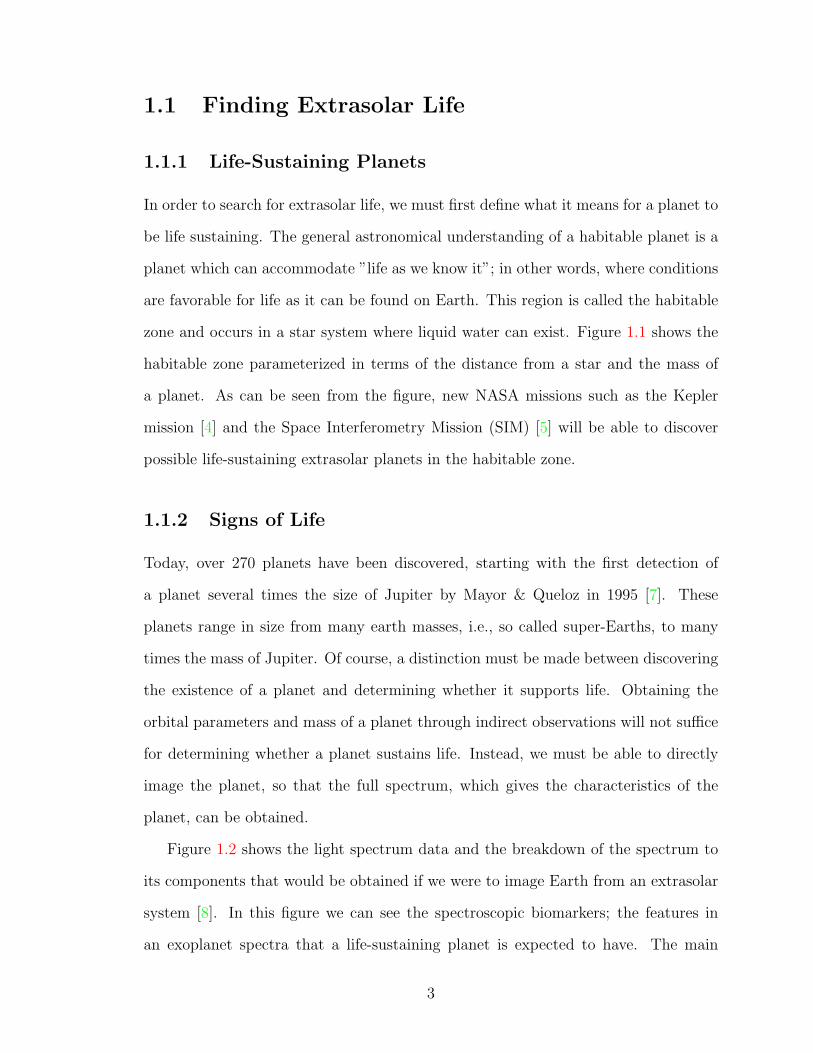
zone and occurs in a star system where liquid water can exist. Figure 1.1 shows the
habitable zone parameterized in terms of the distance from a star and the mass of
a planet. As can be seen from the figure, new NASA missions such as the Kepler
mission [4] and the Space Interferometry Mission (SIM) [5] will be able to discover
possible life-sustaining extrasolar planets in the habitable zone.
1.1.2 Signs of Life
Today, over 270 planets have been discovered, starting with the first detection of
a planet several times the size of Jupiter by Mayor & Queloz in 1995 [7]. These
planets range in size from many earth masses, i.e., so called super-Earths, to many
times the mass of Jupiter. Of course, a distinction must be made between discovering
the existence of a planet and determining whether it supports life. Obtaining the
orbital parameters and mass of a planet through indirect observations will not suffice
for determining whether a planet sustains life. Instead, we must be able to directly
image the planet, so that the full spectrum, which gives the characteristics of the
planet, can be obtained.
Figure 1.2 shows the light spectrum data and the breakdown of the spectrum to
its components that would be obtained if we were to image Earth from an extrasolar
system [8]. In this figure we can see the spectroscopic biomarkers; the features in
an exoplanet spectra that a life-sustaining planet is expected to have. The main
3
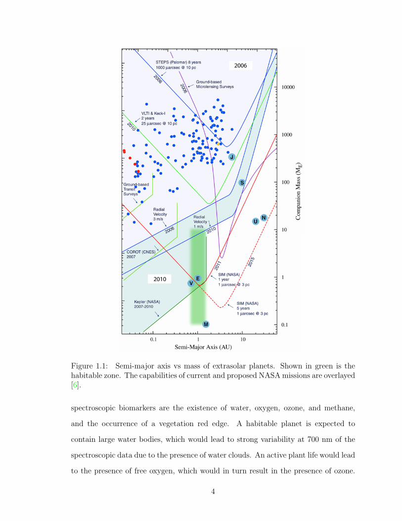
Figure 1.1: Semi-major axis vs mass of extrasolar planets. Shown in green is thehabitable zone. The capabilities of current and proposed NASA missions are overlayed[6].
spectroscopic biomarkers are the existence of water, oxygen, ozone, and methane,
and the occurrence of a vegetation red edge. A habitable planet is expected to
contain large water bodies, which would lead to strong variability at 700 nm of the
spectroscopic data due to the presence of water clouds. An active plant life would lead
to the presence of free oxygen, which would in turn result in the presence of ozone.
4

The atmosphere of planets with a low mass like Earth but without vegetation should
not contain methane due to stellar ultraviolet photodissociation; thus, its existence
would suggest a biological presence. As seen in figure 1.2, at around 750 nm, we
observe a vegetation red edge, which an Earth-like exoplanet might also exhibit [9]
[10].
Figure 1.2: Earthshine spectrum and its components Woolf et al. [8]. In the figure,I represents light intensity and λ wavelength.
1.1.3 Challenges associated with imaging planets in the hab-
itable zone
Most astronomers now suspect that rocky and possibly Earth-like planets orbit around
nearby stars. To date, all known planets have been discovered by indirect means,
that is, by measuring the motion of light from the parent star. These methods are
5

insensitive to the smaller terrestrial planets of interest and do not allow the most
ambitious characterization. In order to capture the signs of life from a planet we
need direct imaging of that planet.
As seen in figure 1.3, which simulates how the Solar System would be seen from
a distant star, the direct observation of Earth-like planets is extremely challenging
because their parent stars are about 1010 times brighter (in the visible spectrum) but
lie a fraction of an arcsecond away. Since the Earth atmosphere blurs the view of
the stars, telescopes that are stationed on Earth do not enable such high precision
imaging. Instead, space-based telescopy is required.
Figure 1.3: Simulation of light spectrum of the Sun and planets as seen from adistant star Des Marais et al. [11]. In the figure, I represents light intensity and λwavelength. ’Star’ stands for the Sun, and the solar planets are identified by theirinitial letters.
Many difficulties are involved in trying to achieve the high contrast necessary to
6
image a dim planet orbiting its parent star. Coronagraphy methods have been the
most promising solution to this problems to this date. Shown in figure 1.4 is the draw-
ing of the proposed NASA TPF-C mission (C stands for Coronagraph). Originally
invented by Bernard Lyot to image the corona of the sun [12], coronagraphy is an
optical technique which removes the starlight from the final image, while minimally
affecting the planet, or which modifies the point spread function of the system so
that the contrast is unity at the planet location. It consists of a dark spot at the
image used to block the central core of the Airy pattern and a smaller aperture at a
reimaged pupil to remove the residual stellar light. Building on this idea, different
types of coronagraph designs that would give the needed high-contrast images have
recently been designed at Princeton’s TPF group, which is headed by Jeremy Kasdin.
An example is shown in figure 1.4.
Figure 1.4: On the left, an artist’s illustration of the TPF-C spacecraft [13]. Onthe right, an optimized coronagraph pupil design by Vanderbei that can achieve theneeded contrast for exoplanet imaging if used with TPF-C [3].
The main challenge associated with designing a high-contrast imaging system is
the scattered light problem, which denotes the scattering of light in the final im-
age into the location of the planets point spread function due to aberrations in the
optics. Due to manufacturing imperfections, the surface figure of all mirrors and
lenses contains small variations from the desired shape, known as aberrations. This
7

negatively impacts imaging performance. Minor errors in reflectivity also affect the
quality of the final image. The combined amplitude and phase errors in the optics
typically degrade contrast by five or more orders of magnitude from the perfect optics
assumption. This becomes the critical design driver in any planet imaging telescope.
Until recently, solutions primarily focused on including an adaptive optics system in
the telescope. Such a system consists of multiple deformable mirrors that correct
the aberrated wavefront [14, 15]. Such a system measures the errors in the final im-
age, estimates the electric field, and computes corrections for the deformable mirrors.
Notwithstanding the recent progress in adaptive optics, such systems remain costly
and complex.
1.2 External Occulter for Exoplanet Imaging
An alternative approach to high-contrast imaging of extrasolar planets has been pro-
posed by Cash and Kasdin [9, 10, 16]. In this approach, an external screen or occulter
is used to block the wavefront from the star before it ever enters the telescope. The
poor diffraction performance of simple occulters has hitherto been an obstacle to
the wide acceptance of this approach. Fortunately, recent results in shaped-pupil
technology at Princeton have shown that these problems can be overcome with the
manufacture of a special starshade occulter. An example of a promising new occulter
design by Vanderbei, with a symmetric flower-shaped starshade, is shown in figure
1.5 [2]. This starshade is optimized for planet imaging by creating very high contrast
at small angles and suppressing the parent stars competing light. Since no starlight
can reflect off the surface aberrations, the need for wave-front control is eliminated.
Figure 1.6 shows a sketch of a sample occulter-based telescopy mission, consisting
of a roughly 50-m starshade flying 50,000 km from a conventional, 2-4-m diameter
telescope observatory [10]. The occulter significantly enhances the observatorys ca-
8

Figure 1.5: A multi-petal occulter design optimized for maximization of starlightsuppression [2].
Figure 1.6: Occulter-based extra-solar planet-finding mission diagram [16]
pabilities and lowers the exoplanet mission cost by avoiding the need for expensive
telescopes such as those required for suggested coronagraph and interferometer mis-
sions such as TPF-C and TPF-I. Because the occulter is not built into the telescope
as an add-on instrument, scattered light is reduced due to the existence of fewer op-
tical surfaces. This is due mainly to the fact that, as indicated above, the external
occulter circumvents the use of high-precision wavefront control in the optical design.
There are no unwanted diffraction spikes resulting from coronagraph supports, and
the complexity of telescope instruments, such as the small-scale imperfections in the
manufacturing and surfaces, is reduced. However, it introduces the difficult problem
of controlling and realigning the satellite formation.
As shown in figure 1.7, the baseline design of this mission suggests the placement of
9

Figure 1.7: A schematic diagram of occulter mission orbits projected into the eclipticplane [16]
.
an occulter satellite and a telescope near a Halo orbit about the Sun-Earth L2 point.
Spacecraft mission design around the L2 libration point has been used since the ISEE3
mission in 1978 due to its several advantages (see publications by Farquhar et al. for
more details [17, 18, 19, 20]). The energy level of the libration point orbits are close
to that of the Earth and the unstable manifold of L2 Halo orbits passes very close to
Earth. As a result, reaching these orbits is easy and requires minimal fuel. Since the
Sun, Earth and Moon are all in the same direction with respect to Sun-Earth L2 point,
half of the celestial sphere is available for imaging at any given time. The constant
distance to Earth also makes it relatively easier to keep communication with spacecraft
on L2 libration orbits than if it were on heliocentric drift-away orbits. Finally, L2 has
a stable thermal environment, which is a requirement for the temperature-sensitive
equipment – optical systems, lenses, and mirrors – on the telescopy mission under
study.
1.3 Dissertation Outline
This dissertation is presented in six chapters, the first of which is this introduction.
The remaining chapters are outlined below:
10
Chapter 2: Dynamical Analysis of the L2 Region
This chapter focuses on the underlying physics and qualitative behavior of the
natural dynamics of this system. I review the relevant literature on the bounded
motion of a small point-mass particle near the L2 point of the Circularly Re-
stricted Three Body Problem (CRTBP). These fuel-free orbits are useful as the
point of departure for the occulter mission design.
Chapter 3: Periodic Orbits of Interest Around L2: Numerical Methods
The horizontal Lyapunov, the vertical Lyapunov, and the Halo periodic orbits
around the L2 point are obtained numerically, and their stability properties are
examined. The real orbits in our solar system that correspond to these periodic
orbits of interest are then computed.
Chapter 4: Multiple Poincare Sections Method for Finding the Quasi-Halo
and Lissajous Orbits
Quasi-Halo orbits are good candidates for occulter placement, as they are fuel-
free orbits and have large sky coverage with respect to the Halo orbit, where
the telescope is placed. With the aim of identifying these orbits, I develop a
new numerical method that employs multiple Poincare sections to find quasi-
periodic orbits. This method converges to the desired orbits quickly, and it
exhibits robust behavior near chaotic regions. Its numerical implementation for
Lissajous and Quasi-Halo orbits are explained. These results are then extended
from the simplified three body model to find the orbits in the real solar system
that have the same characteristics.
Chapter 5: Finding the Optimal Trajectories
The optimal control problem of the realignment and Earth to Halo transfers is
solved. Different implementations, including the fuel- and time-optimal trajec-
tories that take the occulter from a given star Line-Of-Sight (LOS) to another
11
LOS, and from Earth to Halo, are numerically calculated using Euler Lagrange,
shooting and nonlinear programming approaches.
Chapter 6: Global Optimization of the Mission: The Traveling Salesman
Problem
The global optimization problem of finding the sequencing and timing of the
imaging sessions is examined. By including the telescopy constraints, the prob-
lem becomes a Dynamic Time-Dependent Traveling Salesman Problem (TSP)
with dynamical constraints. Simulated annealing and branching heuristic meth-
ods are employed to solve the TSP. Global optimization is performed for both
the single and multiple occulter missions. A feasibility study of the mission is
performed by analyzing possible scenarios with the capabilities of the SMART-1
spacecraft.
12
Chapter 2
Dynamical Analysis of the L2
Region
13
As discussed previously, the aim of this dissertation is to find the ”best” trajec-
tories for each spacecraft that is part of the occulter-based telescopy mission. In
three-dimensional space, this translates into the optimization of 3 × Ns/c control
forces in a 6 × (Ns/c + Ngb) dimensional dynamical system, where Ns/c and Ngb are
the number of spacecraft and gravitational bodies, respectively. In order to reduce
the complexity of the problem, I first analyze the control-free natural dynamics of a
single spacecraft under the simpler gravitational model.
This chapter focuses on the underlying physics and qualitative behavior of the
natural dynamics of this system. More specifically, I review the relevant literature
on the bounded motion of a small point-mass particle near the second Lagrange
point (also referred to as the libration point) of the Circular Restricted Three Body
Problem (CRTBP). This analysis helps identify the suitable regions of the phase space
for spacecraft placement.
In this chapter, I first derive the equations of motion for the CRTBP system
in a rotating frame. I then find the equilibrium points of this system. Linearizing
the equations of motion around the L2 equilibrium point, I categorize the types of
motion in the vicinity of the L2 point. Expanding the equations of motion in higher-
order Legendre polynomials, I apply the Lindstedt-Poincare procedure to obtain the
periodic halo orbits, which do not exist in the linearized system. I then apply the
center manifold reduction procedure to obtain the complete periodic phase space in
the extended L2 neighborhood. These fuel-free orbits provides the point of departure
for the occulter mission design.
14
2.1 Circularly Restricted Three Body Problem -
Equations of Motion
The Two-Body Problem, which can be solved analytically, describes the motion of
two bodies under the effect of their mutual gravitation interaction given their initial
conditions and masses [21, 22, 23]. There is no closed-form solution for the extension
of this problem to three bodies. Euler suggested a simplification of this Three-Body
Problem called the Circularly Restricted Three Body Problem (CRTBP) [24]. In the
CRTBP, the first two bodies, m1 and m2, called the primaries, are in circular motion
around their center of mass, which is the result of their mutual interaction based
on two-body gravitational dynamics. The third body, m3, which is free to move,
is assumed to be massless and hence to have no effect on the motion of the other
two bodies. The problem is to find the motion of the third body as determined by
the other two constrained bodies’ gravitational force. These assumptions reduce the
system’s degrees of freedom from nine to three, thereby increasing the tractability of
the solutions while still giving insightful information. The CRTBP is a useful model
for spacecraft mission design since the eccentricities of major planets in the Solar
system are small, and the mass of a spacecraft is negligible in comparison to the
celestial bodies.
In order to write the equations of motion under Newton’s law of gravitation, an
inertial frame of reference must be specified. The origin of the Newtonian inertial
frame, I, is located at the center of mass of m1 and m2, O. I has coordinates X, Y, Z,
such that the circular motion of the primaries is in the X,Y plane and the angular
rotation of the primaries is in the positive Z direction. Without loss of generality, we
assume that the first primary is heavier than the second primary, m1 > m2. In the
inertial frame I, the equation of motion of m3 under the gravitational forces of m1
15

and m2 is
m3d2~r
dt2
I
= −Gm1m3
‖~r1‖3~r1 −
Gm2m3
‖~r2‖3~r2 , (2.1)
where ~r1 and ~r2 are the relative positions of m3 with respect to m1 and m2, respec-
tively, and G is the universal gravitational constant.
Figure 2.1: Sketch of the CRTBP in the rotating frame R, where the Sun, S, is m1
and the Earth, E, is m2, and S/C refers to the spacecraft, m3.
In order to reduce the number of parameters and to generalize the solutions, the
variables of the problem are typically nondimensionalized. The unit of mass is chosen
as the total mass of the two main bodies, M = m1 +m2; the distance unit is chosen
as the distance between the two main bodies, D = ‖ ~d1‖+ ‖ ~d2‖; and the time unit is
chosen such that the period, T , of the circular motion is 2π. Under these choices, the
universal gravitational constant, G, becomes unity in order to enforce the two-body
period equality, T = 2π D3/2
M1/2G1/2 . Angular velocity, w = 2πT
, becomes unity as well. As
a result, the nondimensional system depends only on a single parameter. This is the
mass parameter, µ, defined as the ratio of the small body’s mass to the total mass:
16
µ = m2
M. Then, the nondimensional masses of the primaries can be expressed as
m1 = 1− µ (2.2)
m2 = µ . (2.3)
Since the distances of the primaries from the center of mass are inversely proportional
to their masses, the nondimensional distances can be expressed as
‖ ~d1‖ = µ (2.4)
‖ ~d2‖ = 1− µ . (2.5)
The nondimensionalized equation of motion becomes
d2~r
dt2
I
= −1− µ
‖~r1‖3~r1 −
µ
‖~r2‖3~r2 . (2.6)
In the inertial frame, I, the positions of the primaries are time dependent, making
the motion difficult to analyze. The time dependence of the equations of motion can
be eliminated by employing a rotating frame, R, with coordinates x, y, z. R is defined
with the origin at O; x directs from m1 to m2; y is perpendicular to x and lies in the
plane of the primaries’ motion; and z coincides with Z (see figure 2.1). R is called
the synodical frame.
In order to write the equations in R, the acceleration of m3 in the inertial coor-
dinates, d2~rdt2
I, should be expressed in terms of the rotating coordinate elements, x, y,
and z. The kinematical relationship between the acceleration in the inertial frame I
and the rotating frame R is
d2~r
dt2
I
= ~ω ×~r + ~ω × (~ω ×~r) + 2~ω × d~rR
dt+d2~r
dt2
R
, (2.7)
17
where ~ω is the angular velocity of the rotating frame. In the nondimensional units, ~ω
is equal to 1 · z; thus, the first term on the right hand side of equation 2.7 is nullified,
and the inertial acceleration is simplified to
d2~r
dt2
I
= (x− 2y − x) x+ (y + 2x− y) y + z z (2.8)
where the short-hand notation ˙ is used for the time derivative of a scaler. Plugging
equation 2.8 into equation 2.6, the final form of the equation of motion is obtained,
x = 2y + x− (1− µ)(x+ µ)
‖~r1‖3 − µ(x− 1 + µ)
‖~r2‖3
y = −2x+ y − (1− µ)y
‖~r1‖3− µy
‖~r2‖3
z = −(1− µ)z
‖~r1‖3 − µz
‖~r2‖3 . (2.9)
In these equations, the nondimensional positions with respect to the primaries are
~r1 = (x+ µ)x+ yy + zz (2.10)
~r2 = (x− 1 + µ)x+ yy + zz . (2.11)
Defining an effective potential, U(x, y, z), as
U(x, y, z) =1− µ
‖~r1‖+
µ
‖~r2‖+x2 + y2
2, (2.12)
the equations can be expressed in a simpler form,
x = 2y +∂U(x, y, z)
∂x
y = −2x+∂U(x, y, z)
∂y
z =∂U(x, y, z)
∂z. (2.13)
18

Defined by the differential equation 2.13, CRTBP has a first integral called the
Jacobi Constant, C, which is given by
C(x, y, z, x, y, z) = −(x2 + y2 + z2) + 2U + µ(1− µ). (2.14)
Differentiating C with respect to time, it can be observed that it is time invariant
and thus a constant of motion:
d
dtC = −2(xx+ yy + zz) + 2
d
dtU
= −2
((2y +
∂U
∂x)x+ (−2x+
∂U
∂y)y +
∂U
∂zz
)+ 2
d
dtU
= −2
(∂U
∂xx+
∂U
∂yy +
∂U
∂zz
)+ 2
d
dtU = 0 (2.15)
The existence of this integral of motion is due to the time-independent Lagrangian
nature of the CRTBP differential equation system (equation 2.13), which leads to
energy conservation (see [25] for details).
2.2 Equilibrium Points
At the equilibrium of a differential system, the state variables stay constant for all
time. Thus, in order to find the equilibrium points of CRTBP, all derivative terms in
equation 2.13 are set equal to zero:
0 =∂U
∂x= x− (1− µ)(x+ µ)
‖~r1‖3 − µ(x− 1 + µ)
‖~r2‖3 (2.16)
0 =∂U
∂y= y
(1− (1− µ)
‖~r1‖3− µ
‖~r2‖3
)(2.17)
0 =∂U
∂z= z
(−(1− µ)
‖~r1‖3 − µ
‖~r2‖3
). (2.18)
19

The five sets of values that satisfy these equations are called the Lagrange or the
libration equilibrium points. It is apparent from equation 2.18 that, at any equilibrium
point, z should be equal to zero. There are two possible solutions for equation 2.17;
y = 0 or y 6= 0. In the former case, there are three x values that satisfy equation 2.16
([24]). These are the collinear Lagrange points L1, L2, and L3 with coordinates
L1 = 1− µ− γ1, 0, 0 , (2.19)
L2 = 1− µ+ γ2, 0, 0 , (2.20)
L3 = −µ− γ3, 0, 0 . (2.21)
where γ1, γ2, and γ3 refer to the distances between the collinear Lagrange points and
their closest primaries. These are uniquely given by the positive roots of the following
quintic equations:
γ51 − (3− µ)γ4
1 + (3− 2µ)γ31 − µγ2
1 + 2µγ1 − µ = 0 , (2.22)
γ52 + (3− µ)γ4
2 + (3− 2µ)γ32 − µγ2
2 − 2µγ2 − µ = 0 , (2.23)
γ53 + (2 + µ)γ4
3 + (1 + 2µ)γ33 − (1− µ)γ2
3 − 2(1− 2µ)γ3 − (1− µ) = 0 . (2.24)
The other set of equilibrium points arise when y 6= 0. In this case, r1 = r2 = 1 should
be satisfied for equation 2.17 to hold. The positions of m1, m2, and m3 then form
an equilateral triangle. There are two equilibrium points that satisfy this constraint;
these are L4 and L5 with positions
L4 = µ− 1
2,
√3
2, 0 , (2.25)
L5 = µ− 1
2,−√
3
2, 0. (2.26)
20

Figure 2.2: Sketch of the locations of the Lagrange points [26]
2.3 Series Expansion around L2
While the ultimate aim is to characterize motion in the neighborhood of L2, analyt-
ical solutions are not available. I therefore proceed with asymptotic analysis, which
requires series expansion of the expressions on the right hand side of equation 2.13.
It is necessary to first change the variables such that the coordinates themselves are
small parameters. Subsequently, an appropriate expansion method is employed to
obtain the full series expressions.
2.3.1 Translation of L2 to the origin, and rescaling
In order to linearize CRTBP around the L2 point, which has the coordinates 1 −
µ + γ2, 0, 0, the equations must be written in a different set of coordinates, where
L2 is at the origin. In the next section, I will perform asymptotic analysis in the
neighborhood of L2, which extends from L2 to m2. Following Richardson [27], I
therefore change the unit of distance from D, the distance between the primaries, to
21

γ2, the distance from L2 to m2, since this is more in line with the length scales of the
problem. The distance unit rescaling ensures that the series expansions have good
numerical properties. In order to translate L2 to the origin and rescale the units, the
following change of variables is applied:
xnew =x− 1 + µ− γ2
γ2
(2.27)
ynew =y
γ2
(2.28)
znew =z
γ2
(2.29)
(2.30)
The mass unit is kept as M . Time unit is chosen such that the gravitational constant,
G, is unity in the new unit system as it was before. In the new time unit, the period
of the circular motion of the primaries, T , is 2π(
Dγ2
)3/2
, as a result of the Keplerian
period equation for the primaries, T = 2π D3/2
M1/2G1/2 . To simplify the equations, we
define a new variable, γL,
γL ,γ2
D.
Then, the period of the primaries is T = 2πγL− 3
2 , and the angular velocity, ω = 2πT
,
is γL32 . Change in the unit of time scales the time derivative operator, ˙, in the new
unit system by γL32 . To keep the differential equations consistent, we define a new
time variable, s,
s , γL
32 t ,
and a derivative with respect to this new time variable,
′ ,d
ds.
22
This notation enables the use of the old differential equations by only replacing, ˙,
with, ′ . From here on, subscripts for xnew, ynew and znew are dropped for convenience.
2.3.2 Series Expansion of the Equations
The right hand terms in the equations of motion, equation 2.13, are expanded using
the fact that
1
‖~r + ~ρ‖=
1
‖~r‖
∞∑n=0
Pn (cos(α))
(‖~ρ‖‖~r‖
)n
(2.31)
where Pn (·) are the Legendre polynomials, and
cos(α) =~ρ ·~r‖~ρ‖‖~r‖
. (2.32)
Defining ~ρ = x, y, z, distances to primaries can be written as
~r1 = (1
γL
+ 1)x+ ~ρ (2.33)
~r2 = x+ ~ρ . (2.34)
Using equations 2.31-2.34, the gravitation potential can be expanded in Legendre
polynomials around L2,
1− µ
‖~r1‖+
µ
‖~r2‖=
∞∑n>2
cnρnPn
(x
ρ
). (2.35)
where ρ = ‖~ρ‖ and the cn coefficients are
cn =(−1)n
γL3
(µ+
(1− µ)γLn+1
(1 + γL)n+1
). (2.36)
23

Thus, the series expansion for the effective potential, U , in equation 2.12 becomes
U =x2 + y2
2+
1− µ
‖~r1‖+
µ
‖~r2‖
=1
2
((1 + 2c2)x
2 + (1− c2)y2 − c2z
2)
+∞∑
n>3
cnρnPn
(x
ρ
). (2.37)
Substituting the new coordinates in equation 2.13 and employing the U expansion,
the equations of motion become:
x′′ − 2y′ − (1 + 2c2)x =∂
∂x
∞∑n>3
cnρnPn
(x
ρ
)=
∞∑n>2
(n+ 1)cn+1ρnPn
(x
ρ
)
y′′ + 2x′ + (c2 − 1)y =∂
∂y
∞∑n>3
cnρnPn
(x
ρ
)=
∞∑n>3
cnyρn−2Pn
(x
ρ
)
z′′ + c2z =∂
∂z
∞∑n>3
cnρnPn
(x
ρ
)=
∞∑n>3
cnzρn−2Pn
(x
ρ
), (2.38)
where
Pn =
[(n−2)/2]∑k=0
(3 + 4k − 2n)Pn−2k−2
(x
ρ
), (2.39)
and the bracket operator, [ ], gives the integer part of a real number.
2.4 Analysis of the Linear Part around L2
Before looking at the more complicated non-linear dynamical system, I investigate
the linearized system to gain insight into the stability and the structure of the phase
space. Ignoring the second and high-order terms in equation 2.38, the linear equations
24
of motion are
x′′ − 2y′ − (1 + 2c2)x = 0
y′′ + 2x′ + (c2 − 1)y = 0
z′′ + c2z = 0 . (2.40)
The linearized motion in the x−y plane and in the z direction are independent of one
another. For the purpose of our studies, which focus on the motion around the Earth-
Sun L2 with µ = 3.040423398444176 × 10⁻⁶, the c2 constant can be obtained from
equation 2.36 as 4.006810788883402. Noting that c2 > 0, motion in the z direction is
a simple harmonic oscillator. To study the in-plane motion, the differential equations
are written in the first-order form:
d
dt
x
y
x′
y′
=
0 0 1 0
0 0 0 1
(1 + 2c2) 0 0 2
0 −(c2 − 1) −2 0
x
y
x′
y′
. (2.41)
This system has four eigenvalues, which are
e1,2 = ±λ = ±√c2 − 2 +
√9c22 − 8c2√
2
e3,4 = ±iν = ±i√−c2 + 2 +
√9c22 − 8c2√
2, (2.42)
where λ and ν are positive constants. This can be shown through algebraic manip-
ulation for µ < 12
[24]. Thus, the planar system has two real eigenvalues, λ and −λ
, corresponding to the divergent and convergent modes, respectively, and, two imag-
inary eigenvalues, ±ν, corresponding to the oscillatory modes. The corresponding
25
eigenvectors for these modes are
~vλ =
1
−σ
λ
−λσ
, ~v−λ =
1
σ
−λ
−λσ
, ~v−ν =
1
ik
iν
−νk
, ~vν =
1
−ik
−iν
−νk
, (2.43)
where
σ =2λ
λ2 + c2 − 1and
k =ν2 + 2c2 + 1
2ν. (2.44)
The general solution to the linear ODE can then be written as:
x(s)
y(s)
x′(s)
y′(s)
= C1e
λs
1
−σ
λ
−λσ
+ C2e
−λs
1
σ
−λ
−λσ
+ C3
cos(νs)
−k sin(νs)
−ν sin(νs)
−νk cos(νs)
+ C4
sin(νs)
k cos(νs)
ν cos(νs)
−νk sin(νs)
.
(2.45)
The x− y plane has a center × saddle structure. This can be visualized by drawing
the projection of the motion in these subspaces onto the x-y coordinates, by ignoring
the velocity components (See figure 2.3). Including the z-direction mode, the linear
phase space around the L2 point has the center × center × saddle structure.
Saddle behavior around the Lagrange point can be utilized to design efficient
trajectories that veer in and out of the libration region for spacecraft missions. Fur-
thermore, analyzing the stable and unstable manifolds, it can be shown that there
exists a heteroclinic connection between the L1 and L2 points [28, 25]. This charac-
teristic is useful in mission design, such as the GENESIS mission trajectory to move
26

Figure 2.3: Projection onto the x-y coordinates of the saddle subspace (on the left)and center subspace (on the right) of the linearized planer motion around L2
between Sun-Earth L1 and L2 [29, 30].
Because this dissertation focuses on the types of motion that stay around the L2
region for all time, i.e. the libration orbits, this stable and unstable behavior will not
be analyzed further. Instead, I focus on the librational motion.
2.5 High-Order Analysis (The Lindstedt-Poincare
Procedure and Halo Orbits)
As seen above, there are periodic (and quasiperiodic) orbits near the collinear libration
points. I now turn to higher-order approximations for further insight.
Without loss of generality, if we restrict the initial conditions such that divergent
motion is not allowed, i.e. that the stable and unstable modes in the x-y plane are
excluded, we obtain the linear quasi-periodic orbits around L2, which can be written
in compact form as
x = −Axcos(νs+ φ)
y = kAxsin(νs+ φ)
z = Azcos(ωzs+ ψ) , (2.46)
27
where ωz =√c2. In the general case, when the in-plane and out-of-plane frequencies
are not commensurable, i.e., when νωz6= i1
i2where i1 and i2 are integers, Lissajous
orbits are obtained. In the linear analysis of the Earth-Sun CRTBP L2 point, these
frequencies,
ν = 2.073256862131411 and
ωz = 2.001701973042791 , (2.47)
are not commensurable. As a result, there are no three-dimensional periodic orbits
in the linear L2 system. However, as we move further away from the origin, and Ax
and Az increase, these amplitudes may affect the frequencies ν and ωz in a nonlinear
fashion. Since the frequencies in the x-y plane and in the z direction are very close
to one another, it makes intuitive sense to seek the possibility of 1-1 commensurate
nonlinear three-dimensional orbits. When the in-plane and out-of-plane frequencies
are equal, i.e. ν = ωz, 1-1 commensurable periodic orbits are obtained. These
orbits were first discovered by Farquhar, who coined the term “Halo” orbits due to
the resemblance of the Earth-Lunar L2 Halo orbits to a halo when seen from Earth
[31, 32, 33].
The linearized equations give the first approximation for this type of periodic
motion. In order to find the solutions for the Halo orbits up to the third order,
I use Richardson’s application of the Lindstedt-Poincare successive approximation
technique [27]. In the Lindstedt-Poincare procedure, the frequency correction for the
periodic motion is expanded in powers of the amplitude O(Anx),
ω = 1 +∑n>1
ωn, ωn < 1 , (2.48)
where the coefficients ωn are chosen to remove the secular terms at each step.
A new time variable, τ = ωs, is introduced, and the equations of motion 2.38 are
28

expanded up to the third order, which yields
ω2x′′ − 2ωy′ − (1 + 2c2)x =3
2c3(2x
2 − y2 − z2) + 2c4x(2x2 − 3y2 − 3z2) +O(4)
ω2y′′ + 2ωx′ + (c2 − 1)y = −3c3xy −3
2y(4x2 − y2 − z2) +O(4)
ω2z′′ + c2z = −c3xz −3
2z(4x2 − y2 − z2) +O(4) . (2.49)
It can be shown that the choice of
ω1 = 0 and ω2 = s1A2x + s2A
2z, (2.50)
removes the secular terms up to third order, with the requirement that in-plane and
out-of-plane amplitudes and phases satisfy the following conditions:
0 = l1A2x + l2A
2z + ∆
ψ = φ+ nπ
2, n = 1, 3 . (2.51)
For lengthy variables, l1, l2, s1, s2 and ∆, see [27]. From these equations, we see
that the smallest Halo orbit occurs when Az = 0, which, in the Sun-Earth L2 case,
corresponds to approximately Ax = 200, 000 km.
Using the frequency correction and the phase amplitude constraints, the third-
order solution of the Halo orbit is
x = a21A2x + a22A
2z − Axcos(τ1) + (a23A
2x − a24A
2z)cos(2τ1)
+ (a31A3x − a32AxA
2z))cos(3τ1)
y = kAxsin(τ1) + (b21A2x − b22A
2Z)sin(2τ1) + (b31A
3x − b32AxA
2z)sin(3τ1)
z = δn(Azcos(τ1) + d21AxAz(cos(2τ1)− 3)
+(d32AzA2x − d31A
3z)cos(3τ1)) , (2.52)
29

where
τ1 = ντ + φ ,
δn = 2− n, n = 1, 3 . (2.53)
Depending on the value of n, there are two types of Halo orbits, called the northern
(n = 1) and southern Halos (n = 3), which are the mirror images of each other with
respect to the x− y plane. This is due to the CRTBP’s mirror symmetry across the
z = 0 plane, that is, the equations of motion are invariant under the transformation:
x, y, z, x, y, z ⇒ x, y, −z, x, y, −z. Figure 2.4 shows an approximate northern
Halo orbit obtained via the Richardson formulation. While it is possible to extend
1.004 1.006 1.008 1.01 1.012 1.014 1.016
−5
−4
−3
−2
−1
0
1
2
3
4
5
X(AU)
Y(A
U)
1.006 1.007 1.008 1.009 1.01 1.011 1.012 1.013
−2
−1
0
1
2
3
X(AU)
Z(A
U)
−5 0 5−4
−3
−2
−1
0
1
2
3
4
Y(AU)
Z(A
U)
Figure 2.4: Sample northern Halo orbit approximation via the Richardson formula-tion.
this analysis further to higher orders (see [34]), the Richardson results are adequate
30

for a quantitative understanding of the Halo orbits and as an initial estimate for the
numerical procedure that will be used in the chapters to follow.
2.6 Reduction to Center Manifold
In the previous sections, I first looked at the linear phase space around L2, and then at
the higher-order series solutions to find an approximation for the Halo orbits. To gain
more insight into the periodic and quasi-periodic librational motions, I now turn to an
analysis of the full periodic subspace, i.e. the center manifold around L2. This can be
done by separating the periodic and divergent manifolds through the center manifold
reduction technique. This method is based on symplectic Lie-transformations on
the series expansion of the Hamiltonian. Here, I explain how the center manifold
reduction technique is applied to CRTBP, and I summarize the results obtained by
Jorba and Masdemont in [35, 36].
2.6.1 Transformation into complex normal form
Introducing new momenta,
px = x′ − y
py = y′ + x
pz = z′ , (2.54)
the corresponding Hamiltonian for equation 2.38 becomes
H=1
2(p2
x + p2y + p2
z) + ypx − xpy −∞∑
n=2
cnρnPn
(x
ρ
). (2.55)
31
To be able to apply the Lie series procedure, the quadratic part of the Hamiltonian,
which corresponds to the linear ODE, must be in the normal form,
H2 = λxpx + ν(y2 + py2) + ωz(z
2 + pz2) , (2.56)
where λ, ν and ωz are the eigenvalues of the linear ODE system as defined previously.
Analyzing the eigenvectors from the last section, it can be shown that the following
symplectic transformation takes H2 into the normal Hamiltonian form H2,
x
y
z
px
py
pz
=
2λs1
0 0 0 −2λs1
2νs2
0
λ2−2c2−1s1
ν2−2c2−1s2
0 λ−2c2−1s1
0 0
0 0 1√ωz
0 0 0
λ2+2c2+1s1
ν2+2c2+1s2
0 λ+2c2+1s1
0 0
λ3+(1−2c2)λs1
0 0 −λ3−(1−2c2)λs1
ν3+(1−2c2)νs2
0
0 0 0 0 0√ωz
x
y
z
px
py
pz
,
(2.57)
where,
s1 =√
2λ((4 + 3c2)λ2 + 4 + 5c2 − 6c22)
s2 =√ωz((4 + 3c2)ν2 − 4− 5c2 + 6c22) . (2.58)
32
Finally, H2 is transformed into the complex normal form in order to simplify the
symbolic numerical manipulations and to keep the notation concise.
q1
q2
q3
p1
p2
p3
=
1 0 0 0 0 0
0 1√2
0 0 − i√2
0
0 0 1√2
0 0 − i√2
0 0 0 1 0 0
0 − i√2
0 0 1√2
0
0 0 − i√2
0 0 1√2
x
y
z
px
py
pz
(2.59)
This transformation brings the quadratic Hamiltonian to its complex normal form,
H2(q, p) = λq1p1 + iνq2p2 + iωzq3p3 . (2.60)
Then the expanded Hamiltonian becomes:
H(q, p) = H2(q, p) +∑n>3
Hn(q, p)
= λq1p1 + iνq2p2 + iωzq3p3 +∑n>3
Hn(q, p) , (2.61)
where Hn is the nth order homogenous polynomial of the canonical coordinates and
momenta
Hn(q, p) =∑
‖k‖1=n
hknq
k11 q
k22 q
k33 p
k41 p
k52 p
k63 , (2.62)
and where the short notation k = k1, k2, k3, k4, k5, k6 is used with ‖ ‖1 as the usual
1-norm given by ‖k‖1 = |k1|+ |k2|+ |k3|+ |k4|+ |k5|+ |k6|.
33
2.6.2 The Procedure Explained
The aim of the center manifold reduction is to separate the motion of the center part
from the saddle part. This is achieved by applying successive canonical transforma-
tions to H, which results in the transformed Hamiltonian, H, whose exponents of q1
and p1 are always the same, i.e. k1 = k4. Eliminating all the polynomials, where
k1 6= k4 up to the Nth order, we obtain a new Hamiltonian of the following form,
H(q, p) = λq1p1 + iνq2p2 + iωzq3p3 +N∑
n>3
Hn(q1p1, q2, q3, p2, p3) +R(q, p) . (2.63)
It is easy to see that I = q1p1 is a first integral of motion when the effect of the
residue, R(q, p), is ignored. Using the fact that the time flow of this system is given
by Hamilton’s equations,
p = −∂H∂q
, q =∂H
∂p, (2.64)
the constancy of I can be observed by differentiating it:
dI
dt= q1
∂H
∂p1
− p1∂H
∂q1
= 0 . (2.65)
Hence, if I = 0 at time zero, it is zero for all time and the truncated Hamiltonian, H,
is constrained to be a function of only q2, q3, p2, and p3. The origin of the reduced
H(0, q2, q3, p2, p3) system is an elliptic equilibrium point. It is restricted to a manifold
tangent to linear center space, hence it is reduced to the center manifold.
34
2.6.3 Implementation of the Lie Series Method
Center manifold reduction is achieved by using successive canonical transformations,
which are almost identity, through the Lie Series method. This method uses the time
flow of a generating function, G, to canonically transform the original Hamiltonian
into H through the following Lie series:
H = H + [H,G] +1
2[[H,G], G] +
1
3![[[H,G], G], G] + . . . , (2.66)
where [ · , · ] is the Lie bracket operator. H is given in equation 2.61 and we want
H to be of the form given in equation 2.63. As a result, the problem is reduced to
finding G in the polynomial equation 2.66. Similar to the expansion of H via the
equations 2.61 and 2.62, H and G are expanded in power series with the notation,
G = G2 +G3 +G4 + ...
H = H2 + H3 + H4 + ... , (2.67)
where Hn and Gn are nth-order homogenous polynomials given as
Gn =∑
‖k‖1=n
gknq
k11 q
k22 q
k33 p
k41 p
k52 p
k63
Hn =∑
‖k‖1=n, k1=k4
hkn(q1p1)
k1qk22 q
k33 p
k52 p
k63 . (2.68)
The problem of finding the transformation is now converted into finding the coeffi-
cients gkn. Using the Lie bracket property that [Hn, Gm] is a homogeneous polynomial
of degree n +m− 2, the expanded equation is split up into polynomial equations of
35
increasing degrees:
H2 = H2
H3 = H3 + [H2, G3]
H4 = H4 + [H2, G4] + [H3, G3] +1
2[[H2, G3], G3]
... (2.69)
For k vector values with k1 6= k4, H is zero. Thus, the equations simplify to
0 = H3 + [H2, G3]
0 = H4 + [H2, G4] + [H3, G3] +1
2[[H2, G3], G3]
... (2.70)
For the first equation, the solution is
gk3 =
−hk
3
(k4−k1)λ+i(k5−k2)ν+i(k6−k3)ωzfor k1 6= k4 & ‖k‖1 = 3
0 otherwise.
(2.71)
Then, the equations given in 2.70 are solved sequentially to first find G3, then G4,
and so on, in order to obtain the generating function up to a finite truncated order.
Since k1 6= k4, the denominator term is non-zero, and the series solution diverges very
slowly.
Once the manifold reduction is complete and G and H have been obtained, the
qualitative structure of the center space can be analyzed. In the case of expansion
around L2, this manifold is four-dimensional and difficult to visualize. To visualize
the qualitative behavior on a two-dimensional figure, the system must be reduced
by two more dimensions. This is achieved by first restricting the system to a fixed
Hamiltonian and then taking a Poincare section through the surface q3 = 0. Now we
36
can see the projection of the system to two dimensions. Figure 2.5 shows a collection
of two-dimensional plots representing the dynamics in the periodic phase space with
different Hamiltonians.
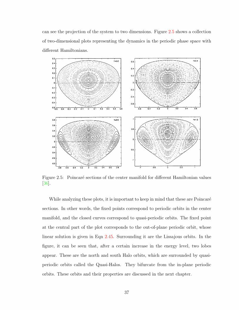
Figure 2.5: Poincare sections of the center manifold for different Hamiltonian values[36].
While analyzing these plots, it is important to keep in mind that these are Poincare
sections. In other words, the fixed points correspond to periodic orbits in the center
manifold, and the closed curves correspond to quasi-periodic orbits. The fixed point
at the central part of the plot corresponds to the out-of-plane periodic orbit, whose
linear solution is given in Eqn 2.45. Surrounding it are the Lissajous orbits. In the
figure, it can be seen that, after a certain increase in the energy level, two lobes
appear. These are the north and south Halo orbits, which are surrounded by quasi-
periodic orbits called the Quasi-Halos. They bifurcate from the in-plane periodic
orbits. These orbits and their properties are discussed in the next chapter.
37
Chapter 3
Periodic Orbits of Interest around
L2: Numerical Methods
38

The second chapter looked at the dynamical properties and the low-order analyt-
ical solutions for the periodic and quasi-periodic orbits around L2 for the simplified
CRTBP. In this chapter, I find the real orbits in our solar system that correspond
to these analyzed orbits. The chapter proceeds in two sections. The first section ex-
plains the numerical tools that are used to find the exact solutions and the stability
properties for the periodic orbits in the CRTBP. These methods are then applied to
find the horizontal Lyapunov, the vertical Lyapunov, and the Halo orbits, and their
stability properties.
3.1 Numerical Tools for Periodic Libration Orbits
around L2
Finding periodic orbits of a first order ODE system can be formulated as a boundary
value problem (BVP). Shooting algorithms were the first methods to be employed
to solve these types of BVPs. Their easy implementation and lack of computational
intensity ensures their continued popularity as BVP solving methods. Howell obtained
the Halo orbits numerically for the first time using a shooting method, [37].
The accurate analytical approximations for the periodic orbits of interest obtained
in the last chapter form the starting points of the numerical algorithms. While the
shooting method only uses one point from the analytical approximation, the collo-
cation method uses the whole approximation. This extra information ensures the
superior performance of the collocation algorithm. The collocation algorithms have
higher accuracy and a bigger region of attraction (minimal need of continuation pro-
cedure). In order to verify and confirm the correctness of the results, I implemented
both shooting and collocation algorithms to find the periodic orbits of interest.
In addition, as we will see in the last section of this chapter, the collocation
algorithm can be modified to transfer these orbits from the CRTBP to a full Solar
39

System model. For these reasons, I explain the implementation of the collocation
algorithms to the CRTBP periodic orbits and refer the reader to [37] for further
details on the shooting method.
3.1.1 Collocation as a Numerical Tool to Find Periodic Or-
bits
If a trajectory φ(t,x0) begins at a point x0 at time t = 0, and at some later time
t = T the trajectory φ(T,x0) returns to the point of departure, then this trajectory
is called a periodic orbit with period T . Finding periodic orbits of a first-order ODE
system can be formulated as a BVP. For a generic system, the problem mathematically
reduces to finding the solution x(t) of the autonomous ODE
x(t) = f(t,x) , (3.1)
within the time boundaries
0 6 t 6 T , (3.2)
where the system is subjected to boundary conditions which correspond to the peri-
odicity condition, i.e. the trajectory closing on itself:
g(x(0),x(T )) = x(0)− x(T ) = 0. (3.3)
After formulating the computation of the periodic orbit as a BVP, the state vector,
x(t), which is subjected to the differential equation and boundary constraints, is
solved. To implement the problem on a digital computer, the time and state variables
40

are discretized at N + 1 points along the trajectory
0 = t0 < t1 . . . < ti < . . . < tN−1 < tN = T ,
x0 = x(0), . . . , xi = x(ti), . . . , xN = x(T ) . (3.4)
Now, we need to find the discrete relationship that corresponds to the ODE
x(t)− f(t,x) = 0 ⇒ F (ti,xi, ti+1,xi+1) = 0 . (3.5)
There are schemes that can be used for this discretization. Among the most popular
are the Runge-Kutta formulas and the Simpson’s quadrature. Cash and his colleagues
have developed a number of effective solvers - for example, Cash and Wright TWBVP
[38, 39], where the basic formula is Simpson’s rule for quadrature. In the BVP solver
COLNEW, Ascher et al. [40, 41], implemented a family of implicit Runge-Kutta
methods. I used the Kierzenka et al.’s [42] bvp4c implementation, where a Simpson’s
formula for the quadrature is implemented. One advantage of this implementation is
that the discretized equations can be analytically solved without intermediate vari-
ables. If the initial guess is sufficiently close to the real solution, the discretized
Simpson quadrature equation, which corresponds to the differential equation, gives
the following constraint at every point:
F (xi) = −xi+1 + xi +hi
6(f(ti,xi) + f(ti+1,xi+1)) . . . (3.6)
+2hi
3f
(ti + ti+1
2,xi + xi+1
2− hi
8[f(ti,xi)− f(ti+1,xi+1)]
)] ,
where
hi = ti+1 − ti. (3.7)
41
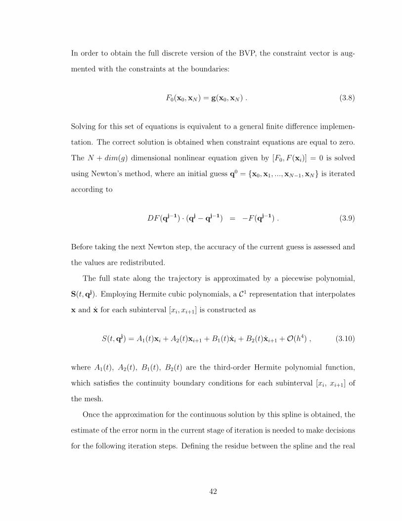
In order to obtain the full discrete version of the BVP, the constraint vector is aug-
mented with the constraints at the boundaries:
F0(x0,xN) = g(x0,xN) . (3.8)
Solving for this set of equations is equivalent to a general finite difference implemen-
tation. The correct solution is obtained when constraint equations are equal to zero.
The N + dim(g) dimensional nonlinear equation given by [F0, F (xi)] = 0 is solved
using Newton’s method, where an initial guess q0 = x0,x1, ...,xN−1,xN is iterated
according to
DF (qj−1) · (qj − qj−1) = −F (qj−1) . (3.9)
Before taking the next Newton step, the accuracy of the current guess is assessed and
the values are redistributed.
The full state along the trajectory is approximated by a piecewise polynomial,
S(t,qj). Employing Hermite cubic polynomials, a C1 representation that interpolates
x and x for each subinterval [xi, xi+1] is constructed as
S(t,qj) = A1(t)xi + A2(t)xi+1 +B1(t)xi +B2(t)xi+1 +O(h4) , (3.10)
where A1(t), A2(t), B1(t), B2(t) are the third-order Hermite polynomial function,
which satisfies the continuity boundary conditions for each subinterval [xi, xi+1] of
the mesh.
Once the approximation for the continuous solution by this spline is obtained, the
estimate of the error norm in the current stage of iteration is needed to make decisions
for the following iteration steps. Defining the residue between the spline and the real
42

solution as
r(t)j = S′(xj)− f(xj,S(xj)) , (3.11)
the error norm is calculated by integration of the residue between the spline and the
real solution by a 5-point Lobatto quadrature approximation [43] on each subinterval
i:
||r(xj)||i =
(∫ xi+1
xi
||r(xj)||2)1/2
. (3.12)
Based on the norm of the residual of the continuous solution, the mesh points, xj,
are redistributed. Extra points are added to the intervals with residues larger than
minimum error tolerance, and the points on the intervals which have errors much
smaller than the minimum tolerance are removed. Then, the Newton’s iteration is
continued until ||r(xj)|| < ε, where ε is a preset tolerance for the BVP solution. Then,
it is assumed that the iteration converged and that the correct answer is obtained.
3.1.2 Stability Analysis of Periodic Orbits
The stability of an orbit of a dynamical system determines whether nearby orbits
will stay in close proximity to that orbit or be repelled from it as time progresses.
The Poincare map enables us to determine the stability of a periodic orbit for a
time-independent dynamical system (for a detailed mathematical explanation, see
Guckenheimer & Holmes [44]). It does so by converting the n-dimensional continuous
dynamical system into an (n− 1)-dimensional map.
Let us consider surface section Σ, a subspace with a dimension lower than the
dynamical system of interest, that is transversal to the flow direction. A first return
map or Poincare map is the intersection of a periodic orbit, x(t), in the state space of
the continuous dynamical system with Σ. If we consider a periodic orbit with initial
43

conditions, x0, on the Poincare section and observe the successive points at which this
orbits returns to the section, xi, we can reduce the dynamical system to the following
map
xi+1 = P (xi) (3.13)
on the section Σ section. The periodic orbit of the dynamical system becomes the
fixed point of the map P when
x0 = P (x0) . (3.14)
Thus, the transformation converts the condition for the stability of the periodic orbit
to determining the stability of the map P . In order to study the stability of the
Poincare map, it is linearized around the fixed point
δxi+1 = DP (x0)δxi. (3.15)
The fixed point of this map, x0, is asymptotically stable if the moduli of all the
eigenvalues of DP are less than one and unstable if any of the eigenvalues are outside
the unit circle. The stability of the periodic orbit is determined by the fixed point of
the map.
Floquet theory offers an attractive numerical alternative to determining the sta-
bility of a periodic orbit without employing Poincare maps. Instead of using a section
in the phase space, we linearize the T-periodic vector field around the periodic or-
bit. Solving the linearized equations, we obtain the Floquet multipliers that define
the rate of convergence or divergence of small perturbations from the periodic orbit.
Guckenheimer and Holmes prove that one of the Floquet multipliers is unity with the
eigenvector corresponding to motion along the periodic orbit, and that the (n − 1)
44

eigenvalues of DP are equal to (n− 1) of the Floquet multipliers of the periodic orbit
[44].
In what follows, I investigate the stability of one particular periodic solution x(t)
with period T of the autonomous system given as: x = f(x). I proceed by linearizing
the T-periodic vector field around the periodic orbit φ(t, x0). First, let us note that
the trajectory satisfies its own ODE,
d
dt
∂φ(t, x0)
∂x0
= f(φ(t, x0)), with φ(0, x0) = x0 . (3.16)
Differentiating this equation with respect to x0, we obtain
d
dt
∂φ(t, x0)
∂x0
= Df(φ)∂φ(t, x0)
∂x0
, with initial condition∂φ(0; x0)
∂x0
= I. (3.17)
Rewriting equation 3.17 in terms of the state transition matrix, Φ(t), where Φ(t) :=
∂φ(t,x0)∂x0
, we obtain
Φ = Df(x)Φ, Φ(0) = I . (3.18)
The monodromy matrix, M , of a periodic solution, x(t), with period T and initial
condition x0, is defined as
M := Φ(T ) =∂φ(T, x0)
∂x0
. (3.19)
The eigenvalues of the monodromy matrix are the Floquet multipliers [44]. They
define the full stability properties of the periodic orbit of interest. We can see this by
looking at how much a perturbed trajectory φ(t, x0 +δx0) separates from the periodic
trajectory φ(t, x0) after one period.
δx(T ) = φ(T, x0 + δx0)− φ(T, x0) . (3.20)
45
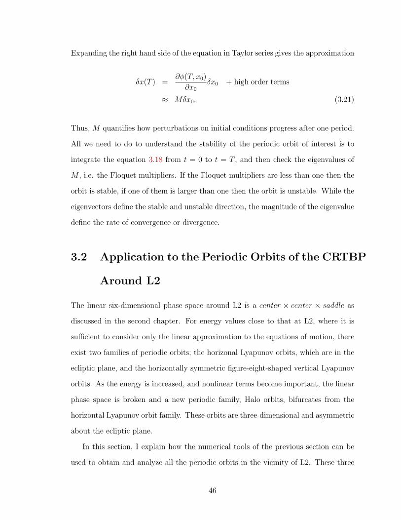
Expanding the right hand side of the equation in Taylor series gives the approximation
δx(T ) =∂φ(T, x0)
∂x0
δx0 + high order terms
≈ Mδx0. (3.21)
Thus, M quantifies how perturbations on initial conditions progress after one period.
All we need to do to understand the stability of the periodic orbit of interest is to
integrate the equation 3.18 from t = 0 to t = T , and then check the eigenvalues of
M , i.e. the Floquet multipliers. If the Floquet multipliers are less than one then the
orbit is stable, if one of them is larger than one then the orbit is unstable. While the
eigenvectors define the stable and unstable direction, the magnitude of the eigenvalue
define the rate of convergence or divergence.
3.2 Application to the Periodic Orbits of the CRTBP
Around L2
The linear six-dimensional phase space around L2 is a center × center × saddle as
discussed in the second chapter. For energy values close to that at L2, where it is
sufficient to consider only the linear approximation to the equations of motion, there
exist two families of periodic orbits; the horizonal Lyapunov orbits, which are in the
ecliptic plane, and the horizontally symmetric figure-eight-shaped vertical Lyapunov
orbits. As the energy is increased, and nonlinear terms become important, the linear
phase space is broken and a new periodic family, Halo orbits, bifurcates from the
horizontal Lyapunov orbit family. These orbits are three-dimensional and asymmetric
about the ecliptic plane.
In this section, I explain how the numerical tools of the previous section can be
used to obtain and analyze all the periodic orbits in the vicinity of L2. These three
46
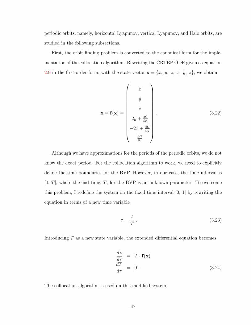
periodic orbits, namely, horizontal Lyapunov, vertical Lyapunov, and Halo orbits, are
studied in the following subsections.
First, the orbit finding problem is converted to the canonical form for the imple-
mentation of the collocation algorithm. Rewriting the CRTBP ODE given as equation
2.9 in the first-order form, with the state vector x = x, y, z, x, y, z, we obtain
x = f(x) =
x
y
z
2y + ∂U∂x
−2x+ ∂U∂y
∂U∂z
. (3.22)
Although we have approximations for the periods of the periodic orbits, we do not
know the exact period. For the collocation algorithm to work, we need to explicitly
define the time boundaries for the BVP. However, in our case, the time interval is
[0, T ], where the end time, T , for the BVP is an unknown parameter. To overcome
this problem, I redefine the system on the fixed time interval [0, 1] by rewriting the
equation in terms of a new time variable
τ =t
T. (3.23)
Introducing T as a new state variable, the extended differential equation becomes
dx
dτ= T · f(x)
dT
dτ= 0 . (3.24)
The collocation algorithm is used on this modified system.
47
After finding the periodic orbit, the stability analysis is conducted. The Jaco-
bian of the differential equation that is used in equation 3.18 to integrate the state
transformation, Φ, and find Monodromy matrix, M , is
Df =
0 I
U∗xx 2Ω
, (3.25)
where 0 is the 3×3 zero matrix, I is the 3×3 identity matrix, U∗xx is the matrix of
symmetric second partial derivatives of U with respect to x, y and z,
U∗xx =
Uxx Uxy Uxz
Uyx Uyy Uyz
Uzx Uzy Uzz
, (3.26)
and Ω is
Ω =
0 1 0
−1 0 0
0 0 0
. (3.27)
Now we define a new 42-dimensional augmented state vector consisting of the 6-
dimensional state vector and the 36-dimensional state transition matrix: xaug =
[x; Φ(:)]. Integrating the augmented state vector, M = Φ(T ) is obtained.
Before going into the details of each orbit calculation, I would like to point out
some of the properties of the eigenvalues of the monodromy matrix of the periodic
orbits of the CRTBP. Since this is a map, an eigenvalue of +1 indicates a stationary
mode, and an eigenvalue of modulus one indicates a rotational mode. An eigenvalue
of modulus greater than +1 indicates the exponentially growing mode and a modulus
less than one indicates an exponentially decaying mode. As the direction along the
48
periodic orbit will always come back to the same point on the map, M always has
+1 as an eigenvalue, with the corresponding eigenvector tangent to the periodic orbit
direction at x0. Since the CRTBP is an autonomous Hamiltonian system, it has an
energy integral, the Jacobi Constant, which means that the periodic orbits come in
families. Thus, there will be another stationary mode and another +1 eigenvalue of
M, which is in the direction of the periodic orbit family, and the eigenvalue +1 has
an algebraic multiplicity of at least two. Moreover, M is symplectic for autonomous
Hamiltonian systems. Hence, if λ is an eigenvalue of M , then λ−1, λ (conjugate of
λ), and λ−1 are also eigenvalues of M , with the same multiplicity. To sum up, at
least two of the eigenvalues of M will be +1 and the other four will have to be such
that the conjugate and the inverse of these eigenvalues have to be eigenvalues as well.
These properties are useful for the stability analysis of the CRTBP orbits.
3.2.1 Horizontal Lyapunov Orbits
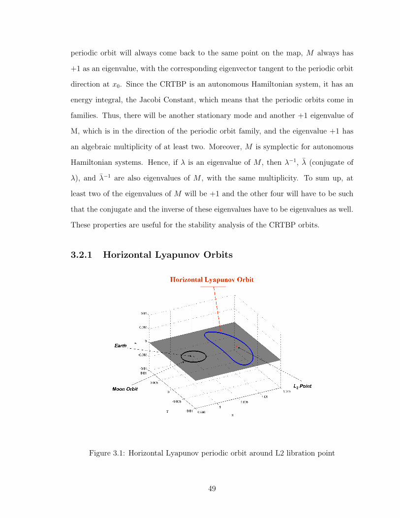
Figure 3.1: Horizontal Lyapunov periodic orbit around L2 libration point
49

The first type of periodic orbits are the horizontal Lyapunov orbits, which are con-
strained to the x-y plane. As a result, z = z = 0 throughout the trajectory. In
addition, the CRTBP dynamical system, which was defined in equation 3.22, is in-
variant under the transformation
x(t), y(t), z(t) ⇒ x(−t),−y(−t), z(−t) . (3.28)
Due to this invariance, the solution of the horizontal Lyapunov orbits will be sym-
metric with respect to the y plane and will cross the y plane perpendicularly [37].
Thus, at y(0) = 0, the periodic horizontal Lyapunov orbit has to satisfy
y(0) = 0, z(0) = 0, x(0) = 0, z(0) = 0 . (3.29)
These constraints simplify the problem such that for a given x(0) = x0, we only need
to find y(0) to specify a horizontal Lyapunov orbit. When choosing the boundary
condition, we need to be careful to avoid the degenerate solution, where x(0) = x(1)
with T = 0. However, the degenerate solution becomes infeasible if we set y(0) to a
constant value, y0, as the initial condition, instead of setting x(0) = x0. The constant
y0 is the orbit size parameter. Changing this parameter enables us to find periodic
orbits with different sizes and energies. Keeping these considerations in mind, I set
50

the boundary value problem as follows:
x(0) = x(1),
y(0) = y(1) = 0,
z(0) = z(1) = 0,
x(0) = x(1) = 0,
y(0) = y(1) = y0,
z(0) = z(1) = 0 . (3.30)
I then solve the BVP with the differential equation 3.24 and the boundary condition
equation 3.30, using the initial estimate from equation 2.45. Figure 3.1 shows a typical
horizontal Lyapunov periodic orbit around the Sun-Earth L2 point, which is found
with this method. By varying the y0 parameter, periodic orbits on different energy
levels are solved using collocation. The full horizontal Lyapunov family is obtained
as shown in figure 3.2.
0.98 0.99 1 1.01 1.02 1.03−0.06
−0.04
−0.02
0
0.02
0.04
0.06
X(AU)
Y(A
U)
Figure 3.2: Horizontal Lyapunov Family around L2
51
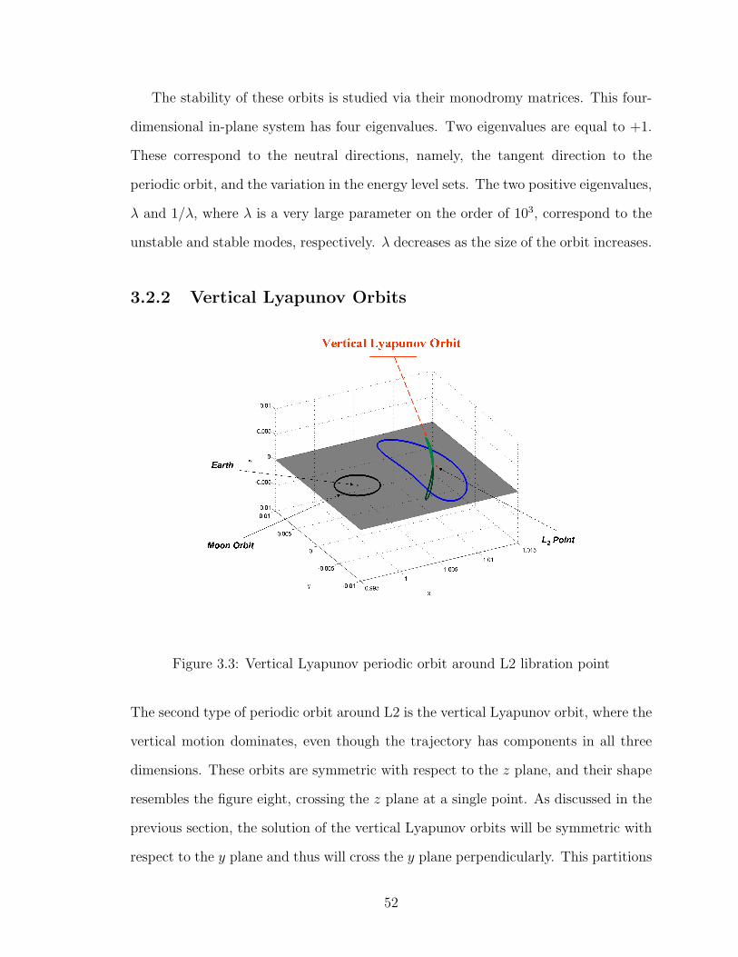
The stability of these orbits is studied via their monodromy matrices. This four-
dimensional in-plane system has four eigenvalues. Two eigenvalues are equal to +1.
These correspond to the neutral directions, namely, the tangent direction to the
periodic orbit, and the variation in the energy level sets. The two positive eigenvalues,
λ and 1/λ, where λ is a very large parameter on the order of 103, correspond to the
unstable and stable modes, respectively. λ decreases as the size of the orbit increases.
3.2.2 Vertical Lyapunov Orbits
Figure 3.3: Vertical Lyapunov periodic orbit around L2 libration point
The second type of periodic orbit around L2 is the vertical Lyapunov orbit, where the
vertical motion dominates, even though the trajectory has components in all three
dimensions. These orbits are symmetric with respect to the z plane, and their shape
resembles the figure eight, crossing the z plane at a single point. As discussed in the
previous section, the solution of the vertical Lyapunov orbits will be symmetric with
respect to the y plane and thus will cross the y plane perpendicularly. This partitions
52
the vertical Lyapunov orbit into four symmetric parts. Instead of obtaining the
whole orbit, it is thus sufficient to find one of the symmetric parts, and this reduces
the computation time. As the orbit crosses the y plane at time zero, the periodic
vertical Lyapunov orbit has to satisfy
y(0) = 0, x(0) = 0, z(0) = 0 . (3.31)
At t = 1/4, the orbit crosses the y and z planes
y(1/4) = 0, z(1/4) = 0, x(1/4) = 0 . (3.32)
As before, to avoid the degenerate solution, where x(0) = x(1/4) with T = 0, I specify
an initial condition that makes the degeneracy infeasible. I choose z(1/4) = z1/4 as
the orbit size parameter.
y(0) = y(1/4) = 0,
x(0) = x(1/4) = 0,
z(0) = 0,
z(1/4) = 0,
z(1/4) = z1/4 . (3.33)
I solve the BVP with differential equation 3.24 and the boundary condition equation
3.33, using the initial guess from equation 2.45. Figure 3.3 shows a typical vertical
Lyapunov periodic orbit around L2 found by using this method. By varying the z1/4
parameter, periodic orbits on different energy levels are solved using collocation and
the full vertical Lyapunov family is obtained as shown in figure 3.4.
53
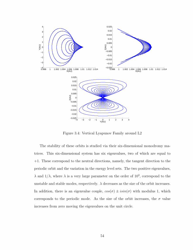
0.998 1 1.002 1.004 1.006 1.008 1.01 1.012 1.014−4
−3
−2
−1
0
1
2
3
4
X(AU)
Y(A
U)
0.998 1 1.002 1.004 1.006 1.008 1.01 1.012 1.014−0.025
−0.02
−0.015
−0.01
−0.005
0
0.005
0.01
0.015
0.02
0.025
X(AU)
Z(A
U)
−4 −3 −2 −1 0 1 2 3 4−0.025
−0.02
−0.015
−0.01
−0.005
0
0.005
0.01
0.015
0.02
0.025
Y(AU)
Z(A
U)
Figure 3.4: Vertical Lyapunov Family around L2
The stability of these orbits is studied via their six-dimensional monodromy ma-
trices. This six-dimensional system has six eigenvalues, two of which are equal to
+1. These correspond to the neutral directions, namely, the tangent direction to the
periodic orbit and the variation in the energy level sets. The two positive eigenvalues,
λ and 1/λ, where λ is a very large parameter on the order of 103, correspond to the
unstable and stable modes, respectively. λ decreases as the size of the orbit increases.
In addition, there is an eigenvalue couple, cos(σ) ± isin(σ) with modulus 1, which
corresponds to the periodic mode. As the size of the orbit increases, the σ value
increases from zero moving the eigenvalues on the unit circle.
54
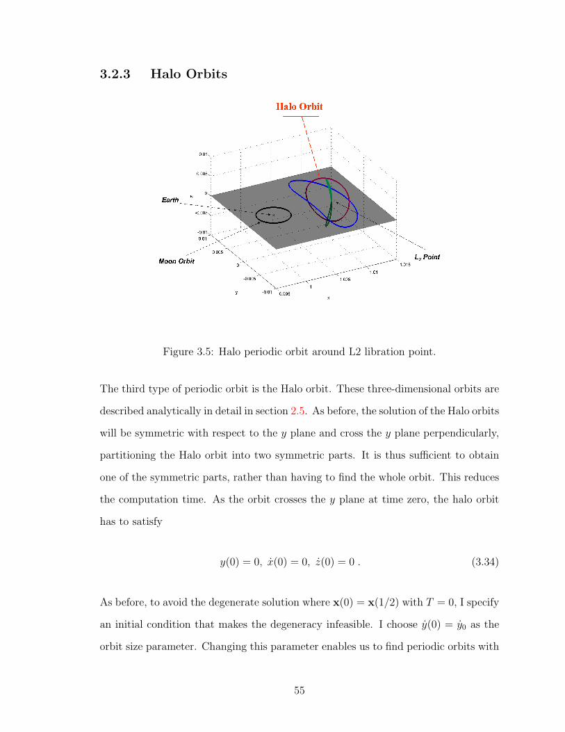
3.2.3 Halo Orbits
Figure 3.5: Halo periodic orbit around L2 libration point.
The third type of periodic orbit is the Halo orbit. These three-dimensional orbits are
described analytically in detail in section 2.5. As before, the solution of the Halo orbits
will be symmetric with respect to the y plane and cross the y plane perpendicularly,
partitioning the Halo orbit into two symmetric parts. It is thus sufficient to obtain
one of the symmetric parts, rather than having to find the whole orbit. This reduces
the computation time. As the orbit crosses the y plane at time zero, the halo orbit
has to satisfy
y(0) = 0, x(0) = 0, z(0) = 0 . (3.34)
As before, to avoid the degenerate solution where x(0) = x(1/2) with T = 0, I specify
an initial condition that makes the degeneracy infeasible. I choose y(0) = y0 as the
orbit size parameter. Changing this parameter enables us to find periodic orbits with
55

different energy levels. So, I set the boundary value problem as follows:
y(0) = y(1/2) = 0,
x(0) = x(1/2) = 0,
y(0) = y0,
z(0) = z(1/2) = 0 . (3.35)
I solve the BVP with differential equation 3.24 and the boundary condition equa-
tion 3.35, using the initial estimate from equation 2.52. Figure 3.5 shows a typical
northern Halo periodic orbit around L2 that was found with this method. By varying
the y0 parameter, periodic orbits on different energy levels are solved using collo-
cation, and the full northern Halo family is obtained, as shown in figure 3.6. The
CRTBP dynamical system, which is defined in equation 3.22, is invariant under the
transformation
x(t), y(t), z(t) ⇒ x(t), y(t),−z(t) . (3.36)
Due to this invariance,there is a mirror symmetry across the z = 0 plane. Therefore,
there is also a southern Halo orbit family which is the mirror copy of the northern
family with respect to the z plane (not shown on figure 3.6).
56
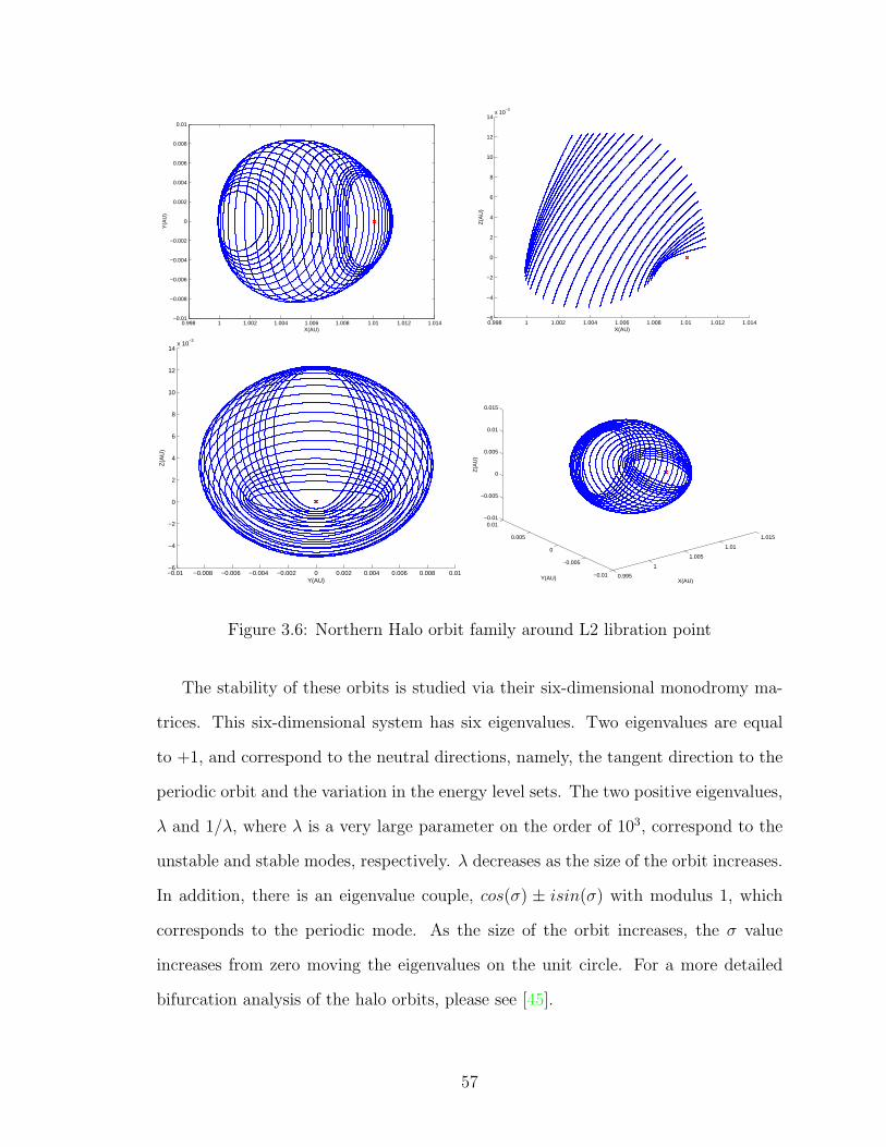
0.998 1 1.002 1.004 1.006 1.008 1.01 1.012 1.014−0.01
−0.008
−0.006
−0.004
−0.002
0
0.002
0.004
0.006
0.008
0.01
X(AU)
Y(A
U)
0.998 1 1.002 1.004 1.006 1.008 1.01 1.012 1.014−6
−4
−2
0
2
4
6
8
10
12
14x 10
−3
X(AU)
Z(A
U)
−0.01 −0.008 −0.006 −0.004 −0.002 0 0.002 0.004 0.006 0.008 0.01−6
−4
−2
0
2
4
6
8
10
12
14x 10
−3
Y(AU)
Z(A
U)
0.995
1
1.005
1.01
1.015
−0.01
−0.005
0
0.005
0.01−0.01
−0.005
0
0.005
0.01
0.015
X(AU)Y(AU)
Z(A
U)
Figure 3.6: Northern Halo orbit family around L2 libration point
The stability of these orbits is studied via their six-dimensional monodromy ma-
trices. This six-dimensional system has six eigenvalues. Two eigenvalues are equal
to +1, and correspond to the neutral directions, namely, the tangent direction to the
periodic orbit and the variation in the energy level sets. The two positive eigenvalues,
λ and 1/λ, where λ is a very large parameter on the order of 103, correspond to the
unstable and stable modes, respectively. λ decreases as the size of the orbit increases.
In addition, there is an eigenvalue couple, cos(σ) ± isin(σ) with modulus 1, which
corresponds to the periodic mode. As the size of the orbit increases, the σ value
increases from zero moving the eigenvalues on the unit circle. For a more detailed
bifurcation analysis of the halo orbits, please see [45].
57

Chapter 4
Multiple Poincare Sections Method
for Finding the Quasi-Halo and
Lissajous Orbits
58
There are three main challenges associated with finding quasi-periodic orbits. The
first is to minimize the time it takes to program the software that numerically solves
for the orbits. This reduces the threshold for researchers who work on trajectory
design. The second is to achieve reasonable execution times, allowing results to be
obtained quickly and “on the go”. The third is to improve the robustness of the
method in order to map the very large regions of attraction that are needed to obtain
the full families of quasi-periodic orbits.
Symbolic methods such as the Lindstedt-Poincare method by Gomez et al. [46]
and the reduction to the center manifold by Jorba et al. [36, 47], which depend
on series expansions, are very slow because an exponential increase in the number of
coefficients is needed for every additional increase in the order of expansion. The speed
problem can be overcome to a great extent by programming a symbolic manipulator
for the problem of interest, but this leads to a significant increase in programming
time. More importantly, some of these techniques have instability problems near
resonances.
This led to the consideration of fully numeric methods. However, instead of taking
a mesh on the whole surface, which requires many points and is thus memory and
CPU intensive, I considered only a section on the torus containing the quasi-periodic
trajectories, thus representing the full torus by only points on this section. This is
an invariant circle. These points on the invariant circle must be integrated for one
period at each iteration step. The initial errors in the estimation of the section increase
exponentially with the highest Lyapunov exponent as the integration time increases.
This is of great concern, especially for the CRTBP L2 case where the Lyapunov
exponent is more than 103. The effect is more dramatic near resonant and chaotic
regions. To overcome this problem, I reduce the integration times by taking multiple
sections on the torus, integrating only between the consecutive Poincare sections. The
methodology is parallel to the multiple shooting method used in two-point boundary
59

value problems [48].
This chapter consist of four sections. In the first section, I explain the main
idea of the procedure without going into details of the numerical implementation.
Here, I first introduce the methodology by explaining the procedure for a single
Poincare section. The results are then extended to multiple Poincare sections. I
discuss different implementations using various Poincare surfaces. A continuation
method to find the full family of quasi-periodic orbits is introduced.
In the second section, numerical details for obtaining the real quasi-periodic orbits
around L2 are explained.
The third section presents the results section, where I give the solutions for the
quasi-periodic orbits around L2 of the CRTBP, the Lissajous and the Quasi-Halo
orbits, and show the full periodic family and compare the results with the literature.
In the last section, I explain and apply the numerical method to ”transfer” these
orbits from the CRTBP model to the real ephemeris model of the Solar System.
This chapter is based on previous work by Kolemen and Kasdin [49].
4.1 Procedure
4.1.1 Finding Invariant Tori via a Single Poincare Section
For the occulter-based telescopy mission under study, the main quasi-periodic orbits
of interest are the Quasi-Halos which lie on two-dimensional invariant manifold. As
discussed in the introductory section, the multiple Poincare section procedure aims
to reduce the problem of finding the two-dimensional invariant manifold of the full
ordinary differential equation to finding the invariant circles, i.e., the one-dimensional
invariant manifold of the Poincare map. These invariant circles compactly define the
full two-dimensional manifold.
The first step in the single Poincare section procedure is to find a convenient
60
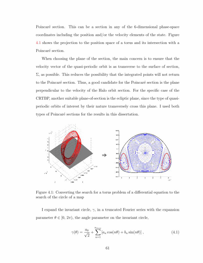
Poincare section. This can be a section in any of the 6-dimensional phase-space
coordinates including the position and/or the velocity elements of the state. Figure
4.1 shows the projection to the position space of a torus and its intersection with a
Poincare section.
When choosing the plane of the section, the main concern is to ensure that the
velocity vector of the quasi-periodic orbit is as transverse to the surface of section,
Σ, as possible. This reduces the possibility that the integrated points will not return
to the Poincare section. Thus, a good candidate for the Poincare section is the plane
perpendicular to the velocity of the Halo orbit section. For the specific case of the
CRTBP, another suitable plane-of-section is the ecliptic plane, since the type of quasi-
periodic orbits of interest by their nature transversely cross this plane. I used both
types of Poincare sections for the results in this dissertation.
Figure 4.1: Converting the search for a torus problem of a differential equation to thesearch of the circle of a map
I expand the invariant circle, γ, in a truncated Fourier series with the expansion
parameter θ ∈ [0, 2π), the angle parameter on the invariant circle,
γ(θ) =a0√2
+nmax∑n=1
[an cos(nθ) + bn sin(nθ)] , (4.1)
61
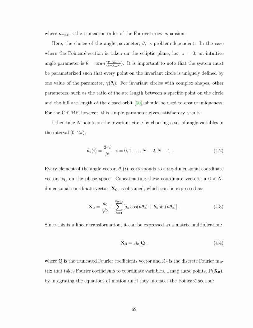
where nmax is the truncation order of the Fourier series expansion.
Here, the choice of the angle parameter, θ, is problem-dependent. In the case
where the Poincare section is taken on the ecliptic plane, i.e., z = 0, an intuitive
angle parameter is θ = atan( y−yhalo
x−xhalo). It is important to note that the system must
be parameterized such that every point on the invariant circle is uniquely defined by
one value of the parameter, γ(θi). For invariant circles with complex shapes, other
parameters, such as the ratio of the arc length between a specific point on the circle
and the full arc length of the closed orbit [50], should be used to ensure uniqueness.
For the CRTBP, however, this simple parameter gives satisfactory results.
I then take N points on the invariant circle by choosing a set of angle variables in
the interval [0, 2π),
θ0(i) =2πi
Ni = 0, 1, . . . , N − 2, N − 1 . (4.2)
Every element of the angle vector, θ0(i), corresponds to a six-dimensional coordinate
vector, xi, on the phase space. Concatenating these coordinate vectors, a 6 × N -
dimensional coordinate vector, X0, is obtained, which can be expressed as:
X0 =a0√2
+nmax∑n=1
[an cos(nθ0) + bn sin(nθ0)] . (4.3)
Since this is a linear transformation, it can be expressed as a matrix multiplication:
X0 = Aθ0Q , (4.4)
where Q is the truncated Fourier coefficients vector and Aθ is the discrete Fourier ma-
trix that takes Fourier coefficients to coordinate variables. I map these points, P(X0),
by integrating the equations of motion until they intersect the Poincare section:
62
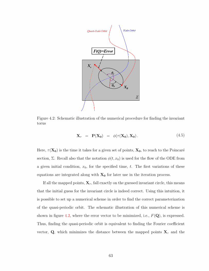
Figure 4.2: Schematic illustration of the numerical procedure for finding the invarianttorus
Xτ = P(X0) = φ(τ(X0),X0) . (4.5)
Here, τ(X0) is the time it takes for a given set of points, X0, to reach to the Poincare
section, Σ. Recall also that the notation φ(t, x0) is used for the flow of the ODE from
a given initial condition, x0, for the specified time, t. The first variations of these
equations are integrated along with X0 for later use in the iteration process.
If all the mapped points, Xτ , fall exactly on the guessed invariant circle, this means
that the initial guess for the invariant circle is indeed correct. Using this intuition, it
is possible to set up a numerical scheme in order to find the correct parameterization
of the quasi-periodic orbit. The schematic illustration of this numerical scheme is
shown in figure 4.2, where the error vector to be minimized, i.e., F (Q), is expressed.
Thus, finding the quasi-periodic orbit is equivalent to finding the Fourier coefficient
vector, Q, which minimizes the distance between the mapped points Xτ and the
63

invariant circle. This condition can be written in mathematical terms as:
F (Q) = Xτ − AθXτQ = 0 . (4.6)
Here, θXτ is the projection of the mapped points onto the invariant circle, which is
described in detail in section 4.2.3, and AθXτis the Fourier coefficient matrix, which
has the same structure as Aθ0 , but uses the projected angle elements instead of the
original ones.
One advantage of this formulation is that a Newton iteration can be used, which
has the potential to lead to quadratically convergent solutions. In Newton’s iteration,
an initial guess Q0 is iterated according to
DF(Qj) (Qj+1 −Qj) = −F (Qj) (4.7)
until a satisfactory answer is reached. Here, the superscript defines the value of Q at
a given iteration step. To find an explicit form for this equation, all its variables are
expanded in terms of Q. F then becomes:
F (Q) = Xτ −Xθφ(τ,X0)
= φ(τ, Aθ0 Q)− Aθφ(τ,Aθ0Q)
Q .
(4.8)
I then take the derivative with respect to Q:
DF(Q) = dXτ
dX0
dX0
dQ− dX
dθφ
dθφ
dXτ
dXτ
dX0
dX0
dQ
= DP Aθ0 − (DAθφ(τ,Aθ0Q)
Q)dθφ
dXτDP Aθ0 ,
(4.9)
where DP is the differential of the Poincare map that is obtained from the first
64
Figure 4.3: Iteration procedure in steps
variation of the map that was integrated with X. Employing Newton’s iteration,
solutions converge usually within 3-4 iterations. An example of an iteration procedure
is shown in figure 4.3. Here, the sample points are shown as crosses and the return
maps are represented by circles. After four iterations, all the sample points and the
return maps are aligned on the same invariant circle.
4.1.2 Extension to Multiple Poincare Sections
In order to overcome the potential instability that results from the long integration
times, the invariant torus is cut by several Poincare sections, as mentioned before.
Figure 4.4 shows the invariant circles which are obtained when the tori of interest
are cut with multiple sections. As a result, all the invariant circles in figure 4.4 are
65
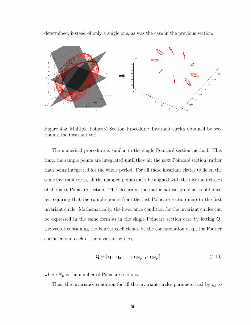
determined, instead of only a single one, as was the case in the previous section.
Figure 4.4: Multiple Poincare Section Procedure: Invariant circles obtained by sec-tioning the invariant tori
The numerical procedure is similar to the single Poincare section method. This
time, the sample points are integrated until they hit the next Poincare section, rather
than being integrated for the whole period. For all these invariant circles to lie on the
same invariant torus, all the mapped points must be aligned with the invariant circles
of the next Poincare section. The closure of the mathematical problem is obtained
by requiring that the sample points from the last Poincare section map to the first
invariant circle. Mathematically, the invariance condition for the invariant circles can
be expressed in the same form as in the single Poincare section case by letting Q,
the vector containing the Fourier coefficients, be the concatenation of qi, the Fourier
coefficients of each of the invariant circles,
Q = [q1; q2; . . . ; qNp−1; qNp ] , (4.10)
where Np is the number of Poincare sections.
Thus, the invariance condition for all the invariant circles parameterized by qi to
66

be on the same torus is
F (Q) = F
q1
q2
...
qNp−1
qNp
=
φ(τ, Aθ0 q1)
φ(τ, Aθ0 q2)
...
φ(τ, Aθ0 qNp−1)
φ(τ, Aθ0 qNp)
−
Aθφ(τ,Aθ0q1)
q2
Aθφ(τ,Aθ0q2)
q3
...
Aθφ(τ,Aθ0qNp−1)
qNp
Aθφ(τ,Aθ0qNp
)q1
= 0.(4.11)
Finally, as before, we apply Newton’s iteration to the root finding problem:
DF(Qj) (Qj+1 −Qj) = −F (Qj). (4.12)
4.1.3 Different Implementations
The quasi-periodic orbits reside in six-dimensional phase space, which has a four-
dimensional center manifold (periodic subspace). Each quasi-periodic orbit is of di-
mension two. Thus, two properties of a given quasi-periodic orbit must be specified
in order to uniquely define it. Many different parameters can be used to specify a
quasi-periodic orbit; among these, the most intuitive and relevant for mission design
are the Hamiltonian (or the Jacobi constant) of the orbit, the period of the orbit, and
the size of the orbit. Since prescribing the period also prescribes the Hamiltonian
and vice versa, two implementations where the period or the Hamiltonian is preset
are considered in this section.
When the Hamiltonian is used to specify a quasi-periodic orbit, another constraint
is needed in order to define the properties of the orbit of interest. I chose to specify
the size of the orbit as the second variable. This is a relevant parameter since the
distance between the telescope and the occulter is set by the size of the Quasi-Halo
orbit. Since the numerical method is based on Poincare sections, size can be specified
by the two-dimensional area, A, which is enclosed by the invariant circle. Then, the
67
constraint vector is augmented to include the new constraints:
F = [F ; Hfixed − HQ ; Afixed − AQ]. (4.13)
Another implementation is to set the period of the quasi-periodic orbit to a con-
stant. Quasi-Halo orbits have two periods; one around the Halo orbit and the other
along the Halo orbit. The period along the Halo orbit is very important for space
missions that require all spacecraft to stay close to one another at all times. An
uncontrolled mismatch in this period would lead to a separation on the order of the
size of the Halo orbit, which is unacceptable. However, this period for a numerically
computed two-dimensional structure is vague, unlike the one-dimensional case. I de-
fine this period of the Quasi-Halo to be the average time it takes for all the sample
points starting from the initial Poincare section to return back to it. That is, the
period is
T =1
n
n∑i=1
τ(xi) . (4.14)
Here, n is the total number of sample points taken on the Poincare section. This
way, the period of the quasi-periodic orbit can be specified along with the integration
direction for the return map. In this case, there is one more degree of freedom to
specify a unique orbit. Choosing the Hamiltonian as a constraint is not an option, as
discussed before. Thus, I specify the size of the orbit by choosing the area parameter:
the two-dimensional area, A, which is enclosed by the invariant circle. This can be
done by augmenting the error vector with a new constraint, such as the projected size
along one direction:
F = [F ; Tfixed − TQ ; Afixed − AQ ]. (4.15)
68
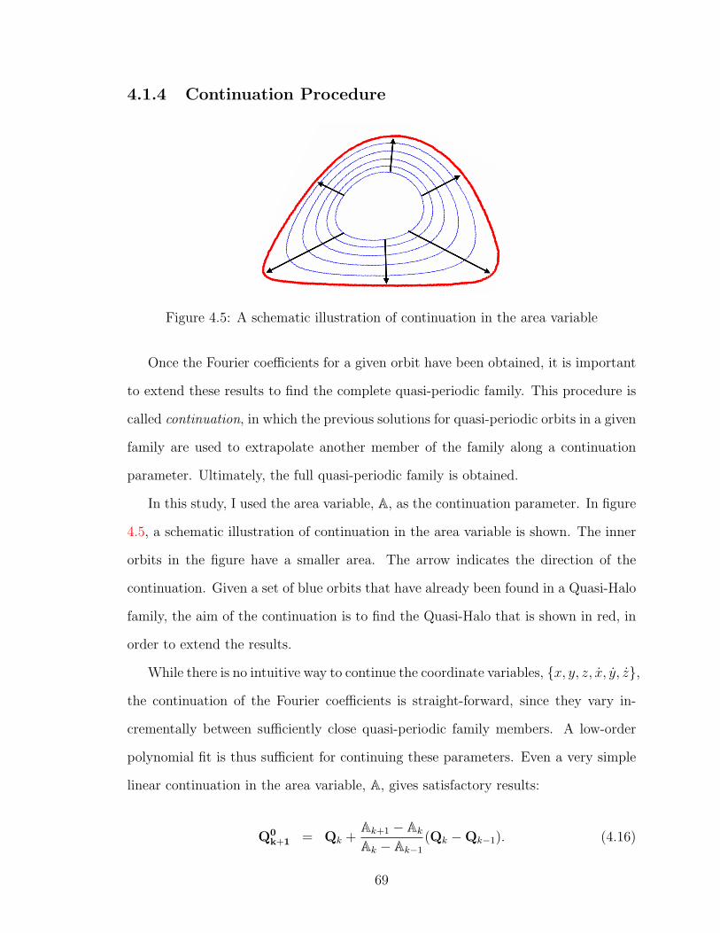
4.1.4 Continuation Procedure
Figure 4.5: A schematic illustration of continuation in the area variable
Once the Fourier coefficients for a given orbit have been obtained, it is important
to extend these results to find the complete quasi-periodic family. This procedure is
called continuation, in which the previous solutions for quasi-periodic orbits in a given
family are used to extrapolate another member of the family along a continuation
parameter. Ultimately, the full quasi-periodic family is obtained.
In this study, I used the area variable, A, as the continuation parameter. In figure
4.5, a schematic illustration of continuation in the area variable is shown. The inner
orbits in the figure have a smaller area. The arrow indicates the direction of the
continuation. Given a set of blue orbits that have already been found in a Quasi-Halo
family, the aim of the continuation is to find the Quasi-Halo that is shown in red, in
order to extend the results.
While there is no intuitive way to continue the coordinate variables, x, y, z, x, y, z,
the continuation of the Fourier coefficients is straight-forward, since they vary in-
crementally between sufficiently close quasi-periodic family members. A low-order
polynomial fit is thus sufficient for continuing these parameters. Even a very simple
linear continuation in the area variable, A, gives satisfactory results:
Q0k+1 = Qk +
Ak+1 − Ak
Ak − Ak−1
(Qk −Qk−1). (4.16)
69

Here, as before, the superscript of Q defines the Newton’s iteration step, while the
subscript defines the continuation step.
Once the initial guess for Q0k+1 is obtained, the multiple Poincare section method
is applied on this guess to get the correct Qk+1. Then, the continuation is repeated
to find Qk+2.
4.2 Numerical Application for the Quasi-Periodic
Orbits Around the L2 Region of the CRTBP
In this section, I show the numerical computation in implementation order. The
details of the computations are discussed in the sections that follow.
1. Compute the initial guess Q00.
2. Compute X0.
X0 = Aθ0 Qjk (4.17)
3. Compute Poincare map for each Σi.
Xτ = P (X0) (4.18)
4. Compute θXτ .
θXτ = arctan(Xτ (2)Xτ (1)
) for Lissajous orbits
θXτ = arctan(Xτ (6)Xτ (5)
) for Quasi-Halo orbits(4.19)
70

5. Compute the error.
F(Qi
k
)= Xτ − AθXτ
Qjk
(4.20)
6. Compute the Jacobian of the error.
DF(Qjk) = DP Aθ0 − (DAθXτ
Qjk)
dθφ
dXτDP Aθ0
(4.21)
7. Augment the error vector and the Jacobian.
F = [F ; Afixed − AQ ; . . .] ,
DF = [DF ; DA ; . . .] (4.22)
8. Perform Newton’s iteration.
DF(Qjk) (Qj+1
k −Qjk) = −F (Qj
k) (4.23)
9. Decision step:
Decision:
Qk = Qj+1
k and go to 10 if |F (Qjk)| < ε,
Go to 2 if j < jmax and |F (Qjk)| > ε
Redo 10 otherwise.
10. Continuation: Extrapolate an initial guess for Q0k+1 from previous Fourier ele-
ments Q0, . . . ,Qk and continuation variables A0, . . . ,Ak
Q0k+1 = polyfunc(Ak+1) . (4.24)
71
Stop the numerical implementation if the full quasi-periodic family is obtained.
Otherwise, go to 2.
4.2.1 Initial estimate for Q
Let us consider the monodromy matrix, M , which was discussed in the last chapter,
as a linear map from the initial variations around the periodic orbit at time 0 to
variation after one period T ,
M := δx0 → δxT . (4.25)
Recall that the monodromy matrices for vertical Lyapunov and Halo orbits each have
an eigenvalue couple, cosσ ± isinσ with modulus 1 and corresponding eigenvector
v1 ± iv2. By the definition of eigenvalue and eigenvector,
M (v1 + iv2) = (cosσ + isinσ) (v1 + iv2)
= cosσ v1 − isinσ v2 + i(sinσ v1 + cosσ v2) , (4.26)
M (v1 − iv2) = (cosσ − isinσ) (v1 − iv2)
= cosσ v1 − isinσ v2 − i(sinσ v1 + cosσ v2) . (4.27)
Using these properties, it is possible to find the invariant circle of the map M . Let
us consider a closed curve, ϕ, of this map, parameterized with θ = [0, 2π],
ϕ(θ) = κ(cosθv1 − sinθv2) . (4.28)
72

Using trigonometric manipulation, it can now be shown that the monodromy matrix
maps this closed curve onto itself:
ϕ(θ)M→ M κ(cosθ v1 − sinθ v2)
= κ(cos(θ + ρ) v1 − sin(θ + ρ) v2)
= ϕ(θ + ρ) . (4.29)
Thus, ϕ(θ) is a periodic orbit of this map (which should not be confused with the
invariant circle of the Poincare section) with κmagnitude. It is a linear approximation
to the relative distance from the quasi-periodic orbit to the periodic orbit. In the
numerical scheme, I used the linear approximation with small κ as the starting point
for the multiple Poincare scheme. κ values of order 10−6 have been sufficiently small
to give reasonable startup approximations. (Please recall that, in the normalized
units, 1 is the distance between Sun and Earth).
ϕ(θ) is a periodic orbit of the monodromy map. I first chose a high number,
NM = 100, of parametrization variables,
θM(i) =2πi
NM
i = 0, 1, . . . , Nm − 2, Nm − 1 , (4.30)
and obtained the corresponding NM points on the closed curve:
XM = ϕ(θM) . (4.31)
For the multiple Poincare algorithm, an initial estimate is needed for the periodic
orbit on the Poincare map. To this aim, I integrated XM and found their intersection
with the Poincare sections of interest. The methods I employed are the subject of the
two chapter sections that follow.
The initial estimate for the Fourier elements, Q00, was obtained by using fast
73
Fourier transform (fft) on the intersecting points. It is important to note that this
is the only time that a Fourier transform is employed in the algorithm. Once Q00
is obtained, all the transformations, including the continuation step, take Q → X.
For ease of programming, I chose to use real valued Fourier coefficients rather than
imaginary ones. Below, a pseudo-code shows how to obtain the Fourier coefficients:
input: X
N= length(X);
y = fft(X);
Q(1) = 1/sqrt(2)/N*real(y(1));
for i=2:i_max
Q(2*(i-1))= 2/N*real(y(i));
Q(2*(i-1)+1)= -2/N*imaginary(y(i));
output: Q
where i max was chosen to be 20. I would like to note that, due to sin(0)=0, the
imaginary part of y(1) is always 0.
4.2.2 Choosing the Poincare Section Surfaces
When choosing the planes of the section, the main concern is to ensure that the
velocity vector of the quasi-periodic orbit is as transverse to the surface of section, Σ,
as possible. This reduces the possibility of the integrated points not returning to the
Poincare section.
For the Lissajous orbits, I restrict the Poincare sections to be on one side of the
z = 0 plane because of the mirror symmetry of the CRTBP with respect to the z
plane, which was discussed in the previous chapters. For the single Poincare section
method, I used a section on the z = 0 plane. When extending this to multiple
Poincare sections, an intuitive choice was to use sections parallel to this z = 0. Thus,
74
I chose four sections over the half period (equivalent to seven sections over the full
period). Two of these are z = 0 and the other two are z = zfixed, one section as the
trajectories cross these sections in one direction and another while they cross in the
other direction:
0 = gi(x) = zfixedi− zqh(τi) . (4.32)
I chose zfixed to be half of the maximum displacement in the z-direction to ensure
that all the trajectories are transversal.
For Quasi-Halos, sections that are parallel to one another cannot be considered,
since the torus twists in space. A good candidate for the Poincare section surface,
g(x), is the plane perpendicular to the velocity of the halo orbit section:
0 = gi(x) = [xh(ti)− xqh(τi)]xh + [yh(ti)− yqh(τi)]yh + [zh(ti)− zqh(τi)]zh ,(4.33)
where subscript h stands for the Halo orbit and subscript qh stands for the Quasi-Halo
orbit.
Along the Quasi-Halo, ten of these sections, gi=0...9, are taken with equal separation
in time, i.e., ti = i9T
, where i = 0, . . . , 9. Figure 4.6 shows the multiple Poincare
sections on a sample Quasi-Halo orbit. Then, the Fourier coefficients that correspond
to all the sections along the trajectory are continued, giving initial conditions to the
next Quasi-Halo.
4.2.3 Choosing θ and computing its derivative dθXτ
dXτ
I choose the Poincare sections to be along the coordinate variables of the state. Thus,
an intuitive choice for θ would be to pick it as the angle between the coordinate
variables of the invariant circles. Since all the sections, gi(x) = zfixedi− zqh(τi), for
the Lissajous case are parallel to one another, it is feasible to choose θ as the angle
75
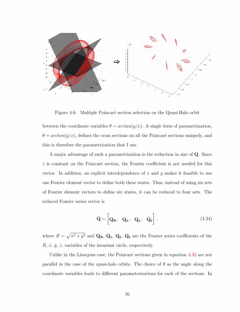
Figure 4.6: Multiple Poincare section selection on the Quasi-Halo orbit
between the coordinate variables θ = arctan(y/x). A single form of parametrization,
θ = arctan(y/x), defines the cross sections on all the Poincare sections uniquely, and
this is therefore the parametrization that I use.
A major advantage of such a parametrization is the reduction in size of Q. Since
z is constant on the Poincare section, the Fourier coefficient is not needed for this
vector. In addition, an explicit interdependence of x and y makes it feasible to use
one Fourier element vector to define both these states. Thus, instead of using six sets
of Fourier element vectors to define six states, it can be reduced to four sets. The
reduced Fourier series vector is
Q =
[QR ; Qx ; Qy ; Qz
], (4.34)
where R =√x2 + y2 and QR, Qx, Qy, Qz are the Fourier series coefficients of the
R, x, y, z, variables of the invariant circle, respectively.
Unlike in the Lissajous case, the Poincare sections given in equation 4.33 are not
parallel in the case of the quasi-halo orbits. The choice of θ as the angle along the
coordinate variables leads to different parameterizations for each of the sections. In
76

order to reduce the extra complication that this would entail, I opted for a simpler
parametrization that works for all the sections at the same time, as in the Lissajous
case. Figure 4.7 shows the projection of the invariant circle on different axes of all
the closed orbits on the Poincare sections. Looking at this figure, it is apparent that
parametrization θ = arctan(z/y) works for all the sections. As with the Lissajous
case, a major advantage of such a parametrization is the reduction in size of Q. The
reduced Fourier series vector for a quasi-halo is thus
Q =
[Qx ; Qy ; Qz ; Qx ; QR
], (4.35)
where R =√y2 + z2 and Qx, Qy, Qz, Qx, QR are the Fourier series coefficients of
the x, y, z, x, R variables of the invariant circle, respectively.
−5 0 5−6
−4
−2
0
2
4
6
X
Y
−5 0 5−10
−8
−6
−4
−2
0
2
4
6
8
X
Z
−6 −4 −2 0 2 4 6−10
−8
−6
−4
−2
0
2
4
6
8
Y
Z
−8 −6 −4 −2 0 2 4 6 8−2.5
−2
−1.5
−1
−0.5
0
0.5
1
1.5
2
2.5
Vx
Vy
−8 −6 −4 −2 0 2 4 6 8−2.5
−2
−1.5
−1
−0.5
0
0.5
1
1.5
2
2.5
Vx
Vz
−3 −2 −1 0 1 2 3−2.5
−2
−1.5
−1
−0.5
0
0.5
1
1.5
2
2.5
Vy
Vz
Figure 4.7: The relative distance from the invariant circle is projected on different
axes for a sample orbit. The upper three sub-plots show the projection on the position
space, while the lower ones show the projection on the velocity space. The sub-plot
on the lower right corner, which is the Vy (i.e. y) versus Vz (i.e. z), is highlighted in
red.
77
Finally, employing the chain rule, the derivative of θ with respect to Xτ can be
obtained as
dθXτ
dXτ
= [− y
x2 + y2,
x
x2 + y20, 0, 0, 0, ] for Lissajous
dθXτ
dXτ
= [ 0, 0, 0, 0, − z
y2 + z2,
y
y2 + z2] for Quasi-Halo .
4.2.4 Computing Aθ and DA
Recall that the invariant circle, γ, on the Poincare section was defined via a finite
Fourier series:
γ(θ) =a0√2
+nmax∑n=1
[an cos(nθ) + bn sin(nθ)] , (4.36)
with θ on the interval [0, 2π). and Aθ as the transformation from the Fourier elements
to the state vector.
In this section, I explain how to obtain this matrix and its derivative. The Fourier
coefficients vector, Q, for Lissajous and Quasi-Halo orbits was defined in equations
4.34 and 4.35. The state vector, X, can then be obtained by multiplying Q with the
following Aθ:
Aθ =
Asection1 0 · · · 0 0
0 Asection2 · · · 0 0
......
. . . 0 0
0 0 0 AsectionNsec−10
0 0 0 0 AsectionNsec
. (4.37)
In the above equation, the maximum number of sections, Nsec, is four for Lissajous
78
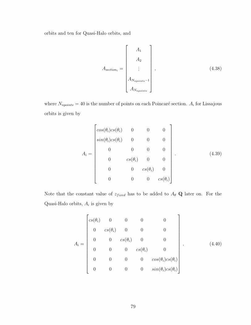
orbits and ten for Quasi-Halo orbits, and
Asectioni=
A1
A2
...
ANnpoints−1
ANnpoints
, (4.38)
where Nnpoints = 40 is the number of points on each Poincare section. Ai for Lissajous
orbits is given by
Ai =
cos(θi)cs(θi) 0 0 0
sin(θi)cs(θi) 0 0 0
0 0 0 0
0 cs(θi) 0 0
0 0 cs(θi) 0
0 0 0 cs(θi)
. (4.39)
Note that the constant value of zfixed has to be added to Aθ Q later on. For the
Quasi-Halo orbits, Ai is given by
Ai =
cs(θi) 0 0 0 0
0 cs(θi) 0 0 0
0 0 cs(θi) 0 0
0 0 0 cs(θi) 0
0 0 0 0 cos(θi)cs(θi)
0 0 0 0 sin(θi)cs(θi)
, (4.40)
79

where cs(θi) is the vector
cs(θi) =
12
cos(θi) sin(θi) cos(2θi) sin(2θi) · · · cos(N0θi) sin(N0θi)
.(4.41)
In the equation above, N0 = 20 is the maximum number of Fourier elements to
be used in the system. DA = dAθ
dθcan be obtained in a similar fashion. To save
space, I do not include the explicit form of DA. It can be obtained via term-by-term
differentiation of Aθ.
4.2.5 Augmenting the error vector F and its derivative DF
One of the main advantages of this algorithm is the ease with which constraints can
be added. For example, in order to fix the value of the Hamiltonian (i.e. the Jacobi
constant), equation 4.13 is used to augment the error vector, where Hfixed is set to
the Hamiltonian of the base Halo or the vertical Lyapunov orbit. The equation to
obtain the Hamiltonian is listed in 2.14.
Figure 4.8: Polar coordinates integration region [51].
As for the determination of the area variable, A, use of the Fourier coefficients is
of great help. If R denotes the region enclosed by a curve r(θ), as shown in figure
80
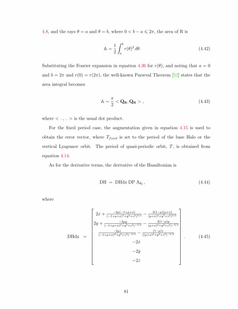
4.8, and the rays θ = a and θ = b, where 0 < b− a 6 2π, the area of R is
A =1
2
∫ b
a
r(θ)2 dθ. (4.42)
Substituting the Fourier expansion in equation 4.36 for r(θ), and noting that a = 0
and b = 2π and r(0) = r(2π), the well-known Parseval Theorem [52] states that the
area integral becomes
A =π
2< QR,QR > , (4.43)
where < . , . > is the usual dot product.
For the fixed period case, the augmentation given in equation 4.15 is used to
obtain the error vector, where Tfixed is set to the period of the base Halo or the
vertical Lyapunov orbit. The period of quasi-periodic orbit, T , is obtained from
equation 4.14.
As for the derivative terms, the derivative of the Hamiltonian is
DH = DHdx DP Aθ0 , (4.44)
where
DHdx =
2x+ −2µ(−1+µ+x)
(−1+µ+x)2+y2+z2)3/2 − 2(1−µ)(µ+x)
(µ+x)2+y2+z2)3/2
2y + −2µy(−1+µ+x)2+y2+z2)−3/2 − 2(1−µ)y
(µ+x)2+y2+z2)−3/2
−2µz(−1+µ+x)2+y2+z2)−3/2 − (1−µ)z
((µ+x)2+y2+z2)−3/2
−2x
−2y
−2z
. (4.45)
81
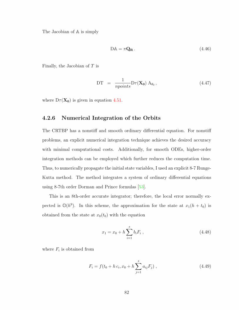
The Jacobian of A is simply
DA = πQR . (4.46)
Finally, the Jacobian of T is
DT =1
npointsDτ(X0) Aθ0 , (4.47)
where Dτ(X0) is given in equation 4.51.
4.2.6 Numerical Integration of the Orbits
The CRTBP has a nonstiff and smooth ordinary differential equation. For nonstiff
problems, an explicit numerical integration technique achieves the desired accuracy
with minimal computational costs. Additionally, for smooth ODEs, higher-order
integration methods can be employed which further reduces the computation time.
Thus, to numerically propagate the initial state variables, I used an explicit 8-7 Runge-
Kutta method. The method integrates a system of ordinary differential equations
using 8-7th order Dorman and Prince formulas [53].
This is an 8th-order accurate integrator; therefore, the local error normally ex-
pected is O(h9). In this scheme, the approximation for the state at x1(h + t0) is
obtained from the state at x0(t0) with the equation
x1 = x0 + h
s∑i=1
biFi , (4.48)
where Fi is obtained from
Fi = f(t0 + h ci, x0 + h
s∑j=1
aijFj) , (4.49)
82
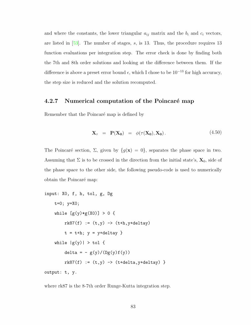
and where the constants, the lower triangular aij matrix and the bi and ci vectors,
are listed in [53]. The number of stages, s, is 13. Thus, the procedure requires 13
function evaluations per integration step. The error check is done by finding both
the 7th and 8th order solutions and looking at the difference between them. If the
difference is above a preset error bound ε, which I chose to be 10−13 for high accuracy,
the step size is reduced and the solution recomputed.
4.2.7 Numerical computation of the Poincare map
Remember that the Poincare map is defined by
Xτ = P(X0) = φ(τ(X0),X0) . (4.50)
The Poincare section, Σ, given by g(x) = 0, separates the phase space in two.
Assuming that Σ is to be crossed in the direction from the initial state’s, X0, side of
the phase space to the other side, the following pseudo-code is used to numerically
obtain the Poincare map:
input: X0, f, h, tol, g, Dg
t=0; y=X0;
while [g(y)*g(X0)] > 0
rk87(f) := (t,y) -> (t+h,y+deltay)
t = t+h; y = y+deltay
while |g(y)| > tol
delta = - g(y)/(Dg(y)f(y))
rk87(f) := (t,y) -> (t+delta,y+deltay)
output: t, y.
where rk87 is the 8-7th order Runge-Kutta integration step.
83

Each iteration of the last loop corresponds to performing a Newton iteration to
find a zero of the function F := g(φ(delta, y)) = 0 with initial condition delta = 0.
In this case, DF = dgdφ(delta,y)
dφ(delta,y)ddelta
. Remembering the Euler approximation to
integration, φ(delta, y) ≈ y + f(y) delta, I obtain DF = Dg(y) f(y). It is possible
to see that the pseudo-code employs root finding via the Newton iteration, delta =
−F DF−1. At the end of the algorithm, P (X0) = y and τ(X0) = t.
4.2.8 Numerical Computation of the Derivative of the Poincare
map
The differential of the Poincare map is computed as
DP(x) =d
dxφ(τ(x),x)) =
d
dτφ(τ(x),x) + Dφ(τ(x),x)
= f(P (x))Dτ(x) + Dφ(τ(x),x) , (4.51)
where the differential of the time to reach Σ is obtained by differentiating the Poincare
section condition,
0 = g(P (x))
⇒ = Dg(P(x))DP(x)
= Dg(P(x)) [f(P(x))Dτ(x) + Dφ(τ(x),x)]
= [Dg(P(x))f(P(x))] Dτ(x) + Dg(P(x))Dφ(τ(x),x)
⇒ Dτ(x) = −Dg(P(x))φ(τ(x),x))
Dg(P(x))f(P(x))(4.52)
Substituting equation 4.52 in equation 4.51, I obtain the final form of DP:
DP(x) = −f(P(x))Dg(P(x))φ(τ(x),x))
Dg(P(x))f(P(x))+ Dφ(τ(x),x)) . (4.53)
84
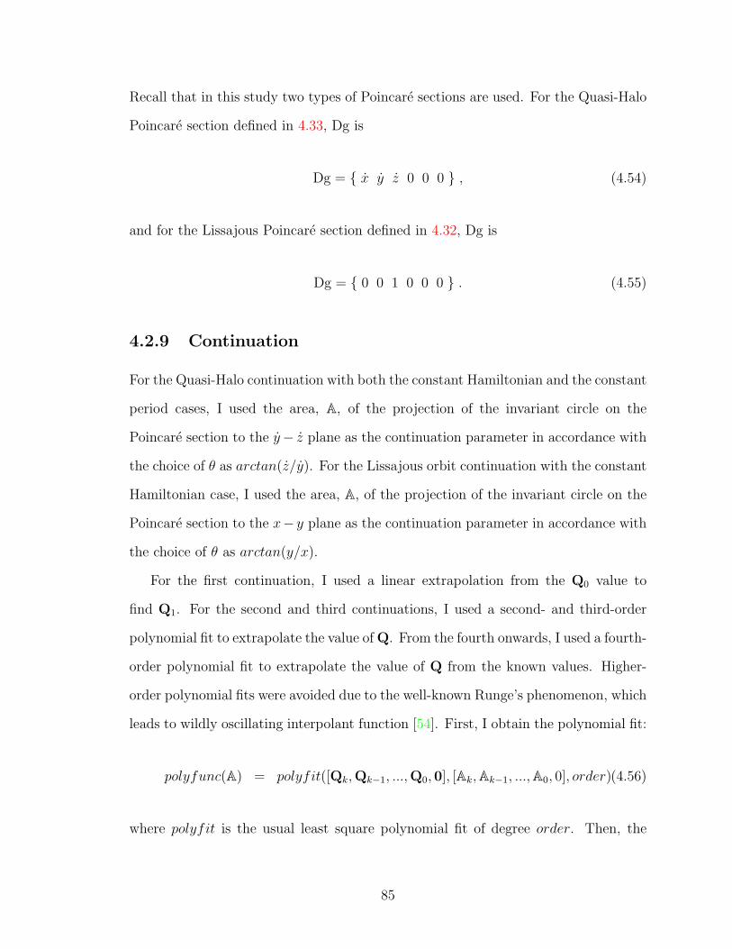
Recall that in this study two types of Poincare sections are used. For the Quasi-Halo
Poincare section defined in 4.33, Dg is
Dg = x y z 0 0 0 , (4.54)
and for the Lissajous Poincare section defined in 4.32, Dg is
Dg = 0 0 1 0 0 0 . (4.55)
4.2.9 Continuation
For the Quasi-Halo continuation with both the constant Hamiltonian and the constant
period cases, I used the area, A, of the projection of the invariant circle on the
Poincare section to the y− z plane as the continuation parameter in accordance with
the choice of θ as arctan(z/y). For the Lissajous orbit continuation with the constant
Hamiltonian case, I used the area, A, of the projection of the invariant circle on the
Poincare section to the x− y plane as the continuation parameter in accordance with
the choice of θ as arctan(y/x).
For the first continuation, I used a linear extrapolation from the Q0 value to
find Q1. For the second and third continuations, I used a second- and third-order
polynomial fit to extrapolate the value of Q. From the fourth onwards, I used a fourth-
order polynomial fit to extrapolate the value of Q from the known values. Higher-
order polynomial fits were avoided due to the well-known Runge’s phenomenon, which
leads to wildly oscillating interpolant function [54]. First, I obtain the polynomial fit:
polyfunc(A) = polyfit([Qk,Qk−1, ...,Q0,0], [Ak,Ak−1, ...,A0, 0], order)(4.56)
where polyfit is the usual least square polynomial fit of degree order. Then, the
85

continuation of the Fourier coefficient is performed by extrapolation:
Qk+1 = polyfunc(Ak+1) , (4.57)
where
Ak+1 = Ak + ∆A . (4.58)
While choosing ∆A, there is a compromise between speed and convergence. The
larger the ∆A, the shorter the continuation procedure takes, while the possibility of
non-convergence increases with increasing step size. To find the optimal iteration
step size automatically, I set
∆A =
1.2 ∆A if Newton iteration converged for all previous cases
0.8 ∆A if Newton iteration did not converge: repeat the previous step
∆A otherwise .
Thus, when the iteration is convergent, increasingly large steps are taken to speed
up the process, until the maximum step size is exceeded and the algorithm becomes
divergent. Then, the step size is reduced and the iteration is continued with the
optimal step size.
Finally, I would like to note that as A → 0, so does Q → 0. Therefore, when
A = 0, Q = 0. I use this property in the initial step of the continuation by setting
the initial ∆A = A0.
For illustration purposes, figure 4.9 is a continuation curve for the constant Hamil-
tonian Quasi-Halo family which shows how the first four elements of the Q vector
vary with the continuation parameter.
86
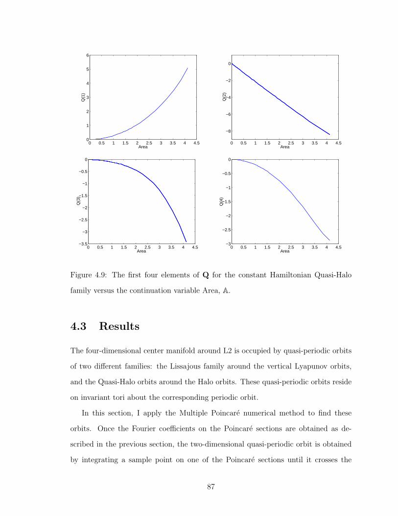
0 0.5 1 1.5 2 2.5 3 3.5 4 4.50
1
2
3
4
5
6
Area
Q(1
)
0 0.5 1 1.5 2 2.5 3 3.5 4 4.5
−8
−6
−4
−2
0
Area
Q(2
)
0 0.5 1 1.5 2 2.5 3 3.5 4 4.5−3.5
−3
−2.5
−2
−1.5
−1
−0.5
0
Area
Q(3
)
0 0.5 1 1.5 2 2.5 3 3.5 4 4.5−3
−2.5
−2
−1.5
−1
−0.5
0
Area
Q(4
)
Figure 4.9: The first four elements of Q for the constant Hamiltonian Quasi-Halo
family versus the continuation variable Area, A.
4.3 Results
The four-dimensional center manifold around L2 is occupied by quasi-periodic orbits
of two different families: the Lissajous family around the vertical Lyapunov orbits,
and the Quasi-Halo orbits around the Halo orbits. These quasi-periodic orbits reside
on invariant tori about the corresponding periodic orbit.
In this section, I apply the Multiple Poincare numerical method to find these
orbits. Once the Fourier coefficients on the Poincare sections are obtained as de-
scribed in the previous section, the two-dimensional quasi-periodic orbit is obtained
by integrating a sample point on one of the Poincare sections until it crosses the
87
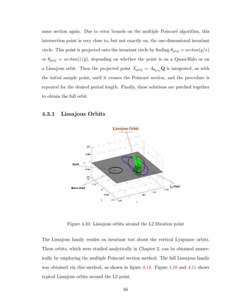
same section again. Due to error bounds on the multiple Poincare algorithm, this
intersection point is very close to, but not exactly on, the one-dimensional invariant
circle. This point is projected onto the invariant circle by finding θproj = arctan(y/x)
or θproj = arctan(z/y), depending on whether the point is on a Quasi-Halo or on
a Lissajous orbit. Then the projected point Xproj = AθprojQ is integrated, as with
the initial sample point, until it crosses the Poincare section, and the procedure is
repeated for the desired period length. Finally, these solutions are patched together
to obtain the full orbit.
4.3.1 Lissajous Orbits
Figure 4.10: Lissajous orbits around the L2 libration point
The Lissajous family resides on invariant tori about the vertical Lyapunov orbits.
These orbits, which were studied analytically in Chapter 2, can be obtained numer-
ically by employing the multiple Poincare section method. The full Lissajous family
was obtained via this method, as shown in figure 4.14. Figure 4.10 and 4.11 shows
typical Lissajous orbits around the L2 point.
88

1.008 1.0085 1.009 1.0095 1.01 1.0105 1.011−4
−3
−2
−1
0
1
2
3
4x 10
−3
X (AU)
Y (
AU
)
1.008 1.0085 1.009 1.0095 1.01 1.0105 1.011−8
−6
−4
−2
0
2
4
6
8x 10
−3
X (AU)
Z (
AU
)
−4 −2 0 2 4
x 10−3
−8
−6
−4
−2
0
2
4
6
8x 10
−3
Y (AU)
Z (
AU
)
1.0081.009
1.011.011
−4−2024−8
−6
−4
−2
0
2
4
6
8
X (AU)Y (AU x 10−3)
Z (
AU
x 1
0−3 )
Figure 4.11: Example of a Lissajous Orbit around L2
89

4.3.2 Quasi-Halo Orbits
Figure 4.12: Quasi-Halo orbits around the L2 libration point
The quasi-halo family reside on invariant tori about the halo orbits. These orbits
which were studied analytically in chapter 2 can be obtained numerically by employing
the multiple Poincare section method. The full Quasi-Halo family was obtained via
this method, as shown in figure 4.14. Figure 4.12 and 4.13 shows typical Quasi-Halo
orbits around the L2 point.
90
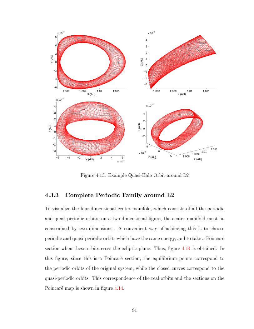
1.008 1.009 1.01 1.011−6
−4
−2
0
2
4
6x 10
−3
X (AU)
Y (
AU
)
1.008 1.009 1.01 1.011
−3
−2
−1
0
1
2
3
4
x 10−3
X (AU)
Z (
AU
)
−6 −4 −2 0 2 4 6
x 10−3
−3
−2
−1
0
1
2
3
4
x 10−3
Y (AU)
Z (
AU
)
1.0081.009
1.011.011
−5
0
5
x 10−3
−2
0
2
4
x 10−3
X (AU)Y (AU)
Z (
AU
)
Figure 4.13: Example Quasi-Halo Orbit around L2
4.3.3 Complete Periodic Family around L2
To visualize the four-dimensional center manifold, which consists of all the periodic
and quasi-periodic orbits, on a two-dimensional figure, the center manifold must be
constrained by two dimensions. A convenient way of achieving this is to choose
periodic and quasi-periodic orbits which have the same energy, and to take a Poincare
section when these orbits cross the ecliptic plane. Thus, figure 4.14 is obtained. In
this figure, since this is a Poincare section, the equilibrium points correspond to
the periodic orbits of the original system, while the closed curves correspond to the
quasi-periodic orbits. This correspondence of the real orbits and the sections on the
Poincare map is shown in figure 4.14.
91
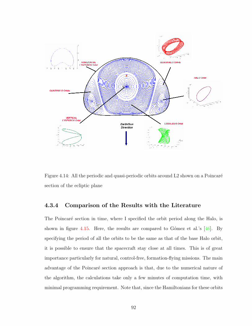
Figure 4.14: All the periodic and quasi-periodic orbits around L2 shown on a Poincare
section of the ecliptic plane
4.3.4 Comparison of the Results with the Literature
The Poincare section in time, where I specified the orbit period along the Halo, is
shown in figure 4.15. Here, the results are compared to Gomez et al.’s [46]. By
specifying the period of all the orbits to be the same as that of the base Halo orbit,
it is possible to ensure that the spacecraft stay close at all times. This is of great
importance particularly for natural, control-free, formation-flying missions. The main
advantage of the Poincare section approach is that, due to the numerical nature of
the algorithm, the calculations take only a few minutes of computation time, with
minimal programming requirement. Note that, since the Hamiltonians for these orbits
92
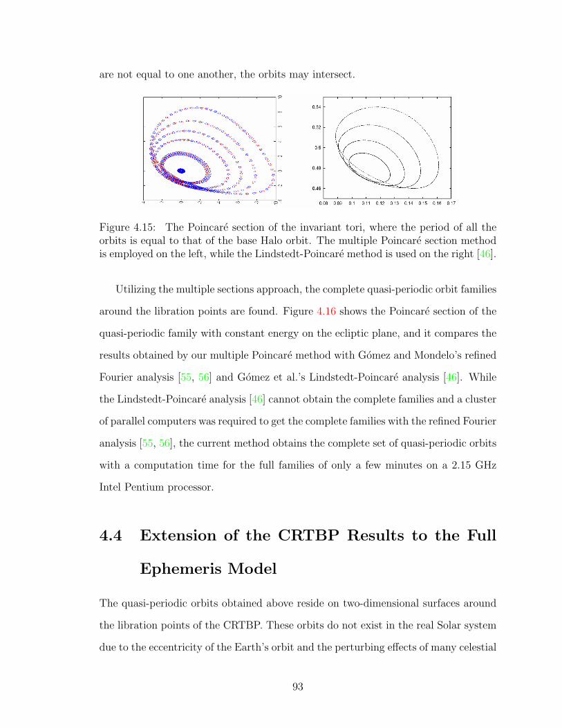
are not equal to one another, the orbits may intersect.
Figure 4.15: The Poincare section of the invariant tori, where the period of all theorbits is equal to that of the base Halo orbit. The multiple Poincare section methodis employed on the left, while the Lindstedt-Poincare method is used on the right [46].
Utilizing the multiple sections approach, the complete quasi-periodic orbit families
around the libration points are found. Figure 4.16 shows the Poincare section of the
quasi-periodic family with constant energy on the ecliptic plane, and it compares the
results obtained by our multiple Poincare method with Gomez and Mondelo’s refined
Fourier analysis [55, 56] and Gomez et al.’s Lindstedt-Poincare analysis [46]. While
the Lindstedt-Poincare analysis [46] cannot obtain the complete families and a cluster
of parallel computers was required to get the complete families with the refined Fourier
analysis [55, 56], the current method obtains the complete set of quasi-periodic orbits
with a computation time for the full families of only a few minutes on a 2.15 GHz
Intel Pentium processor.
4.4 Extension of the CRTBP Results to the Full
Ephemeris Model
The quasi-periodic orbits obtained above reside on two-dimensional surfaces around
the libration points of the CRTBP. These orbits do not exist in the real Solar system
due to the eccentricity of the Earth’s orbit and the perturbing effects of many celestial
93

Figure 4.16: The Poincare section of the complete quasi-periodic family around L2with energy that is equivalent to the 500,000 km-sized halo orbit on the ecliptic plane(on the left). Similar results from Gomez & Mondelo [55, 56] (in the middle) andGomez et al. [46] (on the right).
bodies. Nevertheless, since the CRTBP is a good first-order approximation to the real
Solar System dynamics, there are orbits in the Solar System that have very similar
shapes and properties to the orbits found in the simplified problem. The aim of this
chapter is to find these orbits.
I take the real Solar System dynamics to be the point-mass gravitational inter-
actions of the major Solar system bodies given at each time-instant with the JPL
DE-406, which is the latest version of the JPL Solar System Ephemeris [57]. It spec-
ifies the past and future positions of the Sun, Moon, and nine planets (Pluto is still
defined as a planet in this ephemeris) in three-dimensional space. The ephemeris gives
the Chebyshev polynomial coefficients corresponding to the J2000 standard epoch po-
sitions of these Solar bodies [57, 58]. In the calculations to follow, deviation from the
spherical symmetry of the bodies such as oblateness is not taken into account. Since
the specifications of the spacecraft that will be placed in these orbits are not known,
neither are drag and solar pressure included in the study. However, note that for a
spherical spacecraft, the effect of solar pressure can easily be included without any
additional force terms, by only reducing the effective mass of the Sun. This is the case
because both the gravitation and the solar pressure forces are inversely proportional
94
to distance square (i.e. F ∝ 1r2 ), only differing by a constant.
The aim is to find real solar trajectories that have the same characteristics as
the quasi-periodic orbits obtained in this chapter. Thus, the algorithm first takes
the orbits in the CRTBP and converts them from the synodical frame to the so-
lar frame. For astronomically simplified models, better results are obtained when
the Earth/Moon system is treated as a single planet with the center-of-mass at the
Earth/Moon Barycenter, than when the effect of the Moon is ignored in the model.
I employ the usual synodical frame, which has its center at the center-of-mass
of the Sun-Earth/Moon Barycenter system, to map the CRTBP results to the full
solar model, and I find that the large distance between the Sun and the spacecraft
trajectory leads to undesirable behavior. Multiplying small errors with this large
distance leads to non-convergent transfers. Thus, I move the position of the axis
center from the usual definition, which is the center-of-mass of the Sun-Earth/Moon
Barycenter system, to the Earth/Moon Barycenter. In order to map the synodical
coordinates to solar coordinates, the following steps are taken.
In what follows, subscripts cm, syn, sun, em, and e/s refer, respectively, to the center-
of-mass synodical frame, the Sun, the Earth/Moon Barycenter, and the Earth/Moon
Barycenter with respect to the Sun. Superscripts R and I refer to the rotating and the
inertial coordinates. r and v are the position and velocity components of the space-
craft. Finally, R and V are the position and velocity components of the solar system
bodies with respect to the solar system center-of-mass, unless specified otherwise.
1. First, the position and velocities of the Sun, the Earth/Moon Barycenter, and
their relative distances are obtained from DE-406:
~Re/s = ~Rem − ~Rsun . (4.59)
95

2. The position, velocity and rotation rate of the rotating frame are calculated:
~Rcm = ~Rem ,
~Vcm = ~Vem ,
~ωsyn =~Rs/e × ~Rs/e
|~Rs/e|2. (4.60)
3. (1 − µ) is subtracted from the x-coordinates of the synodical frame elements,
and the synodical elements are multiplied with the length and time scale to
redimensionize the coordinates:
~rRsyn = ||~Rs/e||
(~rR
syn − 1− µ, 0, 0 T),
~vRsyn = ||~Rs/e|| ||~ωsyn|| ~vR
syn . (4.61)
4. The rotation matrix is obtained from the synodical frame to inertial frame:
R = [ e1 e2 e3 ] , (4.62)
where
e1 =~Rs/e
||~Rs/e||, e3 =
~ωsyn
||~ωsyn||, and e2 =
e3 × e1||e3 × e1||
. (4.63)
5. The synodical coordinates are expressed in inertial frame coordinates:
~rIsyn = R~rR
syn ,
~vIsyn = R ~vR
syn . (4.64)
6. Finally, the inertial position, ~rIsolar, and velocity, ~rI
solar, of the spacecraft are
96

found with respect to the solar center-of-mass:
~rIsolar = ~rI
syn + ~Rcm ,
~vIsolar = ~vI
syn + ~ωsyn ×~rIsyn + ~Vcm . (4.65)
Once the position and velocities are mapped to solar system coordinates, I take
these orbits as initial guesses, and find the natural orbits in the full ephemeris model
that stay close to them. My approach to this problem was to take an orbit for a
specified time interval, which would be the time frame of the mission, and to feed this
guess to the collocation algorithm. However, this time, I ran the algorithm without
boundary conditions (see section 3.1.1 for details of the implementation). Thus,
without any constraints, I look for an orbit that satisfies the full Solar System ODE,
starting with the initial guess obtained from the CRTBP. The result is a natural orbit
of the Solar System which is very close in shape and characteristics to the CRTBP
orbit.
The main advantage of this approach is that all the available information, i.e.,
the full guess for the orbit, is used. This is helpful because the Halo and Quasi-Halo
orbits around L2 are unstable, and long-term integration with bad initial guesses
might lead to trajectories that diverge from the original orbit. Thus, I employ a
collocation algorithm, which is a robust boundary value problem-solving technique.
Finally, for visualization purposes, the results in the solar coordinates are con-
verted back to the synodical frame by applying the algorithm backwards. Figures
4.17, 4.18, and 4.19 show the results for three different types of orbits - Halo, Quasi-
Halo and Lissajous orbits - around the Sun-Earth L2 point, transferred to the JPL
DE-406 model.
The collocation algorithm performs robustly around the Sun-Earth L2 point where
the missions of our interest will be located. I also implemented the multiple shoot-
97
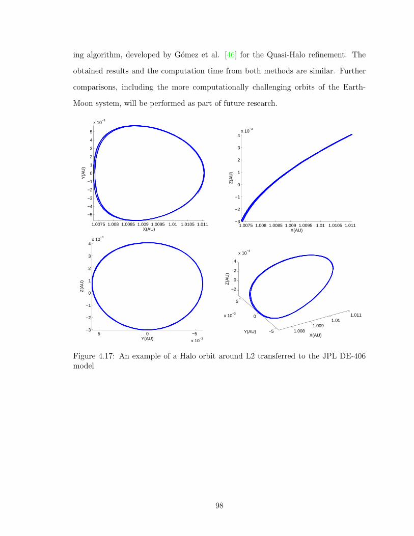
ing algorithm, developed by Gomez et al. [46] for the Quasi-Halo refinement. The
obtained results and the computation time from both methods are similar. Further
comparisons, including the more computationally challenging orbits of the Earth-
Moon system, will be performed as part of future research.
1.0075 1.008 1.0085 1.009 1.0095 1.01 1.0105 1.011
−5
−4
−3
−2
−1
0
1
2
3
4
5
x 10−3
X(AU)
Y(A
U)
1.0075 1.008 1.0085 1.009 1.0095 1.01 1.0105 1.011−3
−2
−1
0
1
2
3
4x 10
−3
X(AU)Z
(AU
)
−505
x 10−3
−3
−2
−1
0
1
2
3
4x 10
−3
Y(AU)
Z(A
U)
1.0081.009
1.011.011
−5
0
5
x 10−3
−2
0
2
4
x 10−3
X(AU)Y(AU)
Z(A
U)
Figure 4.17: An example of a Halo orbit around L2 transferred to the JPL DE-406model
98
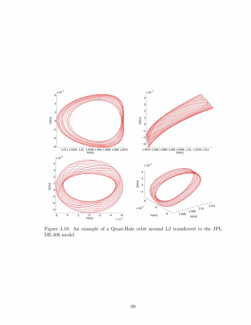
1.00751.0081.00851.0091.00951.011.01051.011−6
−4
−2
0
2
4
6x 10
−3
X(AU)
Y(A
U)
1.0075 1.008 1.0085 1.009 1.0095 1.01 1.0105 1.011
−3
−2
−1
0
1
2
3
4
x 10−3
X(AU)
Z(A
U)
−6−4−20246
x 10−3
−3
−2
−1
0
1
2
3
4
x 10−3
Y(AU)
Z(A
U)
1.0081.009
1.011.011
−5
0
5
x 10−3
−2
0
2
4
x 10−3
X(AU)Y(AU)
Z(A
U)
Figure 4.18: An example of a Quasi-Halo orbit around L2 transferred to the JPLDE-406 model
99
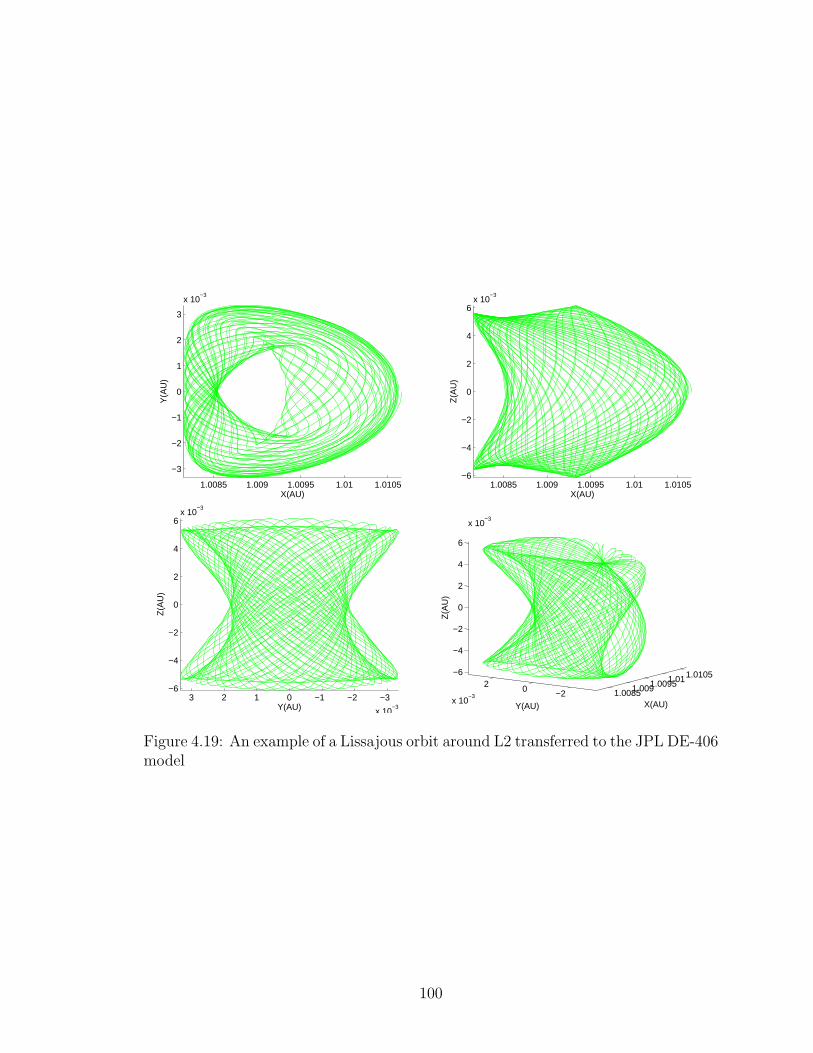
1.0085 1.009 1.0095 1.01 1.0105
−3
−2
−1
0
1
2
3
x 10−3
X(AU)
Y(A
U)
1.0085 1.009 1.0095 1.01 1.0105−6
−4
−2
0
2
4
6x 10
−3
X(AU)
Z(A
U)
−3−2−10123
x 10−3
−6
−4
−2
0
2
4
6x 10
−3
Y(AU)
Z(A
U)
1.00851.0091.00951.011.0105
−202
x 10−3
−6
−4
−2
0
2
4
6
x 10−3
X(AU)Y(AU)
Z(A
U)
Figure 4.19: An example of a Lissajous orbit around L2 transferred to the JPL DE-406model
100
Chapter 5
Finding the Optimal Trajectories
101
The control problem can be separated into two parts; first, the line-of-sight (LOS)
control of the formation during imaging, and second, the trajectory control for ma-
neuvering the occulter from one star LOS to another between imaging sessions, i.e.,
the realignment maneuver. Here, I focus on the latter, since the realignment dom-
inates the Delta-V budget. In this chapter, I find the optimal trajectories for the
realignment processes. Although this is not the main aim of this chapter, I also
solved for the optimal trajectories from Earth to Halo orbits as a sample problem for
the control algorithms that were developed, and to give an idea about the transfer
trajectories.
5.1 Different Optimal Control Approaches
During the imaging of a given planetary system, the telescope and the occulter must
be aligned to the LOS of the star position. Thus, the inertial velocities of the telescope
and the occulter should be the same. In addition, the optics of the diffraction pattern
are such that the telescope will most probably be designed for a prespecified constant
occulter-telescope separation. Thus, based on this optical constraint, the distance
between the occulter and the telescope should be roughly the same for all observations.
This fixes the position of the occulter to be on a sphere around the telescope. The
realignment problem then becomes one of finding an optimal trajectory between two
two-dimensional surfaces, as shown in figure 5.1. I examine six optimization strategies
for the realignment. Depending on the type of thruster the mission uses, either
continuous or discrete control might be needed. Since the most probable devices
are Hall-type thrusters, where we have access to continuous, low magnitude thrust
throughout the trajectory, I studied five continuous thrust methods (and one discrete
one). For all the control algorithms developed in this chapter, I assume that the
there is a single thruster that can be instantaneously thrusted towards any direction
102
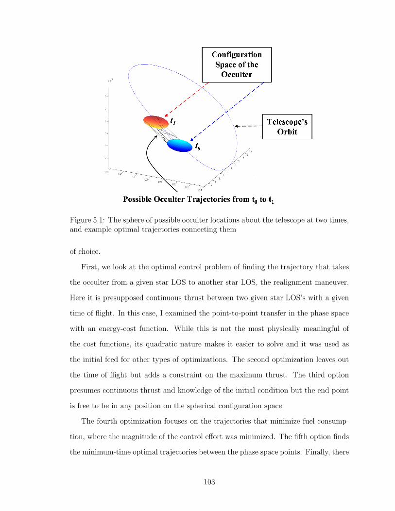
Figure 5.1: The sphere of possible occulter locations about the telescope at two times,and example optimal trajectories connecting them
of choice.
First, we look at the optimal control problem of finding the trajectory that takes
the occulter from a given star LOS to another star LOS, the realignment maneuver.
Here it is presupposed continuous thrust between two given star LOS’s with a given
time of flight. In this case, I examined the point-to-point transfer in the phase space
with an energy-cost function. While this is not the most physically meaningful of
the cost functions, its quadratic nature makes it easier to solve and it was used as
the initial feed for other types of optimizations. The second optimization leaves out
the time of flight but adds a constraint on the maximum thrust. The third option
presumes continuous thrust and knowledge of the initial condition but the end point
is free to be in any position on the spherical configuration space.
The fourth optimization focuses on the trajectories that minimize fuel consump-
tion, where the magnitude of the control effort was minimized. The fifth option finds
the minimum-time optimal trajectories between the phase space points. Finally, there
103

is the discrete control consisting of two impulsive Delta-V maneuvers, one at the be-
ginning and one at the end of the trajectory.
In the following sections, I go over these six different optimization strategies,
and I discuss the approaches taken to solve the optimal control problem that arises
from these different assumptions. Before going any further, I first review the general
optimal control problem.
The stars to be observed were taken from the list with the most suitable 100 stars
for the TPF-C mission [59]. I then used the astrometrical data from the Hipparcos
astronomical catalog [60]. I employed the NOVAS routines developed by Kaplan [61]
to convert and update the exact star locations of the target stars relative to the Solar
system, starting from 1 January 2010, the mission start day of my choice. For high-
fidelity applications, I developed the capability to use the full nonlinear solar system
model based on the JPL DE-406 ephemeris [57] for differential equations. However,
in the analysis to follow, the CRTBP simplified model is used for the dynamical
model, and a uniformly rotating star model is employed for the star locations for
faster calculations.
For ease of comparison, all the missions scenarios discussed from here on assume
a base Halo orbit around L2 with an out-of-plane amplitude of 500,000 km.
5.1.1 The Euler-Lagrange Formulation of the Optimal Con-
trol Problem (Indirect Method)
The Euler-Lagrange method, otherwise known as the adjoint method, employs the
variational calculus to find the optimal control of a differential system. Here I only
outline the methodology; for details see Stengel [62] and Bryson & Ho [63]. I wish to
find a trajectory, x(t), and control, u(t), that minimizes the cost function, J , in the
104
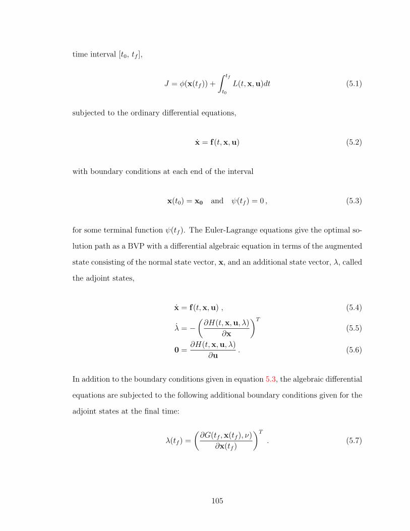
time interval [t0, tf ],
J = φ(x(tf )) +
∫ tf
t0
L(t,x,u)dt (5.1)
subjected to the ordinary differential equations,
x = f(t,x,u) (5.2)
with boundary conditions at each end of the interval
x(t0) = x0 and ψ(tf ) = 0 , (5.3)
for some terminal function ψ(tf ). The Euler-Lagrange equations give the optimal so-
lution path as a BVP with a differential algebraic equation in terms of the augmented
state consisting of the normal state vector, x, and an additional state vector, λ, called
the adjoint states,
x = f(t,x,u) , (5.4)
λ = −(∂H(t,x,u, λ)
∂x
)T
(5.5)
0 =∂H(t,x,u, λ)
∂u. (5.6)
In addition to the boundary conditions given in equation 5.3, the algebraic differential
equations are subjected to the following additional boundary conditions given for the
adjoint states at the final time:
λ(tf ) =
(∂G(tf ,x(tf ), ν)
∂x(tf )
)T
. (5.7)
105
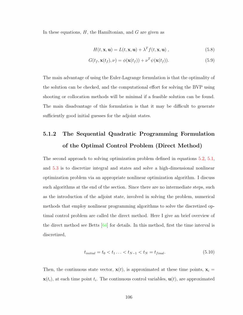
In these equations, H, the Hamiltonian, and G are given as
H(t,x,u) = L(t,x,u) + λTf(t,x,u) , (5.8)
G(tf ,x(tf ), ν) = φ(x(tf )) + νTψ(x(tf )). (5.9)
The main advantage of using the Euler-Lagrange formulation is that the optimality of
the solution can be checked, and the computational effort for solving the BVP using
shooting or collocation methods will be minimal if a feasible solution can be found.
The main disadvantage of this formulation is that it may be difficult to generate
sufficiently good initial guesses for the adjoint states.
5.1.2 The Sequential Quadratic Programming Formulation
of the Optimal Control Problem (Direct Method)
The second approach to solving optimization problem defined in equations 5.2, 5.1,
and 5.3 is to discretize integral and states and solve a high-dimensional nonlinear
optimization problem via an appropriate nonlinear optimization algorithm. I discuss
such algorithms at the end of the section. Since there are no intermediate steps, such
as the introduction of the adjoint state, involved in solving the problem, numerical
methods that employ nonlinear programming algorithms to solve the discretized op-
timal control problem are called the direct method. Here I give an brief overview of
the direct method see Betts [64] for details. In this method, first the time interval is
discretized,
tinitial = t0 < t1 . . . < tN−1 < tN = tfinal. (5.10)
Then, the continuous state vector, x(t), is approximated at these time points, xi =
x(ti), at each time point ti. The continuous control variables, u(t), are approximated
106
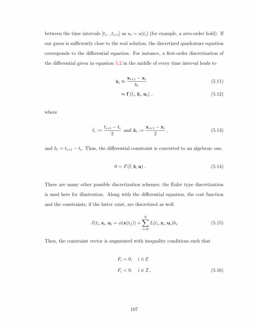
between the time intervals [ti, , ti+1] as ui = u(ti) (for example, a zero-order hold). If
our guess is sufficiently close to the real solution, the discretized quadrature equation
corresponds to the differential equation. For instance, a first-order discretization of
the differential given in equation 5.2 in the middle of every time interval leads to
xi ≈xi+1 − xi
hi
(5.11)
≈ f (ti, xi,ui) , (5.12)
where
ti :=ti+1 − ti
2and xi :=
xi+1 − xi
2, (5.13)
and hi = ti+1 − ti. Thus, the differential constraint is converted to an algebraic one,
0 = F (t, x,u) . (5.14)
There are many other possible discretization schemes; the Euler type discretization
is used here for illustration. Along with the differential equation, the cost function
and the constraints, if the latter exist, are discretized as well.
J(ti,xi,ui = φ(x(tf )) +N∑
i=0
L(ti,xi,ui)hi (5.15)
Then, the constraint vector is augmented with inequality conditions such that
Fi = 0, i ∈ E
Fi < 0, i ∈ I , (5.16)
107
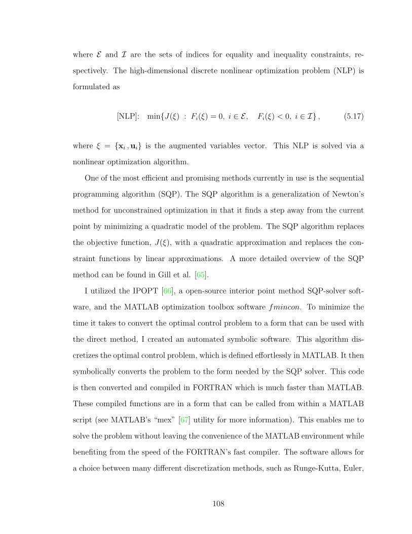
where E and I are the sets of indices for equality and inequality constraints, re-
spectively. The high-dimensional discrete nonlinear optimization problem (NLP) is
formulated as
[NLP]: minJ(ξ) : Fi(ξ) = 0, i ∈ E , Fi(ξ) < 0, i ∈ I , (5.17)
where ξ = xi ,ui is the augmented variables vector. This NLP is solved via a
nonlinear optimization algorithm.
One of the most efficient and promising methods currently in use is the sequential
programming algorithm (SQP). The SQP algorithm is a generalization of Newton’s
method for unconstrained optimization in that it finds a step away from the current
point by minimizing a quadratic model of the problem. The SQP algorithm replaces
the objective function, J(ξ), with a quadratic approximation and replaces the con-
straint functions by linear approximations. A more detailed overview of the SQP
method can be found in Gill et al. [65].
I utilized the IPOPT [66], a open-source interior point method SQP-solver soft-
ware, and the MATLAB optimization toolbox software fmincon. To minimize the
time it takes to convert the optimal control problem to a form that can be used with
the direct method, I created an automated symbolic software. This algorithm dis-
cretizes the optimal control problem, which is defined effortlessly in MATLAB. It then
symbolically converts the problem to the form needed by the SQP solver. This code
is then converted and compiled in FORTRAN which is much faster than MATLAB.
These compiled functions are in a form that can be called from within a MATLAB
script (see MATLAB’s “mex” [67] utility for more information). This enables me to
solve the problem without leaving the convenience of the MATLAB environment while
benefiting from the speed of the FORTRAN’s fast compiler. The software allows for
a choice between many different discretization methods, such as Runge-Kutta, Euler,
108

and trapezoidal, in order to suit the needs of the specific problem. I hope to make
this software available for the public soon.
5.2 Unconstrained Minimum Energy Optimization
In this approach, I assume that the control variable is the acceleration of the spacecraft
due to the force applied by the thrusters throughout its trajectory, u = (d2xdt2
)thruster.
Then, the effect of the control can be added to the normal control-free Newtonian
equations such that
x = fctr(t,x,u) , (5.18)
where
fctr(t,x,u) = f(t,x) + 0, 0, 0, ux, uy, uz T , (5.19)
and where the control vector, u, is defined as u = ux, uy, uz T . My aim is to
minimize the control effort given these differential equations of motion. In this section,
I use a cost function of the quadratic form,
J =
∫ tf
t0
1
2u · u dt . (5.20)
Here, I use the notation, ·, for the dot product of vectors. The Hamiltonian for this
optimal control problem is
H(t,x, λ,u) =1
2u · u + λT f(t,x) + pTu , (5.21)
109
where I use the intermediate variable, p, which is the last three elements of the adjoint
vector:
p = λ4, λ5, λ6 T . (5.22)
In this section, I consider the point-to-point optimal control, where both the initial
and final states are fixed a priori.
ψ(tf ) = x(tf )− xf = 0 (5.23)
Solving the optimality condition,
0 =∂H(t,x, λ,u)
∂u(5.24)
I obtain,
u = −p . (5.25)
Substituting for u in the Euler-Lagrange equations, I obtain a 12-degree ODE in
terms of the state and adjoint state only:
x = f(t,x, λ) ,
λ = −(∂f(t,x)
∂x
)T
λ , (5.26)
with twelve boundary conditions
x(t0)− x0
x(tf )− xf
= 0 . (5.27)
110
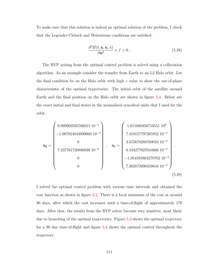
To make sure that this solution is indeed an optimal solution of the problem, I check
that the Legendre-Clebsch and Weierstrass conditions are satisfied:
∂2H(t,x,u, λ)
∂u2= I > 0 . (5.28)
The BVP arising from the optimal control problem is solved using a collocation
algorithm. As an example consider the transfer from Earth to an L2 Halo orbit. Let
the final condition be on the Halo orbit with high z value to show the out-of-plane
characteristic of the optimal trajectories. The initial orbit of the satellite around
Earth and the final position on the Halo orbit are shown in figure 5.3. Below are
the exact initial and final states in the normalized synodical units that I used for the
orbit.
x0 =
9.999969595766015 10−1
−1.007824043999068 10−3
0
7.237761726886938 10−2
0
0
, xf =
1.011080356710551 100
7.419127797265952 10−4
3.655679288769010 10−3
6.534277927644666 10−4
−1.054583863270762 10−2
7.362873998458644 10−4
.
(5.29)
I solved the optimal control problem with various time intervals and obtained the
cost function as shown in figure 5.2. There is a local minimum of the cost at around
90 days, after which the cost increases until a time-of-flight of approximately 170
days. After that, the results from the BVP solver become very sensitive, most likely
due to branching of the optimal trajectories. Figure 5.3 shows the optimal trajectory
for a 90 day time-of-flight and figure 5.4 shows the optimal control throughout the
trajectory.
111
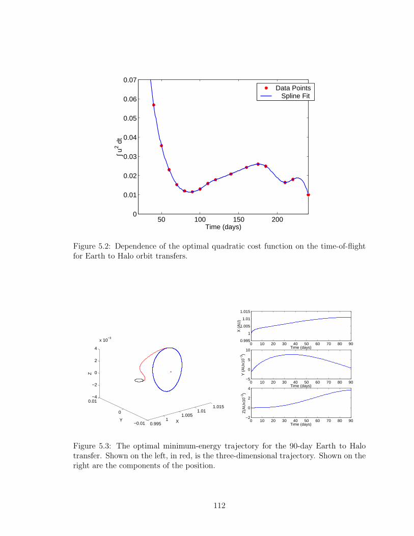
50 100 150 2000
0.01
0.02
0.03
0.04
0.05
0.06
0.07
Time (days)
∫ u2 d
t
Data Points Spline Fit
Figure 5.2: Dependence of the optimal quadratic cost function on the time-of-flightfor Earth to Halo orbit transfers.
0.9951
1.0051.01
1.015
−0.01
0
0.01−4
−2
0
2
4
x 10−3
XY
Z
0 10 20 30 40 50 60 70 80 900.995
1
1.005
1.01
1.015
Time (days)
X (
AU
)
0 10 20 30 40 50 60 70 80 90−5
0
5
10
Time (days)
Y (
AU
x10−
3 )
0 10 20 30 40 50 60 70 80 90−2
0
2
4
Time (days)
Z(A
Ux1
0−3 )
Figure 5.3: The optimal minimum-energy trajectory for the 90-day Earth to Halotransfer. Shown on the left, in red, is the three-dimensional trajectory. Shown on theright are the components of the position.
112
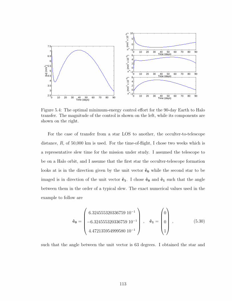
0 10 20 30 40 50 60 70 80 902.5
3
3.5
4
4.5
5
5.5
6
6.5
7
7.5
Time (days)
||u||
(m/s
2 )
0 10 20 30 40 50 60 70 80 90−5
0
5
10
Time (days)
u x (m
/s2 x
10−
5 )
0 10 20 30 40 50 60 70 80 90−2
0
2
4
6
Time (days)
u y (m
/s2 x
10−
5 )
0 10 20 30 40 50 60 70 80 90−2
0
2
4
6
Time (days)
u z (m
/s2 x
10−
5 )
Figure 5.4: The optimal minimum-energy control effort for the 90-day Earth to Halotransfer. The magnitude of the control is shown on the left, while its components areshown on the right.
For the case of transfer from a star LOS to another, the occulter-to-telescope
distance, R, of 50,000 km is used. For the time-of-flight, I chose two weeks which is
a representative slew time for the mission under study. I assumed the telescope to
be on a Halo orbit, and I assume that the first star the occulter-telescope formation
looks at is in the direction given by the unit vector e0 while the second star to be
imaged is in direction of the unit vector e1. I chose e0 and e1 such that the angle
between them in the order of a typical slew. The exact numerical values used in the
example to follow are
e0 =
6.324555320336759 10−1
−6.324555320336759 10−1
4.472135954999580 10−1
, e1 =
0
0
1
, (5.30)
such that the angle between the unit vector is 63 degrees. I obtained the star and
113
end positions the occulters from the unit vectors as
rocc = rtel +R e , (5.31)
where rocc and rtel are the position of the occulter and the telescope in the synodical
frame, respectively. I obtained the velocities based on the requirement that the inertial
velocities of both the telescope and the occulter be the same,
vocc = vtel + ω ×R e , (5.32)
where vocc and vtel are the velocity of the occulter and the telescope, respectively,
and ω = 0, 0, 1T is the angular velocity of the CTRBP. Thus, the numerical values
in the normalized synodical units for the BVP algorithm are
x0 =
1.008708480181499 100
5.219658053604695 10−3
1.494719120781122 10−4
3.123278717913480 10−3
2.077725728577118 10−3
6.483432393011172 10−3
, xf =
1.009397510830226 100
5.341370714348193 10−3
1.843136365772625 10−3
3.951895067977367 10−3
−2.937081366176431 10−3
5.838803068471303 10−3
. (5.33)
Figure 5.5 shows the optimal trajectory of the occulter relative to the telescope on
the Halo orbit. Figure 5.6 shows the optimal control throughout the trajectory.
5.3 Constrained Minimum Energy Optimization
Next, I add an inequality constraint on the control to the minimum energy problem.
The magnitude of the control vector, |u|, must be less than a specified limit, umax,
such that |u| < umax. The augmented Hamiltonian for the optimal control problem
114
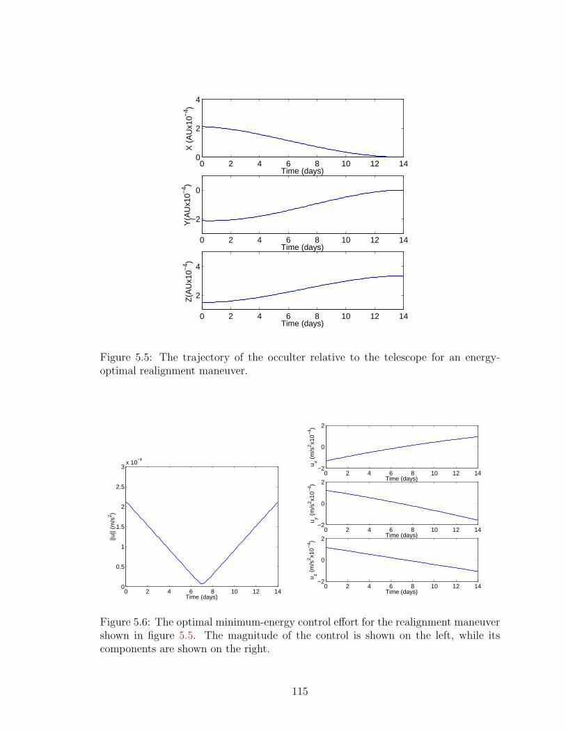
0 2 4 6 8 10 12 140
2
4
Time (days)
X (
AU
x10−
4 )
0 2 4 6 8 10 12 14
−2
0
Time (days)
Y(A
Ux1
0−4 )
0 2 4 6 8 10 12 14
2
4
Time (days)
Z(A
Ux1
0−4 )
Figure 5.5: The trajectory of the occulter relative to the telescope for an energy-optimal realignment maneuver.
0 2 4 6 8 10 12 140
0.5
1
1.5
2
2.5
3x 10
−4
Time (days)
||u||
(m/s
2 )
0 2 4 6 8 10 12 14−2
0
2
Time (days)
u x (m
/s2 x1
0−4 )
0 2 4 6 8 10 12 14−2
0
2
Time (days)
u y (m
/s2 x1
0−4 )
0 2 4 6 8 10 12 14−2
0
2
Time (days)
u z (m
/s2 x1
0−4 )
Figure 5.6: The optimal minimum-energy control effort for the realignment maneuvershown in figure 5.5. The magnitude of the control is shown on the left, while itscomponents are shown on the right.
115
can be written as
Haug(t,x, λ,u) =1
2u · u + λT f(t,x) + pTu + µeffceff (u)
µeff = 0 if ceff (u) < 0
µeff > 0 if ceff (u) = 0 ,
(5.34)
where ceff (u) is the inequality constraint function effective on the boundary,
ceff (u) = u · u− u2max 6 0 , (5.35)
and µeff is the corresponding Lagrange multiplier.
Since ceff is only a function of u, the adjoint differential equations are not altered.
However, the condition for control optimality becomes
0 =∂H
∂u
T
=
u + p, ceff < 0
u + p + 2µeffu, ceff = 0 .
(5.36)
Solving the first part of the equation gives u = −p, as before. The second part asks
that the following two equations be satisfied:
u = − p
1 + 2µeff
and |u| = umax , (5.37)
which are solved to give
u = ±umaxp
|p|. (5.38)
In order to decide which sign the control should take, I use the Pontryagin’s Minimum
Principle (See Stengel for details [62]), which states that the optimal control, u∗, in
116
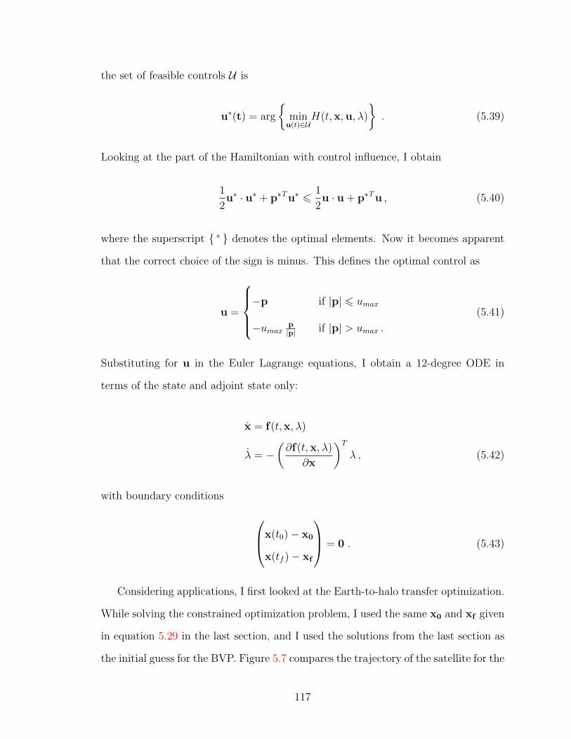
the set of feasible controls U is
u∗(t) = arg
min
u(t)∈UH(t,x,u, λ)
. (5.39)
Looking at the part of the Hamiltonian with control influence, I obtain
1
2u∗ · u∗ + p∗Tu∗ 6
1
2u · u + p∗Tu , (5.40)
where the superscript ∗ denotes the optimal elements. Now it becomes apparent
that the correct choice of the sign is minus. This defines the optimal control as
u =
−p if |p| 6 umax
−umaxp|p| if |p| > umax .
(5.41)
Substituting for u in the Euler Lagrange equations, I obtain a 12-degree ODE in
terms of the state and adjoint state only:
x = f(t,x, λ)
λ = −(∂f(t,x, λ)
∂x
)T
λ , (5.42)
with boundary conditions
x(t0)− x0
x(tf )− xf
= 0 . (5.43)
Considering applications, I first looked at the Earth-to-halo transfer optimization.
While solving the constrained optimization problem, I used the same x0 and xf given
in equation 5.29 in the last section, and I used the solutions from the last section as
the initial guess for the BVP. Figure 5.7 compares the trajectory of the satellite for the
117
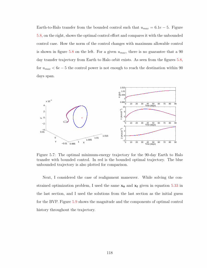
Earth-to-Halo transfer from the bounded control such that umax = 6.1e − 5. Figure
5.8, on the right, shows the optimal control effort and compares it with the unbounded
control case. How the norm of the control changes with maximum allowable control
is shown in figure 5.8 on the left. For a given umax, there is no guarantee that a 90
day transfer trajectory from Earth to Halo orbit exists. As seen from the figures 5.8,
for umax < 6e− 5 the control power is not enough to reach the destination within 90
days span.
0.9951
1.0051.01
1.015
−0.01
0
0.01−4
−2
0
2
4
x 10−3
XY
Z
0 10 20 30 40 50 60 70 80 900.995
1
1.005
1.01
1.015
Time (days)
X (
AU
)
0 10 20 30 40 50 60 70 80 90−5
0
5
10
Time (days)
Y (
AU
x10−
3 )
0 10 20 30 40 50 60 70 80 90−2
0
2
4
Time (days)
Z (
AU
x10−
3 )
Figure 5.7: The optimal minimum-energy trajectory for the 90-day Earth to Halotransfer with bounded control. In red is the bounded optimal trajectory. The blueunbounded trajectory is also plotted for comparison.
Next, I considered the case of realignment maneuver. While solving the con-
strained optimization problem, I used the same x0 and xf given in equation 5.33 in
the last section, and I used the solutions from the last section as the initial guess
for the BVP. Figure 5.9 shows the magnitude and the components of optimal control
history throughout the trajectory.
118

0 10 20 30 40 50 60 70 80 902.5
3
3.5
4
4.5
5
5.5
6
6.5
7
7.5
Time (days)
||u||
(m/s
2 x10−
5 )
0 10 20 30 40 50 60 70 80 90−5
0
5
10
Time (days)
u x (m
/sx1
0−5 )
0 10 20 30 40 50 60 70 80 90−2
0
2
4
6
Time (days)
u y (m
/sx1
0−5 )
0 10 20 30 40 50 60 70 80 90−2
0
2
4
6
Time (days)
u z (m
/sx1
0−5 )
Figure 5.8: The optimal minimum-energy control effort for the 90-day Earth to Halotransfer with varying bounds on control. The effect of the varying bounds on themagnitude of the control effort is show on the left. The components of the controleffort are show on the right; red for a bounded case and blue for the unbounded one.
0 2 4 6 8 10 12 140
0.2
0.4
0.6
0.8
1
1.2
1.4
1.6
1.8x 10
−4
Time (days)
||u||
(m/s
2 )
0 2 4 6 8 10 12 14−1
−0.5
0
0.5
1
Time (days)
u x (m
/s2 x1
0−4 )
0 2 4 6 8 10 12 14−2
0
2
Time (days)
u y (m
/s2 x1
0−4 )
0 2 4 6 8 10 12 14−1
−0.5
0
0.5
1
Time (days)
u z (m
/s2 x1
0−4 )
Figure 5.9: An optimal minimum-energy control effort for the realignment maneuver.The magnitude of the control is shown on the left, while its components are shownon the right.
119
5.4 Free-End Condition Optimization
The third optimization presumes continuous thrust and knowledge of the initial con-
dition and leaves open the end point on the spherical configuration space at tf . In
this case, the initial state of the occulter, x(t0) = x0, is known at t = t0, and I seek
to find the target occulter state, x(tf ), at time tf , that minimizes the energy cost
function. Thus, the end time is fixed while the end position is free to change. Due
to the optical requirements that were discussed previously, this final position, x(tf ),
resides on the two-dimensional possible occulter locations at a given final time t = tf .
The Lagrangian and the differential equations are the same as before:
J =
∫ tf
t0
1
2u · u dt . (5.44)
The same Hamiltonian as before is also used:
H =1
2u · u + λT f(x) + pTu , (5.45)
but instead of the six-dimensional equality constant, x(tf ) = xf , at the end of the
interval, now there are only four conditions. The first of these constraints is that the
distance between the occulter and the telescope at the final time must be equal to
the predefined radius, R. The other three are that the inertial velocity vector of the
occulter and the telescope must be the same in order to be able to lock on a target
star. Noting that the inertial velocity is
v= = v< + ω × r , (5.46)
120
where ω = 0, 0, 1T , the final time constraint vector becomes
ψ(tf ) =
(x(tf )− xh(tf ))2 + (y(tf )− yh(tf ))
2 + (z(tf )− zh(tf ))2 −R2
x(tf )− y(tf )− (xh(tf )− yh(tf ))
y(tf ) + x(tf )− (yh(tf ) + xh(tf ))
z(tf )− zh(tf )
= 0 .
(5.47)
This four-dimensional condition does not change the differential equation for x and
λ, but the final condition for the adjoint variables becomes
λ(tf ) =
(∂G(tf ,xf , ν)
∂x(tf )
)T
=
ν1(x(tf )− xh(tf )) + ν3
ν1(y(tf )− yh(tf ))− ν2
ν1(z(tf )− zh(tf )
ν2
ν3
ν4
, (5.48)
where the components of ν, the constant Lagrange multiplier vector corresponding
to the end constraints, are given as ν = ν1, ν2, ν3, ν4. Eliminating the elements of
ν, these six equations can be turned into two constraints in term of λ(tf ):
ψadd(tf ) =
−λ1(tf ) + λ3(tf )x(tf )−xh(tf )
z(tf )−zh(tf )+ λ5
−λ2(tf ) + λ3(tf )y(tf )−yh(tf )
z(tf )−zh(tf )− λ4
. (5.49)
With the addition of the four ψ(tf ) constraints given in equation 5.47 on the final time
and the six initial conditions, x(t0) = x0, I obtain the twelve boundary conditions
121
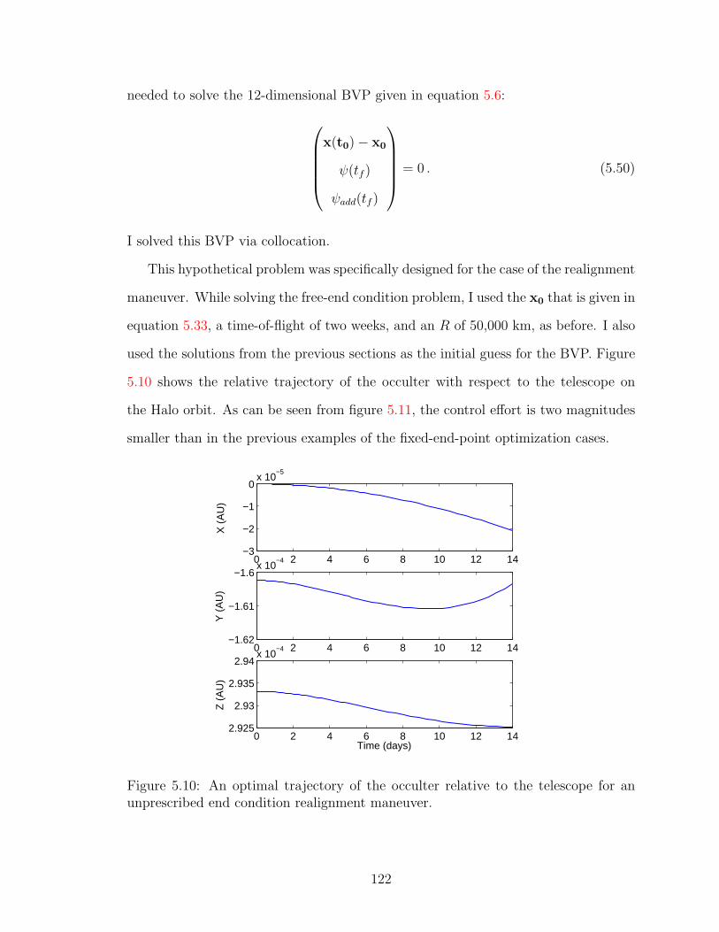
needed to solve the 12-dimensional BVP given in equation 5.6:
x(t0)− x0
ψ(tf )
ψadd(tf )
= 0 . (5.50)
I solved this BVP via collocation.
This hypothetical problem was specifically designed for the case of the realignment
maneuver. While solving the free-end condition problem, I used the x0 that is given in
equation 5.33, a time-of-flight of two weeks, and an R of 50,000 km, as before. I also
used the solutions from the previous sections as the initial guess for the BVP. Figure
5.10 shows the relative trajectory of the occulter with respect to the telescope on
the Halo orbit. As can be seen from figure 5.11, the control effort is two magnitudes
smaller than in the previous examples of the fixed-end-point optimization cases.
0 2 4 6 8 10 12 14−3
−2
−1
0x 10
−5
X (
AU
)
0 2 4 6 8 10 12 14−1.62
−1.61
−1.6x 10
−4
Y (
AU
)
0 2 4 6 8 10 12 142.925
2.93
2.935
2.94x 10
−4
Time (days)
Z (
AU
)
Figure 5.10: An optimal trajectory of the occulter relative to the telescope for anunprescribed end condition realignment maneuver.
122
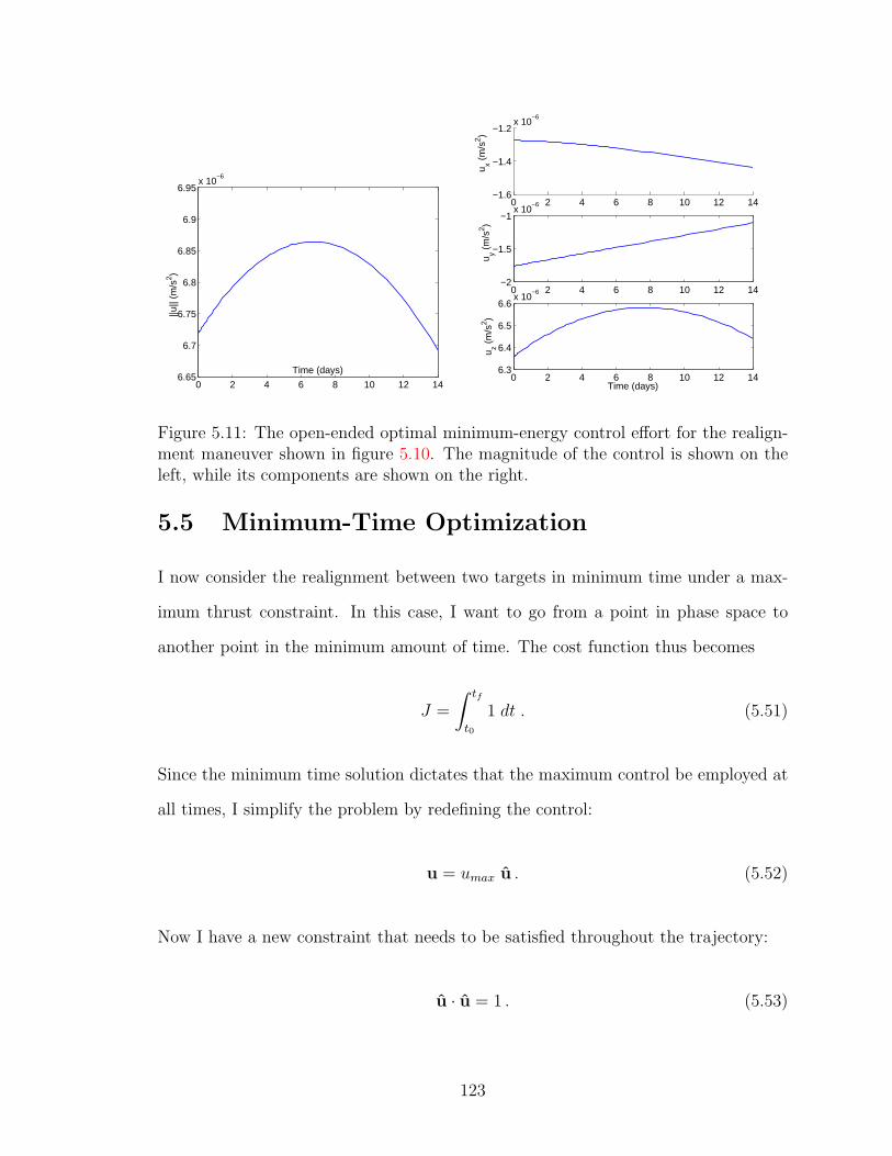
0 2 4 6 8 10 12 146.65
6.7
6.75
6.8
6.85
6.9
6.95x 10
−6
Time (days)
||u||
(m/s
2 )
0 2 4 6 8 10 12 14−1.6
−1.4
−1.2x 10
−6
u x (m
/s2 )
0 2 4 6 8 10 12 14−2
−1.5
−1x 10
−6
u y (m
/s2 )
0 2 4 6 8 10 12 146.3
6.4
6.5
6.6x 10
−6
Time (days)
u z (m
/s2 )
Figure 5.11: The open-ended optimal minimum-energy control effort for the realign-ment maneuver shown in figure 5.10. The magnitude of the control is shown on theleft, while its components are shown on the right.
5.5 Minimum-Time Optimization
I now consider the realignment between two targets in minimum time under a max-
imum thrust constraint. In this case, I want to go from a point in phase space to
another point in the minimum amount of time. The cost function thus becomes
J =
∫ tf
t0
1 dt . (5.51)
Since the minimum time solution dictates that the maximum control be employed at
all times, I simplify the problem by redefining the control:
u = umax u . (5.52)
Now I have a new constraint that needs to be satisfied throughout the trajectory:
u · u = 1 . (5.53)
123
I include this constraint in the Hamiltonian by augmenting it with additional La-
grange multipliers µ:
H = 1 + λT f(x) + umaxpu + µ(u · u− 1) . (5.54)
While the augmentation does not affect the adjoint differential equation, the optimal-
ity condition becomes
0 =∂H
∂u= umaxp + µu . (5.55)
Thus, the optimal control u can be obtained by solving this equation along with the
constraint equation 5.53,
u =
−umax
p|p| if |p| 6= 0
undetermined if p = 0 .
(5.56)
Previously, I used the optimality condition and Pontryagin’s Minimum Principle to
determine u∗(t) for all time t ∈ [t0, tf ] in terms of the extremal states, x∗, and adjoint
states, λ∗. If, however, there is a time interval [t1, t2] of finite duration during which
this principle provides no information about the optimal control, then the problem is
called singular and the interval [t1, t2] is called the singular interval.
In order to determine whether it is possible to have singular intervals, the case
where p is zero for finite time interval is considered. This condition implies that
derivatives of all orders of p should be zero during that time interval. In other words,
dkp
dtk= 0 k=1, 2, . . . (5.57)
124
Writing the differential equation for p from the adjoint states ODE,
p =
−λ1 + 2p2
−λ2 − 2p1
−λ3
, (5.58)
we can see that the singularity condition leads to λ = 0. However, for the open-end-
time problem under study there is another boundary condition. The Hamiltonian for
the open-end-time problems, where it is not an explicit function of time, is equal to
zero at all times (see Stengel [62] and Bryson & Ho [63] for details). Therefore, for
the CRTBP where H is not an explicit function of time:
H = 0 . (5.59)
For the singular intervals, we know that λ = 0. Substituting this equality in the
Hamiltonian, I obtain H = 1, which leads to a contradiction. Thus, there cannot be
singular intervals for this minimum-time optimization problem.
Substituting for u in the Euler-Lagrange equations, I obtain a 12-degree ODE in
terms of the state and adjoint state only:
x = f(t,x, λ)
λ = −(∂f(x, λ)
∂x
)T
λ , (5.60)
with boundary conditions
H = 0
x(t0)− x0
x(tf )− xf
= 0 . (5.61)
125

To apply numerical methods to solve this problem, the time boundaries for the BVP
must be defined explicitly. However, in this case, the time interval is [0, tf ], where
the end time for the BVP, tf , is an unknown parameter. In order to overcome
this problem, I redefine the system on the fixed-time interval [0, 1] by rewriting
the equation in terms of a new time variable:
τ =t
tf. (5.62)
Introducing tf as a new state variable, the extended differential equation becomes
dx
dτ= tf f(t,x,u)
dλ
dτ= −tf
(∂f(x, λ)
∂x
)T
λ
dtfdτ
= 0 . (5.63)
Now the 13-dimensional BVP can be solved.
I first employed the collocation algorithm to solve the time-optimal transfer from
Earth to L2. I solved the problem with a range of maximum-allowable control as
shown in figure 5.12. The minimum time-of-flight as a function of maximum control
is shown in figure 5.13. Position and control histories for a sample trajectory are
shown in figure 5.14.
Next, I looked at the LOS realignment problem. The requirement for the re-
alignment is that, at the final time, the occulter must be positioned to look at a
pre-specified star with the inertial positional direction, e. Recall that, at different
times, the position and velocity of the occulter are given as below:
rocc = rtel +R e (5.64)
vocc = vtel + ω ×R e (5.65)
126
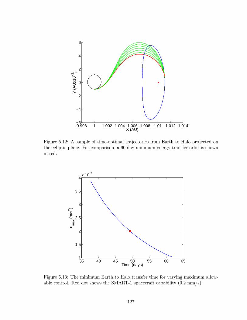
0.998 1 1.002 1.004 1.006 1.008 1.01 1.012 1.014−6
−4
−2
0
2
4
6
X (AU)
Y (
AU
x10−
3 )
Figure 5.12: A sample of time-optimal trajectories from Earth to Halo projected onthe ecliptic plane. For comparison, a 90 day minimum-energy transfer orbit is shownin red.
35 40 45 50 55 60 651
1.5
2
2.5
3
3.5
4x 10
−4
Time (days)
u max
(m
/s2 )
Figure 5.13: The minimum Earth to Halo transfer time for varying maximum allow-able control. Red dot shows the SMART-1 spacecraft capability (0.2 mm/s).
127
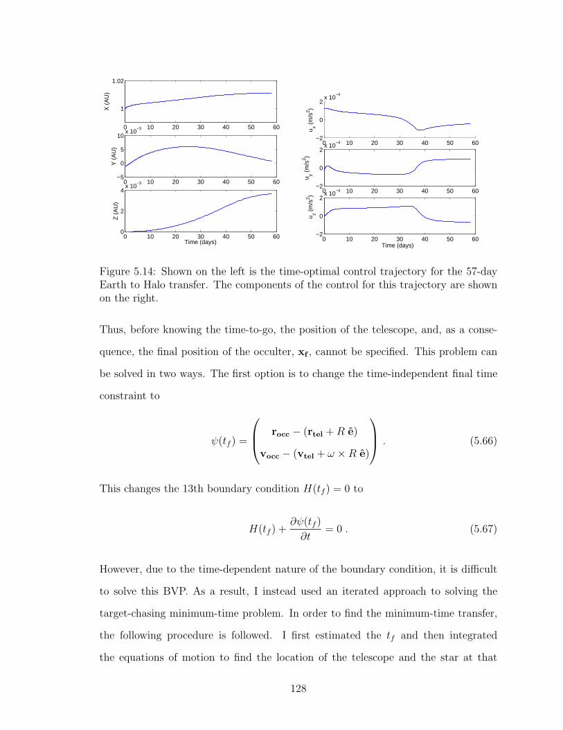
0 10 20 30 40 50 60
1
1.02
X (
AU
)
0 10 20 30 40 50 60−5
0
5
10x 10
−3
Y (
AU
)
0 10 20 30 40 50 600
2
4x 10
−3
Time (days)
Z (
AU
)
0 10 20 30 40 50 60−2
0
2x 10
−4
u x (m
/s2 )
0 10 20 30 40 50 60−2
0
2x 10
−4
u y (m
/s2 )
0 10 20 30 40 50 60−2
0
2x 10
−4
Time (days)
u z (m
/s2 )
Figure 5.14: Shown on the left is the time-optimal control trajectory for the 57-dayEarth to Halo transfer. The components of the control for this trajectory are shownon the right.
Thus, before knowing the time-to-go, the position of the telescope, and, as a conse-
quence, the final position of the occulter, xf , cannot be specified. This problem can
be solved in two ways. The first option is to change the time-independent final time
constraint to
ψ(tf ) =
rocc − (rtel +R e)
vocc − (vtel + ω ×R e)
. (5.66)
This changes the 13th boundary condition H(tf ) = 0 to
H(tf ) +∂ψ(tf )
∂t= 0 . (5.67)
However, due to the time-dependent nature of the boundary condition, it is difficult
to solve this BVP. As a result, I instead used an iterated approach to solving the
target-chasing minimum-time problem. In order to find the minimum-time transfer,
the following procedure is followed. I first estimated the tf and then integrated
the equations of motion to find the location of the telescope and the star at that
128
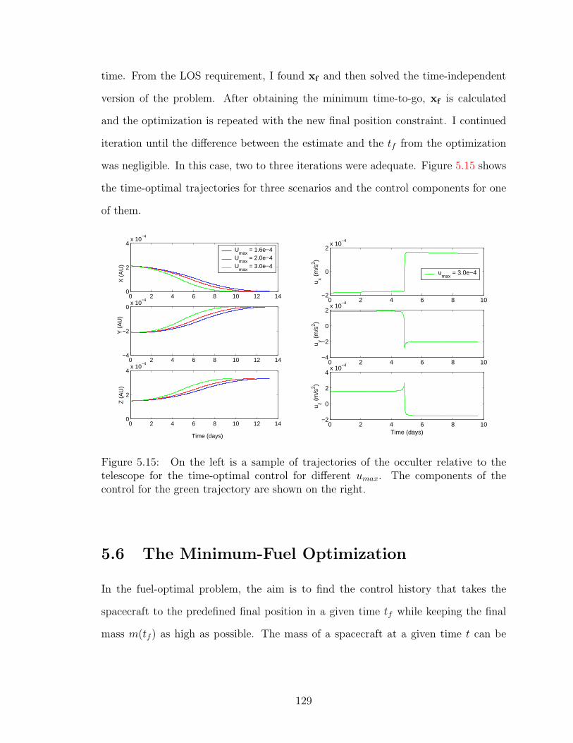
time. From the LOS requirement, I found xf and then solved the time-independent
version of the problem. After obtaining the minimum time-to-go, xf is calculated
and the optimization is repeated with the new final position constraint. I continued
iteration until the difference between the estimate and the tf from the optimization
was negligible. In this case, two to three iterations were adequate. Figure 5.15 shows
the time-optimal trajectories for three scenarios and the control components for one
of them.
0 2 4 6 8 10 12 140
2
4x 10
−4
X (
AU
)
0 2 4 6 8 10 12 14−4
−2
0x 10
−4
Y (
AU
)
0 2 4 6 8 10 12 140
2
4x 10
−4
Time (days)
Z (
AU
)
Umax
= 1.6e−4U
max = 2.0e−4
Umax
= 3.0e−4
0 2 4 6 8 10−2
0
2x 10
−4
u x (m
/s2 )
0 2 4 6 8 10−4
−2
0
2x 10
−4
u y (m
/s2 )
0 2 4 6 8 10−2
0
2
4x 10
−4
Time (days)
u z (m
/s2 )
umax
= 3.0e−4
Figure 5.15: On the left is a sample of trajectories of the occulter relative to thetelescope for the time-optimal control for different umax. The components of thecontrol for the green trajectory are shown on the right.
5.6 The Minimum-Fuel Optimization
In the fuel-optimal problem, the aim is to find the control history that takes the
spacecraft to the predefined final position in a given time tf while keeping the final
mass m(tf ) as high as possible. The mass of a spacecraft at a given time t can be
129

determined by the relationship
m(t) = m0 − mt , (5.68)
where m is the constant propellant flow rate and m0 is the mass of the spacecraft at
the initial time. Assuming that the total change in the mass throughout the trajectory
is negligible, Newton’s second law of motion can be written as
|u|m0 ≈ m Vex/b , (5.69)
and it follows that
m(tf ) ≈ m0 −tf |u|Vex/b
, (5.70)
where Vex/b is the velocity of exhaust with respect to the body and u is the iner-
tial acceleration due to spacecraft propulsion, the control input that has been used
throughout this chapter. The velocity of the exhaust depends on the specifications
of the spacecraft thruster.
The constant mass approximation is a very good one for the LOS realignment
maneuver since such maneuvers take at most a few weeks. For the Earth-Halo transfer
case, this assumption is not a very good one, but the more complicated optimization,
where the dynamics of the change in mass is included in the dynamical equations, is
not considered, since the Earth-Halo transfer is not the main objective of this study.
With this approximation, maximizing final mass is equivalent to minimizing the
magnitude of the control throughout the trajectory. For this case, the cost function
is
J =
∫ tf
t0
|u| dt . (5.71)
130
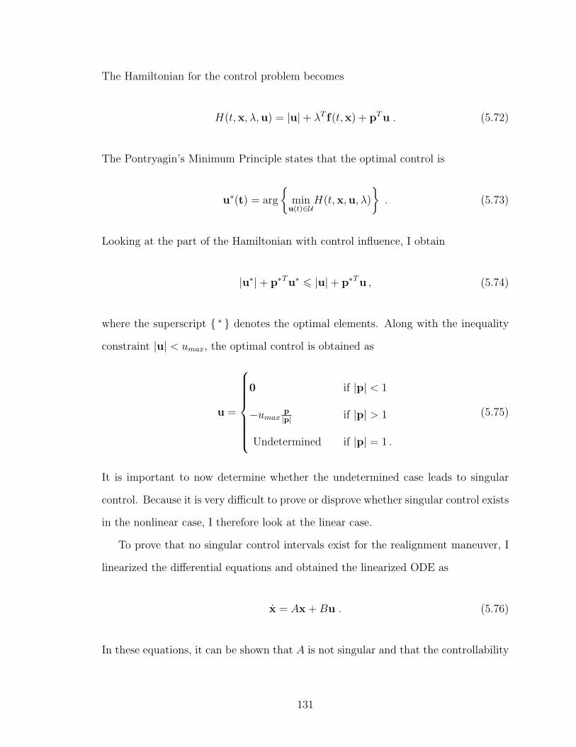
The Hamiltonian for the control problem becomes
H(t,x, λ,u) = |u|+ λT f(t,x) + pTu . (5.72)
The Pontryagin’s Minimum Principle states that the optimal control is
u∗(t) = arg
min
u(t)∈UH(t,x,u, λ)
. (5.73)
Looking at the part of the Hamiltonian with control influence, I obtain
|u∗|+ p∗Tu∗ 6 |u|+ p∗Tu , (5.74)
where the superscript ∗ denotes the optimal elements. Along with the inequality
constraint |u| < umax, the optimal control is obtained as
u =
0 if |p| < 1
−umaxp|p| if |p| > 1
Undetermined if |p| = 1 .
(5.75)
It is important to now determine whether the undetermined case leads to singular
control. Because it is very difficult to prove or disprove whether singular control exists
in the nonlinear case, I therefore look at the linear case.
To prove that no singular control intervals exist for the realignment maneuver, I
linearized the differential equations and obtained the linearized ODE as
x = Ax +Bu . (5.76)
In these equations, it can be shown that A is not singular and that the controllability
131
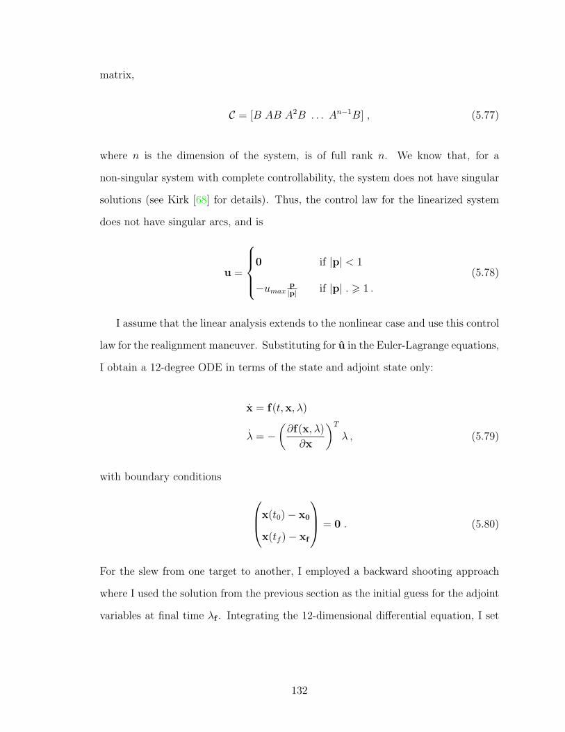
matrix,
C = [B AB A2B . . . An−1B] , (5.77)
where n is the dimension of the system, is of full rank n. We know that, for a
non-singular system with complete controllability, the system does not have singular
solutions (see Kirk [68] for details). Thus, the control law for the linearized system
does not have singular arcs, and is
u =
0 if |p| < 1
−umaxp|p| if |p| . > 1 .
(5.78)
I assume that the linear analysis extends to the nonlinear case and use this control
law for the realignment maneuver. Substituting for u in the Euler-Lagrange equations,
I obtain a 12-degree ODE in terms of the state and adjoint state only:
x = f(t,x, λ)
λ = −(∂f(x, λ)
∂x
)T
λ , (5.79)
with boundary conditions
x(t0)− x0
x(tf )− xf
= 0 . (5.80)
For the slew from one target to another, I employed a backward shooting approach
where I used the solution from the previous section as the initial guess for the adjoint
variables at final time λf . Integrating the 12-dimensional differential equation, I set
132
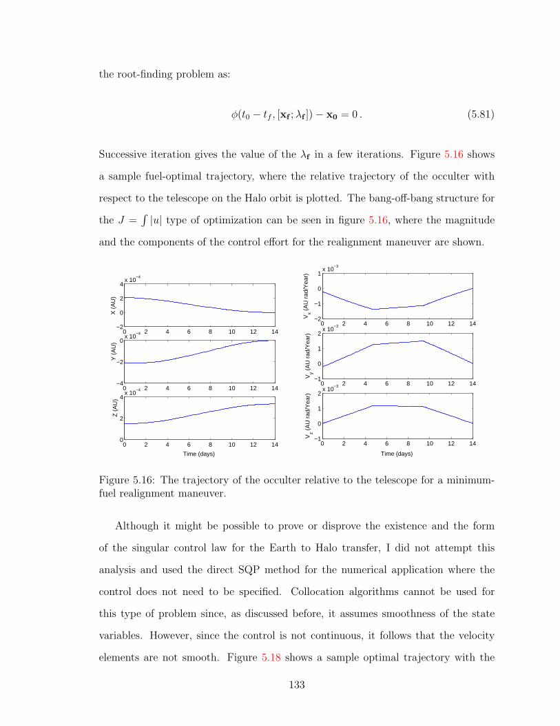
the root-finding problem as:
φ(t0 − tf , [xf ;λf ])− x0 = 0 . (5.81)
Successive iteration gives the value of the λf in a few iterations. Figure 5.16 shows
a sample fuel-optimal trajectory, where the relative trajectory of the occulter with
respect to the telescope on the Halo orbit is plotted. The bang-off-bang structure for
the J =∫|u| type of optimization can be seen in figure 5.16, where the magnitude
and the components of the control effort for the realignment maneuver are shown.
0 2 4 6 8 10 12 14−2
0
2
4x 10
−4
X (
AU
)
0 2 4 6 8 10 12 14−4
−2
0x 10
−4
Y (
AU
)
0 2 4 6 8 10 12 140
2
4x 10
−4
Time (days)
Z (
AU
)
0 2 4 6 8 10 12 14−2
−1
0
1x 10
−3
Vx (
AU
rad
/Yea
r)
0 2 4 6 8 10 12 14−1
0
1
2x 10
−3
Vy (
AU
rad
/Yea
r)
0 2 4 6 8 10 12 14−1
0
1
2x 10
−3
Time (days)
Vz (
AU
rad
/Yea
r)
Figure 5.16: The trajectory of the occulter relative to the telescope for a minimum-fuel realignment maneuver.
Although it might be possible to prove or disprove the existence and the form
of the singular control law for the Earth to Halo transfer, I did not attempt this
analysis and used the direct SQP method for the numerical application where the
control does not need to be specified. Collocation algorithms cannot be used for
this type of problem since, as discussed before, it assumes smoothness of the state
variables. However, since the control is not continuous, it follows that the velocity
elements are not smooth. Figure 5.18 shows a sample optimal trajectory with the
133

0 2 4 6 8 10 12 140
0.2
0.4
0.6
0.8
1
1.2
1.4
1.6
1.8x 10
−4
Time (days)
||u||
(m/s
2 )
0 2 4 6 8 10 12 14
0
2x 10
−4
u x (m
/s2 )
0 2 4 6 8 10 12 14−2
0
2x 10
−4
u y (m
/s2 )
0 2 4 6 8 10 12 14
0
2x 10
−4
Time (days)
u z (m
/s2 )
Figure 5.17: The minimum-fuel control effort for the realignment maneuver shown infigure 5.16. The magnitude of the control is shown on the left, while its componentsare shown on the right.
same boundary conditions that were defined in the previous sections. Figure 5.19
show the optimal control effort used for this trajectory.
5.7 Impulsive Thrust: Minimum-Fuel Optimiza-
tion
Finally, I looked at the fuel-optimal impulsive control problem. The trajectories
that take the occulter from one target star LOS to another with minimum fuel were
studied for an impulsive thrusting system. As seen in figure 5.19, for the continuous
case, the fuel-optimal solution is a bang-off-bang control. As the upper bound on |u|
is increased, the bang-off-bang nature of the control is retained, with the thrusting
phase (bang part) becoming increasingly small. In the limit, we obtain the impulsive
optimal control solution where the velocity instantaneously changes at the beginning
and at the end of the interval. This corresponds to an impulsive maneuver like the
one that would be obtained from an impulsive chemical rocket. In this case, the
134
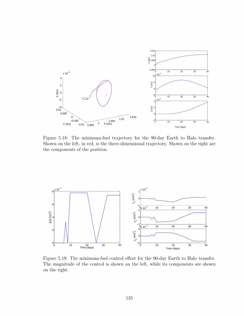
0.9951
1.0051.01
1.015
−0.01−0.0050
0.0050.01
−4
−2
0
2
4
x 10−3
X (AU)Y (AU)
Z (
AU
)
0 10 20 30 400.995
1
1.005
1.01
1.015
X (
AU
)
0 10 20 30 40−5
0
5
10x 10
−3
Y (
AU
)
0 10 20 30 40−2
0
2
4x 10
−3
Time (days)
Z (
AU
)
Figure 5.18: The minimum-fuel trajectory for the 90-day Earth to Halo transfer.Shown on the left, in red, is the three-dimensional trajectory. Shown on the right arethe components of the position.
0 10 20 30 400
2
4
6
8x 10
−4
Time (days)
||u||
(m/s
2 )
0 10 20 30 40−1
0
1x 10
−3
u x (m
/s2 )
0 10 20 30 40−1
0
1x 10
−3
u y (m
/s2 )
0 10 20 30 40−5
0
5x 10
−4
Time (days)
u z (m
/s2 )
Figure 5.19: The minimum-fuel control effort for the 90-day Earth to Halo transfer.The magnitude of the control is shown on the left, while its components are shownon the right.
135
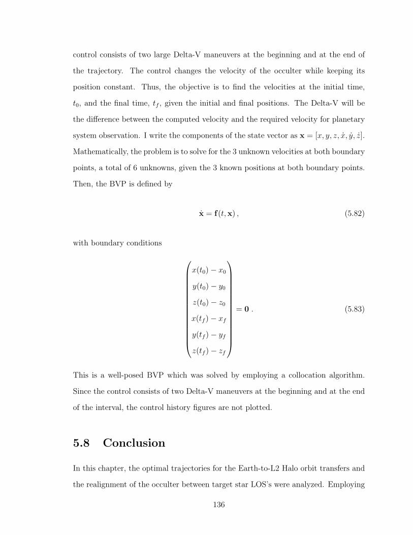
control consists of two large Delta-V maneuvers at the beginning and at the end of
the trajectory. The control changes the velocity of the occulter while keeping its
position constant. Thus, the objective is to find the velocities at the initial time,
t0, and the final time, tf , given the initial and final positions. The Delta-V will be
the difference between the computed velocity and the required velocity for planetary
system observation. I write the components of the state vector as x = [x, y, z, x, y, z].
Mathematically, the problem is to solve for the 3 unknown velocities at both boundary
points, a total of 6 unknowns, given the 3 known positions at both boundary points.
Then, the BVP is defined by
x = f(t,x) , (5.82)
with boundary conditions
x(t0)− x0
y(t0)− y0
z(t0)− z0
x(tf )− xf
y(tf )− yf
z(tf )− zf
= 0 . (5.83)
This is a well-posed BVP which was solved by employing a collocation algorithm.
Since the control consists of two Delta-V maneuvers at the beginning and at the end
of the interval, the control history figures are not plotted.
5.8 Conclusion
In this chapter, the optimal trajectories for the Earth-to-L2 Halo orbit transfers and
the realignment of the occulter between target star LOS’s were analyzed. Employing
136

Euler-Lagrange, SQP, and shooting algorithms, I obtained the energy, time, and fuel
optimal control for continuous thrusters and the fuel-optimal control for impulsive
thrusters. The trajectories for various boundary conditions were solved. These tra-
jectories are used in the next chapter for the global optimization of the space telescopy
mission consisting of a telescope and a constellation of occulters.
137
Chapter 6
Global Optimization of the
Mission: The Traveling Salesman
Problem
138

In the previous chapter, the trajectory optimization for star target-to-target ma-
neuvers was conducted, where I found the minimum Delta-V that is needed for the
realignment processes. Here, the sequencing and timing of the imaging session is
examined in order to globally optimize the full occulter-based telescopy mission.
This chapter aims to arrive at the algorithms that optimize the different mission
scenarios from beginning to end, and that reduce the complexities of the various
missions to simple graphs, where a side-by-side comparison of the advantages and
disadvantages of these missions is possible. This makes possible a trade-off study,
using different control strategies, in terms of cost, i.e., the total Delta-V for the
mission, and scientific achievement, i.e., the number of planetary systems that are
imaged.
In the first section, the results from the previous chapter are combined, and the
cost of realignment as a function of mission parameters is obtained.
In the second section, a more detailed overview of the realistic mission conditions
and constraints is given. It is explained how the global optimization problem can
be reduced to a sorting problem that is similar to the Traveling Salesman Problem
(TSP).
In the third section, the well-known Traveling Salesman Problem (TSP) is intro-
duced. The mathematical formulation and numerical solution methods are shown,
and the global optimization problem is solved based on a TSP approximation.
In the fourth section, a mathematical model for the realistic mission optimization
is produced, which is akin to a Time-Dependent TSP (TDTSP).
In the fifth section, numerical methods to solve the TDTSP are discussed. These
numerical methods are applied to various mission concepts with no control limitations.
In the sixth section, a feasibility study of the mission is performed by analyzing
possible scenarios with the capabilities of the SMART-1 spacecraft.
139
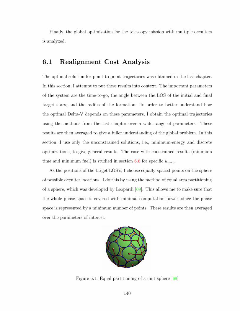
Finally, the global optimization for the telescopy mission with multiple occulters
is analyzed.
6.1 Realignment Cost Analysis
The optimal solution for point-to-point trajectories was obtained in the last chapter.
In this section, I attempt to put these results into context. The important parameters
of the system are the time-to-go, the angle between the LOS of the initial and final
target stars, and the radius of the formation. In order to better understand how
the optimal Delta-V depends on these parameters, I obtain the optimal trajectories
using the methods from the last chapter over a wide range of parameters. These
results are then averaged to give a fuller understanding of the global problem. In this
section, I use only the unconstrained solutions, i.e., minimum-energy and discrete
optimizations, to give general results. The case with constrained results (minimum
time and minimum fuel) is studied in section 6.6 for specific umax.
As the positions of the target LOS’s, I choose equally-spaced points on the sphere
of possible occulter locations. I do this by using the method of equal area partitioning
of a sphere, which was developed by Leopardi [69]. This allows me to make sure that
the whole phase space is covered with minimal computation power, since the phase
space is represented by a minimum number of points. These results are then averaged
over the parameters of interest.
Figure 6.1: Equal partitioning of a unit sphere [69]
140

Using the optimization method developed above, I find the Delta-V that is needed
to go between these targets at 20 equally placed locations in the Halo orbit. In figure
6.2, the Delta-V resulting from these millions of optimizations are averaged for the
minimum-energy optimization, giving Delta-V as an approximate function of the
radius and the LOS angle for a transfer time of 2 weeks.
Figure 6.2: The surface of Delta-Vs as a function of distance from the telescope, andthe angle between the LOS vectors of consecutively imaged stars for minimum-energyoptimization (∆t = 2 weeks).
In order to make the mission analysis more realistic, the top 100 TPF-C target
stars given in [59] were used. I found the Delta-V for the realignment between each
target for impulsive maneuvers, as shown in figure 6.3. In the figure, the identification
numbers of the stars are sorted in ascending declination.
6.2 Defining the Global Optimization Problem
Now that the relevant optimal trajectories between any two given star-imaging ses-
sions have been found, it is important to examine the sequencing and timing of the
imaging sessions, in order to minimize the global cost of the mission. This section
gives an overview of the constraints that are associated with an occulter-based tele-
scopy mission. I explain how the global optimization problem can be reduced to a
141
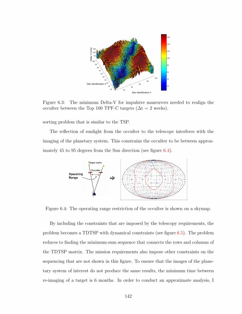
20
40
60
80
100
10
20
30
40
50
60
70
80
90
100
50
100
150
Star Identification #
Star Identification #
Del
ta−
V (
m/s
)
20
40
60
80
100
120
140
160
Figure 6.3: The minimum Delta-V for impulsive maneuvers needed to realign theocculter between the Top 100 TPF-C targets (∆t = 2 weeks).
sorting problem that is similar to the TSP.
The reflection of sunlight from the occulter to the telescope interferes with the
imaging of the planetary system. This constrains the occulter to be between approx-
imately 45 to 95 degrees from the Sun direction (see figure 6.4).
Figure 6.4: The operating range restriction of the occulter is shown on a skymap.
By including the constraints that are imposed by the telescopy requirements, the
problem becomes a TDTSP with dynamical constraints (see figure 6.5). The problem
reduces to finding the minimum-sum sequence that connects the rows and columns of
the TDTSP matrix. The mission requirements also impose other constraints on the
sequencing that are not shown in this figure. To ensure that the images of the plane-
tary system of interest do not produce the same results, the minimum time between
re-imaging of a target is 6 months. In order to conduct an approximate analysis, I
142
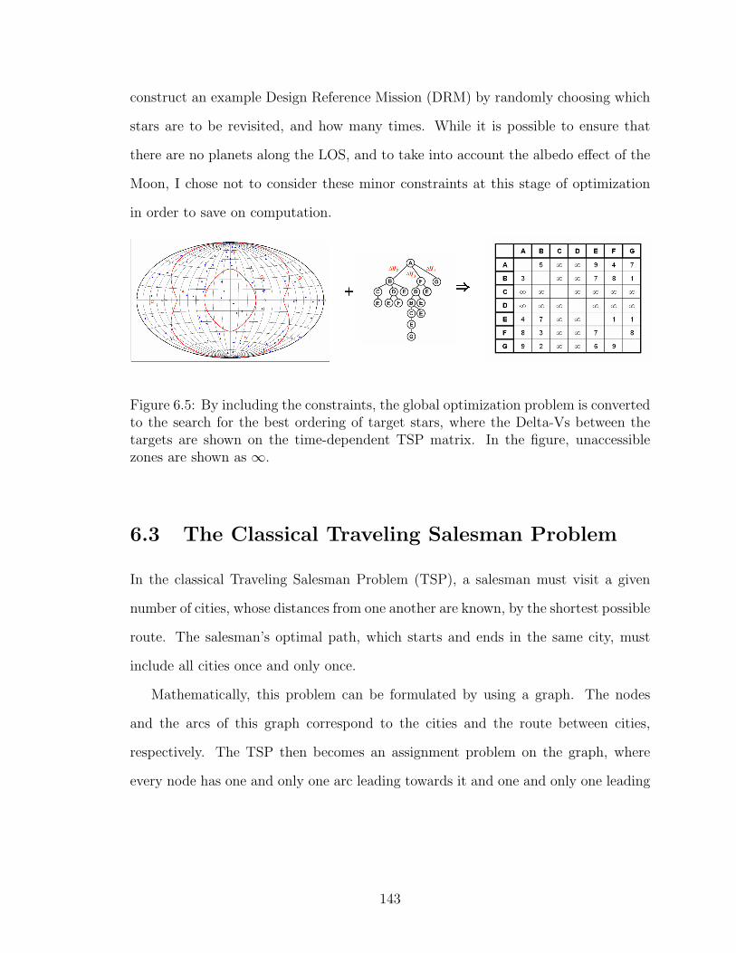
construct an example Design Reference Mission (DRM) by randomly choosing which
stars are to be revisited, and how many times. While it is possible to ensure that
there are no planets along the LOS, and to take into account the albedo effect of the
Moon, I chose not to consider these minor constraints at this stage of optimization
in order to save on computation.
Figure 6.5: By including the constraints, the global optimization problem is convertedto the search for the best ordering of target stars, where the Delta-Vs between thetargets are shown on the time-dependent TSP matrix. In the figure, unaccessiblezones are shown as ∞.
6.3 The Classical Traveling Salesman Problem
In the classical Traveling Salesman Problem (TSP), a salesman must visit a given
number of cities, whose distances from one another are known, by the shortest possible
route. The salesman’s optimal path, which starts and ends in the same city, must
include all cities once and only once.
Mathematically, this problem can be formulated by using a graph. The nodes
and the arcs of this graph correspond to the cities and the route between cities,
respectively. The TSP then becomes an assignment problem on the graph, where
every node has one and only one arc leading towards it and one and only one leading
143
away from it. This can be expressed by employing the variable
xij =
1 if arc(i,j) is in the tour,
0 otherwise,
(6.1)
for i = 1, 2, . . . , n and j = 1, 2, . . . , n, and where n is the number of cities, or in
our case, stars to visit.
On this graph, the TSP becomes the arc length minimization problem given below:
Min∑i,j
cij xij
s. t.∑
i
xij = 1 ∀ j 6= i
∑j
xij = 1 ∀ i 6= j
xij ∈ 0, 1 ∀ i, j . (6.2)
Here, cij are the elements of the cost matrix, c. Every element of this matrix represents
the distance between two cities.
However, this formulation may not give the desired, single loop that connects all
the nodes. Multiple, unconnected loops, or “subtours”, may result. To overcome
this problem, additional constraints must be added to the formulation. The Miller-
Tucker-Zemlin formulation [70], which introduces new variables, ui for i = 1, . . . , n
for subtour exclusion, is one of the most well-known formulations:
u1 = 1
2 6 ui 6 n ∀ i 6= 1
ui − uj + 1 6 (n− 1)(1− xij) ∀ i 6= 1, ∀ j 6= 1 . (6.3)
144
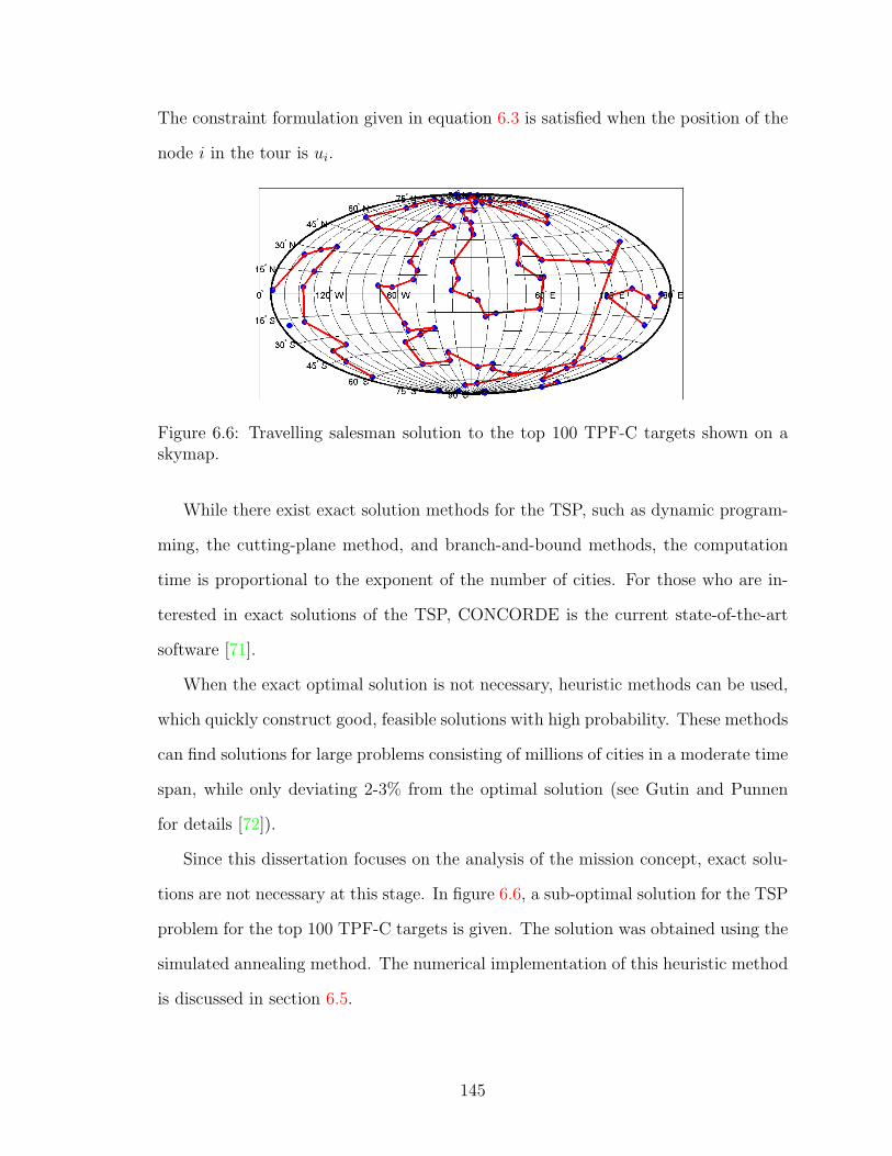
The constraint formulation given in equation 6.3 is satisfied when the position of the
node i in the tour is ui.
Figure 6.6: Travelling salesman solution to the top 100 TPF-C targets shown on askymap.
While there exist exact solution methods for the TSP, such as dynamic program-
ming, the cutting-plane method, and branch-and-bound methods, the computation
time is proportional to the exponent of the number of cities. For those who are in-
terested in exact solutions of the TSP, CONCORDE is the current state-of-the-art
software [71].
When the exact optimal solution is not necessary, heuristic methods can be used,
which quickly construct good, feasible solutions with high probability. These methods
can find solutions for large problems consisting of millions of cities in a moderate time
span, while only deviating 2-3% from the optimal solution (see Gutin and Punnen
for details [72]).
Since this dissertation focuses on the analysis of the mission concept, exact solu-
tions are not necessary at this stage. In figure 6.6, a sub-optimal solution for the TSP
problem for the top 100 TPF-C targets is given. The solution was obtained using the
simulated annealing method. The numerical implementation of this heuristic method
is discussed in section 6.5.
145
6.4 Mathematical Formulation of the Global Op-
timization Problem
In this section, the mathematical formulation for the realignment problem is obtained,
starting from the classical TSP formulation. There are four major differences between
the classical TSP and the realignment problem. First, the cost matrix in our case is
time dependent due to the motion of the telescope on the Halo orbit, the change in
the star directions relative to the telescope, and the evolution of the exclusion zone.
Second, additional constraints must be satisfied. Third, the occulter may visit some
of the star targets more than once. And finally, the occulter does not have to visit
all the possible star targets.
I formulate the travelling occulter problem given the following parameters: the
total number of observations, Ntot, the identification number of the stars that can be
imaged more than once, ir, and the slew time between imaging sessions, ∆t. For the
sake of simplicity, I assumed that the maximum number of visits to any given star
was two. The results can easily be extended to the case with more than two visits.
The formulation of the problem is set such that the multiple occulter case is obtained
with minimal modification of this formulation, as seen in section 6.7.
6.4.1 Cost function
First, let us define the cost function for the problem with only a single measurement
for each star. The time interval between each observation, ∆t, is assumed to be
constant in order to simplify the problem. Then, ti, the time when the ith target is
being imaged, becomes ∆t ui, which is only a function of how many observations were
conducted before the current target. Thus, the cost matrix that is to be minimized
146
can be expressed as:
Min∑i,j
c(i, j, ui) xij . (6.4)
In this formulation, c(i, j, ui) is a three-dimensional matrix at each time instance
given with ui, which can be precomputed.
At each time interval, the constraints, such as the stars which are non-imageable
due to their location relative to the Sun, are calculated. For the stars that cannot be
observed at that time, the c(i, j, ui) is set to infinity.
The sequence after the maximum visit number should not matter in the total cost
computation. In order to ensure that it is excluded, the matrix elements of c(i, j, ui)
for all ui greater than the user-specified maximum number of total observations, Ntot,
are set to zero.
c(i, j, ui) = 0 for ui > Ntot + 1 (6.5)
Thus, the algorithm only minimizes cost for the Delta-V budget up to this value and
does not take into account the remaining nodes.
6.4.2 Including the revisits into the formulation
In this section, a method to include the option of revisiting sample stars with identi-
fication numbers ir is introduced into the formulation. As stated, I assume that the
maximum number of imaging of a given star is two. Higher numbers can easily be
introduced into the formulation without loss of generality.
First, I double the number of nodes such that each star now corresponds to two
nodes, one for the first visit and the other for the second visit. i and j are redefined to
be double the size to i = 1, 2, . . . , 2n and j = 1, 2, . . . , 2n, where n is the number
147
stars. In this notation, elements of i and j from 1 through n represent a first visit of
a target star with the identification number i or j. The elements from n+ 1 through
2n represent a second visit of a target star with the identification number i − n or
j − n. Correspondingly, I redefine the cost matrix to be double the size:
c(i, j, ui) :=
c(i, j, ui) c(i, j, ui)
c(i, j, ui) c(i, j, ui)
. (6.6)
If a star with identification number k is not allowed to be revisited, the cost for a
second visit is set to infinity (or a very large number):
c(k + n, :, :) = ∞ , c(:, k + n, :) = ∞ . (6.7)
This formulation enables me to keep the TSP formulation for the xij:
∑i
xij = 1 ∀ j 6= i
∑j
xij = 1 ∀ i 6= j
xij ∈ 0, 1 ∀ i, j . (6.8)
The revisits, if they happen, should be after a certain amount of time. For a given
star with identification number i and position in the sequence ui, its revisit partner
with position ui+n should be separated by a minimum distance
ui +Nrevisit 6 ui+n , (6.9)
where n is the number of stars of interest and Nrevisit is the minimum re-imaging
interval. These constraints ensure that the revisit only happens after a certain amount
of time has passed. Since the time between each observation is assumed to be constant,
148
ti = ∆t ui is only a function of how many observations were conducted before. For
example, for a realignment maneuver of two weeks, and a minimum allowable revisit
time of six months, Nrevisit = 12.
6.4.3 Full Formulation
The full formulation for the mathematical model can thus be written as:
Min∑i,j
c(i, j, ui) xij
s. t.∑
i
xij = 1 ∀ j 6= i
∑j
xij = 1 ∀ i 6= j
u1 = 1
2 6 ui 6 2n ∀ i 6= 1
ui − uj + 1 6 (2n− 1)(1− xij) ∀ i 6= 1, ∀ j 6= 1
ui +Nrevisit 6 ui+n ∀ i
xij ∈ 0, 1 ∀ i, j , (6.10)
where c is a precalculated three-dimensional matrix. For the minimum-fuel problem,
the elements of c are the Delta-V calculated in the previous sections. Without loss of
generality, u1 is set to one, which can be changed for different starting stars.
For the minimum-time optimization problem, the elements of the c matrix are the
time-to-go between each target. In this case, the time spent between each realignment
is no longer a constant. The cost and the constraints that are associated with the arc
i− j are now dependent on time ti at position ui.
The time at a given arc can be expressed as the sum of all the costs, or the
149
time-to-go, before that node:
t1 = 0
tk =∑i,j
c(i, j, ti) xij ∀ i s.t. ui = 1, . . . , k − 1 and ∀ j s.t. uj = 2, . . . , k (6.11)
Here, the indices of the stars which have already been visited must first be identified
from the elements of u. Then, the total time is calculated by summing all the pre-
vious time intervals. The cost function c is a continuous function of time, since the
observable stars change with time while the time is dependent upon all the previous
observations. This formulation is a much more complicated nonlinear programming
problem.
6.5 Numerical Methods Employed for Solving the
Global Optimization Problem
As discussed before, I do not implement the exact solution methods for the optimiza-
tion problem. In line with the scope of this dissertation, which is the analysis of the
mission concept, I use heuristic methods, which deviate only a few percent from the
optimal solution, and quickly construct good, feasible solutions with high probability.
While solving the classical TSP, I implemented the tabu search [73], ant colony
optimization [74], cross-entropy [75], and simulated annealing methods [76] to famil-
iarize myself with the heuristic methods. They all performed well.
The ant colony optimization and cross-entropy methods employ a swarm of can-
didate solutions. These methods are not suitable for our problem, because of the
existence of a high level of constraints. As far as the cross-entropy method is con-
cerned, one infeasible solution in a group would bring the statistical average of the
group up, but trying to impose the constraints on the elements is against the spirit
150
of the swarms of trials and averaging. As for the ant colony optimization, it is not
apparent how the constraint can be imposed that prevents the same star from being
revisited before a certain amount of time.
I chose to use simulated annealing rather than a tabu search, since, due to the
constraints, the optimal solution and initial feed might be in separated parts of the
search space, and random motion given in simulated annealing might be of use to get
out of local minima.
Next, I explain the implementation of simulated annealing for the problem at
hand.
6.5.1 Simulated annealing
Developed by Kirkpatrick et al. [76], simulated annealing is a global optimization
method suitable for problems with a large search space. The method is inspired by
the way crystalline structures are formed in the thermal annealing process, such as
the production of high-strength steel.
The analogy between the physical annealing process and the numerical optimiza-
tion is such that the temperature change is akin to the time spent in the optimization,
and the energy level is analogous to the cost function to be minimized. Similarly to
the physics of atoms under the annealing process, simulated annealing generates ran-
dom solutions in the neighborhood of the old one. Initially, when the temperature is
high (the initial stages of optimization), random moves which lead to higher energy
(higher cost) levels are allowed frequently, but as the system cools down (optimization
time increases), the tendency to allow moves which increase the energy is reduced.
The algorithm becomes more like a downhill search method.
151

Algorithm Pseudo-Code
Below is the pseudo-code for the simulated annealing algorithm used in the global
optimization problem.
input: X0, Tmin, kappa
energy = cost(X0);
X = X0;
while T > Tmin
X_new = neighbor(X);
energy_new = cost(X);
delta = energy - energy_new;
if (delta > 0) or (exp(delta/T) > random())
X = X_new;
energy = energy_new;
T = T*kappa;
end
output: X, energy
Here, X is a vector which contains the visiting sequence of each star (and visiting
partners, if they exist). Temperature is represented by T, the freezing temperature by
Tmin and the cooling constant by kappa. Three functions are used in the algorithm;
random() is a uniform-distribution random number generator in the interval (0, 1);
cost is the cost function for a given visiting sequence; and neighbor is a function which
generates random visiting strings in the neighborhood of X.
For the constants in the algorithm, a cooling constant of ∼0.99 and initial temper-
atures in the range of 10-40 degrees gave good results. I set the freezing temperature
to be one degree.
152
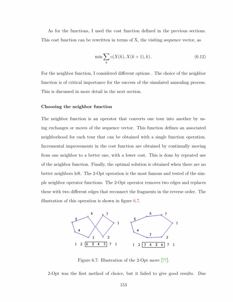
As for the functions, I used the cost function defined in the previous sections.
This cost function can be rewritten in terms of X, the visiting sequence vector, as
min∑
k
c(X(k), X(k + 1), k) . (6.12)
For the neighbor function, I considered different options . The choice of the neighbor
function is of critical importance for the success of the simulated annealing process.
This is discussed in more detail in the next section.
Choosing the neighbor function
The neighbor function is an operator that converts one tour into another by us-
ing exchanges or moves of the sequence vector. This function defines an associated
neighborhood for each tour that can be obtained with a single function operation.
Incremental improvements in the cost function are obtained by continually moving
from one neighbor to a better one, with a lower cost. This is done by repeated use
of the neighbor function. Finally, the optimal solution is obtained when there are no
better neighbors left. The 2-Opt operation is the most famous and tested of the sim-
ple neighbor operator functions. The 2-Opt operator removes two edges and replaces
these with two different edges that reconnect the fragments in the reverse order. The
illustration of this operation is shown in figure 6.7.
Figure 6.7: Illustration of the 2-Opt move [77].
2-Opt was the first method of choice, but it failed to give good results. Due
153

to the high number of constraints involved in our problem, a constraint was broken
almost every time when a part of the sequence was reversed. I decided not to use this
operator.
Consider that, as the simulated annealing proceeds, the energy of the state will be
lower than that of a random state. Thus, if the neighbor function results in arbitrary
states, these moves will all be rejected after a few steps. Therefore, in simulated
annealing, the neighbor function should be chosen such that the neighbors and the
current tour have similar energy levels. As a result, I opted for an operation where I
swapped the two consecutive stars, swap (X(k), X(k+1)), rather than arbitrary stars.
Additionally, if the operator does not obey the constraints by default, many fruit-
less trials result. I avoided this by choosing the initial guess to satisfy all the con-
straints, and by making sure that all the neighbor perpetration satisfy the constraint.
When swapping the stars in consecutive positions, I checked whether the swap oper-
ation leads to a minimum distance between the pair partners, a star and its revisit
partner, of less than Nrevisit. If so, the swap is not performed and another random k
is chosen to swap (X(k), X(k+1)). This ensures that, as long as the initial sequence
obeys the minimum separation between pairs of less than Nrevisit, the neighbor will
also obey this constraint. By not breaking any constraints, the algorithm is able to
move through the neighborhood quickly.
However, the neighbor function should be able to reach every possible state of
the system, and the swapping that is described above may not ensure this property,
because it is done in pairs. To overcome this problem, I used three more operators
that enlarge the neighborhood sufficiently to avoid getting stuck in local minima.
These are the following operators:
1. Swap random star pairs: Two random pairs, i, i+ n and j, j + n, two stars
and their revisit partners, are swapped, swap (X(ui,ui+n), X(uj,uj+n)).
2. Mutate random star pairs (1): Two random pairs, i, i + n and j, j + n,
154

are mutated such that the locations of i and j are swapped. If the resultant
sequence gives rise to a minimum distance between the pairs that is less than
Nrevisit, the swap is not performed and another random pair is chosen.
3. Mutate random star pairs (2): Two random pairs, i, i+ n and j, j + n, are
mutated such that the location of stars i + n and j + n are swapped. If the
resultant sequence gives rise to a minimum distance between the pairs that is
less than Nrevisit, the swap is not performed and another random pair is chosen.
I used these operators less frequently than the consecutive pair swaps, for a total
of 10% of the time for each operator as opposed to 70% for the swapping of the
consecutive pairs, in order to allow a fast and efficient local search.
6.5.2 Branching for time-optimal case
In the time-optimal case, the fact that the cost function cannot be obtained before-
hand complicates the employment of the annealing method. More importantly, the
constraints are no longer known beforehand, and instead change with each neighbor
operator. As a result, I used a branching algorithm, where the constraints are dealt
with as they arise.
Here, all the possible moves from a given initial star location are considered. Each
move is the first element of a possible visiting sequence. From all these sequences,
all the possible second elements are considered, and the algorithm proceeds in this
manner. This leads to an exponential amount of possible sequences to be tried and
stored, which is not practical. Thus, after every stage, an elimination of some of
the sequences is necessary. There are many possible approaches to this selection.
While the most obvious approach is to eliminate the sequences with the highest cost,
these high-cost sequences may in the later stages lead to better results, and thus a
diversification, as in the simulated annealing case, can be used. I experimented with
155

some diversification methods, which did not lead to better results. As a result, I used
only the criterion of cost.
When, in the end, the sequence length reaches the total imaging sessions, the
list element with the lowest cost is taken as the optimal solution. Unfortunately, this
algorithm will lead to local minima, but the solution of the full problem is prohibitively
difficult to obtain. The advantage of this algorithm is that the constraints of Sun
avoidance, minimum revisit time, and no revisit after two visits, are satisfied in the
final solution with minimal computational effort.
6.5.3 Results
The global optimal solutions for a few representative cases are shown in this section. I
use only the unconstrained solutions, i.e., the minimum-energy and discrete optimiza-
tions, in order to give general results. The case with constrained results (minimum
time and minimum fuel) is studied in section 6.6 for specific umax.
A sample solution to the global optimization problem with no revisits and 75
imaging sessions is shown in figure 6.8, where the minimum-energy control law was
used.
Figure 6.8: The global optimal solution to the single occulter case, with 75 imagingsessions of the Top 100 TPF-C stars, and 2 weeks’ flight time between targets and norevisits.
156
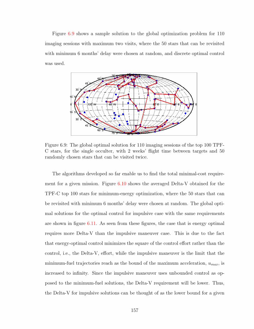
Figure 6.9 shows a sample solution to the global optimization problem for 110
imaging sessions with maximum two visits, where the 50 stars that can be revisited
with minimum 6 months’ delay were chosen at random, and discrete optimal control
was used.
Figure 6.9: The global optimal solution for 110 imaging sessions of the top 100 TPF-C stars, for the single occulter, with 2 weeks’ flight time between targets and 50randomly chosen stars that can be visited twice.
The algorithms developed so far enable us to find the total minimal-cost require-
ment for a given mission. Figure 6.10 shows the averaged Delta-V obtained for the
TPF-C top 100 stars for minimum-energy optimization, where the 50 stars that can
be revisited with minimum 6 months’ delay were chosen at random. The global opti-
mal solutions for the optimal control for impulsive case with the same requirements
are shown in figure 6.11. As seen from these figures, the case that is energy optimal
requires more Delta-V than the impulsive maneuver case. This is due to the fact
that energy-optimal control minimizes the square of the control effort rather than the
control, i.e., the Delta-V, effort, while the impulsive maneuver is the limit that the
minimum-fuel trajectories reach as the bound of the maximum acceleration, umax, is
increased to infinity. Since the impulsive maneuver uses unbounded control as op-
posed to the minimum-fuel solutions, the Delta-V requirement will be lower. Thus,
the Delta-V for impulsive solutions can be thought of as the lower bound for a given
157

mission scenario, making it smaller than both minimum-fuel with bounded control
input and minimum-energy control.
Figure 6.10: The global Delta-V curves for the single occulter mission with energy-optimal control (Left: ∆t = 1 week, Right: ∆t = 2 weeks).
10 20 30 40 50 60 700
500
1000
1500
2000
2500
3000
3500
4000
4500
Radius (1000 km)
Del
ta−
V (
m/s
)
50 Imaging70 Imaging90 Imaging
10 20 30 40 50 60 70200
400
600
800
1000
1200
1400
1600
1800
2000
Radius(1000 km)
Del
ta−
V (
m/s
)
50 Imaging70 Imaging90 Imaging
Figure 6.11: The global minimum Delta-V curves for the single occulter mission withimpulsive control (Left: ∆t = 1 week, Right: ∆t = 2 weeks).
In order to understand the thrust capability that is needed for a given spacecraft,
it is important to know the maximum thrust and acceleration it has to perform in
flight. Table 6.1 shows that the maximum acceleration needed for energy-optimal
control increases as the radius of the formation does. Here, the thrust is obtained by
multiplying the acceleration requirements with the mass of the SMART-1 spacecraft
that is discussed in the next section.
158
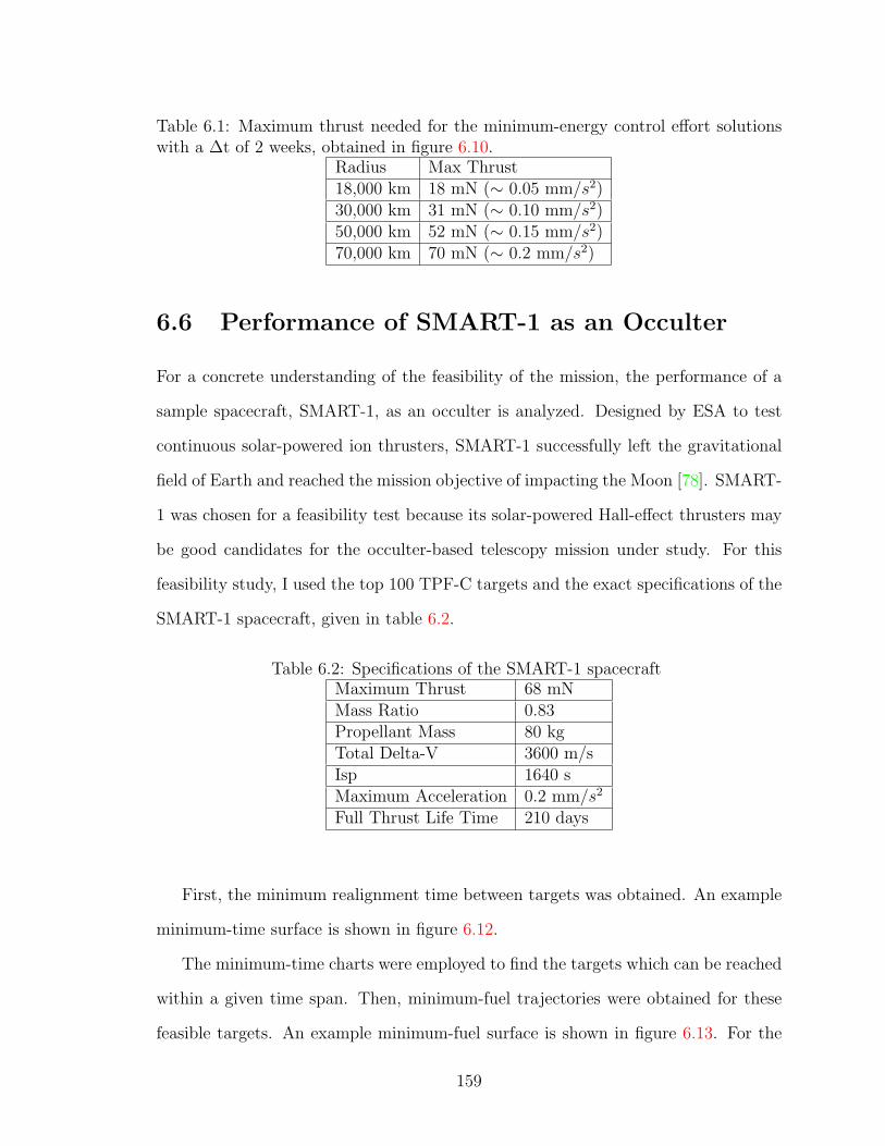
Table 6.1: Maximum thrust needed for the minimum-energy control effort solutionswith a ∆t of 2 weeks, obtained in figure 6.10.
Radius Max Thrust18,000 km 18 mN (∼ 0.05 mm/s2)30,000 km 31 mN (∼ 0.10 mm/s2)50,000 km 52 mN (∼ 0.15 mm/s2)70,000 km 70 mN (∼ 0.2 mm/s2)
6.6 Performance of SMART-1 as an Occulter
For a concrete understanding of the feasibility of the mission, the performance of a
sample spacecraft, SMART-1, as an occulter is analyzed. Designed by ESA to test
continuous solar-powered ion thrusters, SMART-1 successfully left the gravitational
field of Earth and reached the mission objective of impacting the Moon [78]. SMART-
1 was chosen for a feasibility test because its solar-powered Hall-effect thrusters may
be good candidates for the occulter-based telescopy mission under study. For this
feasibility study, I used the top 100 TPF-C targets and the exact specifications of the
SMART-1 spacecraft, given in table 6.2.
Table 6.2: Specifications of the SMART-1 spacecraftMaximum Thrust 68 mNMass Ratio 0.83Propellant Mass 80 kgTotal Delta-V 3600 m/sIsp 1640 sMaximum Acceleration 0.2 mm/s2
Full Thrust Life Time 210 days
First, the minimum realignment time between targets was obtained. An example
minimum-time surface is shown in figure 6.12.
The minimum-time charts were employed to find the targets which can be reached
within a given time span. Then, minimum-fuel trajectories were obtained for these
feasible targets. An example minimum-fuel surface is shown in figure 6.13. For the
159
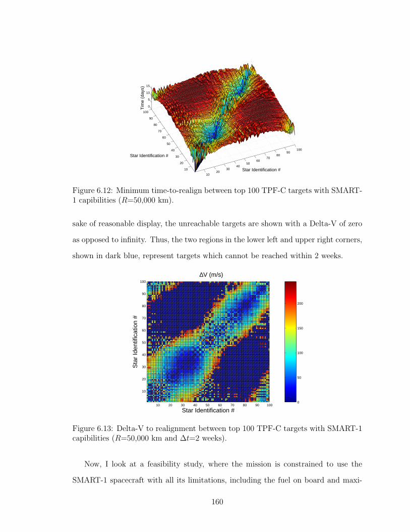
1020
3040
5060
7080
90100
10
20
30
40
50
60
70
80
90
100
0
5
10
15
Star Identification #
Star Identification #
Tim
e (d
ays)
Figure 6.12: Minimum time-to-realign between top 100 TPF-C targets with SMART-1 capibilities (R=50,000 km).
sake of reasonable display, the unreachable targets are shown with a Delta-V of zero
as opposed to infinity. Thus, the two regions in the lower left and upper right corners,
shown in dark blue, represent targets which cannot be reached within 2 weeks.
10 20 30 40 50 60 70 80 90 100
10
20
30
40
50
60
70
80
90
100
Star Identification #
Sta
r Id
entif
icat
ion
#
∆V (m/s)
0
50
100
150
200
Figure 6.13: Delta-V to realignment between top 100 TPF-C targets with SMART-1capibilities (R=50,000 km and ∆t=2 weeks).
Now, I look at a feasibility study, where the mission is constrained to use the
SMART-1 spacecraft with all its limitations, including the fuel on board and maxi-
160

mum thrust. I assume that the spacecraft continues imaging until the fuel is depleted.
Figure 6.14 shows the results that would be obtained if a minimum-fuel strategy were
employed. Since the fuel on board is limited, a more spendthrift fast slew approach,
where the time between the imaging sessions is decreased, leads to a decrease in the
total number of observations. The last data points at 20,000 km for 1 week and 70,000
km for 2 weeks are very restrictive, since they give very few options for consecutive
targets. As a result, they do not provide the flexibility that is needed in a real-life
mission.
10 20 30 40 50 60 70150
200
250
300
350
400
450
500
550
600
Radius (1000 km)
# of
Imag
ing
Ses
sion
s
2 weeks1 week
Figure 6.14: The total number of imaging sessions versus the radius, for the fuel-optimal control case (with SMART-1 capabilities).
Figure 6.15 shows the results that would be obtained if a minimum-time trans-
fer strategy were employed. This figure shows that, as the radius of the formation
increases, the total number of imaging sessions decreases. When this is compared
with figure 6.14, it is apparent that the minimum-time strategy trades off the speed
of observations against the total number of observations.
Even though the results from figures 6.14 and 6.15 should be treated as the opti-
mistic upper bounds for the number of possible imaging sessions, it is apparent that,
161
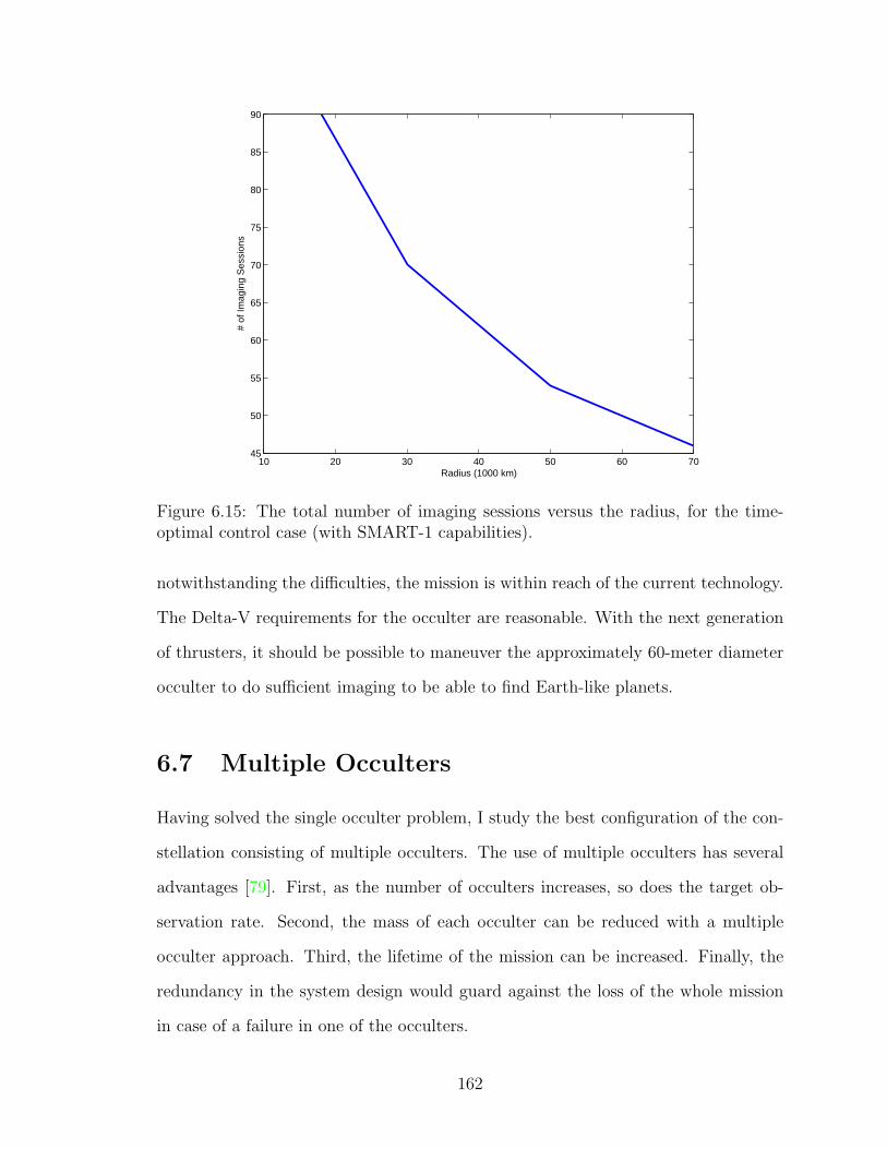
10 20 30 40 50 60 7045
50
55
60
65
70
75
80
85
90
Radius (1000 km)
# of
Imag
ing
Ses
sion
s
Figure 6.15: The total number of imaging sessions versus the radius, for the time-optimal control case (with SMART-1 capabilities).
notwithstanding the difficulties, the mission is within reach of the current technology.
The Delta-V requirements for the occulter are reasonable. With the next generation
of thrusters, it should be possible to maneuver the approximately 60-meter diameter
occulter to do sufficient imaging to be able to find Earth-like planets.
6.7 Multiple Occulters
Having solved the single occulter problem, I study the best configuration of the con-
stellation consisting of multiple occulters. The use of multiple occulters has several
advantages [79]. First, as the number of occulters increases, so does the target ob-
servation rate. Second, the mass of each occulter can be reduced with a multiple
occulter approach. Third, the lifetime of the mission can be increased. Finally, the
redundancy in the system design would guard against the loss of the whole mission
in case of a failure in one of the occulters.
162
I consider two approaches to the multiple occulter formation, in the first, the
occulters are placed on fuel-free Quasi-Halo orbits around the telescope’s Halo orbit.
This method is discussed in the first section. In the other approach, the global
optimization problem is formulated as in the single occulter case, and it is solved
using simulated annealing. This method is explored in the later sections and results
are shown. The single and the multiple occulter approaches are compared in light of
these results.
6.7.1 Multiple Occulters on Quasi-Halo Orbits
First, I consider the approach where multiple occulters are placed on Quasi-Halo
orbits around the base Halo orbit. The optimal placement problem then becomes
an optimization of the 3 × N parameters that uniquely define N Quasi-Halo orbits,
namely the size and the two-phase angles (R, θ1, θ2) of all the occulters, such that,
in the absence of any control, the occulters’ trajectories come close to intersecting
the maximum number of star LOS within a given time span. This is achieved by
first choosing points in the (R, θ1, θ2) space that define the Quasi-Halos found in the
second section, and then integrating these forward in time ( See Figure 6.16 ). The
relative motion of these orbits with respect to the base Halo orbit is transformed to
inertial coordinates; an easily reachable region, such as +5, -5 degrees from the path,
is then defined; and the number of targets that would be enclosed in this region is
found. The 3 × N parameters that give the highest number of targets in the union
are taken to be the best initial guess for the formation.
These ideas were implemented by Princeton mechanical and aerospace engineer-
ing student Azuka Chikwendu in his undergraduate thesis [80]. Looking at spacecraft
placed on multiple Quasi-Halo orbits, he showed that the two-occulter mission de-
creases the Delta-V drastically, while the addition of a third occulter is of less value
for the mission. As an example from his work, the best set of three quasi-halo orbits
163

Figure 6.16: Skyplot of the areas of the sky which are easily accessible by two differentQuasi-Halo orbits.
with 70,000 km radius around the halo orbit is shown in figure 6.17, which plots the
star coverage that would be achieved by these orbits for half of the five-year mission.
Figure 6.17: Ideal three-occulter mission, shown for 5 orbital periods, with 5 degreerange indicated [80].
6.7.2 Global Optimization with Constraints
In this section, the global optimization problem is formulated as in the single occulter
case, and it is solved using simulated annealing.
164

Mathematical Model
The full formulation for the mathematical model for the case with two occulters,
maximum two visits and no revisit of the same star with the same occulter, can be
written as:
Min∑i,j
c(i, j, ui) xij + c(i, j, vi) yij
s. t.∑
i
xij = 1,∑
i
yij = 1 ∀ j 6= i
∑j
xij = 1,∑
j
yij = 1 ∀ i 6= j
xij ∈ 0, 1, yij ∈ 0, 1 ∀ i, j
u1 = 1, v1 = 1
2 6 ui 6 n, 2 6 vi 6 n ∀ i 6= 1
ui − uj + 1 6 (n− 1)(1− xij), vi − vj + 1 6 (n− 1)(1− yij) ∀ i 6= 1, j 6= 1
Nrevisit 6 abs(vi − ui) ∀ i , (6.13)
where xij and yij are 1 if arc(i,j) is in the tour of the first and second occulter,
respectively, and ui and vi are the positions of the ith target in the first and second
occulters tour. The cost matrix, c, is the same as in the single occulter case. Without
loss of generality, u1 and v1 can be set to different starting target stars. The more
complicated case, where the same occulter is allowed to image the same star more
than once, is not included in this dissertation.
Numerical Method: Simulated Annealing
I proceed as in the single occulter case, using simulated annealing to this time solve the
two-occulter global optimization. The results can be easily extended for formations
with more than two occulters.
165
First, I define X, the vector which contains the visiting sequence of each star, as
well as the visiting partner, if they exist. However, this time, X includes the sequence
for two occulters. The odd elements of X refer to the identification number of the
star that is being imaged at that time by the first occulter, and the even elements
refer to that of the second occulter. The time interval between each imaging is fixed.
The telescope first images star X(1) using the first occulter. After time ∆t, it images
star X(2) using the second occulter, and then, after ∆t, it images star X(3) using the
first occulter, and so on.
For the constants in the algorithm, a cooling constant of ∼0.99-0.999 and an
initial temperature of approximately 100 degrees gave good results. I set the freezing
temperature to be one degree.
I used the same three-dimensional cost matrix, c, as is in the single occulter
simulated annealing algorithm. As for the functions, since even and odd elements
of X, the visiting sequence vector, define different occulters, the cost for the total
mission is the summation of the cost for each occulter. This can be expressed as
min∑
k
c(X(k), X(k + 2), k) . (6.14)
Here, for summation over odd values of i, the cost associated with the first occulter
is obtained, while for summation over even values of i, the cost associated with the
second occulter is found.
I used the same neighbor function as in the single occulter case. The random
swap and mutations are kept the same, with the single difference that the swapping
of the consecutive imaging sessions is now equivalent to swap(X(k), X(k+2)) instead
of swap(X(k), X(k+1)).
166
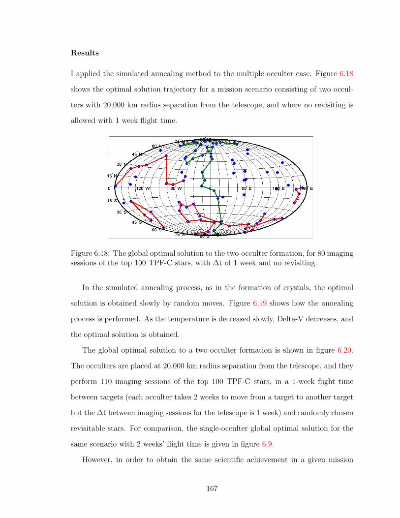
Results
I applied the simulated annealing method to the multiple occulter case. Figure 6.18
shows the optimal solution trajectory for a mission scenario consisting of two occul-
ters with 20,000 km radius separation from the telescope, and where no revisiting is
allowed with 1 week flight time.
Figure 6.18: The global optimal solution to the two-occulter formation, for 80 imagingsessions of the top 100 TPF-C stars, with ∆t of 1 week and no revisiting.
In the simulated annealing process, as in the formation of crystals, the optimal
solution is obtained slowly by random moves. Figure 6.19 shows how the annealing
process is performed. As the temperature is decreased slowly, Delta-V decreases, and
the optimal solution is obtained.
The global optimal solution to a two-occulter formation is shown in figure 6.20.
The occulters are placed at 20,000 km radius separation from the telescope, and they
perform 110 imaging sessions of the top 100 TPF-C stars, in a 1-week flight time
between targets (each occulter takes 2 weeks to move from a target to another target
but the ∆t between imaging sessions for the telescope is 1 week) and randomly chosen
revisitable stars. For comparison, the single-occulter global optimal solution for the
same scenario with 2 weeks’ flight time is given in figure 6.9.
However, in order to obtain the same scientific achievement in a given mission
167
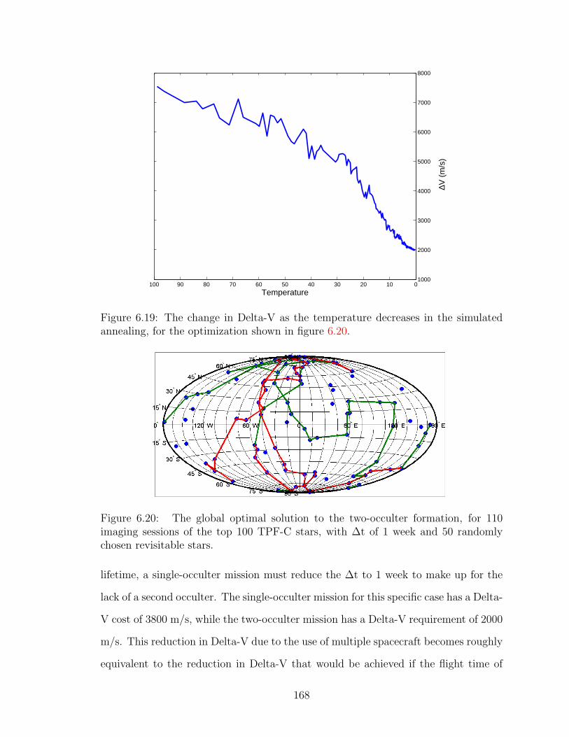
01020304050607080901001000
2000
3000
4000
5000
6000
7000
8000
Temperature
∆V (
m/s
)
Figure 6.19: The change in Delta-V as the temperature decreases in the simulatedannealing, for the optimization shown in figure 6.20.
Figure 6.20: The global optimal solution to the two-occulter formation, for 110imaging sessions of the top 100 TPF-C stars, with ∆t of 1 week and 50 randomlychosen revisitable stars.
lifetime, a single-occulter mission must reduce the ∆t to 1 week to make up for the
lack of a second occulter. The single-occulter mission for this specific case has a Delta-
V cost of 3800 m/s, while the two-occulter mission has a Delta-V requirement of 2000
m/s. This reduction in Delta-V due to the use of multiple spacecraft becomes roughly
equivalent to the reduction in Delta-V that would be achieved if the flight time of
168
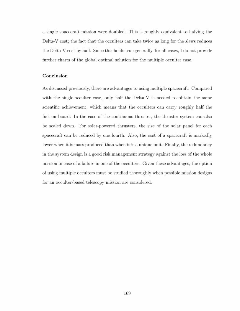
a single spacecraft mission were doubled. This is roughly equivalent to halving the
Delta-V cost; the fact that the occulters can take twice as long for the slews reduces
the Delta-V cost by half. Since this holds true generally, for all cases, I do not provide
further charts of the global optimal solution for the multiple occulter case.
Conclusion
As discussed previously, there are advantages to using multiple spacecraft. Compared
with the single-occulter case, only half the Delta-V is needed to obtain the same
scientific achievement, which means that the occulters can carry roughly half the
fuel on board. In the case of the continuous thruster, the thruster system can also
be scaled down. For solar-powered thrusters, the size of the solar panel for each
spacecraft can be reduced by one fourth. Also, the cost of a spacecraft is markedly
lower when it is mass produced than when it is a unique unit. Finally, the redundancy
in the system design is a good risk management strategy against the loss of the whole
mission in case of a failure in one of the occulters. Given these advantages, the option
of using multiple occulters must be studied thoroughly when possible mission designs
for an occulter-based telescopy mission are considered.
169

Chapter 7
Conclusion
170
A methodology to find the optimal configuration of satellite formations consisting
of a telescope and multiple occulters around Sun-Earth L2 Halo orbits was outlined.
The dynamics around L2 was examined with a focus on the Quasi-Halo orbits which
are of interest for occulter placement. A new fully numerical method which employs
multiple Poincare sections to find quasi-periodic orbits around L2 was developed. Tra-
jectory optimization of the occulter motion between imaging sessions of different stars
was performed. The global optimization problem was solved for missions consisting
of a telescope and a single occulter employing heuristic methods. Then, these results
are extended to perform the global optimization for the multiple-occulter formation.
This dissertation introduced a baseline optimal mission design for the occulter-based
imaging mission, and enables a trade-off study comparing different occulter-based
approaches with one another as well as with their alternatives.
171

Bibliography
[1] http://planetquest.jpl.nasa.gov/TPF/tpf_index.cfm, 2008. TPF website.
[2] Robert J. Vanderbei, David N. Spergel, and N. Jeremy Kasdin. Circularly sym-
metric apodization via starshaped masks. Astrophysical Journal, 599:686, 2003.
[3] Robert J. Vanderbei, David N. Spergel, and N. Jeremy Kasdin. Spiderweb masks
for high-contrast imaging. Astrophysical Journal, 590:593, 2003.
[4] D. G. Koch, W. Borucki, E. Dunham, J. Geary, R. Gilliland, J. Jenkins,
D. Latham, E. Bachtell, D. Berry, W. Deininger, R. Duren, T. N. Gautier,
L. Gillis, D. Mayer, C. D. Miller, D. Shafer, C. K. Sobeck, C. Stewart, and
M. Weiss. Overview and status of the Kepler Mission. In J. C. Mather, edi-
tor, Optical, Infrared, and Millimeter Space Telescopes. Edited by Mather, John
C. Proceedings of the SPIE, Volume 5487, pp. 1491-1500 (2004)., volume 5487
of Presented at the Society of Photo-Optical Instrumentation Engineers (SPIE)
Conference, pages 1491–1500, October 2004.
[5] R. Goullioud, J. H. Catanzarite, F. G. Dekens, M. Shao, and J. C. Marr, IV.
Overview of the SIM PlanetQuest Light (SIM-Lite) mission concept. ArXiv e-
prints, 807, July 2008.
[6] http://www.kepler.arc.nasa.gov/PageMill_Resources/Disc_sp.gif,
2007. NASA Kepler Mission Website.
172
[7] M. Mayor and D. Queloz. A Jupiter-Mass Companion to a Solar-Type Star.
Nature, 378:355–+, November 1995.
[8] N. J. Woolf, P. S. Smith, W. A. Traub, and K. W. Jucks. The Spectrum of
Earthshine: A Pale Blue Dot Observed from the Ground. Astrophysical Journal,
574:430–433, Jul 2002.
[9] W. Cash, J. Kasdin, S. Seager, and J. Arenberg. Direct studies of exo-planets
with the New Worlds Observer. In H. A. MacEwen, editor, UV/Optical/IR
Space Telescopes: Innovative Technologies and Concepts II. Edited by MacEwen,
Howard A. Proceedings of the SPIE, Volume 5899, pp. 274-285 (2005)., volume
5899 of Presented at the Society of Photo-Optical Instrumentation Engineers
(SPIE) Conference, pages 274–285, August 2005.
[10] W. Cash, E. Schindhelm, J. Arenberg, R. Polidan, S. Kilston, and C. Noecker.
The New Worlds Observer: using occulters to directly observe planets. In Space
Telescopes and Instrumentation I: Optical, Infrared, and Millimeter. Edited by
Mather, John C.; MacEwen, Howard A.; de Graauw, Mattheus W. M.. Proceed-
ings of the SPIE, Volume 6265, pp. 62651V (2006)., volume 6265 of Presented
at the Society of Photo-Optical Instrumentation Engineers (SPIE) Conference,
Jul 2006.
[11] D. J. Des Marais, M. O. Harwit, K. W. Jucks, J. F. Kasting, D. N. C. Lin, J. I.
Lunine, J. Schneider, S. Seager, W. A. Traub, and N. J. Woolf. Remote Sens-
ing of Planetary Properties and Biosignatures on Extrasolar Terrestrial Planets.
Astrobiology, 2:153–181, June 2002.
[12] Bernard Lyot. La couronne solaire etudiee en dehors des eclipses. C. R. Hebd.
Seances Acad. Sci., 191:834–837, 1930.
173
[13] http://planetquest.jpl.nasa.gov/TPF/tpf_index.cfm, 2008. NASA Ter-
restrial Planet Finder Website.
[14] A. Give’on, N. J. Kasdin, R. J. Vanderbei, and Y. Avitzour. High-frequency
folding and optimal phase conjugation for high-contrast adaptive optics. In
D. Bonaccini Calia, B. L. Ellerbroek, and R. Ragazzoni, editors, Advancements in
Adaptive Optics. Edited by Domenico B. Calia, Brent L. Ellerbroek, and Roberto
Ragazzoni. Proceedings of the SPIE, Volume 5490, pp. 1438-1449 (2004)., vol-
ume 5490 of Presented at the Society of Photo-Optical Instrumentation Engineers
(SPIE) Conference, pages 1438–1449, October 2004.
[15] L. Pueyo and J. Kasdin. Performance Study Of Integrated Coronograph-adaptive
Optics Designs. In Bulletin of the American Astronomical Society, volume 38 of
Bulletin of the American Astronomical Society, pages 788–+, December 2007.
[16] W. Cash. Detection of earth-like planets around nearby stars using a petal
shaped occulter. Nature, (442):51–53, July 2006.
[17] R.W. Farquhar. A Halo–Orbit Lunar Station. Astronautics and Aeronautics,
10(6):59–63, 1972.
[18] R.W. Farquhar, D.P. Muhonen, C. Newman, and H. Heuberger. The First Li-
bration Point Satellite. Mission Overview and Flight History. In AAS/AIAA
Astrodynamics Specialist Conference, 1979.
[19] R.W. Farquhar and D.W. Dunham. Libration–Point Staging Concepts for Earth–
Mars Transportation. Technical Report M002, NASA, 1986.
[20] R.W. Farquhar and D.W. Dunham. Use of Libration–Point Orbits for Space
Observatories. In Observatories in Earth Orbits and Beyond, Ed by Y. Kondo,
Kluwer Academic Publishers, pages 391–395, 1990.
174

[21] R.B. Bate, D.D. Mueller, and J.E. White. Fundamentals of Astrodynamics. Dover
Publications, 1971.
[22] R.H. Battin. An Introduction to the Mathematics and Methods of Astrodynamics.
AIAA Education Series, 1987.
[23] H. Goldstein, C. Poole, and J. Safko. Classical Mechanics. Addison Wesley, 3
edition, 2001.
[24] V. Szebehely. Theory of Orbits: The Restricted Problem of the Three Bodies.
Academic Press, New York, 1967.
[25] G. Gomez, W. S. Koon, M. W. Lo, J. E. Marsden, J. Masdemont, and S. D. Ross.
Connecting orbits and invariant manifolds in the spatial restricted three-body
problem. Nonlinearity, 17:1571–1606, September 2004.
[26] http://upload.wikimedia.org/wikipedia/commons/b/b8/Lagrange_very_
massive.svg, 2008. Lagrange Point Figure.
[27] D.L. Richardson. Analytical Construction of Periodic Orbits About the Collinear
Points. Celestial Mechanics, 22(3):241–253, 1980.
[28] W.S. Koon, M.W. Lo, J.E. Marsden, and S.D. Ross. Heteroclinic Connections Be-
tween Periodic Orbits and Resonance Transitions in Celestial Mechanics. Chaos,
10(2):427–469, 2000.
[29] W. S. Koon, M.W. Lo, J.E. Marsden, and S.D. Ross. The genesis trajectory and
heteroclinic connections. AAS, 103(3):2327–2343, 1999. AAS 99-451.
[30] J.L. Bell et al. Genesis Trajectory Design. Advances in the Astronautical Sci-
ences, 103:1525–1537, 2000.
[31] R.W. Farquhar. Lunar Communications with Libration–Point Satellites. Journal
of Spacecraft and Rockets, 4(10):1383–1384, 1967.
175
[32] R.W. Farquhar. Station–Keeping in the Vicinity of Collinear Libration Points
with an Application to a Lunar Communications Problem. In Space Flight Me-
chanics, Science and Technology Series, volume 11, pages 519–535. American
Astronautical Society, New York, 1967.
[33] R.W. Farquhar. Future Missions for Libration–Point Satellites. Astronautics &
Aeronautics, 7(5):52–56, 1969.
[34] G. Gomez, J. Llibre, R. Martınez, and C. Simo. Dynamics and Mission Design
Near Libration Point Orbits – Volume 2: Fundamentals: The Case of Triangular
Libration Points. World Scientific, 2000.
[35] A. Jorba and J. Masdemont. Dynamics in the center manifold of the collinear
points of the restricted three body problem. Physica D Nonlinear Phenomena,
132:189–213, July 1999.
[36] A. Jorba and J.J. Masdemont. Dynamics in the Center Manifold of the Restricted
Three–Body Problem. Physica D, 132:189–213, 1999.
[37] K.C. Howell. Three Dimensional Periodic Halo Orbits. Celestial Mechanics,
32(1):53–72, 1984.
[38] J. R. Cash and M. H. Wright. Implementation issues in solving nonlinear equa-
tions for two-point boundary value problems. Computing, 55:17–37, 1990.
[39] J. R. Cash and M. H. Wright. A deferred correction method for nonlinear
two-point boundary value problems: Implementation and numerical evaluation.
SIAM J. Sci. Stat. Comput., 12:971–989, 1991.
[40] U. Ascher, J. Christiansen, and R. D. Russell. Collocation Software for
Boundary-Value ODEs. ACM Trans. Math Software, 7:209–222, 1981.
176

[41] U. Ascher, R. M. M. Mattheij, and R. D. Russell. Numerical Solution of Bound-
ary Value Problems for Ordinary Differential Equations. Prentice-Hall, Engle-
wood Cliffs, NJ, 1988.
[42] Jacek Kierzenka and Lawrence F. Shampine. A bvp solver based on residual
control and the maltab pse. ACM Trans. Math. Softw., 27(3):299–316, 2001.
[43] Milton Abramowitz and Irene A. Stegun. Handbook of Mathematical Functions
with Formulas, Graphs, and Mathematical Tables. Dover, New York, ninth dover
printing, tenth gpo printing edition, 1964.
[44] J. Guckenheimer and P. Holmes. Nonlinear Oscillations, Dynamical Systems,
and Bifurcations of Vector Fields. Springer-Verlag, New York, 1983.
[45] E. T. Campbell. Bifurcations from Families of Periodic Solutions in the Circular
Restricted Problem with Application to Trajectory Design. PhD thesis, Purdue
University, August 1999.
[46] G. Gomez, J.J. Masdemont, and C. Simo. Quasihalo Orbits Associated with
Libration Points. Journal of The Astronautical Sciences, 46(2):1–42, 1999.
[47] A. Jorba and J. Villanueva. Numerical Computation of Normal Forms Around
Some Periodic Orbits of the Restricted Three Body Problem. Physica D, 114:197–
229, 1998.
[48] R. M. M. Mattheij and G. W. M. Staarink. An efficient algorithm for solving
general linear two-point bvp. SIAM J. Sci. Stat. Comp., 5:87–14, 1984.
[49] E. Kolemen, N. J. Kasdin, and P. Gurfil. Quasi-Periodic Orbits of the Restricted
Three-Body Problem Made Easy. In New Trends in Astrodynamics and Applica-
tions III, volume 886 of American Institute of Physics Conference Series, pages
68–77, Feb 2007.
177

[50] I. G. Kevrekidis, R. Aris, L. D. Schmidt, and S. Pelikan. Numerical computations
of invariant circles of maps. Physica D, 16:243–251, 1985.
[51] http://en.wikibooks.org/wiki/Image:Polar_coordinates_integration_
region.svg, 2008. Integration in Polar Coordinates Figure.
[52] Marc-Antoine Parseval des Chenes. Memoire sur les series et sur l’intgration
complete d’une equation aux differences partielle lineaire du second ordre, a coef-
ficiens constans. Memoires presentes a lInstitut des Sciences, Lettres et Arts, par
divers savans, et lus dans ses assemblees. Sciences, mathmatiques et physiques.,
1:638–648, 1806.
[53] J. R. Dormand and P. J. Prince. High order embedded runge-kutta formulae. J.
Comp. Appl. Math., 7(1):67–75, 1981.
[54] C. Runge. Uber empirische funktionen und die interpolation zwischen
aquidistanten ordinaten. Zeitschrift fur Mathematik und Physik, 46:224–243,
1901.
[55] G. Gomez and J. M. Mondelo. The dynamics around the collinear equilibrium
points of the rtbp. Physica D, 157(4):283–321, October 2001.
[56] J. M. Mondelo. Contribution to the Study of Fourier Methods for Quasi-Periodic
Functions and the Vicinity of the Collinear Libration Points. PhD thesis, Uni-
versitat de Barcelona, Departament de Matematica Aplicada i Analisi, 2001.
[57] E.M. Standish. Jpl planetary and lunar ephemerides, de405/le405. JPL IOM,
312.F-98-048, 1998.
[58] E.M. Standish Jr. Orientation of the jpl ephemerides, de200/le200, to the dy-
namical equinox of j 2000. Astron. Astrophys., 114:297–302, 1982.
[59] http://sco.stsci.edu/roses/index.php, 2007. Top 100 TPF-C Targets.
178

[60] M. A. C. Perryman, L. Lindegren, J. Kovalevsky, E. Hoeg, U. Bastian, P. L.
Bernacca, M. Creze, F. Donati, M. Grenon, F. van Leeuwen, H. van der Marel,
F. Mignard, C. A. Murray, R. S. Le Poole, H. Schrijver, C. Turon, F. Arenou,
M. Froeschle, and C. S. Petersen. The HIPPARCOS Catalogue. Astronomy and
Astrophysics, 323:L49–L52, July 1997.
[61] G. H. Kaplan, J. A. Hughes, P. K. Seidelmann, C. A. Smith, and B. D. Yallop.
Mean and apparent place computations in the new IAU system. III - Apparent,
topocentric, and astrometric places of planets and stars. Astronomical Journal,
97:1197–1210, April 1989.
[62] R. F. Stengel. Optimal Control and Estimation. Dover, New York, 1994.
[63] A. E. Bryson and Y. C. Ho. Applied Optimal Control. Hemisphere Publishing
Corp., New York, 1975.
[64] J. T. Betts. Practical Methods for Optimal Control using Nonlinear Program-
ming. SIAM, Philadelphia, 2001.
[65] Margaret H. Wright Philip E. Gill, Walter Murray. Practical Optimization. Aca-
demic Press, 1982.
[66] A. Wachter and L. T. Biegler. Line search filter methods for nonlinear pro-
gramming: Motivation and global convergence. SIAM Journal on Optimization,
16(1):1–31, 2005.
[67] http://www.mathworks.com/support/tech-notes/1600/1605.html, 2008.
Online manual for MATLAB’s mex function.
[68] Donald E. Kirk. Optimal Control Theory: An Introduction. Prentice-Hall, En-
glewood Cliffs, NJ, 1970.
179

[69] Paul Leopardi. A partition of the unit sphere into regions of equal area and small
diameter. Electronic Transactions on Numerical Analysis, 25:309–327, 2006.
[70] C. E. Miller, A. W. Tucker, and R. A. Zemlin. Integer programming formulation
of traveling salesman problems. Journal of the ACM, 7(4):326–329, Oct 1960.
[71] http://www.tsp.gatech.edu/concorde.html, 2008. Concorde TSP Solver.
[72] G. Gutin and A. P. Punnen, editors. Travelling Salesman Problem and Its Vari-
ations, volume 12 of Combinatorial Optimization. Kluwer Academic Publishers,
New York, 2002.
[73] F. Glover and M. Laguna. Tabu Search. Kluwer Academic Publishers, Norwell,
MA, 1997.
[74] Marco Dorigo and Luca Maria Gambardella. Ant colony system: A cooperative
learning approach to the traveling salesman problem. IEEE Transactions on
Evolutionary Computation, 1:53–66, 1997.
[75] P. T. De Boer, D. P. Kroese, S. Mannor, and R. Y. Rubinstein. A tutorial on
the cross-entropy method. Annals of Operations Research, 134, 2004.
[76] S. Kirkpatrick, C. D. Gelatt, and M. P. Vecchi. Optimization by simulated
annealing. Science, 220(4598):671–680, May 1983.
[77] http://upload.wikimedia.org/wikipedia/commons/8/85/Rundtur.GIF,
2008. 2-opt procedure.
[78] http://www.esa.int/SPECIALS/SMART-1, 2008. The official SMART-1 website.
[79] I. Jordan, H. Hart, A. Schultz, G. Starkman, C. Copi, and R. Lyon. The ad-
vantages of multiple coronagraphic vehicles in occulter missions. In Space 2003
Conference Proc., Sep 2003. AIAA-2003-6300, ISBN 1-56347-647-9.
180

[80] Azuka Chikwendu. Optimization of multiple occulter mission in quasi-halo orbit.
Princeton University, Undergraduate Thesis, 2007.
181