


1
On the global character of overlap between low and high 1 clouds 2
Tianle Yuan1,2 and Lazaros Oreopoulos1 3
1Climate and Radiation Laboratory, NASA Goddard Space Flight Center 4
2Joint Center for Environmental Technology and Department of Physics, UMBC, 5
Baltimore, MD 6
7
8
9
10
11
12
13
14
15
16
17
*Correspondence should be addressed to: Tianle Yuan, [email protected] 18
Building 33 Room A306 19
Mail code 613 20
Greenbelt, MD, 20771 21
Tel: 301-‐614-‐6195 22
Fax: 301-614-6307 23
24
25
2
Abstract 25 The global character of overlap between low and high clouds is examined using active 26
satellite sensors. Low cloud fraction has a strong land-ocean contrast with oceanic values 27
double those over land. Major low cloud regimes include not only the eastern ocean 28
boundary stratocumulus and shallow cumulus but also those associated with cold air 29
outbreaks downwind of wintertime continents and land stratus over particular geographic 30
areas. Globally, about 30% of low clouds are overlapped by high clouds. The overlap rate 31
exhibits strong spatial variability ranging from higher than 90% in the tropics to less than 32
5% in subsidence areas, and is anti-correlated with subsidence rate and low cloud 33
fraction. The zonal mean of vertical separation between cloud layers is never smaller than 34
5 km and its zonal variation closely follows that of tropopause height, implying a tight 35
connection with tropopause dynamics. Possible impacts of cloud overlap on low clouds 36
are discussed. 37
38

3
Introduction 38
Thin high clouds and low boundary layer clouds are two important cloud types in terms 39
of cloud radiative effect. Thin high clouds are ubiquitous in the atmosphere (Liou 1986; 40
Sassen et al., 2008). They trap outgoing longwave radiation and exert a net warming 41
effect since they have only a minor influence on the shortwave radiation. Low boundary 42
layer clouds on the other hand strongly modulate shortwave albedo while only weakly 43
changing the longwave radiation. They are the primary contributor to the net climate 44
cooling effect (Hartmann et al., 1992). Analysis of ISCCP data reveals that these 45
vertically well-separated cloud types often co-exist in the same geographic area, and this 46
is corroborated by observations from other sources (Jakob and Tselioudis, 2003, Mace et 47
al., 2007). In this type of high-over-low-cloud overlap, the net radiative impact of the two 48
cloud types is expected to cancel out at the top of atmosphere to some degree. 49
Furthermore, the presence of high clouds can significantly modify low cloud top 50
cooling/heating, primarily through their longwave effects, which can strongly affect low 51
cloud development (Chen and Cotton, 1987; Christensen et al. 2013). 52
53
Before the advent of space-borne active (lidar/radar) sensors this type of overlap posed a 54
challenge for passive sensors with regard to detecting the occurrence and characterizing 55
the properties of the two cloud layers. Pure infrared (IR) techniques often misidentify the 56
overlapping clouds as moderately thick mid-level clouds (Chang and Li, 2005a). The 57
CO2-slicing technique provides a good detection method for identifying isolated high 58
clouds, but in overlap situations can misidentify the two overlapped layers as a single 59
thick high cloud. While a combined usage of CO2-slicing, shortwave near IR and thermal 60
4
IR channels can offer much better performances (Baum et al., 1995, Pavolonis and 61
Heidinger, 2004, Chang and Li, 2005a, Wind et al., 2010), to unambiguously detect and 62
better characterize overlapping clouds, active sensors are a much better option as 63
demonstrated by studies of general statistics overlap and cloud vertical structure using 64
such sensors (Wang and Dessler, 2006, Mace et al., 2007). 65
66
Previous works have shown that high-low cloud overlap type is quite prevalent 67
throughout the globe (Warren et al., 1985, Tian and Curry, 1989). According to a study 68
employing a two-layer retrieval technique on MODIS data (Chang and Li, 2005b) low 69
clouds are overlapped by thin high clouds at a rate of 43% over land and 36% over ocean. 70
Another survey with space-borne lidar data shows that this type of overlap is the most 71
frequent overlap type and about 32% of all low tropical clouds are overlapped by high 72
cloud above (Wang and Dessler, 2006). 73
74
Investigations on the origin of high-over-low-cloud overlap, its dynamic control and 75
large-scale variations have been lacking. Here we use data from CloudSat and Cloud-76
Aerosol Lidar and Infrared Pathfinder Satellite Observations (CALIPSO) in conjunction 77
with NASA Modern Era Retrospective-Analysis for Research and Applications 78
(MERRA; Rienecker et al., 2011) reanalysis data to shed more light on certain aspects of 79
this overlap. 80
Data and method 81
The CloudSat cloud profiling radar (CPR) is a 94 GHz nadir-looking radar, which records 82
reflectivity from hydrometeors at effectively 250 m vertical and 1.5 km along-track 83

5
resolutions (Marchand et al., 2008). It has a sensitivity of about -30 dBZ and can 84
penetrate most cloud layers except those that are heavily precipitating. The Cloud-85
Aerosol Lidar with Orthogonal Polarization (CALIOP) is aboard CALIPSO which is part 86
of the A-Train constellation along with CloudSat. CALIOP is a two-wavelength 87
polarization-sensitive lidar that measures cloud and aerosols at a 333 m horizontal and 88
30-60 m vertical resolutions with a maximum penetration optical depth of about 3. Two 89
different data sets are employed in this study. The main data set is the CloudSat-90
CALIPSO combined 2B-GEOPROF-Lidar product (Mace et al., 2009). The other is the 91
CALIOP 1-km cloud layer product that reports the occurrence of cloud layers using only 92
the lidar signal (Vaughan et al., 2004). The CALIOP only product will likely miss 93
overlaps when high clouds are sufficiently thick, while CloudSat CPR can penetrate 94
moderately thick clouds and still detect low clouds above 1km (Marchand et al., 2008). 95
The combined product therefore represents the best space-borne data source for our 96
purposes despite occasional underestimates of low cloud fraction by the CPR (Mace et 97
al., 2007, Mace et al., 2009). 98
99
Low clouds are defined here as having tops up to 3.5 km above the local topography or 100
sea level, which is similar to the threshold of 680 hPa in previous studies (Rossow and 101
Schiffer, 1999) except over highlands. The high clouds in this study are defined as having 102
cloud base higher than 5 km relative to the local topography or higher than 7 km above 103
sea level. When trying different thresholds to define low and high cloud layers we find 104
little sensitivity to threshold choice probably due to the well-known minimum of mid-105
level cloud occurrence (Zuidema, 1998; Chang and Li, 2005b). 106
6
107
Low clouds occur throughout the tropics, subtropics and mid-latitudes. We set our study 108
region between 60S and 60N to include different low cloud regimes. We first search for 109
low cloud presence in the lidar/radar column and if a low cloud is found, a search for 110
high clouds is conducted in the same column. From these profile-by-profile scans the 111
occurrence of non-overlapped low clouds, high-over-low-clouds, and all other situations 112
can be aggregated in 2.5° grid cells. Along with the total number of observations, 113
statistics such as monthly gridded total cloud fraction, low cloud fraction and overlap rate 114
are calculated. The NASA MERRA re-analysis data are re-sampled to the same spatial 115
grid to provide dynamic and thermodynamic context. We analyze data from January, 116
April, July and October of 2009 for both the CALIPSO 1 km-cloud layer and the 2B-117
GEOPROF-LIDAR products, in order to characterize the full seasonal cycle. 118
Unfortunately, due to the sun-synchronous orbits of the CALIPSO and CloudSat 119
satellites, the diurnal characteristics of our cloud and overlap statistics cannot be 120
resolved. 121
Results and Discussion 122
a. Low cloud cover and its regimes 123
The analysis of the 2B-GEOPROF-LIDAR product reveals that low clouds prefer ocean 124
over land. Mean low cloud fraction in oceanic gridcells, defined to be at least 80% 125
covered by water is 44% while it is 23% over land (all other gridcells). Land low cloud 126
fraction exceeds 40% over only two areas [Figure 1E], one in northern Europe 127
surrounding the Baltic Sea and the other in the vicinity of southeast China. Values over 128
northeastern Canada are also close to 40%. The common dynamic and thermodynamic 129

7
conditions in these areas include a stable lower troposphere, moderate large-scale 130
subsidence and plentiful moisture flux from adjacent water surfaces as indicated by 131
MERRA data (not shown here). While previous work has identified Southeast China as a 132
region where semi-permanent stratus clouds are prevalent (Klein and Hartmann, 1993) 133
[Figure 1A], North Europe and Northeast Canada have not been identified as such 134
regions. Given that typical cloud fraction of low-level cumulus is less than 30% 135
(Medeiros et al., 2010), dominant cloud types over North Europe [Figure 1B] and 136
Northeast Canada are likely stratus or fog. 137
138
Almost everywhere, low-cloud fraction over other land areas is less than 30%, which 139
suggests either a regime change from stratus to fair-weather cumulus or more obscuration 140
occurrences. Unobscured marine low cloud fraction reaches minima throughout the deep 141
tropics and maxima in major stratocumulus dominated areas [e.g. Figure 1C] and mid-142
latitude storm track regions. Peak cloud fraction ranges from 80% in January and April to 143
close to 100% in October and July and occurs exclusively in the eastern ocean boundary 144
stratocumulus regime. Cloud fractions in trade cumulus dominated regions are much 145
lower by comparison. Less attention has been paid to a regime of low clouds associated 146
with cold air outbreaks in the winter season downwind of major continents (Atkinson and 147
Zhang, 1996)[Figure 1D]. These are formed when strong winds associated with cold air 148
mass pick up moisture and heat from warm oceanic currents, creating favorable 149
conditions for low cloud formation (Young and Kristovich, 2002). These clouds appear 150
as “streets” with embedded closed cell stratocumulus [Figure 1D] and are responsible for 151
local winter-time cloud fraction maxima east of the coasts of China, Japan, East Siberia 152

8
and North America [Figure 1D]. This cloud regime does not appear as often in the part of 153
the southern hemisphere we consider for this analysis mostly because of the absence of 154
the strong land-ocean temperature contrast encountered at northern mid-latitudes. 155
b. High-over-low-cloud overlap 156
The global mean overlap rate, defined as the ratio of the number of profiles with overlap 157
to the number of low cloud profiles, is 30% in January 2009, with slightly higher values 158
over land (32.6%) than over ocean (28.5%). However, it exhibits large spatial variations 159
that are associated with clearly identifiable regimes. Maxima are reached in the tropical 160
convective areas, in particular the Pacific Warm Pool and surrounding maritime 161
continents where overlap rates of 80% are common. Over these areas low clouds can only 162
be detected in-between convective events. Due to the ubiquitous presence of cirrus clouds 163
from either large-scale ascent or from dissipating deep convection, it is highly likely that 164
a detected low cloud will be found overlapped by cirrus although overall low cloud 165
fraction is low in these areas (Figure 1). Minima are generally found over some land 166
areas and over major stratocumulus dominated oceanic areas, where values can drop 167
below 5%. These are regions of persistent strong subsidence, generally unfavorable for 168
upper level cloud formation. However, we note that even within this regime there are 169
substantial seasonal and spatial variations and off the coast of California it can reach up 170
to 15-25%. The source of high cloud in these areas is mainly topography-driven gravity 171
wave activity, advection from neighboring tropical convection centers such as Amazon 172
Basin, Congo Basin, or ascent associated with mid-latitude fronts. Intermediate values 173
range from 35% to 65% in the mid-latitude storm track regions in accordance with recent 174
findings of thin cirrus prevalence in cyclonic systems (Posselt et al., 2008, Sassen et al., 175
9
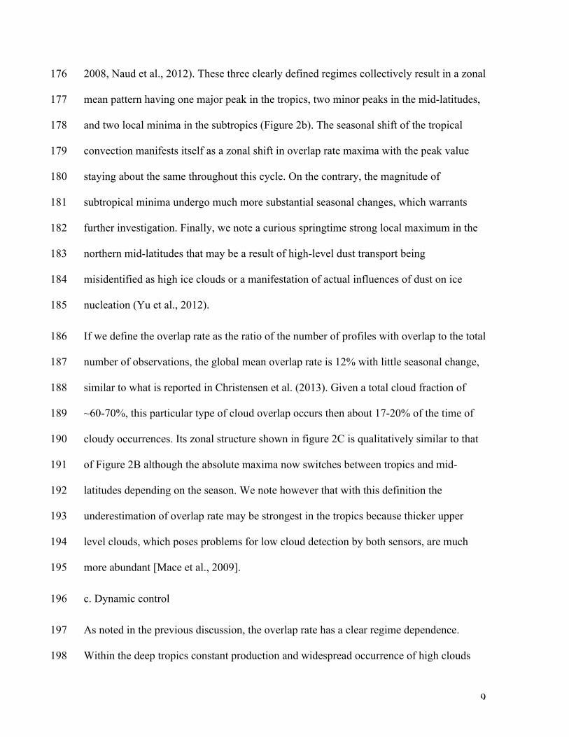
2008, Naud et al., 2012). These three clearly defined regimes collectively result in a zonal 176
mean pattern having one major peak in the tropics, two minor peaks in the mid-latitudes, 177
and two local minima in the subtropics (Figure 2b). The seasonal shift of the tropical 178
convection manifests itself as a zonal shift in overlap rate maxima with the peak value 179
staying about the same throughout this cycle. On the contrary, the magnitude of 180
subtropical minima undergo much more substantial seasonal changes, which warrants 181
further investigation. Finally, we note a curious springtime strong local maximum in the 182
northern mid-latitudes that may be a result of high-level dust transport being 183
misidentified as high ice clouds or a manifestation of actual influences of dust on ice 184
nucleation (Yu et al., 2012). 185
If we define the overlap rate as the ratio of the number of profiles with overlap to the total 186
number of observations, the global mean overlap rate is 12% with little seasonal change, 187
similar to what is reported in Christensen et al. (2013). Given a total cloud fraction of 188
~60-70%, this particular type of cloud overlap occurs then about 17-20% of the time of 189
cloudy occurrences. Its zonal structure shown in figure 2C is qualitatively similar to that 190
of Figure 2B although the absolute maxima now switches between tropics and mid-191
latitudes depending on the season. We note however that with this definition the 192
underestimation of overlap rate may be strongest in the tropics because thicker upper 193
level clouds, which poses problems for low cloud detection by both sensors, are much 194
more abundant [Mace et al., 2009]. 195
c. Dynamic control 196
As noted in the previous discussion, the overlap rate has a clear regime dependence. 197
Within the deep tropics constant production and widespread occurrence of high clouds 198

10
makes high-over-low-cloud overlap highly likely whenever a low cloud is present. Gentle 199
large-scale ascent and ice cloud production from frontal convection are likely responsible 200
for the local maximum in the mid-latitude storm tracks. The strong and deep subsidence 201
layer over the subtropical stratocumulus regions suppresses local production of ice clouds 202
and reduces the overlap to a minimum. Here, we use MERRA monthly pressure vertical 203
velocity data at 500 hPa (Omega500) and 700 hPa (Omega700) as a proxy for dynamic 204
regimes and investigate the relationship between the overlap rate and the dynamic 205
condition. 206
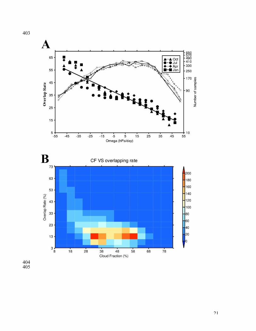
We find good anti-correlation between Omega700 (or Omega500) and the monthly 207
gridded overlap rate (correlation coefficient r = -0.94, and probability of the null 208
hypothesis p<0.001) over the ocean. The frequency distribution of Omega700 is 209
negatively skewed and to include sufficient samples for each bin we limit our calculation 210
within the range of -50 to 50 hPa/day. Overlap rate data are averaged within 5 hPa/day 211
bins. The overlap rate increases with decreasing Omega700 at a rate of about 0.45 212
percent/hPa and the intercept with zero vertical velocity is around 35%. Scaling is found 213
for all months examined with similar slope and intercept. A similar relationship is found 214
if Omega500 is used and is therefore not shown here. Qualitatively, the correlation is 215
expected because of the clearly defined cloud system regimes and the vertical velocity 216
associated with them. However, existence of such a robust quantitative scaling is not 217
trivial. The slope and intercept of this linear relationship are not sensitive to seasonal 218
changes, which makes it a useful constraint for diagnosing model performances of this 219
type of overlap occurrence. When the alternate overlap rate definition of Figure 2C is 220
11
used, a similar anti-correlation with Omega700 and Omega500 is found (results not 221
shown here). 222
An anti-correlation (r= -0.56, p<0.001) exists between low cloud fraction and overlap rate 223
over the ocean (Figure 3b). This is easily understood because the strong subsidence 224
favors low cloud formation and suppresses ice cloud generation. However, the fact that 225
these two cloud types can still co-exist under this condition makes this type of overlap 226
challenging and interesting to represent in models. Topographically and convectively 227
generated gravity waves are likely candidates for generating high clouds in these large-228
scale subsidence regions. 229
d. Vertical separation 230
Our definitions require that high clouds have bases either 5 km above local topography or 231
7 km above sea level and that the top of low clouds is below 3.5 km above the local 232
topography or sea level. These definitions of high and low clouds do not in principle 233
restrict their vertical separation to large values. Our dataset indicates (Figure 4a) that the 234
vertical separation between the two cloud layers has a clear zonal dependence, but is 235
never smaller than 5 km in the zonal mean, highlighting the absence of mid-level clouds 236
and the well-separated nature of these cloud types. The height difference reaches 237
maximum in the tropics while it falls to a minimum over highland areas such as the 238
Himalayas, the Iranian Plateau and the Rocky Mountains. These minima are due in a 239
large part to the high ground elevation. Since low cloud top heights do not exhibit 240
systematic zonal variations (figure not shown) most of the zonal structure in vertical 241
separation comes from zonal variations of high cloud altitude which should be closely 242
related to the thermodynamic structure of the upper atmosphere. In fact the strong 243

12
latitudinal dependence of the height difference (Figure 4b) follows closely the zonal 244
structure of tropopause height (Schmidt et al., 2010). The vertical separation decreases 245
from 11 km in the tropics to around 5 km at higher latitudes. The 6 km difference is 246
similar to the tropopause height variations between the tropics and high latitudes (~60 S 247
and N) and the overall zonal structures of these two are quite similar (Schmidt et al., 248
2010). There is also a clear seasonal cycle in the magnitude of vertical separation 249
between two cloud layers. This seasonal cycle is stronger in the Northern Hemisphere 250
than that in the Southern Hemisphere, similar to the seasonal cycle of tropopause height 251
(Schmidt et al., 2010; Li et al., A global survey of the linkages between cloud vertical 252
structure and large-scale climate, submitted to JGR, 2013). We therefore believe that only 253
few mid-level clouds overlap with low clouds and the variations in height of upper-level 254
clouds are strongly tied to tropopause dynamics. 255
e. Discussion 256
The well-separated nature of the overlap makes feasible the application of dual cloud 257
layer retrievals with passive sensors (Chang and Li, 2005b, Minnis et al., 2007). It also 258
points to the potential radiative impact of this cloud overlap, especially in the longwave 259
when high cloud is thin. It is expected that the radiative interactions between the two 260
cloud layers will have implications for the evolution of both cloud types, but especially of 261
low clouds. We plan to comprehensively assess these radiative interactions and their 262
impact in a separate study. Our preliminary results suggest significant changes in both the 263
mean and diurnal cycle of low cloud properties such as cloud fraction, liquid water path, 264
precipitation and even organization (Chen and Cotton, 1987; Wang et al., 2010; 265
Christensen et al., 2013) due to the presence of high clouds aloft. 266

13
Summary 267
Active space-borne sensors are used to study the specific case of overlap between high 268
and low clouds. The low cloud fraction distribution captured by the combined radar-lidar 269
data agrees with previous work, but additional new insights are gained. Three distinct 270
overlapping regimes are identified to be associated with tropical convection, mid-latitude 271
storms and remote/local gravity wave generated high clouds over subsidence regions. The 272
overlap rate decreases in that order, in accordance with our qualitative understanding of 273
dynamics associated with each regime. Globally, 30% of low clouds are overlapped by 274
high clouds aloft. This accounts for 12% of total observations. Large-scale pressure 275
vertical velocity is found to anti-correlate well with the overlap rate through out the year. 276
The high and low layers are well separated vertically with the zonal mean of the vertical 277
separation being always greater than 5 km, exposing thus the scarcity of mid-level 278
clouds. The zonal structure of the vertical separation between the two cloud layers and its 279
seasonal cycle follow closely those of tropopause height, which may be indicative of high 280
clouds being strongly coupled with tropopause dynamics. 281
282
Acknowledgement: 283
The authors acknowledge funding support from NASA’s CALIPSO-CloudSat and 284
Radiation Science programs. We also thank the reviewers for helpful comments and 285
suggestions. 286
287
288
14
288
Reference: 289
Atkinson, B., and J. Zhang (1996), Mesoscale shallow convection in the atmosphere. Rev. 290
Geophys.,34, (4), 403-431, 291
Baum, B. A., T. Uttal, M. Poellot, and T. P. Ackerman (1995), Satellite remote sensing of 292
multiple cloud layers. J. Atmos. Sci., 52, 4210-4230. 293
Chang, F. L., and Z. Li (2005a), A new method for detection of cirrus overlapping water 294
clouds and determination of their optical properties. J. Atmos. Sci., 62, 3993-4009. 295
Chang, F.-L., and Z. Li (2005b), A Near-Global Climatology of Single-Layer and 296
Overlapped Clouds and Their Optical Properties Retrieved from Terra/MODIS Data 297
Using a New Algorithm. J. Clim.,18, (22), 4752-4771, 10.1175/JCLI3553.1. 298
Chen, C., W. R. Cotton, 1987: The Physics of the Marine Stratocumulus-Capped Mixed 299
Layer. J. Atmos. Sci., 44, 2951–2977. doi: http://dx.doi.org/10.1175/1520-300
0469(1987)044<2951:TPOTMS>2.0.CO;2 301
Christensen, M. W., G. Carrio, G. L. Stephens, and W. R. Cotton (in press), Radiative 302
Impacts of Free-Tropospheric Clouds on the Properties of Marine Stratocumulus, J. 303
Atmos. Sci., doi: 10.1175/JAS-D-12-0287.1 304
Hartmann, D. L., M. E. Ockertbell, and M. L. Michelsen (1992), The effect of cloud type 305
on Earth's energy balance- global analysis. J Climate,5, (11), 1281-1304, 306
Jakob, C., and G. Tselioudis (2003), Objective identification of cloud regimes in the 307
Tropical Western Pacific. Geophys Res Lett,30, (21), ARTN 2082, 308
10.1029/2003GL018367. 309

15
Klein, S. A., D. L. Hartmann, 1993: The Seasonal Cycle of Low Stratiform Clouds. J. 310
Climate, 6, 1587–1606. doi: http://dx.doi.org/10.1175/1520-311
0442(1993)006<1587:TSCOLS>2.0.CO;2 312
Liou, K. N. (1986), Influence of cirrus clouds on weather and climate processes: A global 313
perspective. Mon. Wea. Rev., 114, 1167-1199. doi: http://dx.doi.org/10.1175/1520-314
0493(1986)114<1167:IOCCOW>2.0.CO;2 315
Mace, G. G., R. Marchand, Q. Zhang, and G. Stephens (2007), Global hydrometeor 316
occurrence as observed by CloudSat: Initial observations from summer 2006. 317
Geophys. Res. Let.,34, (9), L09808, 10.1029/2006GL029017. 318
Mace, G. G., Q. Zhang, M. Vaughan, R. Marchand, G. Stephens, C. Trepte, and D. 319
Winker (2009), A description of hydrometeor layer occurrence statistics derived 320
from the first year of merged Cloudsat and CALIPSO data. J. Geophys. Res.,114, 321
D00A26, 10.1029/2007JD009755. 322
Marchand, R., G. G. Mace, T. Ackerman, G.L. Stephens, 2008: Hydrometeor Detection 323
Using Cloudsat—An Earth-Orbiting 94-GHz Cloud Radar. J. Atmos. Oceanic 324
Technol., 25, 519–533. doi: http://dx.doi.org/10.1175/2007JTECHA1006.1 325
Medeiros, B., L. Nuijens, C. Antoniazzi, and B. Stevens (2010), Low-latitude boundary 326
layer clouds as seen by CALIPSO, J. Geophys. Res., 115, D23207, 327
doi:10.1029/2010JD014437. 328
Minnis, P., J. Huang, B. Lin, Y. Yi, R.F. Arduini, T. Fan, J.K. Ayers, and G. G. Mace 329
(2007), Ice cloud properties in ice-over-water cloud systems using Tropical Rainfall 330
Measuring Mission (TRMM) visible and infrared scanner and TRMM Microwave 331
Imager data. J. Geophys. Res., 112, D6206 332

16
Naud, C. M., D. J. Posselt, and S.C. van den Heever (2012): Observational analysis of 333
cloud and precipitation in mid-latitude cyclones: northern versus southern 334
hemisphere warm fronts, J. Climate, 25, 5134-5151 335
Pavolonis, M. J., and A. K. Heidinger (2004), Daytime Cloud Overlap Detection from 336
AVHRR and VIIRS. J. Appl. Meteorol.,43, (5), 762-778, 10.1175/2099.1. 337
Posselt, D. J., G. L. Stephens and M. Miller (2008), CloudSat: Adding a new dimension 338
to a classical view of extratropical cyclones. Bull. Amerr. Meteor. Soc., 89, 599-609 339
Rossow, W., and R. Schiffer (1999), Advances in understanding clouds from ISCCP. 340
Bulletin Of The American Meteorological Society,80, (11), 2261-2287, 341
Sassen, K., Z. Wang, and D. Liu (2008), Global distribution of cirrus clouds from 342
CloudSat/Cloud-Aerosol lidar and infrared pathfinder satellite observations 343
(CALIPSO) measurements. J. Geophys. Res., 113, D00A12, 344
doi:10.1029/2008JD009972. 345
Schmidt, T., J. Wickert, and A. Haser (2010), Variability of the upper troposphere and 346
lower stratosphere observed with GPS radio occultation bending angles and 347
temperatures. Adv. Spa. Res., 46, 150-161. 348
Tian, L., and J. A. Curry (1989), Cloud overlap statistics. J. Geophys. Res.,94, (D7), 349
9925, 10.1029/JD094iD07p09925. 350
Vaughan, M. A., S. A. Young, D. M. Winker, K. A. Powell, A. H. Omar, Z. Liu, Y. Hu, 351
and C. A. Hostetler (2004), Fully automated analysis of space-based lidar data: an 352
overview of the CALIPSO retrieval algorithms and data products. Remote 353
Sensing,5575, 16-30, 10.1117/12.572024. 354

17
Wang, H., and G. Feingold (2009), Modeling Mesoscale Cellular Structures and Drizzle 355
in Marine Stratocumulus. Part I: Impact of Drizzle on the Formation and Evolution 356
of Open Cells. J. Atmos. Sci. ,66, (11), 3237-3256, 10.1175/2009JAS3022.1. 357
Wang, L., and A. E. Dessler (2006), Instantaneous cloud overlap statistics in the tropical 358
area revealed by ICESat/GLAS data. Geophys. Res. Let.,33, (15), L15804, 359
10.1029/2005GL024350. 360
Warren, S. G., C. J. Hahn, and J. London (1985), Simultaneous occurrence of different 361
cloud types. J. Clim. Appl. Meteorol., 24, 658-667. 362
Wind, G., S. Platnick, M. D. King, P. A. Hubanks, M. J. Pavolonis, A. K. Heidinger, P. 363
Yang, and B. A. Baum (2010), Multilayer Cloud Detection with the MODIS Near-364
Infrared Water Vapor Absorption Band. J. Appl. Meteorol. And Climatol.,49, (11), 365
2315-2333, 10.1175/2010JAMC2364.1. 366
Young, G. S., and D. Kristovich (2002), Rolls, streets, waves, and more: A review of 367
quasi-two-dimensional structures in the atmospheric boundary layer. Bull. Amer. 368
Meteor. Soc., 83, 997-1001. 369
Yu, H., L. A. Remer, M. Chin, H. Bian, Q. Tan, T. Yuan, and Y. Zhang (2012), Aerosols 370
from Overseas Rival Domestic Emissions over North America. Science,337, (6094), 371
566-569, 10.1126/science.1217576. 372
Zuidema, P. (1998), The 600-800-mb minimum in tropical cloudiness observed during 373
TOGA COARE. J. Atmos. Sci., 55, 2220-2228. 374
375
376

18
Figure captions: 376
377
Figure 1: A) to D): four representative cloud types as captured in January 2009 MODIS 378
visible images, namely southeastern China stratus, northeastern Europe stratus, California 379
stratocumulus and roll/stratocumulus associated with cold air outbreaks downwind of 380
Japan’s coast, respectively. E): Total low cloud fraction distribution for January of 2009 381
using combined CloudSat-CALIPSO cloud mask. The locations of A to D are marked on 382
the map. 383
384
Figure 2a: Map of overlap rate for Jan 2009 from combined CloudSat-CALIPSO (2B-385
GEOPROF-LIDAR) data; 2b: Zonal mean overlap rate for four months representing 386
different seasons using the same dataset; 2c: Similar to previous panel, but with the 387
overlap rate defined as the ratio of the number of overlapped profiles to the total number 388
of observed profiles.. 389
390
Figure 3a: Relationship between Omega at 700 mb and overlap rate for Jan, Apr, Jul and 391
Oct of 2009. Filled symbols are actual data while unfilled symbols represent the number 392
of samples. 3b: Relationship between overlap rate and low cloud fraction. 393
394
Figure 4:a) The separation distance between the base of high cloud and the top of the low 395
cloud when overlap occurs in January 2009; 4b) zonal mean vertical separation between 396
high and low clouds for the four 2009 months we use to represent different seasons. 397

19
Figures: 398
399 400
20
401 402
21
403
404 405

22
406 407 408


![Overlap syndrome[1]](https://static.cupdf.com/doc/110x72/55b205f9bb61eb9a1d8b4652/overlap-syndrome1.jpg)


