1
This is the author pre-publication version. This paper does not include changes and revisions
arising from the peer-review and publishing process. The final paper that should be used for
all referencing is:
R. Sabatini and M.A. Richardson, “Novel Atmospheric Extinction Measurement Techniques
for Aerospace Laser System Applications.” Infrared Physics & Technology, Vol. 56, pp. 30-
50. January 2013. DOI: 10.1016/j.infrared.2012.10.002.
This paper is available from Elsevier.
Novel Atmospheric Extinction Measurement Techniques for
Aerospace Laser System Applications
Roberto Sabatini†, Mark Richardson‡
†Cranfield University – Aerospace Engineering Department, Cranfield, Bedfordshire MK43 OAL, United Kingdom
‡Cranfield University – Defense Academy of the UK, Shrivenham, Swindon SN6 8LA, United Kingdom
Abstract
Novel techniques for laser beam atmospheric extinction measurements, suitable for manned and unmanned
aerospace vehicle applications, are presented in this paper. Extinction measurements are essential to support the
engineering development and the operational employment of a variety of aerospace electro-optical sensor systems,
allowing calculation of the range performance attainable with such systems in current and likely future applications.
Such applications include ranging, weaponry, Earth remote sensing and possible planetary exploration missions
performed by satellites and unmanned flight vehicles. Unlike traditional LIDAR methods, the proposed techniques
are based on measurements of the laser energy (intensity and spatial distribution) incident on target surfaces of
known geometric and reflective characteristics, by means of infrared detectors and/or infrared cameras calibrated for
radiance. Various laser sources can be employed with wavelengths from the visible to the far infrared portions of
the spectrum, allowing for data correlation and extended sensitivity. Errors affecting measurements performed
using the proposed methods are discussed in the paper and algorithms are proposed that allow a direct determination
of the atmospheric transmittance and spatial characteristics of the laser spot. These algorithms take into account a
variety of linear and non-linear propagation effects. Finally, results are presented relative to some experimental
activities performed to validate the proposed techniques. Particularly, data are presented relative to both ground and
flight trials performed with laser systems operating in the near infrared (NIR) at λ = 1064 nm and λ = 1550 nm.
This includes ground tests performed with 10 Hz and 20 KHz PRF NIR laser systems in a large variety of
atmospheric conditions, and flight trials performed with a 10 Hz airborne NIR laser system installed on a
TORNADO aircraft, flying up to altitudes of 22,000 ft.
Key words: Laser Beam Propagation, Laser Extinction Measurement, Aerospace Electro-Optical Sensor Systems,
Aerospace Laser Systems.
Nomenclature
A = pixel area
a, a0 = 1/e beam radius and 1/e radius of a collimated Gaussian beam
ad2, aj
2, at2 = contribution to focal spot area due to diffraction, jitter and turbulence
AH = Absolute humidity

2
Ai, ki, βi, wi = constant for the Elder-Strong-Langer propagation model
C = speed of light in vacuum
D(r) = particle size distribution
d0 = distance of target from transmitter/receiver collocated
Eλ = spectral radiance
F = pulse repetition frequency
f# = optics f number
G = gain of the read-out optics
IB, IUB = bloomed and unbloomed peak irradiance
Ip = peak irradiance
itime = integration time
K = imaginary part of the refraction index
Kαβ = atmospheric kernel function
|M|T = time-averaged incident Poynting vector
N = real part of the refraction index
N = thermal distortion parameter
N0 = distortion parameter for a collimated Gaussian beam
Na, Ns = concentration of absorbing and scattering species
nT, d0, cp = coefficient of index change with respect to temperature, density and specific heat at constant pressure
P = laser output power
PR = power reaching the receiver detector
Ps = total power scattered by scatterer
Q = beam quality factor
R = ratio of bloomed to unbloomed peak irradiance
RL = anodic load
RS = detector responsivity
Rt, Rr = transmission and reception path lengths
V = atmospheric visibility on Earth
v0 = wind velocity
VA = anodic voltage
wt, wr = absolute humidity (precipitable water in mm) in the transmission and reception paths
Τ = absolute temperature
z = length of the transmission path
α = absorption coefficient
β = scattering coefficient
γ = attenuation coefficient (extinction)
∆x/∆t = rainfall rate
λ, λi = laser wavelength and laser wavelength in the ith window
ρ = target reflectivity
σa, σs = absorption and scattering cross-section
τatm = atmospheric transmittance
τλ = optics transmittance
1. Introduction
Recent developments in the field of electro-optics have led to innovative laser sensors, systems and advanced
processing techniques suitable for aerospace applications. Propagation effects have important consequences for the
use of lasers in ranging, weaponry, remote sensing and several other aerospace applications that require transmission
of laser through the atmosphere [1]. The laser beam is attenuated as it propagates through the atmosphere, mainly
due to absorption and scattering phenomena. In addition, the beam is often broadened, defocused, and may be
deflected from its initial propagation direction [2]. The overall attenuation and amount of beam alteration depend on
the wavelength of operation, the output power and the characteristics of the atmosphere. When the output power is
low, the effects tend to be linear in behaviour. Absorption, scattering, and atmospheric turbulence are examples of
linear effects. On the other hand, when the power is sufficiently high, new effects are observed that are characterised
by non-linear relationships. Some important non-linear effects are thermal blooming, kinetic cooling, beam
trapping, two-photon absorption, bleaching, and atmospheric breakdown, which, incidentally, fixes an upper limit on
3
the intensity that can be transmitted. In both cases, the effects can be significant and severely limit the usefulness of
the laser beam in aerospace applications. Some features of the interaction of laser beams with the atmosphere are
different than those encountered in routine practice with conventional (passive) electro-optical systems. Most of
these differences are the result of the interaction of the highly monochromatic laser radiation with the fine structure
of the atmosphere. Particularly, molecular absorption and scattering are the dominating attenuation phenomena,
both of which are strongly wavelength dependent. Passive electro-optical systems typically operate over bandwidths
that are large compared to the width of most molecular absorption lines. As a result, the response of passive systems
is integrated over the entire band and the effects the fine structure of the atmosphere are averaged out. These
effects, however, are most severe for active laser systems, that typically operate over long ranges and use a naturally
occurring atmosphere gas as the laser gain medium. In these cases, in fact, there is an unavoidable coincidence of
the laser line with an atmospheric absorption line [3-9]. The atmospheric extinction measurement techniques that
we propose here represent valid and relatively inexpensive alternatives to traditional LIDAR systems and are
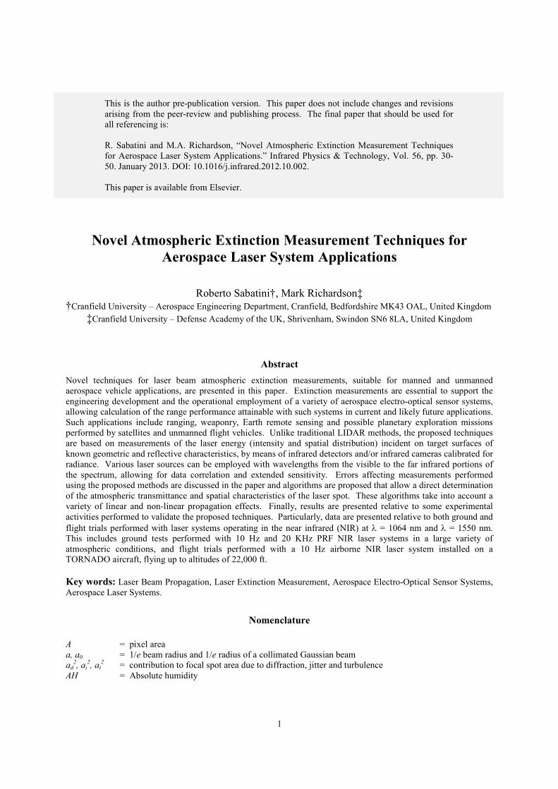
suitable for a variety of platform applications including aircraft, satellites, Unmanned Flight Vehicles (UFV),
parachute/gliding vehicles, Roving Surface Vehicles (RSV), or Permanent Surface Installations (PSI). They are
based on direct measurement of the laser energy incident on target surfaces of known geometric and reflective
characteristics, such as Spectral Reflectance (ρ) and Bidirectional Reflectance Distribution Function (BRDF). A
depiction of the possible platform applications is presented in Fig. 1. For vertical/oblique path measurements, the
laser source can be located on Satellites, Gliders or UFVs flying in the planet atmosphere at different altitudes (but
also manned aircrafts on Earth or their future equivalents on other planets), while for surface layer measurements the
laser source could be mounted on RSV or even on PSI turrets at different fixed locations on the planet surface.
Surface Target
Surface Lasers
Outer Satellite Target
Outer Satellite Laser
Glider/Balloon or
Inner Satellite
Target
Aircraft, UAV or Inner
Satellite Laser
Glider/Balloon Laser
Atmosphere
1
3
4
2
5
6
87
9
Figure 1. Possible platform applications.
2. Laser Beam Propagation Overview
Several research activities have been undertaken for characterizing and modelling linear and non-linear atmospheric
propagation effects on laser beams. In this paper, we focus on phenomena affecting the peak irradiance at a distant
location from the laser output aperture.
4
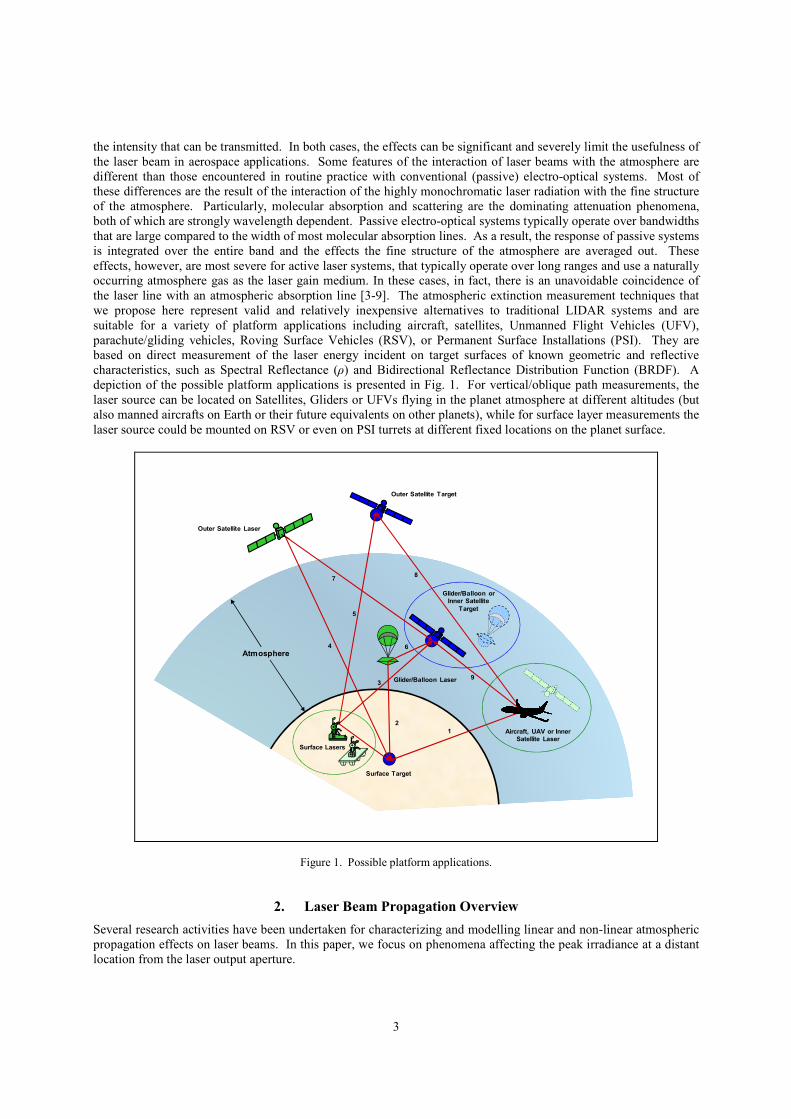
2.1 Atmospheric Transmittance
Attenuation of laser radiation in the atmosphere is described by Beer's law [1]:
( ) z
atm eI
zI γτ −==0
(1)
where τatm is the transmittance, γ is the attenuation coefficient (extinction), and z is the length of the transmission
path. Since the attenuation coefficient is a function of the molecular and aerosol particle concentrations along the
path, Eq. (1) becomes:
( )∫=
−z
dzz
atm e 0γ
τ (2)
were the attenuation coefficient is determined by four individual processes: molecular absorption, molecular
scattering, aerosol absorption, and aerosol scattering. Therefore:
aamm βαβαγ +++= (3)
where α is the absorption coefficient, β is the scattering coefficient, and the subscripts m and a designate the
molecular and aerosol processes, respectively. Each coefficient in Eq. (3) depends on the wavelength of the laser
radiation. We find it convenient at times to discuss absorption and scattering in terms of the absorption and
scattering cross sections (σa and σs, respectively) of the individual particles that are involved. Therefore:
aa Nσα = (4)
and
ssNσβ = (5)
where Na and Ns are the concentrations of the absorbing and scattering species respectively. In the absence of
precipitation, the Earth’s atmosphere contains finely dispersed solid and liquid particles (of ice, dust, aromatic and
organic material) that vary in size from a cluster of a few molecules to particles of about 20 µm in radius. Particles
larger than this remain airborne for a short time and are only found close to their sources. Such a colloidal system,
in which a gas (in this case, air) is the continuous medium and particles of solid or liquid are dispersed, is known as
an aerosol. Aerosol attenuation coefficients depend considerably on the dimensions, chemical composition, and
ncentration of aerosol particles. These particles are generally assumed to be homogeneous spheres that are
characterized by two parameters: the radius and the index of refraction. In general, the index of refraction is
complex. Therefore, we can write:
( )κinn
kiniknn −=
−=−= 11~ (6)
where n and k are the real and imaginary parts and κ = k/n is known as the extinction coefficient. In general, both n
and k are functions of the frequency of the incident radiation. The imaginary part (which arises from a finite
conductivity of the particle) is a measure of the absorption. In fact, k is referred to as the absorption constant. It is
related to the absorption coefficient α of Eqs. (3) and (4) by:
c
fkπα
4= (7)
where c is the speed of light in a vacuum and f is the frequency of the incident radiation. The scattering coefficient
β in Eqs. (3) and (5) also depends on the frequency of the incident radiation as well as the index of refraction and
radius of the scattering particle. The incident electromagnetic wave, which is assumed to be a plane wave in a given
polarization state, produces forced oscillations of the bound and free charges within the sphere. These oscillating
charges in turn produce secondary fields internal and external to the sphere. The resulting field at any point is the
vector sum of the primary (plane wave) and secondary fields. Once the resultant field has been determined, the
scattering cross section (σs) is obtained from the following relationship:
5
T
ss
M
P=σ (8)
where Ps is the total power scattered by scatterer, and |M|T is the time-averaged incident Poynting vector. In the
scattering process there is no loss of energy but only a directional redistribution which may lead to a significant
reduction in beam intensity for large path lengths. As is indicated in Table 1, the physical size of the scatterer
determines the type of scattering process. Thus, air molecules which are typically several angstrom units in
diameter lead to Rayleigh scattering, whereas the aerosols scatter light in accordance with the Mie theory.
Furthermore, when the scatterers are relatively large, such as the water droplets found in fog, clouds, rain, or snow,
the scattering process is more properly described by diffraction theory.
Table 1. Types of atmospheric scattering.
Type of Scattering Size of Scatterer
Rayleigh Scattering Larger than electron but smaller than λ
Mie Scattering Comparable in size to λ
Non-selective Scattering Much larger than λ
The atmospheric composition of Earth is largely governed by the by-products of the life that it sustains. Earth's
atmosphere consists principally of a roughly 78:20 ratio of nitrogen (N2) and oxygen (O2), plus substantial water
vapour, with a minor proportion of carbon dioxide (CO2). Due to human activities, the CO2 concentrations are
constantly growing (this has been recognized as a main contributing factor to climate change and global warming).
There are also smaller concentrations of hydrogen, and of helium, argon, and other noble gases. Volatile pollutants,
including various types of man-made gases and aerosols with largely variable particle size distributions are also
present. For the wavelength range of greater interest in laser beam propagation (the visible region to about 15 µm)
the principal atmospheric absorbers are the molecules of water, CO2 and ozone. Attenuation occurs because these
molecules selectively absorb radiation by changing vibration and rotation energy states. The two gases present in
greatest abundance in the Earth's atmosphere, nitrogen and oxygen, are homonuclear, which means that they possess
no electric dipole moment and therefore do not exhibit molecular absorption bands. The Earth’s atmospheric
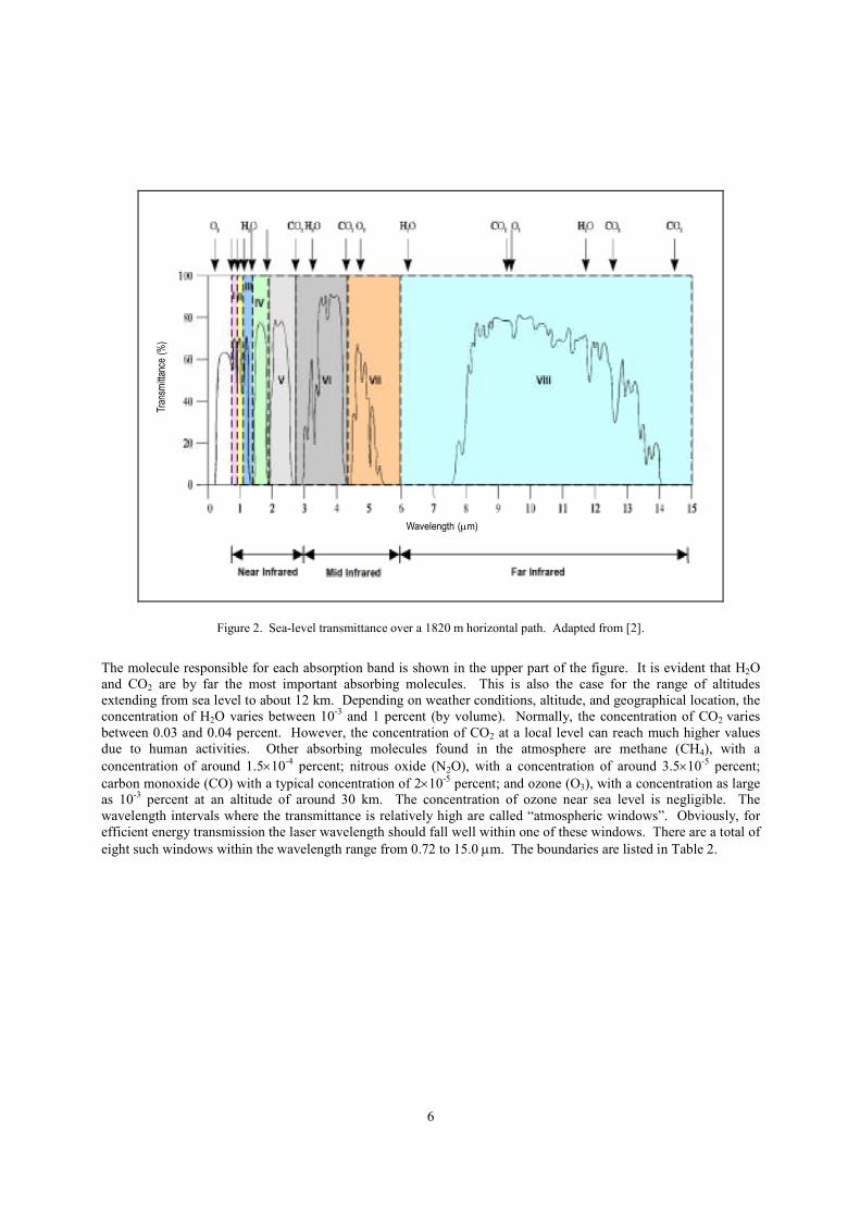
spectral transmittance τ(%) measured over a 1820-m horizontal path at sea-level is shown in Fig. 2.
6
Tran
smitt
ance
(%
)
Wavelength (µm)
Figure 2. Sea-level transmittance over a 1820 m horizontal path. Adapted from [2].
The molecule responsible for each absorption band is shown in the upper part of the figure. It is evident that H2O
and CO2 are by far the most important absorbing molecules. This is also the case for the range of altitudes
extending from sea level to about 12 km. Depending on weather conditions, altitude, and geographical location, the
concentration of H2O varies between 10-3
and 1 percent (by volume). Normally, the concentration of CO2 varies
between 0.03 and 0.04 percent. However, the concentration of CO2 at a local level can reach much higher values
due to human activities. Other absorbing molecules found in the atmosphere are methane (CH4), with a
concentration of around 1.5×10⁻⁴
percent; nitrous oxide (N2O), with a concentration of around 3.5×10⁻⁵
percent;
carbon monoxide (CO) with a typical concentration of 2×10⁻⁵
percent; and ozone (O3), with a concentration as large
as 10-3
percent at an altitude of around 30 km. The concentration of ozone near sea level is negligible. The
wavelength intervals where the transmittance is relatively high are called “atmospheric windows”. Obviously, for
efficient energy transmission the laser wavelength should fall well within one of these windows. There are a total of
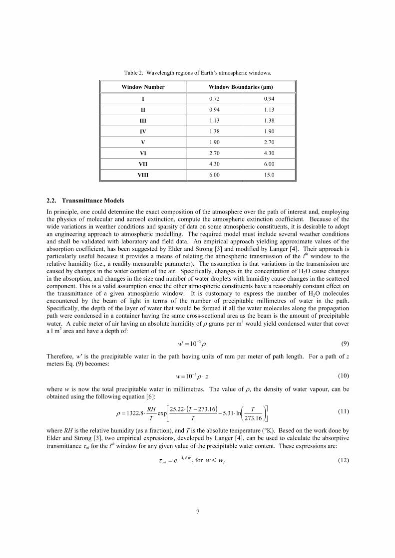
eight such windows within the wavelength range from 0.72 to 15.0 µm. The boundaries are listed in Table 2.
7
Table 2. Wavelength regions of Earth’s atmospheric windows.
Window Number Window Boundaries (µm)
I 0.72 0.94
II 0.94 1.13
III 1.13 1.38
IV 1.38 1.90
V 1.90 2.70
VI 2.70 4.30
VII 4.30 6.00
VIII 6.00 15.0
2.2. Transmittance Models
In principle, one could determine the exact composition of the atmosphere over the path of interest and, employing
the physics of molecular and aerosol extinction, compute the atmospheric extinction coefficient. Because of the
wide variations in weather conditions and sparsity of data on some atmospheric constituents, it is desirable to adopt
an engineering approach to atmospheric modelling. The required model must include several weather conditions
and shall be validated with laboratory and field data. An empirical approach yielding approximate values of the
absorption coefficient, has been suggested by Elder and Strong [3] and modified by Langer [4]. Their approach is
particularly useful because it provides a means of relating the atmospheric transmission of the ith
window to the
relative humidity (i.e., a readily measurable parameter). The assumption is that variations in the transmission are
caused by changes in the water content of the air. Specifically, changes in the concentration of H2O cause changes
in the absorption, and changes in the size and number of water droplets with humidity cause changes in the scattered
component. This is a valid assumption since the other atmospheric constituents have a reasonably constant effect on
the transmittance of a given atmospheric window. It is customary to express the number of H2O molecules
encountered by the beam of light in terms of the number of precipitable millimetres of water in the path.
Specifically, the depth of the layer of water that would be formed if all the water molecules along the propagation
path were condensed in a container having the same cross-sectional area as the beam is the amount of precipitable
water. A cubic meter of air having an absolute humidity of ρ grams per m3 would yield condensed water that cover
a l m2 area and have a depth of:
ρ310−=′w (9)
Therefore, w' is the precipitable water in the path having units of mm per meter of path length. For a path of z
meters Eq. (9) becomes:
zw ⋅= − ρ310 (10)
where w is now the total precipitable water in millimetres. The value of ρ, the density of water vapour, can be
obtained using the following equation [6]:
( )
⋅−−⋅
⋅=16.273
ln31.516.27322.25
exp8.1322T
T
T
T
RHρ (11)
where RH is the relative humidity (as a fraction), and T is the absolute temperature (°K). Based on the work done by
Elder and Strong [3], two empirical expressions, developed by Langer [4], can be used to calculate the absorptive
transmittance τai for the ith
window for any given value of the precipitable water content. These expressions are:
wA
aiie
−=τ , for iww < (12)
8
i
w
wk i
iai
β
τ
= , for iww > (13)
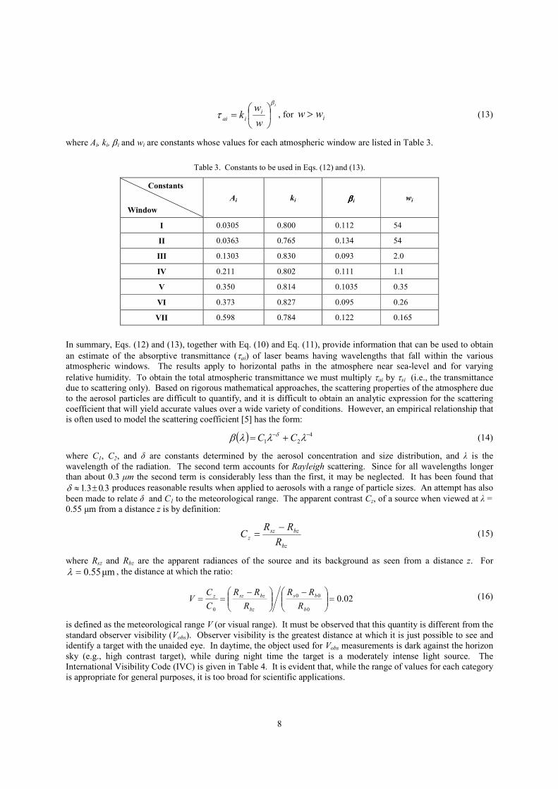
where Ai, ki, βi and wi are constants whose values for each atmospheric window are listed in Table 3.
Table 3. Constants to be used in Eqs. (12) and (13).
Constants
Window
Ai
ki
ββββi
wi
I 0.0305 0.800 0.112 54
II 0.0363 0.765 0.134 54
III 0.1303 0.830 0.093 2.0
IV 0.211 0.802 0.111 1.1
V 0.350 0.814 0.1035 0.35
VI 0.373 0.827 0.095 0.26
VII 0.598 0.784 0.122 0.165
In summary, Eqs. (12) and (13), together with Eq. (10) and Eq. (11), provide information that can be used to obtain
an estimate of the absorptive transmittance (τai) of laser beams having wavelengths that fall within the various
atmospheric windows. The results apply to horizontal paths in the atmosphere near sea-level and for varying
relative humidity. To obtain the total atmospheric transmittance we must multiply τai by τsi (i.e., the transmittance
due to scattering only). Based on rigorous mathematical approaches, the scattering properties of the atmosphere due
to the aerosol particles are difficult to quantify, and it is difficult to obtain an analytic expression for the scattering
coefficient that will yield accurate values over a wide variety of conditions. However, an empirical relationship that
is often used to model the scattering coefficient [5] has the form:
( ) 4
21
−− += λλλβ δ CC (14)
where C1, C2, and δ are constants determined by the aerosol concentration and size distribution, and λ is the
wavelength of the radiation. The second term accounts for Rayleigh scattering. Since for all wavelengths longer
than about 0.3 µm the second term is considerably less than the first, it may be neglected. It has been found that
3031 .. ±≈δ produces reasonable results when applied to aerosols with a range of particle sizes. An attempt has also
been made to relate δ and C1 to the meteorological range. The apparent contrast Cz, of a source when viewed at λ =
0.55 µm from a distance z is by definition:
bz
bzsz
zR
RRC
−= (15)
where Rsz and Rbz are the apparent radiances of the source and its background as seen from a distance z. For
µm 55.0=λ , the distance at which the ratio:
02.00
00
0
=
−
−==
b
bs
bz
bzszz
R
RR
R
RR
C
CV (16)
is defined as the meteorological range V (or visual range). It must be observed that this quantity is different from the
standard observer visibility (Vobs). Observer visibility is the greatest distance at which it is just possible to see and
identify a target with the unaided eye. In daytime, the object used for Vobs measurements is dark against the horizon
sky (e.g., high contrast target), while during night time the target is a moderately intense light source. The
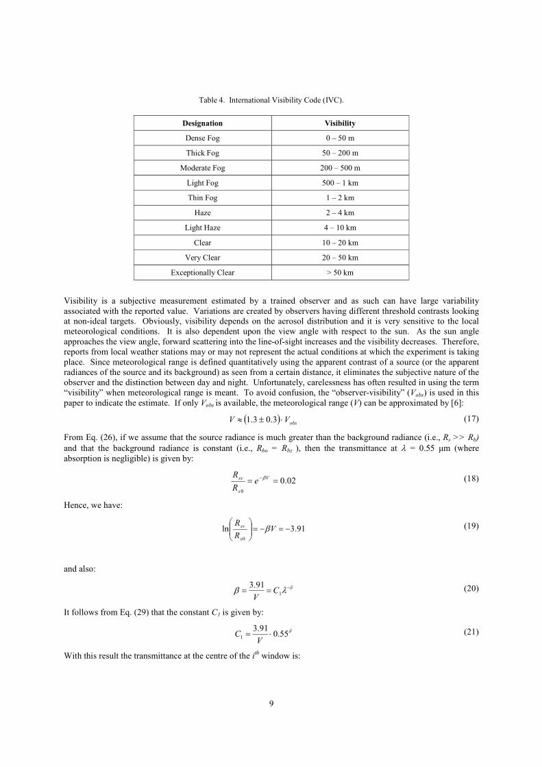
International Visibility Code (IVC) is given in Table 4. It is evident that, while the range of values for each category
is appropriate for general purposes, it is too broad for scientific applications.
9
Table 4. International Visibility Code (IVC).
Designation Visibility
Dense Fog 0 – 50 m
Thick Fog 50 – 200 m
Moderate Fog 200 – 500 m
Light Fog 500 – 1 km
Thin Fog 1 – 2 km
Haze 2 – 4 km
Light Haze 4 – 10 km
Clear 10 – 20 km
Very Clear 20 – 50 km
Exceptionally Clear > 50 km
Visibility is a subjective measurement estimated by a trained observer and as such can have large variability
associated with the reported value. Variations are created by observers having different threshold contrasts looking
at non-ideal targets. Obviously, visibility depends on the aerosol distribution and it is very sensitive to the local
meteorological conditions. It is also dependent upon the view angle with respect to the sun. As the sun angle
approaches the view angle, forward scattering into the line-of-sight increases and the visibility decreases. Therefore,
reports from local weather stations may or may not represent the actual conditions at which the experiment is taking
place. Since meteorological range is defined quantitatively using the apparent contrast of a source (or the apparent
radiances of the source and its background) as seen from a certain distance, it eliminates the subjective nature of the
observer and the distinction between day and night. Unfortunately, carelessness has often resulted in using the term
“visibility” when meteorological range is meant. To avoid confusion, the “observer-visibility” (Vobs) is used in this
paper to indicate the estimate. If only Vobs is available, the meteorological range (V) can be approximated by [6]:
( ) obsVV ⋅±≈ 3.03.1 (17)
From Eq. (26), if we assume that the source radiance is much greater than the background radiance (i.e., Rs >> Rb)
and that the background radiance is constant (i.e., Rbo = Rbz ), then the transmittance at λ = 0.55 µm (where
absorption is negligible) is given by:
02.00
== − V
s
sv eR
R β (18)
Hence, we have:
91.3ln0
−=−=
V
R
R
s
sv β (19)
and also:
δλβ −== 1
91.3C
V (20)
It follows from Eq. (29) that the constant C1 is given by:
δ55.091.3
1 ⋅=V
C (21)
With this result the transmittance at the centre of the ith
window is:
10
z
V
si
i
e⋅
⋅−
−
=
δλ
τ 55.0
91.3
(22)
where λi must be expressed in microns. If, because of haze, the meteorological range is less than 6 km, the exponent
δ is related to the meteorological range by the following empirical formula:
3585.0 V=δ (23)
where V is in kilometres. When V ≥ 6 km, the exponent δ can be calculated by:
025.10057.0 +⋅= Vδ (24)
For exceptionally good visibility δ = 1.6, and for average visibility δ ≈ 1.3. In summary, Eq. (32), together with the
appropriate value for δ, allows to compute the scattering transmittance at the centre of the ith window for any
propagation path, if the meteorological range V is known. It is important to note here that in general the
transmittance will, of course, also be affected by atmospheric absorption, which depending on the relative humidity
and temperature may be larger than τsi.
2.3. Propagation Through Haze and Precipitation
Haze refers to the small particles suspended in the air. These particles consist of microscopic salt crystals, very fine
dust, and combustion products. Their radii are less than 0.5 µm. During periods of high humidity, water molecules
condense onto these particles, which then increase in size. It is essential that these condensation nuclei be available
before condensation can take place. Since salt is quite hygroscopic, it is by far the most important condensation
nucleus. Fog occurs when the condensation nuclei grow into water droplets or ice crystals with radii exceeding 0.5
µm. Clouds are formed in the same way; the only distinction between fog and clouds is that one touches the ground
while the other does not. By convention fog limits the visibility to less than 1 km, whereas in a mist the visibility is
greater than 1 km. We know that in the early stages of droplet growth the Mie attenuation factor K depends strongly
on the wavelength. When the drop has reached a radius a ≈ 10 λ the value of K approaches 2, and the scattering is
now independent of wavelength, i.e., it is non-selective. Since most of the fog droplets have radii ranging from 5 to
15 µm they are comparable in size to the wavelength of infrared radiation. Consequently the value of the scattering
cross section is near its maximum. It follows that the transmission of fogs in either the visible or IR spectral region is
poor for any reasonable path length. This of course also applies to clouds. Since haze particles are usually less than
0.5 µm, we note that for laser beams in the IR spectral region 1<<λa and the scattering is not an important
attenuation mechanism. This explains why photographs of distant objects are sometimes made with infrared-
sensitive film that responds to wavelengths out to about 0.85 µm. At this wavelength the transmittance of a light
haze is about twice that at 0.5 µm. Raindrops are of course many times larger than the wavelengths of laser beams.
As a result there is no wavelength-dependent scattering. The scattering coefficient does, however, depend strongly
on the size of the drop. Middleton [5, 6] has shown that the scattering coefficient with rain is given by:
3
61025.1a
txrain
∆∆⋅= −β (25)
where ∆x/∆t is the rainfall rate in centimetres of depth per second and a is the radius of the drops in centimetres.
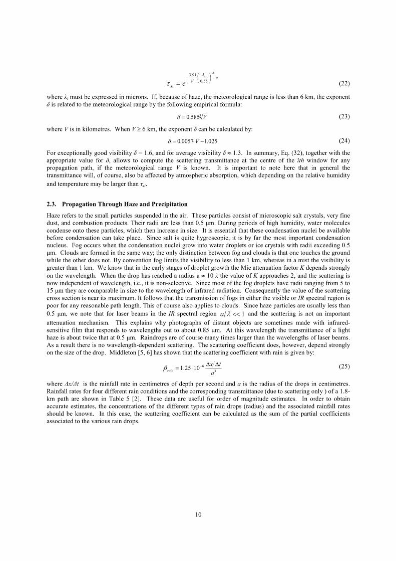
Rainfall rates for four different rain conditions and the corresponding transmittance (due to scattering only ) of a 1.8-
km path are shown in Table 5 [2]. These data are useful for order of magnitude estimates. In order to obtain
accurate estimates, the concentrations of the different types of rain drops (radius) and the associated rainfall rates
should be known. In this case, the scattering coefficient can be calculated as the sum of the partial coefficients
associated to the various rain drops.
11
Table 5. Transmittance of a 1.8-km path through rain.
Rainfall (cm/h) Transmittance (1.8 km path)
0.25 0.88
1.25 0.74
2.5 0.65
10.0 0.38
A simpler approach, used in LOWTRAN, gives good approximations of the results obtained with Eq. (25) for most
concentrations of different rain particles. Particularly, the scattering coefficient with rain has been empirically
related only to the rainfall rate tx ∆∆ (expressed in mm/hour), as follows [7]:
63.0
365.0
∆∆
⋅≈t
xrainβ (26)
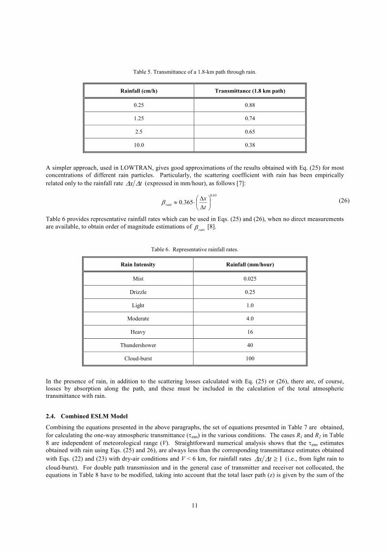
Table 6 provides representative rainfall rates which can be used in Eqs. (25) and (26), when no direct measurements
are available, to obtain order of magnitude estimations of rainβ [8].
Table 6. Representative rainfall rates.
Rain Intensity Rainfall (mm/hour)
Mist 0.025
Drizzle 0.25
Light 1.0
Moderate 4.0
Heavy 16
Thundershower 40
Cloud-burst 100
In the presence of rain, in addition to the scattering losses calculated with Eq. (25) or (26), there are, of course,
losses by absorption along the path, and these must be included in the calculation of the total atmospheric
transmittance with rain.
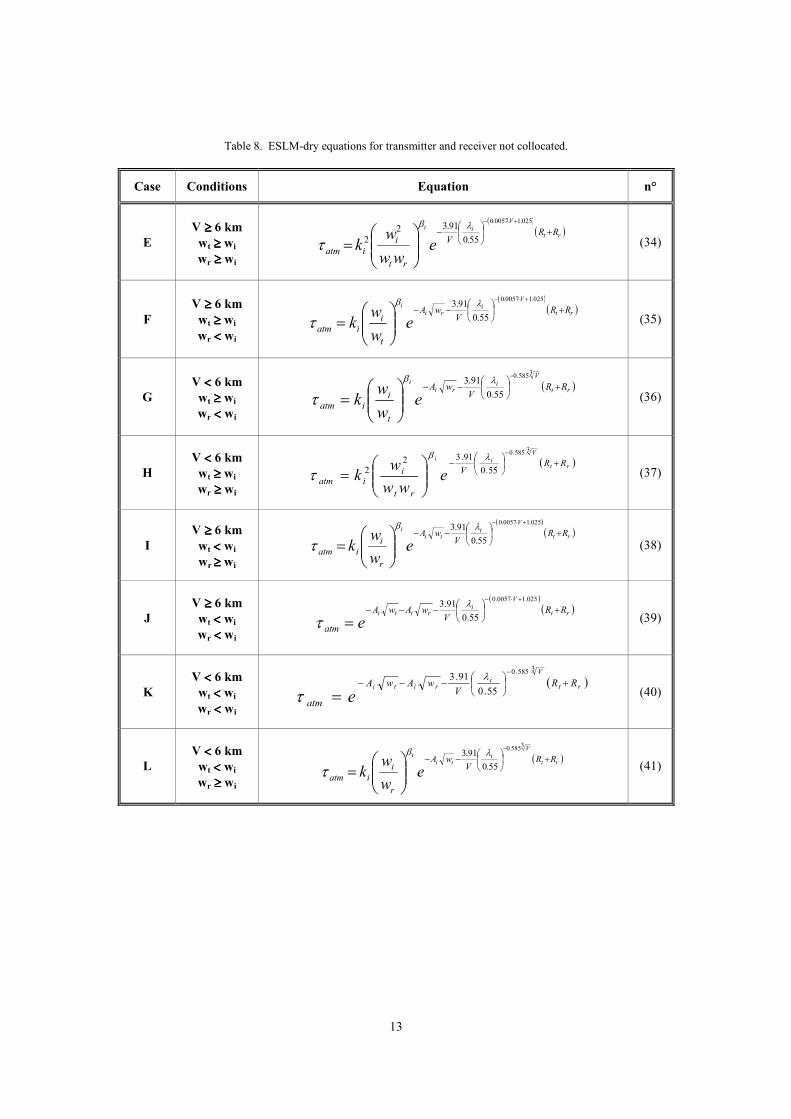
2.4. Combined ESLM Model
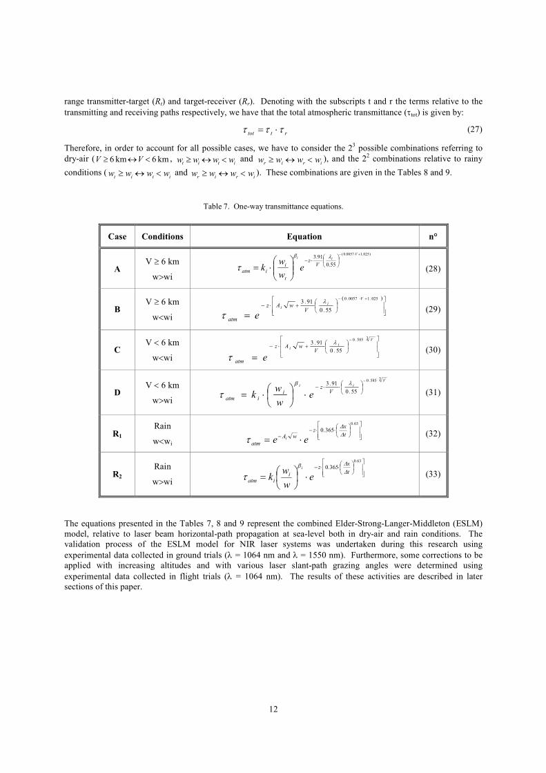
Combining the equations presented in the above paragraphs, the set of equations presented in Table 7 are obtained,
for calculating the one-way atmospheric transmittance (τatm) in the various conditions. The cases R1 and R2 in Table
8 are independent of meteorological range (V). Straightforward numerical analysis shows that the τatm estimates
obtained with rain using Eqs. (25) and 26), are always less than the corresponding transmittance estimates obtained
with Eqs. (22) and (23) with dry-air conditions and V < 6 km, for rainfall rates 1≥tx ∆∆ (i.e., from light rain to
cloud-burst). For double path transmission and in the general case of transmitter and receiver not collocated, the
equations in Table 8 have to be modified, taking into account that the total laser path (z) is given by the sum of the
12
)025.10057.0(
55.0
91.3+⋅−
⋅⋅−
⋅=
Vii
Vz
t
iiatm e
w
wk
λβ
τ
range transmitter-target (Rt) and target-receiver (Rr). Denoting with the subscripts t and r the terms relative to the
transmitting and receiving paths respectively, we have that the total atmospheric transmittance (τtot) is given by:
rttot τττ ⋅= (27)
Therefore, in order to account for all possible cases, we have to consider the 23 possible combinations referring to
dry-air ( km 6km 6 <↔≥ VV , itit wwww <↔≥ and
irir wwww <↔≥ ), and the 22 combinations relative to rainy
conditions (itit wwww <↔≥ and
irir wwww <↔≥ ). These combinations are given in the Tables 8 and 9.
Table 7. One-way transmittance equations.
Case Conditions Equation n°
A V ≥ 6 km
w>wi
(28)
B V ≥ 6 km
w<wi
( )
+⋅−+⋅−
=
025100570
550
913.V.
ii
.V
.wAz
atm e
λ
τ
(29)
C V < 6 km
w<wi
+⋅−
−
=
35850
550
913V.
ii
.V
.wAz
atm e
λ
τ
(30)
D V < 6 km
w>wi
35850
550
913V.
ii
.V
.z
iiatm e
w
wk
−
⋅⋅−
⋅
⋅=λβ
τ
(31)
R1 Rain
w<wi
⋅⋅−− ⋅=
630
3650
.
it
x.z
wA
atm ee∆∆
τ
(32)
R2 Rain
w>wi
⋅⋅−
⋅
=
630
3650
.
it
x.z
iiatm e
w
wk
∆∆β
τ
(33)
The equations presented in the Tables 7, 8 and 9 represent the combined Elder-Strong-Langer-Middleton (ESLM)
model, relative to laser beam horizontal-path propagation at sea-level both in dry-air and rain conditions. The
validation process of the ESLM model for NIR laser systems was undertaken during this research using
experimental data collected in ground trials (λ = 1064 nm and λ = 1550 nm). Furthermore, some corrections to be
applied with increasing altitudes and with various laser slant-path grazing angles were determined using
experimental data collected in flight trials (λ = 1064 nm). The results of these activities are described in later
sections of this paper.
13
Table 8. ESLM-dry equations for transmitter and receiver not collocated.
Case Conditions Equation n°
E
V ≥≥≥≥ 6 km
wt ≥≥≥≥ wi
wr ≥≥≥≥ wi
(34)
F
V ≥≥≥≥ 6 km
wt ≥≥≥≥ wi
wr <<<< wi
(35)
G
V <<<< 6 km
wt ≥≥≥≥ wi
wr <<<< wi
(36)
H
V <<<< 6 km
wt ≥≥≥≥ wi
wr ≥≥≥≥ wi
(37)
I
V ≥≥≥≥ 6 km
wt <<<< wi
wr ≥≥≥≥ wi
(38)
J
V ≥≥≥≥ 6 km
wt <<<< wi
wr <<<< wi
(39)
K
V <<<< 6 km
wt <<<< wi
wr <<<< wi
(40)
L
V <<<< 6 km
wt <<<< wi
wr ≥≥≥≥ wi
(41)
( )( )rt
V
iiRR
V
rt
i
iatm eww
wk
+
−
+⋅−
=
025.10057.0
55.0
91.32
2
λβ
τ
( )( )rt
Vi
rii
RRV
wA
t
i
iatm ew
wk
+
−−
+⋅−
=
025.10057.0
55.0
91.3 λβ
τ
( )rt
Vi
ri
iRR
VwA
t
iiatm e
w
wk
+
−−
−
=
3585.0
55.0
91.3 λβ
τ
( )rt
V
iiRR
V
rt
iiatm e
ww
wk
+
−
−
=
3585.0
55.0
91.322
λβ
τ
( )( )rt
V
iti
iRR
VwA
r
i
iatm ew
wk
+
−−
+⋅−
=
025.10057.0
55.0
91.3 λβ
τ
( )( )rt
V
iriti RR
VwAwA
atm e+
−−−
+⋅−
=
025.10057.0
55.0
91.3 λ
τ
( )rt
V
iriti RR
VwAwA
atm e+
−−−−
=
3585.0
55.0
91.3 λ
τ
( )rt
V
iti
iRR
VwA
r
i
iatm ew
wk
+
−−
−
=
3585.0
55.0
91.3 λβ
τ
14
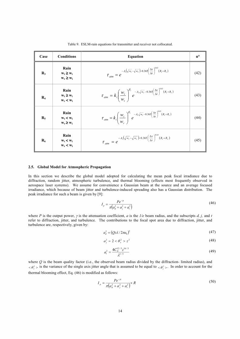
Table 9. ESLM-rain equations for transmitter and receiver not collocated.
Case Conditions Equation n°
R3
Rain
wt ≥≥≥≥ wi
wr ≥≥≥≥ wi
(42)
R4
Rain
wt ≥≥≥≥ wi
wr <<<< wi
(43)
R5
Rain
wt <<<< wi
wr ≥≥≥≥ wi
(44)
R6
Rain
wt <<<< wi
wr <<<< wi
(45)
2.5. Global Model for Atmospheric Propagation
In this section we describe the global model adopted for calculating the mean peak focal irradiance due to
diffraction, random jitter, atmospheric turbulence, and thermal blooming (effects most frequently observed in
aerospace laser systems). We assume for convenience a Gaussian beam at the source and an average focused
irradiance, which because of beam jitter and turbulence-induced spreading also has a Gaussian distribution. The
peak irradiance for such a beam is given by [9]:
( )222
tjd
z
paaa
PeI
++=
−
π
γ (46)
where P is the output power, γ is the attenuation coefficient, a is the 1/e beam radius, and the subscripts d, j, and t
refer to diffraction, jitter, and turbulence. The contributions to the focal spot area due to diffraction, jitter, and
turbulence are, respectively, given by:
( )20
2 2/ aQzad πλ= (47)
2222 za xj ><= θ (48)
5/2
5/165/122 4
λzC
a Nt = (49)
where Q is the beam quality factor (i.e., the observed beam radius divided by the diffraction- limited radius), and
>< 2
xθ is the variance of the single axis jitter angle that is assumed to be equal to >< 2
yθ . In order to account for the
thermal blooming effect, Eq. (46) is modified as follows:
( ) R
aaa
PeI
tjd
z
p ×++
=−
222π
γ (50)
( ) ( )rtrti RRt
xwwA
atm e+
∆
∆−−−
=
63.0
365.0
τ
( )rtri
iRR
t
xwA
t
i
iatm ew
wk
+
∆
∆−−
=
63.0
365.0β
τ
( )rtti
iRR
t
xwA
r
i
iatm ew
wk
+
∆
∆−−
=
63.0
365.0β
τ
( ) ( )rtrti RRt
xwwA
atm e+
∆
∆−−−
=
63.0
365.0
τ
15
where R is the ratio of the bloomed IB to unbloomed IUB peak irradiance. An empirical relationship for R found for
propagation in the Earth’s atmosphere is the following:
20625.01
1
NI
IR
UB
B
+== (51)
where N, the thermal distortion parameter, is a dimensionless quantity that indicates the degree or strength of
thermal distortion. Here N is given by:
−= ∫∫ ''
)''()''(
)''exp('
)'(
2'
0
2
0
2
0
0
0
20 dzzvza
zvadz
za
a
zNN
zz γ (52)
where
3
000
2
0acvd
PznN
p
mT
πα−
= (53)
is the distortion parameter for a collimated Gaussian beam of 1/e radius a0 and uniform wind velocity v0 in the weak
attenuation limit (γz << 1). The quantities nT , d0 , and cp are, respectively, the coefficients of index change with
respect to temperature, density, and specific heat at constant pressure, and P and z are the laser output power and
range, respectively. Eq. (50) is the propagation equation for Gaussian beams. It can be used to calculate the
propagation performance of different laser wavelengths. Considering both propagation performances and output
power characteristics of state-of-the-art systems, good candidate lasers covering the entire infrared spectrum are
listed below:
- CO2 → λ = 10.591 µm
- CO → λ = 4.9890 µm
- DF → λ = 3.8007 µm
- HF → λ = 2.9573 µm
- Er:Fiber → λ = 1.5500 µm
- Nd:YAG → λ = 1.0640 µm
- Ar → λ = 0.5145 µm
- N2 → λ = 0.3371 µm
In general, for the mid to far-IR lasers (e.g., CO2, CO and DF) the peak irradiance increases with decreasing
wavelength in clear and moderate turbulence conditions. For the near to mid-IR lasers (eg., HF, Ar, and Nd:YAG
lasers), the peak irradiance is reduced significantly by aerosol scattering and turbulence. It is interesting to note that
for the CO2 wavelength, which is dominated by thermal blooming due to stronger molecular absorption, the peak
irradiance is relatively insensitive to both turbulence and aerosol effects. At the shorter wavelengths the effects of
turbulence and aerosol attenuation produce wide variations in the peak irradiance. The importance of both aerosol
scattering and turbulence effects clearly increases at the shorter wavelengths (eg., Ar, N2, Er:Fiber and Nd:YAG
lasers). In most cases, the near to mid-IR regions offer the best overall transmission characteristics; in particular, the
3.8-µm DF wavelength is optimum for varying aerosol and turbulence conditions. In summary, the propagation of
high-power laser beams through the atmosphere is affected by a host of optical phenomena. For CW beams the
most significant phenomena are absorption and scattering by molecules and aerosols, as well as atmospheric
turbulence and thermal blooming. In general, thermal blooming tends to dominate the longer wavelengths (5-10
µm), while aerosol and turbulence effects are more important at the shorter wavelengths and result in larger
variations in peak irradiance in the focal plane as atmospheric conditions change. Some of these effects can be
overcome by using laser pulses rather than CW beams and/or adaptive optical techniques.
3. Extinction Measurement Techniques
We propose various methods for accurate Laser Extinction Measurement (LEM) that use combinations of different
pulsed laser sources, passive infrared imaging systems and direct detection electro-optics systems. The proposed
methods are suitable for both Earth remote sensing missions and likely future planetary exploration missions
performed by using Satellites, Unmanned Flight Vehicles (UFV), Gliders/Parachutes/Balloons (GPB), Roving
Surface Vehicles (RSV), or Permanent Surface Installations (PSI). For vertical/oblique paths sounding, the laser
16
source can be located on Satellites (GEO, MEO and LEO) or UFV flying in the planet atmosphere at different
altitudes (but also manned aircrafts on Earth or their future equivalents on other planets), while for surface layer
measurements the laser source could be mounted on RSV or even on PSI turrets at different fixed locations on the
planet surface. All proposed methods offer relative advantages and limitations in different scenarios.
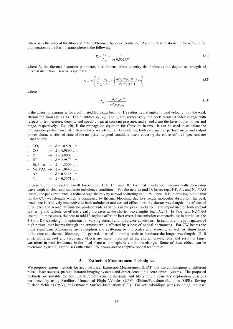
3.2 LEM-1 Method
The first method for atmospheric extinction measurements (LEM-1) is depicted in Fig. 3. In this case, the pulse
laser energy (transmitted from an aircraft, satellite, UFV, etc.) incident on a reference target surface of known
geometric and reflective characteristics (ρ, BRDF, inclination, etc.), is measured by using NIR cameras with
associated image processing software and incorporating appropriate algorithms to perform radiance measurements
in the focal plane. Based on the LEM-1 method, two Energy Measurement Techniques (EMT) were developed for
non-calibrated (EMT-1) and calibrated (EMT-2) NIR cameras. For the case of non-calibrated IR cameras (EMT-1),
the reference target has to be instrumented with suitable IR detectors (e.g., Pyroelectric Probes – PEPs) with
associated optics.
0
15
30
0
2000
4000
6000
8000
10000
12000
14000
16000
0 5
10
15
20
25
30
35
40
Gray Scale Intensity
Pixels
GLTD Spot PIM- 4000 m -
Camera Frame (Target)
0
70
140
210
280
350
420
490
560
- 4000 m -
0
70
140
210
280
350
420
490
560
E( λλλλ ) = 52.76 mJ
GLTD Spot Energy Profile
Energy
Pixels
Analysis Sub-frame
Figure 3. LTM-B Method.
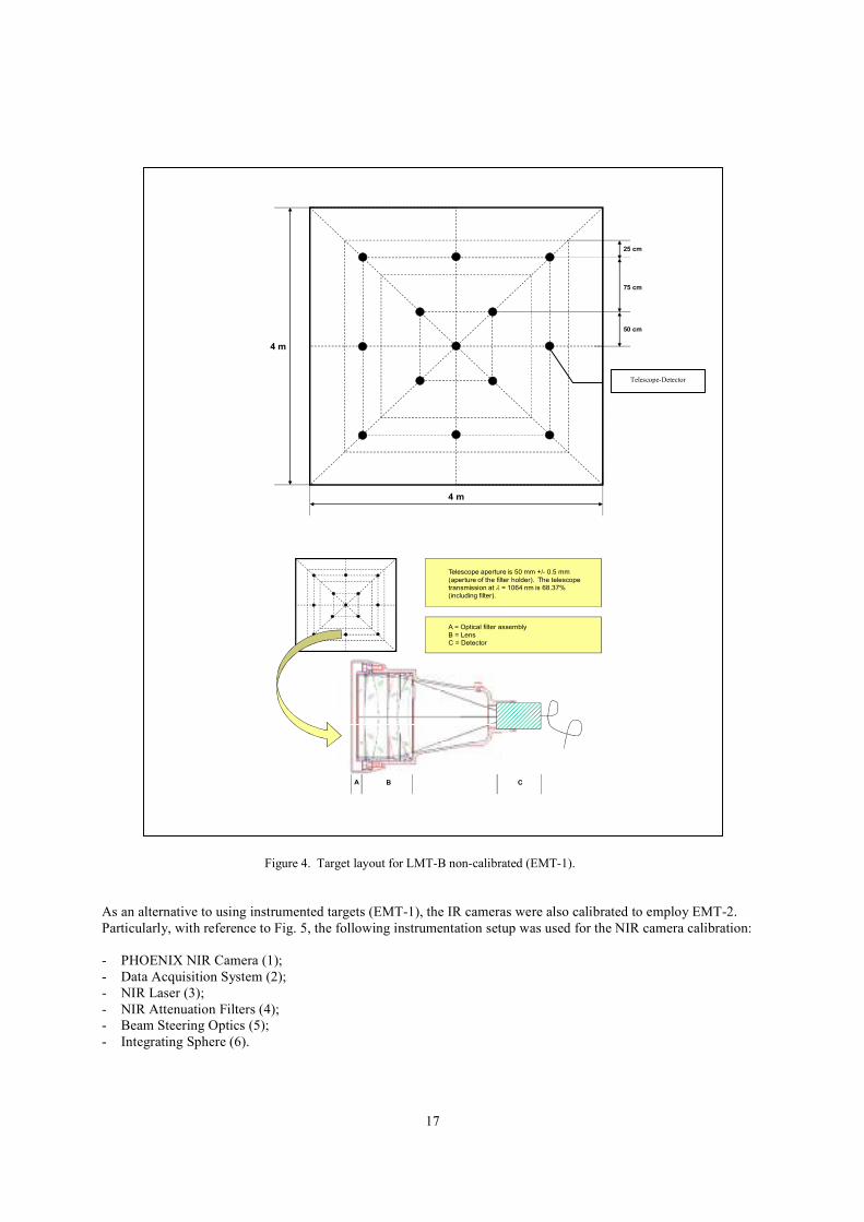
The layout of the instrumented target used for the LEM-1 ground and flight trials is shown in Fig. 4.
17
4 m
4 m
50 cm
75 cm
25 cm
.
.
.
. .
.
.
.
Telescope aperture is 50 mm +/- 0.5 mm
(aperture of the filter holder). The telescope
transmission at λ = 1064 nm is 68.37%
(including filter).
A B C
A = Optical filter assembly
B = Lens
C = Detector
Figure 4. Target layout for LMT-B non-calibrated (EMT-1).
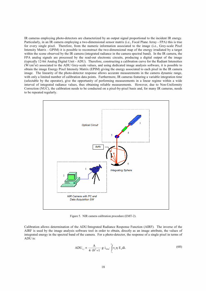
As an alternative to using instrumented targets (EMT-1), the IR cameras were also calibrated to employ EMT-2.
Particularly, with reference to Fig. 5, the following instrumentation setup was used for the NIR camera calibration:
- PHOENIX NIR Camera (1);
- Data Acquisition System (2);
- NIR Laser (3);
- NIR Attenuation Filters (4);
- Beam Steering Optics (5);
- Integrating Sphere (6).
Telescope-Detector
18
IR cameras employing photo-detectors are characterized by an output signal proportional to the incident IR energy.
Particularly, in an IR camera employing a two-dimensional sensor matrix (i.e., Focal Plane Array - FPA) this is true
for every single pixel. Therefore, from the numeric information associated to the image (i.e., Grey-scale Pixel
Intensity Matrix - GPIM) it is possible to reconstruct the two-dimensional map of the energy irradiated by a target
within the scene observed by the IR camera (integrated radiance in the camera spectral band). In the IR camera, the
FPA analog signals are processed by the read-out electronic circuits, producing a digital output of the image
(typically 12-bit Analog Digital Unit - ADU). Therefore, constructing a calibration curve for the Radiant Intensities
(W/cm2sr) associated to the ADU Grey-scale values, and using dedicated image analysis software, it is possible to
obtain the image Energy Pixel Intensity Matrix (EPIM) giving the energy associated to each pixel in the IR camera
image. The linearity of the photo-detector response allows accurate measurements in the camera dynamic range,
with only a limited number of calibration data points. Furthermore, IR cameras featuring a variable integration time
(selectable by the operator), give the opportunity of performing measurements in a linear regime within a wide
interval of integrated radiance values, thus obtaining reliable measurements. However, due to Non-Uniformity
Correction (NUC), the calibration needs to be conducted on a pixel-by-pixel basis and, for many IR cameras, needs
to be repeated regularly.
Figure 5. NIR camera calibration procedure (EMT-2).
Calibration allows determination of the ADU/Integrated Radiance Response Function (AIRF). The inverse of the
AIRF is used by the image analysis software tool in order to obtain, directly as an image attribute, the values of
integrated energy in the spectral band of the camera. For a photo-detector, the response of a single pixel in terms of
ADU is:
∫ ⋅⋅⋅⋅+⋅
∝2
1
λ
λ
λλtime2ji, dλEητig1f#4
AADU (68)
19
where λ is wavelength, λ1 and λ2 are the limits of the camera spectral band (filtered), η is the detector quantum
efficiency (whose spectral distribution is typically constant), Eλ is the spectral radiance, τλ is the optics
transmittance, A is the pixel area, g is the gain of the read-out electronics, f# is the f-number of the optics and itime is
the camera integration time. Therefore, the experimental parameters to be controlled during the calibration
procedure are the integration time, the optics f-number and other settings of the NIR camera (e.g., the gain of the
read-out electronics which may be selected by the operator). Fixing these parameters for a certain interval of
integral radiance, it is possible to determine the AIRF of the camera by using an extended reference source. The
function (calibration curve) so obtained, valid for the specific setup of the camera previously defined, is then used to
determine the values of integral radiance to be used for reconstructing the radiant intensity map of the target. As an
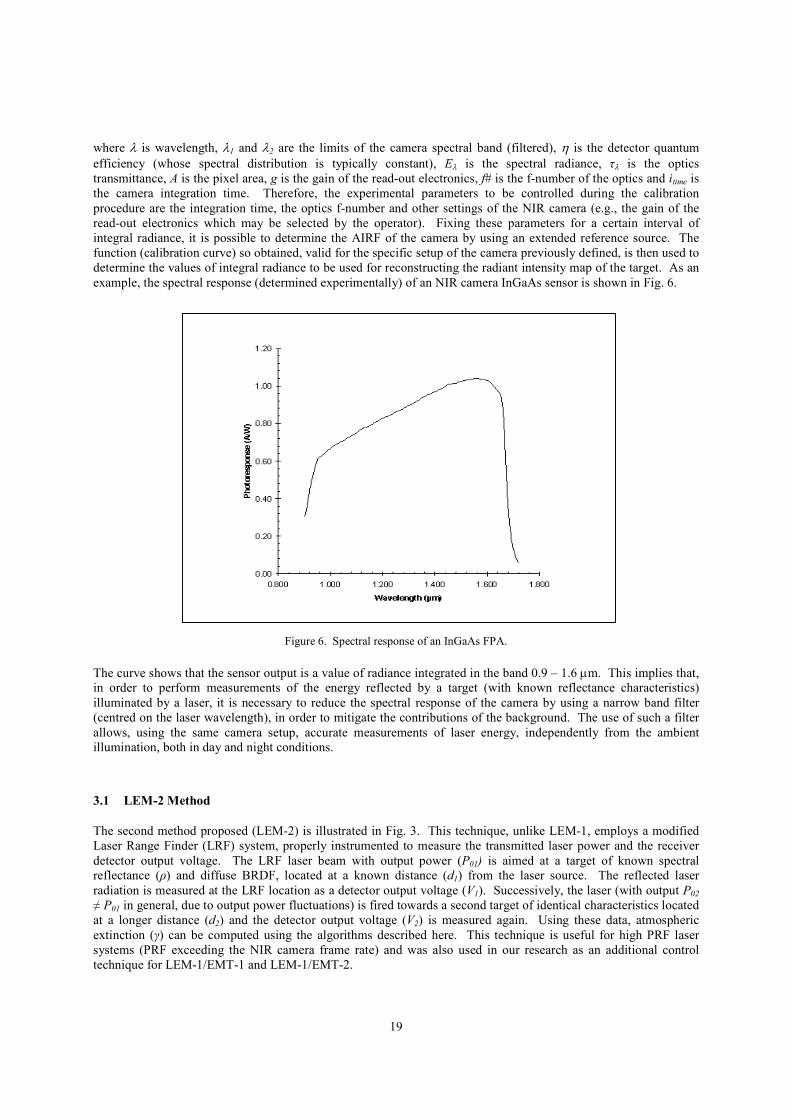
example, the spectral response (determined experimentally) of an NIR camera InGaAs sensor is shown in Fig. 6.
Figure 6. Spectral response of an InGaAs FPA.
The curve shows that the sensor output is a value of radiance integrated in the band 0.9 – 1.6 µm. This implies that,
in order to perform measurements of the energy reflected by a target (with known reflectance characteristics)
illuminated by a laser, it is necessary to reduce the spectral response of the camera by using a narrow band filter
(centred on the laser wavelength), in order to mitigate the contributions of the background. The use of such a filter
allows, using the same camera setup, accurate measurements of laser energy, independently from the ambient
illumination, both in day and night conditions.
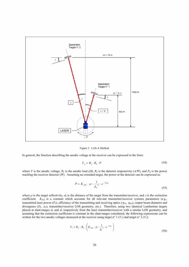
3.1 LEM-2 Method
The second method proposed (LEM-2) is illustrated in Fig. 3. This technique, unlike LEM-1, employs a modified
Laser Range Finder (LRF) system, properly instrumented to measure the transmitted laser power and the receiver
detector output voltage. The LRF laser beam with output power (P01) is aimed at a target of known spectral
reflectance (ρ) and diffuse BRDF, located at a known distance (d1) from the laser source. The reflected laser
radiation is measured at the LRF location as a detector output voltage (V1). Successively, the laser (with output P02
≠ P01 in general, due to output power fluctuations) is fired towards a second target of identical characteristics located
at a longer distance (d2) and the detector output voltage (V2) is measured again. Using these data, atmospheric
extinction (γ) can be computed using the algorithms described here. This technique is useful for high PRF laser
systems (PRF exceeding the NIR camera frame rate) and was also used in our research as an additional control
technique for LEM-1/EMT-1 and LEM-1/EMT-2.
20
LASER
Figure 3. LAS-A Method.
In general, the function describing the anodic voltage at the receiver can be expressed in the form:
PRRV SLA ⋅⋅= (54)
where V is the anodic voltage, RL is the anodic load (Ω), RS is the detector responsivity (A/W), and PR is the power
reaching the receiver detector (W). Assuming an extended target, the power at the detector can be expressed as:
02
2
0
1 d
SYS ed
KPγρ −⋅⋅⋅=
(55)
where ρ is the target reflectivity, d0 is the distance of the target from the transmitter/receiver, and γ is the extinction
coefficient. KSYS is a constant which accounts for all relevant transmitter/receiver systems parameters (e.g.,
transmitted laser power (P0), efficiency of the transmitting and receiving optics (ηTX, ηRX), output beam diameter and
divergence (DL, αT), transmitter/receiver LOS geometry, etc.). Therefore, using two identical Lambertian targets
placed at slant-ranges d1 and d2 respectively from the laser transmitter/receiver with a similar LOS geometry, and
assuming that the extinction coefficient is constant in the slant-ranges considered, the following expressions can be
written for the two anodic voltages measured at the receiver using target n° 1 (V1) and target n° 2 (V2):
⋅⋅⋅⋅⋅= − 12
2
1
1
1 d
SYSSL ed
KRRVγρ
(56)
21
⋅⋅⋅⋅⋅= − 22
2
2
2
1 d
SYSSL ed
KRRVγρ
(57)
It is reasonable to assume that, measuring the anodic voltages V1 and V2 , all system parameters remain constant,
except the transmitted laser power (P0) which may vary significantly in the time intervals where the two
measurement sessions are performed. With these assumptions, we can write the following expressions:
2
1
2
011
1
d
ePKV
dγ−
⋅⋅= (58)
2
2
2
022
2
d
ePKV
dγ−
⋅⋅= (59)
where P01 and P02 are the transmitted laser powers, and the factor K contains all constant terms. Therefore:
)(2
2
1
2
2
02
01
2
1 12 dded
d
P
P
V
V −⋅⋅= γ
(60)
Finally, we obtain:
⋅
⋅
⋅∆
=2
2
02
2
2
1
01
1
ln2
1
dP
V
dP
V
dγ
(61)
where the difference of the system to target slant-ranges (d1 - d2) has been replaced by the symbol ∆d. It should be
noted that all parameters contributing to the constant K do not affect the measurements (i.e., knowledge of these
parameters is not required if their value remains constant during the measurements performed on target n° 1 and n°
2). Obviously, the accuracy in the measurement of γ is affected by: 1) the error in measuring the distances d1 and d2;
2) the error in measuring the voltages V1 and V2; and 3) the error in measuring the powers P01 and P02. Therefore,
considering the errors relative to the measured parameters (σd1, σd2, σV1, σV2, σP01, σP02), we can write:
( ) ( )
2
1
22
12
2
2
2
22
22
2
2
02
2
2
01
2
22
2
2
2
1
2
2
2
12
020121
11
2
1
2
1
dd
ddd
d
PPdVVd
dd
PPVV
σ
γγσ
γγ
σσσσσ γ
⋅
+⋅
∆+⋅
+⋅
∆+
+
+⋅
∆+
+⋅
∆= (62)
Assuming that the error σd and the relative errors σV/V and σP0/P0 are the same for the measurements performed
with target n° 1 and target n° 2, we have:
⋅
++⋅
+⋅
∆+
+⋅
∆=
2
2
22
22
1
22
12
2
2
0
2
2
2
2
2 11
2
10
dd
dd
dPVd
ddPV σγ
σγ
γσσσ γ
(63)
Rearranging the terms, we obtain:
⋅
++⋅
+⋅+
+⋅⋅
∆=
2
2
22
22
1
22
1
2
2
0
2
2
211
2
110
dd
dd
PVd
ddPV σγ
σγ
γσσ
σγ (64)
Thus, it is evident that the error in the measurement of γ is strongly affected by the distance between the two targets.
For instance, in the case of laser system with transmitter/receiver parameters, σV/V = 5% and σPO/PO = 2%.
Assuming σd = 1 m, d1 = 800 m, ∆d = 100 m, d2 = 900 m, γ = 7×10⁻⁴
m-1
, from Eq. (31) we obtain a relative
22
measurement error σγ/γ of about 54%. Obviously, doubling the distance between the two targets (e.g, assuming ∆d
= 200 m and d2 = 1000 m), the estimated relative error would be 27% (half of the previous case). Assuming that the
laser platform and target coordinates can be determined with a σd ≤ 0.01, we obtain:
⋅
++⋅
+⋅>>>
+⋅
2
2
22
22
1
22
1
2
2
2
2
211
2
1
dd
dd
PV
dd
O
PV Oσ
γσ
γγ
σσ (65)
+⋅⋅
∆≅
2
2
2
2
2
11
O
PV
PVd
Oσσ
σ γ
(66)
Assuming ∆d = 1000 m, the estimated measurement error would be:
15-
2
2
2
2
103.812
11 −⋅=
+⋅⋅
∆≅ m
PVdO
PV Oσσ
σ γ
(67)
Since in general γ > 10-4 m-1, we obtain a maximum relative error σγ/γ of about 4%.
4. Experimental Results
In this section we present experimental results relative to the test activities performed using the proposed LEM-
1/EMT-2 technique (calibrated NIR camera). It should be noted that, during the initial phases of the test campaign,
some trials were performed with LEM-1/EMT-1 and LEM-1/EMT-2 from a range of 2 km and the results compared
with the LEM-2 measurements (d1 = 500 m, ∆d = 1500 m, d2 = 2000 m,). Using samples of 300 measurements, the
standard deviation of the observed differences was 3.6% for LEM-1/EMT-1 and 2.5% for LEM-1/EMT-2. The
dedicated LEM-1/EMT-2 experimental campaign presented here included both ground and flight test activities
performed with laser systems operating in the NIR at λ = 1064 nm (Nd:YAG) and λ = 1550 nm (Erbium-fibre).
During these test activities measurements were performed of horizontal and oblique/vertical path atmospheric
transmission up to altitudes of 22,000 ft AGL, in a large variety of atmospheric conditions.
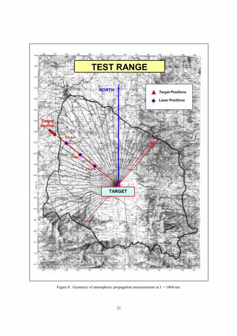
4.1 Propagation Trials at λλλλ = 1064 nm
Propagation trials at λ = 1064 nm were performed at the Air Force Laser Test Range in Sardinia (Italy). The laser
system was positioned along the target normal at a distance of 2.5 km, 4 km and 5.5 km. The target Mean Sea Level
(MSL) altitude was about 500 m and the maximum altitude difference between the laser transmitter and the target
was about 140 m at a distance of 5.5 km. The geometry of the λ = 1064 nm propagation tests performed at the range
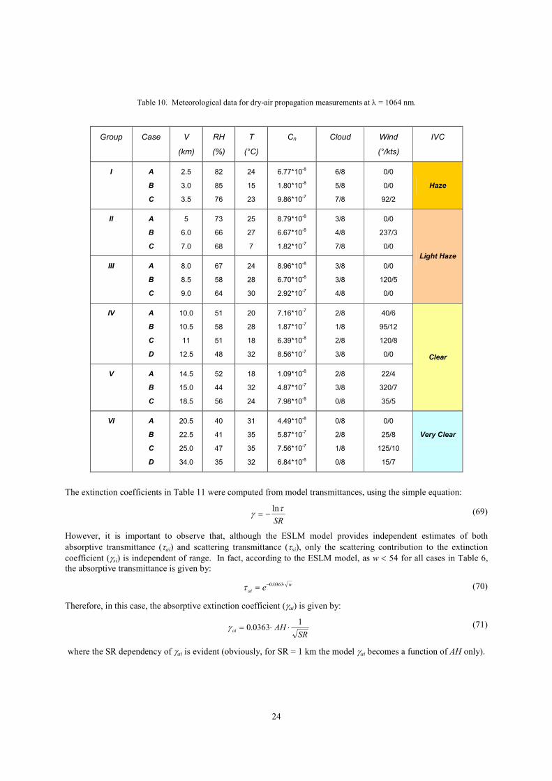
are shown in Fig. 8. Table 10 shows the relevant data describing the meteorological conditions in which the
atmospheric propagation measurements were performed (dry-air conditions). The various test cases have been
grouped for classes of visibility and the corresponding International Visibility Code (IVC) classes are reported.
When significant variations of T and/or RH were observed during the measurements, only the average values
calculated in the relevant time intervals have been reported. The prevailing wind direction/intensity during the
measurements is listed with respect to the laser to target slant-path (usual counter-clockwise convention). The
values of the Turbulence Structure Constant (Cn) were determined using the SCINTEC BLS900 laser scintillometer,
with a measurement baseline of 5 km between transmitter and receiver (along the target normal). For each case
listed in Table 10, a minimum of 25 energy measurements were performed (samples of 25 to 50 laser spot
measurements were used) using at least two of the laser system locations shown in Fig. 8. Dry-air extinction tests
were performed in all meteorological conditions listed in Table 11 only with a system to target slant-range (SR) of
2.5 km. With SR = 4 km and SR = 5.5 km, extinction tests were performed in a representative sub-set of dry-air
meteorological conditions. Rain extinction tests were not performed at λ = 1064 nm. Transmittance and extinction
coefficient values relative to the various test cases (i.e., meteorological conditions listed in Table 10), calculated
using the ESLM model with SR = 1 km, are listed in Table 11.
23
Figure 8. Geometry of atmospheric propagation measurements at λ = 1064 nm.
24
Table 10. Meteorological data for dry-air propagation measurements at λ = 1064 nm.
Group Case V
(km)
RH
(%)
T
(°C)
Cn Cloud Wind
(°/kts)
IVC
I A
B
C
2.5
3.0
3.5
82
85
76
24
15
23
6.77*10-8
1.80*10-8
9.86*10-7
6/8
5/8
7/8
0/0
0/0
92/2
Haze
II A
B
C
5
6.0
7.0
73
66
68
25
27
7
8.79*10-8
6.67*10-8
1.82*10-7
3/8
4/8
7/8
0/0
237/3
0/0
Light Haze
III A
B
C
8.0
8.5
9.0
67
58
64
24
28
30
8.96*10-8
6.70*10-8
2.92*10-7
3/8
3/8
4/8
0/0
120/5
0/0
IV A
B
C
D
10.0
10.5
11
12.5
51
58
51
48
20
28
18
32
7.16*10-7
1.87*10-7
6.39*10-8
8.56*10-7
2/8
1/8
2/8
3/8
40/6
95/12
120/8
0/0 Clear
V A
B
C
14.5
15.0
18.5
52
44
56
18
32
24
1.09*10-8
4.87*10-7
7.98*10-8
2/8
3/8
0/8
22/4
320/7
35/5
VI A
B
C
D
20.5
22.5
25.0
34.0
40
41
47
35
31
35
35
32
4.49*10-8
5.87*10-7
7.56*10-7
6.84*10-8
0/8
2/8
1/8
0/8
0/0
25/8
125/10
15/7
Very Clear
The extinction coefficients in Table 11 were computed from model transmittances, using the simple equation:
SR
τγ
ln−= (69)
However, it is important to observe that, although the ESLM model provides independent estimates of both
absorptive transmittance (τai) and scattering transmittance (τsi), only the scattering contribution to the extinction
coefficient (γsi) is independent of range. In fact, according to the ESLM model, as w < 54 for all cases in Table 6,
the absorptive transmittance is given by:
w
ai e ⋅−= 0363.0τ (70)
Therefore, in this case, the absorptive extinction coefficient (γai) is given by:
SR
AHai
10363.0 ⋅⋅=γ (71)
where the SR dependency of γai is evident (obviously, for SR = 1 km the model γai becomes a function of AH only).
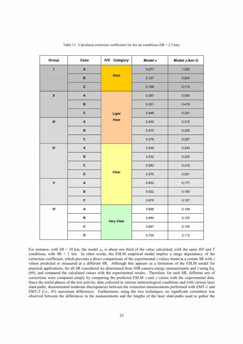
25
Table 11. Calculated extinction coefficients for dry-air conditions (SR = 2.5 km).
Group Case IVC Category Model ττττ Model γγγγ (km-1)
I
A
Haze
0.077 1.025
B 0.127 0,824
C 0.168 0,714
II A
Light
Haze
0.287 0,500
B 0.351 0,419
C 0.448 0,321
III A 0.455 0,315
B 0.470 0,302
C 0.476 0,297
IV A
Clear
0.549 0,240
B 0.532 0,252
C 0.583 0,216
D 0.575 0,221
V A 0.652 0,171
B 0.622 0,190
C 0.675 0,157
VI A
Very Clear
0.688 0,149
B 0.684 0,152
C 0.687 0,150
D 0.755 0,112
For instance, with SR = 10 km, the model γai is about one third of the value calculated, with the same RH and T
conditions, with SR = 1 km. In other words, the ESLM empirical model implies a range dependency of the
extinction coefficient, which prevents a direct comparisons of the experimental γ values found at a certain SR with γ values predicted or measured at a different SR. Although this appears as a limitation of the ESLM model for
practical applications, for all SR considered we determined from NIR-camera energy measurements and γ using Eq.
(69), and compared the calculated values with the experimental results. Therefore, for each SR, different sets of
corrections were computed simply by comparing the predicted ESLM τ and γ values with the experimental data.
Since the initial phases of the test activity, data collected in various meteorological conditions and with various laser
slant-paths, demonstrated moderate discrepancies between the extinction measurements performed with EMT-1 and
EMT-2 (i.e., 8% maximum difference). Furthermore, using the two techniques, no significant correlation was
observed between the differences in the measurements and the lengths of the laser slant-paths used to gather the
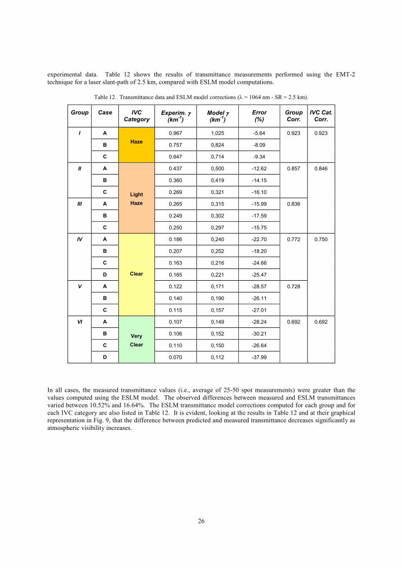
26
experimental data. Table 12 shows the results of transmittance measurements performed using the EMT-2
technique for a laser slant-path of 2.5 km, compared with ESLM model computations.
Table 12. Transmittance data and ESLM model corrections (λ = 1064 nm - SR = 2.5 km).
Group Case IVC Category
Experim. γγγγ (km
-1)
Model γγγγ (km
-1)
Error (%)
Group Corr.
IVC Cat. Corr.
I A
Haze
0.967 1,025 -5.64 0.923 0.923
B 0.757 0,824 -8.09
C 0.647 0,714 -9.34
II A
Light
Haze
0.437 0,500 -12.62 0.857 0.846
B 0.360 0,419 -14.15
C 0.269 0,321 -16.10
III A 0.265 0,315 -15.99 0.836
B 0.249 0,302 -17.59
C 0.250 0,297 -15.75
IV A
Clear
0.186 0,240 -22.70 0.772 0.750
B 0.207 0,252 -18.20
C 0.163 0,216 -24.66
D 0.165 0,221 -25.47
V A 0.122 0,171 -28.57 0.728
B 0.140 0,190 -26.11
C 0.115 0,157 -27.01
VI A
Very
Clear
0.107 0,149 -28.24 0.692 0.692
B 0.106 0,152 -30.21
C 0.110 0,150 -26.64
D 0.070 0,112 -37.99
In all cases, the measured transmittance values (i.e., average of 25-50 spot measurements) were greater than the
values computed using the ESLM model. The observed differences between measured and ESLM transmittances
varied between 10.52% and 16.64%. The ESLM transmittance model corrections computed for each group and for
each IVC category are also listed in Table 12. It is evident, looking at the results in Table 12 and at their graphical
representation in Fig. 9, that the difference between predicted and measured transmittance decreases significantly as
atmospheric visibility increases.
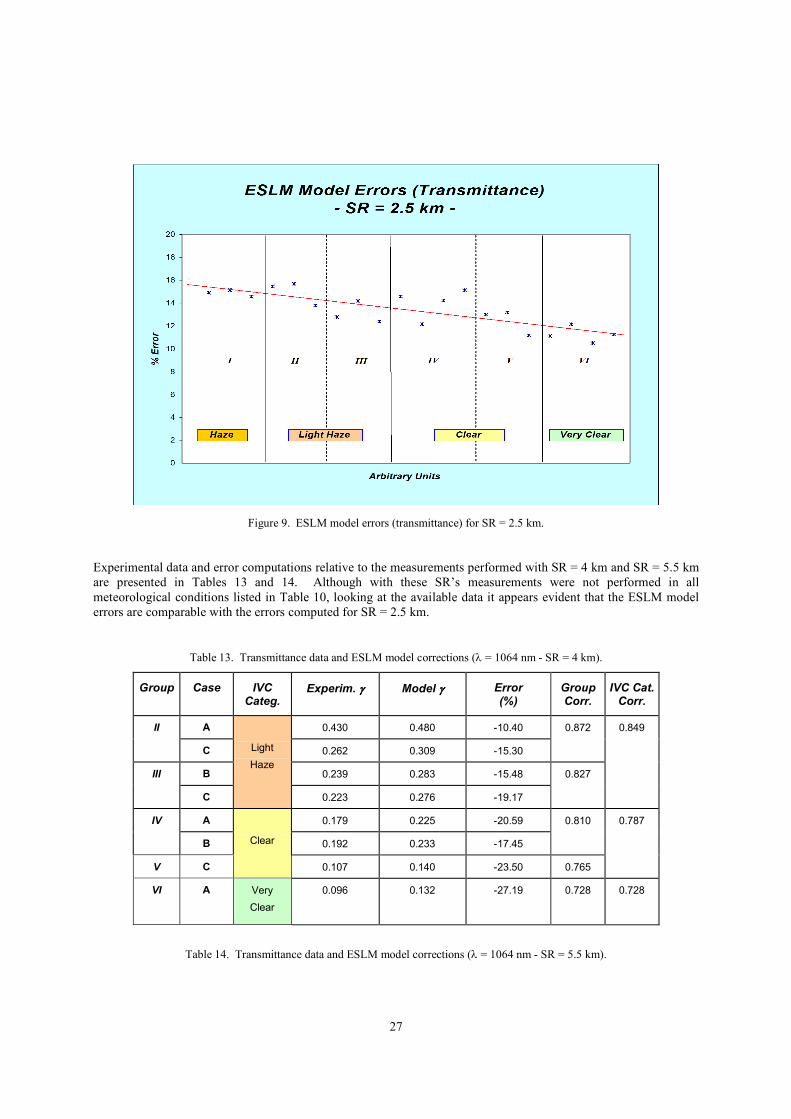
27
Figure 9. ESLM model errors (transmittance) for SR = 2.5 km.
Experimental data and error computations relative to the measurements performed with SR = 4 km and SR = 5.5 km
are presented in Tables 13 and 14. Although with these SR’s measurements were not performed in all
meteorological conditions listed in Table 10, looking at the available data it appears evident that the ESLM model
errors are comparable with the errors computed for SR = 2.5 km.
Table 13. Transmittance data and ESLM model corrections (λ = 1064 nm - SR = 4 km).
Group Case IVC Categ.
Experim. γγγγ Model γγγγ Error (%)
Group Corr.
IVC Cat. Corr.
II A
Light
Haze
0.430 0.480 -10.40 0.872 0.849
C 0.262 0.309 -15.30
III B 0.239 0.283 -15.48 0.827
C 0.223 0.276 -19.17
IV A
Clear
0.179 0.225 -20.59 0.810 0.787
B 0.192 0.233 -17.45
V C 0.107 0.140 -23.50 0.765
VI A Very
Clear
0.096 0.132 -27.19 0.728 0.728
Table 14. Transmittance data and ESLM model corrections (λ = 1064 nm - SR = 5.5 km).
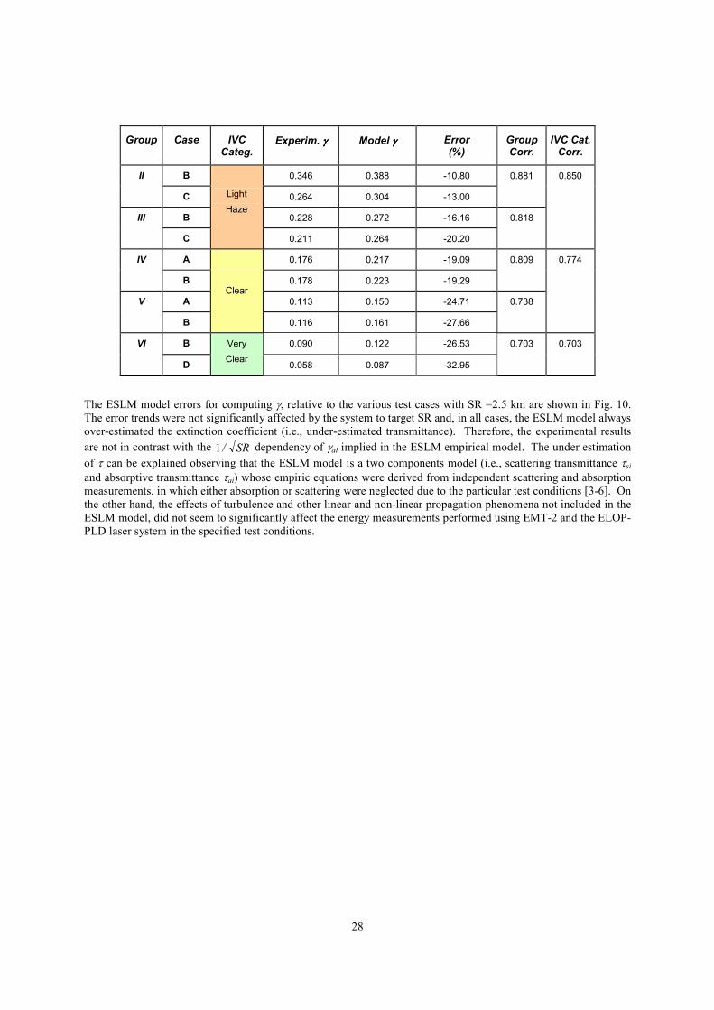
28
Group Case IVC Categ.
Experim. γγγγ Model γγγγ Error (%)
Group Corr.
IVC Cat. Corr.
II B
Light
Haze
0.346 0.388 -10.80 0.881 0.850
C 0.264 0.304 -13.00
III B 0.228 0.272 -16.16 0.818
C 0.211 0.264 -20.20
IV A
Clear
0.176 0.217 -19.09 0.809 0.774
B 0.178 0.223 -19.29
V A 0.113 0.150 -24.71 0.738
B 0.116 0.161 -27.66
VI B Very
Clear
0.090 0.122 -26.53 0.703 0.703
D 0.058 0.087 -32.95
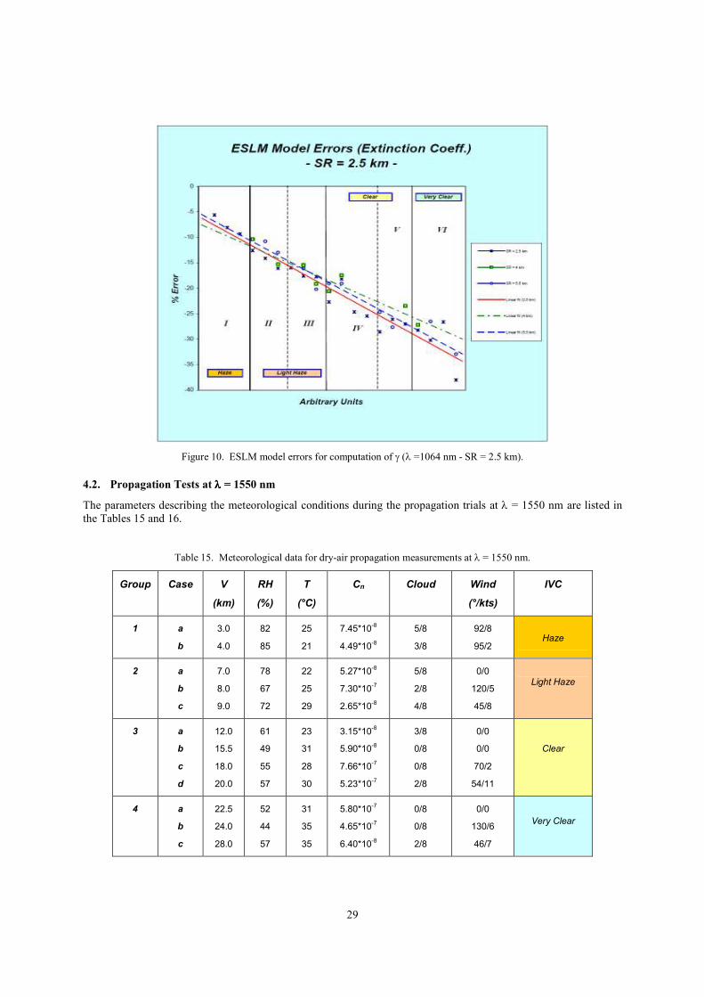
The ESLM model errors for computing γ, relative to the various test cases with SR =2.5 km are shown in Fig. 10.
The error trends were not significantly affected by the system to target SR and, in all cases, the ESLM model always
over-estimated the extinction coefficient (i.e., under-estimated transmittance). Therefore, the experimental results
are not in contrast with the SR/1 dependency of γai implied in the ESLM empirical model. The under estimation
of τ can be explained observing that the ESLM model is a two components model (i.e., scattering transmittance τsi
and absorptive transmittance τai) whose empiric equations were derived from independent scattering and absorption
measurements, in which either absorption or scattering were neglected due to the particular test conditions [3-6]. On
the other hand, the effects of turbulence and other linear and non-linear propagation phenomena not included in the
ESLM model, did not seem to significantly affect the energy measurements performed using EMT-2 and the ELOP-
PLD laser system in the specified test conditions.
29
Figure 10. ESLM model errors for computation of γ (λ =1064 nm - SR = 2.5 km).
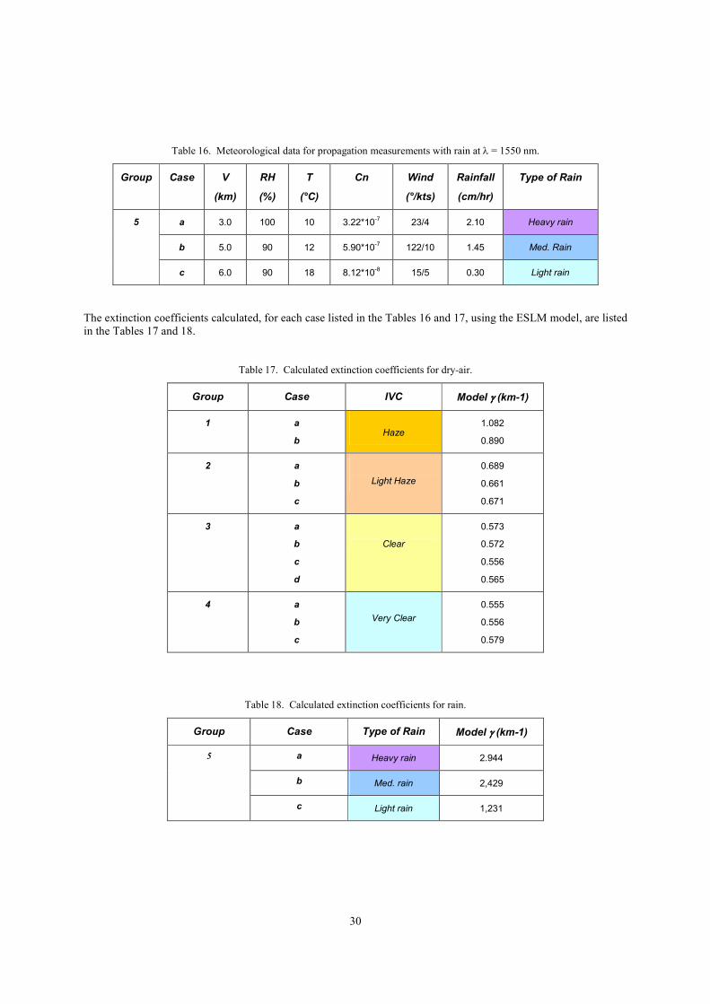
4.2. Propagation Tests at λλλλ = 1550 nm
The parameters describing the meteorological conditions during the propagation trials at λ = 1550 nm are listed in
the Tables 15 and 16.
Table 15. Meteorological data for dry-air propagation measurements at λ = 1550 nm.
Group Case V
(km)
RH
(%)
T
(°C)
Cn Cloud Wind
(°/kts)
IVC
1 a
b
3.0
4.0
82
85
25
21
7.45*10-8
4.49*10-8
5/8
3/8
92/8
95/2
Haze
2 a
b
c
7.0
8.0
9.0
78
67
72
22
25
29
5.27*10-8
7.30*10-7
2.65*10-8
5/8
2/8
4/8
0/0
120/5
45/8
Light Haze
3 a
b
c
d
12.0
15.5
18.0
20.0
61
49
55
57
23
31
28
30
3.15*10-8
5.90*10-8
7.66*10-7
5.23*10-7
3/8
0/8
0/8
2/8
0/0
0/0
70/2
54/11
Clear
4 a
b
c
22.5
24.0
28.0
52
44
57
31
35
35
5.80*10-7
4.65*10-7
6.40*10-8
0/8
0/8
2/8
0/0
130/6
46/7
Very Clear
30
Table 16. Meteorological data for propagation measurements with rain at λ = 1550 nm.
Group Case V
(km)
RH
(%)
T
(°C)
Cn Wind
(°/kts)
Rainfall
(cm/hr)
Type of Rain
5 a 3.0 100 10 3.22*10-7 23/4 2.10 Heavy rain
b 5.0 90 12 5.90*10-7 122/10 1.45 Med. Rain
c 6.0 90 18 8.12*10-8 15/5 0.30 Light rain
The extinction coefficients calculated, for each case listed in the Tables 16 and 17, using the ESLM model, are listed
in the Tables 17 and 18.
Table 17. Calculated extinction coefficients for dry-air.
Group Case IVC Model γγγγ (km-1)
1 a
b
Haze 1.082
0.890
2 a
b
c
Light Haze
0.689
0.661
0.671
3 a
b
c
d
Clear
0.573
0.572
0.556
0.565
4 a
b
c
Very Clear
0.555
0.556
0.579
Table 18. Calculated extinction coefficients for rain.
Group Case Type of Rain Model γγγγ (km-1)
5 a Heavy rain 2.944
b Med. rain 2,429
c Light rain 1,231
31
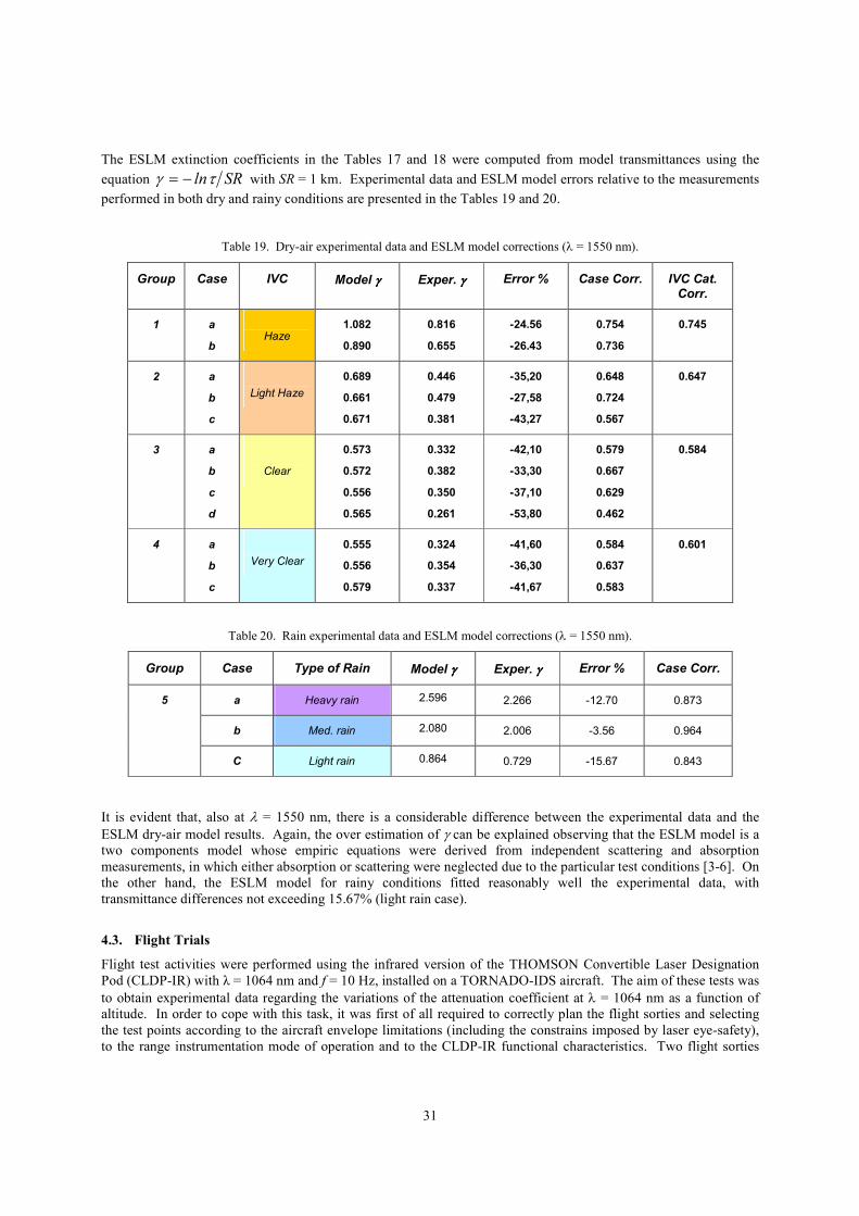
The ESLM extinction coefficients in the Tables 17 and 18 were computed from model transmittances using the
equation SRlnτγ −= with SR = 1 km. Experimental data and ESLM model errors relative to the measurements
performed in both dry and rainy conditions are presented in the Tables 19 and 20.
Table 19. Dry-air experimental data and ESLM model corrections (λ = 1550 nm).
Group Case IVC Model γγγγ Exper. γγγγ Error % Case Corr. IVC Cat. Corr.
1 a
b
Haze 1.082
0.890
0.816
0.655
-24.56
-26.43
0.754
0.736
0.745
2 a
b
c
Light Haze
0.689
0.661
0.671
0.446
0.479
0.381
-35,20
-27,58
-43,27
0.648
0.724
0.567
0.647
3 a
b
c
d
Clear
0.573
0.572
0.556
0.565
0.332
0.382
0.350
0.261
-42,10
-33,30
-37,10
-53,80
0.579
0.667
0.629
0.462
0.584
4 a
b
c
Very Clear
0.555
0.556
0.579
0.324
0.354
0.337
-41,60
-36,30
-41,67
0.584
0.637
0.583
0.601
Table 20. Rain experimental data and ESLM model corrections (λ = 1550 nm).
Group Case Type of Rain Model γγγγ Exper. γγγγ Error % Case Corr.
5
a Heavy rain 2.596 2.266 -12.70 0.873
b Med. rain 2.080 2.006 -3.56 0.964
C Light rain 0.864 0.729 -15.67 0.843
It is evident that, also at λ = 1550 nm, there is a considerable difference between the experimental data and the
ESLM dry-air model results. Again, the over estimation of γ can be explained observing that the ESLM model is a
two components model whose empiric equations were derived from independent scattering and absorption
measurements, in which either absorption or scattering were neglected due to the particular test conditions [3-6]. On
the other hand, the ESLM model for rainy conditions fitted reasonably well the experimental data, with
transmittance differences not exceeding 15.67% (light rain case).
4.3. Flight Trials
Flight test activities were performed using the infrared version of the THOMSON Convertible Laser Designation
Pod (CLDP-IR) with λ = 1064 nm and f = 10 Hz, installed on a TORNADO-IDS aircraft. The aim of these tests was
to obtain experimental data regarding the variations of the attenuation coefficient at λ = 1064 nm as a function of
altitude. In order to cope with this task, it was first of all required to correctly plan the flight sorties and selecting
the test points according to the aircraft envelope limitations (including the constrains imposed by laser eye-safety),
to the range instrumentation mode of operation and to the CLDP-IR functional characteristics. Two flight sorties
32
were executed in days with visibility in excess of 15 km, including four dive manoeuvres at 45°, 35°, 25° and 15°
respectively. The dive profiles envelopes are described in the Table 21.
Table 21. Flight profiles envelopes for propagation flight trials.
Profile Envelope
20° Dive 30° Dive 40° Dive 50° Dive
Alt. Dist. Alt. Dist. Alt. Dist. Alt. Dist.
Top 14000 ft 12.5 km 19000 ft 11.5 km 20000 ft 9.5 km 22000 ft 8.5 km
Bottom 6000 ft 5.5 km 7000 ft 4 km 8000 ft 4 km 8000 ft 3.5 km
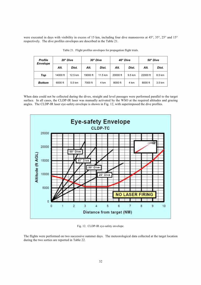
When data could not be collected during the dives, straight and level passages were performed parallel to the target
surface. In all cases, the CLDP-IR laser was manually activated by the WSO at the required altitudes and grazing
angles. The CLDP-IR laser eye-safety envelope is shown in Fig. 12, with superimposed the dive profiles.
Fig. 12. CLDP-IR eye-safety envelope.
The flights were performed on two successive summer days. The meteorological data collected at the target location
during the two sorties are reported in Table 22.
33
Table 22. Meteorological data relative to propagation flight trials.
Sortie Visibility (km)
Rel. Humidity (%)
Temperature (°C)
Wind (°/kts)
Cloud
1 16 km 57% 35°C 120/7 0/8
2 18 km 54% 32°C 0/0 2/8
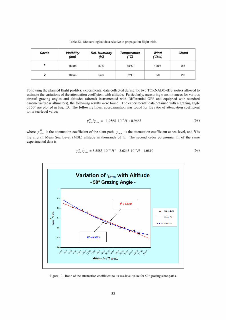
Following the planned flight profiles, experimental data collected during the two TORNADO-IDS sorties allowed to
estimate the variations of the attenuation coefficient with altitude. Particularly, measuring transmittances for various
aircraft grazing angles and altitudes (aircraft instrumented with Differential GPS and equipped with standard
barometric/radar altimeters), the following results were found. The experimental data obtained with a grazing angle
of 50° are plotted in Fig. 13. The following linear approximation was found for the ratio of attenuation coefficient
to its sea-level value:
9663.0109568.1 5 +⋅−= − Hatm
H
atm γγ (68)
where H
atmγ is the attenuation coefficient of the slant-path, atmγ is the attenuation coefficient at sea-level, and H is
the aircraft Mean Sea Level (MSL) altitude in thousands of ft. The second order polynomial fit of the same
experimental data is:
0810.1106243.3105583.55210 +⋅−⋅= −−HHatm
H
atm γγ (69)
Figure 13. Ratio of the attenuation coefficient to its sea-level value for 50° grazing slant-paths.
34
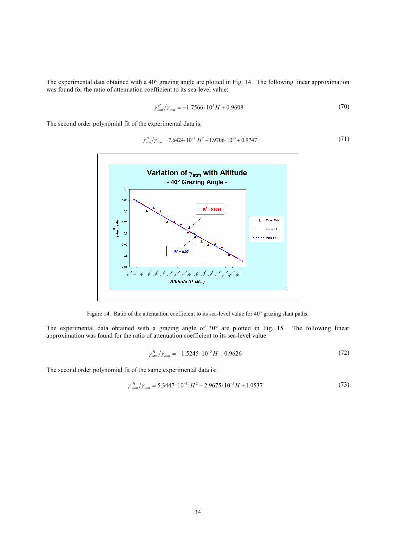
The experimental data obtained with a 40° grazing angle are plotted in Fig. 14. The following linear approximation
was found for the ratio of attenuation coefficient to its sea-level value:
9608.0107566.1 5 +⋅−= Hatm
H
atm γγ (70)
The second order polynomial fit of the experimental data is:
9747.0109706.1106424.7 5211 +⋅−⋅= −− Hatm
H
atm γγ (71)
Figure 14. Ratio of the attenuation coefficient to its sea-level value for 40° grazing slant paths.
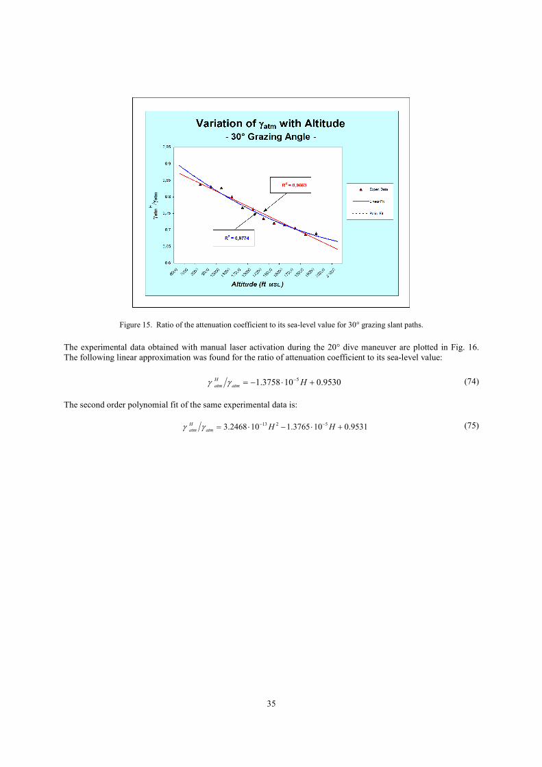
The experimental data obtained with a grazing angle of 30° are plotted in Fig. 15. The following linear
approximation was found for the ratio of attenuation coefficient to its sea-level value:
9626.0105245.1 5 +⋅−= − Hatm
H
atm γγ (72)
The second order polynomial fit of the same experimental data is:
0537.1109675.2103447.5 5210 +⋅−⋅= −− HHatm
H
atm γγ (73)
35
Figure 15. Ratio of the attenuation coefficient to its sea-level value for 30° grazing slant paths.
The experimental data obtained with manual laser activation during the 20° dive maneuver are plotted in Fig. 16.
The following linear approximation was found for the ratio of attenuation coefficient to its sea-level value:
9530.0103758.1 5 +⋅−= − Hatm
H
atm γγ (74)
The second order polynomial fit of the same experimental data is:
9531.0103765.1102468.3 5213 +⋅−⋅= −− HHatm
H
atm γγ (75)
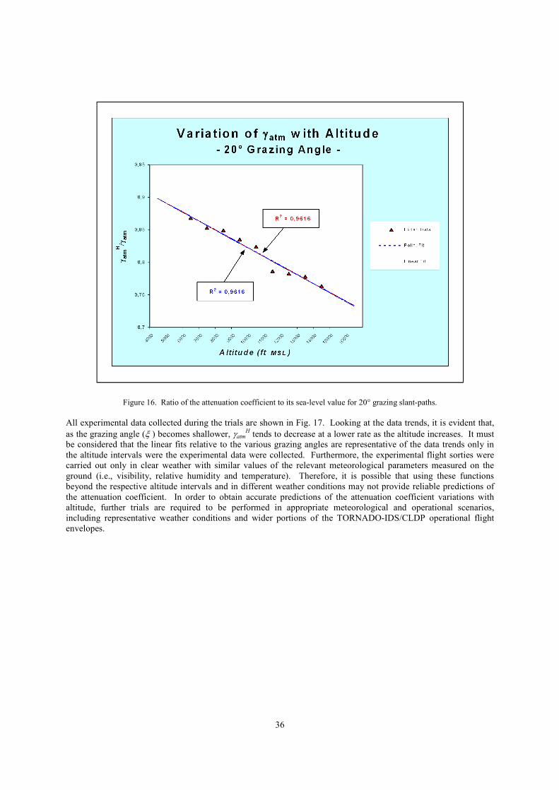
36
Figure 16. Ratio of the attenuation coefficient to its sea-level value for 20° grazing slant-paths.
All experimental data collected during the trials are shown in Fig. 17. Looking at the data trends, it is evident that,
as the grazing angle (ξ ) becomes shallower, γatmH tends to decrease at a lower rate as the altitude increases. It must
be considered that the linear fits relative to the various grazing angles are representative of the data trends only in
the altitude intervals were the experimental data were collected. Furthermore, the experimental flight sorties were
carried out only in clear weather with similar values of the relevant meteorological parameters measured on the
ground (i.e., visibility, relative humidity and temperature). Therefore, it is possible that using these functions
beyond the respective altitude intervals and in different weather conditions may not provide reliable predictions of
the attenuation coefficient. In order to obtain accurate predictions of the attenuation coefficient variations with
altitude, further trials are required to be performed in appropriate meteorological and operational scenarios,
including representative weather conditions and wider portions of the TORNADO-IDS/CLDP operational flight
envelopes.
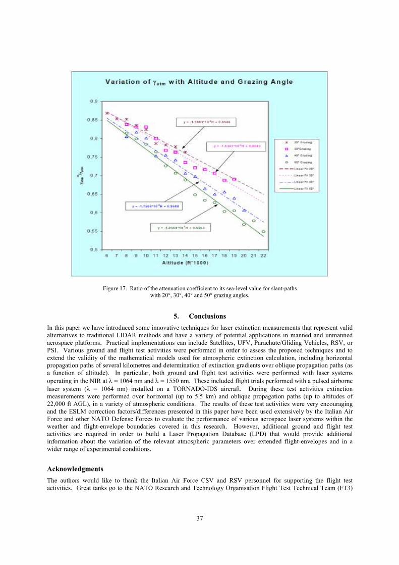
37
Figure 17. Ratio of the attenuation coefficient to its sea-level value for slant-paths
with 20°, 30°, 40° and 50° grazing angles.
5. Conclusions
In this paper we have introduced some innovative techniques for laser extinction measurements that represent valid
alternatives to traditional LIDAR methods and have a variety of potential applications in manned and unmanned
aerospace platforms. Practical implementations can include Satellites, UFV, Parachute/Gliding Vehicles, RSV, or
PSI. Various ground and flight test activities were performed in order to assess the proposed techniques and to
extend the validity of the mathematical models used for atmospheric extinction calculation, including horizontal
propagation paths of several kilometres and determination of extinction gradients over oblique propagation paths (as
a function of altitude). In particular, both ground and flight test activities were performed with laser systems
operating in the NIR at λ = 1064 nm and λ = 1550 nm. These included flight trials performed with a pulsed airborne
laser system (λ = 1064 nm) installed on a TORNADO-IDS aircraft. During these test activities extinction
measurements were performed over horizontal (up to 5.5 km) and oblique propagation paths (up to altitudes of
22,000 ft AGL), in a variety of atmospheric conditions. The results of these test activities were very encouraging
and the ESLM correction factors/differences presented in this paper have been used extensively by the Italian Air
Force and other NATO Defense Forces to evaluate the performance of various aerospace laser systems within the
weather and flight-envelope boundaries covered in this research. However, additional ground and flight test
activities are required in order to build a Laser Propagation Database (LPD) that would provide additional
information about the variation of the relevant atmospheric parameters over extended flight-envelopes and in a
wider range of experimental conditions.
Acknowledgments
The authors would like to thank the Italian Air Force CSV and RSV personnel for supporting the flight test
activities. Great tanks go to the NATO Research and Technology Organisation Flight Test Technical Team (FT3)
38
for their expert advice and support. Many thanks go to the personnel of SELEX and LOT-ORIEL for their support
to the laser test range program.
References
[1] Weichel H., “Laser Beam Propagation in the Atmosphere.” SPIE Optical Engineering Press. Second Printing
(1990).
[2] Hudson R.D., [Infrared Systems Engineering]. Wiley & Sons (1969).
[3] Elder T. and Strong J., “The Infrared Transmission of Atmospheric Windows.” J. Franklin Institute 255 – 189
(1953).
[4] Langer R.M., Signal Corps Report n° DA-36-039-SC-72351 (1957).
[5] Middleton W.E.K., “Vision Through the Atmosphere.” University of Toronto Press (1952).
[6] Middleton W.E.K., “Vision Through the Atmosphere.” Handbuch der Physik 48. Geophysics 2. Springer,
Berlin (1957).
[7] Kneizys F.X., Shuttle E.P., Abreau L.W., Chetwynd J.H., Anderson G.P., Gallery W.O., Selby J.E.A., and
Clough S.A., “Users Guide to LOWTRAN 7.” Air Force Geophysical Laboratory Report AFGL-TR-88-0177.
Hansom AFB (1988).
[8] Holst G.C., [Electro-Optical Imaging System Performance], SPIE Optical Engineering Press. Bellingham,
Washington USA (1995).
[9] Gebhardt F.G., “High Power Laser Propagation.” Applied Optics – Vol. 15, p. 1479 (1976).
[10] Rodgers C.D., “Inverse Methods for Atmospheric Sounding: Theory and Practice.” Atmos. Oceanic Planet.
Phys. – Vol. 2 (p. 238). World Science. River Edge, NJ (2000).
[11] Veselovskii I., Kolgotin A., Griaznov V., Müller D., Franke K., and Whiteman D., “Inversion of
multiwavelength Raman lidar data for retrieval of bimodal aerosol size distribution.” Appl. Optics – Vol. 43,
pp. 1180-1195 (2004).
[12] Müller D., Wagner F., Wandinger U., Ansmann A., Wendisch M., Althausen D., and Hoyningen-Huene von
W., “Microphysical particle parameters from extinction and backscatter lidar data by inversion with
regularization: Experiment.” Appl. Optics – Vol. 39, pp. 1879-1892 (2000).
[13] Abshire J.B., Riris H., Allan G.R., Weaver C.J., MAO J., Sun X., Hasselbrack W.E., Kawar R. and Biraud S.,
"Pulsed airborne lidar measurements of atmospheric CO2 column absorption." Tellus Journal - International
Meteorological Institute in Stockholm (2010).
[14] Krainak, M.A, Andrews, A. E., Allan, G. R., Burris, J. F., Riris, H. and co-authors, "Measurements of
atmospheric CO2 over a horizontal path using a tunable-diode-laser and erbium-fiber-amplifier at 1572 nm.”
Proceedings of the Conference on Lasers and Electro-Optics/Quantum Electronics and Laser Science.
Technical Digest, Optical Society of America, paper CTuX4, 878–881, ISBN: 1-55752-748-2 (2003).
[15] Riris, H., Abshire, J., Allan, G., Burris, J., Chen, J. and co-authors, "A laser sounder for measuring atmospheric
trace gases from space." Proc. SPIE 6750, 67500U, doi:10.1117/12.737607 (2007).
[16] Allan G. R., Riris, H., Abshire J. B., Sun X., Wilson E. and co-authors, "Laser sounder for active remote
sensing measurements of CO2 concentrations." Proceedings of the 2008 IEEE Aerospace Conference. IEEE,
Big Sky, MT. 1534–1540, doi:10.1109/AERO.2008.4526387 (2008).
[17] Amediek, A., Fix, A. Ehret, G. Caron, J. and Durand, Y., "Airborne lidar reflectance measurements at 1.57 um
in support of the A-SCOPE mission for atmospheric CO2." Atmos. Meas. Tech. Discuss. 2, 1487–1536
(2009).