
NOTE TO USERS
This reproduction is the best copy available.
UMI*

Color and Luminance Correction and Calibration System for
LED Video Screens
Mohammad Al-Mulazem
A Thesis
in
The Department
of
Electrical and Computer Engineering
Presented in Partial Fulfillment of the Requirements
for the Degree of Master of Applied Science (Electrical & Computer Engineering)
at
Concordia University
Montreal, Quebec, Canada
July 2009
© Mohammad Al-Mulazem, 2009
1*1 Library and Archives Canada
Published Heritage Branch
395 Wellington Street Ottawa ON K1A 0N4 Canada
Bibliotheque et Archives Canada
Direction du Patrimoine de I'edition
395, rue Wellington Ottawa ON K1A 0N4 Canada
Your file Votre reference ISBN: 978-0-494-63154-6 Our file Notre reference ISBN: 978-0-494-63154-6
NOTICE: AVIS:
The author has granted a nonexclusive license allowing Library and Archives Canada to reproduce, publish, archive, preserve, conserve, communicate to the public by telecommunication or on the Internet, loan, distribute and sell theses worldwide, for commercial or noncommercial purposes, in microform, paper, electronic and/or any other formats.
L'auteur a accorde une licence non exclusive permettant a la Bibliotheque et Archives Canada de reproduce, publier, archiver, sauvegarder, conserver, transmettre au public par telecommunication ou par I'lntemet, preter, distribuer et vendre des theses partout dans le monde, a des fins commerciales ou autres, sur support microforme, papier, electronique et/ou autres formats.
The author retains copyright ownership and moral rights in this thesis. Neither the thesis nor substantial extracts from it may be printed or otherwise reproduced without the author's permission.
L'auteur conserve la propriete du droit d'auteur et des droits moraux qui protege cette these. Ni la these ni des extraits substantiels de celle-ci ne doivent §tre imprimes ou autrement reproduits sans son autorisation.
In compliance with the Canadian Privacy Act some supporting forms may have been removed from this thesis.
Conformement a la loi canadienne sur la protection de la vie privee, quelques formulaires secondaires ont ete enleves de cette these.
While these forms may be included in the document page count, their removal does not represent any loss of content from the thesis.
Bien que ces formulaires aient inclus dans la pagination, il n'y aura aucun contenu manquant.
1+1
Canada
ABSTRACT
Color and Luminance Correction and Calibration System for LED Video Screens
Mohammad Al-Mulazem
Recent years have seen a surge in the popularity of Light emitting diode (LED) video
screens, which have come to be a critical part of how the world of show business and
corporate events are seen by their audiences. LED video screens are bright, visually
attractive, can stand severe weather conditions, and consume far less power than CRT
technology. In LED screens technology, pixels are composed of three primary LED
colors: red, green, and blue (RGB). Using the primary colored LEDs provide the ability
to generate variety of color hues, saturations and values. However, the RGB LEDs in the
screen's pixels have different luminance and color due to the LEDs themselves. These
differences seriously destroy the white balance of the LED pixels and modules, and make
the picture color aberration, blotchy and patchy. To overcome these problems, different
techniques and methodologies has been proposed in the literature. The main drawbacks
of these techniques are the cost-effectiveness in the sense they provide mediocre
resolution. In this thesis, a new and cost-effective methodology and technique is proposed
to correct the color and the luminance of LED video screens while maintaining a high
quality and high resolution image display. Also, a new developed algorithm is proposed
to fit different color and brightness calibration purposes. The proposed algorithm is based
on the CIE Commission Internationale de l'Eclairage standards. The technique and
methodology have been implemented, in collaboration with LSI SACO Technologies Inc.,
using fully automated robotic spectrometer system and achieved the targeted goals.
i i i

CONCORDIA UNIVERSITY
School of Graduate Studies
This is to certify that the thesis prepared
By: Mohammad Al-Mulazem
Entitled: Color and Luminance Correction and Calibration System for
LED Video Screens
and submitted in partial fulfillment of the requirements for the degree of
Master of Applied Science (Electrical & Computer Engineering)
complies with the regulations of this University and meets the accepted standards
with respect to originality and quality.
Signed by the final examining committee:
Dr. Amir G. Aghdam
Dr. Ibrahim G. Hassan
Dr. Luiz A.C. Lopes
Dr. Otmane Ait Mohamed
Approved by
Chair of the ECE Department
2009
Dean of Engineering

ACKNOWLEDGEMENTS
First of all, I would like to express my appreciation to my supervisor Dr. Otmane Ait
Mohamed for believing in me and for his continuous support during my research. I am
also very thankful to my supervisor at LSI SACO Technologies Mr. Bassam Jalbout for
giving me the opportunity to do my Master's project at LSI SACO, and to Marc
Morrisseau for his continuous support, guidance, and feedback on the research project.
My sincere appreciation to the Fonds Quebecois de la Recherche sur la Nature et
la Technologie (FQRNT) and the Natural Sciences and Engineering Research Council of
Canada (NSERC) which have granted me the Industrial Innovation Scholarship at
Concordia University.
I would like to thank Suliman Albasheir and Mohannad El-Jayousi for their time
and valuable help during my thesis writing. Finally, my sincere thanks and deepest
appreciation go out to my parents, Adalah and Nihad, and my wife Sawsan for their
affection, love, support, encouragement, and prayers to success in my missions.
IV
This thesis is dedicated to
My Mother, My Father, My Wife
and
My Daughter Jana
v
TABLE OF CONTENTS
LIST OF FIGURES ix
LIST OF TABLES xiii
LIST OF NOMENCLATURE xiv
LIST OF ACRONYMS xv
1 Introduction 1
1.1 Motivation 1
1.2 Uniformity problems in LED screens 2
1.3 Proposed Solution 4
1.4 Related Work 6
1.5 Thesis Contribution 8
1.6 Thesis Outline 9
2 Preliminaries 10
2.1 LED video screen 10
2.1.1 LED pixel 11
2.1.2 Properties of LEDS 12
2.1.3 LED driver 15
2.1.4 PWM dimming 16
2.1.5 Matrix controller 17
2.2 Light and Color 19
2.2.1 Color perception and Color space 20
vi
2.3 CIE color system 22
2.3.1 CIE color matching functions 24
2.3.2 CIE XYZ tristimulus 24
2.3.3 CIE 1931 Chromaticity coordinates 25
2.3.4 CIE 1976 u'v' 26
2.4 Color Gamut 29
2.5 Additive Color Mixture 30
2.5.1 Grassmann's laws of additive color mixture 30
2.5.2 Newton's 'Centre of Gravity' Law of additive color mixing 31
2.5.3 Additive Color Mixing with CIE 32
2.6 PWM Correction Methodology 33
3 Correction and Calibration Algorithms 36
3.1 Introduction 36
3.2 Luminance Calibration Algorithm 36
3.3 Color Correction Algorithm 43
3.4 Proposed Methodologies 53
3.4.1RGBW Color and W Luminance 54
3.4.2 W Luminance and Color 56
3.4.3 RGB Color and Luminance 59
3.4.4 RGB Luminance 61
3.4.5 Achromatic Point 61
3.5 Image Quality and Resolution 62
vii

3.6 Summary 65
4 Correction and Calibration Experimantal Setup 66
4.1 Introduction 66
4.2 System Description ; 66
4.2.1 Robotic Spectrometer System 67
4.2.2 Correction Software 69
4.3 Color and Luminance Correction and Calibration Process 77
4.4 Summary 79
5 Experimental Results 80
5.1 Experiments Set Up 80
5.2 RGBW Color and W Luminance Experiment 81
5.3 RGB Color and Luminance Experiment 91
5.4 RGB Luminance Experiment 101
5.5 Discussion 108
6 Conclusions and Future Work I l l
6.1 Conclusions I l l
6.2 Future Work 112
Bibliography 113
Appendix 1 118
viii
LIST OF FIGURES
1.1 LED Pixels uniformity problem 3
1.2 Red, Green and Blue LEDs luminance decay with usage 4
2.1 LED Video Screen and LED Matrix 10
2.2 LED Matrix Structure 11
2.3 LED Matrix Pixel 12
2.4 (a) Broad-band spectral, (b) monochromatic, (c) quasi-monochromatic 13
2.5 Irradiance Mode 13
2.6 Forward current vs. Relative Luminosity graph for Blue LED 14
2.7 Forward current vs. Chromaticity Coordinates graph for Blue LED 15
2.8 Illustrative 3-channel LED Driver Block Diagram 15
2.9 Illustrative diagram for LED brightness control stages 16
2.10 Pulse Width Modulation 17
2.11 Illustrative block diagram of LED matrix controller 18
2.12 Visible spectrums 19
2.13 Spectral Power Distribution (SPD) for white LED 20
2.14 CIE 1931 Chromaticity Diagram 23
2.15 CLE color matching functions 24
2.16 MacAdam ellipses. The axes of plotted ellipses are 10 times their actual lengths... 27
2.17 1976 CIE u'v' chromaticity diagram 28
2.18 Color Gamuts 29
2.19 Newton's color wheel 31
ix
2.20 Red coefficients before and after correction 34
2.21 Full LED pixel correction coefficients 35
3.1 Luminance and Color Coordinates measuring procedure for red LED 38
3.2 Current vs. Luminosity (Example) 39
3.3 Light and measure (Ci, Yi) 40
3.4 Light and measure (C2, Y2) 40
3.5 Light and measure (C3, Y3) 41
3.6 Light and measure (Qarget, Ytarget) 41
3.7 Luminance calibration process flowchart 42
3.8 RGB LEDs luminance and color values 42
3.0 RGB LEDs luminance and color values 43
3.10 The color C can be matched by an additive mixture of the colors A & B 44
3.11 The color W can be matched by an additive mixture of the colors R, G, & B 45
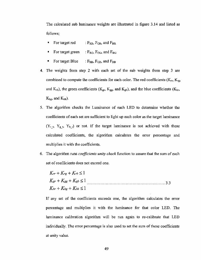
3.12 Saturated red, green, blue, and white measuring 47
3.13 Red, green and blue luminance weights (FR, FG, and FB) 47
3.14 Sub-luminance weights for target red, green and blue 48
3.15 Full LED pixel correction coefficients 50
3.16 Out of Gamut function 51
3.17 Color Correction algorithm flowchart 52
3.18 (FR t , FG_t and FBJ) according to (Wtarget) 55
3.19 FR, F G and FB according to WmeaSured 56
3.20 (FRR, FGG and FBB) according to (Wtarget) 57
3.21 LED pixel correction coefficients for W color and luminance methodology 58
x

3.22 LED pixel correction coefficients for RGBW color and W luminance methodology example 63
3.23 LED pixel correction coefficients for RGB color and luminance methodology example 64
4.1 Robot JR2500 by Janome 67
4.2 Spectrometer SPM-002-A by Photon Control 68
4.3 Light measuring path inside the spectrometer 68
4.4 Robotic Spectrometer system 69
4.5 Software classes 70
4.6 Software main page 71
4.7 Software Robot tab 71
4.8 Software Matrix Controller tab 72
4.9 Software Spectrometer tab 73
4.10 Software Pixel Control tab 75
4.11 Illustrative example for adapting exposure steps 76
4.12 CCD different exposure timing; (a) Low Exposure, (b) good exposure, (c) over exposed 76
4.13 Proposed Methodology Flowchart 78
5.1 Red Corrected and Default Color & Luminance Parameters Chart [RGBW Color and W luminance methodology] 88
5.2 Green Corrected and Default Color & Luminance Parameters Chart [RGBW Color and W luminance methodology] 88
5.3 Blue Corrected and Default Color & Luminance Parameters Chart [RGBW Color and W luminance methodology] 89
5.4 White Corrected and Default Color & Luminance Parameters Chart [RGBW Color and W luminance methodology] 89
XI

5.5 Red, Green, Blue and White Corrected and Default Color Coordinates Chart [RGBW Color and W luminance methodology] 90
5.6 Red Corrected and Default Color & Luminance Parameters Chart [RGB Color and Luminance methodology] 98
5.7 Green Corrected and Default Color & Luminance Parameters Chart [RGB Color and Luminance methodology] 98
5.8 Blue Corrected and Default Color & Luminance Parameters Chart [RGB Color and Luminance methodology] 99
5.9 White Corrected and Default Color & Luminance Parameters Chart [RGB Color and Luminance methodology] 99
5.10 Red, Green, Blue and White Corrected and Default Color Coordinates Chart [RGB Color and Luminance methodology] 100
5.11 Red Calibrated and Default Color & Luminance Parameters Chart [RGB Luminance methodology] 105
5.12 Green Calibrated and Default Color & Luminance Parameters Chart [RGB Luminance methodology] 105
5.13 Blue Calibrated and Default Color & Luminance Parameters Chart [RGB Luminance methodology] 106
5.14 White Calibrated and Default Color & Luminance Parameters Chart [RGB Luminance methodology] 106
5.15 Red, Green, Blue and White Calibrated and Default Color Coordinates Chart [RGB Luminance methodology] 107
xii

LIST OF TABLES
3.1 Methodologies efficiencies 65
5.1 Default, Calibrated, and Corrected Color coordinates and Luminance [RGBW Color and W Luminance] 82
5.2 Minimum, Maximum, and Average Color coordinates and Luminance [RGBW Color and W Luminance] 84
5.3 Coefficients and usage efficiency [RGBW Color and W Luminance] 85
5.4 Usage efficiency summary [RGBW Color and W Luminance] 87
5.5 Default, Calibrated, and Corrected Color coordinates and Luminance [RGB Color and Luminance] 92
5.6 Minimum, Maximum, and Average Color coordinates and Luminance [RGB Color and Luminance] 94
5.7 Coefficients and Usage efficiency [RGB Color and Luminance] 95
5.8 Usage efficiency summary [RGB Color and Luminance] 97
5.9 Default and Calibrated Color Coordinates and Luminance [RGB Luminance] 102
5.10 Minimum, Maximum, and Average Color Coordinates and Luminance [RGB Luminance] 104
5.11 Experiments results summary 108
5.12 Default results summary 109
xiii
LIST OF NOMENCLATURE
English Notations:
P Light relative spectral power, no unit
x, y, z CIE color matching function, no unit
XYZ CIE Tristimulus value, no unit
x, y CEE 1931 color coordinate, no unit
u',v' CIE 1976 color coordinate, no unit
Yn n Color Brightness, nits
C Forward Current, Amp
K Color Coefficient, no unit
F Relative Weight, no unit
Greek Notations:
X Wavelength, m
xiv

LIST OF ACRONYMS
ASIC Application-Specific Integrated Circuit
CCD Charge-Coupled Device
CIE Commission Internationale de l'Eclairage
CPLD Complex Programmable Logic Device
CPU Central Processing Unit
CRT Cathode Ray Tube
DC Direct Current
EEPROM Electrically Erasable Programmable Read-Only Memory
FPGA Field Programmable Gate Array
GUI Graphical User Interface
IP Intellectual property
LED Light Emitting Diode
NTSC National Television System Committee
PWM Pulse Width Modulation
RGB Red, Green, Blue
SNR Signal to Noise Ratio
SPD Spectral Power Distribution
SPI Serial Peripheral Interface
UART Universal Asynchronous Receiver/Transmitter
W White
CHAPTER 1
Introduction
1.1 Motivation
In recent years, LED video screens achieved widespread usage and adoption in the
consumer market. The growing demand of the LED video screens increased the number
of suppliers and manufacturers in the market. Along with this rising demand comes an
increasing need for higher quality products with competitive prices. This rapid growth
created a lot of challenges and pressure on manufacturers to supply a cost-effective and
high quality product.
Accordingly, the LED video screens industry is facing an ongoing problem with the
non-uniformity of the color and luminance. This problem started to influence consumers'
decision with the wide choices available in the market.
LED screen manufacturers are using two main techniques to handle non-uniformity
issues. 1) Buying the LEDs from manufacturers in highly-binned lots, or 2) using a
camera-based system that measures and calibrates the LED screen. Let's explore each of
these methods in greater detail;
Binning: This is the process of sorting the LEDs into bins according to luminance
and color. The fact that LED manufacturers cannot control the manufacturing
process to produce universally uniform LEDs, they can resort to the process of
1

binning. Binning is time-consuming and costly process and demands more time
and higher cost for the best results. For example, Lumileds' Luxeon LEDs in a
single bin nominally vary in light output by over a factor of two [18], and the
peak wavelength spread of Nichia's LEDs is 10 nm for one bin [10].
Camera-based system: This system uses a highly sensitive camera connected to
a computer with user software communicating with the screen. This solution is
expensive, complicated, and sensitive to the environmental conditions of the
system. These conditions include ambient temperature, ambient light intensity, as
well as camera and screen position. Moreover, the periodical service and
calibration of the camera has an effect on the results [11].
In this thesis, new correction and calibration techniques were proposed to deal with
the non-uniformity problem in LED screens. Our proposed solution is cost-effective,
simple and adaptive to environmental changes.
1.2 Uniformity Problems in LED video screens
The root cause of color and luminance uniformity problems in LED video screens is
mainly due to dissimilarities in optical and physical characteristics of the LEDs
themselves. Modern manufacturing processes for LEDs produce LEDs that vary greatly
in both luminance and color. To further illustrate the problem, we can observe an
example: when the same electrical current is applied to two blue LEDs produced as part
of the same batch, the wavelength may vary by as much as 15-20 nanometers and the
luminance may vary by as much as 50%. These differences are very noticeable to the
naked eye and LEDs that vary by this much should not be used in the same video screen.
2

By contrast, Cathode Ray Tube (CRT) televisions rely on phosphors to produce
luminance and color, where the phosphor in each pixel control is accomplished by
electron beam, deflected by scanning system. Therefore pixels produce nearly the same
luminance and color when hit with the same amount of energy from the cathode ray gun.
The first line of pixels in Figure 1.1 below shows the Television Phosphors uniform color
and luminance pixels.
LED screens, however, have two problems as mentioned above. First, the luminance
of each LED varies widely even though they are driven by the same amount of current.
The second line of pixels in Figure 1.1 below illustrates the LEDs first problem. Second
problem, the colors of the LEDs are quite variable, as the third line of pixels in Figure 1.1
below illustrates this problem (non-uniform color pixels). When you add these two
problems together, as shown in the forth line of pixels in Figure 1.1, you can see why
achieving uniformity in an LED screen is so difficult.
Television Phosphors
Uniform Color Uniform Brightness
_>
LEDs Problem 1
Non-uniform Brightness
LEDs Problem 2
Non-uniform Color
LEDs Problem 1 & 2
Non-uniform Color Non-uniform Brightness o
o
Figure 1.1: LED Pixels uniformity problem
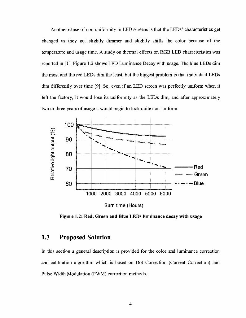
Another cause of non-uniformity in LED screens is that the LEDs' characteristics get
changed as they get slightly dimmer and slightly shifts the color because of the
temperature and usage time. A study on thermal effects on RGB LED characteristics was
reported in [1]. Figure 1.2 shows LED Luminance Decay with usage. The blue LEDs dim
the most and the red LEDs dim the least, but the biggest problem is that individual LEDs
dim differently over time [9]. So, even if an LED screen was perfectly uniform when it
left the factory, it would lose its uniformity as the LEDs dim, and after approximately
two to three years of usage it would begin to look quite non-uniform.
n a. -*—» o
D)
(1)
a:
100
90
80
70
60
• *•>*»
* •
z^^ma
•
"^B^5£S>
• ^
<sm%mi> ^
* ^ . ^
*«» e WSte
^ ^ • — Red
- —Green
Blue
1000 2000 3000 4000 5000 6000
Burn time (Hours)
Figure 1.2: Red, Green and Blue LEDs luminance decay with usage
1.3 Proposed Solution
In this section a general description is provided for the color and luminance correction
and calibration algorithm which is based on Dot Correction (Current Correction) and
Pulse Width Modulation (PWM) correction methods.
4

1. Dot Correction (Current correction)
The luminance of LEDs is determined by the amount of DC current that flows through
the P/N junction. More current produces a brighter LED. Unfortunately, however,
adjusting the current will also change the color of the LEDs.
Although, this method will reduce the color difference and can be used to make sure
that the modules all have the same luminance, but it cannot be used to correct the color
differences. Furthermore, if two modules were the same color before adjusting the current,
they would no longer be the same color after the adjustment.
2. Pulse Width Modulation (PWM) Correction
PWM is a widely used technique to control the luminance of LEDs [13]. It can be used to
process the video signal and also to perform color uniformity correction. PWM is used
instead of varying the current because changing the current of the LEDs would also
change the colors as explained above, while PWM does not change the LED color when
changing the brightness. PWM works by flashing the LEDs either fully on or fully off at
a very high rate. The flashes are so fast that the human eye cannot notice them and the
duration of the individual flashes (pulse width) determines the perceived luminance.
Video signal in a non-corrected system is turned into pulse widths by LED drivers to
flash the LEDs. In a corrected system, the pulse widths are multiplied by correction
coefficients before being sent to the LED drivers. Unfortunately, however, adjusting the
PWM will cut a lot of the LED output video resolution.
Our proposed solution is to use both methods in conjunction to achieve uniformed
color and Luminance LED screen with a high image resolution. In order to implement
these methods, a Robotic Spectrometer system was used to measure and adjust the
5

luminance and color of each displayed pixel.
The proposed methodology and algorithm were implemented and tested with
successful results.
1.4 Related Work
In this section the related work is presented in the area of color and luminance calibration
and correction systems for RGB LED pixels using various techniques and methodologies.
Also, different theoretical algorithms will be shown for color mixture and rendering.
Since LED video screens and LED lighting systems became more and more popular,
there is a need for an efficient and cost-effective design to fix the non-uniformity problem
in the color and luminance of the LED screens and modules as it is now competitive
requirement for LED screen manufacturers and owners who seek to deliver high image
quality and resolution. For instance, the offered solution in [11] proposes a color and
luminance correction and calibration using camera-based system. The camera uses
several optics and filters for measuring each color. The solution measures the LEDs'
colors and luminance data, then it analyses them using Windows based software. The
software calculates the correction coefficients and sends them back to the display to
perform the correction. The correction algorithm based on setting the current of the Red,
Green and Blue LEDs at certain values, and then it uses the PWM method to calibrate
and correct the LEDs colors and luminance. The correction algorithm is not published as
this is a commercial solution. As it was discussed before, this kind of solution is sensitive
to ambient temperature, light intensity, expensive and difficult to setup. The camera
6

needs a periodic calibration to be done by the manufacturer as it has different optics and
filters which are very hard to calibrate. Our proposed system uses an off-the-shelf
spectrometer and diffuser which can be calibrated by the user directly. In addition it is
easy to setup and run.
Another work has been presented in [28] for a robotic spectrometer system for LED
display measurements. It is a developed technique for measuring the luminosity and
operating characteristics of each LED in every pixel and stores them in a lookup table.
The aim of this technique is to allow the system to adjust the output luminance of each
LED based on the results of the lookup table. The provided technique is to be
incorporated as part of each display and to be hidden at the back of the display when not
in use, to facilitate periodic measurements in the field. This solution is not implemented
and it will increase the cost of each LED screen as it adds an extra complication to the
product. The proposed design in this thesis is to be implemented at the manufacturer
place and it calibrates both luminance and color non-uniformity in the LED pixels.
In [1] [2], the authors provide an overview of the white color accuracy required,
made of the red, green, and blue LEDs, in the general illumination market and the
challenges to achieve the required achromatic point (white light). It also shows how the
variation in lumen output and wavelength for nominally identical LEDs and the change in
these parameters with temperature and time result in an unacceptably high variability in
the color point of white light from RGB-LEDs. The work shows how they overcome
these problems using a feedback control schemes which can be implemented in a
practical LED lamp (or pixel). As for the work in [29], the authors provide color control
implementation using a laboratory setup based on a rapid color control prototyping
7

system which uses commercially available software and digital hardware amended by
custom in-house developed hardware. Both works base their color control on PWM
methodology. Our proposed technique bases its color and luminance control on both
PWM and Current amplitudes methodologies, which gives more resolution on the gray
level.
Several additive color mixing algorithms were introduced using the CIE color system.
In [27] the author shows a linear color mixing procedure which depends on the brightness
of the primary colors. It explains how adding two colors of light can be worked out as a
weighted average of the CIE chromaticity coordinates for the two colors. The weighting
factors involve the brightness parameters Y. This linear procedure is valid only if the
colors are relatively close to each other in value. In [31] the author shows color mixtures
procedures in CIE RGB and XYZ color spaces, in CIE xy Chromaticity Space, and in
CIE u V Chromaticity Space. The procedures depend on the primary colors weighting
factors. The weighting factors involve the brightness parameters. The procedures apply
the center of gravity law. Our proposed algorithm is a new linear color mixing algorithm
which depends only on calculating the weighting factors while the weighting factors are
independent of the primary colors' brightnesses. The algorithm is based on Grassmann's
laws of additive color mixture and it applies the center of gravity law.
1.5 Thesis Contribution
The contribution of this thesis is as follows:
• New correction and calibration algorithm and technique were developed to fit
LED video screens and LED lighting products and applications.
8
• Cost-effective, efficient, and simple solution was provided to solve the non-
uniformity of the color and luminance problem in LED screens.
• The resolution of the output video and the picture quality were improved for the
calibrated LED screens.
1.6 Thesis Outline
This thesis is made up of 6 chapters. Chapter 2 provides an overview of the light
definition and standards, where we introduce the CIE color spaces and definitions. In
addition, it provides an overview of the LED screen technology and architecture. In
Chapter 3, the color and luminance correction algorithm along with the developed
methodologies are presented. Chapter 4 presents the color and luminance correction and
calibration developed system and tools to implement the developed methodologies. In
Chapter 5, experimental results are presented. Conclusions and future work are presented
in chapter 6.
9
C H A P T E R 2
Pir@lnmnm&irii@s
2 d LEU) vMe© §cr©©nn§
Nowadays, LED video screens represent the most competitive large-scale display
technology. LED screen is like a giant television, but with one fundamental difference;
instead of the picture being beamed from a cathode ray tube, each pixel is made up of a
cluster of tiny LEDs. Each cluster has a red, green and blue LED, which light up
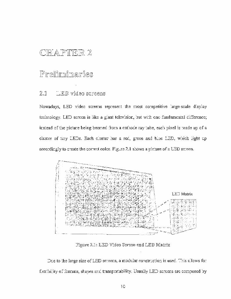
accordingly to create the correct color. Figure 2.1 shows a picture of a LED screen.
Fngwiire 2 At LEED Video Sereenn amndl LEED Mattrnx
Due to the large size of LED screens, a modular construction is used. This allows for
flexibility of formats, shapes and transportability. Usually LED screens are composed by
10
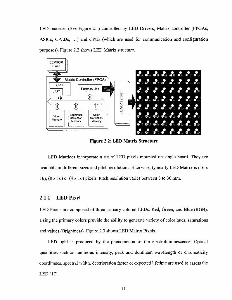
LED matrices (See Figure 2.1) controlled by LED Drivers, Matrix controller (FPGAs,
ASICs, CPLDs, ...) and CPUs (which are used for communication and configuration
purposes). Figure 2.2 shows LED Matrix structure.
Figure 2.2: LED Matrix Structure
LED Matrices incorporate a set of LED pixels mounted on single board. They are
available in different sizes and pitch resolutions. Size wise, typically LED Matrix is (16 x
16), (8 x 16) or (4 x 16) pixels. Pitch resolution varies between 3 to 30 mm.
2.1.1 LED Pixel
LED Pixels are composed of three primary colored LEDs: Red, Green, and Blue (RGB).
Using the primary colors provide the ability to generate variety of color hues, saturations
and values (Brightness). Figure 2.3 shows LED Matrix Pixels.
LED light is produced by the phenomenon of the electroluminescence. Optical
quantities such as luminous intensity, peak and dominant wavelength or chromaticity
coordinates, spectral width, deterioration factor or expected lifetime are used to assess the
LED [17].
11

Figure 2.3: LED Matrix Pixel
2.1.2 Properties of LEDs
Optical prosperities of LEDs:
The radiation of a LED can be characterized by radiometric and spectroradiometric
quantities. Visible light LED also requires photometric and colorimetric quantities to
quantify its effect on the human eye. Consequently, radiometric, spectroradiometric,
photometric and colorimetric quantities with their related units may all have to be used to
characterize the optical radiation emitted by LED [15]. For the proposed algorithm in this
thesis, Colorimetric quantities such as; luminosity (which represents the LED brightness)
and chromaticity coordinates (which represents the LED color), were the only needed
quantities to measure and calibrate the non-uniformity problems in the LEDs.
Colorimetric quantities are determined from the LED spectral power distribution (SPD).
Typical single-color LEDs have quasi-monochromatic spectral distribution, with
spectral bandwidth that are typically a few 10 nanometers wide, which is something
between monochromatic spectral distribution (as emitted by laser) and broad-band
spectral distribution (as found with white LED) [15]. Figure 2.4 shows the three different
spectral distribution types.
12

400 450 650 700 500 550 600
Wavelengths (nm)
Figure 2.4: (a) Broad-band spectral, (b) monochromatic, (c) quasi-monochromatic.
The proposed technique in this thesis uses CCD-based Spectrometer to measure the
LEDs spectral power distribution. As reported in [15], the spectral distribution can be
measured with a spectrometer in four different methods: 1) irradiance mode, 2) total flux
mode, 3) partial flux mode and 4) radiance mode. In irradiance mode, the spectral
distribution of a LED is measured in one direction, whereas, in total flux mode, they are
measured as an average of all directions. The partial flux mode is in between. The
radiance mode measures the spectral radiance of the LED surface, using an imaging optic
with the photometer.
Fiber
Diffuser
W&iV//
Figure 2.5: Irradiance Mode
13
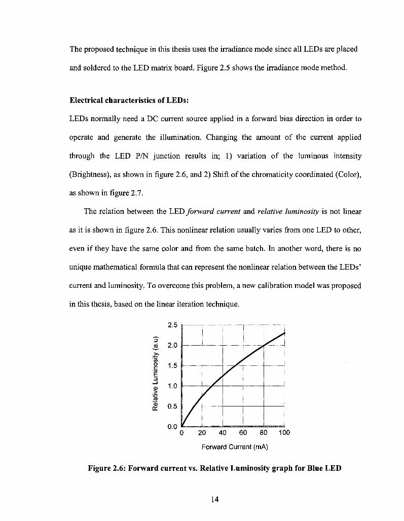
The proposed technique in this thesis uses the irradiance mode since all LEDs are placed
and soldered to the LED matrix board. Figure 2.5 shows the irradiance mode method.
Electrical characteristics of LEDs:
LEDs normally need a DC current source applied in a forward bias direction in order to
operate and generate the illumination. Changing the amount of the current applied
through the LED P/N junction results in; 1) variation of the luminous intensity
(Brightness), as shown in figure 2.6, and 2) Shift of the chromaticity coordinated (Color),
as shown in figure 2.7.
The relation between the LED forward current and relative luminosity is not linear
as it is shown in figure 2.6. This nonlinear relation usually varies from one LED to other,
even if they have the same color and from the same batch. In another word, there is no
unique mathematical formula that can represent the nonlinear relation between the LEDs'
current and luminosity. To overcome this problem, a new calibration model was proposed
in this thesis, based on the linear iteration technique.
2.5
1 2.0
g 1.5 '£
>
& 0.5
0.0 0 20 40 60 80 100
Forward Current (mA)
Figure 2.6: Forward current vs. Relative Luminosity graph for Blue LED
14
0.06 0.1 0.11 0.12 0.13 0.14 0.15
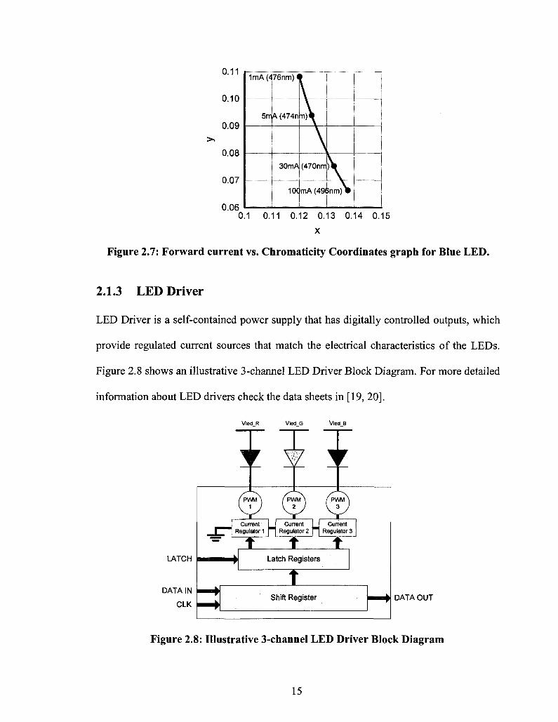
X
Figure 2.7: Forward current vs. Chromaticity Coordinates graph for Blue LED.
2.1.3 LED Driver
LED Driver is a self-contained power supply that has digitally controlled outputs, which
provide regulated current sources that match the electrical characteristics of the LEDs.
Figure 2.8 shows an illustrative 3-channel LED Driver Block Diagram. For more detailed
information about LED drivers check the data sheets in [19, 20].
Vied R Vled_G Vied B
LATCH
DATA IN
CLK Shift Register DATA OUT
Figure 2.8: Illustrative 3-channel LED Driver Block Diagram
15
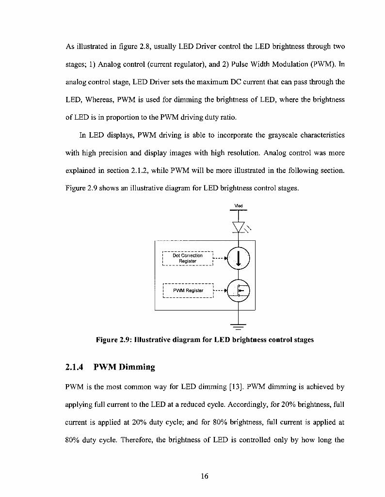
As illustrated in figure 2.8, usually LED Driver control the LED brightness through two
stages; 1) Analog control (current regulator), and 2) Pulse Width Modulation (PWM). In
analog control stage, LED Driver sets the maximum DC current that can pass through the
LED, Whereas, PWM is used for dimming the brightness of LED, where the brightness
of LED is in proportion to the PWM driving duty ratio.
In LED displays, PWM driving is able to incorporate the grayscale characteristics
with high precision and display images with high resolution. Analog control was more
explained in section 2.1.2, while PWM will be more illustrated in the following section.
Figure 2.9 shows an illustrative diagram for LED brightness control stages.
Vied
r , S - X i Dot Correction ] J. I \ i Register i " v • • I -:- I i 1 V * > /
i PWM Register • • - - - • [ • • * - ' . )
Figure 2.9: Illustrative diagram for LED brightness control stages
2.1.4 PWM Dimming
PWM is the most common way for LED dimming [13]. PWM dimming is achieved by
applying full current to the LED at a reduced cycle. Accordingly, for 20% brightness, full
current is applied at 20% duty cycle; and for 80% brightness, full current is applied at
80% duty cycle. Therefore, the brightness of LED is controlled only by how long the
16
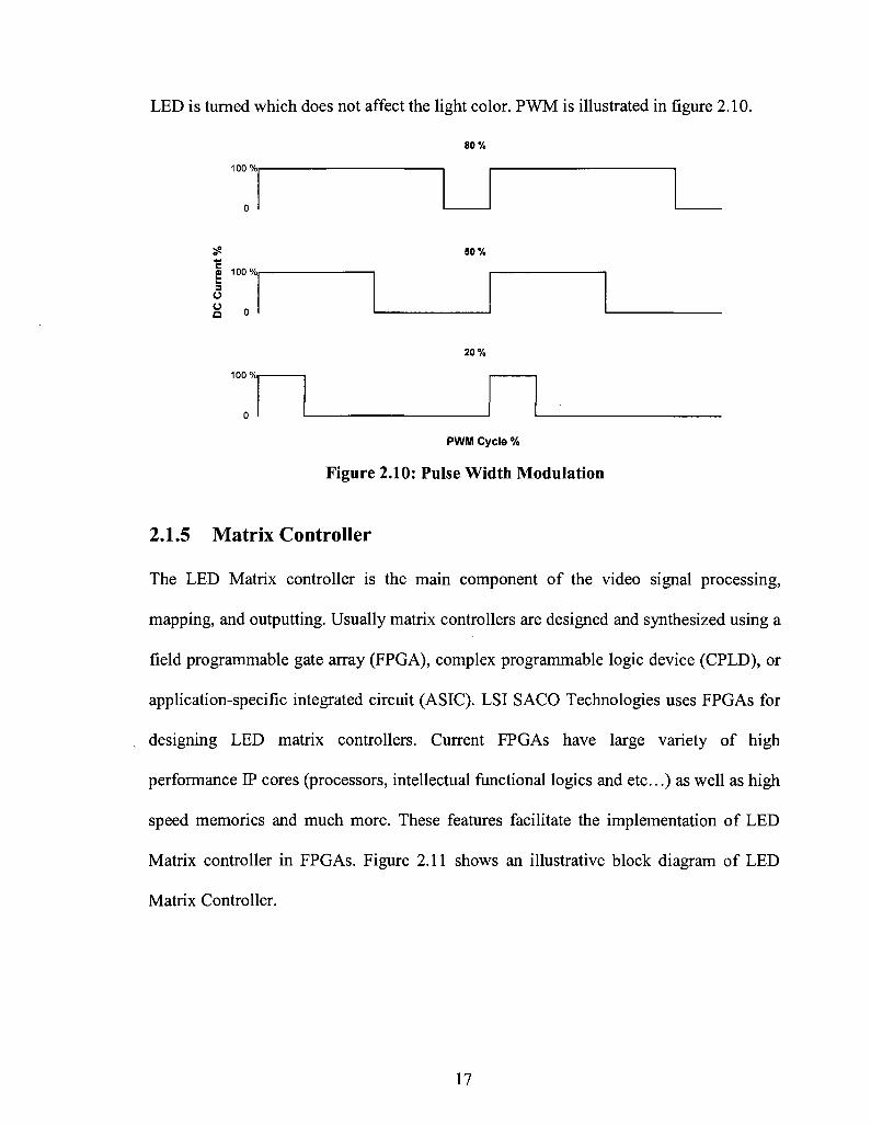
LED is turned which does not affect the light color. PWM is illustrated in figure 2.10.
80%
100 %| 1 | 1
o I 1
3? 50 %
S 100%i 1 1 1
3
o
8 o I 1 I 20%
100 %| 1 I 1
o I 1 I
PWM Cycle %
Figure 2.10: Pulse Width Modulation
2.1.5 Matrix Controller
The LED Matrix controller is the main component of the video signal processing,
mapping, and outputting. Usually matrix controllers are designed and synthesized using a
field programmable gate array (FPGA), complex programmable logic device (CPLD), or
application-specific integrated circuit (ASIC). LSI SACO Technologies uses FPGAs for
designing LED matrix controllers. Current FPGAs have large variety of high
performance IP cores (processors, intellectual functional logics and etc..) as well as high
speed memories and much more. These features facilitate the implementation of LED
Matrix controller in FPGAs. Figure 2.11 shows an illustrative block diagram of LED
Matrix Controller.
17

Communication Link
CLK
Video IN
EEPROM Flash
\ A -\1
^ M Matrix Controller (FPGA)
CPU
UART Process Unit
£ 4 I
Video Memory
Brightness Correction Memory
I Color
Correction Memory
To LED Drivers
Figure 2.11: Illustrative block diagram of LED matrix controller
EEPROM Flash: is used to store the FPGA binary file, the matrix configuration data,
and the correction coefficients data. The FPGA binary file is an encoded data file which
contains the raw bits that need to be stored inside the FPGA to program the chip. The
Matrix configuration data contain information about the size of the matrix, the video
memory mapping, and other more matrix details. The correction coefficients data are
used to correct the LED pixels brightness and color data (Usually. They are set to default
values when the LED matrix is not calibrated). In the next chapter, the matrix calibration
process will be explained more in details along with how to assign the coefficients values.
CPU: is the main microcontroller unit that controls all the communication links
between the FPGA, EEPROM Flash, and the external systems to the LED Matrix. The
CPU loads, from the EEPROM, the stored matrix configuration data to the FPGA, and it
loads the correction coefficients and values to the brightness correction memory and the
color correction memory. CPU uses Universal Asynchronous Receiver/Transmitter
(UART) interface to communicate with the external systems, and Serial Peripheral
18
Interface (SPI) bus to communicate with the EEPROM flash.
Process Unit: is the main component inside the matrix controller where all the data
calculations are performed. It grabs all the pixels data from the memories, processes them,
calculates the brightness and color of each LED, builds the data string, and then sends
them to the LED Driver. In the next chapter, the calculation process of the LED color and
brightness data will be explained more in details.
2.2 Light and Color
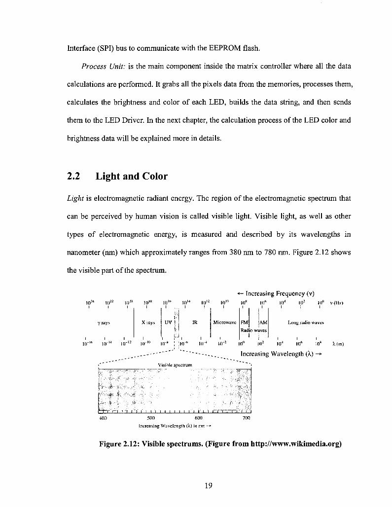
Light is electromagnetic radiant energy. The region of the electromagnetic spectrum that
can be perceived by human vision is called visible light. Visible light, as well as other
types of electromagnetic energy, is measured and described by its wavelengths in
nanometer (nm) which approximately ranges from 380 nm to 780 ran. Figure 2.12 shows
the visible part of the spectrum.
Increasing Frequency (v) IOM SO22 IO20 10 , s 10"' IO14 IO12 K)10 10* 10s 104 Ifl2 10° v(Hz)
I l ) . > . I „ „ l I . I . I . . I . I I I
y rays X rays UV IR
- ' < • ,0-H io-'2 l0-ID i
io~* D 1 1
10
Microwave-
10"'
FM AM
Radio waves 1 1 10"
Long radio waves
IO2 I0J 10* IO8 X(m)
Increasing Wavelength (k) -*
Visible spectrum
-*TTrTrTrJ-r-rJT-THrT~i-~i < i i i i i' Tn r~m-nr i~-TT^nr"r~ ,r '-400 500 600 700
Increasing Wavelength (X) in nm -»
Figure 2.12: Visible spectrums. (Figure from http://www.wikimedia.org)
19
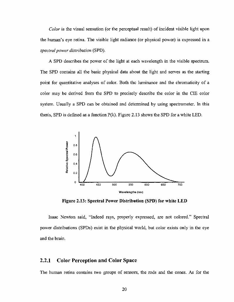
Color is the visual sensation (or the perceptual result) of incident visible light upon
the human's eye retina. The visible light radiance (or physical power) is expressed in a
spectral power distribution (SPD).
A SPD describes the power of the light at each wavelength in the visible spectrum.
The SPD contains all the basic physical data about the light and serves as the starting
point for quantitative analyses of color. Both the luminance and the chromaticity of a
color may be derived from the SPD to precisely describe the color in the CEE color
system. Usually a SPD can be obtained and determined by using spectrometer. In this
thesis, SPD is defined as a function P(X-). Figure 2.13 shows the SPD for a white LED.
1
I 0.8 o Q.
15 t j 0.6 a a. W 5 0.4 12 a * 0.2
0 400 450 500 550 600 650 700
Wavelengths (nm)
Figure 2.13: Spectral Power Distribution (SPD) for white LED
Isaac Newton said, "Indeed rays, properly expressed, are not colored." Spectral
power distributions (SPDs) exist in the physical world, but color exists only in the eye
and the brain.
2.2.1 Color Perception and Color Space
The human retina contains two groups of sensors, the rods and the cones. As for the
20

cones, it has three types of color photoreceptor cone cells, which respond to incident
radiation with different spectral response curves. On the other hand, rods are effective
only at extremely low light intensities. The signals from these color sensitive cells
(cones), together with those from the rods, are combined in the brain to give several
different "sensations" of the color.
As humans, we may define these sensations in term of its attributes of brightness,
Hue, colorfulness, lightness, chroma, and saturation which have been defined by the
Commission Internationale de L'Eclairage (CIE) [22] and Hunt's book "Measuring
Colour" [21] as follows:
• Brightness: "the attribute of a visual sensation according to which an area appears
to emit more or less light" [22].
• Hue: "the attribute of a visual sensation according to which an area appears to be
similar to one of the perceived colors, red, yellow, green and blue, or a
combination of two of them" [22].
• Colorfulness: "the human sensation according to which an area appears to exhibit
more or less of its hue" [21].
• Lightness: "the sensation of an area's brightness relative to a reference white in
the scene" [21].
• Chroma: "the colorfulness of an area relative to the brightness of a reference
white" [21].
• Saturation: "the colorfulness of an area judged in proportion to its brightness"
[22].
On the other hand, color systems (or models) interpret these sensations using color
21
space which is a method by which they can specify, create and visualize color. The CIE
has defined a color system that classifies any colored light in the visible spectrum
according to the visual sensations mentioned above. A color is thus usually specified
using three co-ordinates, or parameters. These parameters describe the position of the
color within the color space being used. They do not tell us what the color is, that
depends on what color space is being used.
2.3 CIE Color system
The International Commission on Illumination - also known as the CIE from its French
title, the Commission Internationale de l'Eclairage - is an international organization,
located in Vienna, which worked in the first half of the 20th century developing a method
for systematically measuring color in relation to the wavelengths they contain. This
system became known as the CIE color system (or model). The model was originally
developed based on the trichromatic theory of color perception. The theory describes the
way three separate lights, red, green and blue, can match any visible color - based on the
fact of the eye's use of three different types of color sensitive photoreceptors cells (cones)
as was explained in section 2.2. These three photoreceptors respond differently to
different wavelengths of visible light.
The CIE had measured this differential response of the three cones in the eye, by
matching spectral colors to specific mixtures of the three colored lights, to define the CIE
color matching functions x{X), y(A) and z(A).
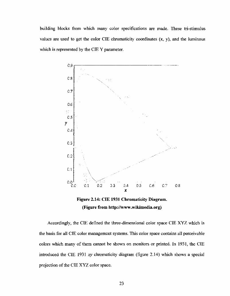
The SPD of a color is cascaded with these matching functions, over the visual range
from 380 to 780 nm, to produce three CIE tri-stimulus values X, Y, and Z, which are the
22
y 0.4
building blocks from which many color specifications are made. These tri-stimulus
values are used to get the color CIE chromaticity coordinates (x, y), and the luminous
which is represented by the CIE Y parameter.
0,9
0.8
0.7
0.6
0.2
0.1
0.0 0,0 0.1 0,2 0,3 QA 0.5 0.6 0.7
X
Figure 2.14: CIE 1931 Chromaticity Diagram.
(Figure from http://www.wikimedia.org)
0,8
Accordingly, the CIE defined the three-dimensional color space CIE XYZ which is
the basis for all CIE color management systems. This color space contains all perceivable
colors which many of them cannot be shown on monitors or printed. In 1931, the CIE
introduced the CIE 1931 xy chromaticity diagram (figure 2.14) which shows a special
projection of the CIE XYZ color space.
23
2.3.1 CIE color matching functions
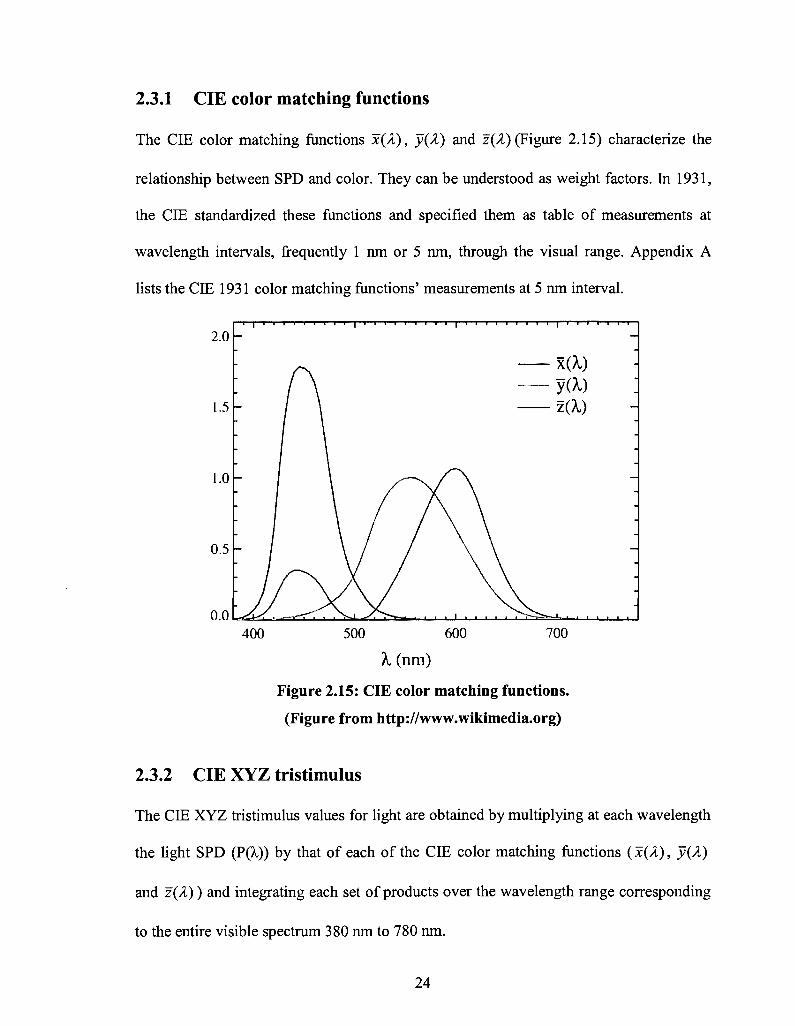
The CIE color matching functions x(A,), y(X) and z{X) (Figure 2.15) characterize the
relationship between SPD and color. They can be understood as weight factors. In 1931,
the CIE standardized these functions and specified them as table of measurements at
wavelength intervals, frequently 1 nm or 5 ran, through the visual range. Appendix A
lists the CIE 1931 color matching functions' measurements at 5 nm interval.
2.0
1.5
1.0
0.5
0.0 400 500 600 700
X (nm)
Figure 2.15: CIE color matching functions.
(Figure from http://www.wikimedia.org)
2.3.2 CIE XYZ tristimulus
The CIE XYZ tristimulus values for light are obtained by multiplying at each wavelength
the light SPD (P(X,)) by that of each of the CIE color matching functions (x(A), y{X)
and z{X)) and integrating each set of products over the wavelength range corresponding
to the entire visible spectrum 380 nm to 780 nm.
24
780
X= \x(A)P{X)dX 2.1(a) 380
780
Y= \y{X)P{X)dX 2.1(b) 380
780
Z = \z(X)P{X)dX 2.1(c) 380
The integration may be carried out by numerical summation at wavelength intervals,
AX, equal to 1 nm, 5 nm, or 10 nm.
780
X = AA^x(A)P(A) 2.2(a) /t=380
780
Y = AAY,y(VP(V 2.2(b) /t=380
780
Z = AA^z(A)PW 2.2(c) /t=380
The CIE Y value represents the luminance of the measured light source. Due to the
nonlinearities in the human visual system, this measurement is roughly correlated, with
but not equal to, the perceived brightness of the light source. In color and brightness
correction, we are usually interested only in relative luminosities so we can ignore
absolute values of Y and simply scale luminosities between user-defined minimum and
maximum brightnesses.
2.3.3 CIE 1931 chromaticity coordinates
The CIE 1931 chromaticity coordinates (x,y,z) are calculated from the tristimulus
values X, Y and Z as follows:
25
X X~ X + Y + Z
Y y =
X + Y + Z
Z Z~ X + Y + Z
The third coordinate, is redundant since,
x + y + z = l=>z = l-x-y
Therefore, it is sufficient to quote (x, y) only.
2.3.4 CIE1976wV
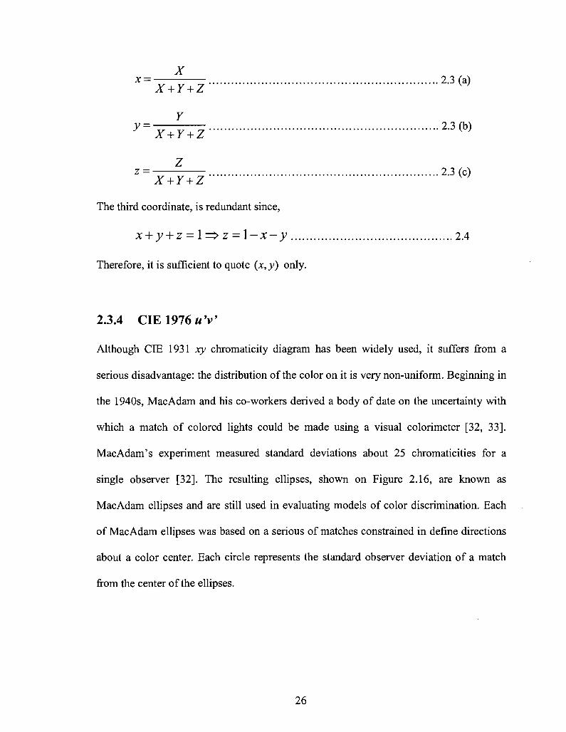
Although CIE 1931 xy chromaticity diagram has been widely used, it suffers from a
serious disadvantage: the distribution of the color on it is very non-uniform. Beginning in
the 1940s, MacAdam and his co-workers derived a body of date on the uncertainty with
which a match of colored lights could be made using a visual colorimeter [32, 33].
MacAdam's experiment measured standard deviations about 25 chromaticities for a
single observer [32]. The resulting ellipses, shown on Figure 2.16, are known as
MacAdam ellipses and are still used in evaluating models of color discrimination. Each
of MacAdam ellipses was based on a serious of matches constrained in define directions
about a color center. Each circle represents the standard observer deviation of a match
from the center of the ellipses.
2.3 (a)
2.3 (b)
2.3 (c)
. . . .2.4
26
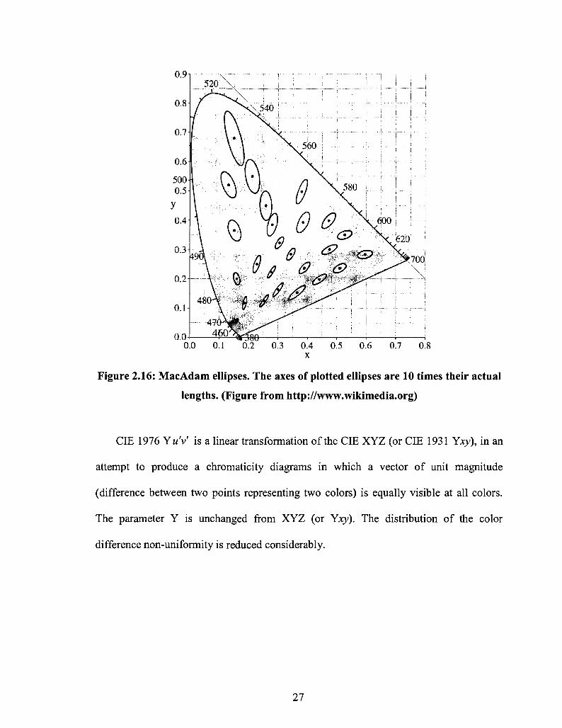
Figure 2.16: MacAdam ellipses. The axes of plotted ellipses are 10 times their actual
lengths. (Figure from http://www.wikimedia.org)
CIE 1976 Yu'V is a linear transformation of the CIE XYZ (or CIE 1931 Yxy), in an
attempt to produce a chromaticity diagrams in which a vector of unit magnitude
(difference between two points representing two colors) is equally visible at all colors.
The parameter Y is unchanged from XYZ (or Yxy). The distribution of the color
difference non-uniformity is reduced considerably.
27
Oti
S19
S» 0.S
0.4
0 3
V'
0.2
0.1
no »
,
'
a : \
v
480
540 no
- - - L - _ .
A
\ \ \ \
470
560 IWU
i
\ m
«o 440
438
560 590
/ /
/
an
/ / /
/
619
/ /
610
/ /
« 640
" " - - - • —
/ /
0.2 » u , 03 0.5 0.6
Figure 2.17:1976 CIE « V chromaticity diagram.
(Figure from http://www.wikimedia.org)
The chromaticity diagram shown in Figure 2.17 is known as CIE 1976 uniform
chromaticity diagram or CIE 1976 UCS diagram, commonly referred to as CIE wV
chromaticity diagram. It is obtained as:
4x u =•
v =
•2x + l2y + 3
2JC + 12J> + 3
2.5(a)
2.5(b)
The CIE u'v diagram is useful for showing the relationships between colors
whenever the interest lays in their discriminability. Both chromaticity diagrams, CIE xy
and CIE u'v', have the property that additive mixture of colors are represented by points
lying on the straight line joining the points representing the constituent colors.
28
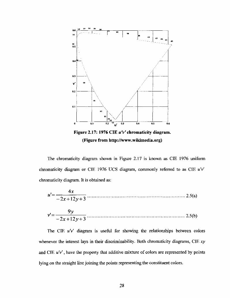
2.4 Color Gamut
A color gamut is the set of possible colors a device can reproduce within a color space.
The color chromaticity and the brightness of the primary colors (the red, the green and
the blue) determine the color gamut of the device.
Y
0.8
0.6
0.3
0.1
Adobe RGB
• 3 i /
NTSC
•LED
4CCFL
0.1 0.2 0.3 0.4 0.5 0.6 0.7
Figure 2.18: Color Gamuts. It shows the color gamut for: Adobe RGB, NTSC
(National Television System Committee), CCFL (Cold cathode fluorescent lamps),
and LEDs in general. (Picture from http://www.nec-lcd.com)
Often the gamut will be represented in only two dimensions, for example on a CIE
xy chromaticity diagram. Figure 2.18 shows an example of the color gamut for different
systems.
29

2.5 Additive Color Mixture
2.5.1 Grassmann's Laws of additive color mixture
In 1953 the German mathematician Hermann Giinther Grassmann discovered and
introduced laws concerned with the results of mixing colored lights. Simple explanation
for the laws was illustrated in [26], "Any color (source C) can be matched by a linear
combination of three other colors (primaries e.g. RGB), provided that none of those three
can be matched by a combination of the other two. This is fundamental to colorimetry
and Grassman's first law of color mixture. So a color C can be matched by Re units of
red, Gc units of green and Be units of blue. The units can be measured in any form that
quantifies light power.
C = Re (R) + Gc (G) + Be (B) 2.6
A mixture of any two colors (sources CI and C2) can be matched by linearly adding
together the mixtures of any three other colors that individually match the two source
colors. This is Grassman's second law of color mixture. It can be extended to any number
of source colors.
C3(C3) = CI (CI) + C2(C2) = [Rl + R2](R) + [Gl + G2](G) + [Bl + B2](B)...2.1
Color matching persists at all luminances. This is Grassman's third law. It fails at
very low light levels where rod cell vision (scoptopic) takes over from cone cell vision
(photopic).
kC3[C3] = kClfCl] + kC2[C2] 2.8
The symbols in square brackets are the names of the colors, and not numerical values.
The equality sign should not be used to signify an identity; in colorimetry it means a
30
color matching, the color on one side of the equality looks the same as the color on the
other side.
These laws govern all aspects of additive color work, but they apply only signals in
the "linear-light" domain. They can be extended into subtractive color work."
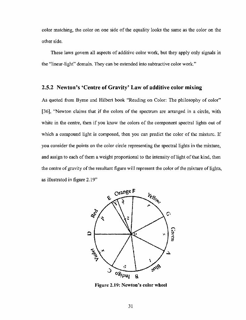
2.5.2 Newton's 'Centre of Gravity' Law of additive color mixing
As quoted from Byrne and Hilbert book "Reading on Color: The philosophy of color"
[36], "Newton claims that if the colors of the spectrum are arranged in a circle, with
white in the centre, then if you know the colors of the component spectral lights out of
which a compound light is composed, then you can predict the color of the mixture. If
you consider the points on the color circle representing the spectral lights in the mixture,
and assign to each of them a weight proportional to the intensity of light of that kind, then
the centre of gravity of the resultant figure will represent the color of the mixture of lights,
as illustrated in figure 2.19"
Figure 2.19: Newton's color wheel
31
"Newton's color wheel (Figure 2.19): to predict the color of mixtures of light. The
circumference DEFGABCD represents "the whole Series of Colors from one end of the
Sun's colored Image to the other." Let/?, q, r, s, t, v, x be the "Centers of Gravity of the
Arches" DE, EF, FG, GA, AB, BC and CD, respectively; "and about those Centers of
Gravity let Circles proportional to the Number of Rays of each Color in the given
Mixture be described." "Find the common Center of Gravity of all those Circles, p, q, r, s,
t, v, x. Let that Center be Z; and from the Center of the Circle ADF, through Z to the
Circumference, drawing the Right Line OY, the place of the Point Y in the Circumference
shall show the Color arising from the Composition of all the Colors in the given
Mixture." The ratio of OZ to the radius of the circle gives the relative saturation of the
color. (From Newton, Opticks, 154-5.)".
2.5.3 Additive Color Mixing with CIE
The result of adding two colors of light can be worked out as a weighted average of the
CIE chromaticity coordinates for two colors [27]. The weighting factors involve the
brightness parameters Y. If the coordinates of the two colors are;
xj, yi with brightness Yi X2, y2 with brightness Y2
then the additive mixture color coordinates are;
Y\ Yi Y\ Yi X3 = X\-\ X2 V3 = Vl H V2 2 9
Y1 + Y2 Y1 + Y2 ' Y1 + Y2 Y\ + Y2
"This linear procedure is valid only if YI and Y2 are reasonably close to each other
in value". "They say that each of the resulting chromaticity coordinates (say, x3) is the
average of the respective coordinates of the components (xl and x2) weighted according
32

to their relative contributions to the total luminance. This is sometimes called the "Center
of Gravity"" Quoted from [27].
2.6 PWM Correction Methodology
Pulse Width Modulation (PWM) is mainly used for light dimming as was explained in
section 2.1.4. In this section, another use for the PWM will be explained as a correction
methodology for LED lighting products.
PWM correction has proven to be the best method for correcting uniformity
problems in LED screens and LED lighting systems. The methodology works by
modifying the pulse widths for each pixel to compensate for the brightness variations of
LEDs. By adjusting the brightness of the individual LEDs in an LED screen pixel, the
color of the LED pixel can be selectively adjusted to a target color. In an uncorrected
LED screen, the video signal is turned directly into pulse widths by the LED drivers to
flash the LEDs. In a corrected system, the video signal is multiplied by correction
coefficients by the LED matrix controller before it is sent to the LED drivers. The
correction coefficients are computed for every color in the LED pixel in such a way as to
correct the luminance and the color coordinates. The computation process will be
explained in chapter 3.
The PWM correction methodology is applied to each color LED in each pixel in the
LED screen. The concept behind the correction methodology is to light up the three
tristimulus colors (RGB) with a certain amounts to create the target color. To illustrate
the methodology further more, the following example is given;
33
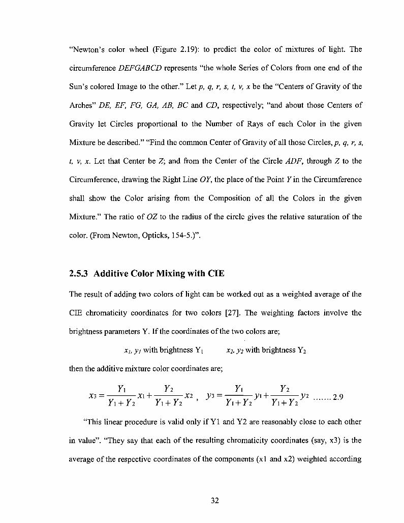
Example 2.1:
Assume that we have LED pixel with the following RGB color and luminance;
Yr = 110 nits, u' r= 0.52, v \ = 0.54
Yg = 200 nits, u'g= 0.09, v'g = 0.58
Yb = 60 nits, u'b = 0.15, v'b = 0.21
And we wish to correct the red color to the following target color and luminance;
Target luminance: 105 nits
Target color coordinates: u'r_t= 0.49, v'r_t= 0.51
The system will compute the red, green and blue coefficients which needed to correct the
red according to the target color and luminance;
Let's assume for R = 90% the G = 1.5%, and the B = 5%
Total Brightness = (0.9 x 110) + (0.015 x 200) + (0.05 x 60) = 105 nits
Accordingly, the red signal was reduced by a factor of 0.9 and some green and blue was
added to achieve the desired targets. Figure 2.20 shows the red coefficients before and
after the correction.
RED Correction Coefficients (No Correction) --- -
Video Signal Out
Figure 2.20: Red coefficients before and after correction
34
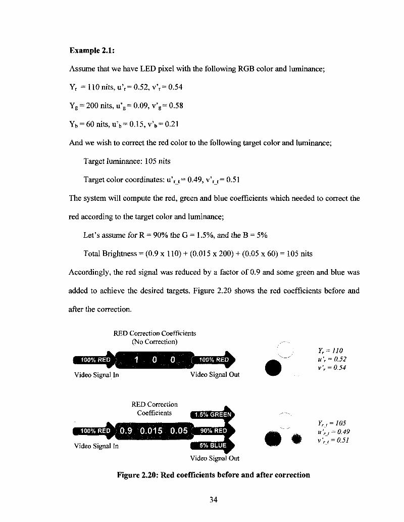
The previous example just showed the sequence to correct one color in one pixel of
the LED screen. To correct the complete LED screen, this process must be applied to
each color (Red, Green, and Blue) for each pixel in the LED screen. Therefore, the final
correction coefficients will be a 3x3 matrix for each pixel as shown in figure 2.21 below.
The Coefficients will be stored in the LED matrix controller where they will be
multiplied by the video signal stream when video is being displayed on the screen.
FULL LED Pixel Correction Coefficients
Figure 2.21: Full LED pixel correction coefficients
35

CHAPTER 3
Correction and Calibration Algorithms
3.1 Introduction
In this Chapter, the color and luminance correction and calibration algorithms will be
presented. The Correction algorithm deals mainly with the color non-uniformity problem
of the LED pixels, while the Calibration deals with their luminance variation problem.
The algorithms are based on the Current and PWM correction methods where they use
the CIE color systems to measure, calibrate, and correct the LEDs colors and Luminances.
3.2 Luminance Calibration Algorithm
The proposed luminance calibration algorithm and process is based on the Dot
Correction (Current Correction) methodology based on controlling the current passing
through each LED in each pixel individually. Since the relation between the LED
forward current and relative luminosity is not linear, as was discussed in section 2.1.2,
the calibration process is implemented based on the linear iteration technique.
The proposed algorithm has two inputs and one output. The inputs are represented by
the default current value (Cdefuait) and the target luminance (Ytarget) for the LED, while the
output is represented by the target current (Garget)- The algorithm consists of two main
steps which will be explained in the following calibration process for red LED in a target
36
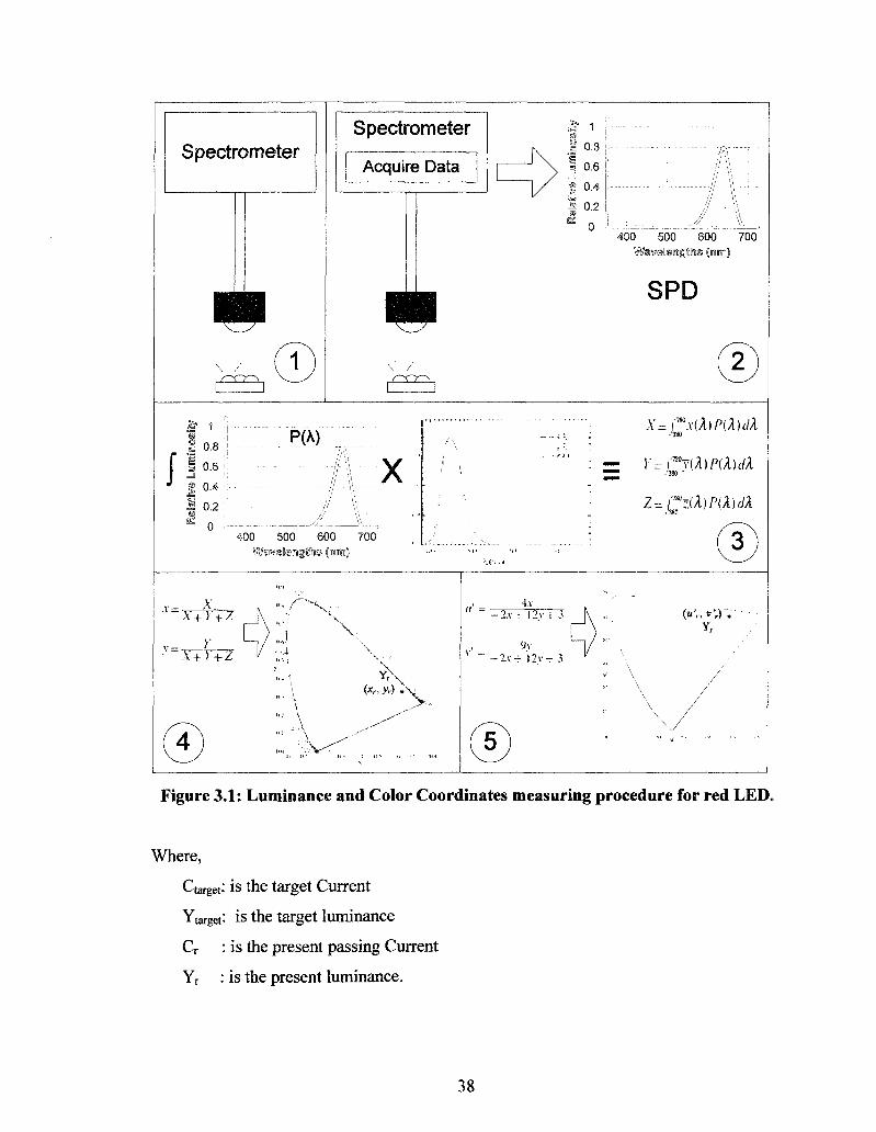
pixel. The green and blue LEDs luminance calibration process is identical to the red LED
calibration process.
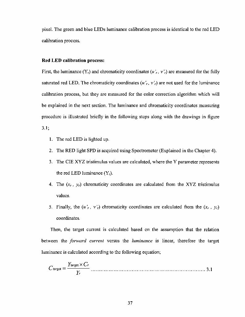
Red LED calibration process:
First, the luminance (Yr) and chromaticity coordinates (u'r, vV) are measured for the fully
saturated red LED. The chromaticity coordinates (u 'r, v'r) are not used for the luminance
calibration process, but they are measured for the color correction algorithm which will
be explained in the next section. The luminance and chromaticity coordinates measuring
procedure is illustrated briefly in the following steps along with the drawings in figure
3.1;
1. The red LED is lighted up.
2. The RED light SPD is acquired using Spectrometer (Explained in the Chapter 4).
3. The CIE XYZ tristimulus values are calculated, where the Y parameter represents
the red LED luminance (Yr).
4. The (xr, yr) chromaticity coordinates are calculated from the XYZ tristimulus
values.
5. Finally, the (u'r, v'r) chromaticity coordinates are calculated from the (xr, yr)
coordinates.
Then, the target current is calculated based on the assumption that the relation
between the forward current versus the luminance is linear, therefore the target
luminance is calculated according to the following equation;
_ /target X t r Ctarget = 3.1
37
Spectrometer Spectrometer
Acquire Data
^ « H i
.1 °-8
I 0.6
| 0 2
K 0 W 500 600 700
SPD
J 1 ;i
0.8 |
0.6 ;•
0.4
0.2
PW
X
400 500 600 700 Waweleoigftte (mm)
.380
y=rv(A)P(A)t/A • •380 • '
Z = / , 8 0 ; ( A ) / > ( A M A
A'+r+z
Y X+Y+Z
©
V
(x„yr) ^ V
4.v -2.V • 12.V : 3
"~2v'-r 12v"^ 3
Yr
© Figure 3.1: Luminance and Color Coordinates measuring procedure for red LED.
Where,
Ctarget: is the target Current
Ytarget is the target luminance
Cr : is the present passing Current
Yr : is the present luminance.
38

Since the luminance-current relation is not linear, the algorithm uses the iteration
technique to achieve the target luminance. The iteration technique runs the two steps
mentioned above (The Luminance and Color Coordinates measuring, and Target current
calculation) at every iteration turn. The following example will illustrate and explain the
iteration process;
Example: Assume that the Target Luminance (Ytarget) for a LED is 60, the present Current
(Ci) is 1, and the Current vs. Luminosity curve as shown in figure 3.2.
100
0.0 0.2 0.4 0.6 0.8 1
Forward Current
Figure 3.2: Current vs. Luminosity (Example)
To achieve the target luminance, the algorithm will go through the following steps:
1. It lights the LED with the default current (Ci) and Measures the current
luminance (Yi). It uses the point (Ci, Yi) and (Co, Yo) to create the assumed linear
relation line between the current and luminance (Figure 3.3).
39

100
80
CO
o c F 3
60
40
' t irgeL^
s s
I /
(Ci , Y r
20
0 A^b 0.2 0.4 0.6 0.8 1
£° Forward Current
Figure 3.3: Light and measure (Ci, Yi)
2. It calculates the new current value (C2) using equation 3.1, and uploads it to the
LED in order to measure the new luminance (Y2) (Figure 3.4).
100
80
CO
0 c F D
60
40
20
1
\
Yt
9 /
n , — ¥ , 1 J
"J>?M • 7 * f '
1
s s
s
'
s (Ci , Y,)
£* A^0 0.2 0.4 0.6 0.8 1
Forward Current
Figure 3.4: Light and measure (C2, Y2)
3. Since (Y2 > Ytarget), it uses the point (C2, Y2) and (Co, Yo) to create the new linear
line. Then it calculates the new current (C3) and uploads it to the LED to measure
the new luminance (Y3) (Figure 3.5).
40

100
80
8 60 c
u 40
20
0
/
<(' \*'
/ / / /
-, Y-. i 7 k"
i # ' larj et , f(c3 , y,)
' '
? * -
£° A O 0.2 0.4 0.6 0.8 1
Forward Current
Figure 3.5: Light and measure (C3, Y3)
4. Since (Y3 < Ytarget), it uses the point (C2, Y2) and (C3, Y3) to create the linear line.
Then it calculates the new current and uploads it to the LED to measure the new
luminance. If the new luminance equals to the target luminance (Ytarget) then the new
current will represent the target current (Ctarget) (Figure 3.6).
100
0.0 0.2 0.4 0.6 0.8 1
Forward Current
Figure 3.6: Light and measure (Ctarget) Ytarget)
Figure 3.7 shows the luminance calibration algorithm flowchart.
41
Start
I Light LED
Upload (Cnew) to LED
Calculate new current value
V^newJ
Figure 3.7: Luminance calibration process flowchart
The same procedure is done for the green and the blue LEDs to have at the end of the
process the luminance and color for each LED in the pixel (Figure 3.8).
w//
Spectrometer Spectiometer
w//
Yr (U'r, V'r) Y g (u'g , V'g) Y b (u'b , V'b)
Figure 3.8: RGB LEDs luminance and color values
42

3.3 Color Correction Algorithm
The purpose of the color correction algorithm, as was discussed in chapter 1, is to solve
the color non-uniformity problem in the LED screen's pixels. To achieve this purpose,
the color correction algorithm shifts every color in each individual pixel to one target
chromaticity coordinates. Therefore, all measured greens' chromaticity coordinates will
be shifted to one target green chromaticity coordinate (GtargetX measured reds to a target
red (Rtarget), and measured blues to a target blue (Btarget)- The target white (Wtarget) will be
achieved by determining the right luminance values for the target colors (Rtarget, Gtarget,
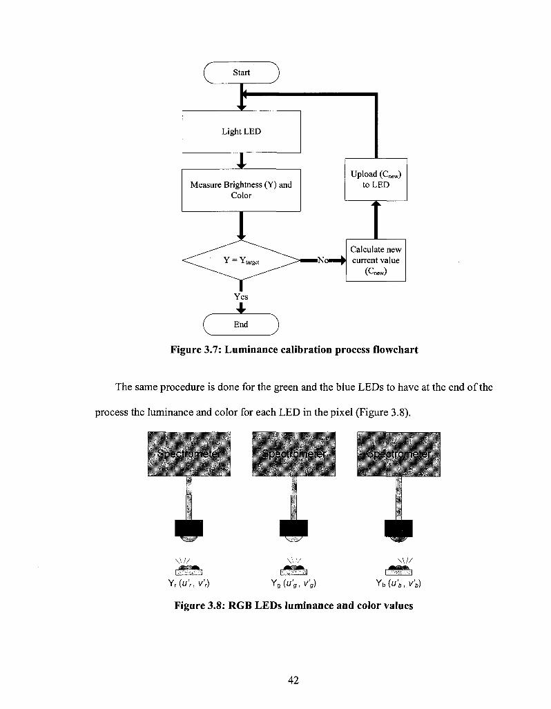
and Btarget)- Figure 3.9 illustrates the color correction concept.
. ^f , Rtarget
Measured \ wtarget """"" -%38S? Greens \ }6Sg / \
| / Measured \ Measured / Reds \ Whites , \ \ i \
\ / ^ - • B t a r g e ,
t
4 Measured
Blues
Figure 3.9: RGB LEDs luminance and color values
The proposed color correction algorithm is based on Grassman's laws of color
mixture. If two colors A and B are represented by points as shown in figure 3.10, then the
additive mixture of the two colors is represented by a new point C lying on the line
43

joining A and B. The position of C on the line depends on the forces exerted by A and B
(FA and FB), where these forces represent the relative luminance weights of A and B. It is
also at the center of gravity of each luminance weights. Hence the results are referred as
the Center of Gravity Law of Color Mixture which was announced by Isaac Newton.
Figure 3.10: The color C can be matched by an additive mixture
of the colors A & B.
The same concept applies when we have three colors R, G, and B represented by
points as shown in figure 3.11 then the additive mixture of the three colors is represented
by a new point W. The position of W depends on the relative luminance weights of R, G,
and B (The forces exerted by R, G, and B (FR, FQ, and FB)).
Accordingly, we conclude that the luminance weights are the main factors (forces) to
determine the color mixture point and not the luminance values themselves. Therefore the
proposed algorithm runs several steps to determine these factors and uses them to
calculate the correction coefficients. The coefficients will be uploaded to the LED matrix
board to perform the color correction (Color Rendering).
44
FR
\ \ *
W
*
Figure 3.11: The color W can be matched by an additive mixture
of the colors R, G, and B.
The algorithm utilizes the PWM correction methodology to implement the correction
process. In the following, we will explain the main vision of the color correction
algorithm, and later in this chapter we will explain different ways to implement the
algorithm according to the user available information and needs.
Algorithm inputs and outputs:
The algorithm has 14 inputs and 9 outputs. The inputs are represented by,
• Red LED chromaticity coordinates (u\, vV), and luminance (Yr)
• Green LED chromaticity coordinates (u 'g, v 'g), and luminance (Yg)
• Blue LED chromaticity coordinates (u 'b, v'/,), and luminance (Yb)
• White pixel chromaticity coordinates (u'w,v 'w), and luminance (Yw)
• Target Red chromaticity coordinates (u 'rt, v 'rJ), and luminance (Yr t)
• Target Green chromaticity coordinates (u 'gJ, v 'gJ), and luminance (Ygt)
• Target Blue chromaticity coordinates (u \j, v 'bj), and luminance (Yb_t)
45

The first eight inputs are measured and calculated in advance, and the last six inputs
should be provided by the user.
The outputs are represented by
• The red coefficients (Krr, Krg, and Krb)
• The green coefficients (K^, Kgg, and Kgb)
• The blue coefficients (Kbr, Kbg, and Kbb)
Where K^ represents the coefficient for the amount of row red in the target red, the Krg is
the coefficient for the amount of row red in the target green; the Krb is the coefficient for
the amount of row red in the target blue, and so on for the rest of the coefficients. The
formula for adjusting the video signal to each LED pixel is given by the following
equations;
R out = Krr + Krg + Krb
G out = Kgr + Kgg + Kgb o ~
B out = Kbr + Kbg + Kbb
Algorithm Steps
The following steps show the correction algorithm procedure for one pixel which applies
for the rest of the pixels in the LED matrix board. The procedure assumes that all the
target coordinates are inside the measured pixel Gamut, while later in this section we will
explain how the proposed algorithm deals with the out of gamut coordinates. It also
assumes that the pixels passed through the luminance calibration algorithm.
1. The color coordinates and luminance are measured for the saturated red (Yr
(u'r,v'r)), green (Yg (u'g,v'g)), blue (Yb (u'b,v'b)), and white (Yw (u'w,v'w)) (Figure
3.12).
46

Spectrometer Spectrometer Spectrometer Spectrometer
Yg{U'g, V'g) czrzj
Yb (u'n, v'b) Yw(u'w, v'w)
Figure 3.12: Saturated red, green, blue, and white measuring.
2. The red, green, and blue luminance weights (FR, FG, and FB) are calculated based
on the measured white color and on the fact that the sum of the luminance weights
equals to one (Figure 3.13).
("V>vs) v-
i i '
\
\ I \ ' F B
« ' » ' » ' \ i i ' t w/ r
(« '* , , V j )
/ (u'n. ,v'w)
(u'r,V'r)
Figure 3.13: Red, green and blue luminance weights (FR, FG, and FB).
3. The sub luminance weights are calculated for each color individually based on the
target color.
47

(.u'g.Vg)
*****a*^ ^ 'CJ*J. .» «.
(UrJ,V rj) ' / /
/ , ' FRR / •
\ I
= S«»^(«7,VJ,V;
Figure 3.14: Sub-luminance weights for target red, green and blue.
48
The calculated sub luminance weights are illustrated in figure 3.14 and listed as
follows;
• For target red : FRR, FGR, and FBR
• For target green : FRG, FGG, and FBG
• For target Blue : FRB, FGB, and FBB
4. The weights from step 2 with each set of the sub weights from step 3 are
combined to compute the coefficients for each color. The red coefficients (Kn-, Krg.
and Krb), the green coefficients (Kgr, Kgg, and Kgb), and the blue coefficients (Kt,r,
Kbg, and Kbb).
5. The algorithm checks the Luminance of each LED to determine whether the
coefficients of each set are sufficient to light up each color as the target luminance
(Yr_t, Yg t, Yb 0 or not. If the target luminance is not achieved with these
calculated coefficients, the algorithm calculates the error percentage and
multiplies it with the coefficients.
6. The algorithm runs coefficients unity check function to assure that the sum of each
set of coefficients does not exceed one.
Krr + Krg + Krb < 1
Kgr + Kgg + Kgb < 1 3 3
Kbr + Kbg + Kbb<\
If any set of the coefficients exceeds one, the algorithm calculates the error
percentage and multiplies it with the luminance for that color LED. The
luminance calibration algorithm will be run again to re-calibrate that LED
individually. The error percentage is also used to set the sum of those coefficients
at unity value.
49
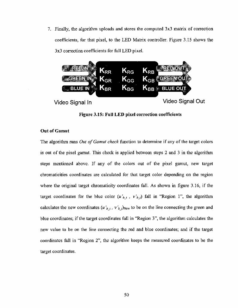
7. Finally, the algorithm uploads and stores the computed 3x3 matrix of correction
coefficients, for that pixel, to the LED Matrix controller. Figure 3.15 shows the
3x3 correction coefficients for full LED pixel.
Video Signal In Video Signal Out
Figure 3.15: Full LED pixel correction coefficients
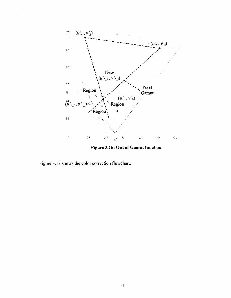
Out of Gamut
The algorithm runs Out of Gamut check function to determine if any of the target colors
is out of the pixel gamut. This check is applied between steps 2 and 3 in the algorithm
steps mentioned above. If any of the colors out of the pixel gamut, new target
chromaticities coordinates are calculated for that target color depending on the region
where the original target chromaticity coordinates fall. As shown in figure 3.16, if the
target coordinates for the blue color {u\j , v\j) fall in "Region 1", the algorithm
calculates the new coordinates (u 'b_t, v 'bjhiew to be on the line connecting the green and
blue coordinates; if the target coordinates fall in "Region 3", the algorithm calculates the
new value to be on the line connecting the red and blue coordinates; and if the target
coordinates fall in "Region 2", the algorithm keeps the measured coordinates to be the
target coordinates.
50
® Ini
&%
<3 -Q " -
<9 a
*$"
•3 s1
(u'b
$ r
En3
. . - («*-»* '*) - . .
i " - - * \ * • \ * * » • » \ • \ •
» New / \ ' \(u'bt,v'bt) / \
„ . \ • ' x -^ Pixel Region \ / /-.••'* •& » : v Gamut V * ( « 6 , V b)
' * o r, v'& /)''"::is.'"0\ Region /
A \ / • 'Region t 3 /
2 \ ** /
\ / ..\y
oi 0» ' , 03 oa on. [a]
Figure 3.16: Out of Gamut function
Figure 3.17 shows the color correction flowchart.
51
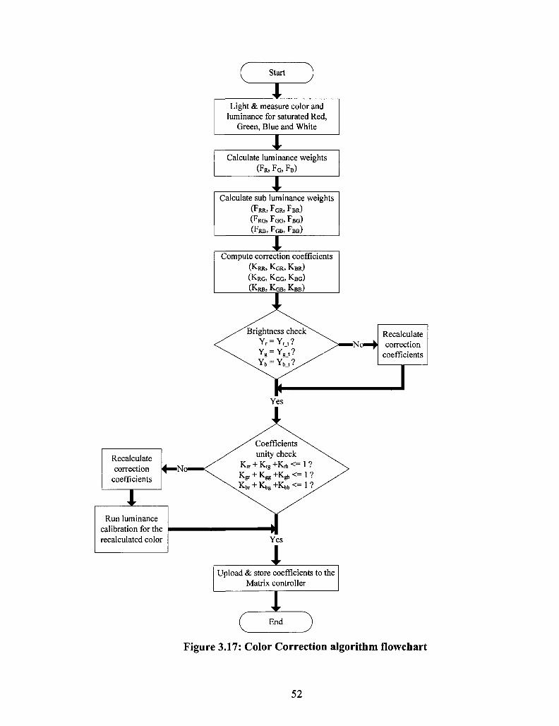
Start
Light & measure color and luminance for saturated Red,
Green, Blue and White
Calculate luminance weights (FR, FQ, F B )
Calculate sub luminance weights (FRR, FQ R ,
(FRG. FGG
(FRB, FQB,
FBR)
FBG)
FBB)
Recalculate correction
coefficients
Run luminance calibration for the recalculated color
Compute correction coefficients (KRR, KQR, KBR)
(KRG, KQG, KBG)
(KRB, KQB, KBB)
Yes
J,
Recalculate correction
coefficients
Upload & store coefficients to the Matrix controller
I End
Figure 3.17: Color Correction algorithm flowchart
52
3.4 Proposed Methodologies
Based on the algorithm mentioned in section 3.3, the following proposed methodologies
were developed to fit different users needs and according to the available inputs that can
be provided to the algorithm to perform the correction;
• RGBW Color and W Luminance methodology
• RGB Color and Luminance methodology
• W Color and Luminance methodology
• RGB Luminance methodology
• Achromatic Point methodology
Some of these methodologies' ideas are used by other industrial solutions available
in the market, like the RGB Color and Luminance methodology and the RGB Luminance
methodology. The RGB Color and Luminance methodology could provide a mediocre
resolution if the user didn't choose a suitable Luminance values to the algorithm to
calibrate and correct the colors. The RGBW color and W Luminance is developed to
calculate the needed Luminance values to the correction algorithm, which over come the
mediocre resolution that can be caused by the user. Later in this chapter, in the Image
Quality and Resolution section, the possible cause of mediocre resolution in corrected
and calibrated LED screens will be explained and discussed.
The methodologies can be useful for different user needs and can fit different
conditions. The following sub-sections will explain the methodologies' algorithms along
with the possible uses.
53
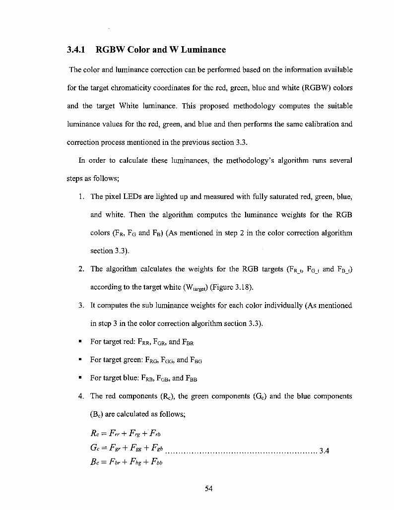
3.4.1 RGBW Color and W Luminance
The color and luminance correction can be performed based on the information available
for the target chromaticity coordinates for the red, green, blue and white (RGBW) colors
and the target White luminance. This proposed methodology computes the suitable
luminance values for the red, green, and blue and then performs the same calibration and
correction process mentioned in the previous section 3.3.
In order to calculate these luminances, the methodology's algorithm runs several
steps as follows;
1. The pixel LEDs are lighted up and measured with fully saturated red, green, blue,
and white. Then the algorithm computes the luminance weights for the RGB
colors (FR, FG and FB) (AS mentioned in step 2 in the color correction algorithm
section 3.3).
2. The algorithm calculates the weights for the RGB targets (FR t , FGJ and FB t)
according to the target white (Wtarget) (Figure 3.18).
3. It computes the sub luminance weights for each color individually (As mentioned
in step 3 in the color correction algorithm section 3.3).
• For target red: FRR, FGR, and FBR
• For target green: FRG, FGG, and FBG
• For target blue: FRB, FGB, and FBB
4. The red components (Re), the green components (Gc) and the blue components
(Bc) are calculated as follows;
Re = Frr + Frg + Frb
Gc = Fgr + Fgg + Fgb 3 4
Bc = Fbr + Fbg + Fbb
54
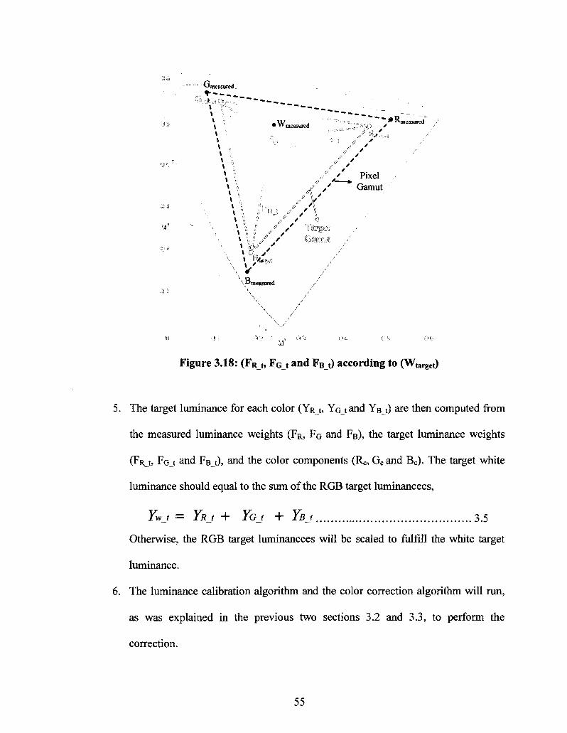
3 d u
Qt
Gracasured
t- .
\ \ \
» 6
\ t
t \ 1
Oi
• W m e a s u r e d
N ^ \ :
/? 0
\
\ TWaorecO I / *
s • V R / V-'measorai / \ /
\ / \ r
/ \ / \ / - v/
0 5 - „ 0 3
^ - —
~" -^ . ^ "-measured
'• , / ' " "
/ Pixel Gamut
0.0 01' l.
Figure 3.18: (FR t, FG t and FB t) according to (Wtarget)
5. The target luminance for each color (YR_t, YGJ and YB J) are then computed from
the measured luminance weights (FR, FQ and FB), the target luminance weights
(FRJ, FGJ and FBJ), and the color components (Re, Gc and Bc). The target white
luminance should equal to the sum of the RGB target luminancees,
= YRt+ Yat + Ynt „ 3.5
Otherwise, the RGB target luminancees will be scaled to fulfill the white target
luminance.
6. The luminance calibration algorithm and the color correction algorithm will run,
as was explained in the previous two sections 3.2 and 3.3, to perform the
correction.
55
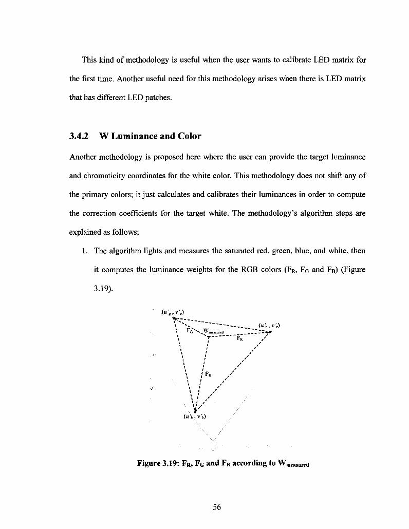
This kind of methodology is useful when the user wants to calibrate LED matrix for
the first time. Another useful need for this methodology arises when there is LED matrix
that has different LED patches.
3.4.2 W Luminance and Color
Another methodology is proposed here where the user can provide the target luminance
and chromaticity coordinates for the white color. This methodology does not shift any of
the primary colors; it just calculates and calibrates their luminances in order to compute
the correction coefficients for the target white. The methodology's algorithm steps are
explained as follows;
1. The algorithm lights and measures the saturated red, green, blue, and white, then
it computes the luminance weights for the RGB colors (FR, FG and FB) (Figure
3.19).
* **G **xWmeasure<! _ _ — - - - — ***
Figure 3.19: FR, FG and FB according to WmeAsurea
56
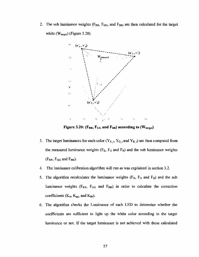
2. The sub luminance weights (FRR, FQQ, and FBB> are then calculated for the target
white (Wtarget) (Figure 3.20).
:" (««>v'«) t?
\"p% («'„v',) •.i * \ " m e a s u r e d .----- ~AJr
\
\
> , > • „ /
V » .? /
\ « /
(«\.v'») /
\ /
\ y u"
Figure 3.20: (FRR, FGG and FBB) according to (Wtarget)
3. The target luminances for each color (YR t, YG tand YB t) are then computed from
the measured luminance weights (FR, FQ and FB) and the sub luminance weights
(FRR, FOG and FBB).
4. The luminance calibration algorithm will run as was explained in section 3.2.
5. The algorithm recalculates the luminance weights (FR, FG and FB) and the sub
luminance weights (FRR, FQG and FBB) in order to calculate the correction
coefficients (KR, Kgg, and Kt>b).
6. The algorithm checks the Luminance of each LED to determine whether the
coefficients are sufficient to light up the white color according to the target
luminance or not. If the target luminance is not achieved with these calculated
57
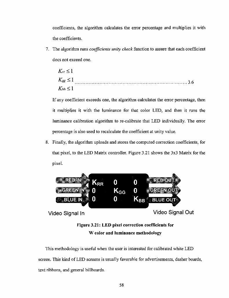
coefficients, the algorithm calculates the error percentage and multiplies it with
the coefficients.
7. The algorithm runs coefficients unity check function to assure that each coefficient
does not exceed one.
Krr<\
Kss^ 3.6
Kbb<\
If any coefficient exceeds one, the algorithm calculates the error percentage, then
it multiplies it with the luminance for that color LED, and then it runs the
luminance calibration algorithm to re-calibrate that LED individually. The error
percentage is also used to recalculate the coefficient at unity value.
8. Finally, the algorithm uploads and stores the computed correction coefficients, for
that pixel, to the LED Matrix controller. Figure 3.21 shows the 3x3 Matrix for the
pixel.
Video Signal In Video Signal Out
Figure 3.21: LED pixel correction coefficients for
W color and luminance methodology
This methodology is useful when the user is interested for calibrated white LED
screen. This kind of LED screens is usually favorable for advertisements, dasher boards,
text ribbons, and general billboards.
58
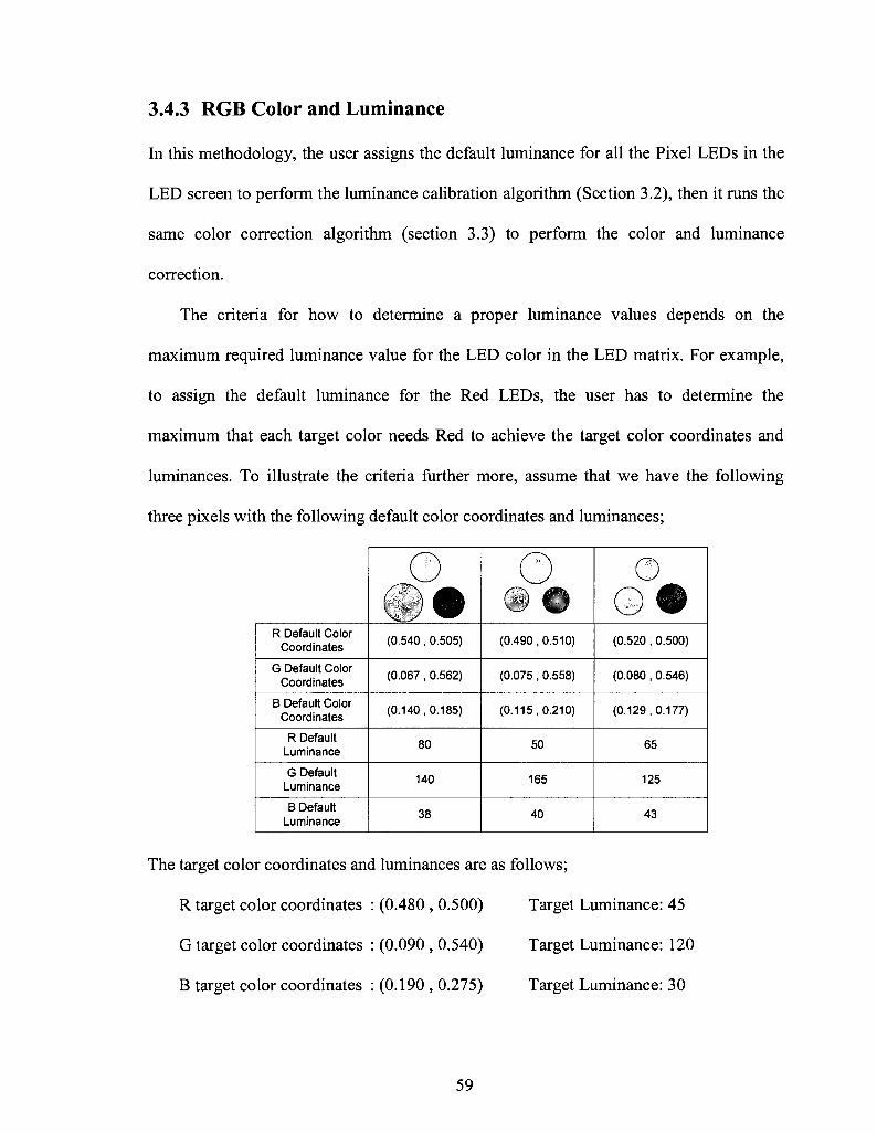
3.4.3 RGB Color and Luminance
In this methodology, the user assigns the default luminance for all the Pixel LEDs in the
LED screen to perform the luminance calibration algorithm (Section 3.2), then it runs the
same color correction algorithm (section 3.3) to perform the color and luminance
correction.
The criteria for how to determine a proper luminance values depends on the
maximum required luminance value for the LED color in the LED matrix. For example,
to assign the default luminance for the Red LEDs, the user has to determine the
maximum that each target color needs Red to achieve the target color coordinates and
luminances. To illustrate the criteria further more, assume that we have the following
three pixels with the following default color coordinates and luminances;
R Default Color Coordinates
G Default Color Coordinates
B Default Color Coordinates
R Default Luminance
G Default Luminance
B Default Luminance
© (0.540 , 0.505)
(0.067 , 0.562)
(0.140 , 0.185)
80
140
38
o (0.490 , 0.510)
(0.075 , 0.558)
(0.115,0.210)
50
165
40
© © • (0.520 , 0.500)
(0.080 , 0.546)
(0.129,0.177)
65
125
43
The target color coordinates and luminances are as follows;
R target color coordinates : (0.480 , 0.500) Target Luminance: 45
G target color coordinates : (0.090 , 0.540) Target Luminance: 120
B target color coordinates : (0.190 , 0.275) Target Luminance: 30
59
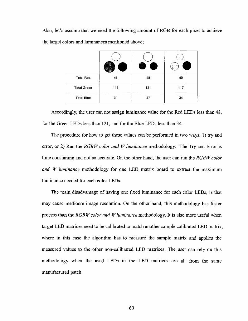
Also, let's assume that we need the following amount of RGB for each pixel to achieve
the target colors and luminances mentioned above;
Total Red
Total Green
Total Blue
o 45
115
31
o • •
48
121
27
0 © •
40
117
34
Accordingly, the user can not assign luminance value for the Red LEDs less than 48,
for the Green LEDs less than 121, and for the Blue LEDs less than 34.
The procedure for how to get these values can be performed in two ways, 1) try and
error, or 2) Run the RGB W color and W luminance methodology. The Try and Error is
time consuming and not so accurate. On the other hand, the user can run the RGB W color
and W luminance methodology for one LED matrix board to extract the maximum
luminance needed for each color LEDs.
The main disadvantage of having one fixed luminance for each color LEDs, is that
may cause mediocre image resolution. On the other hand, this methodology has faster
process than the RGBWcolor and Wluminance methodology. It is also more useful when
target LED matrices need to be calibrated to match another sample calibrated LED matrix,
where in this case the algorithm has to measure the sample matrix and applies the
measured values to the other non-calibrated LED matrices. The user can rely on this
methodology when the used LEDs in the LED matrices are all from the same
manufactured patch.
60

3.4.4 RGB Luminance
The RGB luminance methodology uses only the Luminance Calibration process which
calibrates the pixels LEDs to target luminances without performing any color correction.
This methodology reduces the non-uniformity problems in the LED screens, but it does
not solve it.
This process can be useful for LED lighting products as they are usually apart and do
not need accurate color calibration. It is also used for LED screens when a fast calibration
is needed.
3.4.5 Achromatic Point
The achromatic point methodology was developed for LED lighting products, as this
methodology calibrate the white achromatic point with the maximum possible luminance.
The methodology is similar to that White luminance and color algorithm with one main
difference that it does not calibrate the luminance.
The methodology's algorithm is performed in few steps as follows;
1. The algorithm lights and measures the pixel with fully saturated red, green, blue,
and white, then it computes the luminance weights for the RGB colors (FR, FG and
FB).
2. The sub luminance weights (FRR, FGG, and FBB) are calculated for the target white.
3. The luminance weights (FR, FG and FB) and the sub luminance weights (FRR, FGG
and FBB) are used to calculate the correction coefficients (Kn-, Kgg, and Kbb).
61
4. Finally, the algorithm uploads and stores the computed correction coefficients, for
that pixel, to the LED Matrix controller.
3.5 Image Quality and Resolution
LED video screen image quality and resolution influence the consumers' decision with
the wide choices available in the market. The image quality can be solved through the
color correction and calibration process, but it is not usually necessary to have high
resolution associate with the correction process, and that all depends on the algorithm and
the methodology used to correct and calibrate the LED screens. In this section, the Image
Quality and Resolution provided by the methodologies, RGB color and Luminance and
RGBW Color and WLuminance, will be discussed.
To illustrate how each of the two mentioned methodologies influence the Resolution
of the image, assume that we have LED pixel with the following default RGB color and
luminance;
Yr - 140 nits, (u'r = 0.52, v \ = 0.54)
Yg = 230 nits, (u'g = 0.09, v'g = 0.58)
Yb = 60nits, (u'b = 0.15, v'b= 0.21)
And we wish to correct the pixel colors as the following;
Red target color coordinates : (0.490, 0.510) Target luminance: 90 nits
Green target color coordinates : (0.100, 0.550) Target luminance: 170 nits
Blue target color coordinates : (0.180, 0.270) Target luminance: 30 nits
The RGBW color and W luminance methodology will proceed as the following;
62
First, it calculates the proper luminance for each LED individually and then it will run the
Luminance Calibration Process. The new calculated luminance (assumption) will be as
the following;
Yr = 98 nits
Yg= 176 nits
Yb = 32 nits
Then, the algorithm calculates the coefficients to correct the color and luminance and
uploads them.
Total Luminance R = (0.925 x 98)R + (0.011 x 176)G + (0.075 x 32)B = 95 nits
Total Luminance G = (0.009 x 98)R + (0.948 x 176)G + (0.068 x 32)B = 170 nits
Total Luminance B = (0.029 x 98)R + (0.007 x 176)G + (0.810 x 32)B = 30 nits
The calculated coefficients will be as the following (Figure 3.22);
Video Signal In Video Signal Out
Figure 3.22: LED pixel correction coefficients for
RGBW color and W luminance methodology example
For the RGB color and luminance methodology will proceed as the following;
First, the user is going to assign one default luminance value for each LED color for the
LED pixels in the LED screen. Assume that the assigned luminance values are as the
following;
Y r= 115 nits
63

Yg = 205 nits
Yb = 40 nits
Then, the algorithm will run the Luminance Calibration Process and calculates the
coefficients to correct the color and luminance and uploads them.
Total Luminance R = (0.753 x 115)R + (0.024 x 205)G + (0.088 x 40)B = 95 nits
Total Luminance G = (0.071 x 115)R + (0.787 x 205)G + (0.012 x 40)B = 170 nits
Total Luminance B = (0.014 x 115)R + (0.009 x 205)G + (0.665 x 40)B = 30 nits
The calculated coefficients will be as the following (Figure 3.23);
Video Signal In Video Signal Out
Figure 3.23: LED pixel correction coefficients for
RGB color and luminance methodology example
Reviewing the results out of the two methodologies example mentioned above, the
RGB W color and W Luminance methodology shows higher efficiency and resolution for
the corrected pixel as shown in table 3.1.
The RGB Color and Luminance methodology can provide a better resolution if the
determined luminance values were closer to the ones provided by the RGBW Color and
WLuminance methodology.
64
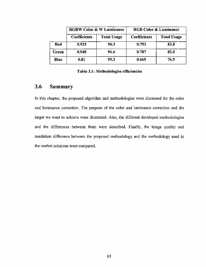
Red
Green
Blue
RGBW Color & W Luminance
Coefficients
0.925
0.948
0.81
Total Usage
96.3
96.6
95.3
RGB Color & Luminance
Coefficients
0.753
0.787
0.665
Total Usage
83.8
82.0
76.5
Table 3.1: Methodologies efficiencies
3.6 Summary
In this chapter, the proposed algorithm and methodologies were discussed for the color
and luminance correction. The purpose of the color and luminance correction and the
target we want to achieve were illustrated. Also, the different developed methodologies
and the differences between them were described. Finally, the image quality and
resolution difference between the proposed methodology and the methodology used in
the market solutions were compared.
65
CHAPTER 4
Correction and Calibration Experimental
Setup
4.1 Introduction
A LED Screen Correction and Calibration System is developed for measuring and
correcting the color and luminance of each LED in every pixel, in a LED video screen,
and stores the correction data in lookup tables in the LED matrix memory. The system is
an integrated hardware and software solution where it uses; 1) robotic spectrometer head,
to precisely measure the chromaticity and luminance of each LED in a target LED Matrix,
and 2) Windows based graphical user interface (GUI) application software, to calculate
the correction coefficients and factors for each pixel based on the measured data.
4.2 System Description
The proposed Correction and Calibration System consists of three components:
• Robotic Spectrometer system which uses off-the-shelf Robot (JR2500 by Janome)
and Spectrometer (SPM-002-A by Photon Control).
• Correction Software which is developed using VB.net.
• Matrix Controller which provides full control over the LED matrix (see section
2.1.5 for more details).
The system can be used to calibrate different LED matrix sizes with up to 16x16/28
mm pitch. It has precision correction with pixel-to-pixel luminance corrected to +/- 3%
66
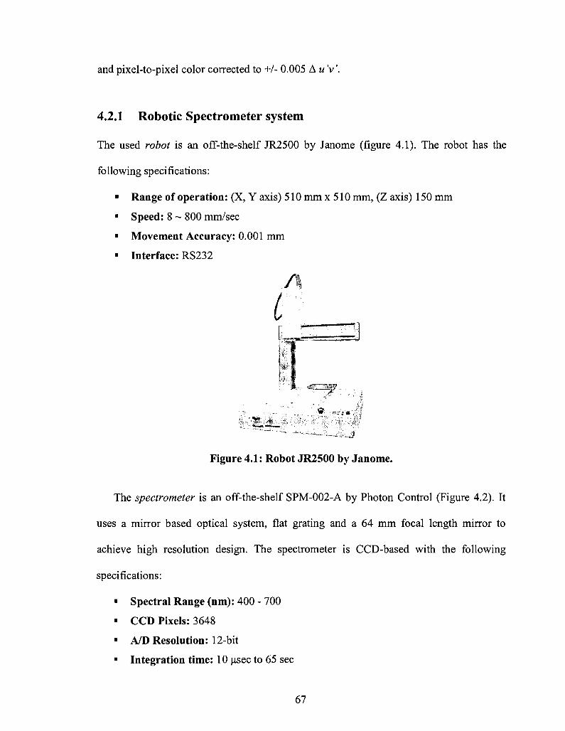
and pixel-to-pixel color corrected to +/- 0.005 A w V.
4.2.1 Robotic Spectrometer system
The used robot is an off-the-shelf JR2500 by Janome (figure 4.1). The robot has the
following specifications:
• Range of operation: (X, Y axis) 510 mm x 510 mm, (Z axis) 150 mm
• Speed: 8 ~ 800 mm/sec
• Movement Accuracy: 0.001 mm
• Interface: RS232
• • - v . ~ - * - ~ - : . . ^ ^ _ ^ \ ^ ^ ^
Figure 4.1: Robot JR2500 by Janome.
The spectrometer is an off-the-shelf SPM-002-A by Photon Control (Figure 4.2). It
uses a mirror based optical system, flat grating and a 64 mm focal length mirror to
achieve high resolution design. The spectrometer is CCD-based with the following
specifications:
• Spectral Range (nm): 400 - 700
• CCD Pixels: 3648
• A/D Resolution: 12-bit
• Integration time: 10 usee to 65 sec
67

• Interface: USB 2.0
Figure 4.2: Spectrometer SPM-002-A by Photon Control
A cosine receptor (diffuser) is used and attached to the spectrometer fiber head to
collect and diffuse the input light. The receptor provides accurate absolute intensity when
multiple lights are to be measured at the same time.
Figure 4.3 shows the light measuring path inside the spectrometer. The spectrometer
measures the light's spectral power frequently according to the set integration time
(Exposure time), for the wavelength range 400 nm to 700 nm, and stores the data on a
lookup table memory. The stored data represents the SPD which is used to determine the
light's color and luminance.
Gptx^ component &ay<ust Spectral Power Data
/ 400 / 400.06
400.16
699.82 699.92 700
ColNmstm? functiw Feeing fenaan
Figure 4.3: Light measuring path inside the spectrometer.
(Optical layout drawing from http://www.hamamatsu.com)
68

The receptor along with the spectrometer fiber is attached with a custom fitting to the
robot Z-axis arm, and the LED Matrix is placed with a custom base on the robot X-axis
base. Figure 4.4 shows a picture of the robotic spectrometer system.
*nnr ' _:N
Figure 4.4: Robotic Spectrometer system
4.2.2 Correction Software
The robot, the spectrometer, and the LED matrix controller interfaces communicate with
the correction software which in turn is controlling all over the system to run the
correction process.
The Software is built out of several classes (figure 4.5) which represent a set of
objects. Each of the hardware components (The robot, the spectrometer, and the matrix
controller) has one control class that works as software driver. These drivers are
responsible for communication link initialization, hardware initialization, and building,
sending, receiving and checking commands. As for the other classes, there is a class
responsible for the CIE chromaticity coordinates and luminance calculations, other
69

classes are available for each LED matrix type which has the matrix type, size, pitch,
position, memory map, and the communication commands.
Solution Explorer - MatrrK_Robot_Sensor
MatriK_Robot Sensor M[ [aj My Project
j - § CIE_Class.vb | Q CIE1931_XYZ_Class.vb {•••• | f l ColorMixingform.vb !••• § ] DataTableForm.vb !•••• ^3 GM_16_5_Class.vb !•••• £§| IMatrix.vb !•• Q JR2503N_Class.vb i" | 3 MainForm.vb !••• | 3 PMjClass.vb !•••• ^ 5PM002A_Class.vb L ;J3 VLite_Class,vb
^Solution Explorer j ^Da ta Sources |f^Properties
Figure 4.5: Software classes
Figure 4.6 shows the software Main window. Clicking the Auto Connect (Auto
Disconnect) button makes the software to search, communicate, and connect (disconnect)
with the system hardware automatically without the need to specify the communication
port numbers. The user has to select the type of the LED Matrix from the LED Matrix
combo list. Clicking the initialize button will; 1) Create the LED Matrix object and load
the Matrix configuration data, 2) power on and initialize the robot, 3) initialize the Matrix
controller, and 4) set the spectrometer exposure time. The robot status, the matrix
controller status, and the spectrometer status descriptions are always briefly shown at the
bottom of the software window. As it is shown in the main tab, the software can run
different correction algorithms based on the available correction information and the user
need. The algorithms were explained in the previous chapter.
70
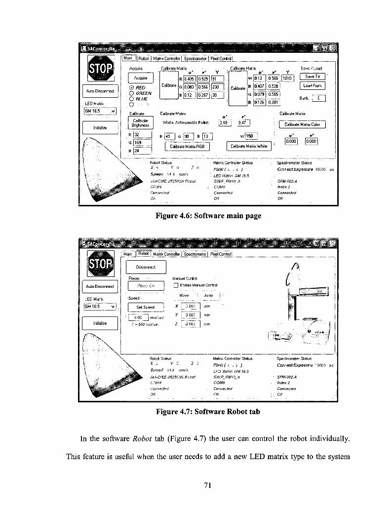
Si SAConcordia
Auto Disconnect
LED Matrix
GM16.5
Main J! Robot j| Matrix Controller | Spectrometer! Pixel Control)
Acquire Calibrate Matrix Calibrate Matrix
Acquire
© RED O GREEN O BLUE
o .••-..-
Calibrate
Calibrate
R[0.405[ [0.525 | [51 j
GJ0.0S3 110.566 11230 \. B l°-i27l I°^L\ W \
Calibrate
u'
VI ] 0.13
R 10.407
G 10.079
B 16T126
v'
10.506
0.528
j 0.565]
[6.281""
y J1010 |
Save / Load
Save To
Load From
Calibrate Brightness
*KI3 G fl69 ]
B |24 |
Calibrate Matrix
Wisite Achromatic Point:
Bank
Calibrate Matrix
0.19 0.47 Calibrate Matrix Color
R 45 G 90 B 13 w!150
Calibrate Matrix RGB Calibrate Matrix White [OJDOO]
Robot Status
x 0 v 0 2 c
Speed 14.4 x/m's
JANQME JR2503N Rabat
COM4
Connected
OK
Matrix Controller Status
Pixel ( x . y j
LED Matrix S.« f 6.5 SXVP_PimO_A COM3
Connected OK
Spectrometer Status
Current Exposure 10000 us
SPM-002-A Index 2 Connected OK
Figure 4.6: Software main page
lEjui Ma 'n L _ _ i Matrix Controller j| Spectrometer | Pixel Control
Manual Control
I j Enable Manual Control c: Move
X 0 000 1
Y
1
0.000 j
0.000 |
Jump
mm
mm
I 3&r
Robot Status
X 0 Y 0 Z 0
Speeil 14.4 mat's
MlMOME JP.250M Robot
COM4
Connected OK
Matrix Controller Status
Pixei ( x , y J
LED Matrix GM J 6.5
com Connected OK
Spectrometer Status
Current Exposure 10000 us
SPM-002-A index 2 Connected OK
Figure 4.7: Software Robot tab
In the software Robot tab (Figure 4.7) the user can control the robot individually.
This feature is useful when the user needs to add a new LED matrix type to the system
71
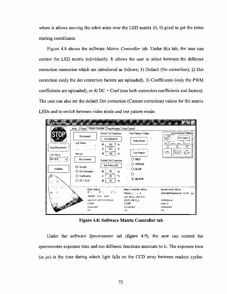
where it allows moving the robot arms over the LED matrix (0, 0) pixel to get the robot
starting coordinates.
Figure 4.8 shows the software Matrix Controller tab. Under this tab, the user can
control the LED matrix individually. It allows the user to select between the different
correction memories which are introduced as follows; 1) Default (No correction), 2) Dot
correction (only the dot correction factors are uploaded), 3) Coefficients (only the PWM
coefficients are uploaded), or 4) DC + Coef (run both correction coefficients and factors).
The user can also set the default Dot correction (Current correction) values for the matrix
LEDs and to switch between video mode and test pattern mode.
Figure 4.8: Software Matrix Controller tab
Under the software Spectrometer tab (figure 4.9), the user can control the
spectrometer exposure time and run different functions associate to it. The exposure time
(in JUS) is the time during which light falls on the CCD array between readout cycles.
72

Adjusting this parameter changes the overall sensitivity of the instrument, as changing
the exposure does for a camera.
Figure 4.9: Software Spectrometer tab
Other features, such as Pixel Binning, Time Average, Black Level measurement, and
Diffuser Correction, were developed and implemented for the correction process to have
accurate readings and higher signal-to-noise ratio (SNR). The following are brief
descriptions for each of these features;
• Pixel Binning: is a technique that averages across spectral data. This technique
averages a group of adjacent detector elements. A value of 5, for example,
averages each data point with 5 points to its left and 5 points to its right. The
greater this value, the smoother the data and the higher the SNR. If the value
entered is too high, a loss in spectral resolution will result. The SNR will improve
by the square root of the number of pixels averaged.
73
• Time Average: Sets the number of discrete spectral acquisitions that are
accumulated by the spectrometer before the software calculates the light
chromaticity and luminance. The higher the value, the better the SNR. Very large
scan numbers can be averaged, but this can easily cause total data collection times
to approach 5 - 1 0 minutes and longer.
• Black Level: The black level reference is taken with the light source off. The
Black Level function stores a background scan which will be subtracted from
subsequent data scans for computing irradiance. The CCD sensor array is an
integrating sensor; that is, charge is accumulated continuously in each of the CCD
pixels until removed during a readout cycle. The charge desired is that due to the
optical signal under observation. However, other sources also cause charge to
accumulate between readout cycles, acting as a background or pedestal signal
which varies slightly from pixel to pixel. There are three primary sources for dark
signal: detector dark current, light scattered within the instrument, and ambient
light in the test area. Usually the most important of these is detector dark current,
which can be very significant for integration times of 300 mSec and longer. Every
time the integration period is changed, a new Black Level must be taken.
• Diffuser Correction: It is a function to calibrate the spectrometer data with the use
of a diffuser. It measures a white reference light without the existence of the
diffuser, and stores the spectral power amplitudes at each wavelength in a look up
table. The software asks the user to mount the diffuser to measure the reference
light again and to compare both results to produce the diffuser correction table.
74
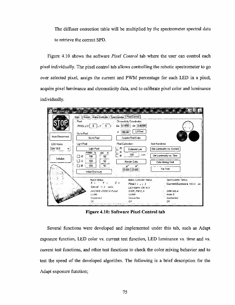
The diffuser correction table will be multiplied by the spectrometer spectral data
to retrieve the correct SPD.
Figure 4.10 shows the software Pixel Control tab where the user can control each
pixel individually. The pixel control tab allows controlling the robotic spectrometer to go
over selected pixel, assign the current and PWM percentage for each LED in a pixel,
acquire pixel luminance and chromaticity data, and to calibrate pixel color and luminance
individually.
Figure 4.10: Software Pixel Control tab
Several functions were developed and implemented under this tab, such as Adapt
exposure function, LED color vs. current test function, LED luminance vs. time and vs.
current test functions, and other test functions to check the color mixing behavior and to
test the speed of the developed algorithm. The following is a brief description for the
Adapt exposure function;
75
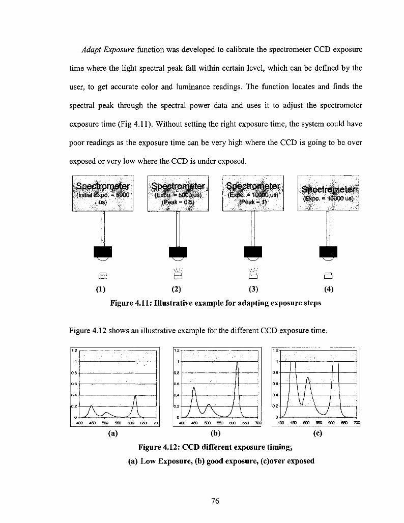
Adapt Exposure function was developed to calibrate the spectrometer CCD exposure
time where the light spectral peak fall within certain level, which can be defined by the
user, to get accurate color and luminance readings. The function locates and finds the
spectral peak through the spectral power data and uses it to adjust the spectrometer
exposure time (Fig 4.11). Without setting the right exposure time, the system could have
poor readings as the exposure time can be very high where the CCD is going to be over
exposed or very low where the CCD is under exposed.
Specjromger (Initial Expo. = 5000
us)
Spectrometer (Expo. = 10000 us)
B B r—n i i r~~i r~n
(1) (2) (3) (4)
Figure 4.11: Illustrative example for adapting exposure steps
Figure 4.12 shows an illustrative example for the different CCD exposure time.
400 450 500 550 600 650 700 400 450 500 550 600 650 700
. „
1
0.8
0.6
0.4
0.2
4(
l /
1TTT \1\ I
J V 7 V » 450 500 550 600 650 7( X
(a) (b) (c)
Figure 4.12: CCD different exposure timing;
(a) Low Exposure, (b) good exposure, (c)over exposed
76
4.3 Color and Luminance Correction and Calibration Process
The proposed color and luminance correction methodology consists of several software
and hardware steps. These steps are arranged in the following sequence:
First, system initialization; where the software searches, connects, and resets the system's
hardware components. Second, the user has to select the LED Matrix type which allows
the software to generate and load the matrix board configurations (size, pitch, memory
map, and starting coordinates). Third, the robotic spectrometer head moves over the first
pixel (0, 0), which will be used as a reference light, to set the spectrometer exposure time
using the Adapt Exposure function. (Note: we used the first pixel as a reference light for
research and development purposes only. The reference light should be a separate unit).
Fourth, the software runs the Luminance calibration process where it calibrates the
luminance for each LED (Red, Green, and Blue) individually and generates the
luminance calibration factors. Fifth, the software runs the color correction algorithm to
compute a 3x3 matrix of correction functions for the pixel. Sixth, the system stores the
coefficients and factors in the matrix controller. Finally, the robot spectrometer head
moves to the next pixel to run the luminance and color correction algorithm again. Figure
4.13 shows a flowchart for the proposed methodology.
77
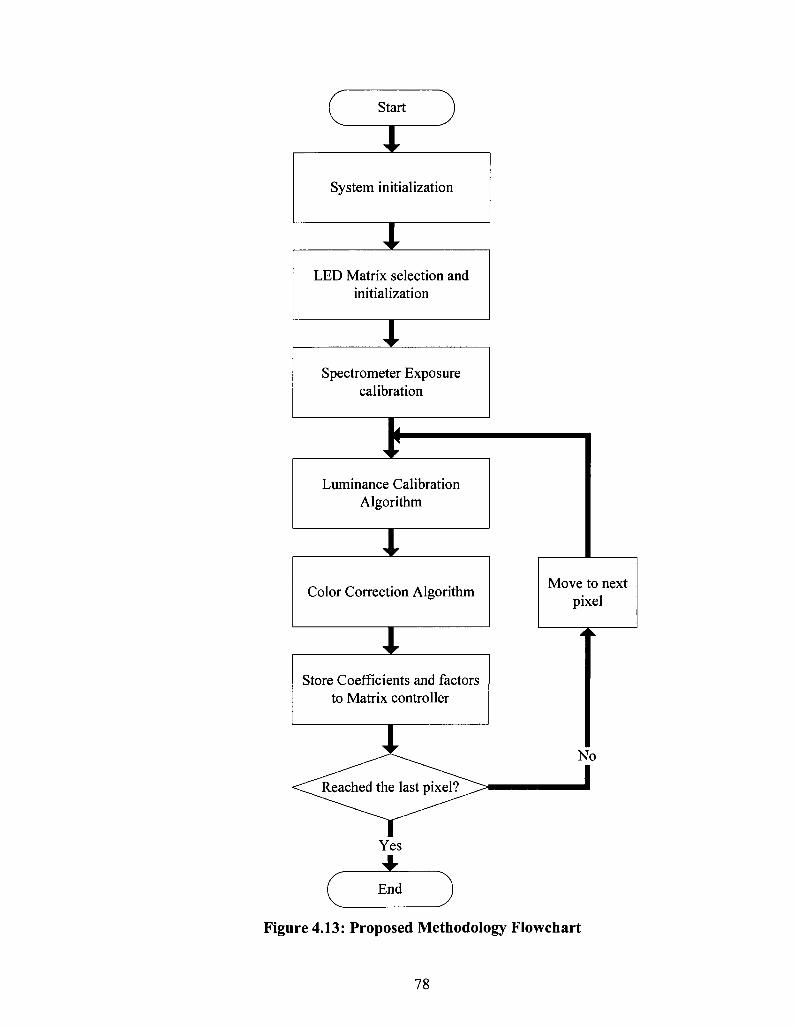
Start
System initialization
LED Matrix selection and initialization
Spectrometer Exposure calibration
I Luminance Calibration
Algorithm
Color Correction Algorithm
Store Coefficients and factors to Matrix controller
Move to next pixel
No
J
Figure 4.13: Proposed Methodology Flowchart
78
4.4 Summary
In this chapter, we described in details the developed color and luminance correction and
calibration experimental system components, structure, and integration along with the
over all specifications and the application software to implement and test our proposed
algorithms and technique.
79
CHAPTER 5
Experimental Results
5.1 Experiments Set Up
The following experiments are designed in order to verify the functionality of the
proposed algorithms. A 16x16 / 16.5mm pitch LED matrix board is used; each pixel
consists of surface mount device (SMD) RGB LEDs. LEDs are driven by LED drivers
with a maximum current set for each color LED in each pixel as the following;
• Red max. current = 40 mA
• Green max. current = 40 mA
• Blue max. current = 40 mA
The default current is set for each color LED in each pixel as the following;
• Red default current = 25%
• Green default current = 29%
• Blue default current = 28%
The spectrometer exposure time was fixed to 200 ms.
Since each board has a large amount of pixels (256 pixels), the experiments will
show a sample results of 16 measured, calibrated, and corrected pixels. The experiments
will illustrate the results of the following three methodologies;
- RGBW Color and W Brightness
80
- RGB Color and Brightness
- RGB Brightness
Each experiment will provide a table with the default values for the color coordinates
and luminance for each LED in each pixel associated with the calibrated current and
luminance values, and the corrected color coordinates and luminance values. The
experiments will also provide a table for the correction coefficients associate with the
usage efficiency for the calibrated LEDs. The coefficients with the usage efficiency will
show the different in the resolution between the different methodologies used for the
correction. Several diagrams will be provided as well to show the position of the
measured data and the corrected data for each color.
5.2 RGBW Color and W luminance Experiment
For this experiment we had the following target color coordinates and luminance;
White target color coordinates : u' = 0.175, v' = 0.490. Target luminance: 230.
Red target color coordinates : u' = 0.485, v' = 0.500
Green target color coordinates : u' = 0.090, v' = 0.560
Blue target color coordinates : u' = 0.150, v' = 0.250
Table 5.1 shows the results for the default, calibrated, and corrected data. Table 5.2
shows a summary for the minimum, maximum, and average values for each color. Table
5.3 shows the coefficients for each pixel and the used percentage from each calibrated
LED. Table 5.4 shows a summary for the maximum, minimum, and average usage
efficiency for the proposed methodology.
81
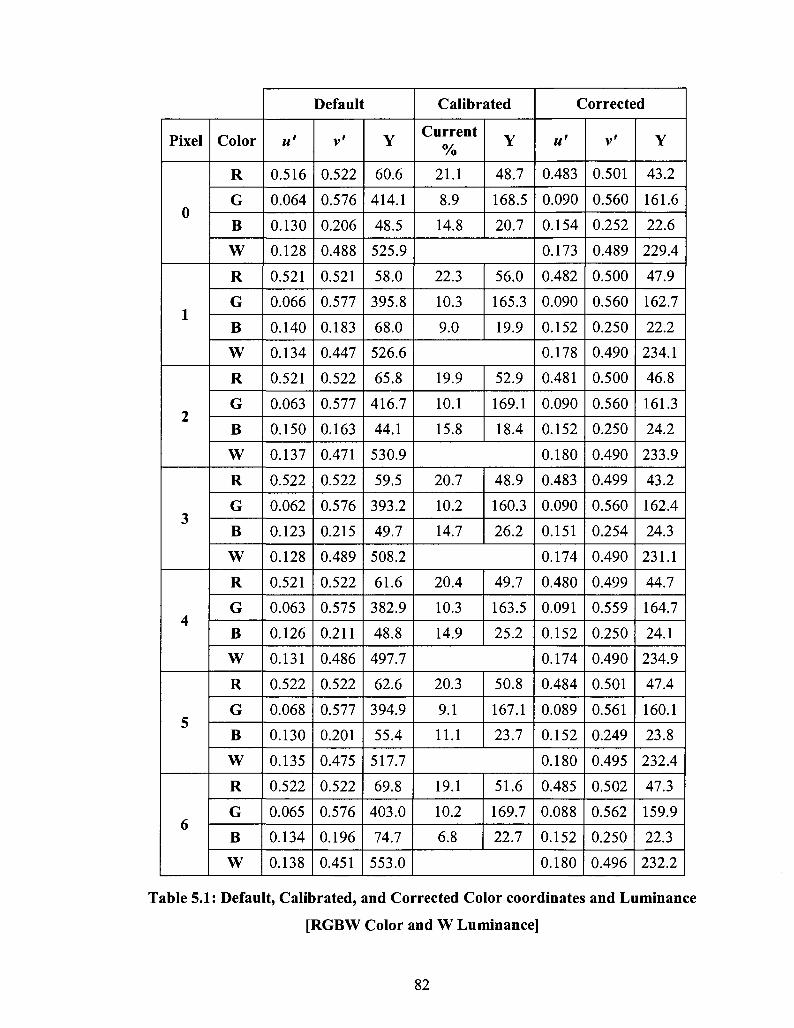
Pixel
0
1
2
3
4
5
6
Color
R
G
B
W
R
G
B
W
R
G
B
W
R
G
B
W
R
G
B
W
R
G
B
W
R
G
B
W
Default
u'
0.516
0.064
0.130
0.128
0.521
0.066
0.140
0.134
0.521
0.063
0.150
0.137
0.522
0.062
0.123
0.128
0.521
0.063
0.126
0.131
0.522
0.068
0.130
0.135
0.522
0.065
0.134
0.138
v'
0.522
0.576
0.206
0.488
0.521
0.577
0.183
0.447
0.522
0.577
0.163
0.471
0.522
0.576
0.215
0.489
0.522
0.575
0.211
0.486
0.522
0.577
0.201
0.475
0.522
0.576
0.196
0.451
Y
60.6
414.1
48.5
525.9
58.0
395.8
68.0
526.6
65.8
416.7
44.1
530.9
59.5
393.2
49.7
508.2
61.6
382.9
48.8
497.7
62.6
394.9
55.4
517.7
69.8
403.0
74.7
553.0
Calibrated
Current %
21.1
8.9
14.8
Y
48.7
168.5
20.7
22.3
10.3
9.0
56.0
165.3
19.9
19.9
10.1
15.8
52.9
169.1
18.4
20.7
10.2
14.7
48.9
160.3
26.2
20.4
10.3
14.9
49.7
163.5
25.2
20.3
9.1
11.1
50.8
167.1
23.7
19.1
10.2
6.8
51.6
169.7
22.7
Corrected
« '
0.483
0.090
0.154
0.173
0.482
0.090
0.152
0.178
0.481
0.090
0.152
0.180
0.483
0.090
0.151
0.174
0.480
0.091
0.152
0.174
0.484
0.089
0.152
0.180
0.485
0.088
0.152
0.180
v'
0.501
0.560
0.252
0.489
0.500
0.560
0.250
0.490
0.500
0.560
0.250
0.490
0.499
0.560
0.254
0.490
0.499
0.559
0.250
0.490
0.501
0.561
0.249
0.495
0.502
0.562
0.250
0.496
Y
43.2
161.6
22.6
229.4
47.9
162.7
22.2
234.1
46.8
161.3
24.2
233.9
43.2
162.4
24.3
231.1
44.7
164.7
24.1
234.9
47.4
160.1
23.8
232.4
47.3
159.9
22.3
232.2
Table 5.1: Default, Calibrated, and Corrected Color coordinates and Luminance
[RGBW Color and W Luminance]
82

Pixel
7
8
9
10
11
12
13
Color
R
G
B
W
R
G
B
W
R
G
B
W
R
G
B
W
R
G
B
W
R
G
B
W
R
G
B
W
Default
u'
0.521
0.071
0.132
0.138
0.522
0.072
0.132
0.142
0.520
0.067
0.135
0.135
0.521
0.064
0.131
0.130
0.521
0.066
0.115
0.130
0.521
0.065
0.148
0.140
0.519
0.068
0.151
0.141
v'
0.521
0.576
0.198
0.475
0.522
0.573
0.198
0.469
0.522
0.574
0.195
0.444
0.522
0.575
0.200
0.482
0.521
0.576
0.232
0.501
0.522
0.574
0.168
0.461
0.522
0.577
0.164
0.479
Y
64.9
397.9
54.7
522.1
63.6
367.4
53.6
489.1
62.3
395.1
77.4
540.6
64.1
424.2
52.5
544.7
63.2
405.0
48.2
521.1
64.8
387.1
48.5
505.1
61.1
374.5
35.7
474.4
Calibrated
Current %
18.8
9.0
11.2
Y
47.7
166.7
23.7
19.3
10.1
11.8
46.5
166.2
23.4
20.3
8.9
7.0
50.0
169.8
23.5
20.4
8.7
11.7
51.6
179.7
22.8
19.0
9.1
13.0
49.8
169.2
23.0
20.2
9.2
11.6
52.5
167.4
22.8
21.7
9.4
17.1
50.1
162.9
22.9
Corrected
« '
0.485
0.089
0.151
0.177
0.483
0.089
0.150
0.176
0.485
0.088
0.151
0.178
0.483
0.089
0.151
0.178
0.483
0.089
0.150
0.173
0.484
0.088
0.151
0.182
0.482
0.089
0.154
0.182
v'
0.501
0.560
0.251
0.494
0.500
0.561
0.249
0.492
0.502
0.561
0.249
0.494
0.501
0.560
0.249
0.494
0.501
0.561
0.255
0.488
0.501
0.561
0.252
0.494
0.503
0.561
0.254
0.495
Y
43.0
158.9
24.0
233.7
44.2
158.9
24.2
230.5
45.8
159.9
23.2
231.3
46.0
159.4
23.6
231.8
43.5
163.2
22.1
230.1
48.8
156.5
24.7
231.0
47.7
154.8
23.8
228.9
Table 5.1: Default, Calibrated, and Corrected Color coordinates and Luminance
[RGBW Color and W Luminance] (Continued)
83
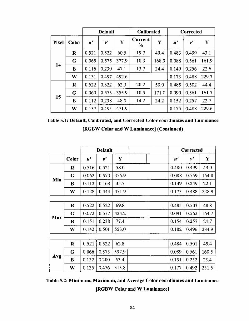
Pixel
14
15
Color
R
G
B
W
R
G
B
W
Default
u'
0.521
0.065
0.116
0.131
0.522
0.069
0.112
0.137
v'
0.522
0.575
0.230
0.497
0.522
0.573
0.238
0.495
Y
60.5
377.9
47.1
492.6
62.3
355.9
48.0
471.9
Calibrated
Current %
19.7
10.3
13.7
Y
49.4
168.3
24.4
20.2
10.5
14.2
50.0
171.0
24.2
Corrected
u'
0.483
0.088
0.149
0.173
0.485
0.090
0.152
0.175
v'
0.499
0.561
0.256
0.488
0.502
0.561
0.257
0.488
Y
43.1
161.9
22.6
229.7
44.4
161.7
22.7
229.6
Table 5.1: Default, Calibrated, and Corrected Color coordinates and Luminance
[RGBW Color and W Luminance] (Continued)
Min
Color
R
G
B
W
Default
u'
0.516
0.062
0.112
0.128
v'
0.521
0.573
0.163
0.444
Y
58.0
355.9
35.7
471.9
Corrected
u'
0.480
0.088
0.149
0.173
v'
0.499
0.559
0.249
0.488
Y
43.0
154.8
22.1
228.9
Max
R
G
B
W
0.522
0.072
0.151
0.142
0.522
0.577
0.238
0.501
69.8
424.2
77.4
553.0
0.485
0.091
0.154
0.182
0.503
0.562
0.257
0.496
48.8
164.7
24.7
234.9
Avg
R
G
B
W
0.521
0.066
0.132
0.135
0.522
0.575
0.200
0.476
62.8
392.9
53.4
513.8
0.484
0.089
0.151
0.177
0.501
0.561
0.252
0.492
45.4
160.5
23.4
231.5
Table 5.2: Minimum, Maximum, and Average Color coordinates and Luminance
[RGBW Color and W Luminance]
84
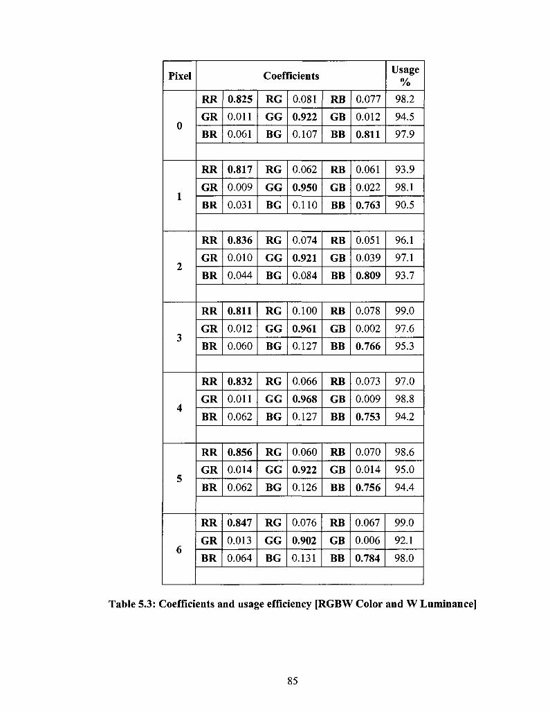
Pixel
0
1
2
3
4
5
6
Coefficients
RR
GR
BR
0.825
0.011
0.061
RG
GG
BG
0.081
0.922
0.107
RB
GB
BB
0.077
0.012
0.811
Usage %
98.2
94.5
97.9
RR
GR
BR
0.817
0.009
0.031
RG
GG
BG
0.062
0.950
0.110
RB
GB
BB
0.061
0.022
0.763
93.9
98.1
90.5
RR
GR
BR
0.836
0.010
0.044
RG
GG
BG
0.074
0.921
0.084
RB
GB
BB
0.051
0.039
0.809
96.1
97.1
93.7
RR
GR
BR
0.811
0.012
0.060
RG
GG
BG
0.100
0.961
0.127
RB
GB
BB
0.078
0.002
0.766
99.0
97.6
95.3
RR
GR
BR
0.832
0.011
0.062
RG
GG
BG
0.066
0.968
0.127
RB
GB
BB
0.073
0.009
0.753
97.0
98.8
94.2
RR
GR
BR
0.856
0.014
0.062
RG
GG
BG
0.060
0.922
0.126
RB
GB
BB
0.070
0.014
0.756
98.6
95.0
94.4
RR
GR
BR
0.847
0.013
0.064
RG
GG
BG
0.076
0.902
0.131
RB
GB
BB
0.067
0.006
0.784
99.0
92.1
98.0
Table 5.3: Coefficients and usage efficiency [RGBW Color and W Luminance]
85

Pixel
7
8
9
10
11
12
13
Coefficients
RR
GR
BR
0.876
0.014
0.058
RG
GG
BG
0.039
0.934
0.121
RB
GB
BB
0.072
0.016
0.754
Usage %
98.8
96.4
93.4
RR
GR
BR
0.868
0.014
0.062
RG
GG
BG
0.041
0.929
0.105
RB
GB
BB
0.064
0.017
0.788
97.4
96.0
95.5
RR
GR
BR
0.844
0.012
0.070
RG
GG
BG
0.066
0.904
0.133
RB
GB
BB
0.070
0.006
0.795
98.0
92.2
99.9
RR
GR
BR
0.821
0.012
0.063
RG
GG
BG
0.089
0.847
0.112
RB
GB
BB
0.061
0.013
0.794
97.0
87.3
96.8
RR
GR
BR
0.816
0.009
0.063
RG
GG
BG
0.075
0.922
0.148
RB
GB
BB
0.089
0.001
0.760
98.0
93.2
97.0
RR
GR
BR
0.856
0.016
0.055
RG
GG
BG
0.080
0.898
0.084
RB
GB
BB
0.044
0.032
0.750
98.0
94.6
88.9
RR
GR
BR
0.872
0.018
0.052
RG
GG
BG
0.037
0.925
0.095
RB
GB
BB
0.033
0.031
0.747
94.3
97.4
89.4
Table 5.3: Coefficients and usage efficiency
[RGBW Color and W Luminance] (Continued)
86
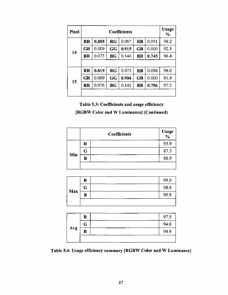
Pixel
14
15
Coefficients
RR
GR
BR
0.805
0.009
0.073
RG
GG
BG
0.087
0.915
0.146
RB
GB
BB
0.091
0.000
0.745
Usage %
98.2
92.5
96.4
RR
GR
BR
0.819
0.009
0.076
RG
GG
BG
0.073
0.904
0.141
RB
GB
BB
0.088
0.000
0.756
98.0
91.4
97.3
Table 5.3: Coefficients and usage efficiency
[RGBW Color and W Luminance] (Continued)
Min
Coefficients
R
G
B
Usage %
93.9
87.3
88.9
Max
R
G
B
99.0
98.8
99.9
Avg
R
G
B
97.5
94.6
94.9
Table 5.4: Usage efficiency summary [RGBW Color and W Luminance]
87

0.525
0.520
• i 0.505
Default.,
4* ^A
Corrected
0.475 0.480 0.485 0.480 0.495 0.500 0.505 0.510 0.515 0.520 0.525
0 1 2 3 4 5 6 7 8 9 10 11 12 13 14 15
Pixel No.
Figure 5.1: Red Corrected and Default Color & Luminance Parameters Chart
[RGBW Color and W luminance methodology]
0.575
0.570
•i
0.560
,-- ; ;x ) f «* * x " - - - . : x x x
X X . . -> — « ^ ^ ^ ^ * Default
Corrected _ _ ,'.»"""»
0.060 0.065 0.070
* — * T V
0.075 0.080 0.085 0.090
If
0.095
290
240
190 Corrected
140-1 1 1 1 H -I 1 1 1-0 1 2 3 4 5 6 7 8 9 10 11 12 13 14 1 !
Pixel No.
Figure 5.2: Green Corrected and Default Color & Luminance Parameters Chart
[RGBW Color and W luminance methodology]
88

0 1 2 3 4 5 6 7 8 9 10 11 12 13 14 15
Pixel No.
Figure 5.3: Blue Corrected and Default Color & Luminance Parameters Chart
[RGBW Color and W luminance methodology]
0.480
1» 0.470
0.460
/ x
/ * X
-^ x \
\ / ' T&K $ % *.
Corrected*—-'-.f* *c ''..-'
X X
— Defeult \ xx /
0.120 0.130 0.140 0.150 0.160 0.170 0.180 0.190
570
470
370
270
170
Default
Corrected
H 1 1 1 1 1 1 1 1-0 1 2 3 4 5 6 7 8 9 10 11 12 13 14 15;
PbdNo.
Figure 5.4: White Corrected and Default Color & Luminance Parameters Chart
[RGBW Color and W luminance methodology]
89
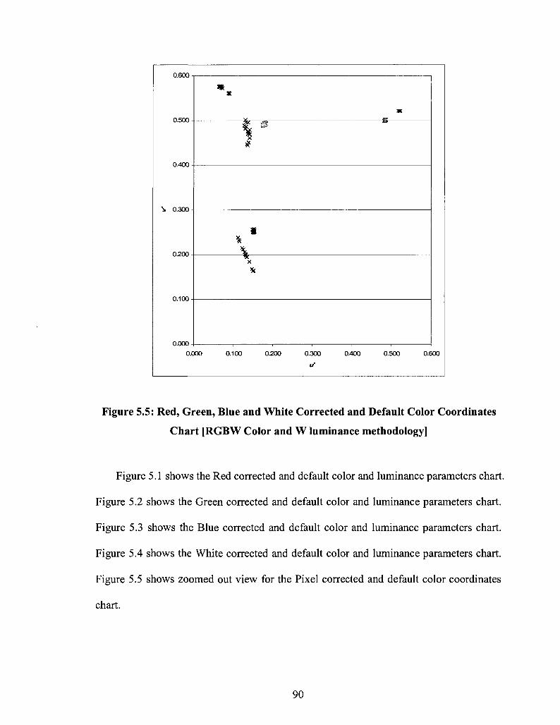
0.500-
0.200-
*
V -
£ m *
i
\ X
*
0.000 0.100 0.200 0.300
1/
0.400 0.500 0.600
Figure 5.5: Red, Green, Blue and White Corrected and Default Color Coordinates
Chart [RGBW Color and W luminance methodology]
Figure 5.1 shows the Red corrected and default color and luminance parameters chart.
Figure 5.2 shows the Green corrected and default color and luminance parameters chart.
Figure 5.3 shows the Blue corrected and default color and luminance parameters chart.
Figure 5.4 shows the White corrected and default color and luminance parameters chart.
Figure 5.5 shows zoomed out view for the Pixel corrected and default color coordinates
chart.
90
5.3 RGB Color and Luminance Experiment
For this experiment we had the following target color coordinates and luminance;
Red target color coordinates : u' = 0.480, v' = 0.500 target luminance: 43.
Green target color coordinates : u' = 0.090, v' = 0.560 target luminance: 160.
Blue target color coordinates : u' = 0.150, v' = 0.250 target luminance: 16.
Table 5.5 shows the results for the default, calibrated, and corrected data. Table 5.6
shows a summary for the minimum, maximum, and average values for each color. Table
5.7 shows the coefficients for each pixel and the used percentage from each calibrated
LED. Table 5.8 shows a summary for the maximum, minimum, and average usage
efficiency for the proposed methodology.
Figure 5.6 shows the corrected and default Red color and luminance parameters chart.
Figure 5.7 shows the corrected and default Green color and luminance parameters chart.
Figure 5.8 shows the corrected and default Blue color and luminance parameters chart.
Figure 5.9 shows the resulted corrected and default White color and luminance
parameters chart. Figure 5.10 shows zoomed out view for the Pixel corrected and default
color coordinates chart.
91
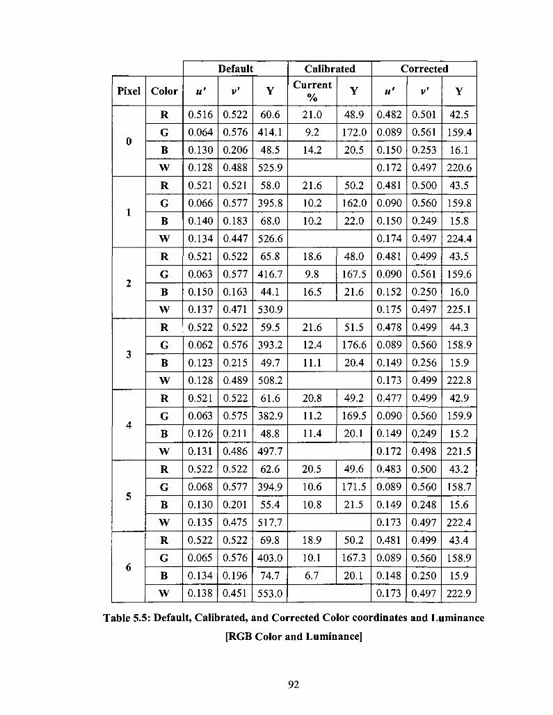
Pixel
0
1
2
3
4
5
6
Color
R
G
B
W
R
G
B
W
R
G
B
W
R
G
B
W
R
G
B
W
R
G
B
W
R
G
B
W
Default
« '
0.516
0.064
0.130
0.128
0.521
0.066
0.140
0.134
0.521
0.063
0.150
0.137
0.522
0.062
0.123
0.128
0.521
0.063
0.126
0.131
0.522
0.068
0.130
0.135
0.522
0.065
0.134
0.138
v'
0.522
0.576
0.206
0.488
0.521
0.577
0.183
0.447
0.522
0.577
0.163
0.471
0.522
0.576
0.215.
0.489
0.522
0.575
0.211
0.486
0.522
0.577
0.201
0.475
0.522
0.576
0.196
0.451
Y
60.6
414.1
48.5
525.9
58.0
395.8
68.0
526.6
65.8
416.7
44.1
530.9
59.5
393.2
49.7
508.2
61.6
382.9
48.8
497.7
62.6
394.9
55.4
517.7
69.8
403.0
74.7
553.0
Calibrated
Current %
21.0
9.2
14.2
Y
48.9
172.0
20.5
21.6
10.2
10.2
50.2
162.0
22.0
18.6
9.8
16.5
48.0
167.5
21.6
21.6
12.4
11.1
51.5
176.6
20.4
20.8
11.2
11.4
49.2
169.5
20.1
20.5
10.6
10.8
49.6
171.5
21.5
18.9
10.1
6.7
50.2
167.3
20.1
Corrected
u'
0.482
0.089
0.150
0.172
0.481
0.090
0.150
0.174
0.481
0.090
0.152
0.175
0.478
0.089
0.149
0.173
0.477
0.090
0.149
0.172
0.483
0.089
0.149
0.173
0.481
0.089
0.148
0.173
v'
0.501
0.561
0.253
0.497
0.500
0.560
0.249
0.497
0.499
0.561
0.250
0.497
0.499
0.560
0.256
0.499
0.499
0.560
0.249
0.498
0.500
0.560
0.248
0.497
0.499
0.560
0.250
0.497
Y
42.5
159.4
16.1
220.6
43.5
159.8
15.8
224.4
43.5
159.6
16.0
225.1
44.3
158.9
15.9
222.8
42.9
159.9
15.2
221.5
43.2
158.7
15.6
222.4
43.4
158.9
15.9
222.9
Table 5.5: Default, Calibrated, and Corrected Color coordinates and Luminance
[RGB Color and Luminance]
92

Pixel
7
8
9
10
11
12
13
Color
R
G
B
W
R
G
B
W
R
G
B
W
R
G
B
W
R
G
B
W
R
G
B
W
R
G
B
W
Default
u'
0.521
0.071
0.132
0.138
0.522
0.072
0.132
0.142
0.520
0.067
0.135
0.135
0.521
0.064
0.131
0.130
0.521
0.066
0.115
0.130
0.521
0.065
0.148
0.140
0.519
0.068
0.151
0.141
v'
0.521
0.576
0.198
0.475
0.522
0.573
0.198
0.469
0.522
0.574
0.195
0.444
0.522
0.575
0.200
0.482
0.521
0.576
0.232
0.501
0.522
0.574
0.168
0.461
0.522
0.577
0.164
0.479
Y
64.9
397.9
54.7
522.1
63.6
367.4
53.6
489.1
62.3
395.1
77.4
540.6
64.1
424.2
52.5
544.7
63.2
405.0
48.2
521.1
64.8
387.1
48.5
505.1
61.1
374.5
35.7
474.4
Calibrated
Current %
19.1
9.3
10.1
Y
50.7
166.7
20.3
20.0
11.1
9.5
50.9
170.6
19.0
20.0
8.2
6.1
51.0
166.6
19.7
20.2
8.2
10.3
50.0
173.8
19.4
19.4
9.0
11.1
49.4
169.3
20.8
20.2
9.2
9.2
50.4
168.0
18.7
20.5
10.3
17.2
49.6
166.2
22.1
Corrected
u'
0.480
0.090
0.150
0.173
0.479
0.089
0.149
0.173
0.478
0.090
0.149
0.174
0.480
0.089
0.149
0.173
0.477
0.089
0.150
0.173
0.480
0.089
0.148
0.173
0.478
0.090
0.149
0.171
v'
0.499
0.560
0.252
0.497
0.499
0.560
0.250
0.497
0.499
0.560
0.251
0.497
0.499
0.561
0.251
0.497
0.499
0.561
0.256
0.497
0.499
0.560
0.252
0.497
0.498
0.559
0.256
0.503
Y
43.5
159.7
16.1
222.6
43.7
159.1
15.9
223.0
44.0
159.8
16.2
224.0
43.7
159.0
16.2
222.7
44.1
159.2
16.7
223.1
43.5
159.1
16.3
223.3
43.4
160.0
16.5
222.6
Table 5.5: Default, Calibrated, and Corrected Color coordinates and Luminance
[RGB Color and Luminance] (Continued)
93

Pixel
14
15
Color
R
G
B
W
R
G
B
W
Default
« '
0.521
0.065
0.116
0.131
0.522
0.069
0.112
0.137
v'
0.522
0.575
0.230
0.497
0.522
0.573
0.238
0.495
Y
60.5
377.9
47.1
492.6
62.3
355.9
48.0
471.9
Calibrated
Current %
20.0
10.3
9.9
Y
51.6
167.2
19.3
19.9
10.9
11.7
51.0
170.0
20.0
Corrected
**'
0.483
0.089
0.152
0.174
0.479
0.090
0.152
0.173
v'
0.500
0.561
0.248
0.497
0.500
0.560
0.256
0.497
Y
43.1
159.1
15.8
222.6
43.7
159.9
17.0
221.6
Table 5.5: Default, Calibrated, and Corrected Color coordinates and Luminance
[RGB Color and Luminance] (Continued)
Min
Color
R
G
B
W
Default
u'
0.516
0.062
0.112
0.128
v'
0.521
0.573
0.163
0.444
Y
58.0
355.9
35.7
471.9
Corrected
u'
0.477
0.089
0.148
0.171
v'
0.498
0.559
0.248
0.497
Y
42.5
158.7
15.2
220.6
Max
R
G
B
W
0.522
0.072
0.151
0.142
0.522
0.577
0.238
0.501
69.8
424.2
77.4
553.0
0.483
0.090
0.152
0.175
0.501
0.561
0.256
0.503
44.3
160.0
17.0
225.1
Avg
R
G
B
W
0.521
0.066
0.132
0.135
0.522
0.575
0.200
0.476
62.8
392.9
53.4
513.8
0.480
0.089
0.150
0.173
0.499
0.560
0.252
0.498
43.5
159.4
16.1
222.8
Table 5.6: Minimum, Maximum, and Average Color coordinates and Luminance
[RGB Color and Luminance]
94

Pixel
0
1
2
3
4
5
6
Coefficients
RR
GR
BR
0.846
0.009
0.079
RG
GG
BG
0.085
0.838
0.159
RB
GB
BB
0.015
0.005
0.759
Usage %
94.5
85.2
99.7
RR
GR
BR
0.818
0.015
0.067
RG
GG
BG
0.076
0.945
0.138
RB
GB
BB
0.015
0.019
0.625
90.9
97.9
83.0
RR
GR
BR
0.854
0.017
0.051
RG
GG
BG
0.092
0.915
0.103
RB
GB
BB
0.015
0.045
0.474
96.1
97.7
62.8
RR
GR
BR
0.806
0.011
0.074
RG
GG
BG
0.117
0.809
0.139
RB
GB
BB
0.015
0.001
0.767
93.9
82.1
98.0
RR
GR
BR
0.818
0.013
0.073
RG
GG
BG
0.108
0.949
0.142
RB
GB
BB
0.015
0.003
0.765
94.1
96.5
98.0
RR
GR
BR
0.833
0.013
0.069
RG
GG
BG
0.079
0.863
0.135
RB
GB
BB
0.015
0.013
0.667
92.7
88.8
87.1
RR
GR
BR
0.820
0.012
0.077
RG
GG
BG
0.083
0.816
0.149
RB
GB
BB
0.015
0.011
0.724
91.8
83.9
95.0
Table 5.7: Coefficients and Usage efficiency [RGB Color and Luminance]
95

Pixel
7
8
9
10
11
12
13
Coefficients
RR
GR
BR
0.812
0.013
0.078
RG
GG
BG
0.085
0.915
0.155
RB
GB
BB
0.015
0.006
0.754
Usage %
91.2
93.5
98.6
RR
GR
BR
0.806
0.014
0.080
RG
GG
BG
0.080
0.897
0.155
RB
GB
BB
0.015
0.014
0.751
90.2
92.5
98.6
RR
GR
BR
0.805
0.015
0.077
RG
GG
BG
0.048
0.945
0.151
RB
GB
BB
0.015
0.015
0.722
86.8
97.5
95.0
RR
GR
BR
0.821
0.015
0.078
RG
GG
BG
0.052
0.945
0.130
RB
GB
BB
0.015
0.015
0.732
88.8
97.5
94.0
RR
GR
BR
0.835
0.013
0.077
RG
GG
BG
0.084
0.914
0.138
RB
GB
BB
0.015
0.007
0.726
93.4
93.5
94.1
RR
GR
BR
0.815
0.013
0.081
RG
GG
BG
0.117
0.856
0.137
RB
GB
BB
0.015
0.013
0.760
94.7
88.3
97.8
RR
GR
BR
0.826
0.010
0.083
RG
GG
BG
0.088
0.913
0.170
RB
GB
BB
0.015
0.001
0.727
92.9
92.4
98.0
Table 5.7: Coefficients and Usage efficiency
[RGB Color and Luminance] (Continued)
96
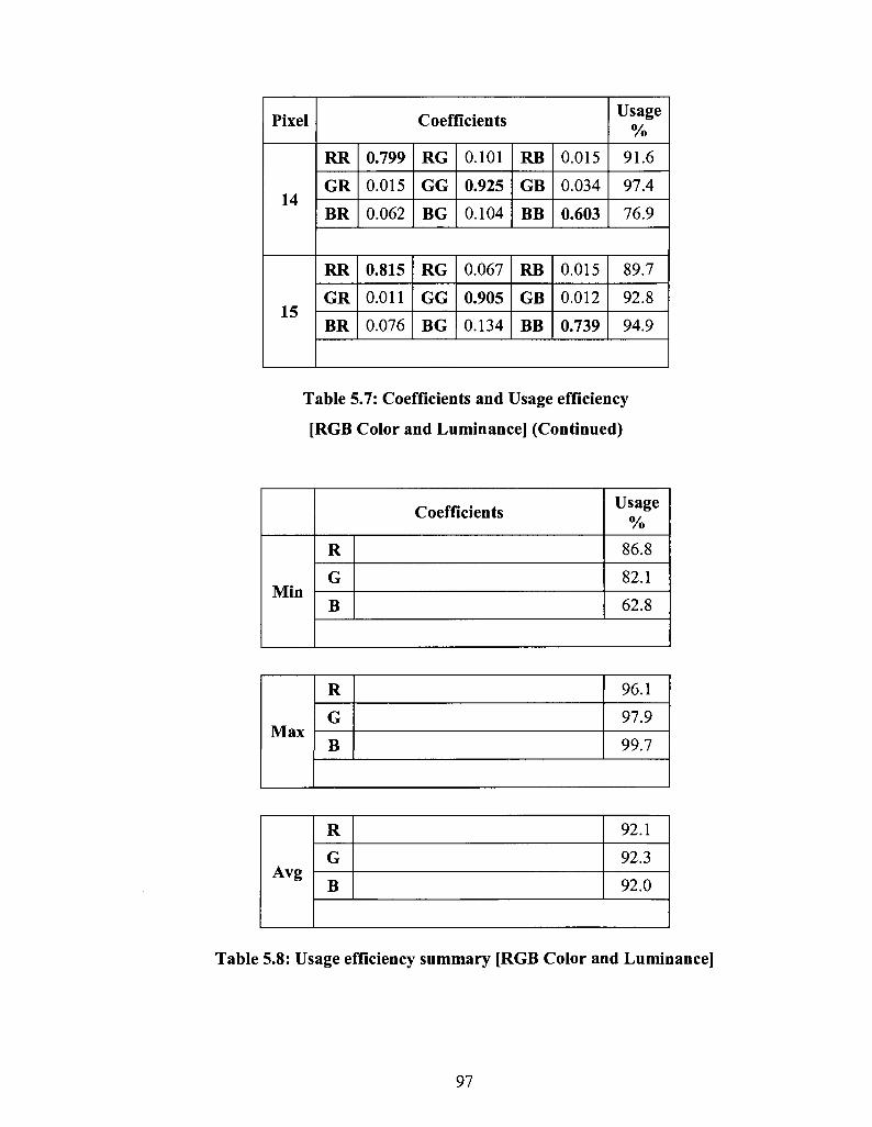
Pixel
14
15
Coefficients
RR
GR
BR
0.799
0.015
0.062
RG
GG
BG
0.101
0.925
0.104
RB
GB
BB
0.015
0.034
0.603
Usage %
91.6
97.4
76.9
RR
GR
BR
0.815
0.011
0.076
RG
GG
BG
0.067
0.905
0.134
RB
GB
BB
0.015
0.012
0.739
89.7
92.8
94.9
Table 5.7: Coefficients and Usage efficiency
[RGB Color and Luminance] (Continued)
Min
Coefficients
R
G
B
Usage %
86.8
82.1
62.8
Max
R
G
B
96.1
97.9
99.7
Avg
R
G
B
92.1
92.3
92.0
Table 5.8: Usage efficiency summary [RGB Color and Luminance]
97
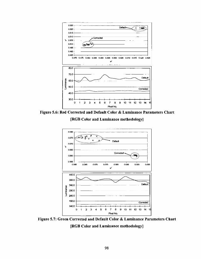
Default*
Cotrected
W
0.470 0.475 0.480 0.485 0.480 0.495 0.500 0.505 0.510 0.515 0.520 0.525
Figure 5.6: Red Corrected and Default Color & Luminance Parameters Chart
[RGB Color and Luminance methodology]
0.575
^
0.555
. - - ; ; * # « * * " • • • « .
; " x x X X..-
0.060 0.065 0.070
* Default
Corrected » ^ ^
0.075 0.080 0.085
u'
•' W \ * /
0.090 0.095
390.0
140.0
\ ^ / - \ / ~ \ ^ ~"" \^ /^ '
Default
Corrected
1 1 1 1 1 1 1 1 1 1 1 1 1 1
0 1 2 3 4 5 6 7 8 9 10 11 12 13 14 i q
Pixel No.
Figure 5.7: Green Corrected and Default Color & Luminance Parameters Chart
[RGB Color and Luminance methodology]
98

0.300 n
0.140
Default *
Ccrrected*
"'--
~\*Rf &J
• - . .
X XX" - * ,
70.0
50.0
0.100 0.110 0.120 0.130 0.140 0.150 0.160
Pixel No.
Figure 5.8: Blue Corrected and Default Color & Luminance Parameters Chart
[RGB Color and Luminance methodology]
V 0.470
0.430 0.120
/ x
r \
X
'••-y - / -
Corrected "
— Defeult
"••,.xx /
570
470
370
270
170
0.130 0.140 0.150 0.160 0.170 0.180
Default
Corrected
H 1 1 1 1 1 1 h H 1 1 h
0 1 2 3 4 5 6 7 8 9 10 11 12 13 14 1£| Pi)el No.
Figure 5.9: White Corrected and Default Color & Luminance Parameters Chart
[RGB Color and Luminance methodology]
99

Figure 5.10: Red, Green, Blue and White Corrected and Default Color Coordinates
Chart [RGB Color and Luminance methodology]
100
5.4 RGB Luminance Experiment
For this experiment we had the following target luminance;
Red target luminance : 45 nits
Green target luminance : 160 nits
Blue target luminance : 20 nits
Table 5.9 shows the results for the default and calibrated data. Table 5.10 shows a
summary for the minimum, maximum, and average values for each color. Since this
methodology doesn't correct the colors, the coefficients will be as the following for all
the pixels:
KRR = 1 KRQ = 0 KRB - 0
KGR = 0 KQG = 1 KGB
= 0
KBR = 0 KBG = 0 KBB
= 1
Figure 5.11 shows the calibrated and default Red color and luminance parameters
chart. Figure 5.12 shows the calibrated and default Green color and luminance parameters
chart. Figure 5.13 shows the calibrated and default Blue color and luminance parameters
chart. Figure 5.14 shows the resulted calibrated and default White color and luminance
parameters chart. Figure 5.15 shows zoomed out view for the Pixel calibrated and default
color coordinates chart.
101

Pixel
0
1
2
3
4
5
6
Color
R
G
B
W
R
G
B
W
R
G
B
W
R
G
B
W
R
G
B
W
R
G
B
W
R
G
B
W
Default « '
0.516
0.064
0.130
0.128
0.521
0.066
0.140
0.134
0.521
0.063
0.150
0.137
0.522
0.062
0.123
0.128
0.521
0.063
0.126
0.131
0.522
0.068
0.130
0.135
0.522
0.065
0.134
0.138
v'
0.522
0.576
0.206
0.488
0.521
0.577
0.183
0.447
0.522
0.577
0.163
0.471
0.522
0.576
0.215
0.489
0.522
0.575
0.211
0.486
0.522
0.577
0.201
0.475
0.522
0.576
0.196
0.451
Y
60.6
414.1
48.5
525.9
58.0
395.8
68.0
526.6
65.8
416.7
44.1
530.9
59.5
393.2
49.7
508.2
61.6
382.9
48.8
497.7
62.6
394.9
55.4
517.7
69.8
403.0
74.7
553.0
Calibrated
u'
0.519
0.077
0.121
0.170
0.522
0.076
0.126
0.172
0.522
0.075
0.145
0.179
0.522
0.072
0.115
0.173
0.522
0.071
0.117
0.168
0.522
0.076
0.124
0.173
0.522
0.078
0.123
0.181
v'
0.522
0.580
0.220
0.497
0.522
0.580
0.209
0.488
0.522
0.580
0.170
0.466
0.522
0.579
0.230
0.495
0.522
0.579
0.224
0.500
0.522
0.579
0.211
0.489
0.522
0.580
0.214
0.489
Y
44.1
157.6
20.8
223.2
46.1
162.1
21.0
230.9
43.9
157.2
19.7
224.0
44.5
158.4
19.7
223.3
44.9
159.2
19.1
225.5
45.0
159.6
20.6
226.5
45.6
158.6
19.5
224.1
Table 5.9: Default and Calibrated Color Coordinates and Luminance
[RGB Luminance]
102
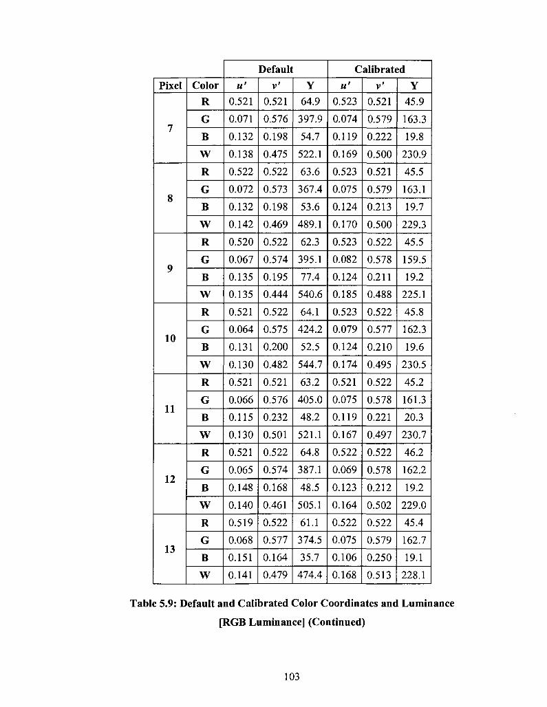
Pixel
7
8
9
10
11
12
13
Color
R
G
B
W
R
G
B
W
R
G
B
W
R
G
B
W
R
G
B
W
R
G
B
W
R
G
B
W
Default
u'
0.521
0.071
0.132
0.138
0.522
0.072
0.132
0.142
0.520
0.067
0.135
0.135
0.521
0.064
0.131
0.130
0.521
0.066
0.115
0.130
0.521
0.065
0.148
0.140
0.519
0.068
0.151
0.141
v'
0.521
0.576
0.198
0.475
0.522
0.573
0.198
0.469
0.522
0.574
0.195
0.444
0.522
0.575
0.200
0.482
0.521
0.576
0.232
0.501
0.522
0.574
0.168
0.461
0.522
0.577
0.164
0.479
Y
64.9
397.9
54.7
522.1
63.6
367.4
53.6
489.1
62.3
395.1
77.4
540.6
64.1
424.2
52.5
544.7
63.2
405.0
48.2
521.1
64.8
387.1
48.5
505.1
61.1
374.5
35.7
474.4
Calibrated
u'
0.523
0.074
0.119
0.169
0.523
0.075
0.124
0.170
0.523
0.082
0.124
0.185
0.523
0.079
0.124
0.174
0.521
0.075
0.119
0.167
0.522
0.069
0.123
0.164
0.522
0.075
0.106
0.168
v'
0.521
0.579
0.222
0.500
0.521
0.579
0.213
0.500
0.522
0.578
0.211
0.488
0.522
0.577
0.210
0.495
0.522
0.578
0.221
0.497
0.522
0.578
0.212
0.502
0.522
0.579
0.250
0.513
Y
45.9
163.3
19.8
230.9
45.5
163.1
19.7
229.3
45.5
159.5
19.2
225.1
45.8
162.3
19.6
230.5
45.2
161.3
20.3
230.7
46.2
162.2
19.2
229.0
45.4
162.7
19.1
228.1
Table 5.9: Default and Calibrated Color Coordinates and Luminance
[RGB Luminance] (Continued)
103

Pixel
14
15
Color
R
G
B
W
R
G
B
W
Default
« '
0.521
0.065
0.116
0.131
0.522
0.069
0.112
0.137
v'
0.522
0.575
0.230
0.497
0.522
0.573
0.238
0.495
Y
60.5
377.9
47.1
492.6
62.3
355.9
48.0
471.9
Calibrated
u'
0.522
0.070
0.138
0.171
0.519
0.079
0.125
0.178
v'
0.522
0.577
0.184
0.483
0.522
0.577
0.212
0.492
Y
46.1
162.6
19.5
231.9
45.7
160.6
19.8
228.3
Table 5.9: Default and Calibrated Color Coordinates and Luminance
[RGB Luminance] (Continued)
Min
Color
R
G
B
W
Default
« '
0.516
0.062
0.112
0.128
v'
0.521
0.573
0.163
0.444
Y
58.0
355.9
35.7
471.9
Calibrated
« '
0.519
0.069
0.106
0.164
v'
0.521
0.577
0.170
0.466
Y
43.9
157.2
19.1
223.2
Max
R
G
B
W
0.522
0.072
0.151
0.142
0.522
0.577
0.238
0.501
69.8
424.2
77.4
553.0
0.523
0.082
0.145
0.185
0.522
0.580
0.250
0.513
46.2
163.3
21.0
231.9
Avg
R
G
B
W
0.521
0.066
0.132
0.135
0.522
0.575
0.200
0.476
62.8
392.9
53.4
513.8
0.522
0.075
0.123
0.173
0.522
0.579
0.213
0.493
45.3
160.6
19.8
227.6
Table 5.10: Minimum, Maximum, and Average Color Coordinates and Luminance
[RGB Luminance]
104

- ___
0.522-
0.521
X
X
* X J ' . ^ H f T*
0.515 0.516 0.517 0.518 0.519 u
0.520
X Calibrated
X Default
0.521 0.522 0.523 0.524
Figure 5.11: Red Calibrated and Default Color & Luminance Parameters Chart
[RGB Luminance methodology]
_ ___
0.580-
0.575
O.C 160
x x * x x x „
X
0.065
X X
x x X X
X
x x
0.070 u'
X
0.075
X X
X
* x
X Calibrated
X Default
0.080 O.C 85
Figure 5.12: Green Calibrated and Default Color & Luminance Parameters Chart
[RGB Luminance methodology]
105

0.260
0.240
0.220
V 0.200
0.180
0.160
0.140 0.100 0.110 0.120 0.130 0.140 0.150 0.1601
X
* % x %
X
X X
Calibrate X
DefaultX * X
X X
8 9 10 11 12 13 14 19
Figure 5.13: Blue Calibrated and Default Color & Luminance Parameters Chart
[RGB Luminance methodology]
0.520
0.510
0.500
0.490
0.480
0.470
0.460
0.450
0.440
0.430
sc
X
x x
X * x scr X
* X
X X
X
*x X Calibrated
X Default
0.120 0.130 0.140 0.150 0.160 0.170 0.180 0.190
280
230
180
ian-
S \ y' - - .
"— ^ \ _ / ~ \ Default
=- = ^ = = =
1 1 1 1 1—
' —
1 1 1 1 1 1
Corrected
1 1 1
0 1 2 3 4 5 6 7 8 9 10 11 12 13 14 1!
Figure 5.14: White Calibrated and Default Color & Luminance Parameters Chart
[RGB Luminance methodology]
106

0.600
0.500
0.400
^ 0.300
0.200
0.100
0.000
3jfR
#
\
0.000 0.100 0.200 0.300
1/
0.400 0.500 0.600
Figure 5.15: Red, Green, Blue and White Calibrated and Default Color Coordinates
Chart [RGB Luminance methodology]
107
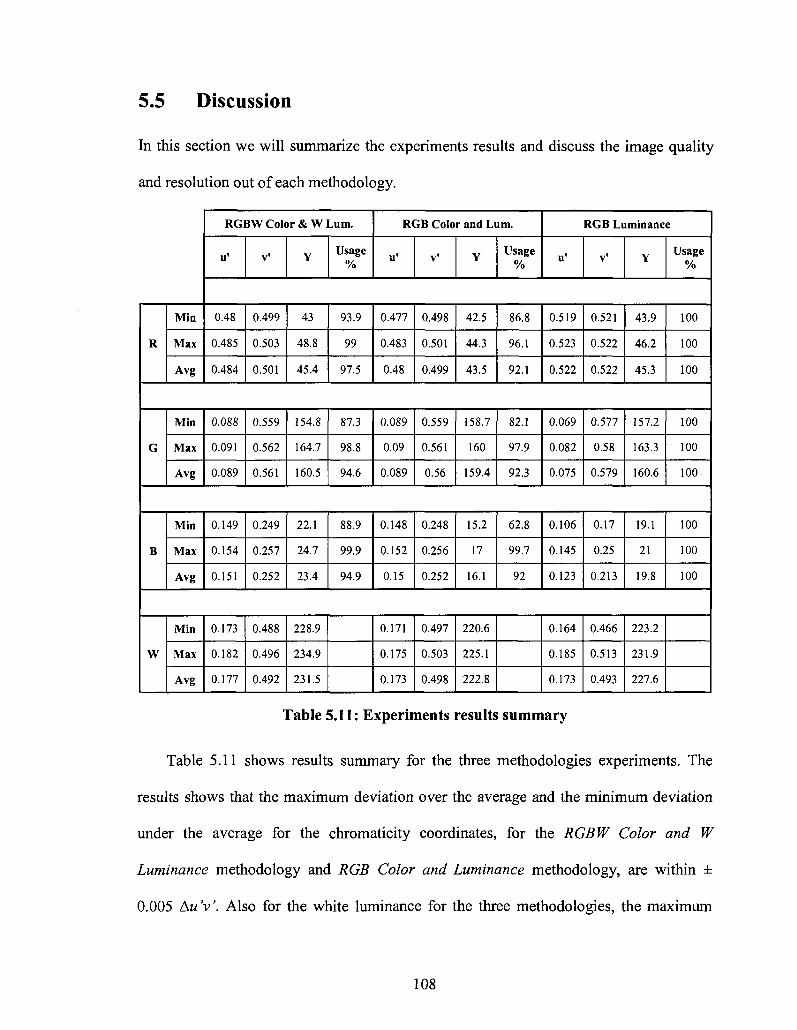
5.5 Discussion
In this section we will summarize the experiments results and discuss the image quality
and resolution out of each methodology.
R
Min
Max
Avg
RGBW Color & W Lum.
u' v' Y Usage
%
RGB Color and Lum.
u' V' Y Usage %
RGB Luminance
u' v' Y Usage
%
0.48
0.485
0.484
0.499
0.503
0.501
43
48.8
45.4
93.9
99
97.5
0.477
0.483
0.48
0.498
0.501
0.499
42.5
44.3
43.5
86.8
96.1
92.1
0.519
0.523
0.522
0.521
0.522
0.522
43.9
46.2
45.3
100
100
100
G
Min
Max
Avg
0.088
0.091
0.089
0.559
0.562
0.561
154.8
164.7
160.5
87.3
98.8
94.6
0.089
0.09
0.089
0.559
0.561
0.56
158.7
160
159.4
82.1
97.9
92.3
0.069
0.082
0.075
0.577
0.58
0.579
157.2
163.3
160.6
100
100
100
B
Min
Max
Avg
0.149
0.154
0.151
0.249
0.257
0.252
22.1
24.7
23.4
88.9
99.9
94.9
0.148
0.152
0.15
0.248
0.256
0.252
15.2
17
16.1
62.8
99.7
92
0.106
0.145
0.123
0.17
0.25
0.213
19.1
21
19.8
100
100
100
W
Min
Max
Avg
0.173
0.182
0.177
0.488
0.496
0.492
228.9
234.9
231.5
0.171
0.175
0.173
0.497
0.503
0.498
220.6
225.1
222.8
0.164
0.185
0.173
0.466
0.513
0.493
223.2
231.9
227.6
Table 5.11: Experiments results summary
Table 5.11 shows results summary for the three methodologies experiments. The
results shows that the maximum deviation over the average and the minimum deviation
under the average for the chromaticity coordinates, for the RGBW Color and W
Luminance methodology and RGB Color and Luminance methodology, are within ±
0.005 AuV. Also for the white luminance for the three methodologies, the maximum
108

deviation over the average and the minimum deviation under the average are within ± 3%.
R
Min
Max
Avg
Default
u' V' Y Usage %
0.516
0.522
0.521
0.521
0.522
0.522
58.0
69.8
62.8
100
100
100
G
Min
Max
Avg
0.062
0.072
0.066
0.573
0.577
0.575
355.9
424.2
392.9
100
100
100
B
Min
Max
Avg
0.112
0.151
0.132
0.163
0.238
0.200
35.7
77.4
53.4
100
100
100
W
Min
Max
Avg
0.128
0.142
0.135
0.444
0.501
0.476
471.9
553.0
513.8
Table 5.12: Default results summary
Table 5.12 shows the default color coordinates and luminances for the LED colors
before the correction and the calibration. The Red and Green LEDs do have small color
coordinates deviations under and over the average; on the other hand, they have a large
deviation in the luminances. The Blue and the resulted White have a large deviation in
both color coordinates and luminances.
As for the image quality, the RGBW Color and WLuminance methodology and RGB
Color and Luminance methodology experiments results show how all the deviations in
the color and luminance were significantly reduced, which leads for a high image quality.
109
The RGB Luminance methodology reduced the deviation in the luminance significantly,
which leads to a less color perception differences.
As for the image resolution, the RGB Luminance methodology keeps the maximum
resolution that can be provided by the LED Screen. The RGBW Color and WLuminance
methodology and RGB Color and Luminance methodology provide less resolution
associate with a high image quality. The experimental results show how the RGBW Color
and WLuminance methodology can provide a higher resolution than the RGB Color and
Luminance methodology. On the other hand, the RGB Color and Luminance
methodology provides a faster correction process than the RGBW Color and W
Luminance methodology.
110
CHAPTER 6
Conclusion and Future Work
6.1 Conclusion
In this thesis, a novel technique for color and luminance correction and calibration
for LED Video screens was presented. The proposed method used the CIE color system
for measuring and calculating the color coordinates and Luminance. A new algorithm
was developed to calculate the color mixture components, based on the CIE system, to
calibrate and correct the LED pixels in the LED screens.
The proposed technique was an integrated hardware and software solution where it
uses robotic spectrometer head and Windows based graphical user interface (GUI)
application software. The software was developed using Visual Basic .net (VB.net). The
proposed technique was implemented, tested, and integrated in collaboration with LSI
SACO technologies.
The root cause of the color and luminance non-uniformity problem in the LED
screens along with the available solutions in the market were presented and discussed.
The Image quality and resolution along with the cost was the main target of the proposed
correction system as these are the main keys for a cost-effective and high quality product.
The system can run different methodologies, which are based on the developed algorithm,
to calibrate and correct the LED screen. The user has the choice to select the proper
111
methodology according to his need. The experiments show the results for three different
methodologies along with the image quality and resolution efficiency out of each of them.
One methodology was developed for LED lighting products correction and calibration,
although the other methodologies still can be applied for LED lighting products as well.
6.2 Future Work
The proposed system in this thesis provides accurate correction coefficients with very
small pixel-to-pixel color and luminance differences, ± 0.03% brightness and ± 0.005
AwV, where it is needed to enhance the algorithm further more to reduce these
differences. In addition, as a future work, from the practical point of view, the current
system measures, calibrates and corrects one single pixel at the time, so it is valuable to
add another spectrometer head to speed up the calibration process. Other things can be
considered to enhance the system measurement and calibration speed, by having larger
solid core fiber cable and extra optics (as lenses) to amplify the input light to the
spectrometer to have more accurate light readings.
Finally, we believe this thesis project is an important milestone towards producing a
cost-effective and high quality and resolution LED video screens. Therefore, it is
important to develop the system further more to make it a commercial viable device.
112

Bibliography
[1] Muthu, S., Schuurmans, F.J., Pashley, M.D. "Red, green, and blue LED based
white light generation: issues and control" Industry Applications Conference,
Volume 1, Issue Pages: 327 - 333, 2002.
[2] S. Muthu, FJ.P. Schuurmans, M.D. Pashley, "Red, green, and blue LEDs for
white light illumination," IEEE Journal on Selected Topics in Quantum
Electronics, vol. 8, no. 2, March/April 2002, pp. 333-338.
[3] S. Muthu, FJ.P. Schuurmans, M.D. Pashley, "Red, green, and blue LED based
white light generation: Issues and control," Conference Record of the 2002 IEEE
Industry Applications Conference, 37th IAS Annual Meeting, Pittsburgh, PA,
USA, 13-18 Oct. 2002, vol. 1, 2002, pp. 327- 333.
[4] S. Muthu, J. Gaines, "Red, green, and blue LED-based white light source:
Implementation challenges and control design," Conference Record of the 2003
IEEE Industry Applications Conference, 38th IAS Annual Meeting, Salt Lake
City, UT, USA, 12-16 Oct. 2003, vol. 1, 2003, pp. 515-522.
[5] A. Zukauskas, R. Vaicekauskas, F. Ivanauskas, G. Kurilcik, Z. Bliznikas, K.
Breive, J. Krupic, A. Rupsys, A. Novickovas, P. Vitta, A. Navickas, V.
Raskauskas, M.S. Shur, R. Gaska, "Quadrichromatic white solid state lamp with
digital feedback," Proceedings of the SPIE - The International Society for Optical
Engineering, Third International Conference on Solid State Lighting, San Diego,
113
CA, USA, 5-7 Aug. 2003, vol. 5187, no. 1, Jan. 2004, pp. 185-198.
[6] A. Perduijn, S. de Krijger, J. Claessens, N. Kaito, T. Yagi, S.T. Hsu, M.
Sakakibara, T. Ito, S. Okada, "Light output feedback solution for RGB LED
backlight applications," SID 03 DIGEST, 2003, pp. 1254-1257.
[7] P. Deurenberg, C. Hoelen, J. van Meurs, J. Ansems, "Achieving color point
stability in RGB multi-chip LED modules using various color control loops,"
Proceedings of the SPIE - The International Society for Optical Engineering, Fifth
International Conference on Solid State Lighting, San Diego, CA, USA, 31 Jul. -4
Aug. 2005, vol. 5941, Sep. 2005, pp. 63-74.
[8] I.E. Ashdown, "Neural networks for LED color control," Proceedings of the SPIE
- The International Society for Optical Engineering, Third International
Conference on Solid State Lighting, San Diego, CA, USA, 5-7 Aug. 2003, vol.
5187, no. 1, Jan. 2004, pp. 215-226.
[9] S.Muthu, F. Schuurmans, and M. Pashley, "Red, Green and Blue LEDs for white
light illumination", IEEE journal on selected topics in quatum electronics, pp. Vol.
8, No. 2, March/April 2002.
[10] Nichia Corporation, Display SMD LED, http://www.nichia.com/product/led-
display-smt.html, May 2009
[11] Radiant Imaging, LED Screen Correction System,
http://www.radiantimaging.com/?q=products/pm_led, May 2009
114
[12] LSI SACO Technologies, LED Screens, http://www.smartvision.com, May 2009
[13] Xichao Mo; Yuanyue Zhang, "Consecutive PWM driving video LED display
system", IEEE International Symposium on Circuits and Systems, pp. Vol. 2, No.
2, Page(s):1437 - 1439, June 1997.
[14] Young-Chang Chang; Reid, J.F, "RGB calibration for color image analysis in
machine vision", IEEE Transactions on Image Processing, pp. Vol. 5, No. 10,
Page(s):1414- 1422, Oct. 1996.
[15] CIE, 2007. CIE 127:2007, "Measurement of LEDs", 2nd edition, 2007.
[16] CIE, Color System, http://www.cie.co.at
[ 17] Shubert E. Light Emitting Diodes. Cambridge University Press; 2003
[18] Philips Lumileds Lighting Company, LED Lighting Products,
http://www.lumileds.com, May 2009
[19] Texas Instruments Corporation, LED Driver,
http://focus.ti.com/docs/prod/folders/print/tlc5925.html, May 2009
[20] Silicon Touch Technology Inc., http://www.siti.com.tw/product/product6_en.html,
May 2009
[21] Hunt, Robert W. G., Measuring Colour. Chichester: Ellis Horwood Ltd, 1987.
[22] CIE/IEC, 1987, CIE 17.4:1987, "International Lighting Vocabulary". 1987.
115
[23] Deane B. Judd and Gunter Wyszecki, Color in Business, Science and Industry
(3rd edition). John Wiley, 1975. pp. 296.
[24] Daniel Malacara, Color Vision and Colorimetry: Theory and Applications. SPUE
Press, 2002
[25] Fred W. Billmeyer, Jr. and Max Saltzman, Principles of Color Technology (2nd
edition). John Wiley, 1981. pp. 42, pp. 58.
[26]- Adrian Ford and Alan Roberts, http://www.poynton.com/PDFs/coloureq.pdf, May
2009
[27] Williamson, Samuel J., Light and Color in nature and art, John Wiley, 1983.
[28] Mercier, G.; Ross, J.; Ginobbi, P.; Venkat, R.; "A Robotic Spectrometer System
for LED Display Measurements", IEEE transaction on System Engineering, pp.,
Pages: 412 - 417, Aug 2008.
[29] B. Ackermann, V. Schulz, C. Martiny, A. Hilgers, "Control of LEDs", IEEE
transaction on Digital Object Identifier, pp., Pages: 2608 - 2615, Oct 2006.
[30] Shlayan, N.; Venkat, R.; Ginobbi, P.; Mercier, G.; "A Novel RGBW Pixel for
LED Displays", IEEE transaction on Digital Object Identifier, pp., Pages: 407 -
411, Aug 2008.
116
[31] Lucchese, L.; Mitra, S.K.; "A new class of chromatic filters for color image
processing. Theory and applications", IEEE transaction on Digital Object
Identifier, pp., Pages: 534 - 548, April 2004.
[32] D. L. MacAdam; "Visual Sensitivities to Color Differences in Daylight", Journal
Optical Society of America, pp., Vol. 32, Pages: 247-274, May 1942.
[33] D. L. MacAdam; "Specification of Small Chromaticity Differences", Journal
Optical Society of America, pp., Vol. 33, Pages: 18-26, Jan 1943.
[34] Photon Control, Spectrometers, http://www.photon-control.com, May 2009
[35] Janome Robots, 3D Robots, http://www.janomeie.com, May 2009
[36] Alex Byrne, David R. Hilbert, "Readings on Color: The philosophy of color", 2nd
edition, MIT Press, 1997, Pages. 194-198.
117

Appendix A
CIE 1931 color matching functions;
Measurements table of (5 nm intervals)
X, nm
380
385
390
395
400
405
410
415
420
425
430
435
440
445
450
455
460
465
470
475
480
485
F(A)
0.001368
0.002236
0.004243
0.007650
0.014310
0.023190
0.043510
0.077630
0.134380
0.214770
0.283900
0.328500
0.348280
0.348060
0.336200
0.318700
0.290800
0.251100
0.195360
0.142100
0.095640
0.057950
7(A)
0.000039
0.000064
0.000120
0.000217
0.000396
0.000640
0.001210
0.002180
0.004000
0.007300
0.011600
0.016840
0.023000
0.029800
0.038000
0.048000
0.060000
0.073900
0.090980
0.112600
0.139020
0.169300
z(A)
0.006450
0.010550
0.020050
0.036210
0.067850
0.110200
0.207400
0.371300
0.645600
1.039050
1.385600
1.622960
1.747060
1.782600
1.772110
1.744100
1.669200
1.528100
1.287640
1.041900
0.812950
0.616200
118
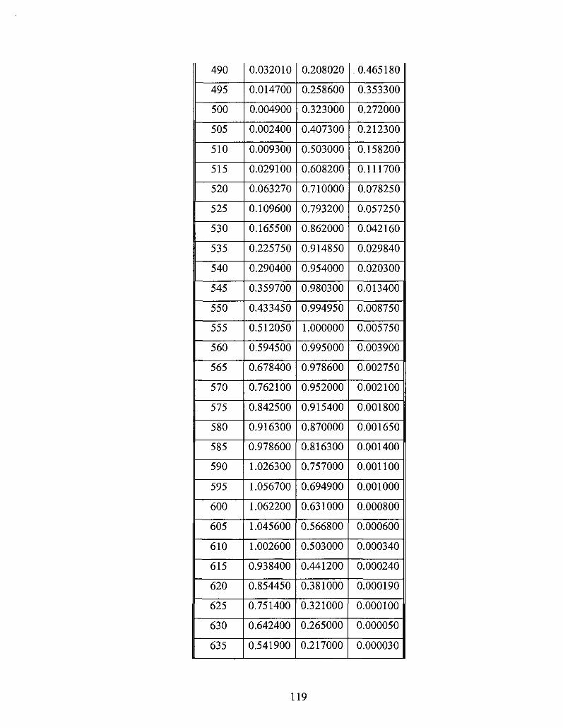
490
495
500
505
510
515
520
525
530
535
540
545
550
555
560
565
570
575
580
585
590
595
600
605
610
615
620
625
630
635
0.032010
0.014700
0.004900
0.002400
0.009300
0.029100
0.063270
0.109600
0.165500
0.225750
0.290400
0.359700
0.433450
0.512050
0.594500
0.678400
0.762100
0.842500
0.916300
0.978600
1.026300
1.056700
1.062200
1.045600
1.002600
0.938400
0.854450
0.751400
0.642400
0.541900
0.208020
0.258600
0.323000
0.407300
0.503000
0.608200
0.710000
0.793200
0.862000
0.914850
0.954000
0.980300
0.994950
1.000000
0.995000
0.978600
0.952000
0.915400
0.870000
0.816300
0.757000
0.694900
0.631000
0.566800
0.503000
0.441200
0.381000
0.321000
0.265000
0.217000
.0.465180
0.353300
0.272000
0.212300
0.158200
0.111700
0.078250
0.057250
0.042160
0.029840
0.020300
0.013400
0.008750
0.005750
0.003900
0.002750
0.002100
0.001800
0.001650
0.001400
0.001100
0.001000
0.000800
0.000600
0.000340
0.000240
0.000190
0.000100
0.000050
0.000030
1 19
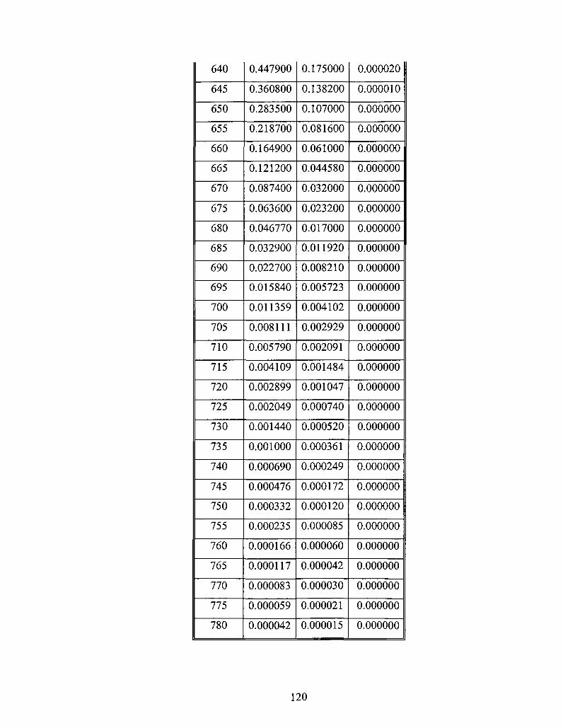
640
645
650
655
660
665
670
675
680
685
690
695
700
705
710
715
720
725
730
735
740
745
750
755
760
765
770
775
780
0.447900
0.360800
0.283500
0.218700
0.164900
0.121200
0.087400
0.063600
0.046770
0.032900
0.022700
0.015840
0.011359
0.008111
0.005790
0.004109
0.002899
0.002049
0.001440
0.001000
0.000690
0.000476
0.000332
0.000235
0.000166
0.000117
0.000083
0.000059
0.000042
0.175000
0.138200
0.107000
0.081600
0.061000
0.044580
0.032000
0.023200
0.017000
0.011920
0.008210
0.005723
0.004102
0.002929
0.002091
0.001484
0.001047
0.000740
0.000520
0.000361
0.000249
0.000172
0.000120
0.000085
0.000060
0.000042
0.000030
0.000021
0.000015
0.000020
0.000010
0.000000
0.000000
0.000000
0.000000
0.000000
0.000000
0.000000
0.000000
0.000000
0.000000
0.000000
0.000000
0.000000
0.000000
0.000000
0.000000
0.000000
0.000000
0.000000
0.000000
0.000000
0.000000
0.000000
0.000000
0.000000
0.000000
0.000000
120