NASDAQ OMX CASH FLOW MARGIN
Methodology guide for margining Nordic fixed income products.
10/31/2011 NASDAQ OMX Stockholm (NOMX)

NASDAQ OMX CASH FLOW MARGIN 2011
2 NASDAQ OMX
DOCUMENT INFORMATION GENERAL READING GUIDELINES The document is mainly divided in two parts; a theoretical part that describes the
basic principles and a practical part that contains margin calculation examples. The
theoretical part has been kept relatively short and many of the mathematical
explanations have, in order to facilitate the reading, been moved to one of the
appendices.
In the calculation examples, we do not try to exactly replicate the margin
calculations performed by the clearing system. The goal is rather to illustrate the
basic concepts of the calculations. For exact replication of CFM, please use the risk
cubes available through Genium Risk’s API, or via interface files.

NASDAQ OMX CASH FLOW MARGIN 2011
3 NASDAQ OMX
TABLE OF CONTENTS Document information ................................................................................................. 2
General reading guidelines ............................................................................ 2
Background .................................................................................................................. 5
Purpose of document .................................................................................... 5
Introduction to clearing ................................................................................. 6
Trading and reporting ...................................................................... 6
Flows between NOMX and the clearing participants ...................... 6
Benefits of central clearing .............................................................. 7
NASDAQ OMX Cash Flow Margin ............................................................................... 10
Executive summary ...................................................................................... 10
Yield curves .................................................................................................. 10
Definition ....................................................................................... 10
Basics ............................................................................................. 11
Bootstrapping ................................................................................ 12
Principal components analysis ...................................................... 14
Calculation Principles ................................................................................... 17
Margin calculations ...................................................................................... 35
Naked margin ................................................................................ 35
Correlation of different yield curves.............................................. 37
Margin calculation examples ..................................................................................... 42
Example 1 ..................................................................................................... 42
REPO transaction with two open legs ........................................... 42
Example 2 ..................................................................................................... 47
REPO transaction with one open leg ............................................. 47
Example 3 ..................................................................................................... 52
Spread position in a REPO transaction .......................................... 52
Example 5 ..................................................................................................... 60
Interest rate swap.......................................................................... 60
Example 6 ..................................................................................................... 66
Interest rate swap versus FRA ....................................................... 66
Example 7 ..................................................................................................... 75
FRA portfolio versus RIBA portfolio ............................................... 75
Example 8 ..................................................................................................... 82
Future contracts with daily settlement ......................................... 82

NASDAQ OMX CASH FLOW MARGIN 2011
4 NASDAQ OMX
Example 9 ..................................................................................................... 87
Bond forward (non synthetic) ....................................................... 87
Example 10 ................................................................................................... 93
Bond forward (synthetic) ............................................................... 93
Appendices ............................................................................................................... 100
Appendix I .................................................................................................. 100
Bootstrapping yield curves using cubic splines ........................... 100
Appendix II ................................................................................................. 103
Principal components analysis .................................................... 103
Appendix III ................................................................................................ 106
One-dimensional window method .............................................. 106
Appendix IV ................................................................................................ 110
A guide to margin replication using interface files ...................... 110

NASDAQ OMX CASH FLOW MARGIN 2011
5 NASDAQ OMX
BACKGROUND PURPOSE OF DOCUMENT This document describes the NASDAQ OMX CFM methodology applied in order to
margin Nordic fixed income instruments. Originally constructed to cater for OTC
derivates, it will shortly be possible for clients to elect to margin their entire fixed
income portfolio with CFM.
The first part of the document describes the basic margin principles and the second
part presents examples on margin calculations. The margin examples will be
performed on both naked positions and on hedged positions.
In one of the appendices, please find a short note on how the interface files can be
used for exact replication of the margin calculations.

NASDAQ OMX CASH FLOW MARGIN 2011
6 NASDAQ OMX
INTRODUCTION TO CLEARING TR A DING AN D R EPO RTI NG
• Customers and primary dealers negotiate the terms of the trades off
exchange.
• Trades are reported to NOMX via a member firm. All trades are registered
in the GENIUM INET clearing system.
• NOMX guarantees that all trades registered in GENIUM INET will be
honored.
TR A N S A C T I O N F L O W S
Figure: Transaction flows.
FLOW S B ET W EEN NOMX AN D T HE CLEA RIN G P ARTI CI PAN TS There are two main flows between NOMX and the clearing participants.
1. Margin – Collateral; NOMX calculates the margin requirement at the end of each trading day (t). The margin requirement becomes available to the clearing participants approximately at CET 22:00 on day t. The clearing participants have to cover their margin requirement with collateral. The clearing participants must have sufficient collateral in place before CET 11:00 on day t+1.
2. Settlement; NOMX provides the clearing participants with settlement instructions. The settlement instructions are normally provided two bank days prior to the settlement day. The cash settlement takes place at CET 11:45 in the Swedish central bank’s electronic cash clearing system for banks (RIX) and the

NASDAQ OMX CASH FLOW MARGIN 2011
7 NASDAQ OMX
bond delivery takes place between CET 06:00 – 14:00 in the Swedish central securities depository (VPC / Euroclear Sweden AB).
MA R G I N A N D S E T T L E M E N T F L O W S
Figure: Margin and settlement flows.
BENEFI TS O F CENTR A L CLEA RIN G Central clearing provides a number of benefits which in the end are increasing
market efficiency and decreasing capital employed.
Credit risk reduction is one key benefit when counterparty exposure is switched
from the trading counterparty to the clearing house. Another key benefit is the
multilateral netting service that the clearing provides. A position taken against a
trading counterparty can be closed out by a trade with another trading
counterparty. Collateral and margins are pledged on a total portfolio basis rather
than on counterparty basis, leading to more efficient capital allocation. The clearing
house also allow for netting of positive and negative margins between asset classes
which can have significant impact on capital employed.
BE N E F I T S F O R P R I M A R Y D E A L E R S
Market makers and banks benefit from central clearing in a number of areas.
Counterparty risk exposure can be significantly reduced and existing counterparty
credit lines can be used for other businesses. The bank can trade with new
counterparties without having to review that counterpart’s credit risk.

NASDAQ OMX CASH FLOW MARGIN 2011
8 NASDAQ OMX
Use of a central clearing service will also mean one position per contract against the
clearing house instead of multiple counterparty positions.
The bank also benefits from one netted collateral/margining which can have
significant impact on capital employment.
One clearing account also means reduced administration when collateral only needs
to be pledged once per day1 against the clearing house instead of multiple pledges
in the non cleared market.
BE N E F I T S F O R I N S T I T U T I O N A L I N V E S T O R S ( C U S T O M E R S)
Central clearing may provide a simplified access for new market institutional
investors since trading with all clearing members can be performed using the same
clearing account structure. No counterparty credit lines are needed.
Counterparty risk exposure can be significantly reduced and existing counterparty
credit lines can be used for other- or new business.
Using a central clearing service also implies that only one netted
collateral/margining amount is needed to be pledged.
BE N E F I T S F O R A U T H O R I T I E S
Central banks and national debt offices are from time to time active in the financial
markets and therefore benefit from reduced counterparty risk exposures as do any
other market participant.
Central banks and FSA’s etc. also have an interest in central clearing from a financial
market stability point of view.
M A R G I N R E Q U I R E M E N T The margin requirement is a fundamental part of CCP clearing. In case of a clearing
participant’s default, it is that participant’s margin requirement together with the
financial resources of NOMX that ensures that all contracts registered for clearing
will be honored.
• NOMX requires margins from all clearing participants, and the margin
requirement is calculated with the same risk parameters regardless of the
clearing participant’s credit rating.
• The margin requirement shall cover the market risk of the positions in the
clearing participant’s account. NOMX applies a 99.2% confidence level and
assumes a liquidation period of two to five days (depending on the
instrument) when determining the risk parameters.
Fixed income instruments show very high correlation, and it is important that the
margin methodology is able to capture this correlation; otherwise the margin
requirements will be too high resulting in an expensive clearing service.
1 NOMX may perform an intra-day margin call. In this case the affected clearing participant must pledge margins an additional time that day.

NASDAQ OMX CASH FLOW MARGIN 2011
9 NASDAQ OMX
Desirable properties of a margin methodology are that it should mirror realistic
circumstances, and at the same time be capital efficient. When margining fixed
income derivatives it appears natural to utilize the strong intra curve correlation.
NOMX CFM (short for NASDAQ OMX CASH FLOW MARGIN) is a yield curve based
margin methodology that captures this correlation of fixed income instruments
priced against the same curve. NASDAQ OMX has initiated NOMX CFM for REPO
transactions and IRS but will shortly include all cleared fixed income products2.
2 Danish MBFs will initially continue to be margined using OMS II.

NASDAQ OMX CASH FLOW MARGIN 2011
10 NASDAQ OMX
NASDAQ OMX CASH FLOW MARGIN EXECUTIVE SUMMARY NASDAQ OMX Cash Flow Margin is a yield curve based margin model. Instead of
stressing each instrument’s individual price, yield curves are stressed using their first
three principal components. All instruments in an account are then evaluated
against each stressed yield curve and the margin requirement is given as the
combined value of these instruments calculated with the worst of the stressed yield
curves.
• REPO: A REPO transaction will be treated as a sold/bought spot contract
and a corresponding bought/sold forward contract. The spot price will be
calculated from the corresponding yield curve
• IRS: An interest rate swap will be treated as a series of future cash flows.
All swap cash flows will be evaluated against the same curve giving optimal
netting benefits between an account’s different interest rate swaps.
• FRA: A forward rate agreement will be treated as one fixed and one
floating cash flow. The floating flow will be forecasted using the swap curve
and the contract will be priced using the same curve as for the interest rate
swaps
• Bond-forward: A bond forward will be priced against the bond’s
corresponding yield curve. Since the bond forwards are not used for curve
construction there will be a small difference between the traded yield of
the bond forwards, and the estimated forward yield from the cash flow
analysis
• Options on FRAs and Bond-forwards: The underlying rate/yield will be
stressed in the ways described above, and then an option pricing formula
will be applied to determine the stressed NPV of the option.
• RIBA-future: A Riksbanks future will be treated as one fixed and one
floating cash flow. The floating flow will be forecasted using the RIBA curve.
No discounting of cash flows will take place.
• CIBOR-future: A CIBOR future will be treated as one fixed and one floating
cash flow. The floating flow will be forecasted using the CIBOR curve. No
discounting of cash flows will take place.
YIELD CURVES A key part to NOMX CFM is the ability to calculate the present value of future cash
flows. Yield curves are needed in order to do this. This section describes how NOMX
obtains the yield curves from instrument prices as well as the method applied in
order to stress the curves.
DEFINI TION The yield curve (or more formally the term structure of interest rates) is defined as
the relation between the interest rate that lenders require for lending out capital at
different maturities. This relationship will of course differ depending on the credit
quality of the borrower, and it therefore exist several yield curves in each currency.

NASDAQ OMX CASH FLOW MARGIN 2011
11 NASDAQ OMX
BA SI CS The yield curve is divided into a short end (all maturities up to two years) and a long
end. A common view is that the short end of the yield curve is under the control of
the central bank, whereas the long end is much more under the influence of the
future inflation anticipated by long term fixed income investors.
Yield curves can be used to extract various types of information:
• Expectation on future short-term rates: Although a yield curve may not
necessarily reveal all information on investors’ view of future short-term
rates, it is possible to draw conclusions on this view based on the shape of
the yield curves.
• Probability of default: The treasury curve, i.e. the yield curve derived from
government securities, is in developed markets often assumed to be free
from credit risk. The spread between a treasury curve and the yield curve
for a financial institution can therefore be used to deduct the market’s
view of the probability of default for that financial institution.
Underlying price carrier: Since the yield curve is derived from instrument prices it
can also be used to price fixed income instruments. This is the most important
feature of the yield curve and it is in this sense that NOMX will use the yield curves.

NASDAQ OMX CASH FLOW MARGIN 2011
12 NASDAQ OMX
BOOTS TR APPI NG Bootstrapping is a methodology that is used to extract the yield curves from the
market prices of fixed income instruments.
B A S I C D E F I N I T I O N S
The basic definitions regarding bootstrapping are presented below.
IN S T R U M E N T S
A fixed income instrument is defined as a set of rules concerning future cash flows.
Prices are quoted on the fixed income instruments and their prices reveal
information on the expected return for investing in these instruments. Typical fixed
income instruments include bills, bonds, interest rate swaps, and forward rate
agreements among others.
C O M P O U N D I N G F R E Q U E N CY A N D DA Y C O U N T C O N V E N T I O N
NOMX expresses all yield curves as yearly compounded interest rates with day
count convention ACT/365.
D I S C O U N T F U N C T I O N
The discount function,��������, is defined as the price today of a zero-coupon
bond that pays $1 at the value date, T. The discount function is a decreasing
function of time to maturity,��� ��� ����� , and by definition it starts at 1.
Figure: Discount function for different time to maturities.
SP O T R A T E
The spot rate, �������, is defined as the yearly compounded interest rate for a
zero-coupon bond that is traded today, and that matures at the value date, T.
Equation (1) relates the spot rate to the discount function.
������� � ������������ � � 1
0
0.2
0.4
0.6
0.8
1
1.2
00.
5 11.
5 22.
5 33.
5 44.
5 55.
5 66.
5 77.
5 88.
5 99.
5 10
NASDAQ OMX CASH FLOW MARGIN 2011
13 NASDAQ OMX
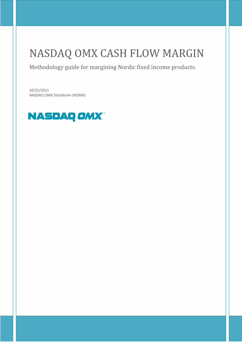
Figure: Spot rate for different time to maturities.
F O R W A R D- F O R W A R D R A TE
The forward-forward rate � ������ ������ is defined as the yearly compounded
implied forward rate on an investment that:
• Is traded today.
• Starts at the settlement date, t.
• Ends at the value date, T.
Equation (2) relates the forward-forward rate to the spot rate.
����������� ��� ������������ ���������� ����!�� � � 2
BO O T S T R A P P I N G P R O C E D U R E
The typical procedure is to bootstrap the discount function. Equation (1) – (2) can
then be used to obtain the spot- and the forward-forward rates from the discount
function.
NOMX will use the following fixed income instruments as “calibration instruments”
in the bootstrapping procedure.
• Bills and bonds will be used to bootstrap the treasury and mortgage curves.
• Deposits, forward rate agreements or interest rate futures, and interest
rate swaps will be used to bootstrap the swap curves.
• RIBA futures will be used to bootstrap an implicit RIBA (repo rate) curve.
Please see Appendix I for a detailed description of the bootstrapping methodology
applied by NOMX.
0.00%
0.50%
1.00%
1.50%
2.00%
2.50%
3.00%
3.50%
4.00%
00.
5 11.
5 22.
5 33.
5 44.
5 55.
5 66.
5 77.
5 88.
5 99.
5 10

NASDAQ OMX CASH FLOW MARGIN 2011
14 NASDAQ OMX
PRIN CIP A L CO MPO N EN TS A NA LYSI S The present value of a future cash flow, exposed to a given yield curve; will change
if the shape of the yield curve changes. A yield curve may change in numerous ways,
but there is empirical evidence that the curve’s first three principal components
express the vast majority of the changes.
This section defines the first three principal components from an economical point
of view and further gives a brief overview of how NOMX will use the principal
components to stress the yield curves in the margin calculations.
Appendix II gives a more in-depth description of the principal component analysis.
EC O N O M I C A L D E F I N I T I O N O F T H E P R I N C I P A L C O M P O N E N T S
Principal components (PC) are defined as independent (uncorrelated) moves of the
yield curve.
PC1: PA R A L L E L S H I F T
For a yield curve the first PC is a parallel shift of the entire curve. This PC usually
explains 75%-85% of the curve’s historical movement. This is also quite
understandable, that economic factors that changes cause the interest rate market
as a whole to increase or decrease.
PC2: C H A N G E I N S L O P E
The second PC is a change to the slope of the curve. The long end goes up while the
short end goes down or vice versa. This PC usually explains 10%-15% of the curve’s
historical movement.
PC3: C H A N G E I N C U R V A T U R E
The third PC is a change to the curvature of the curve. The short and the long end
increase while the mid section decrease or vice versa. This PC usually explains 3%-
5% of the curve’s historical movement.
Figure: A yield curve’s first three principal components.
-0.6
-0.4
-0.2
0
0.2
0.4
0.6
0.8
1
1.2
00.
5 11.
5 22.
5 33.
5 44.
5 55.
5 66.
5 77.
5 88.
5 99.
5 10
PC1 PC2 PC3
NASDAQ OMX CASH FLOW MARGIN 2011
15 NASDAQ OMX
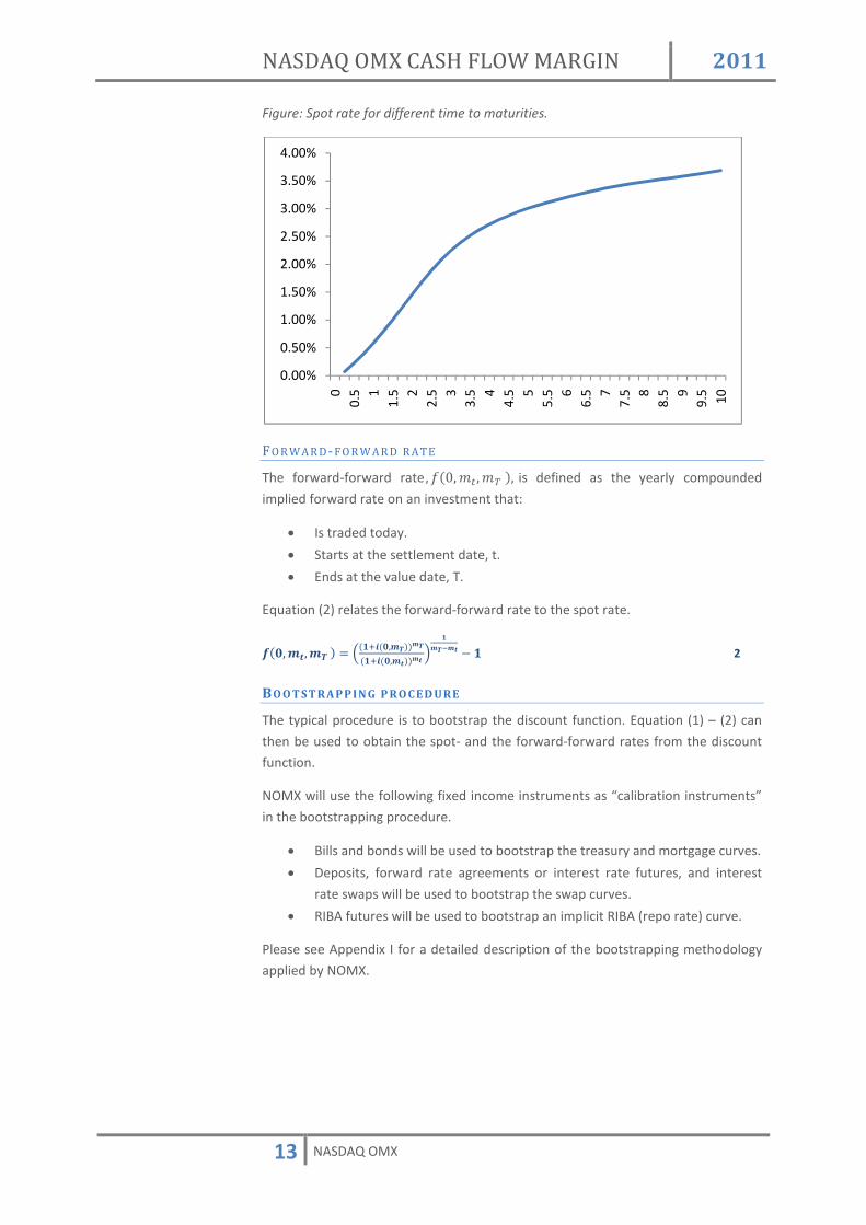
S T R E S S I N G A C U R V E W I T H I T S P R I N C I P A L C O M P O N E N T S
A yield curve’s principal components are by definition uncorrelated. The first three
principal components explain the majority of the variance which implies that a
linear combination of the principal components can be used to simulate curve
changes with high accuracy3.
NOMX will, on a quarterly basis, evaluate and, if needed, update each yield curve’s
first three principal components together with a risk parameter that decides how
much of this principal component that will be used to simulate the stressed curves.
A risk parameter of 22 basis points in PC1 will for example imply that the curve will
be stressed with a parallel shift of 22 basis points upwards and downwards.
Figure: Stressing a curve with its first PC i.e. by different levels of parallel shifts.
Figure: Stressing a curve with its second PC i.e. by different levels of slope changes.
3 This statement has been validated with back testing calculations performed by NOMX.
-25
-20
-15
-10
-5
0
5
10
15
20
25
0
0.5 1
1.5 2
2.5 3
3.5 4
4.5 5
5.5 6
6.5 7
7.5 8
8.5 9
9.5 10
-10
-8
-6
-4
-2
0
2
4
6
8
10
0
0.5 1
1.5 2
2.5 3
3.5 4
4.5 5
5.5 6
6.5 7
7.5 8
8.5 9
9.5 10

NASDAQ OMX CASH FLOW MARGIN 2011
16 NASDAQ OMX
Figure: Stressing a curve with its third PC i.e. by different levels of curvature changes.
NOMX will on each trading day, t, bootstrap official spot curves (Curvet). These
curves will be the basis to all stressed curves. Equation (3) will be used to simulate
the stressed curves from the official curves. NOMX defines the yield curves and their
principal components as vectors. Equation (3) is therefore a vector equation were
each element is handled separately. The margin calculation examples in the end of
this document describe this process in more detail.
"#$%&'''''''''(�$&))&� "#$%&'''''''''� * + , -"�'''''' * . , -"/'''''' * 0 , -"1'''''' 3
a, b and c will range between ± each principal component’s risk parameter.
AP P L Y I N G A BU Y & S E L L S P R E A D
NOMX has the ability to apply a spread to the curves used for margining. Depending
on the instrument being priced, this spread will be applied in a different step in the
process.
For derivatives with bonds as underlying instruments the spread will be applied
when discounting the fixed cash flows stemming from the bond. This is the case for
repos and bond forwards.
For derivatives with floating cash flows the spread will be applied when forecasting
the sizes of these cash flows. This is the case for swaps, forward rate agreements,
RIBA futures, STIBOR-futures and CIBOR-futures.
-6
-4
-2
0
2
4
6
0
0.5 1
1.5 2
2.5 3
3.5 4
4.5 5
5.5 6
6.5 7
7.5 8
8.5 9
9.5 10

NASDAQ OMX CASH FLOW MARGIN 2011
17 NASDAQ OMX
CALCULATION PRINCIPLES At the core of NOMX CFM are the cash flows of the instruments. For all instruments,
an important step in the calculation is to identify these flows, and categorize them
as floating or fixed. They are then inserted in a cash flow table.
Subsequently the cash flows are used in various ways for different instruments.
Below we describe these procedures that in the end lead to a calculated margin.
DE F I N I T I O N O F C A S H F L O W T A B L E S
A cash flow table is an object with the following properties.
• Curve exposure; a reference to the yield curve that the cash flows in this
table are exposed to. This is the curve that will be used when discounting
these cash flows and when determining the size of the floating cash flows.
• Currency; each column in the cash flow table represent the currency of the
cash flows.
• Value date; each row in the cash flow table represent the value date of a
cash flow.
Figure: Example of a treasury cash flow table.
Value date SEK
2010-03-15 23�2������ … … 2011-03-15 4��23�2������
BR E A K U P A L G O R I T H M S
REPO
DE F I N I T I O N S
Standard = Defines if this is a “classic REPO” or a “buy and sell back”. T = Trade date. ts = Start date. te = End date. tm = Maturity date of the underlying bond. tc = Date of the underlying bond’s last coupon payment. di,j = Number of days between dates ti and tj (30E). Q = Quantity. N = Nominal amount of the underlying bond. C = Coupon of the underlying bond. Side = 5 4��67�8�9:;<=�����������������4��67�8�7>?>7@>��9:;<=A CPt = Underlying bond’s clean price at time t. rrepo = Contracted repo rate. Ci = Underlying bond’s payment at value date ti. Xs = Start consideration. Xe = End consideration. Rowi = Cash flow table value for value date ti.

NASDAQ OMX CASH FLOW MARGIN 2011
18 NASDAQ OMX
F O R M U L A S
S T A R T C O N S I D E R A T I O N
Equation (4) is used to calculate the start consideration for both a classic REPO and
for a buy and sell back.
B) �"- * " , ��0��)1C� � , D��� , E 4
Note that if ex-coupon date has passed, the accrued interest will be negative
E N D C O N S I D E R A T I O N
C L A S S I C R E P O
Equation (5) is used to calculate the end consideration for a classic REPO.
B& B) , �� * $$&FG , �)�&1C�� 5
B U Y A N D S E L L B A C K
Equation (6) is used to calculate the end consideration for a buy and sell back.
B& B) , �� * $$&FG , �)�&1C�� � "� , �� * $$&FG , ���&1C�� 6
It is only the underlying bond’s payments, Ci, that are on value dates, ti, in the
interval [ts+5, te+5] that should be included in Equation (6).
C L A S S I C R E P O
Equation (7) - (8) will be used to insert the start and end considerations into the
start and end consideration cash flow table.
HGI) (��& , B) 7
HGI& �(��& , B& 8
Equation (9) will be used to insert the underlying bond’s payments, Ci, that are on
value dates ti in the interval [ts+5, te+5] into the start and end consideration cash
flow table.
HGI� (��& , "� 9
B U Y A N D S E L L B A C K
Equation (7) – (8) will be used to insert the start and end considerations into the
start and end consideration cash flow table.

NASDAQ OMX CASH FLOW MARGIN 2011
19 NASDAQ OMX
B O N D C A S H F L O W T A B L E
The underlying bond will be exchanged two times in a REPO transaction, on the start
date and on the end date.
S T A R T D A T E
C L A S S I C R E P O
Equation (10) will be used to insert the cash flows originating from the underlying
bond that is exchanged on the start date into the bond cash flow table.
HGI� �(��& , E , "� ��G$�+JJ�"���K+��J+L��M)��&N�& * O� ��P 10
B U Y A N D S E L L B A C K
Equation (11) will be used to insert the cash flows originating from the underlying
bond that is exchanged on the start date into the bond cash flow table.
HGI� �(��& , E , "� ��G$�+JJ�"���K+��J+L��M)��&N�) * O� ��P 11
E N D D A T E
Equation (12) will be used to insert the cash flows originating from the underlying
bond that is exchanged on the end date into the cash flow table.
HGI� (��& , E , "� ��G$�+JJ�"���K+��J+L��M)��&N�& * O� ��P 12
E X A M P L E
Considerer a one week REPO in RGKB1045.
Standard = Buy and sell back. t = 2009-11-02. ts = 2009-11-04. te = 2009-11-11. tm = 2011-03-15. tc = 2009-03-15. Q = 1 000. N = SEK 1 000 000. C = 5,25. Side = 1. CP = 105,89. rrepo = 0,25%. Ci = Payment 52 500 1 052 500
Date 2010-03-15 2011-03-15
S T A R T C O N S I D E R A T I O N
Equation (4) is used to calculate the start consideration. It is 229 days between
2009-03-15 and 2009-11-04 in a 30E convention.
QR �4�2�ST * 2�32 , UUV��W� , X�WWW�WWWXWW , 4��� Y:Z�4��T3�3T2�S[[
E N D C O N S I D E R A T I O N
Equation (6) is used to calculate the end consideration.
Q\ 4��T3�3T2�S[[ , �4 * ��32] , ^��W� Y:Z�4��T3�[_S�T[4

NASDAQ OMX CASH FLOW MARGIN 2011
20 NASDAQ OMX
This would result in the following cash flow table.
S T A R T A N D E N D C O N S I D E R A T I O N C A S H F L O W T A B L E ( E X P O S E D T O T H E T R E A S U R Y C U R V E )
Equation (8) – (9) is used to insert the start and end considerations into the start
and end consideration cash flow table.
Value date SEK 2009-11-04 1 · 1 092 295 833 = 1 092 295 833 2009-11-11 -1 · 1 092 348 931 = -1 092 348 931
T R E A S U R Y C A S H F L O W T A B L E
Before the start date of the REPO, the underlying bond will not have been
exchanged, and since the underlying bond does not pay any coupons in the interval
[ts+5, te+5]the cash flows from Equation (11) and Equation (12) will cancel out each
other. The bond cash flow table will therefore be empty until after the start date of
the REPO.

NASDAQ OMX CASH FLOW MARGIN 2011
21 NASDAQ OMX
IN T E R E S T R A TE S W A P S
The cash flows of a fixed for floating interest rate swap are exposed to the swap
curve. Equations (13) - (16) are used to break up a fixed for floating interest rate
swap.
DE F I N I T I O N S
t = Trade date. ts = Start date. te = End date. Q = Quantity. N = Principal amount. Side = 54����`a>�@b8c��@�d6efa`=�4����`a>�@b8c��@�@6g�= A ri,i+1 = Forward-forward swap rate valid from ti to ti+1. di,i+1 = Number of days in the floating interest rate period between value
dates ti and ti+1 (ACT). rfl = First floating interest rate (this is known at the time when the swap
is entered). rf = Fixed contracted rate of the interest rate swap. df,i,i+1 = Number of days in the fixed interest rate period between value
dates ti and ti+1 (30E). Rowi = Cash flow table value for value date ti.
E Q U A T I O N S
F L O A T I N G C A S H F L O W S
HGI� � (��& , E , D , $��� � , ����h�1C� 13
The forward-forward rate� 7i�i X� is a function of the swap spot rate. This implies that 7i�i X will be updated each time the swap spot rate is updated. A floating cash flow
will therefore be updated for each stressed curve that is used in the margin
calculations.
It should be noted that 7i�i Xdoes not use the same compounding frequency
compared to the forward-forward rate� �����i � �i X�, defined in Equation (2).
Equation (14) relates the two forward rates.
$��� � 1C�����h� , ��� * ��������� �����h��� � �� 14
F I X E D C A S H F L O W S
F I R S T F L O A T I N G I N T E R E S T R A T E
The first floating interest rate is known at the time when the swap is entered. The
first floating cash flow is therefore in reality a fixed cash flow.
HGI� (��& , E , D , $�J , ����1C� 15
F I X E D C O N T R A C T E D I N T E R E S T R A T E HGI� � �(��& , E , D , $� , ������h�1C� 16

NASDAQ OMX CASH FLOW MARGIN 2011
22 NASDAQ OMX
E X A M P L E
Consider a sold 3Y plain vanilla SEK fixed for floating interest rate swap.
t = 2009-11-02 ts = 2009-11-04. te = 2012-11-04. Q = 5 N = SEK 1 000 000 Side = -1 rfl = 0,3% rf = 1,7%
This would result in the following cash flow table. It should be noted that since the
first floating cash flow is in fact a fixed cash flow it is moved to the fixed side. It
should further be noted that the floating cash flows will be updated when the swap
spot curve changes.
S W A P C A S H F L O W T A B L E
Value date SEK (floating) SEK (fixed)
2010-02-04 �4 , 2� , 4��������� , ��[] , T3[j�
2010-05-04 �4 , 2� , 4��������� , 7X�U , ST[j�
2010-08-04 �4 , 2� , 4��������� , 7U�� , T3[j�
2010-11-04 �4 , 2� , 4��������� , 7��k , T3[j� 4 , 2� , 4��������� , 4�l] , [j�[j�
2011-02-04 �4 , 2� , 4��������� , 7k�� , T3[j�
2011-05-04 �4 , 2� , 4��������� , 7��� , ST[j�
2011-08-04 �4 , 2� , 4��������� , 7��^ , T3[j�
2011-11-04 �4 , 2� , 4��������� , 7̂ �m , T3[j� 4 , 2� , 4��������� , 4�l] , [j�[j�
2012-02-06 �4 , 2� , 4��������� , 7m�V , T_[j�
2012-05-04 �4 , 2� , 4��������� , 7V�XW , SS[j�
2012-08-06 �4 , 2� , 4��������� , 7XW�XX , T3[j�
2012-11-05 �4 , 2� , 4��������� , 7XX�XU , T3[j� 4 , 2� , 4��������� , 4�l] , [j�[j�

NASDAQ OMX CASH FLOW MARGIN 2011
23 NASDAQ OMX
F O R W A R D R A T E A GR E E M E N T S
A forward rate agreement (FRA) is a forward contract on a fictive forward loan i.e. a
view on the future 3MSTIBOR rate. There is no delivery of the underlying loan
amount. Only a cash amount corresponding to the interest rate difference between
agreed interest rate and the fixing rate will be paid. The buyer of the contract is a
fictitious borrower who assumes the obligation to pay the difference between the
agreed interest rate and the fixing rate to the seller on condition that the agreed
interest rate is higher. If the agreed interest rate is lower than the fixing rate, the
buyer is paid the interest rate amount by the seller. The amount is valued three
months after the expiration of the FRA contract. However, the actual payment is
settled on the settlement day of the FRA contract three months earlier. This means
that the valued amount needs to be discounted to the settlement day of the FRA
contract.
Equations (17) – (18) are used to insert a FRA into the FRA cash flow table.
DE F I N I T I O N S
t = Trade date. tm = Maturity date of the FRA. Q = Quantity. N = Principal amount of the fictive loan. Side = 54����`a>�n9o��@�d6efa`=�4����`a>�n9o��@�@6g�= A ri,i+1 = Forward-forward swap rate between ti and ti+1. di,i+1 = Number of days in the floating interest rate period between
value dates ti and ti+1 (30E). rc = Contracted rate of the FRA. PnLFRA(ri,i+1,rc) = Profit and loss of a FRA contract given a forward-forward rate,
ri,i+1, and a contracted rate, rc. Rowm = Cash flow table value for value date tm.
F O R M U L A S
It should be noted that 7i�i X is defined with a different compounding frequency
compared to������i � �i X�. Equation (14) relates the two forward-forward rates.
-MpqHr�$��� �� $0� (��& , E , D , �$��� � � $0� , ����h�1C� 17
HGI� -MpqHr�$���h��$0��� $���h�s����h�1C� � 18

NASDAQ OMX CASH FLOW MARGIN 2011
24 NASDAQ OMX
E X A M P L E
Consider 100 bought FRA09X contract.
t = 2009-11-02 tm = 2009-12-16 Q = 100 N = SEK 1 000 000 Side = 1 rc = 0,4%
This would result in the following FRA cash flow table. The FRA cash flow is a
floating cash flow and hence it is updated as the swap spot curve changes.
F R A C A S H F L O W T A B L E ( E X P O S E D T O T H E S W A P C U R V E )
Value date SEK (floating) 2009-12-17 ;tuvwx�7UWWVXUX��UWXWW�X^� 7y��4 * 7UWWVXUX��UWXWW�X^ s �i�i X[j� �

NASDAQ OMX CASH FLOW MARGIN 2011
25 NASDAQ OMX
OP T I O N S O N F O R W A R D R A T E A G R E E ME N T S
The pricing of the FRA options builds on the same methodology used to price the
FRAs. The method for estimating the forward rate is exactly the same. Given an
estimated rate (rest), the calculation of the NPV for a specific option is given by the
following calculations.
DE F I N I T I O N S
Q = Quantity of underlying contracts N = Nominal contract size T = Time to expiry dFRA = Length of underlying FRA, measured in days
rS = Strike expressed as forward yield rest = Forward yield estimated from the curve σr = Yield volatility p = Value of option, expressed in yield BPV = Basis point value of underlying FRA
F O R M U L A S
The strike rate, the estimated rate given by the curve, the rate volatility and the
time to expiry are entered into a binomial option pricing formula. The result from
the binomial pricing formula is the price of the option expressed in yield. In order to
convert this premium to a cash measure, the BPV of the underlying FRA is used. For
the FRA options a constant BPV per contract, as defined below, is used. That is, no
convexity effects are taken into account.
z {|}~�|������ ����� ��� �� 19
{�� ������W 4����� ������������������������������������������������������������������������������������20
��� {�� s z s 4�� s � s ������������������������������������������������������������������21

NASDAQ OMX CASH FLOW MARGIN 2011
26 NASDAQ OMX
R I B A F U T U R E
A riba future is a daily cash-settled contract on the Riksbank’s repo rate. The
contract base is a fictious loan extending between two consecutive IMM-dates, and
the price is quoted as a compound interest. The final fix of each future is
determined by the repo rate between the IMM-date of the contract’s end month
and the preceding IMM-date. Therefore, during the last three months of a
contract’s life, the price risk is gradually decreasing as the final fix is increasingly
made known. CFM will pick up this feature through taking into consideration the
historic repo-rate when constructing and stressing the curves. In CFM, the RIBA
futures will be margined using a designated riba curve, built from the prices on the
riba contracts.
Equations (22) – (23) are used to insert a RIBA into the RIBA cash flow table.
DE F I N I T I O N S
tm = Maturity date of the RIBA i.e. the IMM-date of the contract’s end month.
tm-1 = Preceding IMM-date. tfix = The highest date to which the Riksbank’s repo-rate is known.
Note that this can be a future date. Q = Quantity. N = Principal amount of the fictive loan. Side = 54����`a>�9��o��@�d6efa`=�4����`a>�9��o��@�@6g�= A ri,i+1 = Forward-forward repo rate between ti and ti+1. Ri,i+1 = Historic repo rate between ti and ti+1 ,expressed as a
compounded rate. rfirst = Estimated rate for the first RIBA contract. di,i+1 = Number of days in the floating interest rate period between
value dates ti and ti+1 (ACTUAL). rc = Contracted rate of the RIBA i.e. the last fixing of the RIBA. PnLFRA(ri,i+1,rc) = Profit and loss of a RIBA contract given a forward-forward rate,
ri,i+1, and a contracted rate, rc.
F O R M U L A S
For all contracts except the front contract, the P/L is calculated in a straight forward
way.
-MpH��r�$����� $0� (��& , E , D , �$���� � $0� , ��!���1C� 22
For the front contract, we will take into consideration the historic repo rate from
the preceding IMM-date up to the highest date to which the Riksbank’s repo rate
has been determined. We use this information to calculate an estimated rate for the
first RIBA contract. Then the P/L can be calculated as above.
NASDAQ OMX CASH FLOW MARGIN 2011
27 NASDAQ OMX
������ ��� * H������ , ��!�����1C� � , �� * $����� , ������1C� � � ��� , 1C���!��� 23
-MpH��r�$��$)�� $0� (��& , E , D , �$��$)� � $0� , ��!���1C� 24
As the RIBA is a futures contract, the P/L does not need to be added into a cash flow
table in order to calculate the NPV.
E X A M P L E 1
For value date 2011-09-05, consider 100 bought RIBAZ1 contract
R I B A Z1.
tm = 2011-12-21 tm-1 = 2011-09-21 Q = 100 N = SEK 1 000 000 Side = 1 rc = 2,04%
Since in this example, the start date of the underlying IMM-period is in the future,
we only have to take the estimated forward repo rate into consideration. There are
91 days in the underlying period. Given a RIBA curve, the P/L of this RIBA future is
given by the following formula.
;tuw ¡x�7UWXXWVUX�UWXXXUUX� 3��_]�
4 , 4�� , 4������� , �7UWXXWVUX�UWXXXUUX � 3=�_]� , T4[j�
E X A M P L E 2
For value date 2011-09-05, consider 100 bought RIBAU1 contract.
R I B A U1
tm = 2011-09-21 tm-1 = 2011-06-15 tfix = 2011-09-07 Q = 100 N = SEK 1 000 000 Side = 1 rc = 1,96%
Since in this example, the start date of the underlying IMM-period is in the past, we
have to take the historic repo rate into account. For the first three weeks (from
2011-06-15 to 2011-07-06) the weekly repo rate was 1,75%, and for the remainder
of the period until 2011-09-07 it was 2%, resulting in a compound average rate of
1,94%. There are 98 days in the underlying period, and for the first 84 of these the
repo rate is known. Given a RIBA curve, the P/L of this RIBA future is given by the
following calculation in two steps.

NASDAQ OMX CASH FLOW MARGIN 2011
28 NASDAQ OMX
������� ��� * �� ¢£] , ¤£1C�� , �� * $/����¢�¥�/����¢/� , �£1C�� � ��� , 1C�¢¤
���������������������������������-MpH��r�$��$)�� �� ¢C]� � , ��� , ��������� , �$��$)� � �� ¢C]� , ¢¤1C�

NASDAQ OMX CASH FLOW MARGIN 2011
29 NASDAQ OMX
CIB OR/ STIB OR F U T U R E
NOMX offers clearing of interest rate futures with the 3M Deposits of CIBOR and
STIBOR as underlyings. These futures are quoted as [100-yield], which means that
their P/L dynamics are similar to that of cash bonds. In contrast to the other cleared
derivatives with single period forward rates as underlyings (RIBA futures and FRAs),
an increase in the estimated underlying rate results in a negative P/L. For example, a
long position in a STIBOR future can be hedged by a long position in a FRA for the
same period. The CIBOR/STIBOR Futures always have an underlying period of 90
days, independently of the actual number of days between the IMM-days.
DE F I N I T I O N S
t = Trade date. tm = Maturity date. Q = Quantity. N = Principal amount of the fictive loan. Side = 54����`a>��e`e7>��@�d6efa`=�4����`a>��e`e7>��@�@6g�= A ri,i+1 = Forward-forward swap rate between ti and ti+1. Pc = Daily fix rc = Contracted rate of the FRACIBOR/STIBOR Future. Rowm = Cash flow table value for value date tm. The daily fix is quoted in price (100-median value in yield) i.e. (100 - r). The cash
flows are decided by the formulas:
$0 ��� � -0��������������������������������������������������������������������������������������������������������������������25
-Mp¦� ¡§w�$��� �� $0� (��& , E , D , �$0 ��$��� �� , VW1C� 26
As we are here dealing with futures contracts, the P/L doesn’t need to be added to
any cash flow table for discounting purposes.
E X A M P L E 1
For value date 2011-09-02, consider 100 sold 3MSTIBZ1 contracts.
3M S T I B Z1
t = 2011-09-02. tm = 2011-12-21. Q = 100. N = 1 000 000. Side = -1. d1,2 = 90. Pc = 97,559 rc = 2,441%
;tu�¨¦� ¡©X�7UWXXXUUX�UWXUW�UX� 3�__4]�
�4 , 4�� , 4������� , �3�__4] ��7UWXXXUUX�UWXUW�UX� , T�[j�

NASDAQ OMX CASH FLOW MARGIN 2011
30 NASDAQ OMX
B O N D F O R W A R D S
NASDAQ OMX has two types of bond forwards; synthetic and non synthetic. The
non synthetic bond contract has remaining maturity and coupon rate equal to the
deliverable bond in each series. The synthetic bond forward contracts have a
maturity of two, five or ten years and a fixed annual coupon rate.
It should be noted that the NPV is calculated from a yield curve built up using prices
on cash bonds. The bond forward contracts are not used as calibration instruments
and thus the unstressed NPV will slightly deviate from the market value. However,
the market value presented in margin reports for the bond forwards will be
calculated from equation (19) based on the difference between the traded price (r)
and today’s fixed price (rt).
The synthetic bond forward contract is traded on the forward yield of the
deliverable bond, but the P/L is calculated using the characteristics of the synthetic
bond. Using CFM to calculate margin for these contracts therefore requires some
additional steps compared to the usual cash flow forecasting and discounting used
for most other interest rate derivatives. In short, the cash flows of the synthetic
bond forward will be forward valued, not by using the yield curve, but by using the
forward yield to maturity of the deliverable bond as implied by the yield curve.
M O N T H L Y C A S H S E T T L E M E N T
The fixed income forwards are hybrid futures/forward contracts. The hybrid style arises from the fact that the contract is not settled daily; instead a monthly cash settlement is carried out. This means that margin calculations for fixed income forwards must consider the trade yield or the previous month fixing yield depending on if the trade was carried out during the month or previous to the last monthly cash settlement. At the end of each month the accrued profit and losses on all fixed income forwards contracts are settled at a closing yield for that month, the monthly fixing yield. This effectively revalues open positions to the monthly fixing yield, which is the yield used when calculating subsequent margin requirements.
DE F I N I T I O N S
t = Day t n = Outstanding coupons N = Nominal value C = Coupon rate Q = Number of contracts r = Yield (contracted yield or the last monthly cash settlement
yield, whichever applicable) rt = Fixing yield at day t d = Number of days between the contract’s settlement date
(IMM) and next coupon payment (30E) de = The forward contract’s expiration date dsett = The forward contract’s settlement day
dc = Next coupon date Ci = Underlying bond’s payment at value date ti

NASDAQ OMX CASH FLOW MARGIN 2011
31 NASDAQ OMX
F O R M U L A S
Equation (19) is used to convert a price quoted in yield to a price in money
ª«¬®��� ¯ , �°�,��� ���� ��±�� ��� ®1C�h!��² 27
The first cash flow is decided by the trade price (contracted yield) and will be
executed on the IMM date, usually t+4 for Swedish bond forwards. All upcoming
coupons after the settlement date of the delivery, plus the nominal at end should
also be considered as cash flows4.
Equation (20) is used for synthetic forward contracts to calculate the forward price
quoted in yield of the deliverable bond. The forward yield to maturity, y, is the
solution to the following equation.
°³�´��µ¬¶��� ����·�·����� * °³�´��µ¬¶�h��� ����·�·�h�����h� *¸* °³�´��µ¬¶�h�� ����·�·�h����h °³�´��µ¬¶��� ¹��� * °³�´��µ¬¶�h��� ¹���h� *¸*°³�´��µ¬¶�h�� ¹���h 28
where the day count convention is 30E.
E X A M P L E N O N S Y N T H E T I C B O N D F O R W A R D
Consider the below portfolio of 100 sold NBHYP2 (2-year Nordbanken Hypotek
Bond) contracts
t = 2011-02-15 n = 3 N = SEK 1 000 000 C = 4,25. Q = 100 r = 3,50% rt = 3,55% d 93 de = 2011-03-10 dsett = 2011-03-16 dc = 2011-06-19
Ci =
Payment 42 500 42 500 1 042 500
Date 2011-06-19 2012-06-19 2013-06-19
Equation (19) is used to calculate the trade price. It is 93 days between 2011-03-16
and 2011-06-19 in a 30E convention.
4 If the deliverable bond has a coupon payment less than 5 days from the final settlement of the forward contract, then the original owner of the deliverable bond will receive the coupon payment. In this scenario one coupon payment shall be removed from the mark to market amount.

NASDAQ OMX CASH FLOW MARGIN 2011
32 NASDAQ OMX
;º�» �[�2�]� 4������� , �_�32][�2�] , ��4 * [�2�]�� � 4� * 4�
��4 * [�2�]�� V���W �X�� 4��_l�[TS
This would result in the following cash flow table.
Value date SEK
2011-03-16 -100 · 1 046 215 = -104 739 800
2011-06-19 100 · 42 500 = 4 250 000
2012-06-19 100 · 42 500 = 4 250 000
2013-06-19 100 · (42 500 + 1000 000) = 104 250 000
E X A M P L E S Y N T H E T I C B O N D F O R W A R D
Consider the below portfolio of 100 sold R2RR (government bond) contracts. The
forward contract is traded on the forward yield of the deliverable bond and thus the
bond forward will be valued by using the forward yield to maturity of the
deliverable bond as implied by the yield curve. The deliverable bond for R2RR is
RGKB1041 with maturity 2014-05-05 and a coupon rate of 6,75%.
t = 2011-03-02 n = 3 N = SEK 1 000 000 C = 6,75. Q = -100 r = 2,99% rt = 2,99% d = 320 de = 2011-06-09 dsett = 2011-06-15 dc = 2012-05-05 Ci =
Payment 67 500 67 500 1 067 500
Date 2012-05-05 2013-05-05 2014-05-05
Equation (19) is used to calculate the trade price. It is 320 days between 2011-06-15
and 2012-05-05 in a 30E convention.
;º�» �3�TT]� 4������� , �j�l2]3�TT] , ��4 * 3�TT]�� � 4� * 4�
��4 * 3�TT]���UW��W �X�� 4�44����_
NASDAQ OMX CASH FLOW MARGIN 2011
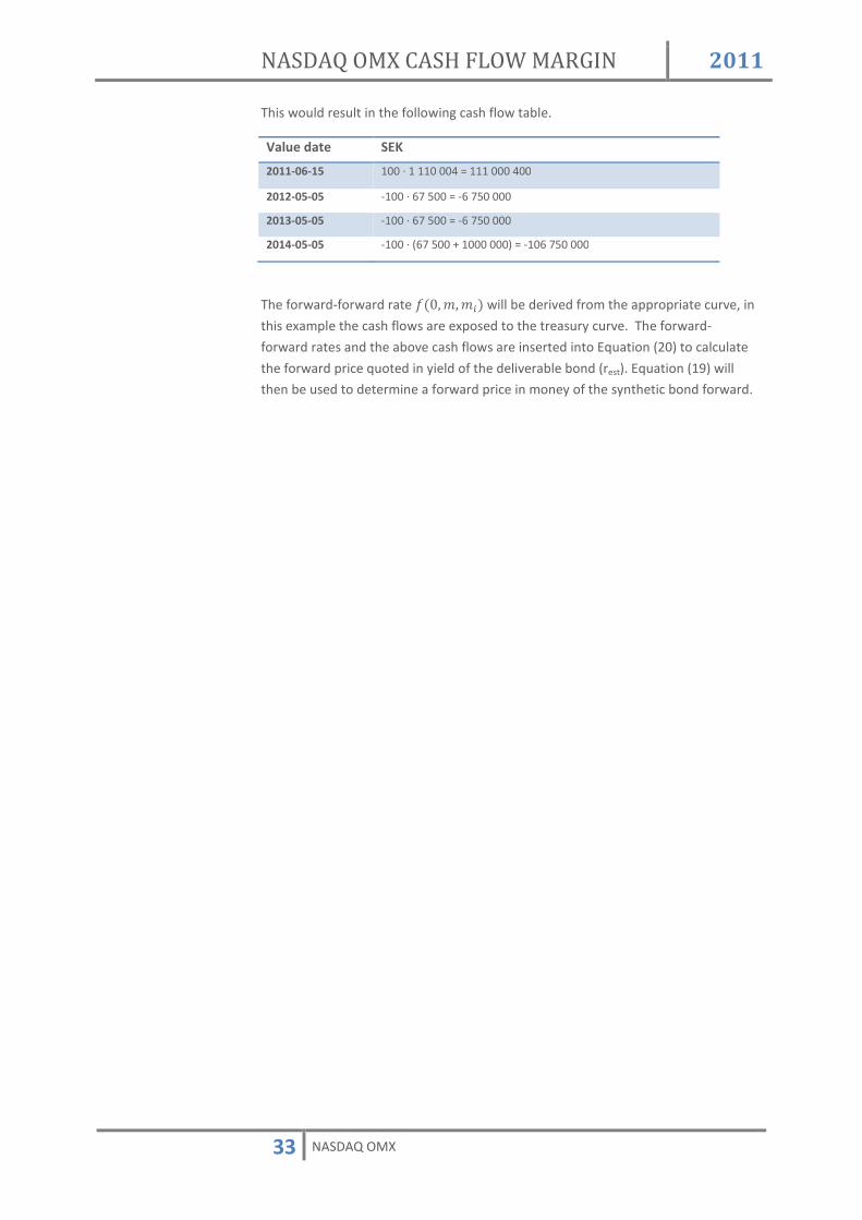
33 NASDAQ OMX
This would result in the following cash flow table.
Value date SEK
2011-06-15 100 · 1 110 004 = 111 000 400
2012-05-05 -100 · 67 500 = -6 750 000
2013-05-05 -100 · 67 500 = -6 750 000
2014-05-05 -100 · (67 500 + 1000 000) = -106 750 000
The forward-forward rate �������i� will be derived from the appropriate curve, in
this example the cash flows are exposed to the treasury curve. The forward-
forward rates and the above cash flows are inserted into Equation (20) to calculate
the forward price quoted in yield of the deliverable bond (rest). Equation (19) will
then be used to determine a forward price in money of the synthetic bond forward.

NASDAQ OMX CASH FLOW MARGIN 2011
34 NASDAQ OMX
OP T I O N S O N B O N D F O R W A R D S
The pricing of the Bond forward options builds on the same methodology used to
price the Bond forwards. The method for estimating the forward yield is exactly the
same. Given an estimated yield (rest), the calculation of the NPV for a specific option
is given by the following calculations.
DE F I N I T I O N S
Q = Quantity of underlying contracts N = Nominal contract size T = Time to expiry rS = Strike expressed as forward yield rest = Forward yield estimated from the curve σr = Yield volatility p = Value of option, expressed in yield BPV = Basis point value of underlying bond forward
F O R M U L A S
The strike yield, the estimated yield given by the curve, the yield volatility and the
time to expiry are entered into the Black 76 option pricing formula. If it is call
option, it is entered as a put, and vice versa. This reflects the inverse relation
between increases in price and yield. The result from Black 76 is the price of the
option expressed in yield. In order to convert this premium to a cash measure, the
BPV of the underlying bond forward is used.
z {��¼½lj���� ����� ��� �����������������������������������������������������������������������������������������29
��� {�� s z s � s ����������������������������������������������������������������������������������������������30

NASDAQ OMX CASH FLOW MARGIN 2011
35 NASDAQ OMX
MARGIN CALCULATIONS This section describes the margin calculations. The section starts with explaining
how each individual yield curve will be stressed, and correlation of different yield
curves is handled later on in the section.
NAK ED MA RGI N Once all OTC positions have been broken up into their future cash flows, then the
cash flow tables represent the total risk inherited from the positions in the account.
The account’s market value is obtained if these cash flows are discounted with the
official yield curves i.e. the market value is the position’s NPV. However, if the
shape of the yield curves changes the net present value of the cash flow tables will
also change. NOMX will simulate a number of different stressed yield curves and
recalculate the net present value of the cash flow tables using all these curves.
Figure: Schematic picture of the NPV calculations for SEK interest rate swaps.

NASDAQ OMX CASH FLOW MARGIN 2011
36 NASDAQ OMX
O B T A I N I N G T H E S E T O F S T R E S S E D C U R V E S
As describes in the “Yield curves” section of this document, NOMX will simulate
different curve changes using the curve’s principal components (PC).
A risk parameter will be defined per PC and the official spot curve will be stressed ±
its PC times that PC’s risk parameter. This process is described in more detail in the
“Yield curves” section in the beginning of the document and in the margin
calculation examples in the end of the document.
An updated version of the risk parameters can be found on:
http://nordic.nasdaqomxtrader.com/.
PE R F O R M I N G NPV C A L C U L A T I O N S
NOMX will calculate a net present value for each simulated spot curve. This involves
the following steps.
• Update the cash flow table’s exposed spot curve.
o Update the corresponding forward-forward curve.
o Update all floating cash flows in the cash flow table.
• Calculate the net present value of all floating and fixed cash flows in the
cash flow table using the recently updated spot curve

NASDAQ OMX CASH FLOW MARGIN 2011
37 NASDAQ OMX
COR R ELATIO N O F DI FFER EN T YI ELD CURV ES
Yield curves in the same currency but with different credit risks can show a historical
relationship. A currency’s treasury curve may be seen as the base curve, and the
other curves in the same currency can be obtained by applying a credit spread to
the treasury curve. NOMX applies the 3D window method in order to account for
correlation of different yield curves in the same currency.
The 3D window method might be difficult to digest for someone that is not used to
NOMX margin methodology. It is therefore recommended that Appendix III, that
describes the 1D window method, is read before this section.
S A M P L E S P A C E : S E T O F S T R E S S E D C U R V E S
NOMX simulates curve changes using the curve’s first three principal components.
The stressed curves therefore live in a three dimensional sample
spaceN;¾4� ;¾3� ;¾[P. All principal components will be stressed ± that PC’s risk parameter. This implies
that all possible curve changes are inside a rectangular prism. This rectangular prism
is called the vector cube.
NOMX divides the scanning range intervals N�;¾i , ;¾i¿@�7�@À�c878�>`>7� ;¾i ,;¾i¿@�7�@À�c878�>`>7P into a number of nodes, and the amount of ;¾i used in the
curve stressing will be evenly distributed over these nodes. Suppose, for example,
that the scanning range intervals of the three principal components are divided into
31, 5 and 3 nodes respectively. This would imply that there will be 31 · 5 · 3 = 465
nodes inside the vector cube, and each of these nodes would represent a stressed
spot curve.
Figure: All stressed curves are inside a vector cube.

NASDAQ OMX CASH FLOW MARGIN
38 NASDAQ OMX
C O R R E L A T I O N M E A S U R E D
Two yield curves that are 100% correlated cannot deviate from each other. This
implies that their stressing would
Figure: Example on two perfect correlated
However, two curves that are not 100%
When the first curve is stressed in one node
one of the
two curves may deviate from each other
by the correlation of the two curves.
the yield curves historical correlation
Figure: Example of two correlated curves.
PC1
The first princi
are two curves in the same
treasury curve and a mortgage curve.
30 basis points for t
would be extremely unlikely that
ASDAQ OMX CASH FLOW MARGIN
NASDAQ OMX
O R R E L A T I O N M E A S U R E D P E R P R I N C I P A L C O M P O N E N T S
Two yield curves that are 100% correlated cannot deviate from each other. This
implies that their stressing would have to be performed in the same nodes.
Example on two perfect correlated yield curves.
However, two curves that are not 100% correlated may deviate from each other.
When the first curve is stressed in one node, then the other curve may be within
one of the neighboring nodes. A volume determines the number of nodes that
curves may deviate from each other, and the size of this
by the correlation of the two curves. NOMX will determine this size by investigating
the yield curves historical correlation in each respective principal component.
Example of two correlated curves.
The first principal component is a parallel shift of the entire curve.
are two curves in the same currency but with different credit rating
treasury curve and a mortgage curve. Further suppose that PC1’s risk parameter is
30 basis points for the treasury curve and 33 basis points for the mortgage curve. It
would be extremely unlikely that the treasury curve experiences an upward parallel
2011
E N T S
Two yield curves that are 100% correlated cannot deviate from each other. This
performed in the same nodes.
correlated may deviate from each other.
the other curve may be within
determines the number of nodes that the
this volume is determined
NOMX will determine this size by investigating
in each respective principal component.
pal component is a parallel shift of the entire curve. Suppose there
currency but with different credit rating, for example a
PC1’s risk parameter is
basis points for the mortgage curve. It
the treasury curve experiences an upward parallel
NASDAQ OMX CASH FLOW MARGIN 2011
39 NASDAQ OMX
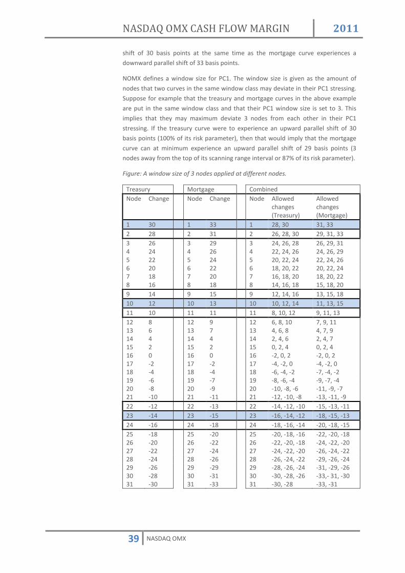
shift of 30 basis points at the same time as the mortgage curve experiences a
downward parallel shift of 33 basis points.
NOMX defines a window size for PC1. The window size is given as the amount of
nodes that two curves in the same window class may deviate in their PC1 stressing.
Suppose for example that the treasury and mortgage curves in the above example
are put in the same window class and that their PC1 window size is set to 3. This
implies that they may maximum deviate 3 nodes from each other in their PC1
stressing. If the treasury curve were to experience an upward parallel shift of 30
basis points (100% of its risk parameter), then that would imply that the mortgage
curve can at minimum experience an upward parallel shift of 29 basis points (3
nodes away from the top of its scanning range interval or 87% of its risk parameter).
Figure: A window size of 3 nodes applied at different nodes.
Treasury Mortgage Combined Node Change Node Change Node Allowed
changes (Treasury)
Allowed changes (Mortgage)
1 30 1 33 1 28, 30 31, 33 2 28 2 31 2 26, 28, 30 29, 31, 33 3 26 3 29 3 24, 26, 28 26, 29, 31 4 24 4 26 4 22, 24, 26 24, 26, 29 5 22 5 24 5 20, 22, 24 22, 24, 26 6 20 6 22 6 18, 20, 22 20, 22, 24 7 18 7 20 7 16, 18, 20 18, 20, 22 8 16 8 18 8 14, 16, 18 15, 18, 20 9 14 9 15 9 12, 14, 16 13, 15, 18 10 12 10 13 10 10, 12, 14 11, 13, 15 11 10 11 11 11 8, 10, 12 9, 11, 13 12 8 12 9 12 6, 8, 10 7, 9, 11 13 6 13 7 13 4, 6, 8 4, 7, 9 14 4 14 4 14 2, 4, 6 2, 4, 7 15 2 15 2 15 0, 2, 4 0, 2, 4 16 0 16 0 16 -2, 0, 2 -2, 0, 2 17 -2 17 -2 17 -4, -2, 0 -4, -2, 0 18 -4 18 -4 18 -6, -4, -2 -7, -4, -2 19 -6 19 -7 19 -8, -6, -4 -9, -7, -4 20 -8 20 -9 20 -10, -8, -6 -11, -9, -7 21 -10 21 -11 21 -12, -10, -8 -13, -11, -9 22 -12 22 -13 22 -14, -12, -10 -15, -13, -11 23 -14 23 -15 23 -16, -14, -12 -18, -15, -13 24 -16 24 -18 24 -18, -16, -14 -20, -18, -15 25 -18 25 -20 25 -20, -18, -16 -22, -20, -18 26 -20 26 -22 26 -22, -20, -18 -24, -22, -20 27 -22 27 -24 27 -24, -22, -20 -26, -24, -22 28 -24 28 -26 28 -26, -24, -22 -29, -26, -24 29 -26 29 -29 29 -28, -26, -24 -31, -29, -26 30 -28 30 -31 30 -30, -28, -26 -33,- 31, -30 31 -30 31 -33 31 -30, -28 -33, -31

NASDAQ OMX CASH FLOW MARGIN 2011
40 NASDAQ OMX
• A window of 3 nodes applied at node 1 implies that if the treasury curve
experiences an upward shift of 28 or 30 basis points, then the mortgage
curve may experience an upward shift of 31 or 33 basis points.
• A window of 3 nodes applied at node 10 implies that if the treasury curve
experiences an upward shift of 10, 12 or 14 basis points, then the mortgage
curve may experience an upward shift of 11, 13 or 15 basis points.
• A window of 3 nodes applied at node 23 implies that if the treasury curve
experiences a downward shift of 12, 14 or 16 basis points, then the
mortgage curve may experience a downward shift of 13, 15 or 18 basis
points.
PC2
The second principal component is a change in the curve’s slope. NOMX will also
define a window size for this principal component. This window size determines the
maximum amount of nodes that two curves in the same window class may deviate
from each other in terms of their PC2 stressing.
PC3
The third principal component is a change in the curve’s curvature. NOMX will also
define a window size for this principal component. This window size determines the
maximum amount of nodes that two curves in the same window class may deviate
from each other in terms of their PC3 stressing.
W I N D O W C U B E S
The window sizes for each principal component constitute a rectangular prism (the
window cube) in the N;¾4� ;¾3� ;¾[P space. This prism determines the number of
nodes that the curves in the same window class may deviate from each other.
3D W I N D O W M E T H O D
The 3D window method starts by listing all vector cubes in the same window class
next to each other.
• A result vector cube is created and placed next to the other vector cubes.
• A window cube is placed in every top node of the vector cubes.
o The result vector’s value at node i is the sum of each vector cube’s
lowest net present value from the nodes inside the window cube
that is placed at node i.
• The window cubes will slide down all nodes in the vector cubes and the
value in the result vector cube will always be the sum of the lowest net
present values from the nodes inside the window cubes.

NASDAQ OMX CASH FLOW MARGIN 2011
41 NASDAQ OMX
Figure: 3D window method applied on the treasury and mortgage vector cubes.
W I N D O W T R E E S
The window tree is built up of several layers of window classes and the curves with
the closest correlation are placed in the same window class in the bottom of the
tree.
The window method is a recursive method; it is first applied to the window classes
in the bottom of the window tree. It is here applied on the vector cubes of the cash
flow tables within the same window class. During this process a new vector cube,
the result vector cube, is created according to the procedures described above. The
result vector cube is then combined with result vector cubes from the other window
classes in the tree and, as a result, a new result vector cube is created. This
procedure is repeated until the top of the window tree has been reached.
Figure: example of a possible SEK window tree

NASDAQ OMX CASH FLOW MARGIN 2011
42 NASDAQ OMX
MARGIN CALCULATION EXAMPLES This section presents a few examples on margin calculations.
EXAMPLE 1 REPO T RA NS A CTION W ITH TWO OP EN LEGS
PO S I T I O N S
Considerer a one week REPO in RGKB1045.
Standard = Buy and sell back. t = 2009-11-02. ts = 2009-11-04. te = 2009-11-11. tm = 2011-03-15. tc = 2009-03-15. Q = 1 000. N = SEK 1 000 000. C = 5,25. Side = 1. CP = 105,89. rrepo = 0,35%. Ci = Payment 52 500 1 052 500
Date 2010-03-15 2011-03-15
C A S H F L O W T A B L E S
ST A R T C O N S I D E R A T I O N
Equation (4) is used to calculate the start consideration. It is 229 days between
2009-03-15 and 2009-11-04 in a 30E convention.
QR �4�2�ST * 2�32 , UUV��W� , X�WWW�WWWXWW , 4��� Y:Z�4��T3�3T2�S[[
E N D C O N S I D E R A T I O N
Equation (6) is used to calculate the end consideration.
Q\ 4��T3�3T2�S[[ , �4 * ��[2] , ^��W� Y:Z�4��T3�[l��4l�
This results in the following two cash flow tables.
ST A R T A N D E N D C O N S I D E R A T I O N C A S H F L O W T A B L E (S W A P C U R V E )
Equations (8) – (9) are used to insert the start and end considerations into the start
and end consideration cash flow table.
Value date Time to maturity SEK 2009-11-04 0,0056 1 092 295 833 2009-11-11 0,025 -1 092 370 170

NASDAQ OMX CASH FLOW MARGIN 2011
43 NASDAQ OMX
TR E A S U R Y C A S H F L O W T A B L E
Before the start date of the REPO, the underlying bonds have not been exchanged,
and since the underlying bonds do not pay any coupons in the interval [ts+5, te+5]
the cash flows from Equation (11) and Equation (12) will cancel each other out. This
implies that the treasury cash flow table will be empty until after the start date of
the REPO.
C U R V E S T R E S S I N G
This position is exposed to a shift in the SEK Treasury spot curve and it is this curve
that will be stressed in the margin calculation.
R I S K P A R A M E T E R S
The shape of the SEK Treasury curve’s principal components is shown in the figure
below.
Figure: Shape of the SEK Treasury curve’s principal components.
The tables below list the stress levels together with the first points of the principal
components for the SEK Treasury curve.
ST R E S S L E V E L S
Curve PC1 PC2 PC3 Treasury 22 basis points 8 basis points 5 basis points
PR I N C I P A L C O M P O N E N T S
Time to maturity PC1 PC2 PC3 0 1 1 1 0,25 1 0,8 0,64
-0.6
-0.4
-0.2
0
0.2
0.4
0.6
0.8
1
1.2
00.
5 11.
5 22.
5 33.
5 44.
5 55.
5 66.
5 77.
5 88.
5 99.
5 10PC1 PC2 PC3

NASDAQ OMX CASH FLOW MARGIN 2011
44 NASDAQ OMX
OF F I C I A L C U R V E S
NOMX will, on each trading day, bootstrap official yield curves that will be used to
price all cleared instruments. It is the official yield curves that will be stressed in the
margin calculations. In this example it is assumed that the official SEK Treasury
curve looks as in the figure below.
Figure: Treasury curve
The table below lists the official Treasury spot rates for the time to maturities that
are relevant to the cash flows in the start and end consideration cash flow table.
Time to maturity Spot rate 0,0056 ��[24]
0,025 ��[2_]
ST R E S S E D C U R V E S
The worst outcome for the position is that the two day SEK Treasury spot rate goes
up while the one week SEK Treasury spot rate goes down. This is, however, not a
realistic scenario. NOMX will simulate stressed curves with the three principal
components and the margin requirement will be based on the worst of these
stressed curves.
A cash flow that is due in a long time is more exposed to a shift in the yield curve
compared to a cash flow that is due soon. In this example there are only two cash
flows and the largest cash flow is the one that has longest time to maturity. This is a
negative cash flow (SEK -1 092 370 170) and the worst outcome is therefore that the
SEK Treasury curve drops. The worst outcome will be the scenario where all three
principal components are stressed downwards.
0.00%
0.50%
1.00%
1.50%
2.00%
2.50%
3.00%
3.50%
4.00%
4.50%
00.
5 11.
5 22.
5 33.
5 44.
5 55.
5 66.
5 77.
5 88.
5 99.
5 10

NASDAQ OMX CASH FLOW MARGIN 2011
45 NASDAQ OMX
Figure: All three principal components will be stressed downwards in the worst
scenario.
Figure: Official SEK Treasury curve and stressed SEK Treasury curve
NOMX defines the principal components in a predefined number of nodes. The
distance between each node is in this example 0,25 years. It is, however, 0,0056
years to the start date of the REPO and 0,025 years to the end date of the REPO. A
linear interpolation will be used in order to determine the stress levels for these
maturities. This can be seen in the table below.
Time to maturity
PC1 PC2 PC3
0 1 1 1
0,0056 1 4 * ��S � 4��32 � � , �����2j� �� ��TT223
4 * ��j_ � 4��32 � � , �����2j� �� ��TT4T[j
0,025 1 4 * ��S � 4��32 � � , ����32 � �� ��TS 4 * ��j_ � 4��32 � � , ����32 � �� ��Tj_
0,25 1 0,8 0,64
-0.40%
-0.35%
-0.30%
-0.25%
-0.20%
-0.15%
-0.10%
-0.05%
0.00%
0.05%
00.
5 11.
5 22.
5 33.
5 44.
5 55.
5 66.
5 77.
5 88.
5 99.
5 10
Combined stressing PC1 PC2 PC3
0.00%
0.50%
1.00%
1.50%
2.00%
2.50%
3.00%
3.50%
4.00%
4.50%
00.
5 11.
5 22.
5 33.
5 44.
5 55.
5 66.
5 77.
5 88.
5 99.
5 10

NASDAQ OMX CASH FLOW MARGIN 2011
46 NASDAQ OMX
The table below shows the stressed Treasury spot rates when the three principal
components are stressed downwards.
Time to maturity
Spot rate Stressed spot rate
0,0056 0,351% ��[24] � ��33] , 4 � ���S] , ��TT223 � ���2] , ��TT4T[j ����4lj3]
0,025 0,354% ��[2_] � ��33] , 4 � ���S] , ��TS � ���2] , ��Tj_ ����l_]
NE T P R E S E N T V A L U E
The margin requirement is obtained by calculating the net present value of the cash
flows in all cash flow tables.
In this example all cash flows are in SEK and are exposed to the Treasury curve. If
the net present value is calculated with the official SEK Treasury curve, then the
REPO position’s market value is obtained. If, on the other hand, the net present
value is calculated with the stressed SEK Treasury curve, then the REPO position’s
margin requirement is obtained.
Value date Time to maturity
SEK
2009-11-04 0,0056 1 092 295 833
2009-11-11 0,025 -1 092 370 170
NPV 4��T3�3T2�S[[�4 * ��[24]�W�WW�� � 4��T3�[l��4l��4 * ��[2_]�W�WU� l[�
NPV stressed 4��T3�3T2�S[[�4 * ����4lj3]�W�WW�� � 4��T3�[l��4l��4 * ����l_]�W�WU� �l3�_3_
Market value = SEK 730
It can be noted that NOMX gives the REPO position a market value that is not zero
even though the position was just entered. This is because the NPV are calculated
from a yield curve (a constructed average) and the repo rates are actual agreed
transfer rates between parties.
Margin requirement = SEK -72 424

NASDAQ OMX CASH FLOW MARGIN 2011
47 NASDAQ OMX
EXAMPLE 2 REPO T RA NS A CTION W ITH ON E OP EN LEG
PO S I T I O N S
This example contains the same position as in Example 1, i.e. a one week REPO in
RGKB1045. However, this example describes the margin calculations performed at
2009-11-04 when the first leg has settled.
ST A R T A N D E N D C O N S I D E R A T I O N C A S H F L O W T A B L E
The first leg has settled so it is only the end consideration that is left in the start and
end consideration cash flow table.
Value date Time to maturity SEK 2009-11-11 0,1944 -1 092 370 170
TR E A S U R Y C A S H F L O W T A B L E
Equation (12) is used to insert the cash flows from the underlying bond, which is to
be exchanged on the end date, into the treasury cash flow table.
Value date Time to maturity SEK 2010-03-15 0,3639 4���� , 23�2�� 23�2������ 2011-03-15 1,3639 4���� , 4��23�2�� 4��23�2������
C U R V E S T R E S S I N G
This position is exposed to shifts in the SEK Treasury spot curve
R I S K P A R A M E T E R S
The tables below list the stress levels together with the first points of the principal
components.
ST R E S S L E V E L S
Curve PC1 PC2 PC3 Treasury 22 basis points 8 basis points 5 basis points
PR I N C I P A L C O M P O N E N T S
Time to maturity PC1 PC2 PC3 0 1 1 1 0,25 1 0,8 0,64 0,5 1 0,6 0,27 0,75 1 0,49 0,02 1 1 0,41 -0,16 1,25 1 0,34 -0,27 1,5 1 0,29 -0,33
OF F I C I A L C U R V E S
NOMX will, on each trading day, bootstrap official yield curves that will be used to
price all cleared instruments. It is the official yield curves that will be stressed in the
margin calculations. In this example it is assumed that the official SEK treasury curve
look as in the figure below.

NASDAQ OMX CASH FLOW MARGIN 2011
48 NASDAQ OMX
Figure: Treasury curve
The tables below list the treasury spot rates for the time to maturities that are
relevant to the cash flows in the start and end consideration cash flow table and in
the treasury cash flow table.
SE K TR E A S U R Y
Time to maturity Spot rate 0,01944 ��[23]
0,3639 ��_�]
1,3639 4�42]
0.00%
0.50%
1.00%
1.50%
2.00%
2.50%
3.00%
3.50%
4.00%
4.50%
00.
5 11.
5 22.
5 33.
5 44.
5 55.
5 66.
5 77.
5 88.
5 99.
5 10

NASDAQ OMX CASH FLOW MARGIN 2011
49 NASDAQ OMX
ST R E S S E D C U R V E S
The first cash flow is a negative one and thus the worst scenario for that cash flow
will be that all short SEK treasury spot rates goes down. However, the position’s
cash flows that are most distance are the ones that are derived from the underlying
bond. These are all positive cash flows and hence these positions are mainly
exposed to an upward shift in the SEK treasury curve; especially that the interest
rate with maturity 1,3639 years goes up. If one considers all cash flows, the worst
outcome will be the scenario where the first two principal components are stressed
upwards and the third principal component is stressed downwards.
Figure: The worst scenario is when the SEK treasury curve is stressed upward.
Figure: Official curve and stressed curve.
NOMX defines the principal components in a predefined number of nodes. The
distance between each node is in this example 0,25 years. A linear interpolation will
be used in order to determine the stress levels for the maturities that lay in
between these nodes. This can be seen in the table below.
-0.10%
0.00%
0.10%
0.20%
0.30%0
0.5 1
1.5 2
2.5 3
3.5 4
4.5 5
5.5 6
6.5 7
7.5 8
8.5 9
9.5 10
PC1 (treasury) PC2 (treasury)
PC3 (treasury) Combined stressing (treasury)
0.00%
0.50%
1.00%
1.50%
2.00%
2.50%
3.00%
3.50%
4.00%
4.50%
00.
5 11.
5 22.
5 33.
5 44.
5 55.
5 66.
5 77.
5 88.
5 99.
5 10

NASDAQ OMX CASH FLOW MARGIN 2011
50 NASDAQ OMX
Time to maturity
PC1 PC2 PC3
0 1 1 1
0,01944 1 4 * ��S � 4��32 � � , �����4T__ � �� ��TS__ 4 * ��j_ � 4��32 � � , ����4T__ � �� ��Tl3�
0,25 1 0,8 0,64
0,3639 1 ��S * ��j � ��S��2 � ��32 , ���[j[T� ��32� ��l�ST
��j_ * ��3l � ��j_��2 � ��32 , ���[j[T� ��32� ��_l4_
0,5 1 0,6 0,27 0,75 1 0,49 0,02 1 1 0,41 -0,16 1,25 1 0,34 -0,27
1,3639 1 ��[_ * ��3T � ��[_4�2 � 4�32 , �4�[2ST� 4�32� ��[4l3
���3l * ���[[ * ��3l4�2 � 4�32 , �4�[j[T� 4�32� ���3Tl[
1,5 1 0,29 -0,33
SE K T R E A S U R Y
The table below shows the stressed treasury spot rates when the first two principal
components are stressed upwards and the third principal component is stressed
downwards.
Time to maturity
Spot rate
Stressed spot rate
0,01944 0,352% ��[23] * ��33] , 4 * ���S] , ��TS__ � ���2] , ��Tl3� ��j�33]
0,3639 0,40% ��_�] * ��33] , 4 * ���S] , ��l�ST � ���2] , ��_l4_ ��j2[4]
1,3639 1,15% 4�42] * ��33] , 4 * ���S] , ��[4l3 * ���2] , ��3Tl[ 4�_4�3]

NASDAQ OMX CASH FLOW MARGIN 2011
51 NASDAQ OMX
NE T P R E S E N T V A L U E
The margin requirement is obtained by calculating the net present value of the cash
flows in the cash flow table.
If the net present value is calculated with the official SEK treasury curve, then the
position’s market value is obtained. If, on the other hand, the net present value is
calculated with the stressed treasury curve, then the position’s margin requirement
is obtained.
ST A R T A N D E N D C O N S I D E R A T I O N C A S H F L O W T A B L E
Value date Time to maturity
SEK
2009-11-11 0,01944 -1 092 370 170
NPV (B&�
� 4��T3�[l��4l��4 * ��[23]�W�WXVkk � �4��T3�3Tj�22_
NPV stressed �ÁÂ�
� 4��T3�[l��4l��4 * ��j�33]�W�WXVkk �4��T3�3_3�jS�
C A S H F L O W T A B L E D E R I V E D F R O M T H E U N D E R L Y I N G B O N D
Value date Time to maturity
SEK
2010-03-15 0,3639 52 500 000 2011-03-15 1,3639 1 052 500 000
NPV 23�2�������4 * ��_�]�W����V * 4��23�2�������4 * 4�42]�X����V 4��SS�j[l��4_
NPV stressed
23�2�������4 * ��j2[4]�W����V * 4��23�2�������4 * 4�_4�3]�X����V 4��S_�Tj_�_2[
Market value = SEK 1 088 637 014 – SEK 1 092 296 554 = SEK -3 659 540
Margin requirement = SEK 1 084 964 453 – SEK 1 092 242 680 = SEK -7 278 227

NASDAQ OMX CASH FLOW MARGIN 2011
52 NASDAQ OMX
EXAMPLE 3 SPR EA D PO SITION IN A REPO T RA NS A CTION
PO S I T I O N S
Considerer a one week REPO in RGKB1049 versus a one week reversed REPO in
RGKB1050. These positions are traded on 2009-11-02, but the margin calculation
presented here is performed on 2009-11-04 after their first legs have settled.
ON E W E E K R E P O I N RGKB1049
Standard = Buy and sell back. t = 2009-11-04. ts = 2009-11-04. te = 2009-11-11. tm = 2015-08-12. tc = 2009-08-12. Q = 1 000. N = SEK 1 000 000. C = 4,5. Side = 1. CP = 108,94 rrepo = 0,35%. Ci = Payment 45 000 … 45 000 1 045 000
Date 2010-08-12 … 2014-08-12 2015-08-12
ON E W E E K R E V E R S E D R E P O I N RGKB 1050
Standard = Buy and sell back. t = 2009-11-04. ts = 2009-11-04. te = 2009-11-11. tm = 2016-07-12. tc = 2009-07-12. Q = 1 000. N = SEK 1 000 000. C = 3. Side = -1. CP = 98,50. rrepo = 0,35%. Ci = Payment 30 000 … 30 000 1 030 000
Date 2010-07-12 … 2015-07-12 2016-07-12
C A S H F L O W T A B L E S
ST A R T C O N S I D E R A T I O N
R G K B1049
Equation (4) is used to calculate the start consideration. It is 82 days between 2009-
08-12 and 2009-11-04 in a 30E convention.
QR �4�S�T_ * _�2 , mU��W� , X�WWW�WWWXWW , 4��� Y:Z�4��TT�j2�����
R G K B1050

NASDAQ OMX CASH FLOW MARGIN 2011
53 NASDAQ OMX
Equation (4) is used to calculate the start consideration. It is 112 days between
2009-07-12 and 2009-11-04 in a 30E convention.
QR �TS�2� * [ , XXU��W� , X�WWW�WWWXWW , 4��� Y:Z�TT_�[[[�[[[
E N D C O N S I D E R A T I O N
R G K B1049
Equation (6) is used to calculate the end consideration.
Q\ 4��TT�j2����� , �4 * ��[2] , ^��W� Y:Z�4��TT�l3_�S[l
R G K B1050
Equation (6) is used to calculate the end consideration.
Q\ TT_�[[[�[[[ , �4 * ��[2] , ^��W� Y:Z�TT_�_�4���[
This results in the following two cash flow tables.
ST A R T A N D E N D C O N S I D E R A T I O N C A S H F L O W T A B L E
The first leg has settled so it is only the end considerations that remain in the start
and end consideration cash flow table. These have been entered using Equation (9).
Value date Time to maturity SEK 2009-11-11 0,01944 -1 099 724 837 + 994 401 003 = -105 323 834
C A S H F L O W T A B L E D E R I V E D F R O M T H E U N D E R L Y I N G B O N D S
Equation (12) is used to insert the cash flows from the underlying bonds, which are
to be exchanged on the end date, into the treasury cash flow table.
Value date Time to maturity SEK 2010-07-12 0,6889 �4���� , [����� �[��������� 2010-08-12 0,7722 4���� , _2���� _2�������� 2011-07-12 1,6889 �4���� , [����� �[��������� 2011-08-12 1,7722 4���� , _2���� _2�������� 2012-07-12 2,6889 �4���� , [����� �[��������� 2012-08-12 2,7722 4���� , _2���� _2�������� 2013-07-12 3,6889 �4���� , [����� �[��������� 2013-08-12 3,7722 4���� , _2���� _2�������� 2014-07-12 4,6889 �4���� , [����� �[��������� 2014-08-12 4,7722 4���� , _2���� _2�������� 2015-07-12 5,6889 �4���� , [����� �[��������� 2015-08-12 5,7722 4���� , 4��_2���� 4��_2�������� 2016-07-12 6,6889 �4���� , 4��[����� �4��[���������
C U R V E S T R E S S I N G

NASDAQ OMX CASH FLOW MARGIN 2011
54 NASDAQ OMX
This combined position is exposed to shifts in the SEK treasury spot curve. The
treasury curve will be stressed in the margin calculation.
R I S K P A R A M E T E R S
The tables below list the stress levels together with the first points on the principal
components.
ST R E S S L E V E L S
Curve PC1 PC2 PC3 Treasury 22 basis points 8 basis points 5 basis points
PR I N C I P A L C O M P O N E N T S
Time to maturity PC1 PC2 PC3 0 1 1 1 0,25 1 0,8 0,64 0,5 1 0,6 0,27 0,75 1 0,49 0,02 1 1 0,41 -0,16 1,25 1 0,34 -0,27 1,5 1 0,29 -0,33 1,75 1 0,25 -0,35 2 1 0,21 -0,35 2,25 1 0,18 -0,32 2,5 1 0,15 -0,29 2,75 1 0,12 -0,25 3 1 0,09 -0,21 3,25 1 0,07 -0,16 3,5 1 0,05 -0,12 3,75 1 0,03 -0,09 4 1 0,01 -0,06 4,25 1 -0,01 -0,03 4,5 1 -0,02 -0,01 4,75 1 -0,04 0,01 5 1 -0,05 0,02 5,25 1 -0,07 0,03 5,5 1 -0,08 0,04 5,75 1 -0,09 0,05 6 1 -0,1 0,06 6,25 1 -0,12 0,06 6,5 1 -0,13 0,07 6,75 1 -0,14 0,08

NASDAQ OMX CASH FLOW MARGIN 2011
55 NASDAQ OMX
OF F I C I A L C U R V E S
NOMX will, on each trading day, bootstrap official yield curves that will be used to
price all cleared instruments. It is the official yield curves that will be stressed in the
margin calculations. In this example it is assumed that the official SEK treasury curve
look as in the figure below.
Figure: Official SEK treasury curve
The tables below list the official treasury spot rates for the time to maturities that
are relevant to the cash flows in the start and end consideration cash flow table and
in the treasury cash flow table.
SE K T R E A S U R Y
Time to maturity
Spot rate
0,01944 ��[23] 0,6889 ��j3] 0,7722 ��ST% 1,6889 4�__] 1,7722 4�Sl% 2,6889 3�3T] 2,7722 3�2l% 3,6889 3�Sj] 3,7722 [��[% 4,6889 [�4T] 4,7722 [�[�% 5,6889 [�_4] 5,7722 [�_T% 6,6889 [�2S]
ST R E S S E D C U R V E S
This combined position is mainly exposed to a downward shift in the SEK treasury
curve. The worst outcome for the SEK treasury curve will therefore be a downward
stressing combined with a change in slope. This is the scenario where the first and
0.00%
0.50%
1.00%
1.50%
2.00%
2.50%
3.00%
3.50%
4.00%
4.50%
00.
5 11.
5 22.
5 33.
5 44.
5 55.
5 66.
5 77.
5 88.
5 99.
5 10

NASDAQ OMX CASH FLOW MARGIN 2011
56 NASDAQ OMX
the third principal components are stressed downwards and the second principal
component is stressed upwards.
Figure: The worst scenario is when the SEK treasury curve is stressed downwards.
Figure: Official curves and stressed curves.
NOMX defines the principal components in a predefined number of nodes. The
distance between each node is in this example 0,25 years. A linear interpolation will
be used in order to determine the stress levels for the maturities that lay in
between these nodes. This can be seen in the table below.
-0.25%
-0.20%
-0.15%
-0.10%
-0.05%
0.00%
0.05%
0.10%
00.
5 11.
5 22.
5 33.
5 44.
5 55.
5 66.
5 77.
5 88.
5 99.
5 10
PC1 (treasury) PC2 (treasury)
PC3 (treasury) Combined stressing (treasury)
0.00%
0.50%
1.00%
1.50%
2.00%
2.50%
3.00%
3.50%
4.00%
4.50%
00.
5 11.
5 22.
5 33.
5 44.
5 55.
5 66.
5 77.
5 88.
5 99.
5 10
Official SEK swap curve Stressed SEK swap curve

NASDAQ OMX CASH FLOW MARGIN 2011
57 NASDAQ OMX
Time to maturity
PC1 PC2 PC3
0 1 1 1
0,01944 1 4 * ��S � 4��32 � � , ����4T__ � �� ��TS__ 4 * ��j_ � 4��32 � � , ����4T__ � �� ��Tl3�
0,25 1 0,8 0,64 0,5 1 0,6 0,27
0,6889 1 ��j * ��_T � ��j��l2 � ��2 , ���jSST� ��2� ��24jT
��3l * ���3 � ��3l��l2 � ��2 , ���jSST� ��2� ���S44
0,75 1 0,49 0,02
0,7722 1 ��_T * ��_4 � ��_T4 � ��l2 , ���ll33� ��l2� ��_S3T
���3 * ���4j � ���34 � ��l2 , ���ll33 � ��l2� ����_� 1 1 0,41 -0,16 1,25 1 0,34 -0,27 1,5 1 0,29 -0,33
1,6889 1 ��3T * ��32 � ��3T4�l2 � 4�2 , �4�jSST� 4�2� ��32TS
���[[ * W��� W���X�^�X�� , �4�jSST� 4�2� ���[_21
1,75 1 0,25 -0,35
1,7722 1 ��32 * ��34 � ��323 � 4�l2 , �4�ll33� 4�l2� ��3_j_
���[2 * ���[2 * ��[23 � 4�l2 , �4�ll33 � 4�l2� ���[2 2 1 0,21 -0,35 2,25 1 0,18 -0,32 2,5 1 0,15 -0,29
2,6889 1 ��42 * ��43 � ��423�l2 � 3�2 , �3�jSST� 3�2� ��43l[
���3T * ���32 * ��3T3�l2 � 3�2 , �3�jSST � 3�2� ���32TS 2,75 1 0,12 -0,25
2,7722 1 ��43 * ���T � ��43[ � 3�l2 , �3�ll33� 3�l2� ��44l[
���32 * ���34 * ��32[ � 3�l2 , �3�ll33 � 3�l2� ���3_j_ 3 1 0,09 -0,21 3,25 1 0,07 -0,16 3,5 1 0,05 -0,12
3,6889 1 ���2 * ���[ � ���2[�l2 � [�2 , �[�jSST � [�2� ���[_T
���43 * ����T * ��43[�l2 � [�2 , �[�jSST � [�2� ����Tl[ 3,75 1 0,03 -0,09
3,7722 1 ���[ * ���4 � ���[_ � [�l2 , �[�ll33� [�l2� ���3S3
����T * ����j * ���T_ � [�l2 , �[�ll33 � [�l2� ����Sl[ 4 1 0,01 -0,06 4,25 1 -0,01 -0,03 4,5 1 -0,02 -0,01
4,6889 1 ����3 * ����_ * ���3_�l2 � _�2 , �_�jSST� _�2� ����[24
����4 * ���4 * ���4_�l2 � _�2 , �_�jSST � _�2� ����24
4,75 1 -0,04 0,01
4,7722 1
����_ * ����2 * ���_2 � _�l2 , �_�ll33� _�l2� ����_�T
���4 * ���3 � ���42 � _�l2 , �_�ll33� _�l2� ���4�T
5 1 -0,05 0,02 5,25 1 -0,07 0,03 5,5 1 -0,08 0,04

NASDAQ OMX CASH FLOW MARGIN 2011
58 NASDAQ OMX
5,6889 1 ����S * ����T * ���S2�l2 � 2�2 , �2�jSST� 2�2� ����Slj
���_ * ���2 � ���_2�l2 � 2�2 , �2�jSST� 2�2� ���_lj
5,75 1 -0,09 0,05
5,7722 1 ����T * ���4 * ���Tj � 2�l2 , �2�ll33� 2�l2� ����T�T
���2 * ���j � ���2j � 2�l2 , �2�ll33� 2�l2� ���2�T
6 1 -0,1 0,06 6,25 1 -0,12 0,06 6,5 1 -0,13 0,07
6,6889 1 ���4[ * ���4_ * ��4[j�l2 � j�2 , �j�jT � j�2� ���4[lj
���l * ���S � ���lj�l2 � j�2 , �j�jSST� j�2� ���llj
6,75 1 -0,14 0,08
SE K T R E A S U R Y
The table below shows the stressed treasury spot rates when the first and the third
principal components are stressed downwards and the second principal component
is stressed upwards.
Time to maturity
Spot rate
Spot rate stressed
0,01944 0,352% ��[23] � ��33] , 4 * ���S] , ��TS__ � ���2] , ��Tl3� ��4j3]
0,6889 0,62% ��j3] � ��33] , 4 * ���S] , ��24jT � ���2] , ���S44 ��_[l]
0,7722 0,89% ��ST] � ��33] , 4 * ���S] , ��_S3T � ���2] , ����_� ��l�S]
1,6889 1,44% 4�__] � ��33] , 4 * ���S] , ��32TS * ���2] , ��[_24 4�32S]
1,7722 1,87% 4�Sl] � ��33] , 4 * ���S] , ��3_j_ * ���2] , ��[2 4�jSl]
2,6889 2,29% 3�3T] � ��33] , 4 * ���S] , ��43l[ * ���2] , ��32TS 3��T[]
2,7722 2,57% 3�2l] � ��33] , 4 * ���S] , ��44l[ * ���2] , ��3_j_ 3�[l3]
3,6889 2,86% 3�Sj] � ��33] , 4 * ���S] , ���[_T * ���2] , ���Tl[ 3�j_S]
3,7722 3,03% [��[] � ��33] , 4 * ���S] , ���3S3 * ���2] , ���Sl[ 3�S4l]
4,6889 3,19% [�4T] � ��33] , 4 � ���S] , ���[24 � ���2] , ����24 3�Tjl]
4,7722 3,30% [�[�] � ��33] , 4 � ���S] , ���_�T � ���2] , ���4�T [��lj]
5,6889 3,41% [�_4] � ��33] , 4 � ���S] , ���Slj � ���2] , ���_lj [�4S4]
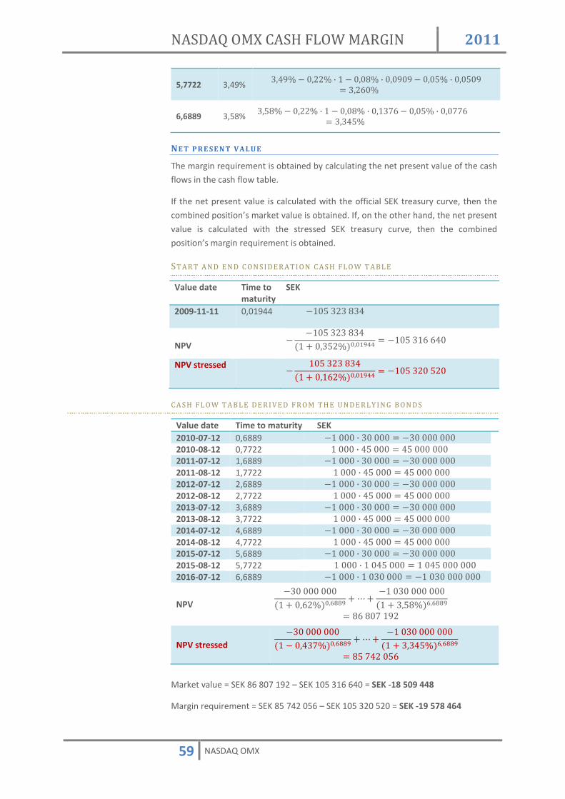
NASDAQ OMX CASH FLOW MARGIN 2011
59 NASDAQ OMX
5,7722 3,49% [�_T] � ��33] , 4 � ���S] , ���T�T � ���2] , ���2�T [�3j�]
6,6889 3,58% [�2S] � ��33] , 4 � ���S] , ��4[lj � ���2] , ���llj [�[_2]
NE T P R E S E N T V A L U E
The margin requirement is obtained by calculating the net present value of the cash
flows in the cash flow table.
If the net present value is calculated with the official SEK treasury curve, then the
combined position’s market value is obtained. If, on the other hand, the net present
value is calculated with the stressed SEK treasury curve, then the combined
position’s margin requirement is obtained.
ST A R T A N D E N D C O N S I D E R A T I O N C A S H F L O W T A B L E
Value date Time to maturity
SEK
2009-11-11 0,01944 �4�2�[3[�S[_
NPV
� �4�2�[3[�S[_�4 * ��[23]�W�WXVkk �4�2�[4j�j_�
NPV stressed � 4�2�[3[�S[_�4 * ��4j3]�W�WXVkk �4�2�[3��23�
C A S H F L O W T A B L E D E R I V E D F R O M T H E U N D E R L Y I N G B O N D S
Value date Time to maturity SEK 2010-07-12 0,6889 �4���� , [����� �[��������� 2010-08-12 0,7722 4���� , _2���� _2�������� 2011-07-12 1,6889 �4���� , [����� �[��������� 2011-08-12 1,7722 4���� , _2���� _2�������� 2012-07-12 2,6889 �4���� , [����� �[��������� 2012-08-12 2,7722 4���� , _2���� _2�������� 2013-07-12 3,6889 �4���� , [����� �[��������� 2013-08-12 3,7722 4���� , _2���� _2�������� 2014-07-12 4,6889 �4���� , [����� �[��������� 2014-08-12 4,7722 4���� , _2���� _2�������� 2015-07-12 5,6889 �4���� , [����� �[��������� 2015-08-12 5,7722 4���� , 4��_2���� 4��_2�������� 2016-07-12 6,6889 �4���� , 4��[����� �4��[���������
NPV �[����������4 * ��j3]�W��mmV *¸* �4��[����������4 * [�2S]����mmV Sj�S�l�4T3
NPV stressed �[����������4 � ��_[l]�W��mmV *¸* �4��[����������4 * [�[_2]����mmV S2�l_3��2j
Market value = SEK 86 807 192 – SEK 105 316 640 = SEK -18 509 448
Margin requirement = SEK 85 742 056 – SEK 105 320 520 = SEK -19 578 464

NASDAQ OMX CASH FLOW MARGIN 2011
60 NASDAQ OMX
EXAMPLE 5 INT ER EST RA TE SW AP
PO S I T I O N S
Consider a bought 2Y plain vanilla SEK fixed for floating interest rate swap. The
position is traded on 2009-11-02, but the margin calculation presented here is
performed on 2009-11-04. In this example it has, for simplicity, been assumed that
all floating rate periods have 90 days and that all fixed rate periods have 360 days.
ts = 2009-11-04. te = 2011-11-04. Q = 1. N = 1 000 000. Side = 1. di,i+1 = 90. rfl = 0,391%. rf = 1,773%. df,i,i+1 = 360.
C A S H F L O W T A B L E S
Equation (13) is used to insert the floating cash flows into the swap cash flow table.
Equations (15) – (16) are used to insert the fixed cash flows into the swap cash flow
table. It should be noted that the value of the floating cash flows will be updated
when the swap spot curve changes.
SW A P C A S H F L O W T A B L E
Value date Time to maturity
SEK (floating) SEK (fixed)
2010-02-04 0,25 4��������� , ��[T4] , T�[j� TlS
2010-05-04 0,5 4��������� , 7X�U , T�[j�
2010-08-04 0,75 4��������� , 7U�� , T�[j�
2010-11-04 1 4��������� , 7��k , T�[j� �4 , 4��������� , 4�ll[] , [j�[j� �4l�l[�
2011-02-04 1,25 4��������� , 7k�� , T�[j�
2011-05-04 1,5 4��������� , 7��� , T�[j�
2011-08-04 1,75 4��������� , 7��^ , T�[j�
2011-11-04 2 4��������� , 7̂ �m , T�[j� �4 , 4��������� , 4�ll[] , [j�[j� �4l�l[�

NASDAQ OMX CASH FLOW MARGIN 2011
61 NASDAQ OMX
C U R V E S T R E S S I N G
This position is exposed to a shift in the SEK swap spot curve. It is this curve that will
be stressed in the margin calculation.
R I S K P A R A M E T E R S
The tables below list the stress levels together with the first points on the principal
components for the SEK swap curve.
ST R E S S L E V E L S
Curve PC1 PC2 PC3 Swap 22 basis points 8 basis points 5 basis points
PR I N C I P A L C O M P O N E N T S
Time to maturity PC1 PC2 PC3 0 1 1 1 0,25 1 0,8 0,64 0,5 1 0,6 0,27 0,75 1 0,49 0,02 1 1 0,41 -0,16 1,25 1 0,34 -0,27 1,5 1 0,29 -0,33 1,75 1 0,25 -0,35 2 1 0,21 -0,35
OF F I C I A L C U R V E S
NOMX will, on each trading day, bootstrap official yield curves that will be used to
price all cleared instruments. It is the official yield curves that will be stressed in the
margin calculations. In this example it is assumed that the official SEK swap spot and
forward-forward curves look as in the figure below.
Figure: Official SEK swap curves from 2009-11-04.
0.000%
1.000%
2.000%
3.000%
4.000%
5.000%
6.000%
00.
5 11.
5 22.
5 33.
5 44.
5 55.
5 66.
5 77.
5 88.
5 99.
5 10
Official SEK spot Official SEK forward-forward

NASDAQ OMX CASH FLOW MARGIN 2011
62 NASDAQ OMX
The table below lists the official swap spot and forward-forward rates for the
maturities that are relevant to the cash flows in the swap cash flow table. Equation
(2) has been used to calculate the forward-forward rates,������� ����� from the
spot rates� ������. Equation (14) has then been used to convert the forward-forward rates into non-compounded forward-forward rates� 7ÃÄ�ÃÅ .
m i(0,m) f(0,m-1,m) rm-1,m 0 0,350%
0,25 0,392%
0,5 0,549% Æ�4 * ��2_T]�XmW��W�4 * ��[T3]� VW��WÇ
��WVW � 4 ��l�j]
[j�T� ��4 * ��l�j]� VW��W � 4� ��l�_]
0,75 0,716% Æ�4 * ��l4j]�U^W��W�4 * ��2_T]�XmW��WÇ
��WVW � 4� 4��24]
[j�T� ��4 * 4��24]� VW��W � 4� 4��_l]
1 0,908% Æ�4 * ��T�S]���W��W�4 * ��l4j]�U^W��WÇ
��WVW � 4 4�_Sj]
[j�T� ��4 * 4�_Sj]� VW��W � 4� 4�_lS]
1,25 1,112% Æ�4 * 4�443]�k�W��W�4 * ��T�S]���W��WÇ
��WVW � 4 4�T[3]
[j�T� ��4 * 4�T[3]� VW��W � 4� 4�T4S]
1,5 1,327% Æ�4 * 4�[3l]��kW��W�4 * 4�443]�k�W��WÇ
��WVW � 4 3�_�T]
[j�T� ��4 * 3�_�T]� VW��W � 4� 3�[SS]
1,75 1,553% Æ�4 * 4�22[]���W��W�4 * 4�[3l]��kW��WÇ
��WVW � 4 3�T3�]
[j�T� ��4 * 3�T3]� VW��W � 4� 3�SST]
2 1,780% Æ�4 * 4�lS�]�^UW��W�4 * 4�22[]���W��WÇ
��WVW � 4 [�[S[]
[j�T� ��4 * [�[S[]� VW��W � 4� [�[_4]

NASDAQ OMX CASH FLOW MARGIN 2011
63 NASDAQ OMX
ST R E S S E D C U R V E S
It is only the fixed cash flows of an interest rate swap that are exposed to shifts in
the swap spot curve. The worst outcome for this position is therefore that the SEK
swap spot interest rates with maturities 1 and 2 years goes down. This corresponds
to the scenario where the first two principal components are stressed downwards
and the third principal component is stressed upwards.
Figure: SEK swap spot curve will be stressed with its principal components.
Figure: Official SEK swap curves and stressed SEK swap curve.
-0.30%
-0.25%
-0.20%
-0.15%
-0.10%
-0.05%
0.00%
0.05%
0.10%
00.
5 11.
5 22.
5 33.
5 44.
5 55.
5 66.
5 77.
5 88.
5 99.
5 10
PC1 PC2 PC3 Combined stressing
0.000%
1.000%
2.000%
3.000%
4.000%
5.000%
6.000%
00.
5 11.
5 22.
5 33.
5 44.
5 55.
5 66.
5 77.
5 88.
5 99.
5 10
Official SEK spot Official SEK forward-forward
Stressed SEK spot Stressed SEK forward-forward
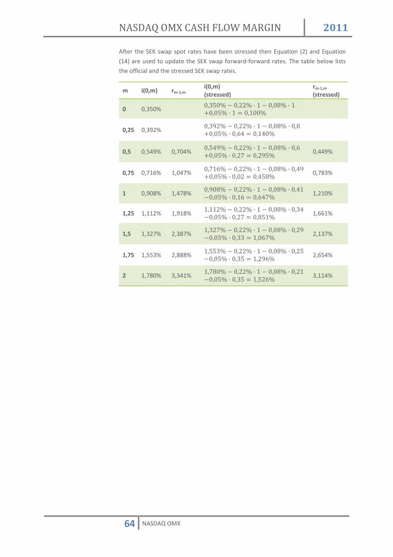
NASDAQ OMX CASH FLOW MARGIN 2011
64 NASDAQ OMX
After the SEK swap spot rates have been stressed then Equation (2) and Equation
(14) are used to update the SEK swap forward-forward rates. The table below lists
the official and the stressed SEK swap rates.
m i(0,m) rm-1,m i(0,m) (stressed)
rm-1,m
(stressed)
0 0,350% ��[2�] � ��33] , 4 � ���S] , 4 *���2] , 4 ��4��]
0,25 0,392% ��[T3] � ��33] , 4 � ���S] , ��S *���2] , ��j_ ��4_�]
0,5 0,549% 0,704% ��2_T] � ��33] , 4 � ���S] , ��j *���2] , ��3l ��3T2] 0,449%
0,75 0,716% 1,047% ��l4j] � ��33] , 4 � ���S] , ��_T *���2] , ���3 ��_2S] 0,783%
1 0,908% 1,478% ��T�S] � ��33] , 4 � ���S] , ��_4 ����2] , ��4j ��j_l] 1,210%
1,25 1,112% 1,918% 4�443] � ��33] , 4 � ���S] , ��[_ ����2] , ��3l ��S24] 1,661%
1,5 1,327% 2,387% 4�[3l] � ��33] , 4 � ���S] , ��3T ����2] , ��[[ 4��jl] 2,137%
1,75 1,553% 2,888% 4�22[] � ��33] , 4 � ���S] , ��32 ����2] , ��[2 4�3Tj] 2,654%
2 1,780% 3,341% 4�lS�] � ��33] , 4 � ���S] , ��34 ����2] , ��[2 4�23j] 3,114%

NASDAQ OMX CASH FLOW MARGIN 2011
65 NASDAQ OMX
NE T P R E S E N T V A L U E
The margin requirement is obtained by calculating the net present value of the cash
flows in all cash flow tables.
In this example all cash flows are in SEK and lay in the swap cash flow table. If the
net present value is calculated with the official SEK swap spot curve, then the
position’s market value is obtained. If, on the other hand, the net present value is
calculated with the stressed SEK swap spot curve, then the position’s margin
requirement is obtained.
Value date Time to maturity
SEK (floating) SEK (floating, stressed)
SEK (fixed)
2010-02-04 0,25 978
2010-05-04 0,5 4��������� , ��l�_], T�[j� 4�lj�
4��������� , ��__T], T�[j� 4�43[
2010-08-04 0,75 4��������� , 4��_l], T�[j� 3�j4S
4��������� , ��lS[], T�[j� 4�T2S
2010-11-04 1 4��������� , 4�_lS], T�[j� [�jT2
4��������� , 4�34�], T�[j� [��32 -17 730
2011-02-04 1,25 4��������� , 4�T4S], T�[j� _�lT2
4��������� , 4�jj4], T�[j� _�42[
2011-05-04 1,5 4��������� , 3�[SS], T�[j� 2�Tl�
4��������� , 3�4[l], T�[j� 2�[_[
2011-08-04 1,75 4��������� , 3�SST], T�[j� l�33[
4��������� , 3�j2_], T�[j� j�j[2
2011-11-04 2 4��������� , [�[_4], T�[j� S�[2[
4��������� , [�44_], T�[j� l�lS2 -17 730
NPV
TlS�4 * ��[T3]�W�U� * 4�lj��4 * ��2_T]�W�� *¸* S�[2[�4 * 4�lS�]�U
� 4l�l[��4 * 4�lS�]�U �44
NPV stressed
TlS�4 * ��4_�]�W�U� * 4�43[�4 * ��3T2]�W�� *¸* l�lS2�4 * 4�23j]�U
� 4l�l[��4 * 4�23j]�U �_�[2[
Market value = SEK -11.
Margin requirement = SEK -4 353.

NASDAQ OMX CASH FLOW MARGIN 2011
66 NASDAQ OMX
EXAMPLE 6 INT ER EST RA TE SW AP VER S US FRA
PO S I T I O N S
Consider a bought 2Y plain vanilla SEK fixed for floating interest rate swap that is
hedged with a strip of sold FRA contracts. These positions are traded on 2009-11-02,
but the margin calculation presented here is performed on 2009-11-04. In this
example it has, for simplicity, been assumed that all floating rate periods have 90
days and that all fixed rate periods have 360 days.
2Y I N T E R E S T R A T E S W A P
ts = 2009-11-04. te = 2011-11-04. Q = 1. N = 1 000 000. Side = 1. di,i+1 = 90. rfl = 0,391%. rf = 1,773%. df,i,i+1 = 360.
ST R I P O F F O R W A R D R A T E AG R E E M E N T S
FRA 1 2
tm = 2010-02-04. Q = 1. N = 1 000 000. Side = -1. d1,2 = 90. rc = 0,704%.
FRA 2 3
tm = 2010-05-04. Q = 1. N = 1 000 000. Side = -1. d2,3 = 90. rc = 1,047%.
FRA 3 4
tm = 2010-08-04. Q = 1. N = 1 000 000. Side = -1. d3,4 = 90. rc = 1,478%.

NASDAQ OMX CASH FLOW MARGIN 2011
67 NASDAQ OMX
FRA 4 5
tm = 2010-11-04. Q = 1. N = 1 000 000. Side = -1. d4,5 = 90. rc = 1,918%.
FRA 5 6
tm = 2011-02-04. Q = 1. N = 1 000 000. Side = -1. d5,6 = 90. rc = 2,388%.
FRA 6 7
tm = 2011-05-04. Q = 1. N = 1 000 000. Side = -1. d6,7 = 90. rc = 2,889%.
FRA 7 8
tm = 2011-08-04. Q = 1. N = 1 000 000. Side = -1. d7,8 = 90. rc = 3,341%.

NASDAQ OMX CASH FLOW MARGIN 2011
68 NASDAQ OMX
C A S H F L O W T A B L E S
2Y I N T E R E S T R A T E S W A P
Equation (13) is used to insert the floating cash flows into the FRA and swap cash
flow table. Equations (15) – (16) are used to insert the fixed cash flows into the FRA
and swap cash flow table. It should be noted that the value of the floating cash
flows will be updated when the swap spot curve changes.
ST R I P O F F O R W A R D R A T E AG R E E M E N T S
Equations (17) – (18) are used to insert the FRA contracts into the FRA and swap
cash flow tables. The profit and loss from a FRA contract is a floating cash flow, and
hence it will be updated when the swap spot curve changes.
FRA A N D S W A P C A S H F L O W T A B L E ( S W A P C U R V E )
Value date m SEK (floating) SEK (fixed)
2010-02-04 0,25 4�������� , ���l�_]� 7X�U� , T�[j��4 * 7X�U s T�[j�� 4��������� , ��[T4] , T�[j� TlS
2010-05-04 0,5
4�������� , �4��_l]� 7U��� , T�[j��4 * 7U�� s T�[j��
*4��������� , 7X�U , T�[j�
2010-08-04 0,75
4�������� , �4�_lS]� 7��k� , T�[j��4 * 7��k s T�[j��
*4��������� , 7U�� , T�[j�
2010-11-04 1
4�������� , �4�T4S]� 7k��� , T�[j��4 * 7k�� s T�[j��
*4��������� , 7��k , T�[j�
�4��������� , 4�ll[] , [j�[j� �4l�l[�
2011-02-04 1,25
4�������� , �3�[SS]� 7���� , T�[j��4 * 7��� s T�[j��
*4��������� , 7k�� , T�[j�
2011-05-04 1,5
4�������� , �3�SST]� 7��^� , T�[j��4 * 7��^ s T�[j��
*4��������� , 7��� , T�[j�
2011-08-04 1,75
4�������� , �[�[_4]� 7̂ �m� , T�[j��4 * 7̂ �m s T�[j��
*4��������� , 7��^ , T�[j�
2011-11-04 2 4��������� , 7̂ �m , T�[j� �4��������� , 4�ll[] , [j�[j� �4l�l[�

NASDAQ OMX CASH FLOW MARGIN 2011
69 NASDAQ OMX
C U R V E S T R E S S I N G
This position is exposed to a shift in the SEK swap spot curve. It is this curve that will
be stressed in the margin calculation.
R I S K P A R A M E T E R S
The tables below list the stress levels together with the first points on the principal
components for the SEK swap curve.
ST R E S S L E V E L S
Curve PC1 PC2 PC3 Swap 22 basis points 8 basis points 5 basis points
PR I N C I P A L C O M P O N E N T S
Time to maturity PC1 PC2 PC3 0 1 1 1 0,25 1 0,8 0,64 0,5 1 0,6 0,27 0,75 1 0,49 0,02 1 1 0,41 -0,16 1,25 1 0,34 -0,27 1,5 1 0,29 -0,33 1,75 1 0,25 -0,35 2 1 0,21 -0,35
OF F I C I A L C U R V E S
NOMX will, on each trading day, bootstrap official yield curves that will be used to
price all cleared instruments. It is the official yield curves that will be stressed in the
margin calculations. In this example it is assumed that the official SEK swap spot and
forward-forward curves look as in the figure below.
Figure: Official SEK swap curves from 2009-11-04.
0.000%
1.000%
2.000%
3.000%
4.000%
5.000%
6.000%
00.
5 11.
5 22.
5 33.
5 44.
5 55.
5 66.
5 77.
5 88.
5 99.
5 10
Official SEK spot Official SEK forward-forward

NASDAQ OMX CASH FLOW MARGIN 2011
70 NASDAQ OMX
The table below lists the official swap spot and forward-forward rates for the
maturities that are relevant to the cash flows in the swap cash flow table. Equation
(2) has been used to calculate the forward-forward rates,������� ����� from the
spot rates� ������. Equation (14) has then been used to convert the forward-forward rates into non-compounded forward-forward rates� 7ÃÄ�ÃÅ .
m i(0,m) f(0,m-1,m) rm-1,m 0 0,350%
0,25 0,392%
0,5 0,549% Æ�4 * ��2_T]�XmW��W�4 * ��[T3]� VW��WÇ
��WVW � 4 ��l�j]
[j�T� ��4 * ��l�j]� VW��W � 4� ��l�_]
0,75 0,716% Æ�4 * ��l4j]�U^W��W�4 * ��2_T]�XmW��WÇ
��WVW � 4� 4��24]
[j�T� ��4 * 4��24]� VW��W � 4� 4��_l]
1 0,908% Æ�4 * ��T�S]���W��W�4 * ��l4j]�U^W��WÇ
��WVW � 4 4�_Sj]
[j�T� ��4 * 4�_Sj]� VW��W � 4� 4�_lS]
1,25 1,112% Æ�4 * 4�443]�k�W��W�4 * ��T�S]���W��WÇ
��WVW � 4 4�T[3]
[j�T� ��4 * 4�T[3]� VW��W � 4� 4�T4S]
1,5 1,327% Æ�4 * 4�[3l]��kW��W�4 * 4�443]�k�W��WÇ
��WVW � 4 3�_�T]
[j�T� ��4 * 3�_�T]� VW��W � 4� 3�[SS]
1,75 1,553% Æ�4 * 4�22[]���W��W�4 * 4�[3l]��kW��WÇ
��WVW � 4 3�T3�]
[j�T� ��4 * 3�T3�]� VW��W � 4� 3�SST]
2 1,780% Æ�4 * 4�lS�]�^UW��W�4 * 4�22[]���W��WÇ
��WVW � 4 [�[S[]
[j�T� ��4 * [�[S[]� VW��W � 4� [�[_4]

NASDAQ OMX CASH FLOW MARGIN 2011
71 NASDAQ OMX
ST R E S S E D C U R V E S
The FRA contracts are traded at the official forward-forward rates. The worst
outcome for the sold FRA contracts is that the SEK swap forward-forward curve
increases and the worst outcome for the interest rate swap is that the SEK swap
spot curve drops. The FRA contracts will therefore generate a profit when the
interest rate swap generates a loss and vice versa. This combined position can
therefore be considered to be a hedged position.
Figure: Profit and loss for the sold FRA strip and the bought interest rate swap as the
SEK swap spot curve is stressed with and upward parallel shift of 22 basis points.
For this combined position it turns out that the Swap contract is slightly more
sensitive to an interest rate change compared to the FRA contracts. This implies that
the worst outcome is that the SEK swap spot curve decreases. This corresponds to
the scenario when the first two principal components are stressed downwards and
the third principal component is stressed upwards.
Figure: SEK swap spot curve will be stressed with its principal components.
-5,000.00
-4,000.00
-3,000.00
-2,000.00
-1,000.00
0.00
1,000.00
2,000.00
3,000.00
4,000.00
5,000.00
PnL FRA PnL IRS
-0.30%
-0.25%
-0.20%
-0.15%
-0.10%
-0.05%
0.00%
0.05%
0.10%
00.
5 11.
5 22.
5 33.
5 44.
5 55.
5 66.
5 77.
5 88.
5 99.
5 10
PC1 PC2 PC3 Combined stressing

NASDAQ OMX CASH FLOW MARGIN 2011
72 NASDAQ OMX
Figure: Official SEK swap curves and stressed SEK swap curve.
After the SEK swap spot rates have been stressed then Equation (2) and Equation
(14) are used to update the SEK swap forward-forward rates. The table below list
the official and the stressed SEK swap rates.
m i(0,m) rm-1,m i(0,m) (stressed)
rm-1,m
(stressed)
0 0,350% ��[2�] � ��33] , 4 � ���S] , 4 *���2] , 4 ��4��]
0,25 0,392% ��[T3] � ��33] , 4 � ���S] , ��S *���2] , ��j_ ��4_�]
0,5 0,549% 0,704% ��2_T] � ��33] , 4 � ���S] , ��j *���2] , ��3l ��3T2] 0,449%
0,75 0,716% 1,047% ��l4j] � ��33] , 4 � ���S] , ��_T *���2] , ���3 ��_2S] 0,783%
1 0,908% 1,478% ��T�S] � ��33] , 4 � ���S] , ��_4 ����2] , ��4j ��j_l] 1,210%
1,25 1,112% 1,918% 4�443] � ��33] , 4 � ���S] , ��[_ ����2] , ��3l ��S24] 1,661%
1,5 1,327% 2,387% 4�[3l] � ��33] , 4 � ���S] , ��3T ����2] , ��[[ 4��jl] 2,137%
1,75 1,553% 2,888% 4�22[] � ��33] , 4 � ���S] , ��32 ����2] , ��[2 4�3Tj] 2,654%
2 1,780% 3,341% 4�lS�] � ��33] , 4 � ���S] , ��34 ����2] , ��[2 4�23j] 3,114%
0.000%
1.000%
2.000%
3.000%
4.000%
5.000%
6.000%
00.
5 11.
5 22.
5 33.
5 44.
5 55.
5 66.
5 77.
5 88.
5 99.
5 10
Official SEK spot Official SEK forward-forward
Stressed SEK spot Stressed SEK forward-forward

NASDAQ OMX CASH FLOW MARGIN 2011
73 NASDAQ OMX
NE T P R E S E N T V A L U E
The margin requirement is obtained by calculating the net present value of the cash
flows in the cash flow table. In this example all cash flows are in SEK and are
exposed to the swap curve. If the net present value is calculated with the official SEK
swap spot curve, then the position’s market value is obtained. If, on the other hand,
the net present value is calculated with the stressed SEK swap spot curve, then the
position’s margin requirement is obtained.
m SEK (floating) SEK (floating, stressed) SEK
(fixed)
0,25
4��������� , ���l�_]� ��l�_]� , T�[j��4 * ��l�_] s T�[j��
�
4��������� , ���l�_]� ��__T]� , T�[j��4 * ��__T] s T�[j��
j[l
978
0,5
4��������� , �4��_l]� 4��_l]� , T�[j��4 * 4��_l] s T�[j��
*4��������� , ��l�_] , T�[j� 4�lj�
4��������� , �4��_l]� ��lS[]� , T�[j��4 * ��lS[] s T�[j��
*4��������� , ��__T] , T�[j� 4�lS3
0,75
4��������� , �4�_lS]� 4�_lS]� , T�[j��4 * 4�_lS] s T�[j��
*4��������� , 4��_l] , T�[j� 3�j4S
4��������� , �4�_lS]� 4�34�]� , T�[j��4 * 4�34�] s T�[j��
*4��������� , ��lS[] , T�[j� 3�j3j
1
4��������� , �4�T4S]� 4�T4S]� , T�[j��4 * 4�T4S] s T�[j��
*4��������� , 4�_lS] , T�[j� [�jT2
4��������� , �4�T4S]� 4�jj4]� , T�[j��4 * 4�jj4] s T�[j��
*4��������� , 4�34�] , T�[j� [�jj2
-17 730
1,25
4��������� , �3�[SS]� 3�[SS]� , T�[j��4 * 3�[SS] s T�[j��
*4��������� , 4�T4S] , T�[j� _�lT2
4��������� , �3�[SS]� 3�4[l]� , T�[j��4 * 3�4[l] s T�[j��
*4��������� , 4�jj4] , T�[j� _�lll
1,5
4��������� , �3�SST]� 3�SST]� , T�[j��4 * 3�SST] s T�[j��
*4��������� , 3�[SS] , T�[j� 2�Tl�
4��������� , �3�SST]� 3�j2_]� , T�[j��4 * 3�j2_] s T�[j��
*4��������� , 3�4[l] , T�[j� 2�T3j
1,75
4��������� , �[�[_4]� [�[_4]� , T�[j��4 * [�[_4] s T�[j��
*4��������� , 3�SST] , T�[j� l�33[
4��������� , �[�[_4]� [�44_]� , T�[j��4 * [�44_] s T�[j��
*4��������� , 3�j2_] , T�[j� l�4TT
2 4��������� , [�[_4] , T�[j� S�[2[ 4��������� , [�44_] , T�[j� l�lS2 -17 730
NPV � ��4 * ��[T3]�W�U� * TlS�4 * ��[T3]�W�U� *¸* S�[2[�4 * 4�lS�]�U
� 4l�l[��4 * 4�lS�]�U �44
NPV stressed
j[l�4 * ��4_�]�W�U� * TlS�4 * ��4_�]�W�U� *¸* llS2�4 * 4�23j]�U
� 4l�l[��4 * 4�23j]�U �42
Market value = SEK -11.
Margin requirement = SEK -15.

NASDAQ OMX CASH FLOW MARGIN 2011
74 NASDAQ OMX
It should be noted that this margin requirement is less than one percent of the FRA
contracts and the interest rate swaps combined naked margins.

NASDAQ OMX CASH FLOW MARGIN 2011
75 NASDAQ OMX
EXAMPLE 7 FRA PO RT FO LIO V ER SU S RIBA POR TFO LIO
PO S I T I O N S
Consider a bought 1Y strip of RIBA futures that is partly hedged with a 1Y strip of
sold FRA contracts. These positions are traded on 2011-08-01, but the margin
calculation presented here is performed on 2011-09-09. This means that for the
FRAs, it is the last settlement price, from 2011-08-31, that will determine their
current market value. The daily settled RIBA futures have a market value of zero
after each end of day. Here we use the RIBA fixing prices from 2011-09-09 as a
departing point when calculating the possible shifts in market value (i.e. the margin
requirement). In this example it has, for simplicity, been assumed that all floating
rate periods have 90 days and that all fixed rate periods have 360 days. Please note
that the expiration month codes differ between a RIBA future and a FRA on the
same underlying time period.
ST R I P O F R I B A F U T U R E S
RIBA11Z
tm = 2011-12-21.
Q = 2. N = 1 000 000. Side = 1. d1,2 = 90. rc = 1,93%.
RIBA12H
tm = 2012-03-21. Q = 2. N = 1 000 000. Side = 1. d2,3 = 90. rc = 1,635%.
RIBA12M
tm = 2012-06-20. Q = 2. N = 1 000 000. Side = 1. d3,4 = 90. rc = 1,35%.
RIBA12U
tm = 2012-09-19. Q = 2. N = 1 000 000. Side = 1. d3,4 = 90.

NASDAQ OMX CASH FLOW MARGIN 2011
76 NASDAQ OMX
rc = 1,19%.
ST R I P O F F O R W A R D R A T E AG R E E M E N T S
FRA11U
tm = 2011-09-21. Q = 1. N = 1 000 000. Side = -1. d1,2 = 90. rc = 2,603%.
FRA11X
tm = 2011-12-21. Q = 1. N = 1 000 000. Side = -1. d2,3 = 90. rc = 2,413%.
FRA12O
tm = 2012-03-21. Q = 1. N = 1 000 000. Side = -1. d3,4 = 90. rc = 2,24%.
FRA12R
tm = 2012-06-20. Q = 1. N = 1 000 000. Side = -1. d4,5 = 90. rc = 2,133%.

NASDAQ OMX CASH FLOW MARGIN 2011
77 NASDAQ OMX
C A S H F L O W T A B L E S
ST R I P O F RIBA F U T U R E S
Equations (22) – (24) are used to insert the RIBA futures contracts into the RIBA cash
flow tables. The profit and loss from a RIBA futures contract is a floating cash flow,
and hence it will be updated when the RIBA curve changes. Note that no
discounting of cash flows will take place, the stressed NPV of a RIBA future is
determined solely by the forecasted floating cash flow.
RIBA C A S H F L O W T A B L E ( RIBA C U R V E )
Value date
m SEK (floating)
2011-12-21 0,2822 3�������� , ��4�T[]* 7UWXXWVUX�UWXXXUUX� , T�È[j�
2012-03-21 0,5315 3�������� , ��4�j[2]* 7UWXXXUUX=UWXUW�UX� , T�È[j�
2012-06-20 0,7808 3�������� , ��4�[2]* 7UWXUW�UX�UWXUW�UW� , T�È[j�
2012-09-19 1,0301 3�������� , ��4�4T]* 7UWXUW�UW�UWXUWVXV� , T�È[j�
ST R I P O F F O R W A R D R A T E AG R E E M E N T S
Equations (17) – (18) are used to insert the FRA contracts into the FRA and swap
cash flow tables. The profit and loss from a FRA contract is a floating cash flow, and
hence it will be updated when the swap spot curve changes.
FRA A N D S W A P C A S H F L O W T A B L E ( S W A P C U R V E )
Value date m SEK (floating) 2011-09-21 0,0329 4�������� , �3�j�[]� 7UWXXWVUX�UWXXXUUX� , T�[j��4 * 7UWXXWVUX�UWXXXUUX s T�[j��
2011-12-21 0,2822 4�������� , �3�_4[]� 7UWXXXUUX�UWXUW�UX� , T�[j��4 * 7UWXXXUUX�UWXUW�UX s T�[j��
2012-03-21 0,5315 4�������� , �3�3_]� 7UWXUW�UX�UWXUW�UW� , T�[j��4 * 7UWXUW�UX�UWXUW�UW s T�[j��
2012-06-20 0,7808 4�������� , �3�4[[]� 7UWXUW�UW�UWXUWVXV� , T�[j��4 * 7UWXUW�UW�UWXUWVXV s T�[j��
C U R V E S T R E S S I N G

NASDAQ OMX CASH FLOW MARGIN 2011
78 NASDAQ OMX
This position is exposed to shifts in the SEK swap spot curve and in the RIBA spot
curve. These curves will be stressed in the margin calculation, and their inter curve
correlation will influence the way in which the total portfolio is margined.
R I S K P A R A M E T E R S
The tables below list the stress levels together with the first eight quarters on the
principal components for the SEK swap curve. When estimating the principal
components’ levels for other points on the time axis a linear interpolation is used.
ST R E S S L E V E L S
Curve PC1 PC2 PC3 Swap 22 basis points 8 basis points 5 basis points RIBA 22 basis points 8 basis points 5 basis points
PR I N C I P A L C O M P O N E N T S
Time to maturity PC1 PC2 PC3
0 1 1 1 0,25 1 0,8 0,64 0,5 1 0,6 0,27 0,75 1 0,49 0,02 1 1 0,41 -0,16 1,25 1 0,34 -0,27 1,5 1 0,29 -0,33 1,75 1 0,25 -0,35 2 1 0,21 -0,35 2,25 1 0,18 -0,32
C O R R E L A T I O N
In this example the scanning range in each principal component is divided into 5
steps, yielding a total of 5 * 5 * 5 = 125 different scenarios for which the shift in
market value is calculated. We use a correlation cube of size 3 * 3 * 3 between the
two curves to account for their co-variation.
OF F I C I A L C U R V E S
NOMX will, on each trading day, bootstrap official yield curves that will be used to
price all cleared instruments. It is the official yield curves that will be stressed in the
margin calculations. In this example it is assumed that the official SEK swap spot and
RIBA spot curves look as in the figure below.

NASDAQ OMX CASH FLOW MARGIN
79 NASDAQ OMX
Figure: Official SEK swap
ST R E S S E D C U R V E S
The long position (pay contracted rate) in the RIBA strip is exposed to a downward
shift of the RIBA curve. The short position (receive contracted rate) in the FRA strip
is exposed to an upward shift in the SEK Swap curve. If no correlation benefits were
offered between the two curves they would be stressed in opposite directions in the
margin calculation. The effect is illustrated below.
Figure: Curve stress that would resul
As mentioned before, however, in this case there is a modeled correlation between
the two curves. This would be a result of NOMX RM observing correlation between
the two curves in historical time series. The correlation
the total scenario cubes is of size 5*5*5, that means that we will margin our
positions across the 3*3*3 sub
this case it results in the RIBA curve being stressed as if it w
ASDAQ OMX CASH FLOW MARGIN
NASDAQ OMX
Figure: Official SEK swap & RIBA curves from 2011-09-09.
T R E S S E D C U R V E S
The long position (pay contracted rate) in the RIBA strip is exposed to a downward
shift of the RIBA curve. The short position (receive contracted rate) in the FRA strip
exposed to an upward shift in the SEK Swap curve. If no correlation benefits were
offered between the two curves they would be stressed in opposite directions in the
margin calculation. The effect is illustrated below.
Curve stress that would result if no correlation was configured
As mentioned before, however, in this case there is a modeled correlation between
the two curves. This would be a result of NOMX RM observing correlation between
the two curves in historical time series. The correlation cube is set to 3*3*3, and as
the total scenario cubes is of size 5*5*5, that means that we will margin our
positions across the 3*3*3 sub-space of scenarios that yields the lowest margin. In
this case it results in the RIBA curve being stressed as if it was a naked position. This
2011
The long position (pay contracted rate) in the RIBA strip is exposed to a downward
shift of the RIBA curve. The short position (receive contracted rate) in the FRA strip
exposed to an upward shift in the SEK Swap curve. If no correlation benefits were
offered between the two curves they would be stressed in opposite directions in the
t if no correlation was configured
As mentioned before, however, in this case there is a modeled correlation between
the two curves. This would be a result of NOMX RM observing correlation between
cube is set to 3*3*3, and as
the total scenario cubes is of size 5*5*5, that means that we will margin our
space of scenarios that yields the lowest margin. In
as a naked position. This
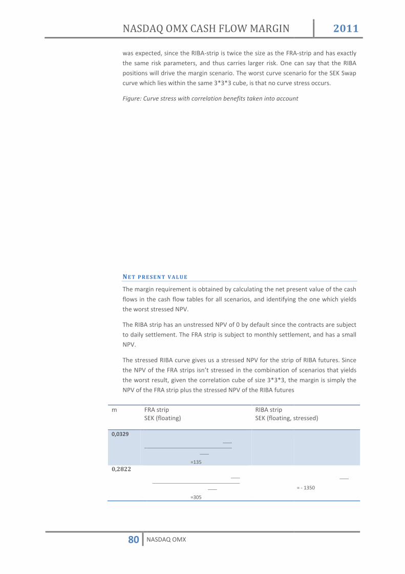
NASDAQ OMX CASH FLOW MARGIN
80 NASDAQ OMX
was expected, since the RIBA
the same risk parameters, and thus carries larger risk. One can say that the RIBA
positions
curve which lies within the same 3*3*3 cube, is that no curve stress occurs.
Figure: Curve stress with correlation benefits taken into account
NE T P R E S E N T V A L U E
The margin requirement is obtained by calculating the net present valu
flows in the cash flow tables for all scenarios, and identifying the one which yields
the worst stressed NPV.
The RIBA strip has an unstressed NPV of 0 by default since the contracts are subject
to daily settlement. The FRA strip is subject t
NPV.
The stressed RIBA curve gives us a stressed NPV for the strip of RIBA futures. Since
the NPV of the FRA strips isn’t stressed in the combination of scenarios that yields
the worst result, given the correlation cub
NPV of the FRA strip plus the stressed NPV of the RIBA futures
m FRA stripSEK (floating)
0,0329
0,2822
ASDAQ OMX CASH FLOW MARGIN
NASDAQ OMX
was expected, since the RIBA-strip is twice the size as the FRA
the same risk parameters, and thus carries larger risk. One can say that the RIBA
positions will drive the margin scenario. The worst curve scen
curve which lies within the same 3*3*3 cube, is that no curve stress occurs.
Curve stress with correlation benefits taken into account
E T P R E S E N T V A L U E
The margin requirement is obtained by calculating the net present valu
flows in the cash flow tables for all scenarios, and identifying the one which yields
the worst stressed NPV.
The RIBA strip has an unstressed NPV of 0 by default since the contracts are subject
to daily settlement. The FRA strip is subject to monthly settlement, and has a small
The stressed RIBA curve gives us a stressed NPV for the strip of RIBA futures. Since
the NPV of the FRA strips isn’t stressed in the combination of scenarios that yields
the worst result, given the correlation cube of size 3*3*3, the margin is simply the
NPV of the FRA strip plus the stressed NPV of the RIBA futures
FRA strip SEK (floating)
RIBA strip SEK (floating, stressed)
=135
=305
2011
strip is twice the size as the FRA-strip and has exactly
the same risk parameters, and thus carries larger risk. One can say that the RIBA
will drive the margin scenario. The worst curve scenario for the SEK Swap
curve which lies within the same 3*3*3 cube, is that no curve stress occurs.
Curve stress with correlation benefits taken into account
The margin requirement is obtained by calculating the net present value of the cash
flows in the cash flow tables for all scenarios, and identifying the one which yields
The RIBA strip has an unstressed NPV of 0 by default since the contracts are subject
o monthly settlement, and has a small
The stressed RIBA curve gives us a stressed NPV for the strip of RIBA futures. Since
the NPV of the FRA strips isn’t stressed in the combination of scenarios that yields
e of size 3*3*3, the margin is simply the
NPV of the FRA strip plus the stressed NPV of the RIBA futures
SEK (floating, stressed)
= - 1350

NASDAQ OMX CASH FLOW MARGIN 2011
81 NASDAQ OMX
Market value = SEK 1575
Margin requirement = SEK -3800.
0,5315 4�������� , �3�3_]� 4�T[]� , T�[j��4 * 4�T[] s T�[j��
=523
3�������� , ��4�j[2]* 4�[l]� , T�[j�
= - 1325
0,7808 4�������� , �3�4[[]� 4�ljS]� , T�[j��4 * 4�ljS] s T�[j��
=633
3�������� , ��4�[2]* 4��S]� , T�[j�
= -1350
1,0301 3�������� , ��4�4T]* ��T3]� , T�[j�
= -1350
4[2�� * /� /¢]����1/¢ �* � [�2�� * /� C£]���/¤// *� 23[�� * /� £¥]���O1�O*� j[[�� * /� 1�]���¥¤�¤�����
NPV RIBA (unstressed) = 0 NPV FRA (unstressed) = �
= 1575 NPV RIBA (stressed) = -1350 - 1325 – 1350 - 1350 = -5375

NASDAQ OMX CASH FLOW MARGIN 2011
82 NASDAQ OMX
EXAMPLE 8 FUT UR E CONT RA CT S WI TH D AI LY S ETT LEMENT
PO S I T I O N S
Consider the below portfolio of 100 bought 3MSTIBZ1 (Futures contract on the 3
month STIBOR). The future has daily settlement so the market value end of day will
be equal to zero. The position is traded on 2011-09-02, but the margin calculation
presented here is performed on 2011-09-22.
3M S T I B Z1
tm = 2011-12-21. Q = 100. N = 1 000 000. Side = 1. d1,2 = 90. Pc = 97,559 rc = 2,441%
C A S H F L O W S
Equations (25) and (26) is used to insert the STIBOR futures contracts into the SEK
Swap cash flow tables. The profit and loss from a STIBOR future contract is a floatin
cash flow, and hence it will be updated when the SEK Swap curve changes. Note
that no discounting of cash flows will take place, the stressed NPV of the STIBOR
future is determined solely by the forecasted floating cash flows.
-Mp�ÉÊËÌÍÎX�$��� �� $0� � , ��� , ��������� , �3�__4] ��$/����//��/��/�1/�� , T�1C�
The floating cash flow will be decided by the forward-forward rate from the curve.
C U R V E S T R E S S I N G
This position is exposed to a shift in the SEK swap spot curve. It is this curve that will
be stressed in the margin calculation.
R I S K P A R A M E T E R S
The tables below list the stress levels together with the first points on the principal
components for the SEK swap curve.
ST R E S S L E V E L S
Curve PC1 PC2 PC3 Swap 22 basis points 8 basis points 5 basis points
PR I N C I P A L C O M P O N E N T S
Time to maturity PC1 PC2 PC3 0 1 1 1 0,25 1 0,8 0,64

NASDAQ OMX CASH FLOW MARGIN 2011
83 NASDAQ OMX
0,5 1 0,6 0,27 0,75 1 0,49 0,02 1 1 0,41 -0,16 1,25 1 0,34 -0,27 1,5 1 0,29 -0,33 1,75 1 0,25 -0,35 2 1 0,21 -0,35
The shape of the SEK swap curve’s principal components is shown in the figure
below.
Figure: Shape of the SEK swap curve’s principal components.
OF F I C I A L C U R V E S
NOMX will, on each trading day, bootstrap official yield curves that will be used to
price all cleared instruments. It is the official yield curves that will be stressed in the
margin calculations. In this example it is assumed that the official SEK swap spot
curve look as in the figure below.
Figure: Swap curve
-0.6
-0.4
-0.2
0
0.2
0.4
0.6
0.8
1
1.2
00.
5 11.
5 22.
5 33.
5 44.
5 55.
5 66.
5 77.
5 88.
5 99.
5 10
PC1 PC2 PC3
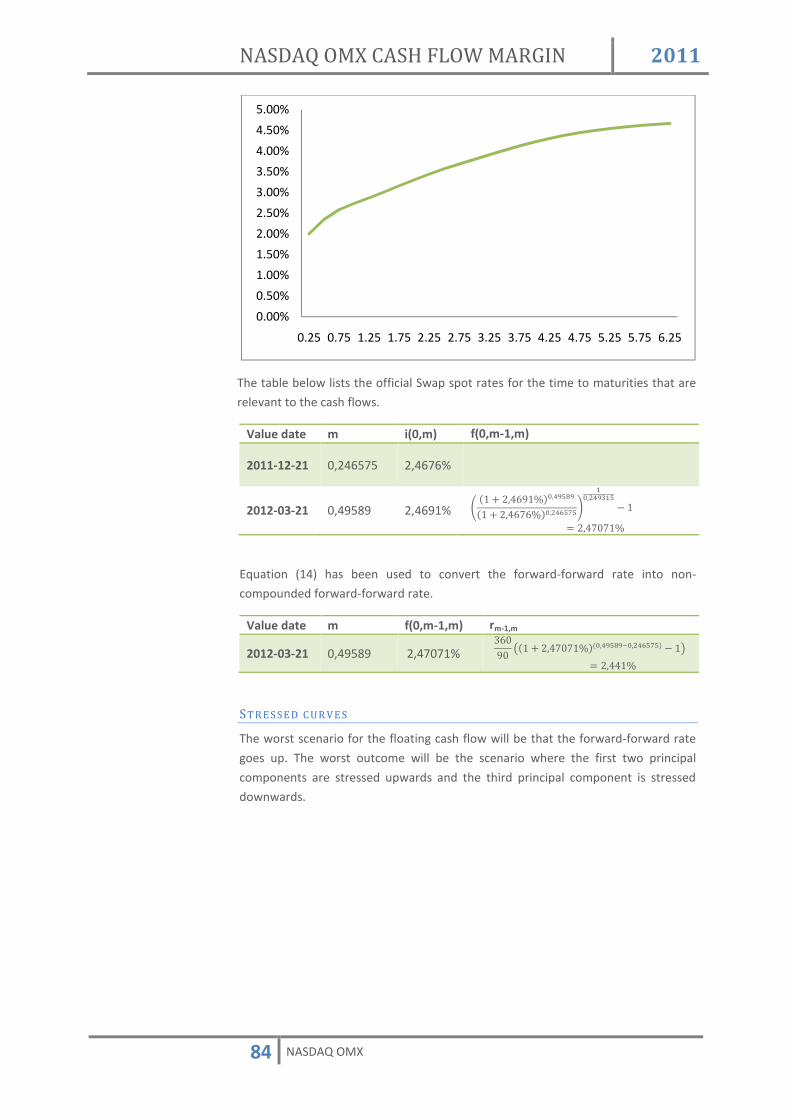
NASDAQ OMX CASH FLOW MARGIN 2011
84 NASDAQ OMX
The table below lists the official Swap spot rates for the time to maturities that are
relevant to the cash flows.
Value date m i(0,m) f(0,m-1,m)
2011-12-21 0,246575 2,4676%
2012-03-21 0,49589 2,4691% ± �4 * 3�_jT4]�W�kV�mV�4 * 3�_jlj]�W�Uk��^�²XW�UkV�X� � 4
3�_l�l4]
Equation (14) has been used to convert the forward-forward rate into non-
compounded forward-forward rate.
Value date m f(0,m-1,m) rm-1,m
2012-03-21 0,49589 2,47071% [j�T� ��4 * 3�_l�l4]��W�kV�mVW�Uk��^�� � 4� 3�__4]
ST R E S S E D C U R V E S
The worst scenario for the floating cash flow will be that the forward-forward rate
goes up. The worst outcome will be the scenario where the first two principal
components are stressed upwards and the third principal component is stressed
downwards.
0.00%
0.50%
1.00%
1.50%
2.00%
2.50%
3.00%
3.50%
4.00%
4.50%
5.00%
0.25 0.75 1.25 1.75 2.25 2.75 3.25 3.75 4.25 4.75 5.25 5.75 6.25

NASDAQ OMX CASH FLOW MARGIN 2011
85 NASDAQ OMX
Figure: The worst scenario is when the Swap curve is stressed upward.
Figure: Official Swap curve and stressed Swap curve
NOMX defines the principal components in a predefined number of nodes. The
distance between each node is in this example 0,25 years. A linear interpolation will
be used in order to determine the stress levels for the different maturities. This can
be seen in the table below.
Time to maturity
PC1 PC2 PC3
0 1 1 1
0,246575 1 4 * ��S � 4��32 � �, ���3_j2l2 � �� ��S�3l_
4 * ��j_ � 4��32 � � , ���3_j2l2 � �� ��j__T[
0,25 1 0,8 0,64
0,49589
1 ��S * ��j � ��S��2 � ��32, ���_T2ST� ��32� ��j�[3T
��j_ * ��3l � ��j_��2 � ��32 , ���_T2ST� ��32� ��3lj�S
0,5 1 0,6 0,27
-0.001
-0.0005
0
0.0005
0.001
0.0015
0.002
0.0025
0.003
0.25 0.5 0.75 1 1.25 1.5 1.75 2 2.25 2.5
PC1
PC2
PC3
Combined
0.00%
1.00%
2.00%
3.00%
4.00%
5.00%
6.00%
0.25 0.75 1.25 1.75 2.25 2.75 3.25 3.75 4.25 4.75 5.25 5.75 6.25
Spot Stressed

NASDAQ OMX CASH FLOW MARGIN 2011
86 NASDAQ OMX
The table below shows the stressed Swap spot rates when the three principal
components are stressed.
Time to maturity Spot rate Stressed spot rate 0,246575 3�_jlj] 3�_jlj] * ��33] , 4 * ���S] , �S�3l_ � ���2], ��j__T[ 3�l3�]
0,49589 3�_jT4] 3�_jT4] * ��33] , 4 * ���S] , ��j�[3T � ���2], ��3lj�S 3�l3_]
The table below shows the stressed Swap forward-forward rates when the three
principal components are stressed.
m i(0,m) f(0,m-1,m) rm-1,m
0,246575 3�l3�]
0,49589 3�l3_] 3�l3S] 3�jT[]
Equation (26) is used to decide the stressed floating cash flow.
-Mp�ÉÊËÌÍÎX�$��� �� $0� � , ��� , ��������� , �3�__4] � �3�jT[]� , VW1C� = �j[����
Margin requirement = SEK -63 000.

NASDAQ OMX CASH FLOW MARGIN 2011
87 NASDAQ OMX
EXAMPLE 9 BOND FO RW AR D (NO N SYN TH ETI C)
PO S I T I O N S
Consider the below portfolio of 100 bought NBHYP2 (2-year Nordbanken Hypotek
Bond) contracts.
t = 2011-02-15 n = 3 N = SEK 1 000 000 C = 4,25. Q = 100 r = 3,50% rt = 3,55% d 93 de = 2011-03-10 dsett = 2011-03-16
Ci =
Payment 42 500 42 500 1 042 500
Date 2011-06-19 2012-06-19 2013-06-19
C A S H F L O W T A B L E
Equation (27) is used to calculate the trade price. It is 93 days between 2011-03-16
and 2011-06-19 in a 30E convention.
;º�» �[�2�]� 4������� , �_�32][�2�] , ��4 * [�2�]�� � 4� * 4�
��4 * [�2�]�� V���W �X�� 4��_l�[TS
This results in the following cash flow table.
Value date SEK
2011-03-16 -100 · 1 047 398 = -104 739 800
2011-06-19 100 · 42 500 = 4 250 000
2012-06-19 100 · 42 500 = 4 250 000
2013-06-19 100 · (42 500 + 1000 000) = 104 250 000

NASDAQ OMX CASH FLOW MARGIN 2011
88 NASDAQ OMX
C U R V E S T R E S S I N G
This position is exposed to a shift in the SEK NBHYP spot curve and it is this curve
that will be stressed in the margin calculation.
R I S K P A R A M E T E R S
The shape of the SEK NBHYP curve’s principal components is shown in the figure
below.
Figure: Shape of the SEK NBHYP curve’s principal components.
The tables below list the stress levels together with the first points of the principal
components for the SEK NBHYP curve.
ST R E S S L E V E L S
Curve PC1 PC2 PC3 NBHYP 25 basis points 15 basis points 10 basis points
PR I N C I P A L C O M P O N E N T S
Time to maturity PC1 PC2 PC3 0 1 1 1 0,25 1 0,8 0,64 0,5 1 0,6 0,27 0,75 1 0,49 0,02 1 1 0,41 -0,16 1,25 1 0,34 -0,27 1,5 1 0,29 -0,33 1,75 1 0,25 -0,35 2 1 0,21 -0,35 2,25 1 0,18 -0,32 2,5 1 0,15 -0,29
-0.6
-0.4
-0.2
0
0.2
0.4
0.6
0.8
1
1.20
0.5 1
1.5 2
2.5 3
3.5 4
4.5 5
5.5 6
6.5 7
7.5 8
8.5 9
9.5 10
PC1 PC2 PC3

NASDAQ OMX CASH FLOW MARGIN 2011
89 NASDAQ OMX
OF F I C I A L C U R V E S
NOMX will, on each trading day, bootstrap official yield curves that will be used to
price all cleared instruments. It is the official yield curves that will be stressed in the
margin calculations. The underlying bond is issued by Nordbanken Hypotek which
means that it will be Nordbanken Hypotek´s official yield curve (NBHYP) that will be
used in the margin calculations. In this example it is assumed that the official NBHYP
curve looks as in the figure below.
Figure: NBHYP curve
The table below lists the official NBHYP spot rates for the time to maturities that are
relevant to the cash flows.
Time to maturity Spot rate 0,07945 4�2�4]
0,34247 3��[T]
1,34247 3�T3_]
2,34247 [�_T[]
ST R E S S E D C U R V E S
The first cash flow is a negative one and thus the worst scenario for that cash flow
will be that all short NBHYP spot rates goes down. However, the position’s cash
flows that are most distance are the ones that are derived from the underlying
bond. These are all positive cash flows and hence these positions are mainly
exposed to an upward shift in the NBHYP curve. If one considers all cash flows, the
worst outcome will be the scenario where the first two principal components are
stressed upwards and the third principal component is stressed downwards.
0.00%0.50%1.00%1.50%2.00%2.50%3.00%3.50%4.00%4.50%5.00%
0.25 0.75 1.25 1.75 2.25 2.75 3.25 3.75 4.25 4.75 5.25 5.75 6.25
NBHYP

NASDAQ OMX CASH FLOW MARGIN 2011
90 NASDAQ OMX
Figure: The worst scenario is when the NBHYP curve is stressed upward.
Figure: Official NBHYP curve and stressed NBHYP curve
NOMX defines the principal components in a predefined number of nodes. The
distance between each node is in this example 0,25 years. A linear interpolation will
be used in order to determine the stress levels for the different maturities. This can
be seen in the table below.
Time to maturity
PC1 PC2 PC3
0 1 1 1
0,07945 1 4 * ��S � 4��32 � � , ����lT_2 � �� ��T[j__
4 * ��j_ � 4��32 � � , ����lT_2 � �� ��SS22T 0,25 1 0,8 0,64
0,33973
1 ��S * ��j � ��S��2 � ��32 , ���[[Tl[� ��32� ��l3S33
��j_ * ��3l � ��j_��2 � ��32 , ���[[Tl[� ��32� ��2�l3�
0,5 1 0,6 0,27
-0.15%
-0.10%
-0.05%
0.00%
0.05%
0.10%
0.15%
0.20%
0.25%
0.30%
0.35%
0 0.25 0.5 0.75 1 1.25 1.5 1.75 2 2.25 2.5
PC1 PC2 PC3 Combined
0.00%
1.00%
2.00%
3.00%
4.00%
5.00%
6.00%
0.25 0.75 1.25 1.75 2.25 2.75 3.25 3.75 4.25 4.75 5.25 5.75 6.25
Spot Stressed

NASDAQ OMX CASH FLOW MARGIN 2011
91 NASDAQ OMX
0,75 1 0,49 0,02
1 1 0,41 -0,16 1,25 1 0,34 -0,27
1,34247 1 ��[_ * ��3T � ��[_4�2 � 4�32 , �4�[_3_l� 4�32� ��[3424
���3l * ���[[ * ��3l4�2 � 4�32 , �4�[_3_l� 4�32� ���3T34T 1,5 1 0,29 -0,33
1,75 1 0,25 -0,35
2 1 0,21 -0,35
2,25 1 0,18 -0,32
2,34247 ��4S * ��42 � ��4S3�2 � 3�32 , �3�[_3_l� 3�32� ��4jST�
���[3 * ���3T * ��[33�2 � 3�32 , �3�[_3_l� 3�32� ���[�ST� 2,5 1 0,15 -0,29
The table below shows the stressed NBHYP spot rates when the three principal
components are stressed.
Time to maturity Spot rate Stressed spot rate 0,07945 4�2�4] 4�2�4] * ��32] , 4 * ��42] , ��T[j__ � ��4�], ��SS22T 4�S�[]
0,33973 3��[T] 3��[T] * ��32] , 4 * ��42] , ��l3S33 � ��4�], ��2�l3� 3�[_l]
1,34247 3�T3_] 3�T3_] * ��32] , 4 * ��42] , ��[3424 * ��4�], ��3T34T [�324]
2,34247 [�_T[] [�_T[] * ��32] , 4 * ��42] , ��4jST� * ��4�], ��[�ST� [�lTT]
NE T P R E S E N T V A L U E
The margin requirement is obtained by calculating the net present value of the cash
flows in the cash flow table.
In this example all cash flows are in SEK and are exposed to the NBHYP curve. It
should be noted that the NPV is calculated from a yield curve built up by bonds from
the issuer. The bond forward itself is not a calibration instrument and thus the
unstressed NPV will slightly deviate from the market value. However, when NOMX
presents the market value in e.g. margin reports the instrument will get its market
value from the margin price in the Price Server i.e. the market value will be
calculated from equation (19) and based on the difference between the traded price
(r) and today’s fixed price (rt). If, on the other hand, the net present value is
calculated with the stressed SEK NBHYP curve, then the bond forward position’s
margin requirement is obtained.

NASDAQ OMX CASH FLOW MARGIN 2011
92 NASDAQ OMX
Value date Time to maturity SEK 2011-03-16 0,07945 -104 739 800
2011-06-19 0,33973 4 250 000
2012-06-19 1,34247 4 250 000
2013-06-19 2,34247 104 250 000
Market value 4�� s N�ÏÐÑ��[�22]� ���ÏÐÑ��[�2�]�P �4�S�3���
NPV stressed �4�_�l[T�S���4 * 4�S�[]�W�W^Vk� *¸* 4�_�32������4 * [�lTT]�U��kUk^ �ll3�2[[
Market value = SEK -108 200
Margin requirement = SEK -772 533

NASDAQ OMX CASH FLOW MARGIN 2011
93 NASDAQ OMX
EXAMPLE 10 BOND FO RW AR D (SYN T H ETI C) Consider the below portfolio of 100 sold R2RR (government bond) contracts. The
forward contract is traded on the forward yield of the deliverable bond and thus the
bond forward will be valued by using the forward yield to maturity of the
deliverable bond as implied by the yield curve. The P/L is however calculated using
the characteristics of the synthetic bond. Using CFM to calculate margin for these
contracts therefore requires some additional steps compared to the usual cash flow
discounting used for most other interest rate derivatives. In short, the cash flows of
the synthetic bond forward will be forward valued, not by using the yield curve, but
by using the forward yield to maturity of the deliverable bond as implied by the
yield curve. The deliverable bond for R2RR is RGKB1041 with maturity 2014-05-05
and a coupon rate of 6,75%.
t = 2011-03-02 n = 3 N = SEK 1 000 000 C = 6,75. Q = -100 r = 2,99% rt = 2,99% d = 320 de = 2011-06-09 dsett = 2011-06-15 dc = 2012-05-05 Ci =
Payment 67 500 67 500 1 067 500
Date 2012-05-05 2013-05-05 2014-05-05
Equation (27) is used to calculate the trade price. It is 320 days between 2011-06-15
and 2012-05-05 in a 30E convention.
;º�» �3�TT]� 4������� , �j�l2]3�TT] , ��4 * 3�TT]�� � 4� * 4�
��4 * 3�TT]���UW��W �X�� 4�44����_
This would result in the following cash flow table.
Value date SEK
2011-06-15 100 · 1 110 004 = 111 000 400
2012-05-05 -100 · 67 500 = -6 750 000
2013-05-05 -100 · 67 500 = -6 750 000
2014-05-05 -100 · (67 500 + 1000 000) = -106 750 000
The forward-forward rate �������i� will be derived from the treasury curve. The
forward-forward rates and the above cash flows are inserted into Equation (20) to
calculate the forward price quoted in yield of the deliverable bond. Equation (19)
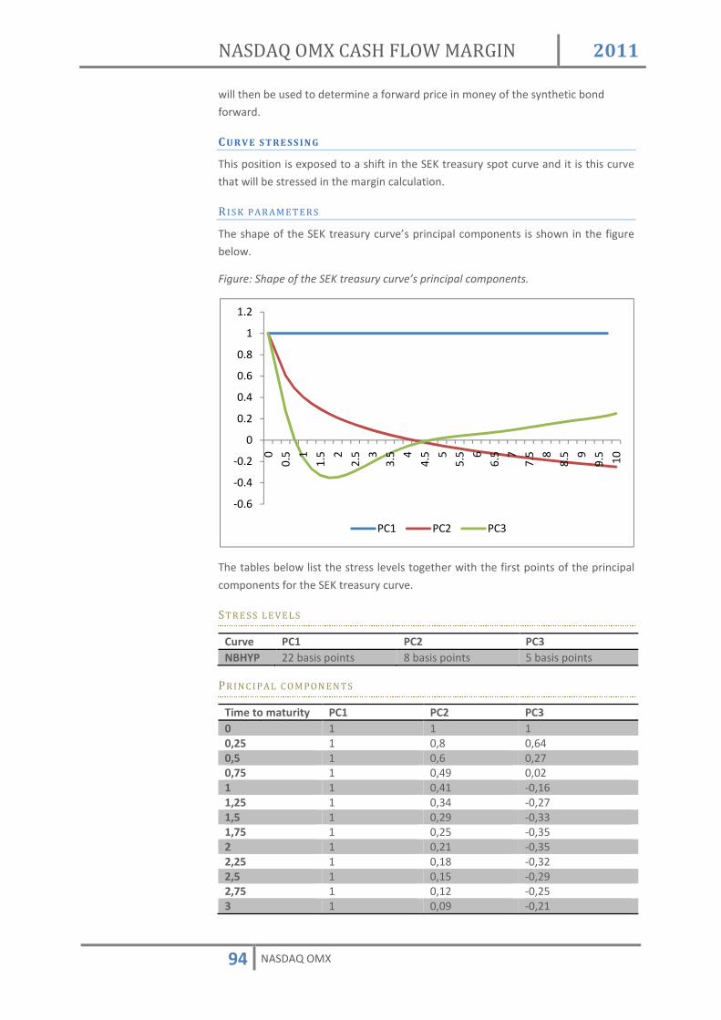
NASDAQ OMX CASH FLOW MARGIN 2011
94 NASDAQ OMX
will then be used to determine a forward price in money of the synthetic bond
forward.
C U R V E S T R E S S I N G
This position is exposed to a shift in the SEK treasury spot curve and it is this curve
that will be stressed in the margin calculation.
R I S K P A R A M E T E R S
The shape of the SEK treasury curve’s principal components is shown in the figure
below.
Figure: Shape of the SEK treasury curve’s principal components.
The tables below list the stress levels together with the first points of the principal
components for the SEK treasury curve.
ST R E S S L E V E L S
Curve PC1 PC2 PC3 NBHYP 22 basis points 8 basis points 5 basis points
PR I N C I P A L C O M P O N E N T S
Time to maturity PC1 PC2 PC3 0 1 1 1 0,25 1 0,8 0,64 0,5 1 0,6 0,27 0,75 1 0,49 0,02 1 1 0,41 -0,16 1,25 1 0,34 -0,27 1,5 1 0,29 -0,33 1,75 1 0,25 -0,35 2 1 0,21 -0,35 2,25 1 0,18 -0,32 2,5 1 0,15 -0,29 2,75 1 0,12 -0,25 3 1 0,09 -0,21
-0.6
-0.4
-0.2
0
0.2
0.4
0.6
0.8
1
1.2
00.
5 11.
5 22.
5 33.
5 44.
5 55.
5 66.
5 77.
5 88.
5 99.
5 10
PC1 PC2 PC3

NASDAQ OMX CASH FLOW MARGIN 2011
95 NASDAQ OMX
3,25 1 0,07 -0,16 3,5 1 0,05 -0,12
OF F I C I A L C U R V E S
NOMX will, on each trading day, bootstrap official yield curves that will be used to
price all cleared instruments. It is the official yield curves that will be stressed in the
margin calculations. In this example it is assumed that the official SEK treasury spot
curve look as in the figure below.
The table below lists the official swap spot and forward-forward rates for the
maturities that are relevant to the cash flows in the treasury cash flow table.
Equation (2) has been used to calculate the forward-forward rates,������� ����� from the spot rates� ������.
m i(0,m) f(0,m,m+i) 0,28767 1,757%
1,17808 2,162% ±�4 * 3�4j3]�X�X^mWm�4 * 4�l2l]�W�Um^�^²X�X�X^mWmW�Um^�^� � 4 3�3T[]
2,17808 2,523% ±�4 * 3�23[]�U�X^mWm�4 * 4�l2l]�W�Um^�^²X�U�X^mWmW�Um^�^� � 4 3�j_�]
3,17808 2,894% ±�4 * 3�ST_]���X^mWm�4 * 4�l2l]�W�Um^�^²X���X^mWmW�Um^�^� � 4 [���l]
The next step is to calculate a forward price quoted in yield for the deliverable bond.
The forward yield to maturity, Ò, is the solution of Equation(20). Note that the time
in this equation relates to the time between the expiration date of the forward and
the cash flow date.
��^�W�WWW�X U�UV�]�ÓÔÕÈÓÖÕ * ��^�W�WWW�X U��kW]�Ö×ÕÈÓÖÕ * XW��^�W�WWW�X ��WW^]�ØÕÙÕÈÓÖÕ ��^�W�WWW�X Ú�ÓÔÕÈÓÖÕ * ��^�W�WWW�X Ú�Ö×ÕÈÓÖÕ *XW��^�W�WWW�X Ú�ØÕÙÕÈÓÖÕ Û Ü 3�TlT]
0.00%
0.50%
1.00%
1.50%
2.00%
2.50%
3.00%
3.50%
0.25 0.75 1.25 1.75 2.25 2.75 3.25 3.75 4.25 4.75 5.25 5.75 6.25
treasury

NASDAQ OMX CASH FLOW MARGIN 2011
96 NASDAQ OMX
Equation (19) will be used to convert the yield into a price for the synthetic bond.
;º�» �3�TlT]� 4������� , �j]3�TlT] , ��4 * 3�TlT]�U � 4� * 4���4 * 3�TlT]����W��W UX�� 4��2l�S3_
ST R E S S E D C U R V E S
The first cash flow is a positive one and thus the worst scenario for that cash flow
will be that all short treasury spot rates goes up. However, the position’s cash flows
that are most distance are the ones that are derived from the underlying bond.
These are all negative cash flows and hence these positions are mainly exposed to a
downward shift in the treasury curve. If one considers all cash flows, the worst
outcome will be the scenario where the first two principal components are stressed
downwards and the third principal component is stressed upwards.
Figure: The worst scenario is when the treasury curve is stressed downward
Figure: Official treasury curve and stressed treasury curve
-0.30%
-0.25%
-0.20%
-0.15%
-0.10%
-0.05%
0.00%
0.05%
0.10%
0 0.25 0.5 0.75 1 1.25 1.5 1.75 2 2.25 2.5 2.75 3 3.25 3.5
PC1 PC2 PC3 Combined

NASDAQ OMX CASH FLOW MARGIN 2011
97 NASDAQ OMX
NOMX defines the principal components in a predefined number of nodes. The
distance between each node is in this example 0,25 years. A linear interpolation will
be used in order to determine the stress levels for the different maturities. This can
be seen in the table below.
Time to maturity
PC1 PC2 PC3
0 1 1 1 0,25 1 0,8 0,64
0,28767
1 ��S * ��j � ��S��2 � ��32 , ���3Sljl� ��32� ��ljTSj
��j_ * ��3l � ��j_��2 � ��32 , ���3Sljl� ��32� ��2S_32
0,5 1 0,6 0,27
0,75 1 0,49 0,02
1 1 0,41 -0,16
1,17808 1 ��_4 * ��[_ � ��_44�32 � 4 , �4�4lS�S � 4� ��[j�4_
���4j * ���3l * ��4j4�32 � 4 , �4�4lS�S � 4� ���3[S[j 1,25 1 0,34 -0,27 1,5 1 0,29 -0,33
1,75 1 0,25 -0,35
2 1 0,21 -0,35
2,17808 1 ��34 * ��4S � ��343�32 � 3 , �3�4lS�S � 3� ��4SSj[
���[2 * ���[3 * ��[23�32 � 3 , �3�4lS�S � 3� ���[3Sj[
2,25 1 0,18 -0,32
2,5 1 0,15 -0,29 2,75 1 0,12 -0,25
3 1 0,09 -0,21
3,17808 1 ���T * ���l � ���T[�32 � [ , �[�4lS�S� [� ���l2l2
���34 * ���4j * ��34[�32 � [ , �[�4lS�S � [� ���4l_[S 3,25 1 0,07 -0,16
3,5 1 0,05 -0,12
0.00%
0.50%
1.00%
1.50%
2.00%
2.50%
3.00%
3.50%
0.25 0.5 0.75 1 1.25 1.5 1.75 2 2.25 2.5 2.75 3 3.25 3.5
Spot Stressed

NASDAQ OMX CASH FLOW MARGIN 2011
98 NASDAQ OMX
After the SEK treasury spot rates have been stressed then Equation (2) is used to
update the SEK treasury forward-forward rates. The tables below list the official and
the stressed SEK treasury rates.
m i(0,m) i(0,m) (stressed)
0,28767 1,757% 4�l2l] � ��33] , 4 � ���S] , ljTSj * ���2], ��2S_32 4�2�2]
1,17808 2,162% 3�4j3] � ��33] , 4 � ���S] , ��[j�4_� ���2] , ��3[S[j 4�T�4]
2,17808 2,523% 3�23[] � ��33] , 4 � ���S] , ��4SSj[� ���2] , ��[3Sj[ 3�3l4]
3,17808 2,894% 3�ST_] � ��33] , 4 � ���S] , ���l2l2� ���2] , ��4l_[S 3�j2T]
m i(0,m) (stressed)
f(0,m,m+i) (stressed)
0,28767 1,505%
1,17808 1,901% ±�4 * 4�T�4]�X�X^mWm�4 * 4�2�2]�W�Um^�^²X�X�X^mWmW�Um^�^� � 4 3��[�]
2,17808 2,271% ±�4 * 3�3l4]�U�X^mWm�4 * 4�2�2]�W�Um^�^²X�U�X^mWmW�Um^�^� � 4 3�[ST]
3,17808 2,659% ±�4 * 3�j2T]���X^mWm�4 * 4�2�2]�W�Um^�^²X���X^mWmW�Um^�^� � 4 3�ll2]
S T R E S S E D NE T P R E S E N T V A L U E
Equation (28) is used to calculate a forward price quoted in yield for the deliverable
bond with the stressed forward-forward rates. The forward yield to maturity, ÒR�Ý\RR, is the solution of Equation (28). Note that the time in this equation relates to
the time between the expiration date of the forward and the cash flow date.
��^�W�WWW�X U�W�W]�ÓÔÕÈÓÖÕ * ��^�W�WWW�X U��mV]�Ö×ÕÈÓÖÕ * XW��^�W�WWW�X U�^^�]�ØÕÙÕÈÓÖÕ ��^�W�WWW�X ÚÞßàáÞÞ�ÓÔÕÈÓÖÕ * ��^�W�WWW�X ÚÞßàáÞÞ�Ö×ÕÈÓÖÕ *XW��^�W�WWW�X ÚÞßàáÞÞ�ØÕÙÕÈÓÖÕ Û Ü��â��� 3�l_2]
Equation (27) will be used to convert the stressed yield into a stressed price for the
synthetic bond.
;º�» �3�l_2]� 4������� , �j]3�l_2] , ��4 * 3�l_2]�U � 4� * 4���4 * 3�l_2]����W��W UX�� 4��j3�24_
The margin requirement is obtained by comparing the stressed price from the
stressed curve with the price obtained by the unstressed curve. Note that this is

NASDAQ OMX CASH FLOW MARGIN 2011
99 NASDAQ OMX
forward prices which have to be discounted back to today i.e. 2011-03-02 to get a
stressed net present value.
The market value will be calculated from equation (27) and is based on the
difference between the traded price (r) and today’s fixed price (rt). In this example it
is assumed that the traded price and the fixed price are equal. If, on the other hand,
the net present value is calculated with the stressed SEK treasury curve, then the
bond forward position’s margin requirement is obtained.
Market value ª«¬®�/� ¢¢]� ��ª«¬®�/� ¢¢]� �
NPV stressed 4�2�lS3�_���4 * 4�2�2]�W�Um^�^ � 4�j�324�_���4 * 4�2�2]�W�Um^�^ ��_jj�TST
Market value = SEK 0
Margin requirement = SEK -466 989

NASDAQ OMX CASH FLOW MARGIN 2011
100 NASDAQ OMX
APPENDICES APPENDIX I BOOTS TR APPI NG YI ELD CU RV ES USI NG CUBI C S PLIN ES NOMX applies a cubic spline bootstrapping methodology to obtain the yield curves.
This appendix describes the cubic spline bootstrapping methodology.
O B J E C T I V E
The objective is to find a discount function, ������� that prices all calibration
instruments correct and that is smooth and has a smooth first and second
derivative.
BA S I C A S S U M P T I O N S
The discount function is divided in a number of nodes, and it is assumed that it can
be expressed as a 3rd degree polynomial in between these nodes. This implies that
the discount function can be written as Equation (31).
������ +��� � * .��� � , �� ���� * 0��� � , �� ����/ +���� � , �� ����1 31
PR O B L E M
The problem is to find the coefficients�8i�ã � �di�ã � äi�ã� �i�ã. If these are found then
the discount function is defined on the interval�N���\» P. The discount function is
divided in x nodes, were x is the number of calibration instruments. Each node lay at
the end date of the calibration instrument’s underlying rate period. Equation (31)
gives four unknown coefficients per node interval, and this results in a total of 4 · x
unknown coefficients.
S O L U T I O N
PR I C E E Q U A T I O N S
The discount function must price all calibration instruments correct. The x number
of calibration instruments therefore give x price equations. The price equation will
look different depending on which type of instrument that is used as calibration
instrument.
B I L L S
Equation (32) can be used to relate the discount function to the price of a bill.
�����&�F� �� $.,M�h/��1C� , ������ /� 32
t� U�å is the actual number of days between t+2 and x, and 7ºis the bill’s yield.
B O N D S
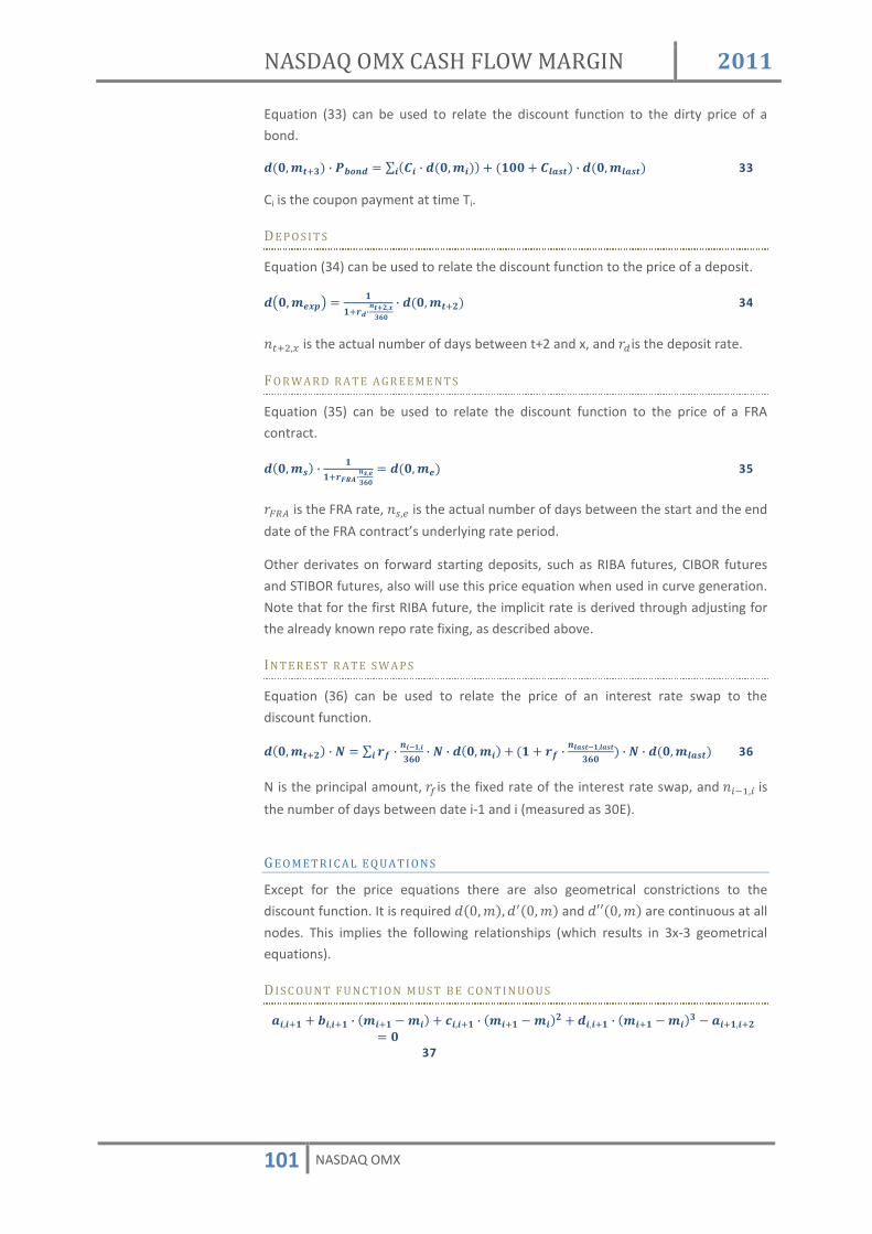
NASDAQ OMX CASH FLOW MARGIN 2011
101 NASDAQ OMX
Equation (33) can be used to relate the discount function to the dirty price of a
bond.
������ 1� , -.GM� æ �"� , ��������� * ���� * "J+)�� , �����J+)�� 33
Ci is the coupon payment at time Ti.
DE P O S I T S
Equation (34) can be used to relate the discount function to the price of a deposit.
�����&�F� �� $�,M�h/��1C� , ������ /� 34
t� U�å is the actual number of days between t+2 and x, and 7 is the deposit rate.
F O R W A R D R A T E A GR E E M E N T S
Equation (35) can be used to relate the discount function to the price of a FRA
contract.
�����)� , �� $qHr,M)�&1C� �����&� 35
7vwx is the FRA rate, tR�\ is the actual number of days between the start and the end
date of the FRA contract’s underlying rate period.
Other derivates on forward starting deposits, such as RIBA futures, CIBOR futures
and STIBOR futures, also will use this price equation when used in curve generation.
Note that for the first RIBA future, the implicit rate is derived through adjusting for
the already known repo rate fixing, as described above.
IN T E R E S T R A TE S W A P S
Equation (36) can be used to relate the price of an interest rate swap to the
discount function.
������ /� , D æ $� , M�!���1C� , D , ������� *� �� * $� , MJ+)�!��J+)�1C� � , D , �����J+)�� 36
N is the principal amount, 7ç is the fixed rate of the interest rate swap, and tiX�i is
the number of days between date i-1 and i (measured as 30E).
G E O M E T R I CA L E Q U A T I O N S
Except for the price equations there are also geometrical constrictions to the
discount function. It is required ������� �¿����� and �èè������are continuous at all
nodes. This implies the following relationships (which results in 3x-3 geometrical
equations).
D I S C O U N T F U N C T I O N M U S T B E C O N T I N U O U S
+��� � * .��� � , ��� � ���� * 0��� � , ��� � ����/ * ���� � , ��� � ����1 � +� ��� / � 37

NASDAQ OMX CASH FLOW MARGIN 2011
102 NASDAQ OMX
D I S C O U N T F U N C T I O N M U S T H A V E A C O N T I N U O U S D E R I V A T I V E
.��� � * / , 0��� � , ��� � ���� * 1 , ���� � , ��� � ����/ � .� ��� / � 38
D I S C O U N T F U N C T I O N M U S T H A V E A C O N T I N U O U S S E C O N D D E R I V A T I V E
/ , 0��� � * C , ���� ���� � ���� � / , 0� ��� / � 39
B O U N D A R Y C O N D I T I O N S
The following three boundary conditions are applied.
• The discount function is defined to start at 1 i.e. ������ 4.
+��� � 40
• The discount function is assumed to have a smooth start i.e. �èè����� 4.
0��� � 41
• The discount function is assumed to reach an equilibrium state i.e. ��¿¿����\» � �.
/ , 0&M���&M� * C , �&M���&M���&M� ��&M��� � 42
SY S T E M O F L I N E A R E Q U A T I O N S
The price equations, geometrical equations and boundary conditions result in a total
of 4 · x equations. These can be solved for all unknown coefficients��8i�ã � �di�ã � äi�ã ��i�ã. When the coefficients have been found then Equation (31) can be used to
calculate the discount function for any time to maturity on the interval�N���\» P.

NASDAQ OMX CASH FLOW MARGIN 2011
103 NASDAQ OMX
APPENDIX II PRIN CIP A L CO MPO N EN TS A NA LYSI S NOMX will stress each yield curve with its first three principal components. The
principal component analysis will be performed outside of the GENIUM INET system
and the principal components together with their stress levels will be entered into
GENIUM INET as risk parameters. This appendix describes the principal component
analysis.
O B J E C T I V E
The objective is to find independent (uncorrelated) moves of a yield curve; these
will later be used to simulate changes to the yield curve.
IN P U T D A T A
NOMX defines the yield curves as interest rate values at different times to
maturities (nodes).
Time to maturity m0 … mi … mend Spot rate i(t,m0) … i(t,mi) … i(t,mend)
The input data to the principal components analysis is a time series of historical
changes to these node values.
Date m0 … mend ti é��`i � �W� � ��`iX� �W�é … é��`i � �\» � � ��`iX� �\» �é ti-1 é��`iX� �W� � ��`iU� �W�é … é��`iX� �\» � � ��`iU� �\» �é … … … … ti-500 é��`i�WW� �W� � ��`i�WX� �W�é … é��`i�WW��\» � � ��`i�WX� �\» �é
DE F I N I T I O N S
C O V A R I A N C E M A T R I X
The covariance matrix contains information on each node’s historical variance as
well as the covariance between the different nodes. The covariance matrix is
defined accordingly.
"êë��� ì� æ����íî ���ì�ïî �M 43
xi is the daily change of node i, xj is the daily change of node j, and n is the total
number of observations.
When performing the principal components analysis it is important that the input
data is arranged so that the means ðñî and ðòî are zero5. If this is not correct then the
means must be removed from the time series before the analysis proceeds.
5 Please see Jolliffe, I.T. Principal Components Analysis, 2nd edition, Springer series in statistics

NASDAQ OMX CASH FLOW MARGIN 2011
104 NASDAQ OMX
PR I N C I P A L C O M P O N E N T S
The principal components are defined as the eigenvectors, λ, to the covariance
matrix.
"êëóôôôôôôôõ , ö' ÷ , ö' 44
The eigenvectors are orthogonal i.e. independent (uncorrelated). An eigenvector’s
eigenvalue, σ, reveals how much of the curve’s total variance that is explained by
this eigenvector. It should be noted that this definition implies that the principal
components are in fact lists of changes to the interest rate values at the nodes.
Time to maturity m0 … mi … mend Spot rate change 1 … 0,9 … 0,4
PR O B L E M
The first problem is to find the eigenvalues, σ, to the covariance matrix. This is done
by solving Equation (35). I in Equation (35) stands for the identification matrix.
®Â��"êëóôôôôôôôõ � ÷ , �ø� � 45
When the eigenvalues are found, then each of them can be inserted into Equation
(44), resulting in a system of linear equations that can be solved for their
corresponding eigenvectors, λ.
S O L U T I O N
If the yield curve is defined on x nodes, then the covariance matrix will have
size�ð , ð. Equation (45) will then result in x eigenvalues (assuming no doublets) and
hence also x eigenvectors/principal components.
If the size of all eigenvalues is compared, then it is possible to determine the
importance of each principal component. The table below shows the relative
importance of the SEK swap curve’s first seven principal components.
Principal component PC1 PC2 PC3 PC4 PC5 PC6 PC7 Explanation factor 76,5% 12,7% 5,1% 2,0% 0,9% 0,7% 0,4%
The Risk parameters are dependent on the principal components. From the
principal components analysis the eigenvectors are by definition orthonormal i.e.
orthogonal vectors with magnitude 1. NASDAQ OMX has chosen to scale the
eigenvectors/principal components and that will affect both the magnitude of the
eigenvector and the risk parameter i.e. the greater the magnitude the lower the risk
parameter. However, the direction of the eigenvector will not change which means
that the actual stress (Risk parameter *�;¾) will not change depending of the
magnitude of the principal components

NASDAQ OMX CASH FLOW MARGIN 2011
105 NASDAQ OMX
Figure: First five scaled principal components of the SEK swap curve.
-1.5
-1
-0.5
0
0.5
1
1.5
0.25
0.75
1.25
1.75
2.25
2.75
3.25
3.75
4.25
4.75
5.25
5.75
6.25
6.75
7.25
7.75
8.25
8.75
9.25
9.75
PC1 PC2 PC3 PC4 PC5
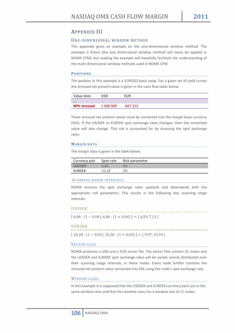
NASDAQ OMX CASH FLOW MARGIN 2011
106 NASDAQ OMX
APPENDIX III ON E-DI MEN SION AL WI NDOW MET HO D This appendix gives an example on the one-dimensional window method. The
example is fictive (the one dimensional window method will never be applied in
NOMX CFM), but reading the example will hopefully facilitate the understanding of
the multi-dimensional window methods used in NOMX CFM.
PO S I T I O N S
The position in this example is a EURUSD basis swap. For a given set of yield curves
the stressed net present value is given in the cash flow table below.
Value date USD EUR … … … NPV stressed 1 000 000 -667 315
These stressed net present values must be converted into the margin base currency
(SEK). If the USDSEK or EURSEK spot exchange rates changes, then the converted
value will also change. This risk is accounted for by stressing the spot exchange
rates.
MA R G I N D A T A
The margin data is given in the table below.
Currency pair Spot rate Risk parameter USDSEK 6,86 4% EURSEK 10,28 3%
SC A N N I N G R A N G E IN T E R VA L S
NOMX stresses the spot exchange rates upwards and downwards with the
appropriate risk parameters. This results in the following two scanning range
intervals.
USDSE K
N�j�Sj , �4 � ���_�� j�Sj , �4 * ���_��P N�j�2T� l�4[�P EURSEK
N�4��3S , �4 � ���[�� 4��3S , �4 * ���[��P N�T�Tl� 4��2T�P VE C T O R F I L E S
NOMX produces a USD and a EUR vector file. The vector files contain 31 nodes and
the USDSEK and EURSEK spot exchange rates will be varied, evenly distributed over
their scanning range intervals, in these nodes. Every node further contains the
stressed net present value converted into SEK using the node’s spot exchange rate.
W I N D O W C L A S S
In this example it is supposed that the USDSEK and EURSEK currency pairs are in the
same window class and that this window class has a window size of 11 nodes.

NASDAQ OMX CASH FLOW MARGIN 2011
107 NASDAQ OMX
O N E -D I M E N S I O N A L W I N D O W M E T H O D
The one-dimensional window method starts by listing the USD and EUR vector files
next to each other and by creating a “USD, EUR result vector” (refer to the figure
below).
W I N D O W S T A R T S I N N O D E 1
A window of 11 nodes is then placed in the top node of the vector files. The window
represent the maximum amount that the USDSEK and EURSEK spot exchange rates
are anticipated to deviate from each other. The value at node 1 of the result vector
is the sum of the worst outcomes from the nodes in the USD and EUR vector files
that lay inside of the window.
In this example this is node 6 of the USD vector file (i.e. that the USDSEK spot rate
goes up to 7,04) and node 1 of the EUR vector file (i.e. that EURSEK spot rate goes
up to 10,59). This combined result is entered into node 1 of the result vector.
Figure: A window starts at the top node of the vector files. The value in the result
vector is the sum of the worst outcome within the window.
USD vector file
EUR vector file
USD, EUR result vector
Node USDSEK NPV (SEK) Node EURSEK NPV (SEK) Node USDSEK EURSEK NPV (SEK)
1 7,13 7 134 400 1 10,59 -7 065 800 1 7,04 10,59 -22 867
2 7,12 7 116 107 2 10,57 -7 052 080 2 3 7,10 7 097 813 3 10,55 -7 038 360 3 4 7,08 7 079 520 4 10,53 -7 024 640 4 5 7,06 7 061 227 5 10,51 -7 010 920 5 6 7,04 7 042 933 6 10,49 -6 997 200 6
7 7,02 7 024 640 7 10,47 -6 983 480 7 8 7,01 7 006 347 8 10,44 -6 969 760 8 9 6,99 6 988 053 9 10,42 -6 956 040 9 10 6,97 6 969 760 10 10,40 -6 942 320 10 11 6,95 6 951 467 11 10,38 -6 928 600 11 12 6,93 6 933 173 12 10,36 -6 914 880 12 13 6,91 6 914 880 13 10,34 -6 901 160 13 14 6,90 6 896 587 14 10,32 -6 887 440 14 15 6,88 6 878 293 15 10,30 -6 873 720 15 16 6,86 6 860 000 16 10,28 -6 860 000 16 17 6,84 6 841 707 17 10,26 -6 846 280 17 18 6,82 6 823 413 18 10,24 -6 832 560 18 19 6,81 6 805 120 19 10,22 -6 818 840 19 20 6,79 6 786 827 20 10,20 -6 805 120 20 21 6,77 6 768 533 21 10,18 -6 791 400 21 22 6,75 6 750 240 22 10,16 -6 777 680 22 23 6,73 6 731 947 23 10,14 -6 763 960 23 24 6,71 6 713 653 24 10,12 -6 750 240 24 25 6,70 6 695 360 25 10,09 -6 736 520 25 26 6,68 6 677 067 26 10,07 -6 722 800 26 27 6,66 6 658 773 27 10,05 -6 709 080 27 28 6,64 6 640 480 28 10,03 -6 695 360 28 29 6,62 6 622 187 29 10,01 -6 681 640 29 30 6,60 6 603 893 30 9,99 -6 667 920 30 31 6,59 6 585 600 31 9,97 -6 654 200 31

NASDAQ OMX CASH FLOW MARGIN 2011
108 NASDAQ OMX
W I N D O W S L I D E S D O W N
The window will slide down all 31 nodes of the vector files. The value in the result
vector is always the sum of the worst outcomes within the window.
At note 16 this is equal the value from node 21 of the USD vector file (i.e. that the
USDSEK spot rate goes down to 6,77) plus the value from node 11 of the EUR vector
file (i.e. that the EURSEK spot rate goes up to 10,38).
Figure: The window will slide down all 31 nodes of the vector files.
USD vector file
EUR vector file
USD, EUR result vector
Node USDSEK NPV (SEK) Node EURSEK NPV (SEK) Node USDSEK EURSEK NPV (SEK) 1 7,13 7 134 400 1 10,59 -7 065 800 1 7,04 10,59 -22 867 2 7,12 7 116 107 2 10,57 -7 052 080 2 7,02 10,59 -41 160 3 7,10 7 097 813 3 10,55 -7 038 360 3 7,01 10,59 -59 453 4 7,08 7 079 520 4 10,53 -7 024 640 4 6,99 10,59 -77 747 5 7,06 7 061 227 5 10,51 -7 010 920 5 6,97 10,59 -96 040 6 7,04 7 042 933 6 10,49 -6 997 200 6 6,95 10,59 -114 333 7 7,02 7 024 640 7 10,47 -6 983 480 7 6,93 10,57 -118 907 8 7,01 7 006 347 8 10,44 -6 969 760 8 6,91 10,55 -123 480 9 6,99 6 988 053 9 10,42 -6 956 040 9 6,90 10,53 -128 053 10 6,97 6 969 760 10 10,40 -6 942 320 10 6,88 10,51 -132 627
11 6,95 6 951 467 11 10,38 -6 928 600 11 6,86 10,49 -137 200 12 6,93 6 933 173 12 10,36 -6 914 880 12 6,84 10,47 -141 773 13 6,91 6 914 880 13 10,34 -6 901 160 13 6,82 10,44 -146 347 14 6,90 6 896 587 14 10,32 -6 887 440 14 6,81 10,42 -150 920 15 6,88 6 878 293 15 10,30 -6 873 720 15 6,79 10,40 -155 493
16 6,86 6 860 000 16 10,28 -6 860 000 16 6,77 10,38 -160 067
17 6,84 6 841 707 17 10,26 -6 846 280 18 6,82 6 823 413 18 10,24 -6 832 560 19 6,81 6 805 120 19 10,22 -6 818 840 20 6,79 6 786 827 20 10,20 -6 805 120 21 6,77 6 768 533 21 10,18 -6 791 400
22 6,75 6 750 240 22 10,16 -6 777 680 23 6,73 6 731 947 23 10,14 -6 763 960 24 6,71 6 713 653 24 10,12 -6 750 240 25 6,70 6 695 360 25 10,09 -6 736 520 26 6,68 6 677 067 26 10,07 -6 722 800 27 6,66 6 658 773 27 10,05 -6 709 080 28 6,64 6 640 480 28 10,03 -6 695 360 29 6,62 6 622 187 29 10,01 -6 681 640 30 6,60 6 603 893 30 9,99 -6 667 920 31 6,59 6 585 600 31 9,97 -6 654 200
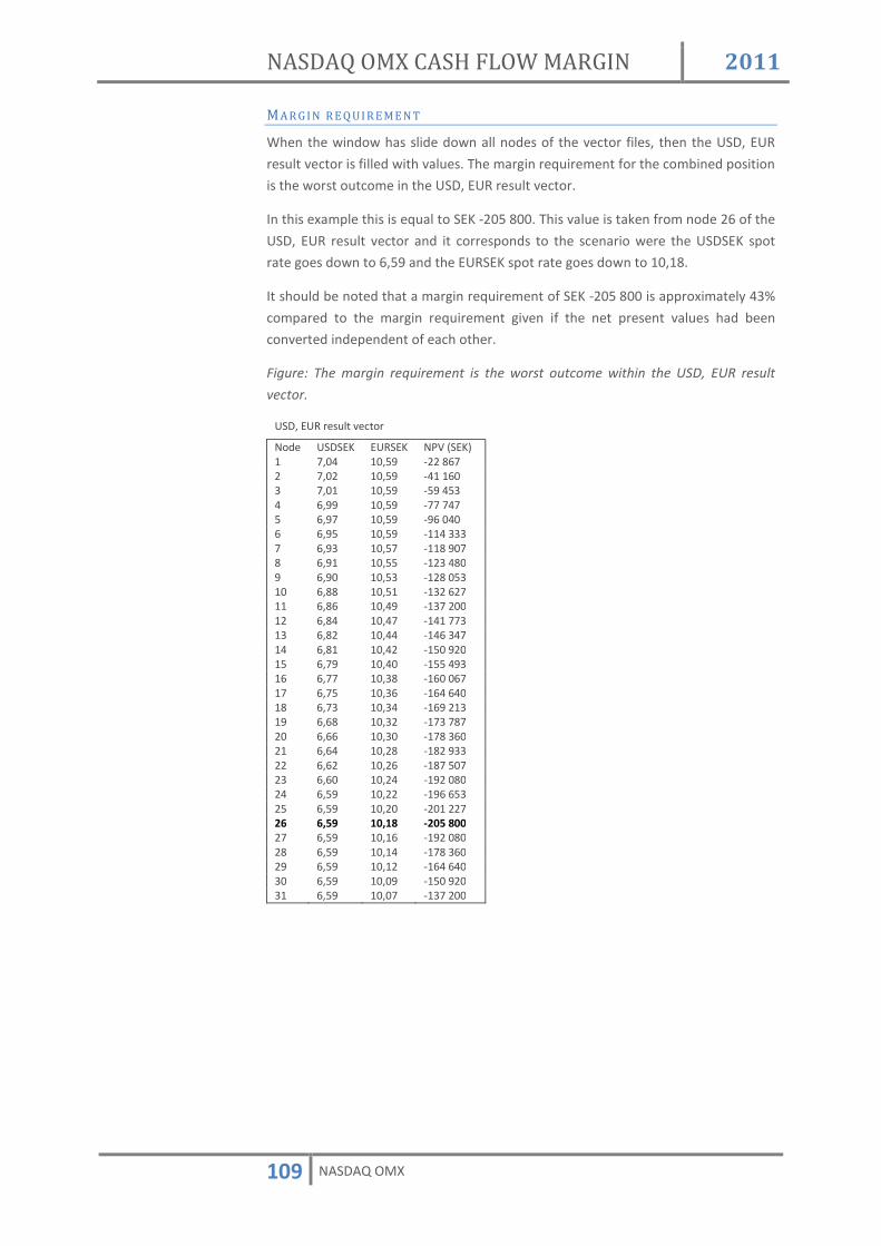
NASDAQ OMX CASH FLOW MARGIN 2011
109 NASDAQ OMX
M A R G I N R E Q U I R E ME N T
When the window has slide down all nodes of the vector files, then the USD, EUR
result vector is filled with values. The margin requirement for the combined position
is the worst outcome in the USD, EUR result vector.
In this example this is equal to SEK -205 800. This value is taken from node 26 of the
USD, EUR result vector and it corresponds to the scenario were the USDSEK spot
rate goes down to 6,59 and the EURSEK spot rate goes down to 10,18.
It should be noted that a margin requirement of SEK -205 800 is approximately 43%
compared to the margin requirement given if the net present values had been
converted independent of each other.
Figure: The margin requirement is the worst outcome within the USD, EUR result
vector.
USD, EUR result vector
Node USDSEK EURSEK NPV (SEK) 1 7,04 10,59 -22 867 2 7,02 10,59 -41 160 3 7,01 10,59 -59 453 4 6,99 10,59 -77 747 5 6,97 10,59 -96 040 6 6,95 10,59 -114 333 7 6,93 10,57 -118 907 8 6,91 10,55 -123 480 9 6,90 10,53 -128 053 10 6,88 10,51 -132 627 11 6,86 10,49 -137 200 12 6,84 10,47 -141 773 13 6,82 10,44 -146 347 14 6,81 10,42 -150 920 15 6,79 10,40 -155 493 16 6,77 10,38 -160 067 17 6,75 10,36 -164 640 18 6,73 10,34 -169 213 19 6,68 10,32 -173 787 20 6,66 10,30 -178 360 21 6,64 10,28 -182 933 22 6,62 10,26 -187 507 23 6,60 10,24 -192 080 24 6,59 10,22 -196 653 25 6,59 10,20 -201 227 26 6,59 10,18 -205 800 27 6,59 10,16 -192 080 28 6,59 10,14 -178 360 29 6,59 10,12 -164 640 30 6,59 10,09 -150 920 31 6,59 10,07 -137 200

NASDAQ OMX CASH FLOW MARGIN 2011
110 NASDAQ OMX
APPENDIX IV A G UID E TO MAR GIN R EPLI CATION USIN G INT ERFA CE FI LES Through the API, NOMX offers access to risk cubes which can be used to replicate
the margin calculation exactly. These risk cubes are also available as interface files.
In this appendix we will focus on information from queries EQ10, JQ16, JQ40 and
JQ41. With this information CFM margin can be fully replicated.
EQ10 ( I N T E R F A C E F I L E * .YCT)
This query answer/interface file contains information regarding the curves used in
the CFM calculation. When replicating margins we are foremost interested in the
information it holds about which curves are correlated. The curve identification
codes are found in the first column, and the corresponding window group (if any)
can be found in the second column.
JQ 16 (IN T E R F A C E F I L E * .CCT)
This query answer/interface file describes the different window groups. Most
importantly, in the third, fourth and fifth column the window size in each principal
component dimension is found. In the second column, the upper window group (if
any) can be found.
JQ 40 ( I N T E R F A C E F I L E * . R C T)
This query answer/interface file contains instrument series specific information
used in the margin calculation. The file is only available for instruments with
standardized series. For OTC-style contracts, see JQ41 below.
The first row contains metadata. Please study the example below, for the
instrument series FRAO12.
1 3 18 0 2033 11891 0 2 …
… SWAP_SEK SWAP_SEK
7 TSN
The following data rows each represent one of the curve scenarios. If, for example,
the scanning range is 5 in each principal component dimension, there will be 5*5*5
= 125 rows.
Exchange Market Instr Group Modifier Commodity
Number of decimals in
Margin Value
Expiration Date Strike Price
Primary Curve Id Secondary Curve Number of decimals in Discount Factor
Primary Curve Correlation Cube Id
Secondary Curve Correlation Cube Id Closing Date
Margin Class

NASDAQ OMX CASH FLOW MARGIN 2011
111 NASDAQ OMX
These data rows can be divided into three parts;
• the first three columns described the stress applied to the yield curve,
Where 0 indicates that the PC was stressed to its minimum level. If the
resolution is 5 in each PC, 4 indicates that the PC was stressed to its
maximum leve, and 2 indicates no stress in the PC.
•
•
•
• The next six columns describe the NPV for the “unknown” part of the
instrument. This means the floating cash flow of a FRA, and the bond cash
flows of a bond forward. NB, this is a NPV and does not need to be
discounted further. The six columns represent the six combinations of
whether the position is long or short, and of whether the calculations are
made under a low, mid or high volatility stress. Note that for all
instruments except options, it suffices to use the first two of these six
columns. When interpreting the figures, the field Number of Decimals in
Margin Value from the meta data row has to be used. In this example it is
2, meaning that the NPV of the floating cash flow in one (1) long position in
the FRAO12 in scenario number 1 is 6569,33 SEK.
0 0 0 0 0 1 0 0 2 0 0 3 0 0 4 0 1 0 0 1 1 0 1 2 0 1 3 0 1 4 0 2 0 … …. …
656933 -656933 656933 -656933 656933 -656933 648636 -648636 648636 -648636 648636 -648636 640375 -640375 640375 -640375 640375 -640375 632120 -632120 632120 -632120 632120 -632120 623876 -623876 623876 -623876 623876 -623876 670887 -670887 670887 -670887 670887 -670887 662619 -662619 662619 -662619 662619 -662619 654348 -654348 654348 -654348 654348 -654348
… … … … … …
Stress in each principal component - PC1 PC2 PC3
Scenarios
Scenarios
Volatility: Low Low Mid Mid High High
Position: Long Short Long Short Long Short

NASDAQ OMX CASH FLOW MARGIN 2011
112 NASDAQ OMX
• The last two columns contain the discount factors used to calculate the
NPV of the contracted cash flow for long and short positions respectively.
Since the contracted rate depends on when the contract was entered, it is
left to the replicating agent to determine the undiscounted contracted cash
flow. When interpreting these figures, remember to use the field Number
of Decimals in Discount Function in the first meta data row. In this example
the number of decimals in the discount function is 7, so the discount
function for a long position in scenario 1 would be 0,9747635.
JQ40 is clearing house specific. Different members will get the same response from
JQ40, since it covers the margin calculations of standardized contracts. When it
comes to cleared OTC derivatives, whose contract details vary greatly between
different trades, member specific risk cubes / interface files are needed. This need is
covered by JQ41
JQ 41 (IN T E R F A C E F I L E * .CRV)
This query answer/interface file contains margin calculation information for cleared
OTC-trades, such as repos and swaps. The answer/file has one meta data row per
curve, one per trade, and thereafter one row for each scenario (which currently
makes 2 + 125 = 127 rows), multiplied by the number of cleared OTC-trades.
The metadata rows contain the information needed to identify the trade and to
interpret the scenario margin figures. The first of these rows is similar in design to
the metadata row in JQ40. The second metadata row contains the clearing account
code and the trade number.
The following data rows each represent one of the curve scenarios. If, for example,
the scanning range is 5 in each principal component dimension, there will be 5*5*5
= 125 rows per trade. There are six columns in each row, the first three describing
the combination of principal component stress in that specific scenario. The three
rightmost columns represent the NPV for the trade under three volatility regimes.
Notice that if the cleared trade is not an option, the NPV will be the same for all
three of the rightmost columns.
R E P L I C A T I N G N A K E D M A R G I N
Naked margin in CFM means the margin that is the result of one position or trade
being stressed in isolation. To replicate the naked margin follow these steps:
• For positions in standardized contracts, first calculate the contracted cash
flow. Then use the appropriate discount factor in JQ40 to calculate its NPV
in each curve scenario.
• For positions in standardized contracts, then calculate the “unknown” part
of the instrument. For FRAs this means the floating cash flow, for bond
forwards this means the NPV of the bond cash flows. This is done through
multiplying the value in the corresponding column ( long or short) with the
number of contracts in the net position, after dividing it with 10^(Number
of decimals in Margin Value).

NASDAQ OMX CASH FLOW MARGIN 2011
113 NASDAQ OMX
• For positions in standardized contracts, then calculate the total NPV for
each scenario by adding the two values above. The vector that is the result
we shall hereafter refer to as the stressed NPV vector.
• For OTC-trades, all the information needed to create the stressed NPV
vector can be found in the Margin Value columns in JQ 41, after dividing
them with 10^(Number of decimals in Margin Value).
• Finally, we can now find the naked margin per position/trade by choosing
the lowest value from the stressed NPV vector.
• NB, for derivatives where both the primary and secondary curves are used
for discounting, (e.g. repos and bond forwards) and where these curves are
different, one needs to take the worst of all NPVs of the contracted rate
and the worst of all NPVs of the bond cash flows, and add these together to
get the naked margin.
R E P L I C A T I N G M A R G I N
The correlation benefits in CFM can be said to occur on two levels.
On a curve level, there is a strong built-in correlation, which applies to all positions
and trades priced against the same curve.
On an inter curve level, there is the possibility of configuring a correlation in terms
of putting a limit on how much the applied stress can vary for curves within the
same window group. The theoretical workings have been described above, here we
will focus on how to achieve this effect with the help of the interface files.
The first step in replicating the margin is to aggregate all trades and positions that
are priced against the same curve. This is done by creating one stressed NPV vector
per curve, by adding together all of the stressed NPV vectors for the clients
positions and trades that are margined against this curve. We hereafter call this
aggregated vector the curve stressed NPV vector.
The second step of applying the correlation in between curves requires more
attention to detail. One needs to perform the shifting of a smaller cube
(representing the size of the window group) within a larger cube (representing the
total set of stress scenarios), but in just one dimension (in the set of stressed NPV
vectors). What is required is a method that translates the set of neighboring nodes
in a certain node of the cube, to rows in the vector file.

NASDAQ OMX CASH FLOW MARGIN 2011
114 NASDAQ OMX
Below is the description of a function, which can be called recursively to solve this
problem - finding the window group members for row n in the the stressed NPV
vector for a scenario space of size X*Y*Z, and a correlation window group of size
x*y*z. X, Y, Z and x, y, z are all odd numbers. The list of scenarios is ordered in the
same way as in the interface files, that is starting from negative stress in PC1 and
ending with positive stress in PC3.
On the following pages, also find a list of which rows that are neighbors to a certain
row in a framework where the total number of scenarios are 125 (5*5*5) and the
size of the window correlation cube is 27 (3*3*3).
function [ neighbours ] = neighbours( n, w_size, step , mod) neighbours = []; %Loop through the list of rows for i=1:size(n,2)
%find the "level" of the current row, to be able to distinguish %points outside the cube level = floor((n(i)-1)/mod); %find the neighbours in this dimension w = [-(w_size-1)/2:1:(w_size-1)/2]; new_neighbours = n(i) + step*w; %remove the neighbours which fall outside the given "level" new_neighours = new_neighbours(floor((new_neighbours-1)/mod) == level); neighbours = [neighbours, new_neighours]; end end scenarios = neighbours( neighbours( neighbours(n,z,1,Z)...
,y,Z,Y*Z)… ,x,Y*Z,X*Y*Z);

NASDAQ OMX CASH FLOW MARGIN 2011
115 NASDAQ OMX
Row Rows that are neighbours in a 3*3*3 correlation cube
1 1, 2, 6, 7, 26, 27, 31, 32 2 1, 2, 3, 6, 7, 8, 26, 27, 28, 31, 32, 33 3 2, 3, 4, 7, 8, 9, 27, 28, 29, 32, 33, 34 4 3, 4, 5, 8, 9, 10, 28, 29, 30, 33, 34, 35 5 4, 5, 9, 10, 29, 30, 34, 35 6 1, 2, 6, 7, 11, 12, 26, 27, 31, 32, 36, 37 7 1, 2, 3, 6, 7, 8, 11, 12, 13, 26, 27, 28, 31, 32, 33, 36, 37, 38 8 2, 3, 4, 7, 8, 9, 12, 13, 14, 27, 28, 29, 32, 33, 34, 37, 38, 39 9 3, 4, 5, 8, 9, 10, 13, 14, 15, 28, 29, 30, 33, 34, 35, 38, 39, 40
10 4, 5, 9, 10, 14, 15, 29, 30, 34, 35, 39, 40 11 6, 7, 11, 12, 16, 17, 31, 32, 36, 37, 41, 42 12 6, 7, 8, 11, 12, 13, 16, 17, 18, 31, 32, 33, 36, 37, 38, 41, 42, 43 13 7, 8, 9, 12, 13, 14, 17, 18, 19, 32, 33, 34, 37, 38, 39, 42, 43, 44 14 8, 9, 10, 13, 14, 15, 18, 19, 20, 33, 34, 35, 38, 39, 40, 43, 44, 45 15 9, 10, 14, 15, 19, 20, 34, 35, 39, 40, 44, 45 16 11, 12, 16, 17, 21, 22, 36, 37, 41, 42, 46, 47 17 11, 12, 13, 16, 17, 18, 21, 22, 23, 36, 37, 38, 41, 42, 43, 46, 47, 48 18 12, 13, 14, 17, 18, 19, 22, 23, 24, 37, 38, 39, 42, 43, 44, 47, 48, 49 19 13, 14, 15, 18, 19, 20, 23, 24, 25, 38, 39, 40, 43, 44, 45, 48, 49, 50 20 14, 15, 19, 20, 24, 25, 39, 40, 44, 45, 49, 50 21 16, 17, 21, 22, 41, 42, 46, 47 22 16, 17, 18, 21, 22, 23, 41, 42, 43, 46, 47, 48 23 17, 18, 19, 22, 23, 24, 42, 43, 44, 47, 48, 49 24 18, 19, 20, 23, 24, 25, 43, 44, 45, 48, 49, 50 25 19, 20, 24, 25, 44, 45, 49, 50 26 1, 2, 6, 7, 26, 27, 31, 32, 51, 52, 56, 57 27 1, 2, 3, 6, 7, 8, 26, 27, 28, 31, 32, 33, 51, 52, 53, 56, 57, 58 28 2, 3, 4, 7, 8, 9, 27, 28, 29, 32, 33, 34, 52, 53, 54, 57, 58, 59 29 3, 4, 5, 8, 9, 10, 28, 29, 30, 33, 34, 35, 53, 54, 55, 58, 59, 60 30 4, 5, 9, 10, 29, 30, 34, 35, 54, 55, 59, 60 31 1, 2, 6, 7, 11, 12, 26, 27, 31, 32, 36, 37, 51, 52, 56, 57, 61, 62 32 1, 2, 3, 6, 7, 8, 11, 12, 13, 26, 27, 28, 31, 32, 33, 36, 37, 38, 51, 52, 53, 56, 57, 58, 61, 62, 63 33 2, 3, 4, 7, 8, 9, 12, 13, 14, 27, 28, 29, 32, 33, 34, 37, 38, 39, 52, 53, 54, 57, 58, 59, 62, 63, 64 34 3, 4, 5, 8, 9, 10, 13, 14, 15, 28, 29, 30, 33, 34, 35, 38, 39, 40, 53, 54, 55, 58, 59, 60, 63, 64, 65 35 4, 5, 9, 10, 14, 15, 29, 30, 34, 35, 39, 40, 54, 55, 59, 60, 64, 65 36 6, 7, 11, 12, 16, 17, 31, 32, 36, 37, 41, 42, 56, 57, 61, 62, 66, 67 37 6, 7, 8, 11, 12, 13, 16, 17, 18, 31, 32, 33, 36, 37, 38, 41, 42, 43, 56, 57, 58, 61, 62, 63, 66, 67, 68 38 7, 8, 9, 12, 13, 14, 17, 18, 19, 32, 33, 34, 37, 38, 39, 42, 43, 44, 57, 58, 59, 62, 63, 64, 67, 68, 69 39 8, 9, 10, 13, 14, 15, 18, 19, 20, 33, 34, 35, 38, 39, 40, 43, 44, 45, 58, 59, 60, 63, 64, 65, 68, 69, 70 40 9, 10, 14, 15, 19, 20, 34, 35, 39, 40, 44, 45, 59, 60, 64, 65, 69, 70 41 11, 12, 16, 17, 21, 22, 36, 37, 41, 42, 46, 47, 61, 62, 66, 67, 71, 72 42 11, 12, 13, 16, 17, 18, 21, 22, 23, 36, 37, 38, 41, 42, 43, 46, 47, 48, 61, 62, 63, 66, 67, 68, 71, 72, 73 43 12, 13, 14, 17, 18, 19, 22, 23, 24, 37, 38, 39, 42, 43, 44, 47, 48, 49, 62, 63, 64, 67, 68, 69, 72, 73, 74 44 13, 14, 15, 18, 19, 20, 23, 24, 25, 38, 39, 40, 43, 44, 45, 48, 49, 50, 63, 64, 65, 68, 69, 70, 73, 74, 75 45 14, 15, 19, 20, 24, 25, 39, 40, 44, 45, 49, 50, 64, 65, 69, 70, 74, 75 46 16, 17, 21, 22, 41, 42, 46, 47, 66, 67, 71, 72 47 16, 17, 18, 21, 22, 23, 41, 42, 43, 46, 47, 48, 66, 67, 68, 71, 72, 73 48 17, 18, 19, 22, 23, 24, 42, 43, 44, 47, 48, 49, 67, 68, 69, 72, 73, 74 49 18, 19, 20, 23, 24, 25, 43, 44, 45, 48, 49, 50, 68, 69, 70, 73, 74, 75 50 19, 20, 24, 25, 44, 45, 49, 50, 69, 70, 74, 75 51 26, 27, 31, 32, 51, 52, 56, 57, 76, 77, 81, 82 52 26, 27, 28, 31, 32, 33, 51, 52, 53, 56, 57, 58, 76, 77, 78, 81, 82, 83 53 27, 28, 29, 32, 33, 34, 52, 53, 54, 57, 58, 59, 77, 78, 79, 82, 83, 84 54 28, 29, 30, 33, 34, 35, 53, 54, 55, 58, 59, 60, 78, 79, 80, 83, 84, 85 55 29, 30, 34, 35, 54, 55, 59, 60, 79, 80, 84, 85 56 26, 27, 31, 32, 36, 37, 51, 52, 56, 57, 61, 62, 76, 77, 81, 82, 86, 87 57 26, 27, 28, 31, 32, 33, 36, 37, 38, 51, 52, 53, 56, 57, 58, 61, 62, 63, 76, 77, 78, 81, 82, 83, 86, 87, 88 58 27, 28, 29, 32, 33, 34, 37, 38, 39, 52, 53, 54, 57, 58, 59, 62, 63, 64, 77, 78, 79, 82, 83, 84, 87, 88, 89 59 28, 29, 30, 33, 34, 35, 38, 39, 40, 53, 54, 55, 58, 59, 60, 63, 64, 65, 78, 79, 80, 83, 84, 85, 88, 89, 90 60 29, 30, 34, 35, 39, 40, 54, 55, 59, 60, 64, 65, 79, 80, 84, 85, 89, 90 61 31, 32, 36, 37, 41, 42, 56, 57, 61, 62, 66, 67, 81, 82, 86, 87, 91, 92 62 31, 32, 33, 36, 37, 38, 41, 42, 43, 56, 57, 58, 61, 62, 63, 66, 67, 68, 81, 82, 83, 86, 87, 88, 91, 92, 93 63 32, 33, 34, 37, 38, 39, 42, 43, 44, 57, 58, 59, 62, 63, 64, 67, 68, 69, 82, 83, 84, 87, 88, 89, 92, 93, 94 64 33, 34, 35, 38, 39, 40, 43, 44, 45, 58, 59, 60, 63, 64, 65, 68, 69, 70, 83, 84, 85, 88, 89, 90, 93, 94, 95

NASDAQ OMX CASH FLOW MARGIN 2011
116 NASDAQ OMX
65 34, 35, 39, 40, 44, 45, 59, 60, 64, 65, 69, 70, 84, 85, 89, 90, 94, 95 66 36, 37, 41, 42, 46, 47, 61, 62, 66, 67, 71, 72, 86, 87, 91, 92, 96, 97 67 36, 37, 38, 41, 42, 43, 46, 47, 48, 61, 62, 63, 66, 67, 68, 71, 72, 73, 86, 87, 88, 91, 92, 93, 96, 97, 98 68 37, 38, 39, 42, 43, 44, 47, 48, 49, 62, 63, 64, 67, 68, 69, 72, 73, 74, 87, 88, 89, 92, 93, 94, 97, 98, 99 69 38, 39, 40, 43, 44, 45, 48, 49, 50, 63, 64, 65, 68, 69, 70, 73, 74, 75, 88, 89, 90, 93, 94, 95, 98, 99, 100 70 39, 40, 44, 45, 49, 50, 64, 65, 69, 70, 74, 75, 89, 90, 94, 95, 99, 100 71 41, 42, 46, 47, 66, 67, 71, 72, 91, 92, 96, 97 72 41, 42, 43, 46, 47, 48, 66, 67, 68, 71, 72, 73, 91, 92, 93, 96, 97, 98 73 42, 43, 44, 47, 48, 49, 67, 68, 69, 72, 73, 74, 92, 93, 94, 97, 98, 99 74 43, 44, 45, 48, 49, 50, 68, 69, 70, 73, 74, 75, 93, 94, 95, 98, 99, 100 75 44, 45, 49, 50, 69, 70, 74, 75, 94, 95, 99, 100 76 51, 52, 56, 57, 76, 77, 81, 82, 101, 102, 106, 107 77 51, 52, 53, 56, 57, 58, 76, 77, 78, 81, 82, 83, 101, 102, 103, 106, 107, 108 78 52, 53, 54, 57, 58, 59, 77, 78, 79, 82, 83, 84, 102, 103, 104, 107, 108, 109 79 53, 54, 55, 58, 59, 60, 78, 79, 80, 83, 84, 85, 103, 104, 105, 108, 109, 110 80 54, 55, 59, 60, 79, 80, 84, 85, 104, 105, 109, 110 81 51, 52, 56, 57, 61, 62, 76, 77, 81, 82, 86, 87, 101, 102, 106, 107, 111, 112 82 51, 52, 53, 56, 57, 58, 61, 62, 63, 76, 77, 78, 81, 82, 83, 86, 87, 88, 101, 102, 103, 106, 107, 108, 111, 112, 113 83 52, 53, 54, 57, 58, 59, 62, 63, 64, 77, 78, 79, 82, 83, 84, 87, 88, 89, 102, 103, 104, 107, 108, 109, 112, 113, 114 84 53, 54, 55, 58, 59, 60, 63, 64, 65, 78, 79, 80, 83, 84, 85, 88, 89, 90, 103, 104, 105, 108, 109, 110, 113, 114, 115 85 54, 55, 59, 60, 64, 65, 79, 80, 84, 85, 89, 90, 104, 105, 109, 110, 114, 115 86 56, 57, 61, 62, 66, 67, 81, 82, 86, 87, 91, 92, 106, 107, 111, 112, 116, 117 87 56, 57, 58, 61, 62, 63, 66, 67, 68, 81, 82, 83, 86, 87, 88, 91, 92, 93, 106, 107, 108, 111, 112, 113, 116, 117, 118 88 57, 58, 59, 62, 63, 64, 67, 68, 69, 82, 83, 84, 87, 88, 89, 92, 93, 94, 107, 108, 109, 112, 113, 114, 117, 118, 119 89 58, 59, 60, 63, 64, 65, 68, 69, 70, 83, 84, 85, 88, 89, 90, 93, 94, 95, 108, 109, 110, 113, 114, 115, 118, 119, 120 90 59, 60, 64, 65, 69, 70, 84, 85, 89, 90, 94, 95, 109, 110, 114, 115, 119, 120 91 61, 62, 66, 67, 71, 72, 86, 87, 91, 92, 96, 97, 111, 112, 116, 117, 121, 122 92 61, 62, 63, 66, 67, 68, 71, 72, 73, 86, 87, 88, 91, 92, 93, 96, 97, 98, 111, 112, 113, 116, 117, 118, 121, 122, 123 93 62, 63, 64, 67, 68, 69, 72, 73, 74, 87, 88, 89, 92, 93, 94, 97, 98, 99, 112, 113, 114, 117, 118, 119, 122, 123, 124 94 63, 64, 65, 68, 69, 70, 73, 74, 75, 88, 89, 90, 93, 94, 95, 98, 99, 100, 113, 114, 115, 118, 119, 120, 123, 124, 125 95 64, 65, 69, 70, 74, 75, 89, 90, 94, 95, 99, 100, 114, 115, 119, 120, 124, 125 96 66, 67, 71, 72, 91, 92, 96, 97, 116, 117, 121, 122 97 66, 67, 68, 71, 72, 73, 91, 92, 93, 96, 97, 98, 116, 117, 118, 121, 122, 123 98 67, 68, 69, 72, 73, 74, 92, 93, 94, 97, 98, 99, 117, 118, 119, 122, 123, 124 99 68, 69, 70, 73, 74, 75, 93, 94, 95, 98, 99, 100, 118, 119, 120, 123, 124, 125
100 69, 70, 74, 75, 94, 95, 99, 100, 119, 120, 124, 125 101 76, 77, 81, 82, 101, 102, 106, 107 102 76, 77, 78, 81, 82, 83, 101, 102, 103, 106, 107, 108 103 77, 78, 79, 82, 83, 84, 102, 103, 104, 107, 108, 109 104 78, 79, 80, 83, 84, 85, 103, 104, 105, 108, 109, 110 105 79, 80, 84, 85, 104, 105, 109, 110 106 76, 77, 81, 82, 86, 87, 101, 102, 106, 107, 111, 112 107 76, 77, 78, 81, 82, 83, 86, 87, 88, 101, 102, 103, 106, 107, 108, 111, 112, 113 108 77, 78, 79, 82, 83, 84, 87, 88, 89, 102, 103, 104, 107, 108, 109, 112, 113, 114 109 78, 79, 80, 83, 84, 85, 88, 89, 90, 103, 104, 105, 108, 109, 110, 113, 114, 115 110 79, 80, 84, 85, 89, 90, 104, 105, 109, 110, 114, 115 111 81, 82, 86, 87, 91, 92, 106, 107, 111, 112, 116, 117 112 81, 82, 83, 86, 87, 88, 91, 92, 93, 106, 107, 108, 111, 112, 113, 116, 117, 118 113 82, 83, 84, 87, 88, 89, 92, 93, 94, 107, 108, 109, 112, 113, 114, 117, 118, 119 114 83, 84, 85, 88, 89, 90, 93, 94, 95, 108, 109, 110, 113, 114, 115, 118, 119, 120 115 84, 85, 89, 90, 94, 95, 109, 110, 114, 115, 119, 120 116 86, 87, 91, 92, 96, 97, 111, 112, 116, 117, 121, 122 117 86, 87, 88, 91, 92, 93, 96, 97, 98, 111, 112, 113, 116, 117, 118, 121, 122, 123 118 87, 88, 89, 92, 93, 94, 97, 98, 99, 112, 113, 114, 117, 118, 119, 122, 123, 124 119 88, 89, 90, 93, 94, 95, 98, 99, 100, 113, 114, 115, 118, 119, 120, 123, 124, 125 120 89, 90, 94, 95, 99, 100, 114, 115, 119, 120, 124, 125 121 91, 92, 96, 97, 116, 117, 121, 122 122 91, 92, 93, 96, 97, 98, 116, 117, 118, 121, 122, 123 123 92, 93, 94, 97, 98, 99, 117, 118, 119, 122, 123, 124 124 93, 94, 95, 98, 99, 100, 118, 119, 120, 123, 124, 125 125 94, 95, 99, 100, 119, 120, 124, 125

NASDAQ OMX CASH FLOW MARGIN 2011
117 NASDAQ OMX
To calculate the value in each row in the total stressed NPV vector for all positions
and trades margined by curves that lie in the same window group, take the worst
values from the neighboring rows in each curve stressed NPV vector and add them
together.
Notice that this theoretically can be a recursive process, where a window group
defining the correlation in between one set of curves, in a subsequent upper level
step is correlated to other window groups or curves. Also note that there might
exist parallel correlation structures that are not interconnected
Once the highest level in the correlation tree(s) have been reached, a number of
stressed NPV vector are the end result. The end number of stressed NPV vectors is
the number of top level window groups plus the number of curves that don’t lie in
any window group. The portfolio margin is replicated through taking the worst
values from each of these vectors and adding them together.
NB, for derivatives where both the primary and secondary curves are used for
discounting, (e.g. repos and bond forwards) and where these curves are different,
one needs to let the NPVs of the contracted rate and the NPVs of the bond cash
flows form part of their respective curve NPV vectors in order to replicate the
margin calculation.