Multiscale Modelling of Flow and Solute Transport in the Piceance Basin:
Development of Efficient Techniques for Representing Rate-limited Mobilization of
Potential Groundwater Contaminants
27th Oil Shale Symposium, Golden, CO15-19 October 2007
By Christophe Frippiat, Tissa Illangasekare & George Zyvoloski
Piceance Basin of Northwestern Colorado
70 km long, average width of 30 kmSurface area of about 2300 km2
From Weeks et al. (1974)

Piceance Basin of Northwestern Colorado
70 km long, average width of 30 kmSurface area of about 2300 km2
World’s largest deposit of oil shale
From Weeks et al. (1974)
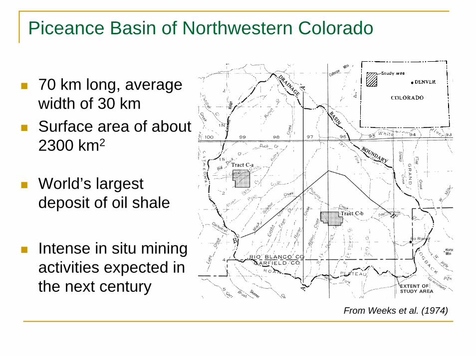
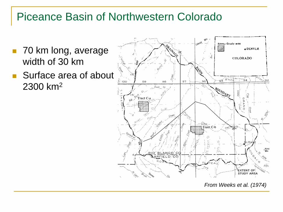
Piceance Basin of Northwestern Colorado
70 km long, average width of 30 kmSurface area of about 2300 km2
World’s largest deposit of oil shale
Intense in situ mining activities expected in the next century
From Weeks et al. (1974)

Potential Environmental Impacts of In Situ Oil Shale Mining
Increase in soil temperatureRelease of large amounts of organic componentsChanges in the chemistry of the soil…

Potential Environmental Impacts of In Situ Oil Shale Mining
Increase in soil temperatureRelease of large amounts of organic componentsChanges in the chemistry of the soil…
Changes in underground conditions will affect groundwater chemistry
Need to understand the fundamental processes involved and develop predictive modelling tools for surface and subsurface water quality

Objectives of this research
Develop an understanding of the effect of local-scale heterogeneities on flow and solute transport at the basin scale
Develop an understanding of the effect of heat distributions on solute transport
Develop efficient modelling approaches to handle coupled heat and solute transport at the basin scale

Outline
Upscaling methods for flow and solute transport
Our approach : FEHM and the GDPM capability
Characterizing heterogeneity in the Piceance basin
Preliminary results : the Mahogany zone
Future work

Upscaling methods for flow and solute transport The need for upscaling methods (1)
Modelling of flow and transport at the
basin scale

Upscaling methods for flow and solute transport The need for upscaling methods (1)
Modelling of flow and transport at the
basin scale
697,323 nodes - 500 x 500 x 25-50 m spacing
7 layers hydrogeologicmodel
From http://meshing.lanl.gov/proj/OIL_SHALE_Piceance/

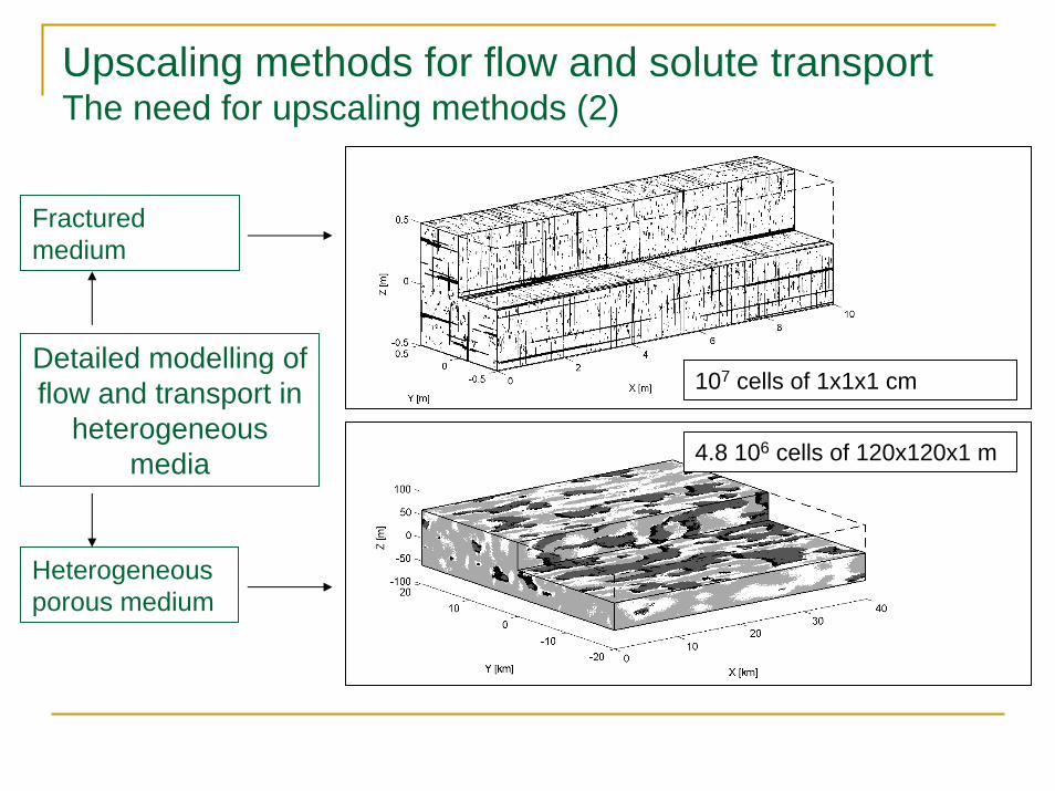
Upscaling methods for flow and solute transport The need for upscaling methods (2)
Detailed modelling of flow and transport in
heterogeneous media

Upscaling methods for flow and solute transport The need for upscaling methods (2)
Detailed modelling of flow and transport in
heterogeneous media
Fracturedmedium
107 cells of 1cm x 1cm x 1cm
Upscaling methods for flow and solute transport The need for upscaling methods (2)
Detailed modelling of flow and transport in
heterogeneous media
107 cells of 1x1x1 cm
4.8 106 cells of 120x120x1 m
Fracturedmedium
Heterogeneous porous medium
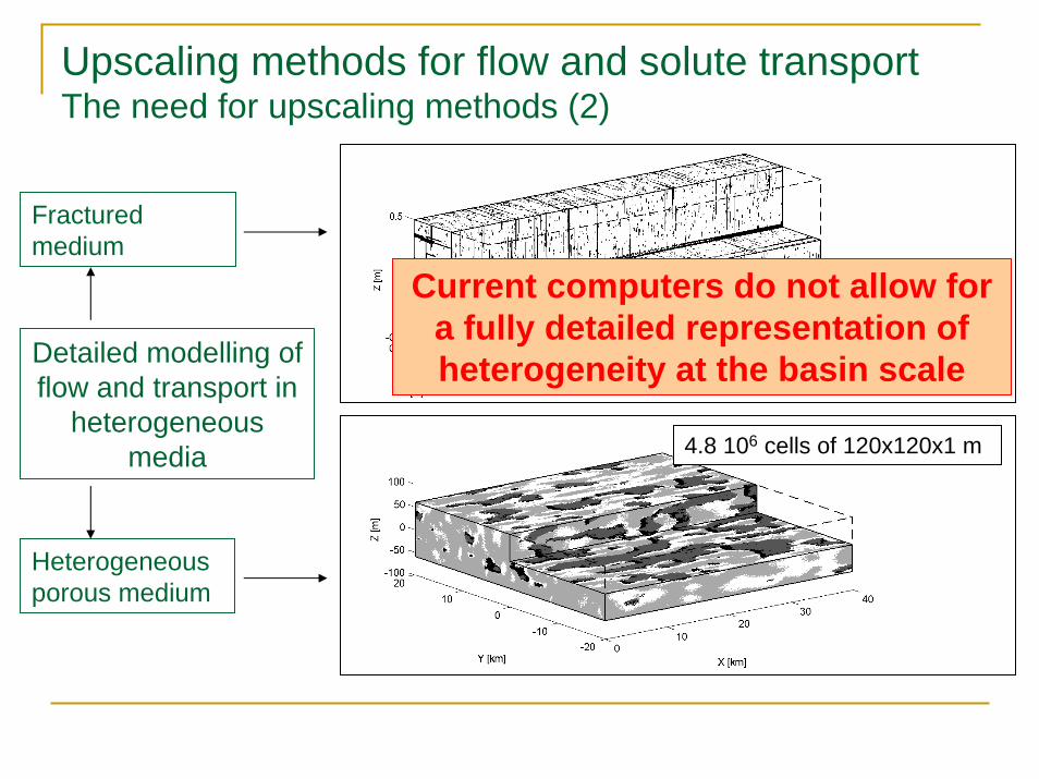
Upscaling methods for flow and solute transport The need for upscaling methods (2)
Detailed modelling of flow and transport in
heterogeneous media
107 cells of 1x1x1 cm
4.8 106 cells of 120x120x1 m
Fracturedmedium
Heterogeneous porous medium
Current computers do not allow for a fully detailed representation of heterogeneity at the basin scale
Anyway, current field characteriz-ation methods do not allow a for fully detailed representation of
heterogeneity at the basin scale

Our approach : FEHM and the GDPM capabilityA finite element heat and mass transport code
Control-volume finite-element formulationMore stable than the traditional FE methodEquivalent to block-centered FD for orthogonal grids
Structured and unstructured gridsCoupled heat and multiphase mass transportReactive solute transport
Advection-dispersion equationDual-porosity formulation : the GDPM capability

Our approach : FEHM and the GDPM capabilityThe generalized dual-porosity model (1)
Dual-porosity solute transport modelClassical dual-porosity models :
Approximate model for transverse diffusive transfer between rock fractures and matrix

Our approach : FEHM and the GDPM capabilityThe generalized dual-porosity model (2)
The generalized dual-porosity model :
Exact model for transverse diffusive transfer between rock fractures and matrix

Our approach : FEHM and the GDPM capabilityThe generalized dual-porosity model (3)
Example : solute transport through a single fracture
Step injection at domain inlet at time t=0
Steady-state saturated flow conditions

Our approach : FEHM and the GDPM capabilityThe generalized dual-porosity model (3)
Example : solute transport through a single fracture
Step injection at domain inlet at time t=0
Steady-state saturated flow conditions

Our approach : FEHM and the GDPM capabilityThe generalized dual-porosity model (3)
Example : solute transport through a single fracture
Full system : 81 sec.
GDPM : 1.5 sec.
Step injection at domain inlet at time t=0
Steady-state saturated flow conditions

Outline
Upscaling methods for flow and solute transportOur approach : FEHM and the GDPM capabilityCharacterizing heterogeneity in the Piceance basin
Markov Chain transition probabilitiesExample : the Uinta Formation2D and 3D realizations of heterogeneous blocks of soil
Preliminary results : the Mahogany zoneFuture work

Characterizing heterogeneity in the Piceance basinMarkov Chain transition probabilities
Finite number of categorical variables (facies)Development of transition probabilities based on core data
Markov Chain model features :Volumetric proportions of faciesMean length of faciesJuxtapositional tendencies
( )ijt h = probability of finding facies j at a distance h of a location where facies i is observed

Characterizing heterogeneity in the Piceance basinExample : the Uinta Formation
Examples of facies transitions based on available core data :
4 facies :1 : siltstone2 : sandstone3 : marlstone4 : oil shale

Characterizing heterogeneity in the Piceance basinExample : the Uinta Formation (2)
Vertical transition probability model :
Legend :o : experimental TP– : Markov Chain model

Characterizing heterogeneity in the Piceance basin2D and 3D realizations of heterogeneous blocks of soil
Uinta Formation
Leached Zone :Model of fracture distribution Nahcolite dissolution

Preliminary results : the Mahogany zoneModel of heterogeneity
Models of fracture distribution resulting from hydraulic fracturing Two-dimensional transition probability model
Volumetric proportion of fractures : 20 %Mean length of horizontal fractures : 5 mMean thickness of horizontal fractures : 2 cmMean length of vertical fractures : 20 cmMean thickness of vertical fractures : 1 cm
Two-dimensional simulations of flow and transport5 m x 1 m blocks1 cm x 1 cm cells (5,000,000 cells)20 realizations

Preliminary results : the Mahogany zoneModel of heterogeneity
Models of fracture distribution resulting from hydraulic fracturing Two-dimensional transition probability model
Two-dimensional simulations of flow and transport5 m x 1 m blocks1 cm x 1 cm cells (5,000,000 cells)20 realizations
Random realization

Preliminary results : the Mahogany zoneModel of heterogeneity
Models of fracture distribution resulting from hydraulic fracturing Two-dimensional transition probability model
Two-dimensional simulations of flow and transport5 m x 1 m blocks1 cm x 1 cm cells (5,000,000 cells)20 real. (flow) and 10 real. (transp.)
Random realization
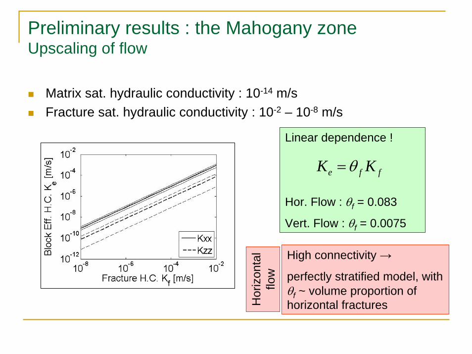
Preliminary results : the Mahogany zone Upscaling of flow
Matrix sat. hydraulic conductivity : 10-14 m/sFracture sat. hydraulic conductivity : 10-2 – 10-8 m/s
Linear dependence !
Hor. Flow : θf = 0.083
Vert. Flow : θf = 0.0075
e f fK Kθ=
High connectivity →
perfectly stratified model, with θf ~ volume proportion of horizontal fracturesH
oriz
onta
l flo
w
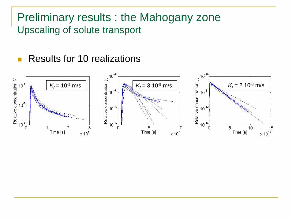
Preliminary results : the Mahogany zone Upscaling of solute transport
Results for 10 realizations
Kf = 10-2 m/s Kf = 3 10-5 m/s Kf = 2 10-8 m/s

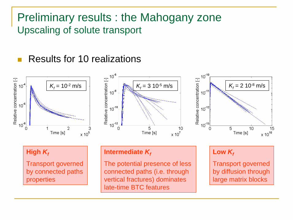
Preliminary results : the Mahogany zone Upscaling of solute transport
Results for 10 realizations
Kf = 10-2 m/s Kf = 3 10-5 m/s Kf = 2 10-8 m/s
High Kf
Transport governed by connected paths properties

Preliminary results : the Mahogany zone Upscaling of solute transport
Results for 10 realizations
Kf = 10-2 m/s Kf = 3 10-5 m/s Kf = 2 10-8 m/s
High Kf
Transport governed by connected paths properties
Intermediate Kf
The potential presence of less connected paths (i.e. through vertical fractures) dominates late-time BTC features
Preliminary results : the Mahogany zone Upscaling of solute transport
Results for 10 realizations
Kf = 10-2 m/s Kf = 3 10-5 m/s Kf = 2 10-8 m/s
High Kf
Transport governed by connected paths properties
Low Kf
Transport governed by diffusion through large matrix blocks
Intermediate Kf
The potential presence of less connected paths (i.e. through vertical fractures) dominates late-time BTC features

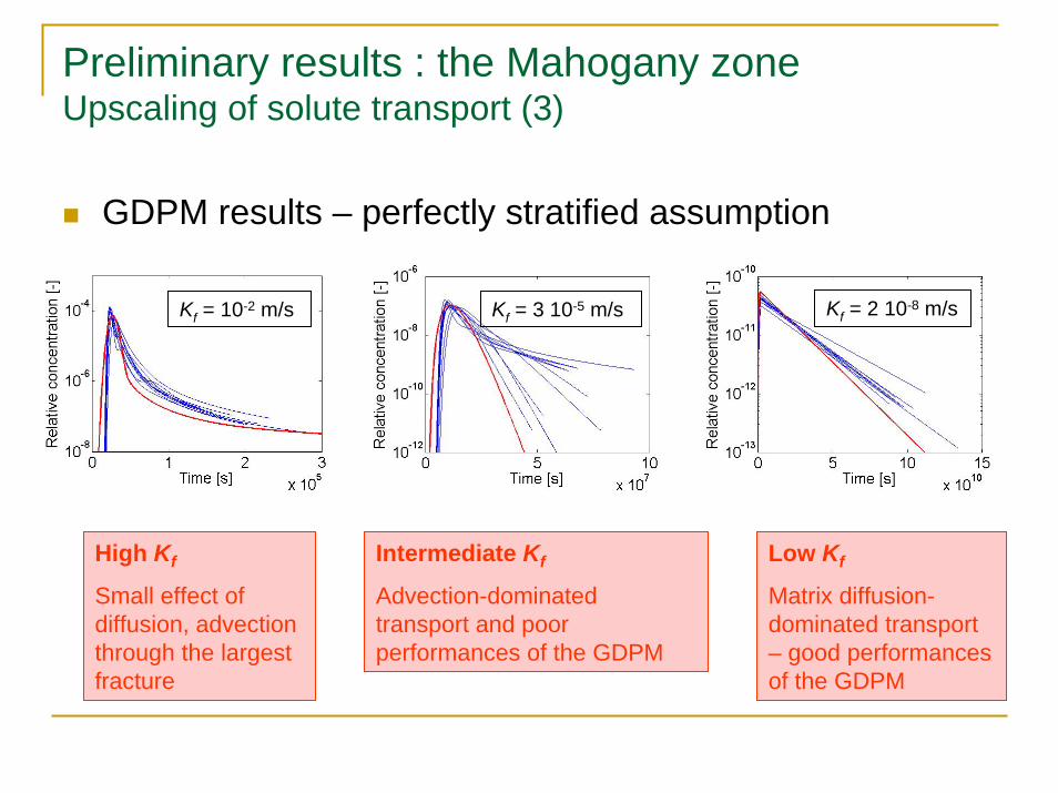
Preliminary results : the Mahogany zone Upscaling of solute transport (3)
GDPM results – perfectly stratified assumption
Kf = 10-2 m/s
High Kf
Small effect of diffusion, advection through the largest fracture

Preliminary results : the Mahogany zone Upscaling of solute transport (3)
GDPM results – perfectly stratified assumption
Kf = 10-2 m/s Kf = 3 10-5 m/s
High Kf
Small effect of diffusion, advection through the largest fracture
Intermediate Kf
Advection-dominated transport and poor performances of the GDPM
Preliminary results : the Mahogany zone Upscaling of solute transport (3)
GDPM results – perfectly stratified assumption
Kf = 10-2 m/s Kf = 3 10-5 m/s Kf = 2 10-8 m/s
High Kf
Small effect of diffusion, advection through the largest fracture
Low Kf
Matrix diffusion-dominated transport – good performances of the GDPM
Intermediate Kf
Advection-dominated transport and poor performances of the GDPM

Future work
Determination of effective GDPM parametersSensitivity analysis for flow and transport
In fractured mediaVolumetric proportion of fracturesMean length of fractures vs block sizeHydraulic conductivity of fracturesDimensionality (2D vs 3D simulations)
In heterogeneous porous mediaHorizontal TP modelFacies hydraulic conductivity
Heat transportCoupled heat and solute transport

Thank you for your attention !
Any questions or comments ?