Multi-objective and Risk-based Modelling Methodology for
Planning, Design and Operation of Water Supply Systems
Von der Fakultat Bau- und Umweltingenieurwissenschaften der Universitat Stuttgart
zur Erlangung der Wurde eines Doktors der
Ingenieurwissenschaften (Dr.-Ing.) genehmigte Abhandlung
Vorgelegt von
Aleksandar Trifkovic
aus Bosnien und Herzegowina
Hauptberichter: Prof. Dr.-Ing. Ulrich Rott
Mitberichter: Prof. Dr. rer. nat. Dr.-Ing. habil. Andras Bardossy
Tag der mundlichen Prufung: 3. Juli 2007
Institut fur Wasserbau der Universitat Stuttgart
2007

Heft 163 Multi-objective and Risk-based
Modelling Methodology for
Planning, Design and
Operation of Water Supply
Systems
von
Dr.-Ing.
Aleksandar Trifkovic
Eigenverlag des Instituts fur Wasserbau der Universitat Stuttgart
D93 Multi-objective and Risk-based Modelling Methodology forPlanning, Design and Operation of Water Supply Systems
Trifkovic, Aleksandar:
Multi-objective and Risk-based Modelling Methodology for Planning, Design and Operation of
Water Supply Systems / von Aleksandar Trifkovic. Institut fur Wasserbau, Universitat Stuttgart. -
Stuttgart: Inst. fur Wasserbau, 2007
(Mitteilungen / Institut fur Wasserbau, Universitat Stuttgart ; H. 163)
Zugl.: Stuttgart, Univ., Diss., 2007
ISBN 3-933761-67-0
Gegen Vervielfaltigung und Ubersetzung bestehen keine Einwande, es wird lediglichum Quellenangabe gebeten.
Herausgegeben 2007 vom Eigenverlag des Instituts fur WasserbauDruck: Sprint-Druck, Stuttgart

Acknowledgement
I would like to express my profound gratitude to Prof. Dr.-Ing. Ulrich Rott and Prof. Dr.
rer. nat. Dr.-Ing. habil. Andras Bardossy for supervising this thesis. Both their guidance
and contribution over the course of writing this thesis have been truly invaluable.
I would also like to thank Dr. rer.nat. Roland Barthel and Jurgen Braun, Ph.D. for their en-
couragement and support during my work and stay at the Institute of Hydraulic Engineering
as a memeber of the Young scientist workgroup Groundwater Hydraulics and Groundwater
Management, and as a member of the GLOWA-Danube project.
As well, I would like to thank my colleagues and members of the workgroup Johanna Jagelke,
Darla Nickel, Dr.-Ing. Vlad Rojanschi, Dr.-Ing. Jens Wolf and Dr.-Ing. Jens Modringer for
numerous thoughtful discussions, useful suggestions and sharing of experience over the course
of the model development. They as well as Marco Borchers and Jan van Heyden, WAREM
staff Claudia Hojak and Yvonne Reichert and colleagues from the Institute of Hydraulic
Engineering like Sandra Prohaska, Milos Vasin and Alexandros Papafotiou have made my
time in Stuttgart such a wonderful experience.
Finally, I would like to thank my wife Irena and our daughter Ana for all of their love and
encouragement. I thank our parents and my sister for sincere trust and above all my father
who has always been my greatest inspiration and ideal.
Financial support for this study was provided by the Federal Ministry of Education and
Research of Germany through the International Postgraduate Studies in Water Technologies
(IPSWaT) program. The persons who managed the program within my participation in the
International Doctoral Program Environment Water (ENWAT) Dr.-Ing. Sabine Manthey,
Andrea Bange and Rainer Enzenhoefer are also gratefully acknowledged.

Contents
Acknowledgement V
List of Figures V
List of Tables IX
List of Abbreviations X
Notation XI
Abstract XV
Zusammenfassung XVII
1. Introduction 1
1.1. Motivation . . . . . . . . . . . . . . . . . . . . . . . . . . . . . . . . . . . . . 1
1.2. General Objectives and Current Problems of Interests . . . . . . . . . . . . . 4
1.3. Specific Objectives and the Aim of the Research . . . . . . . . . . . . . . . . 6
1.4. Course of Action . . . . . . . . . . . . . . . . . . . . . . . . . . . . . . . . . . 7
2. Foundations of the Study 9
2.1. Main Characteristics of Water Supply Systems . . . . . . . . . . . . . . . . . 9
2.1.1. Physical Characteristics . . . . . . . . . . . . . . . . . . . . . . . . . . 9
2.1.2. Water Supply . . . . . . . . . . . . . . . . . . . . . . . . . . . . . . . . 11
2.1.3. Water Demand . . . . . . . . . . . . . . . . . . . . . . . . . . . . . . . 11
2.1.4. System Performance Measures . . . . . . . . . . . . . . . . . . . . . . 12
2.2. Environmental and Socioeconomic Issues of Importance . . . . . . . . . . . . 12
2.2.1. Environmental Impacts of Water Supply Systems . . . . . . . . . . . . 12
2.2.2. Quantification of Environmental Costs and Benefits . . . . . . . . . . 13
2.2.3. Socioeconomic Aspects of Water Supply Systems . . . . . . . . . . . . 15
2.2.4. Quantification of Socioeconomic Costs and Benefits . . . . . . . . . . 16
2.3. Uncertainty, Risk and Reliability in Water Supply Systems . . . . . . . . . . 17
2.4. Management and Analysis of Water Supply Systems . . . . . . . . . . . . . . 20
2.4.1. System Analysis in Planning of Water Supply Systems . . . . . . . . . 21
2.4.2. System Analysis in Design of Water Supply Systems . . . . . . . . . . 24
2.4.3. System Analysis in Operation of Water Supply Systems . . . . . . . . 29
II Contents
3. Methodology Development 32
3.1. Representation of Water Supply Systems and Objectives of the Analysis . . . 32
3.1.1. Water Supply System’s Structure . . . . . . . . . . . . . . . . . . . . . 32
3.1.2. Water Supply System’s Function . . . . . . . . . . . . . . . . . . . . . 35
3.1.3. Formulation of the Optimization Problem . . . . . . . . . . . . . . . . 38
3.2. Method for the Integration of Environmental and Socioeconomic Aspects . . 39
3.2.1. Representation of Water Supply System’s Impacts . . . . . . . . . . . 40
3.2.2. Scaling of Impact Functions . . . . . . . . . . . . . . . . . . . . . . . . 42
3.2.3. Multiple Criteria Analysis of Impact Functions . . . . . . . . . . . . . 43
3.2.4. Integrative Analysis of Fixed and Variable Impacts . . . . . . . . . . . 46
3.3. Methods for the Solution of the Optimisation Problem . . . . . . . . . . . . . 49
3.3.1. Characteristics of the Optimisation Problem . . . . . . . . . . . . . . 49
3.3.2. Initial Solution with the Maximum Feasible Flow Method . . . . . . . 51
3.3.3. Primal Solution with the Simulated Annealing Method . . . . . . . . . 53
3.3.4. Adaptation of the Simulated Annealing for Multi-objective Problem . 55
3.3.5. Final Solution with the Branch and Bound Method . . . . . . . . . . . 58
3.4. Method for the Integration of Uncertainty, Risk and Reliability Considerations 60
3.4.1. Component Failure Analysis with the Path Restoration Method . . . . 61
3.4.2. Performance Failure Analysis with the Latin Hypercube Sampling
Method . . . . . . . . . . . . . . . . . . . . . . . . . . . . . . . . . . . 63
3.4.3. System Performance Calculation and Risk-Oriented Selection of Alter-
natives . . . . . . . . . . . . . . . . . . . . . . . . . . . . . . . . . . . . 65
4. Model Development and Application 67
4.1. Planning Model . . . . . . . . . . . . . . . . . . . . . . . . . . . . . . . . . . . 67
4.1.1. Characterisation of the Planning Problem . . . . . . . . . . . . . . . . 67
4.1.2. Accommodation of the Solution Methodology . . . . . . . . . . . . . . 69
4.1.3. Case Study P1 - Planning Model Demonstration . . . . . . . . . . . . 72
4.1.4. Case Study P2 - Planning Model Validation . . . . . . . . . . . . . . . 82
4.2. Design Model . . . . . . . . . . . . . . . . . . . . . . . . . . . . . . . . . . . . 91
4.2.1. Characterisation of the Design Problem . . . . . . . . . . . . . . . . . 91
4.2.2. Accommodation of the Solution Methodology . . . . . . . . . . . . . . 94
4.2.3. Case Study D1 - Design Model Demonstration . . . . . . . . . . . . . 97
4.2.4. Case Study D2 - Design Model Validation . . . . . . . . . . . . . . . . 106
4.3. Operation Model . . . . . . . . . . . . . . . . . . . . . . . . . . . . . . . . . . 113
4.3.1. Characterisation of the Operation Problem . . . . . . . . . . . . . . . 113
4.3.2. Accommodation of the Solution Methodology . . . . . . . . . . . . . . 115
4.3.3. Case Study O1 - Operation Model Demonstration . . . . . . . . . . . 117
4.3.4. Case Study O2 - Operation Model Validation . . . . . . . . . . . . . . 124
5. Conclusions and Outlook 132
5.1. Methodology Development . . . . . . . . . . . . . . . . . . . . . . . . . . . . . 132
5.2. Models Development . . . . . . . . . . . . . . . . . . . . . . . . . . . . . . . . 134
5.3. Outlook . . . . . . . . . . . . . . . . . . . . . . . . . . . . . . . . . . . . . . . 136

Contents III
A. Appendix II
A.1. Environmental Impacts of Water Supply Projects . . . . . . . . . . . . . . . . II


List of Figures
0.1. Hierarchischen Ansatz zu Wasserversorgungsmanagement (Jamieson, 1981) . XVIII
0.2. Fallstudie P1: Netzkonfiguration [Adaptation von Alperovits and Shamir (1977)]XIX
0.3. Fallstudie P1: Berechnete individuelle Losungen . . . . . . . . . . . . . . . . XX
0.4. Fallstudie P1: Berechnete Werte der okonomischen, okologischen und sozialen
Kriterien fur die Mehrziel-Losungen . . . . . . . . . . . . . . . . . . . . . . . XXI
0.5. Fallstudie D1: Berechnete optimale Erweiterung von Leitungsdurchmessern
fur Ausfalle der Komponenten A8, A9, A10, A11 . . . . . . . . . . . . . . . . XXIII
0.6. Fallstudie D1: Statistische Auswertung von berechneten Drucke fur Stichprobe
ohne und mit Bedarfsbeziehung . . . . . . . . . . . . . . . . . . . . . . . . . . XXIV
0.7. Fallstudie O1: Identifizierte optimale Pumpensteuerung und entsprechende
Behalterwasserniveau fur Behalterkapazitat von 50 m2 . . . . . . . . . . . . . XXV
0.8. Fallstudie O1: Identifizierte optimale Pumpensteuerung und entsprechende
Behalterwasserniveau fur Behalterkapazitat von 55 m2 . . . . . . . . . . . . . XXVI
1.1. Relative growth of world population, gross world product, industrial sector,
irrigated area and water demand [source: Hoekstra, 1998] . . . . . . . . . . . 1
1.2. Integrative approach to the analysis of infrastructural systems [adopted from
UN, 1992] . . . . . . . . . . . . . . . . . . . . . . . . . . . . . . . . . . . . . . 2
1.3. Decision support in management of water supply system [adopted from Loucks
and da Costa, 1991] . . . . . . . . . . . . . . . . . . . . . . . . . . . . . . . . 3
2.1. Components of water supply systems [source: Grigg, 1986] . . . . . . . . . . . 10
2.2. Branched, semi-looped and looped layout . . . . . . . . . . . . . . . . . . . . 10
2.3. Shematised cost-reliability [source: Shamir, 2002] and risk-reliability curves . 17
2.4. Traditional and stochastic [source: Plate, 2000] design approaches . . . . . . 19
2.5. Hierarchical approach to the management of water supply systems (Jamieson,
1981) . . . . . . . . . . . . . . . . . . . . . . . . . . . . . . . . . . . . . . . . . 21
3.1. Network representation of water supply systems . . . . . . . . . . . . . . . . . 34
3.2. Adopted typical forms of cost (negative impact) functions . . . . . . . . . . . 41
3.3. Transformation of a function to the unit-function . . . . . . . . . . . . . . . . 42
3.4. Multi criteria analysis of water supply systems [source: Munasinghe, 1997] . . 44
3.5. Pareto-optimal set, [source: Liu et al., 2001] . . . . . . . . . . . . . . . . . . . 45
3.6. Integration of fixed and variable costs (impacts) . . . . . . . . . . . . . . . . . 46
3.7. Linear approximation of convex and concave functions . . . . . . . . . . . . . 50
3.8. Main steps of the optimisation procedure . . . . . . . . . . . . . . . . . . . . 51
3.9. Acceptance problem in multi-criteria optimization [source Ulungu et al., 1999] 56
VI List of Figures
4.1. Flow chart of the planning model . . . . . . . . . . . . . . . . . . . . . . . . . 71
4.2. Case study P1: Network configuration [adaptation from Alperovits and Shamir
(1977)] . . . . . . . . . . . . . . . . . . . . . . . . . . . . . . . . . . . . . . . . 72
4.3. Case study P1: Input economic, environmental and social cost (impact) func-
tions [fictitious] . . . . . . . . . . . . . . . . . . . . . . . . . . . . . . . . . . . 74
4.4. Case study P1: Identified initial solution . . . . . . . . . . . . . . . . . . . . . 76
4.5. Case study P1: Identified primal solution . . . . . . . . . . . . . . . . . . . . 77
4.6. Case study P1: Obtained values on economic, environmental and social criteria
during identification of the primal solution . . . . . . . . . . . . . . . . . . . . 78
4.7. Case study P1: Identified single-objective solutions (economical, environmen-
tal and social) and their improvements relative to the primal solution . . . . 79
4.8. Case study P1: Comparison of the multi-objective solutions with the primal
one for different weight combinations . . . . . . . . . . . . . . . . . . . . . . . 81
4.9. Case study P1: Obtained values on economic, environmental and social criteria
(relative to the primal solution) during identification of the multi-objective
solutions . . . . . . . . . . . . . . . . . . . . . . . . . . . . . . . . . . . . . . . 82
4.10. Case study P2: Network configuration [adaptation from Vink and Schot (2002)] 83
4.11. Case Study P2: Input vegetation damage and purification cost functions [Vink
and Schot (2002)] . . . . . . . . . . . . . . . . . . . . . . . . . . . . . . . . . . 85
4.12. Case study P2: Obtained values on economic, environmental and social criteria
during identification of the primal solution . . . . . . . . . . . . . . . . . . . . 86
4.13. Case study P2: Comparison of the multi-objective solutions to the primal one
for different weight combinations . . . . . . . . . . . . . . . . . . . . . . . . . 87
4.14. Case study P2: Obtained values on economic, environmental and social criteria
(relative to the primal solution) during identification of the multi-objective
solutions . . . . . . . . . . . . . . . . . . . . . . . . . . . . . . . . . . . . . . . 88
4.15. Case Study P2: Progress of the optimisation for the case studies P1 and P2 89
4.16. Case Study P2: Progress of the optimisation on individual criteria for the case
studies P1 and P2 . . . . . . . . . . . . . . . . . . . . . . . . . . . . . . . . . 89
4.17. Case Study P2: Progress of the optimisation for the case study P2 with 10
and 48 wells . . . . . . . . . . . . . . . . . . . . . . . . . . . . . . . . . . . . . 90
4.18. Decomposition applied in the design model . . . . . . . . . . . . . . . . . . . 93
4.19. Flow chart of the design model . . . . . . . . . . . . . . . . . . . . . . . . . . 96
4.20. Case study D1: Network configuration of the selected planning solution . . . 98
4.21. Case Study D1: Identified primal solution . . . . . . . . . . . . . . . . . . . . 99
4.22. Case study D1: Increase of the network capacities for selected component
failure scenarios . . . . . . . . . . . . . . . . . . . . . . . . . . . . . . . . . . . 101
4.23. Case study D1: Relative increase in investment costs for selected component
failure scenarios . . . . . . . . . . . . . . . . . . . . . . . . . . . . . . . . . . . 102
4.24. Case study D1: Independent and uniform water demand samples with 15 %
and 30 % uncertainty tresholds . . . . . . . . . . . . . . . . . . . . . . . . . . 103
4.25. Case study D1: Statistic of the water demand samples with 15 % and 30 %
uncertainty tresholds . . . . . . . . . . . . . . . . . . . . . . . . . . . . . . . . 103
4.26. Case study D1: Obtained flows in arcs for demand samples with 15 % and
30 % uncertainty tresholds . . . . . . . . . . . . . . . . . . . . . . . . . . . . . 104
List of Figures VII
4.27. Case study D1: Obtained pressures at nodes for demand samples with 15 %
and 30 % uncertainty tresholds . . . . . . . . . . . . . . . . . . . . . . . . . . 104
4.28. Case study D1: Statistics of the calculated arc flows . . . . . . . . . . . . . . 105
4.29. Case study D1: Statistics of the calculated nodal pressures . . . . . . . . . . 105
4.30. Case study D1: Correlated and uniform water demand samples with 30 %
unceratinty threshold and corresponding calculated nodal pressure statistics . 106
4.31. Case study D2a: Network configuration of the 2-loop network [Alperovits and
Shamir (1977)] . . . . . . . . . . . . . . . . . . . . . . . . . . . . . . . . . . . 107
4.32. Case study D2b: Network configuration of the 3-loop network [Fujiwara and
Khang (1990)] . . . . . . . . . . . . . . . . . . . . . . . . . . . . . . . . . . . . 108
4.33. Case study D2b: Relative total cost reduction for the relaxation of the mini-
mum pressure constraint . . . . . . . . . . . . . . . . . . . . . . . . . . . . . . 111
4.34. Case study D2a and D2b: Progress of the optimisation for the 2-loop and
3-loop network’s optimisation . . . . . . . . . . . . . . . . . . . . . . . . . . . 112
4.35. Integration of Network Solver in the operation optimisation model . . . . . . 115
4.36. Flow chart of the operation model . . . . . . . . . . . . . . . . . . . . . . . . 117
4.37. Case study O1: Network Configuration [adapted Alperovits and Shamir (1977)]118
4.38. Case study O1: Adopted water demand coefficient [as in Walski et al. (1987)]
and energy cost coefficient [typical 3-phase partitioning] . . . . . . . . . . . . 118
4.39. Case study O1: Obtained pump operation schedule and tank water level for
the primal solution [tank area of 50 m2] . . . . . . . . . . . . . . . . . . . . . 121
4.40. Case study O1: Identified tank investment and pump operation costs values
during single-objective optimisation . . . . . . . . . . . . . . . . . . . . . . . 121
4.41. Case study O1: Obtained pump operation schedule and tank water level for
the final solution [tank area of 55 m2] . . . . . . . . . . . . . . . . . . . . . . 122
4.42. Case study O1: Identified tank investment and pump operation costs values
during multi-objective optimisation . . . . . . . . . . . . . . . . . . . . . . . . 123
4.43. Case study O1: Obtained minimum pressures for the primal and the final
solution . . . . . . . . . . . . . . . . . . . . . . . . . . . . . . . . . . . . . . . 124
4.44. Case study O2: Network configuration [adaptation from Walski et al. (1987)] 125
4.45. Case study O2: Obtained pump operation schedule and tank water levels for
the primal solution . . . . . . . . . . . . . . . . . . . . . . . . . . . . . . . . . 127
4.46. Case study O2: Identified final solution . . . . . . . . . . . . . . . . . . . . . 128
4.47. Case study O2: Obtained pump operation schedule and tank water level for
the final solution . . . . . . . . . . . . . . . . . . . . . . . . . . . . . . . . . . 129
4.48. Case study O1: Progress of the optimisation for random and weighted neigh-
bourhood function . . . . . . . . . . . . . . . . . . . . . . . . . . . . . . . . . 130
4.49. Case study O2: Progress of the optimisation for the final solution . . . . . . . 131

List of Tables
0.2. Fallstudie D1: Berechnete optimale Durchflusse, Druck und Druckverluste . . XXII
4.1. Case study P1: Characteristics of the network [adaptation from Alperovits
and Shamir (1977)] . . . . . . . . . . . . . . . . . . . . . . . . . . . . . . . . . 73
4.2. Case study P2: Characteristics of the network (adaptation from Vink and
Schot (2002)) . . . . . . . . . . . . . . . . . . . . . . . . . . . . . . . . . . . . 84
4.3. Case study P2: Identified initial, primal and single-objective solutions . . . . 85
4.4. Case StudyD1: Standard set of available pipe diameters with their investment
costs per unit length [source: Alperovits and Shamir (1977)] . . . . . . . . . . 98
4.5. Case study D1: Calculated flow, head loss and pressures for the primal solution100
4.6. Case study D2b: Characteristics of the 3-loop network (adaptation from Fuji-
wara and Khang (1990)) . . . . . . . . . . . . . . . . . . . . . . . . . . . . . . 107
4.7. Case study D2b: Additional pipe diameters with their investment costs per
unit length [source: Fujiwara and Khang (1990)] . . . . . . . . . . . . . . . . 108
4.8. Case study D2a: Comparison of the obtained solution with in literature re-
ported solutions for the 2-loop network . . . . . . . . . . . . . . . . . . . . . . 109
4.9. Case study D2b: Comparison of the obtained solution with in literature re-
ported solutions for the 3-loop network . . . . . . . . . . . . . . . . . . . . . . 110
4.10. Case study O2: Characteristics of network arcs [adaptation of Walski et al.
(1987)] . . . . . . . . . . . . . . . . . . . . . . . . . . . . . . . . . . . . . . . . 126
4.11. Case studyO2: Characteristics of network nodes [adaptation fromWalski et al.
(1987)] . . . . . . . . . . . . . . . . . . . . . . . . . . . . . . . . . . . . . . . . 126
A.1. Impacts of water supply systems on air quality [source: CIRIA, 1994] . . . . II
A.2. Impacts of water supply systems on water quantity and quality [source: CIRIA,
1994] . . . . . . . . . . . . . . . . . . . . . . . . . . . . . . . . . . . . . . . . . II
A.3. Impacts of water supply systems on land [source: CIRIA, 1994] . . . . . . . . II
A.4. Impacts of water supply systems on natural habitats [source: CIRIA, 1994] . III

List of Abbreviations
Abbreviation Denotation
a annual
DSS Decision Support System
EIA Environmental Impact Assessment
EPANET Simulation program for pressurized networks
FORTRAN Formula Translator (Programming language)
ft feet (1 ft = 0.3048 m)
GIS Geographic Information System
gpm gallon per minute (1 gpm = 0.000067 m3/s)
hr hour
ILHS Improved Latin Hypercube Sampling
in inch (1 in = 0.0254 m)
LHS Latin Hypercube Sampling
m meter
m.a.s.l meter above sea level
MCDA Multiple Criteria Decision Analysis
MCDM Multiple Criteria Decision Making
MOSA Multi-objective Simulated Annealing
nmb number
yEd JavaTM Graph Editor for visualisation of graphs
Notation
Symbol Definition Dimension
G graph [ - ]
ni node (vertix) i [ - ]
N set of nodes [ - ]
aij arc (edge) from node ni to node nj [ - ]
A set of arcs [ - ]
d(ni) degree of a node ni [ number ]
do(ni) outdegree of a node ni [ number ]
di(ni) indegree of a node ni [ number ]
π path [ - ]
π+ forward path [ - ]
π− backward path [ - ]
Gn network [ - ]
S arbitrary set [ - ]
Q set of rational numbers [ - ]
R+0 set of positive rational numbers with zero [ - ]
κij upper capacity of arc aij [ m3/s ]
λij lower capacity of arc aij [ m3/s ]
xij flow of water in arc aij [ m3/s ]
x flow vector (flow pattern) on a network Gn [ m3/s ]
xπ flow on path π (path flow) [ m3/s ]
Lij length of pipe aij [ m ]
Aij cross section area of pipe aij [ m2 ]
Cτij friction coefficient of pipe aij [ number ]
rij pipe characteristics of aij [ number ]
zi elevation of node ni [ m ]
pi hydrostatic pressure at node ni [ Pa ]
Πi pressure head at node ni [ m ]
bi external flow at node ni [ m3/s ]
Smaxi maximum available supply at node ni [ m3/s ]
Dmini minimum needed demand at node ni [ m3/s ]
λij Darcy-Weissbach friction coefficient of pipe aij [ number ]
Cij Hazen-Williams friction coefficient of pipe aij [ number ]
XII Notation
nij Chezy-Manning friction coefficient of pipe aij [ number ]
k unit conversion factor bertween English and SI units [ number ]
z total costs of the network (flow transport) problem [ value ]
cij cost coefficient of arc aij [ value/[x]]
πk conforming simple path [ - ]
xπk flow on conforming path πk [ m3/s ]
c(x) cost function of some system parameter x [ value/[x] ]
q, p, r parameters of some cost function c(x) [ number ]
s(c) scaling function of some cost function c(x) [ value ]
C(x) unit cost function of some cost function c(x) [ number ]
C l(x) total impact function of some system parameter x [ number ]
Cecn(x) economic impact function of some system parameter x [ number ]
Cenv(x) environmental impact function of some system parameter x [ number ]
Csoc(x) socio impact function of some system parameter x [ number ]
Csyst(x) system quality impact function of some system parameter x [ number ]
zi solution of the network flow problem on objective i [ value ]
ziw solution of the network flow problem on objective i for combi-
nation of weights toward different objectives w
[ value ]
Cfixijfixed impact function for some system element aij [ number ]
Cvarij variable impact function for some system element aij [ number ]
PV present value of some investment [ value ]
FV future value of some investment [ value ]
A annuity for some system costs or benefits in some compounding
period
[ value ]
at weights toward different annuity values [ value ]
PV A present value to annuity of some investment [ value ]
FV A future value to annuity of some investment [ value ]
DPV discounted present value of some investment [ value ]
r interest rate [ % ]
t time period [ years ]
n length of time period [ years ]
DCvar discounted variable impacts to the present value [ value ]
yij integer variable to distinguisch existing and potential elements
aij
[ number ]
O set of origin nodes [ - ]
T set of terminal nodes [ - ]
AO,T cut in a network Gn with sets O and T [ - ]
κO,T cut in a network Gn with sets O and T [ - ]
πa augmenting path [ - ]
xπa flow on augmenting path πk [ m3/s ]
X set of flow vectors on a network Gn [ m3/s ]
Z set of function values (solutions) for a set of flow vectors X [ value ]
T temperature at some energy level in Simulated Annealing [ number ]
Tmax initial temperature in Simulated Annealing [ number ]
Tmin minimal temperature in Simulated Annealing [ number ]
Notation XIII
ΔT temperature decrease parameter in Simulated Annealing [ number ]
Nmax maximal number of changes at some energy level in Simulated
Annealing
[ number ]
Nsucc maximal number of successful changes at some energy level in
Simulated Annealing
[ number ]
B constant that relates temperature to the function value in Sim-
ulated Annealing
[ number ]
Δx random flow change in Simulated Annealing [ m3/s ]
Δz change of the function value (solution) in Simulated Annealing [ value ]
ΔP penalty constant for the consideration of pressure constraints [ value ]
W l combination of weights toward different function criteria l [ number ]
Ω set of combination of weights W l [ number ]
ΩD set of dominant combination of weights W l [ number ]
Δzl change of the function value on criteria l in MOSA [ value ]
Δzw weighted change of the function value for all criteria in MOSA [ value ]
Δs aggregate function change in MOSA [ number ]
O() time complexity function [ number ]
z lower bound solution in Branch and Bound [ value ]
z upper bound solution in Branch and Bound [ value ]
s failure scenario in Path Restoration Method [ - ]
f failure source-destination paths for scenario s [ - ]
F set of all failure source-destination paths for failure scenario s [ - ]
Qsf total affected flow on failed path f for failure scenario s [ m3/s ]
r restoration source-destination paths for failed path f [ - ]
R set of all restoration source-destination paths for failed path f [ - ]
xπf,rs flow on restoration path r for the failed path f in failure scenario
s
[ m3/s ]
Hs(xπf,r
s) head at source node of the path xπf,rs [ m ]
Hd(xπf,r
s) head at destination node of the path xπf,rs [ m ]
ΔH(δsf,rixπf,r
s) sum of all losses on the path xπf,rs [ m ]
Di variable i in sampling technique ILHS [ - ]
N number of variables to sample with ILHS [ number ]
j interval of the sampling in ILHS [ - ]
M number of sampling intervals in ILHS [ number ]
P (Dji ) probability density function of the interval j in variable i [ number ]

XIV Notation
Subscripts:
i node
s supply node
d demand node
t transshipment node
S slack node
ij arc
k conforming
a augmenting
w weighted
fix fixed
var variable
min minimum
max maximum
Superscripts:
π path
l objective, criteria′ iteration′′ next iteration
˙ temperature level
¨ next temperature level
D dominant solutions
s failure scenario
t time
env environmental
ecn economic
soc socio
syst system quality
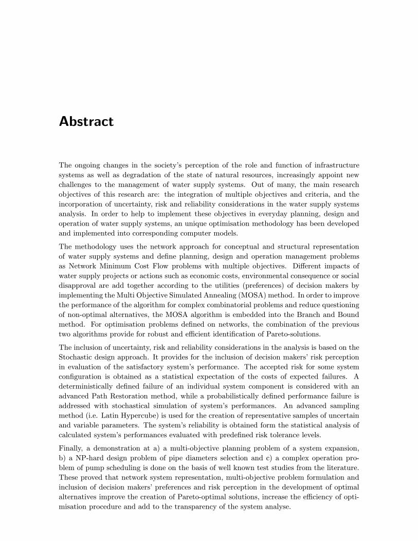
Abstract
The ongoing changes in the society’s perception of the role and function of infrastructure
systems as well as degradation of the state of natural resources, increasingly appoint new
challenges to the management of water supply systems. Out of many, the main research
objectives of this research are: the integration of multiple objectives and criteria, and the
incorporation of uncertainty, risk and reliability considerations in the water supply systems
analysis. In order to help to implement these objectives in everyday planning, design and
operation of water supply systems, an unique optimisation methodology has been developed
and implemented into corresponding computer models.
The methodology uses the network approach for conceptual and structural representation
of water supply systems and define planning, design and operation management problems
as Network Minimum Cost Flow problems with multiple objectives. Different impacts of
water supply projects or actions such as economic costs, environmental consequence or social
disapproval are add together according to the utilities (preferences) of decision makers by
implementing the Multi Objective Simulated Annealing (MOSA) method. In order to improve
the performance of the algorithm for complex combinatorial problems and reduce questioning
of non-optimal alternatives, the MOSA algorithm is embedded into the Branch and Bound
method. For optimisation problems defined on networks, the combination of the previous
two algorithms provide for robust and efficient identification of Pareto-solutions.
The inclusion of uncertainty, risk and reliability considerations in the analysis is based on the
Stochastic design approach. It provides for the inclusion of decision makers’ risk perception
in evaluation of the satisfactory system’s performance. The accepted risk for some system
configuration is obtained as a statistical expectation of the costs of expected failures. A
deterministically defined failure of an individual system component is considered with an
advanced Path Restoration method, while a probabilistically defined performance failure is
addressed with stochastical simulation of system’s performances. An advanced sampling
method (i.e. Latin Hypercube) is used for the creation of representative samples of uncertain
and variable parameters. The system’s reliability is obtained form the statistical analysis of
calculated system’s performances evaluated with predefined risk tolerance levels.
Finally, a demonstration at a) a multi-objective planning problem of a system expansion,
b) a NP-hard design problem of pipe diameters selection and c) a complex operation pro-
blem of pump scheduling is done on the basis of well known test studies from the literature.
These proved that network system representation, multi-objective problem formulation and
inclusion of decision makers’ preferences and risk perception in the development of optimal
alternatives improve the creation of Pareto-optimal solutions, increase the efficiency of opti-
misation procedure and add to the transparency of the system analyse.


Zusammenfassung
Motivation und Zielsetzung
Die verstarkte Nutzung der naturlichen Wasserressourcen und die weltweite Verunreinigung
dieses kostbaren Schatzes im 20. Jahrhundert fuhrte zur Erschopfung und Verschmutzung
vieler naturlicher Wasserkorper und zur Zerstorung zahlreicher Okosysteme. Die wachsende
Spannung zwischen intensiver Wassernutzung und der naturlichen Funktion von Okosyste-
men, veranderte unsere Vorstellung uber die Aufgabe der Wasserversorgungssysteme von den
human utility services hin zu den coupled human-natural systems (Allenby, 2004). Die integra-
tive Betrachtung von Umwelt und kunstlichen Systemen, stellt ein neues Paradigma unserer
Gesellschaft dar (IUCN et al., 1980; UN, 1992). Allerdings stehlt die integrierte Betrachtung
von gesellschaftlicher, okonomischer und okologischer Aspekte von Wasserversorgungssyste-
men eine große Herausforderung dar, nicht nur aufgrund unterschiedlicher zeitlicher, raumli-
cher Wertmaßeinheiten und Skalen dieser verschiedenen Aspekte, sondern auch wegen ihres
sehr unsicheren und empfindlichen Charakters. Aus diesem Grund bildet, die Notwendigkeit
fur die integrative Analyse aller dieser Aspekte den Hauptbeweggrund dieser Studie.
Modernes Management der Wasserversorgungssysteme basiert nicht nur auf der Anwendung
der besten verfugbaren technischen Maßnahmen, sondern auch auf der Nutzung fortgeschrit-
tener Rechenmodelle fur die Auswertung, Analyse, Steuerung, Betrieb und Entwicklung der
Systeme. Optimale Alternativen unter Berucksichtigung von bestimmten Managementziel-
setzungen und Entscheidungstrefferpraferenzen konnen nur mit Hilfe von Entscheidungsun-
terstutzungssystemen entwickelt und festgelegt werden. Deshalb bildet die Entwicklung einer
systematischen Methodologie und der dazugehorigen Werkzeuge fur eine bessere Entschei-
dungsunterstutzung im Management der Wasserversorgungssysteme, den Hauptfokus dieser
Arbeit.
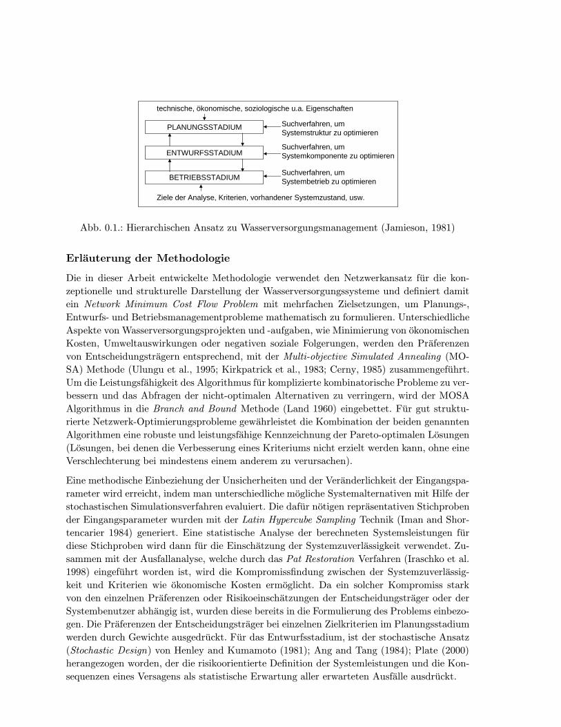
Um zwischen den vielfaltigen Tatigkeiten im Rahmen des Managements von Wasserversor-
gungssystemen unterscheiden zu konnen, wird haufig der von Jamieson (1981) entwickelte
Ansatz verwendet. Dieser unterscheidet Planungs-, Entwurfs- und Betriebsstadium (Abbil-
dung 0.1). Außerdem wird die Systemanalyse hier als ”Suchverfahren, um ein System zu opti-
mieren”gesehen, wo: a) die Planung sich auf die Entwicklung der Systemstruktur konzentriert,
b) der Entwurf optimale Systemkomponenten definiert, um die erforderte Systemleistungen
zu erfullen und c) im Betriebsstadium Haltungskosten optimiert, Instandhaltungsstrategien
entwickelt und Systemsleistungen verbessert werden.
PLANUNGSSTADIUM
ENTWURFSSTADIUM
BETRIEBSSTADIUM
technische, ökonomische, soziologische u.a. Eigenschaften
Suchverfahren, um Systemstruktur zu optimieren
Suchverfahren, um Systemkomponente zu optimieren
Suchverfahren, um Systembetrieb zu optimieren
Ziele der Analyse, Kriterien, vorhandener Systemzustand, usw.
Abb. 0.1.: Hierarchischen Ansatz zu Wasserversorgungsmanagement (Jamieson, 1981)
Erlauterung der Methodologie
Die in dieser Arbeit entwickelte Methodologie verwendet den Netzwerkansatz fur die kon-
zeptionelle und strukturelle Darstellung der Wasserversorgungssysteme und definiert damit
ein Network Minimum Cost Flow Problem mit mehrfachen Zielsetzungen, um Planungs-,
Entwurfs- und Betriebsmanagementprobleme mathematisch zu formulieren. Unterschiedliche
Aspekte von Wasserversorgungsprojekten und -aufgaben, wie Minimierung von okonomischen
Kosten, Umweltauswirkungen oder negativen soziale Folgerungen, werden den Praferenzen
von Entscheidungstragern entsprechend, mit der Multi-objective Simulated Annealing (MO-
SA) Methode (Ulungu et al., 1995; Kirkpatrick et al., 1983; Cerny, 1985) zusammengefuhrt.
Um die Leistungsfahigkeit des Algorithmus fur komplizierte kombinatorische Probleme zu ver-
bessern und das Abfragen der nicht-optimalen Alternativen zu verringern, wird der MOSA
Algorithmus in die Branch and Bound Methode (Land 1960) eingebettet. Fur gut struktu-
rierte Netzwerk-Optimierungsprobleme gewahrleistet die Kombination der beiden genannten
Algorithmen eine robuste und leistungsfahige Kennzeichnung der Pareto-optimalen Losungen
(Losungen, bei denen die Verbesserung eines Kriteriums nicht erzielt werden kann, ohne eine
Verschlechterung bei mindestens einem anderem zu verursachen).
Eine methodische Einbeziehung der Unsicherheiten und der Veranderlichkeit der Eingangspa-
rameter wird erreicht, indem man unterschiedliche mogliche Systemalternativen mit Hilfe der
stochastischen Simulationsverfahren evaluiert. Die dafur notigen reprasentativen Stichproben
der Eingangsparameter wurden mit der Latin Hypercube Sampling Technik (Iman and Shor-
tencarier 1984) generiert. Eine statistische Analyse der berechneten Systemsleistungen fur
diese Stichproben wird dann fur die Einschatzung der Systemzuverlassigkeit verwendet. Zu-
sammen mit der Ausfallanalyse, welche durch das Pat Restoration Verfahren (Iraschko et al.
1998) eingefuhrt worden ist, wird die Kompromissfindung zwischen der Systemzuverlassig-
keit und Kriterien wie okonomische Kosten ermoglicht. Da ein solcher Kompromiss stark
von den einzelnen Praferenzen oder Risikoeinschatzungen der Entscheidungstrager oder der
Systembenutzer abhangig ist, wurden diese bereits in die Formulierung des Problems einbezo-
gen. Die Praferenzen der Entscheidungstrager bei einzelnen Zielkriterien im Planungsstadium
werden durch Gewichte ausgedruckt. Fur das Entwurfsstadium, ist der stochastische Ansatz
(Stochastic Design) von Henley and Kumamoto (1981); Ang and Tang (1984); Plate (2000)
herangezogen worden, der die risikoorientierte Definition der Systemleistungen und die Kon-
sequenzen eines Versagens als statistische Erwartung aller erwarteten Ausfalle ausdruckt.
Die beschriebene Methodologie wurde in drei entsprechenden Computermodellen umgesetzt.
Sie sind an die spezifischen Aspekte der Wasserversorgungsplanung, des Entwurfes und des
Betriebsmanagements angepasst und ermoglichen im Verbund eine volle Entscheidungsunter-
stutzung im Management von Wasserversorgungssystemen.
Erlauterung der Modellen
Die Struktur der drei Teilmodelle und die durch sie berechneten Ergebnisse werden in dieser
Ubersicht prinzipiell angand von Fallstudien erlautert, die in der Arbeit im Detail dargestellt
und anusgewartet werden. Dieses Vorgeben scheint am besten geeignet, um einen rascher
Uberblick uber die Zielsetzung, die Vergehensweise, die Leistungen und den Anwendungsnut-
zen der Modelle zu geben
Das Planungsmodell
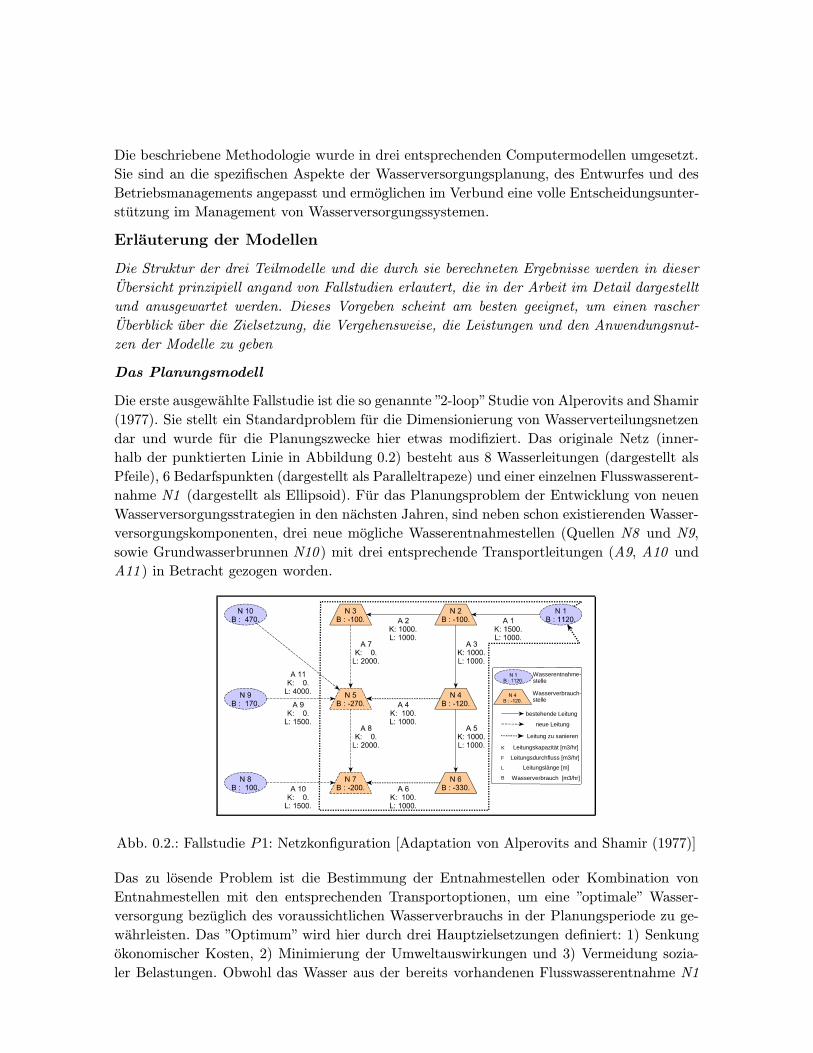
Die erste ausgewahlte Fallstudie ist die so genannte ”2-loop”Studie von Alperovits and Shamir
(1977). Sie stellt ein Standardproblem fur die Dimensionierung von Wasserverteilungsnetzen
dar und wurde fur die Planungszwecke hier etwas modifiziert. Das originale Netz (inner-
halb der punktierten Linie in Abbildung 0.2) besteht aus 8 Wasserleitungen (dargestellt als
Pfeile), 6 Bedarfspunkten (dargestellt als Paralleltrapeze) und einer einzelnen Flusswasserent-
nahme N1 (dargestellt als Ellipsoid). Fur das Planungsproblem der Entwicklung von neuen
Wasserversorgungsstrategien in den nachsten Jahren, sind neben schon existierenden Wasser-
versorgungskomponenten, drei neue mogliche Wasserentnahmestellen (Quellen N8 und N9,
sowie Grundwasserbrunnen N10 ) mit drei entsprechende Transportleitungen (A9, A10 und
A11 ) in Betracht gezogen worden.
Wasserverbrauch-stelle
Wasserentnahme-stelle
Wasserverbrauch [m3/hr]B
Leitung zu sanieren
neue Leitung
bestehende Leitung
K Leitungskapazität [m3/hr]
F
L
Leitungsdurchfluss [m3/hr]
Leitungslänge [m]
Abb. 0.2.: Fallstudie P1: Netzkonfiguration [Adaptation von Alperovits and Shamir (1977)]
Das zu losende Problem ist die Bestimmung der Entnahmestellen oder Kombination von
Entnahmestellen mit den entsprechenden Transportoptionen, um eine ”optimale” Wasser-
versorgung bezuglich des voraussichtlichen Wasserverbrauchs in der Planungsperiode zu ge-
wahrleisten. Das ”Optimum” wird hier durch drei Hauptzielsetzungen definiert: 1) Senkung
okonomischer Kosten, 2) Minimierung der Umweltauswirkungen und 3) Vermeidung sozia-
ler Belastungen. Obwohl das Wasser aus der bereits vorhandenen Flusswasserentnahme N1
sehr kostengunstig transportiert werden kann, haben große Entnahmen negative Auswirkun-
gen fur das Flussokosystem. Andererseits ermoglichen das Quell- und Grundwasser (N8, N9,
N10 ) eine bessere Verteilung der Umweltbelastung, sind aber mit großen Investitionskosten
verbunden. Zusatzlich wird das Grundwasser als strategische Wasserressource angesehen und
große Entnahmewerte konnen negative soziale Folgen haben.
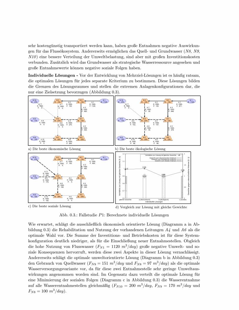
Individuelle Losungen - Vor der Entwicklung von Mehrziel-Losungen ist es haufig ratsam,
die optimalen Losungen fur jedes separate Kriterium zu bestimmen. Diese Losungen bilden
die Grenzen des Losungsraumes und stellen die extremen Anlagenkonfigurationen dar, die
nur eine Zielsetzung bevorzugen (Abbildung 0.3).
a) Die beste okonomische Losung
b) Die beste okologische Losung
c) Die beste soziale Losung
0.6
0.7
0.8
0.9
1
1.1
1.2
gleiche Gewichte a (ökonoimisch) b (ökologisch) c (soziale) 0
0.5
1
1.5
2
Ver
hältn
is z
ur L
ösun
g m
it gl
eich
er G
ewic
hte
[0..1
]
Gew
icht
e ge
gen
unte
rsch
iedl
iche
Krit
erie
n [0
..1]
Individuelle Lösungen
1.00.99
0.89
0.96
Verhältnis zur Lösung mit gleicher Gewichte
Gewicht zum ökonomischen KriteriumGewicht zum ökologische Kriterium
Gewicht zum soziale Kriterium
d) Vergleich zur Losung mit gleiche Gewichte
Abb. 0.3.: Fallstudie P1: Berechnete individuelle Losungen
Wie erwartet, schlagt die ausschließlich okonomisch orientierte Losung (Diagramm a in Ab-
bildung 0.3) die Rehabilitation und Nutzung der vorhandenen Leitungen A4 und A6 als die
optimale Wahl vor. Die Summe der Investitions- und Betriebskosten ist fur diese System-
konfiguration deutlich niedriger, als fur die Einschließung neuer Entnahmestellen. Obgleich
die hohe Nutzung von Flusswasser (FN1 = 1120 m3/day) große negative Umwelt- und so-
ziale Konsequenzen hervorruft, werden diese zwei Aspekte in dieser Losung vernachlassigt.
Andererseits schlagt die optimale umweltorientierte Losung (Diagramm b in Abbildung 0.3)
den Gebrauch von Quellwasser (FN9 = 151 m3/day und FN8 = 97 m3/day) als die optimale
Wasserversorgungsvariante vor, da fur diese zwei Entnahmestelle sehr geringe Umweltaus-
wirkungen angenommen worden sind. Im Gegensatz dazu verteilt die optimale Losung fur
eine Minimierung der sozialen Folgen (Diagramm c in Abbildung 0.3) die Wasserentnahme
auf alle Wasserentnahmestellen gleichmaßig (FN10 = 200 m3/day, FN9 = 170 m3/day und
FN8 = 100 m3/day).
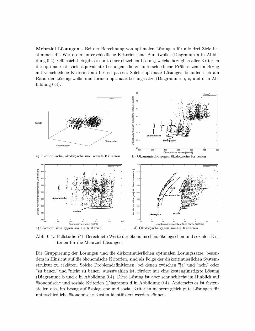
Mehrziel Losungen - Bei der Berechnung von optimalen Losungen fur alle drei Ziele be-
stimmen die Werte der unterschiedliche Kriterien eine Punktwolke (Diagramm a in Abbil-
dung 0.4). Offensichtlich gibt es statt einer einzelnen Losung, welche bezuglich aller Kriterien
die optimale ist, viele aquivalente Losungen, die zu unterschiedliche Praferenzen im Bezug
auf verschiedene Kriterien am besten passen. Solche optimale Losungen befinden sich am
Rand der Losungswolke und formen optimale Losungssatze (Diagramme b, c, und d in Ab-
bildung 0.4).
Soziale
Lösung
Ökonomische
Ökologische
Soziale
a) Okonomische, okologische und soziale Kriterien
45
50
55
60
65
70
75
80
200 300 400 500 600 700 800
Um
wel
taus
wirk
unge
n [b
etro
ffene
Fla
che
1000
Ha]
Ökonomische Kosten [1000$]
Lösung
ökologische
ökonomische
b) Okonomische gegen okologische Kriterien
340
345
350
355
360
365
370
375
380
200 300 400 500 600 700 800
Soz
iale
Aus
wirk
unge
n [b
etro
ffene
Gem
eind
en]
Ökonomische Kosten [1000$]
Lösung
ökonomische
soziale
c) Okonomische gegen soziale Kriterien
340
345
350
355
360
365
370
375
380
45 50 55 60 65 70 75 80
Soz
iale
Aus
wirk
unge
n [b
etro
ffene
Gem
eind
en]
Umweltauswirkungen [betroffene Flache 1000Ha]
Lösung
ökonomische
ökologisce soziale
. d) Okologische gegen soziale Kriterien
Abb. 0.4.: Fallstudie P1: Berechnete Werte der okonomischen, okologischen und sozialen Kri-
terien fur die Mehrziel-Losungen
Die Gruppierung der Losungen und die diskontinuierlichen optimalen Losungssatze, beson-
ders in Hinsicht auf die okonomische Kriterien, sind als Folge der diskontinuierlichen System-
struktur zu erklaren. Solche Problemdefinitionen, bei denen zwischen ”ja” und ”nein” oder
”zu bauen” und ”nicht zu bauen” auszuwahlen ist, fordert nur eine kostengunstigste Losung
(Diagramme b und c in Abbildung 0.4). Diese Losung ist aber sehr schlecht im Hinblick auf
okonomische und soziale Kriterien (Diagramm d in Abbildung 0.4). Anderseits es ist festzu-
stellen dass im Bezug auf okologische und sozial Kriterien mehrere gleich gute Losungen fur
unterschiedliche okonomische Kosten identifiziert werden konnen.

Das Entwurfsmodell
Die Entwurfsanalyse ist eine Fortsetzung der Planungsanalyse, in der die Kapazitaten der
Netzelemente fur die ausgewahlte optimale Netzkonfiguration festgestellt werden sollen. Die-
jenige Netzkonfiguration, die im Bezug auf soziale Kriterien optimal ist und alle drei neue
Wasserentnahmestellen (N8, N9 und N10 ) bevorzugt, wird hier vom Entwurfsstandpunkt aus
optimiert. Zu optimieren sind die Netzdurchflusse und -durchmesser die minimale Investitions-
und Betriebskosten haben aber trotzdem ein bestimmten Niveau von Systemzuverlassigkeit
gewahrleisten. Die Systemzuverlassigkeit wurde durch Analysieren von Systemverhalten unter
Berucksichtigung von mogliche Ausfalle der individuelle Systemkomponenten und unter Be-
rucksichtigung von Unsicherheiten in den Eingabeparametern (z.B. Wasserbedarf ) bestimmt.
Die kostengunstigste Losung wurde zuerst berechnet. Die standardmaßigen Leitungsdurch-
messer und die entsprechenden Investitions- und Betriebskosten wurden aus der Studie von
Alperovits and Shamir (1977) entnommen. Die berechneten optimalen Netzdurchflusse und
die entsprechenden kostengunstigsten Netzdurchmesser, die fur den Transport der erforder-
lichen Wassermengen und einen minimalen Druck von 30 m Wassersaule an jedem Bedarfs-
punkt erforderlich sind, sind in Tabelle 0.2 dargestellt. Diese Ergebnisse stimmen mit denen
anderer Studien, die sich mit dem gleichen Problem befasst haben und andere Optimie-
rungsverfahren verwendet haben z.B. Genetic Algorithm (Savic and Walters, 1997), Search
Algorithm (Abebe and Solomatine, 1998), Simulated Annealing (Cunha and Sousa, 1999),
Shuffled Frog Leaping (Eusuff and Lansey, 2003) und Shuffled Complex Evolution (Liong and
Atiquzzaman, 2004) uberein.
1 1000 130 650.00 2.46 18 457.22 1000 130 100.00 1.35 10 254.03 1000 130 450.00 2.21 16 406.44 1000 130 0.00 0.00 6 152.45 1000 130 330.00 1.25 16 406.46 1000 130 0.00 0.00 6 152.48 2000 130 100.00 7.99 8 203.29 1500 130 170.00 5.40 10 254.0
10 1500 130 100.00 5.99 8 203.211 4000 130 200.00 8.00 12 304.8
Durchmesser [inch]
Durchmesser [m]
Länge [m]
Reibungskoeffizient
Durchfluss [m3/day]
Druckverlust [m]
Rohre
1 150 180.00 30.002 120 177.54 57.543 130 176.19 46.194 125 175.33 50.335 120 175.33 55.336 135 174.08 39.087 130 167.34 37.348 150 180.00 30.009 150 180.00 30.00
10 150 180.00 30.00
Geodet. Höhe [m]
Energie Höhe [m]
Druck [m]Knoten
Tab. 0.2.: Fallstudie D1: Berechnete optimale Durchflusse, Druck und Druckverluste
Obwohl optimal angesichts der okonomischen Kosten, bietet diese Losung sehr wenig Zuver-
lassigkeit und Sicherheit im Betrieb und ist von geringem praktischen Wert. Deshalb wird
dieser Ein-Kriterium Entwurfsansatz um eine Ausfall- und Unsicherheitsanalyse erweitert.
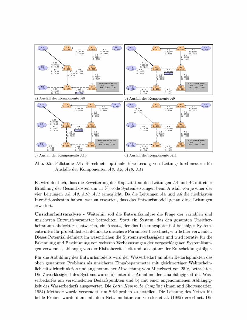
Ausfallanalyse - Die Entwurfsanalyse muss in der Lage sein, eine Reihe von Betriebszustan-
den anzusprechen, wobei der Ausfall eines beliebigen Netzbestandteils ein Standardproblem
darstellt. Die hier verwendete Methode fur die systematische Erweiterungen der System-
kapazitat basiert auf der Path Restoreation Methode von Iraschko and Grover (2000). Die
Ergebnisse der Ausfallanalysen fur alle Leitungen (A8, A9, A10, A11 ) die das Wasser zu
den Verbrauchern N5 und N7 liefern und die resultierenden Zunahmen der Netzdurchmesser
werden in Abbildung 0.5 dargestellt.
KOSTENERHÖHUNG
a) Ausfall der Komponente A8
KOSTENERHÖHUNG
b) Ausfall der Komponente A9
KOSTENERHÖHUNG
c) Ausfall der Komponente A10
KOSTENERHÖHUNG
d) Ausfall der Komponente A11
Abb. 0.5.: Fallstudie D1: Berechnete optimale Erweiterung von Leitungsdurchmessern fur
Ausfalle der Komponenten A8, A9, A10, A11
Es wird deutlich, dass die Erweiterung der Kapazitat an den Leitungen A4 und A6 mit einer
Erhohung der Gesamtkosten um 11 %, volle Systemleistungen beim Ausfall von je einer der
vier Leitungen A8, A9, A10, A11 ermoglicht. Da die Leitungen A4 und A6 die niedrigsten
Investitionskosten haben, war zu erwarten, dass das Entwurfsmodell genau diese Leitungen
erweitert.
Unsicherheitsanalyse - Weiterhin soll die Entwurfsanalyse die Frage der variablen und
unsicheren Entwurfsparameter betrachten. Statt ein System, das den gesamten Unsicher-
heitsraum abdeckt zu entwerfen, ein Ansatz, der das Leistungspotential beliebiges System-
entwurfes fur probabilistisch definierte unsichere Parameter berechnet, wurde hier verwendet.
Dieses Potential definiert im wesentlichen die Systemzuverlassigkeit und wird iterativ fur die
Erkennung und Bestimmung von weiteren Verbesserungen der vorgeschlagenen Systemlosun-
gen verwendet, abhangig von der Risikobereitscheft und -akzeptanz der Entscheidungstrager.
Fur die Abbildung des Entwurfsmodells wird der Wasserbedarf an allen Bedarfspunkten des
oben genannten Problems als unsicherer Eingabeparameter mit gleichwertiger Wahrschein-
lichkeitsdichtefunktion und angenommener Abweichung vom Mittelwert von 25 % betrachtet.
Die Zuverlassigkeit des Systems wurde a) unter der Annahme der Unabhangigkeit des Was-
serbedarfes am verschiedenen Bedarfspunkten und b) mit einer angenommenen Abhangig-
keit des Wasserbedarfs ausgewertet. Die Latin Hypercube Sampling (Iman and Shortencarier,
1984) Methode wurde verwendet, um Stichproben zu erstellen. Die Leistung des Netzes fur
beide Proben wurde dann mit dem Netzsimulator von Gessler et al. (1985) errechnet. Die
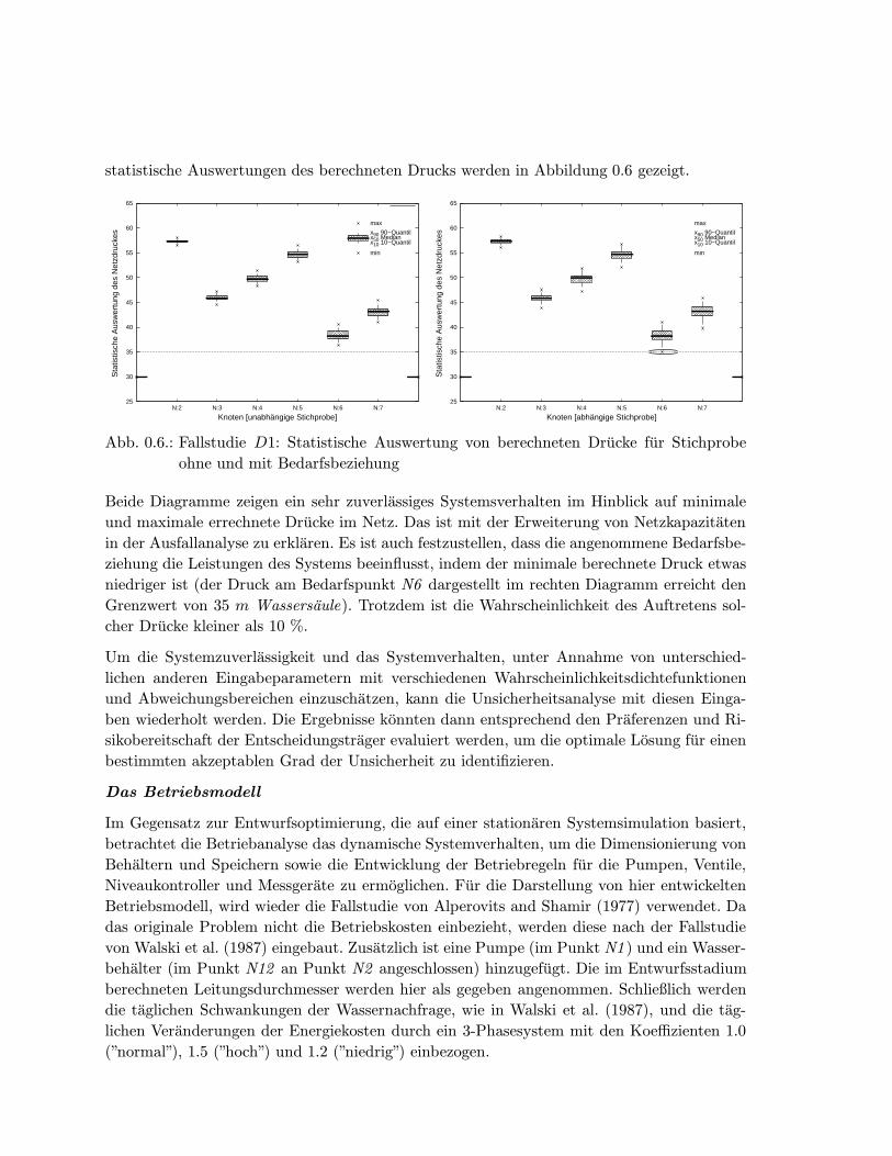
statistische Auswertungen des berechneten Drucks werden in Abbildung 0.6 gezeigt.
25
30
35
40
45
50
55
60
65
N:2 N:3 N:4 N:5 N:6 N:7
Sta
tistis
che
Aus
wer
tung
des
Net
zdru
ckes
Knoten [unabhängige Stichprobe]
min
x10 10−Quantilx50 Medianx90 90−Quantil
max
25
30
35
40
45
50
55
60
65
N:2 N:3 N:4 N:5 N:6 N:7
Sta
tistis
che
Aus
wer
tung
des
Net
zdru
ckes
Knoten [abhängige Stichprobe]
min
x10 10−Quantilx50 Medianx90 90−Quantil
max
Abb. 0.6.: Fallstudie D1: Statistische Auswertung von berechneten Drucke fur Stichprobe
ohne und mit Bedarfsbeziehung
Beide Diagramme zeigen ein sehr zuverlassiges Systemsverhalten im Hinblick auf minimale
und maximale errechnete Drucke im Netz. Das ist mit der Erweiterung von Netzkapazitaten
in der Ausfallanalyse zu erklaren. Es ist auch festzustellen, dass die angenommene Bedarfsbe-
ziehung die Leistungen des Systems beeinflusst, indem der minimale berechnete Druck etwas
niedriger ist (der Druck am Bedarfspunkt N6 dargestellt im rechten Diagramm erreicht den
Grenzwert von 35 m Wassersaule). Trotzdem ist die Wahrscheinlichkeit des Auftretens sol-
cher Drucke kleiner als 10 %.
Um die Systemzuverlassigkeit und das Systemverhalten, unter Annahme von unterschied-
lichen anderen Eingabeparametern mit verschiedenen Wahrscheinlichkeitsdichtefunktionen
und Abweichungsbereichen einzuschatzen, kann die Unsicherheitsanalyse mit diesen Einga-
ben wiederholt werden. Die Ergebnisse konnten dann entsprechend den Praferenzen und Ri-
sikobereitschaft der Entscheidungstrager evaluiert werden, um die optimale Losung fur einen
bestimmten akzeptablen Grad der Unsicherheit zu identifizieren.
Das Betriebsmodell
Im Gegensatz zur Entwurfsoptimierung, die auf einer stationaren Systemsimulation basiert,
betrachtet die Betriebanalyse das dynamische Systemverhalten, um die Dimensionierung von
Behaltern und Speichern sowie die Entwicklung der Betriebregeln fur die Pumpen, Ventile,
Niveaukontroller und Messgerate zu ermoglichen. Fur die Darstellung von hier entwickelten
Betriebsmodell, wird wieder die Fallstudie von Alperovits and Shamir (1977) verwendet. Da
das originale Problem nicht die Betriebskosten einbezieht, werden diese nach der Fallstudie
von Walski et al. (1987) eingebaut. Zusatzlich ist eine Pumpe (im Punkt N1 ) und ein Wasser-
behalter (im Punkt N12 an Punkt N2 angeschlossen) hinzugefugt. Die im Entwurfsstadium
berechneten Leitungsdurchmesser werden hier als gegeben angenommen. Schließlich werden
die taglichen Schwankungen der Wassernachfrage, wie in Walski et al. (1987), und die tag-
lichen Veranderungen der Energiekosten durch ein 3-Phasesystem mit den Koeffizienten 1.0
(”normal”), 1.5 (”hoch”) und 1.2 (”niedrig”) einbezogen.
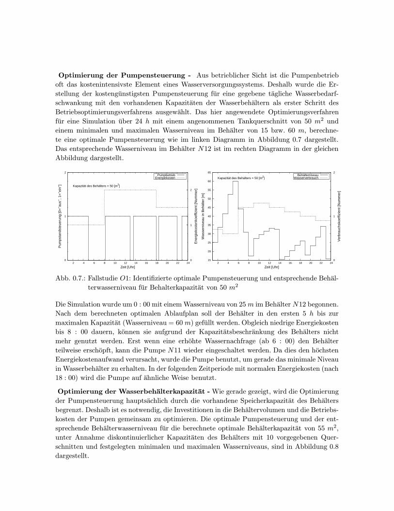
Optimierung der Pumpensteuerung - Aus betrieblicher Sicht ist die Pumpenbetrieb
oft das kostenintensivste Element eines Wasserversorgungssystems. Deshalb wurde die Er-
stellung der kostengunstigsten Pumpensteuerung fur eine gegebene tagliche Wasserbedarf-
schwankung mit den vorhandenen Kapazitaten der Wasserbehaltern als erster Schritt des
Betriebsoptimierungsverfahrens ausgewahlt. Das hier angewendete Optimierungsverfahren
fur eine Simulation uber 24 h mit einem angenommenen Tankquerschnitt von 50 m2 und
einem minimalen und maximalen Wasserniveau im Behalter von 15 bzw. 60 m, berechne-
te eine optimale Pumpensteuerung wie im linken Diagramm in Abbildung 0.7 dargestellt.
Das entsprechende Wasserniveau im Behalter N12 ist im rechten Diagramm in der gleichen
Abbildung dargestellt.
0
1
2
2 4 6 8 10 12 14 16 18 20 22 24 0
1
2
Pum
psta
ndst
euer
ung
[0=
’’aus
’’, 1
=’’e
in’’]
Ene
rgie
kost
enko
effiz
ient
[Num
mer
]
Zeit [Uhr]
Kapazität des Behälters = 50 [m2]
PumpbetriebEnergiekosten
15
20
25
30
35
40
45
50
55
60
65
2 4 6 8 10 12 14 16 18 20 22 24 0
1
2
Was
sern
ivea
u in
Beh
älte
r [m
]
Ver
brau
chsk
oeffi
zien
t [N
umm
er]
Zeit [Uhr]
Kapazität des Behälters = 50 [m2]Behälterniveau
Wasserverbrauch
Abb. 0.7.: Fallstudie O1: Identifizierte optimale Pumpensteuerung und entsprechende Behal-
terwasserniveau fur Behalterkapazitat von 50 m2
Die Simulation wurde um 0 : 00 mit einemWasserniveau von 25m im Behalter N12 begonnen.
Nach dem berechneten optimalen Ablaufplan soll der Behalter in den ersten 5 h bis zur
maximalen Kapazitat (Wasserniveau = 60m) gefullt werden. Obgleich niedrige Energiekosten
bis 8 : 00 dauern, konnen sie aufgrund der Kapazitatsbeschrankung des Behalters nicht
mehr genutzt werden. Erst wenn eine erhohte Wassernachfrage (ab 6 : 00) den Behalter
teilweise erschopft, kann die Pumpe N11 wieder eingeschaltet werden. Da dies den hochsten
Energiekostenaufwand verursacht, wurde die Pumpe benutzt, um gerade das minimale Niveau
in Wasserbehalter zu erhalten. In der folgenden Zeitperiode mit normalen Energiekosten (nach
18 : 00) wird die Pumpe auf ahnliche Weise benutzt.
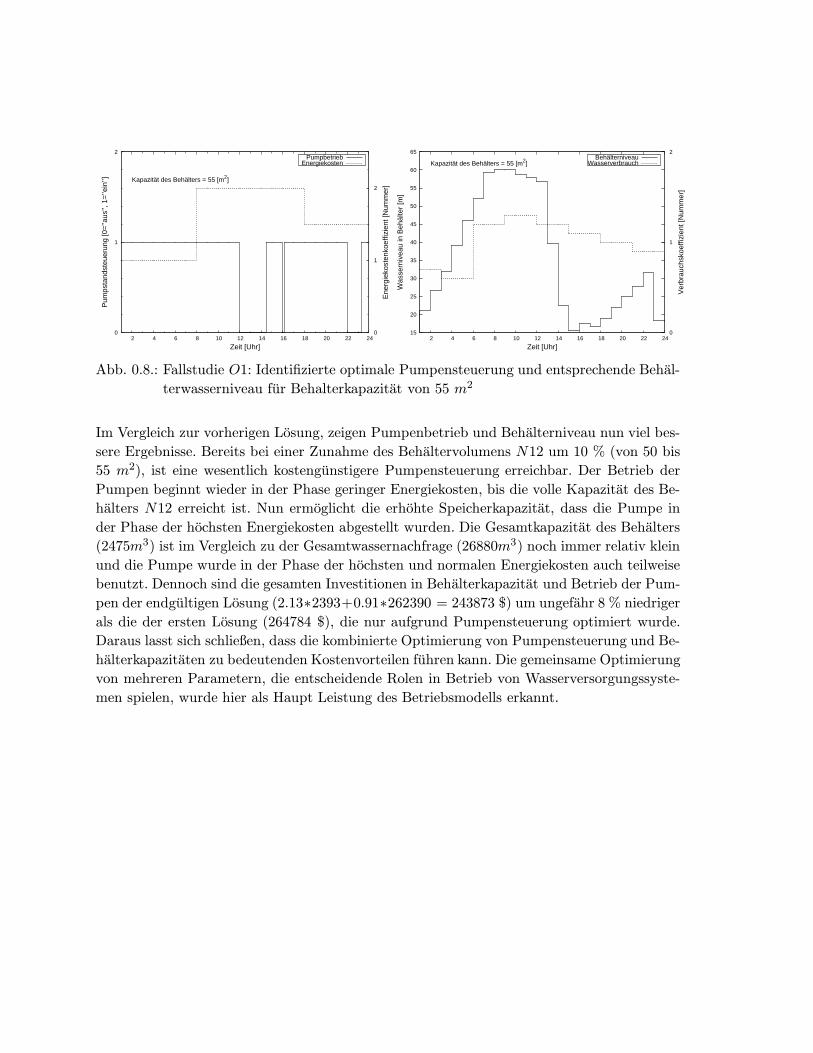
Optimierung der Wasserbehalterkapazitat - Wie gerade gezeigt, wird die Optimierung
der Pumpensteuerung hauptsachlich durch die vorhandene Speicherkapazitat des Behalters
begrenzt. Deshalb ist es notwendig, die Investitionen in die Behaltervolumen und die Betriebs-
kosten der Pumpen gemeinsam zu optimieren. Die optimale Pumpensteuerung und der ent-
sprechende Behalterwasserniveau fur die berechnete optimale Behalterkapazitat von 55 m2,
unter Annahme diskontinuierlicher Kapazitaten des Behalters mit 10 vorgegebenen Quer-
schnitten und festgelegten minimalen und maximalen Wasserniveaus, sind in Abbildung 0.8
dargestellt.
0
1
2
2 4 6 8 10 12 14 16 18 20 22 24 0
1
2
Pum
psta
ndst
euer
ung
[0=
’’aus
’’, 1
=’’e
in’’]
Ene
rgie
kost
enko
effiz
ient
[Num
mer
]
Zeit [Uhr]
Kapazität des Behälters = 55 [m2]
PumpbetriebEnergiekosten
15
20
25
30
35
40
45
50
55
60
65
2 4 6 8 10 12 14 16 18 20 22 24 0
1
2
Was
sern
ivea
u in
Beh
älte
r [m
]
Ver
brau
chsk
oeffi
zien
t [N
umm
er]
Zeit [Uhr]
Kapazität des Behälters = 55 [m2]Behälterniveau
Wasserverbrauch
Abb. 0.8.: Fallstudie O1: Identifizierte optimale Pumpensteuerung und entsprechende Behal-
terwasserniveau fur Behalterkapazitat von 55 m2
Im Vergleich zur vorherigen Losung, zeigen Pumpenbetrieb und Behalterniveau nun viel bes-
sere Ergebnisse. Bereits bei einer Zunahme des Behaltervolumens N12 um 10 % (von 50 bis
55 m2), ist eine wesentlich kostengunstigere Pumpensteuerung erreichbar. Der Betrieb der
Pumpen beginnt wieder in der Phase geringer Energiekosten, bis die volle Kapazitat des Be-
halters N12 erreicht ist. Nun ermoglicht die erhohte Speicherkapazitat, dass die Pumpe in
der Phase der hochsten Energiekosten abgestellt wurden. Die Gesamtkapazitat des Behalters
(2475m3) ist im Vergleich zu der Gesamtwassernachfrage (26880m3) noch immer relativ klein
und die Pumpe wurde in der Phase der hochsten und normalen Energiekosten auch teilweise
benutzt. Dennoch sind die gesamten Investitionen in Behalterkapazitat und Betrieb der Pum-
pen der endgultigen Losung (2.13∗2393+0.91∗262390 = 243873 $) um ungefahr 8 % niedriger
als die der ersten Losung (264784 $), die nur aufgrund Pumpensteuerung optimiert wurde.
Daraus lasst sich schließen, dass die kombinierte Optimierung von Pumpensteuerung und Be-
halterkapazitaten zu bedeutenden Kostenvorteilen fuhren kann. Die gemeinsame Optimierung
von mehreren Parametern, die entscheidende Rolen in Betrieb von Wasserversorgungssyste-
men spielen, wurde hier als Haupt Leistung des Betriebsmodells erkannt.

Kurzfassung und Ausblick
In der vorliegenden Arbeit wurde eine Methodologie fur die integrative Entscheidungsunter-
stutzung in Management von Wasserversorgungssystemen entwickelt und in drei Modellen
(Planungs-, Entwurfs- und Betriebsmodell) eingebaut. Das Planungsmodell integriert techni-
sche, okologische und soziookonomische Aspekte, die fur die Auswahl der Wasserentnahmen,
die Aufbereitung und den Transport zu den Wasserverbrauchern relevant sind und ermittelt
eine Auswahl von moglichen Systemkonfigurationen, die fur verschiedene Kombinationen von
Entscheidungstrager-Praferenzen optimiert sind. Das Entwurfsmodell dient der Dimensionie-
rung der Komponenten der Wasserversorgungssysteme, die ein im Bezug auf okonomische
Kosten und Zuverlassigkeit optimiertes Systems darstellen. Eine Ausfallanalyse und eine
Analyse der Parameterunsicherheiten (z.B. prognostizierter Wasserbedarf) sind im Modell
vorhanden und dienen einer risikoorientierten Abgrenzung von moglichen Entwurfsvarianten.
Das Betriebsmodell identifiziert die optimale Große von Wasserspeicheranlagen und den op-
timalen Betriebsplan von Pumpenanlagen, die gleichzeitig minimale Investitionskosten und
Betriebskosten haben.
Alle drei Modelle basieren auf der Netzwerk-Reprasentation von Wasserversorgungsstruktur
und -funktion und auf einer Kombination von Simulated Annealing und Branch and Bound
Algorithmen zur Losung des Minimum Cost Network Flow Problems. Fortgeschrittene Path
Restoration und Latin Hypercube Sampling Methoden wurden fur die Betriebssicherheit und
Unsicherheitsanalyse benutzt. Alle Methoden wurden fur Wasserversorgungssysteme ange-
passt und mit zwei existierenden theoretischen Fallstudien verglichen. Die Ergebnisse sind
sehr plausibel und die angewendeten Methoden haben ein hohe Effizienz. Die Entwicklung
einer einzigartigen Methodologie fur die Identifizierung von optimalen Planungs-, Entwurfs-
und Betriebsoptionen unter Berucksichtigung von unterschiedlichen Zielsetzungen und Krite-
rien, Betrachtung von Unsicherheiten sowie Integration von verschiedenen Systemparametern
wird als wesentliche Forschungsbeitrag angesehen.
Eine ausfuhrlichere Prufung und Validierung der Modelle ist ein erste notwendiger Schritt vor
der Anwendung. Die Anwendung der Modelle auf konkrete Fallstudien und die Diskussion
der Ergebnisse mit Experten aus der Praxis ist erforderlich. Es muss auch erwahnt werden,
dass die Vorauswahl einzelner Methoden fur die Losung des Netzproblems bezuglich der
Mehrziel-Optimierung, Unsicherheit der Eingabeparameter und Zuverlassigkeit des Systems
im Vergleich zu eine integrativen Betrachtung dieser Aufgaben innerhalb gut strukturierte
und definierte Planungs-, Entwurfs- und Betriebsprobleme, von geringere Wert ist. Damit
bleiben die hier angewendeten Methoden austauschbar, solange die Leistungsfahigkeit, die
Anwendbarkeit oder die Transparenz der Methodologie gewahrleistet ist.

1. Introduction
The following chapter introduces the motivation for this study, states the problems that are
aimed at and defines the research objectives. It concludes with a short description of the
structure of the study.
1.1. Motivation
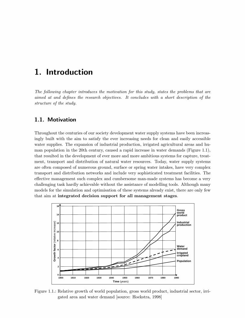
Throughout the centuries of our society development water supply systems have been increas-
ingly built with the aim to satisfy the ever increasing needs for clean and easily accessible
water supplies. The expansion of industrial production, irrigated agricultural areas and hu-
man population in the 20th century, caused a rapid increase in water demands (Figure 1.1),
that resulted in the development of ever more and more ambitious systems for capture, treat-
ment, transport and distribution of natural water resources. Today, water supply systems
are often composed of numerous ground, surface or spring water intakes, have very complex
transport and distribution networks and include very sophisticated treatment facilities. The
effective management such complex and cumbersome man-made systems has become a very
challenging task hardly achievable without the assistance of modelling tools. Although many
models for the simulation and optimisation of these systems already exist, there are only few
that aim at integrated decision support for all management stages.
Gro
wth
fac
tor
(rel
ativ
e in
crea
se)
Grossworldproduct
Industrialproduction
Waterdemand
Irrigatedcropland
Population
Time (years)1900 1910 1920 1930 1940 1950 1960 1970 1980 1990
0
2
4
6
8
10
12
14
16
Figure 1.1.: Relative growth of world population, gross world product, industrial sector, irri-
gated area and water demand [source: Hoekstra, 1998]
2 Introduction
The expanded use of natural water resources and the world wide pollution of this precious
asset left behind many contaminated natural water bodies and destroyed ecological habitats.
”The growing tension between intensive water use and the functioning of natural ecosystems
has shifted our perception of water supply systems from human utility services toward cou-
pled human-natural systems” (Allenby, 2004). The integrative consideration of the natural
environment and the human built-in systems has become our society’s new paradigm (IUCN
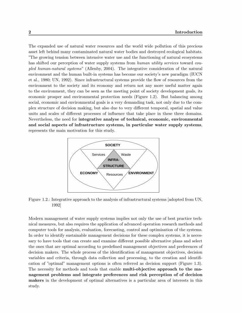
et al., 1980; UN, 1992). Since infrastructural systems provide the flow of resources from the
environment to the society and its economy and return not any more useful matter again
to the environment, they can be seen as the meeting point of society development goals, its
economic prosper and environmental protection needs (Figure 1.2). But balancing among
social, economic and environmental goals is a very demanding task, not only due to the com-
plex structure of decision making, but also due to very different temporal, spatial and value
units and scales of different processes of influence that take place in these three domains.
Nevertheless, the need for integrative analyse of technical, economic, environmental
and social aspects of infrastructure systems, in particular water supply systems,
represents the main motivation for this study.
SOCIETY
ECONOMY
INFRA-
STRUCTURE
ENVIRONMENT
Services Waste
Resources
SOCIETY
ECONOMY
INFRA-
STRUCTURE
ENVIRONMENT
Services Waste
Resources
Figure 1.2.: Integrative approach to the analysis of infrastructural systems [adopted from UN,
1992]
Modern management of water supply systems implies not only the use of best practice tech-
nical measures, but also requires the application of advanced operation research methods and
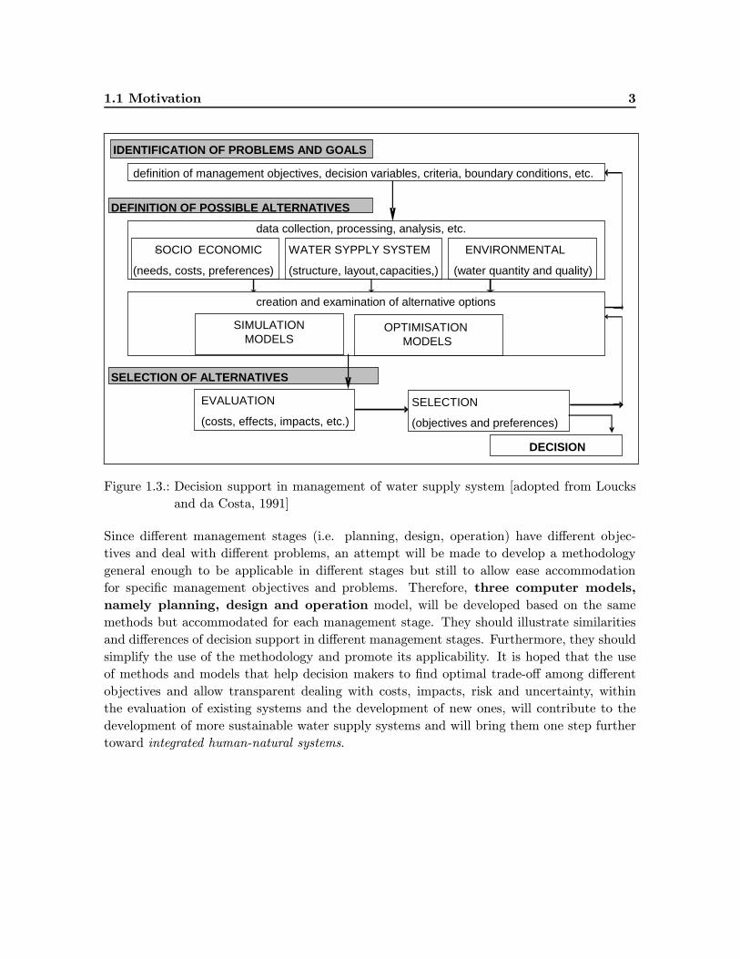
computer tools for analysis, evaluation, forecasting, control and optimisation of the systems.
In order to identify sustainable management decisions for these complex systems, it is neces-
sary to have tools that can create and examine different possible alternative plans and select
the ones that are optimal according to predefined management objectives and preferences of
decision makers. The whole process of the identification of management objectives, decision
variables and criteria, through data collection and processing, to the creation and identifi-
cation of ”optimal” management options is often referred as decision support (Figure 1.3).
The necessity for methods and tools that enable multi-objective approach to the ma-
nagement problems and integrate preferences and risk perception of of decision
makers in the development of optimal alternatives is a particular area of interests in this
study.
1.1 Motivation 3
OPTIMISATIONMODELS
DEFINITION OF POSSIBLE ALTERNATIVES
SELECTION OF ALTERNATIVES
SOCIO- ECONOMIC
(needs, costs, preferences)
WATER SYPPLY SYSTEM
(structure, layout,capacities,)
ENVIRONMENTAL
(water quantity and quality)
definition of management objectives, decision variables, criteria, boundary conditions, etc.
EVALUATION
(costs, effects, impacts, etc.)
SELECTION
(objectives and preferences)
DECISION
IDENTIFICATION OF PROBLEMS AND GOALS
data collection, processing, analysis, etc.
creation and examination of alternative options
SIMULATIONMODELS
Figure 1.3.: Decision support in management of water supply system [adopted from Loucks
and da Costa, 1991]
Since different management stages (i.e. planning, design, operation) have different objec-
tives and deal with different problems, an attempt will be made to develop a methodology
general enough to be applicable in different stages but still to allow ease accommodation
for specific management objectives and problems. Therefore, three computer models,
namely planning, design and operation model, will be developed based on the same
methods but accommodated for each management stage. They should illustrate similarities
and differences of decision support in different management stages. Furthermore, they should
simplify the use of the methodology and promote its applicability. It is hoped that the use
of methods and models that help decision makers to find optimal trade-off among different
objectives and allow transparent dealing with costs, impacts, risk and uncertainty, within
the evaluation of existing systems and the development of new ones, will contribute to the
development of more sustainable water supply systems and will bring them one step further
toward integrated human-natural systems.
4 Introduction
1.2. General Objectives and Current Problems of Interests
Following the ideas of sustainable development (IUCN et al., 1980; UN, 1992), the analysis
of water supply systems has to take into account all effects of intended activities on the
environmental and socioeconomic processes of importance. In addition the money and energy
flows as well as the social preferences that often govern these processes have to be considered
at the same time. The development of integrative methodologies for the joint analysis of
technical, environmental, economic and social aspects of water supply systems is the first
prerequisite for this. Therefore, the integration of different objectives and criteria in
the creation of alternative water supply management options is the prime problem
to be dealt with.
The importance of the stakeholders participation in the decision making process has been
recognized and already institutionally implemented in most of developed and many of de-
veloping countries (UNEC, 1998). For the management of water supply systems this means
not just better information of public and regulatory authorities about provided water ser-
vices, but also the participation of public, government, industry, environmentalists, and other
stakeholders. This increases not only the complexity of the decision making process but also
the importance of the formulation of alternative solutions that encompass interests
and objectives of different stakeholders and decision makers. The implementation
of the multi-criteria evaluation techniques in the analyses of water supply systems represents
the next milestone of this study.
The real life driving forces, such as different water needs, variable natural distribution of
water resources, various social and political preferences and different economic and technical
capabilities, led to the development of many different types of water supply systems. Al-
though these systems may differ in technical specifications, natural conveniences, form of
ownership or type of management body, under the current paradigm of the Integrated Wa-
ter Management (UNESCO, 1987) and the ever increasing standards for water quality and
control, even the smallest water supply systems can be hardly any more considered in iso-
lation. In addition, in the last decades, there is an obvious trend of mutual interconnecting
among water supply systems, due to the factors such as saving from the economy of scale,
increasing reliability of water supply, easier transfer of know-how and simpler regulatory con-
trol (Hirner, 2001 presents the performance assessment and Rott, 2005 and Rott, 2006 the
current trends in the water supply sector in Germany). Although many sophisticated mode-
lling tools for the analysis and management of such ever larger and complexer systems have
already been developed, very few have been practically implemented (Goulter, 1992; Walski,
1995). Accordingly, the problem with the analysis of water supply systems is not the lack
of appropriate tools, but rather a challenge to select methodologies that are able to han-
dle often very complex problems with simple enough and easily understandable
methods (Walski, 2001). The identification of such methodologies with the aim to increase
the understanding and applicability of the System Analysis techniques in the management of
water supply systems is intended to be the main practical contribution of this study.
1.2 General Objectives and Current Problems of Interests 5
In addition to the ever increasing spatial dimension of water supply systems, their inflexibility
poses even greater problem to their operators and managers. Water supply systems are typ-
ically designed for periods of 30 to 50 years and very often function much longer. Due to the
natural variability of most of their input parameters, their uncertain character and constant
changes in their environment, it happens quite often that water supply systems work under
different conditions than planned for majority of their life-time. For example many water
supply systems in developed countries operate in a low efficiency range due to the reduced
water consumption in last years (Tillman et al., 1999). In contrast, in developing countries,
majority of water suppliers still struggle to keep the peace with the rapidly increasing water
consumption. The physical changes in the systems characteristics due to corrosion, deposi-
tion, hydraulic stress, etc., additionally contribute to the variable and uncertain environment
in which the systems operate. Therefore a huge interest in the development of methodologies
for a more robust, flexible and reliable water supply systems planning, design and
operation with alternative options that are better accommodated for different possible de-
velopment scenarios exists. In particular, the incorporation of reliability in the water supply
system design is an important issue that will be addressed in this study.
There are many socioeconomic processes that influence the recent changes in the water sup-
ply sector. Liberalization and globalization of the water market, privatization of public water
companies, tighter environmental and water quality standards and greater environmental
awareness are just some of the pressures that dictate systems efficiency increase, cost saving,
environmental impacts attenuation and better accommodation to the users needs. Although,
water consumers are still accustomed to the very comprehensive services, and are still willing
to pay for them, it is reasonable to expect that their preferences, priorities and expectations
may also change in the near future. Since the traditional design approach, based on the use of
standards and codes of practice, is not able to account for variable system performance eval-
uation, the alternative approaches, such as Stochastic Design, have already been suggested.
Furthermore, novel approaches provide for the much more transparent and precise quantifica-
tion of the system uncertainty. The incorporation of the uncertainty considerations,
users’ and decision makers’ expectations and risk tolerance into the development
of alternative water supply systems planning, design and operation options is a
next important problem that this study aim at.
Finally, water supply is a very specific industry that is at the same time driven by the ”eq-
uity principle” and ”economic efficiency”. Water is a basic human need and the provision of
drinking water is mainly defined as a constitutional obligation of a state. In contrast, the
economic efficiency of water supply systems is an important factor that determine their fu-
ture development. Due to the fact that water users are connected to only one water supplier
there is no free water supply market that can regulate the water price by the principle of
offer and demand, the water suppliers are often strictly controlled by the authorities to meet
user demands at non-profit or low profit prices. In such a set-up, it is of prime importance to
provide for a sustainable decision making and active participation of all involved stakeholders.
Therefore the assessment of initial investments or production, maintenance and system ex-
pansion costs, as well as the assessment of the benefits of the water provision, have to be very
transparent, apparent and evident. Consequently, each step of the suggested methodology
has to be transparent and easily applicable to real-life water supply systems.
6 Introduction
1.3. Specific Objectives and the Aim of the Research
According to the general problems of interests stated above, a specific research objective of
this study is the development of a modelling methodology for the multi-objective
and risk-based decision support in planning, design and operation of water supply
systems. The methodology should be systematic, integrative, transparent, and applicable
to already existing water supply systems and new ones. In essence, the methodology should
be able to address the following issues:
1. Efficient modelling representation of the system characteristics,
2. Integration of multiple objectives and multiple preferences,
3. Integration of uncertainty, risk and reliability considerations.
As for any other study that aims to develop a methodology for the analysis of a real sys-
tem by replacing it with a model 1 the first obvious objective is to find an appropriate
conceptual and computational representation that will well enough substitute
not only the characteristics of water supply systems but also incorporate the
objectives and specifics of the management problems. As far as the characteristics
of water supply systems are concerned, beside their structural components such as intakes,
treatment plants, storage and delivery facilities with their characteristics such as locations,
flow capacities, pressure conditions, etc., the model has to represent the main processes such
as water withdrawal, transport, treatment, etc. and the different modes of operation such
as design conditions, normal operation and failure modes. Furthermore, a life time of water
supply systems consists of different management stages, such as planning, design, operation,
expansion, rehabilitation, that set up different objectives for the analysis. The methodology
should not only be flexible enough to accommodate for these different stages but it should
also encompass a wide range of combination of preferences toward different objectives that
can be set by different stakeholders and decision makers. Finally, in order to increase the
applicability of the suggested modelling methodology, it has to stay simple enough and easily
understandable.
Secondly the suggested methodology should provide for the integration of various ob-
jectives and criteria into analysis of water supply systems. Since there are a large
number of environmental and socioeconomic impacts and factors of influence, the most im-
portant ones have to be identified and their functional dependencies in terms of losses (costs)
and benefits (contributions) to and from water supply systems have to be quantified. Fur-
thermore, in order to integrate the functional relationships of different types of costs and
benefits (e.g. environmental losses due to water extraction, social benefits due to water pro-
vision, etc.) into one computational model, they have to be brought to same associate units
and scale. Since different decision makers have different preferences toward environmental,
economic or social criteria, the possibility to encompass such varying priorities has
to be provided. Furthermore, the methodology should provide for the trade-off among
1a theoretical construct that represents real life structures and processes with a set of variables and a set of
logical and quantitative relationships between them
1.4 Course of Action 7
different objectives with the aim to promote the identification of the alternatives that are
acceptable for all decision makers.
Lastly, the integration of uncertainty, risk and reliability considerations into eval-
uation of water supply systems performances is of a prime importance for the prac-
titioners. Unfortunately, knowing that most of the uncertainties such as data’s, system’s,
model’s uncertainties are inevitably connected with modelling, it is not to expect that the
”true” system performance can be assessed in advance. Still, the mediation of accessible un-
certainties represents the basis for robust and flexible system design. The traditional design
approach quantifies uncertainties based on standards and codes of practices and accounts for
them by adding some spare capacity in order to ”be on the safe side”. An intention of this
study is to offer a methodology that will evaluate the system performance for the recognized
level of input data uncertainty and quantify its reliability accordingly. In addition, the users’
and decision makers’ preferences and risk tolerance will be implemented in evaluation of sys-
tem’s performance in order to define ”how safe the system need to be”. Based on decision
makers’ risk acceptability, the statistical evaluation of system performances for large num-
ber of system simulations with uncertain parameters will yield reliability of a system. Such
calculated reliability may be then traded-off with other criteria such as economic costs or
environmental impacts.
1.4. Course of Action
The main building blocks of the presented study are arranged in three following chapters.
Chapter 2 - The Theoretical Foundations - defines the notation, introduces the main
characteristics of water supply systems and defines the main concepts necessary to achieve
the objectives of the study. Physical, socioeconomic and environmental characteristics as well
as uncertainty, risk and reliability issues of a prime importance are presented and discussed.
The hierarchical approach to the management of water supply systems is presented and the
suggested division into planning, design and operation stage is adopted. For each of these
stages a detailed literature review of the application of the System Analysis techniques is
provided and discussed with the aim to identify the starting point and the needed focus for
this study.
Chapter 3 - The Methodology Development - chapter aims to establish the theoretical
base for the development of a methodology that will enable integration of environmental,
economic and social aspects in water supply development as well as the uncertainty, risk and
reliability based assessment of water supply systems performances. In order to provide for
a good structural and functional representation of the systems, the methodology is based
on the Network Concept and combines the Graph Theory algorithms with the advanced
System Analysis optimisation methods to achieve the effective solution of the water supply
management problems. Suggested algorithms are accommodated to deal with water supply
planning, design and operation problem and implemented into corresponding models. Special
attention has been devoted to the multi-objectiveness, transparency and applicability of the
methodology.

8 Introduction
Chapter 4 - The Model Development and Application - chapter presents three
computer models based on the previously defined methodology. The planning model provides
for the integration of technical, economic, environmental and social objectives in the process
of development and selection of new water supply strategies (e.g. possible new sources,
allocation to demand centres, water transfer options, etc.). The participation of stakeholders
is assumed and the identification of the optimal systems configurations for different sets of
stakeholders preferences is aimed at. The design model deal with the minimum cost sizing of
water supply components and the system’s reliability issue. The deterministic design criteria
are combined with stochastic evaluation of the parameters’ uncertainty in order to obtain the
systems alternative options whose performance satisfy some predefined failure scenarios (e.g.
component failure scenarios, fire fighting, etc.) and provide for some predefined uncertainty
level of input parameters (e.g. demands, hydraulic performance, etc.). Based on the risk
acceptability of the decision makers the final design option may be selected as a trade-off
among system reliability and its costs. Finally, the operation model is intended for the
extended-time analysis and optimisation of the storage capacities and pumping schedules of
water supply systems. Each model is applied on two theoretical case studies. The first serves
to demonstrate model capabilities and the second to validate and compare its efficiency with
already existing models.
2. Foundations of the Study
This chapter explores the main physical, socioeconomics and environmental characteristics of
water supply systems that are relevant or related to the study objectives, provides definition
of the basic terms that will be further used and presents the main issues of importance that
will be addressed. Due attention is devoted to the identification and quantification of the
most important environmental impacts and the prime socioeconomic aspects that are to be
considered. Furthermore, the approach to tackle the uncertainty, risk and reliability issues is
provided. Finally, the management of water supply systems is broken down to the planning,
design and operation stage, whose analyses are understood as the optimisation procedures. At
the end of the chapter, the current state-of-the-art in planning, design and operation analysis
of water supply systems is provided.
2.1. Main Characteristics of Water Supply Systems
Although water supply systems range from an individual well and stream intake, used since
early times, to the large comprehensive multi purpose systems for water production, purifi-
cation and distribution, their general role can be defined as spatial and temporal re-
allocation of water resources from nature to human society, keeping in mind
quantitative and qualitative aspects of water availability and human needs. Such
definition already reflects not only the importance of the provision of clean water for the
general prosperity of our society but also the significance of the environmental and water
availability concerns. After a short introduction into the main physical characteristics of
water supply systems, a review of environmental and socioeconomic issues of importance
follows.
2.1.1. Physical Characteristics
Water supply systems are usually classified into an acquisition, a treatment and a delivery
parts, or components, that are composed out of the following main building blocks, or ele-
ments: source, raw water storage, treatment, storage, distribution and use or delivery area
(Figure 2.1). Although in many instances, some of these components are not necessary (e.g.
for systems with groundwater sources the raw water storage or even the treatment facility
can be often omitted), large water supply systems are usually a very complex conglomeration
of many such components and consist of more than one sources, treatments units, pump and
storage facilities. Transport of water among these components is provided by transmission
(trunk) mains and connected appurtenances (i.e. pumps, valves, fixtures, etc.). The distinc-
tion between the transmission system that transport water between components of the
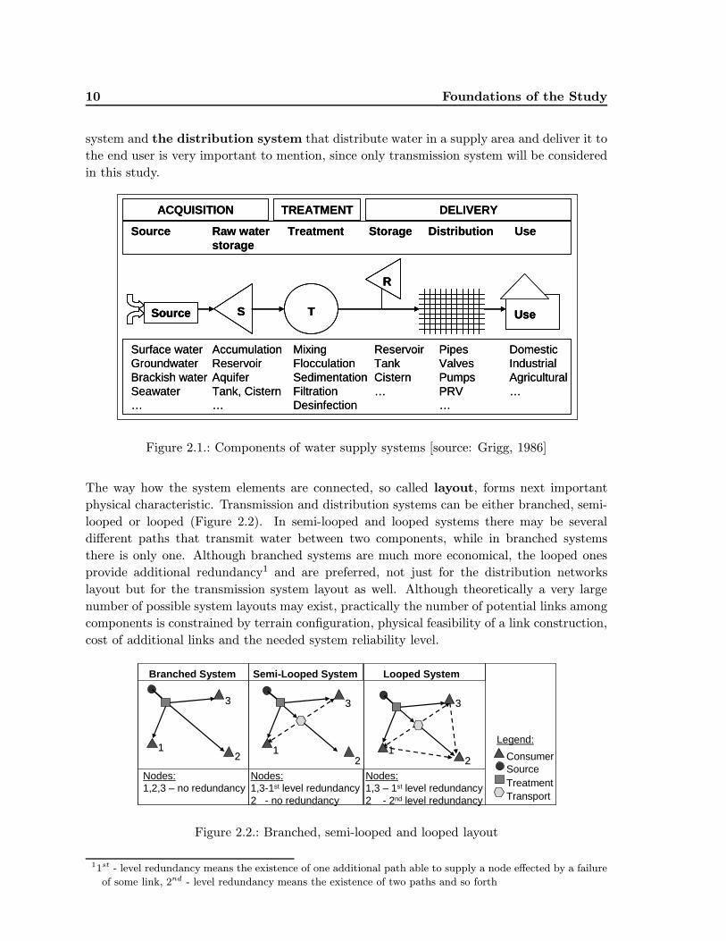
10 Foundations of the Study
system and the distribution system that distribute water in a supply area and deliver it to
the end user is very important to mention, since only transmission system will be considered
in this study.
ACQUISITION
Source
TREATMENT DELIVERY
Raw waterstorage
Treatment Storage Distribution Use
SSource T
R
Use
Surface waterGroundwaterBrackish waterSeawater…
AccumulationReservoirAquiferTank, Cistern…
MixingFlocculationSedimentationFiltrationDesinfection
ReservoirTankCistern…
PipesValvesPumpsPRV…
DomesticIndustrialAgricultural…
ACQUISITION
Source
TREATMENT DELIVERY
Raw waterstorage
Treatment Storage Distribution Use
SSource T
R
UseSSource T
R
Use
Surface waterGroundwaterBrackish waterSeawater…
AccumulationReservoirAquiferTank, Cistern…
MixingFlocculationSedimentationFiltrationDesinfection
ReservoirTankCistern…
PipesValvesPumpsPRV…
DomesticIndustrialAgricultural…
Figure 2.1.: Components of water supply systems [source: Grigg, 1986]
The way how the system elements are connected, so called layout, forms next important
physical characteristic. Transmission and distribution systems can be either branched, semi-
looped or looped (Figure 2.2). In semi-looped and looped systems there may be several
different paths that transmit water between two components, while in branched systems
there is only one. Although branched systems are much more economical, the looped ones
provide additional redundancy1 and are preferred, not just for the distribution networks
layout but for the transmission system layout as well. Although theoretically a very large
number of possible system layouts may exist, practically the number of potential links among
components is constrained by terrain configuration, physical feasibility of a link construction,
cost of additional links and the needed system reliability level.
1122
33
1122
33
1122
33
Nodes:1,2,3 – no redundancy
Nodes:1,3-1st level redundancy2 - no redundancy
Nodes:1,3 – 1st level redundancy2 - 2nd level redundancy
Branched System Semi-Looped System Looped System
ConsumerSourceTreatmentTransport
Legend:11
22
33
1122
33
1122
33
Nodes:1,2,3 – no redundancy
Nodes:1,3-1st level redundancy2 - no redundancy
Nodes:1,3 – 1st level redundancy2 - 2nd level redundancy
Branched System Semi-Looped System Looped System
ConsumerSourceTreatmentTransport
Legend:
Figure 2.2.: Branched, semi-looped and looped layout
11st - level redundancy means the existence of one additional path able to supply a node effected by a failure
of some link, 2nd - level redundancy means the existence of two paths and so forth
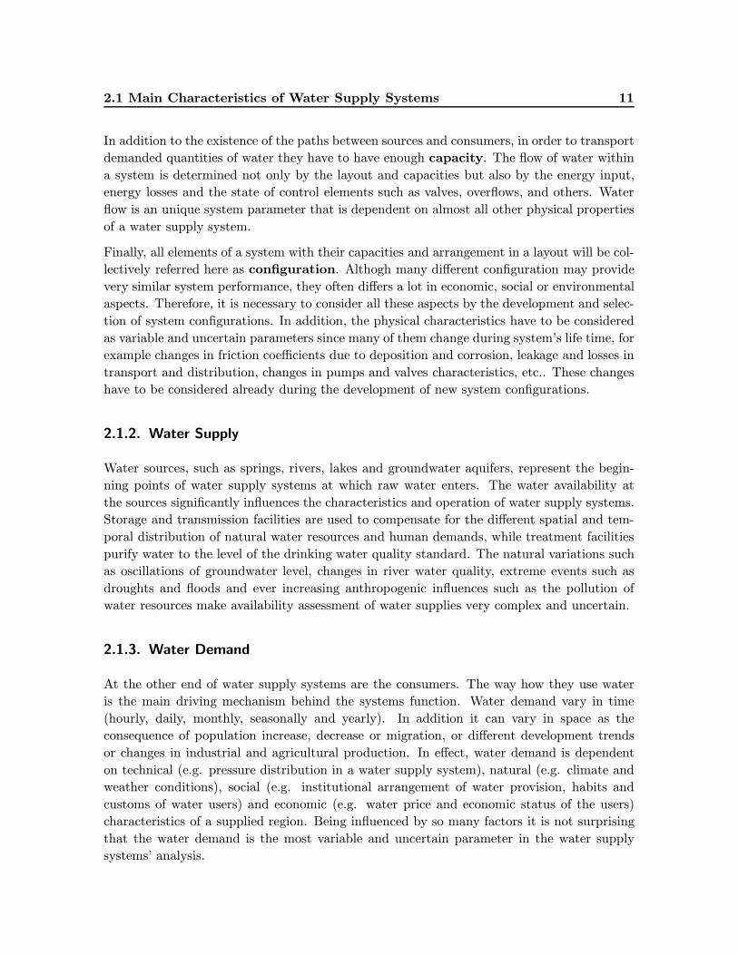
2.1 Main Characteristics of Water Supply Systems 11
In addition to the existence of the paths between sources and consumers, in order to transport
demanded quantities of water they have to have enough capacity. The flow of water within
a system is determined not only by the layout and capacities but also by the energy input,
energy losses and the state of control elements such as valves, overflows, and others. Water
flow is an unique system parameter that is dependent on almost all other physical properties
of a water supply system.
Finally, all elements of a system with their capacities and arrangement in a layout will be col-
lectively referred here as configuration. Althogh many different configuration may provide
very similar system performance, they often differs a lot in economic, social or environmental
aspects. Therefore, it is necessary to consider all these aspects by the development and selec-
tion of system configurations. In addition, the physical characteristics have to be considered
as variable and uncertain parameters since many of them change during system’s life time, for
example changes in friction coefficients due to deposition and corrosion, leakage and losses in
transport and distribution, changes in pumps and valves characteristics, etc.. These changes
have to be considered already during the development of new system configurations.
2.1.2. Water Supply
Water sources, such as springs, rivers, lakes and groundwater aquifers, represent the begin-
ning points of water supply systems at which raw water enters. The water availability at
the sources significantly influences the characteristics and operation of water supply systems.
Storage and transmission facilities are used to compensate for the different spatial and tem-
poral distribution of natural water resources and human demands, while treatment facilities
purify water to the level of the drinking water quality standard. The natural variations such
as oscillations of groundwater level, changes in river water quality, extreme events such as
droughts and floods and ever increasing anthropogenic influences such as the pollution of
water resources make availability assessment of water supplies very complex and uncertain.
2.1.3. Water Demand
At the other end of water supply systems are the consumers. The way how they use water
is the main driving mechanism behind the systems function. Water demand vary in time
(hourly, daily, monthly, seasonally and yearly). In addition it can vary in space as the
consequence of population increase, decrease or migration, or different development trends
or changes in industrial and agricultural production. In effect, water demand is dependent
on technical (e.g. pressure distribution in a water supply system), natural (e.g. climate and
weather conditions), social (e.g. institutional arrangement of water provision, habits and
customs of water users) and economic (e.g. water price and economic status of the users)
characteristics of a supplied region. Being influenced by so many factors it is not surprising
that the water demand is the most variable and uncertain parameter in the water supply
systems’ analysis.
12 Foundations of the Study
2.1.4. System Performance Measures
Present water supply systems range form small scale systems with a single source, no treat-
ment and simple transport system to large regional systems which comprise numerous ground
and surface sources, treat water at complex treatment facilities and deliver it to large dis-
tribution networks that consists of many reservoirs and pump stations, thousands of pipes
and pipe fittings, various controllers and measurement devices and have very sophisticated
operation and management systems. Although numerous performance measures are of im-
portance for the functioning of such complex systems, from the technical point of view, the
two most determining ones are water flows and pressures. They represent the essence of any
quantitative analysis of water supply systems and will be adopted as the main indicators of
a system’s performance.
2.2. Environmental and Socioeconomic Issues of Importance
Until the last decade, aside from rare examples such as a three volume series on the social and
environmental effects of large dams of Goldsmith and Hildyard (1984, 1986, 1992) and the
revision of large water project impacts on low-income rural communities in subtropical and
tropical river basins of Biswas (1996), there were not many attempts to quantify impacts of
water supply systems on the society (for overview see Scudder, 1996; Chadwick, 2002). Such
a need emerged only when the degraded state of the environmental quality threaten to either
directly or indirectly endanger the human’s health and the future prosper of our society. To-
day there is an increasingly large number of literature about negative environmental impacts
of large scale water projects. Some large scale examples of the depletion of natural water
sources, such as the Ogallala aquifer in the USA (Wilhite, 1988), the Yellow river in China
(Zhu et al., 2004) or the Caspian, Aral and Dead seas (Kobori and Glantz, 1998) in Eurasian
region, and thousands other smaller examples of the pollution of water ecosystems, led to the
development of large number of methods for the environmental impacts assessment (EIA).
An overview of these methods can be found in Yurdusev (2002). Essentially each method
consists of two basic steps: a) identification of impacts and b) their quantification. The same
two steps are adopted for the integration of environmental and socioeconomic issues in the
water supply systems’ analysis.
2.2.1. Environmental Impacts of Water Supply Systems
It is broadly adopted that engineering projects may have impacts on the full range of environ-
mental components, including air, water, land, ecology and noise as well as on the physical
processes that occur in the environment (CIRIA, 1994). Experience suggests that the effects
of large scale projects have to be considered on three time scales: a) during construction,
b) upon completion and c) over the period of exploitation, and on several space scales: a)
immediate surroundings, b) the neighbourhood, and c) wider possibly affected areas (Munn,
2006). In addition, impacts may be directly attributable to the project (e.g. lowering of
the groundwater table due to water withdrawal) or indirectly caused (e.g. land degradation
2.2 Environmental and Socioeconomic Issues of Importance 13
due to the building material excavation). Although environmental impacts of an engineer-
ing project are very site and project specific, the study of Construction Industry Research
and Information Association form England (CIRIA, 1994) provide a good overview of the
possible environmental impacts of water supply systems on air, water, land and ecology (see
appendix A.1). Based on this study, the most common environmental impacts of water supply
projects are summarized in the following.
Air quality in the neighbourhood of a water supply system can be temporarily affected
during the construction by entrainment of dust from aggregate stockpiles and haulage roads
or permanently affected by changing the micro-climate around accumulations such as raw
water storages. Furthermore, such open water surfaces increase evapotranspiration rates
that may influence the vegetation in the area or increase the frequency of fog and mists. The
potential impacts are usually assessed by calculating the water balance with and without
accumulation.
Abstractions from groundwater aquifers and rivers reduce thewater amount available in these
systems and in extreme cases may lead to the depletion of aquifers, the loss of river base flow
and the devastation of wetlands and other ecosystems. Furthermore, reduced water quantity
in natural systems influence its quality and promote development of higher concentration of
pollutants and nutrients. In addition, river impoundments and water supply accumulations
may influence not just river flow regime but may also rise the groundwater table and influence
the interactions among surface and groundwater bodies. Application of standard hydrological
and hydrogeological methods for the balancing of the water resources is the most often used
way to determine the allowable water withdrawal quantities.
Building of accumulations and objects as well as installation of pipelines, cause the loss of
land resources and may impact ecological sites and the open space amenity value. Large water
impoundments and accumulations may, in addition, cause slope failures or increase pressure
in geological fault zones. In contrast, water supply intake places are usually protected by
zones of reduced human activity in which the natural state of the resources is protected.
Water accumulations cause not just permanent loss of flooded habitats but significantly im-
pact upstream and downstream geomorphological processes and habitat conditions. Decrease
or increase of river velocity may favour some species at the expense of others and physical
barriers and loss of high flows may cease the migration of some fish species. Reduction in
available groundwater and river water amounts and reduction of their natural variations,
may lead to changes in the ecology of river corridors, estuaries and wetlands. Habitat and
ecological studies may to some extent assess these changes.
2.2.2. Quantification of Environmental Costs and Benefits
In order to avoid the above stated negative environmental impacts it is necessary to assess
the state of an ecosystems prior to a project and assess the possible changes that may be
caused by a project. Furthermore, in order to be able to make a comparison among project
alternatives and to make trade-off with other project objectives a quantitative or qualitative
categorization of the value of the environment has to be made. Since this is not an easy task,
14 Foundations of the Study
the environmental impacts of a project or an action are often expressed through indicators 2.
A very complete list of environmental indicators of importance in relation to water resources
projects has been published by UNESCO (1987). But the quantification of the impacts of
a project even using indicators is still a very complex problem. While some environmental
indicators, for example the decrease in a groundwater level, are quantifiable or measurable,
others such as recreational or aesthetic value of the environment, can be only qualitatively
expressed. In order to overcome such differences some EIA methods use qualitative eval-
uation for all indicators (i.e. ad hoc, checklist or overlay methods), some avoid expressive
quantification by establishing direct dependencies among project activities and environmen-
tal indicators (i.e. Matrices and Network technologies) while some transform all impacts to
monetary terms (i.e. Benefit-cost analysis). The first group is often judged as too rough and
vague since it a) evaluates indicators mainly by auditing experts, decision makers and other
parties of interests that express their subjective opinion and b) because it uses qualitative
values, such as ”good” and ”bad” that may have different meanings for different participating
parties. Placing a monetary value on environmental impacts is based on the assumption that
individuals are willing to pay for environmental gains or, conversely, are willing to accept
compensation for some environmental losses. Such techniques are not just subjective to the
individual preferences (Pearce and Markandya, 1993) but one has to keep in mind that the
willingness to pay or the willingness to accept should reflect the preferences of future genera-
tions and other species and are extremely difficult to forecast (Beder, 2002). In addition, the
market value might not be consistent with long-term welfare or survival of society, since the
economy is interested in the environment only to the extent that it can ensure a continuous
supply of goods and services to meet human wants (Beder, 2002). Finally, the approach based
on the establishment of the direct dependencies among project activities and environmental
indicators is selected as the most appropriate.
The assessment of changes of some environmental indicator as a consequence of some projects
or actions is a very complex task that often requests complex studies. Stated that the
enclosure of a broad range of functional relationships between water supply project properties
(e.g. withdrawal rates, transported quantities, etc.) and their environmental impacts (e.g.
groundwater level, river water flow, etc.) within one systematic framework is the prime
focus of this study, instead of the development of the models for the assessment of individual
impact it is assumed that the dependencies of the indicators states from the project properties
or some project actions can be represented as simple single-variable functional relationships.
Since these relationships are to be used for the selection among alternative project parameters
or actions, they do not need to represent the environmental impacts in absolute values but
can only represent the relative difference among different project parameter values or actions.
Similar as the other engineering parameters, such as expected water demands or estimated
operation costs, the environmental impacts may be approximated by: a) statistical evaluation
of existing data, if available, b) transferring of the results from similar studies, c) using
existing knowledge about natural processes (e.g. impacts of the lowering of a groundwater
level on the surface vegetation or decreased river flows on fish species) or d) different kinds
of trends analysis and logical deduction. In addition it is argued that a simplified functional
relationships between environmental impacts and project parameters may have the accuracy
2numbers or ratios that help to reveal the status and changes of selected parameters
2.2 Environmental and Socioeconomic Issues of Importance 15
of the similar order of magnitude as most other input parameters (e.g. prediction of vegetation
cover reduction upon decrease in groundwater level has a similar order of accuracy as the
prediction of economic costs of installation and operation of pump station in some future time
period) and that the approximate but systematic evaluation of a broad range of environmental
effects may be much more beneficial than a more precise analysis that is focused on few
impacts only. Furthermore, the accuracy of the EIA is dependent on the stage in water supply
management it serves for. While for the planning phase the general trends and tendencies
may be enough to identify the most sensitive environmental areas that is to be preserved,
the design and operation phase will need much more accurate functional relationships among
environmental indicators and parameters of a system. But in these phases much more data,
time and resources may be available for the EIA and the functional dependencies can be
much better accommodated to a particular site or even detailed simulation models may be
developed.
2.2.3. Socioeconomic Aspects of Water Supply Systems
The social impacts analysis can be defined as an analysis of project impacts on sociocultural
systems (SCOPE, 1972). Beside obvious benefits, such as improved hygienic-health condi-
tions and better living standards, water supply projects may cause non-desirable migrations
of population toward places where the systems have been built, loss of populations primary
activities or the changes in population habits and customs. In addition, under the circum-
stance of good water availability a trend for the not-beneficial water use and its dissipation
often develops (e.g. cars and street washing). Although some general dependencies between
water provision and its social impacts may be reasonably assumed (e.g. provision of water
attracts new population) the assessment of the more detailed social impacts is almost an im-
possible task. Furthermore, for most types of the engineering analysis much more important
social aspects are the preferences of the investors, public or authorities that are not the con-
sequence of a project or actions but are input parameters to the analysis. These preferences
are often the determining factor in the ”choice” between project alternatives and have to be
considered within the integrated decision support.
Water supply systems provide support for many important economic activities such as the
agriculture, livestock and many other industries. Furthermore, the economic aspects, such
as the economic benefits of water provision or the investment and operation costs of the
systems elements are still the main decision criteria in planning, designing and operation
of water supply systems. In contrary to other aspects, economic costs and benefits can be
assessed for each alternative systems configuration or management option in monetary units.
Even more, the economic analysis methods, such as Present-worth, Rate-of-Return, Annual-
cost and Benefit-Cost Ratio methods (James and Lee, 1971), allow for the scaling of different
costs in time scale and enable their mutual comparison.
A state’s institutional organization, its form of government, laws and customs constitute
the framework within which society functions and directly effects the water resources ma-
nagement. Although different forms of water supply companies may provide water within a
country, in most cases water supply undertakings come under extensive governmental control
16 Foundations of the Study
exercised through legislation, regulations, standards and inspection procedures. These effect
the objectives, methodological approaches, financial capabilities and operation standards of
water supply providers but are extremely hard to assess and quantify and will not be further
considered in this study. .
The financing of water supply infrastructure, especially of large scale projects, was tradi-
tionally a task carried out by the public sector through forms such as direct investments,
subsidizing, crediting, and others. Although in most of the world countries the provision of
water is still a public responsibility, in the last decades, there is an increasing involvement
of the private sector through various forms of management agreements, lease agreements,
concession or full or partial privatization. The form of ownership and financing may largely
influence the selection of criteria and decision alternatives in management of water supply
but are also extremely hard to quantify and will not be further considered in this study.
Nevertheless the inclusion of the preferences of decision makers in the alternative selection
process allows to incorporate to some extent the institutional and financing aspects.
2.2.4. Quantification of Socioeconomic Costs and Benefits
The way of managing, investing in and thinking about water resource projects is a consequence
of complex social processes such political conditions, social preferences, trends in science
and many others that are constantly taking place in the society. In addition, technological
improvements such as the development of water saving appliances, changes in social norms
such as the increased environmental awareness and global changes such as climate change,
may significantly influence not only the water demand but also the social benefits of water use.
Some of these primary effects can be directly connected to the parameters of the water supply
systems while most of the secondary effects such as the provision of new jobs, resettlement
of population, migration to the urban areas are to case specific to be generalized in the
functional relationships.
Economic benefits of water supply systems are usually assessed based on the economic value
of used water, often referred as willingness to pay, and are either calculated directly analysing
the economic process or by covering from the loss functions of water shortages (e.g. the value
of water used in the food industry may be much greater that the one of water used for cooling
purposes since in the second case water may be easily replaced with some other liquid or by
using recirculating techniques). As far as economic costs are concerned two main types of
costs are of a prime concern: capital (fixed) and operation (variable) costs. For each potential
water supply systems component, these cost can be calculated from the characteristic of the
components (e.g. dimensions, capacities, etc.), conditions of installation or operation (e.g.
terrain, climate, etc.), prices of material, machinery and labour, and economic and financial
conditions, such as availability of credits, rates of interests, and others. Since this is a very
cumbersome process, costs are often approximated with cost coefficients (fixed costs per unit
dimension of a component) or cost functions (functional dependency of costs and size of a
component) that are obtained either by statistically analysing costs of already built systems
or analysing current prices at the market.
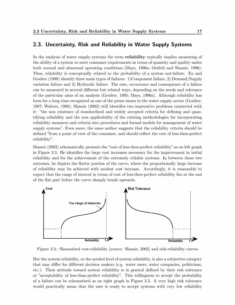
2.3 Uncertainty, Risk and Reliability in Water Supply Systems 17
2.3. Uncertainty, Risk and Reliability in Water Supply Systems
In the analysis of water supply systems the term reliability typically implies measuring of
the ability of a system to meet consumer requirements in terms of quantity and quality under
both normal and abnormal operating conditions (Mays, 1996a; Ostfeld and Shamir, 1996).
Thus, reliability is conceptually related to the probability of a system not-failure. Xu and
Goulter (1999) identify three main types of failures: 1)Component failure, 2) Demand/Supply
variation failure and 3) Hydraulic failure. The rate, occurrence and consequence of a failure
can be measured in several different but related ways, depending on the needs and relevance
of the particular aims of an analysis (Goulter, 1995; Mays, 1996a). Although reliability has
been for a long time recognized as one of the prime issues in the water supply sector (Goulter,
1987; Walters, 1988), Shamir (2002) still identifies two imperative problems connected with
it: ”the non existence of standardized and widely accepted criteria for defining and quan-
tifying reliability and the non applicability of the existing methodologies for incorporating
reliability measures and criteria into procedures and formal models for management of water
supply systems”. Even more, the same author suggests that the reliability criteria should be
defined ”from a point of view of the consumer, and should reflect the cost of less-then-perfect
reliability”.
Shamir (2002) schematically presents the ”cost of less-then-perfect reliability” as on left graph
in Figure 2.3. He identifies the large cost increases necessary for the improvement in initial
reliability and for the achievement of the extremely reliable systems. In between these two
extremes, he depicts the flatter portion of the curve, where the proportionally large increase
of reliability may be achieved with modest cost increase. Accordingly, it is reasonable to
expect that the range of interest in terms of cost of less-then-perfect reliability lies at the end
of the flat part before the curve sharply bends upwards.
Figure 2.3.: Shematised cost-reliability [source: Shamir, 2002] and risk-reliability curves
But the system reliability, or the needed level of system reliability, is also a subjective category
that may differ for different decision makers (e.g. water users, water companies, politicians,
etc.). Their attitude toward system reliability is in general defined by their risk tolerance
or ”acceptability of less-than-perfect reliability”. This willingness to accept the probability
of a failure can be schematised as on right graph in Figure 2.3. A very high risk tolerance
would practically mean that the user is ready to accept systems with very low reliability
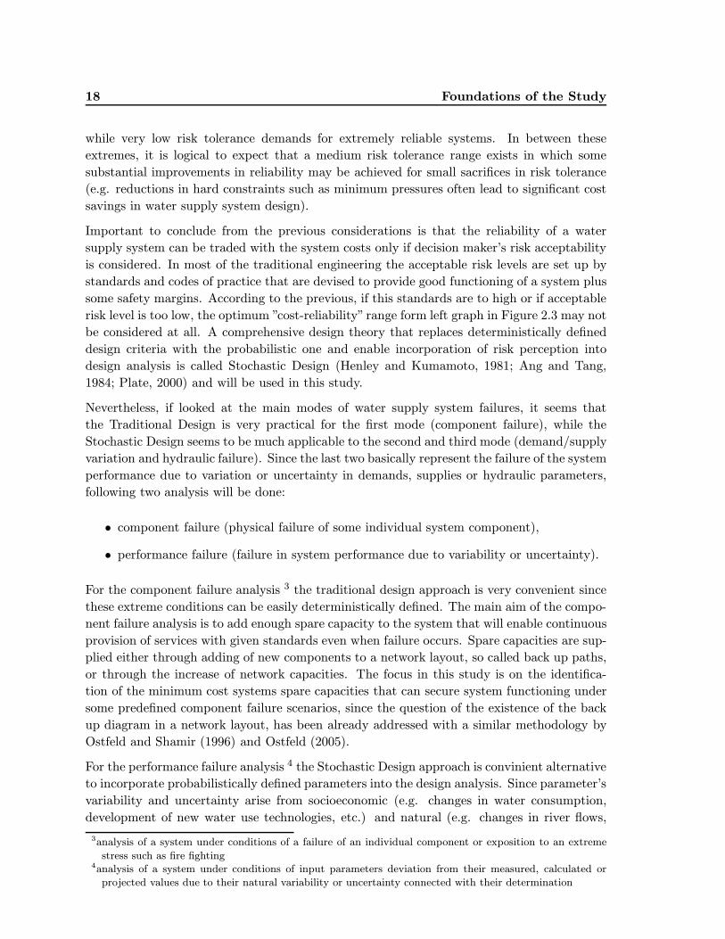
18 Foundations of the Study
while very low risk tolerance demands for extremely reliable systems. In between these
extremes, it is logical to expect that a medium risk tolerance range exists in which some
substantial improvements in reliability may be achieved for small sacrifices in risk tolerance
(e.g. reductions in hard constraints such as minimum pressures often lead to significant cost
savings in water supply system design).
Important to conclude from the previous considerations is that the reliability of a water
supply system can be traded with the system costs only if decision maker’s risk acceptability
is considered. In most of the traditional engineering the acceptable risk levels are set up by
standards and codes of practice that are devised to provide good functioning of a system plus
some safety margins. According to the previous, if this standards are to high or if acceptable
risk level is too low, the optimum ”cost-reliability” range form left graph in Figure 2.3 may not
be considered at all. A comprehensive design theory that replaces deterministically defined
design criteria with the probabilistic one and enable incorporation of risk perception into
design analysis is called Stochastic Design (Henley and Kumamoto, 1981; Ang and Tang,
1984; Plate, 2000) and will be used in this study.
Nevertheless, if looked at the main modes of water supply system failures, it seems that
the Traditional Design is very practical for the first mode (component failure), while the
Stochastic Design seems to be much applicable to the second and third mode (demand/supply
variation and hydraulic failure). Since the last two basically represent the failure of the system
performance due to variation or uncertainty in demands, supplies or hydraulic parameters,
following two analysis will be done:
• component failure (physical failure of some individual system component),
• performance failure (failure in system performance due to variability or uncertainty).
For the component failure analysis 3 the traditional design approach is very convenient since
these extreme conditions can be easily deterministically defined. The main aim of the compo-
nent failure analysis is to add enough spare capacity to the system that will enable continuous
provision of services with given standards even when failure occurs. Spare capacities are sup-
plied either through adding of new components to a network layout, so called back up paths,
or through the increase of network capacities. The focus in this study is on the identifica-
tion of the minimum cost systems spare capacities that can secure system functioning under
some predefined component failure scenarios, since the question of the existence of the back
up diagram in a network layout, has been already addressed with a similar methodology by
Ostfeld and Shamir (1996) and Ostfeld (2005).
For the performance failure analysis 4 the Stochastic Design approach is convinient alternative
to incorporate probabilistically defined parameters into the design analysis. Since parameter’s
variability and uncertainty arise from socioeconomic (e.g. changes in water consumption,
development of new water use technologies, etc.) and natural (e.g. changes in river flows,
3analysis of a system under conditions of a failure of an individual component or exposition to an extreme
stress such as fire fighting4analysis of a system under conditions of input parameters deviation from their measured, calculated or
projected values due to their natural variability or uncertainty connected with their determination
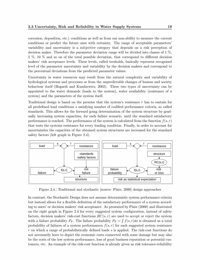
2.3 Uncertainty, Risk and Reliability in Water Supply Systems 19
corrosion, deposition, etc.) conditions as well as from our non-ability to measure the current
conditions or predict the future ones with certainty. The range of acceptable parameters’
variability and uncertainty is a subjective category that depends on a risk perception of
decision maker. Therefore the parameter deviation range will be divided into classes of 1 %,
5 %, 10 % and so on of the total possible deviation, that correspond to different decision
makers’ risk acceptance levels. These levels, called tresholds, basically represent recognised
level of the parameter uncertainty and variability by the decision makers and correspond to
the percentual deviations from the predicted parameter values.
Uncertainty in water resources may result from the natural complexity and variability of
hydrological systems and processes or from the unpredictable changes of human and society
behaviour itself (Bogardi and Kundzewicz, 2002). These two types of uncertainty can be
appointed to the water demands (loads to the system), water availability (resistance of a
system) and the parameters of the system itself.
Traditional design is based on the premise that the system‘s resistance r has to sustain for
all predefined load conditions s satisfying number of codified performance criteria, so called
standards. This allows for the forward going determination of the system structure by grad-
ually increasing system capacities, for each failure scenario, until the standard satisfactory
performance is reached. The performance of the system is calculated from the function f(s, r)
that tests the systems resistance for every loading condition. Finally, in order to account for
uncertainties the capacities of the obtained system structures are increased for the standard
safety factors (left graph in Figure 2.4).
load resistance
failurenot
failure
structure
f(s,r)
-standards-safety factors
s rload resistance
failure probability
riskor loss
risk as statistical expectation
f(s,r)
RC(s,r)
structure
s r
Figure 2.4.: Traditional and stochastic [source: Plate, 2000] design approaches
In contrast, the Stochastic Design does not assume deterministic system performance criteria
but instead allows for a flexible definition of the satisfactory performance of a system accord-
ing to users’ or decision makers’ risk acceptance. As presented by Plate (2000) and illustrated
on the right graph in Figure 2.4 for every suggested system configuration, instead of safety
factors, decision makers’ risk-cost functions RC(s, r) are used to accept or reject the system
with a failure probability PF . The failure probability PF =∫f(s, r)ds is obtained as a total
probability of failures of a system performances f(s, r) for each suggested system resistance
r on which a range of probabilistically defined loads s is applied. The risk-cost functions do
not necessarily have to depict the economic costs connected with some damage but may also
be the costs of the low system performance, loss of good business reputation or potential cus-
tomers, etc. An example of the risk-cost function is already given as risk tolerance-reliability
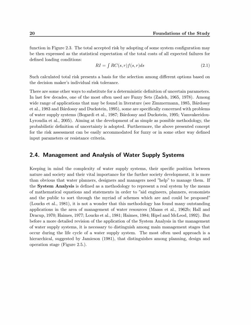
20 Foundations of the Study
function in Figure 2.3. The total accepted risk by adopting of some system configuration may
be then expressed as the statistical expectation of the total costs of all expected failures for
defined loading conditions:
RI =∫RC(s, r)f(s, r)ds (2.1)
Such calculated total risk presents a basis for the selection among different options based on
the decision maker’s individual risk tolerance.
There are some other ways to substitute for a deterministic definition of uncertain parameters.
In last few decades, one of the most often used are Fuzzy Sets (Zadeh, 1965, 1978). Among
wide range of applications that may be found in literature (see Zimmermann, 1985, Bardossy
et al., 1983 and Bardossy and Duckstein, 1995), some are specifically concerned with problems
of water supply systems (Bogardi et al., 1987; Bardossy and Duckstein, 1995; Vamvakeridou-
Lyroudia et al., 2005). Aiming at the development of as simple as possible methodology, the
probabilistic definition of uncertainty is adopted. Furthermore, the above presented concept
for the risk assessment can be easily accommodated for fuzzy or in some other way defined
input parameters or resistance criteria.
2.4. Management and Analysis of Water Supply Systems
Keeping in mind the complexity of water supply systems, their specific position between
nature and society and their vital importance for the further society development, it is more
than obvious that water planners, designers and managers need ”help” to manage them. If
the System Analysis is defined as a methodology to represent a real system by the means
of mathematical equations and statements in order to ”aid engineers, planners, economists
and the public to sort through the myriad of schemes which are and could be proposed”
(Loucks et al., 1981), it is not a wonder that this methodology has found many outstanding
applications in the area of management of water resources (Maass et al., 1962b; Hall and
Dracup, 1970; Haimes, 1977; Loucks et al., 1981; Haimes, 1984; Hipel and McLeod, 1992). But
before a more detailed revision of the application of the System Analysis in the management
of water supply systems, it is necessary to distinguish among main management stages that
occur during the life cycle of a water supply system. The most often used approach is a
hierarchical, suggested by Jamieson (1981), that distinguishes among planning, design and
operation stage (Figure 2.5.).
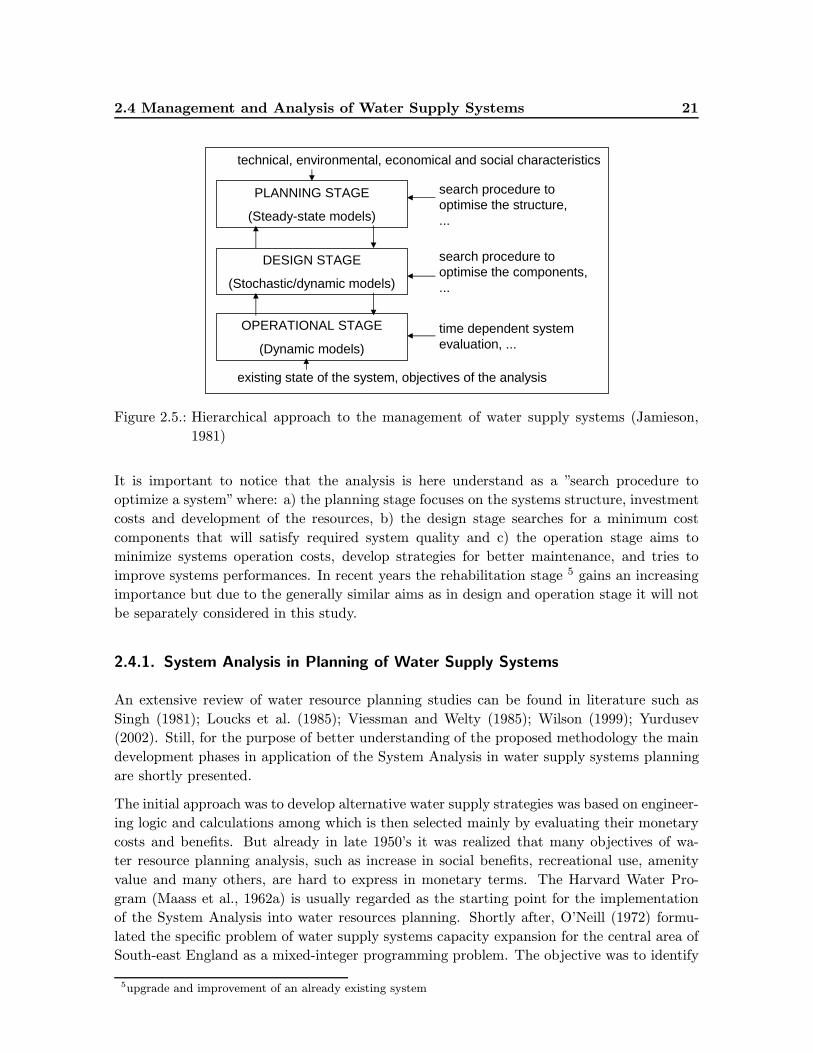
2.4 Management and Analysis of Water Supply Systems 21
PLANNING STAGE
(Steady-state models)
DESIGN STAGE
(Stochastic/dynamic models)
OPERATIONAL STAGE
(Dynamic models)
technical, environmental, economical and social characteristics
search procedure to optimise the structure, ...
search procedure to optimise the components, ...
time dependent system evaluation, ...
existing state of the system, objectives of the analysis
Figure 2.5.: Hierarchical approach to the management of water supply systems (Jamieson,
1981)
It is important to notice that the analysis is here understand as a ”search procedure to
optimize a system”where: a) the planning stage focuses on the systems structure, investment
costs and development of the resources, b) the design stage searches for a minimum cost
components that will satisfy required system quality and c) the operation stage aims to
minimize systems operation costs, develop strategies for better maintenance, and tries to
improve systems performances. In recent years the rehabilitation stage 5 gains an increasing
importance but due to the generally similar aims as in design and operation stage it will not
be separately considered in this study.
2.4.1. System Analysis in Planning of Water Supply Systems
An extensive review of water resource planning studies can be found in literature such as
Singh (1981); Loucks et al. (1985); Viessman and Welty (1985); Wilson (1999); Yurdusev
(2002). Still, for the purpose of better understanding of the proposed methodology the main
development phases in application of the System Analysis in water supply systems planning
are shortly presented.
The initial approach was to develop alternative water supply strategies was based on engineer-
ing logic and calculations among which is then selected mainly by evaluating their monetary
costs and benefits. But already in late 1950’s it was realized that many objectives of wa-
ter resource planning analysis, such as increase in social benefits, recreational use, amenity
value and many others, are hard to express in monetary terms. The Harvard Water Pro-
gram (Maass et al., 1962a) is usually regarded as the starting point for the implementation
of the System Analysis into water resources planning. Shortly after, O’Neill (1972) formu-
lated the specific problem of water supply systems capacity expansion for the central area of
South-east England as a mixed-integer programming problem. The objective was to identify
5upgrade and improvement of an already existing system
22 Foundations of the Study
the minimum cost capital and operation development scenario by transferring the water re-
sources from different potential sources with pre-specified yields to the demand centres with
predefined marginal demands. At about the same time Butcher et al. (1969) used a dynamic
programming model to determine the ”optimal” construction sequence of additional system
capacity to meet increasing demand. This model used the cost per unit supply available from
each water source to differentiate among sources and was able to account for the effects of
interest rate. Later on, it was modified by Esogbue and Morin (1971) to allow more general
selection and sequencing of available expansion capacities.
Once set up as a minimum cost optimization problem, various system analysis techniques
found their way in the planning studies of water supply systems. One of the most cited stud-
ies is the North Atlantic Regional Water Resource Study (Haimes, 1977; Cohon, 1978) that
used the Linear Programming technique to allocate available resources to water demands.
Since the Linear Programming is applicable only to problems that have linear dependencies
among parameters, in 1980’s various other mathematical programming techniques have been
tried. de Monsabert et al. (1982) and Gorelick et al. (1984) tried with the Non-linear Pro-
gramming but as identified by McKinney and Lin (1994) this technique is not able to handle
interdependency among parameters and may have difficulties in determination of the gradi-
ents for highly non-linear dependencies. The Goal Programming technique, such as in Rajabi
et al. (1999), suffered from often too large sets of possible system states and is therefore more
convenient for nested problems with sequential decisions (Vink and Schot, 2002). These as
well as many other techniques, based on the evaluation of gradients, tend to end up in lo-
cal optima and are not convenient for discrete problems with many near optimal solutions
(Dandy et al., 1996b).
In 1990’s it has become clear that the exact mathematical programming techniques are com-
putationally too demanding for complex optimization problems, and approximate techniques
come into the play. Among them the Genetic Algorithms turned out to be the most often used
one. Dandy and Connarty (1995); Dandy et al. (1996b) introduced this approach to project
sizing and scheduling of different dam combinations and sizes while Vink and Schot (2002)
used it for the determination of optimal production strategies from different groundwater
sources. Another often used robust heuristic technique is Simulated Annealing. Ejeta and
Mays (2005) used this approach for development of optimal timing of the capacity expansion
of water supply conveyance and identification of optimal water allocation policy. Although
such models have proved their value for many theoretical problems their application in prac-
tice is still waiting behind. The lack of good conceptual representation of the systems, or the
one that does not coincide with the user conceptualization, may be one of the biggest reasons
for that (Loucks et al., 1985; Walski, 2001).
Already in 1970’s it was recognized that the consideration of only economic criteria does
not suit to the complex multi-objective aims of the water supply planning analysis. Lawson
(1974) tried to upgrade the model of O’Neill (1972) for considering environmental quality
by omitting sources that are environmentally sensitive. Similarly Page (1984) developed an
iterative procedure for allocating water transfers to meet water demands at five-year inter-
vals by constraining of the environmentally sensitive sources. Another example of treating
environmental issues as constraints to the, in this case, Transportation-type Programming
approach is introduced by Stephenson (1982). Several optimization models focused on the
2.4 Management and Analysis of Water Supply Systems 23
incorporation of social trends and preferences into water supply system management. Lund
(1987) used the Sequential Linear Programming method to evaluate and schedule water con-
servation measures that minimize system costs by avoiding or deferring capacity expansion
while Rubenstein and Ortolano (1984) used the Dynamic Programming to design demand
management option that supplements limited available water sources. Among models that
used the Decomposition Approach to address the environmental impacts and socioeconomic
effects together, the Wu (1995) and Kirshen et al. (1995) are among the most famous ones.
Wu (1995) developed a separated module (Regional Model for Impact Assessment) in order to
report on the state of physical quantities and socioeconomic quantities for different alternative
development scenarios. Similarly, Kirshen et al. (1995) coupled modules for the evaluation
of environmental, social and cultural impacts with water allocation among sources, demands
and treatment facilities. This model, as well as some others such as Watkins et al. (2004);
Yamout and El-Fadel (2005) is further developed with the aim to cover a full range of issues
and uncertainties faced by water planners, including those related to climate, watershed con-
dition, anticipated demand, ecosystem needs, regulatory climate, operation objectives and
others. Such complex and sophisticated models are meant for governmental or national level
water resources management and are not providing a practical solution for the planning and
development of a single water supply system. In addition, they demand a very large amount
of data and are quite cumbersome for practical use.
In parallel to the increasing awareness of the importance of environmental and social aspects
in water resources management, a rapid progress in information technologies enabled the use
of “interactive computer programs that utilize analytical methods, such as decision analysis,
optimization algorithms, program scheduling routines, and so on, for developing models to
help decision makers formulate alternatives, analyse their impacts, and interpret and select
appropriate options for implementation” (Adelman, 1992). From this definition it is more
than obvious that such models, often referred as Decision Support Systems (DSS), are a very
complex aggregation of data processing tools (databases, statistical analysis software, etc.),
simulation and optimization models (representation of process and creation of optimal system
alternatives), and expert systems for the evaluation of alternative’s effects and guidance of
decision makers during the evaluation and selection of final plans. Loucks and da Costa
(1991) give an excellent review of the application of DSS prior to the 1990’s while the review
of some of the numerous latter DSS models can be found in: Watkins and McKinney (1995),
Ejeta and Mays (1998), AWRA (2001) and Geertman and Stillwell (2003). As far as the
water supply planning in specific is concerned after development of numerous integrated
ground and surface water bodies and water supply systems simulation-optimization models,
such as in Nishikawa (1998); Belaineh et al. (1999); Srinivasan et al. (1999); Yang et al.
(2000); Ito et al. (2001); Vink and Schot (2002) in recent years the researches focused on the
better integration of primary issues such as water availability (Luketina and Bender, 2002),
water demand (Hopkins et al., 2004) or institutional constraints (Ejeta et al., 2004). As a
consequence there is an evident trend to reduce the complexity of the models in order to
make them more practical and promote their greater use. Although also an agglomeration of
quite a few sub-models, the CALVIN model (Draper et al., 2003) presents a good example
for pragmatical approach in evaluating various benefits and costs of water provision and is
based on very simple benefit and cost functions. In addition the model uses the network
24 Foundations of the Study
representation of water supply systems that makes it more understandable for potential users
and more computationally effective. But the fact that it uses piecewise linear approximation
of the cost and benefit functions theoretically hinders its usefulness for non-linear and concave
problems.
Finally it can be concluded that the need for methods that are, on one side, based on easily
understandable concepts and techniques and, on the other side, able to deal with complex
multi-objective water supply planning problems still exists. Furthermore the need for the in-
tegration of economic, environmental and social objectives in the development of water supply
strategies and the necessity for the transparent creation of a broad range of alternative water
supply planning options in order to better support multi-objective decision making, are iden-
tified as the main priorities of the future research. The development of the methodology that
is based on some simple mathematical representation and is able to integrate main technical,
environmental and socioeconomic aspects of importance into one unique framework for the
identification of the multi-objective water supply planning options, is the main attention of
this study.
2.4.2. System Analysis in Design of Water Supply Systems
Since 1960’s the optimization of water distribution networks has been one of the most heavily
researched areas. Very comprehensive reviews can be found in: Walski (1985b); Goulter
(1987); Walters (1988); Subramanian (1999); Lansey (2000). In 1980’s Walski (1985a) and
Goulter (1987) were predicting that the state-of-the-art optimization models of that time,
will soon find their widespread use in practice. Although these models showed a certain
degree of robustness and proved their capabilities of handling relatively complicated design
problems in the famous ”Battle of Network Models” (Walski et al., 1987), one decade later,
the same authors (Goulter, 1992; Walski, 1995) were busy trying to identify the reasons why
such predictions did not came true.
The first models for the water distribution network design (Karmeli et al., 1968; Schaake and
Lai, 1969) were developed for branched networks and even though Swamee et al. (1973) proved
the optimality of branched network for a single demand pattern, networks with no built-in
redundancy were of no interest for practice. Although from an engineering intuitive point of
view, the loops have been already for a long time recognized as a ”best practice”way to bring
redundancy into the system, for the modellers, the loops have brought significant complexity
into the algorithms. While in a branched system a given demand pattern uniquely defines the
flows in the network, in a looped system there is a very large number of flow combinations
that can meet a specified demand pattern (Goulter, 1992). Only in late 1970s the researchers
have managed to solve the distribution network design problem by decomposing it into an
optimization part, which searches for minimum cost design parameters, and a simulation
part that calculates network hydraulic properties for one design configuration (Alperovits
and Shamir, 1977; Bhave, 1978; Quindry et al., 1981; Rowell and Barnes, 1982). As identified
by Templeman (1982), these first looped network designs were ”implicitly branched”. They
were made by cross connecting optimized branched systems and, as noted in the same work, do
need a sufficient number of simulations with different demand patterns or component failure
2.4 Management and Analysis of Water Supply Systems 25
scenarios to increase capacities on all alternative paths. In order to improve the procedure
for finding an optimal solution and better address some inherent system properties such as
redundancy, reliability or uncertainty of input parameters, researchers have tested different
approaches such as deterministic, stochastic, heuristic, entropy based and various types of
their combinations.
One of the most important deterministic network optimization works is the Linear Program-
ming Gradient Method of Alperovits and Shamir (1977), which firstly formulate hydraulic
loops for each source-demand node path and then modify the flow distribution based on the
gradient of total costs with respect to such a change. This method improved by Quindry
et al. (1981) as well as similar formulations based on the Linear Programming techniques
from Lansey and Mays (1985), Fujiwara et al. (1987), and Kessler and Shamir (1989) or
the Sherali and Smith (1993) approach with design capacities as optimization variables in-
stead of flows, suffer of finding only a local optima, since this is an inherent property of
gradient based searches. Moreover, starting with Chiplunkar et al. (1986), many researchers
have tried to use the Non-linear Programming technique but in addition to the local optima
problem (Gupta et al., 1999), as identified by Cunha and Sousa (1999), the conversion of
discrete market available pipe diameters to continuous variable additionally influence slow
convergence of the solution technique. Although such results significantly enforced the use
of stochastic procedures it must be noted that the approach proposed by Eiger et al. (1994)
is often identified as first global solution to the network design problem. This algorithm em-
ploys the Branch and Bound procedure to control the production of an improving sequence
of local solutions, the hydraulic consistency is provided via enumeration of all possible ba-
sic loops and source-demand node paths while the prescribed tolerance between the global
lower bound produced by solving a dual problem and the best funded value define stopping
criteria. Sherali and Smith (1997) used the Tight Linear Programming relaxations in order
to compute lower bound and also embedded their Reformulation-Linearisation technique in a
Branch and Bound scheme. Although these algorithms and some of their later improvements
(Sherali et al., 1998, 2001) solved some of the test problems for network design to the global
optimality the computational demands and models complexity were still too high to be used
by practitioners.
Being a non-convex problem with discrete decision variables and a large number of local op-
tima, the network design problem has been in recent years frequently addressed by stochastic
and heuristic optimization techniques. The stochastic procedures are mainly used to address
the uncertainty of the input parameters and heuristic procedures to advance the optimiza-
tion process. Capability of simultaneous dealing with a set of discrete points from decision
variable space, flexible formulation of objective functions and ease to escape local optima
present some of the main advantages of heuristic methods. These methods are very com-
putationally demanding and the randomness of the funded solution give no possibility to
prove whether it is a true global optimum or not. The Genetic Algorithms have been the
most often used heuristic optimization technique (Simpson et al., 1994; Dandy et al., 1996a;
Savic and Walters, 1997; Abebe and Solomatine, 1998; Kapelan, 2003; Tolson et al., 2004;
Babayan et al., 2004; Prasad and Park, 2004; Farmani et al., 2005; Giustolisi and Mastror-
illi, 2005), but the Simulated Annealing (Loganathan et al., 1995; Cunha and Sousa, 1999),
the Ant Colony Optimization (Maier et al., 2003), the Shuffled Frog Leaping (Eusuff and
26 Foundations of the Study
Lansey, 2003), the Shuffled Complex Evolution (Liong and Atiquzzaman, 2004) and others
have been used as well. Giustolisi and Mastrorilli (2005) integrated the Genetic Algorithm
optimization technique with variance reduction Monte Carlo sampling technique, called the
Latin Hypercube, to allow fast identification of a set of near optimal solutions with accu-
rate sampling of probability functions related to the uncertainty of the design conditions.
Although these optimisation techniques showed excellent performances in solution of many
very complex theoretical water supply design studies, many of them are still too complex for
an average engineering level of knowledge to be more often applicable in practice.
Having identified effective and robust optimization routines for the minimum cost network
design problem, the researchers have realized that, in practice, ”the optimal design of a water
distribution network is a complex multiple objective process involving trade-off between the
cost of the network and its reliability” (Xu and Goulter, 1999). In middle 1990’s, Goulter
(1995) and Mays (1996a) have provided the most comprehensive review of the reliability
analysis works and have stated that the reliability issue is one of the most challenging in
the field of water supply engineering. Two decades later it is still an open research area and
tempts for new solutions.
From the point of view of the component failure analysis (failure of individual system compo-
nents) already Rowell and Barnes (1982) develop a procedure to interconnect pipes in order
to maintain the required level of services. Later on Goulter and Morgan (1983) incorporated
a feedback mechanism and even expanded it with a heuristic search procedure (Morgan and
Goulter, 1985). Lansey and Mays (1989) further advanced this procedure to enable simu-
lation of multiple loading conditions. Many other works from the field of the component
failure analysis have been based on the Path Enumeration Methods (Tung, 1996a) among
which the Cut-set Analysis 6 and the Tie-set Analysis 7 are the most often used ones. Shamir
and Howard (1985); Morgan and Goulter (1985); Tung (1985); Goulter and Coals (1986);
Shamsi and Quimpo (1988); Mays (1989a); Bouchart et al. (1989) used these techniques but
as identified by Khomsi et al. (1996) their applicability to water networks is rather limited.
Firstly due to the quite unrealistic condition that all pipes in a minimum cut set would be
in a failure state at the same time, secondly due to the extensive computation needed for the
identification of all minimum cut sets and thirdly due to the fact that the use of the basic cut
set methods do not incorporate any of the hydraulic conditions which may govern the flow
in a network (the supply to a node may fail completely due to pressure insufficiency without
being entirely isolate by broken pipes). The authors themselves use a simple stochastic model
to simulate pipe breakages and insufficient pipe capacities but not for a pre-processing and
evaluation of demands uncertainty but for a post-processing in order to test the reliability of
a water supply system.
For further development of the component failure analysis the terms: reachability 8 and
connectivity 9 defined by Wagner et al. (1986, 1988a,b) were of crucial importance. These
terms come from the Conditional Probability Reliability Procedures (Tung, 1996a) and many
6set of system components or modes of operation which, when failed, cause failure of the system7set of system components arranged in series which, fails when any of its components or modes of operation
fail8probability that a given demand point is connected to at least one source9probability that all demand points are connected to at least one source
2.4 Management and Analysis of Water Supply Systems 27
researchers used them together with the Minimum Cut-set methods (Su et al., 1987; Quimpo
and Shamsi, 1987, 1991). Although the latter was significantly improved by Quimpo and Wu
(1997) to include hydraulic measures and capacities in the reliability measure, by Yang et al.
(1996) to simplify the algorithm and by Shinstine et al. (2002) to implement the repair-ability
of the components, the Minimum Cut-set approach still suffer from large computational de-
mand needed to calculate path sets for each component or component states combination.
Kessler et al. (1990) developed a much less computational demanding methodology, which
even ensures a certain degree of redundancy, and extended it later together with Ormsbee
and Kessler (1990) to include capacity constraints. Still due to the superficial interpreta-
tions that have not been adequately packaged for practical system-design environments these
methodologies have been underutilized (Beecher et al., 1996).
Lansey et al. (1989) were the first to address the uncertainty in demands and they used a
chance-constrained model to add demand uncertainties upon pressure and pipe roughness co-
efficient uncertainties. Bao and Mays (1990) used the Monte Carlo Simulation for the same
purpose while Duan et al. (1990) used the Continuous-time Markov process to model the avail-
able capacity of pump stations. Many other works in demand variation and hydraulic failure
analysis used probability theory or stochastic simulation to define, or constrain, uncertainty in
demands and hydraulic network performances. These works ranged from simple analysis such
as: supply demand quantities (Beim and Hobbs, 1988; Hobbs and Beim, 1988; Duan et al.,
1990) and use of ratio of expected maximum total demand to total water demanded (Fujiwara
and De Silva, 1990; Fujiwara and Tung, 1991), over use of the chance-constrained network
design for limiting the shortages at nodes in comparison to demand values (Tung, 1985; Park
and Liebman, 1993), use of assumed theoretical probability distribution functions of nodal
demands and pipe roughness (Xu and Goulter, 1998, 1999), use of the First-order Reliability
methods to assess the demands probabilities (Goulter and Coals, 1986; Goulter and Bouchart,
1990; Tolson et al., 2004), reformulation of the stochastic problem as the deterministic one
using standard deviation as measure of the variability of demands (Babayan et al., 2003),
to the representation the nodal demands as fuzzy numbers (Bhave and Gupta, 2004). In its
analysis of the previous research Goulter (1992) identifies the work of Bouchart and Goulter
(1991) as an interesting example of joint consideration of two failure modes (component and
demand variation failure) but still states general difficulty of considering both phenomena
simultaneously and disparity among models which are computationally suitable for inclusion
in optimization frameworks and the ones with good network performance. This may well be
the reason while in most of these models the network performance and optimization are still
decomposed.
Another line of thought explored the concept of entropy, introduced by Templeman (1997), to
assign most likely flows to alternative paths and incorporate redundancy in the optimization
of water distribution systems (Awumah et al., 1990, 1991, 1992). Tanyimboh and Templeman
(1993) suggested that flexible networks can be achieved through maximizing the entropy of
flows and significantly reduced computational time by using estimates obtained by averaging
the upper and lower bounds on reliability (Tanyimboh et al., 1997). Tanyimboh and Sheahan
(2002) proposed the idea of minimum cost maximum entropy designs to identify good layouts
of water distribution systems. Still the relationship between entropy and reliability has yet
to be properly established.
28 Foundations of the Study
Finally it is not to be forgotten that network reliability is in fact defined, or more specifically
constrained, by the fundamental layout of a network (Goulter, 1987). At the same time,
the shape of a network significantly effects the costs and improvements in reliability tend to
degrade the minimum cost objective. In order to address the question of the network layout,
the Graph Theory has been almost exclusively used. Furthermore, the connectivity and
reachability of Wagner et al. (1986), were again a very important research milestones. Based
on the Graph Theory, Ormsbee and Kessler (1990) developed an algorithm which identifies
two independent paths to each demand node. Jacobs and Goulter (1989) investigated the use
of a regular graph target (optimal reliability should be provided by an equal number of graph
links or arcs incident on each node) but concluded that such an approach is not applicable
to water supply systems due to the semi-branched structure of water distribution networks
since peripheral nodes need fewer links incident upon them. Diba et al. (1995) presented a
very interesting combination of the Directed Graph algorithm and the Linear Programming
procedure for solving various large-scale water distribution problems. Although this model
is primary developed to assist the planning process it can be further extended for design
purposes. Based on a connectivity analysis of the network’s entire topology, Ostfeld and
Shamir (1996) introduced the concept of backups and recently, Ostfeld (2005) expanded it
to produce the most flexible pair of operation and backup digraphs that yield first-level
system redundancy (if one arc fails, a minimum of one path from at least one source to all
consumers is retained). Although these works provide a very good basis and even propose
some very practicable suggestions for the network layout design, it has to be noted that the
connectivity/topology analysis has been one of the least researched areas in the water supply
system design.
In the end, it is also important to refer to some of the works which specifically address the
issue of multi-objectiveness in water supply system design and importance of the trade-off
between costs and network performances. Already de Neufville (1970) in his cost-effectiveness
analysis promoted the introduction of system specific objectives and alternative levels of
performances rather than application of the Standards for civil engineering systems design.
Furthermore, the same author recognizes the necessity to address the institutional, social and
behavioural issues that may effect, or constrain, the system design. A very good overview of
the application of multi-objective optimization can be found in Van Veldhuizen and Lamont
(2000) and it seems that among many approaches for dealing with more-then-one objectives
and criteria, the Pareto Dominance Criterion (Pareto, 1896) has been the primarily used one
(Dandy et al., 1996a; Savic and Walters, 1997; Kapelan, 2003; Tolson et al., 2004; Babayan
et al., 2004; Farmani et al., 2005; Giustolisi and Mastrorilli, 2005).
As it can be seen from the above, it is very hard to select among numerous offered approaches
and methodologies and although all individual issues have been already treated, one simple
and easily understandable method with clear representation of the system able to comprise
the multi objective nature of the design process and integrate minimum cost solutions with
the reliability issues, such as components failure and parameters’ uncertainty is still to be
found. Exactly the problem of the identification of the design solutions that provide for
the optimal trade-off among system costs and its reliability is the main focus of the design
analysis in this study. Furthermore, the development of the methodology able to encompass
system investment and operation costs defined with various non-convex function and the
2.4 Management and Analysis of Water Supply Systems 29
system reliability assessment based on the component failure and the parameter uncertainty
analysis is expected. Finally an approach that allows for the integration of the decision
makers’ perception of the needed performance and reliability of water supply systems based
on their risk acceptance is adopted instead of the traditional design based on the engineering
standards and codes.
2.4.3. System Analysis in Operation of Water Supply Systems
The two most obvious aims of the water supply systems operation are to control the hydraulic
performance during operation and to minimise the economic expenditures of water supply
provision. Since the economic expenditures are mainly made of operation and maintenance
costs, the minimisation of these two is an imperative since the early times of conventional
water supply systems. Furthermore, if known that even today in the UK for example, the
electricity costs make approximately 10 % of the total operating expenditures of large water
services companies and that the pumps consume more than 70 % out of these costs (Yates
and Weybourne, 2001), then it is not a wonder that the identification of the minimum cost
pumping operation policies is a very active area of research in last three decades. As in many
other areas that needed computer support for the solution of complex and computationaly
demanding problems, the System Analysis found many usefull applications in the water supply
systems operation as well.
A very good overview of the research work in the water supply systems operation until 1993
can be found in Ormsbee and Lansey (1994). The authors define the operation policy (opera-
tion schedule) as the set of rules when a particular pump or group of pumps are to be turned
on or off over a specified period of time and classify until that time available methods on
the basis of their applicability, applied optimization method and nature of resulting policies.
At that time the Linear Programming (Jowitt et al., 1989; Crawley and Dandy, 1993), the
Mixed-integer Linear Programming (Little and McCrodden, 1989), the Dynamic Program-
ming (DeMoyer and Horwitz, 1975; Sterling and Coulbeck, 1975; Sabet and Helweg, 1985;
Zessler and Shamir, 1989; Ormsbee et al., 1989) and the Non-linear Programming (Chase
and Ormsbee, 1989; Lansey and Zhong, 1990; Brion and Mays, 1991) were among the most
often used methods. In addition to the problems with the linearisation of functions such as
pump efficiency, the large computational demands, and the limitation to the smaller systems
all these methods were exclusively searching for the optimisation of the only one objective,
namely electric energy costs.
Lansey and Awumah (1994) directly related the number of times a pump is turned on and
off over a given life cycle with the pump wear and enabled for the addition of the pump
maintenance costs as the second objective that is to be minimised with the optimisation
analysis. Although today the development of durable and high quality pump’s material
makes this dependency as questionable, the recognition of the importance of the inclusion of
multiple objectives in the optimisation of the water supply systems operation significantly
added to the problem complexity and favoured the application of the approximate methods
instead of the analytic ones.
Two applications of the Knowledge-based selection (Fallside, 1988; Lannuzel and Ortolano,
30 Foundations of the Study
1989) that combine a simulation model with a rule based expert optimisation system, provided
some insight into the utility of the Expert System approach. Kansal et al. (2000) continued
this approach and developed an expert system, called EXPLORE, for the management of the
Seville City water supply system that achieve 25 % reduction of the energy costs.
Pezeshk and Helweg (1996) applied the Adaptive Search algorithm and Mackle et al. (1995)
applied the Genetic Algorithm for the optimisation of the pumping electric energy cost.
Savic et al. (1997) proposed a hybridisation of the Genetic Algorithm with a local search
method, in order to include pump maintenance costs and de Schaetzen (1998) included the
system constraints by establishing penalties functions. Baran et al. (2005) proved that the
Evolutionary Computations are a powerful tool to solve optimal pump-scheduling problems
and successfully tested six different Multi-objective Evolutionary Algorithms on a problem
with four objectives: electric energy cost, maintenance cost, maximum power peak and level
variation in a reservoir. Maximum power peak, or maximum demand charge, is actually a
penalty on a suggested pumping schedule if a certain pumping power of a system is exceeded.
It comes from the fact that some electricity companies charge their big clients according
to a reserved power and have expensive additional charge if this power is exceeded. Level
variation represents the intention to satisfy minimum and maximum water levels in tanks
and reservoirs as well as to recover the initial level by the end of the optimisation period. In
many other studies this objective is model as a constraint.
McCormick and Powell (2003) also included the maximum demand charges (maximum power
peak) in their optimisation of pumping schedules based on the Stochastic Dynamic program.
Furthermore they modelled the variations in water demand as a discrete first-order Markov
process and account for the transition probabilities of water demands based on the regression
analysis in order to avoid the discrepancy of the optimal options accommodated to the time
of the day dependent electricity costs and the options that avoid maximum demand charges.
The same authors developed a two stage simulated annealing algorithm to efficiently produce
optimal schedules that include pump switching and maximum demand charge objectives
(McCormick and Powell, 2005). The method produces solutions that are within 1 % of the
linear program-based solutions and can handle non-linear cost and hydraulic functions.
Nevertheless some of the problems already identified by Ormsbee and Lansey (1994) are still
to be solved. The one that is going to be addressed in this study is the implication of design on
operation, and vice versa. Even though it is obvious that the design of a water supply system
will largely influence its operation, there has been amazingly little research that integrate
these two. Farmani et al. (2005) applied the Multi-objective Evolutionary Algorithm for
the identification of the pay-off characteristics between total cost and reliability of a water
supply system where the design variables are the pipe rehabilitation decisions, tank sizing,
tank location and pump operation schedules. Nevertheless the resilience index 10 and the
minimum surplus head 11 that are adopted as the measures of the system reliability, are
questionable. An attempt will be made to consider the optimisation of the water supply
system operation already during the design stage. In particular, the system components
that enable for more or less effective system operation, such as water tanks and reservoirs,
10the measure of the more power than required at each node11the amount by which the minimum available head exceeds the minimum required head

2.4 Management and Analysis of Water Supply Systems 31
will be considered together with the identification of the optimal pumping schedules. The
trade-off among investment costs in storage facilities and operation costs of pump stations
and the development of the model that can create alternative system configurations with
different tanks positions and sizes and identify optimal pumping schedules for each of them
is the main focus of the applied operation analysis. The final aim is the denomination of
the Pareto-front of optimal system configurations and corresponding pumping polices that
enable the selection of tank sizes and location which will provide for the most cost-effective
operation of the water supply systems.
3. Methodology Development
The following chapter lays down the methodological foundations for the achievement of the
stated study objectives. It introduces the adopted graph theory concept for the representation
of water supply systems structure and function, and identifies a convenient mathematical for-
mulation for the optimisation problem definition. This general formulation is accommodated
for the integration of environmental and socioeconomic aspects as well as for the integrative
analysis of fixed and variable impacts and effects. After discussion of the characteristics of
the problem, the methods and algorithms suggested for the problem solution are explained
and sorted out into unique methodology for the multi-objective and risk-based analysis and
optimisation of water supply systems.
3.1. Representation of Water Supply Systems and Objectives of
the Analysis
Keeping in mind that the essential role of water supply systems is to redistribute water
resources in temporal and spatial scales from the times and places where there are available to
the ones where there are needed, these systems can be intuitively seen as connecting elements
among source and demand points. The source points determine quantity and quality of
available water, the demand points the characteristics of needed water, while the elements
in between facilitate water acquisition, treatment, storage and delivery. For such spatially
distributed systems a Graph theory provides a very convenient way for the representation of
system’s structure, properties and function. Furthermore, it offers numerous algorithms for
the solution of many problems defined on systems that consist, or may be represented as sets
of nodes and arcs. Some basic definitions, necessary for the representation of water supply
systems in graph theory terms, with notation as in Hartmann and Rieger (2002), follow.
3.1.1. Water Supply System’s Structure
A graph G is an ordered pair G = (N,A) where N is a set of nodes or vertices ni ∈ N and
A a set of pairs ai,j ∈ A, called arcs or edges, such that A ⊂ N ×N . A water supply system
can be represented as a graph consisting of three different type of nodes: ns - origin or source
nodes representing the supply points of the system, nd - destination or sink nodes representing
the demand points, nt - transshipment or intermediate nodes representing storage, treatment
and transport facilities, and ai,j - arcs representing all elements that provide and control flow
of water and the distribution of pressure such as pipes, tunnels, open channels, valves and
pump facilities.
3.1 Representation of Water Supply Systems and Objectives of the Analysis 33
If the arcs aij are ordered pairs, then G is called directed graph or diagraph, otherwise
G is called undirected and then aij and aji denote the same arc. Since the directed graphs
are much easier to deal with and often have simpler algorithms, water supply systems will be
represented as directed graphs in this study. In addition, by allowing the positive and negative
values for flow on directed arcs, the variable direction of water flow in the distribution part
of water supply systems, can be just as well presented on directed as on undirected graphs.
For both directed and undirected graphs if an arc aij exists then nj is neighbour of ni
(and vice versa), and ni and nj are adjacent to each other while arc aij is incident to
these two nodes. The degree of a node d(ni) is the cardinality1 of the set of its neighbours
d(ni) =| {aij | (ni, nj) ∈ N ∨ (nj, ni) ∈ N} |. In directed graphs the arc aij can be referred as
outgoing from ni and ingoing to nj. The outdegree do(ni) is then the number of outward
directed arcs from a given node and indegree di(ni) the number of inward directed arcs to
a node.
Since water supply systems are not just any collection of arcs among supply and demand
nodes, but instead an ordered set of arcs that transport water from a specific supply node,
first to the treatment facility and than further to the predefined demand nodes, a more
specific graph theory term, so called path, is introduced. A path π is a sequence of nodes
n1, n2, ..., nk which are connected by arcs aii+1 such that ∀i = 1, 2, ..., k − 1. For directed
graphs, a path is said to be forward π+ if its arcs are aligned in their forward direction and
backward π− if its arcs are aligned in their backward direction.
In addition, for the water supply systems layout and component failure analysis it is important
to define few more terms. A set of nodes is called connected component if it contains only
nodes, where from each node a path to each other node of the set exists. Consequently a
graph that fits entirely into only one connected component is called connected. For digraphs
this term is distinguished on strongly connected if there is a directed path between every
pair of nodes and weakly connected if there is an undirected path between any pair of
nodes (Skiena, 1990). Obviously a water supply system has to be at least weakly connected.
If the minimum number of arcs whose removal would disconnect the graph is k, then it
is called k-edge-connected or k-connected graph and cut-set is a set of arcs, which if
removed, disconnects the graph. Final, graph theory term introduced here is reachability
or the existence of a path, of any length, from one node to some another node. It served
as a basis for the definition of the two very important terms for the reliability analysis of
water distribution networks. Namely, connectivity of demand nodes as the probability that
all demand nodes are connected to at least one source and reachability of a demand node as
the probability that a given demand node is connected to at least one source (Wagner et al.,
1986).
1relative notion of the size of a set which does not rely on number. For instance, two sets may each have an
infinite number of elements, but one may have a greater cardinality (PlanetMath.Org, 2006)
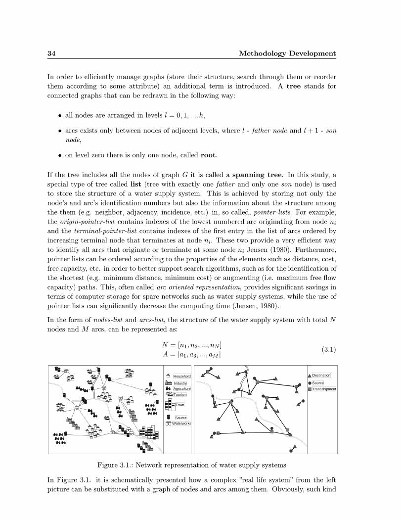
34 Methodology Development
In order to efficiently manage graphs (store their structure, search through them or reorder
them according to some attribute) an additional term is introduced. A tree stands for
connected graphs that can be redrawn in the following way:
• all nodes are arranged in levels l = 0, 1, ..., h,
• arcs exists only between nodes of adjacent levels, where l - father node and l + 1 - son
node,
• on level zero there is only one node, called root.
If the tree includes all the nodes of graph G it is called a spanning tree. In this study, a
special type of tree called list (tree with exactly one father and only one son node) is used
to store the structure of a water supply system. This is achieved by storing not only the
node’s and arc’s identification numbers but also the information about the structure among
the them (e.g. neighbor, adjacency, incidence, etc.) in, so called, pointer-lists. For example,
the origin-pointer-list contains indexes of the lowest numbered arc originating from node ni
and the terminal-pointer-list contains indexes of the first entry in the list of arcs ordered by
increasing terminal node that terminates at node ni. These two provide a very efficient way
to identify all arcs that originate or terminate at some node ni Jensen (1980). Furthermore,
pointer lists can be ordered according to the properties of the elements such as distance, cost,
free capacity, etc. in order to better support search algorithms, such as for the identification of
the shortest (e.g. minimum distance, minimum cost) or augmenting (i.e. maximum free flow
capacity) paths. This, often called arc oriented representation, provides significant savings in
terms of computer storage for spare networks such as water supply systems, while the use of
pointer lists can significantly decrease the computing time (Jensen, 1980).
In the form of nodes-list and arcs-list, the structure of the water supply system with total N
nodes and M arcs, can be represented as:
N = [n1, n2, ..., nN ]
A = [a1, a3, ..., aM ](3.1)
Tourism
Waterworks
Source
Agriculture
Household
Industry
Town
Transshipment
Source
Destination
Figure 3.1.: Network representation of water supply systems
In Figure 3.1. it is schematically presented how a complex ”real life system” from the left
picture can be substituted with a graph of nodes and arcs among them. Obviously, such kind
3.1 Representation of Water Supply Systems and Objectives of the Analysis 35
of simplifications have sense and value only for large water supply systems (mainly regional
ones) that have many different sources and delivery points, consist of many transport, storage
and treatment facilities and in which flow of water may take many different paths that can
not be easily identified and analysed by manual calculations.
3.1.2. Water Supply System’s Function
In addition to the possibility to represent the elements and the structure of a water supply
system, the Graph Theory enables for the representation of the element’s properties. Graph’s
arcs and nodes have attributes that may correspond to the properties of a real system, such
as capacities, lengths, costs, etc.. Due to the frequent use, graphs whose arcs have capacity
as an attribute have their own name, networks.
The exact definition of a network, as in Hartmann and Rieger (2002), that is based on the
assignment of some arbitrary functions on arcs or nodes, called labelling, fa : A → Q from
arcs to rational numbers and fn : N → S from nodes to arbitrary set reads as ”a network is
a tuple, or an ordered set of n elements, Gn = (G,κ, ns, nd, nt) where:
• G = (N,A) is a directed graph without arcs of the form aii,
• κ : A → R+0 is a positive labelling of arc capacities and κ(aij) = 0 if aij /∈ A,
• ns ∈ N is a node called source with no incoming di(ns) = 0 arcs,
• nd ∈ N is a node called destination with no outgoing do(nd) = 0 arcs,
• nt ∈ N is a node called transshipment with incoming di(nt) > 0 and outgoing do(nt) > 0
arcs”.
Flow of water over a network is an attribute of the arcs. It is usually denoted as xij and
represents the quantity of water flowing through an arc aij in a period of time. For a given
network Gn = (G,κ, ns, nd, nt) a set of flows on all arcs x = {xij | aij ∈ A} is referred as flow
vector or flow pattern. In addition, according to the previous definition of the path, a path
flow is a vector that corresponds to sending a positive amount of flow along arcs of a path,
or more precisely, it is a flow vector x with components of the form (Bertsekas, 1998):
xij =
⎧⎨
⎩
a if aij ∈ π+
−a if aij ∈ π−
0 otherwise
(3.2)
where a is a positive scalar and π+ and π− are the forward and backward paths. As proved
by Bertsekas (1998) ”any flow vector can be decomposed into a set of conforming paths”,
where a path flow xπ conforms to a flow vector x if it carries flow in the forward direction
(xij > 0 for all forward arcs and xij < 0 for all backward arcs on the path π ) and if a forward
path have a source and destination node as start and end node, respecitively. This simple
proposition can be extremely useful in the analysis of systems such as water supply systems,
where the main aim is exactly to analyse the water paths from source to destination nodes.
36 Methodology Development
Before further proceeding into the definition of the governing equations and their constraints,
the following simplifications can be made. Firstly, although different commodities (e.g. raw
water, treated water) may be transported over a water supply network, there is no need to
consider multi-commodity flows on water supply networks, since there are no arcs at which
two different commodities flow at the same time. And secondly, the conservation of flow in
arcs will be assumed and the pipe losses will be then additionally accounted for.
Under the assumptions that water in a water supply network is an incompressible fluid 2 and
that the temperature differences are small 3, the continuity and momentum equations are
sufficient to determine the velocities and pressures in a water supply network.
The momentum equation basically states that for any small, fixed control volume of fluid,
the rate of change of momentum must equal the sum of any external forces acting on the
control volume. In order to simplify the writing of momentum equation, for a constant
diameter pipe, the parameters that influence the forces of fluid weight, pressure and friction
are often represented by, so called, pipe characteristics rij :
rij = CτijLij
2gA3ij
∀aij (3.3)
where Lij - length of a pipe, Aij - cross section area of a pipe and Cτij - coefficient of tangential
friction (friction coefficient). Since the change of flow velocity in constant diameter pipe can
be approximated to zero for incompressible fluid, the change of momentum in control volume
is equal zero and the momentum equation is reduced to the summation of the forces and may
be written as in (Ivetic, 1996):
Πi −Πj = rijx2ij ∀aij or alternatively
Πi −Πj = rijxij |xij| ∀aij (3.4)
where Πi - is a head at node i and represents the sum of kinetic (pi-pressure) and potential
energy (zi-elevation over some reference point, usually sea level). Lower -λij and upper -κijcapacity bounds of the network arcs represent constraints that have to be respected.
xij ≤ κij ∀aij ∈ A
xij ≥ λij ∀aij ∈ A(3.5)
where lower bound λij is usually equal 0. For directed networks a negative flow constraint,
or so called skew symmetry constraint, must be fulfilled too.
xij = −xji ∀aij ∈ A (3.6)
2has constant density3small enough that no heat flux occur
3.1 Representation of Water Supply Systems and Objectives of the Analysis 37
In addition to water conservation in arcs, water has to be conserved on nodes too. Sum of
inflows must be equal to sum of outflows except on source and destination nodes where it
equals external flow. The continuity equation can be written as (Ivetic, 1996):
∑
nj
xij + bj = 0 ∀nj or alternatively
∑
nj :aij∈Axij −
∑
nj :aji∈Axji + bj = 0 ∀nj
(3.7)
where bj represent the external flow which comes in or leaves the system. For source nodes
bj > 0, for destination nodes bj < 0 and for transshipment nodes bj = 0. Consequently, these
values have to satisfy maximum available and minimum demanded water amounts at source
and demand nodes, respectively:
bj ≤ Smaxj ∀nsj ∈ N
bj ≥ Dminj ∀ndj ∈ N(3.8)
Finally, the total energy (Πi), or its kinetic component (pi-pressure) is mainly bounded by
engineering standards for satisfaction of users services and network safety which represents
the last constraint to the above defined equations:
pminj ≤ pj ≤ pmaxj ∀nj ∈ N (3.9)
It is important to mention that the term rij-pipe characteristics introduced in Equation 3.4
contains the friction coefficient expressed as tangential tension coefficient Cτ . There are many
other ways to express the friction losses in the momentum equation and the three most often
used will be mentioned here.
For example the Darcy-Weissbach friction coefficient λ, where λ = 4Cτ and for a circular
pipe (A/O = D/4) transforms the pipe characteristics to the:
rij = λij8Lij
gπ2D5ij
(3.10)
where Dij is a pipe diameter. Another very popular expression of the pipe characteristics is
a Hazen-Williams formula. Its friction coefficient C is not a function of velocity, is applicable
only to the water flows at ordinary temperatures (4− 20◦C) and has different flow exponent
in the momentum equation:
Πi −Πj = rijx1.852ij and rij = k4.727
Lij
C1.852ij D4.871
ij(3.11)
where k is a unit conversion factor: k = 1.318 for English and k = 0.85 for SI units. The third
most often used, is the Chezy-Manning friction coefficient n, for which the pipe characteristics
becomes:rij = k4.66n2 Lij
D5.33ij
(3.12)
The selection of one of these equation depends on the available network data and all of them
will be integrated in the latter developed models.
38 Methodology Development
3.1.3. Formulation of the Optimization Problem
After showing how to mathematically define the structure and the most important charac-
teristics of water supply systems, it is necessary to mathematically formulate the aims and
objectives of a water supply analysis. Since the most common understanding of the function
of water supply systems is to transport water through a network in order to satisfy demands
at the destination nodes form available supplies at the source nodes by providing a good
quality service to the users with the minimum costs and negative effects, in the most general
terms the aim of the water supply systems analyses can be stated as the cost minimisation
of network flows, often called Minimum Cost Network Flow problem. Bertsekas (1998)
defines this problem as: ”search for a set of arc flows that minimize a given cost function,
subject to the constraints that they produce a given divergence4 vector and that they lie
within some given bounds”. Due to the functional dependency of flows and network prop-
erties, the identification of flows that give a minimum cost over a network can be used to
identify the minimum cost layout, capacities, energy input, or some other network charac-
teristic. This flexibility makes the Minimum Cost Network Flow problem one of the most
often implemented optimization formulations in many engineering disciplines (Henley and
Williams, 1973; Biggs et al., 1976; Harary, 1994).
The Minimum Cost Network Flow problem, defined on arcs, for water supply networks can
be stated as:min z =
∑
aij∈Acijxij (3.13)
subject to: ∑
nj :aij∈Axij −
∑
nj :aji∈Axji = bj ∀nj ∈ N
xij ≤ κij ∀aij ∈ A
pminj ≤ pj ≤ pmaxj ∀nj ∈ N
(3.14)
Alternatively, if πk is defined as a conforming simple path5 out of total Π directed paths
between any pair of source-destination pairs, and xπk as a path flow6 on it, then the collection
of x = {xπk | πk ∈ Π} represents the network flow in path form. The whole network flow
can be represented as collection of conforming simple paths. The flows in individual arcs are
(Ahuja et al., 1993):
xij =∑
πk
δπkij x
πk (3.15)
where δπkij = 1 if aij is on path xπk and 0 otherwise.
4of a vector field is the rate at which ”density” exits a given region of space and in the absence of the creation
or destruction of matter, the density within a region of space can change only by having it flow into or out
of the region (Weisstein, 1999b)5directed path from source ns to destination nd node whose path flow is equal some quantity a, where xij = a
for forward arcs and xij = −a for backward arcs6amount of flow that is send from source node ns to destination node nd along path πk
3.2 Method for the Integration of Environmental and Socioeconomic Aspects 39
The formulation of the Minimum Cost Network Flow optimization problem in path form
states:min z =
∑
πk∈Π(xπk
∑
aij∈πk
cij) (3.16)
subject to: ∑
πk
δπkij x
πk ≤ κij ∀πk ∈ Π
pminj ≤ pj ≤ pmaxj ∀nj ∈ N(3.17)
Although arc form and path form are completely equivalent, the path form is adopted here
because it: a) determines flows in a more applicable way since in water supply systems water
is always sent from some source node to some destination node and b) reduces the number
of unknown variables since it uses path flows instead of arc flows as unknown variables. In
addition such path form formulation is particularly convenient for the iterative or algorithms
that build one solution on another since it allows ease reallocation of flows among alternative
paths7 keeping the delivery at the destination nodes constant.
Furthermore, the Minimum Cost Network Flow problem formulated in the path form does
not need for explicit consideration of continuity equation at intermediate nodes since the flow
is always conserved on conforming paths. The sum of flows has to match external flow value
only on source and demand nodes. The satisfaction of this constraint and the arc capacity
constraint together, is often referred as the feasibility of the solution:
∑
nj :aij∈Axij −
∑
nj :aji∈Axji = bj ∀nj = ns, nd
∑
πk
δπkij x
πk ≤ κij ∀πk ∈ Π(3.18)
In water supply system analysis, the satisfaction of the pressure constraint (equation 3.17)
in addition to the previous constraints is called the satisfiability of the solution:
∑
nj :aij∈Axij −
∑
nj :aji∈Axji = bj ∀nj = ns, nd
∑
πk
δπkij x
πk ≤ κij ∀πk ∈ Π
pminj ≤ pj ≤ pmaxj ∀nj ∈ N
(3.19)
3.2. Method for the Integration of Environmental and
Socioeconomic Aspects
From scenic beauty and recreational opportunities, through input into production processes
to the necessary drinking, health and sanitation medium, water provides a complex set of
values to individuals and benefits to the society, so called use values. At the same time, water
is inherent element of the environment and provide a variety of values for further development
of life on earth, so called non-use values. Beside beneficial, sometimes referred as positive,
water use values such as the contribution to better health and living standard or better living
7the ones that connect the same source-destination combination but have different set of arcs
40 Methodology Development
conditions for plants and animals, some damaging, or negative, water use values, such as
flooding, population migration, conflicts over water uses or decrease of biodiversity, can be
identified. As explained in subchapter 2.2 on page 12 in order to identify and quantify these
water use values as a consequence of some project or actions the functional dependencies
between some parameters of the systems and their environmental and socioeconomic impacts
will be used.
3.2.1. Representation of Water Supply System’s Impacts
In the previously stated general formulation of the Minimum Cost Network Flow problem
the term cost stands for the negative impacts that a water supply system may cause in
economic, environmental, social and quality of a services domain. Since the main aim of
man-made projects or actions is not the costs minimization but instead ”the maximization of
benefits keeping in mind cost considerations” (Walski et al., 2003), it is necessary to redefine
this term in order to include positive consequence (benefits). The simplest way to achieve
this is to use net-costs (c) defined as difference between negative and positive costs or
impacts:
c(x) = costs(x)− benefits(x) (3.20)
As discussed in the previous chapter, the identification and quantification of costs and benefits
of an engineering project from an economic, environmental, social and system’s quality point
of view is not an easy task and relay on approximation methods. Examples that have been
already applied in the analysis of water systems include statistical procedures (O’Neill, 1972;
Roy et al., 1992), use of Satisfaction or Performance Indexes (de Neufville, 1970; Hellstrom
et al., 2000; Seager, 2001; Foxon et al., 2002), use of Environmental Impact Assessment
(Munn, 2006; Gunnerson, 1977; Petts, 1999), Strategic Environmental Assessment (Therivel
and Partidario, 1996), Life Cycle Assessment (Curran, 1996; ISO, 1997; Tillman et al., 1999)
or Material Flow Analysis (Bringezu et al., 1997) method and modelling procedures for the
assessment of economic costs (Lindsey and Walski, 1982; Clark et al., 2002) or for assessment
of environmental impacts (Chadwick, 2002; Finnveden and Moberg, 2005). The collective
aim of all these methods is to identify some kind of functional relationship among system
properties and their direct or indirect impacts. Since the main focus of the presented study
are not the individual methods for the evaluation of the impacts of water supply systems,
but rather the development of the general framework that allows for an integrated analysis of
these impacts, it is assumed that the individual impacts (costs and benefits) can be expressed
as single-variable function of some system parameter. The typical forms of the parameter-
impact relationships, or net-cost functions are presented in Figure 3.2.
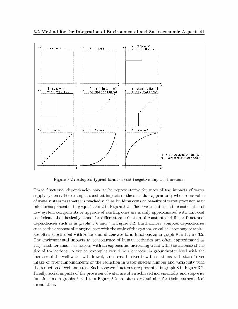
3.2 Method for the Integration of Environmental and Socioeconomic Aspects 41
Figure 3.2.: Adopted typical forms of cost (negative impact) functions
These functional dependencies have to be representative for most of the impacts of water
supply systems. For example, constant impacts or the ones that appear only when some value
of some system parameter is reached such as building costs or benefits of water provision may
take forms presented in graph 1 and 2 in Figure 3.2. The investment costs in construction of
new system components or upgrade of existing ones are mainly approximated with unit cost
coefficients that basically stand for different combination of constant and linear functional
dependencies such as in graphs 5, 6 and 7 in Figure 3.2. Furthermore, complex dependencies
such as the decrease of marginal cost with the scale of the system, so called“economy of scale“,
are often substituted with some kind of concave form functions as in graph 9 in Figure 3.2.
The environmental impacts as consequence of human activities are often approximated as
very small for small size actions with an exponential increasing trend with the increase of the
size of the actions. A typical examples would be a decrease in groundwater level with the
increase of the well water withdrawal, a decrease in river flow fluctuations with size of river
intake or river impoundments or the reduction in water species number and variability with
the reduction of wetland area. Such concave functions are presented in graph 8 in Figure 3.2.
Finally, social impacts of the provision of water are often achieved incrementally and step-wise
functions as in graphs 3 and 4 in Figure 3.2 are often very suitable for their mathematical
formulation.
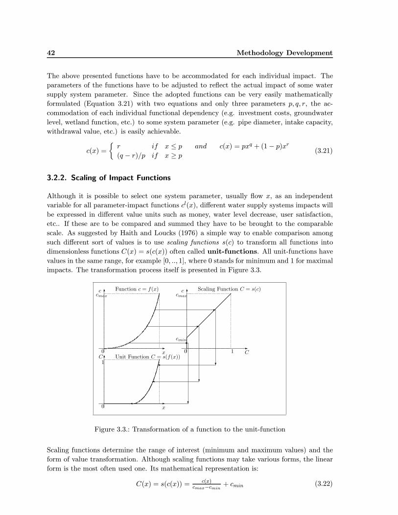
42 Methodology Development
The above presented functions have to be accommodated for each individual impact. The
parameters of the functions have to be adjusted to reflect the actual impact of some water
supply system parameter. Since the adopted functions can be very easily mathematically
formulated (Equation 3.21) with two equations and only three parameters p, q, r, the ac-
commodation of each individual functional dependency (e.g. investment costs, groundwater
level, wetland function, etc.) to some system parameter (e.g. pipe diameter, intake capacity,
withdrawal value, etc.) is easily achievable.
c(x) =
{r if x ≤ p and c(x) = pxq + (1− p)xr
(q − r)/p if x ≥ p(3.21)
3.2.2. Scaling of Impact Functions
Although it is possible to select one system parameter, usually flow x, as an independent
variable for all parameter-impact functions cl(x), different water supply systems impacts will
be expressed in different value units such as money, water level decrease, user satisfaction,
etc.. If these are to be compared and summed they have to be brought to the comparable
scale. As suggested by Haith and Loucks (1976) a simple way to enable comparison among
such different sort of values is to use scaling functions s(c) to transform all functions into
dimensionless functions C(x) = s(c(x)) often called unit-functions. All unit-functions have
values in the same range, for example [0, .., 1], where 0 stands for minimum and 1 for maximal
impacts. The transformation process itself is presented in Figure 3.3.
Function c = f(x)
�
�c
x0
cmax
Scaling Function C = s(c)
�
�
��
��
��
��
c
C0 1
cmax
cmin
Unit Function C = s(f(x))
�
�C
x0
1
�
�
�
�
�
�
�
�
�
Figure 3.3.: Transformation of a function to the unit-function
Scaling functions determine the range of interest (minimum and maximum values) and the
form of value transformation. Although scaling functions may take various forms, the linear
form is the most often used one. Its mathematical representation is:
C(x) = s(c(x)) = c(x)cmax−cmin
+ cmin (3.22)
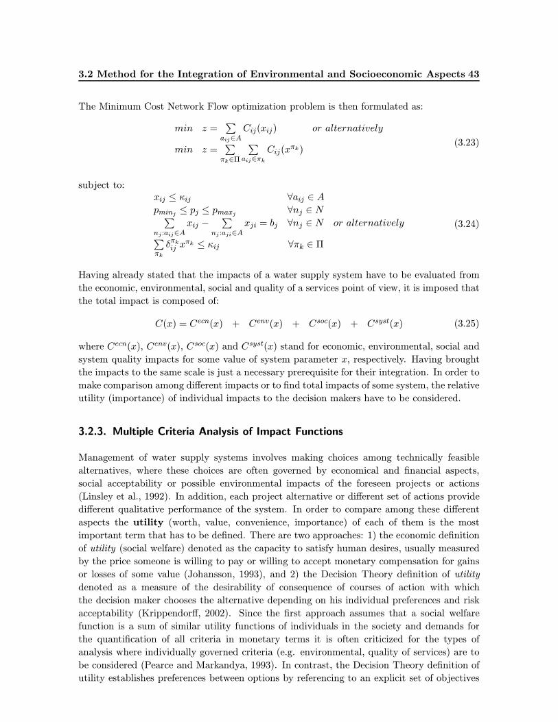
3.2 Method for the Integration of Environmental and Socioeconomic Aspects 43
The Minimum Cost Network Flow optimization problem is then formulated as:
min z =∑
aij∈ACij(xij) or alternatively
min z =∑
πk∈Π
∑
aij∈πk
Cij(xπk)
(3.23)
subject to:xij ≤ κij ∀aij ∈ A
pminj ≤ pj ≤ pmaxj ∀nj ∈ N∑
nj :aij∈Axij −
∑
nj :aji∈Axji = bj ∀nj ∈ N or alternatively
∑
πk
δπkij x
πk ≤ κij ∀πk ∈ Π
(3.24)
Having already stated that the impacts of a water supply system have to be evaluated from
the economic, environmental, social and quality of a services point of view, it is imposed that
the total impact is composed of:
C(x) = Cecn(x) + Cenv(x) + Csoc(x) + Csyst(x) (3.25)
where Cecn(x), Cenv(x), Csoc(x) and Csyst(x) stand for economic, environmental, social and
system quality impacts for some value of system parameter x, respectively. Having brought
the impacts to the same scale is just a necessary prerequisite for their integration. In order to
make comparison among different impacts or to find total impacts of some system, the relative
utility (importance) of individual impacts to the decision makers have to be considered.
3.2.3. Multiple Criteria Analysis of Impact Functions
Management of water supply systems involves making choices among technically feasible
alternatives, where these choices are often governed by economical and financial aspects,
social acceptability or possible environmental impacts of the foreseen projects or actions
(Linsley et al., 1992). In addition, each project alternative or different set of actions provide
different qualitative performance of the system. In order to compare among these different
aspects the utility (worth, value, convenience, importance) of each of them is the most
important term that has to be defined. There are two approaches: 1) the economic definition
of utility (social welfare) denoted as the capacity to satisfy human desires, usually measured
by the price someone is willing to pay or willing to accept monetary compensation for gains
or losses of some value (Johansson, 1993), and 2) the Decision Theory definition of utility
denoted as a measure of the desirability of consequence of courses of action with which
the decision maker chooses the alternative depending on his individual preferences and risk
acceptability (Krippendorff, 2002). Since the first approach assumes that a social welfare
function is a sum of similar utility functions of individuals in the society and demands for
the quantification of all criteria in monetary terms it is often criticized for the types of
analysis where individually governed criteria (e.g. environmental, quality of services) are to
be considered (Pearce and Markandya, 1993). In contrast, the Decision Theory definition of
utility establishes preferences between options by referencing to an explicit set of objectives
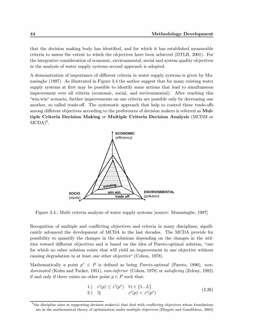
44 Methodology Development
that the decision making body has identified, and for which it has established measurable
criteria to assess the extent to which the objectives have been achieved (DTLR, 2001). For
the integrative consideration of economic, environmental, social and system quality objectives
in the analysis of water supply systems second approach is adopted.
A demonstration of importance of different criteria in water supply systems is given by Mu-
nasinghe (1997). As illustrated in Figure 3.4 the author suggest that for many existing water
supply systems at first may be possible to identify some actions that lead to simultaneous
improvement over all criteria (economic, social, and environmental). After reaching this
“win-win“ scenario, further improvements on one criteria are possible only by decreasing one
another, so called trade-off. The systematic approach that help to control these trade-offs
among different objectives according to the preferences of decision makers is referred as Mul-
tiple Criteria Decision Making or Multiple Criteria Decision Analysis (MCDM or
MCDA)8.
ECONOMIC(efficiency)
ENVIRONMENTAL(pollution)
SOCIO(equity)
existing
win wintrade off
Figure 3.4.: Multi criteria analysis of water supply systems [source: Munasinghe, 1997]
Recognition of multiple and conflicting objectives and criteria in many disciplines, signifi-
cantly advanced the development of MCDA in the last decades. The MCDA provide for
possibility to quantify the changes in the solutions depending on the changes in the util-
ities toward different objectives and is based on the idea of Pareto-optimal solution, “one
for which no other solution exists that will yield an improvement in one objective without
causing degradation in at least one other objective“ (Cohon, 1978).
Mathematically a point p∗ ∈ P is defined as being Pareto-optimal (Pareto, 1896), non-
dominated (Kuhn and Tucker, 1951), non-inferior (Cohon, 1978) or satisficing (Zeleny, 1982)
if and only if there exists no other point p ∈ P such that:
1.) zi(p) ≤ zi(p∗) ∀i ∈ {1...L}2.) ∃j zj(p) < zj(p∗)
(3.26)
8the discipline aims at supporting decision maker(s) that deal with conflicting objectives whose foundations
are in the mathematical theory of optimization under multiple objectives (Ehrgott and Gandibleux, 2003)
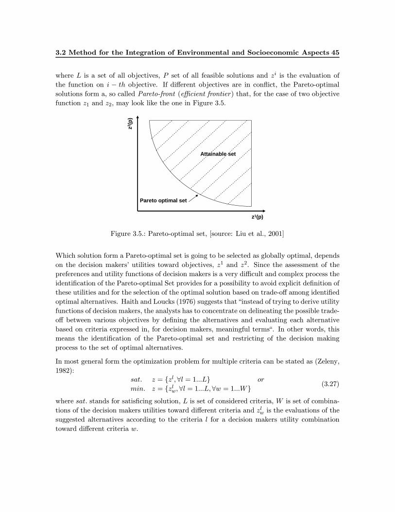
3.2 Method for the Integration of Environmental and Socioeconomic Aspects 45
where L is a set of all objectives, P set of all feasible solutions and zi is the evaluation of
the function on i − th objective. If different objectives are in conflict, the Pareto-optimal
solutions form a, so called Pareto-front (efficient frontier) that, for the case of two objective
function z1 and z2, may look like the one in Figure 3.5.
Pareto optimal set
Attainable set
z1(p)
z2(p
)
Figure 3.5.: Pareto-optimal set, [source: Liu et al., 2001]
Which solution form a Pareto-optimal set is going to be selected as globally optimal, depends
on the decision makers’ utilities toward objectives, z1 and z2. Since the assessment of the
preferences and utility functions of decision makers is a very difficult and complex process the
identification of the Pareto-optimal Set provides for a possibility to avoid explicit definition of
these utilities and for the selection of the optimal solution based on trade-off among identified
optimal alternatives. Haith and Loucks (1976) suggests that“instead of trying to derive utility
functions of decision makers, the analysts has to concentrate on delineating the possible trade-
off between various objectives by defining the alternatives and evaluating each alternative
based on criteria expressed in, for decision makers, meaningful terms“. In other words, this
means the identification of the Pareto-optimal set and restricting of the decision making
process to the set of optimal alternatives.
In most general form the optimization problem for multiple criteria can be stated as (Zeleny,
1982):
sat. z = {zl,∀l = 1...L} or
min. z = {zlw,∀l = 1...L,∀w = 1...W} (3.27)
where sat. stands for satisficing solution, L is set of considered criteria, W is set of combina-
tions of the decision makers utilities toward different criteria and zlw is the evaluations of the
suggested alternatives according to the criteria l for a decision makers utility combination
toward different criteria w.
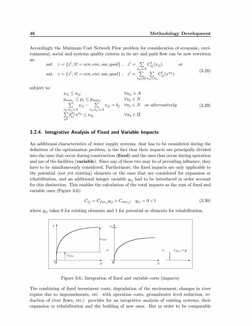
46 Methodology Development
Accordingly the Minimum Cost Network Flow problem for consideration of economic, envi-
ronmental, social and systems quality criteria in its arc and path flow can be now rewritten
as:sat. z = {zl,∀l = ecn, env, soc, qual} , zl =
∑
aij∈AC lij(xij) or
sat. z = {zl,∀l = ecn, env, soc, qual} , zl =∑
πk∈Π
∑
aij∈πk
C lij(x
πk)(3.28)
subject to:xij ≤ κij ∀aij ∈ A
pminj ≤ pj ≤ pmaxj ∀nj ∈ N∑
nj :aij∈Axij −
∑
nj :aji∈Axji = bj ∀nj ∈ N or alternatively
∑
πk
δπkij x
πk ≤ κij ∀πk ∈ Π
(3.29)
3.2.4. Integrative Analysis of Fixed and Variable Impacts
An additional characteristics of water supply systems, that has to be considered during the
definition of the optimization problem, is the fact that their impacts are principally divided
into the ones that occur during construction (fixed) and the ones that occur during operation
and use of the facilities (variable). Since any of these two may be of prevailing influence, they
have to be simultaneously considered. Furthermore, the fixed impacts are only applicable to
the potential (not yet existing) elements or the ones that are considered for expansion or
rehabilitation, and an additional integer variable yij had to be introduced in order account
for this distinction. This enables the calculation of the total impacts as the sum of fixed and
variable ones (Figure 3.6):
Cij = Cfixijyij + Cvarij ; yij = 0 ∨ 1 (3.30)
where yij takes 0 for existing elements and 1 for potential or elements for rehabilitation.
�
�c
x0
cfix
cvar
�
�
�
�cvar
x0
= + cfix ∗ y
�
Figure 3.6.: Integration of fixed and variable costs (impacts)
The combining of fixed investment costs, degradation of the environment, changes in river
regime due to impoundments, etc. with operation costs, groundwater level reduction, re-
duction of river flows, etc.) provides for an integrative analysis of existing systems, their
expansion or rehabilitation and the building of new ones. But in order to be comparable
3.2 Method for the Integration of Environmental and Socioeconomic Aspects 47
fixed and variable impacts have to be brought to the same time horizon. For example eco-
nomic consequence of water supply are assessed in months or years while some environmental
impacts may last for thousands of years.
The economic values are brought to the same time scale mainly by using the Time Value of
Money concept. It is based on the premise that most people prefer to receive money today,
rather than the same amount in the future. The difference in the value of money today (PV )
and in some future time (FV ) is caused by opportunity cots (i.e. loss of value since money
is not put to productive use) and risk over time (e.g. risk of inflation). In Time Value of
Money calculations these two are expressed with the interest rate (r). For some time period
n with the constants interest rate r the present (PV ) and the future value of money (FV )
can be equated using following formulas (Copeland et al., 1998):
PV = FV(1+r)n and FV = PV (1 + r)n (3.31)
Since the future benefits and costs are usually not a single value but rather a stream of values
(e.g. credit payments, operation costs, etc.) the time value of money are usually expressed
to their annuity (A) (Copeland et al., 1998):
PV A = A1− 1
(1+r)n
r and FV A = A (1+r)n−1r
(3.32)
where PV A-present value to an annuity, FV A-future value to an annuity and A-is the annuity
or the individual value in each compounding9 period.
Based on this it is possible to discount the value of a projects, company or anything else
for which some nominal future value (FV ) can be defined to the appropriate present value
(DPV ) simply by summing its successive present values in compounding periods t (Copeland
et al., 1998):
DPV =t=0∑
t=n
FVt(1+r)t
(3.33)
Adapting a multi-objective approach, Loucks and Gladwell (1999) suggested to use the
weighted sum of successive future present values in order to encompass the different value of
money in different time periods.
DPV =t=0∑
t=nat
FVt(1+r)t
(3.34)
where at is a weight of present values of in period t and∑
at = 1; t ∈ 1, ..n.
Such a formulation of discounted present value of some future costs is very flexible in terms
of setting the preferences toward future benefits and costs and can be easily adopted for the
discounting of environmental and social impacts too. Only, the interest rate (r), or discount
rate, has to be accommodated to encompass the opportunity and risk of environmental and
social aspects. Unfortunately this can not be done with the certainty. But looking at the
current trends and preferences of our society it may be assumed that the environmental
9length of time in which an asset can generate cost or benefits
48 Methodology Development
and social aspects will obtain ever greater importance. To some degree this can be then
represented with greater interest rates.
For the introduced notation the discounting of the variable impacts can be written as:
DCvar =t=0∑
t=nat
Cvar(1+r)t
(3.35)
where DCvar-are discounted variable impacts to the present value, r-interest(discount) rate,
n total number of time periods t, Cvar-variable impacts in future time periods and at their
corresponding weights.
Together with the introduced yij variable, the Minimum Cost Network Flow problem in its
arc and path form can be now stated as:
sat. z = {zl,∀l = ecn, env, soc, qual}, zl =∑
aij∈A(DC l
varij (xij) + C lfixij
(xij)yij) or
sat. z = {zl,∀l = ecn, env, soc, qual} , zl =∑
πk∈Π
∑
aij∈πk
(DC lvarij (x
πk) + C lfixij
(xπk)yij)
(3.36)
subject to:xij ≤ κijyij ∀aij ∈ A
pminj ≤ pj ≤ pmaxj ∀nj ∈ N∑
nj :aij∈Axij −
∑
nj :aji∈Axji = bj ∀nj ∈ N or alternatively
∑
πk
δπkij x
πk ≤ κijyij ∀πk ∈ Π
yij = 0 ∨ 1 ∀aij ∈ A
(3.37)
At the end it is important to stress that the inclusion of the discrete variable yij renders
defined optimisation problem as a multi-variable one. This means that beside the flows (xij),
the configuration of a network (yij) is also variable and have to be optimised. Since the
configuration of a network controls its flows, it is suggested to decompose the problem and
use one algorithm to create, evaluate and identify optimal network configuration and another
one to identify the minimum cost flow solution for each of these configurations.
3.3 Methods for the Solution of the Optimisation Problem 49
3.3. Methods for the Solution of the Optimisation Problem
Numerous optimization techniques that have been successfully applied for the Minimum Cost
Network Flow problem can be divided in three general categories (Bertsekas, 1998):
1. Primal cost improvement - iterative improvement of costs by constructing sequence of
feasible flows,
2. Dual cost improvement - iterative improvement of dual costs by constructing sequence
of prices10.
3. Auction - generation of prices in a way that is reminiscent to real-life auctions but in
addition to prices the algorithms iterate on flows, too11.
In general they are all iterative procedures to obtain a solution of an optimization problem
that satisfies the constraint conditions and the principal difference is the order in which the
”closeness” to the optimum and the constraint conditions are satisfied (Jensen, 1980). Due
to the fact that each of them is more convenient for a slightly different type of problem the
prime criteria in the selection of optimization technique are the characteristics of the problem
itself.
3.3.1. Characteristics of the Optimisation Problem
A prime characteristic that distinguishes the defined Minimum Cost Network Flow Problem
from a standard one, ”a least cost shipment of a commodity through a network in order to
satisfy demands at certain nodes form available supplies at other nodes” (Bertsekas, 1998), is
the implementation of linear, step-wise, convex and concave functions instead of cost coeffi-
cients. Most network algorithms are appropriate, or efficient, only for the linear cost functions
because they select the direction of the search based on the gradients of the function at the
point under the examination. The left graph in Figure 3.7 shows how convex functions can
be approximated with many subsequent linear functions since the gradients of these new
functions can be ordered in an increasing, or at least monotony non-decreasing, order.
10the original network problem, called primal, can be transformed to another problem, called dual, by trans-
forming the constraints to the decision variables, called prices, and the decision variables to the constraints.
The dual costs represent the difference between original costs and newly formed prices and if the original
problem minimise costs than the dual problem maximise its dual costs (Bertsekas, 1998)11the dependency between flows and prices and the termination of the algorithm is based on a property called
complementary slackness that state that a solution is optimal if its primal and dual variables equal their
primal and dual constraints at the same time (Minieka, 1978)
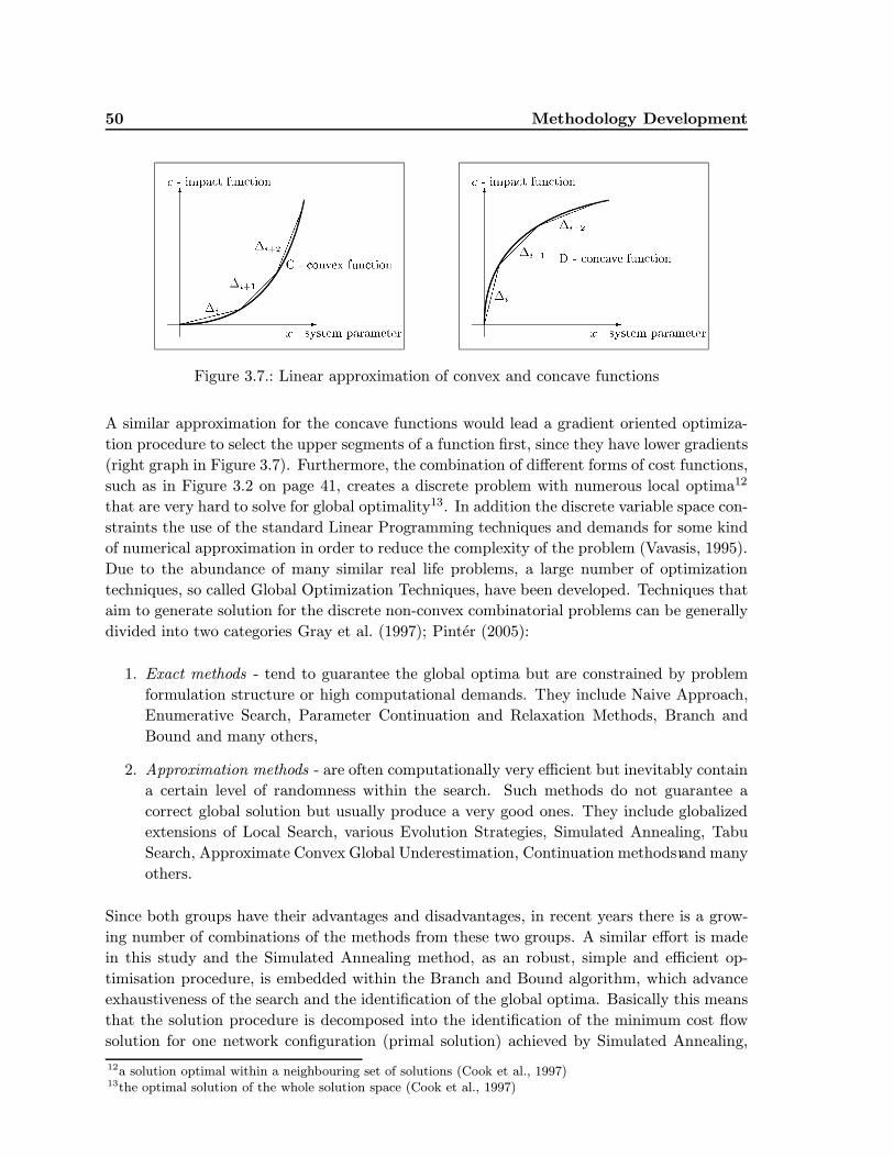
50 Methodology Development
Figure 3.7.: Linear approximation of convex and concave functions
A similar approximation for the concave functions would lead a gradient oriented optimiza-
tion procedure to select the upper segments of a function first, since they have lower gradients
(right graph in Figure 3.7). Furthermore, the combination of different forms of cost functions,
such as in Figure 3.2 on page 41, creates a discrete problem with numerous local optima12
that are very hard to solve for global optimality13. In addition the discrete variable space con-
straints the use of the standard Linear Programming techniques and demands for some kind
of numerical approximation in order to reduce the complexity of the problem (Vavasis, 1995).
Due to the abundance of many similar real life problems, a large number of optimization
techniques, so called Global Optimization Techniques, have been developed. Techniques that
aim to generate solution for the discrete non-convex combinatorial problems can be generally
divided into two categories Gray et al. (1997); Pinter (2005):
1. Exact methods - tend to guarantee the global optima but are constrained by problem
formulation structure or high computational demands. They include Naive Approach,
Enumerative Search, Parameter Continuation and Relaxation Methods, Branch and
Bound and many others,
2. Approximation methods - are often computationally very efficient but inevitably contain
a certain level of randomness within the search. Such methods do not guarantee a
correct global solution but usually produce a very good ones. They include globalized
extensions of Local Search, various Evolution Strategies, Simulated Annealing, Tabu
Search, Approximate Convex Global Underestimation, Continuation methods and many
others.
Since both groups have their advantages and disadvantages, in recent years there is a grow-
ing number of combinations of the methods from these two groups. A similar effort is made
in this study and the Simulated Annealing method, as an robust, simple and efficient op-
timisation procedure, is embedded within the Branch and Bound algorithm, which advance
exhaustiveness of the search and the identification of the global optima. Basically this means
that the solution procedure is decomposed into the identification of the minimum cost flow
solution for one network configuration (primal solution) achieved by Simulated Annealing,
12a solution optimal within a neighbouring set of solutions (Cook et al., 1997)13the optimal solution of the whole solution space (Cook et al., 1997)
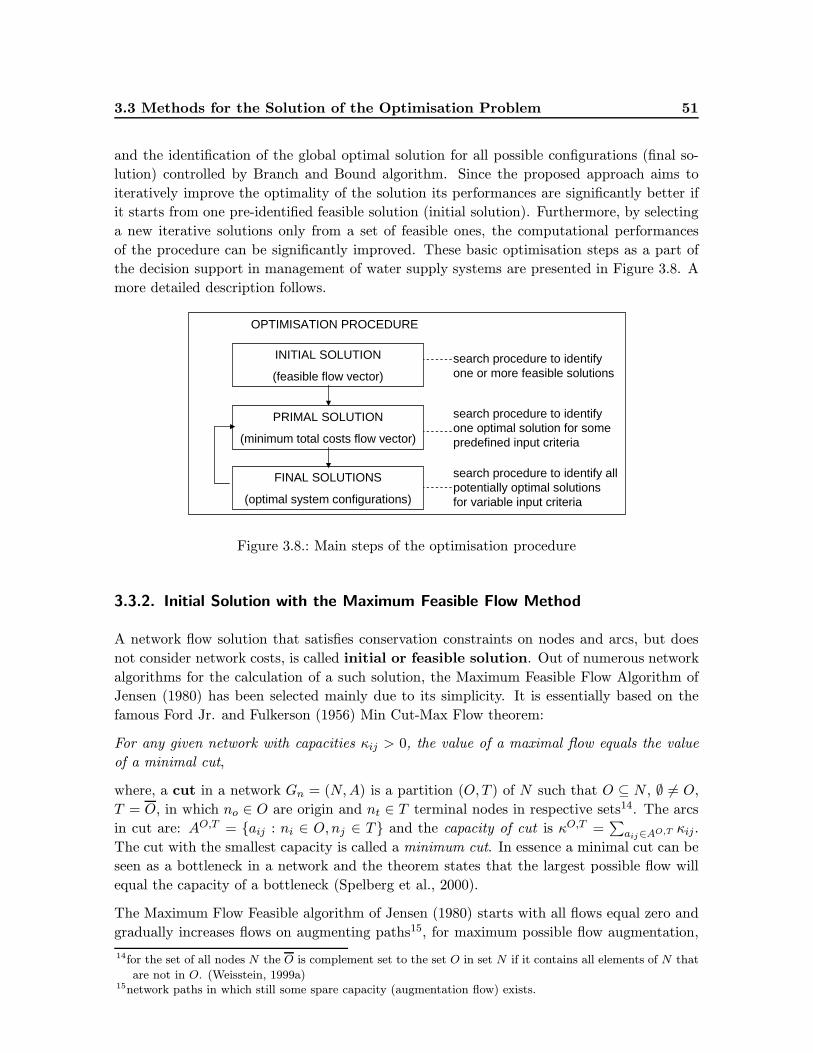
3.3 Methods for the Solution of the Optimisation Problem 51
and the identification of the global optimal solution for all possible configurations (final so-
lution) controlled by Branch and Bound algorithm. Since the proposed approach aims to
iteratively improve the optimality of the solution its performances are significantly better if
it starts from one pre-identified feasible solution (initial solution). Furthermore, by selecting
a new iterative solutions only from a set of feasible ones, the computational performances
of the procedure can be significantly improved. These basic optimisation steps as a part of
the decision support in management of water supply systems are presented in Figure 3.8. A
more detailed description follows.
INITIAL SOLUTION
(feasible flow vector)
PRIMAL SOLUTION
(minimum total costs flow vector)
FINAL SOLUTIONS
(optimal system configurations)
OPTIMISATION PROCEDURE
search procedure to identify one or more feasible solutions
search procedure to identify one optimal solution for some predefined input criteria
search procedure to identify all potentially optimal solutions for variable input criteria
Figure 3.8.: Main steps of the optimisation procedure
3.3.2. Initial Solution with the Maximum Feasible Flow Method
A network flow solution that satisfies conservation constraints on nodes and arcs, but does
not consider network costs, is called initial or feasible solution. Out of numerous network
algorithms for the calculation of a such solution, the Maximum Feasible Flow Algorithm of
Jensen (1980) has been selected mainly due to its simplicity. It is essentially based on the
famous Ford Jr. and Fulkerson (1956) Min Cut-Max Flow theorem:
For any given network with capacities κij > 0, the value of a maximal flow equals the value
of a minimal cut,
where, a cut in a network Gn = (N,A) is a partition (O,T ) of N such that O ⊆ N , ∅ = O,
T = O, in which no ∈ O are origin and nt ∈ T terminal nodes in respective sets14. The arcs
in cut are: AO,T = {aij : ni ∈ O,nj ∈ T} and the capacity of cut is κO,T =∑
aij∈AO,T κij.
The cut with the smallest capacity is called a minimum cut. In essence a minimal cut can be
seen as a bottleneck in a network and the theorem states that the largest possible flow will
equal the capacity of a bottleneck (Spelberg et al., 2000).
The Maximum Flow Feasible algorithm of Jensen (1980) starts with all flows equal zero and
gradually increases flows on augmenting paths15, for maximum possible flow augmentation,
14for the set of all nodes N the O is complement set to the set O in set N if it contains all elements of N that
are not in O. (Weisstein, 1999a)15network paths in which still some spare capacity (augmentation flow) exists.
52 Methodology Development
till the bottleneck capacity is reached. Augmenting actually increases the network flows on
forward and decreases them on backward arcs since the later ones have a negative flow value.
The procedure is executed for all pair of nodes, one with unsatisfied positive and another with
unsatisfied negative external flow until all external flows are satisfied or all path capacities
are used to their maximum flow. At the end, if all external flows are not satisfied then a
feasible solution of a problem does not exist. In order to deal with this an additional node, so
called slack node, is introduced. This virtual node is with virtual arcs, slack arcs, connected
with all source and demand nodes in order to accept the surplus and provide for the deficient
external flows. The flow is routed to slack node only when all other node pairs are exhausted
and total flow in it serves as the indication of the feasibility of a solution. Basic steps of the
Maximum Feasible Flow Method are the following (Jensen, 1980):
1. Initialize - Set all arc flows to null xij = 0, ∀xij ∈ A, create slack node nS and slack
arcs form every source node to slack node asS, ∀ns ∈ N and from slack node to every
destination node aSd, ∀nd ∈ N .
2. Maximum flow - Find a node pair (ns, nd) with positive external flow on source and
negative external flow on destination node and with still unsatisfied external flows,
establish an augmenting path πa among them and augment maximum flow amount
possible xπa = Min(| bs |, | bd |,Max(κij ,∀aij ∈ πa)). Reduce the magnitude of
the unsatisfied external flows at source and destination nodes for the augmented flow
amount | bs |=| bs | −xπa , | bd |=| bd | −xπa.
3. Control - If external flow is not satisfied on either source bs > 0 or demand node bd < 0,
search for another complementary node (demand for source node and source for demand
node) and repeat the step two for this new node pair. Since the algorithm does not leave
a node before it satisfies its external flow, after ”visiting” every source and destination
node for at least once the algorithm should find a feasible solution. If all nodes have
been already examined and the external flow at some node is still not satisfied, the
algorithm establish a path to the slack node and allocate unsatisfied flow to this path.
As previously stated the total water flow at the slack node bS is an indicator of the feasibility
of the solution. It is equal the sum of flows on all slack arcs and is calculated by the following
formula:
bS =∑
nj :aSj∈AxSj −
∑
nj :ajS∈AxjS ∀nj = ns, nd (3.38)
bS = 0 shows than the total supply and demand external flows are equal and the feasible
solution on the network has been found. bS > 0 shows the existence of surplus supply for the
found feasible solution and bS < 0 the existence of demands which can not be satisfied due to
not enough supplies or capacities on a network. Since the usual approach for identification of
the network optimal solution is to start with the network configuration with the maximum
potential element’s number and sizes and then try to gradually reduce the costs by reducing
element’s sizes or taking some elements out of the network, if there is no feasible solution
for the first configuration there will be no feasible solutions for all others too. This has to
be corrected, either by adding new potential elements or by increasing the set of element’s
potential sizes, before further proceeding in the optimization procedure.
3.3 Methods for the Solution of the Optimisation Problem 53
3.3.3. Primal Solution with the Simulated Annealing Method
The procedure for the identification of a minimum cost flow solution for one system configu-
ration, referred as the primal solution, has to deal with a discrete network problem defined
on linear, step-wise, convex and concave cost functions. Even more, the procedure has to
be robust enough to handle many instances of local optima, many different constraints (e.g.
capacity of arcs, continuity on nodes, pressures in network, etc.), different initial conditions
(existing and new systems) and to allow accommodation for different types of optimization
problems (i.e. planning, design, operation problem).
Among various heuristic procedures the Simulated Annealing (Kirkpatrick et al., 1983; Cerny,
1985) is selected mainly due to its conceptual simplicity and proved robustness. Similarly as
heat induce atoms of crystals to wander randomly through the states of higher energy until
they find a state with the lower one, Simulated Annealing uses Metropolis-Hastings algorithm
(Metropolis et al., 1953; Hastings, 1970) to ultimately move to the better point (one with
lower energy state) and probabilistically evaluate the possibility to accept the worse point (one
with higher energy state) too. The used probability is described with the Maxwell-Boltzmann
distribution that imitates the exponential reduction of the energy variations (corresponds to
the acceptance of the worse point) with the reduction of the temperature of gases. This
allows Simulated Annealing to go uphill and downhill at the beginning in very large steps
and then by reducing the probability of accepting the uphill move to focus on finding an
optimal solution. Beside the temperature change, or so called cooling-schedule that must
allow the algorithm to make enough uphill and downhill moves in order to identify global
optima, second critical parameter is the neighbourhood function or the way of creating of new
random points. This function is application specific and, in order to achieve the effective
use of the method, it has to be accommodated in a way that the difference between old
and new points is in the same order of magnitude as the probability of acceptance of the
worse points. This is where it is possible to use the advantage of the graph representation of
water supply systems and instead of random creation of new points (flows on individual arcs),
use the simple conforming paths to effectively create new feasible solutions by exchanging
flow on alternative paths. In addition, for each randomly created flow change the selection
of the alternative augmenting paths can be improved by identifying the current minimum
cost ones and their prioritising. Keeping in mind that the identification of the optimal
solution is computationally very demanding (demands simultaneous examination of all source-
demand node combinations), the introduced improvement in the direction of the search and
the constraint to the feasible range only, significantly advance the total efficiency of the
algorithm. Moreover, the independence from the initial solution and the convergence of the
algorithm, are additionally improved by extending the Simulated Annealing to simultaneously
iterate on a set of solutions X = (x1,x2, ...,xN) instead on working on only one solution.
The main steps of the used Simulated Annealing method are the following:
1. Initialize - Starting from one feasible solution, create a set of N initial solutions X′
by randomly exchanging the flow on conforming simple paths xπ for all source-demand
nodes combinations Π. These set of randomly created solutions and the set of their
function values Z ′, represent the starting points for the rest of the algorithm. Set
54 Methodology Development
the Simulated Annealing schedule parameters: Tmax - initial temperature, ΔT - tem-
perature decrease parameter, Tmin - lowest temperature, Nmax - maximal number of
changes at each temperature and Nsuc - maximal number of successful changes at each
temperature T 16.
2. Change - For every solution x′ from a set X ′ invoke a random flow change Δxi on
all network paths xπi , ∀xπi ∈ Π, identify the set of all augmenting paths that can
compensate this change ΠA and find the one xπj with the minimum cost path flow
change Δzπj = Min(zπk (xπk + Δx) − zπk (x
πk)),∀xπk ∈ ΠA. By reallocation the flows
Δxi from the paths xπi to their minimum cost augmenting paths xπj for all source-
destination combinations ∀xπi ∈ Π, a new solution x′′ is created. Its function value
z′′ and the difference from the previous solution Δz = z′′ − z′ are calculated and the
acceptance is evaluated according to the following probability (Metropolis et al., 1953):
P =
{1 if Δz ≤ 0
e−Δz/BT if Δz > 0(3.39)
where T is the temperature at the current energy level ˙ and B is constant that relates
temperature to the function value (similar to Boltzmann’s constant for temperature
and energy). If Δz < 0 the probability P is greater then 1 and the method accept
this change, while for Δz > 0 probability depends on the current temperature of the
algorithm. Since the temperature reduces with each new energy level of the algorithm
(cooling schedule), the above stated probability also reduces with the progressing of the
algorithm. At each temperature the creation of the new solutions x′′ and evaluation of
their acceptance is repeated until the maximal number of changes (Nmax) or maximal
number of successful changes (Nsuc) is reached.
3. Evaluate - The newly created set of solutions X′′ = (x′′1,x
′′2, ...,x
′′N) with its function
values set Z ′′ = (z′′1 , z′′2 , ..., z
′′N ) is sorted in an increasing order list Z ′′ = [z′′1 , z
′′2 , ..., z
′′N ]
and if minimum temperature is reached T ≤ Tmin the solution at the first place is
the optimal one. If the temperature is greater than the minimum one T ≥ Tmin it is
decreased according to the cooling schedule (geometric temperature decrease T = T∗ΔT
is adopted) and steps 2. and 3. are repeated.
As proved by theoretical studies of Gidas (1985), the Simulated Annealing procedure con-
verges to an optimal solution if and only if the control parameter (temperature T ) is decreased
according to the following function:
T = Q/log(T ) (3.40)
where T and T are the temperature values at the consecutive energy levels and Q is a constant
term depending on the depth of local minimum generated by the transformation used to pass
form one solution to another. Since, the depth of a local minima is hard to assess in advance
and the temperature decrease according to the above formula requires exponential number
16the temperature corresponds to the energy level and will be noted with the indices ˙ while the iterations at
one temperature will be noted with the ′ indices
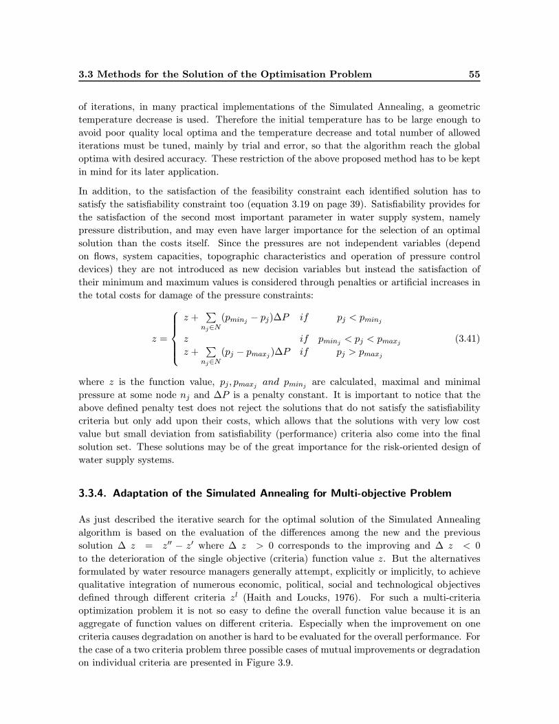
3.3 Methods for the Solution of the Optimisation Problem 55
of iterations, in many practical implementations of the Simulated Annealing, a geometric
temperature decrease is used. Therefore the initial temperature has to be large enough to
avoid poor quality local optima and the temperature decrease and total number of allowed
iterations must be tuned, mainly by trial and error, so that the algorithm reach the global
optima with desired accuracy. These restriction of the above proposed method has to be kept
in mind for its later application.
In addition, to the satisfaction of the feasibility constraint each identified solution has to
satisfy the satisfiability constraint too (equation 3.19 on page 39). Satisfiability provides for
the satisfaction of the second most important parameter in water supply system, namely
pressure distribution, and may even have larger importance for the selection of an optimal
solution than the costs itself. Since the pressures are not independent variables (depend
on flows, system capacities, topographic characteristics and operation of pressure control
devices) they are not introduced as new decision variables but instead the satisfaction of
their minimum and maximum values is considered through penalties or artificial increases in
the total costs for damage of the pressure constraints:
z =
⎧⎪⎪⎪⎨
⎪⎪⎪⎩
z +∑
nj∈N(pminj − pj)ΔP if pj < pminj
z if pminj < pj < pmaxj
z +∑
nj∈N(pj − pmaxj )ΔP if pj > pmaxj
(3.41)
where z is the function value, pj, pmaxj and pminj are calculated, maximal and minimal
pressure at some node nj and ΔP is a penalty constant. It is important to notice that the
above defined penalty test does not reject the solutions that do not satisfy the satisfiability
criteria but only add upon their costs, which allows that the solutions with very low cost
value but small deviation from satisfiability (performance) criteria also come into the final
solution set. These solutions may be of the great importance for the risk-oriented design of
water supply systems.
3.3.4. Adaptation of the Simulated Annealing for Multi-objective Problem
As just described the iterative search for the optimal solution of the Simulated Annealing
algorithm is based on the evaluation of the differences among the new and the previous
solution Δ z = z′′ − z′ where Δ z > 0 corresponds to the improving and Δ z < 0
to the deterioration of the single objective (criteria) function value z. But the alternatives
formulated by water resource managers generally attempt, explicitly or implicitly, to achieve
qualitative integration of numerous economic, political, social and technological objectives
defined through different criteria zl (Haith and Loucks, 1976). For such a multi-criteria
optimization problem it is not so easy to define the overall function value because it is an
aggregate of function values on different criteria. Especially when the improvement on one
criteria causes degradation on another is hard to be evaluated for the overall performance. For
the case of a two criteria problem three possible cases of mutual improvements or degradation
on individual criteria are presented in Figure 3.9.
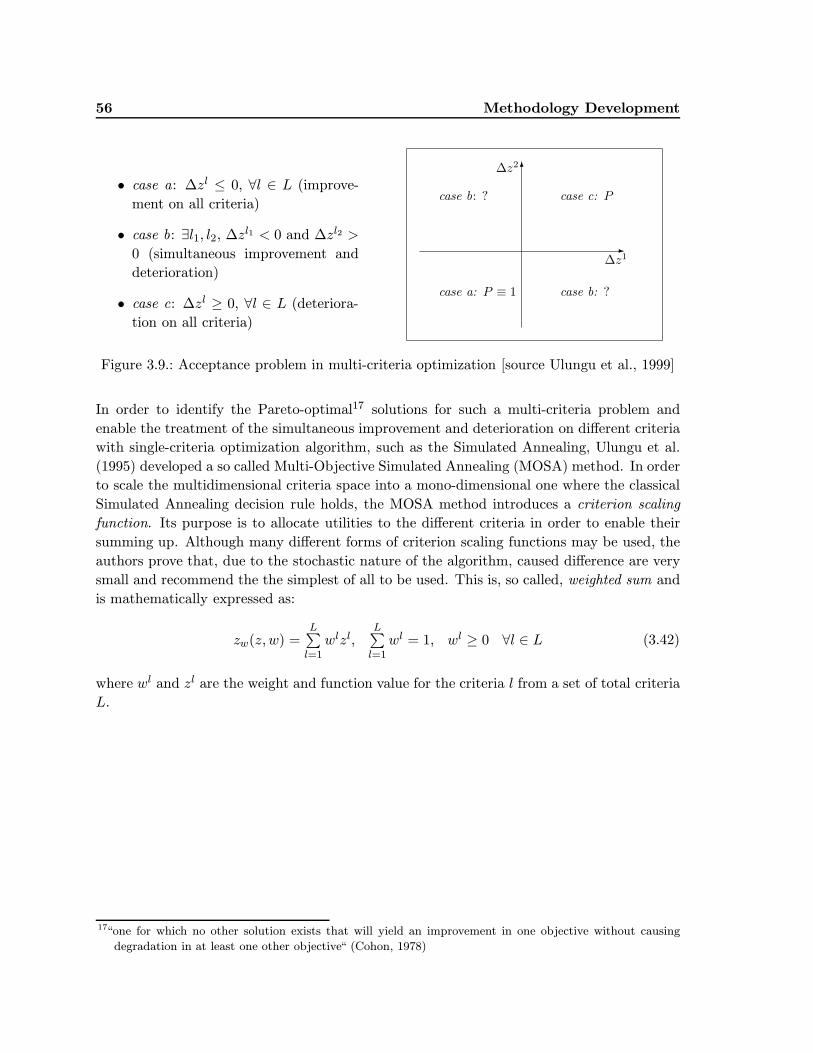
56 Methodology Development
• case a: Δzl ≤ 0, ∀l ∈ L (improve-
ment on all criteria)
• case b: ∃l1, l2, Δzl1 < 0 and Δzl2 >
0 (simultaneous improvement and
deterioration)
• case c: Δzl ≥ 0, ∀l ∈ L (deteriora-
tion on all criteria)
�
�
case c: Pcase b: ?
case a: P ≡ 1 case b: ?
Δz2
Δz1
Figure 3.9.: Acceptance problem in multi-criteria optimization [source Ulungu et al., 1999]
In order to identify the Pareto-optimal17 solutions for such a multi-criteria problem and
enable the treatment of the simultaneous improvement and deterioration on different criteria
with single-criteria optimization algorithm, such as the Simulated Annealing, Ulungu et al.
(1995) developed a so called Multi-Objective Simulated Annealing (MOSA) method. In order
to scale the multidimensional criteria space into a mono-dimensional one where the classical
Simulated Annealing decision rule holds, the MOSA method introduces a criterion scaling
function. Its purpose is to allocate utilities to the different criteria in order to enable their
summing up. Although many different forms of criterion scaling functions may be used, the
authors prove that, due to the stochastic nature of the algorithm, caused difference are very
small and recommend the the simplest of all to be used. This is, so called, weighted sum and
is mathematically expressed as:
zw(z, w) =L∑
l=1
wlzl,L∑
l=1
wl = 1, wl ≥ 0 ∀l ∈ L (3.42)
where wl and zl are the weight and function value for the criteria l from a set of total criteria
L.
17“one for which no other solution exists that will yield an improvement in one objective without causing
degradation in at least one other objective“ (Cohon, 1978)
3.3 Methods for the Solution of the Optimisation Problem 57
With the criterion scaling function, the Multi-Objective Minimum Cost Network Flow pro-
blem, in its arc and path form, can be stated as:
min. z = {zw,∀w ∈ W}, zw =∑
l∈L(wl
∑
aij∈A(DC l
varij (xij) +C lfixij
(xij)yij)) or
min. z = {zw,∀w ∈ W} , zw =∑
l∈L(wl
∑
πk∈Π
∑
aij∈πk
(DC lvarij (x
πk) + C lfixij
(xπk)yij))
(3.43)
subject to:xij ≤ κijyij ∀aij ∈ A
pminj ≤ pj ≤ pmaxj ∀nj ∈ N∑
nj :aij∈Axij −
∑
nj :aji∈Axji = bj ∀nj ∈ N or alternatively
∑
πk
δπkij x
πk ≤ κijyij ∀πk ∈ Π
yij = 0 ∨ 1 ∀aij ∈ AL∑
l=1
wl = 1, wl ≥ 0 ∀l ∈ L
(3.44)
It is not only that such defined weights make different criteria commensurable but it is also
that they provide for the possibility to develop different alternatives simply by varying the
importance of the different criteria. Basically this provides for an easy way for the identi-
fication of the set of Pareto-optimal solutions, since each solution from this set corresponds
to the one combination of the weights on criteria. As expected, Ulungu et al. (1999) proved
that a selected set of weights induces a privileged search direction on the efficient frontier
and limit a procedure to generate only a subset of potentially efficient solutions in that di-
rection. In order to avoid this limitation in identification of the complete Pareto-optimal set,
the authors suggest the generation of the wide diversified set of weights and re-run of the
procedure for each weights combination. Basically the procedure does not need to be re-run
for a very large number of weights combinations but only for the dominated (Pareto-optimal)
combinations. In addition the integration of the criteria weights in the problem formulation,
enables for a very ease identification of the single-criteria solutions (extreme solutions that
lay at the borders of the solution space) simply by allocation maximal weight to only one
criteria. These solutions can be very useful in the model validation phase since they present
the effects of the single-criteria-oriented decisions.
The MOSA Algorithm consists of the following basic steps:
1. Weights - Generate a large set Ω of diversified weight combinations W = (wl) where
each individual weight wl has uniform distribution toward different criteria l: wl ∈{0, 1/r, 2/r, ..., (r − 1)/r, 1} and r is the discretisation factor. Out of this set, by using
the pairwise comparison, the set of dominant (Pareto-optimal) combinations ΩD is
selected for further running of the algorithm. For each weight combination Wi ∈ ΩD
the following steps are then repeated.
2. Initialize - Set the Simulated Annealing schedule parameters: Tmax - initial temper-
ature, ΔT - temperature decrease scheme, Tmin - lowest temperature, Nmax - maxi-
mal number of changes at each temperature and Nsuc - maximal number of successful
changes at each temperature.
58 Methodology Development
3. Change and Evaluate - In the first iteration create a set of random feasible solutions
X′ = (x′) and in all others use previously described Simulated Annealing method to
produce a set of new solutions X′′ = (x′′). For each of these solutions x′′ its function
values according to the each criteria z′′ = {z′′1 , z′′2 , ..., z′′L} are evaluated and changes
on each individual criteria Δzl are calculated. These are scaled (weighted) according
to the current weights combination zw(z, w) =∑L
l=1 wlzl and the aggregate function
change is calculated as Δ s = zw(zl, wl)′′− zw(z
l, wl)′. Acceptance of the newly created
solution is assessed based on the following probability:
P (accept change) =
{1 if Δs ≤ 0
e−Δs/BT if Δs > 0(3.45)
The newly created set of solutions X′′ = (x′′1,x
′′2, ...,x
′′N) with its function values set
Z ′′ = (z′′1 , z′′2 , ..., z′′N ) is sorted in an increasing order list Z ′′ = [z′′1 , z′′2 , ..., z′′N ] and if
the minimum temperature is reached T ≤ Tmin the final solution for this weights
combination wli is found at the first place zi = z1 in the set. If not, the temperature is
decreased according to the cooling schedule (geometric temperature decrease T = T∗ΔT
is adopted) and this step is repeated.
4. Allocate - The final optimal solution for each combination of weights identified in the
above step are finally added to the set of optimal solutions creating a final Pareto-
optimal set X = (x1,x2, ...,xΩD). For each of these solutions (xi) its functional values
across different criteria zli, ∀l ∈ L, ∀i ∈ ΩD represent the basis for the comparison and
trade off among different alternatives.
Of course, the number of solutions ΩD in the Pareto-optimal set corresponds to the number
of used weights combinations and should be sufficient to give a ”good” approximation of the
whole efficient frontier (Ulungu et al., 1999). Nevertheless it increases with the dimension of
the problem and the number of criteria and if too large may render a procedure computa-
tionally very demanding. Beside the obvious suggestion that the more detailed assessment of
the preferences of the decision makers prior to the analysis may help to significantly reduce
the size of the possible weights set, a more sophisticated sampling procedure for the creation
of weight sets has been suggested and implemented. The Latin Hypercube Sampling tech-
nique is used to advance the creation of the Ω plausible collections of weights sets such that
there is only one sample point in each weight set across each range r out of M predefined
rages with equal probabilities. Such a sampling technique, mainly used for multidimensional
distributions, reduces the creation of mutually dominated weight sets and will be explained
in the details later on.
3.3.5. Final Solution with the Branch and Bound Method
After development of the procedure for the identification of the Pareto-optimal solutions for
one system configuration (i.e. identification of the element’s optimal sizes and capacities by
identifying optimal flows), it is of the prime importance to expand the procedure to examine
different system configurations (i.e. number and position of elements) and to identify the
3.3 Methods for the Solution of the Optimisation Problem 59
optimal among them, referred as the final solution. For a system with n elements that
may take two possible discrete states (for example ”yes” or ”no”) the number of possible
configurations is 2n and corresponding time complexity function18 approaches O(2n). It is
obvious that the examination of all instances would be too time consuming and that it is
necessary to introduce some algorithm that is capable of reducing of the number of evaluations
without omitting the optimal ones. The Branch and Bound method is adopted. It achieves
such reduction by dividing the feasible region of a problem into smaller sub-problems. This is
well applicable to the network-type of problems, since they can be easily divided into smaller
problems on sub-networks.
The Branch and Bound method, first suggested by Land (1960), is a tree search strategy which
solves combinatorial problems by implicit enumeration of feasible solutions. Depending on
their structural dependencies, all feasible solutions are sorted in a tree and the algorithm saves
on computation by discarding the nodes of the tree that have no chance of containing a better
solution than already identified one (Bertsekas, 1998). In particular, the algorithm checks
whether the solution at the current node in the tree (lower bound) exceeds the best available
solution found so far (upper bound). If the lower bound does not exceed the upper bound this
node is said to be fathomed, which means that it and all its descendants nodes (solutions which
are further refinement of this solution) are dropped from further consideration. Obviously
the structure of the Branch and Bound tree must be such that the descendent nodes can
yield only worse solutions than their predecessors. Rather than creating the tree a priori to
the algorithm, it’s creation along the progress of the algorithm enables to more easily put
the configurations that can not yield solutions better than the current one at the descendent
positions. In order to explore the whole set of possible configurations, the algorithm used two
basic steps: forward and backward (Kubale and Jackowski, 1985). The forward steps identifies
not yet explored nodes (new configurations) while backward steps moves sequentially back
to the first not fathomed node if the current node is fathomed. The Branch and Bound
algorithm consists of the following main steps:
1. Initialize - Create the first system configuration that has the maximum number of
elements (yij = 1,∀aij ∈ A) which all have maximum potential sizes and use the
Simulated Annealing procedure to determine the optimal solution x. Set its function
value z as initial upper bound.
2. Branch - Create a new system configuration by taking out some potential elements
(∃aij, yij = 0 ). For each new configuration the Simulated Annealing procedure is
employed to find the minimum cost solution x and its function value z is set as lower
bound. The procedure remember all already explored configurations and can visit any
node of the Branch and Bound tree only ones.
3. Bound - If z < z then z becomes new upper bound z, x=x and the procedure branches
forward form this node. Otherwise, this node is fathomed, procedure go backward to
the first not-fathomed node and all configurations that are further refinement of the
fathomed node are omitted. The procedure stops when all nodes of the Branch and
18for an algorithm (usually iterative) it is a maximal number of elementary operations required to solve any
instance of a given problem(Spelberg et al., 2000).
60 Methodology Development
Bound tree (all feasible configurations) are either visited or fathomed. The final best
found function value z is the last upper bound solution x.
For the case of the multi-criteria optimisation, the above described procedure can be combined
with the multi-objective extension of the Simulated Annealing algorithm. Of course, it is
again necessary to create a set of Pareto-optimal weights combinations for which the optimal
solutions is to be identified, before the optimisation run. The procedure is then re-runed for
all weights combinations creating a final set of Pareto-optimal system configurations with the
identified optimal network flows.
3.4. Method for the Integration of Uncertainty, Risk and
Reliability Considerations
The above presented general optimization procedure that can handle planning, design and
operative analysis of water supply networks assumes that all input data (e.g. water demands,
available supplies, hydraulic parameters, etc.) can be precisely defined. However, many of
the input data and parameters are subject not just to their inherent variability, such as the
increase in roughness coefficients due to the sedimentation and the deposition in pipes, but
also to the high degree of uncertainty, such as the one connected with predicted water de-
mands for some planning period. Similar variability and uncertainty affect not just the input
data but also all other planning, design and operation parameters and criteria (e.g. spatial
distribution of new demand points, coincidence of pipe outbreaks and fire fighting situations,
pumping energy prices growth, etc.), and have to be addressed during the analysis. The
recent advances in the risk-oriented approaches for the management of man-made systems,
offer new possibilities to develop systems that better suit to the needs and preferences of the
users and provide for the additional savings in cost or the minimisation of some other negative
effects. In addition, these approaches promote greater transparency of the systems analysis
and decision making and could be one of the milestones for the sustainable development of
infrastructural systems.
The ability of a system to perform under a variable range of conditions that may occur during
its life time, has been for a long time recognised as more important than just the minimisation
of the systems costs (Lansey, 1996; Mays, 1996b; Tung, 1996b). The traditional approach
to devise reliable systems is to define the standards that a system has to fulfil and then to
gradually improve its characteristics until all standards are accomplished for all predefined
stress conditions. The aim is to produce a system whose performance are above certain
standards at the lowest costs (Grayman, 2005). The standards are codes of practice that
define the minimum system performance level and can be defined in terms of minimum
delivered flow rates at demand nodes, maximum withdrawal flow rates at supply nodes,
minimum and maximum pressures or some others. This approach is very convenient for
the type of analysis where both, ”worse” stress conditions (loads) and standards that some
system has to fulfil (resistance) can be deterministically determined (resistance > loads).
This approach is adopted for the analysis of the system behaviour for the case of failure of
some component, so called Component Failure Analysis.
3.4 Method for the Integration of Uncertainty, Risk and ReliabilityConsiderations 61
The variability and uncertainty of the water supply input parameters is very difficult to be
deterministically quantified. Therefore the probabilistic quantifications, in which the un-
certain knowledge is expressed through some statistical measures such as the probability
density distribution, moments of the distribution, etc., are often used. For such defined input
parameters (loads), the evaluation of the performance of a system (resistance) has to be ex-
pressed in probabilistic terms too. The performance measures of some system alternative is
then expressed as the probability that resistance is greater than load (P[resistance>loads]).
The acceptance or rejection of the alternative with such performance depends on the risk
perception of a decision maker who may be more or less risk prone. Beside probabilistic
quantification of the uncertainty, the Stochastic design approach implies a certain level of
randomness in evaluation of the performance of a system. Therefore the Stochastic Simula-
tion approach is adopted for the assessment of a system behaviour for the case of variable
and uncertain system parameters, so called Performance Failure Analysis.
3.4.1. Component Failure Analysis with the Path Restoration Method
Component failure analysis implies the addition of the spare (extra, additional) components
and capacities to a system that can provide for a system operation even without completely
or partially failed components (Mays, 1989b). The failure of the individual components are
taken as individual stresses that a system should sustain (continue to provide services with
given standards). The adopted network type representation of water supply systems provides
for the possibility to easily identify affected parts of the system and to effectively identify
possible compensation sources. Compensation for some failed element of the network (e.g.
water pipe, pump station, check valve, etc.) depends on the existence of the alternative paths
(routes) and their capacities. The existence of the alternative paths (backup paths) depends
on the system layout and the works of Ostfeld and Shamir (1996) and Ostfeld (2005) have
already addressed this question based on the the most flexible pair of operation and backup
digraphs that yield a first-level system redundancy19. The focus in this study is on the
selection and optimisation of the costs of the spare capacities that provide for the satisfaction
of some predefined failure scenarios for an already given network layout.
A method for the addition of the minimum cost spare capacities for some predefined fail-
ure scenarios developed by Iraschko et al. (1998); Iraschko and Grover (2000) in the field of
telecommunication engineering, referred as the Path Restoration method, has been adopted
and accommodated for water supply networks. Rather then identifying only replacement
paths between affected nodes, this method is based on the identification of source-to-
destination replacement paths for all affected source-to-destination pairs, and is very conve-
nient for the application in water supply networks. Such aglobal reconfiguration approach is
not just more effective for the distribution of the spare capacities across the network (Iraschko
and Grover, 2000) but it identifies the exact alternative supply nodes and their paths to the
affected demand points for each component failure. Moreover, all these alternative paths
(restoration paths) are calculated in advance (preplanned) and can be quickly activated in
cases of emergencies, failures or accidents.
19the existence of at least one alternative path that can transport water to each demand node in a case of
failure of any arc of a network
62 Methodology Development
In a more formal way, the path restoration routing for a given failure scenario s that affects
F source-destination pairs xπfs ∈ Πs
f , ∀f ∈ F out of which each can be restored in R source-
destination restoration paths xπf,rs ∈ Πs
f,r, ∀r ∈ R, can be defined as:
max z =∑
f∈Πsf
∑
r∈Πsf,r
xπf,rs ∀(s) (3.46)
subject to: ∑
r∈Πsr
xπf,rs = Qs
f ∀(xπf,rs ∈ Πsf,r),∀(s)
δsf,rixπf,r
s ≤ κsparei ∀(ai ∈ A),∀(xπf,rs ∈ Πsf,r),∀(s)
xπf,rs ≥ 0 ∀(xπf,rs ∈ Πs
f,r),∀(s)(3.47)
where xπf,rs is the flow assigned to the r-th restoration path xπr form failed source-destination
path xπf for failure s, Qsf is the total affected flow on failed source-destination pair xπf for
failure s, δsf,rixπf,r
s = 1 if arc ai is on r-th restoration path for failed source-destination pair
f in the event of failure s and δsf,rixπf,r
s = 0 otherwise, and κsparei spare capacity on arc ai.
For water supply networks an additional constraint had to be added to the above defined
problem since the identification of the eligible restoration paths depends on the pressure
conditions in a network too. Only the paths on which total head losses for the case of the
addition of the restoration flow are less or equal to current total head difference between
source and destination node are considered as eligible.
∑
r∈Πsf,r
ΔH(δsf,rixπf,r
s) ≤ Hs(xπf,r
s)−Hd(xπf,r
s) ∀(ai ∈ xπf,rs),∀(xπf,rs ∈ Πs
f,r),∀(s) (3.48)
where ΔH(δsf,rixπf,r
s) is the sum of all head losses on the restoration path xπf,r for failed
source-destination path xπf in case of failure s and Hs(xπf,r
s), and Hd(xπf,r
s) are the total
heads at the source and destination node of the same restoration path, respectively.
The algorithm of Iraschko and Grover (2000) was adjusted to handle this addition and the
basic steps of the algorithm are:
1. Reserve Network -. For each failure scenario s, out of the survived portions of affected
(failed) paths f ∈ F and the rest of a network a, so called, reserve network is created.
Capacities of the reserve network are equal to the current spare (not used) capacities
and this network is together with the current head distribution used to identify all
eligible restoration paths r ∈ R for each failed path f .
2. Existing Spare Capacities - Out of all eligible restoration paths R the one with the
minimum transport costs r = i for which Min(DCvar(xπf,i),∀i ∈ R) is selected and the
amount of flow either equal to its spare capacity or to the total affected flow xπf,rs =
Min((κsparei,∀ai ∈ xπf,rs), (Qs
f )) is added to it. The total affected flow is reduced
for this amount Qsf = Qs
f − xπf,rs, the used spare capacity is removed from the reserve
network and the same step is repeated until total affected flow has been restored Qsf = 0
or all restoration paths xπf,rs ∈ Πs
f,r are used.
3.4 Method for the Integration of Uncertainty, Risk and ReliabilityConsiderations 63
3. New Spare Capacities - If the total affected flow is not restored Qsf > 0, out of all eligible
restoration paths R the one with the minimum investment and transport costs for the
addition of not restored flow Qsf is selected r = i for which Min(Cfix(x
πf,i + Qs
f ) +
DCvar(xπf,i +Qs
f ),∀i ∈ R) and the amount of flow either equal to its maximal capacity
or to the not restored flow is added to it xπf,rs = Min((κmaxi,∀ai ∈ xπf,r
s), (Qsf )). The
total affected flow is reduced for this amount Qsf = Qs
f − xπf,rs and the step is repeated
until the whole affected flow is restored all or restoration paths are expanded to their
maximal capacities. On the end the reserve network is re-setted for a new failure state.
On the end, since the existence of the spare capacities should not degrade the normal operation
of a system, the incremental addition of the spare capacities, where after each component
failure analysis the performance of a system for the normal operation conditions is checked,
is suggested. This helps to better assess the effects of the addition of the spare capacities and
prevents possible obstructions in normal operation.
3.4.2. Performance Failure Analysis with the Latin Hypercube Sampling Method
As previously stated both, the natural variation and the uncertainty of systems parameters
such as demands, supplies, hydraulic properties, etc. have to be implemented into the wa-
ter supply systems’ analysis. The adopted approach express the uncertain knowledge with
the probabilistic measures and use the stochastic simulations to assess the performance of a
system for a large number of artificially created samples that correspond to the predefined
probabilistic parameter’s definitions. Since the simulation of the water supply systems per-
formance may be quite computationally demanding it is necessary to reduce the number of
simulations or the number of stochastic samples to the smallest possible that can still provide
for a good statistical evaluation of a system behaviour. Keeping in mind that the aim is to
obtain the knowledge about the system behaviour for the whole range of the possible param-
eter deviations especially taking into account the highest stress conditions, the technique for
the creation of the samples was selected accordingly. For the particular case of selection of
individual values intended to yield some knowledge about a population in N -dimensional
space, exceedingly sparsely at M points, the Latin Hypercube Sampling (McKay et al., 1979)
is selected. Among Quasi-Monte Carlo, Descriptive Sampling and Latin Hypercube Sampling
for the Risk and Uncertainty Analysis of system behaviour, Saliby and Pacheco (2002) proved
that the latest has the best aggregate performance.
For example if the assessment of the demand variation and uncertainty in water supply
networks is to be done, the N -dimensional space is the number of demand points at which
the variation may occur and M is the limitation to the number of values that are to be taken
at each point. The idea of the Latin Hypercube Sampling is to partition uncertainty range of
each variable (dimension) into M intervals on the basis of equal probability by accommodating
the borders among intervals in such a way to provide the equal total probability within each
interval (McKay et al., 1979). This provide for the coverage of the whole variability or
uncertainty range for each variable. Since the points within different intervals are selected
based on their own probability distribution function, the initial statistics of a parameter is
maintained. In order to provide for the representation of the correlations among different
64 Methodology Development
variables (e.g. changes in water demands in different towns often show the same general
trends), the Improved Latin Hypercube Sampling (ILHS) of Iman and Shortencarier (1984)
is suggested for the selection of M samples of N variables. Its general steps are:
• Selection - For each variable Di, i = {1, ..., N} one value from each interval j =
{1, ...,M} is selected at random with respect to the probability density in the inter-
val P (Dji ). This means that the selection reflect the height of the density function
across the interval and the values under bigger probability density will have higher
probability to be selected.
• Pairing - The M values obtained for the first variable Dj1 where j ∈ {1, ...,M}, are
paired in a random manner (permutation of equally likely combinations) with the M
values of the second variable Dj2 where j ∈ {1, ...,M}, crating M pairs (Dk
1 ,Dl2) where
k ∈ {1, ...,M}, l ∈ {1, ...,M}. These pairs are combined in a random manner with
D3 values to obtain M triplets (Dk1 ,D
l2,D
q3) where k ∈ {1, ...,M}, l ∈ {1, ...,M},
q ∈ {1, ...,M}, and so on, until M N -tuplets are formed.
The ILHS algorithm, allows not just the creation of the sample that follows the predefined
single-probability distributions of the uncertain variables but also the creation of the sample
that reflects the predefined mutual dependencies among variables (multi-distribution) defined
in the form of rank correlation matrix. Basically the Iman and Conover (1982) adaptation of
the non-parametric20 rank correlation21 technique has been used to adjust the pairing process
in order to encompass for the correlation among variables. Since it affect only the second
part of the sampling procedure (pairing) it provide for the integrity of the original sampling
scheme and for the usage of any type of the input distribution function of individual variables.
It is based on the premise that the rank correlation is a meaningful way to define dependences
among input variables (Iman and Conover, 1982). The authors recognise that although the
procedure helps to better represents the joint distribution of the input variables it does not
guarantee the matching of the entire joint distribution function of the multivariate input
variables. If more complete information about the multivariate input distribution is available
it has to be used instead of the rank-correlation (Iman and Conover, 1982). Nevertheless,
such information are rarely available.
20statistical analysis in which specific distribution assumptions are replaced by very general assumptions
(distribution free analysis) (Gibbons and Chakraborti, 2003).21analysis of relationships between different rankings (ordering) on the same set of items (Gibbons and
Chakraborti, 2003).
3.4 Method for the Integration of Uncertainty, Risk and ReliabilityConsiderations 65
3.4.3. System Performance Calculation and Risk-Oriented Selection ofAlternatives
After creation of the samples, the performance of the system for these samples has to be
calculated. Although the previously described network algorithms identify the distribution of
flows and pressures in water supply networks, they are specifically developed for the optimi-
sation of network characteristics (e.g. layout, capacities, sizes, etc.) and are too cumbersome
for the calculation of the water supply network performances. Instead this is much more
effectively achieved with, for that purpose specially developed, algorithms, so called network
solvers. These usually iterative, numerical procedures solve the momentum and continuity
equation by adopting either flows or pressures as the prime variable and by correcting the
other one until the accuracy limit on both of them is reached. The applied network solver,
developed by Gessler et al. (1985) and based on Gessler (1981) network solution method,
is basically an adaptation of the method of Cross (1936) which is one of the first appeared
techniques for the complete solution of the network flow and pressure distribution problem.
Although it is not as efficient as the modern matrix based techniques, it allows for a much
easier implementation of the pressure controlling devices and has a very transparent and
simple calculation procedure. Due to its simplicity, possibility to deal with large networks
and good efficiency it is adopted in this study.
The method of Gessler (1981) takes heads at nodes as the prime variables and set up as many
equations as there are nodes with unknown heads. In each iteration, based on the heads from
the previous step or initially assumed one, the method calculates the flows and losses in arcs
of a network. Since these flows still do not satisfy the continuity equations at nodes, they
have to be balanced by solving the linearised continuity equations formulated in the matrix
form. The resulting coefficient matrix is always symmetrical and for large networks extremely
sparse. The algorithm takes advantage of both of these characteristics and use the calculated
flows to gradually adjust the head at nodes such that the flow rates balance. The algorithm
proved to have a very good convergence (Gessler, 1981).
The use of the network solver provides for the efficient calculation of the system performance
for all created samples of input variables. The calculated performance measures, flows and
pressures in the first line, are then statistically evaluated and their statistical measures such
as the mean, median, standard deviations, etc. are calculated. This provides the basis for the
quantification of the system behaviour under variable or uncertain parameters. The calculated
statistical values can be used to define the performance and the reliability of water supply
systems. For example the statements like: ”for accepted uniformly distributed uncertainty
of the water demands within the 25 % deviations from the predicted values, the 10 % of the
calculated pressures lays below the minimum value” directly express the consequences of the
demands uncertainty to the performance of the system and defines the risk of performance
failure. For decision makers such statems can be even more simplified to the: ”if the demands
vary for 25 % this system alternative will have low pressures at 10 % of nodes”.
For such or similarly expressed system quality performances each system alternative can be
presented to the decision makers. Then it is up to the decision makers’ preferences toward
different objectives and criteria and to their risk acceptability toward system quality perfor-
mance to select one of the offered system configurations. Transparent presentation of the

66 Methodology Development
different criteria as well as the simple definition of the systems variability and uncertainty
should promote the greater participation of the broader range of decision makers and their
better understanding of the offered alternatives. Furthermore the simplicity of the applied
algorithms enables for the greater application of the presented methodology in the praxis.

4. Model Development and Application
In order to enable easier use and application of the methodology presented in the previous
chapter, a planning, a design and an operation computer model are developed and presented
in this chapter. They are accommodated to address the specific issues of water supply pla-
nning, design and operation management problem, forming unique tools for the integrative
analysis of water supply systems. In order to demonstrate applicability, to test validity and to
compare efficiency with already existing models, each of the developed models is applied on two
theoretical case studies. The case studies P1, D1 and O1 serve for the demonstration of the
purpose and capabilities of the models, while the case studies P2, D2, O2 are more complex
and computationally demanding and serve for the comparison of results and performances
with results of the already existing models reported in the literature. The discussion of the
results as well as the analysis of the models’ validity, sensitivity and efficiency is provided for
each model.
4.1. Planning Model
The rapid expansion of water supply systems and the recognition of the importance of the
integrative consideration of natural environment and human built-in systems, in the last
century, substantially added to the complexity of water management studies. Furthermore,
greater participation of the involved stakeholders such as consumers and broad public, respon-
sible authorities, water supply practitioners, environmentalists, etc. and more transparent
analysis and decision making have become new standards in planning and management of
water resources. What follows is an attempt to develop a model that can help to better
address these issues in planning of water supply systems.
4.1.1. Characterisation of the Planning Problem
Water supply planning can be generally defined as a set of forethought activities with the
aim to provide a supply of water at some region for some future time period (Walski et al.,
2003). Beside the provision of sufficient water quantity with an adequate quality to all
water users, planning of water supply aims at the environmentally sustainable management
of natural water supplies as well as at the compromise based long term management of users’
water needs. Integrated consideration of natural and economic aspects of water provision and
consideration of the needs and preferences of all stakeholders are the prime prerequisites for
the achievement of these goals.
68 Model Development and Application
In addition to forecasting available supplies and user demands, O’Neill (1972) identifies the
following three fundamental questions that water supply planning studies have to address:
1. Which natural resources should be used and to which extent?
2. To which demand area should the resources be allocated?
3. In what order should the resources be exploited?
Although every planning problem has its specifics and may have different objectives, decision
variables, controls and constraints, the general form of the Multi-Objective Minimum Cost
Network Flow optimisation problem from the equation 3.43 on page 57. can be used to
mathematically formulate the planning problem:
min. Z = {zw,∀w = 1...W}, zw =∑
l∈L(wl
∑
πk∈Π
∑
aij∈πk
(DC lvarij (x
πk) + C lfixij
(xπk)yij))
(4.1)
subject to: ∑
nj :aij∈Axij −
∑
nj :aji∈Axji = bj ∀nj ∈ N
∑
πδπijx
π ≤ κijyij ∀π ∈ Π
pminj ≤ pj ≤ pmaxj ∀nj ∈ N
yij = 0 ∨ 1 ∀aij ∈ AL∑
l=1
wl = 1, wl ≥ 0 ∀w ∈ W
(4.2)
that has for an aim the identification of the set Z of the Pareto-optimal1 system configura-
tions, where each configuration is optimal for one combination of the decision maker’s utilities
(weights) wl toward the objectives, such as the minimization of environmental impacts, eco-
nomic costs or social consequence. The achievement of these objectives is measured through
different criteria l ∈ L. Since these criteria have different units, the functional dependencies
of each criteria from some decision variable (net-cost functions c) are scaled down to their
non-dimensional representatives (unit-functions C) that all have the same range, e.g. [0, 1].
The unit-functions are distinguished into the fix Cfix(x) and variable Cvar(x) impacts that
stands for the impacts that occur during construction of some water supply system and the
ones that occur regularly during the systems exploitation. In order to bring these impacts to
the same time point the latter are discounted to their net present value DCvar(x). Finally,
they are weighted according to decision makers’ utilities toward different impacts w in order
to obtain total impacts function zw. The flows on conforming simple paths 2 xπk are selected
as the main decision variable since they can be easily connected with other planning param-
eters such as withdrawal at sources, transport quantities, delivery at demands, that directly
address the stated fundamental questions of the planning studies. As far as the constraints
are concerned, beside the satisfaction of continuity equations on arcs and nodes and mini-
mum and maximum pressure values, in order to provide for consistency in comparison among
1one for which no other solution exists that will yield an improvement in one objective without causing
degradation in at least one other objective (Cohon, 1978)2water flows from an individual source to a demand point
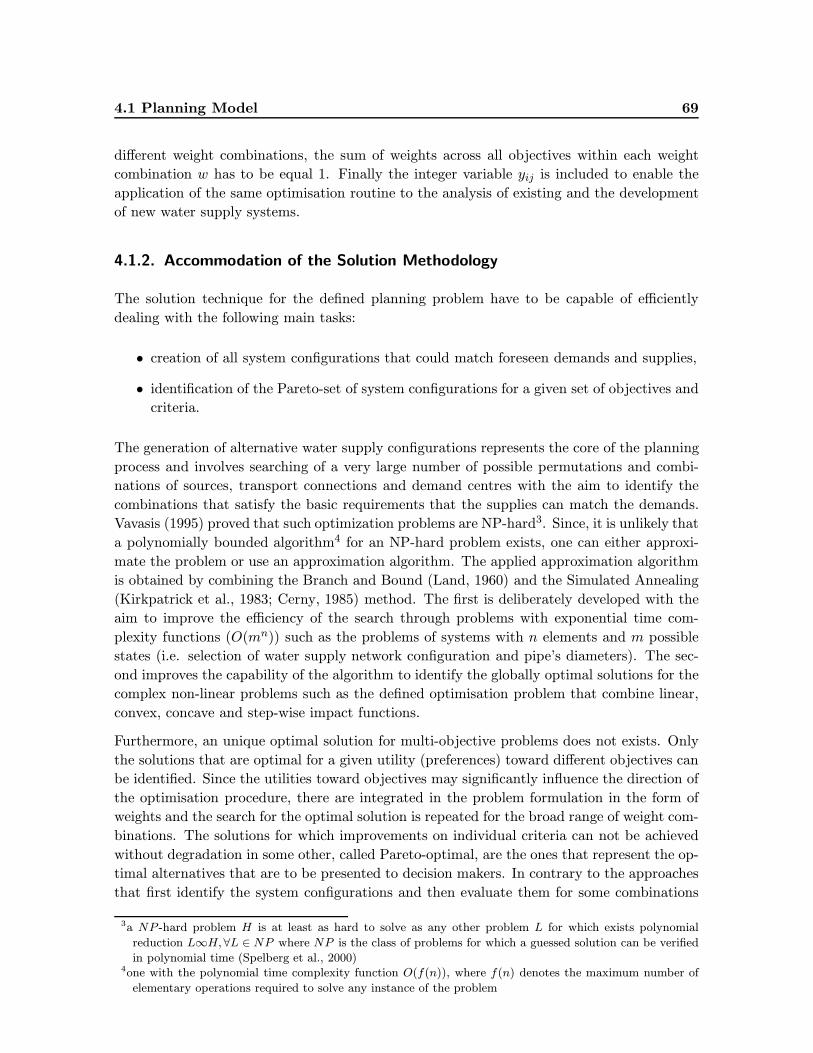
4.1 Planning Model 69
different weight combinations, the sum of weights across all objectives within each weight
combination w has to be equal 1. Finally the integer variable yij is included to enable the
application of the same optimisation routine to the analysis of existing and the development
of new water supply systems.
4.1.2. Accommodation of the Solution Methodology
The solution technique for the defined planning problem have to be capable of efficiently
dealing with the following main tasks:
• creation of all system configurations that could match foreseen demands and supplies,
• identification of the Pareto-set of system configurations for a given set of objectives and
criteria.
The generation of alternative water supply configurations represents the core of the planning
process and involves searching of a very large number of possible permutations and combi-
nations of sources, transport connections and demand centres with the aim to identify the
combinations that satisfy the basic requirements that the supplies can match the demands.
Vavasis (1995) proved that such optimization problems are NP-hard3. Since, it is unlikely that
a polynomially bounded algorithm4 for an NP-hard problem exists, one can either approxi-
mate the problem or use an approximation algorithm. The applied approximation algorithm
is obtained by combining the Branch and Bound (Land, 1960) and the Simulated Annealing
(Kirkpatrick et al., 1983; Cerny, 1985) method. The first is deliberately developed with the
aim to improve the efficiency of the search through problems with exponential time com-
plexity functions (O(mn)) such as the problems of systems with n elements and m possible
states (i.e. selection of water supply network configuration and pipe’s diameters). The sec-
ond improves the capability of the algorithm to identify the globally optimal solutions for the
complex non-linear problems such as the defined optimisation problem that combine linear,
convex, concave and step-wise impact functions.
Furthermore, an unique optimal solution for multi-objective problems does not exists. Only
the solutions that are optimal for a given utility (preferences) toward different objectives can
be identified. Since the utilities toward objectives may significantly influence the direction of
the optimisation procedure, there are integrated in the problem formulation in the form of
weights and the search for the optimal solution is repeated for the broad range of weight com-
binations. The solutions for which improvements on individual criteria can not be achieved
without degradation in some other, called Pareto-optimal, are the ones that represent the op-
timal alternatives that are to be presented to decision makers. In contrary to the approaches
that first identify the system configurations and then evaluate them for some combinations
3a NP -hard problem H is at least as hard to solve as any other problem L for which exists polynomial
reduction L∞H,∀L ∈ NP where NP is the class of problems for which a guessed solution can be verified
in polynomial time (Spelberg et al., 2000)4one with the polynomial time complexity function O(f(n)), where f(n) denotes the maximum number of
elementary operations required to solve any instance of the problem
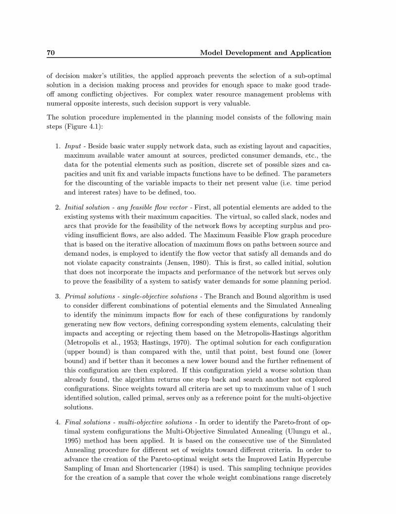
70 Model Development and Application
of decision maker’s utilities, the applied approach prevents the selection of a sub-optimal
solution in a decision making process and provides for enough space to make good trade-
off among conflicting objectives. For complex water resource management problems with
numeral opposite interests, such decision support is very valuable.
The solution procedure implemented in the planning model consists of the following main
steps (Figure 4.1):
1. Input - Beside basic water supply network data, such as existing layout and capacities,
maximum available water amount at sources, predicted consumer demands, etc., the
data for the potential elements such as position, discrete set of possible sizes and ca-
pacities and unit fix and variable impacts functions have to be defined. The parameters
for the discounting of the variable impacts to their net present value (i.e. time period
and interest rates) have to be defined, too.
2. Initial solution - any feasible flow vector - First, all potential elements are added to the
existing systems with their maximum capacities. The virtual, so called slack, nodes and
arcs that provide for the feasibility of the network flows by accepting surplus and pro-
viding insufficient flows, are also added. The Maximum Feasible Flow graph procedure
that is based on the iterative allocation of maximum flows on paths between source and
demand nodes, is employed to identify the flow vector that satisfy all demands and do
not violate capacity constraints (Jensen, 1980). This is first, so called initial, solution
that does not incorporate the impacts and performance of the network but serves only
to prove the feasibility of a system to satisfy water demands for some planning period.
3. Primal solutions - single-objective solutions - The Branch and Bound algorithm is used
to consider different combinations of potential elements and the Simulated Annealing
to identify the minimum impacts flow for each of these configurations by randomly
generating new flow vectors, defining corresponding system elements, calculating their
impacts and accepting or rejecting them based on the Metropolis-Hastings algorithm
(Metropolis et al., 1953; Hastings, 1970). The optimal solution for each configuration
(upper bound) is than compared with the, until that point, best found one (lower
bound) and if better than it becomes a new lower bound and the further refinement of
this configuration are then explored. If this configuration yield a worse solution than
already found, the algorithm returns one step back and search another not explored
configurations. Since weights toward all criteria are set up to maximum value of 1 such
identified solution, called primal, serves only as a reference point for the multi-objective
solutions.
4. Final solutions - multi-objective solutions - In order to identify the Pareto-front of op-
timal system configurations the Multi-Objective Simulated Annealing (Ulungu et al.,
1995) method has been applied. It is based on the consecutive use of the Simulated
Annealing procedure for different set of weights toward different criteria. In order to
advance the creation of the Pareto-optimal weight sets the Improved Latin Hypercube
Sampling of Iman and Shortencarier (1984) is used. This sampling technique provides
for the creation of a sample that cover the whole weight combinations range discretely
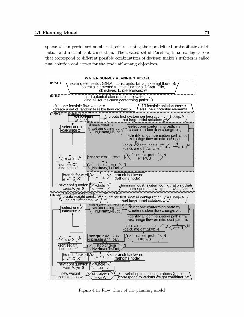
4.1 Planning Model 71
sparse with a predefined number of points keeping their predefined probabilistic distri-
bution and mutual rank correlation. The created set of Pareto-optimal configurations
that correspond to different possible combinations of decision maker’s utilities is called
final solution and serves for the trade-off among objectives.
Y
WATER SUPPLY PLANNING MODELexisting elements : G(N,A), constraints: kij, pij, external flows: Bij,
potential elements: yij, cost functions: DCvar, Cfix,objectives: L, preferences: wl
-find one feasible flow vector: x-create a set of random feasible flow vectors: X
INPUT:
-add potential elements to the system: yij-find all source-node conforming paths: Π
-create first system configuration: yij=1,∀aij∈A-set large initial solution: z=z’
-select one conforming path: πa-create random flow change: xπa
-identify all compensation paths: πci-exchange flow on min. cost path: πc
accept. prob.P=e∆z/BT
-set annealing par.T,N,Nmax,Nsucc
-calculate total costs: z‘‘-calculate diff ∆z=z‘‘-z‘
N
Y ∀π∈Π N
-accept: z‘=z‘‘, x‘=x‘‘-increase ann. par.
Y stop criteriaN>Nmax,T<Tmi
n
N
Y z’’< z N
-select one x’-calculate z’
Y ∀x∈X N
-sort set X’’-find best z’’
branch forwardz=z’’, X=X’’
branch backward(fathome node)
N wholetree
Ynew configuration∃aij∈A, yij=0
N all weights∀w∈W
Ynew weightcombination wl
set of optimal configurations X that correspond to various weight combinat. W
-create weight comb. W-select first comb. wl
INITIAL:
Y
-create first system configuration: yij=1,∀aij∈A-set large initial solution: z=z’
-select one conforming path: πa-create random flow change: xπa
-identify all compensation paths: πci-exchange flow on min. cost path:
πc
accept. prob.P=e∆z/BT
-set annealing par.T,N,Nmax,Nsucc
-calculate total costs: z‘‘-calculate diff ∆z=z‘‘-z‘
N
Y ∀π∈Π N
accept: z‘=z‘‘, x‘=x‘‘
Y stop criteriaN>Nmax,T<Tmi
n
N
Y z’’< z N
-select one x’-calculate z’
Y ∀x∈X N
-sort set X’’-find best z’’
branch forwardz=z’’, X=X’’
branch backward(fathome node)
N wholetree
Ynew configuration∃aij∈A, yij=0
minimum cost system configuration x that corresponds to weight set wl=1, ∀l∈L
set weightswl=1, ∀l∈L
PRIMAL: Branch & Bond
Simulated Annealing
If ∃ feasible solution then: xelse: new potential elements
FINAL: Branch & Bond
Multi-objective Simulated Annealing
Latin Hypercube Sampling
Figure 4.1.: Flow chart of the planning model
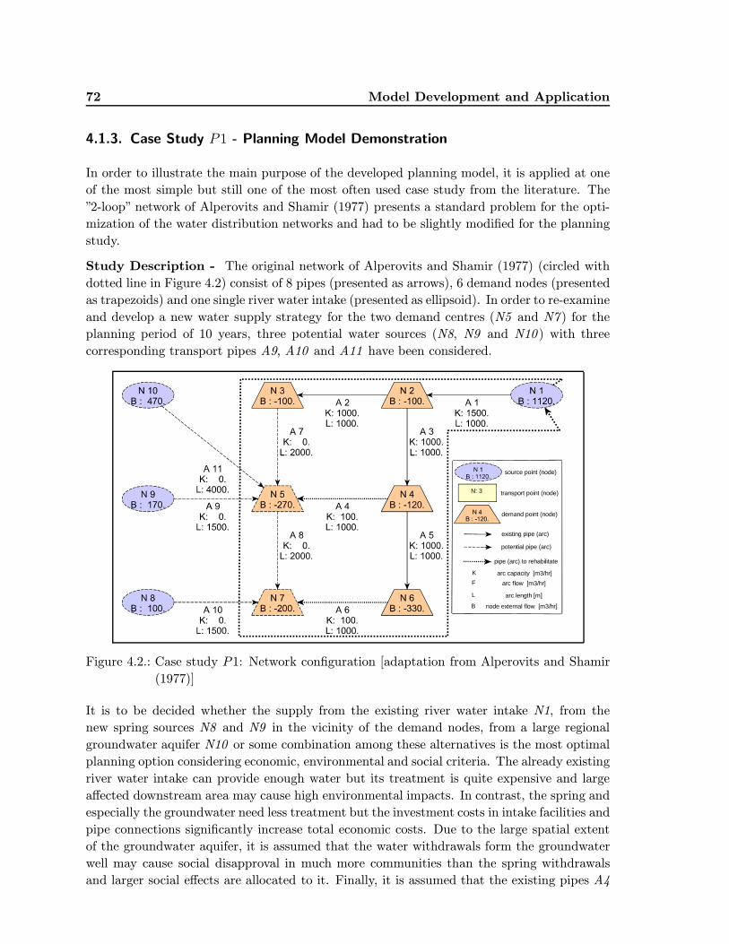
72 Model Development and Application
4.1.3. Case Study P1 - Planning Model Demonstration
In order to illustrate the main purpose of the developed planning model, it is applied at one
of the most simple but still one of the most often used case study from the literature. The
”2-loop” network of Alperovits and Shamir (1977) presents a standard problem for the opti-
mization of the water distribution networks and had to be slightly modified for the planning
study.
Study Description - The original network of Alperovits and Shamir (1977) (circled with
dotted line in Figure 4.2) consist of 8 pipes (presented as arrows), 6 demand nodes (presented
as trapezoids) and one single river water intake (presented as ellipsoid). In order to re-examine
and develop a new water supply strategy for the two demand centres (N5 and N7 ) for the
planning period of 10 years, three potential water sources (N8, N9 and N10 ) with three
corresponding transport pipes A9, A10 and A11 have been considered.
arc capacity [m3/hr]K
pipe (arc) to rehabilitate
potential pipe (arc)
existing pipe (arc)
demand point (node)
transport point (node)
source point (node)
N: 3
node external flow [m3/hr]B
arc flow [m3/hr]F
arc length [m]L
Figure 4.2.: Case study P1: Network configuration [adaptation from Alperovits and Shamir
(1977)]
It is to be decided whether the supply from the existing river water intake N1, from the
new spring sources N8 and N9 in the vicinity of the demand nodes, from a large regional
groundwater aquifer N10 or some combination among these alternatives is the most optimal
planning option considering economic, environmental and social criteria. The already existing
river water intake can provide enough water but its treatment is quite expensive and large
affected downstream area may cause high environmental impacts. In contrast, the spring and
especially the groundwater need less treatment but the investment costs in intake facilities and
pipe connections significantly increase total economic costs. Due to the large spatial extent
of the groundwater aquifer, it is assumed that the water withdrawals form the groundwater
well may cause social disapproval in much more communities than the spring withdrawals
and larger social effects are allocated to it. Finally, it is assumed that the existing pipes A4
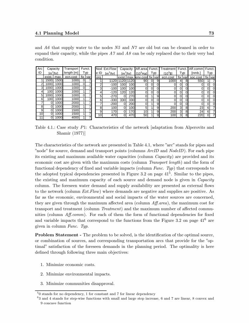
4.1 Planning Model 73
and A6 that supply water to the nodes N5 and N7 are old but can be cleaned in order to
expand their capacity, while the pipes A7 and A8 can be only replaced due to their very bad
condition.
Arc ID
Transport length [m]
exist. max. ecn.cost fix var1 1500 1500 1000 0 72 1000 1000 1000 0 73 1000 1000 1000 0 74 100 1000 1000 1 75 1000 1000 1000 0 76 100 1000 1000 1 77 0 1000 2000 1 78 0 1000 2000 1 79 0 1000 1500 1 7
10 0 1000 1500 1 711 0 1000 4000 1 7
Capacity
[m3/hr]
Funct. Typ
Node ID
Ext.Flow
[m3/hr]
Aff.area
[103Ha]
Treatment
[103$]
Aff.comm [nmb.]
org. exist. max. env.cost fix var ecn.cost fix var soc.cost fix var1 1120 1120 1120 90 0 9 1000 4 8 550 1 72 -100 100 100 0 0 0 0 0 0 0 0 03 -100 100 100 0 0 0 0 0 0 0 0 04 -120 120 120 0 0 0 0 0 0 0 0 05 -270 0 270 0 1 9 0 0 0 0 0 06 -330 330 330 0 0 0 0 0 0 0 0 07 -200 0 200 0 1 9 0 0 0 0 0 08 100 0 100 5 1 9 200 3 8 23 6 79 170 0 170 10 1 9 200 3 8 24 6 7
10 470 0 470 50 1 9 100 3 8 220 0 7
Capacity
[m3/hr]
Funct. Typ
Funct. Typ
Funct. Typ
Table 4.1.: Case study P1: Characteristics of the network [adaptation from Alperovits and
Shamir (1977)]
The characteristics of the network are presented in Table 4.1, where ”arc” stands for pipes and
”node” for source, demand and transport points (columns ArcID and NodeID). For each pipe
its existing and maximum available water capacities (column Capacity) are provided and its
economic cost are given with the maximum costs (column Transport length) and the form of
functional dependency of fixed and variable impacts (column Func. Typ) that corresponds to
the adopted typical dependencies presented in Figure 3.2 on page 415. Similar to the pipes,
the existing and maximum capacity of each source and demand node is given in Capacity
column. The foreseen water demand and supply availability are presented as external flows
to the network (column Ext.Flow) where demands are negative and supplies are positive. As
far as the economic, environmental and social impacts of the water sources are concerned,
they are given through the maximum affected area (column Aff.area), the maximum cost for
transport and treatment (column Treatment) and the maximum number of affected commu-
nities (column Aff.comm). For each of them the form of functional dependencies for fixed
and variable impacts that correspond to the functions from the Figure 3.2 on page 416 are
given in column Func. Typ.
Problem Statement - The problem to be solved, is the identification of the optimal source,
or combination of sources, and corresponding transportation arcs that provide for the ”op-
timal” satisfaction of the foreseen demands in the planning period. The optimality is here
defined through following three main objectives:
1. Minimize economic costs.
2. Minimize environmental impacts.
3. Minimize communities disapproval.
50 stands for no dependency, 1 for constant and 7 for linear dependency63 and 4 stands for step-wise functions with small and large step increase, 6 and 7 are linear, 8 convex and
9 concave function
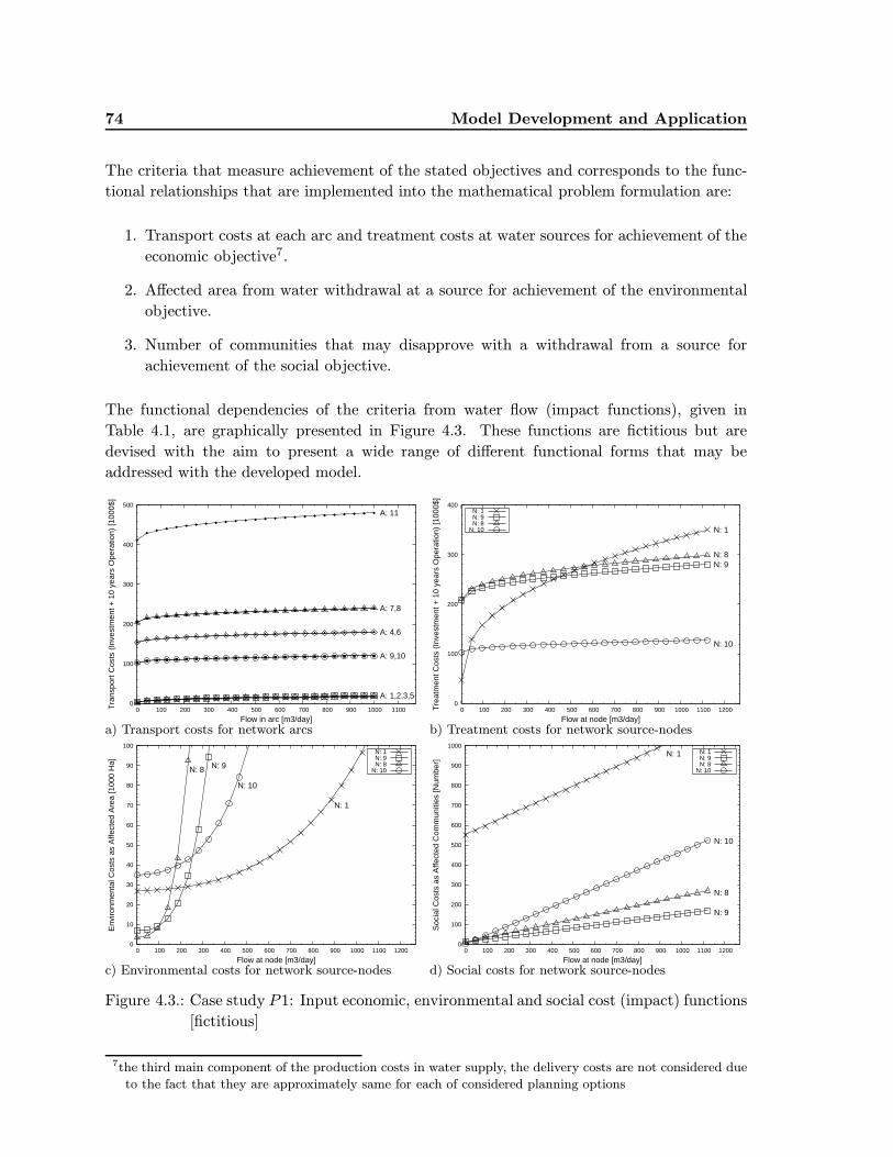
74 Model Development and Application
The criteria that measure achievement of the stated objectives and corresponds to the func-
tional relationships that are implemented into the mathematical problem formulation are:
1. Transport costs at each arc and treatment costs at water sources for achievement of the
economic objective7.
2. Affected area from water withdrawal at a source for achievement of the environmental
objective.
3. Number of communities that may disapprove with a withdrawal from a source for
achievement of the social objective.
The functional dependencies of the criteria from water flow (impact functions), given in
Table 4.1, are graphically presented in Figure 4.3. These functions are fictitious but are
devised with the aim to present a wide range of different functional forms that may be
addressed with the developed model.
0
100
200
300
400
500
0 100 200 300 400 500 600 700 800 900 1000 1100Tra
nspo
rt C
osts
(In
vest
men
t + 1
0 ye
ars
Ope
ratio
n) [1
000$
]
Flow in arc [m3/day]
A: 1,2,3,5
A: 4,6
A: 7,8
A: 9,10
A: 11
a) Transport costs for network arcs
0
100
200
300
400
0 100 200 300 400 500 600 700 800 900 1000 1100 1200Tre
atm
ent C
osts
(In
vest
men
t + 1
0 ye
ars
Ope
ratio
n) [1
000$
]
Flow at node [m3/day]
N: 1
N: 9N: 8
N: 10
N: 1N: 9N: 8
N: 10
b) Treatment costs for network source-nodes
0
10
20
30
40
50
60
70
80
90
100
0 100 200 300 400 500 600 700 800 900 1000 1100 1200
Env
ironm
enta
l Cos
ts a
s A
ffect
ed A
rea
[100
0 H
a]
Flow at node [m3/day]
N: 1
N: 9N: 8
N: 10
N: 1N: 9N: 8
N: 10
c) Environmental costs for network source-nodes
0
100
200
300
400
500
600
700
800
900
1000
0 100 200 300 400 500 600 700 800 900 1000 1100 1200
Soc
ial C
osts
as
Affe
cted
Com
mun
ities
[Num
ber]
Flow at node [m3/day]
N: 1
N: 9
N: 8
N: 10
N: 1N: 9N: 8
N: 10
d) Social costs for network source-nodes
Figure 4.3.: Case study P1: Input economic, environmental and social cost (impact) functions
[fictitious]
7the third main component of the production costs in water supply, the delivery costs are not considered due
to the fact that they are approximately same for each of considered planning options

4.1 Planning Model 75
As it can be seen in graph a in Figure 4.3 the operation cost for all pipes are devised as
concave functions in order to imitate the ”economy of scale” effect. The main economic
difference among individual transport pipes comes from the investment costs, which differs
from relatively small, for the transport from nearby spring sources (A10,A9 ), a bit larger for
the rehabilitation of the existing arcs (A4,A6 ), proportionally larger for the new arcs (A7,A8 )
and very large for the building of new connection (A11 ) to the remote regional groundwater
aquifer. For the treatment costs (graph b in Figure 4.3) the effect of ”economy of scale” is even
more present since the investment costs have the same order of magnitude as the operation
costs for the adopted planning period of 10 years. For example, although the opening of the
new sources (N8,N9 and N10 ) has larger investment costs than the expansion of the already
existing river water intake (N1 ), for river withdrawal amounts larger then 50 m3/day and
500 m3/day, the costs of the river water treatment become larger than the investment and
operation costs in the new groundwater well and in the new spring sources, respectively.
The environmental impacts of the water withdrawal from different sources (graph c in Fig-
ure 4.3) are devised in a way that the initially affected areas from the groundwater (N10) and
river water (N1 ) intakes are significantly larger than the ones from the springs (N9, N8 ). Still
due to the very small capacity of the springs their negative environmental impacts progress
much more rapidly than for the first two sources. Such exponential dependencies are quite
typical for environmental impacts.
Finally the social effects of water withdrawal from some node are presented as linear functions.
Due to the already quite large river water use and quite large affected downstream area, many
communities are a priory against further expansion of this source (large initial value for line
N1 graph d in Figure 4.3). Although initially there is no opposition for the use of groundwater
(N10 ), it is assumed that the large use of this strategically important water resources may
on a long term cause much larger social discrepancies than the other ones and the largest
slope has been allocated to this function. Since there are only a few communities that are
affected by the use of water from spring intakes N9, N8 their social impacts are quite small.
Finally it has to be underlined again that, although these dependencies aim to imitate the
often found conditions in real water supply systems, they are purely fictitious and produced
only for the purpose of the illustration of the capabilities of the planning model.
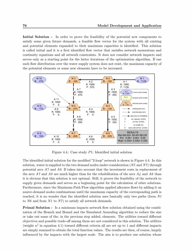
76 Model Development and Application
Initial Solution - In order to prove the feasibility of the potential new components to
satisfy some given future demands, a feasible flow vector for the system with all existing
and potential elements expanded to their maximum capacities is identified. This solution
is called initial and it is a first identified flow vector that satisfies network momentum and
continuity equations and all network constraints. It does not consider network impacts and
serves only as a starting point for the latter iterations of the optimisation algorithm. If one
such flow distribution over the water supply system does not exist, the maximum capacity of
the potential elements or some new elements have to be increased.
arc capacity [m3/hr]K
pipe (arc) to rehabilitate
potential pipe (arc)
existing pipe (arc)
demand point (node)
transport point (node)
source point (node)
N: 3
node external flow [m3/hr]B
arc flow [m3/hr]F
arc length [m]L
Figure 4.4.: Case study P1: Identified initial solution
The identified initial solution for the modified ”2-loop” network is shown in Figure 4.4. In this
solution, water is supplied to the two demand nodes under consideration (N5 and N7 ) through
potential arcs A7 and A8. If taken into account that the investment costs in replacement of
the arcs A7 and A8 are much higher than for the rehabilitation of the arcs A4 and A6 than
it is obvious that this solution is not optimal. Still, it proves the feasibility of the network to
supply given demands and serves as a beginning point for the calculation of other solutions.
Furthermore, since the Maximum Path Flow algorithm applied allocates flows by adding it on
source-demand nodes combinations until the maximum capacity of the corresponding path is
reached, it is no wonder that the identified solution uses basically only two paths (form N1
to N6 and from N1 to N7 ) to satisfy all network demands.
Primal Solution - Is a minimum impacts network flow solution obtained using the combi-
nation of the Branch and Bound and the Simulated Annealing algorithm to reduce the size
or take out some of the, in the previous step added, elements. The utilities toward different
objectives and possible trade-off among them are not considered in this solution. The utilities
(weight wl in equation 4.1) toward different criteria all are set up to 1 and different impacts
are simply summed to obtain the total function values. The results are then, of course, largely
influenced by the impacts with the largest scale. The aim is to produce one solution whose
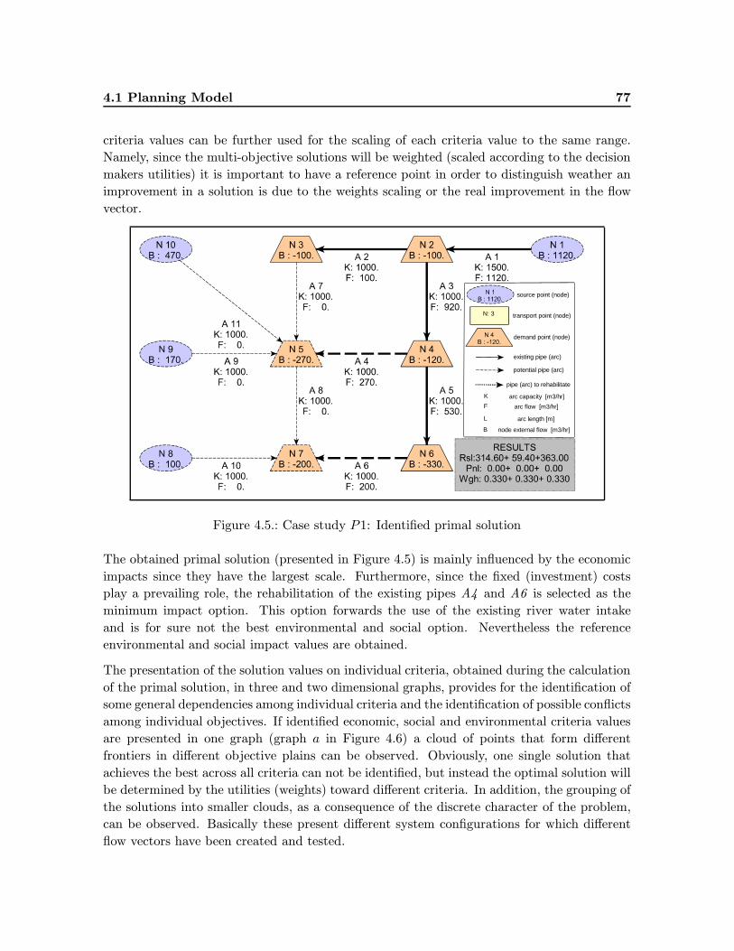
4.1 Planning Model 77
criteria values can be further used for the scaling of each criteria value to the same range.
Namely, since the multi-objective solutions will be weighted (scaled according to the decision
makers utilities) it is important to have a reference point in order to distinguish weather an
improvement in a solution is due to the weights scaling or the real improvement in the flow
vector.
arc capacity [m3/hr]K
pipe (arc) to rehabilitate
potential pipe (arc)
existing pipe (arc)
demand point (node)
transport point (node)
source point (node)
N: 3
node external flow [m3/hr]B
arc flow [m3/hr]F
arc length [m]L
Figure 4.5.: Case study P1: Identified primal solution
The obtained primal solution (presented in Figure 4.5) is mainly influenced by the economic
impacts since they have the largest scale. Furthermore, since the fixed (investment) costs
play a prevailing role, the rehabilitation of the existing pipes A4 and A6 is selected as the
minimum impact option. This option forwards the use of the existing river water intake
and is for sure not the best environmental and social option. Nevertheless the reference
environmental and social impact values are obtained.
The presentation of the solution values on individual criteria, obtained during the calculation
of the primal solution, in three and two dimensional graphs, provides for the identification of
some general dependencies among individual criteria and the identification of possible conflicts
among individual objectives. If identified economic, social and environmental criteria values
are presented in one graph (graph a in Figure 4.6) a cloud of points that form different
frontiers in different objective plains can be observed. Obviously, one single solution that
achieves the best across all criteria can not be identified, but instead the optimal solution will
be determined by the utilities (weights) toward different criteria. In addition, the grouping of
the solutions into smaller clouds, as a consequence of the discrete character of the problem,
can be observed. Basically these present different system configurations for which different
flow vectors have been created and tested.
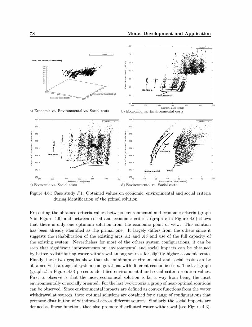
78 Model Development and Application
200 300
400 500
600 700
800 45 50
55 60
65 70
75 80
320 330 340 350 360 370 380 390 400
Socio Costs [Number of Communities]
solution
Economic Costs [1000$]
Environmental Costs [1000Ha]
Socio Costs [Number of Communities]
a) Economic vs. Environmental vs. Social costs
45
50
55
60
65
70
75
80
200 300 400 500 600 700 800
Env
ironm
enta
l Cos
ts [1
000H
a]
Economic Costs [1000$]
solution
economic
environmental
b) Economic vs. Environmental costs
340
345
350
355
360
365
370
375
380
200 300 400 500 600 700 800
Soc
io C
osts
[Num
ber
of C
omm
uniti
es]
Economic Costs [1000$]
solution
economic
socio
c) Economic vs. Social costs
340
345
350
355
360
365
370
375
380
45 50 55 60 65 70 75 80
Soc
io C
osts
[Num
ber
of C
omm
uniti
es]
Environmental Costs [1000Ha]
solution
economic
environmental socio
d) Environmental vs. Social costs
Figure 4.6.: Case study P1: Obtained values on economic, environmental and social criteria
during identification of the primal solution
Presenting the obtained criteria values between environmental and economic criteria (graph
b in Figure 4.6) and between social and economic criteria (graph c in Figure 4.6) shows
that there is only one optimum solution from the economic point of view. This solution
has been already identified as the primal one. It largely differs from the others since it
suggests the rehabilitation of the existing arcs A4 and A6 and use of the full capacity of
the existing system. Nevertheless for most of the others system configurations, it can be
seen that significant improvements on environmental and social impacts can be obtained
by better redistributing water withdrawal among sources for slightly higher economic costs.
Finally these two graphs show that the minimum environmental and social costs can be
obtained with a range of system configurations with different economic costs. The last graph
(graph d in Figure 4.6) presents identified environmental and social criteria solution values.
First to observe is that the most economical solution is far a way from being the most
environmentally or socially oriented. For the last two criteria a group of near-optimal solutions
can be observed. Since environmental impacts are defined as convex functions from the water
withdrawal at sources, these optimal solutions are obtained for a range of configurations that
promote distribution of withdrawal across different sources. Similarly the social impacts are
defined as linear functions that also promote distributed water withdrawal (see Figure 4.3).
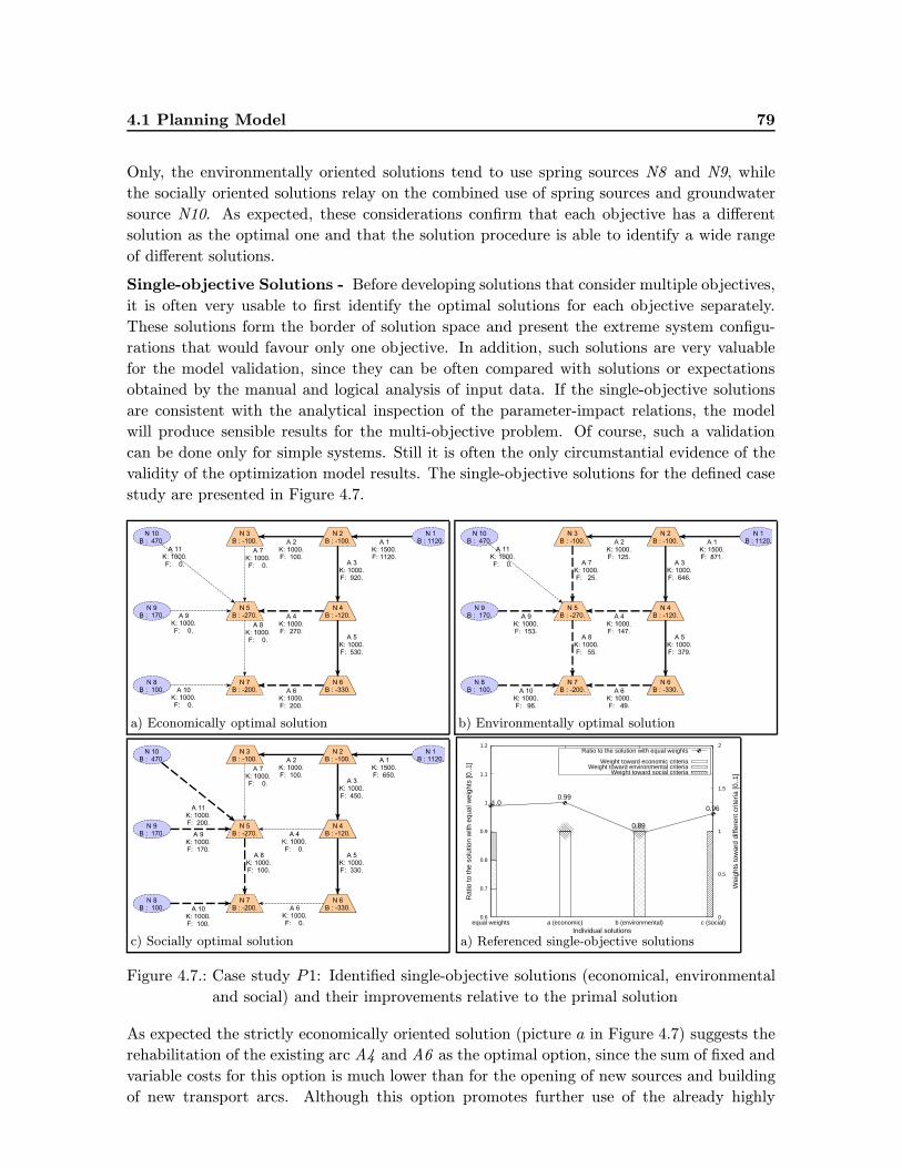
4.1 Planning Model 79
Only, the environmentally oriented solutions tend to use spring sources N8 and N9, while
the socially oriented solutions relay on the combined use of spring sources and groundwater
source N10. As expected, these considerations confirm that each objective has a different
solution as the optimal one and that the solution procedure is able to identify a wide range
of different solutions.
Single-objective Solutions - Before developing solutions that consider multiple objectives,
it is often very usable to first identify the optimal solutions for each objective separately.
These solutions form the border of solution space and present the extreme system configu-
rations that would favour only one objective. In addition, such solutions are very valuable
for the model validation, since they can be often compared with solutions or expectations
obtained by the manual and logical analysis of input data. If the single-objective solutions
are consistent with the analytical inspection of the parameter-impact relations, the model
will produce sensible results for the multi-objective problem. Of course, such a validation
can be done only for simple systems. Still it is often the only circumstantial evidence of the
validity of the optimization model results. The single-objective solutions for the defined case
study are presented in Figure 4.7.
a) Economically optimal solution
b) Environmentally optimal solution
c) Socially optimal solution
0.6
0.7
0.8
0.9
1
1.1
1.2
equal weights a (economic) b (environmental) c (social) 0
0.5
1
1.5
2
Rat
io to
the
solu
tion
with
equ
al w
eigh
ts [0
..1]
Wei
ghts
tow
ard
diffe
rent
crit
eria
[0..1
]
Individual solutions
1.00.99
0.89
0.96
Ratio to the solution with equal weights
Weight toward economic criteriaWeight toward environmental criteria
Weight toward social criteria
a) Referenced single-objective solutions
Figure 4.7.: Case study P1: Identified single-objective solutions (economical, environmental
and social) and their improvements relative to the primal solution
As expected the strictly economically oriented solution (picture a in Figure 4.7) suggests the
rehabilitation of the existing arc A4 and A6 as the optimal option, since the sum of fixed and
variable costs for this option is much lower than for the opening of new sources and building
of new transport arcs. Although this option promotes further use of the already highly
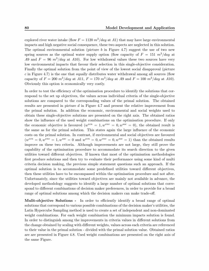
80 Model Development and Application
explored river water intake (flow F = 1120 m3/day at A1) that may have large environmental
impacts and high negative social consequence, these two aspects are neglected in this solution.
The optimal environmental solution (picture b in Figure 4.7) suggest the use of two new
spring sources as the optimal water supply option (flow capacity of F = 151 m3/day at
A9 and F = 96 m3/day at A10). For low withdrawal values these two sources have very
low environmental impacts that favour their selection in this single-objective consideration.
Finally the optimal solution from the point of view of the lowest social disapproval (picture
c in Figure 4.7) is the one that equally distributes water withdrawal among all sources (flow
capacity of F = 200 m3/day at A11, F = 170 m3/day at A9 and F = 100 m3/day at A10).
Obviously this option is economically very costly.
In order to test the efficiency of the optimisation procedure to identify the solutions that cor-
respond to the set up objectives, the values across individual criteria of the single-objective
solutions are compared to the corresponding values of the primal solution. The obtained
results are presented in picture d in Figure 4.7 and present the relative improvement from
the primal solution. In addition the economic, environmental and social weights used to
obtain these single-objective solutions are presented on the right axis. The obtained ratios
show the influence of the used weight combinations on the optimisation procedure. If only
the economic objective is favoured (wecn = 1, wenv = 0, wsoc = 0), the obtained result is
the same as for the primal solution. This states again the large influence of the economic
costs on the primal solution. In contrast, if environmental and social objectives are favoured
(wecn = 0, wenv = 1, wsoc = 0 and wecn = 0, wenv = 0, wsoc = 1) than the obtained results
improve on these two criteria. Although improvements are not large, they still prove the
capability of the optimisation procedure to accommodate its search direction to the given
utilities toward different objectives. If known that most of the optimisation methodologies
first produce solutions and then try to evaluate their performance using some kind of multi
criteria decision making, the previous simple statement questions such an approach. If the
optimal solution is to accommodate some predefined utilities toward different objectives,
then these utilities have to be encompassed within the optimisation procedure and not after.
Unfortunately, since the utilities toward objectives are mainly not available in advance, the
developed methodology suggests to identify a large number of optimal solutions that corre-
spond to different combinations of decision maker preferences, in order to provide for a broad
range of optimal solutions among which the decision makers can make trade-off.
Mulit-objective Solutions - In order to efficiently identify a broad range of optimal
solutions that correspond to various possible combinations of the decision maker’s utilities, the
Latin Hypercube Sampling method is used to create a set of independent and non-dominated
weight combinations. For each weight combination the minimum impacts solution is found.
In order to distinguish among the improvements in criteria values in different solutions from
the change obtained by scaling with different weights, values across each criteria are referenced
to their value in the primal solution - divided with the primal solution value. Obtained ratios
are are presented in Figure 4.8. Used weight combinations are presented on the right axis of
the same Figure.
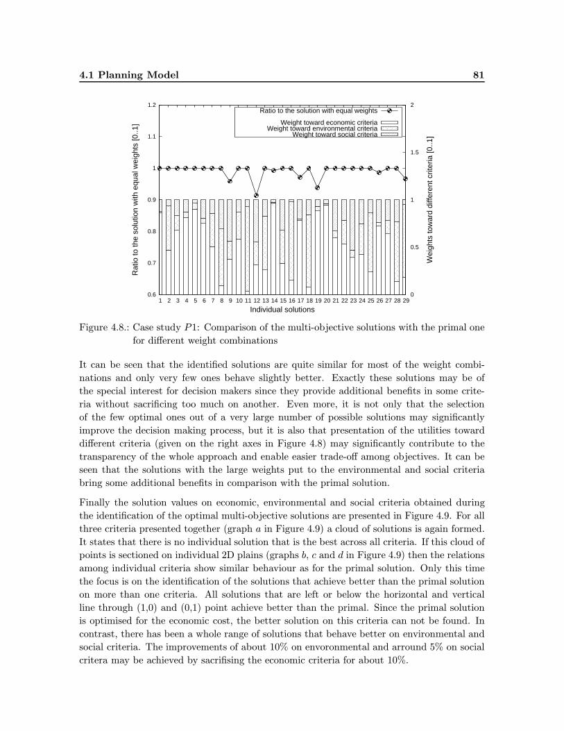
4.1 Planning Model 81
0.6
0.7
0.8
0.9
1
1.1
1.2
1 2 3 4 5 6 7 8 9 10 11 12 13 14 15 16 17 18 19 20 21 22 23 24 25 26 27 28 29 0
0.5
1
1.5
2
Rat
io to
the
solu
tion
with
equ
al w
eigh
ts [0
..1]
Wei
ghts
tow
ard
diffe
rent
crit
eria
[0..1
]
Individual solutions
Ratio to the solution with equal weights
Weight toward economic criteriaWeight toward environmental criteria
Weight toward social criteria
Figure 4.8.: Case study P1: Comparison of the multi-objective solutions with the primal one
for different weight combinations
It can be seen that the identified solutions are quite similar for most of the weight combi-
nations and only very few ones behave slightly better. Exactly these solutions may be of
the special interest for decision makers since they provide additional benefits in some crite-
ria without sacrificing too much on another. Even more, it is not only that the selection
of the few optimal ones out of a very large number of possible solutions may significantly
improve the decision making process, but it is also that presentation of the utilities toward
different criteria (given on the right axes in Figure 4.8) may significantly contribute to the
transparency of the whole approach and enable easier trade-off among objectives. It can be
seen that the solutions with the large weights put to the environmental and social criteria
bring some additional benefits in comparison with the primal solution.
Finally the solution values on economic, environmental and social criteria obtained during
the identification of the optimal multi-objective solutions are presented in Figure 4.9. For all
three criteria presented together (graph a in Figure 4.9) a cloud of solutions is again formed.
It states that there is no individual solution that is the best across all criteria. If this cloud of
points is sectioned on individual 2D plains (graphs b, c and d in Figure 4.9) then the relations
among individual criteria show similar behaviour as for the primal solution. Only this time
the focus is on the identification of the solutions that achieve better than the primal solution
on more than one criteria. All solutions that are left or below the horizontal and vertical
line through (1,0) and (0,1) point achieve better than the primal. Since the primal solution
is optimised for the economic cost, the better solution on this criteria can not be found. In
contrast, there has been a whole range of solutions that behave better on environmental and
social criteria. The improvements of about 10% on envoronmental and arround 5% on social
critera may be achieved by sacrifising the economic criteria for about 10%.
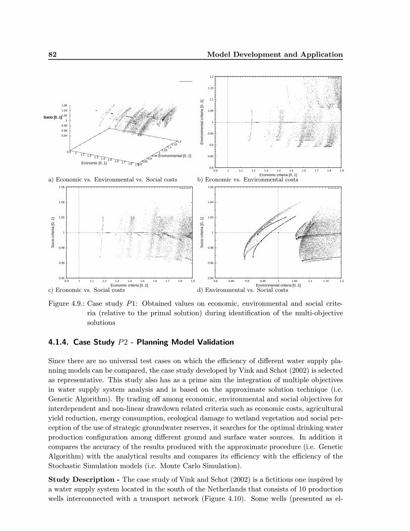
82 Model Development and Application
0.9 1 1.1 1.2 1.3 1.4 1.5 1.6 1.7 1.8 1.9 0.8 0.85
0.9 0.95
1 1.05
1.1 1.15
1.2
0.94
0.96
0.98
1
1.02
1.04
1.06
Socio [0..1]
Economic [0..1]
Environmental [0..1]
Socio [0..1]
a) Economic vs. Environmental vs. Social costs
0.8
0.85
0.9
0.95
1
1.05
1.1
1.15
1.2
0.9 1 1.1 1.2 1.3 1.4 1.5 1.6 1.7 1.8 1.9
Env
ironm
enta
l crit
eria
[0..1
]
Economic criteria [0..1]b) Economic vs. Environmental costs
0.94
0.96
0.98
1
1.02
1.04
1.06
0.9 1 1.1 1.2 1.3 1.4 1.5 1.6 1.7 1.8 1.9
Soc
io c
riter
ia [0
..1]
Economic criteria [0..1]c) Economic vs. Social costs
0.94
0.96
0.98
1
1.02
1.04
1.06
0.8 0.85 0.9 0.95 1 1.05 1.1 1.15 1.2
Soc
io c
riter
ia [0
..1]
Environmental criteria [0..1]d) Environmental vs. Social costs
Figure 4.9.: Case study P1: Obtained values on economic, environmental and social crite-
ria (relative to the primal solution) during identification of the multi-objective
solutions
4.1.4. Case Study P2 - Planning Model Validation
Since there are no universal test cases on which the efficiency of different water supply pla-
nning models can be compared, the case study developed by Vink and Schot (2002) is selected
as representative. This study also has as a prime aim the integration of multiple objectives
in water supply system analysis and is based on the approximate solution technique (i.e.
Genetic Algorithm). By trading off among economic, environmental and social objectives for
interdependent and non-linear drawdown related criteria such as economic costs, agricultural
yield reduction, energy consumption, ecological damage to wetland vegetation and social per-
ception of the use of strategic groundwater reserves, it searches for the optimal drinking water
production configuration among different ground and surface water sources. In addition it
compares the accuracy of the results produced with the approximate procedure (i.e. Genetic
Algorithm) with the analytical results and compares its efficiency with the efficiency of the
Stochastic Simulation models (i.e. Monte Carlo Simulation).
Study Description - The case study of Vink and Schot (2002) is a fictitious one inspired by
a water supply system located in the south of the Netherlands that consists of 10 production
wells interconnected with a transport network (Figure 4.10). Some wells (presented as el-
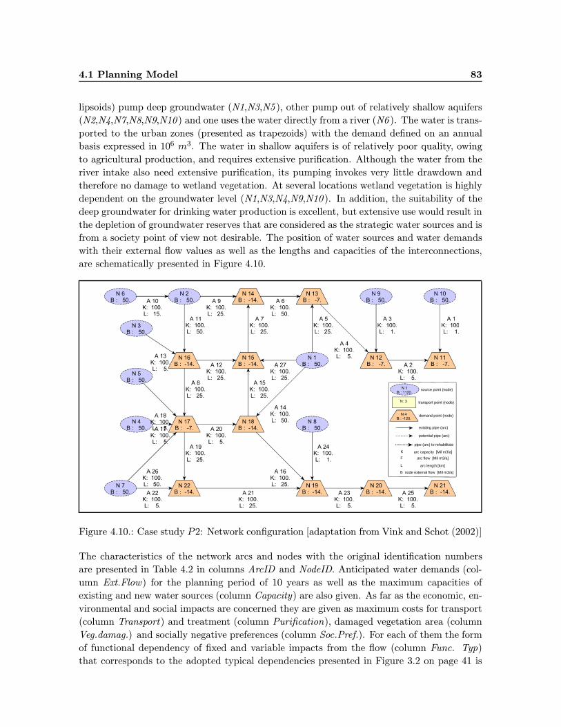
4.1 Planning Model 83
lipsoids) pump deep groundwater (N1,N3,N5 ), other pump out of relatively shallow aquifers
(N2,N4,N7,N8,N9,N10 ) and one uses the water directly from a river (N6 ). The water is trans-
ported to the urban zones (presented as trapezoids) with the demand defined on an annual
basis expressed in 106 m3. The water in shallow aquifers is of relatively poor quality, owing
to agricultural production, and requires extensive purification. Although the water from the
river intake also need extensive purification, its pumping invokes very little drawdown and
therefore no damage to wetland vegetation. At several locations wetland vegetation is highly
dependent on the groundwater level (N1,N3,N4,N9,N10 ). In addition, the suitability of the
deep groundwater for drinking water production is excellent, but extensive use would result in
the depletion of groundwater reserves that are considered as the strategic water sources and is
from a society point of view not desirable. The position of water sources and water demands
with their external flow values as well as the lengths and capacities of the interconnections,
are schematically presented in Figure 4.10.
arc capacity [Mil m3/a]K
pipe (arc) to rehabilitate
potential pipe (arc)
existing pipe (arc)
demand point (node)
transport point (node)
source point (node)
N: 3
node external flow [Mil m3/a]B
arc flow [Mil m3/a]F
arc length [km]L
Figure 4.10.: Case study P2: Network configuration [adaptation from Vink and Schot (2002)]
The characteristics of the network arcs and nodes with the original identification numbers
are presented in Table 4.2 in columns ArcID and NodeID. Anticipated water demands (col-
umn Ext.Flow) for the planning period of 10 years as well as the maximum capacities of
existing and new water sources (column Capacity) are also given. As far as the economic, en-
vironmental and social impacts are concerned they are given as maximum costs for transport
(column Transport) and treatment (column Purification), damaged vegetation area (column
Veg.damag.) and socially negative preferences (column Soc.Pref.). For each of them the form
of functional dependency of fixed and variable impacts from the flow (column Func. Typ)
that corresponds to the adopted typical dependencies presented in Figure 3.2 on page 41 is
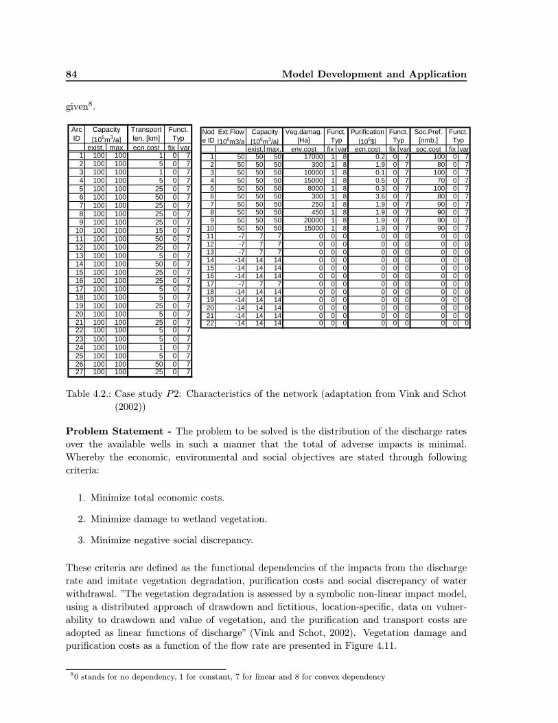
84 Model Development and Application
given8.
Arc ID
Transport len. [km]
exist. max. ecn.cost fix var1 100 100 1 0 72 100 100 5 0 73 100 100 1 0 74 100 100 5 0 75 100 100 25 0 76 100 100 50 0 77 100 100 25 0 78 100 100 25 0 79 100 100 25 0 7
10 100 100 15 0 711 100 100 50 0 712 100 100 25 0 713 100 100 5 0 714 100 100 50 0 715 100 100 25 0 716 100 100 25 0 717 100 100 5 0 718 100 100 5 0 719 100 100 25 0 720 100 100 5 0 721 100 100 25 0 722 100 100 5 0 723 100 100 5 0 724 100 100 1 0 725 100 100 5 0 726 100 100 50 0 727 100 100 25 0 7
Capacity
[106m3/a]
Funct. Typ
Node ID
Ext.Flow
[106m3/a
Veg.damag. [Ha]
Purification
[106$]
Soc.Pref. [nmb.]
exist. max. env.cost fix var ecn.cost fix var soc.cost fix var1 50 50 50 17000 1 8 0.2 0 7 100 0 72 50 50 50 300 1 8 1.9 0 7 80 0 73 50 50 50 10000 1 8 0.1 0 7 100 0 74 50 50 50 15000 1 8 0.5 0 7 70 0 75 50 50 50 8000 1 8 0.3 0 7 100 0 76 50 50 50 300 1 8 3.6 0 7 80 0 77 50 50 50 250 1 8 1.9 0 7 90 0 78 50 50 50 450 1 8 1.9 0 7 90 0 79 50 50 50 20000 1 8 1.9 0 7 90 0 7
10 50 50 50 15000 1 8 1.9 0 7 90 0 711 -7 7 7 0 0 0 0 0 0 0 0 012 -7 7 7 0 0 0 0 0 0 0 0 013 -7 7 7 0 0 0 0 0 0 0 0 014 -14 14 14 0 0 0 0 0 0 0 0 015 -14 14 14 0 0 0 0 0 0 0 0 016 -14 14 14 0 0 0 0 0 0 0 0 017 -7 7 7 0 0 0 0 0 0 0 0 018 -14 14 14 0 0 0 0 0 0 0 0 019 -14 14 14 0 0 0 0 0 0 0 0 020 -14 14 14 0 0 0 0 0 0 0 0 021 -14 14 14 0 0 0 0 0 0 0 0 022 -14 14 14 0 0 0 0 0 0 0 0 0
Capacity
[106m3/a]
Funct. Typ
Funct. Typ
Funct. Typ
Table 4.2.: Case study P2: Characteristics of the network (adaptation from Vink and Schot
(2002))
Problem Statement - The problem to be solved is the distribution of the discharge rates
over the available wells in such a manner that the total of adverse impacts is minimal.
Whereby the economic, environmental and social objectives are stated through following
criteria:
1. Minimize total economic costs.
2. Minimize damage to wetland vegetation.
3. Minimize negative social discrepancy.
These criteria are defined as the functional dependencies of the impacts from the discharge
rate and imitate vegetation degradation, purification costs and social discrepancy of water
withdrawal. ”The vegetation degradation is assessed by a symbolic non-linear impact model,
using a distributed approach of drawdown and fictitious, location-specific, data on vulner-
ability to drawdown and value of vegetation, and the purification and transport costs are
adopted as linear functions of discharge” (Vink and Schot, 2002). Vegetation damage and
purification costs as a function of the flow rate are presented in Figure 4.11.
80 stands for no dependency, 1 for constant, 7 for linear and 8 for convex dependency
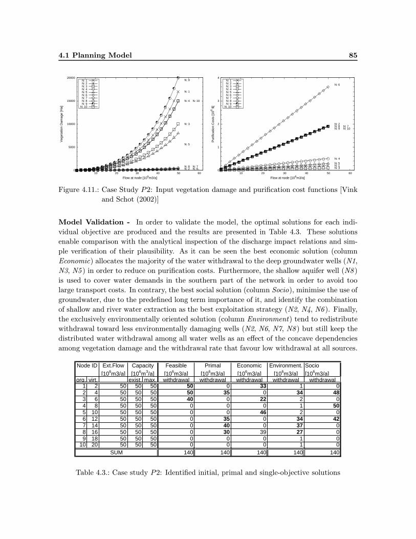
4.1 Planning Model 85
0
5000
10000
15000
20000
10 20 30 40 50 60
Veg
etat
ion
Dam
age
[Ha]
Flow at node [106m3/a]
N: 1
N: 2
N: 3
N: 4
N: 5
N: 6N: 7N: 8
N: 9
N: 10
N: 1N: 2N: 3N: 4N: 5N: 6N: 7N: 8N: 9
N: 10
0
1
2
3
4
10 20 30 40 50 60
Pur
ifica
tion
Cos
ts [1
06 $]
Flow at node [106m3/a]
N: 1
N: 2
N: 3
N: 4
N: 5
N: 6
N: 7N: 8N: 9 N: 10
N: 1N: 2N: 3N: 4N: 5N: 6N: 7N: 8N: 9
N: 10
Figure 4.11.: Case Study P2: Input vegetation damage and purification cost functions [Vink
and Schot (2002)]
Model Validation - In order to validate the model, the optimal solutions for each indi-
vidual objective are produced and the results are presented in Table 4.3. These solutions
enable comparison with the analytical inspection of the discharge impact relations and sim-
ple verification of their plausibility. As it can be seen the best economic solution (column
Economic) allocates the majority of the water withdrawal to the deep groundwater wells (N1,
N3, N5 ) in order to reduce on purification costs. Furthermore, the shallow aquifer well (N8 )
is used to cover water demands in the southern part of the network in order to avoid too
large transport costs. In contrary, the best social solution (column Socio), minimise the use of
groundwater, due to the predefined long term importance of it, and identify the combination
of shallow and river water extraction as the best exploitation strategy (N2, N4, N6 ). Finally,
the exclusively environmentally oriented solution (column Environment) tend to redistribute
withdrawal toward less environmentally damaging wells (N2, N6, N7, N8 ) but still keep the
distributed water withdrawal among all water wells as an effect of the concave dependencies
among vegetation damage and the withdrawal rate that favour low withdrawal at all sources.
Ext.Flow
[106m3/a]
Feasible
[106m3/a]
Primal
[106m3/a]
Economic
[106m3/a]
Environment.
[106m3/a]
Socio
[106m3/a]org. virt. exist. max. withdrawal withdrawal withdrawal withdrawal withdrawal
1 2 50 50 50 50 0 33 1 02 4 50 50 50 50 35 0 34 483 6 50 50 50 40 0 22 2 04 8 50 50 50 0 0 0 1 505 10 50 50 50 0 0 46 2 06 12 50 50 50 0 35 0 34 427 14 50 50 50 0 40 0 37 08 16 50 50 50 0 30 39 27 09 18 50 50 50 0 0 0 1 0
10 20 50 50 50 0 0 0 1 0140 140 140 140 140
Capacity
[106m3/a]
SUM
Node ID
Table 4.3.: Case study P2: Identified initial, primal and single-objective solutions
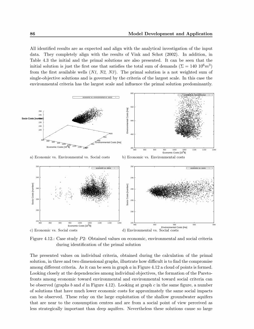
86 Model Development and Application
All identified results are as expected and align with the analytical investigation of the input
data. They completely align with the results of Vink and Schot (2002). In addition, in
Table 4.3 the initial and the primal solutions are also presented. It can be seen that the
initial solution is just the first one that satisfies the total sum of demands (Σ = 140 106m3)
from the first available wells (N1, N2, N3 ). The primal solution is a not weighted sum of
single-objective solutions and is governed by the criteria of the largest scale. In this case the
environmental criteria has the largest scale and influence the primal solution predominantly.
800 850 900 950 1000 1050 1100 1150 1200 400
450
500
550
600
225
230
235
240
245
250
Socio Costs [number]
economic vs. environmental vs. socio
Economic Costs [106$]
Environmental Costs [Ha]
Socio Costs [number]
a) Economic vs. Environmental vs. Social costs
400
450
500
550
600
800 850 900 950 1000 1050 1100 1150 1200
Env
ironm
enta
l Cos
ts [H
a]
Economic Costs [106$]
economic vs. environmental
b) Economic vs. Environmental costs
225
230
235
240
245
250
800 850 900 950 1000 1050 1100 1150 1200
Soc
io C
osts
[num
ber]
Economic Costs [106$]
economic vs. socio
c) Economic vs. Social costs
225
230
235
240
245
250
400 450 500 550 600
Soc
io C
osts
[num
ber]
Environmental Costs [Ha]
economic vs. socio
d) Environmental vs. Social costs
Figure 4.12.: Case study P2: Obtained values on economic, environmental and social criteria
during identification of the primal solution
The presented values on individual criteria, obtained during the calculation of the primal
solution, in three and two dimensional graphs, illustrate how difficult is to find the compromise
among different criteria. As it can be seen in graph a in Figure 4.12 a cloud of points is formed.
Looking closely at the dependencies among individual objectives, the formation of the Pareto-
fronts among economic toward environmental and environmental toward social criteria can
be observed (graphs b and d in Figure 4.12). Looking at graph c in the same figure, a number
of solutions that have much lower economic costs for approximately the same social impacts
can be observed. These relay on the large exploitation of the shallow groundwater aquifers
that are near to the consumption centres and are from a social point of view perceived as
less strategically important than deep aquifers. Nevertheless these solutions cause so large
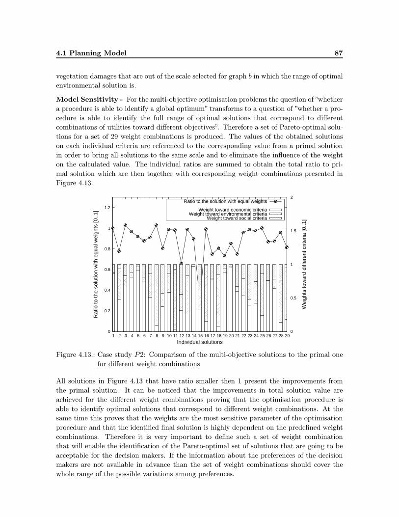
4.1 Planning Model 87
vegetation damages that are out of the scale selected for graph b in which the range of optimal
environmental solution is.
Model Sensitivity - For the multi-objective optimisation problems the question of ”whether
a procedure is able to identify a global optimum” transforms to a question of ”whether a pro-
cedure is able to identify the full range of optimal solutions that correspond to different
combinations of utilities toward different objectives”. Therefore a set of Pareto-optimal solu-
tions for a set of 29 weight combinations is produced. The values of the obtained solutions
on each individual criteria are referenced to the corresponding value from a primal solution
in order to bring all solutions to the same scale and to eliminate the influence of the weight
on the calculated value. The individual ratios are summed to obtain the total ratio to pri-
mal solution which are then together with corresponding weight combinations presented in
Figure 4.13.
0
0.2
0.4
0.6
0.8
1
1.2
1 2 3 4 5 6 7 8 9 10 11 12 13 14 15 16 17 18 19 20 21 22 23 24 25 26 27 28 29 0
0.5
1
1.5
2
Rat
io to
the
solu
tion
with
equ
al w
eigh
ts [0
..1]
Wei
ghts
tow
ard
diffe
rent
crit
eria
[0..1
]
Individual solutions
Ratio to the solution with equal weights
Weight toward economic criteriaWeight toward environmental criteria
Weight toward social criteria
Figure 4.13.: Case study P2: Comparison of the multi-objective solutions to the primal one
for different weight combinations
All solutions in Figure 4.13 that have ratio smaller then 1 present the improvements from
the primal solution. It can be noticed that the improvements in total solution value are
achieved for the different weight combinations proving that the optimisation procedure is
able to identify optimal solutions that correspond to different weight combinations. At the
same time this proves that the weights are the most sensitive parameter of the optimisation
procedure and that the identified final solution is highly dependent on the predefined weight
combinations. Therefore it is very important to define such a set of weight combination
that will enable the identification of the Pareto-optimal set of solutions that are going to be
acceptable for the decision makers. If the information about the preferences of the decision
makers are not available in advance than the set of weight combinations should cover the
whole range of the possible variations among preferences.
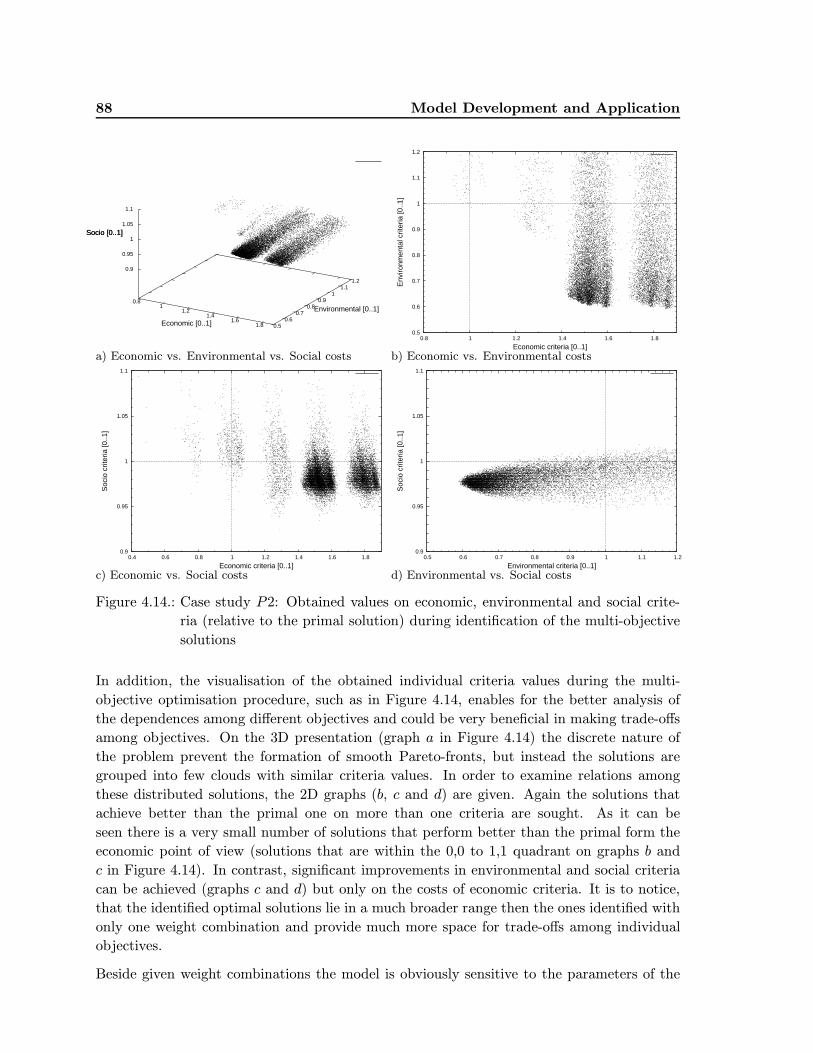
88 Model Development and Application
0.8 1
1.2 1.4
1.6 1.8 0.5
0.6 0.7
0.8 0.9
1 1.1
1.2
0.9
0.95
1
1.05
1.1
Socio [0..1]
Economic [0..1]
Environmental [0..1]
Socio [0..1]
a) Economic vs. Environmental vs. Social costs
0.5
0.6
0.7
0.8
0.9
1
1.1
1.2
0.8 1 1.2 1.4 1.6 1.8
Env
ironm
enta
l crit
eria
[0..1
]
Economic criteria [0..1]b) Economic vs. Environmental costs
0.9
0.95
1
1.05
1.1
0.4 0.6 0.8 1 1.2 1.4 1.6 1.8
Soc
io c
riter
ia [0
..1]
Economic criteria [0..1]c) Economic vs. Social costs
0.9
0.95
1
1.05
1.1
0.5 0.6 0.7 0.8 0.9 1 1.1 1.2
Soc
io c
riter
ia [0
..1]
Environmental criteria [0..1]d) Environmental vs. Social costs
Figure 4.14.: Case study P2: Obtained values on economic, environmental and social crite-
ria (relative to the primal solution) during identification of the multi-objective
solutions
In addition, the visualisation of the obtained individual criteria values during the multi-
objective optimisation procedure, such as in Figure 4.14, enables for the better analysis of
the dependences among different objectives and could be very beneficial in making trade-offs
among objectives. On the 3D presentation (graph a in Figure 4.14) the discrete nature of
the problem prevent the formation of smooth Pareto-fronts, but instead the solutions are
grouped into few clouds with similar criteria values. In order to examine relations among
these distributed solutions, the 2D graphs (b, c and d) are given. Again the solutions that
achieve better than the primal one on more than one criteria are sought. As it can be
seen there is a very small number of solutions that perform better than the primal form the
economic point of view (solutions that are within the 0,0 to 1,1 quadrant on graphs b and
c in Figure 4.14). In contrast, significant improvements in environmental and social criteria
can be achieved (graphs c and d) but only on the costs of economic criteria. It is to notice,
that the identified optimal solutions lie in a much broader range then the ones identified with
only one weight combination and provide much more space for trade-offs among individual
objectives.
Beside given weight combinations the model is obviously sensitive to the parameters of the
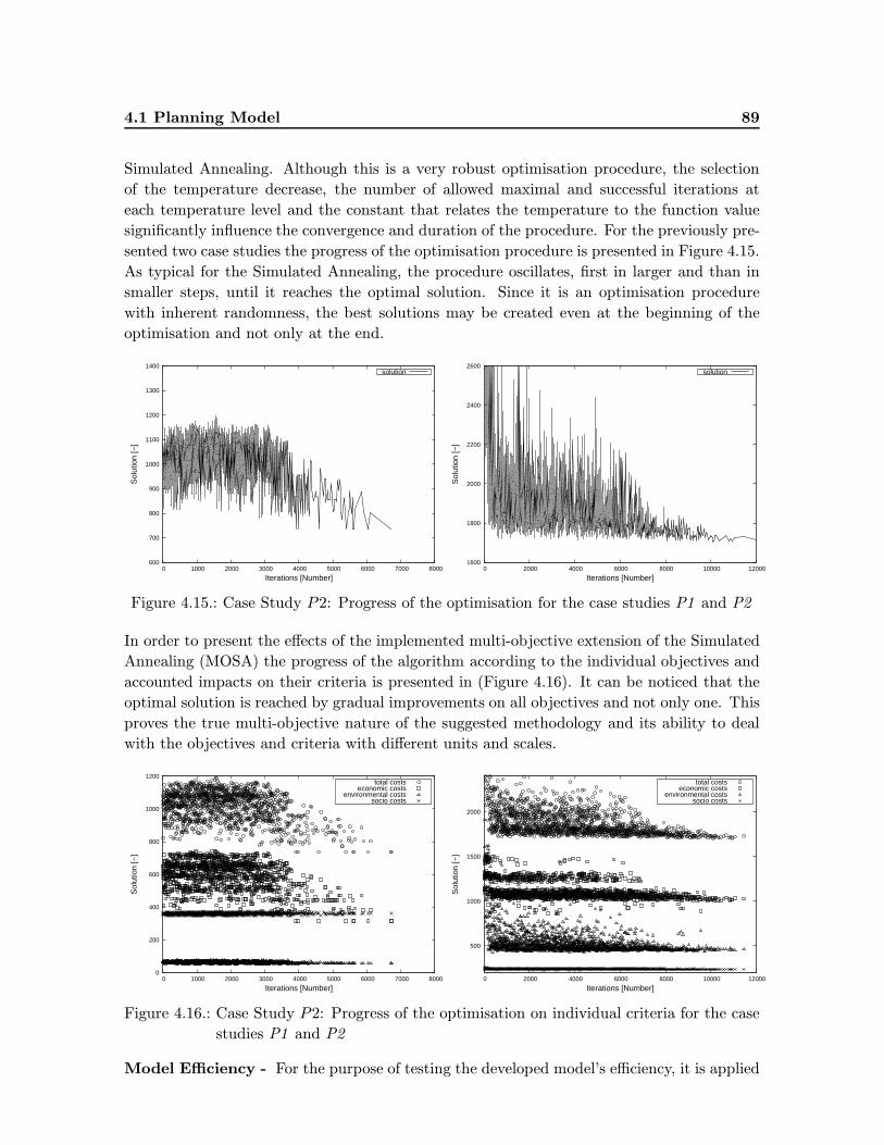
4.1 Planning Model 89
Simulated Annealing. Although this is a very robust optimisation procedure, the selection
of the temperature decrease, the number of allowed maximal and successful iterations at
each temperature level and the constant that relates the temperature to the function value
significantly influence the convergence and duration of the procedure. For the previously pre-
sented two case studies the progress of the optimisation procedure is presented in Figure 4.15.
As typical for the Simulated Annealing, the procedure oscillates, first in larger and than in
smaller steps, until it reaches the optimal solution. Since it is an optimisation procedure
with inherent randomness, the best solutions may be created even at the beginning of the
optimisation and not only at the end.
600
700
800
900
1000
1100
1200
1300
1400
0 1000 2000 3000 4000 5000 6000 7000 8000
Sol
utio
n [−
]
Iterations [Number]
solution
1600
1800
2000
2200
2400
2600
0 2000 4000 6000 8000 10000 12000
Sol
utio
n [−
]
Iterations [Number]
solution
Figure 4.15.: Case Study P2: Progress of the optimisation for the case studies P1 and P2
In order to present the effects of the implemented multi-objective extension of the Simulated
Annealing (MOSA) the progress of the algorithm according to the individual objectives and
accounted impacts on their criteria is presented in (Figure 4.16). It can be noticed that the
optimal solution is reached by gradual improvements on all objectives and not only one. This
proves the true multi-objective nature of the suggested methodology and its ability to deal
with the objectives and criteria with different units and scales.
0
200
400
600
800
1000
1200
0 1000 2000 3000 4000 5000 6000 7000 8000
Sol
utio
n [−
]
Iterations [Number]
total costseconomic costs
environmental costssocio costs
500
1000
1500
2000
0 2000 4000 6000 8000 10000 12000
Sol
utio
n [−
]
Iterations [Number]
total costseconomic costs
environmental costssocio costs
Figure 4.16.: Case Study P2: Progress of the optimisation on individual criteria for the case
studies P1 and P2
Model Efficiency - For the purpose of testing the developed model’s efficiency, it is applied
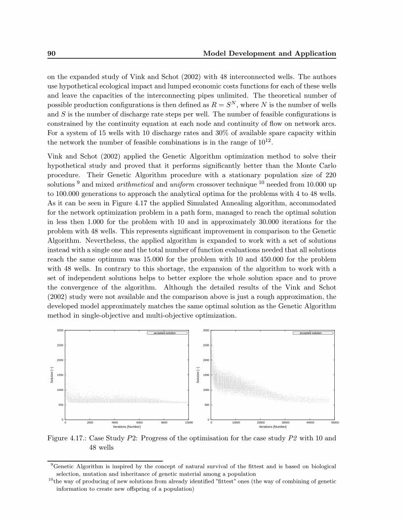
90 Model Development and Application
on the expanded study of Vink and Schot (2002) with 48 interconnected wells. The authors
use hypothetical ecological impact and lumped economic costs functions for each of these wells
and leave the capacities of the interconnecting pipes unlimited. The theoretical number of
possible production configurations is then defined as R = SN , where N is the number of wells
and S is the number of discharge rate steps per well. The number of feasible configurations is
constrained by the continuity equation at each node and continuity of flow on network arcs.
For a system of 15 wells with 10 discharge rates and 30% of available spare capacity within
the network the number of feasible combinations is in the range of 1012.
Vink and Schot (2002) applied the Genetic Algorithm optimization method to solve their
hypothetical study and proved that it performs significantly better than the Monte Carlo
procedure. Their Genetic Algorithm procedure with a stationary population size of 220
solutions 9 and mixed arithmetical and uniform crossover technique 10 needed from 10.000 up
to 100.000 generations to approach the analytical optima for the problems with 4 to 48 wells.
As it can be seen in Figure 4.17 the applied Simulated Annealing algorithm, accommodated
for the network optimization problem in a path form, managed to reach the optimal solution
in less then 1.000 for the problem with 10 and in approximately 30.000 iterations for the
problem with 48 wells. This represents significant improvement in comparison to the Genetic
Algorithm. Nevertheless, the applied algorithm is expanded to work with a set of solutions
instead with a single one and the total number of function evaluations needed that all solutions
reach the same optimum was 15.000 for the problem with 10 and 450.000 for the problem
with 48 wells. In contrary to this shortage, the expansion of the algorithm to work with a
set of independent solutions helps to better explore the whole solution space and to prove
the convergence of the algorithm. Although the detailed results of the Vink and Schot
(2002) study were not available and the comparison above is just a rough approximation, the
developed model approximately matches the same optimal solution as the Genetic Algorithm
method in single-objective and multi-objective optimization.
0
500
1000
1500
2000
2500
3000
0 2000 4000 6000 8000 10000
Sol
utio
n [−
]
Iterations [Number]
accepted solution
0
500
1000
1500
2000
2500
3000
0 10000 20000 30000 40000 50000
Sol
utio
n [−
]
Iterations [Number]
accepted solution
Figure 4.17.: Case Study P2: Progress of the optimisation for the case study P2 with 10 and
48 wells
9Genetic Algorithm is inspired by the concept of natural survival of the fittest and is based on biological
selection, mutation and inheritance of genetic material among a population10the way of producing of new solutions from already identified ”fittest” ones (the way of combining of genetic
information to create new offspring of a population)

4.2 Design Model 91
4.2. Design Model
Most of the existing water supply systems have been designed and built in the late 19th
and the 20th century. As any other man made systems, they are a reflection of the needs,
preferences, knowledge level and technical capabilities of the time when they were build up.
Although most of these systems are still well functioning, in recent decades, the interests
and expectations of water supply decision makers, managers and operators have changed.
The importance of better maintenance and operation, public and stakeholder participation,
management of water demands and environmental impacts and flexible and reliable systems
design and operation are just some of the new driving factors. Instead on focusing only on
technical and economic issues, the water supply designers are today increasingly interested
in the incorporation of the uncertainty aspects as well as in the risk and reliability issues. A
model that supports the development of multi-objective design alternatives, provides for the
system uncertainty and reliability quantification as well as risk-oriented system evaluation is
presented next.
4.2.1. Characterisation of the Design Problem
In general terms it can be stated that the main purpose of the water supply design is to
determine sizes and capacities for some, or all, system components in such a way to provide
for the proper functioning of a system under all design conditions for a whole design period
(Walski et al., 2003). Since the design conditions are often seen as all stresses which a system
is supposed to sustain during its life time, the design of water supply systems components is
often achieved by consecutive testing and improving of the system performance for some pre-
selected system stresses. Design conditions and design period as well as the main objectives of
the design depend on the individual project aims and characteristics, and can differ largely for
different systems (e.g. development of a new system or rehabilitation of an already existing
one) and the type of a design study (e.g. preliminary design or design of an individual system
component). Therefore the main objectives, the level of complexity and expectations from an
analysis may also differ greatly. Nevertheless, the most often found objectives in the design
of water supply systems can be categorized into:
1. Performance satisfaction, usually in terms of delivered flows and pressures.
2. Costs minimization, usually in terms of investment and operation costs.
3. Benefit maximization, often in terms of reliability of a system.
The first objective is usually considered as a necessary prerequisite for the successful operation
of water supply systems and is therefore mainly incorporated as constraint in the design
problem formulation, where the performance indicators, such as delivered flows and pressures
at demand nodes, have to achieve already established engineering standards such as minimum
and maximum node pressures, minimum fire-fighting flows, maximum pipe flow velocities,
etc. Although water supply systems are mainly not ”market-driven” and many social and
institutional factors may predominantly influence their real costs (e.g. subsidies, interests on
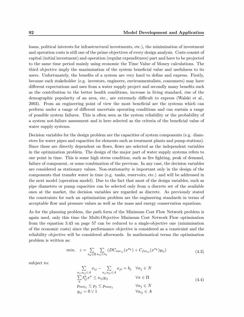
92 Model Development and Application
loans, political interests for infrastructural investments, etc.), the minimization of investment
and operation costs is still one of the prime objectives of every design analysis. Costs consist of
capital (initial investment) and operation (regular expenditures) part and have to be projected
to the same time period mainly using economic the Time Value of Money calculations. The
third objective imply the maximisation of the system beneficial value and usefulness to its
users. Unfortunately, the benefits of a system are very hard to define and express. Firstly,
because each stakeholder (e.g. investors, engineers, environmentalists, consumers) may have
different expectations and uses from a water supply project and secondly many benefits such
as the contribution to the better health conditions, increase in living standard, rise of the
demographic popularity of an area, etc., are extremely difficult to express (Walski et al.,
2003). From an engineering point of view the most beneficial are the systems which can
perform under a range of different uncertain operating conditions and can sustain a range
of possible system failures. This is often seen as the system reliability or the probability of
a system not-failure assessment and is here selected as the criteria of the beneficial value of
water supply systems.
Decision variables for the design problem are the capacities of system components (e.g. diam-
eters for water pipes and capacities for elements such as treatment plants and pump stations).
Since these are directly dependent on flows, flows are selected as the independent variables
in the optimization problem. The design of the major part of water supply systems refers to
one point in time. This is some high stress condition, such as fire fighting, peak of demand,
failure of component, or some combination of the previous. In any case, the decision variables
are considered as stationary values. Non-stationarity is important only in the design of the
components that transfer water in time (e.g. tanks, reservoirs, etc.) and will be addressed in
the next model (operation model). Due to the fact that most of the design variables, such as
pipe diameters or pump capacities can be selected only from a discrete set of the available
ones at the market, the decision variables are regarded as discrete. As previously stated
the constraints for such an optimization problem are the engineering standards in terms of
acceptable flow and pressure values as well as the mass and energy conservation equations.
As for the planning problem, the path form of the Minimum Cost Flow Network problem is
again used, only this time the Multi-Objective Minimum Cost Network Flow optimisation
from the equation 3.43 on page 57 can be reduced to a single-objective one (minimisation
of the economic costs) since the performance objective is considered as a constraint and the
reliability objective will be considered afterwards. In mathematical terms the optimisation
problem is written as:
min. z =∑
πk∈Π
∑
aij∈πk
(DCvarij (xπk) + Cfixij
(xπk)yij) (4.3)
subject to: ∑
nj :aij∈Axij −
∑
nj :aji∈Axji = bj ∀nj ∈ N
∑
πδπijx
π ≤ κijyij ∀π ∈ Π
pminj ≤ pj ≤ pmaxj ∀nj ∈ N
yij = 0 ∨ 1 ∀aij ∈ A
(4.4)
4.2 Design Model 93
where xπ is a path flow on a conforming simple path π 11 and the collection of x = {xπk | πk ∈Π} of all conforming paths Π is a network flow vector. Individual arc flows can be obtained
as xij =∑
πδπijx
π for δπij = 1 if an arc aij is on the path xπ and 0 otherwise. Unit-functions
C are scaled representatives of the net-cost (impact) functions c that depict the impacts of
some system parameter such as flow in this case. Furthermore, the variable costs Cvar are
discounted to their net present value DCvar in order to bring them to the same time scale
as the fixed costs Cfix. Already existing system elements have only variable costs (yij = 0),
while the potential elements (new or elements under rehabilitation) may have a fixed part
(yij = 1), too. Parameter κij stands for the upper capacity limit of an arc aij while pminj
and pmaxj stand for the minimum and maximum standard pressure values at a node nj,
respectively.
Although in the design problem a single-objective mathematical formulation of the optimi-
sation problem is used (minimisation of economic costs), the multi-objective nature of the
design is encompassed by introducing the performance satisfaction objective as a constraint
in the mathematical formulation and by introducing an additional step for dealing with the
third objective (reliability maximization or maximization of the probability of not failure).
This is necessary, since the probability of a system not failure can be calculated only for an
already defined system configuration and represents an additional way to handle complex
multi objective problems (decomposition approach). The design problem is separated into:
1) the identification of minimum cost system configurations that satisfy needed performances
(primal solution) and 2) evaluation of the reliability of these configurations and for different
levels of decision makers’ risk-tolerance (final solution. The selection of the optimal design
solution is than a trade-off among system costs and system reliability.
PRIMAL SOLUTION
(minimum cost system configuration)
FINAL SOLUTIONS
(reliable system configuration)
DECOMPOSITIONsolution that has minimum economic costs and satisfy predefined performance criteria
solutions that sustain predefined component failure scenarios and satisfy certain level of performance failures for uncertain input parameters
PERFORMANCE CALCULATION
Figure 4.18.: Decomposition applied in the design model
11directed path from a source node ns to a destination node nd
94 Model Development and Application
4.2.2. Accommodation of the Solution Methodology
The solution technique for the defined design optimization problem should be capable of
efficiently dealing with the following main tasks:
1. Representation of the water supply system structure and function.
2. Creation of minimum cost design alternative configurations.
3. Reliability assessment based on failure analysis and parameters’ uncertainty.
The selected network representation is not just convenient for the water supply systems struc-
ture and function representation, but it also has a capability to include layout considerations
in the design analysis. As proved by Goulter (1987) the layout of a system significantly influ-
ences not just its investment and operation costs but it also affects the reliability of a system.
In addition, network representation may be used to improve, or constraint, the optimization
algorithms, since it provide for the effective subdivision of the problem into sub-problems on
sub-networks. The adopted design model concept based on the directed network represen-
tation of water supply systems, is very similar to the Diba et al. (1995) methodology, only
the directed graph algorithms are not used just for the pre and post-processing of the opti-
mization algorithm, but they are internally integrated in the optimization procedure. This
decreases the computational demand during the exchange of parameters and enable efficient
iterative running of the optimisation procedure. Furthermore, the general procedure for the
identification of the minimum cost network flows from Jensen (1980) is combined with the
connectivity analysis12 of Ostfeld and Shamir (1996); Ostfeld (2005), in order to promote the
exploration of the entire network topology when developing alternative design options. In
addition, the first algorithm is accommodated to deal with the minimum cost flow problem
defined in the path form and the consideration of the pressure constraint is added to the
second algorithm. Although many optimization models work as well without any particular
system representation, it may be stated, that exactly the possibility to clearly represent water
supply systems structure and function within the optimisation model may be the prevailing
factor in increasing the acceptance and applicability of the optimisation methods.
Since the water supply distribution network design problem itself (selection of the sizes for
N elements from a predefined set of M sizes) has an exponential time complexity function
O(MN ) and very complex functional relations among criteria and system parameters (e.g.
flow and pressure distribution depend on the whole network configuration), large water sup-
ply systems are often too complex to be solved by exact (analytical) optimization methods
(Walski et al., 2003). The methods that create a possible solution, or a set of solutions,
check the function value against already obtained solutions and iteratively progress toward
more optimal solutions are often referred as approximate methods and present a good alter-
native for exact methods. Although they do not guarantee the identification of the global
optimum and declare only the best found solution, they are often able to identify not just
one but a set of very good (near optimal) solutions. The optimization procedure suggested
12a water supply systems layout analysis based on the examination of the paths between all individual source
and demand nodes
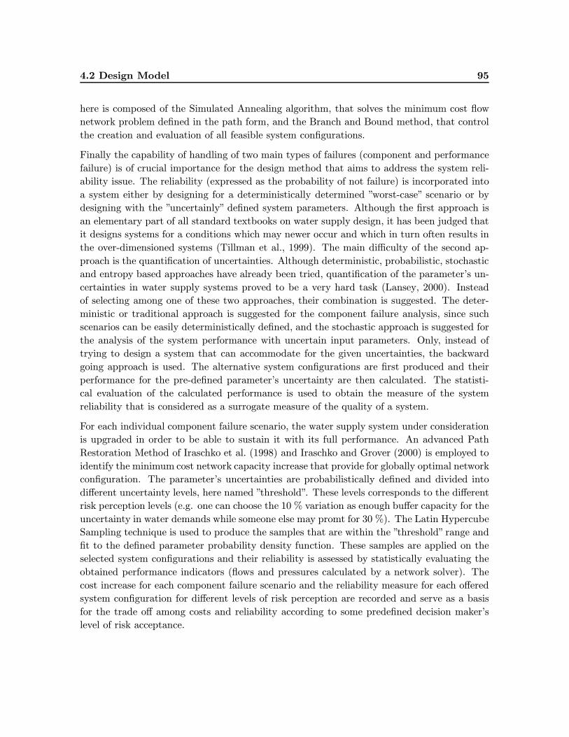
4.2 Design Model 95
here is composed of the Simulated Annealing algorithm, that solves the minimum cost flow
network problem defined in the path form, and the Branch and Bound method, that control
the creation and evaluation of all feasible system configurations.
Finally the capability of handling of two main types of failures (component and performance
failure) is of crucial importance for the design method that aims to address the system reli-
ability issue. The reliability (expressed as the probability of not failure) is incorporated into
a system either by designing for a deterministically determined ”worst-case” scenario or by
designing with the ”uncertainly” defined system parameters. Although the first approach is
an elementary part of all standard textbooks on water supply design, it has been judged that
it designs systems for a conditions which may newer occur and which in turn often results in
the over-dimensioned systems (Tillman et al., 1999). The main difficulty of the second ap-
proach is the quantification of uncertainties. Although deterministic, probabilistic, stochastic
and entropy based approaches have already been tried, quantification of the parameter’s un-
certainties in water supply systems proved to be a very hard task (Lansey, 2000). Instead
of selecting among one of these two approaches, their combination is suggested. The deter-
ministic or traditional approach is suggested for the component failure analysis, since such
scenarios can be easily deterministically defined, and the stochastic approach is suggested for
the analysis of the system performance with uncertain input parameters. Only, instead of
trying to design a system that can accommodate for the given uncertainties, the backward
going approach is used. The alternative system configurations are first produced and their
performance for the pre-defined parameter’s uncertainty are then calculated. The statisti-
cal evaluation of the calculated performance is used to obtain the measure of the system
reliability that is considered as a surrogate measure of the quality of a system.
For each individual component failure scenario, the water supply system under consideration
is upgraded in order to be able to sustain it with its full performance. An advanced Path
Restoration Method of Iraschko et al. (1998) and Iraschko and Grover (2000) is employed to
identify the minimum cost network capacity increase that provide for globally optimal network
configuration. The parameter’s uncertainties are probabilistically defined and divided into
different uncertainty levels, here named ”threshold”. These levels corresponds to the different
risk perception levels (e.g. one can choose the 10 % variation as enough buffer capacity for the
uncertainty in water demands while someone else may promt for 30 %). The Latin Hypercube
Sampling technique is used to produce the samples that are within the ”threshold” range and
fit to the defined parameter probability density function. These samples are applied on the
selected system configurations and their reliability is assessed by statistically evaluating the
obtained performance indicators (flows and pressures calculated by a network solver). The
cost increase for each component failure scenario and the reliability measure for each offered
system configuration for different levels of risk perception are recorded and serve as a basis
for the trade off among costs and reliability according to some predefined decision maker’s
level of risk acceptance.
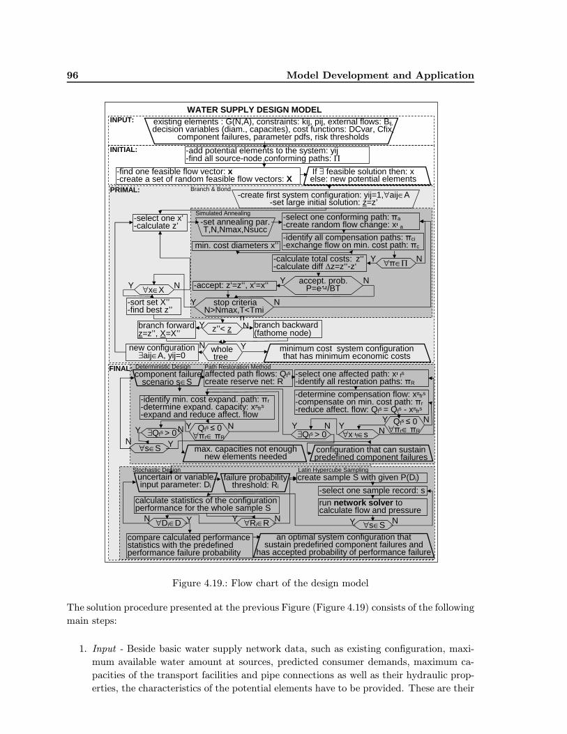
96 Model Development and Application
WATER SUPPLY DESIGN MODELexisting elements : G(N,A), constraints: kij, pij, external flows: Bij, decision variables (diam., capacites), cost functions: DCvar, Cfix,
component failures, parameter pdfs, risk thresholds
-find one feasible flow vector: x-create a set of random feasible flow vectors: X
INPUT:
-add potential elements to the system: yij-find all source-node conforming paths: Π
-select one affected path: xπfs
-identify all restoration paths: πR
-determine compensation flow: xπfrs
-compensate on min. cost path: πr-reduce affect. flow: Qfs = Qfs - xπfrs
Y∀xπf∈s N
affected path flows: Qfs
create reserve net: Rcomponent failure
scenario s∈S
INITIAL:
Y
-create first system configuration: yij=1,∀aij∈A-set large initial solution: z=z’
-select one conforming path: πa-create random flow change: xπa
-identify all compensation paths: πci-exchange flow on min. cost path: πc
accept. prob.P=e∆z/BT
-set annealing par.T,N,Nmax,Nsucc
-calculate total costs: z‘‘-calculate diff ∆z=z‘‘-z‘
N
Y ∀π∈Π N
-accept: z‘=z‘‘, x‘=x‘‘
Y stop criteriaN>Nmax,T<Tmi
n
N
Y z’’< z N
-select one x’-calculate z’
Y ∀x∈X N
-sort set X’’-find best z’’
branch forwardz=z’’, X=X’’
branch backward(fathome node)
N wholetree
Ynew configuration∃aij∈A, yij=0
minimum cost system configuration that has minimum economic costs
PRIMAL: Branch & Bond
Simulated Annealing
If ∃ feasible solution then: xelse: new potential elements
FINAL: Deterministic Design
min. cost diameters x’’
Y Qfs ≤ 0∀πr∈ πR
NY
∃Qfs > 0N
-identify min. cost expand. path: πr-determine expand. capacity: xπfrs
-expand and reduce affect. flow
Qfs ≤ 0∀πr∈ πR
NYY ∃Qfs > 0N
max. capacities not enoughnew elements needed
configuration that can sustainpredefined component failures
uncertain or variableinput parameter: Di
Latin Hypercube Sampling
N Y∀s∈S
create sample S with given P(Di)
-select one sample record: s
run network solver tocalculate flow and pressure
Y N∀s∈S
calculate statistics of the configurationperformance for the whole sample S
compare calculated performance statistics with the predefinedperformance failure probability
failure probabilitythreshold: Ri
Y N∀Ri∈RN Y∀Di∈D
an optimal system configuration thatsustain predefined component failures and
has accepted probability of performance failure
Stochastic Design
Path Restoration Method
Figure 4.19.: Flow chart of the design model
The solution procedure presented at the previous Figure (Figure 4.19) consists of the following
main steps:
1. Input - Beside basic water supply network data, such as existing configuration, maxi-
mum available water amount at sources, predicted consumer demands, maximum ca-
pacities of the transport facilities and pipe connections as well as their hydraulic prop-
erties, the characteristics of the potential elements have to be provided. These are their
4.2 Design Model 97
potential position and set of discrete values of their possible capacities together with
investment and operation costs functions. In addition, the component failure scenarios,
the probability density function of the uncertain parameters and the acceptable risk
”threshold” values for the reliability evaluation have to be defined.
2. Initial solution - feasible solution without costs - A graph procedure based on the al-
location of maximum flows on paths between source and demand nodes is employed
to identify one flow vector that satisfy all demands and does not violate capacity con-
straints. Cost functions are not considered for this solution.
3. Primal solutions - minimization of costs - The Branch and Bound algorithm is used
to explore all possible system configurations (addition of potential elements) while the
Simulated Annealing algorithm is employed to identify the minimum cost network flow
for which the minimum cost pipe diameters are determined. Different system config-
urations are compared until all branches of the Branch and Bound tree are explored.
The primal solution essentially represents the minimum cost water supply system con-
figuration in terms of its layout and component’s capacities.
4. Final solutions - maximization of reliability - In order to increase the reliability of the
identified configuration, the predefined component failure scenarios are incrementally
ran. For each scenario, minimum cost spare capacities are added to the system in a
way to provide its function without the failed component. The degradations of the
minimum cost objective for each failure scenario are recorded. Additionally for each
risk-acceptance ”threshold” value, the system reliability is assessed by statistically eval-
uating the network flows and pressures calculated with network solver of Gessler et al.
(1985), for the samples of uncertain parameters (e.g. water demands) created with an
advance sampling method of Iman and Shortencarier (1984). Since the ”threshold” va-
lues correspond to the uncertainty levels that one has to accept as the range of possible
deviations of the uncertain parameters, they define the acceptable risk level that the
decision makers are ready to accept in selection of the solution. The risk acceptable
level, system cost and its reliability represent the main criteria for the selection of the
final design solution.
4.2.3. Case Study D1 - Design Model Demonstration
Study Description - In order to present the purpose and illustrate some capabilities of the
developed design model, the same case study as for the planning model is used. This is an
adaptation of the study of Alperovits and Shamir (1977) that considers the design of a water
distribution network with 4 water sources (river, groundwater and two spring water sources),
6 consumer nodes (out of which 2 are new) and 11 arcs that connect these elements. In
addition to the network description and characteristics given in subchapter 4.1.3 on page 72,
the set of commercially available water pipes and their costs per unit meter of length had to
be defined. The set of 14 pipe diameters, that is mainly used in water supply optimisation
literature, where pipe diameters are given in inches (1 inch = 25.4 mm) and pipe investment
costs (fixed costs) are given in dollars per meter of length, is selected as the set of the possible

98 Model Development and Application
decision variables. It originate from the same study of Alperovits and Shamir (1977) and is
presented in Table 4.4. It is to be noticed that the operation costs (variable costs) are not
included in the standard formulation of the water supply design problem and will be addressed
in the next management stage, namely in the operation stage.
D [inch] 1 2 3 4 6 8 10 12 14 16 18 20 22 24D [mm] 25.4 50.8 76.2 101.6 152.4 203.2 254.0 304.8 355.6 406.4 457.2 508.7 558.8 609.6C [$/m] 2 5 8 11 16 23 32 50 60 90 130 170 300 550
Table 4.4.: Case Study D1: Standard set of available pipe diameters with their investment
costs per unit length [source: Alperovits and Shamir (1977)]
Problem Statement - The design analysis is logical extension of the planning analysis in
which for some identified network general configuration the capacities of network elements
are to be determined. Therefore one of the Pareto-optimal planning solutions, presented in
the previous chapter (Environmentally optimal) is used as an input network configuration
for the design analysis. The selected solution is the one that favours the use of all three new
water sources (N8, N9, and N10 ) and suggests building of the new transport arcs A8, A9,
A10, A11. In addition to these new elements, the rehabilitation of the existing arcs A4 and
A6 is also included in the consideration. The network configuration and the characteristics
of the selected planning solution are given in Figure 4.20.
arc capacity [m3/hr]K
pipe (arc) to rehabilitate
potential pipe (arc)
existing pipe (arc)
demand point (node)
transport point (node)
source point (node)
N: 3
node external flow [m3/hr]B
arc flow [m3/hr]F
arc length [m]L
Figure 4.20.: Case study D1: Network configuration of the selected planning solution
The stated objectives of the performance satisfaction, costs minimisation and benefits max-
imisation are obviously conflicting. The smallest possible elements sizes that provide for the
satisfactory flows and pressures, within some water supply network yield the minimum in-
vestment costs. The reliable functioning of a water supply system under different operating
conditions, uncertain parameter values and emergency or failure situations, demands for the
existence of some spare capacities, whose addition obviously ruin the minimum investment
cost criterion. The compromise among these two objectives is the predominate question in
the design of water supply systems. Due to the fact that the reliability assessment can be
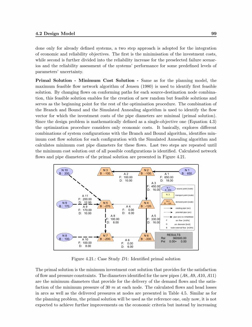
4.2 Design Model 99
done only for already defined systems, a two step approach is adopted for the integration
of economic and reliability objectives. The first is the minimisation of the investment costs,
while second is further divided into the reliability increase for the preselected failure scenar-
ios and the reliability assessment of the systems’ performance for some predefined levels of
parameters’ uncertainty.
Primal Solution - Minimum Cost Solution - Same as for the planning model, the
maximum feasible flow network algorithm of Jensen (1980) is used to identify first feasible
solution. By changing flows on conforming paths for each source-destination node combina-
tion, this feasible solution enables for the creation of new random but feasible solutions and
serves as the beginning point for the rest of the optimisation procedure. The combination of
the Branch and Bound and the Simulated Annealing algorithm is used to identify the flow
vector for which the investment costs of the pipe diameters are minimal (primal solution).
Since the design problem is mathematically defined as a single-objective one (Equation 4.3)
the optimization procedure considers only economic costs. It basically, explores different
combinations of system configurations with the Branch and Bound algorithm, identifies min-
imum cost flow solution for each configuration with the Simulated Annealing algorithm and
calculates minimum cost pipe diameters for these flows. Last two steps are repeated until
the minimum cost solution out of all possible configurations is identified. Calculated network
flows and pipe diameters of the primal solution are presented in Figure 4.21.
pipe (arc) to rehabilitate
potential pipe (arc)
existing pipe (arc)
demand point (node)
transport point (node)
source point (node)
N: 3
node external flow [m3/hr]B
arc flow [m3/hr]F
arc diameter [inch]D
Figure 4.21.: Case Study D1: Identified primal solution
The primal solution is the minimum investment cost solution that provides for the satisfaction
of flow and pressure constraints. The diameters identified for the new pipes (A8, A9, A10, A11)
are the minimum diameters that provide for the delivery of the demand flows and the satis-
faction of the minimum pressure of 30 m at each node. The calculated flows and head losses
in arcs as well as the delivered pressures at nodes are presented in Table 4.5. Similar as for
the planning problem, the primal solution will be used as the reference one, only now, it is not
expected to achieve further improvements on the economic criteria but instead by increasing
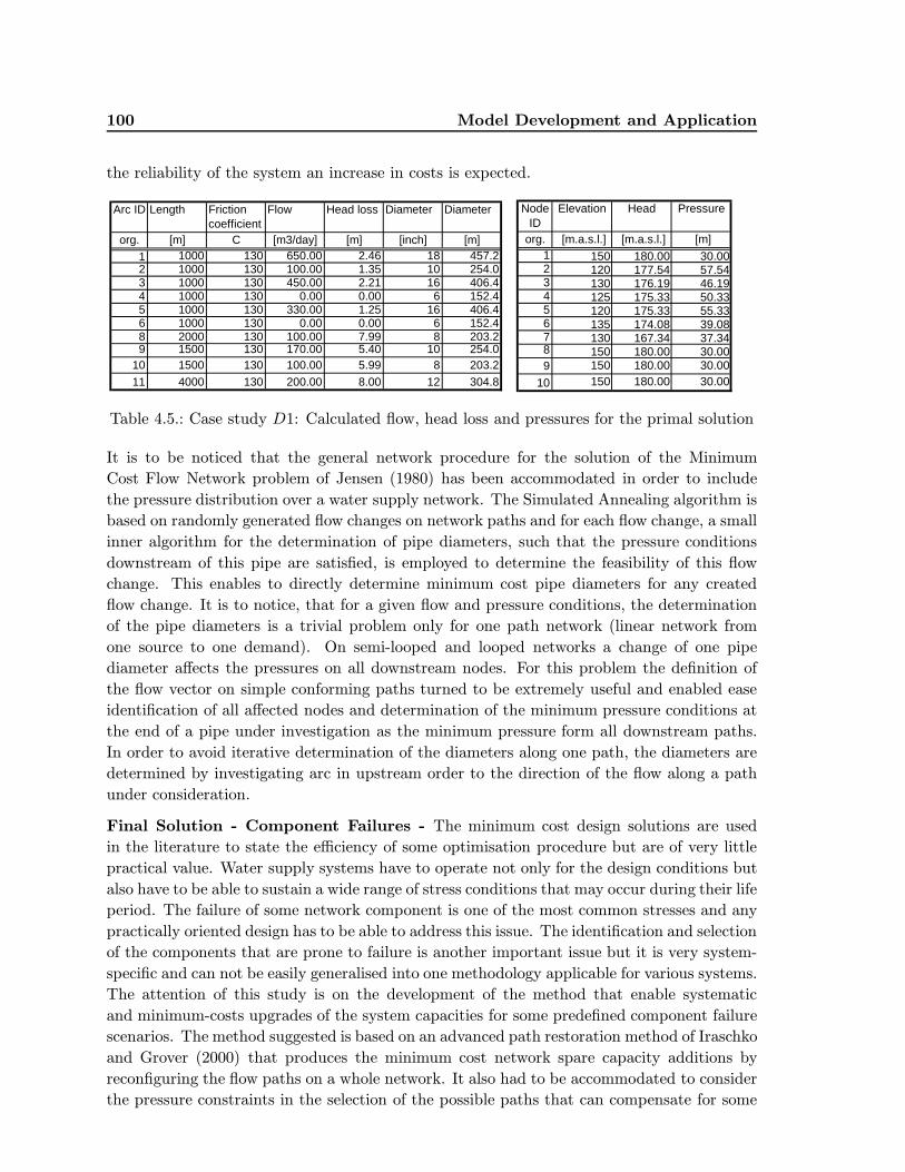
100 Model Development and Application
the reliability of the system an increase in costs is expected.
Arc ID Length Friction coefficient
Flow Head loss Diameter Diameter
org. [m] C [m3/day] [m] [inch] [m]
1 1000 130 650.00 2.46 18 457.22 1000 130 100.00 1.35 10 254.03 1000 130 450.00 2.21 16 406.44 1000 130 0.00 0.00 6 152.45 1000 130 330.00 1.25 16 406.46 1000 130 0.00 0.00 6 152.48 2000 130 100.00 7.99 8 203.29 1500 130 170.00 5.40 10 254.0
10 1500 130 100.00 5.99 8 203.2
11 4000 130 200.00 8.00 12 304.8
Node ID
Elevation Head Pressure
org. [m.a.s.l.] [m.a.s.l.] [m]1 150 180.00 30.002 120 177.54 57.543 130 176.19 46.194 125 175.33 50.335 120 175.33 55.336 135 174.08 39.087 130 167.34 37.348 150 180.00 30.009 150 180.00 30.00
10 150 180.00 30.00
Table 4.5.: Case study D1: Calculated flow, head loss and pressures for the primal solution
It is to be noticed that the general network procedure for the solution of the Minimum
Cost Flow Network problem of Jensen (1980) has been accommodated in order to include
the pressure distribution over a water supply network. The Simulated Annealing algorithm is
based on randomly generated flow changes on network paths and for each flow change, a small
inner algorithm for the determination of pipe diameters, such that the pressure conditions
downstream of this pipe are satisfied, is employed to determine the feasibility of this flow
change. This enables to directly determine minimum cost pipe diameters for any created
flow change. It is to notice, that for a given flow and pressure conditions, the determination
of the pipe diameters is a trivial problem only for one path network (linear network from
one source to one demand). On semi-looped and looped networks a change of one pipe
diameter affects the pressures on all downstream nodes. For this problem the definition of
the flow vector on simple conforming paths turned to be extremely useful and enabled ease
identification of all affected nodes and determination of the minimum pressure conditions at
the end of a pipe under investigation as the minimum pressure form all downstream paths.
In order to avoid iterative determination of the diameters along one path, the diameters are
determined by investigating arc in upstream order to the direction of the flow along a path
under consideration.
Final Solution - Component Failures - The minimum cost design solutions are used
in the literature to state the efficiency of some optimisation procedure but are of very little
practical value. Water supply systems have to operate not only for the design conditions but
also have to be able to sustain a wide range of stress conditions that may occur during their life
period. The failure of some network component is one of the most common stresses and any
practically oriented design has to be able to address this issue. The identification and selection
of the components that are prone to failure is another important issue but it is very system-
specific and can not be easily generalised into one methodology applicable for various systems.
The attention of this study is on the development of the method that enable systematic
and minimum-costs upgrades of the system capacities for some predefined component failure
scenarios. The method suggested is based on an advanced path restoration method of Iraschko
and Grover (2000) that produces the minimum cost network spare capacity additions by
reconfiguring the flow paths on a whole network. It also had to be accommodated to consider
the pressure constraints in the selection of the possible paths that can compensate for some
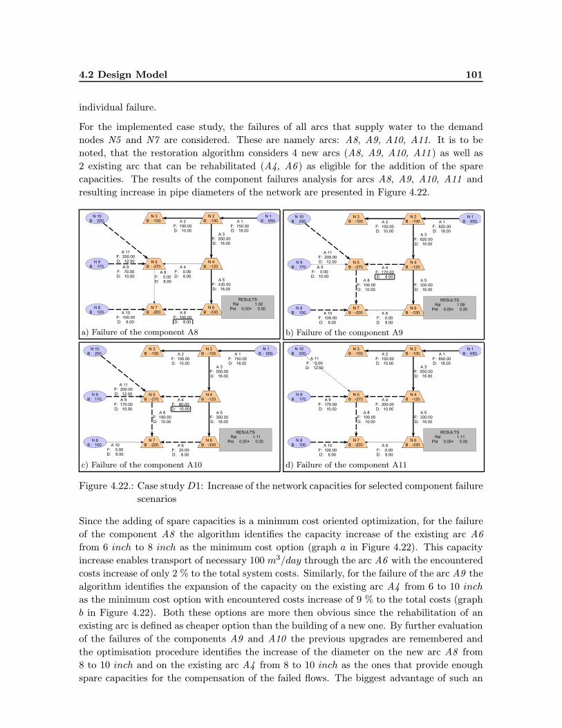
4.2 Design Model 101
individual failure.
For the implemented case study, the failures of all arcs that supply water to the demand
nodes N5 and N7 are considered. These are namely arcs: A8, A9, A10, A11. It is to be
noted, that the restoration algorithm considers 4 new arcs (A8, A9, A10, A11 ) as well as
2 existing arc that can be rehabilitated (A4, A6 ) as eligible for the addition of the spare
capacities. The results of the component failures analysis for arcs A8, A9, A10, A11 and
resulting increase in pipe diameters of the network are presented in Figure 4.22.
a) Failure of the component A8
b) Failure of the component A9
c) Failure of the component A10
d) Failure of the component A11
Figure 4.22.: Case studyD1: Increase of the network capacities for selected component failure
scenarios
Since the adding of spare capacities is a minimum cost oriented optimization, for the failure
of the component A8 the algorithm identifies the capacity increase of the existing arc A6
from 6 inch to 8 inch as the minimum cost option (graph a in Figure 4.22). This capacity
increase enables transport of necessary 100 m3/day through the arc A6 with the encountered
costs increase of only 2 % to the total system costs. Similarly, for the failure of the arc A9 the
algorithm identifies the expansion of the capacity on the existing arc A4 from 6 to 10 inch
as the minimum cost option with encountered costs increase of 9 % to the total costs (graph
b in Figure 4.22). Both these options are more then obvious since the rehabilitation of an
existing arc is defined as cheaper option than the building of a new one. By further evaluation
of the failures of the components A9 and A10 the previous upgrades are remembered and
the optimisation procedure identifies the increase of the diameter on the new arc A8 from
8 to 10 inch and on the existing arc A4 from 8 to 10 inch as the ones that provide enough
spare capacities for the compensation of the failed flows. The biggest advantage of such an
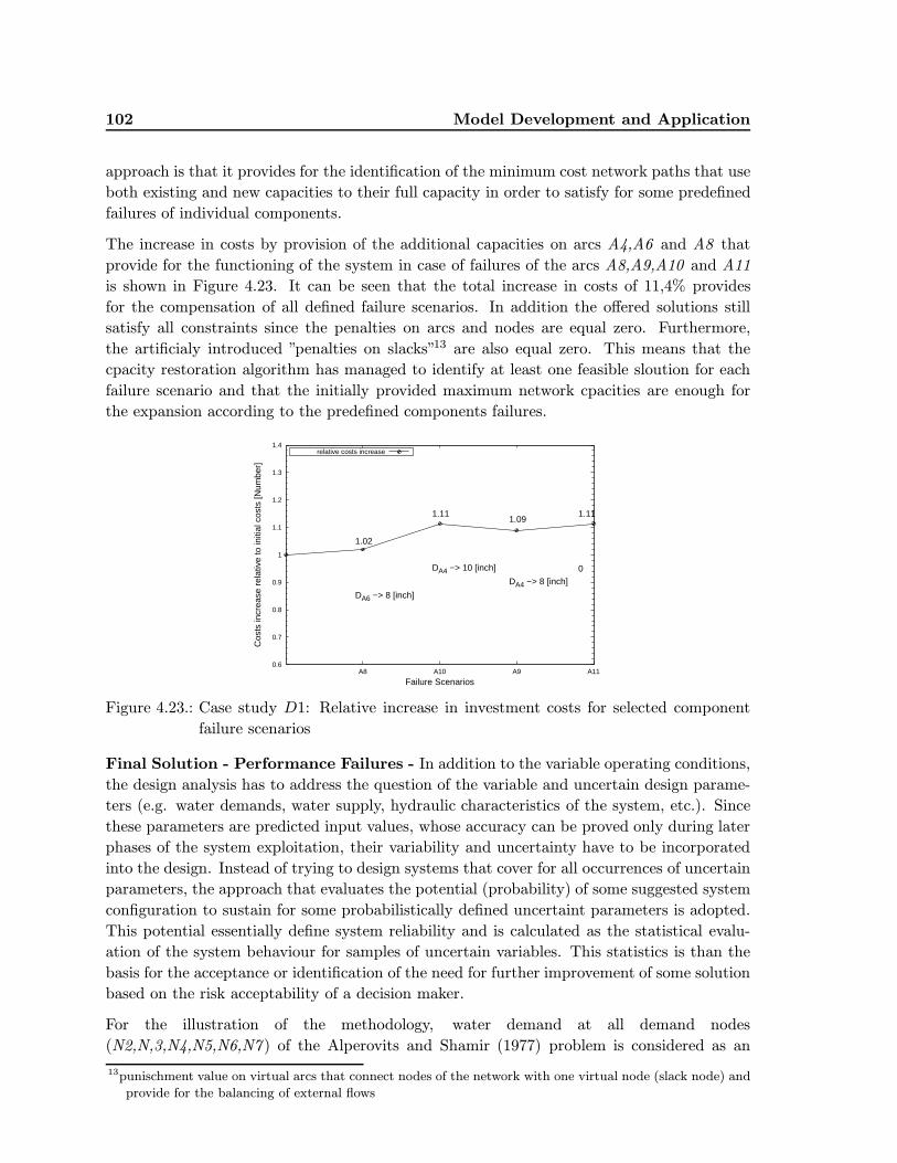
102 Model Development and Application
approach is that it provides for the identification of the minimum cost network paths that use
both existing and new capacities to their full capacity in order to satisfy for some predefined
failures of individual components.
The increase in costs by provision of the additional capacities on arcs A4,A6 and A8 that
provide for the functioning of the system in case of failures of the arcs A8,A9,A10 and A11
is shown in Figure 4.23. It can be seen that the total increase in costs of 11,4% provides
for the compensation of all defined failure scenarios. In addition the offered solutions still
satisfy all constraints since the penalties on arcs and nodes are equal zero. Furthermore,
the artificialy introduced ”penalties on slacks”13 are also equal zero. This means that the
cpacity restoration algorithm has managed to identify at least one feasible sloution for each
failure scenario and that the initially provided maximum network cpacities are enough for
the expansion according to the predefined components failures.
0.6
0.7
0.8
0.9
1
1.1
1.2
1.3
1.4
A8 A10 A9 A11
Cos
ts in
crea
se r
elat
ive
to in
itial
cos
ts [N
umbe
r]
Failure Scenarios
1.02
DA6 −> 8 [inch]
1.11
DA4 −> 10 [inch]
1.09
DA4 −> 8 [inch]
1.11
0
relative costs increase
Figure 4.23.: Case study D1: Relative increase in investment costs for selected component
failure scenarios
Final Solution - Performance Failures - In addition to the variable operating conditions,
the design analysis has to address the question of the variable and uncertain design parame-
ters (e.g. water demands, water supply, hydraulic characteristics of the system, etc.). Since
these parameters are predicted input values, whose accuracy can be proved only during later
phases of the system exploitation, their variability and uncertainty have to be incorporated
into the design. Instead of trying to design systems that cover for all occurrences of uncertain
parameters, the approach that evaluates the potential (probability) of some suggested system
configuration to sustain for some probabilistically defined uncertaint parameters is adopted.
This potential essentially define system reliability and is calculated as the statistical evalu-
ation of the system behaviour for samples of uncertain variables. This statistics is than the
basis for the acceptance or identification of the need for further improvement of some solution
based on the risk acceptability of a decision maker.
For the illustration of the methodology, water demand at all demand nodes
(N2,N,3,N4,N5,N6,N7 ) of the Alperovits and Shamir (1977) problem is considered as an
13punischment value on virtual arcs that connect nodes of the network with one virtual node (slack node) and
provide for the balancing of external flows
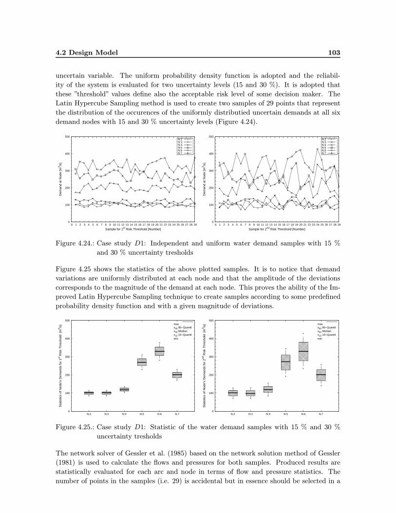
4.2 Design Model 103
uncertain variable. The uniform probability density function is adopted and the reliabil-
ity of the system is evaluated for two uncertainty levels (15 and 30 %). It is adopted that
these ”threshold” values define also the acceptable risk level of some decision maker. The
Latin Hypercube Sampling method is used to create two samples of 29 points that represent
the distribution of the occurences of the uniformly distributied uncertain demands at all six
demand nodes with 15 and 30 % uncertainty levels (Figure 4.24).
0
100
200
300
400
500
0 1 2 3 4 5 6 7 8 9 10 11 12 13 14 15 16 17 18 19 20 21 22 23 24 25 26 27 28 29
Dem
and
at N
ode
[m3 /s
]
Sample for 1st Risk Threshold [Number]
N:2N:3N:4N:5N:6N:7
0
100
200
300
400
500
0 1 2 3 4 5 6 7 8 9 10 11 12 13 14 15 16 17 18 19 20 21 22 23 24 25 26 27 28 29
Dem
and
at N
ode
[m3 /s
]
Sample for 2nd Risk Threshold [Number]
N:2N:3N:4N:5N:6N:7
Figure 4.24.: Case study D1: Independent and uniform water demand samples with 15 %
and 30 % uncertainty tresholds
Figure 4.25 shows the statistics of the above plotted samples. It is to notice that demand
variations are uniformly distributed at each node and that the amplitude of the deviations
corresponds to the magnitude of the demand at each node. This proves the ability of the Im-
proved Latin Hypercube Sampling technique to create samples according to some predefined
probability density function and with a given magnitude of deviations.
0
100
200
300
400
500
N:2 N:3 N:4 N:5 N:6 N:7
Sta
tistic
s of
Nod
e’s
Dem
ands
for
1st R
isk
Thr
esho
ld [
m3 /s
]
minx10 10−Quantilx50 Medianx90 90−Quantilmax
0
100
200
300
400
500
N:2 N:3 N:4 N:5 N:6 N:7
Sta
tistic
s of
Nod
e’s
Dem
ands
for
2nd R
isk
Thr
esho
ld [
m3 /s
]
minx10 10−Quantilx50 Medianx90 90−Quantilmax
Figure 4.25.: Case study D1: Statistic of the water demand samples with 15 % and 30 %
uncertainty tresholds
The network solver of Gessler et al. (1985) based on the network solution method of Gessler
(1981) is used to calculate the flows and pressures for both samples. Produced results are
statistically evaluated for each arc and node in terms of flow and pressure statistics. The
number of points in the samples (i.e. 29) is accidental but in essence should be selected in a
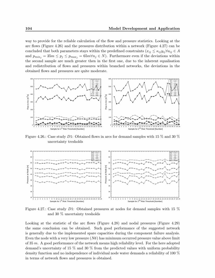
104 Model Development and Application
way to provide for the reliable calculation of the flow and pressure statistics. Looking at the
arc flows (Figure 4.26) and the pressures distribution within a network (Figure 4.27) can be
concluded that both parameters stays within the predefined constraints (xij ≤ κijyij∀aij ∈ A
and pminj = 35m ≤ pj ≤ pmaxj = 65m∀nj ∈ N). Furthermore even if the deviations within
the second sample are much greater then in the first one, due to the inherent equalisation
and redistribution of flows and pressures within branched networks, the deviations in the
obtained flows and pressures are quite moderate.
0
100
200
300
400
500
600
0 1 2 3 4 5 6 7 8 9 10 11 12 13 14 15 16 17 18 19 20 21 22 23 24 25 26 27 28 29
Flo
w in
Arc
[m3 /s
]
Sample for 1st Risk Threshold [Number]
A:1A:2A:3A:4A:5A:6A:7A:8A:9
A:10A:11
0
100
200
300
400
500
600
0 1 2 3 4 5 6 7 8 9 10 11 12 13 14 15 16 17 18 19 20 21 22 23 24 25 26 27 28 29
Flo
w in
Arc
[m3 /s
]
Sample for 2nd Risk Threshold [Number]
A:1A:2A:3A:4A:5A:6A:7A:8A:9
A:10A:11
Figure 4.26.: Case study D1: Obtained flows in arcs for demand samples with 15 % and 30 %
uncertainty tresholds
25
30
35
40
45
50
55
60
65
0 1 2 3 4 5 6 7 8 9 10 11 12 13 14 15 16 17 18 19 20 21 22 23 24 25 26 27 28 29
Pre
ssur
e at
Nod
e [m
]
Sample for 1st Risk Threshold [Number]
N:2N:3N:4N:5N:6N:7
25
30
35
40
45
50
55
60
65
0 1 2 3 4 5 6 7 8 9 10 11 12 13 14 15 16 17 18 19 20 21 22 23 24 25 26 27 28 29
Pre
ssur
e at
Nod
e [m
]
Sample for 2nd Risk Threshold [Number]
N:2N:3N:4N:5N:6N:7
Figure 4.27.: Case study D1: Obtained pressures at nodes for demand samples with 15 %
and 30 % uncertainty tresholds
Looking at the statistic of the arc flows (Figure 4.28) and nodal pressures (Figure 4.29)
the same conclusion can be obtained. Such good performance of the suggested network
is generally due to the implemented spare capacities during the component failure analysis.
Even the node with a very low pressure (N6 ) has minimum occurred pressure value above limit
of 35m. A good performance of the network means high reliability level. For the here adopted
demand’s uncertainty of 15 % and 30 % from the predicted values with uniform probability
density function and no independence of individual node water demands a reliability of 100 %
in terms of network flows and pressures is obtained.
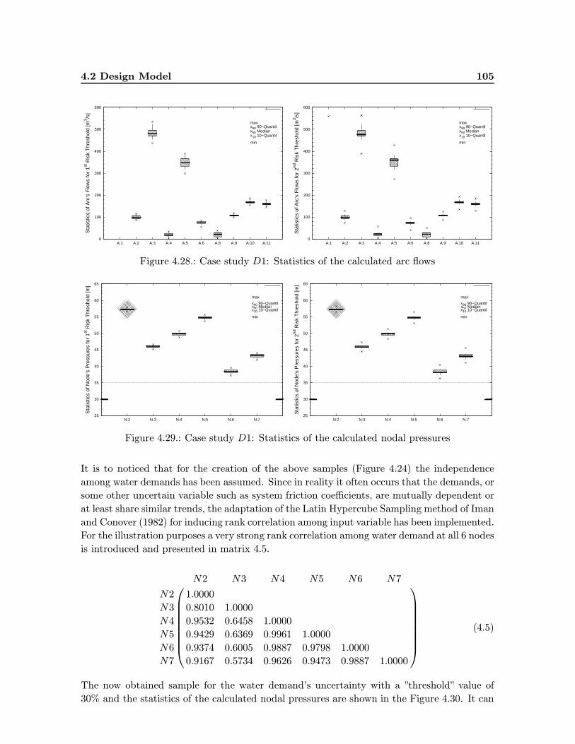
4.2 Design Model 105
0
100
200
300
400
500
600
A:1 A:2 A:3 A:4 A:5 A:6 A:8 A:9 A:10 A:11
Sta
tistic
s of
Arc
’s F
low
s fo
r 1st
Ris
k T
hres
hold
[m3 /s
]
min
x10 10−Quantilx50 Medianx90 90−Quantilmax
0
100
200
300
400
500
600
A:1 A:2 A:3 A:4 A:5 A:6 A:8 A:9 A:10 A:11
Sta
tistic
s of
Arc
’s F
low
s fo
r 2nd
Ris
k T
hres
hold
[m3 /s
]
min
x10 10−Quantilx50 Medianx90 90−Quantilmax
Figure 4.28.: Case study D1: Statistics of the calculated arc flows
25
30
35
40
45
50
55
60
65
N:2 N:3 N:4 N:5 N:6 N:7
Sta
tistic
s of
Nod
e’s
Pre
ssur
es fo
r 1st
Ris
k T
hres
hold
[m]
min
x10 10−Quantilx50 Medianx90 90−Quantil
max
25
30
35
40
45
50
55
60
65
N:2 N:3 N:4 N:5 N:6 N:7
Sta
tistic
s of
Nod
e’s
Pre
ssur
es fo
r 2nd
Ris
k T
hres
hold
[m]
min
x10 10−Quantilx50 Medianx90 90−Quantil
max
Figure 4.29.: Case study D1: Statistics of the calculated nodal pressures
It is to noticed that for the creation of the above samples (Figure 4.24) the independence
among water demands has been assumed. Since in reality it often occurs that the demands, or
some other uncertain variable such as system friction coefficients, are mutually dependent or
at least share similar trends, the adaptation of the Latin Hypercube Sampling method of Iman
and Conover (1982) for inducing rank correlation among input variable has been implemented.
For the illustration purposes a very strong rank correlation among water demand at all 6 nodes
is introduced and presented in matrix 4.5.
⎛
⎜⎜⎜⎜⎜⎜⎜⎝
N2 N3 N4 N5 N6 N7
N2 1.0000
N3 0.8010 1.0000
N4 0.9532 0.6458 1.0000
N5 0.9429 0.6369 0.9961 1.0000
N6 0.9374 0.6005 0.9887 0.9798 1.0000
N7 0.9167 0.5734 0.9626 0.9473 0.9887 1.0000
⎞
⎟⎟⎟⎟⎟⎟⎟⎠
(4.5)
The now obtained sample for the water demand’s uncertainty with a ”threshold” value of
30% and the statistics of the calculated nodal pressures are shown in the Figure 4.30. It can
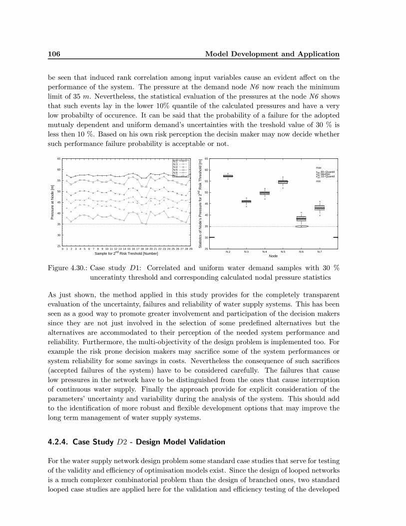
106 Model Development and Application
be seen that induced rank correlation among input variables cause an evident affect on the
performance of the system. The pressure at the demand node N6 now reach the minimum
limit of 35 m. Nevertheless, the statistical evaluation of the pressures at the node N6 shows
that such events lay in the lower 10% quantile of the calculated pressures and have a very
low probabilty of occurence. It can be said that the probability of a failure for the adopted
mutualy dependent and uniform demand’s uncertainties with the treshold value of 30 % is
less then 10 %. Based on his own risk perception the decisin maker may now decide whether
such performance failure probability is acceptable or not.
25
30
35
40
45
50
55
60
65
0 1 2 3 4 5 6 7 8 9 10 11 12 13 14 15 16 17 18 19 20 21 22 23 24 25 26 27 28 29
Pre
ssur
e at
Nod
e [m
]
Sample for 2nd Risk Treshold [Number]
N:2N:3N:4N:5N:6N:7
25
30
35
40
45
50
55
60
65
N:2 N:3 N:4 N:5 N:6 N:7
Sta
tistc
s of
Nod
e’s
Pre
ssur
e fo
r 2nd
Ris
k T
hres
hold
[m]
Node
min
x10 10−Quantilx50 Medianx90 90−Quantil
max
Figure 4.30.: Case study D1: Correlated and uniform water demand samples with 30 %
unceratinty threshold and corresponding calculated nodal pressure statistics
As just shown, the method applied in this study provides for the completely transparent
evaluation of the uncertainty, failures and reliability of water supply systems. This has been
seen as a good way to promote greater involvement and participation of the decision makers
since they are not just involved in the selection of some predefined alternatives but the
alternatives are accommodated to their perception of the needed system performance and
reliability. Furthermore, the multi-objectivity of the design problem is implemented too. For
example the risk prone decision makers may sacrifice some of the system performances or
system reliability for some savings in costs. Nevertheless the consequence of such sacrifices
(accepted failures of the system) have to be considered carefully. The failures that cause
low pressures in the network have to be distinguished from the ones that cause interruption
of continuous water supply. Finally the approach provide for explicit consideration of the
parameters’ uncertainty and variability during the analysis of the system. This should add
to the identification of more robust and flexible development options that may improve the
long term management of water supply systems.
4.2.4. Case Study D2 - Design Model Validation
For the water supply network design problem some standard case studies that serve for testing
of the validity and efficiency of optimisation models exist. Since the design of looped networks
is a much complexer combinatorial problem than the design of branched ones, two standard
looped case studies are applied here for the validation and efficiency testing of the developed
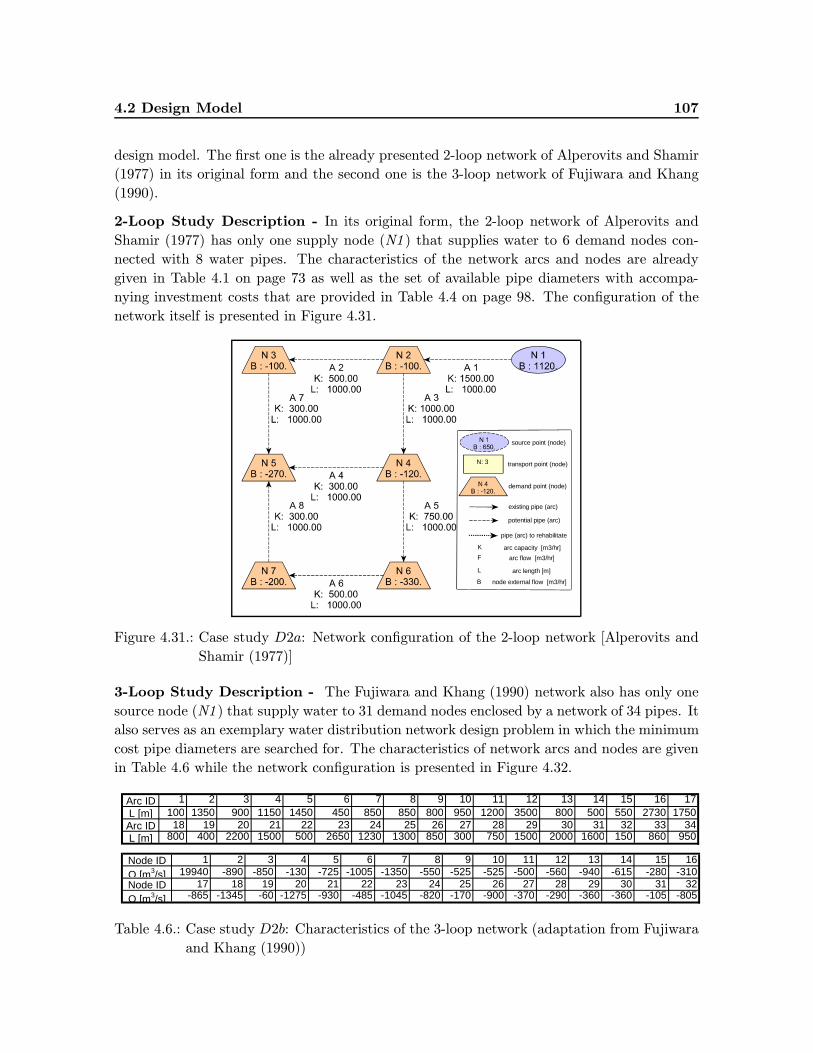
4.2 Design Model 107
design model. The first one is the already presented 2-loop network of Alperovits and Shamir
(1977) in its original form and the second one is the 3-loop network of Fujiwara and Khang
(1990).
2-Loop Study Description - In its original form, the 2-loop network of Alperovits and
Shamir (1977) has only one supply node (N1 ) that supplies water to 6 demand nodes con-
nected with 8 water pipes. The characteristics of the network arcs and nodes are already
given in Table 4.1 on page 73 as well as the set of available pipe diameters with accompa-
nying investment costs that are provided in Table 4.4 on page 98. The configuration of the
network itself is presented in Figure 4.31.
arc capacity [m3/hr]K
pipe (arc) to rehabilitate
potential pipe (arc)
existing pipe (arc)
demand point (node)
transport point (node)
source point (node)
N: 3
node external flow [m3/hr]B
arc flow [m3/hr]F
arc length [m]L
Figure 4.31.: Case study D2a: Network configuration of the 2-loop network [Alperovits and
Shamir (1977)]
3-Loop Study Description - The Fujiwara and Khang (1990) network also has only one
source node (N1 ) that supply water to 31 demand nodes enclosed by a network of 34 pipes. It
also serves as an exemplary water distribution network design problem in which the minimum
cost pipe diameters are searched for. The characteristics of network arcs and nodes are given
in Table 4.6 while the network configuration is presented in Figure 4.32.
Arc ID 1 2 3 4 5 6 7 8 9 10 11 12 13 14 15 16 17L [m] 100 1350 900 1150 1450 450 850 850 800 950 1200 3500 800 500 550 2730 1750Arc ID 18 19 20 21 22 23 24 25 26 27 28 29 30 31 32 33 34L [m] 800 400 2200 1500 500 2650 1230 1300 850 300 750 1500 2000 1600 150 860 950
Node ID 1 2 3 4 5 6 7 8 9 10 11 12 13 14 15 16
Q [m3/s] 19940 -890 -850 -130 -725 -1005 -1350 -550 -525 -525 -500 -560 -940 -615 -280 -310Node ID 17 18 19 20 21 22 23 24 25 26 27 28 29 30 31 32
Q [m3/s] -865 -1345 -60 -1275 -930 -485 -1045 -820 -170 -900 -370 -290 -360 -360 -105 -805
Table 4.6.: Case study D2b: Characteristics of the 3-loop network (adaptation from Fujiwara
and Khang (1990))
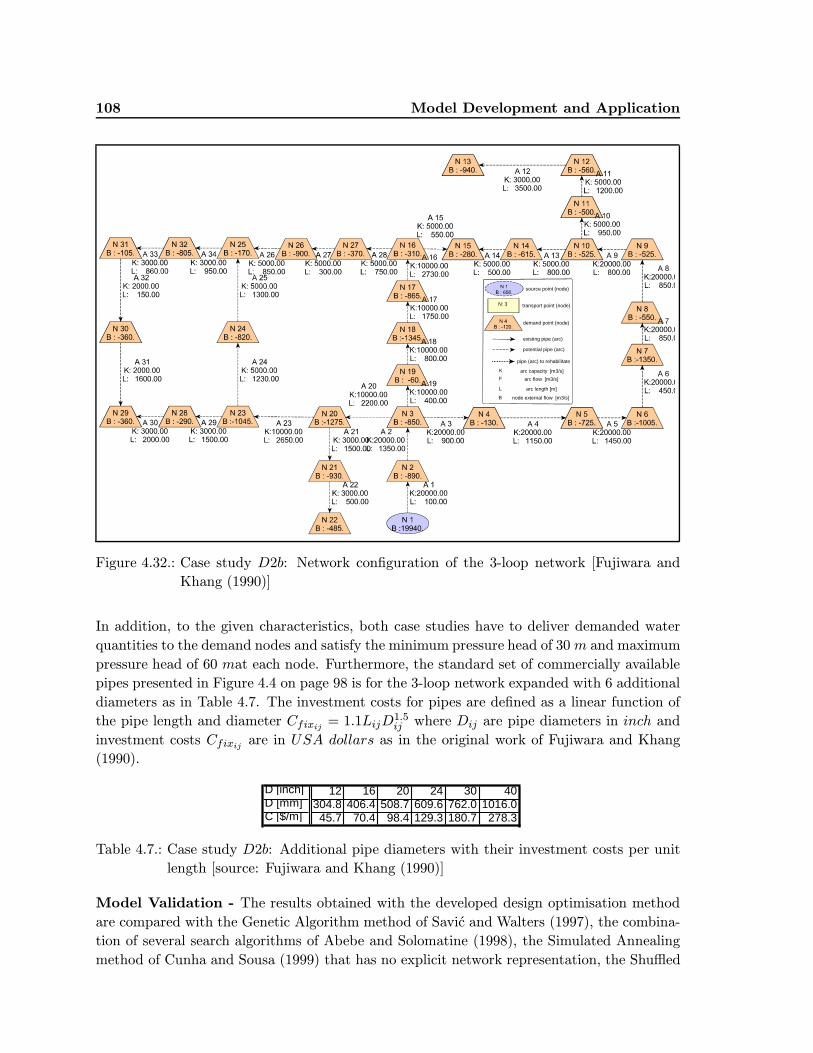
108 Model Development and Application
arc capacity [m3/s]K
pipe (arc) to rehabilitate
potential pipe (arc)
existing pipe (arc)
demand point (node)
transport point (node)
source point (node)
N: 3
node external flow [m3/s]B
arc flow [m3/s]F
arc length [m]L
Figure 4.32.: Case study D2b: Network configuration of the 3-loop network [Fujiwara and
Khang (1990)]
In addition, to the given characteristics, both case studies have to deliver demanded water
quantities to the demand nodes and satisfy the minimum pressure head of 30 m and maximum
pressure head of 60 mat each node. Furthermore, the standard set of commercially available
pipes presented in Figure 4.4 on page 98 is for the 3-loop network expanded with 6 additional
diameters as in Table 4.7. The investment costs for pipes are defined as a linear function of
the pipe length and diameter Cfixij= 1.1LijD
1.5ij where Dij are pipe diameters in inch and
investment costs Cfixijare in USA dollars as in the original work of Fujiwara and Khang
(1990).
D [inch] 12 16 20 24 30 40D [mm] 304.8 406.4 508.7 609.6 762.0 1016.0C [$/m] 45.7 70.4 98.4 129.3 180.7 278.3
Table 4.7.: Case study D2b: Additional pipe diameters with their investment costs per unit
length [source: Fujiwara and Khang (1990)]
Model Validation - The results obtained with the developed design optimisation method
are compared with the Genetic Algorithm method of Savic and Walters (1997), the combina-
tion of several search algorithms of Abebe and Solomatine (1998), the Simulated Annealing
method of Cunha and Sousa (1999) that has no explicit network representation, the Shuffled
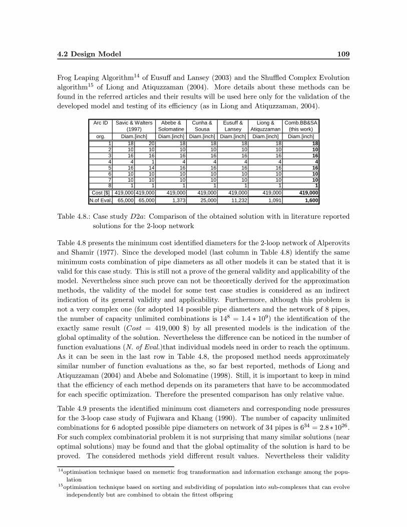
4.2 Design Model 109
Frog Leaping Algorithm14 of Eusuff and Lansey (2003) and the Shuffled Complex Evolution
algorithm15 of Liong and Atiquzzaman (2004). More details about these methods can be
found in the referred articles and their results will be used here only for the validation of the
developed model and testing of its efficiency (as in Liong and Atiquzzaman, 2004).
Arc ID Abebe & Solomatine
(1998)
Cunha & Sousa (1999)
Eusuff & Lansey (2003)
Liong & Atiquzzaman
(2004)
Comb.BB&SA (this work)
org. Diam.[inch] Diam.[inch] Diam.[inch] Diam.[inch] Diam.[inch]1 18 20 18 18 18 18 182 10 10 10 10 10 10 103 16 16 16 16 16 16 164 4 1 4 4 4 4 45 16 14 16 16 16 16 166 10 10 10 10 10 10 107 10 10 10 10 10 10 108 1 1 1 1 1 1 1
Cost [$] 419,000 419,000 419,000 419,000 419,000 419,000 419,000N.of Eval. 65,000 65,000 1,373 25,000 11,232 1,091 1,600
Diam.[inch]
Savic & Walters (1997)
Table 4.8.: Case study D2a: Comparison of the obtained solution with in literature reported
solutions for the 2-loop network
Table 4.8 presents the minimum cost identified diameters for the 2-loop network of Alperovits
and Shamir (1977). Since the developed model (last column in Table 4.8) identify the same
minimum costs combination of pipe diameters as all other models it can be stated that it is
valid for this case study. This is still not a prove of the general validity and applicability of the
model. Nevertheless since such prove can not be theoretically derived for the approximation
methods, the validity of the model for some test case studies is considered as an indirect
indication of its general validity and applicability. Furthermore, although this problem is
not a very complex one (for adopted 14 possible pipe diameters and the network of 8 pipes,
the number of capacity unlimited combinations is 148 = 1.4 ∗ 109) the identification of the
exactly same result (Cost = 419, 000 $) by all presented models is the indication of the
global optimality of the solution. Nevertheless the difference can be noticed in the number of
function evaluations (N. of Eval.)that individual models need in order to reach the optimum.
As it can be seen in the last row in Table 4.8, the proposed method needs approximately
similar number of function evaluations as the, so far best reported, methods of Liong and
Atiquzzaman (2004) and Abebe and Solomatine (1998). Still, it is important to keep in mind
that the efficiency of each method depends on its parameters that have to be accommodated
for each specific optimization. Therefore the presented comparison has only relative value.
Table 4.9 presents the identified minimum cost diameters and corresponding node pressures
for the 3-loop case study of Fujiwara and Khang (1990). The number of capacity unlimited
combinations for 6 adopted possible pipe diameters on network of 34 pipes is 634 = 2.8∗1026.For such complex combinatorial problem it is not surprising that many similar solutions (near
optimal solutions) may be found and that the global optimality of the solution is hard to be
proved. The considered methods yield different result values. Nevertheless their validity
14optimisation technique based on memetic frog transformation and information exchange among the popu-
lation15optimisation technique based on sorting and subdividing of population into sub-complexes that can evolve
independently but are combined to obtain the fittest offspring

110 Model Development and Application
Arc ID Abebe & Solomatine
(1998)
Cunha & Sousa (1999)
Liong & Atiquzzaman (2004)
Combination of BB & SA (this work)
org. D.[inch] D.[inch] D.[inch] D.[inch]
1 40 40 40 40 40 402 40 40 40 40 40 403 40 40 40 40 40 404 40 40 40 40 40 405 40 40 30 40 40 406 40 40 40 40 40 407 40 40 40 40 40 408 40 40 30 40 30 309 40 30 30 40 30 30
10 30 30 30 30 30 3011 24 30 30 24 30 3012 24 24 30 24 24 2413 20 16 16 20 16 1614 16 16 24 16 12 1215 12 12 30 12 12 1216 12 16 30 12 24 3017 16 20 30 16 30 3018 20 24 40 20 30 3019 20 24 40 20 30 3020 40 40 40 40 40 4021 20 20 20 20 20 2022 12 12 20 12 12 1223 40 40 30 40 30 3024 30 30 16 30 30 2425 30 30 20 30 24 2026 20 20 12 20 12 1627 12 12 24 12 20 2028 12 12 20 12 24 2429 16 16 24 16 16 1630 16 16 30 12 16 1631 12 12 30 12 12 1232 12 12 30 16 16 1233 16 16 30 16 20 2034 20 20 12 24 24 24
Cost [M.$] 6,073 6,195 7,000 6,056 6,220 6,270N.of Eval. - - 16,910 53,000 25,402 19,000
Savic & Walters (1997)
D.[inch]
Node ID Abebe & Solomatine
(1998)
Cunha & Sousa (1999)
Liong & Atiquzzaman (2004)
Combination of BB & SA (this work)
org. D.[inch] D.[inch] D.[inch] D.[inch]
1 100 100 100 100 100 1002 97.14 97.14 97.14 97.14 97.14 97.143 61.63 61.63 61.67 61.63 61.67 61.674 56.83 57.26 58.59 56.82 57.54 57.635 50.89 51.86 54.82 50.86 52.43 52.646 44.62 46.21 39.45 44.57 47.13 47.467 43.14 44.91 38.65 43.1 45.92 46.298 41.38 43.4 37.87 41.33 44.55 44.979 39.97 42.23 35.65 39.91 40.27 40.88
10 38.93 38.79 34.28 38.86 37.24 38.0111 37.37 37.23 32.72 37.3 35.68 36.4512 33.94 36.07 31.56 33.87 34.52 35.2913 29.72* 31.86 30.13 29.66* 30.32 31.0814 35.06 33.19 36.36 34.94 34.08 35.6415 33.07 32.9 37.17 32.88 34.08 35.8516 30.15 33.01 37.63 29.79* 36.13 39.2717 30.24 40.73 48.11 29.95* 48.64 45.4218 43.91 51.13 58.62 43.81 54 52.4419 55.53 58.03 60.64 55.49 59.07 58.5420 50.39 50.63 53.87 50.43 53.62 54.4021 41.03 41.28 44.48 41.07 44.27 45.1122 35.86 36.11 44.05 35.9 39.11 39.9523 44.15 44.61 39.83 44.24 38.79 41.9524 38.84 39.54 30.51 38.5 36.37 37.1325 35.48 36.4 30.5 34.79 33.16 33.2226 31.46 32.93 32.14 30.87 33.44 34.9327 30.03 32.18 32.62 29.59* 34.38 36.5728 35.43 36.02 33.52 38.6 32.64 34.3129 30.67 31.38 31.46 29.64* 30.05 30.4930 29.65* 30.47 30.44 29.90* 30.1 30.2031 30.12 30.95 30.39 30.18 30.35 30.8532 31.36 32.24 30.17 32.64 31.09 31.35
Cost [M.$] 6,073 6,195 7,000 6,056 6,220 6,270N.of Eval. - - 16,910 53,000 25,402 19,000
D.[inch]
Savic and Walters (1997)
Table 4.9.: Case study D2b: Comparison of the obtained solution with in literature reported
solutions for the 3-loop network
and efficiency can be compared on the basis of identified solution values together with the
needed number of function evaluations. In this respect, the developed method (last column
in Table 4.9) manages to identify solution that is on the lower side of the needed function
evaluations (N.of Eval.) and still has a very good minimum cost result (Cost = 6, 270M$).
Additionally it is to be noticed that the minimum pressure of 30 m at all nodes present an
additional limiting constraint that is not fully obeyed by all presented method (pressures
under 30 m are marked with * in Table 4.9) but is satisfied by the here calculated solution.
Model Sensitivity - As just mentioned, the minimum pressure constraint has a very large
influence on the final result of the optimisation procedure. In order to test and quantify this
statement 4 new optimisation runs are made with the relaxed minimum pressure constraint.
The results are shown in Figure 4.33. It can be seen that the optimisation procedure manage
to identify the lower cost solutions for the weaker minimum pressure constraint scenarios.
Although the relative improvements are quite modest (approximately 1 % of cost savings for
1 m lower pressure constraint), the possiblity to identify different solutions that are optimal
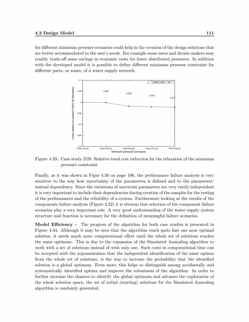
4.2 Design Model 111
for different minimum pressure scenarios could help in the creation of the design solutions that
are better accommodated to the user’s needs. For example some users and decisio makers may
readily trade-off some savings in economic costs for lower distributed pressures. In addition
with the developed model it is possible to define different minimum pressure constraint for
different parts, or zones, of a water supply network.
0.8
0.85
0.9
0.95
1
1.05
1.1
Pmin=30 [m] Pmin=29 [m] Pmin=28 [m] Pmin=27 [m] Pmin=26 [m]
Cos
ts r
elat
ive
to s
olut
ion
Pm
in=
30 [N
umbe
r]
Minimum pressure scenarios
0.9990.982
0.9780.977
relative costs
Figure 4.33.: Case studyD2b: Relative total cost reduction for the relaxation of the minimum
pressure constraint
Finally, as it was shown in Figur 4.30 on page 106, the performance failure analysis is very
sensitive to the way how uncertainty of the parameters is defined and to the parameters’
mutual dependency. Since the variations of uncertain parameters are very rarely independent
it is very important to include their dependencies during creation of the samples for the testing
of the performances and the reliability of a system. Furthermore looking at the results of the
components failure analysis (Figure 4.22) it is obvious that selection of the component failure
scenarios play a very important role. A very good understanding of the water supply system
structure and function is necessary for the definition of meaningful failure scenarios.
Model Efficiency - The progress of the algorithm for both case studies is presented in
Figure 4.34. Although it may be seen that the algorithm reach quite fast one near optimal
solution, it needs much more computational effort until the whole set of solutions reaches
the same optimum. This is due to the expansion of the Simulated Annealing algorithm to
work with a set of solutions instead of with only one. Such costs in computational time can
be accepted with the argumentation that the independent identification of the same optima
from the whole set of solutions, is the way to increase the probability that the identified
solution is a global optimum. Even more, this helps to distinguish among accidentally and
systematically identified optima and improve the robustness of the algorithm. In order to
further increase the chances to identify the global optimum and advance the exploration of
the whole solution space, the set of initial (starting) solutions for the Simulated Annealing
algorithm is randomly generated.
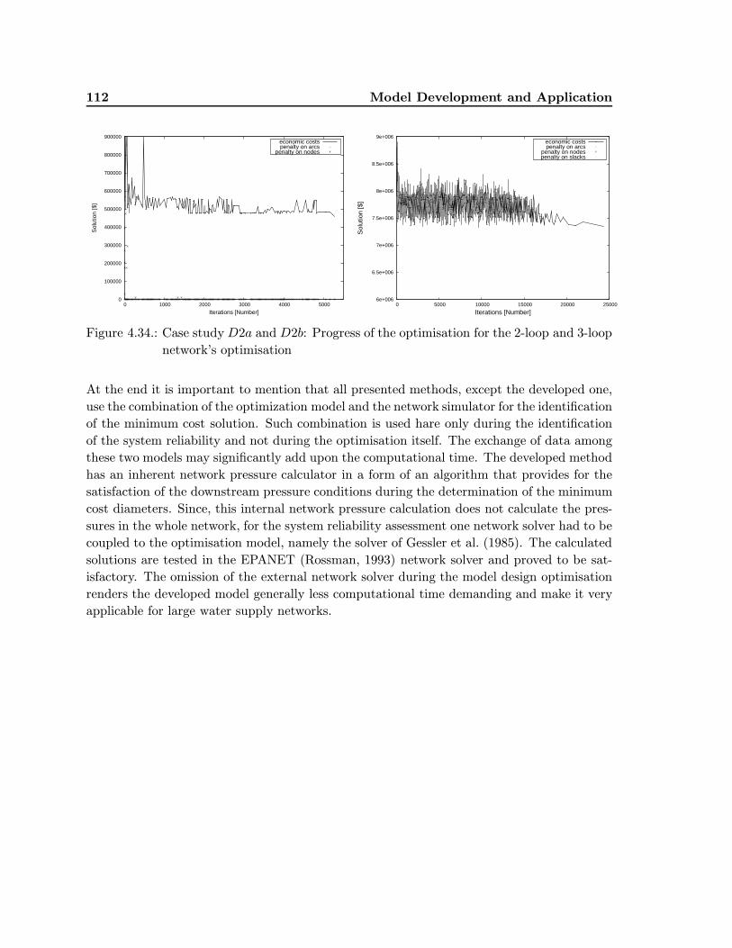
112 Model Development and Application
0
100000
200000
300000
400000
500000
600000
700000
800000
900000
0 1000 2000 3000 4000 5000
Sol
utio
n [$
]
Iterations [Number]
economic costspenalty on arcs
penalty on nodes
6e+006
6.5e+006
7e+006
7.5e+006
8e+006
8.5e+006
9e+006
0 5000 10000 15000 20000 25000
Sol
utio
n [$
]
Iterations [Number]
economic costspenalty on arcs
penalty on nodespenalty on slacks
Figure 4.34.: Case studyD2a and D2b: Progress of the optimisation for the 2-loop and 3-loop
network’s optimisation
At the end it is important to mention that all presented methods, except the developed one,
use the combination of the optimization model and the network simulator for the identification
of the minimum cost solution. Such combination is used hare only during the identification
of the system reliability and not during the optimisation itself. The exchange of data among
these two models may significantly add upon the computational time. The developed method
has an inherent network pressure calculator in a form of an algorithm that provides for the
satisfaction of the downstream pressure conditions during the determination of the minimum
cost diameters. Since, this internal network pressure calculation does not calculate the pres-
sures in the whole network, for the system reliability assessment one network solver had to be
coupled to the optimisation model, namely the solver of Gessler et al. (1985). The calculated
solutions are tested in the EPANET (Rossman, 1993) network solver and proved to be sat-
isfactory. The omission of the external network solver during the model design optimisation
renders the developed model generally less computational time demanding and make it very
applicable for large water supply networks.
4.3 Operation Model 113
4.3. Operation Model
Some of the aims of the analysis of the water supply systems’ operation are to secure tech-
nical functioning of the systems, to provide the satisfaction of user’s demands, to fulfil the
regulatory criteria and engineering standards in terms of systems performances and services,
to provide for system maintenance and further development, etc.. Obviously, for the achieve-
ment of all these aims, the operation analysis has to be done already during planning and
design management stages. Only when incorporated in these early phases of water supply
systems management the stated objectives of the system operation can be achieved later on
(Walski et al., 2003).
4.3.1. Characterisation of the Operation Problem
In contrary to the design optimisation, which focuses on the worst stress conditions, the op-
eration analysis primarily considers normal, or every day, operation conditions. Furthermore,
the ”steady-state analysis” for one specific point in time is not sufficient any more and the,
so called, ”extended period simulation” has to be done. This is actually the simulation of
the system behaviour during some preselected time period. It enables the analysis of the
components that transfer water in time, such as tanks and reservoirs, dimensioning of their
capacities and definition of their operation rules. In addition, it provides for the creation of
the operation rules for all manageable system components such as pumps, valves, pressure
reducers, etc. Although each operation analysis is very case specific, from the engineering
point of view following objectives can be stated:
1. Performance satisfaction.
2. Minimization of the investment costs for water storage elements.
3. Minimization of the operation costs for pump stations.
In addition to the performance indicators defined in the design phase (i.e. flows and pres-
sures), the extended period simulation allows for the calculation of the water residual time
and the volume exchange time in tanks and reservoirs. These indicators are the basis for
the analysis of the water quality in water supply networks but since this study deal with the
water quantity issues only, they will not be further considered. The performance indicators
for the operation optimisation analysis are restricted to delivered flows, nodal pressures and
volume exchange time in tanks.
As far as the second and third objectives are concerned, an additional restriction had to
be introduced. Although for the majority of water supply systems the major part of the
operation costs are the energy costs for water elevation and pumping, the exceptions are the
systems that exclusively use gravity water flow. Operation costs mainly originate from the
need to transport water along network and from the need to equalise temporal variation of
water demands. Tanks and reservoirs are the elements that enable temporal redistribution
of water by storing it in time. Since tanks also serve for the control and stabilisation of the
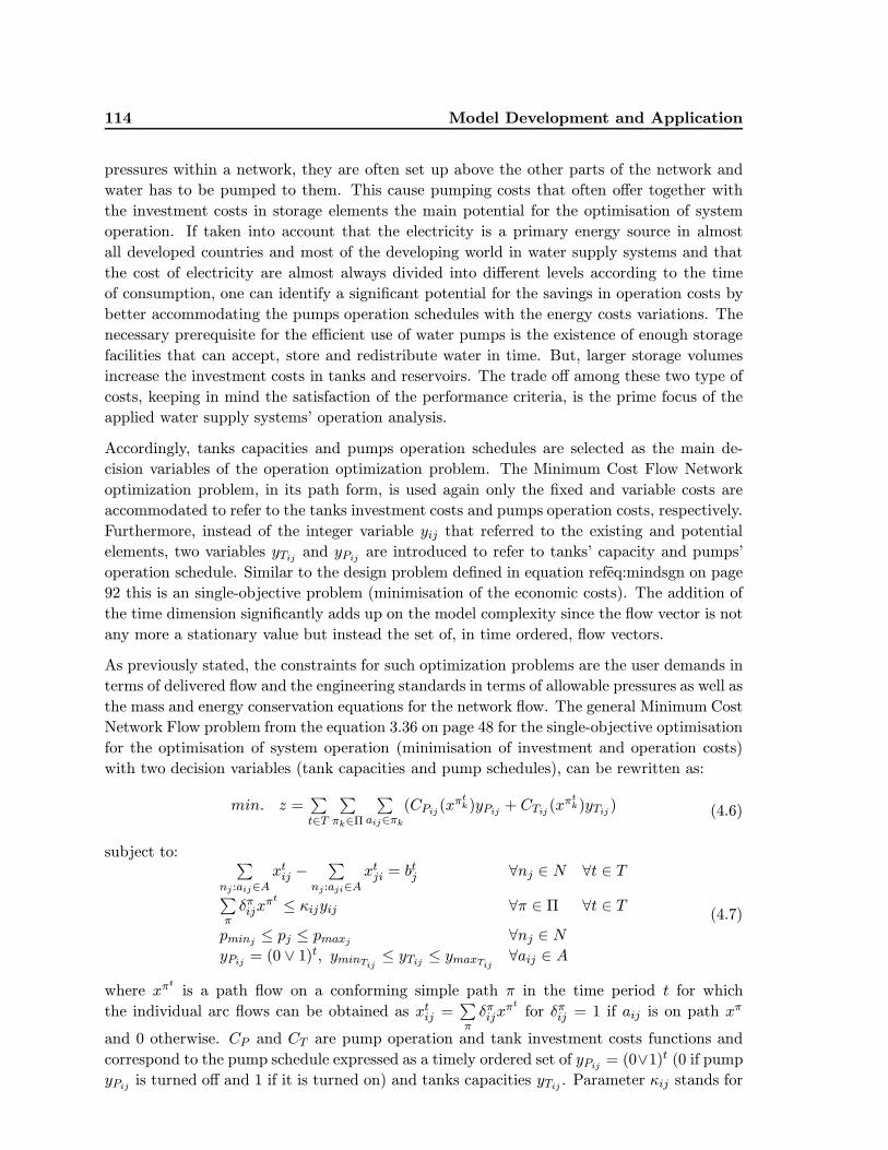
114 Model Development and Application
pressures within a network, they are often set up above the other parts of the network and
water has to be pumped to them. This cause pumping costs that often offer together with
the investment costs in storage elements the main potential for the optimisation of system
operation. If taken into account that the electricity is a primary energy source in almost
all developed countries and most of the developing world in water supply systems and that
the cost of electricity are almost always divided into different levels according to the time
of consumption, one can identify a significant potential for the savings in operation costs by
better accommodating the pumps operation schedules with the energy costs variations. The
necessary prerequisite for the efficient use of water pumps is the existence of enough storage
facilities that can accept, store and redistribute water in time. But, larger storage volumes
increase the investment costs in tanks and reservoirs. The trade off among these two type of
costs, keeping in mind the satisfaction of the performance criteria, is the prime focus of the
applied water supply systems’ operation analysis.
Accordingly, tanks capacities and pumps operation schedules are selected as the main de-
cision variables of the operation optimization problem. The Minimum Cost Flow Network
optimization problem, in its path form, is used again only the fixed and variable costs are
accommodated to refer to the tanks investment costs and pumps operation costs, respectively.
Furthermore, instead of the integer variable yij that referred to the existing and potential
elements, two variables yTij and yPij are introduced to refer to tanks’ capacity and pumps’
operation schedule. Similar to the design problem defined in equation refeq:mindsgn on page
92 this is an single-objective problem (minimisation of the economic costs). The addition of
the time dimension significantly adds up on the model complexity since the flow vector is not
any more a stationary value but instead the set of, in time ordered, flow vectors.
As previously stated, the constraints for such optimization problems are the user demands in
terms of delivered flow and the engineering standards in terms of allowable pressures as well as
the mass and energy conservation equations for the network flow. The general Minimum Cost
Network Flow problem from the equation 3.36 on page 48 for the single-objective optimisation
for the optimisation of system operation (minimisation of investment and operation costs)
with two decision variables (tank capacities and pump schedules), can be rewritten as:
min. z =∑
t∈T
∑
πk∈Π
∑
aij∈πk
(CPij (xπtk)yPij + CTij (x
πtk)yTij ) (4.6)
subject to: ∑
nj :aij∈Axtij −
∑
nj :aji∈Axtji = btj ∀nj ∈ N ∀t ∈ T
∑
πδπijx
πt ≤ κijyij ∀π ∈ Π ∀t ∈ T
pminj ≤ pj ≤ pmaxj ∀nj ∈ N
yPij = (0 ∨ 1)t, yminTij≤ yTij ≤ ymaxTij
∀aij ∈ A
(4.7)
where xπtis a path flow on a conforming simple path π in the time period t for which
the individual arc flows can be obtained as xtij =∑
πδπijx
πtfor δπij = 1 if aij is on path xπ
and 0 otherwise. CP and CT are pump operation and tank investment costs functions and
correspond to the pump schedule expressed as a timely ordered set of yPij = (0∨1)t (0 if pump
yPij is turned off and 1 if it is turned on) and tanks capacities yTij . Parameter κij stands for
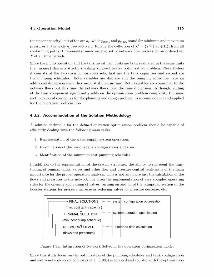
4.3 Operation Model 115
the upper capacity limit of the arc aij while pminj and pmaxj stand for minimum and maximum
pressures at the node nj, respectively. Finally the collection of xt = {xπtk | πk ∈ Π}, from all
conforming paths Π, represents timely ordered set of network flow vectors for an ordered set
T of all time periods.
Since the pump operation and the tank investment costs are both evaluated in the same units
(i.e. money) this is a strictly speaking single-objective optimization problem. Nevertheless
it consists of the two decision variables sets, first are the tank capacities and second are
the pumping schedules. Both variables are discrete and the pumping schedules have an
additional dimension since they are distributed in time. Both variables are connected to the
network flows but this time the network flows have the time dimension. Although, adding
of the time component significantly adds on the optimisation problem complexity the same
methodological concept as for the planning and design problem, is accommodated and applied
for the operation problem, too.
4.3.2. Accommodation of the Solution Methodology
A solution technique for the defined operation optimization problem should be capable of
efficiently dealing with the following main tasks:
1. Representation of the water supply system operation.
2. Examination of the various tank configurations and sizes.
3. Identification of the minimum cost pumping schedules.
In addition to the representation of the system structure, the ability to represent the func-
tioning of pumps, tanks, valves and other flow and pressure control facilities is of the main
importance for the proper operation analysis. This is not any more just the calculation of the
flows and pressures in the network but often the implementation of very complex operating
rules for the opening and closing of valves, turning on and off of the pumps, activation of the
booster stations for pressure increase or reducing valves for pressure decrease, etc.
PRIMAL SOLUTION
(min. cost pump schedule)
FINAL SOLUTIONS
(min. cost tank capacity )
system operation optimisation
system configuration optimisation
NETWORK SOLVER
(flows and pressures)
extended time calculation
Figure 4.35.: Integration of Network Solver in the operation optimisation model
Since this study focus on the optimization of the pumping schedules and tank configuration
and size, a network solver of Gessler et al. (1985) is adopted and coupled with the optimisation

116 Model Development and Application
model for the calculation of network flows, pressures and tank levels during the extended
period simulation as in Figure 4.35.
The optimization solution procedure consists of the following steps (Figure 4.36):
1. Input - Beside basic data about a water supply system (i.e. configuration, layout,
capacities, supplies, demands, hydraulic properties, etc.) the data for the temporal
water distribution have to be defined, too. These are mainly the position, available
volumes, and operation water levels of tanks and reservoirs as well as the position
and characteristics of pumps and pressure reducing valves. In addition, investment
costs of the new elements or elements that can be rehabilitated as well as the energy
cost of pump operation have to be provided. Finally the time period for which the
extended period simulation is to be done, have to be defined. It depends on the system
characteristics and size but it is mainly defined as the period for which the tanks cover
the consumption variation (normally 24 hours or daily demand variation).
2. Primal solution - system operation optimization - The Simulated Annealing algorithm
is used to identify the minimum cost pump operation schedule for one system configu-
ration with predefined tank and reservoir volumes. The algorithm iteratively produces
random pumping schedules, calculate energy usage and corresponding costs and accepts
or rejects solutions based on the metropolis schedule. The identification of the network
flows and pressures at each time step of the extended period simulation is done by the
network solver of Gessler et al. (1985). Identified minimum cost solution is referred as
the primal solution and is used as the reference point for the identification of possible
operation savings by investing in tank and reservoir expansion or building of some new
storage elements.
3. Final solutions - system configuration optimization - The Branch and Bound algorithm
is used to question different combinations of tank and reservoir volumes and the above
described Simulated Annealing procedure to identify the minimum cost operation sched-
ule for each combination. The total costs (sum of investment and operation costs) are
calculated and compared until the minimum cost configuration is found. In order to
avoid analysis of all possible combinations of new elements, the algorithm sorts differ-
ent combinations of tanks and reservoirs with their possible volumes in a tree ordered
structure that enable omission, so called ”fathoming”, of configurations that are only
refinements of the already examined ones. Since the investment and operation costs
are referred to the primal solution (costs are divided with the corresponding costs of
the primal solution) the progress of the algorithm can be easily followed. The finally
identified solution is a trade off among tank investments and pump operation costs that
yield a minim total costs for a given operation period.
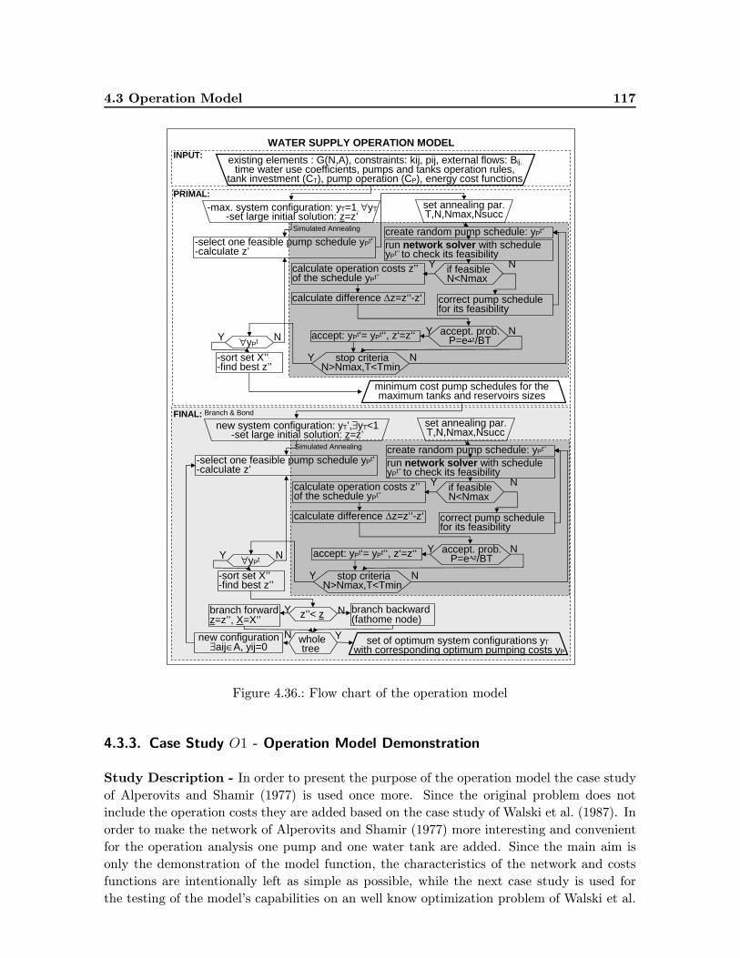
4.3 Operation Model 117
Y
-max. system configuration: yT=1, ∀yT-set large initial solution: z=z’
create random pump schedule: yPt’’
correct pump schedulefor its feasibility
accept. prob.P=e∆z/BT
set annealing par.T,N,Nmax,Nsucc
calculate difference ∆z=z‘‘-z‘
Naccept: yPt‘= yPt‘‘, z‘=z‘‘
Y stop criteriaN>Nmax,T<Tmin
N
-select one feasible pump schedule yPt’-calculate z’
Y ∀yPt N
-sort set X’’-find best z’’
PRIMAL:
Simulated Annealing
FINAL: Branch & Bond
WATER SUPPLY OPERATION MODEL
existing elements : G(N,A), constraints: kij, pij, external flows: Bij, time water use coefficients, pumps and tanks operation rules,
tank investment (CT), pump operation (CP), energy cost functions
INPUT:
run network solver with scheduleyPt’’ to check its feasibility
calculate operation costs z’’of the schedule yPt’’
Y if feasibleN<Nmax
N
minimum cost pump schedules for the maximum tanks and reservoirs sizes
Y
new system configuration: yT’,∃yT<1-set large initial solution: z=z’
create random pump schedule: yPt’’
correct pump schedulefor its feasibility
accept. prob.P=e∆z/BT
set annealing par.T,N,Nmax,Nsucc
calculate difference ∆z=z‘‘-z‘
Naccept: yPt‘= yPt‘‘, z‘=z‘‘
Y stop criteriaN>Nmax,T<Tmin
N
Y z’’< z N
-select one feasible pump schedule yPt’-calculate z’
Y ∀yPt N
-sort set X’’-find best z’’
branch forwardz=z’’, X=X’’
branch backward(fathome node)
N wholetree
Ynew configuration∃aij∈A, yij=0
set of optimum system configurations yTwith corresponding optimum pumping costs yP
Simulated Annealing
run network solver with scheduleyPt’’ to check its feasibility
calculate operation costs z’’of the schedule yPt’’
Y if feasibleN<Nmax
N
Figure 4.36.: Flow chart of the operation model
4.3.3. Case Study O1 - Operation Model Demonstration
Study Description - In order to present the purpose of the operation model the case study
of Alperovits and Shamir (1977) is used once more. Since the original problem does not
include the operation costs they are added based on the case study of Walski et al. (1987). In
order to make the network of Alperovits and Shamir (1977) more interesting and convenient
for the operation analysis one pump and one water tank are added. Since the main aim is
only the demonstration of the model function, the characteristics of the network and costs
functions are intentionally left as simple as possible, while the next case study is used for
the testing of the model’s capabilities on an well know optimization problem of Walski et al.
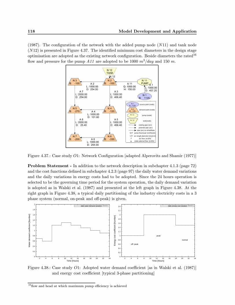
118 Model Development and Application
(1987). The configuration of the network with the added pump node (N11) and tank node
(N12) is presented in Figure 4.37. The identified minimum cost diameters in the design stage
optimisation are adopted as the existing network configuration. Beside diameters the rated16
flow and pressure for the pump A11 are adopted to be 1000 m3/day and 150 m.
demand point (node)
pump (node)
source point (node)
N: 11
pump flow,head [m3/hr],[m]Q,H
pipe (arc) to rehabilitate
potential pipe (arc)
existing pipe (arc)
node external flow [m3/hr]B
arc flow [m3/hr]F
L,D arc length,diameter [m],[mm]
tank(node)N: 12
Figure 4.37.: Case study O1: Network Configuration [adapted Alperovits and Shamir (1977)]
Problem Statement - In addition to the network description in subchapter 4.1.3 (page 72)
and the cost functions defined in subchapter 4.2.3 (page 97) the daily water demand variations
and the daily variations in energy costs had to be adopted. Since the 24 hours operation is
selected to be the governing time period for the system operation, the daily demand variation
is adopted as in Walski et al. (1987) and presented at the left graph in Figure 4.38. At the
right graph in Figure 4.38, a typical daily partitioning of the industry electricity costs in a 3
phase system (normal, on-peak and off-peak) is given.
0
0.2
0.4
0.6
0.8
1
1.2
1.4
1.6
1.8
2
2 4 6 8 10 12 14 16 18 20 22 24
Wat
er d
eman
d co
effic
ient
[Num
ber]
Time [Hours]
daily water demand variation
0
0.2
0.4
0.6
0.8
1
1.2
1.4
1.6
1.8
2
2.2
2.4
2 4 6 8 10 12 14 16 18 20 22 24
Ene
rgy
cost
coe
ffici
ent [
Num
ber]
Time [Hours]
off−peak
peak
normal
daily energy cost variation
Figure 4.38.: Case study O1: Adopted water demand coefficient [as in Walski et al. (1987)]
and energy cost coefficient [typical 3-phase partitioning]
16flow and head at which maximum pump efficiency is achieved
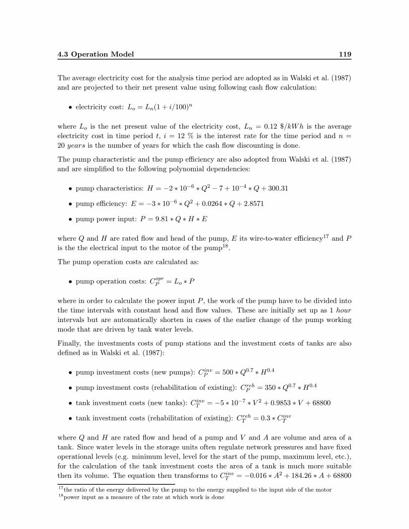
4.3 Operation Model 119
The average electricity cost for the analysis time period are adopted as in Walski et al. (1987)
and are projected to their net present value using following cash flow calculation:
• electricity cost: Lo = Ln(1 + i/100)n
where Lo is the net present value of the electricity cost, Ln = 0.12 $/kWh is the average
electricity cost in time period t, i = 12 % is the interest rate for the time period and n =
20 years is the number of years for which the cash flow discounting is done.
The pump characteristic and the pump efficiency are also adopted from Walski et al. (1987)
and are simplified to the following polynomial dependencies:
• pump characteristics: H = −2 ∗ 10−6 ∗Q2 − 7 + 10−4 ∗Q+ 300.31
• pump efficiency: E = −3 ∗ 10−6 ∗Q2 + 0.0264 ∗Q+ 2.8571
• pump power input: P = 9.81 ∗Q ∗H ∗ E
where Q and H are rated flow and head of the pump, E its wire-to-water efficiency17 and P
is the the electrical input to the motor of the pump18.
The pump operation costs are calculated as:
• pump operation costs: CoprP = Lo ∗ P
where in order to calculate the power input P , the work of the pump have to be divided into
the time intervals with constant head and flow values. These are initially set up as 1 hour
intervals but are automatically shorten in cases of the earlier change of the pump working
mode that are driven by tank water levels.
Finally, the investments costs of pump stations and the investment costs of tanks are also
defined as in Walski et al. (1987):
• pump investment costs (new pumps): CinvP = 500 ∗Q0.7 ∗H0.4
• pump investment costs (rehabilitation of existing): CrehP = 350 ∗Q0.7 ∗H0.4
• tank investment costs (new tanks): CinvT = −5 ∗ 10−7 ∗ V 2 + 0.9853 ∗ V + 68800
• tank investment costs (rehabilitation of existing): CrehT = 0.3 ∗ Cinv
T
where Q and H are rated flow and head of a pump and V and A are volume and area of a
tank. Since water levels in the storage units often regulate network pressures and have fixed
operational levels (e.g. minimum level, level for the start of the pump, maximum level, etc.),
for the calculation of the tank investment costs the area of a tank is much more suitable
then its volume. The equation then transforms to CinvT = −0.016 ∗ A2 + 184.26 ∗ A + 68800
17the ratio of the energy delivered by the pump to the energy supplied to the input side of the motor18power input as a measure of the rate at which work is done
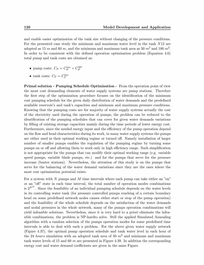
120 Model Development and Application
and enable easier optimization of the tank size without changing of the pressure conditions.
For the presented case study the minimum and maximum water level in the tank N12 are
adopted as 15 m and 60 m, and the minimum and maximum tank area as 50 m2 and 100 m2.
In order to be consistent with the defined operation optimisation problem (Equation 4.6)
total pump and tank costs are obtained as:
• pump costs: CP = CinvP + Copr
P
• tank costs: CT = CinvT
Primal solution - Pumping Schedule Optimisation - From the operation point of view
the most cost demanding elements of water supply systems are pump stations. Therefore
the first step of the optimization procedure focuses on the identification of the minimum
cost pumping schedule for the given daily distribution of water demands and the predefined
available reservoir’s and tank’s capacities and minimum and maximum pressure conditions.
Knowing that the pumping costs are for majority of water supply systems actually the cost
of the electricity used during the operation of pumps, the problem can be reduced to the
identification of the pumping schedules that can cover for given water demands variations
by filling of existing storage capacities mainly during the time periods of lower energy cost.
Furthermore, since the needed energy input and the efficiency of the pump operation depend
on the flow and head characteristics during its work, in many water supply systems the pumps
are either used in their optimal working regime or turned off. Namely installation of larger
number of smaller pumps enables the regulation of the pumping regime by turning some
pumps on or off and allowing them to work only in high efficiency range. Such simplification
is not appropriate for the pumps that can modify their optimal working range (e.g. variable
speed pumps, variable blade pumps, etc.) and for the pumps that serve for the pressure
increase (buster stations). Nevertheless, the attention of this study is on the pumps that
serve for the balancing of the water demand variations since they are the ones where the
most cost optimisation potential exists.
For a system with N pumps and M time intervals where each pump can take either an ”on”
or an ”off” state in each time interval, the total number of operation modes combinations
is 2NM. Since the feasibility of an individual pumping schedule depends on the water levels
in its controlling water tank (for pressure controlled pumps reaching of a certain boundary
head on some predefined network nodes causes either start or stop of the pump operation)
and the feasibility of the whole schedule depends on the satisfaction of the water demands
and nodal pressures in the whole network, many of the pumps operation combinations will
yield infeasible solutions. Nevertheless, since it is very hard to a priori eliminate the infea-
sible combinations, the problem is NP-hardto solve. Still the applied Simulated Annealing
algorithm with a random selection of the pumps operation modes for some predefined time
intervals is able to deal with such a problem. For the above given water supply network
(Figure 4.37), the optimal pump operation schedule and tank water level in each hour of
the 24 hours simulation with an adopted tank area of 50 m2 and minimum and maximum
tank water levels of 15 and 60 m are presented in Figure 4.39. In addition the corresponding
energy cost and water demand coefficients are given in the same Figure.
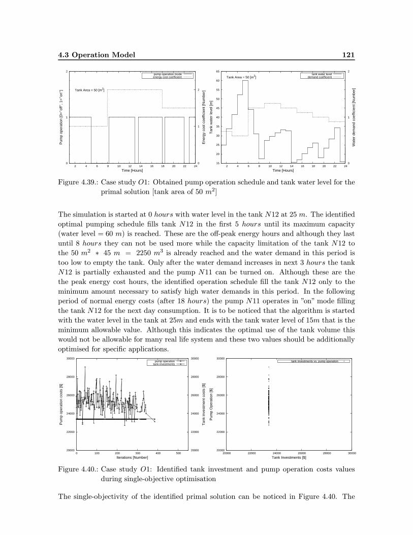
4.3 Operation Model 121
0
1
2
2 4 6 8 10 12 14 16 18 20 22 24 0
1
2
Pum
p op
erat
ion
[0=
’’off’
’, 1=
’’on’
’]
Ene
rgy
cost
coe
ffici
ent [
Num
ber]
Time [Hours]
Tank Area = 50 [m2]
pump operation modeenergy cost coefficient
15
20
25
30
35
40
45
50
55
60
65
2 4 6 8 10 12 14 16 18 20 22 24 0
1
2
Tan
k w
ater
leve
l [m
]
Wat
er d
eman
d co
effic
ient
[Num
ber]
Time [Hours]
Tank Area = 50 [m2]tank water level
demand coefficient
Figure 4.39.: Case study O1: Obtained pump operation schedule and tank water level for the
primal solution [tank area of 50 m2]
The simulation is started at 0 hours with water level in the tank N12 at 25 m. The identified
optimal pumping schedule fills tank N12 in the first 5 hours until its maximum capacity
(water level = 60 m) is reached. These are the off-peak energy hours and although they last
until 8 hours they can not be used more while the capacity limitation of the tank N12 to
the 50 m2 ∗ 45 m = 2250 m3 is already reached and the water demand in this period is
too low to empty the tank. Only after the water demand increases in next 3 hours the tank
N12 is partially exhausted and the pump N11 can be turned on. Although these are the
the peak energy cost hours, the identified operation schedule fill the tank N12 only to the
minimum amount necessary to satisfy high water demands in this period. In the following
period of normal energy costs (after 18 hours) the pump N11 operates in ”on” mode filling
the tank N12 for the next day consumption. It is to be noticed that the algorithm is started
with the water level in the tank at 25m and ends with the tank water level of 15m that is the
minimum allowable value. Although this indicates the optimal use of the tank volume this
would not be allowable for many real life system and these two values should be additionally
optimised for specific applications.
20000
22000
24000
26000
28000
30000
0 100 200 300 400 500 20000
22000
24000
26000
28000
30000
Pum
p op
erat
ion
cost
s [$
]
Tan
k in
vest
men
t cos
ts [$
]
Iterations [Number]
pump operationtank investments
20000
22000
24000
26000
28000
30000
20000 22000 24000 26000 28000 30000
Pum
p O
pera
tion
[$]
Tank Investments [$]
tank investments vs. pump operation
Figure 4.40.: Case study O1: Identified tank investment and pump operation costs values
during single-objective optimisation
The single-objectivity of the identified primal solution can be noticed in Figure 4.40. The
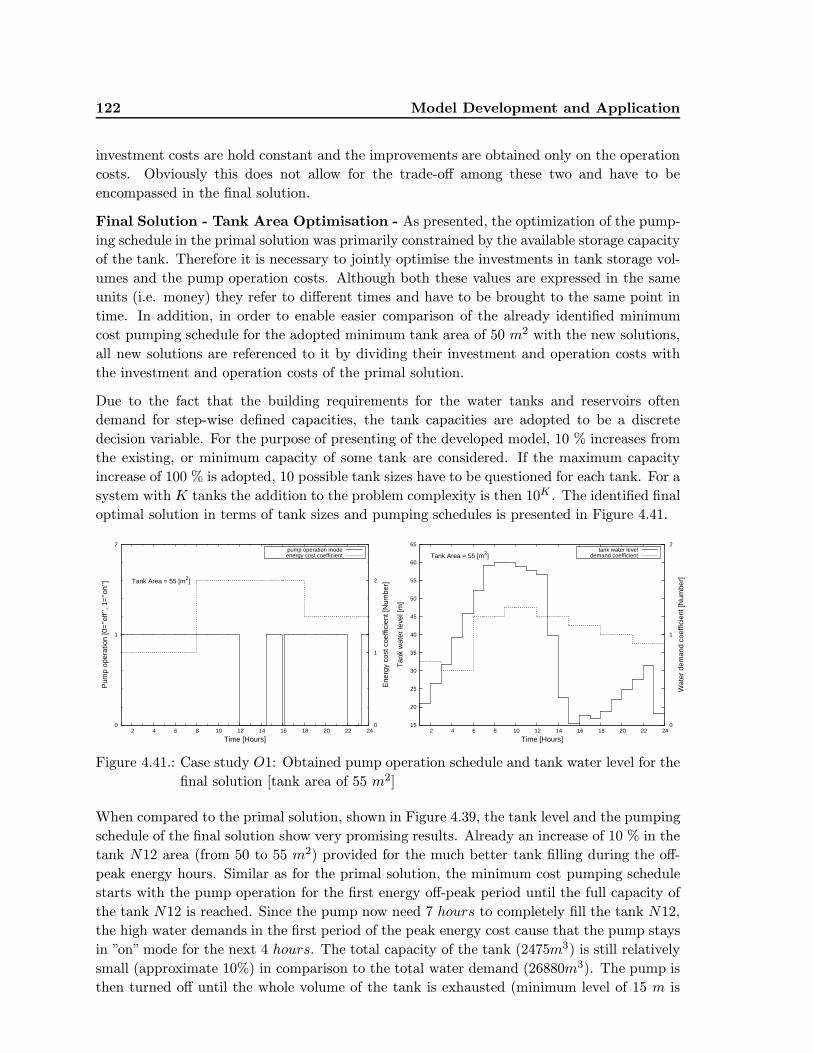
122 Model Development and Application
investment costs are hold constant and the improvements are obtained only on the operation
costs. Obviously this does not allow for the trade-off among these two and have to be
encompassed in the final solution.
Final Solution - Tank Area Optimisation - As presented, the optimization of the pump-
ing schedule in the primal solution was primarily constrained by the available storage capacity
of the tank. Therefore it is necessary to jointly optimise the investments in tank storage vol-
umes and the pump operation costs. Although both these values are expressed in the same
units (i.e. money) they refer to different times and have to be brought to the same point in
time. In addition, in order to enable easier comparison of the already identified minimum
cost pumping schedule for the adopted minimum tank area of 50 m2 with the new solutions,
all new solutions are referenced to it by dividing their investment and operation costs with
the investment and operation costs of the primal solution.
Due to the fact that the building requirements for the water tanks and reservoirs often
demand for step-wise defined capacities, the tank capacities are adopted to be a discrete
decision variable. For the purpose of presenting of the developed model, 10 % increases from
the existing, or minimum capacity of some tank are considered. If the maximum capacity
increase of 100 % is adopted, 10 possible tank sizes have to be questioned for each tank. For a
system with K tanks the addition to the problem complexity is then 10K . The identified final
optimal solution in terms of tank sizes and pumping schedules is presented in Figure 4.41.
0
1
2
2 4 6 8 10 12 14 16 18 20 22 24 0
1
2
Pum
p op
erat
ion
[0=
’’off’
’, 1=
’’on’
’]
Ene
rgy
cost
coe
ffici
ent [
Num
ber]
Time [Hours]
Tank Area = 55 [m2]
pump operation modeenergy cost coefficient
15
20
25
30
35
40
45
50
55
60
65
2 4 6 8 10 12 14 16 18 20 22 24 0
1
2
Tan
k w
ater
leve
l [m
]
Wat
er d
eman
d co
effic
ient
[Num
ber]
Time [Hours]
Tank Area = 55 [m2]tank water level
demand coefficient
Figure 4.41.: Case study O1: Obtained pump operation schedule and tank water level for the
final solution [tank area of 55 m2]
When compared to the primal solution, shown in Figure 4.39, the tank level and the pumping
schedule of the final solution show very promising results. Already an increase of 10 % in the
tank N12 area (from 50 to 55 m2) provided for the much better tank filling during the off-
peak energy hours. Similar as for the primal solution, the minimum cost pumping schedule
starts with the pump operation for the first energy off-peak period until the full capacity of
the tank N12 is reached. Since the pump now need 7 hours to completely fill the tank N12,
the high water demands in the first period of the peak energy cost cause that the pump stays
in ”on”mode for the next 4 hours. The total capacity of the tank (2475m3) is still relatively
small (approximate 10%) in comparison to the total water demand (26880m3). The pump is
then turned off until the whole volume of the tank is exhausted (minimum level of 15 m is
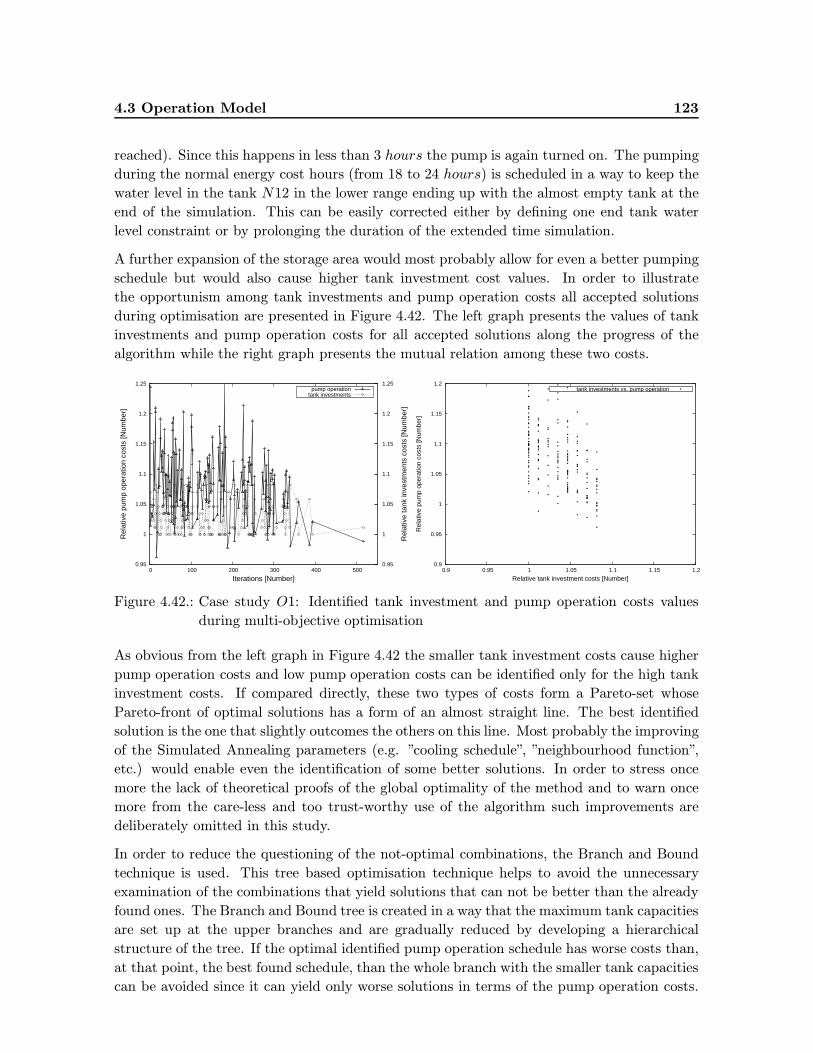
4.3 Operation Model 123
reached). Since this happens in less than 3 hours the pump is again turned on. The pumping
during the normal energy cost hours (from 18 to 24 hours) is scheduled in a way to keep the
water level in the tank N12 in the lower range ending up with the almost empty tank at the
end of the simulation. This can be easily corrected either by defining one end tank water
level constraint or by prolonging the duration of the extended time simulation.
A further expansion of the storage area would most probably allow for even a better pumping
schedule but would also cause higher tank investment cost values. In order to illustrate
the opportunism among tank investments and pump operation costs all accepted solutions
during optimisation are presented in Figure 4.42. The left graph presents the values of tank
investments and pump operation costs for all accepted solutions along the progress of the
algorithm while the right graph presents the mutual relation among these two costs.
0.95
1
1.05
1.1
1.15
1.2
1.25
0 100 200 300 400 500 0.95
1
1.05
1.1
1.15
1.2
1.25
Rel
ativ
e pu
mp
oper
atio
n co
sts
[Num
ber]
Rel
ativ
e ta
nk in
vest
men
ts c
osts
[Num
ber]
Iterations [Number]
pump operationtank investments
0.9
0.95
1
1.05
1.1
1.15
1.2
0.9 0.95 1 1.05 1.1 1.15 1.2
Rel
ativ
e pu
mp
oper
atio
n co
sts
[Num
ber]
Relative tank investment costs [Number]
tank investments vs. pump operation
Figure 4.42.: Case study O1: Identified tank investment and pump operation costs values
during multi-objective optimisation
As obvious from the left graph in Figure 4.42 the smaller tank investment costs cause higher
pump operation costs and low pump operation costs can be identified only for the high tank
investment costs. If compared directly, these two types of costs form a Pareto-set whose
Pareto-front of optimal solutions has a form of an almost straight line. The best identified
solution is the one that slightly outcomes the others on this line. Most probably the improving
of the Simulated Annealing parameters (e.g. ”cooling schedule”, ”neighbourhood function”,
etc.) would enable even the identification of some better solutions. In order to stress once
more the lack of theoretical proofs of the global optimality of the method and to warn once
more from the care-less and too trust-worthy use of the algorithm such improvements are
deliberately omitted in this study.
In order to reduce the questioning of the not-optimal combinations, the Branch and Bound
technique is used. This tree based optimisation technique helps to avoid the unnecessary
examination of the combinations that yield solutions that can not be better than the already
found ones. The Branch and Bound tree is created in a way that the maximum tank capacities
are set up at the upper branches and are gradually reduced by developing a hierarchical
structure of the tree. If the optimal identified pump operation schedule has worse costs than,
at that point, the best found schedule, than the whole branch with the smaller tank capacities
can be avoided since it can yield only worse solutions in terms of the pump operation costs.
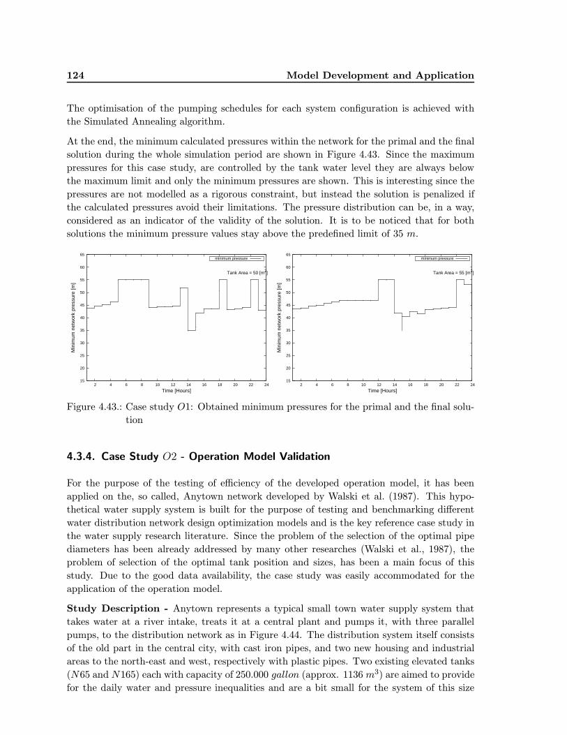
124 Model Development and Application
The optimisation of the pumping schedules for each system configuration is achieved with
the Simulated Annealing algorithm.
At the end, the minimum calculated pressures within the network for the primal and the final
solution during the whole simulation period are shown in Figure 4.43. Since the maximum
pressures for this case study, are controlled by the tank water level they are always below
the maximum limit and only the minimum pressures are shown. This is interesting since the
pressures are not modelled as a rigorous constraint, but instead the solution is penalized if
the calculated pressures avoid their limitations. The pressure distribution can be, in a way,
considered as an indicator of the validity of the solution. It is to be noticed that for both
solutions the minimum pressure values stay above the predefined limit of 35 m.
15
20
25
30
35
40
45
50
55
60
65
2 4 6 8 10 12 14 16 18 20 22 24
Min
imum
net
wor
k pr
essu
re [m
]
Time [Hours]
Tank Area = 50 [m2]
minimum pressure
15
20
25
30
35
40
45
50
55
60
65
2 4 6 8 10 12 14 16 18 20 22 24
Min
imum
net
wor
k pr
essu
re [m
]
Time [Hours]
Tank Area = 55 [m2]
minimum pressure
Figure 4.43.: Case study O1: Obtained minimum pressures for the primal and the final solu-
tion
4.3.4. Case Study O2 - Operation Model Validation
For the purpose of the testing of efficiency of the developed operation model, it has been
applied on the, so called, Anytown network developed by Walski et al. (1987). This hypo-
thetical water supply system is built for the purpose of testing and benchmarking different
water distribution network design optimization models and is the key reference case study in
the water supply research literature. Since the problem of the selection of the optimal pipe
diameters has been already addressed by many other researches (Walski et al., 1987), the
problem of selection of the optimal tank position and sizes, has been a main focus of this
study. Due to the good data availability, the case study was easily accommodated for the
application of the operation model.
Study Description - Anytown represents a typical small town water supply system that
takes water at a river intake, treats it at a central plant and pumps it, with three parallel
pumps, to the distribution network as in Figure 4.44. The distribution system itself consists
of the old part in the central city, with cast iron pipes, and two new housing and industrial
areas to the north-east and west, respectively with plastic pipes. Two existing elevated tanks
(N65 and N165) each with capacity of 250.000 gallon (approx. 1136 m3) are aimed to provide
for the daily water and pressure inequalities and are a bit small for the system of this size
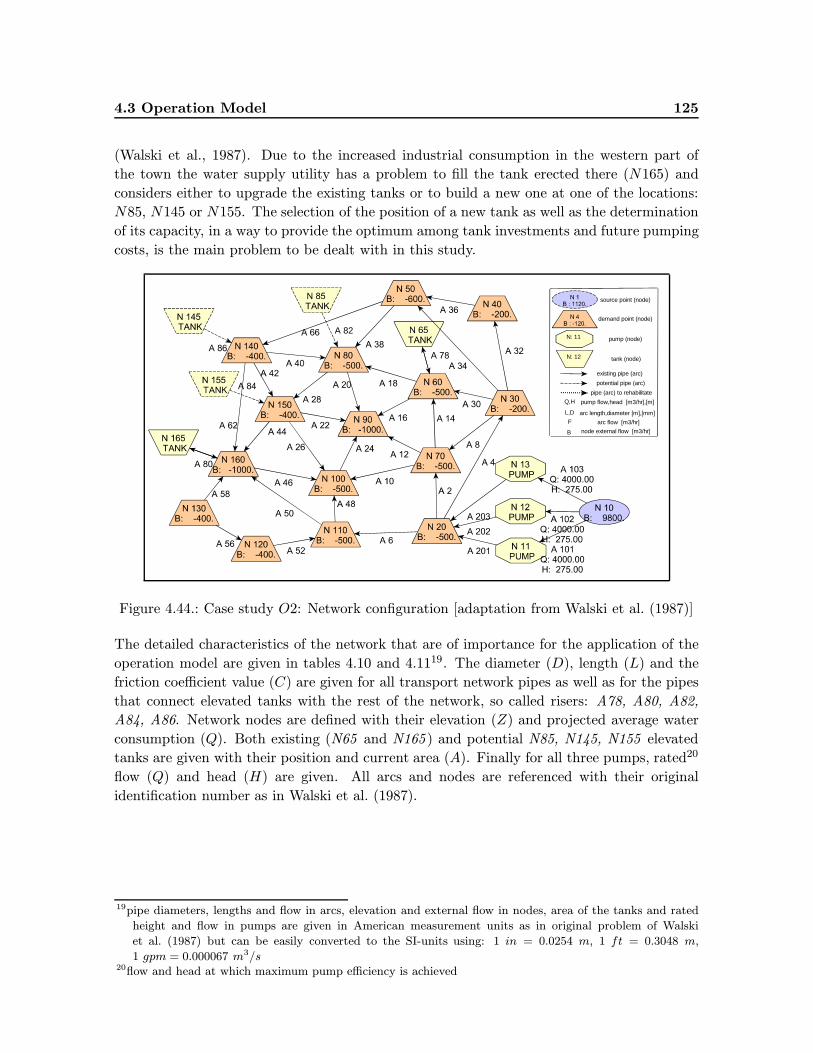
4.3 Operation Model 125
(Walski et al., 1987). Due to the increased industrial consumption in the western part of
the town the water supply utility has a problem to fill the tank erected there (N165) and
considers either to upgrade the existing tanks or to build a new one at one of the locations:
N85, N145 or N155. The selection of the position of a new tank as well as the determination
of its capacity, in a way to provide the optimum among tank investments and future pumping
costs, is the main problem to be dealt with in this study.
pump flow,head [m3/hr],[m]Q,H
pipe (arc) to rehabilitate
potential pipe (arc)
existing pipe (arc)
demand point (node)
pump (node)
source point (node)
N: 11
node external flow [m3/hr]B
arc flow [m3/hr]F
L,D arc length,diameter [m],[mm]
tank (node)N: 12
A 82
Figure 4.44.: Case study O2: Network configuration [adaptation from Walski et al. (1987)]
The detailed characteristics of the network that are of importance for the application of the
operation model are given in tables 4.10 and 4.1119. The diameter (D), length (L) and the
friction coefficient value (C) are given for all transport network pipes as well as for the pipes
that connect elevated tanks with the rest of the network, so called risers: A78, A80, A82,
A84, A86. Network nodes are defined with their elevation (Z) and projected average water
consumption (Q). Both existing (N65 and N165 ) and potential N85, N145, N155 elevated
tanks are given with their position and current area (A). Finally for all three pumps, rated20
flow (Q) and head (H) are given. All arcs and nodes are referenced with their original
identification number as in Walski et al. (1987).
19pipe diameters, lengths and flow in arcs, elevation and external flow in nodes, area of the tanks and rated
height and flow in pumps are given in American measurement units as in original problem of Walski
et al. (1987) but can be easily converted to the SI-units using: 1 in = 0.0254 m, 1 ft = 0.3048 m,
1 gpm = 0.000067 m3/s20flow and head at which maximum pump efficiency is achieved
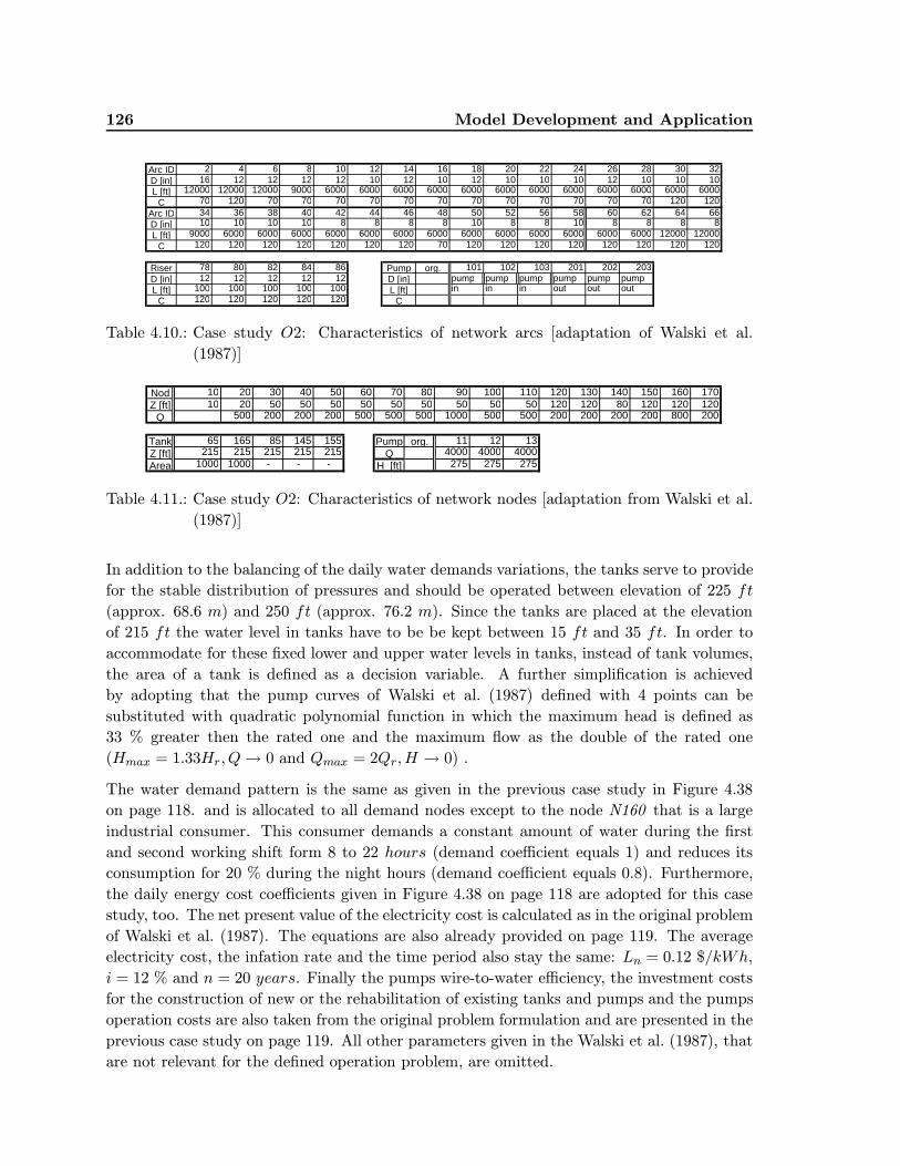
126 Model Development and Application
Arc ID 2 4 6 8 10 12 14 16 18 20 22 24 26 28 30 32D [in] 16 12 12 12 12 10 12 10 12 10 10 10 12 10 10 10L [ft] 12000 12000 12000 9000 6000 6000 6000 6000 6000 6000 6000 6000 6000 6000 6000 6000
C 70 120 70 70 70 70 70 70 70 70 70 70 70 70 120 120Arc ID 34 36 38 40 42 44 46 48 50 52 56 58 60 62 64 66D [in] 10 10 10 10 8 8 8 8 10 8 8 10 8 8 8 8L [ft] 9000 6000 6000 6000 6000 6000 6000 6000 6000 6000 6000 6000 6000 6000 12000 12000
C 120 120 120 120 120 120 120 70 120 120 120 120 120 120 120 120
Riser 78 80 82 84 86 Pump org. 101 102 103 201 202 203D [in] 12 12 12 12 12 D [in] pump pump pump pump pump pumpL [ft] 100 100 100 100 100 L [ft] in in in out out out
C 120 120 120 120 120 C
Table 4.10.: Case study O2: Characteristics of network arcs [adaptation of Walski et al.
(1987)]
Nod 10 20 30 40 50 60 70 80 90 100 110 120 130 140 150 160 170Z [ft] 10 20 50 50 50 50 50 50 50 50 50 120 120 80 120 120 120
Q 500 200 200 200 500 500 500 1000 500 500 200 200 200 200 800 200
Tank 65 165 85 145 155 Pump org. 11 12 13Z [ft] 215 215 215 215 215 Q 4000 4000 4000Area 1000 1000 - - - H [ft] 275 275 275
Table 4.11.: Case study O2: Characteristics of network nodes [adaptation from Walski et al.
(1987)]
In addition to the balancing of the daily water demands variations, the tanks serve to provide
for the stable distribution of pressures and should be operated between elevation of 225 ft
(approx. 68.6 m) and 250 ft (approx. 76.2 m). Since the tanks are placed at the elevation
of 215 ft the water level in tanks have to be be kept between 15 ft and 35 ft. In order to
accommodate for these fixed lower and upper water levels in tanks, instead of tank volumes,
the area of a tank is defined as a decision variable. A further simplification is achieved
by adopting that the pump curves of Walski et al. (1987) defined with 4 points can be
substituted with quadratic polynomial function in which the maximum head is defined as
33 % greater then the rated one and the maximum flow as the double of the rated one
(Hmax = 1.33Hr, Q → 0 and Qmax = 2Qr,H → 0) .
The water demand pattern is the same as given in the previous case study in Figure 4.38
on page 118. and is allocated to all demand nodes except to the node N160 that is a large
industrial consumer. This consumer demands a constant amount of water during the first
and second working shift form 8 to 22 hours (demand coefficient equals 1) and reduces its
consumption for 20 % during the night hours (demand coefficient equals 0.8). Furthermore,
the daily energy cost coefficients given in Figure 4.38 on page 118 are adopted for this case
study, too. The net present value of the electricity cost is calculated as in the original problem
of Walski et al. (1987). The equations are also already provided on page 119. The average
electricity cost, the infation rate and the time period also stay the same: Ln = 0.12 $/kWh,
i = 12 % and n = 20 years. Finally the pumps wire-to-water efficiency, the investment costs
for the construction of new or the rehabilitation of existing tanks and pumps and the pumps
operation costs are also taken from the original problem formulation and are presented in the
previous case study on page 119. All other parameters given in the Walski et al. (1987), that
are not relevant for the defined operation problem, are omitted.
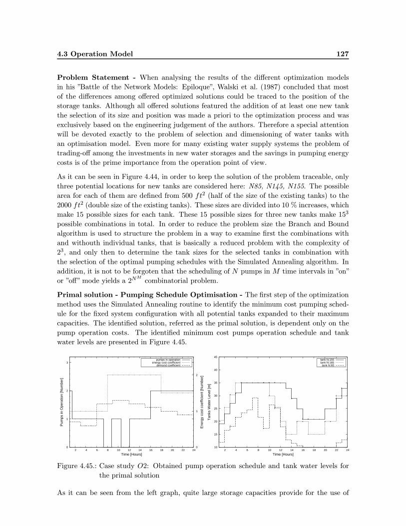
4.3 Operation Model 127
Problem Statement - When analysing the results of the different optimization models
in his ”Battle of the Network Models: Epiloque”, Walski et al. (1987) concluded that most
of the differences among offered optimized solutions could be traced to the position of the
storage tanks. Although all offered solutions featured the addition of at least one new tank
the selection of its size and position was made a priori to the optimization process and was
exclusively based on the engineering judgement of the authors. Therefore a special attention
will be devoted exactly to the problem of selection and dimensioning of water tanks with
an optimisation model. Even more for many existing water supply systems the problem of
trading-off among the investments in new water storages and the savings in pumping energy
costs is of the prime importance from the operation point of view.
As it can be seen in Figure 4.44, in order to keep the solution of the problem traceable, only
three potential locations for new tanks are considered here: N85, N145, N155. The possible
area for each of them are defined from 500 ft2 (half of the size of the existing tanks) to the
2000 ft2 (double size of the existing tanks). These sizes are divided into 10 % increases, which
make 15 possible sizes for each tank. These 15 possible sizes for three new tanks make 153
possible combinations in total. In order to reduce the problem size the Branch and Bound
algorithm is used to structure the problem in a way to examine first the combinations with
and withouth individual tanks, that is basically a reduced problem with the complexity of
23, and only then to determine the tank sizes for the selected tanks in combination with
the selection of the optimal pumping schedules with the Simulated Annealing algorithm. In
addition, it is not to be forgoten that the scheduling of N pumps in M time intervals in ”on”
or ”off” mode yields a 2NM
combinatorial problem.
Primal solution - Pumping Schedule Optimisation - The first step of the optimization
method uses the Simulated Annealing routine to identify the minimum cost pumping sched-
ule for the fixed system configuration with all potential tanks expanded to their maximum
capacities. The identified solution, referred as the primal solution, is dependent only on the
pump operation costs. The identified minimum cost pumps operation schedule and tank
water levels are presented in Figure 4.45.
0
1
2
3
2 4 6 8 10 12 14 16 18 20 22 24 0
1
2
Pum
ps in
Ope
ratio
n [N
umbe
r]
Ene
rgy
cost
coe
ffici
ent [
Num
ber]
Time [Hours]
pumps in operationenergy cost coefficient
demand coefficient
10
15
20
25
30
35
40
45
2 4 6 8 10 12 14 16 18 20 22 24
Tan
ks W
ater
Lev
el [m
]
Time [Hours]
tank N:155tank N:165
tank N:65
Figure 4.45.: Case study O2: Obtained pump operation schedule and tank water levels for
the primal solution
As it can be seen from the left graph, quite large storage capacities provide for the use of
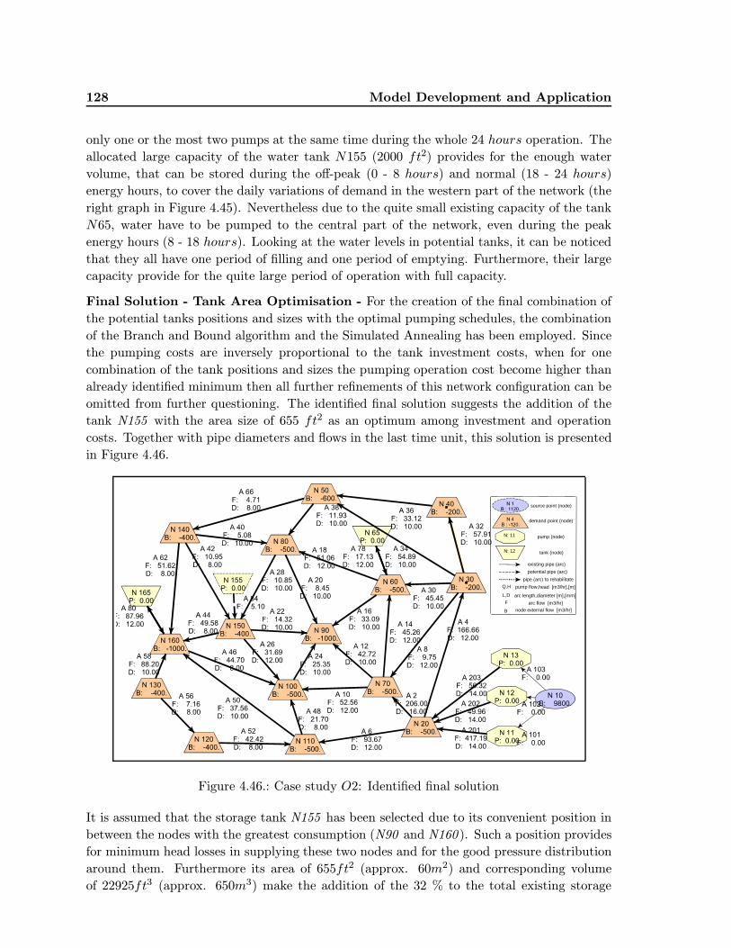
128 Model Development and Application
only one or the most two pumps at the same time during the whole 24 hours operation. The
allocated large capacity of the water tank N155 (2000 ft2) provides for the enough water
volume, that can be stored during the off-peak (0 - 8 hours) and normal (18 - 24 hours)
energy hours, to cover the daily variations of demand in the western part of the network (the
right graph in Figure 4.45). Nevertheless due to the quite small existing capacity of the tank
N65, water have to be pumped to the central part of the network, even during the peak
energy hours (8 - 18 hours). Looking at the water levels in potential tanks, it can be noticed
that they all have one period of filling and one period of emptying. Furthermore, their large
capacity provide for the quite large period of operation with full capacity.
Final Solution - Tank Area Optimisation - For the creation of the final combination of
the potential tanks positions and sizes with the optimal pumping schedules, the combination
of the Branch and Bound algorithm and the Simulated Annealing has been employed. Since
the pumping costs are inversely proportional to the tank investment costs, when for one
combination of the tank positions and sizes the pumping operation cost become higher than
already identified minimum then all further refinements of this network configuration can be
omitted from further questioning. The identified final solution suggests the addition of the
tank N155 with the area size of 655 ft2 as an optimum among investment and operation
costs. Together with pipe diameters and flows in the last time unit, this solution is presented
in Figure 4.46.
pump flow,head [m3/hr],[m]Q,H
pipe (arc) to rehabilitate
potential pipe (arc)
existing pipe (arc)
demand point (node)
pump (node)
source point (node)
N: 11
node external flow [m3/hr]B
arc flow [m3/hr]F
L,D arc length,diameter [m],[mm]
tank (node)N: 12
Figure 4.46.: Case study O2: Identified final solution
It is assumed that the storage tank N155 has been selected due to its convenient position in
between the nodes with the greatest consumption (N90 and N160 ). Such a position provides
for minimum head losses in supplying these two nodes and for the good pressure distribution
around them. Furthermore its area of 655ft2 (approx. 60m2) and corresponding volume
of 22925ft3 (approx. 650m3) make the addition of the 32 % to the total existing storage
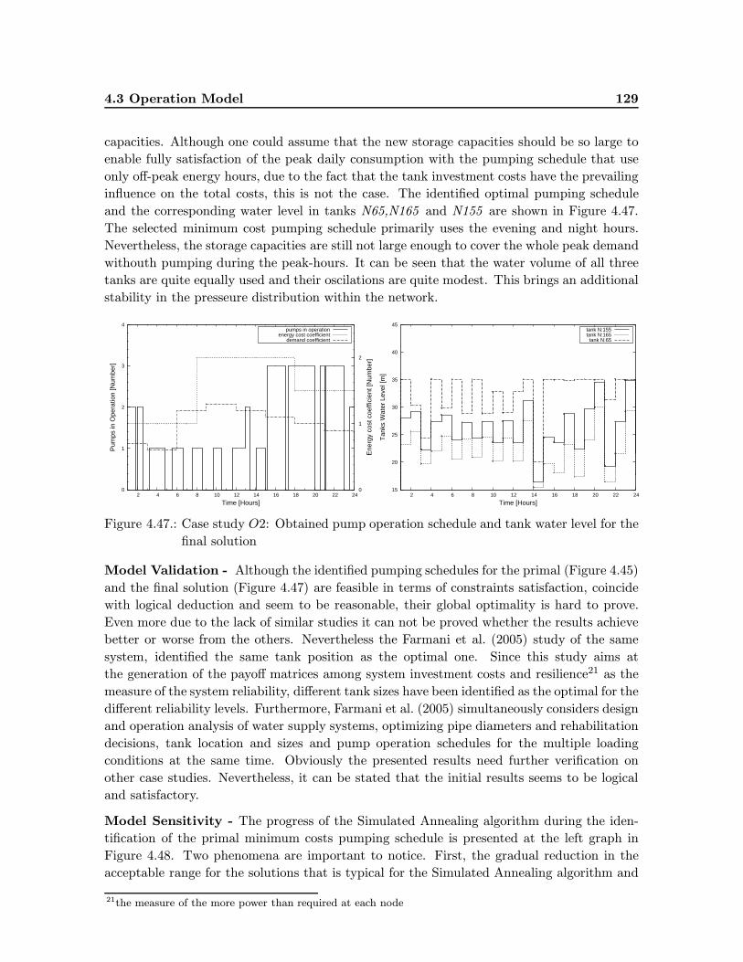
4.3 Operation Model 129
capacities. Although one could assume that the new storage capacities should be so large to
enable fully satisfaction of the peak daily consumption with the pumping schedule that use
only off-peak energy hours, due to the fact that the tank investment costs have the prevailing
influence on the total costs, this is not the case. The identified optimal pumping schedule
and the corresponding water level in tanks N65,N165 and N155 are shown in Figure 4.47.
The selected minimum cost pumping schedule primarily uses the evening and night hours.
Nevertheless, the storage capacities are still not large enough to cover the whole peak demand
withouth pumping during the peak-hours. It can be seen that the water volume of all three
tanks are quite equally used and their oscilations are quite modest. This brings an additional
stability in the presseure distribution within the network.
0
1
2
3
4
2 4 6 8 10 12 14 16 18 20 22 24 0
1
2
Pum
ps in
Ope
ratio
n [N
umbe
r]
Ene
rgy
cost
coe
ffici
ent [
Num
ber]
Time [Hours]
pumps in operationenergy cost coefficient
demand coefficient
15
20
25
30
35
40
45
2 4 6 8 10 12 14 16 18 20 22 24
Tan
ks W
ater
Lev
el [m
]
Time [Hours]
tank N:155tank N:165
tank N:65
Figure 4.47.: Case study O2: Obtained pump operation schedule and tank water level for the
final solution
Model Validation - Although the identified pumping schedules for the primal (Figure 4.45)
and the final solution (Figure 4.47) are feasible in terms of constraints satisfaction, coincide
with logical deduction and seem to be reasonable, their global optimality is hard to prove.
Even more due to the lack of similar studies it can not be proved whether the results achieve
better or worse from the others. Nevertheless the Farmani et al. (2005) study of the same
system, identified the same tank position as the optimal one. Since this study aims at
the generation of the payoff matrices among system investment costs and resilience21 as the
measure of the system reliability, different tank sizes have been identified as the optimal for the
different reliability levels. Furthermore, Farmani et al. (2005) simultaneously considers design
and operation analysis of water supply systems, optimizing pipe diameters and rehabilitation
decisions, tank location and sizes and pump operation schedules for the multiple loading
conditions at the same time. Obviously the presented results need further verification on
other case studies. Nevertheless, it can be stated that the initial results seems to be logical
and satisfactory.
Model Sensitivity - The progress of the Simulated Annealing algorithm during the iden-
tification of the primal minimum costs pumping schedule is presented at the left graph in
Figure 4.48. Two phenomena are important to notice. First, the gradual reduction in the
acceptable range for the solutions that is typical for the Simulated Annealing algorithm and
21the measure of the more power than required at each node
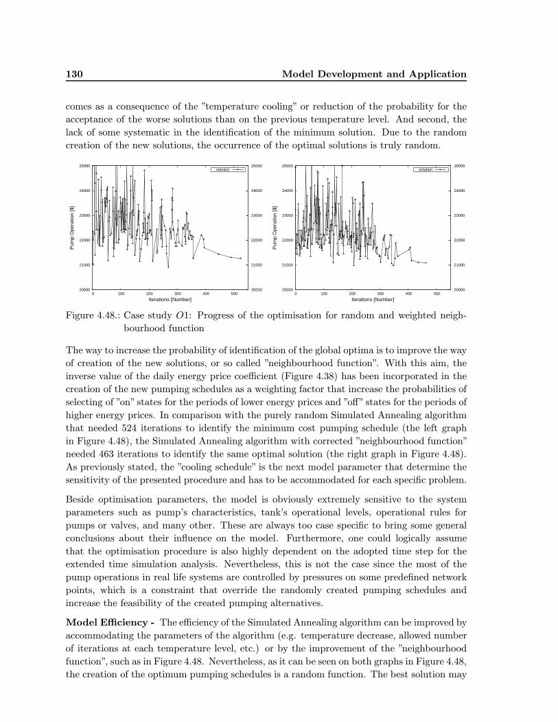
130 Model Development and Application
comes as a consequence of the ”temperature cooling” or reduction of the probability for the
acceptance of the worse solutions than on the previous temperature level. And second, the
lack of some systematic in the identification of the minimum solution. Due to the random
creation of the new solutions, the occurrence of the optimal solutions is truly random.
20000
21000
22000
23000
24000
25000
0 100 200 300 400 500 20000
21000
22000
23000
24000
25000
Pum
p O
pera
tion
[$]
Iterations [Number]
solution
20000
21000
22000
23000
24000
25000
0 100 200 300 400 500 20000
21000
22000
23000
24000
25000
Pum
p O
pera
tion
[$]
Iterations [Number]
solution
Figure 4.48.: Case study O1: Progress of the optimisation for random and weighted neigh-
bourhood function
The way to increase the probability of identification of the global optima is to improve the way
of creation of the new solutions, or so called ”neighbourhood function”. With this aim, the
inverse value of the daily energy price coefficient (Figure 4.38) has been incorporated in the
creation of the new pumping schedules as a weighting factor that increase the probabilities of
selecting of ”on” states for the periods of lower energy prices and ”off” states for the periods of
higher energy prices. In comparison with the purely random Simulated Annealing algorithm
that needed 524 iterations to identify the minimum cost pumping schedule (the left graph
in Figure 4.48), the Simulated Annealing algorithm with corrected ”neighbourhood function”
needed 463 iterations to identify the same optimal solution (the right graph in Figure 4.48).
As previously stated, the ”cooling schedule” is the next model parameter that determine the
sensitivity of the presented procedure and has to be accommodated for each specific problem.
Beside optimisation parameters, the model is obviously extremely sensitive to the system
parameters such as pump’s characteristics, tank’s operational levels, operational rules for
pumps or valves, and many other. These are always too case specific to bring some general
conclusions about their influence on the model. Furthermore, one could logically assume
that the optimisation procedure is also highly dependent on the adopted time step for the
extended time simulation analysis. Nevertheless, this is not the case since the most of the
pump operations in real life systems are controlled by pressures on some predefined network
points, which is a constraint that override the randomly created pumping schedules and
increase the feasibility of the created pumping alternatives.
Model Efficiency - The efficiency of the Simulated Annealing algorithm can be improved by
accommodating the parameters of the algorithm (e.g. temperature decrease, allowed number
of iterations at each temperature level, etc.) or by the improvement of the ”neighbourhood
function”, such as in Figure 4.48. Nevertheless, as it can be seen on both graphs in Figure 4.48,
the creation of the optimum pumping schedules is a random function. The best solution may
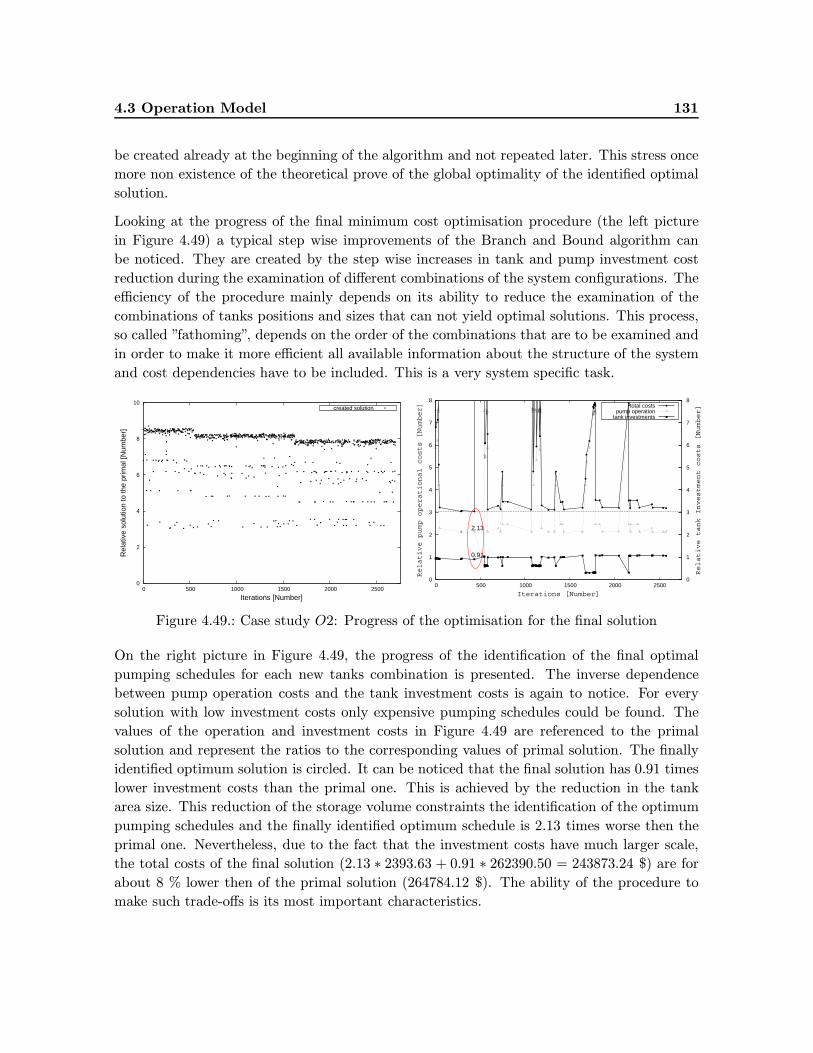
4.3 Operation Model 131
be created already at the beginning of the algorithm and not repeated later. This stress once
more non existence of the theoretical prove of the global optimality of the identified optimal
solution.
Looking at the progress of the final minimum cost optimisation procedure (the left picture
in Figure 4.49) a typical step wise improvements of the Branch and Bound algorithm can
be noticed. They are created by the step wise increases in tank and pump investment cost
reduction during the examination of different combinations of the system configurations. The
efficiency of the procedure mainly depends on its ability to reduce the examination of the
combinations of tanks positions and sizes that can not yield optimal solutions. This process,
so called ”fathoming”, depends on the order of the combinations that are to be examined and
in order to make it more efficient all available information about the structure of the system
and cost dependencies have to be included. This is a very system specific task.
0
2
4
6
8
10
0 500 1000 1500 2000 2500
Rel
ativ
e so
lutio
n to
the
prim
al [N
umbe
r]
Iterations [Number]
created solution
0
1
2
3
4
5
6
7
8
0 500 1000 1500 2000 2500 0
1
2
3
4
5
6
7
8
Relative pump operational costs [Number]
Relative tank Investment costs [Number]
Iterations [Number]
2.13
0.91
total costspump operation
tank investments
Figure 4.49.: Case study O2: Progress of the optimisation for the final solution
On the right picture in Figure 4.49, the progress of the identification of the final optimal
pumping schedules for each new tanks combination is presented. The inverse dependence
between pump operation costs and the tank investment costs is again to notice. For every
solution with low investment costs only expensive pumping schedules could be found. The
values of the operation and investment costs in Figure 4.49 are referenced to the primal
solution and represent the ratios to the corresponding values of primal solution. The finally
identified optimum solution is circled. It can be noticed that the final solution has 0.91 times
lower investment costs than the primal one. This is achieved by the reduction in the tank
area size. This reduction of the storage volume constraints the identification of the optimum
pumping schedules and the finally identified optimum schedule is 2.13 times worse then the
primal one. Nevertheless, due to the fact that the investment costs have much larger scale,
the total costs of the final solution (2.13 ∗ 2393.63 + 0.91 ∗ 262390.50 = 243873.24 $) are for
about 8 % lower then of the primal solution (264784.12 $). The ability of the procedure to
make such trade-offs is its most important characteristics.
5. Conclusions and Outlook
Keeping in mind that the main objective of this study was to develop a modelling methodology
for multi-objective analysis and optimisation of planning, design and operation of water supply
systems, the suggested methodological concepts just as well as their implementations in the
three computer models are discussed in this chapter. The main advantages and some of
identified disadvantages with respect to the achievement of the stated research objectives are
summarized. Based on this, some needed further improvements and possible new research
activities are given.
5.1. Methodology Development
An attempt to further approach the integrative consideration of natural environment and
human built-in water supply systems has been made by developing the methodology that aims
at the multi-objective and risk-based decision support in planning, design and operation of
water supply systems. In order to develop an systematic, integrative, transparent, and above
all easily applicable methodology, the following issues have been treated:
Joint analysis of technical, environmental, economic and social aspects of water
supply systems - When developing a new or analysing an existing water supply system it is
of crucial importance to encompass all different positive and negative impacts it may has on
a wide range of environmental, economic or social values. In order to enable the integrative
consideration of impacts that have different units, times and scales, they are approximated
with single-variable functions of some system parameter such as flow, capacity, water with-
drawal etc.. Although such simplified impacts quantification adds to the uncertainty of the
methodology, its has been argued that: a) the integration of various impacts is of much
greater importance that a more accurate analysis of only one, b) the accuracy of the impact
functions may be accommodated to the purpose of an analysis and available time, money
and other resources, and c) the here introduced uncertainty has a same order of magnitude
as most other input parameters of the analysis such as predicted water demands, interest
rates, hydraulic characteristics, etc.. Furthermore, the methodology has been accommodated
to cover a broad range of possible impact relations and to deal with various possible forms of
impact functions (i.e linear, convex, concave and step-wise). In comparison with already ex-
isting methodologies for the optimisation of water supply systems this represents a significant
improvement.
Integration of interests and objectives of different stakeholders and decision mak-
ers already in the formulation of alternative solutions - Since the creation and eval-
uation of a project or set of actions is highly dependent on preferences (utilities) of decision
5.1 Methodology Development 133
makers toward individual objectives or criteria, these preferences are included in the sys-
tems’ analysis. The developed methodology adopts the Multiple Criteria Decision Analysis
approach in which the selection of the optimal solution is done by a trade-off among differ-
ent identified optimal solutions that correspond to different combinations of decision makers’
preferences. It has been stated that the incorporation of the preferences already in the for-
mulation of alternative solutions: a) significantly influences the direction of the optimisation
search and improve efficiency of the optimisation algorithm, b) advance the development
of the alternatives that are better suited to the decision makers’ preferences increasing the
chances for the selection of these solutions, and c) enable ease identification of the broad
range of alternative options simply by changing the preferences (weights) toward different
objectives. If known that in most decision support systems first develop optimal alternatives
and then evaluate them according to the preferences of the decision makers, the advantages
of the integration of decision makers’s preferences already in the alternatives’ development
phase are more then obvious.
Handling of very complex problems with simple enough and easily understand-
able methods - Just as well as it is important to develop a methodology that is able to
encompass the very sophisticated structure and function of water supply systems and the
complex, multi-objective and multi-preference nature of water supply management problems,
it is equally important that developed methodology stays simple and understandable enough
to be applicable by water supply practitioners. In order to provide for an understandable
representation of the water supply systems structure, the Network Concept from the Graph
Theory has been used. The Minimum Cost Flow Network optimisation problem that is ac-
commodated to handle multiple criteria and fixed and variable impacts at the same time,
has been used to formulate the objectives of the analysis. Finally, a very robust optimisation
technique (i.e. the Simulated Annealing) has been used to solve this non-linear and non-
convex optimisation problem defined on conforming flow paths. The dependence of network
flow from other network characteristics allowed for the ease application of the same pro-
blem formulation in the optimisation of different parameters such as system layout, sources’
withdrawals, pipe diameters, tank capacities, pump schedules, etc.. In order to improve the
ability of the procedure to deal with discrete problem and create and question a wide range
of possible system configurations, the Simulated Annealing is embedded within the Branch
and Bound procedure. The combination of these techniques applied on network problems,
attained very similar results and proved to be slightly more efficient than most of the other
often used heuristic techniques such as Genetic Algorithm.
Incorporation of robustness, flexibility and reliability considerations in the ma-
nagement of water supply systems - Robust, flexible and reliable planning, design and
operation of water supply systems are new focus areas of the modern management of water
supply systems. In addition to the implicit consideration of the systems robustness and flexi-
bility by incorporation of multiple objectives and criteria in the development of management
alternatives, the reliability issue has been explicitly addressed. The methodology has been
accommodated to deal with the component failure analysis. An advanced method for the
addition of spare capacities to the network systems (i.e. the Path Restoration method of
Iraschko et al. 1998; Iraschko and Grover 2000) has been applied to identify the least cost
system configuration that can provide for the functioning of a system in a case of failure
134 Conclusions and Outlook
of some component. The same method can be used to address any other deterministically
defined stress condition, providing for a powerful optimisation tool especially useful in the
design analysis of water supply systems.
Incorporation of uncertainty considerations, users’ expectations and their risk
tolerance into the evaluation of alternative management options - In addition to
the deterministically defined stress conditions, the consideration of uncertainty and variability
issues is just as equally important for flexible and reliable water supply systems planning,
design and operation. An advanced sampling based technique (i.e. the Latin Hypercube
Sampling of Iman and Shortencarier 1984) has been employed to efficiently create samples of
uncertain or variable parameters that have some predefined probabilistic characteristic and
can be used for the testing of the systems performance and the calculation of their reliability
in terms of the probability of non-failure. The evaluation of the calculated reliability then is
subjective to the users’ expectations from the systems or the decision makers’ risk perception
toward some system failure. The incorporation of these two aspects in the methodology aligns
with new engineering trends toward the substitution of fixed engineering standards and codes
of practice with more risk-oriented approaches for management of water supply systems.
Transparent and easily applicable decision support for the integrative manage-
ment of water supply systems - Finally, the transparency of the methodology is one
of the basic prerequisites for its acceptance in praxis. An effort has been made to provide
for the complete transparency of the methodology starting from the definition of objectives,
adoption of criteria and selection of decision variables, through the approximation of impact
functions, control of the optimisation procedure and creation of Pareto-optimal alternatives
to the integration of decision makers’ preference, their risk perception and evaluation of the
parameters’ uncertainty and reliability of water supply systems. This has been seen as a
good way to promote greater involvement and participation of the decision makers since they
are not just involved in the selection of some predefined alternatives but the alternatives are
accommodated to their perception of the needed system performance and reliability. Fur-
thermore, the multi-objectivity and risk-orientation of the analysis enable for the risk prone
decision makers to sacrifice on some objectives (e.g. system performances in terms of deliv-
ered pressures) in order to achieve better on some another (e.g. savings in costs). This should
add to the identification of sustainable development options that may improve the long term
management of water supply systems.
5.2. Models Development
In order to enable easier use and application of the developed methodology, three computer
model have been developed. Since the main aim and the purpose of the analysis differ for
each management stage, the general methodological concepts have been accommodated to
address the specific issues of planning, design and operation of water supply systems and
have been implemented into corresponding models.
Planning Model - The fundamental questions of water supply planning studies such as
the selection of the natural resources for human use, determination of the extent of water
5.2 Models Development 135
extraction and the identification of the most optimal water distribution can be addressed
with the developed planning model. Furthermore, the multi-objective and multi-preference
problem formulation provides for the identification of a wide range of solutions that are
optimal for different combinations of preferences toward individual objectives. For example
the single-objective solutions serve for the identification of the effects of the advancement
of only economic, environmental or social criteria. In contrast, the multi-objective solutions
offer a wide range of Pareto-optimal alternatives for the negotiation and trade-off among
decision makers in order to identify the best compromise solution. It has been proved that
the model is: a) able to deal with multiple objectives and criteria in a systematic way, b) able
to encompass multiple preferences toward different objectives and to identifying a full range of
valid solutions and c) has slightly better efficiency then some other approximation algorithms
due to the more precise representation of the systems. Nevertheless, the main deficiencies of
the model are: a) a very simplified representation of the effects and consequence of the systems
with the impact functions and b) non-existence of the theoretical proof for the optimality of
the identified solutions.
Design Model - The multi-objectivity of the water supply design problem reflects not so
much in the integration of different systems impacts, but much more in the need to integrate
different categories of importance into one analysis. Beside technical and economic issues, the
incorporation of uncertainty, risk and reliability plays a prevailing role for the determination of
optimal systems sizes and capacities. Therefore the design analysis is composed of two steps.
The design model first identifies the minimum cost system configuration that satisfies all given
constraints. The validity of this single-objective solution has been proved on two theoretical
case studies. Furthermore, the model showed a very good efficiency in comparison with some
other very often used approaches such as Genetic Algorithm. Then, the performance of
the systems is assessed by implementing the component failure analysis and the parameters’
uncertainty analysis. The combination of these two provided for the easily manageable and
clearly understandable assessment of the systems reliability in terms of the probability of
not-failure. The decision makers’ risk acceptance level present the basis for the selection of
the optimal design option by trading-off between the system’s costs and its reliability. It has
been proved that the model is able to: a) deal with complex, discrete, NP-hard problem of
the selection of the minimum cost water supply network configuration, b) identify just as
good and valid solutions as the other models reported in the literature with approximately
the same or even better efficiency of the algorithm, c) address the reliability issue with the
combination of the deterministically defined component failure analysis and the stochastically
based performance failure analysis for some uncertain or variable parameters and d) allow for
the risk-based selection among system performances and reliability on one side and economic
costs on the other. Some important limitations of the model are: a) simplified consideration
of the pressure distribution within the optimisation model, b) backward going approach
for the assessment of the system reliability and addition of an external network solver for
more precise calculation of the system performances, and c) simplified characterisation of the
mutual dependencies of the uncertain and variable parameters in form of correlation matrices.
Operation Model - The identification of possible trade-off between investment costs in
water storage facilities and operation costs of water pumping stations is adopted as the main
problem to deal with. Although both mentioned objectives are expressed in the same terms,
136 Conclusions and Outlook
the addition of time dimension to the optimisation problem significantly adds upon its com-
plexity. Furthermore instead of water flow as the one main decision variable like in the
planning and the design problem, the tanks sizes and pumping schedules now represent two
distinct decision variables. Both variables are discrete and the pumping schedules have an
additional dimension since they are distributed in time. The addition of the time dimension
significantly adds up on the model complexity since the flow vector is not any more a station-
ary value but instead the set of, in time ordered, flow vectors. Furthermore, a network solver
of Gessler et al. (1985) had to be coupled with the optimisation model for the calculation of
network flows, pressures and tank levels during the extended period simulation. Nevertheless,
the model managed to identify reasonable pumping schedules and tank configurations for the
two applied case studies. Unfortunately the exact validity of the results could not be proved
due to the lack of similar studies. It has been stated that the model: a) has a possibility
to model various components such as pressure reducing valves, check valve, booster stations,
etc. and different sort of operation rules, and b) is able to deal with a complex problem of
simultaneous selection of the minimum cost tanks positions and sizes and the identification
of the optimal pumping schedules. Still the main limitations for its application in operation
of water supply systems are the facts that: a) it focuses only on the trade-off among tank
investment and pump operation costs and b) the optimality of the produced solutions can
not be theoretically proved.
5.3. Outlook
From the presented study it can be concluded that the use of the network concept provides a
very good conceptual representation and increases the number of additional information that
can be assessed in structural or capacity analysis of water supply systems. Furthermore, it
improved the efficiency of the optimisation algorithms and added to the applicability of the
developed methodology. As far as the integration of various objectives into one modelling en-
vironment is concerned, the disadvantages and difficulties in the development and validation
of the impact functions have been recognized. Nevertheless such an approach enable integra-
tive analysis of different economic, environmental and social issues and is adopted as accurate
enough. The implementation of the decision makers’ preferences in the development of the
optimal alternatives has been recognised here as more important. In addition, the evaluation
and selection of the optimal alternatives has been accommodated to the risk perception of
the decision makers in order to provide for their greater participation and development of
sustainable development options. Finally, the suggested methods for dealing with uncertainty
and reliability issues are deliberately chosen to be as simple as possible in order to enable for
their ease accommodation in different water supply analyses. Nevertheless, they provide for
systematic and transparent incorporation of these issues in planing,design and operation of
water supply systems.
Based on the results of the models implementation, it can be stated that the developed
methodology provides for the achievement of the stated objectives. Nevertheless, the more
detailed testing and validation of the models is necessary. Application of the models on some
real-life cases would be especially beneficial as well as the confrontation of the produced

5.3 Outlook 137
results with the expert’s knowledge from the field. Furthermore, although based on the same
methodology the individual models are still functioning completely isolated. An integration
of the developed planning, design and operation model into one decision support system
for water supply systems management would not only improve the data exchange among
models, but also significantly add upon their usefulness and user-friendliness. In addition,
many additional options (such as new objectives and decision variables) could be included
in the models and especially in the operation model. Similarly, the rehabilitation stage of
the water supply management could be developed on the same methodological concepts but
as a separate model. Finally the applied methods can be exchanged with some others just
as long as this improve the efficiency, applicability or transparency of the methodology. The
selection of the individual methods for the solution of the network problem, multi-objective
optimisation, or uncertainty, risk and reliability assessment is quite irrelevant in comparison
to the importance of integration of these issues in one analysis.


Bibliography
Abebe, A. & Solomatine, D. (1998). Application of global optimization to the design of pipe
networks. In: 3rd International Conferences on Hydroinformatics-98, pages 989–996, A.A.
Balkema Publishers. Copenhagen, Denmark.
Adelman, L. (1992). Evaluating Decision Support and Expert Systems. John Wiley and Sons
Inc., New York, Chichester, Brisbane, Toronto.
Ahuja, R., Magnanti, T., & Orlin, J. (1993). Network Flows: Theory, Algorithms, and
Applications. Prentice-Hall Inc., Englewood Cliffs, New Jersey.
Allenby, B. (2004). Infrastructure in the anthropocene: Example of information and commu-
nication technology. Journal of Infrastructure Systems, 10(3):79–86.
Alperovits, E. & Shamir, U. (1977). Design of optimal water distribution systems. Water
Resources Research, 13(6):885–900.
Ang, A.-S. & Tang, W. (1984). Probability Concepts in Engineering Planning and Desing,
Vol. 2. John Willey and Sons, New York.
AWRA (2001). Decision Support Systems for Water Resources Management. American Water
Resources Association, Snowbird, Utah.
Awumah, K., Goulter, I., & Bhatt, S. (1990). Assessment of reliability in water distribution
networks using entropy based measures. Stochastic Hydrology and Hydraulics, 4:309–320.
Awumah, K., Goulter, I., & Bhatt, S. (1991). Entropy-based redundancy measures in water-
distribution networks. Journal of Hydraulic Engineering, 117(5):595–614.
Awumah, K., Goulter, I., & Bhatt, S. (1992). Maximizing entropy defined reliability of water
distribution networks. Engineering Optimization, 20(1):57–80.
Babayan, A., Kapelan, Z., Savic, D., & Walters, G. (2003). Least cost design of water distri-
bution networks under demand uncertainty. In: Advances in Water Supply Management,
Proceedings of the International Conference on Computing and Control for the Water In-
dustry, A.A. Balkema Publishers. 15-17. September. London, UK.
Babayan, A., Savic, D., & Walters, G. (2004). Multiobjective optimization of water dis-
tribution systems under uncertain demand and pipe roughness. In: IFAC Workshop on
Modelling and Control for Participatory Planning and Managing Water Systems, Interna-
tional Federation of Automatic Control. September. Venice, Italy.
Bao, Y. & Mays, L. (1990). Model for water distribution system reliability. Journal of
Hydraulic Engineering, 116(9):1119–1137.
Baran, B., Von Lucken, C., & Sotelo, A. (2005). Multi-objective pump scheduling optimisa-
tion using evolutionary strategies. Advances in Engineering Software, 36(1):39–48.
Bardossy, A., Bogardi, I., & Duckstein, L. (1983). Multiple criteria decision making using
fuzzy objectives: A case study. In: 6. European Congress on Operations Research, Springer
Verlag. 19. - 22. Juli. Vienna, Austria.
Bardossy, A. & Duckstein, L. (1995). Fuzzy Rule-Based Modelling with Applications to Geo-
physical, Biological and Engineering Systems. CRC Press Inc., Boca Raton.
Beder, S. (2002). Economy and environment: Competitors or part-
ners. Pacific Ecologist, 3:50–56. Retrieved January 15, 2006, from
http://www.uow.edu.au/arts/sts/sbeder/pacific2.html.
Beecher, J. A., Higbee, J., Manzel, A., & Dooley, R. (1996). The regionalization of water
utilities: Perspectives, literature review and annotated bibliography. Report 96-21, The
National Regulatory Research Institute, The Ohio State University, Ohio.
Beim, G. & Hobbs, B. (1988). Analytical simulation of water system capacity reliability. 2:
Markov chain approach and verification of models. Water Resources Research, 24(9):1445–
1458.
Belaineh, G., Peralta, R., & Hughes, T. (1999). Simulation/optimization modeling for
water resources management. Journal of Water Resources Planning and Management,
125(3):154–161.
Bertsekas, D. (1998). Network Optimization: Continuous and Discrete. Athena Scientific
Belmont, Mass., Massachusetts.
Bhave, P. (1978). Noncomputer optimization of single-source networks. Journal of the Envi-
ronmental Engineering Division, 104(4):799–813.
Bhave, P. & Gupta, R. (2004). Optimal design of water distribution networks for fuzzy
demands. Civil Engineering and Environmental Systems, 21(4):229–245.
Biggs, N., Lloyd, E., & Wilson, R. (1976). Graph Theory 1739-1936. Clarendon Prss, Oxford.
Biswas, A. (1996). Water Resources, Environmental Planning, Management and Develop-
ment. McGraw-Hill, New York.
Bogardi, I., Duckstein, L., & Bardossy, A. (1987). A fuzzy reliability model of water supply
during droughts. In: Fall National Meeting of the AGU, American Geophysical Union.
November. San Francisco, USA.
Bogardi, J. & Kundzewicz, Z. (2002). Risk, Reliability, Uncertainty and Robustness of Water
Resource Systems. International Hydrology Series, Cambridge University Press, Cambri-
dge.
Bouchart, F. et al. (1989). Reliability-optimization based models. In: Reliability Analysis of
Water Distribution Systems, L. Mays, ed. American Society of Civil Engineers, New York.
Bouchart, F. & Goulter, I. (1991). Reliability improvements in design of water distribution
networks recognizing valve location. Water Resources Research, 27(12):3029–3040.
Bringezu, S., Fischer-Kowalski, M., Kilin, R., & Palm, V. (1997). Support for policy towards
sustainability by material flow accounting. In: Proceedings of the ConAccount Conference,
Wuppertal Special 6, Wuppertal Institut. 11-12 September. Wuppertal, Germany.
Brion, L. & Mays, L. (1991). Methodology for optimal operation of pumping stations in
water distribution systems. Journal of Hydraulic Engineering, 117(11):1551–1569.
Butcher, W., Haimes, Y., & Hall, W. (1969). Dynamic programming for the optimal sequenc-
ing of water supply projects. Water Resources Research, 5(6):1196–1204.
Cerny, V. (1985). Thermodynamical approach to the traveling salesman problem: An efficient
simulation algorithm. Journal of Optimization Theory and Applications, 45:41–51.
Chadwick, A. (2002). Socio-economic impacts: Are they still the poor relations in uk envi-
ronmental statements? Journal of Environmental Planning and Management, 45(1):3 –
24.
Chase, D. & Ormsbee, L. (1989). Optimal pump operation of water distribution systems
with multiple storage tanks. In: Proceedings of AWWA Computation Specialty Conference,
pages 205–214, American Water Works Association. April. Chicago, Illinois.
Chiplunkar, A., Mendiratta, S., & Khanna, P. (1986). Looped water distribution system
optimization for single loading. Journal of Environmental Engineering, 112(2):265–279.
CIRIA (1994). Environmental Assessment. Construction Industry Research and Information
Association, Special Publication 96, London.
Clark, R., Sivaganesan, M., Selvakumar, A., & Sethi, V. (2002). Cost models for water supply
distribution systems. Journal of Water Resources Planning and Management, 128(5):312–
321.
Cohon, J. (1978). Multiobjective Programming and Planning. Academic Press, New York.
Cook, W., Cunningham, W., Pulleyblank, W., & Schrijver, A. (1997). Combinatorial Opti-
mization. John Wiley and Sons Inc., New York, Chichester, Brisbane, Toronto.
Copeland, T., Koller, T., & Murrin, J. (1998). Valuation. John Wiley and Sons Inc., New
York, Chichester, Brisbane, Toronto.
Crawley, P. & Dandy, G. (1993). Optimal operation of multiple-reservoir system. Journal of
Water Resources Planning and Management, 119(1):1–7.
Cross, H. (1936). Analysis of Flow in Networks of Conduits or Conductors. PhD thesis,
University of Illinois Bulletin No. 286., Illinois, USA.
Cunha, M. & Sousa, J. (1999). Water distribution network design optimization: Simulated
annealing approach. Journal of Water Resources Planning and Management, 125(4):215–
221.
Curran, M. (1996). Environmental Life Cycle Assessment. McGraw-Hill, New York.
Dandy, G. & Connarty, M. (1995). Use of genetic algorithms for project sequencing. In:
Integrated Water Resources Planning for the 21st Century, Proceedings of the 22nd An-
nual Conference of ASCE, M. Domenica, ed., pages 540–543, American Society of Civil
Engineers. May. Cambridge, Massachusetts, USA.
Dandy, G., Simpson, A., & L.J., M. (1996a). An improved genetic algorithm for pipe network
optimization. Water Resources Research, 32(2):449–458.
Dandy, G., Simpson, A., Murphy, L., & Connarty, M. (1996b). The use of genetic algorithm
optimisation in water resources planning and management. In: International Workshop
on System Intelligence for Water Resources Management, Osaka Prefectural University.
November. Kyoto, Japan.
de Monsabert, S., Toebes, M., & Houck, M. (1982). Application of optimization method to
the operation of the eagle creek reservoir. Report CE-HSE-82-22, Purdue University, West
Lafayette.
de Neufville, R. (1970). Cost-effectiveness analysis of civil engineering systems: New york
city’s primary water supply. Operations Research, 13(5):785–804.
de Schaetzen, W. (1998). A Genetic Algorithm Approach for Pump Scheduling in Water
Supply Systems. Water Systems group, School of Engineering, University of Exeter, Exeter,
UK.
DeMoyer, Jr., R. & Horwitz, L. (1975). A Systems Approach to Water Distribution Modelling
and Control. Lexington Books, Lexington, Mass.
Diba, A., Louie, P., Mahjoub, M., & Yeh, W.-G. (1995). Planned operation of large-
scale water-distribution system. Journal of Water Resources Planning and Management,
121(3):260–269.
Draper, A., Jenkins, M., Kirby, K., Lund, J., & Howitt, R. (2003). Economic-engineering
optimization for California water management. Journal of Water Resources Planning and
Management, pages 155–164.
DTLR (2001). Multi criteria analysis: A manual. Report, Department for Transport Local
Government and the Regions. [Internet Resource]. Retrieved February 15, 2006, from
http://www.sfu.ca/mpp/pdf news/811-04%20UK%20MCA%20Manual.pdf.
Duan, N., Mays, L., & Lansey, K. (1990). Optimal reliability-based design of pumping and
distribution systems. Journal of Computing in Civil Engineering, 116(2):249–268.
Ehrgott, M. & Gandibleux, X. (2003). Multiple Criteria Optimization - State of the Art An-
notated Bibliographic Surveys. Springer Verlag, International Series in Operations Research
and Management Science , Vol. 52, Berlin.
Eiger, G., Shamir, U., & Ben-Tal, A. (1994). Optimal design of water distribution networks.
Water Resources Research, 30(9):2637–2646.
Ejeta, M. & Mays, L. (1998). Computer models for integrated hydrosystems management.
In: Integrated Water Management, pages 403–445, Universidad Internacional Menendez
Pelayo. November. Valencia, Spain.
Ejeta, M. & Mays, L. (2005). Regional water supply planning and capacity expansion models.
In: Water Resources Systems Management Tools, L. Mays, ed. McGraw-Hill, New York.
Ejeta, M., McGuckin, J., & Mays, L. (2004). Market exchange impact on water supply
planning with water quality. Journal of Water Resources Planning and Management,
130(6):439–449.
Esogbue, A. & Morin, T. (1971). Some efficient dynamic programming algorithms for the
optimal sequencing and scheduling of water supply projects. Water Resources Research,
7(3):479–484.
Eusuff, M. & Lansey, K. (2003). Water distribution network design using the shuffled frog
leaping algorithm. Journal of Water Resources Planning and Management, 129(3):210–225.
Fallside, F. (1988). Computer techniques for on-line control of water supply networks. In:
Computer Applications in Water Supply, Vol. 2, B. Coulbeck & C. Orr, ed., pages 313–328.
Research Studies Press Ltd., Somerset, England.
Farmani, R., Walters, G., & Savic, A. (2005). Trade-off between total cost and reliabil-
ity for anytown water distribution network. Journal of Water Resources Planning and
Management, 131(3):161–171.
Finnveden, G. & Moberg, A. (2005). Environmental systems analysis tools - an overview.
Journal of Cleaner Production, 13:1165–1173.
Ford Jr., L. & Fulkerson, D. (1956). Maximal flow through a network. Canadian Journal of
Mathematics, 8:399–404.
Foxon, T., McIlkenny, G., Gilmour, D., Oltean-Dumbrava, C., Souter, N., Ashley, R., Butler,
D., Pearson, P., Jowitt, P., & Moir, J. (2002). Sustainability criteria for decision support in
the uk water industry. Journal of Water Resources Planning and Management, 45(2):285–
301.
Fujiwara, O. & De Silva, A. (1990). Algorithm for reliability based optimal design of water
networks. Journal of Environmental Engineering, 116(3):575–587.
Fujiwara, O., Jenchaimahakoon, B., & Edirisinghe, N. (1987). A modified linear programming
gradient method for optimal design of looped water distribution networks. Water Resources
Research, 23(6):977–982.
Fujiwara, O. & Khang, D. (1990). A two-phase decomposition method for optimal design of
looped water distribution networks. Water Resources Research, 26(4):539–549.
Fujiwara, O. & Tung, H. (1991). Reliability improvement for water distribution networks
through increasing pipe size. Water Resources Research, 27(7):1395–1402.
Geertman, S. & Stillwell, J. (2003). Planning Support Systems in Practice. Springer Verlag,
Berlin, Heidleberg.
Gessler, J. (1981). Analysis of pipe networks. In: Closed-Conduit Flow, M. Chaudhry & V.
Yevjevich, ed., pages 61–100. Water Resources Publications, Chelsea.
Gessler, J., Sjostrom, J., & Walski, T. (1985). Water distribution system optimization. Tech-
nical report EL-85-11, US Army Engineer Waterways Experiment Station, Lewis Publish-
ers, Vicksburg, Mississippi.
Gibbons, J. & Chakraborti, S. (2003). Nonparametric Statistical Inference. Marcel Dekker,
New York.
Gidas, B. (1985). Non stationary markov chains and convergence of the annealing algorithm.
Journal of Statistical Physics, 39(1):73–131.
Giustolisi, O. & Mastrorilli, M. (2005). Optimal-robust design of water distributon networks
under uncertain scenario. In: Computers in Urban Planning and Urban Management
Conference and AHRB/EPSRC Embracing Complexity in Design Workshop ’Design out
of complexity’, University College London. 2. July. London, UK.
Goldsmith, E. & Hildyard, N. (1984). The Social and Environmental Effects of Large Dams,
Vol. 1., Overview. Wadebridge Ecological Centre, Camelford, Cornwall.
Goldsmith, E. & Hildyard, N. (1986). The Social and Environmental Effects of Large Dams,
Vol. 2., Case Studies. Wadebridge Ecological Centre, Camelford, Cornwall.
Goldsmith, E. & Hildyard, N. (1992). The Social and Environmental Effects of Large Dams,
Vol. 3., A Review of the Literature. Wadebridge Ecological Centre, Camelford, Cornwall.
Gorelick, S., Voss, C., Gill, P., Murray, W., Saunders, M., & Wright, M. (1984). Aquifer
reclamation design: The use of contaminant transport simulation combined with nonlinear
programming. Water Resources Research, 20(4):415–427.
Goulter, I. (1987). Current and future use of systems analysis in water distribution network
design. Civil Engineering Systems, 4(4):175–184.
Goulter, I. (1992). System analysis in water distribution planning: from theory to practice.
Journal of Water Resources Planning and Management, 118(3):238–248.
Goulter, I. (1995). Analytical and simulation models for reliability analysis in water distri-
bution systems. In: Improving Efficiency and Reliability in Water Distribution Systems,
E. Cabrera & A. Vela, ed., pages 235–266. Kluwer Academic Publishers, London.
Goulter, I. & Bouchart, F. (1990). Reliability-constrained pipe network model. Journal of
Hydraulic Engineering, 116(2):211–219.

Goulter, I. & Coals, A. (1986). Quantitative approaches to reliability assessment in pipe
networks. Journal of Transportation Engineering, 112(3):287–301.
Goulter, I. & Morgan, D. (1983). Least cost layout and design of looped water distribution
systems. In: 1983 International Symposium on Urban Hydrology, Hydraulics and Sediment
Control, page 65, University of Kentucky. 25. - 28. July. Lexington, Kentucky, USA.
Gray, P., Hart, W., Painton, L., Phillips, C., Trahan, M., & Wagner, J. (1997). A Survey
of Global Optimization Methods. Sandia National Laboratories. [Internet Resource]. Last
modified: 10. March 1997, from http://www.cs.sandia.gov/opt/survey/main.html.
Grayman, W. (2005). Incorporating uncertainty and variability in engineering analysis. Jour-
nal of Water Resources Planning and Management, 131(3):157.
Grigg, N. (1986). Urban Water Infrastructure. John Wiley and Sons, Inc., New York, Chich-
ester, Brisbane, Toronto.
Gunnerson, C. (1977). Environmental impacts of international civil engineering projects and
practices. In: ASCE National Convention in San Francisco, C. Gunnerson & J. Kalbermat-
ten, ed., American Society of Civil Engineers, Research Council on Environmental Impact
Analysis of the ASCE Technical Council on Research. 17.-21. October. San Francisco, Cal-
ifornia, USA.
Gupta, I., Gupta, A., & Khanna, P. (1999). Genetic algorithm for optimization of water
distributin systems. Environmental Modelling and Software, 4:427–446.
Haimes, Y. (1977). Hierarchical Analyses of Water Resources Systems: Modeling and Opti-
mization of Large-scale Systems. McGraw-Hill, New York.
Haimes, Y. (1984). Decision making with multiple objectives. In: Proceedings of the 6th
International Conference on Multiple Criteria Decision Making, Case Western Reserve
University. 4. - 8. June. Cleveland, Ohio, USA.
Haith, D. & Loucks, D. (1976). Multi-objective water resources planning. In: Systems
Approach to Water Management, A. Biswas, ed. McGraw-Hill, New York.
Hall, W. & Dracup, J. (1970). Water Resources Systems Engineering. McGraw-Hill, New
York.
Harary, F. (1994). Graph Theory. Addison-Wesley, Reading, Massachusetts.
Hartmann, A. & Rieger, H. (2002). Optimization Algorithms in Physics. Wiley-VCH Verlag
Berlin GmbH, Berlin.
Hastings, W. (1970). Monte Carlo sampling methods using Markov chains and their appli-
cations. Biometrika, 57:97–109.
Hellstrom, D., Jeppsson, U., & Karrman, E. (2000). A framework for systems analysis of
sustainable urban water management. Environmental Impact Assessment Review, 20:311–
321.
Henley, E. & Kumamoto, H. (1981). Reliability Engineering and Risk Assessment. Prentice
Hall Publishers, Englewood Cliffs, New York.
Henley, E. & Williams, R. (1973). Graph Theory in Modern Engineering: Computer Aided
Design, Control, Optimization, Reliability Analysis. Academic Press, New York, London.
Hipel, K. & McLeod, A. (1992). Time Series Modelling of Water Resources and Environ-
mental Systems. Elsevier, Amsterdam.
Hirner, W. (2001). German national report: Performance assessment of water supply systems.
In: IWA - World Water Congress, pages 1–6, International Water Association. 15. - 19.
October. Berlin, Germany.
Hobbs, B. & Beim, G. (1988). Analytical simulation of water system capacity reliability. 1:
Modified frequency-duration analysis. Water Resources Research, 24(9):1461–1444.
Hoekstra, A. (1998). Perspectives on Water - An Integrated Model-based Exploration of the
Future. International Books, Utrecht, The Netherlands.
Hopkins, O., Lauria, D., & Kolb, A. (2004). Demand-based planning of rural water systems in
developing countries. Journal of Water Resources Planning and Management, 130(1):44–
52.
Iman, R. & Conover, W. (1982). A distribution-free approach to inducing rank correla-
tion among input variables. Communications in Statistics: Simulation and Computation,
11:311–334.
Iman, R. & Shortencarier, M. (1984). A FORTRAN 77 program and user’s guide for the
generation of latin hypercube and random samples for use with computer models. Report,
Sandia National Laboratories, U.S. Department of Energy, Albuguergue, NM and Liver-
more, CA. [Internet Resource]. Retrieved November 10, 2005, from http://www.nea.fr.
Iraschko, R. & Grover, W. (2000). A highly efficient path-restoration protocol for management
of optical network transport integrit. IEEE Journal on Selected Areas in Communications,
18(5):779–794.
Iraschko, R., MacGregor, M., & Grover, W. (1998). Optimal capacity placement for path
restoration in STM or ATM mesh-survivable networks. IEEE/ACM Transactions on
Networking, 6(3):325–336.
ISO (1997). Environmental management, life cycle assessment, principles and framework.
Report, International Organisation for Standardization.
Ito, K., Xu, Z., Jinno, K., Kojiri, T., & Kawamura, A. (2001). Decision support system for
surface water planning in river basin. Journal of Water Resources Planning and Manage-
ment, 127(4):272–276.
IUCN, UNEP, & WWF (1980). World Conservation Strategy: Living Resource Conservation
for Sustainable Development. International Union for the Conservation of Nature and
Natural Resources, Gland, Switzerland.

Ivetic, M. (1996). Racunska Hidraulika: Tecenje u Cevima (Computational Hydraulics, Con-
duit Flow). University of Belgrade, Civil Engineering Faculty, Belgrade, Serbia and Mon-
tenegro.
Jacobs, P. & Goulter, I. (1989). Optimization of redundancy in water distribution networks
using graph theoretic principles. Engineering Optimization, 15(1):71–82.
James, L. & Lee, R. (1971). Economics of Water Resources Planning. McGraw-Hill, New
York.
Jamieson, D. (1981). An hierarchical approach to water quality modelling. In: Mathematical
Models in Water Pollution Control, A. James, ed. John Wiley and Sons, Inc., New York,
Chichester, Brisbane, Toronto.
Jensen, A. (1980). Network Flow Programming. John Wiley and Sons, Inc., New York,
Chichester, Brisbane, Toronto.
Johansson, P.-O. (1993). Cost-benefit Analysis of Environmental Change. Cambridge Uni-
versity Press, Cambridge.
Jowitt, P., Garrett, R., Cook, S., & Germanopoulos, G. (1989). Real-time forecasting and
control for water distribution. In: Computer Applications in Water Supply, Vol. 2, B.
Coulbeck & C. Orr, ed., pages 329–355. Research Studies Press Ltd., Somerset, England.
Kansal, M., Arora, G., Leon, C., Martin, S., Elena, J., & Luque, J. (2000). EXPLORE - hy-
brid expert system for water networks management. Journal of Water Resources Planning
and Management, 126(2):65–74.
Kapelan, Z. and Savic D.A and Walters, G. (2003). Robust least cost design of water distri-
bution systems using GAs. In: Computer Control for Water Industry (CCWI), C. Maksi-
movic, D. Butler, & F. Memon, ed., pages 147–055, A.A. Balkema Publishers. Rotterdam,
The Netherlands.
Karmeli, D., Gadish, Y., & Mayers, S. (1968). Design of optimal water distribution networks.
Journal of Pipeline Division, 94(1):1–10.
Kessler, A., Ormsbee, L., & Shamir, U. (1990). A methodology for least-cost design of
invulnerable water distribution networks. Civil Engineering Systems, 7(1):20–28.
Kessler, A. & Shamir, U. (1989). Analysis of the linear programming gradient method for
optimal design of water supply networks. Water Resources Research, 27(7):1469–1480.
Khomsi, D., Walters, G., Thorley, A., & Ouazar, D. (1996). Reliability tester for water
distribution networks. Journal of Computing in Civil Engineering, 10(1):10–19.
Kirkpatrick, S., Gelatt, Jr., C., & Vecchi, M. (1983). Optimization by simulated annealing.
Science, 220(4598):671–680.
Kirshen, P., Raskin, P., & Hansen, E. (1995). WEAP: A tool for sustainable water resources
planning in the border region. In: Integrated Water Resources Planning for the 21st Cen-
tury, Proceedings of the 22nd Annual Conference of ASCE, M. Domenica, ed., pages 7–11,
American Society of Civil Engineers. June. Cambridge, Massachusetts, USA.
Kobori, I. & Glantz, M. (1998). Central Eurasian Water Crisis: Caspian, Aral, and Dead
Seas. The United Nations University, Tokyo, Japan.
Krippendorff, K. (2002). A Dictionary of Cybernetics: Utility. American So-
ciety for Cybernetics. [Internet Resource]. Last modified: 31.October 2002,
http://pespmc1.vub.ac.be/ASC/UTILITY.html.
Kubale, M. & Jackowski, B. (1985). A generalized implicit enumeration algorithm for graph
coloring. Communications of the ACM, 28(4):412–418.
Kuhn, H. & Tucker, A. (1951). Nonlinear programming. In: 2nd Berkeley Symposium on
Mathematical Statistic and Probability, pages 481–492, University of California Press. 31.
July - 12. August. Berkeley, USA.
Land, A. H. und Doig, A. (1960). An automatic method of solving discrete programming
problems. The Econometric Society, 28:497–520.
Lannuzel, P. & Ortolano, L. (1989). Evaluation of heuristic program for scheduling treatment
plant pumps. Journal of Water Resources Planning and Management, 115(4):457–471.
Lansey, K. (1996). Uncertainty in water distribution network modeling. Journal of Contem-
porary Water Research and Education, 103:13–21.
Lansey, K. (2000). Optimal design of water distribution systems. In: Water Distribution
System Handbook, L. Mays, ed. McGraw-Hill, New York.
Lansey, K. & Awumah, K. (1994). Optimal pump operations considering pump switches.
Journal of Water Resources Planning and Management, 120(1):17–35.
Lansey, K., Duan, N., Mays, L., & Tung, Y. (1989). Water distribution system design under
uncertainty. Journal of Water Resources Planning and Management, 115(5):630–645.
Lansey, K. & Mays, L. (1985). Methodology for optimal network design. In: Computer
Applications in Water Resources, H. Torno, ed. American Society of Civil Engineers, New
York.
Lansey, K. & Mays, L. (1989). Optimization model for water distribution system design.
Journal of Hydraulic Engineering, 115(10):1401–1418.
Lansey, K. & Zhong, Q. (1990). A methodology for optimal control of pump stations. In:
Proceedings of ASCE Water Resource Planning and Management Specialty Conference,
Water Resources Infrastructure, pages 58–61, American Society of Civil Engineers. Buffalo.
Lawson, J. (1974). The Use of Mixed Integer Programming in Water Resources Planning for
England and Wales. Unpublished.
Lindsey, A. & Walski, T. (1982). Verification of cost estimating procedures for MAPS com-
puter program. Report EL-82-3, U.S. Army Engineers Waterways Experiment Station.
Linsley, R., Franzini, J., Freyberg, D., & G., T. (1992). Water Resources Engineering.
McGraw-Hill, New York.
Liong, S. & Atiquzzaman, M. (2004). Optimal design of water distribution networks using
shuffled complex evolution. Journal of The Institute of Engineers, Singapore, 44(1):93–107.
Little, K. & McCrodden, B. (1989). Minimization of raw water pumping costs using MILP.
Journal of Water Resources Planning and Management, 115(4):511–522.
Liu, G., Yang, J., & J.F., W. (2001). Multiobjective Optimisation and Control. Research
Studies Press Ltd., Baldock, Hertfordshire, England.
Loganathan, G., Greene, J., & Ahn, T. (1995). Design heuristic for globally minimum
cost water-distribution systems. Journal of Water Resources Planning and Management,
121(2):182–192.
Loucks, D. & da Costa, J. (1991). Decision support systems: Water resources planning.
In: NATO Advanced Research Workshop on Computer-Aided Support Systems for Water,
American Society of Civil Engineers. Berlin, Heidelberg, Germany.
Loucks, D. & Gladwell, J. (1999). Sustainability Criteria for Water Resource Systems. Ca-
mbridge University Press, Cambridge.
Loucks, D., Kindler, J., & Fedra, K. (1985). Interactive water resources modeling and model
use: An overview. Water Resources Research, 21(2):95–102.
Loucks, D., Stedinger, J., & Haith, D. (1981). Water Resource Systems Planning and Anal-
ysis. Prentice-Hall Inc., Englewood Cliffs, New Jersey.
Luketina, D. & Bender, M. (2002). Incorporating long-term trends in water availability in
water supply planning. Water Science and Technology, 46(6):113–120.
Lund, J. (1987). Evaluation and scheduling of water conservation. Journal of Water Resources
Planning and Management, 113(5):696–708.
Maass, A., Hufschmidt, M., Dorfman, R., Thomas, H., Marglin, S., & Fair, G. (1962a).
Design of Water Resources Systems: New Techniques for Relating Economic Objectives,
Engineering Analysis and Governmental Planning. Harvard University Press, Cambridge,
Massachusetts.
Maass, A., Hufschmidt, M., Dorfman, R., Thomas, Jr., H., Marglin, S., & Fair, G. (1962b).
Design of Water Resource Systems. Harvard University Press, Cambridge.
Mackle, G., Savic, D., & Walters, G. (1995). Application of genetic algorithms to pump
schedule for water supply. In: Genetic Algorithms in Engineering Systems: Innovations
and Applications, GALESIA’95, IEE Conference Publication No. 414, pages 400–405, In-
stitution of Electrical Engineers. Sheffield, UK.
Maier, H., Simpson, A., Zecchin, A., Foong, W., Phang, K., Seah, H., & Tan, C. (2003). Ant
colony optimization for design of water distribution systems. Journal of Water Resources
Planning and Management, 129(3):200–209.
Mays, L. (1989a). New methodologies for the reliability-based analysis and design of water
distribution systems. CRWR 227, Center for Research in Water Resources, University of
Texas”Texas, USA.
Mays, L. (1989b). Reliability Analysis of Water Distribution Systems. American Society of
Civil Engineers, New York.
Mays, L. (1996a). Review of reliability analysis of water distribution systems. In: Stochastic
Hydraulics ’96, K. Tickle et al., ed., pages 53–62. A.A. Balkema Publishers, Rotterdam,
The Netherlands.
Mays, L. (1996b). The role of risk analysis in water resources engineering. Journal of Con-
temporary Water Research and Education, 103:8–12.
McCormick, G. & Powell, R. (2003). Optimal pump scheduling in water supply systems
with maximum demand charges. Journal of Water Resources Planning and Management,
129(5):372–379.
McCormick, G. & Powell, R. (2005). Derivation of near-optimal pump schedules for water dis-
tribution by simulated annealing. Journal of the Operational Research Society, 55(7):728–
737.
McKay, M., Beckman, R., & Conover, W. (1979). A comparison of three methods for selecting
values of input variables in the analysis of output from a computer code. Technometrics,
21(2):239–245.
McKinney, D. & Lin, M.-D. (1994). Genetic algorithm solution of groundwater management
models. Water Resources Research, 30(6):1897–1906.
Metropolis, N., Rosenbluth, A., Rosenbluth, M., Teller, A., & Teller, E. (1953). Equations of
state calculations by fast computing machines. Journal of Chemical Physics, 21:1087–1092.
Minieka, E. (1978). Optimisation Algorithms for Networks and Graphs. Dekker, New York.
Morgan, D. & Goulter, I. (1985). Optimal urban water distribution design. Water Resources
Research, 21(5):642–652.
Munasinghe, M. (1997). Multi criteria analysis. In: Integrating Environmental Considera-
tions into Economic Decision Making Processes in South Asia: Synthesis paper, K. Wi-
jayadas, ed. UNESCAP, Bangkok, Thailand. Retrieved February 15, 2006, from http://
www.unescap.org /drpad/vc/orientation/m5 lnk 13.htm.
Munn, R. (2006). Environmental Impact Assessment, SCOPE 5. Scientific Committee On
Problems of the Environment (SCOPE), Paris, France. Retrieved Januar 15, 2006, from
http://www.icsu-scope.org/.
Nishikawa, T. (1998). Water-resources optimization model for Santa Barbara, California.
Journal of Water Resources Planning and Management, 124(5):252–263.
O’Neill, P. (1972). A mathematical-programming model for planning a regional water resource
system. Journal I.W.E., 26:47–61.
Ormsbee, L. & Kessler, A. (1990). Optimal upgrading of hydraulic network reliability. Journal
of Water Resources Planning and Management, 116(6):784–802.
Ormsbee, L. & Lansey, K. (1994). Optimal control of water supply pumping systems. Journal
of Water Resources Planning and Management, 120(2):237–252.
Ormsbee, L., Walski, T., Chase, D., & Sharp, W. (1989). Methodology for improving pump
operation efficiency. Journal of Water Resources Planning and Management, 115(2):148–
164.
Ostfeld, A. (2005). Water distribution systems connectivity analysis. Journal of Water
Resources Planning and Management, 131(1):58–66.
Ostfeld, A. & Shamir, U. (1996). Design of optimal reliable multiquality water-supply systems.
Journal of Water Resources Planning and Management, 122(5):322–333.
Page, C. (1984). Economic planning model of water resources. Internal report, Anglian
Water, England.
Pareto, V. (1896). Cours D’Economie Politique (Course of Political Economy). Lectures in
economics at the University of Lausanne, Switzerland.
Park, H. & Liebman, J. (1993). Redundancy-constrained minimum-cost design of water-
distribution nets. Journal of Water Resources Planning and Management, 119(1):83–98.
Pearce, D. & Markandya, A. (1993). Environmental Policy Benefits: Monetary Indicators.
Organisation for Economic Co-operation and Development, Paris, France.
Petts, J. (1999). Hanbook of Environmental Impact Assessment, volume 1. Blackwell Science,
London.
Pezeshk, S. & Helweg, O. (1996). Adaptive search optimization in reducing pump operating
costs. Journal of Water Resources Planning and Management, 122(1):57–63.
Pinter, J. (2005). Continuous Global Optimization. Pinter Consulting Services, and
Dalhousie University. [Internet Resource]. Retrieved: 15. September 2005, from
http://catt.bus.okstate.edu/itorms/pinter/index.html.
PlanetMath.Org (2006). PlanetMath.Org: Cardinality. PlanetMath.Org. [Internet Resource].
Retrieved: 15. October 2006, from http://planetmath.org/encyclopedia/Cardinality.html.
Plate, E. (2000). Stochastic design - has its time come? In: Stochastic Hydraulics 2000,
Proceedings of the 8th International Symposium on Stochastic Hydraulics, Z. Wang & S.
Hu, ed., A.A. Balkema Publishers. 25. - 28. July. Beijing, China.
Prasad, T. & Park, N. (2004). Multiobjective genetic algorithms for design of water distri-
bution networks. Journal of Water Resources Planning and Management, 130(1):73–82.
Quimpo, R. & Shamsi, U. (1987). Network analysis for water supply reliability determination.
In: Hydraulic Engineering, R. Ragan, ed. American Society of Civil Engineers, New York.
Quimpo, R. & Shamsi, U. (1991). Reliability-based distribution system maintenance. Journal
of Water Resources Planning and Management, 117(3):321–339.
Quimpo, R. & Wu, S.-J. (1997). Condition assessment of water supply infrastructure. Journal
of Infrastructure Systems, 3(1):15–21.
Quindry, G., Brill, E., & Liebman, J. (1981). Optimization of looped distribution systems.
Journal of the Environmental Engineering Division, 107(4):665–679.
Rajabi, S., Hipel, K., & Kilgour, D. (1999). Water supply planning under interdependencies
of actions: Theory and applications. Water Resources Research, 37(7):2225–2235.
Rossman, L. (1993). EPANET, users manual. Report, Risk Reduction Engg. Laboratory,
Office of Research and Devt., U.S. Env. Protection Agency, Cincinnati, Ohio.
Rott, U. (2005). Rahmenbedingungen fur eine zukunftsorientierte und nachhaltige Wasserver-
sorgungswirtschaft (Framework for Future-oriented and Sustainable Water Supply Manage-
ment), volume 180 of Stuttgarter Berichte zur Siedlungswasserwirtschaft (Stuttgart Reports
to Urban Water Management). Institute for Sanitary Engineering, Water Quality and Solid
Waste Management, Stuttgart.
Rott, U. (2006). Innovation in der Wasserversorgung (Inovations in Water Supply), vol-
ume 185 of Stuttgarter Berichte zur Siedlungswasserwirtschaft (Stuttgart Reports to Urban
Water Management). Institute for Sanitary Engineering, Water Quality and Solid Waste
Management, Stuttgart.
Rowell, W. & Barnes, J. (1982). Obtaining the layout of water distribution systems. Journal
of the Hydraulic Division, 108(1):137–148.
Roy, B., Slowinski, R., & Treichel, W. (1992). Multicriteria programming of water supply
systems for rural areas. Water Resources Bulletin, 26(1):13–31.
Rubenstein, J. & Ortolano, L. (1984). Water conservation and capacity expansion. Journal
of Water Resources Planning and Management, 110(2):220–237.
Sabet, M. & Helweg, O. (1985). Cost effective operation of urban water supply system using
dynamic programming. Water Resources Research, 24(2):75–81.
Saliby, E. & Pacheco, F. (2002). An empirical evaluation of sampling methods in risk anal-
ysis simulation: Quasi-Monte Carlo, descriptive sampling, and latin hypercube sampling.
In: Proceedings of the 2002 Winter Simulation Conference, E. Yucesan, C.-H. Chen, J.
Snowdon, & J. Charnes, ed., ACM, IEEE, SCS. 8.-11. December. San Diego, California,
USA.
Savic, D. & Walters, G. (1997). Genetic algorithms for least-cost design of water distribution
networks. Journal of Water Resources Planning and Management, 123(2):67–77.
Savic, D., Walters, G., & Schwab, M. (1997). Multiobjective genetic algorithms for pump
scheduling in water supply. Lecture Notes in Computer Science, 1305:227–237.
Schaake, J. & Lai, D. (1969). Linear programming and dynamic programming applications
of water distribution network design. Report 116, MIT Press, Cambridge, Mass.
SCOPE (1972). Man-made Lakes as Modified Ecosystems, SCOPE 2. Scientific Committee
On Problems of the Environment (SCOPE), Paris, France. Retrieved January 15, 2006,
from http://www.icsu-scope.org/.
Scudder, T. (1996). Social impacts. In: Water Resources: Environmental Planning, Mana-
gement and Development, A. Biswas, ed. McGraw-Hill, New York.
Seager, J. (2001). Perspectives and limitations of indicators in water management. Regional
Environmental Change, 2(2):85–92.
Shamir, U. (2002). Risk and reliability in water resources management: Theory and practice.
In: Risk, Reliability, Uncertainty and Robustness of Water Resource Systems, J. Bogardi
& K. Z.W., ed. International Hydrology Series, Cambridge University Press, Cambridge.
Shamir, U. & Howard, C. (1985). Reliability and risk assessment for water supply systems.
In: Special Conference on Computer Applications in Water Resources, H. Tourno, ed.,
American Society of Civil Engineers. New York, USA.
Shamsi, U. & Quimpo, R. (1988). Network reliability for water distribution system mana-
gement. In: 5th IAHR International Symposium on Stochastic Hydrology, pages 298–302,
International Association of Hydraulic Engineering and Research. August. Birmingham,
UK.
Sherali, H. & Smith, E. (1993). An optimal replacement-design model for a reliable water
distribution network system. In: Integrated Computer Applications in Water Supply, Vol.
1,, pages 61–75. Research Studies Press Ltd, Somerset, England.
Sherali, H. & Smith, E. (1997). A global optimization approach to a water distribution
network design problem. Journal of Global Optimization, 11:107–132.
Sherali, H., Subramanian, S., & Loganathan, G. (2001). Effective relaxations and partition-
ing schemes for solving water distribution network design problems to global optimality.
Journal of Global Optimization, 19:1–26.
Sherali, H., Totlani, R., & Loganathan, G. (1998). Enhanced lower bounds for the global
optimization of water distribution networks. Water Resources Research, 34(7):1831–1841.
Shinstine, D., Ahmed, I., & Lansey, K. (2002). Reliability/availability analysis of munici-
pal water distribution networks. Journal of Water Resources Planning and Management,
128(2):140–151.

Simpson, A. R., Dandy, G., & Murphy, L. (1994). Genetic algorithms compared to other
techniques for pipe optimization. Journal of Water Resources Planning and Management,
120(4):423–443.
Singh, M. (1981). A survey of recent developments in hierarchical optimizations and con-
trol. In: 8th Triennial World Congress of IFAC, volume 2, pages 1271–1278, International
Federation of Automatic Control. 24. - 28. August. Kyoto, Japan.
Skiena, S. (1990). Strong and Weak Connectivity. Addison-Wesley, Reading, Massachusetts.
Spelberg, K., Richards, E., Smith, B., Laporte, G., & Boffey, B. (2000). Integer Programming
and Network Models. Springer Verlag, Berlin, Heidelberg.
Srinivasan, K., Neelakantan, T., Narayan, P., & Nagarajukumar, C. (1999). Mixed integer
programming model for reservoir performance optimization. Journal of Water Resources
Planning and Management, 125(5):298–301.
Stephenson, D. (1982). Optimum allocation of water resources subject to quality constraints.
In: Optimum Allocation of Water Resources, IAHS Publication N. 135, International As-
sociation of Hydrological Sciences. July. Exeter, UK.
Sterling, M. & Coulbeck, B. (1975). Optimisation of water pumping costs by hierarchical
methods. Proc. Institute for Civil Engineers, 59(2):818–818.
Su, Y., Mays, L., Duan, N., & Lansey, K. (1987). Reliability-based optimization model for
water distribution systems. Journal of the Hydraulic Division, 102(12):1539–1555.
Subramanian, S. (1999). Optimization Models and Analysis of Routing, Location, Distribution
and Design Problems on Networks. PhD thesis, Virginia State University, Industrial and
System Engineering Department, Virginia, USA.
Swamee, P., Kumar, V., & Khanna, P. (1973). Optimization of dead end water distribution
systems. Journal of the Environmental Engineering Division, 99(EE2):123.
Tanyimboh, T. & Sheahan, C. (2002). A maximum entropy based approach to the layout
optimization of water distribution systems. Civil Engineering Systems, 19(3):223–253.
Tanyimboh, T., Tabesh, M., & Chilton, R. (1997). The basis of the source head method
of calculating distribution network reliability. In: 3rd International Conference on Water
Pipeline Systems, Mechanical Engineering Publications Ltd. May. London, UK.
Tanyimboh, T. & Templeman, A. (1993). Optimum design of flexible water distribution
networks. Civil Engineering Systems, 10(3):243–258.
Templeman, A. (1982). Discussion of ’optimization of looped distribution systems’ by
Quindry et al. Journal of the Environmental Engineering Division, 108(3):599–602.
Templeman, A. (1997). Heuristic methods in discrete structural optimization. In: Discrete
Structural Optimization, CISM Courses and Lectures No. 373, W. Gutkowski, ed., pages
135–65. International Centre for Mechanical Sciences, Udine, Italy.

Therivel, R. & Partidario, M. (1996). The practice of Strategic Environmental Assessment.
Earthscan Publications Limited, London, UK.
Tillman, D., Larsen, T., Pahl-Wostl, C., & Gujer, W. (1999). Modeling the actors in water
supply systems. Water Science Technology, 39(4):203–211.
Tolson, B., Maier, H., Simpson, A., & B.J., L. (2004). Genetic algorithms for reliability-
based optimization of water distribution systems. Journal of Water Resources Planning
and Management, 130(1):63–72.
Tung, Y.-K. (1985). Evaluation of water distribution network reliability. Hydraulic and
Hydrology in the Small Computer Age, 1:359–346.
Tung, Y.-K. (1996a). Uncertainty analysis in water resources engineering,. In: Stochastic
Hydraulics ’96, K. Tickle et al., ed., pages 29–46. A.A. Balkema Publishers, Rotterdam,
The Netherlands.
Tung, Y.-K. (1996b). Uncertainty and reliability analysis in water resources engineering.
Journal of Contemporary Water Research and Education, 103:22–26.
Ulungu, E., Teghem, J., & Fortemps, P. (1995). Heuristic for multiobjective combinatorial
optimization problems by Simulated Annealing. In: MCDM: Theory and Applications, J.
Gu, G. Chen, Q. Wei, & S. Wang, ed., pages 229–238. SciTech, Windsor, UK.
Ulungu, E., Teghem, J., Fortemps, P., & Tuyttens, D. (1999). MOSA method: A tool
for solving multiobjective combinatorial optimization problems. Journal of Multi-Criteria
Decision Analysis, 8:221–236.
UN (1992). Report of the United Nations Conference on Environment and Development,
3-14. June. United Nations, Rio De Janeiro, Brazil.
UNEC (1998). Convention on Access to Information, Public Participation in Decision-making
and Access to Justice in Environmental Matters. UNEC, Aarhus, Denmark.
UNESCO (1987). Methodological Guidelines for the Integrated Environmental Evaluation of
Water Resources Development. United Nations Environment Programme, Paris, France.
Vamvakeridou-Lyroudia, L. S., Walters, G. A., & Savic, D. A. (2005). Fuzzy multiobjective
optimization of water distribution networks. Journal of Water Resources Planning and
Management, 131(6):467–476.
Van Veldhuizen, D. & Lamont, G. (2000). Multiobjective evolutionary algorithms: Analyzing
the state-of-the-art. Evolutionary Computation, 8(2):125–144.
Vavasis, S. (1995). Complexity issues in global optimization: A survey. In: Handbook of Global
Optimization, R. Horst & P. Pardalos, ed., pages 27–41. Kluwer Academic Publishers,
Dordrecht, The Netherlands.
Viessman, W. & Welty, C. (1985). Water Management: Technology and Institutions. Harper
and Row, New York.
Vink, K. & Schot, P. (2002). Multiple-objective optimization of drinking water production
strategies using a genetic algorithm. Water Resources Research, 38(9):2001–2015.
Wagner, J., Shamir, U., & Marks, D. (1986). Reliability of water distribution systems. Report
312, Ralph M. Parsons Lab., Massachusetts Institute of Technology, Cambridge, Mass.
Wagner, J., Shamir, U., & Marks, D. (1988a). Water distribution system reliability: Analyt-
ical methods. Journal of Water Resources Planning and Management, 114(2):253–275.
Wagner, J., Shamir, U., & Marks, D. (1988b). Water distribution system reliability: Simula-
tion methods. Journal of Water Resources Planning and Management, 114(2):276.
Walski, T. (1985a). Analysis of Water Distribution Systems. Van Nostrand Reinhold Co.,
New York.
Walski, T. (1985b). State-of-the-art: Pipe network optimization. In: Computer Applications
in Water Resources, H. Torno, ed., pages 559–568. American Society of Civil Engineers,
New York.
Walski, T. (1995). Optimization and pipe sizing decisions. Journal of Water Resources
Planning and Management, 121(4):340–343.
Walski, T. (2001). The wrong paradigm - why water distribution optimization doesn’t work.
Journal of Water Resources Planning and Management, 127(4):203–205.
Walski, T., Chase, D., Savic, D., Grayman, W., Beckwith, S., & Koelle, E. (2003). Advanced
Water Distribution Modeling and Management. Haestad Methods, Inc., Waterbury.
Walski, T. et al. (1987). Battle of the network models: Epilogue. Journal of Water Resources
Planning and Management, 113(2):191–203.
Walters, G. (1988). Optimal design of pipe networks: A review. In: 1st International
Conference on Computer Methods and Water Resources in Africa Vol. 2. Computational
Hydraulics, pages 21–32, Computational Mechanics Publications and Springer Verlag.
Southampton, England.
Watkins, D., Kirby, K., & Punnett, R. (2004). Water for the everglades: Application of the
south Florida systems analysis model. Journal of Water Resources Planning and Manage-
ment, 130(5):359–366.
Watkins, Jr., D. & McKinney, D. (1995). Recent developments associated with decision
support systems in water resources. Reviews of Geophysics, 33(S1):941–948.
Weisstein, E. (1999a). MathWorld–A Wolfram Web Resource: Complement Set. MathWorld–
A Wolfram Web Resource. [Internet Resource]. Retrieved: 15. September 2006, from
http://mathworld.wolfram.com/ComplementSet.html.
Weisstein, E. (1999b). MathWorld–A Wolfram Web Resource: Divergence. MathWorld–
A Wolfram Web Resource. [Internet Resource]. Retrieved: 15. September 2006, from
http://mathworld.wolfram.com/Divergence.html.
Wilhite, D. (1988). The Ogallala aquifer depletion. In: Societal Responses to Regional Cli-
matic Change: Forecasting by Analogy, M. Glantz, ed. Westview Press, Boulder, Colorado.
Wilson, E. (1999). Preparing for the 21st century. In: 26th Annual Water Resources Planning
and Management Conference of ASCE, American Society of Civil Engineers. 6. - 9. Jun.
Tempe, Arizona.
Wu, C. (1995). Integrated water resources planning of quantity and quality in Taiwan. In:
Integrated Water Resources Planning for the 21st Century, Proceedings of the 22nd Annual
Conference of ASCE, M. Domenica, ed., pages 65–68, American Society of Civil Engineers.
May. Cambridge, Massachusetts, USA.
Xu, C. & Goulter, I. (1998). Probabilistic model for water distribution reliability. Journal of
Water Resources Planning and Management, 124(4):218–228.
Xu, C. & Goulter, I. (1999). Reliability-based optimal design of water distribution networks.
Journal of Water Resources Planning and Management, 125(6):352–362.
Yamout, G. & El-Fadel, M. (2005). An optimization approach for multi-sectoral water supply
management in the greater Beirut area. Water Resources Management, 19:791–812.
Yang, S.-L., Hsu, N.-S., Louie, P., & Yeh, W. (1996). Water distribution network reliability:
Connectivity analysis. Journal of Infrastructure Systems, 2(2):54–64.
Yang, S.-L., Sun, Y.-H., & Yeh, W.-G. (2000). Optimization of regional water distribution
system with blending requirements. Journal of Water Resources Planning and Manage-
ment, 126(4):229–235.
Yates, M. & Weybourne, I. (2001). Improving the energy efficiency of pumping systems. Aqua
- Journal of Water Supply, 50(2):101–112.
Yurdusev, M. (2002). Environmental Impacts for Water Resources Planning. WIT press,
Southampton, UK.
Zadeh, L. A. (1965). Information and control. Information and Control, 8:338–353.
Zadeh, L. A. (1978). Fuzzy sets as a basis for a theory of possibility. Fuzzy Sets and Systems,
1(1):3–28.
Zeleny, M. (1982). Multiple Criteria Decision Making. McGraw-Hill, New York.
Zessler, U. & Shamir, U. (1989). Optimal operation of water distribution systems. Journal
of Water Resources Planning and Management, 115(6):735–752.
Zhu, Z., Giordano, M., Cai, X., & Molden, D. (2004). The Yellow river basin: Water
accounting, water accounts and current issues. Water International, 29:2–10.
Zimmermann, H. (1985). Fuzzy Set Theory and its Applications. Kluwer Academic Publishers,
Boston, London.
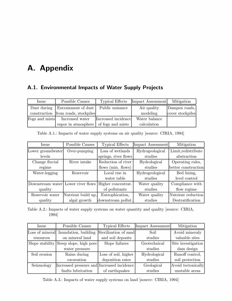
A. Appendix
A.1. Environmental Impacts of Water Supply Projects
Issue Possible Causes Typical Effects Impact Assessment Mitigation
Dust during Entrainment of dust Public nuisance Air quality Dampen roads,
construction from roads, stockpiles modeling cover stockpiles
Fogs and mists Increased water Increased incidence Water balance
vapor in atmosphere of fogs and mists calculation
Table A.1.: Impacts of water supply systems on air quality [source: CIRIA, 1994]
Issue Possible Causes Typical Effects Impact Assessment Mitigation
Lower groundwater Over-pumping Loss of wetlands Hydrogeological Limit,redistribute
levels springs, river flows studies abstraction
Change fluvial River intake Reduction of river Hydrological Operating rules,
regime flows (min. flows) studies better construction
Water-logging Reservoir Local rise in Hydrogeological Bed lining,
water table studies level control
Downstream water Lower river flows Higher concentrat. Water quality Compliance with
quality of pollutants studies flow regime
Reservoir water Nutrient build up, Eutrophication, Water quality Nutrient reduction
quality algal growth downstream pollut. studies Destratification
Table A.2.: Impacts of water supply systems on water quantity and quality [source: CIRIA,
1994]
Issue Possible Causes Typical Effects Impact Assessment Mitigation
Loss of mineral Inundation, building Sterilization of sand Soil Avoid mineraly
resources on mineral land and soil deposits studies valuable sites
Slope stability Steep slope, high pore Slope failures Geotechnical Site investigation
water pressure studies dam design
Soil erosion Rains during Loss of soil, higher Hydrological Runoff control,
excavation deposition rates studies soil protection
Seizmology Increased pressure and Increased incidence Geological Avoid tectonically
faults lubrication of earthquakes studies unstable areas
Table A.3.: Impacts of water supply systems on land [source: CIRIA, 1994]
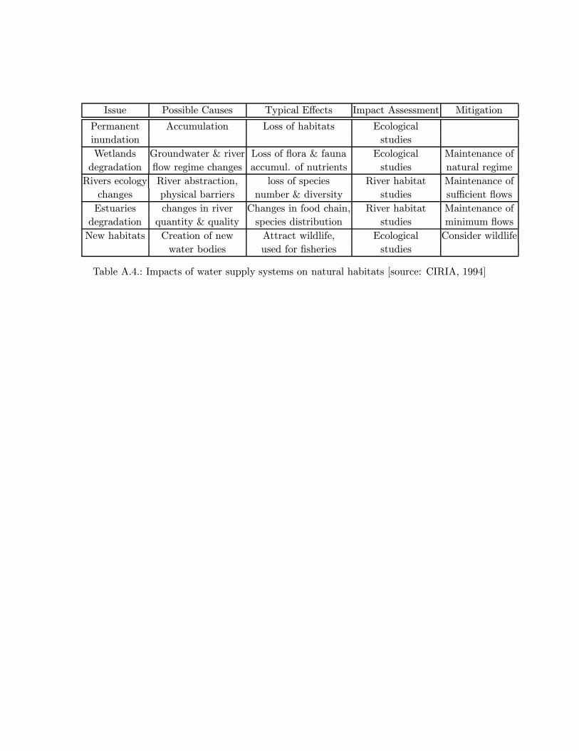
Issue Possible Causes Typical Effects Impact Assessment Mitigation
Permanent Accumulation Loss of habitats Ecological
inundation studies
Wetlands Groundwater & river Loss of flora & fauna Ecological Maintenance of
degradation flow regime changes accumul. of nutrients studies natural regime
Rivers ecology River abstraction, loss of species River habitat Maintenance of
changes physical barriers number & diversity studies sufficient flows
Estuaries changes in river Changes in food chain, River habitat Maintenance of
degradation quantity & quality species distribution studies minimum flows
New habitats Creation of new Attract wildlife, Ecological Consider wildlife
water bodies used for fisheries studies
Table A.4.: Impacts of water supply systems on natural habitats [source: CIRIA, 1994]

Institut für Wasserbau Universität Stuttgart
Pfaffenwaldring 61 70569 Stuttgart (Vaihingen) Telefon (0711) 685 - 64717/64741/64752/64679 Telefax (0711) 685 - 67020 o. 64746 o. 64681 E-Mail: [email protected] http://www.iws.uni-stuttgart.de
Direktoren Prof. Dr. rer. nat. Dr.-Ing. András Bárdossy Prof. Dr.-Ing. Rainer Helmig Prof. Dr.-Ing. Silke Wieprecht Vorstand (Stand 01.12.2006) Prof. Dr. rer. nat. Dr.-Ing. A. Bárdossy Prof. Dr.-Ing. R. Helmig Prof. Dr.-Ing. S. Wieprecht Prof. Dr.-Ing. habil. B. Westrich Jürgen Braun, PhD Dr.-Ing. H. Class Dr.-Ing. A. Färber Dr.-Ing. H.-P. Koschitzky PD Dr.-Ing. W. Marx Emeriti Prof. Dr.-Ing. Dr.-Ing. E.h. Jürgen Giesecke Prof. Dr.h.c. Dr.-Ing. E.h. Helmut Kobus, Ph.D. Lehrstuhl für Wasserbau und
Wassermengenwirtschaft Leiter: Prof. Dr.-Ing. Silke Wieprecht Stellv.: PD Dr.-Ing. Walter Marx, AOR Lehrstuhl für Hydrologie und Geohydrologie Leiter: Prof. Dr. rer. nat. Dr.-Ing. András
Bárdossy Stellv.: Dr.-Ing. Arne Färber Lehrstuhl für Hydromechanik und Hydrosystemmodellierung Leiter: Prof. Dr.-Ing. Rainer Helmig Stellv.: Dr.-Ing. Holger Class, AOR VEGAS, Versuchseinrichtung zur Grundwasser- und Altlastensanierung Leitung: Jürgen Braun, PhD
Dr.-Ing. Hans-Peter Koschitzky, AD Versuchsanstalt für Wasserbau Leiter: apl. Prof. Dr.-Ing. Bernhard Westrich
Verzeichnis der Mitteilungshefte 1 Röhnisch, Arthur: Die Bemühungen um eine Wasserbauliche Versuchsanstalt an
der Technischen Hochschule Stuttgart, und Fattah Abouleid, Abdel: Beitrag zur Berechnung einer in lockeren Sand geramm-ten, zweifach verankerten Spundwand, 1963
2 Marotz, Günter: Beitrag zur Frage der Standfestigkeit von dichten Asphaltbelägen
im Großwasserbau, 1964 3 Gurr, Siegfried: Beitrag zur Berechnung zusammengesetzter ebener Flächen-
tragwerke unter besonderer Berücksichtigung ebener Stauwände, mit Hilfe von Randwert- und Lastwertmatrizen, 1965
4 Plica, Peter: Ein Beitrag zur Anwendung von Schalenkonstruktionen im Stahlwas-
serbau, und Petrikat, Kurt: Möglichkeiten und Grenzen des wasserbaulichen Ver-suchswesens, 1966

2 Institut für Wasserbau * Universität Stuttgart * IWS 5 Plate, Erich: Beitrag zur Bestimmung der Windgeschwindigkeitsverteilung in der
durch eine Wand gestörten bodennahen Luftschicht, und Röhnisch, Arthur; Marotz, Günter: Neue Baustoffe und Bauausführungen für den Schutz der Böschungen und der Sohle von Kanälen, Flüssen und Häfen; Geste-hungskosten und jeweilige Vorteile, sowie Unny, T.E.: Schwingungs-untersuchungen am Kegelstrahlschieber, 1967
6 Seiler, Erich: Die Ermittlung des Anlagenwertes der bundeseigenen Bin-
nenschiffahrtsstraßen und Talsperren und des Anteils der Binnenschiffahrt an die-sem Wert, 1967
7 Sonderheft anläßlich des 65. Geburtstages von Prof. Arthur Röhnisch mit Beiträ-
gen von Benk, Dieter; Breitling, J.; Gurr, Siegfried; Haberhauer, Robert; Hone-kamp, Hermann; Kuz, Klaus Dieter; Marotz, Günter; Mayer-Vorfelder, Hans-Jörg; Miller, Rudolf; Plate, Erich J.; Radomski, Helge; Schwarz, Helmut; Vollmer, Ernst; Wildenhahn, Eberhard; 1967
8 Jumikis, Alfred: Beitrag zur experimentellen Untersuchung des Wassernachschubs
in einem gefrierenden Boden und die Beurteilung der Ergebnisse, 1968 9 Marotz, Günter: Technische Grundlagen einer Wasserspeicherung im natürlichen
Untergrund, 1968 10 Radomski, Helge: Untersuchungen über den Einfluß der Querschnittsform wellen-
förmiger Spundwände auf die statischen und rammtechnischen Eigenschaften, 1968
11 Schwarz, Helmut: Die Grenztragfähigkeit des Baugrundes bei Einwirkung vertikal
gezogener Ankerplatten als zweidimensionales Bruchproblem, 1969 12 Erbel, Klaus: Ein Beitrag zur Untersuchung der Metamorphose von Mittelgebirgs-
schneedecken unter besonderer Berücksichtigung eines Verfahrens zur Bestim-mung der thermischen Schneequalität, 1969
13 Westhaus, Karl-Heinz: Der Strukturwandel in der Binnenschiffahrt und sein Einfluß
auf den Ausbau der Binnenschiffskanäle, 1969 14 Mayer-Vorfelder, Hans-Jörg: Ein Beitrag zur Berechnung des Erdwiderstandes un-
ter Ansatz der logarithmischen Spirale als Gleitflächenfunktion, 1970 15 Schulz, Manfred: Berechnung des räumlichen Erddruckes auf die Wandung kreis-
zylindrischer Körper, 1970 16 Mobasseri, Manoutschehr: Die Rippenstützmauer. Konstruktion und Grenzen ihrer
Standsicherheit, 1970 17 Benk, Dieter: Ein Beitrag zum Betrieb und zur Bemessung von Hochwasser-
rückhaltebecken, 1970 18 Gàl, Attila: Bestimmung der mitschwingenden Wassermasse bei überströmten
Fischbauchklappen mit kreiszylindrischem Staublech, 1971,

Verzeichnis der Mitteilungshefte 3 19 Kuz, Klaus Dieter: Ein Beitrag zur Frage des Einsetzens von Kavitationserschei-
nungen in einer Düsenströmung bei Berücksichtigung der im Wasser gelösten Ga-se, 1971,
20 Schaak, Hartmut: Verteilleitungen von Wasserkraftanlagen, 1971 21 Sonderheft zur Eröffnung der neuen Versuchsanstalt des Instituts für Wasserbau
der Universität Stuttgart mit Beiträgen von Brombach, Hansjörg; Dirksen, Wolfram; Gàl, Attila; Gerlach, Reinhard; Giesecke, Jürgen; Holthoff, Franz-Josef; Kuz, Klaus Dieter; Marotz, Günter; Minor, Hans-Erwin; Petrikat, Kurt; Röhnisch, Arthur; Rueff, Helge; Schwarz, Helmut; Vollmer, Ernst; Wildenhahn, Eberhard; 1972
22 Wang, Chung-su: Ein Beitrag zur Berechnung der Schwingungen an Kegelstrahl-
schiebern, 1972 23 Mayer-Vorfelder, Hans-Jörg: Erdwiderstandsbeiwerte nach dem Ohde-
Variationsverfahren, 1972 24 Minor, Hans-Erwin: Beitrag zur Bestimmung der Schwingungsanfachungs-
funktionen überströmter Stauklappen, 1972, 25 Brombach, Hansjörg: Untersuchung strömungsmechanischer Elemente (Fluidik)
und die Möglichkeit der Anwendung von Wirbelkammerelementen im Wasserbau, 1972,
26 Wildenhahn, Eberhard: Beitrag zur Berechnung von Horizontalfilterbrunnen, 1972 27 Steinlein, Helmut: Die Eliminierung der Schwebstoffe aus Flußwasser zum Zweck
der unterirdischen Wasserspeicherung, gezeigt am Beispiel der Iller, 1972 28 Holthoff, Franz Josef: Die Überwindung großer Hubhöhen in der Binnenschiffahrt
durch Schwimmerhebewerke, 1973 29 Röder, Karl: Einwirkungen aus Baugrundbewegungen auf trog- und kastenförmige
Konstruktionen des Wasser- und Tunnelbaues, 1973 30 Kretschmer, Heinz: Die Bemessung von Bogenstaumauern in Abhängigkeit von
der Talform, 1973 31 Honekamp, Hermann: Beitrag zur Berechnung der Montage von Unterwasserpipe-
lines, 1973 32 Giesecke, Jürgen: Die Wirbelkammertriode als neuartiges Steuerorgan im Was-
serbau, und Brombach, Hansjörg: Entwicklung, Bauformen, Wirkungsweise und Steuereigenschaften von Wirbelkammerverstärkern, 1974
33 Rueff, Helge: Untersuchung der schwingungserregenden Kräfte an zwei hinterein-
ander angeordneten Tiefschützen unter besonderer Berücksichtigung von Kavita-tion, 1974
34 Röhnisch, Arthur: Einpreßversuche mit Zementmörtel für Spannbeton - Vergleich der Ergebnisse von Modellversuchen mit Ausführungen in Hüllwellrohren, 1975

4 Institut für Wasserbau * Universität Stuttgart * IWS 35 Sonderheft anläßlich des 65. Geburtstages von Prof. Dr.-Ing. Kurt Petrikat mit Bei-
trägen von: Brombach, Hansjörg; Erbel, Klaus; Flinspach, Dieter; Fischer jr., Ri-chard; Gàl, Attila; Gerlach, Reinhard; Giesecke, Jürgen; Haberhauer, Robert; Haf-ner Edzard; Hausenblas, Bernhard; Horlacher, Hans-Burkhard; Hutarew, Andreas; Knoll, Manfred; Krummet, Ralph; Marotz, Günter; Merkle, Theodor; Miller, Chris-toph; Minor, Hans-Erwin; Neumayer, Hans; Rao, Syamala; Rath, Paul; Rueff, Hel-ge; Ruppert, Jürgen; Schwarz, Wolfgang; Topal-Gökceli, Mehmet; Vollmer, Ernst; Wang, Chung-su; Weber, Hans-Georg; 1975
36 Berger, Jochum: Beitrag zur Berechnung des Spannungszustandes in rotations-
symmetrisch belasteten Kugelschalen veränderlicher Wandstärke unter Gas- und Flüssigkeitsdruck durch Integration schwach singulärer Differentialgleichungen, 1975
37 Dirksen, Wolfram: Berechnung instationärer Abflußvorgänge in gestauten Gerin-
nen mittels Differenzenverfahren und die Anwendung auf Hochwasserrückhalte-becken, 1976
38 Horlacher, Hans-Burkhard: Berechnung instationärer Temperatur- und Wärme-
spannungsfelder in langen mehrschichtigen Hohlzylindern, 1976 39 Hafner, Edzard: Untersuchung der hydrodynamischen Kräfte auf Baukörper im
Tiefwasserbereich des Meeres, 1977, ISBN 3-921694-39-6 40 Ruppert, Jürgen: Über den Axialwirbelkammerverstärker für den Einsatz im Was-
serbau, 1977, ISBN 3-921694-40-X 41 Hutarew, Andreas: Beitrag zur Beeinflußbarkeit des Sauerstoffgehalts in Fließge-
wässern an Abstürzen und Wehren, 1977, ISBN 3-921694-41-8, 42 Miller, Christoph: Ein Beitrag zur Bestimmung der schwingungserregenden Kräfte
an unterströmten Wehren, 1977, ISBN 3-921694-42-6 43 Schwarz, Wolfgang: Druckstoßberechnung unter Berücksichtigung der Radial- und
Längsverschiebungen der Rohrwandung, 1978, ISBN 3-921694-43-4 44 Kinzelbach, Wolfgang: Numerische Untersuchungen über den optimalen Einsatz
variabler Kühlsysteme einer Kraftwerkskette am Beispiel Oberrhein, 1978, ISBN 3-921694-44-2
45 Barczewski, Baldur: Neue Meßmethoden für Wasser-Luftgemische und deren An-
wendung auf zweiphasige Auftriebsstrahlen, 1979, ISBN 3-921694-45-0 46 Neumayer, Hans: Untersuchung der Strömungsvorgänge in radialen Wirbelkam-
merverstärkern, 1979, ISBN 3-921694-46-9 47 Elalfy, Youssef-Elhassan: Untersuchung der Strömungsvorgänge in Wirbelkam-
merdioden und -drosseln, 1979, ISBN 3-921694-47-7 48 Brombach, Hansjörg: Automatisierung der Bewirtschaftung von Wasserspeichern,
1981, ISBN 3-921694-48-5

Verzeichnis der Mitteilungshefte 5 49 Geldner, Peter: Deterministische und stochastische Methoden zur Bestimmung der
Selbstdichtung von Gewässern, 1981, ISBN 3-921694-49-3, 50 Mehlhorn, Hans: Temperaturveränderungen im Grundwasser durch Brauchwas-
sereinleitungen, 1982, ISBN 3-921694-50-7, 51 Hafner, Edzard: Rohrleitungen und Behälter im Meer, 1983, ISBN 3-921694-51-5 52 Rinnert, Bernd: Hydrodynamische Dispersion in porösen Medien: Einfluß von Dich-
teunterschieden auf die Vertikalvermischung in horizontaler Strömung, 1983, ISBN 3-921694-52-3,
53 Lindner, Wulf: Steuerung von Grundwasserentnahmen unter Einhaltung ökologi-
scher Kriterien, 1983, ISBN 3-921694-53-1, 54 Herr, Michael; Herzer, Jörg; Kinzelbach, Wolfgang; Kobus, Helmut; Rinnert, Bernd:
Methoden zur rechnerischen Erfassung und hydraulischen Sanierung von Grund-wasserkontaminationen, 1983, ISBN 3-921694-54-X
55 Schmitt, Paul: Wege zur Automatisierung der Niederschlagsermittlung, 1984, ISBN
3-921694-55-8, 56 Müller, Peter: Transport und selektive Sedimentation von Schwebstoffen bei ge-
stautem Abfluß, 1985, ISBN 3-921694-56-6 57 El-Qawasmeh, Fuad: Möglichkeiten und Grenzen der Tropfbewässerung unter be-
sonderer Berücksichtigung der Verstopfungsanfälligkeit der Tropfelemente, 1985, ISBN 3-921694-57-4,
58 Kirchenbaur, Klaus: Mikroprozessorgesteuerte Erfassung instationärer Druckfelder
am Beispiel seegangsbelasteter Baukörper, 1985, ISBN 3-921694-58-2 59 Kobus, Helmut (Hrsg.): Modellierung des großräumigen Wärme- und Schadstoff-
transports im Grundwasser, Tätigkeitsbericht 1984/85 (DFG-Forschergruppe an den Universitäten Hohenheim, Karlsruhe und Stuttgart), 1985, ISBN 3-921694-59-0,
60 Spitz, Karlheinz: Dispersion in porösen Medien: Einfluß von Inhomogenitäten und
Dichteunterschieden, 1985, ISBN 3-921694-60-4, 61 Kobus, Helmut: An Introduction to Air-Water Flows in Hydraulics, 1985,
ISBN 3-921694-61-2 62 Kaleris, Vassilios: Erfassung des Austausches von Oberflächen- und Grundwasser
in horizontalebenen Grundwassermodellen, 1986, ISBN 3-921694-62-0 63 Herr, Michael: Grundlagen der hydraulischen Sanierung verunreinigter Poren-
grundwasserleiter, 1987, ISBN 3-921694-63-9 64 Marx, Walter: Berechnung von Temperatur und Spannung in Massenbeton infolge
Hydratation, 1987, ISBN 3-921694-64-7

6 Institut für Wasserbau * Universität Stuttgart * IWS 65 Koschitzky, Hans-Peter: Dimensionierungskonzept für Sohlbelüfter in Schußrinnen
zur Vermeidung von Kavitationsschäden, 1987, ISBN 3-921694-65-5 66 Kobus, Helmut (Hrsg.): Modellierung des großräumigen Wärme- und Schadstoff-
transports im Grundwasser, Tätigkeitsbericht 1986/87 (DFG-Forschergruppe an den Universitäten Hohenheim, Karlsruhe und Stuttgart) 1987, ISBN 3-921694-66-3
67 Söll, Thomas: Berechnungsverfahren zur Abschätzung anthropogener Tempera-
turanomalien im Grundwasser, 1988, ISBN 3-921694-67-1 68 Dittrich, Andreas; Westrich, Bernd: Bodenseeufererosion, Bestandsaufnahme und
Bewertung, 1988, ISBN 3-921694-68-X, 69 Huwe, Bernd; van der Ploeg, Rienk R.: Modelle zur Simulation des Stickstoffhaus-
haltes von Standorten mit unterschiedlicher landwirtschaftlicher Nutzung, 1988, ISBN 3-921694-69-8,
70 Stephan, Karl: Integration elliptischer Funktionen, 1988, ISBN 3-921694-70-1 71 Kobus, Helmut; Zilliox, Lothaire (Hrsg.): Nitratbelastung des Grundwassers, Aus-
wirkungen der Landwirtschaft auf die Grundwasser- und Rohwasserbeschaffenheit und Maßnahmen zum Schutz des Grundwassers. Vorträge des deutsch-franzö-sischen Kolloquiums am 6. Oktober 1988, Universitäten Stuttgart und Louis Pas-teur Strasbourg (Vorträge in deutsch oder französisch, Kurzfassungen zwei-sprachig), 1988, ISBN 3-921694-71-X
72 Soyeaux, Renald: Unterströmung von Stauanlagen auf klüftigem Untergrund unter
Berücksichtigung laminarer und turbulenter Fließzustände,1991, ISBN 3-921694-72-8
73 Kohane, Roberto: Berechnungsmethoden für Hochwasserabfluß in Fließgewäs-
sern mit überströmten Vorländern, 1991, ISBN 3-921694-73-6 74 Hassinger, Reinhard: Beitrag zur Hydraulik und Bemessung von Blocksteinrampen
in flexibler Bauweise, 1991, ISBN 3-921694-74-4, 75 Schäfer, Gerhard: Einfluß von Schichtenstrukturen und lokalen Einlagerungen auf
die Längsdispersion in Porengrundwasserleitern, 1991, ISBN 3-921694-75-2 76 Giesecke, Jürgen: Vorträge, Wasserwirtschaft in stark besiedelten Regionen; Um-
weltforschung mit Schwerpunkt Wasserwirtschaft, 1991, ISBN 3-921694-76-0 77 Huwe, Bernd: Deterministische und stochastische Ansätze zur Modellierung des
Stickstoffhaushalts landwirtschaftlich genutzter Flächen auf unterschiedlichem Skalenniveau, 1992, ISBN 3-921694-77-9,
78 Rommel, Michael: Verwendung von Kluftdaten zur realitätsnahen Generierung von
Kluftnetzen mit anschließender laminar-turbulenter Strömungsberechnung, 1993, ISBN 3-92 1694-78-7
79 Marschall, Paul: Die Ermittlung lokaler Stofffrachten im Grundwasser mit Hilfe von
Einbohrloch-Meßverfahren, 1993, ISBN 3-921694-79-5,

Verzeichnis der Mitteilungshefte 7 80 Ptak, Thomas: Stofftransport in heterogenen Porenaquiferen: Felduntersuchungen
und stochastische Modellierung, 1993, ISBN 3-921694-80-9, 81 Haakh, Frieder: Transientes Strömungsverhalten in Wirbelkammern, 1993,
ISBN 3-921694-81-7 82 Kobus, Helmut; Cirpka, Olaf; Barczewski, Baldur; Koschitzky, Hans-Peter: Ver-
sucheinrichtung zur Grundwasser und Altlastensanierung VEGAS, Konzeption und Programmrahmen, 1993, ISBN 3-921694-82-5
83 Zang, Weidong: Optimaler Echtzeit-Betrieb eines Speichers mit aktueller Abflußre-
generierung, 1994, ISBN 3-921694-83-3, 84 Franke, Hans-Jörg: Stochastische Modellierung eines flächenhaften Stoffeintrages
und Transports in Grundwasser am Beispiel der Pflanzenschutzmittelproblematik, 1995, ISBN 3-921694-84-1
85 Lang, Ulrich: Simulation regionaler Strömungs- und Transportvorgänge in Karst-
aquiferen mit Hilfe des Doppelkontinuum-Ansatzes: Methodenentwicklung und Pa-rameteridentifikation, 1995, ISBN 3-921694-85-X,
86 Helmig, Rainer: Einführung in die Numerischen Methoden der Hydromechanik,
1996, ISBN 3-921694-86-8, 87 Cirpka, Olaf: CONTRACT: A Numerical Tool for Contaminant Transport and
Chemical Transformations - Theory and Program Documentation -, 1996, ISBN 3-921694-87-6
88 Haberlandt, Uwe: Stochastische Synthese und Regionalisierung des Niederschla-
ges für Schmutzfrachtberechnungen, 1996, ISBN 3-921694-88-4 89 Croisé, Jean: Extraktion von flüchtigen Chemikalien aus natürlichen Lockergestei-
nen mittels erzwungener Luftströmung, 1996, ISBN 3-921694-89-2, 90 Jorde, Klaus: Ökologisch begründete, dynamische Mindestwasserregelungen bei
Ausleitungskraftwerken, 1997, ISBN 3-921694-90-6, 91 Helmig, Rainer: Gekoppelte Strömungs- und Transportprozesse im Untergrund -
Ein Beitrag zur Hydrosystemmodellierung-, 1998, ISBN 3-921694-91-4 92 Emmert, Martin: Numerische Modellierung nichtisothermer Gas-Wasser Systeme
in porösen Medien, 1997, ISBN 3-921694-92-2 93 Kern, Ulrich: Transport von Schweb- und Schadstoffen in staugeregelten Fließge-
wässern am Beispiel des Neckars, 1997, ISBN 3-921694-93-0, 94 Förster, Georg: Druckstoßdämpfung durch große Luftblasen in Hochpunkten von
Rohrleitungen 1997, ISBN 3-921694-94-9 95 Cirpka, Olaf: Numerische Methoden zur Simulation des reaktiven Mehrkomponen-
tentransports im Grundwasser, 1997, ISBN 3-921694-95-7,

8 Institut für Wasserbau * Universität Stuttgart * IWS 96 Färber, Arne: Wärmetransport in der ungesättigten Bodenzone: Entwicklung einer
thermischen In-situ-Sanierungstechnologie, 1997, ISBN 3-921694-96-5 97 Betz, Christoph: Wasserdampfdestillation von Schadstoffen im porösen Medium:
Entwicklung einer thermischen In-situ-Sanierungstechnologie, 1998, ISBN 3-921694-97-3
98 Xu, Yichun: Numerical Modeling of Suspended Sediment Transport in Rivers,
1998, ISBN 3-921694-98-1, 99 Wüst, Wolfgang: Geochemische Untersuchungen zur Sanierung CKW-
kontaminierter Aquifere mit Fe(0)-Reaktionswänden, 2000, ISBN 3-933761-02-2 100 Sheta, Hussam: Simulation von Mehrphasenvorgängen in porösen Medien unter
Einbeziehung von Hysterese-Effekten, 2000, ISBN 3-933761-03-4 101 Ayros, Edwin: Regionalisierung extremer Abflüsse auf der Grundlage statistischer
Verfahren, 2000, ISBN 3-933761-04-2, 102 Huber, Ralf: Compositional Multiphase Flow and Transport in Heterogeneous Po-
rous Media, 2000, ISBN 3-933761-05-0 103 Braun, Christopherus: Ein Upscaling-Verfahren für Mehrphasenströmungen in po-
rösen Medien, 2000, ISBN 3-933761-06-9 104 Hofmann, Bernd: Entwicklung eines rechnergestützten Managementsystems zur
Beurteilung von Grundwasserschadensfällen, 2000, ISBN 3-933761-07-7 105 Class, Holger: Theorie und numerische Modellierung nichtisothermer Mehrphasen-
prozesse in NAPL-kontaminierten porösen Medien, 2001, ISBN 3-933761-08-5
106 Schmidt, Reinhard: Wasserdampf- und Heißluftinjektion zur thermischen Sanie-
rung kontaminierter Standorte, 2001, ISBN 3-933761-09-3 107 Josef, Reinhold:, Schadstoffextraktion mit hydraulischen Sanierungsverfahren un-
ter Anwendung von grenzflächenaktiven Stoffen, 2001, ISBN 3-933761-10-7 108 Schneider, Matthias: Habitat- und Abflussmodellierung für Fließgewässer mit un-
scharfen Berechnungsansätzen, 2001, ISBN 3-933761-11-5 109 Rathgeb, Andreas: Hydrodynamische Bemessungsgrundlagen für Lockerdeckwer-
ke an überströmbaren Erddämmen, 2001, ISBN 3-933761-12-3 110 Lang, Stefan: Parallele numerische Simulation instätionärer Probleme mit adapti-
ven Methoden auf unstrukturierten Gittern, 2001, ISBN 3-933761-13-1 111 Appt, Jochen; Stumpp Simone: Die Bodensee-Messkampagne 2001, IWS/CWR
Lake Constance Measurement Program 2001, 2002, ISBN 3-933761-14-X 112 Heimerl, Stephan: Systematische Beurteilung von Wasserkraftprojekten, 2002,
ISBN 3-933761-15-8
Verzeichnis der Mitteilungshefte 9 113 Iqbal, Amin: On the Management and Salinity Control of Drip Irrigation, 2002, ISBN
3-933761-16-6 114 Silberhorn-Hemminger, Annette: Modellierung von Kluftaquifersystemen: Geosta-
tistische Analyse und deterministisch-stochastische Kluftgenerierung, 2002, ISBN 3-933761-17-4
115 Winkler, Angela: Prozesse des Wärme- und Stofftransports bei der In-situ-
Sanierung mit festen Wärmequellen, 2003, ISBN 3-933761-18-2 116 Marx, Walter: Wasserkraft, Bewässerung, Umwelt - Planungs- und Bewertungs-
schwerpunkte der Wasserbewirtschaftung, 2003, ISBN 3-933761-19-0 117 Hinkelmann, Reinhard: Efficient Numerical Methods and Information-Processing
Techniques in Environment Water, 2003, ISBN 3-933761-20-4 118 Samaniego-Eguiguren, Luis Eduardo: Hydrological Consequences of Land Use /
Land Cover and Climatic Changes in Mesoscale Catchments, 2003, ISBN 3-933761-21-2
119 Neunhäuserer, Lina: Diskretisierungsansätze zur Modellierung von Strömungs-
und Transportprozessen in geklüftet-porösen Medien, 2003, ISBN 3-933761-22-0 120 Paul, Maren: Simulation of Two-Phase Flow in Heterogeneous Poros Media with
Adaptive Methods, 2003, ISBN 3-933761-23-9 121 Ehret, Uwe: Rainfall and Flood Nowcasting in Small Catchments using Weather
Radar, 2003, ISBN 3-933761-24-7 122 Haag, Ingo: Der Sauerstoffhaushalt staugeregelter Flüsse am Beispiel des Ne-
ckars - Analysen, Experimente, Simulationen -, 2003, ISBN 3-933761-25-5 123 Appt, Jochen: Analysis of Basin-Scale Internal Waves in Upper Lake Constance,
2003, ISBN 3-933761-26-3 124 Hrsg.: Schrenk, Volker; Batereau, Katrin; Barczewski, Baldur; Weber, Karolin und
Koschitzky, Hans-Peter: Symposium Ressource Fläche und VEGAS - Statuskol-loquium 2003, 30. September und 1. Oktober 2003, 2003, ISBN 3-933761-27-1
125 Omar Khalil Ouda: Optimisation of Agricultural Water Use: A Decision Support
System for the Gaza Strip, 2003, ISBN 3-933761-28-0 126 Batereau, Katrin: Sensorbasierte Bodenluftmessung zur Vor-Ort-Erkundung von
Schadensherden im Untergrund, 2004, ISBN 3-933761-29-8 127 Witt, Oliver: Erosionsstabilität von Gewässersedimenten mit Auswirkung auf den
Stofftransport bei Hochwasser am Beispiel ausgewählter Stauhaltungen des Ober-rheins, 2004, ISBN 3-933761-30-1
128 Jakobs, Hartmut: Simulation nicht-isothermer Gas-Wasser-Prozesse in komplexen
Kluft-Matrix-Systemen, 2004, ISBN 3-933761-31-X
10 Institut für Wasserbau * Universität Stuttgart * IWS 129 Li, Chen-Chien: Deterministisch-stochastisches Berechnungskonzept zur Beurtei-
lung der Auswirkungen erosiver Hochwasserereignisse in Flussstauhaltungen, 2004, ISBN 3-933761-32-8
130 Reichenberger, Volker; Helmig, Rainer; Jakobs, Hartmut; Bastian, Peter; Niessner,
Jennifer: Complex Gas-Water Processes in Discrete Fracture-Matrix Systems: Up-scaling, Mass-Conservative Discretization and Efficient Multilevel Solution, 2004, ISBN 3-933761-33-6
131 Hrsg.: Barczewski, Baldur; Koschitzky, Hans-Peter; Weber, Karolin; Wege, Ralf:
VEGAS - Statuskolloquium 2004, Tagungsband zur Veranstaltung am 05. Oktober 2004 an der Universität Stuttgart, Campus Stuttgart-Vaihingen, 2004, ISBN 3-933761-34-4
132 Asie, Kemal Jabir: Finite Volume Models for Multiphase Multicomponent Flow
through Porous Media. 2005, ISBN 3-933761-35-2 133 Jacoub, George: Development of a 2-D Numerical Module for Particulate Con-
taminant Transport in Flood Retention Reservoirs and Impounded Rivers, 2004, ISBN 3-933761-36-0
134 Nowak, Wolfgang: Geostatistical Methods for the Identification of Flow and Trans-
port Parameters in the Subsurface, 2005, ISBN 3-933761-37-9 135 Süß, Mia: Analysis of the influence of structures and boundaries on flow and
transport processes in fractured porous media, 2005, ISBN 3-933761-38-7 136 Jose, Surabhin Chackiath: Experimental Investigations on Longitudinal Dispersive
Mixing in Heterogeneous Aquifers, 2005, ISBN: 3-933761-39-5 137 Filiz, Fulya: Linking Large-Scale Meteorological Conditions to Floods in Mesoscale
Catchments, 2005, ISBN 3-933761-40-9 138 Qin, Minghao: Wirklichkeitsnahe und recheneffiziente Ermittlung von Temperatur
und Spannungen bei großen RCC-Staumauern, 2005, ISBN 3-933761-41-7 139 Kobayashi, Kenichiro: Optimization Methods for Multiphase Systems in the Sub-
surface - Application to Methane Migration in Coal Mining Areas, 2005, ISBN 3-933761-42-5
140 Rahman, Md. Arifur: Experimental Investigations on Transverse Dispersive Mixing
in Heterogeneous Porous Media, 2005, ISBN 3-933761-43-3 141 Schrenk, Volker: Ökobilanzen zur Bewertung von Altlastensanierungsmaßnahmen,
2005, ISBN 3-933761-44-1 142 Hundecha, Hirpa Yeshewatesfa: Regionalization of Parameters of a Conceptual
Rainfall-Runoff Model, 2005, ISBN: 3-933761-45-X 143 Wege, Ralf: Untersuchungs- und Überwachungsmethoden für die Beurteilung na-
türlicher Selbstreinigungsprozesse im Grundwasser, 2005, ISBN 3-933761-46-8

Verzeichnis der Mitteilungshefte 11 144 Breiting, Thomas: Techniken und Methoden der Hydroinformatik - Modellierung
von komplexen Hydrosystemen im Untergrund, 2006, 3-933761-47-6 145 Hrsg.: Braun, Jürgen; Koschitzky, Hans-Peter; Müller, Martin: Ressource Unter-
grund: 10 Jahre VEGAS: Forschung und Technologieentwicklung zum Schutz von Grundwasser und Boden, Tagungsband zur Veranstaltung am 28. und 29. Sep-tember 2005 an der Universität Stuttgart, Campus Stuttgart-Vaihingen, 2005, ISBN 3-933761-48-4
146 Rojanschi, Vlad: Abflusskonzentration in mesoskaligen Einzugsgebieten unter
Berücksichtigung des Sickerraumes, 2006, ISBN 3-933761-49-2 147 Winkler, Nina Simone: Optimierung der Steuerung von Hochwasserrückhaltebe-
cken-systemen, 2006, ISBN 3-933761-50-6 148 Wolf, Jens: Räumlich differenzierte Modellierung der Grundwasserströmung allu-
vialer Aquifere für mesoskalige Einzugsgebiete, 2006, ISBN: 3-933761-51-4 149 Kohler, Beate: Externe Effekte der Laufwasserkraftnutzung, 2006,
ISBN 3-933761-52-2 150 Hrsg.: Braun, Jürgen; Koschitzky, Hans-Peter; Stuhrmann, Matthias: VEGAS-
Statuskolloquium 2006, Tagungsband zur Veranstaltung am 28. September 2006 an der Universität Stuttgart, Campus Stuttgart-Vaihingen, 2006, ISBN 3-933761-53-0
151 Niessner, Jennifer: Multi-Scale Modeling of Multi-Phase - Multi-Component Pro-
cesses in Heterogeneous Porous Media, 2006, ISBN 3-933761-54-9 152 Fischer, Markus: Beanspruchung eingeerdeter Rohrleitungen infolge Austrocknung
bindiger Böden, 2006, ISBN 3-933761-55-7 153 Schneck, Alexander: Optimierung der Grundwasserbewirtschaftung unter Berück-
sichtigung der Belange der Wasserversorgung, der Landwirtschaft und des Natur-schutzes, 2006, ISBN 3-933761-56-5
154 Das, Tapash: The Impact of Spatial Variability of Precipitation on the Predictive
Uncertainty of Hydrological Models, 2006, ISBN 3-933761-57-3 155 Bielinski, Andreas: Numerical Simulation of CO2 sequestration in geological forma-
tions, 2007, ISBN 3-933761-58-1 156 Mödinger, Jens: Entwicklung eines Bewertungs- und Entscheidungsunterstüt-
zungssystems für eine nachhaltige regionale Grundwasserbewirtschaftung, 2006, ISBN 3-933761-60-3
157 Manthey, Sabine: Two-phase flow processes with dynamic effects in porous
media - parameter estimation and simulation, 2007, ISBN 3-933761-61-1 158 Pozos Estrada, Oscar: Investigation on the Effects of Entrained Air in Pipelines,
2007, ISBN 3-933761-62-X

12 Institut für Wasserbau * Universität Stuttgart * IWS 159 Ochs, Steffen Oliver: Steam injection into saturated porous media – process
analysis including experimental and numerical investigations, 2007, ISBN 3-933761-63-8
160 Marx, Andreas: Einsatz gekoppelter Modelle und Wetterradar zur Abschätzung
von Niederschlagsintensitäten und zur Abflussvorhersage, 2007, ISBN 3-933761-64-6
161 Hartmann, Gabriele Maria: Investigation of Evapotranspiration Concepts in Hydro-
logical Modelling for Climate Change Impact Assessment, 2007, ISBN 3-933761-65-4
162 Kebede Gurmessa, Tesfaye: Numerical Investigation on Flow and Transport Char-
acteristics to Improve Long-Term Simulation of Reservoir Sedimentation, 2007, ISBN 3-933761-66-2
163 Trifković, Aleksandar: Multi-objective and Risk-based Modelling Methodology for
Planning, Design and Operation of Water Supply Systems, 2007, 3-933761-67-0 Die Mitteilungshefte ab dem Jahr 2005 stehen als pdf-Datei über die Homepage des In-stituts: www.iws.uni-stuttgart.de zur Verfügung.