BIS Papers No 49 129
Assessing inflationary pressures in Colombia
Hernando Vargas, Andrés González, Eliana González, José Vicente Romero and Luis Eduardo Rojas
1. Introduction
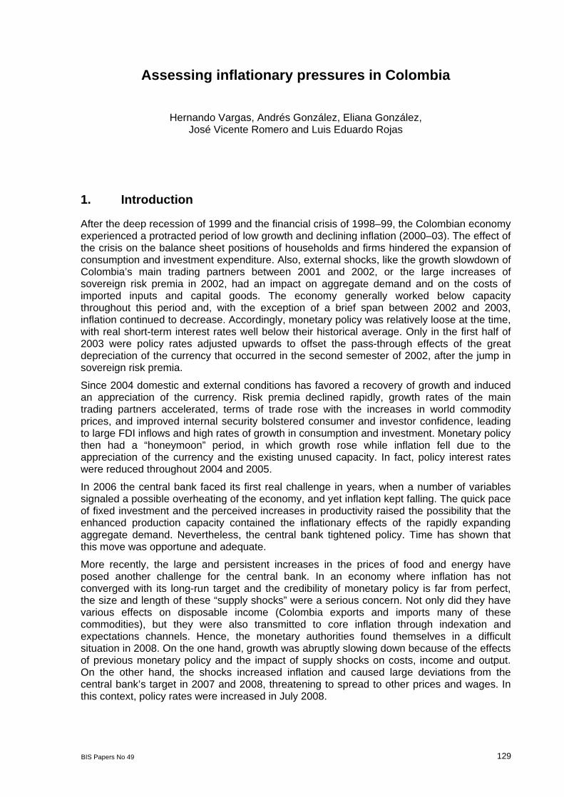
After the deep recession of 1999 and the financial crisis of 1998–99, the Colombian economy experienced a protracted period of low growth and declining inflation (2000–03). The effect of the crisis on the balance sheet positions of households and firms hindered the expansion of consumption and investment expenditure. Also, external shocks, like the growth slowdown of Colombia’s main trading partners between 2001 and 2002, or the large increases of sovereign risk premia in 2002, had an impact on aggregate demand and on the costs of imported inputs and capital goods. The economy generally worked below capacity throughout this period and, with the exception of a brief span between 2002 and 2003, inflation continued to decrease. Accordingly, monetary policy was relatively loose at the time, with real short-term interest rates well below their historical average. Only in the first half of 2003 were policy rates adjusted upwards to offset the pass-through effects of the great depreciation of the currency that occurred in the second semester of 2002, after the jump in sovereign risk premia.
Since 2004 domestic and external conditions has favored a recovery of growth and induced an appreciation of the currency. Risk premia declined rapidly, growth rates of the main trading partners accelerated, terms of trade rose with the increases in world commodity prices, and improved internal security bolstered consumer and investor confidence, leading to large FDI inflows and high rates of growth in consumption and investment. Monetary policy then had a “honeymoon” period, in which growth rose while inflation fell due to the appreciation of the currency and the existing unused capacity. In fact, policy interest rates were reduced throughout 2004 and 2005.
In 2006 the central bank faced its first real challenge in years, when a number of variables signaled a possible overheating of the economy, and yet inflation kept falling. The quick pace of fixed investment and the perceived increases in productivity raised the possibility that the enhanced production capacity contained the inflationary effects of the rapidly expanding aggregate demand. Nevertheless, the central bank tightened policy. Time has shown that this move was opportune and adequate.
More recently, the large and persistent increases in the prices of food and energy have posed another challenge for the central bank. In an economy where inflation has not converged with its long-run target and the credibility of monetary policy is far from perfect, the size and length of these “supply shocks” were a serious concern. Not only did they have various effects on disposable income (Colombia exports and imports many of these commodities), but they were also transmitted to core inflation through indexation and expectations channels. Hence, the monetary authorities found themselves in a difficult situation in 2008. On the one hand, growth was abruptly slowing down because of the effects of previous monetary policy and the impact of supply shocks on costs, income and output. On the other hand, the shocks increased inflation and caused large deviations from the central bank’s target in 2007 and 2008, threatening to spread to other prices and wages. In this context, policy rates were increased in July 2008.
130 BIS Papers No 49
This paper describes these challenges and explains the reaction of the central bank. In the case of the 2006 episode, emphasis is placed on the information provided by productivity and unit labor costs statistics in detecting inflationary pressures. It is apparent that the cyclical components embedded in these series limit their usefulness and, in the absence of models that allow us to understand their behavior, they must be examined within a wider array of macroeconomic and financial variables.
For the 2007–08 episode, the discussion focuses on the role of core inflation measures, some of which are evaluated according to the standard criteria. No particular measure seems to be clearly superior to the others, a result similar to that found by Rich and Steindel (2007), who explain this as a reflection of the varying nature of the transitory shocks hitting inflation. Consequently, we argue that the monitoring of core inflation measures must be complemented with an assessment of the nature of the inflation shocks and an analysis of the transmission of the transitory shocks to macroeconomic inflation. We explore this transmission in the final part of the paper by examining the determination of inflation expectations, the effects of transitory inflation shocks on inflation expectations and the impact of shocks to subsets of the consumer price index (CPI) basket on other subsets and the overall CPI.
2. 2006: detecting an overheating economy
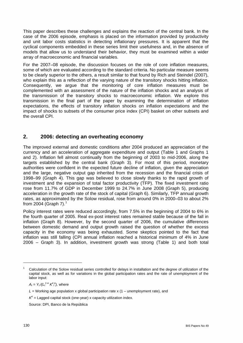
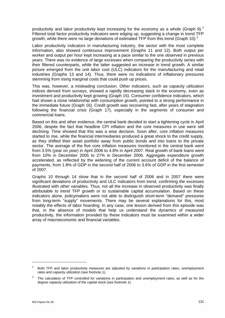
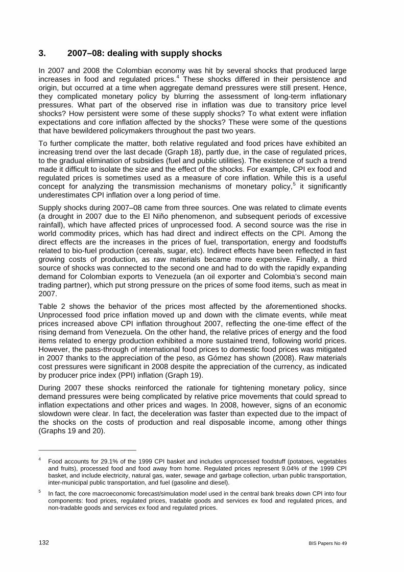
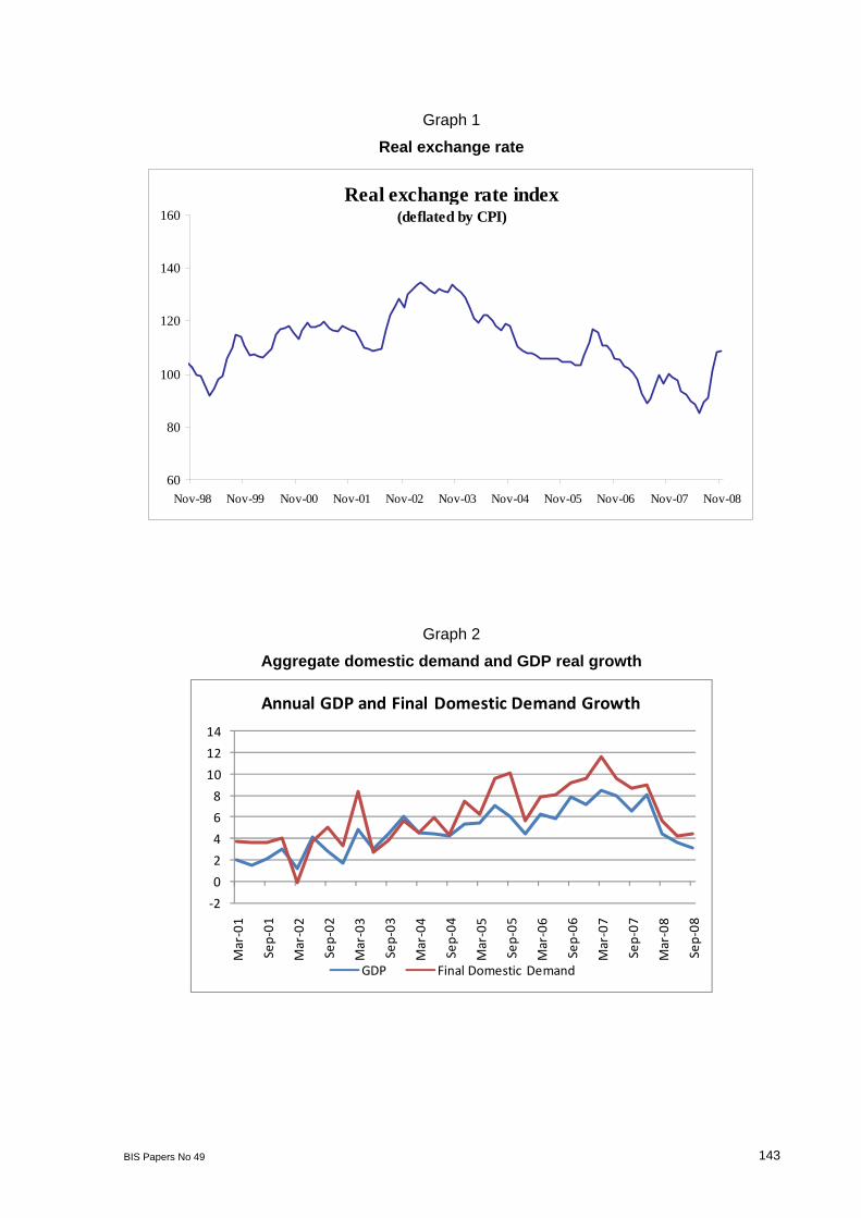
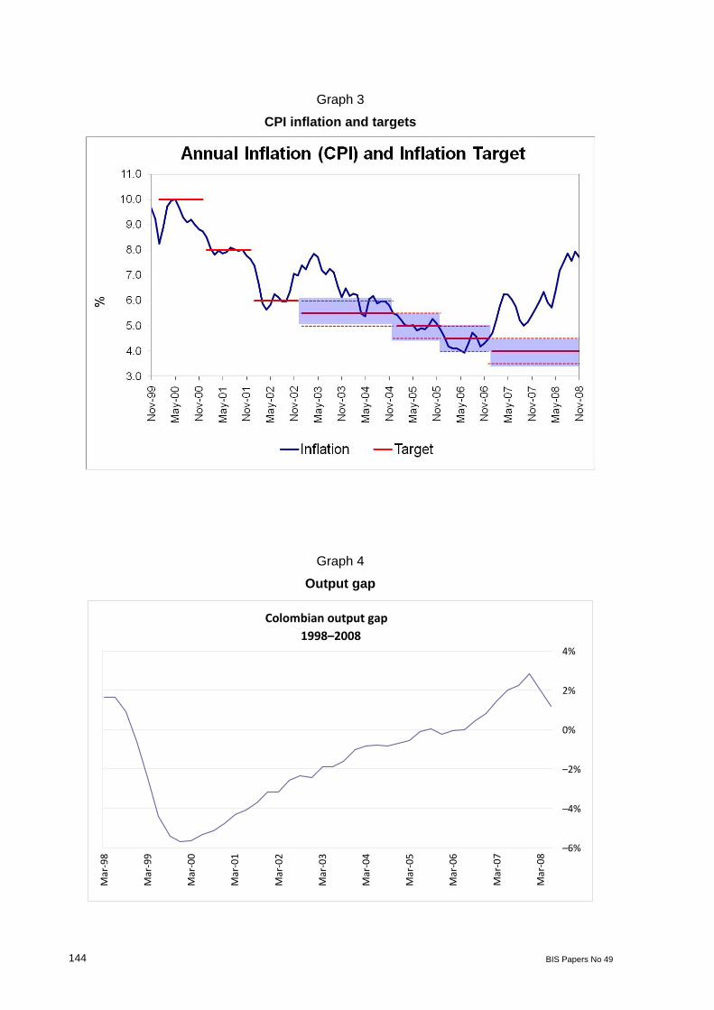
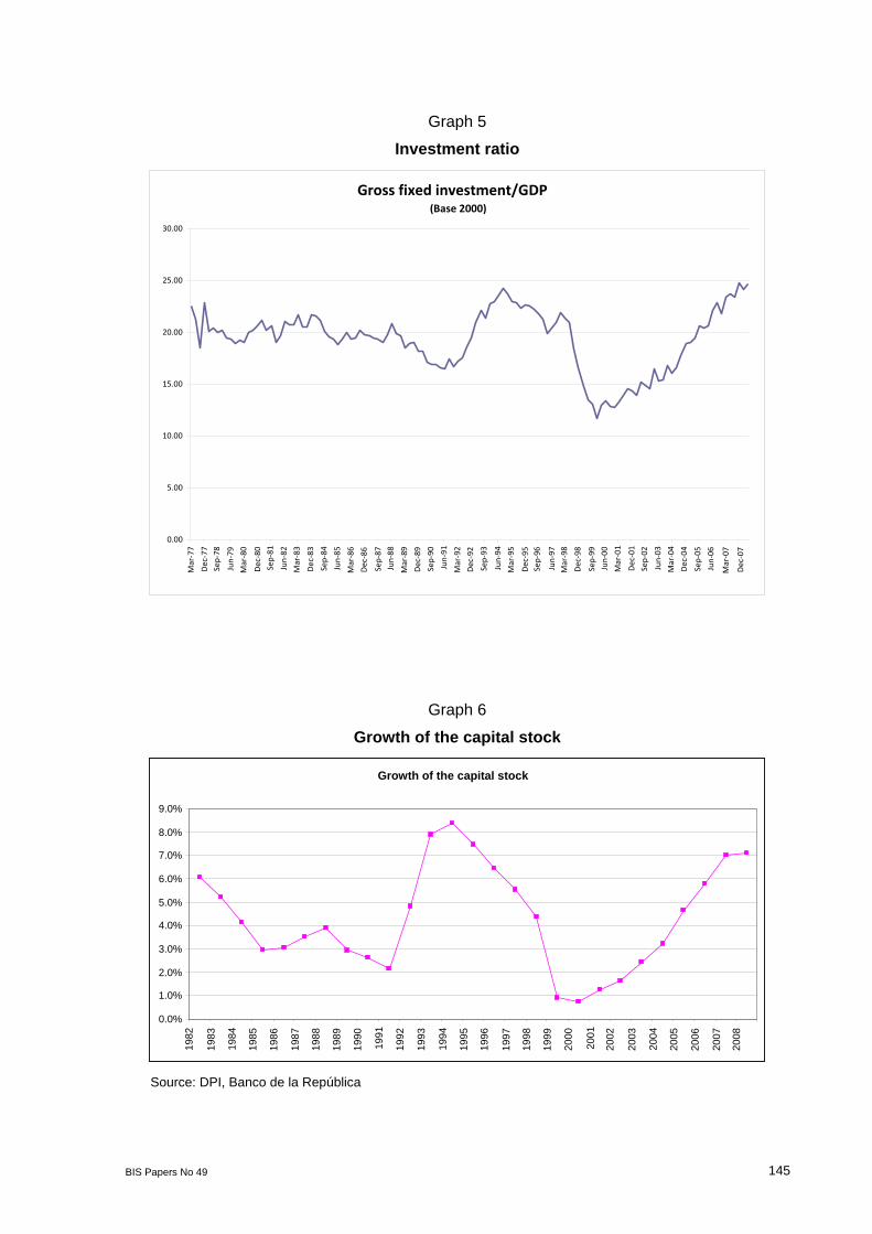
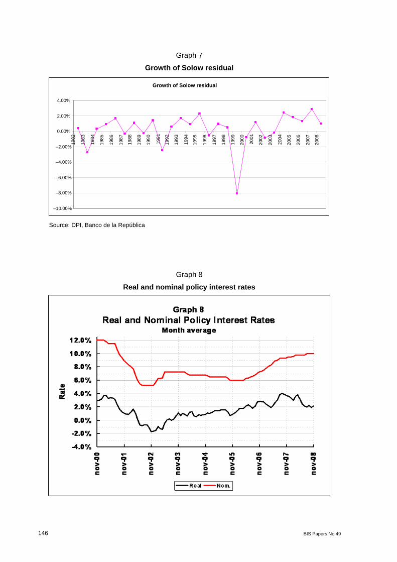
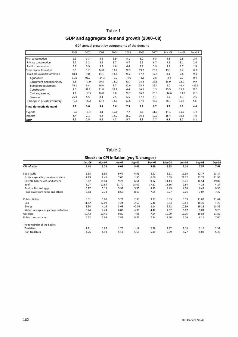
The improved external and domestic conditions after 2004 produced an appreciation of the currency and an acceleration of aggregate expenditure and output (Table 1 and Graphs 1 and 2). Inflation fell almost continually from the beginning of 2003 to mid-2006, along the targets established by the central bank (Graph 3). For most of this period, monetary authorities were confident in the expected future decline of inflation, given the appreciation and the large, negative output gap inherited from the recession and the financial crisis of 1998–99 (Graph 4). This gap was believed to close slowly thanks to the rapid growth of investment and the expansion of total factor productivity (TFP). The fixed investment ratio rose from 11.7% of GDP in December 1999 to 24.7% in June 2008 (Graph 5), producing acceleration in the growth rate of the stock of capital (Graph 6). Similarly, TFP annual growth rates, as approximated by the Solow residual, rose from around 0% in 2000–03 to about 2% from 2004 (Graph 7).1
Policy interest rates were reduced accordingly, from 7.5% in the beginning of 2004 to 6% in the fourth quarter of 2005. Real ex-post interest rates remained stable because of the fall in inflation (Graph 8). However, by the second quarter of 2006, the cumulative differences between domestic demand and output growth raised the question of whether the excess capacity in the economy was being exhausted. Some skeptics pointed to the fact that inflation was still falling (CPI annual inflation reached a historical minimum of 4% in June 2006 – Graph 3). In addition, investment growth was strong (Table 1) and both total
1 Calculation of the Solow residual series controlled for delays in installation and the degree of utilization of the
capital stock, as well as for variations in the global participation rates and the rate of unemployment of the labor input:
At = Yt /(Lt1-a Ke
ta), where
L = Working age population x global participation rate x (1 – unemployment rate), and
Ke = Lagged capital stock (one-year) x capacity utilization index.
Source: DPI, Banco de la República
BIS Papers No 49 131
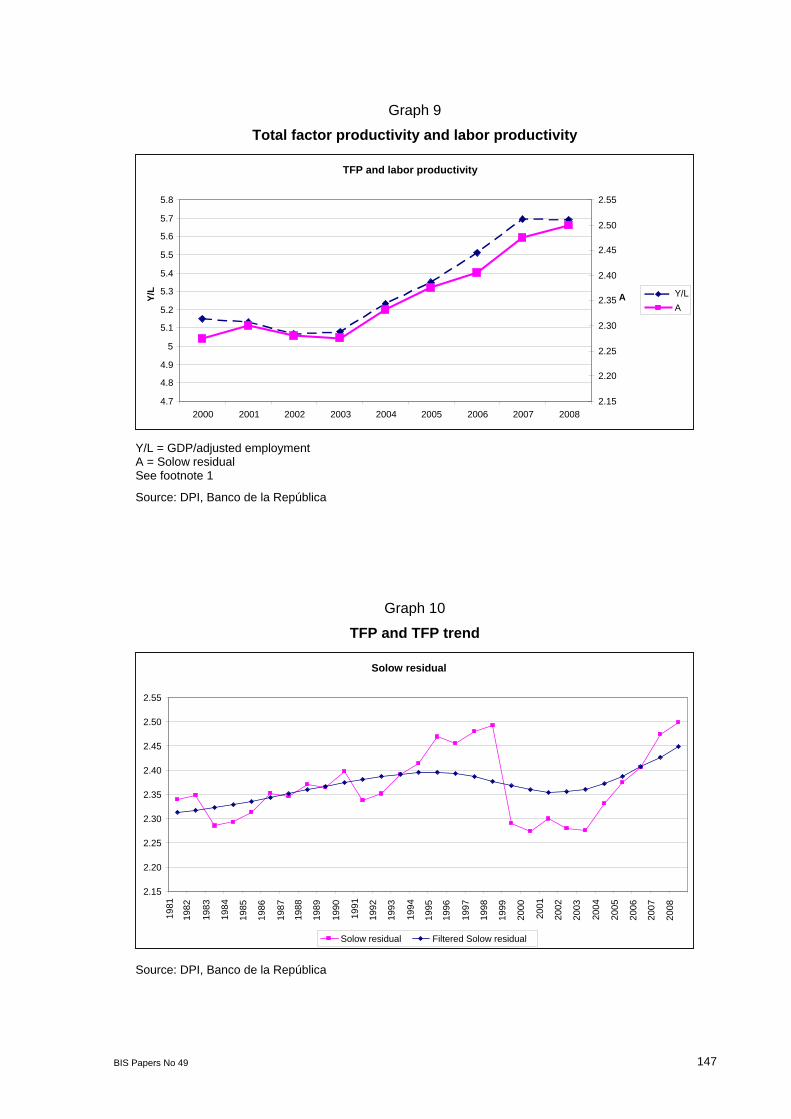
productivity and labor productivity kept increasing for the economy as a whole (Graph 9).2 Filtered total factor productivity indicators were edging up, suggesting a change in trend TFP growth, while there were no large deviations of estimated TFP from this trend (Graph 10).3
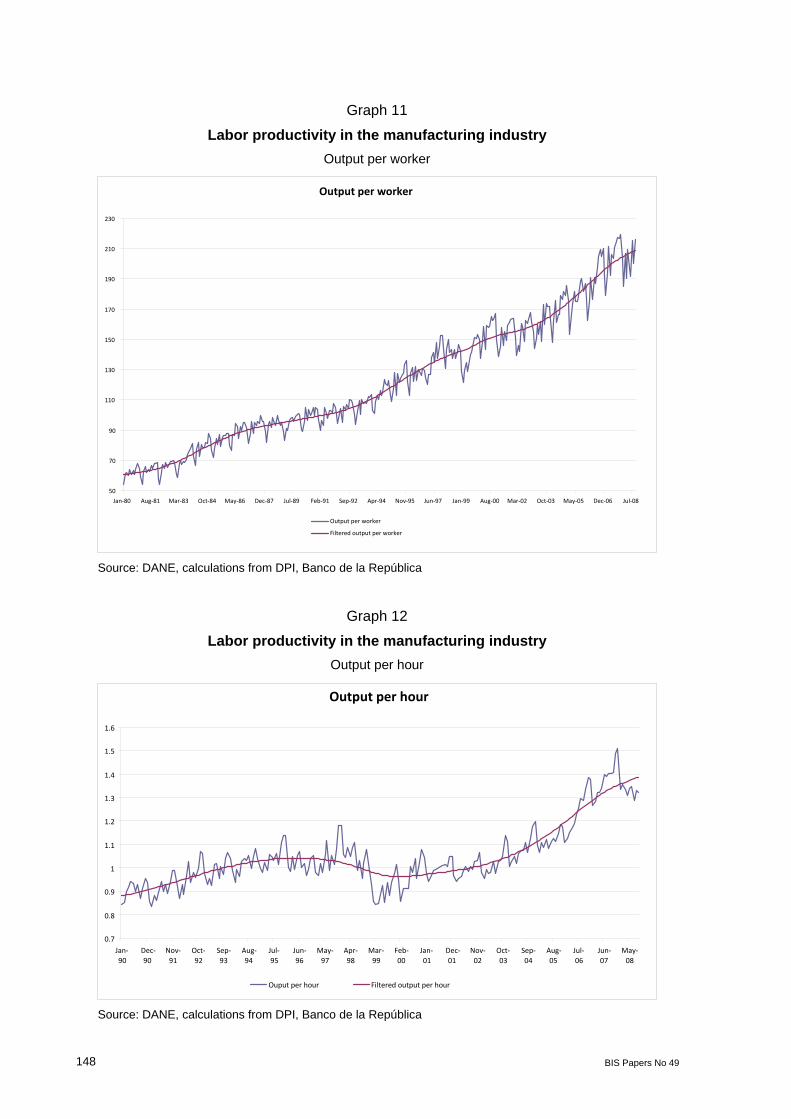
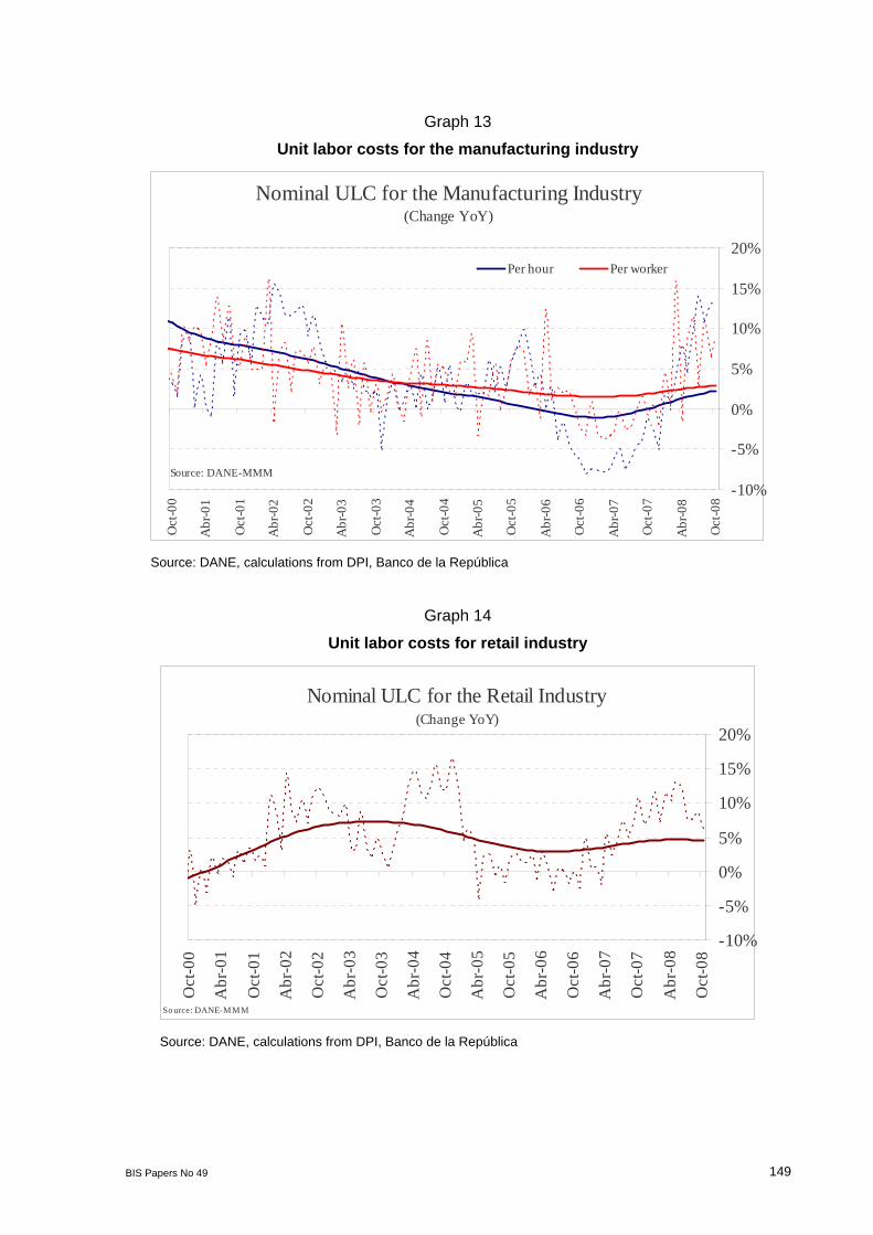
Labor productivity indicators in manufacturing industry, the sector with the most complete information, also showed continuous improvement (Graphs 11 and 12). Both output per worker and output per hour kept increasing at a pace similar to the one observed in previous years. There was no evidence of large excesses when comparing the productivity series with their filtered counterparts, while the latter suggested an increase in trend growth. A similar picture emerged from the unit labor cost (ULC) indicators for the manufacturing and retail industries (Graphs 13 and 14). Thus, there were no indications of inflationary pressures stemming from rising marginal costs that could push up prices.
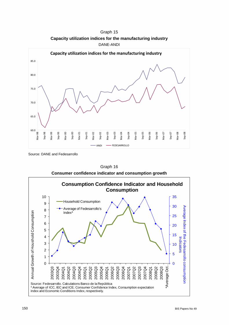
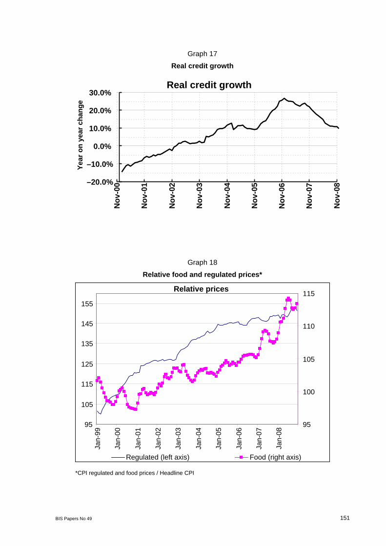
This was, however, a misleading conclusion. Other indicators, such as capacity utilization indices derived from surveys, showed a rapidly decreasing slack in the economy, even as investment and productivity kept growing (Graph 15). Consumer confidence indicators, which had shown a close relationship with consumption growth, pointed to a strong performance in the immediate future (Graph 16). Credit growth was recovering fast, after years of stagnation following the financial crisis (Graph 17), especially in the segments of consumer and commercial loans.
Based on this and other evidence, the central bank decided to start a tightening cycle in April 2006, despite the fact that headline CPI inflation and the core measures in use were still declining. Time showed that this was a wise decision. Soon after, core inflation measures started to rise, while the financial intermediaries produced a great shock to the credit supply, as they shifted their asset portfolio away from public bonds and into loans to the private sector. The average of the five core inflation measures monitored in the central bank went from 3.5% (year on year) in April 2006 to 4.8% in April 2007. Real growth of bank loans went from 10% in December 2005 to 27% in December 2006. Aggregate expenditure growth accelerated, as reflected by the widening of the current account deficit of the balance of payments, from 1.8% of GDP in the second half of 2006 to 3.6% of GDP in the first semester of 2007.
Graphs 10 through 14 show that in the second half of 2006 and in 2007 there were significant deviations of productivity and ULC indicators from trend, confirming the excesses illustrated with other variables. Thus, not all the increase in observed productivity was finally attributable to trend TFP growth or to sustainable capital accumulation. Based on these indicators alone, policymakers were not able to distinguish short-term “demand” pressures from long-term “supply” movements. There may be several explanations for this, most notably the effects of labor hoarding. In any case, one lesson derived from this episode was that, in the absence of models that help us understand the dynamics of measured productivity, the information provided by these indicators must be examined within a wider array of macroeconomic and financial variables.
2 Both TFP and labor productivity measures are adjusted by variations in participation rates, unemployment
rates and capacity utilization (see footnote 1). 3 The calculation of TFP controlled for variations in participation and unemployment rates, as well as for the
degree capacity utilization of the capital stock (see footnote 1).
132 BIS Papers No 49
3. 2007–08: dealing with supply shocks
In 2007 and 2008 the Colombian economy was hit by several shocks that produced large increases in food and regulated prices.4 These shocks differed in their persistence and origin, but occurred at a time when aggregate demand pressures were still present. Hence, they complicated monetary policy by blurring the assessment of long-term inflationary pressures. What part of the observed rise in inflation was due to transitory price level shocks? How persistent were some of these supply shocks? To what extent were inflation expectations and core inflation affected by the shocks? These were some of the questions that have bewildered policymakers throughout the past two years.
To further complicate the matter, both relative regulated and food prices have exhibited an increasing trend over the last decade (Graph 18), partly due, in the case of regulated prices, to the gradual elimination of subsidies (fuel and public utilities). The existence of such a trend made it difficult to isolate the size and the effect of the shocks. For example, CPI ex food and regulated prices is sometimes used as a measure of core inflation. While this is a useful concept for analyzing the transmission mechanisms of monetary policy,5 it significantly underestimates CPI inflation over a long period of time.
Supply shocks during 2007–08 came from three sources. One was related to climate events (a drought in 2007 due to the El Niño phenomenon, and subsequent periods of excessive rainfall), which have affected prices of unprocessed food. A second source was the rise in world commodity prices, which has had direct and indirect effects on the CPI. Among the direct effects are the increases in the prices of fuel, transportation, energy and foodstuffs related to bio-fuel production (cereals, sugar, etc). Indirect effects have been reflected in fast growing costs of production, as raw materials became more expensive. Finally, a third source of shocks was connected to the second one and had to do with the rapidly expanding demand for Colombian exports to Venezuela (an oil exporter and Colombia’s second main trading partner), which put strong pressure on the prices of some food items, such as meat in 2007.
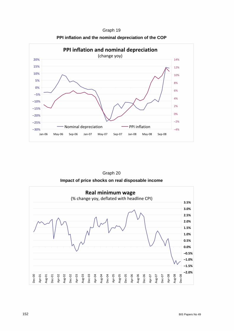
Table 2 shows the behavior of the prices most affected by the aforementioned shocks. Unprocessed food price inflation moved up and down with the climate events, while meat prices increased above CPI inflation throughout 2007, reflecting the one-time effect of the rising demand from Venezuela. On the other hand, the relative prices of energy and the food items related to energy production exhibited a more sustained trend, following world prices. However, the pass-through of international food prices to domestic food prices was mitigated in 2007 thanks to the appreciation of the peso, as Gómez has shown (2008). Raw materials cost pressures were significant in 2008 despite the appreciation of the currency, as indicated by producer price index (PPI) inflation (Graph 19).
During 2007 these shocks reinforced the rationale for tightening monetary policy, since demand pressures were being complicated by relative price movements that could spread to inflation expectations and other prices and wages. In 2008, however, signs of an economic slowdown were clear. In fact, the deceleration was faster than expected due to the impact of the shocks on the costs of production and real disposable income, among other things (Graphs 19 and 20).
4 Food accounts for 29.1% of the 1999 CPI basket and includes unprocessed foodstuff (potatoes, vegetables
and fruits), processed food and food away from home. Regulated prices represent 9.04% of the 1999 CPI basket, and include electricity, natural gas, water, sewage and garbage collection, urban public transportation, inter-municipal public transportation, and fuel (gasoline and diesel).
5 In fact, the core macroeconomic forecast/simulation model used in the central bank breaks down CPI into four components: food prices, regulated prices, tradable goods and services ex food and regulated prices, and non-tradable goods and services ex food and regulated prices.
BIS Papers No 49 133
Nonetheless, the monetary authorities were reluctant to start loosening policy. The uncertainty about the persistence and effects of the shocks, as well as the augmented likelihood of missing the inflation target for a second, consecutive year, troubled policymakers. At the same time, the uncertainty about the unfolding of the international financial crisis clouded the forecast of demand inflationary pressures. It was not clear whether the pace of the economic slowdown was compatible with the resumption of the disinflation process in the context of an economy hit by supply shocks. The presence of a still positive “output gap” and the size of the shocks themselves tilted the balance toward the inflation risk. Consequently, policy rates were increased by 25 bps in July.
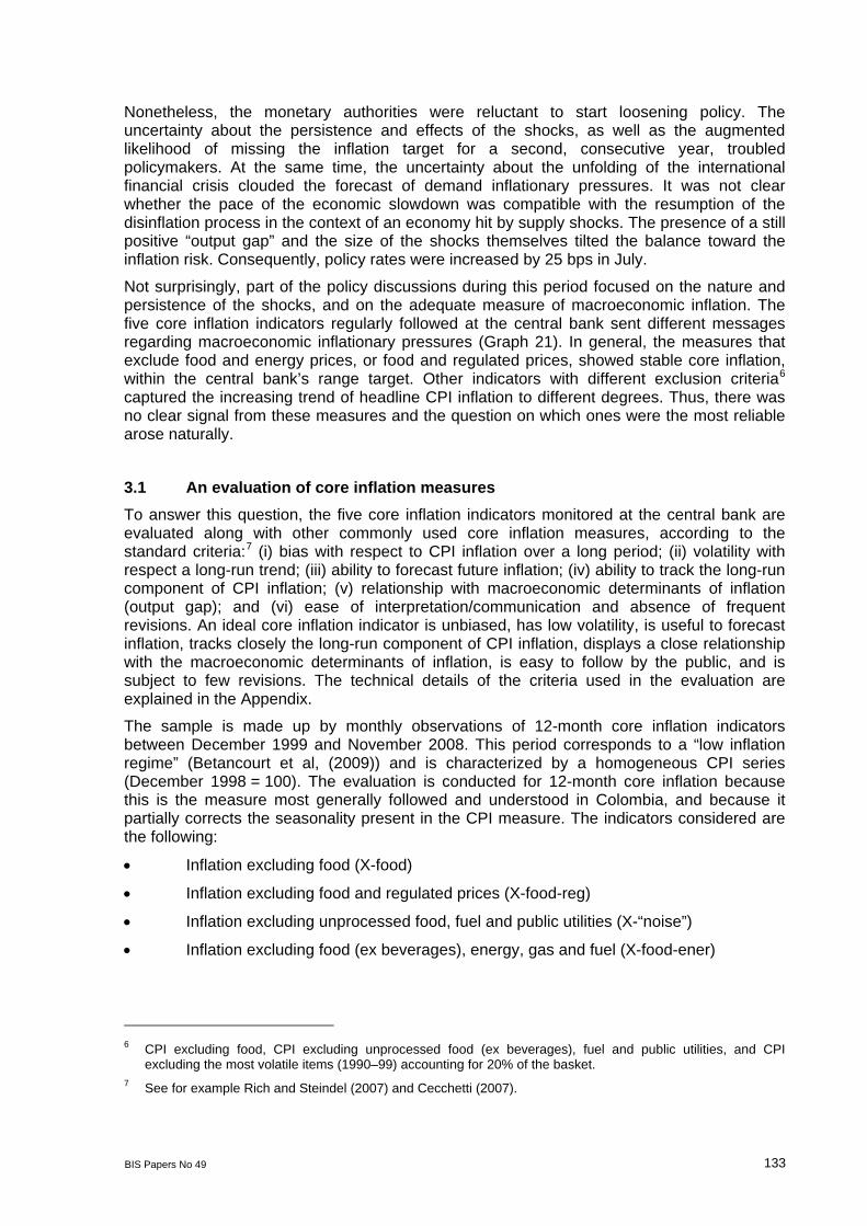
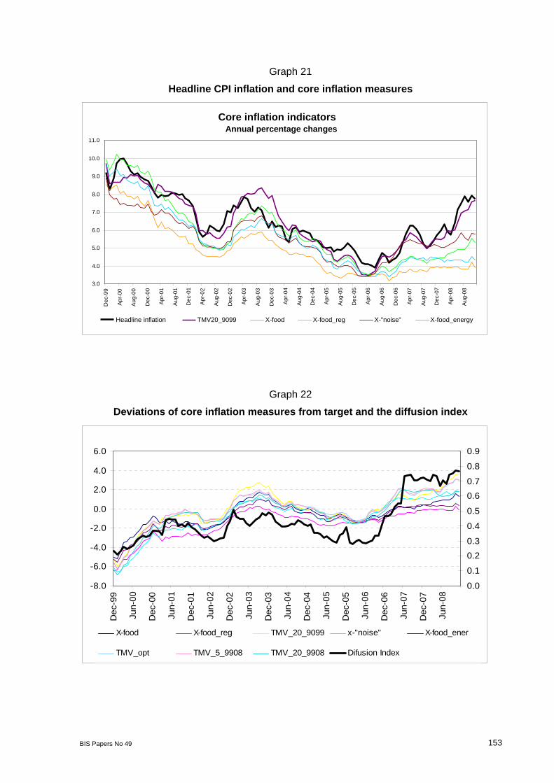
Not surprisingly, part of the policy discussions during this period focused on the nature and persistence of the shocks, and on the adequate measure of macroeconomic inflation. The five core inflation indicators regularly followed at the central bank sent different messages regarding macroeconomic inflationary pressures (Graph 21). In general, the measures that exclude food and energy prices, or food and regulated prices, showed stable core inflation, within the central bank’s range target. Other indicators with different exclusion criteria6 captured the increasing trend of headline CPI inflation to different degrees. Thus, there was no clear signal from these measures and the question on which ones were the most reliable arose naturally.
3.1 An evaluation of core inflation measures
To answer this question, the five core inflation indicators monitored at the central bank are evaluated along with other commonly used core inflation measures, according to the standard criteria:7 (i) bias with respect to CPI inflation over a long period; (ii) volatility with respect a long-run trend; (iii) ability to forecast future inflation; (iv) ability to track the long-run component of CPI inflation; (v) relationship with macroeconomic determinants of inflation (output gap); and (vi) ease of interpretation/communication and absence of frequent revisions. An ideal core inflation indicator is unbiased, has low volatility, is useful to forecast inflation, tracks closely the long-run component of CPI inflation, displays a close relationship with the macroeconomic determinants of inflation, is easy to follow by the public, and is subject to few revisions. The technical details of the criteria used in the evaluation are explained in the Appendix.
The sample is made up by monthly observations of 12-month core inflation indicators between December 1999 and November 2008. This period corresponds to a “low inflation regime” (Betancourt et al, (2009)) and is characterized by a homogeneous CPI series (December 1998 = 100). The evaluation is conducted for 12-month core inflation because this is the measure most generally followed and understood in Colombia, and because it partially corrects the seasonality present in the CPI measure. The indicators considered are the following:
Inflation excluding food (X-food)
Inflation excluding food and regulated prices (X-food-reg)
Inflation excluding unprocessed food, fuel and public utilities (X-“noise”)
Inflation excluding food (ex beverages), energy, gas and fuel (X-food-ener)
6 CPI excluding food, CPI excluding unprocessed food (ex beverages), fuel and public utilities, and CPI
excluding the most volatile items (1990–99) accounting for 20% of the basket. 7 See for example Rich and Steindel (2007) and Cecchetti (2007).

134 BIS Papers No 49
Inflation trimming the most volatile items (1990–99) accounting for 20% of the CPI basket (TMV20-9099)
Inflation trimming the most volatile items (1999–2008) accounting for 5% and 20% of the CPI basket, respectively (TMV5-9908 and TMV20-9908).
Inflation trimming the most volatile items (1999–2008), where the trimmed percentage of the basket (2.68%) was chosen to track as closely as possible the long-run component of headline CPI inflation8 (TMVop).
The median and 5%, 10% and 20% symmetric trimmed CPI inflation means.
The main results of the evaluation may be summarized as follows:
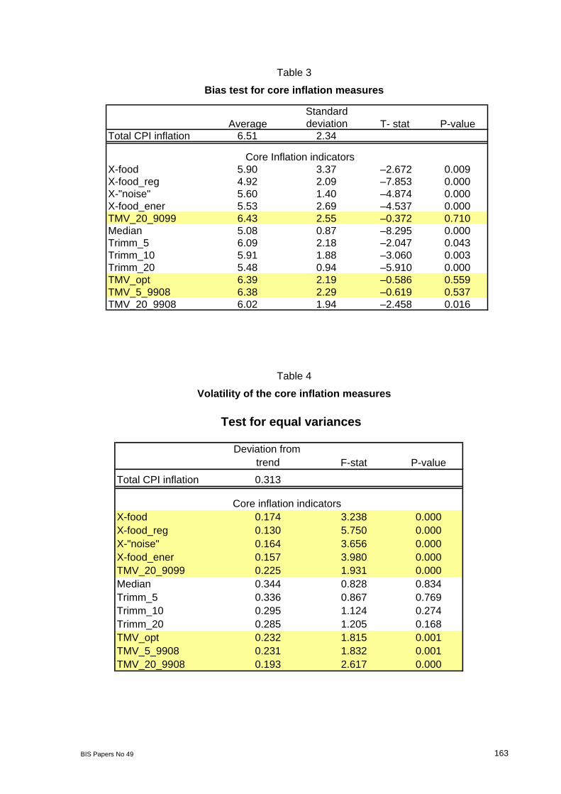
i. Bias: Table 3 shows that only the TMV indicators yield unbiased gauges of inflation. The measures that exclude food or regulated prices are generally biased downwards, a result related to the upward trend of the relative prices of these items in the sample (Graph 18).
ii. Volatility: Table 4 shows that, in general, core inflation indicators are smoother than headline CPI, with the notable exception of the median and the trimmed means.
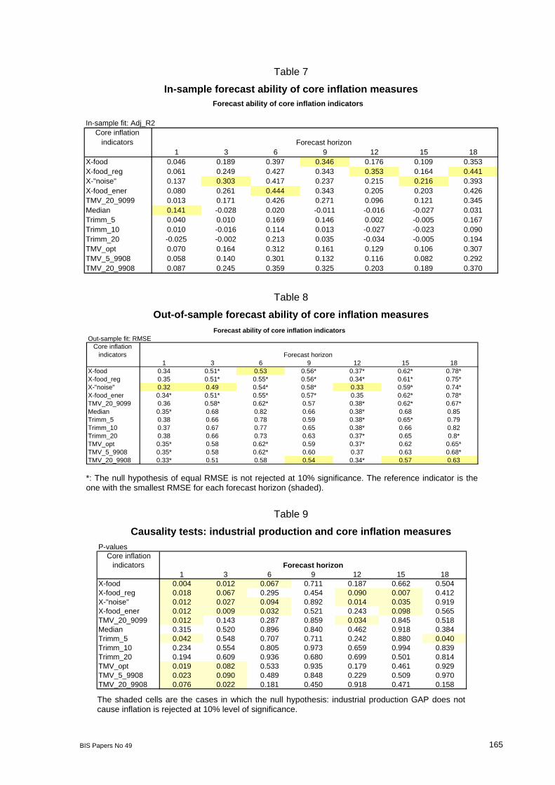
iii. Ability to forecast future headline inflation: From Table 7 it is apparent that the core measures that exclude food and some or all regulated prices help forecast future headline inflation (in-sample) better than other core inflation gauges at horizons greater than three months. Trimmed means and TMV indicators do badly in this regard. Out of sample RMSEs suggest a similar pattern, although TMV measures are now included among the indicators that better help forecast future inflation at different horizons (Table 8).
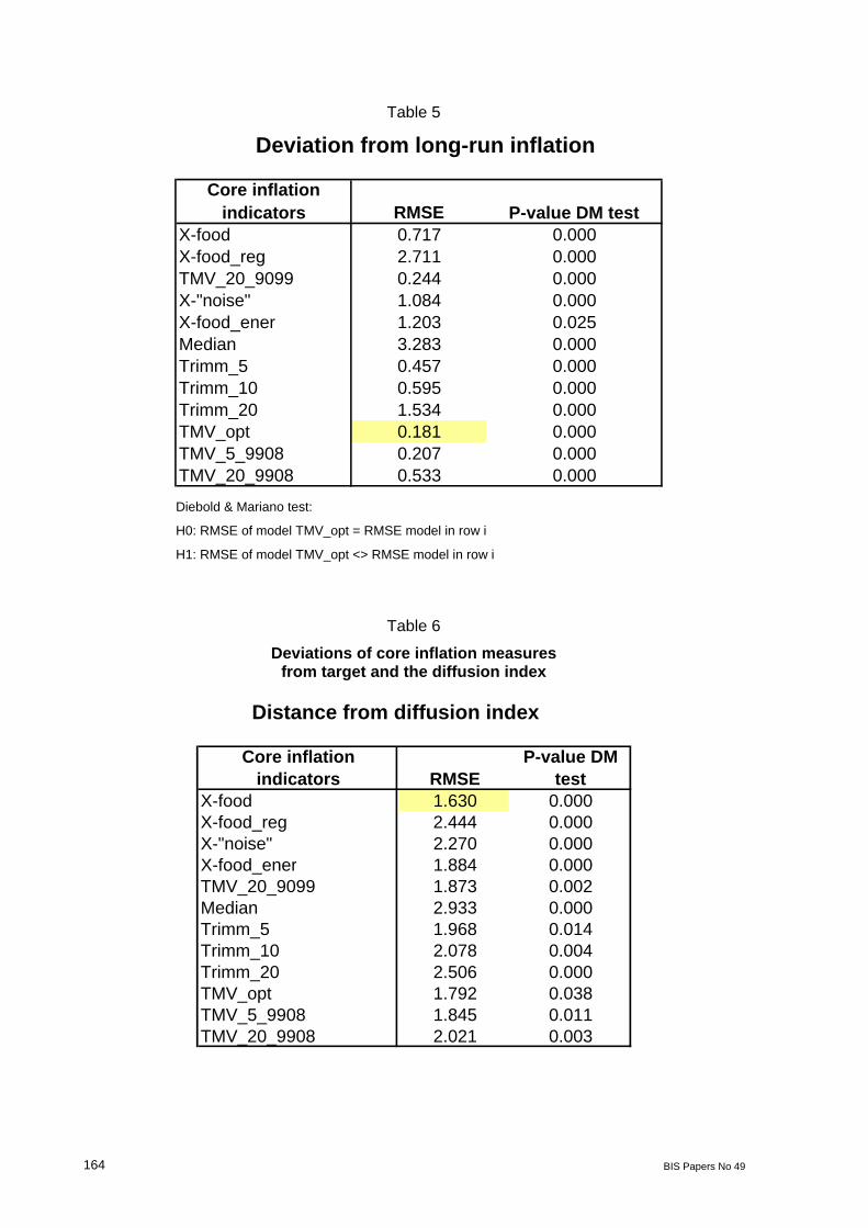
iv. Ability to track the long-run component of inflation: By construction, TMVop tracks long-run inflation best (Table 5). Other TMV measures also follow long-run inflation reasonably well, although no RMSE is significantly equal to or lower than that of TMVop according to the Diebold-Mariano test (Table 5). Measures that exclude food and some or all regulated prices fare poorly in this context, a result that is related to the bias they present.9 On the other hand, Graph 22 and Table 6 indicate that deviations of inflation without food from the inflation target closely track a diffusion index of inflationary pressures.10 The corresponding RMSE is significantly lower than that of other core inflation measures, as shown by the Diebold-Mariano test.
v. Relationship with macroeconomic determinants of inflation: Based on estimated open economy Phillips Curves,11 it follows that the industrial production output gap Granger-causes the core inflation measures that exclude food and some or all regulated prices (Table 9). There is evidence of weaker causality regarding TMV indicators and the 5% trimmed mean. In most cases, the in-sample fit of the Phillips Curves (the adjusted R2) was high (Table 10), but the best out-of-sample fit
8 The long-run component of CPI headline inflation was computed by means of a Kalman filter (see the
Appendix, section A.4) 9 If the bias were constant, these core inflation indicators could still capture turning points of “macroeconomic”
inflation. However, this does not seem to be the case for the last part of the sample (Graph 21). 10 The “diffusion index” captures the percentage of the CPI basket whose price changes are above the inflation
target. The higher the value of the diffusion index, the more widespread inflationary pressures are. In this sense, the deviation of a good core inflation indicator from the target should closely correlate with the diffusion index.
11 See the Appendix, section A.5.
BIS Papers No 49 135
was obtained for the models of inflation that exclude food and all regulated prices (Table 11). Other measures of core inflation that present good out-of-sample fit are those that exclude food and some regulated prices, as well as some of the TMV indicators.
In sum, there is no single core inflation indicator that clearly satisfies all the criteria for a good measure of core inflation. TMV indicators are unbiased and smooth, and track long-term headline inflation reasonably well. However, they are beaten by other measures at forecasting future headline inflation, and their relationship with macroeconomic determinants of inflation is weaker. Inflation excluding food and all or some regulated prices are smooth, help predict future inflation and show a stronger relationship with the output gap. Nonetheless, they are biased over the nine-year period considered and, for the same reason, fail to track the estimated long-term component of inflation, although deviations of inflation without food from the inflation targets closely followed a diffusion index of inflationary pressures.
The median and the trimmed means seem to be the poorest measures. They are biased, no less volatile than headline inflation, and do not excel in tracking long-run inflation, forecasting headline inflation, or in terms of their relationship with macro determinants. Further, they are more difficult to calculate and interpret, since the components that are excluded from the basket change frequently.
The result that no particular measure appears to be clearly superior to the others is similar to that found by Rich and Steindel (2007), who explain this as a reflection of the varying nature of the transitory shocks hitting inflation. This implies that the assessment of inflationary pressures should not rely only on one or few core inflation indicators, since some signals could be picked by some measures and not by others. More importantly, it means that the analysis of core inflation measures must be complemented with a careful examination of the persistence of the shocks and a close monitoring of their impact on inflation expectations.
For example, in Colombia conventional core inflation measures have risen moderately in the past two years, relative to other Latin American countries (BBVA (2008)) and, in the extreme case, inflation excluding food and all regulated prices has remained stable throughout the period. In a sense, this is reassuring because it provides evidence of a low pass-through of the shocks to core prices. However, it does not guarantee that macroeconomic inflation could not rise in the face of persistent increases in world commodity prices, given the lag with which they are transmitted domestically, their impact on inflation expectations and the existence of indexation mechanisms and practices. In fact, it is indicative that even as the output gap came down, non-tradable core inflation remained virtually constant in 2008 (Table 2).
3.2 The transmission of inflation shocks to core inflation and inflation expectations
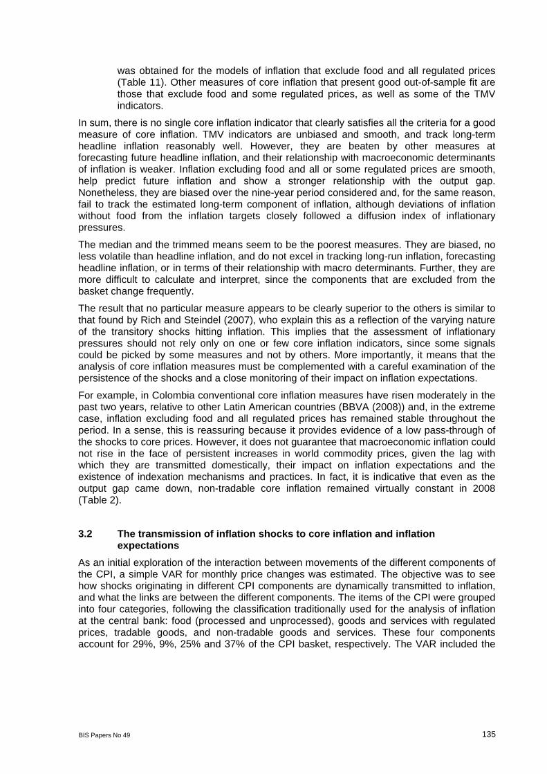
As an initial exploration of the interaction between movements of the different components of the CPI, a simple VAR for monthly price changes was estimated. The objective was to see how shocks originating in different CPI components are dynamically transmitted to inflation, and what the links are between the different components. The items of the CPI were grouped into four categories, following the classification traditionally used for the analysis of inflation at the central bank: food (processed and unprocessed), goods and services with regulated prices, tradable goods, and non-tradable goods and services. These four components account for 29%, 9%, 25% and 37% of the CPI basket, respectively. The VAR included the

136 BIS Papers No 49
monthly changes of the prices of those groups plus the change in total CPI, and was estimated for the period January 1999—November 2008.12
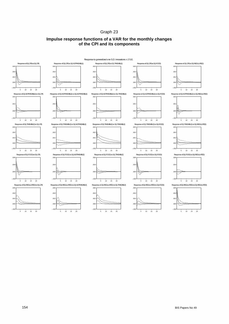
An inspection of the impulse-response functions derived from this model (Graph 23) reveals the following facts:
Food and regulated price inflation shocks are the most volatile among the components examined.
Shocks to the headline CPI monthly inflation show some persistence (two to three months), which means added persistence to annual inflation. The shocks to tradable prices have the highest persistence (eight months), and those to food prices also exhibit some persistence (two months).
A shock to headline CPI inflation has significant, positive effects on the inflation of its components. We could interpret them as responses to an innovation in macroeconomic inflation. The effect (on impact) on food prices doubles the size of the shock itself; conversely, the responses of tradable and non-tradable prices are about half the size of the shock, while the effect on regulated prices is of a similar magnitude. The responses of tradable and regulated price inflation are the most persistent. These results suggest different degrees of nominal rigidities or indexation.
The shocks to the sub-baskets of the CPI have significant, positive effects on headline monthly inflation on impact. The responses of CPI inflation to shocks to tradable and food price inflation tend to persist (up to four months). The magnitude of the response to a tradable price inflation shock (on impact) doubles the effect accounted for the size of the shock and their share of the CPI basket. The response to a shock to regulated price inflation also seems higher than the effect expected only on the basis of their share of the CPI basket.
Non-tradable price inflation does not display significant responses to shocks to tradable and food price inflation. There seems to be a significant, lagged, positive response to a regulated price inflation shock.
Tradable price inflation does not respond to a non-tradable price inflation shock. In contrast, it reacts positively in the face of food and regulated price inflation shocks, a result that may reflect the existence of a common source of the shocks (eg the exchange rate).
Food price inflation does not respond to non-tradable or regulated price inflation shocks. It responds positively to a tradable price inflation shock, again a result that may reflect the existence of a common source of the shocks (eg the exchange rate).
Regulated price inflation does not respond to a food price inflation shock. However, it reacts positively to a tradable price inflation shock and, with a lag, to a non-tradable price inflation shock.
In sum, consumer price inflation in Colombia exhibits some persistence, mostly related to the persistence of tradable and food price inflation shocks, and to the lasting responses of tradable and regulated price inflation to overall inflation shocks. Tradable and regulated price inflation shocks seem to have a relatively large impact on headline inflation. Non-tradable and tradable prices appear to be the most rigid, while food prices react strongly to overall
12 A VAR(1) was estimated. The order of the VAR was chosen according to the analysis of different information
criteria (SIC, HQ, AIC, FPE). To account for seasonality, centered dummy variables were included. A similar model has been proposed by Maureira and Leyva (2008).
BIS Papers No 49 137
inflation innovations. The transmission of shocks between the CPI components considered is rather weak, and the impacts found possibly reflect the effect of a common shock. These results suggest some diffusion of relative price or supply shocks to core inflation, but do not indicate the existence of unanchored inflation or of a fast transmission of the shocks.
There may be several explanations for these features. We will focus on indexation and the impact of the inflation shocks on inflation expectations. Indexation is a relevant factor in the transmission of supply shocks to core inflation in Colombia. First, a ruling of the Constitutional Court suggested that the purchasing power of the minimum wage should be sustained,13 which means that in practice its annual adjustment is unlikely to be lower than CPI inflation in the previous year. This is important, since the minimum wage in Colombia is relatively high and about a third of the workers in the formal sector earned it in 2006 (Arango and Posada (2007)). Furthermore, it is commonly believed that the minimum wage adjustment influences the increase in wages close the minimum. If this is true, the relevance of the minimum wage is much higher, given that 73% of the formal sector workers received less than two minimum wages in 2006 (Arango and Posada (2007)).14 Moreover, the fact that indexed contracts last for a year implies that a transitory shock may have large effects on labor costs, and that the reversion of the shock is not easily transmitted to prices. Thus, a significant channel of transmission of supply shocks to core inflation may be working through the labor cost component of several sectors in the economy.15
A second source of indexation in Colombia comes from regulated prices. In particular, the rates of electricity, gas and water/sewage are linked to past CPI or PPI. In the case of electricity and gas, the adjustments are monthly, while the changes in water/sewage prices are irregular (López, (2008)). Other regulated prices (fuel and transportation) are not automatically linked to past inflation, but are set by the regulators according to the evolution of costs.16 Interestingly, López (2008) found that regulated price inflation is less persistent than overall inflation, and specifically, less persistent than services price inflation, a result that draws attention back to wage indexation. In addition to wage and regulated price indexation, there are other informal indexation practices that may help explain why inflation persistence remains high in Colombia, despite a reduction after the fall of inflation and the adoption of an inflation targeting regime (Vargas, 2007).
In addition to indexation, the credibility of monetary policy may determine the extent to which supply shocks are transmitted to core inflation. González and Hamann (2006) argue that the high degree of persistence of inflation in Colombia has to do with imperfect credibility. The latter in turn is associated with the fact that the long-run inflation target has not been reached, which implies a slow process of learning about the “permanent” component of the inflation target. Indeed, the evidence presented in Gómez and Hamann (2006) favors this explanation over a simple ad hoc indexation hypothesis. Thus, an examination of the determinants of inflation expectations is warranted.
13 Corte Constitucional del Colombia, Sentencia (ruling) C-815/99. 14 Nevertheless, Arango and Posada (2006) found that there is no long-run (co-integration) relationship between
the real minimum wage and a real private sector wage obtained from household surveys. According to these authors, the correlation coefficient between changes of the real minimum wage and the real private sector wage was just 0.252 between 1984 and 2005. On the other hand, negotiations between trade unions and firms that result in labor contracts with wage increases for more than one year usually index the second or third year increases to observed CPI inflation. However, the fraction of the labor force covered by such contracts is very low.
15 The minimum wage is also used to index fines and some pensions. 16 In the case of fuel, the determination of the producer and consumer prices is rather complex, since it involves
taxes and subsidies at different government levels (Rincón (2008)).
138 BIS Papers No 49
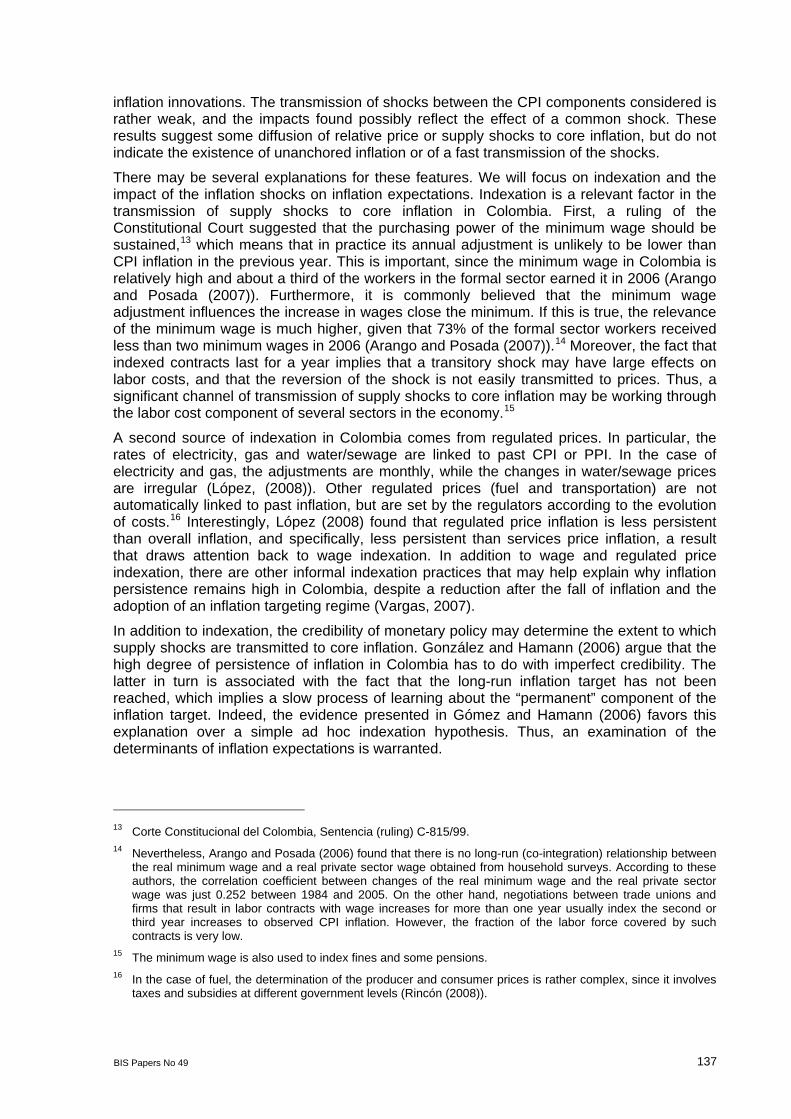
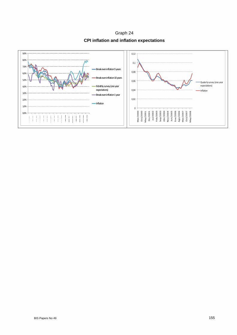
In Colombia the central bank conducts two surveys of inflation expectations: a monthly survey (since 2003) directed mostly to financial and banking sector analysts, and a quarterly survey (since 2000) with a broader coverage (businessmen, unions and academia among others). Furthermore, break-even inflation expectations implicit in the public debt market have been constructed since 2003. Monthly survey and break-even annual inflation expectations seem to be unbiased (with respect to future inflation) for the period without the large relative price shocks (2001–06, Table 12). In contrast, quarterly survey annual inflation expectations tend to exceed future inflation for the same time-span (Table 12). As expected, there are great forecast errors in the years of the relative price shocks (2007–08, Table 12). All inflation expectations indicators were as volatile as headline inflation throughout the 2000–08 sample, a feature that may be interpreted as evidence of imperfect credibility of monetary policy (imperfect anchoring of inflation expectations) during this period (Table 13).
However, Graph 24 shows that annual/annualized inflation expectations have not increased as much as inflation after the recent supply shocks. In the case of one-year-ahead 12-month inflation expectations, this means that the shocks were perceived as transitory (though persistent) events and that the credibility of monetary policy (the inflation target) may be playing a role. However, the fact that the five- and 10-year break-even inflation expectations rose by almost 200 bps imply that longer-term inflation expectations are far from being anchored.17 Below, two questions regarding the determination of inflation expectations are given a preliminary answer: (i) how are inflation expectations formed? And, in particular, what is the role of past inflation and the inflation targets? (ii) how do inflation expectations respond to supply shocks?
i. The formation of inflation expectations: In order to explore what the impact of inflation and the inflation target on inflation expectations is, two reduced form equations for the inflation expectations were estimated. The models were fitted to the data coming from the monthly and quarterly surveys described earlier.18
12413,
11,121,
12, tm
tmme
ttme
tt 443
,3,121
,4, t
qt
qqett
qett
ett 12, and e
tt 4, represent the one-year-ahead 12-month inflation expectations
obtained in period t from the monthly and quarterly surveys, respectively; mett
,11,1
and qett
,3,1 represent one lag autoregressive term, 1t
m and tq represent the
relevant inflation rate observed when the respective survey is collected and 12tm
and 4tq represent the inflation target set by the central bank. The superscripts m
and q indicate the monthly and quarterly frequency of the data. The following are the results of the estimation.19
17 This conclusion must be qualified though, since the inflation risk premia may be experiencing large
movements. 18 The timing of the monthly survey is as follows: At time t, when respondents report their 12-month inflation
expectations for t+12 ( mett,
12, ), they have not observed current annual inflation ( tm ), but they had observed
inflation in t–1 ( 1tm ). That is why current inflation is excluded from the regression and the one period
lagged inflation is the “relevant” variable to analyze the impact of past inflation on expectations. In the case of the quarterly survey, the respondent observes annual inflation of quarter t before he/she projects annual inflation one year (four quarters, t+4 periods) ahead. That is why annual inflation in t is the “relevant” measure to capture the effect of past inflation on expectations.
19 For both estimated equations, residuals have a normal distribution and do not display serial correlation.
BIS Papers No 49 139
Equation Results (p-values in parentheses)
Estimated equation for monthly data
12)007.0(
1)000.0(
,11,1)065.0()579.0(
,12, 47.017.034.00.0 t
mt
mmett
mett
Estimated equation for quarterly data
4)057.0()009.0(
,3,1)000.0()810.0(
,4, 29.037.036.00.0 t
qt
qqett
qett
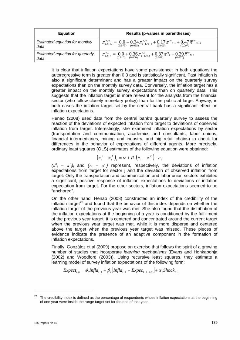
It is clear that inflation expectations have some persistence: in both equations the autoregressive term is greater than 0.3 and is statistically significant. Past inflation is also a significant determinant and has a greater impact on the quarterly survey expectations than on the monthly survey data. Conversely, the inflation target has a greater impact on the monthly survey expectations than on quarterly data. This suggests that the inflation target is more relevant for the analysts from the financial sector (who follow closely monetary policy) than for the public at large. Anyway, in both cases the inflation target set by the central bank has a significant effect on inflation expectations.
Henao (2008) used data from the central bank’s quarterly survey to assess the reaction of the deviations of expected inflation from target to deviations of observed inflation from target. Interestingly, she examined inflation expectations by sector (transportation and communication, academics and consultants, labor unions, financial intermediaries, mining and industry, and big retail chains) to check for differences in the behavior of expectations of different agents. More precisely, ordinary least squares (OLS) estimates of the following equation were obtained:
tTttjj
Tt
et
(et – T
t)j and (t – Tt) represent, respectively, the deviations of inflation
expectations from target for sector j and the deviation of observed inflation from target. Only the transportation and communication and labor union sectors exhibited a significant, positive response of inflation expectations to deviations of inflation expectation from target. For the other sectors, inflation expectations seemed to be “anchored”.
On the other hand, Henao (2008) constructed an index of the credibility of the inflation target20 and found that the behavior of this index depends on whether the inflation target of the previous year was met. She also found that the distribution of the inflation expectations at the beginning of a year is conditioned by the fulfillment of the previous year target: it is centered and concentrated around the current target when the previous year target was met, while it is more disperse and centered above the target when the previous year target was missed. These pieces of evidence indicate the presence of an adaptive component in the formation of inflation expectations.
Finally, González et al (2009) propose an exercise that follows the spirit of a growing number of studies that incorporate learning mechanisms (Evans and Honkapohja (2002) and Woodford (2003)). Using recursive least squares, they estimate a learning model of survey inflation expectations of the following form:
20 The credibility index is defined as the percentage of respondents whose inflation expectations at the beginning
of one year were inside the range target set for the end of that year.
1,111, tthhtttttht ShockExpecInflaInflaExpect
140 BIS Papers No 49
where htExpect , represents the inflation expectations at time t for horizon h, 1tInfla
represents the corresponding lagged inflation rate hExpecInfla htt ,11
corresponds to a forecasting error that reflects the learning process and 1tShock
represents unexpected monetary policy shocks.21 They found that the largest parameter estimate was t , which happened to be relatively constant and close to
1, reflecting the important impact that observed inflation has on expectations. The learning parameter, t , and the parameter that reflects the unanticipated policy
shock, t , were relatively small, suggesting a slow learning rate.
Based on the previous evidence, it is clear that survey inflation expectations are strongly affected by past inflation, so that persistent “supply” or “demand” shocks may have long-lasting effects on core inflation, if price/wage formation is influenced by these expectations. However, there is also evidence of an impact of the inflation targets on survey inflation expectations and of some anchoring of the expectations of some sectors of the economy. Hence, shocks are not fully transmitted and monetary policy credibility seems to play a relevant role.
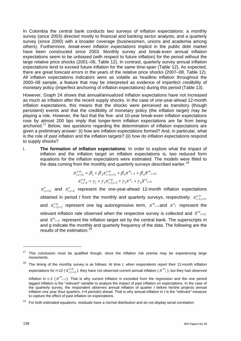
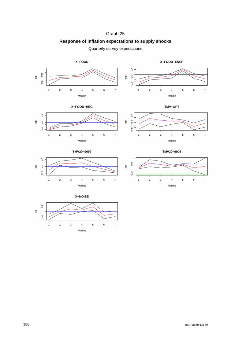
ii. The response of inflation expectations to supply shocks: To assess the response of inflation expectations to supply shocks, two empirical exercises were carried out. First, estimates of the supply shocks were computed as the difference between annual CPI headline inflation and several measures of core inflation.22 The deviations of inflation expectations (obtained from surveys or break-even inflation) from headline inflation were then regressed against the estimated supply shocks in order to gauge the response of expectations to the shocks:
t
p
kkt
ektij
ctt
hijht
eht
iji
1
for core inflation indicator j and inflation expectations i at horizon t+h. ij0 measures
the contemporaneous effect of a supply shock on the deviations of inflation expectations with respect to inflation. The value of this parameter can be associated with the credibility of the inflation regime. For instance, if ij
0 equals –1, then a transitory supply shock does not affect expectations, implying a perfectly credible monetary regime. On the contrary, if ij
0 equals 0, then a transitory supply shock affects inflation expectations as much as it affects inflation itself.
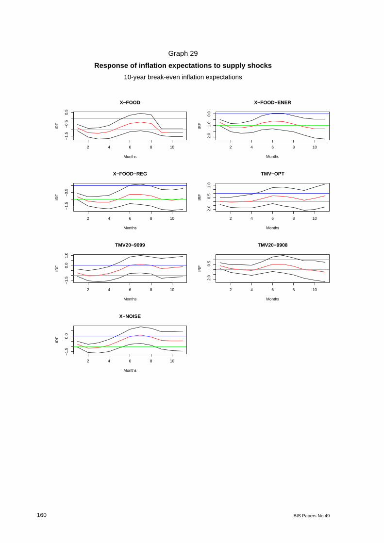
Since a supply shock is likely to have persistent effects, we estimated ijh for a set of
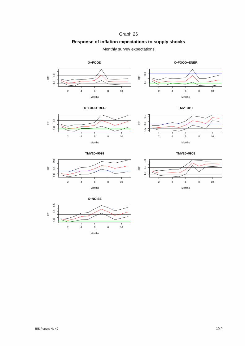
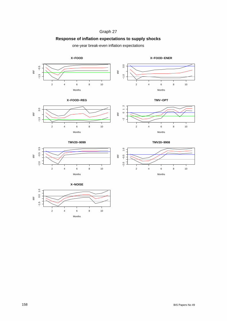
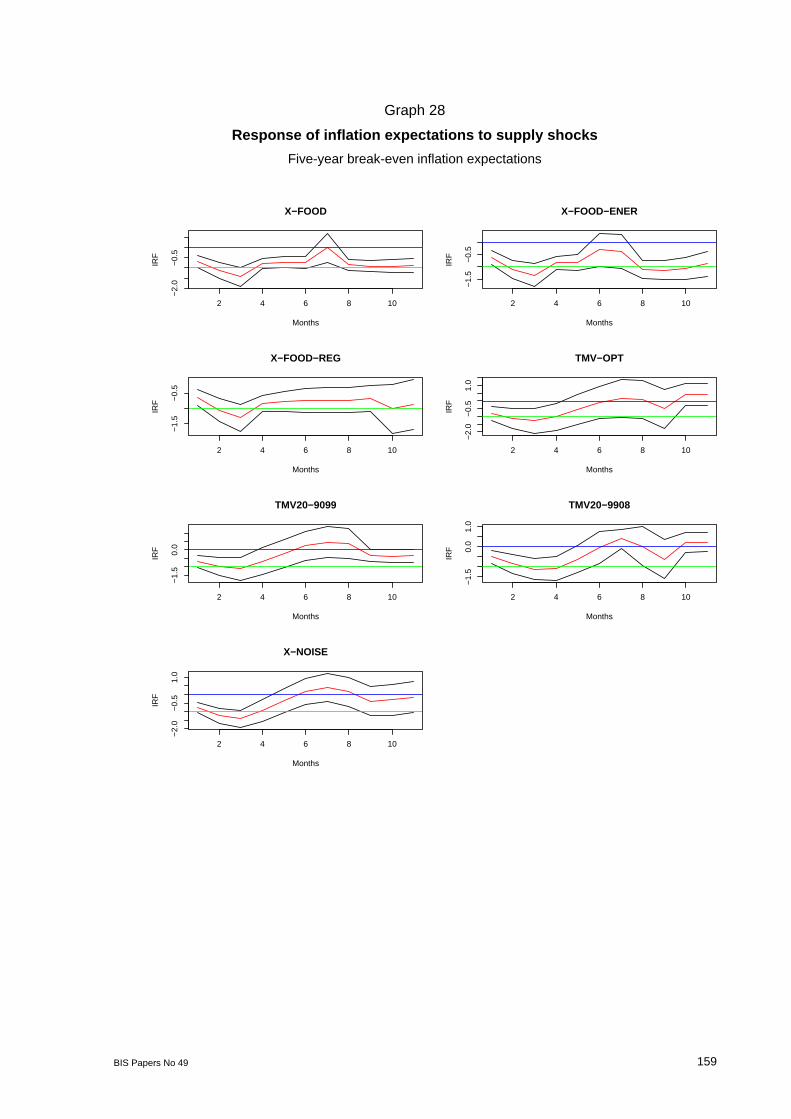
regressions where the dependent variable is leading the independent variable by h periods. That is, Graphs 25 to 29 present the sequence of ij
h for several values of h. In general, one can see from the graphs that inflation expectations are partially anchored and that supply shocks do not affect one-to-one inflation expectations. In fact, for most of the cases the estimated impact was negative, though greater than –1, ie transitory supply shocks are not entirely transmitted to inflation expectations, but there is no evidence of a perfectly credible regime.
There are some drawbacks to this approach, since the estimated equation is a reduced form of a system that may involve both demand and supply shocks with
21 These shocks were constructed as the difference between actual and expected policy interest rates, where
the latter were obtained from a Bloomberg survey. 22 See Section 3.1
BIS Papers No 49 141
different degrees persistence, hitting the economy under varying monetary policy credibility. Hence, the estimates may be biased for several reasons.23
In a second exercise we measured the impact of inflation “surprises” on the dynamics of quarterly survey inflation expectations. The objective was to estimate the extent to which inflation expectations are adjusted following an inflation surprise. More precisely:
tttiitt SA 1|
where:
ttttt
ittittitt
ES
EEA
11
1|
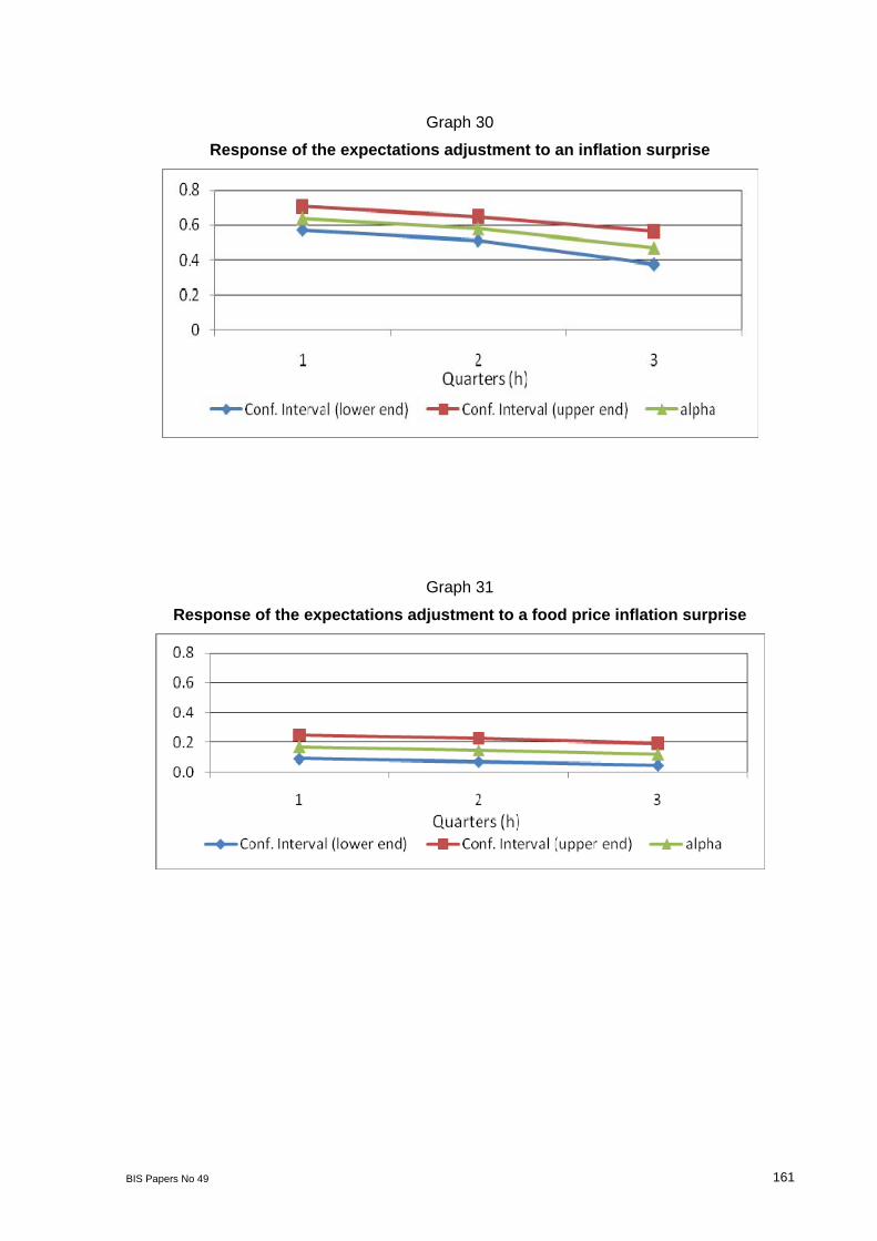
At|t+i represents the adjustment of the inflation expectations (at a fixed horizon) and St
t–1 proxies the inflation surprises. The coefficient i gauges the impact of the latter on the expectations adjustment. If expectations were not anchored, a transitory inflation surprise would be totally transmitted to the expectations (i close to one). The results of the estimation are presented in Graph 30. It is clear that the impact of inflation surprises on the expectation adjustment is significantly positive, less than one and decreasing with the expectation horizon. This can be interpreted as evidence of partial and declining transmission of inflation surprises to expectations. However, to obtain more robust results and reduce the probability of bias, this exercise could be improved to distinguish between demand and supply shocks, or persistent and short-lived shocks.
In another version of this exercise, the inflation surprise was redefined as:
ttat
tt ES 11
that is, as the difference between food price inflation and the past expectation of current inflation. To eliminate predictable, low frequency movements of the relative price of food, the deviations of St
t–1 with respect to its long-run trend (Hodrick-Prescott) were used in the estimation. The idea was to identify the effects of short-lived supply shocks, as approximated by short-run food price movements. Graph 31 indicates again a positive impact of the shocks on the expectations adjustment, but of significantly lower magnitude.
4. Conclusion
The assessment of inflationary pressures in Colombia has faced two important challenges in the present decade. The first occurred in 2006 and consisted of detecting an overheating economy in the midst of fast-growing investment and increasing measured productivity. These phenomena suggested a large, possibly permanent supply shock that did not imply a risk to the achievement of the inflation target. In fact, at the time inflation reached a historical minimum. However, the central bank raised the policy interest rates anticipating a strong
23 One that is particularly important for the purpose of this paper is a situation in which monetary policy is not
fully credible, inflation falls faster than expected inflation, following a permanent demand shock, but the economy is also hit by a myriad of supply shocks. In this case, a negative value of beta may emerge that does not imply a credible monetary policy regime. Nonetheless, an inspection of the scatter plots indicates that this situation has low probability, since significant portions of the data are located in an area that clearly suggests the presence of credibility in the sample.

142 BIS Papers No 49
demand pressure on the basis of other indicators, a decision that proved to be timely. Traditional indicators of productivity and unit labor costs were not sufficient to identify “supply” and “demand” movements, so the policymakers had to rely on a wider array of variables to gauge the state of the economy.
The second challenge took place in 2007–08, when the economy was hit by a number of supply shocks and core inflation indicators sent diverging signals about the transmission of those shocks to macroeconomic inflation. An evaluation of the core inflation indicators according to standard criteria suggests that no particular measure seems to be clearly superior to the others, a result similar to that found by Rich and Steindel (2007), who explain this as a reflection of the varying nature of the transitory shocks hitting inflation. This implies that the assessment of inflationary pressures should not rely only on a single or few core inflation indicators, since some signals could be picked by some measures and not by others. More importantly, it means that the analysis of core inflation measures must be complemented with a careful examination of the persistence of the shocks and a close monitoring of their impact on inflation expectations. In fact, core inflation measures are used to derive estimates of the supply shocks hitting the economy to assess their impact on inflation expectations. It was found that the latter are formed on the basis of past inflation, but that the inflation target also plays a role. Moreover, inflation expectations partially move with supply shocks, an outcome that reflects a degree of credibility of monetary policy.
BIS Papers No 49 143
Graph 1
Real exchange rate
Real exchange rate index (deflated by CPI)
60
80
100
120
140
160
Nov-98 Nov-99 Nov-00 Nov-01 Nov-02 Nov-03 Nov-04 Nov-05 Nov-06 Nov-07 Nov-08
Graph 2
Aggregate domestic demand and GDP real growth
-2
0
2
4
6
8
10
12
14
Mar
-01
Sep-
01
Mar
-02
Sep-
02
Mar
-03
Sep-
03
Mar
-04
Sep-
04
Mar
-05
Sep-
05
Mar
-06
Sep-
06
Mar
-07
Sep-
07
Mar
-08
Sep-
08Annual GDP and Final Domestic Demand Growth
GDP Final Domestic Demand
144 BIS Papers No 49
Graph 3
CPI inflation and targets
Graph 4
Output gap
Colombian output gap1998–2008
–6%
–4%
–2%
0%
2%
4%
Mar
-98
Mar
-99
Mar
-00
Mar
-01
Mar
-02
Mar
-03
Mar
-04
Mar
-05
Mar
-06
Mar
-07
Mar
-08
BIS Papers No 49 145
Graph 5
Investment ratio
Graph 6
Growth of the capital stock
Source: DPI, Banco de la República
Gross fixed investment/GDP(Base 2000)
0.00
5.00
10.00
15.00
20.00
25.00
30.00
Mar
-77
Dec
-77
Sep-
78
Jun-
79
Mar
-80
Dec
-80
Sep-
81
Jun-
82
Mar
-83
Dec
-83
Sep-
84
Jun-
85
Mar
-86
Dec
-86
Sep-
87Ju
n-88
Mar
-89
Dec
-89
Sep-
90
Jun-
91
Mar
-92
Dec
-92
Sep-
93
Jun-
94
Mar
-95
Dec
-95
Sep-
96
Jun-
97M
ar-9
8
Dec
-98
Sep-
99
Jun-
00
Mar
-01
Dec
-01
Sep-
02
Jun-
03
Mar
-04
Dec
-04
Sep-
05
Jun-
06
Mar
-07
Dec
-07
Growth of the capital stock
0.0%
1.0%
2.0%
3.0%
4.0%
5.0%
6.0%
7.0%
8.0%
9.0%
1982
1983
1984
1985
1986
1987
1988
1989
1990
1991
1992
1993
1994
1995
1996
1997
1998
1999
2000
2001
2002
2003
2004
2005
2006
2007
2008
146 BIS Papers No 49
Graph 7
Growth of Solow residual
Source: DPI, Banco de la República
Graph 8
Real and nominal policy interest rates
Growth of Solow residual
–10.00%
–8.00%
–6.00%
–4.00%
–2.00%
0.00%
2.00%
4.00%
1982
1983
1984
1985
1986
1987
1988
1989
1990
1991
1992
1993
1994
1995
1996
1997
1998
1999
2000
2001
2002
2003
2004
2005
2006
2007
2008
BIS Papers No 49 147
Graph 9
Total factor productivity and labor productivity
Y/L = GDP/adjusted employment A = Solow residual See footnote 1
Source: DPI, Banco de la República
Graph 10
TFP and TFP trend
Source: DPI, Banco de la República
TFP and labor productivity
4.7
4.8
4.9
5 5.1
5.2
5.3
5.4
5.5
5.6
5.7
5.8
2000 2001 2002 2003 2004 2005 2006 2007 2008
Y/L
2.15
2.20
2.25
2.30
2.35
2.40
2.45
2.50
2.55
A Y/L
A
Solow residual
2.15
2.20
2.25
2.30
2.35
2.40
2.45
2.50
2.55
1981
1982
1983
1984
1985
1986
1987
1988
1989
1990
1991
1992
1993
1994
1995
1996
1997
1998
1999
2000
2001
2002
2003
2004
2005
2006
2007
2008
Solow residual Filtered Solow residual
148 BIS Papers No 49
Graph 11
Labor productivity in the manufacturing industry
Output per worker
Source: DANE, calculations from DPI, Banco de la República
Graph 12
Labor productivity in the manufacturing industry
Output per hour
Source: DANE, calculations from DPI, Banco de la República
Output per worker
50
70
90
110
130
150
170
190
210
230
Jan-80 Aug-81 Mar-83 Oct-84 May-86 Dec-87 Jul-89 Feb-91 Sep-92 Apr-94 Nov-95 Jun-97 Jan-99 Aug-00 Mar-02 Oct-03 May-05 Dec-06 Jul-08 Output per worker
Filtered output per worker
Output per hour
0.7
0.8
0.9
1
1.1
1.2
1.3
1.4
1.5
1.6
Jan-90
Dec-90
Nov-91
Oct-92
Sep-93
Aug-94
Jul-95
Jun-96
May-97
Apr-98
Mar-99
Feb-00
Jan-01
Dec-01
Nov-02
Oct-03
Sep-04
Aug-05
Jul-06
Jun-07
May- 08
Ouput per hour Filtered output per hour
BIS Papers No 49 149
Graph 13
Unit labor costs for the manufacturing industry
Nominal ULC for the Manufacturing Industry (Change YoY)
-10%
-5%
0%
5%
10%
15%
20%
Oct
-00
Abr
-01
Oct
-01
Abr
-02
Oct
-02
Abr
-03
Oct
-03
Abr
-04
Oct
-04
Abr
-05
Oct
-05
Abr
-06
Oct
-06
Abr
-07
Oct
-07
Abr
-08
Oct
-08
Source: DANE-MMM
Per hour Per worker
Source: DANE, calculations from DPI, Banco de la República
Graph 14
Unit labor costs for retail industry
Nominal ULC for the Retail Industry(Change YoY)
-10%
-5%
0%
5%
10%
15%
20%
Oct
-00
Abr
-01
Oct
-01
Abr
-02
Oct
-02
Abr
-03
Oct
-03
Abr
-04
Oct
-04
Abr
-05
Oct
-05
Abr
-06
Oct
-06
Abr
-07
Oct
-07
Abr
-08
Oct
-08
So urce: DANE-MMM
Source: DANE, calculations from DPI, Banco de la República
150 BIS Papers No 49
Graph 15
Capacity utilization indices for the manufacturing industry
DANE-ANDI
Source: DANE and Fedesarrollo
Graph 16
Consumer confidence indicator and consumption growth
0
5
10
15
20
25
30
35
0
1
2
3
4
5
6
7
8
9
10
20
03
Q3
20
03
Q4
20
04
Q1
20
04
Q2
20
04
Q3
20
04
Q4
20
05
Q1
20
05
Q2
20
05
Q3
20
05
Q4
20
06
Q1
20
06
Q2
20
06
Q3
20
06
Q4
20
07
Q1
20
07
Q2
20
07
Q3
20
07
Q4
20
08
Q1
20
08
Q2
20
08
Q3
*Ave
rag
e O
ct …
Ave
rag
e In
de
x of th
e F
ed
esa
rrollo
con
sum
ptio
n
Ind
icato
rs
An
nu
al G
row
th o
f Ho
ush
old
Co
nsu
mp
tion
Source: Fedesarrollo. Calculations Banco de la República* Average of ICC, IEC and ICE; Consumer Confidence Index, Consumption expectation index and Economic Conditions Index, respectively.
Consumption Confidence Indicator and Household Consumption
Household Consumption
Average of Fedesarrollo's Index*
Capacity utilization indices for the manufacturing industry
60.0
65.0
70.0
75.0
80.0
85.0
Mar
-98
Sep-
98
Mar
-99
Sep-
99
Mar
-00
Sep-
00
Mar
-01
Sep-
01
Mar
-02
Sep-
02
Mar
-03
Sep-
03
Mar
-04
Sep-
04
Mar
-05
Sep-
05
Mar
-06
Sep-
06
Mar
-07
Sep-
07
Mar
-08
Sep-
08
ANDI FEDESARROLLO
BIS Papers No 49 151
Graph 17
Real credit growth
Graph 18
Relative food and regulated prices*
*CPI regulated and food prices / Headline CPI
Relative prices
95
105
115
125
135
145
155
Jan-
99
Jan-
00
Jan-
01
Jan-
02
Jan-
03
Jan-
04
Jan-
05
Jan-
06
Jan-
07
Jan-
08
95
100
105
110
115
Regulated (left axis) Food (right axis)
Real credit growth
–20.0%
–10.0%
0.0%
10.0%
20.0%
30.0%
No
v-00
No
v-01
No
v-02
No
v-03
No
v-04
No
v-05
No
v-06
No
v-07
No
v-08
Yea
r o
n y
ear
chan
ge
152 BIS Papers No 49
Graph 19
PPI inflation and the nominal depreciation of the COP
Graph 20
Impact of price shocks on real disposable income
PPI inflation and nominal depreciation(change yoy)
–30%
–25%
–20%
–15%
–10%
–5%
0%
5%
10%
15%
20%
Jan-06 May-06 Sep-06 Jan-07 May-07 Sep-07 Jan-08 May-08 Sep-08 –4%
–2%
0%
2%
4%
6%
8%
10%
12%
14%
Nominal depreciation PPI inflation
Real minimum wage(% change yoy, deflated with headline CPI)
–2.0%
–1.5%
–1.0%
–0.5%
0.0%
0.5%
1.0%
1.5%
2.0%
2.5%
3.0%
3.5%
Dec
-00
Apr
-01
Aug
-01
Dec
-01
Apr
-02
Aug
-02
Dec
-02
Apr
-03
Aug
-03
Dec
-03
Apr
-04
Aug
-04
Dec
-04
Apr
-05
Aug
-05
Dec
-05
Apr
-06
Aug
-06
Dec
-06
Apr
-07
Aug
-07
Dec
-07
Apr
-08
Aug
-08
Dec
-08
BIS Papers No 49 153
Graph 21
Headline CPI inflation and core inflation measures
Graph 22
Deviations of core inflation measures from target and the diffusion index
-8.0
-6.0
-4.0
-2.0
0.0
2.0
4.0
6.0
De
c-9
9
Jun
-00
De
c-0
0
Jun
-01
De
c-0
1
Jun
-02
De
c-0
2
Jun
-03
De
c-0
3
Jun
-04
De
c-0
4
Jun
-05
De
c-0
5
Jun
-06
De
c-0
6
Jun
-07
De
c-0
7
Jun
-08
0.0
0.1
0.2
0.3
0.4
0.5
0.6
0.7
0.8
0.9
X-food X-food_reg TMV_20_9099 x-"noise" X-food_ener
TMV_opt TMV_5_9908 TMV_20_9908 Difusion Index
Core inflation indicatorsAnnual percentage changes
3.0
4.0
5.0
6.0
7.0
8.0
9.0
10.0
11.0
De
c-9
9
Ap
r-0
0
Au
g-0
0
De
c-0
0
Ap
r-0
1
Au
g-0
1
De
c-0
1
Ap
r-0
2
Au
g-0
2
De
c-0
2
Ap
r-0
3
Au
g-0
3
De
c-0
3
Ap
r-0
4
Au
g-0
4
De
c-0
4
Ap
r-0
5
Au
g-0
5
De
c-0
5
Ap
r-0
6
Au
g-0
6
De
c-0
6
Ap
r-0
7
Au
g-0
7
De
c-0
7
Ap
r-0
8
Au
g-0
8
Headline inflation TMV20_9099 X-food X-food_reg X-"noise" X-food_energy
154 BIS Papers No 49
Graph 23
Impulse response functions of a VAR for the monthly changes of the CPI and its components
–.001
.000
.001
.002
.003
5 10 15 20
R e s p o n se o f
D (LC P I)
to D (L C P I)
–.001
.000
.001
.002
.003
5 10 15 20
R e s p o n s e o f D ( L C PI)
to
D ( L N OTR A D A B L E )
–.001
.000
.001
.002
.003
5 10 15 20
Response of
D(LCPI)
to
D(LTRADABLE)
–.001
.000
.001
.002
.003
5 10 15 20
Response of
D(LCPI)
to
D(LFOOD)
–.001 .000
.001
.002
.003
5 10 15 20
R e s p o n s e o f D ( L C P I ) to
D(LREGULATED)
–.001
.000
.001
.002
5 10 15 20
R e s p o n s e o f D (L N O TR A D A B L E )
to
D (L C P I )
–.001
.000
.001
.002
5 10 15 20
R e s p o n s e of
D (L N O TR ADABL E ) to D ( L N OTR A D A B L E )
–.001
.000
.001
.002
5 10 15 20
R e sponse of
D(LNOTRADABLE)
to
D(LTRADABLE)
–.001
.000
.001
.002
5 10 15 20
Response of
D(LNOTRADABLE)
to
D(LFOOD )
–.001
.000
.001
.002
5 10 15 20
R e s p o n s e o f
D ( L N O TR A DABLE) to
D(LREGULATED)
–.001
.000
.001
.002
.003
5 10 15 20
R e s p o ns e o f D (L TR A D A B LE )
t o
D ( L C P I )
–.001
.000
.001
.002
.003
5 10 15 20
R e sp o n se o f D ( L TR A DABLE)
to D ( L N OTR A D A B L E )
–.001
.000
.001
.002
.003
5 10 15 20
R esponse of
D(LTRADABLE)
to
D(LTRADABLE)
–.001
.000
.001
.002
.003
5 10 15 20
Response of
D(LTRADABLE)
to
D(LFOOD )
–.001 .000
.001
.002
.003
5 10 15 20
R e s p o n se o f
D ( L TR A D ABLE)
to
D(LREGULATED)
–.004
.000
.004
.008
5 10 15 20
R es po ns e o f
D ( L F O O D ) t o D ( L C P I)
–.004
.000
.004
.008
5 10 15 20
R es po n s e of
D ( L FOOD) to
D ( LN OTR A D A B L E )
–.004
.000
.004
.008
5 10 15 20
Response of
D(LFOOD)
to
D(LTRADABLE)
–.004
.000
.004
.008
5 10 15 20
Response of
D(LFOOD)
to
D(LFOOD)
–.004
.000
.004
.008
5 10 15 20
R e s p o n s e o f
D ( L FOOD)
to
D(LREGULATED)
–.002
.000
.002
.004
.006
5 10 15 20
R e sp o n s e of
D (L R E GU L A TE D ) t o D ( L C P I)
–.002
.000
.002
.004
.006
5 10 15 20
R e s p o n s e of
D (L R E GU LATED ) to D ( L N OTR A D A B L E )
–.002
.000
.002
.004
.006
5 10 15 20
R e sponse of
D(LREGULATED)
to
D(LTRADABLE)
–.002
.000
.002
.004
.006
5 10 15 20
Response of
D(LREGULATED)
to
D(LFOOD )
–.002 .000
.002
.004
.006
5 10 15 20
R e s p o n s e o f D (L R E GU L ATED)
to
D(LREGULATED)
R es pons e t o
generalized one
S.D.
innovations
± 2 S.E.
BIS Papers No 49 155
Graph 24
CPI inflation and inflation expectations
0,0%
1,0%
2,0%
3,0%
4,0%
5,0%
6,0%
7,0%
8,0%
9,0%
May-03
Sep-03
Ene-04
May-04
Sep-04
Ene-05
May-05
Sep-05
Ene-06
May-06
Sep-06
Ene-07
May-07
Sep-07
Ene-08
May-08
Sep-08
Break even inflation 5 years
Break even inflation 10 years
Monthly survey (one year expectations)
Break even inflation 1 year
Inflation
0
0,02
0,04
0,06
0,08
0,1
0,12
Ma
r/2
00
0
Oc
t/2
00
0
Ma
y/2
00
1
Dic
/20
01
Jul/
20
02
Fe
b/2
00
3
Se
p/2
00
3
Ab
r/2
00
4
No
v/2
00
4
Jun
/20
05
En
e/2
00
6
Ag
o/2
00
6
Ma
r/2
00
7
Oc
t/2
00
7
Ma
y/2
00
8
Quaterly survey (one year expectations)
Inflation
156 BIS Papers No 49
Graph 25
Response of inflation expectations to supply shocks
Quarterly survey expectations
Months
IRF
1 2 3 4 5 6 7
−0.
60.
0
X−FOOD
Months
IRF
1 2 3 4 5 6 7
−0.
60.
00.
6
X−FOOD−REG
Months
IRF
1 2 3 4 5 6 7
−0.
40.
00.
4
TMV20−9099
Months
IRF
1 2 3 4 5 6 7
−0.
50.
5
X−NOISE
Months
IRF
1 2 3 4 5 6 7
−0.
8−
0.2
0.4
X−FOOD−ENER
Months
IRF
1 2 3 4 5 6 7−
0.8
−0.
20.
4
TMV−OPT
Months
IRF
1 2 3 4 5 6 7
−1.
00.
0
TMV20−9908
BIS Papers No 49 157
Graph 26
Response of inflation expectations to supply shocks
Monthly survey expectations
Months
IRF
2 4 6 8 10
−1.
00.
0
X−FOOD
Months
IRF
2 4 6 8 10
−1.
00.
0
X−FOOD−REG
Months
IRF
2 4 6 8 10
−1.
00.
52.
0
TMV20−9099
Months
IRF
2 4 6 8 10
−1.
00.
51.
5
X−NOISE
Months
IRF
2 4 6 8 10
−1.
00.
0
X−FOOD−ENER
Months
IRF
2 4 6 8 10
−1.
50.
01.
5
TMV−OPT
Months
IRF
2 4 6 8 10
−1.
00.
01.
0
TMV20−9908
158 BIS Papers No 49
Graph 27
Response of inflation expectations to supply shocks
one-year break-even inflation expectations
Months
IRF
2 4 6 8 10
−1.
5−
0.5
X−FOOD
Months
IRF
2 4 6 8 10
−1.
00.
0
X−FOOD−REG
Months
IRF
2 4 6 8 10
−2.
0−
0.5
0.5
TMV20−9099
Months
IRF
2 4 6 8 10
−1.
50.
01.
0
X−NOISE
Months
IRF
2 4 6 8 10
−1.
00.
0
X−FOOD−ENER
Months
IRF
2 4 6 8 10−
20
12
TMV−OPT
Months
IRF
2 4 6 8 10
−2.
0−
0.5
1.0
TMV20−9908
BIS Papers No 49 159
Graph 28
Response of inflation expectations to supply shocks
Five-year break-even inflation expectations
Months
IRF
2 4 6 8 10
−2.
0−
0.5
X−FOOD
Months
IRF
2 4 6 8 10
−1.
5−
0.5
X−FOOD−REG
Months
IRF
2 4 6 8 10
−1.
50.
0
TMV20−9099
Months
IRF
2 4 6 8 10
−2.
0−
0.5
1.0
X−NOISE
Months
IRF
2 4 6 8 10
−1.
5−
0.5
X−FOOD−ENER
Months
IRF
2 4 6 8 10
−2.
0−
0.5
1.0
TMV−OPT
Months
IRF
2 4 6 8 10
−1.
50.
01.
0
TMV20−9908
160 BIS Papers No 49
Graph 29
Response of inflation expectations to supply shocks
10-year break-even inflation expectations
Months
IRF
2 4 6 8 10
−1.
5−
0.5
0.5
X−FOOD
Months
IRF
2 4 6 8 10
−1.
5−
0.5
X−FOOD−REG
Months
IRF
2 4 6 8 10
−1.
50.
01.
0
TMV20−9099
Months
IRF
2 4 6 8 10
−1.
50.
0
X−NOISE
Months
IRF
2 4 6 8 10
−2.
0−
1.0
0.0
X−FOOD−ENER
Months
IRF
2 4 6 8 10
−2.
0−
0.5
1.0
TMV−OPT
Months
IRF
2 4 6 8 10
−2.
0−
0.5
TMV20−9908
BIS Papers No 49 161
Graph 30
Response of the expectations adjustment to an inflation surprise
Graph 31
Response of the expectations adjustment to a food price inflation surprise
162 BIS Papers No 49
Table 1
GDP and aggregate demand growth (2000–08)
Table 2
2001 2002 2003 2004 2005 2006 2007 Mar-08 Jun-08 Sep-08
Final consumption 2.9 3.3 3.5 3.9 5.1 6.0 6.5 3.3 2.8 2.0 Private consumption 2.7 3.2 3.5 3.7 4.7 6.5 6.7 3.4 3.1 2.0 Public consumption 3.7 3.9 3.4 4.6 6.4 4.2 5.9 3.1 1.7 1.9Gross capital formation 8.5 1.2 14.0 13.7 20.3 19.2 20.6 13.1 8.4 12.0 Fixed gross capital formation 10.4 7.0 14.1 13.7 21.2 17.2 17.5 8.1 7.8 9.4
Agriculture 11.0 91.2 –14.3 –9.7 –4.6 –2.3 2.6 –2.4 0.7 0.4
Equipment and machinery 6.5 –1.9 20.8 18.0 40.7 18.8 22.5 18.9 22.0 9.9
Transport equipment 74.1 8.4 16.0 8.7 22.6 25.5 25.4 3.0 –6.4 –22.9
Construction 4.0 32.8 11.0 33.1 4.4 14.1 1.3 25.5 25.9 27.5
Civil engineering 4.1 –7.3 16.0 0.8 20.7 16.7 23.3 –14.6 –13.8 10.3
Services 25.9 5.5 8.1 7.5 6.5 17.2 9.1 1.9 4.3 2.5
Change in private inventory –0.8 –30.8 13.4 13.5 12.6 37.0 45.0 48.1 11.7 n.a.
Final domestic demand 3.7 3.0 5.1 5.6 7.9 8.7 9.7 5.7 4.2 4.4
Exports –0.9 –1.4 3.1 10.3 7.7 7.5 11.9 14.1 11.6 1.4
Imports 8.4 2.1 6.3 14.0 18.2 16.2 19.0 15.4 10.5 7.0
GDP 2.2 2.5 4.6 4.7 5.7 6.8 7.7 4.5 3.7 3.1
GDP annual growth by components of the demand
Dec-06 Mar-07 Jun-07 Sep-07 Dec-07 Mar-08 Jun-08 Sep-08 Dec-08CPI inflation 4.48 5.78 6.03 5.01 5.69 5.93 7.18 7.57 7.67
Food stuffs 5.68 8.90 9.69 6.96 8.51 8.61 11.98 12.77 13.17 Fruits, vegetables, potato and dairy 2.79 9.45 7.06 1.35 6.66 6.59 22.22 23.72 21.94 Cereals, bakery, oils, and others 9.62 11.04 9.22 6.61 9.12 11.13 15.71 16.54 19.02 Beef 6.27 10.55 21.70 18.09 17.27 13.66 2.84 4.24 4.27 Poultry, fish and eggs 5.27 5.15 5.97 5.55 3.83 8.49 4.78 6.45 9.36 Food away from home and others 5.83 7.74 8.56 8.10 7.65 6.77 7.01 7.07 7.27
Public utilities 3.51 5.80 5.71 2.30 3.77 6.83 9.19 13.89 11.64 Gas 11.82 12.09 7.24 2.52 5.46 6.53 10.84 18.30 4.22 Energy 3.34 4.16 3.63 –0.04 2.14 6.72 10.99 16.28 18.39 Water, sewage and garbage collection 0.24 4.44 6.88 4.30 4.42 7.07 6.87 9.83 9.28Gasoline 10.42 10.46 9.80 7.05 7.64 10.09 12.05 15.82 11.89Public transportation 6.62 7.69 7.83 8.33 7.94 7.50 7.26 6.11 7.00
The remainder of the basket Tradables 1.71 1.97 1.76 1.19 2.28 2.37 2.18 2.16 2.37 Non-tradables 4.75 4.93 5.12 5.55 5.19 5.09 5.27 5.08 5.25
Shocks to CPI inflation (yoy % changes)
BIS Papers No 49 163
Table 3
Bias test for core inflation measures
Table 4
Volatility of the core inflation measures
AverageStandard deviation T- stat P-value
Total CPI inflation 6.51 2.34
X-food 5.90 3.37 –2.672 0.009X-food_reg 4.92 2.09 –7.853 0.000X-"noise" 5.60 1.40 –4.874 0.000X-food_ener 5.53 2.69 –4.537 0.000TMV_20_9099 6.43 2.55 –0.372 0.710Median 5.08 0.87 –8.295 0.000Trimm_5 6.09 2.18 –2.047 0.043Trimm_10 5.91 1.88 –3.060 0.003Trimm_20 5.48 0.94 –5.910 0.000TMV_opt 6.39 2.19 –0.586 0.559TMV_5_9908 6.38 2.29 –0.619 0.537TMV_20_9908 6.02 1.94 –2.458 0.016
Core Inflation indicators
Test for equal variances
Deviation from trend F-stat P-value
Total CPI inflation 0.313
X-food 0.174 3.238 0.000 X-food_reg 0.130 5.750 0.000 X-"noise" 0.164 3.656 0.000 X-food_ener 0.157 3.980 0.000 TMV_20_9099 0.225 1.931 0.000 Median 0.344 0.828 0.834 Trimm_5 0.336 0.867 0.769 Trimm_10 0.295 1.124 0.274 Trimm_20 0.285 1.205 0.168 TMV_opt 0.232 1.815 0.001 TMV_5_9908 0.231 1.832 0.001 TMV_20_9908 0.193 2.617 0.000
Core inflation indicators
164 BIS Papers No 49
Table 5
Diebold & Mariano test:
H0: RMSE of model TMV_opt = RMSE model in row i
H1: RMSE of model TMV_opt <> RMSE model in row i
Table 6
Deviations of core inflation measures from target and the diffusion index
Deviation from long-run inflation
Core inflationindicators RMSE P-value DM test
X-food 0.717 0.000X-food_reg 2.711 0.000TMV_20_9099 0.244 0.000X-"noise" 1.084 0.000X-food_ener 1.203 0.025Median 3.283 0.000Trimm_5 0.457 0.000Trimm_10 0.595 0.000Trimm_20 1.534 0.000TMV_opt 0.181 0.000TMV_5_9908 0.207 0.000TMV_20_9908 0.533 0.000
Distance from diffusion index
Core inflation indicators
RMSE
P-value DM test
X-food 1.630 0.000X-food_reg 2.444 0.000X-"noise" 2.270 0.000X-food_ener 1.884 0.000TMV_20_9099 1.873 0.002Median 2.933 0.000Trimm_5 1.968 0.014Trimm_10 2.078 0.004Trimm_20 2.506 0.000TMV_opt 1.792 0.038TMV_5_9908 1.845 0.011TMV_20_9908 2.021 0.003
BIS Papers No 49 165
Table 7
In-sample forecast ability of core inflation measures
Table 8
Out-of-sample forecast ability of core inflation measures
*: The null hypothesis of equal RMSE is not rejected at 10% significance. The reference indicator is the one with the smallest RMSE for each forecast horizon (shaded).
Table 9
Causality tests: industrial production and core inflation measures
The shaded cells are the cases in which the null hypothesis: industrial production GAP does not cause inflation is rejected at 10% level of significance.
Forecast ability of core inflation indicatorsOut-sample fit: RMSE
Core inflationindicators Forecast horizon
1 3 6 9 12 15 18X-food 0.34 0.51* 0.53 0.56* 0.37* 0.62* 0.78*X-food_reg 0.35 0.51* 0.55* 0.56* 0.34* 0.61* 0.75*X-"noise" 0.32 0.49 0.54* 0.58* 0.33 0.59* 0.74*X-food_ener 0.34* 0.51* 0.55* 0.57* 0.35 0.62* 0.78*TMV_20_9099 0.36 0.58* 0.62* 0.57 0.38* 0.62* 0.67*Median 0.35* 0.68 0.82 0.66 0.38* 0.68 0.85Trimm_5 0.38 0.66 0.78 0.59 0.38* 0.65* 0.79Trimm_10 0.37 0.67 0.77 0.65 0.38* 0.66 0.82Trimm_20 0.38 0.66 0.73 0.63 0.37* 0.65 0.8*TMV_opt 0.35* 0.58 0.62* 0.59 0.37* 0.62 0.65*TMV_5_9908 0.35* 0.58 0.62* 0.60 0.37 0.63 0.68*TMV_20_9908 0.33* 0.51 0.58 0.54 0.34* 0.57 0.63
P-values Core inflation
indicators Forecast horizon1 3 6 9 12 15 18
X-food 0.004 0.012 0.067 0.711 0.187 0.662 0.504 X-food_reg 0.018 0.067 0.295 0.454 0.090 0.007 0.412 X-"noise" 0.012 0.027 0.094 0.892 0.014 0.035 0.919 X-food_ener 0.012 0.009 0.032 0.521 0.243 0.098 0.565 TMV_20_9099 0.012 0.143 0.287 0.859 0.034 0.845 0.518 Median 0.315 0.520 0.896 0.840 0.462 0.918 0.384 Trimm_5 0.042 0.548 0.707 0.711 0.242 0.880 0.040 Trimm_10 0.234 0.554 0.805 0.973 0.659 0.994 0.839 Trimm_20 0.194 0.609 0.936 0.680 0.699 0.501 0.814 TMV_opt 0.019 0.082 0.533 0.935 0.179 0.461 0.929 TMV_5_9908 0.023 0.090 0.489 0.848 0.229 0.509 0.970 TMV_20_9908 0.076 0.022 0.181 0.450 0.918 0.471 0.158
Forecast ability of core inflation indicators
In-sample fit: Adj_R2 Core inflation
indicators Forecast horizon1 3 6 9 12 15 18
X-food 0.046 0.189 0.397 0.346 0.176 0.109 0.353X-food_reg 0.061 0.249 0.427 0.343 0.353 0.164 0.441X-"noise" 0.137 0.303 0.417 0.237 0.215 0.216 0.393X-food_ener 0.080 0.261 0.444 0.343 0.205 0.203 0.426TMV_20_9099 0.013 0.171 0.426 0.271 0.096 0.121 0.345Median 0.141 -0.028 0.020 -0.011 -0.016 -0.027 0.031Trimm_5 0.040 0.010 0.169 0.146 0.002 -0.005 0.167Trimm_10 0.010 -0.016 0.114 0.013 -0.027 -0.023 0.090Trimm_20 -0.025 -0.002 0.213 0.035 -0.034 -0.005 0.194TMV_opt 0.070 0.164 0.312 0.161 0.129 0.106 0.307TMV_5_9908 0.058 0.140 0.301 0.132 0.116 0.082 0.292TMV_20_9908 0.087 0.245 0.359 0.325 0.203 0.189 0.370
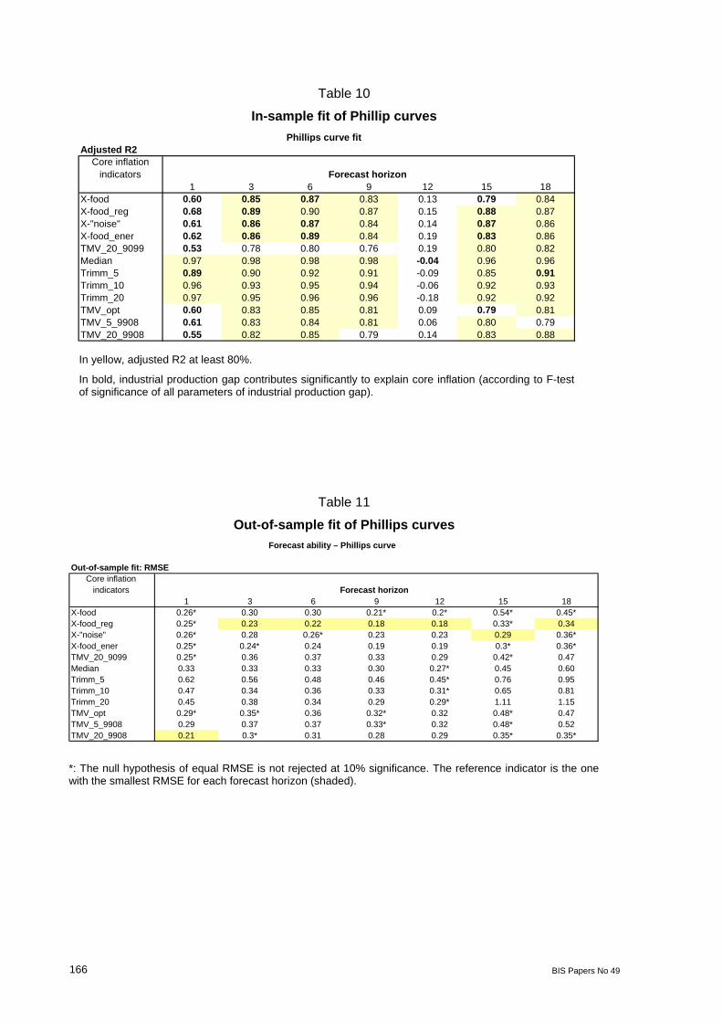
166 BIS Papers No 49
Table 10
In-sample fit of Phillip curves
In yellow, adjusted R2 at least 80%.
In bold, industrial production gap contributes significantly to explain core inflation (according to F-test of significance of all parameters of industrial production gap).
Table 11
Out-of-sample fit of Phillips curves
*: The null hypothesis of equal RMSE is not rejected at 10% significance. The reference indicator is the one with the smallest RMSE for each forecast horizon (shaded).
Phillips curve fitAdjusted R2
Core inflation indicators Forecast horizon
1 3 6 9 12 15 18 X-food 0.60 0.85 0.87 0.83 0.13 0.79 0.84 X-food_reg 0.68 0.89 0.90 0.87 0.15 0.88 0.87 X-"noise" 0.61 0.86 0.87 0.84 0.14 0.87 0.86 X-food_ener 0.62 0.86 0.89 0.84 0.19 0.83 0.86 TMV_20_9099 0.53 0.78 0.80 0.76 0.19 0.80 0.82 Median 0.97 0.98 0.98 0.98 -0.04 0.96 0.96 Trimm_5 0.89 0.90 0.92 0.91 -0.09 0.85 0.91 Trimm_10 0.96 0.93 0.95 0.94 -0.06 0.92 0.93 Trimm_20 0.97 0.95 0.96 0.96 -0.18 0.92 0.92 TMV_opt 0.60 0.83 0.85 0.81 0.09 0.79 0.81 TMV_5_9908 0.61 0.83 0.84 0.81 0.06 0.80 0.79 TMV_20_9908 0.55 0.82 0.85 0.79 0.14 0.83 0.88
Forecast ability – Phillips curve
Out-of-sample fit: RMSECore inflation
indicators Forecast horizon1 3 6 9 12 15 18
X-food 0.26* 0.30 0.30 0.21* 0.2* 0.54* 0.45*X-food_reg 0.25* 0.23 0.22 0.18 0.18 0.33* 0.34X-"noise" 0.26* 0.28 0.26* 0.23 0.23 0.29 0.36*X-food_ener 0.25* 0.24* 0.24 0.19 0.19 0.3* 0.36*TMV_20_9099 0.25* 0.36 0.37 0.33 0.29 0.42* 0.47Median 0.33 0.33 0.33 0.30 0.27* 0.45 0.60Trimm_5 0.62 0.56 0.48 0.46 0.45* 0.76 0.95Trimm_10 0.47 0.34 0.36 0.33 0.31* 0.65 0.81Trimm_20 0.45 0.38 0.34 0.29 0.29* 1.11 1.15TMV_opt 0.29* 0.35* 0.36 0.32* 0.32 0.48* 0.47TMV_5_9908 0.29 0.37 0.37 0.33* 0.32 0.48* 0.52TMV_20_9908 0.21 0.3* 0.31 0.28 0.29 0.35* 0.35*
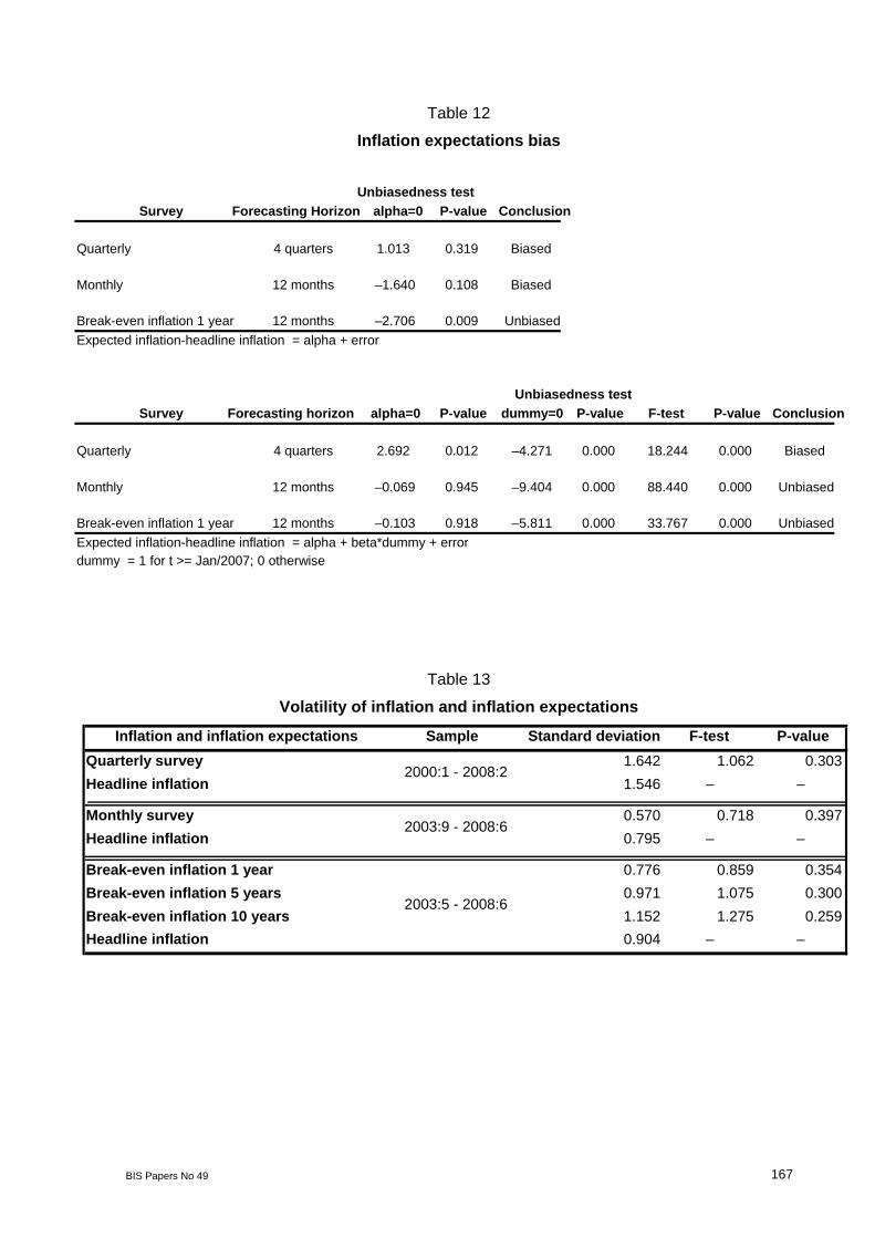
BIS Papers No 49 167
Table 12
Inflation expectations bias
Table 13
Volatility of inflation and inflation expectations
Unbiasedness test
Survey Forecasting Horizon alpha=0 P-value Conclusion
Quarterly 4 quarters 1.013 0.319 Biased
Monthly 12 months –1.640 0.108 Biased
Break-even inflation 1 year 12 months –2.706 0.009 Unbiased
Expected inflation-headline inflation = alpha + error
Survey Forecasting horizon alpha=0 P-value dummy=0 P-value F-test P-value Conclusion
Quarterly 4 quarters 2.692 0.012 –4.271 0.000 18.244 0.000 Biased
Monthly 12 months –0.069 0.945 –9.404 0.000 88.440 0.000 Unbiased
Break-even inflation 1 year 12 months –0.103 0.918 –5.811 0.000 33.767 0.000 Unbiased
Expected inflation-headline inflation = alpha + beta*dummy + errordummy = 1 for t >= Jan/2007; 0 otherwise
Unbiasedness test
Inflation and inflation expectations Sample Standard deviation F-test P-value
Quarterly survey 1.642 1.062 0.303 Headline inflation 1.546 – –
Monthly survey 0.570 0.718 0.397 Headline inflation 0.795 – –
Break-even inflation 1 year 0.776 0.859 0.354 Break-even inflation 5 years 0.971 1.075 0.300 Break-even inflation 10 years 1.152 1.275 0.259 Headline inflation 0.904 – –
2000:1 - 2008:2
2003:9 - 2008:6
2003:5 - 2008:6
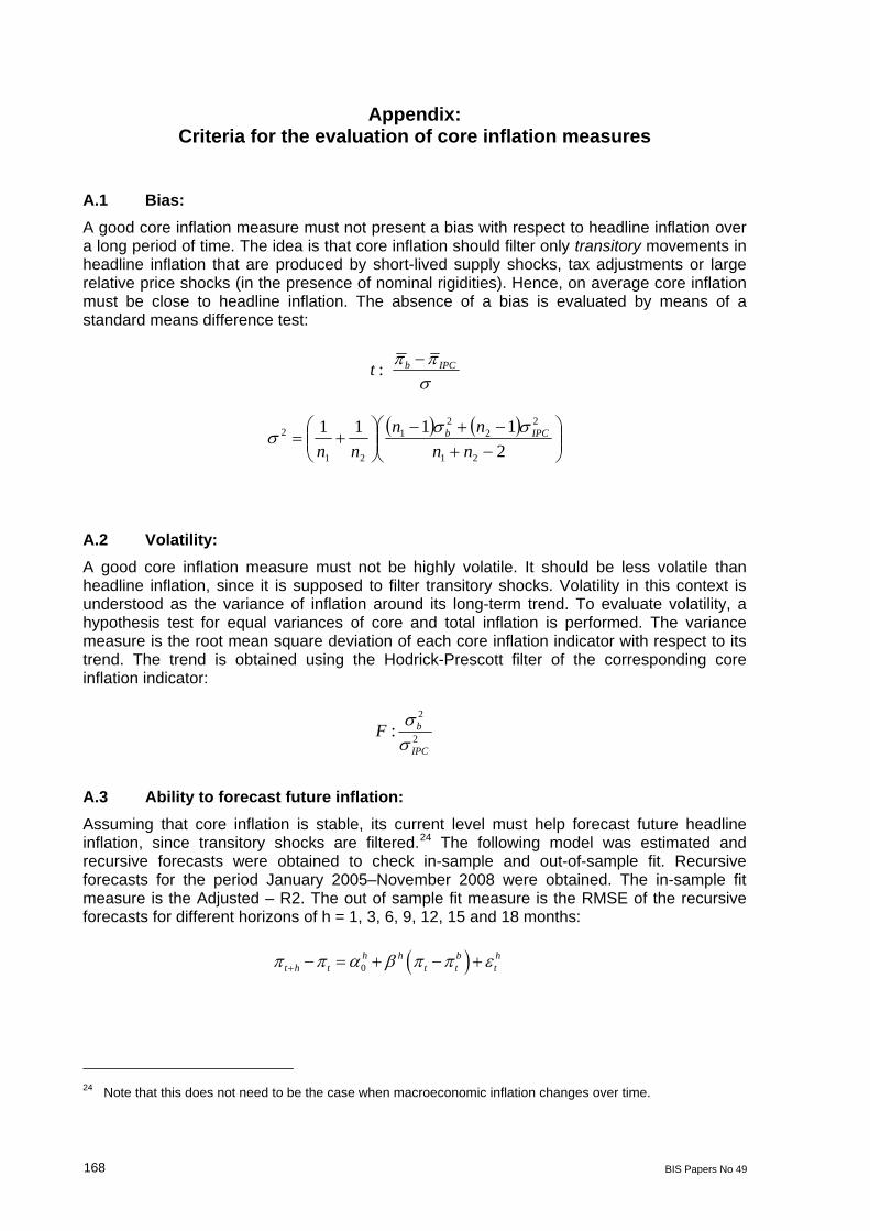
168 BIS Papers No 49
Appendix: Criteria for the evaluation of core inflation measures
A.1 Bias:
A good core inflation measure must not present a bias with respect to headline inflation over a long period of time. The idea is that core inflation should filter only transitory movements in headline inflation that are produced by short-lived supply shocks, tax adjustments or large relative price shocks (in the presence of nominal rigidities). Hence, on average core inflation must be close to headline inflation. The absence of a bias is evaluated by means of a standard means difference test:
IPCbt :
21111
21
22
21
21
2
nnnn
nnIPCb
A.2 Volatility:
A good core inflation measure must not be highly volatile. It should be less volatile than headline inflation, since it is supposed to filter transitory shocks. Volatility in this context is understood as the variance of inflation around its long-term trend. To evaluate volatility, a hypothesis test for equal variances of core and total inflation is performed. The variance measure is the root mean square deviation of each core inflation indicator with respect to its trend. The trend is obtained using the Hodrick-Prescott filter of the corresponding core inflation indicator:
A.3 Ability to forecast future inflation:
Assuming that core inflation is stable, its current level must help forecast future headline inflation, since transitory shocks are filtered.24 The following model was estimated and recursive forecasts were obtained to check in-sample and out-of-sample fit. Recursive forecasts for the period January 2005–November 2008 were obtained. The in-sample fit measure is the Adjusted – R2. The out of sample fit measure is the RMSE of the recursive forecasts for different horizons of h = 1, 3, 6, 9, 12, 15 and 18 months:
24 Note that this does not need to be the case when macroeconomic inflation changes over time.
2
2
:IPC
bF
0h h b h
t h t t t t
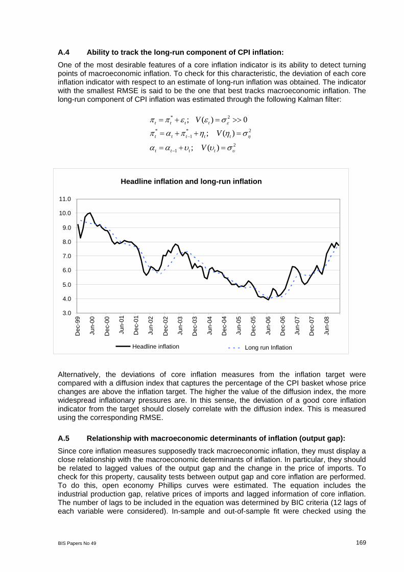
BIS Papers No 49 169
A.4 Ability to track the long-run component of CPI inflation:
One of the most desirable features of a core inflation indicator is its ability to detect turning points of macroeconomic inflation. To check for this characteristic, the deviation of each core inflation indicator with respect to an estimate of long-run inflation was obtained. The indicator with the smallest RMSE is said to be the one that best tracks macroeconomic inflation. The long-run component of CPI inflation was estimated through the following Kalman filter:
Alternatively, the deviations of core inflation measures from the inflation target were compared with a diffusion index that captures the percentage of the CPI basket whose price changes are above the inflation target. The higher the value of the diffusion index, the more widespread inflationary pressures are. In this sense, the deviation of a good core inflation indicator from the target should closely correlate with the diffusion index. This is measured using the corresponding RMSE.
A.5 Relationship with macroeconomic determinants of inflation (output gap):
Since core inflation measures supposedly track macroeconomic inflation, they must display a close relationship with the macroeconomic determinants of inflation. In particular, they should be related to lagged values of the output gap and the change in the price of imports. To check for this property, causality tests between output gap and core inflation are performed. To do this, open economy Phillips curves were estimated. The equation includes the industrial production gap, relative prices of imports and lagged information of core inflation. The number of lags to be included in the equation was determined by BIC criteria (12 lags of each variable were considered). In-sample and out-of-sample fit were checked using the
* 2
* * 21
21
; ( ) 0
; ( )
; ( )
t t t t
t t t t t
t t t t
VV
V
Headline inflation and long-run inflation
3.0
4.0
5.0
6.0
7.0
8.0
9.0
10.0
11.0
Dec
-99
Jun-
00
Dec
-00
Jun-
01
Dec
-01
Jun-
02
Dec
-02
Jun-
03
Dec
-03
Jun-
04
Dec
-04
Jun-
05
Dec
-05
Jun-
06
Dec
-06
Jun-
07
Dec
-07
Jun-
08
Headline inflation Long run Inflation

170 BIS Papers No 49
Adjusted – R2 and the RMSE of recursive out-of-sample forecasts for the period January 2006–November 2007. Additionally, we test the hypothesis of all the parameters associated to the IP-GAP be equal to zero:
, , 0 ,( ) ( ) ( )h h h h h m hb t h b t b t t t tL L y L
BIS Papers No 49 171
References
Arango, LE and Posada, CE (2006): “Los salarios de los funcionarios públicos en Colombia (1978–2005)”, Borradores de Economía no 417,. Banco de la República.
——— (2007): “El salario mínimo: aspectos generales sobre los casos de Colombia y otros países”, Borradores de Economía no 436, Banco de la República.
BBVA Economic Research Department (2008): Latinwatch, second semester.
Betancourt, YR, Jalil, M and M Misas (2009): “Before and after inflation targeting in Colombia”, Mimeo, Banco de la República.
Cecchetti, S (2007): “Core inflation”, Comment at the 2007 Dallas Fed Conference on measuring core inflation, May, www.dallasfed.org.
Gómez, J (2008): “Emerging Asia and international food inflation”, Borradores de Economía no 512, Banco de la República.
González, A and F Hamann (2006): “Lack of credibility, inflation persistence and disinflation in Colombia”, Mimeo, Banco de la República.
González, E, Jalil, M and JV Romero (2009): “Learning and biases in inflation expectations: an application for Colombia”, Mimeo, Banco de la República.
Henao, C (2008): “Inflacion objetivo en Colombia: aproximacion y evaluacion”, Monograph, Facultad de Economía, Universidad de los Andes.
López, E (2008): “Algunos hechos estilizados sobre el comportamiento de los precios regulados en Colombia”, Borradores de Economía no 527, Banco de la República.
Maureira J and G Leyva (2008): “Forecasting the Chilean inflation in difficult times”, XIII Meeting of the Researchers Network, CEMLA.
Rich, R and C Steindel (2007): “A comparison of measures of core inflation”, Federal Reserve Bank of New York, 8 May.
Rincón, H (2008): “¿Los consumidores colombianos de combustibles reciben subsidios o, en neto, pagan impuestos? Borradores de Economía no 540, Banco de la República.
Vargas, H (2007): “The transmission mechanism of monetary policy in Colombia: major changes and current features”, Borradores de Economía no 431, Banco de la República.