Modeling and Methodological Advances in Causal Inference
by
Shuxi Zeng
Department of Statistical ScienceDuke University
Date:Approved:
Fan Li, Advisor
Surya T. Tokdar
Jason Xu
Susan C. Alberts
Dissertation submitted in partial fulfillment of the requirements for the degree ofDoctor of Philosophy in the Department of Statistical Science
in the Graduate School of Duke University
2021

ABSTRACT
Modeling and Methodological Advances in Causal Inference
by
Shuxi Zeng
Department of Statistical ScienceDuke University
Date:Approved:
Fan Li, Advisor
Surya T. Tokdar
Jason Xu
Susan C. Alberts
An abstract of a dissertation submitted in partial fulfillment of the requirements forthe degree of Doctor of Philosophy in the Department of Statistical Science
in the Graduate School of Duke University
2021

Copyright © 2021 by Shuxi Zeng
All rights reserved

Abstract
This thesis develops novel theory, methods, and models in three major areas in causal
inference: (i) propensity score weighting methods for randomized experiments and
observational studies; (ii) causal mediation analysis with sparse and irregular longi-
tudinal data; and (iii) machine learning methods for causal inference. All theoretical
and methodological developments are accompanied by extensive simulation studies
and real world applications.
Our contribution to propensity score weighting method is presented in Chapter 2
and 3. In Chapter 2, we investigate the use of propensity score weighting in the ran-
domized trials for covariate adjustment. We introduce the class of balancing weights
and establish its theoretical properties. We demonstrate that it is asymptotically
equivalent to the analysis of covariance (ANCOVA) and derive the closed-form vari-
ance estimator. We further recommend the overlap weighting estimator based on
its semiparametric efficiency and good finite-sample performance. In Chapter 3, We
proposed a class of propensity score weighting estimators causal inference for survival
outcomes based on the pseudo-observations. This class of estimators are applicable to
several different target populations, survival causal estimands, as well as binary and
multiple treatments. We study the theoretical properties of the weighting estimator
and derive a new closed-form variance estimator.
Our contribution to causal mediation analysis is presented in Chapter 4. Causal
mediation analysis studies the causal relationships between treatment, outcome and
an intermediate variable (i.e. mediator) that lies in between. We extend the existing
causal mediation framework to the setting where both the mediator and outcome
are measured repeatedly on sparse and irregular time grids. We view the observed
mediator and outcome trajectories as realizations of underlying smooth stochastic
processes and define causal estimands of direct and indirect effects accordingly. We
provide assumptions to nonparametrically identify these estimands. We further de-
iv

vise a functional principal component analysis (FPCA) approach to estimate the
smooth processes and consequently causal effects. We adopt the Bayesian paradigm
to properly quantify the uncertainties in estimation.
Our contribution to machine learning methods for causal inference is presented in
Chapter 5 and 6. In Chapter 5, we develop a new algorithm that learns double-robust
representations in observational studies, leading to consistent causal estimation if the
model for either the propensity score or the outcome, but not necessarily both, is
correctly specified. Specifically, we use the entropy balancing method to learn the
weights that minimize the Jensen-Shannon divergence of the representation between
the treated and control groups, based on which we make robust and efficient coun-
terfactual predictions for both individual and average treatment effects. In Chapter
6, we study how to build a robust prediction model by exploiting the causal relation-
ships among predictors. We propose a causal transfer random forest method learning
the stable causal relationships efficiently from a large scale of observational data and
a small amount of randomized data. We provide theoretical justifications and vali-
date the algorithm empirically with synthetic experiments and real world prediction
tasks.
v

Contents
Abstract iv
List of Tables xi
List of Figures xiii
Acknowledgements xv
1 Introduction 2
1.1 Motivation . . . . . . . . . . . . . . . . . . . . . . . . . . . . . . . . . 2
1.2 Research questions and main contributions . . . . . . . . . . . . . . . 4
1.3 Outline . . . . . . . . . . . . . . . . . . . . . . . . . . . . . . . . . . . 8
2 Propensity score weighting in RCT 10
2.1 Introduction . . . . . . . . . . . . . . . . . . . . . . . . . . . . . . . . 10
2.2 Propensity score weighting for covariate adjustment . . . . . . . . . . 13
2.2.1 The balancing weights . . . . . . . . . . . . . . . . . . . . . . 13
2.2.2 The overlap weights . . . . . . . . . . . . . . . . . . . . . . . . 16
2.3 Efficiency considerations and variance estimation . . . . . . . . . . . 18
2.3.1 Continuous outcomes . . . . . . . . . . . . . . . . . . . . . . . 19
2.3.2 Binary outcomes . . . . . . . . . . . . . . . . . . . . . . . . . 21
2.3.3 Variance estimation . . . . . . . . . . . . . . . . . . . . . . . . 22
2.4 Simulation studies . . . . . . . . . . . . . . . . . . . . . . . . . . . . 24
2.4.1 Simulation design . . . . . . . . . . . . . . . . . . . . . . . . . 24
2.4.2 Results on efficiency of point estimators . . . . . . . . . . . . 27
2.4.3 Results on variance and interval estimators . . . . . . . . . . . 29
vi

2.4.4 Simulation studies with binary outcomes . . . . . . . . . . . . 31
2.5 Application to the Best Apnea Interventions for Research Trial . . . . 31
2.6 Discussion . . . . . . . . . . . . . . . . . . . . . . . . . . . . . . . . . 36
3 Propensity score weighting for survival outcome 40
3.1 Introduction . . . . . . . . . . . . . . . . . . . . . . . . . . . . . . . . 40
3.2 Propensity score weighting with survival outcomes . . . . . . . . . . . 43
3.2.1 Time-to-event outcomes, causal estimands and assumptions . 43
3.2.2 Balancing weights with pseudo-observations . . . . . . . . . . 44
3.3 Theoretical properties . . . . . . . . . . . . . . . . . . . . . . . . . . 47
3.4 Simulation studies . . . . . . . . . . . . . . . . . . . . . . . . . . . . 53
3.4.1 Simulation design . . . . . . . . . . . . . . . . . . . . . . . . . 53
3.4.2 Simulation results . . . . . . . . . . . . . . . . . . . . . . . . . 55
3.5 Application to National Cancer Database . . . . . . . . . . . . . . . . 59
4 Mediation analysis with sparse and irregular longitudinal data 64
4.1 Introduction . . . . . . . . . . . . . . . . . . . . . . . . . . . . . . . . 64
4.2 Motivating application: early adversity, social bond and stress . . . . 67
4.2.1 Biological background . . . . . . . . . . . . . . . . . . . . . . 67
4.2.2 Data . . . . . . . . . . . . . . . . . . . . . . . . . . . . . . . . 69
4.3 Causal mediation framework . . . . . . . . . . . . . . . . . . . . . . . 71
4.3.1 Setup and causal estimands . . . . . . . . . . . . . . . . . . . 71
4.3.2 Identification assumptions . . . . . . . . . . . . . . . . . . . . 74
4.4 Modeling mediator and outcome via functional principal componentanalysis . . . . . . . . . . . . . . . . . . . . . . . . . . . . . . . . . . 77
4.5 Empirical application . . . . . . . . . . . . . . . . . . . . . . . . . . . 81
vii

4.5.1 Results of FPCA . . . . . . . . . . . . . . . . . . . . . . . . . 81
4.5.2 Results of causal mediation analysis . . . . . . . . . . . . . . . 84
4.6 Simulations . . . . . . . . . . . . . . . . . . . . . . . . . . . . . . . . 86
4.6.1 Simulation design . . . . . . . . . . . . . . . . . . . . . . . . . 86
4.6.2 Simulation results . . . . . . . . . . . . . . . . . . . . . . . . . 89
5 Double robust representation learning 91
5.1 Introduction . . . . . . . . . . . . . . . . . . . . . . . . . . . . . . . . 91
5.2 Background . . . . . . . . . . . . . . . . . . . . . . . . . . . . . . . . 93
5.2.1 Setup and assumptions . . . . . . . . . . . . . . . . . . . . . . 93
5.2.2 Related work . . . . . . . . . . . . . . . . . . . . . . . . . . . 94
5.3 Methodology . . . . . . . . . . . . . . . . . . . . . . . . . . . . . . . 97
5.3.1 Proposal: unifying covariate balance and representation learning 97
5.3.2 Practical implementation . . . . . . . . . . . . . . . . . . . . . 99
5.3.3 Theoretical properties . . . . . . . . . . . . . . . . . . . . . . 102
5.4 Experiments . . . . . . . . . . . . . . . . . . . . . . . . . . . . . . . . 104
5.4.1 Experimental setups . . . . . . . . . . . . . . . . . . . . . . . 105
5.4.2 Learned balanced representations . . . . . . . . . . . . . . . . 106
5.4.3 Performance on semi-synthetic or real-world dataset . . . . . . 108
5.4.4 High-dimensional performance and double robustness . . . . . 109
6 Causal transfer random forest 111
6.1 Introduction . . . . . . . . . . . . . . . . . . . . . . . . . . . . . . . . 111
6.2 Related work . . . . . . . . . . . . . . . . . . . . . . . . . . . . . . . 114
6.2.1 Off-policy learning in online systems . . . . . . . . . . . . . . 114
6.2.2 Transfer learning and domain adaptation . . . . . . . . . . . . 114
viii

6.2.3 Causality and invariant learning . . . . . . . . . . . . . . . . . 115
6.3 Causal Transfer Random Forest . . . . . . . . . . . . . . . . . . . . . 116
6.3.1 Problem setup . . . . . . . . . . . . . . . . . . . . . . . . . . . 116
6.3.2 Proposed algorithm . . . . . . . . . . . . . . . . . . . . . . . . 118
6.3.3 Interpretations from causal learning . . . . . . . . . . . . . . . 121
6.4 Experiments on synthetic data . . . . . . . . . . . . . . . . . . . . . . 123
6.4.1 Setup and baselines . . . . . . . . . . . . . . . . . . . . . . . . 123
6.4.2 Synthetic data with explicit mechanism . . . . . . . . . . . . . 124
6.4.3 Synthetic auction: implicit mechanism . . . . . . . . . . . . . 128
6.5 Experiments on real-world data . . . . . . . . . . . . . . . . . . . . . 130
6.5.1 Randomized experiment (R-data) . . . . . . . . . . . . . . . 130
6.5.2 Robustness to real-world data shifts . . . . . . . . . . . . . . . 131
6.5.3 End-to-end marketplace optimization . . . . . . . . . . . . . . 132
7 Conclusions 136
8 Appendix 141
8.1 Appendix for Chapter 2 . . . . . . . . . . . . . . . . . . . . . . . . . 141
8.1.1 Proofs of the propositions in Section 2.3 . . . . . . . . . . . . 141
8.1.2 Derivation of the asymptotic variance and its consistent esti-mator in Section 2.3 . . . . . . . . . . . . . . . . . . . . . . . 150
8.1.3 Variance estimator for τAIPW . . . . . . . . . . . . . . . . . . . 153
8.1.4 Additional simulations with binary outcomes . . . . . . . . . . 154
8.1.5 Additional tables . . . . . . . . . . . . . . . . . . . . . . . . . 161
8.2 Appendix for Chapter 3 . . . . . . . . . . . . . . . . . . . . . . . . . 167
8.2.1 Proof of theoretical properties . . . . . . . . . . . . . . . . . . 167
ix

8.2.2 Details on simulation design . . . . . . . . . . . . . . . . . . . 182
8.2.3 Additional simulation results . . . . . . . . . . . . . . . . . . . 185
8.2.4 Additional information of the application . . . . . . . . . . . . 190
8.3 Appendix for Chapter 4 . . . . . . . . . . . . . . . . . . . . . . . . . 196
8.3.1 Proof of Theorem 3 . . . . . . . . . . . . . . . . . . . . . . . . 196
8.3.2 Gibbs sampler . . . . . . . . . . . . . . . . . . . . . . . . . . . 200
8.3.3 Individual imputed process . . . . . . . . . . . . . . . . . . . . 203
8.3.4 Simulation results for sample size N = 500, 1000 . . . . . . . . 204
8.4 Appendix for Chapter 5 . . . . . . . . . . . . . . . . . . . . . . . . . 207
8.4.1 Theorem proofs . . . . . . . . . . . . . . . . . . . . . . . . . . 207
8.4.2 Generalization to other estimands . . . . . . . . . . . . . . . . 214
8.4.3 Experiments details . . . . . . . . . . . . . . . . . . . . . . . . 216
8.5 Appendix for Chapter 6 . . . . . . . . . . . . . . . . . . . . . . . . . 218
8.5.1 Details on experiments . . . . . . . . . . . . . . . . . . . . . . 218
8.5.2 Proof for theorems . . . . . . . . . . . . . . . . . . . . . . . . 220
Bibliography 222
Biography 248
x

List of Tables
2.1 Performance comparison under different scenarios for continuous out-comes in simulated RCT. . . . . . . . . . . . . . . . . . . . . . . . . . 30
2.2 Baseline balance check for BestAIR study. . . . . . . . . . . . . . . . 33
2.3 Results for application in BestAIR study. . . . . . . . . . . . . . . . . 35
3.1 Simulation results for zero treatment effect under different scenarios. . 58
3.2 Results in NCDB application. . . . . . . . . . . . . . . . . . . . . . . 63
4.1 Summary of early adversity conditions in baboon study. . . . . . . . . 69
4.2 Mediation analysis results for baboon study. . . . . . . . . . . . . . . 85
4.3 Performance comparison for mediation analysis in simulations. . . . . 90
5.1 Results comparison on benchmark dataset for DRRL. . . . . . . . . . 108
6.1 Performance comparison in real-world click predictions. . . . . . . . . 132
6.2 Performance comparison in real-world tuning tasks. . . . . . . . . . . 134
8.1 Performance comparison with continuous outcomes in simulated RCT. 163
8.2 Performance comparison with binary outcomes in simulated RCT, sce-nario (a)-(d). . . . . . . . . . . . . . . . . . . . . . . . . . . . . . . . 164
8.3 Performance comparison with binary outcomes in simulated RCT, sce-nario (e)-(h). . . . . . . . . . . . . . . . . . . . . . . . . . . . . . . . 165
8.4 Non convergence frequency with binary outcomes in simulated RCT. 166
8.5 Simulation results with non-zero treatment effect under different sce-narios. . . . . . . . . . . . . . . . . . . . . . . . . . . . . . . . . . . . 189
8.6 Descriptive statistics of NCDB application. . . . . . . . . . . . . . . . 190
xi

8.7 Additional simulations results for mediation analysis. . . . . . . . . . 206
8.8 Hyperparameter choices . . . . . . . . . . . . . . . . . . . . . . . . . 216
8.9 Comparison for distribution shifts in tuning tasks. . . . . . . . . . . . 220
xii

List of Figures
2.1 Performance comparison with continuous outcomes for simulated RCT. 28
3.1 Simulation results under poor overlap. . . . . . . . . . . . . . . . . . 56
3.2 Weighted survival curves in NCDB application. . . . . . . . . . . . . 61
3.3 Estimated survival curves in NCDB application. . . . . . . . . . . . . 61
4.1 Individual trajectories of sparse mediator and outcomes in baboon study. 71
4.2 Graphical illustration of violation to Assumptions 1,2. . . . . . . . . . 76
4.3 Functional principal components of mediator and outcome process. . 82
4.4 Functional principal component analysis results in baboon study. . . . 83
4.5 Simulation results for mediation analysis against sparsity level. . . . . 89
5.1 Relationship between the entropy of weights and covariates balance. . 97
5.2 Architecture of the DRRL network . . . . . . . . . . . . . . . . . . . 100
5.3 Lower dimension representations of learned representations. . . . . . . 107
5.4 Sensitivity performance against relative importance of balance. . . . . 107
5.5 Policy risk curves comparison. . . . . . . . . . . . . . . . . . . . . . . 110
6.1 Challenges from unstable relationships in click prediction. . . . . . . . 112
6.2 CTRF: building random forest from R-data and L-data . . . . . . . . . 119
6.3 Graphical illustration of causal relationships in online advertisementsystem. . . . . . . . . . . . . . . . . . . . . . . . . . . . . . . . . . . . 120
6.4 Graphical illustrations for L-data and R-data. . . . . . . . . . . . . 122
xiii

6.5 Three scenarios in simulation with explicit mechanisms. . . . . . . . . 124
6.6 AUC comparison in simulation with explicit mechanisms. . . . . . . . 126
6.7 Bias comparison in simulation with explicit mechanisms. . . . . . . . 127
6.8 Performance comparison in simulation with implicit mechanisms. . . 128
6.9 Procedures for simulating auctions. . . . . . . . . . . . . . . . . . . . 129
8.1 Performance comparison with binary outcomes in simulated RCT, sce-nario (a)-(d). . . . . . . . . . . . . . . . . . . . . . . . . . . . . . . . 157
8.2 Performance comparison with binary outcomes in simulated RCT, sce-nario (e)-(h). . . . . . . . . . . . . . . . . . . . . . . . . . . . . . . . 158
8.3 The distribution of true GPS in simulations. . . . . . . . . . . . . . . 183
8.4 Simulation results under good overlap. . . . . . . . . . . . . . . . . . 186
8.5 Simulation results with trimmed IPW. . . . . . . . . . . . . . . . . . 187
8.6 Simulation results with regression based on pseudo-observations. . . . 191
8.7 Simulation results with augmented weighting estimators. . . . . . . . 192
8.8 Simulation results with IPW-MAO, OW-MAO. . . . . . . . . . . . . 193
8.9 Simulation results with non-zero treatment effect. . . . . . . . . . . . 194
8.10 Performance comparison in simulated RCT. . . . . . . . . . . . . . . 195
8.11 Distribution of estimated GPS in NCDB application. . . . . . . . . . 195
8.12 Individual process imputations for mediator and outcome. . . . . . . 204
8.13 Additional results for mediation effect estimations in simulations. . . 205
xiv

Acknowledgements
I am very fortunate to spend the past four years in the Department of Statistical
Science, Duke University. I would like to express my appreciation to the amazing
people who make my life towards Ph.D. a valuable memory.
First, I want to thank my advisor, Dr. Fan Li, for being a great mentor in causal
inference research. I benefit tremendously from her way of approaching research
problems. During our first meeting, she proposed three pillars for being a “success-
ful” Ph.D. in statistics, which include mathematics, programming and writing skills.
Although I am far from being excel in all the three forementioned aspects, I have
made great progress with her help during my Ph.D. study.
I also would like to thank Dr. Peng Ding at University of California, Berkeley,
for his generous recommendation and guidance to the research of causal inference.
I thank Dr. Bo Li at Tsinghua University for leading me into the statistics. which
shapes the career path for an undergraduate with the Economics major.
I also want to thank my collaborators during my Ph.D. study. I particularly enjoy
working with those researchers on the same project, including Dr. Fan (Frank) Li,
Dr. Susan Alberts, Dr. Elizabeth Archie, Dr. Stacy Rosenbaum, Dr. Fernando
Campos, Dr. Elizabeth Lange, Dr. Rui Wang, Dr. Liangyuan Hu, Dr. Lawrence
Carin, Dr. Chenyang Tao, Dr. Shounak Datta, Serge Assaad, Paidamoyo Chapfuwa
and Dr. Jason Poulos.
I would also like to thank my other thesis committee members, Dr. Surya Tokdar,
Dr. Jason Xu and Dr. Susan Alberts for all the suggestions and discussions on my
research. I also thank Dr. Emre Kiciman, Dr. Denis Charles and Dr. Murat Bayir
for the collaboration on my summer project at Microsoft and Dr. Swati Rallapalli
for hosting my internship at Facebook. I would also like to thank the staff in our
department, Lori Rauch, Nicole Scott, Karen Whitesell, for being so supportive to
the students.
xv

I wish to thank Xu Chen, Bai Li, Jialiang Mao, Jiurui Tang and many others for
being great friends. I also enjoy the time spending with my cohort, Fan Bu, Federico
Ferrari, Yi Guo, Henry Kirveslahti, Heather Mathews, Hanyu Song. I appreciate the
research discussions and game play with Sheng Jiang. I also owe a debt of gratitude
to my rootmates, Kangnan Li and Keru Wu.
Finally, I want to thank my parents for all their constant support from the other
side of the Earth, which is the strongest motivation along my endeavour.
1

1
Introduction
1.1 Motivation
Causal inference, or counterfactual prediction, is central to decision making in health-
care, policy and social sciences (Imbens and Rubin, 2015). The topic of causal in-
ference concerns the causal effect of one specific treatment Ti ∈ T , e.g. evaluating
the treatment effect of a medicine, on certain outcomes Yi of interests, based on the
sample i = 1, 2, · · · , N drawn from a population. Rubin (1974) defines the causal
effect in potential outcomes framework, which posits a set of potential outcomes
Yi(t), t ∈ T for each unit and only one of them is observed depending on the treat-
ment assigned. Therefore, the fundamental problem in causal inference is to impute
the missing potential outcomes (Holland, 1986). In observational study, the treat-
ment assignment is usually depending on certain pretreatment covariates Xi, which
are also correlated with the potential outcomes. The direct comparison across differ-
ent treatment groups can be biased as the distributions of some important covariates
might imbalance across two groups, which is also known as the confounding problem
(VanderWeele and Shpitser, 2013).
Several approaches like direct regression adjustment, matching (Abadie and Im-
bens, 2006) and weighting (Hirano et al., 2003) have been employed to address the
confounding or adjust for the covariate imbalance. The use of propensity score
weighting (Rosenbaum and Rubin, 1983), defined as the probability of being treated,
e(x) = Pr(Ti = 1|Xi = x), has been used to adjust for confounding bias in the ob-
servational study. However, the performance of weighting method deteriorates due
to the extreme weights in severe imbalance scenario. This problem is pronounced
2

especially when the sample size is small, even in randomized controlled trials with
imbalance only by chance (Senn, 1989; Ciolino et al., 2015; Thompson et al., 2015).
Moreover, the propensity score weighting estimator is hard to adapt when the data
is of a particular structure, such as the case dealing with survival outcomes with cen-
soring (Austin, 2014; Mao et al., 2018). Commonly used propensity score weighting
estimator is usually coupled with certain survival models and thus is vulnerable to
model misspecifications (Austin, 2010a,b). Developing a propensity score weighting
estimator without depending on the outcome modeling assumptions is of method-
ological interests.
Researchers might be not only interested in evaluating the effect of a certain treat-
ment but also understanding the causal mechanism, especially how much of the effect
can be attributed to a mediator Mi, which is also known as the mediation analysis
(Baron and Kenny, 1986; Imai et al., 2010b). For example, in a motivating appli-
cation, researchers study how much of the effect from early adversity on the health
outcome can be explained by the social bonds among wild baboons (Rosenbaum
et al., 2020). However, the mediators and outcomes might be measured on a sparse
and irregular grid for each unit in practice. The sparse and irregularly-spaced longi-
tudinal data are increasingly popular nowadays, such as in electronic health records
(EHR), which brings challenges for modeling and inference on mediation analysis.
Recent advances in machine learning research has equipped causal inference with
useful modeling or learning tools (Johansson et al., 2016; Shalit et al., 2017; Zhang
et al., 2020). While the powerful techniques like neural networks have been added
into the toolbox for outcome modeling, the importance of modeling the treatment
assignment mechanism has not been fully recognized in machine learning community.
Classic causal inference literature points out that combining both the propensity score
and the outcome model can increase the efficiency of the estimator and bring the dou-
bly robust property (Scharfstein et al., 1999; Lunceford and Davidian, 2004b; Kang
et al., 2007; Chernozhukov et al., 2018). Namely, the estimator remains consistent if
3

either the outcome or the propensity score model is correctly specified. One natural
question is how to attain the double robustness when we are faced with the high-
dimensional dataset and employ the machine learning algorithms, like representation
learning, for counterfactual predictions.
Causal inference also sheds light on other research areas such as the domain
adaptation and transfer learning (Quionero-Candela et al., 2009; Bickel et al., 2009;
Daume III and Marcu, 2006), even in the context without specific treatments. For
instance, one obstacle for a model to transfer from training distribution to a target
testing distribution is the spurious correlations. Namely, the algorithms exploiting
the correlations might learn the non-robust relationships that do not hold on the
testing data. One possible fix to use the direct causes of the labels, as the causal re-
lationships are expected to be robust across different scenarios (Rojas-Carulla et al.,
2018; Meinshausen, 2018; Kuang et al., 2018; Arjovsky et al., 2019). Some ads pub-
lisher (e.g. Bing ads) have run certain randomized experiments in the real traffic
to build robust models for click predictions (Bayir et al., 2019). However. the ran-
domized data are usually acquired at a larger cost and how to efficiently use it for
building robust prediction model is of particular interests to many practitioners.
1.2 Research questions and main contributions
Motivated by the specific challenges in causal inference, this thesis proposes the
several novel methods and modeling techniques. In this section, we briefly summarize
the research questions and highlight the contributions of the thesis.
1.Propensity score weighting in randomized controlled trials
Chance imbalance in baseline characteristics is common in randomized controlled
trials (RCT) (Senn, 1989; Ciolino et al., 2015). Regression adjustment such as the
analysis of covariance (ANCOVA) is often used to account for imbalance and increase
precision of the treatment effect estimate (Yang and Tsiatis, 2001; Kahan et al.,
2016; Leon et al., 2003; Tsiatis et al., 2008; Lin, 2013). An objective alternative is
4

through inverse probability weighting (IPW) of the propensity scores (Tsiatis et al.,
2008; Shen et al., 2014). Although IPW and ANCOVA are asymptotically equivalent
(Williamson et al., 2014), the former may demonstrate inferior performance in finite
samples. Whether we can retain the objectivity of weighting methods and meanwhile
improve the finite sample performance is of particular interests to the practitioners
analyzing the results for RCT.
In this thesis, we point out that IPW is a special case of the general class of
balancing weights (Li et al., 2018a), and advocate to use overlap weighting (OW)
for covariate adjustment. The OW method has a unique advantage of completely
removing chance imbalance when the propensity score is estimated by logistic re-
gression. We show that the OW estimator attains the same semiparametric variance
lower bound as the most efficient ANCOVA estimator and the IPW estimator for a
continuous outcome, and derive closed-form variance estimators for OW when esti-
mating additive and ratio estimands. Through extensive simulations, we demonstrate
OW consistently outperforms IPW in finite samples and improves the efficiency over
ANCOVA and augmented IPW when the degree of treatment effect heterogeneity is
moderate or when the outcome model is incorrectly specified.
2.Propensity score weighting with survival outcomes
Survival outcomes are common in comparative effectiveness studies. A standard
approach for causal inference with survival outcomes is to fit a Cox proportional
hazards model to an inversely probability weighted (IPW) sample (Austin, 2014;
Austin and Stuart, 2017). However, this method is subject to model misspecification
and the resulting hazard ratio estimate lacks causal interpretation (Hernan, 2010).
Moreover, IPW often corresponds to an inappropriate target population when there
is lack of covariate overlap between the treatment groups. A “once for all” approach
constructs “pseudo” observations of the censored outcomes and allows less-model
dependent methods such as propensity score weighting to proceed as if we have the
completely observed outcomes (Andersen et al., 2017).
5

3.Causal mediation analysis with sparse and irregular data
Causal mediation analysis seeks to investigate how the treatment effect of an ex-
posure on outcomes is mediated through intermediate variables (Robins and Green-
land, 1992; Pearl, 2001; Sobel, 2008; Tchetgen Tchetgen and Shpitser, 2012; Daniels
et al., 2012; VanderWeele, 2016). Although many applications involve longitudinal
data (van der Laan and Petersen, 2008; Roth and MacKinnon, 2012), the existing
methods are not directly applicable to settings where the mediator and outcome are
measured on sparse and irregular time grids.
This thesis extends the existing causal mediation framework from a functional
data analysis perspective, viewing the sparse and irregular longitudinal data as re-
alizations of underlying smooth stochastic processes. We define causal estimands
of direct and indirect effects accordingly and provide corresponding identification as-
sumptions. For estimation and inference, we employ a functional principal component
analysis approach for dimension reduction and use the first few functional principal
components instead of the whole trajectories in the structural equation models (Yao
et al., 2005; Jiang and Wang, 2010, 2011; Han et al., 2018). We adopt the Bayesian
paradigm to accurately quantify the uncertainties (Kowal and Bourgeois, 2020). The
operating characteristics of the proposed methods are examined via simulations. We
apply the proposed methods to a longitudinal data set from a wild baboon popula-
tion in Kenya to investigate the causal relationships between early adversity, strength
of social bonds between animals, and adult glucocorticoid hormone concentrations
(Rosenbaum et al., 2020).
4. Double robust representation learning
To de-bias causal estimators with high-dimensional data in observational studies,
recent advances suggest the importance of combining machine learning models for
both the propensity score and the outcome function (Belloni et al., 2014). Especially,
(Chernozhukov et al., 2018) proposed to combine machine learning models for the
propensity score and the outcome function to achieve√N consistency in estimating
6

the average treatment effect (ATE). A closely related concept is double-robustness
(Scharfstein et al., 1999; Lunceford and Davidian, 2004b; Kang et al., 2007), in which
an estimator is consistent if either the propensity score model or the outcome model,
but not necessarily both, is correctly specified.
This thesis proposes a novel scalable method to learn double-robust representa-
tions for counterfactual predictions, leading to consistent causal estimation if the
model for either the propensity score or the outcome, but not necessarily both, is
correctly specified. Specifically, we use the entropy balancing method (Hainmueller,
2012) to learn the weights that minimize the Jensen-Shannon divergence of the rep-
resentation between the treated and control groups, based on which we make robust
and efficient counterfactual predictions for both individual and average treatment ef-
fects. We provide theoretical justifications for the proposed method. The algorithm
shows competitive performance with the state-of-the-art on real world and synthetic
data.
5. Transfer learning based on causal relationships
It is often critical for prediction models to be robust to distributional shifts be-
tween training and testing data. From a causal perspective, the challenge is to
distinguish the stable causal relationships from the unstable spurious correlations
across shifts (Peters et al., 2016; Rojas-Carulla et al., 2018; Arjovsky et al., 2019).
An efficient algorithm to disentangle the stable causal relationships from the a large
amount of observational data and a small proportion of randomized data is of in-
terests to many practitioners especially for the online advertisement industry (Cook
et al., 2002; Kallus et al., 2018; Bayir et al., 2019).
We describe a causal transfer random forest (CTRF) that combines existing train-
ing data with a small amount of data from a randomized experiment to train a model
which is robust to the feature shifts and therefore transfers to a new targeting dis-
tribution. Theoretically, we justify the robustness of the approach against feature
shifts with the knowledge from causal learning. Empirically, we evaluate the CTRF
7

using both synthetic data experiments and real-world experiments in the Bing Ads
platform, including a click prediction task and in the context of an end-to-end coun-
terfactual optimization system. The proposed CTRF produces robust predictions
and outperforms most baseline methods compared in the presence of feature shifts.
1.3 Outline
In Chapter 2, we study the use of a general class of propensity score weights, called the
balancing weights in randomized trials for covariate adjustment. Within this class, we
advocate to use the overlap weighting (OW). We provide theoretical guarantee and
carry out extensive simulations studies on the proposed estimator. It turns out the
propensity score weighting estimator based on OW achieves semiparametric efficiency
under certain conditions as well as a good finite-sample performance.
In Chapter 3, we generalize the balancing weights in Li et al. (2018a) to time-to-
event outcomes based on the pseudo-observation approach with multiple treatments.
We study its theoretical property and derive closed-form variance estimators. The
variance estimators account for the uncertainty from propensity score estimation as
well as the pseudo observations. We examine both the point estimator and variance
estimator through extensive simulations and compare it with a range of commonly
used estimators.
In Chapter 4, we propose a causal mediation framework for sparse and irregular
longitudinal data. We view the data from a functional data analysis perspective and
define causal estimands of direct and indirect effects accordingly. We provide assump-
tions for nonparametric identification and modeling techniques based on functional
principal component analysis (FPCA). We project the mediator and outcome trajec-
tories to a low-dimensional representation and quantify the uncertainties accurately
through a Bayesian paradigm.
In Chapter 5, we propose a novel algorithm to learn the double-robust representa-
tions for counterfactual predictions in observational studies, allowing for simultaneous
8

learning of the representations and balancing weights. We study its theoretical prop-
erty and test its performance on several benchmark datasets. Though the proposed
method is motivated by estimating the treatment on average, it also demonstrates
comparable performance with state-of-the-art for individual treatment effects (ITE)
estimation.
In Chapter 6, we introduce a novel and efficient method for building robust pre-
diction models that combine large-scale observational data with a small amount of
randomized data. We also offer a theoretical justification of the proposed method
and its improved performance from the causal perspective. We evaluate the pro-
posed method with synthetic experiments and multiple experiments in a real-world,
large-scale online system at Bing Ads.
In Chapter 7, we conclude the thesis with highlights on the contributions and
directions for future extensions.
9
2
Propensity score weighting in RCT
2.1 Introduction
Randomized controlled trials are the gold standard for evaluating the efficacy and
safety of new treatments and interventions. Statistically, randomization ensures the
optimal internal validity and balances both measured and unmeasured confounders
in expectation. This makes the simple unadjusted difference-in-means estimator un-
biased for the intervention effect (Rosenberger and Lachin, 2002). Frequently, impor-
tant patient characteristics are collected at baseline; although over repeated experi-
ments, they will be balanced between treatment arms, chance imbalance often arises
in a single trial due to the random nature in allocating the treatment (Senn, 1989;
Ciolino et al., 2015), especially when the sample size is limited (Thompson et al.,
2015). If any of the baseline covariates are prognostic risk factors that are predictive
of the outcome, adjusting for the imbalance of these factors in the analysis can im-
prove the statistical power and provide a greater chance of identifying the treatment
signals when they actually exist (Ciolino et al., 2015; Pocock et al., 2002; Hernandez
et al., 2004).
There are two general streams of methods for covariate adjustment in randomized
trials: (outcome) regression adjustment (Yang and Tsiatis, 2001; Kahan et al., 2016;
Leon et al., 2003; Tsiatis et al., 2008; Zhang et al., 2008) and the inverse probability
of treatment weighting (IPW or IPTW) based on propensity scores (Williamson
et al., 2014; Shen et al., 2014; Colantuoni and Rosenblum, 2015). For regression
adjustment with continuous outcomes, the analysis of covariance (ANCOVA) model is
often used, where the outcome is regressed on the treatment, covariates and possibly
10

their interactions (Tsiatis et al., 2008). The treatment effect is estimated by the
coefficient of the treatment variable. With binary outcomes, a generalized linear
model can be postulated to estimate the adjusted risk ratio or odds ratio, with the
caveat that the regression coefficient of treatment may not represent the marginal
effect due to non-collapsability (Williamson et al., 2014). Tsiatis and co-authors
developed a suite of semiparametric ANCOVA estimators that improves efficiency
over the unadjusted analysis in randomized trials (Yang and Tsiatis, 2001; Leon et al.,
2003; Tsiatis et al., 2008). Lin (Lin, 2013) clarified that it is critical to incorporate
covariate-by-treatment interaction terms in regression adjustment for efficiency gain.
When the randomization probability is 1/2, ANCOVA returns consistent point and
interval estimates even if the outcome model is misspecified (Yang and Tsiatis, 2001;
Lin, 2013; Wang et al., 2019). However, misspecification of the outcome model can
decrease precision in unbalanced experiments with treatment effect heterogeneity
(Freedman, 2008). Another limitation of regression adjustment is the potential for
inviting a ‘fishing expedition’: one may search for an outcome model that gives the
most dramatic treatment effect estimate which jeopardizes the objectivity of causal
inference with randomized trials (Tsiatis et al., 2008; Shen et al., 2014).
Originally developed in the context of survey sampling and observational studies
(Lunceford and Davidian, 2004a), IPW has been advocated as an objective alterna-
tive to ANCOVA in randomized trials (Williamson et al., 2014). To implement IPW,
one first fits a logistic working model to estimate the propensity scores – the condi-
tional probability of receiving the treatment given the baseline covariates (Rosenbaum
and Rubin, 1983), and then estimates the treatment effect by the difference of the
weighted outcome – weighted by the inverse of the estimated propensity – between the
treatment arms. In randomized trials, the treatment group is randomly assigned and
the true propensity score is known. Therefore, the working propensity score model is
always correctly specified, and the IPW estimator is consistent to the marginal treat-
ment effect. For a continuous outcome, the IPW estimator with a logistic propensity
11

model has the same large-sample variance as the efficient ANCOVA estimator (Shen
et al., 2014; Williamson et al., 2014), but it offers the following advantages.
First, IPW separates the design and analysis in the sense that the propensity
score model only involves baseline covariates and the treatment indicator; it does
not require the access to the outcome and hence avoids the ‘fishing expedition.’ As
such, IPW offers better transparency and objectivity in pre-specifying the analytical
adjustment before outcomes are observed. Second, IPW preserves the marginal treat-
ment effect estimand with non-continuous outcomes, while the interpretation of the
outcome regression coefficient may change according to different covariate specifica-
tions (Hauck et al., 1998; Robinson and Jewell, 1991). Third, IPW can easily obtain
treatment effect estimates for rare binary or categorical outcomes whereas outcome
models often fail to converge in such situations (Williamson et al., 2014). This is
particularly the case when the target parameter is a risk ratio, where log-binomial
models are known to have unsatisfying convergence properties (Zou, 2004). On the
other hand, a major limitation of IPW is that it may be inefficient compared to AN-
COVA with limited sample sizes and unbalanced treatment allocations (Raad et al.,
2020) .
In this chapter, we point out that IPW is a special case of the general class of
propensity score weights, called the balancing weights (Li et al., 2018a), many mem-
bers of which could be used for covariate adjustment in randomized trials. Within
this class, we advocate to use the overlap weighting (OW) (Li et al., 2018a, 2019;
Schneider et al., 2001; Crump et al., 2006; Li and Li, 2019b). In the context of
randomized trials, a particularly attractive feature of OW is that, if the propensity
score is estimated from a logistic working model, then OW leads to exact mean bal-
ance of any baseline covariate in that model, and consequently remove the chance
imbalance of that covariate. As a propensity score method, OW retains the aforemen-
tioned advantages of IPW while offers better finite-sample properties (Section 2.2).
In Section 2.3, we demonstrate that the OW estimator, similar as IPW, achieves the
12

same semiparametric variance lower bound and hence is asymptotically equivalent to
the efficient ANCOVA estimator for continuous outcomes. For binary outcomes, we
further provide closed-form variance estimators of the OW estimator for estimating
marginal risk difference, risk ratio and odds ratio, which incorporates the uncertainty
in estimating the propensity scores and achieves close to nominal coverage in finite
samples. Through extensive simulations in Section 2.4, we demonstrate the effi-
ciency advantage of OW under small to moderate sample sizes, and also validate the
proposed variance estimator for OW. Finally, in Section 2.5 we apply the proposed
method to the Best Apnea Interventions for Research (BestAIR) randomized trial
and evaluate the treatment effect of continuous positive airway pressure (CPAP) on
several clinical outcomes.
2.2 Propensity score weighting for covariate adjustment
2.2.1 The balancing weights
We consider a randomized trial with two arms and N patients, where N1 and N0
patients are randomized into the treatment and control arm, respectively. Let Zi = z
be the binary treatment indicator, with z = 1 indicates treatment and z = 0 control.
Under the potential outcome framework (Neyman, 1990), each unit has a pair of
potential outcomes Yi(1), Yi(0), mapped to the treatment and control condition,
respectively, of which only the one corresponding to the actual treatment assigned
is observed. We denote the observed outcome as Yi = ZiYi(1) + (1 − Zi)Yi(0). In
randomized trials, a collection of p baseline variables could be recorded for each
patient, denoted by Xi = (Xi1, . . . , Xip)T . Denote µz = EYi(z) and µz(x) =
EYi(z)|Xi = x as the marginal and conditional expectation of the outcome in arm
z (z = 0, 1), respectively. A common estimand on the additive scale is the average
treatment effect (ATE):
τ = EYi(1)− Yi(0) = µ1 − µ0. (2.1)
13

We assume that the treatment Z is randomly assigned to patients, where Pr(Zi =
1|Xi, Yi(1), Yi(0)) = Pr(Zi = 1) = r, and 0 < r < 1 is the randomization probability
(see Section 8.1.1 for additional discussions on randomization). The most typical
study design uses balanced assignment with r = 1/2. Other values of r may be
possible, for example, when there is a perceived benefit of the treatment, and a larger
proportion of patients are randomized to the intervention. Under randomization of
treatment and the consistency assumption, we have τ = E(Yi|Zi = 1)−E(Yi|Zi = 0),
and thus the unadjusted difference-in-means estimator is:
τUNADJ =
∑Ni=1 ZiYi∑Ni=1 Zi
−∑N
i=1(1− Zi)Yi∑Ni=1(1− Zi)
. (2.2)
Below we generalize the ATE to a class of weighted average treatment effect
(WATE) estimands to construct alternative weighting methods. Assume the study
sample is drawn from a probability density f(x), and let g(x) denote the covariate
distribution density of a target population, possibly different from the one represented
by the observed sample. The ratio h(x) = g(x)/f(x) is called a tilting function (Li
and Li, 2019b), which re-weights the distribution of the baseline characteristics of
the study sample to represent the target population. We can represent the ATE on
the target population g by a WATE estimand:
τh = Eg[Yi(1)− Yi(0)] =Eh(x)(µ1(x)− µ0(x))
Eh(x). (2.3)
In practice, we usually pre-specify h(x) instead of g(x). Most commonly h(x) is
specified as a function of the propensity score or simply a constant. The propensity
score (Rosenbaum and Rubin, 1983) is the conditional probability of treatment given
the covariates, e(x) = Pr(Zi = 1|Xi = x). Under the randomization assumption,
e(x) = Pr(Zi = 1) = r for any baseline covariate value x, and therefore as long
as h(x) is a function of the propensity score e(x), different h corresponds to the
same target population g, and the WATE reduces to ATE, i.e. τh = τ . This is
distinct from observational studies, where the propensity scores are usually unknown
and vary between units, and consequently different h(x) corresponds to different
14

target populations and estimands (Thomas et al., 2020b). This special feature under
randomized trials provides the basis for considering alternative weighting strategies
to achieve better finite-sample performances.
In the context of confounding adjustment in observational studies, Li et al. pro-
posed a class of propensity score weights, named the balancing weights, to estimate
WATE(Li et al., 2018a). Specifically, given any h(x), the balancing weights for pa-
tients in the treatment and control arm are defined as:
w1(x) = h(x)/e(x), w0(x) = h(x)/1− e(x), (2.4)
which balances the distributions of the covariates between treatment and control
arms in the target population, so that f1(x)w1(x) = f0(x)w0(x) = f(x)h(x), where
fz(x) is the conditional distribution of covariates in treatment arm z (Wallace and
Moodie, 2015; Li et al., 2018a). Then, one can use the following Hajek-type estimator
to estimate τh:
τh = µh1 − µh0 =
∑Ni=1w1(xi)ZiYi∑Ni=1w1(xi)Zi
−∑N
i=1w0(xi)(1− Zi)Yi∑Ni=1w0(xi)(1− Zi)
. (2.5)
The function h(x) can take any form, each corresponding to a specific weighting
scheme. For example, when h(x) = 1, the balancing weights become the inverse
probability weights, (w1, w0) = (1/e(x), 1/1 − e(x)); when h(x) = e(x)(1 − e(x)),
we have the overlap weights (Li et al., 2018a), (w1, w0) = (1 − e(x), e(x)), which
was also independently developed by Wallace and Moodie (Wallace and Moodie,
2015) in the context of dynamic treatment regimes. Other examples of the balancing
weights include the average treatment effect among treated (ATT) weights (Hirano
and Imbens, 2001) and the matching weights (Li and Greene, 2013).
IPW is the most well-known case of the balancing weights. Specific to covariate
adjustment in randomized trials, Williamson et al. (Williamson et al., 2014) and
Shen et al. (Shen et al., 2014) suggested the following IPW estimator of τ :
τ IPW =
∑Ni=1 ZiYi/ei∑Ni=1 Zi/ei
−∑N
i=1(1− Zi)Yi/(1− ei)∑Ni=1(1− Zi)/(1− ei)
. (2.6)
15

We will point out in Section 2.3 that their findings on IPW are generally applicable to
the balancing weights as long as h(x) is a smooth function of the true propensity score.
The choice of h(x), however, will affect the finite-sample operating characteristics of
the weighting estimator. In particular, below we will closely examine the overlap
weights.
2.2.2 The overlap weights
In observational studies, the overlap weights correspond to a target population with
the most overlap in the baseline characteristics, and have been shown theoretically
to give the smallest asymptotic variance of τh among all balancing weights (Li et al.,
2018a) as well as empirically reduce the variance of τh in finite samples (Li et al.,
2019). Illustrative examples of the overlap population distribution can be found in
Figure 1 of Li et al. (Li et al., 2018a) with a single covariate as well as in the bubble
plot of Thomas et al. (Thomas et al., 2020a) with two covariates. In randomized
trials, as discussed before, because the true propensity score is constant, the overlap
weights and IPW target the same population estimand τ , but their finite-sample
operating characteristics can be markedly different, as elucidated below.
The OW estimator for the ATE in randomized trials is
τOW = µ1 − µ0 =
∑Ni=1(1− ei)ZiYi∑Ni=1(1− ei)Zi
−∑N
i=1 ei(1− Zi)Yi∑Ni=1 ei(1− Zi)
, (2.7)
where ei = e(Xi; θ) is the estimated propensity score from a working logistic regres-
sion model:
ei = e(Xi; θ) =exp(θ0 +XT
i θ1)
1 + exp(θ0 +XTi θ1)
, (2.8)
with parameters θ = (θ0, θT1 )T and θ is the maximum likelihood estimate of θ. Regard-
ing the selection of covariates in the propensity score model, the previous literature
suggests to include stratification variables as well as a small number of key prognostic
factors pre-specified in the design stage (Raab et al., 2000; Williamson et al., 2014).
These guidelines are also applicable to the OW estimator.
16

The logistic propensity score model fit underpins a unique exact balance property
of OW. Specifically, the overlap weights estimated from model (2.8) lead to exact
mean balance of any predictor included in the model (Theorem 3 in Li et al. (Li
et al., 2018a)):∑Ni=1(1− ei)ZiXji∑Ni=1(1− ei)Zi
−∑N
i=1 ei(1− Zi)Xji∑Ni=1 ei(1− Zi)
= 0, for j = 1, ..., p. (2.9)
This property has important practical implications in randomized trials, namely,
for any baseline covariate included in the propensity score model, the associated
chance imbalance in a single randomized trial vanishes once the overlap weights are
applied. If one reports the weighted mean differences in baseline covariates between
arms (frequently included in the standard “Table 1” in primary trial reports), those
differences are identically zero. Thus the application of OW enhances the face validity
of the randomized study.
More importantly, the exact mean balance property translates into better effi-
ciency in estimating τ . To illustrate the intuition, consider the following simple
example. Suppose the true outcome surface is Yi = α + Ziτ + XTi β0 + εi with
E(εi|Zi, Xi) = 0. Denote the weighted chance imbalance in the baseline covariates
by
∆X(w0, w1) =
∑Ni=1w1(Xi)ZiXi∑Ni=1w1(Xi)Zi
−∑N
i=1w0(Xi)(1− Zi)Xi∑Ni=1w0(Xi)(1− Zi)
,
and the weighted difference in random noise by
∆ε(w0, w1) =
∑Ni=1w1(Xi)Ziεi∑Ni=1 w1(Xi)Zi
−∑N
i=1 w0(Xi)(1− Zi)εi∑Ni=1w0(Xi)(1− Zi)
.
For the unadjusted estimator, substituting the true outcome surface in equation
(2.2) gives τUNADJ − τ = ∆X(1, 1)Tβ0 + ∆ε(1, 1).This expression implies that the
estimation error of τUNADJ is a sum of the chance imbalance and random noise, and
becomes large when imbalanced covariates are highly prognostic (i.e. large magnitude
of β0). Similarly, if we substitute the true outcome surface in (2.6), we can show
that the estimation error of IPW is τ IPW − τ = ∆X(1/(1 − e), 1/e)Tβ0 + ∆ε(1/(1 −
17

e), 1/e). Intuitively, IPW controls for chance imbalance because we usually have
‖∆X(1/(1− e), 1/e)‖ < ‖∆X(1, 1)‖, which reduces the variation of the estimation
error over repeated experiments. However, because ∆X(1/(1− e), 1/e) is not zero,
the estimation error remains sensitive to the magnitude of β0. In contrast, because
of the exact mean balance property of OW, we have ∆X(e, 1− e) = 0; consequently,
substituting the true outcome surface in (2.7), we can see that the estimation error
of OW equals τOW − τ = ∆ε(e, 1 − e), which is only noise and free of β0. This
simple example illustrates that, for each realized randomization, OW should have
the smallest estimation error, which translates into larger efficiency in estimating τ
over repeated experiments.
For non-continuous outcomes, we also consider ratio estimands. For example,
while the ATE is also known as the causal risk difference with binary outcomes,
τ = τRD. Two other standard estimands are the causal risk ratio (RR) and the causal
odds ratio (OR) on the log scale, defined by
τRR = log
(µ1
µ0
), τOR = log
µ1/(1− µ1)
µ0/(1− µ0)
. (2.10)
The OW estimator for risk ratio and odds ratio are τRR = logµ1/µ0, and τOR =
logµ1/(1− µ1)/µ0/(1− µ0), respectively, with µ1, µ0 defined in (2.7).
2.3 Efficiency considerations and variance estimation
In this section we demonstrate that in randomized trials the OW estimator leads to
increased large-sample efficiency in estimating the treatment effect compared to the
unadjusted estimator. We further propose a consistent variance estimator for the
OW estimator of both the additive and ratio estimands.
18

2.3.1 Continuous outcomes
Tsiatis et al. (Tsiatis et al., 2008) show that the family of regular and asymptotically
linear estimators for the additive estimand τ is
I :1
N
N∑i=1
ZiYir− (1− Zi)Yi
1− r− Zi − rr(1− r)
rg0(Xi) + (1− r)g1(Xi)
+ op(N−1/2),
(2.11)
where r is the randomization probability, and g0(Xi), g1(Xi) are scalar functions of the
baseline covariates Xi. Several commonly used estimators for the treatment effect are
members of the family I, with different specifications of g0(Xi), g1(Xi). For example,
setting g0(Xi) = g1(Xi) = 0, we obtain the unadjusted estimator τUNADJ. Setting
g0(Xi) = g1(Xi) = E(Yi|Xi), we obtain the “ANCOVA I” estimator in Yang and
Tsiatis (Yang and Tsiatis, 2001), which is the least-squares solution of the coefficient
of Zi in a linear regression of Yi on Zi and Xi. Further, setting g0(Xi) = E(Yi|Zi =
0, Xi) and g1(Xi) = E(Yi|Zi = 1, Xi), we obtain the “ANCOVA II” estimator (Yang
and Tsiatis, 2001; Tsiatis et al., 2008; Lin, 2013), which is the least-squares solution
of the coefficient of Zi in a linear regression of Yi on Zi, Xi and their interaction terms.
This estimator achieves the semiparametric variance lower bound within the family
I, when the conditional mean functions g0(Xi) and g1(Xi) are correctly specified in
the ANCOVA model (Robins et al., 1994; Leon et al., 2003). Another member of I
is the target maximum likelihood estimator (Moore and van der Laan, 2009; Moore
et al., 2011; Colantuoni and Rosenblum, 2015), which is asymptotic efficient under
correct outcome model specification. The IPW estimator τ IPW is also a member of I.
Specifically, Shen et al. (Shen et al., 2014) showed that if the logistic model (2.8) is
used to estimate the propensity score ei, then the IPW estimator is asymptotically
equivalent to the “ANCOVA II” estimator and becomes semiparametric efficient if
the true g0(Xi) and g1(Xi) are linear functions of Xi.
In the following Proposition we show that the OW estimator is also a member
of I and is asymptotically efficient under the linearity assumption. The proof of
19

Proposition 1 is provided in Section 8.1.1.
Proposition 1. (Asymptotic efficiency of overlap weighting)
(a) If the propensity score is estimated by a parametric model e(X; θ) with parameters
θ that satisfies a set of mild regularity conditions (specified in Section 8.1.1), then
τOW belongs to the class of estimators I.
(b) Suppose X1 and X2 are two nested sets of baseline covariates with X2 = (X1, X∗1),
and e(X1; θ1), e(X2; θ2) are nested smooth parametric models. Write τOW1 and τOW
2 as
two OW estimators with the weights defined through e(X1; θ1) and e(X2; θ2), respec-
tively. Then the asymptotic variance of τOW2 is no larger than that of τOW
1 .
(c) If the propensity score is estimated from the logistic regression (2.8), then τOW is
asymptotically equivalent to the “ANCOVA II” estimator, and becomes semiparamet-
ric efficient as long as the true E(Yi|Xi, Zi = 1) and E(Yi|Xi, Zi = 0) are linear in
Xi.
Proposition 1 summarizes the large-sample properties of the OW estimator in
randomized trials, extending those demonstrated for IPW in Shen et al (Shen et al.,
2014). In particular, adjusting for the baseline covariates using OW does not ad-
versely affect efficiency in large samples than without adjustment. Further, the
asymptotic equivalence between τOW and the “ANCOVA II” estimator indicates that
OW becomes fully semiparametric efficient when the conditional outcome surface is
a linear function of the covariates adjusted in the logistic propensity score model. In
the special case where the randomization probability r = 1/2, we show in Section
8.1.3 that the limit of the large-sample variance of τOW is
limN→∞
NVar(τOW) = (1−R2Y∼X) lim
N→∞NVar(τUNADJ) = 4(1−R2
Y∼X)Var(Yi), (2.12)
where Yi = Zi(Yi − µ1) + (1− Zi)(Yi − µ0) is the mean-centered outcome and R2Y∼X
measures the proportion of explained variance after regressing Yi on Xi. Similar defi-
nition of R-squared was also used elsewhere when demonstrating efficiency gain with
covariate adjustment (Moore and van der Laan, 2009; Moore et al., 2011; Wang et al.,
20

2019). The amount of variance reduction is also a direct result from the asymptotic
equivalence between the OW, IPW, and “ANCOVA II” estimators. Equation (2.12)
shows that incorporating additional covariates into the propensity score model will
not reduce the asymptotic efficiency because R2Y∼X is non-decreasing when more co-
variates are considered. Although adding covariates does not hurt the asymptotic
efficiency, in practice we recommend incorporating the covariates that exhibit base-
line imbalance and that have large predictive power for the outcome (Williamson
et al., 2014).
Perhaps more interestingly, the results in Proposition 1 apply more broadly to
the family of balancing weights estimators, formalized in the following Proposition.
The proof of Proposition 2 is presented in Section 8.1.1.
Proposition 2. (Extension to balancing weights)
Proposition 1 holds for the general family of estimators (2.5) using balancing weights
defined in (2.4), as long as the tilting function h(X) is a “smooth” function of the
propensity score, where “smooth” is defined by satisfying a set of mild regularity
conditions (specified in details in Section 8.1.1).
2.3.2 Binary outcomes
For binary outcomes, the target estimand could be the causal risk difference, risk
ratio and odds ratio, denoted as τRD, τRR and τOR, respectively. The discussions in
Section 2.3.1 directly apply to the estimation of the additive estimand, τRD. When
estimating the ratio estimands, one should proceed with caution in interpreting re-
gression parameters for the ANCOVA-type generalized linear models due to the po-
tential non-collapsibility issue. Additionally, it is well-known that the log-binomial
model frequently fails to converge with a number of covariates, and therefore one
may have to resort to less efficient regression methods such as the modified Poisson
regression (Zou, 2004). Williamson et al. (Williamson et al., 2014) showed that IPW
can be used to adjust for baseline covariates without changing the interpretation of
21

the marginal treatment effect estimands, τRR and τOR. Because of the asymptotic
equivalence between the IPW and OW estimators (Proposition 1), OW shares the
advantages of IPW in improving the asymptotic efficiency over the unadjusted esti-
mators for risk ratio and odds ratio without compromising the interpretation of the
marginal estimands. In addition, due to its ability to remove all chance imbalance
associated with Xi, OW is likely to give higher efficiency than IPW in finite samples,
which we will demonstrate in Section 2.4.
2.3.3 Variance estimation
To estimate the variance of the propensity score estimators, it is important to incor-
porate the uncertainty in estimating the propensity scores (Lunceford and Davidian,
2004a). Failing to do so leads to conservative variance estimates of the weighting esti-
mator and therefore reduces power of the Wald test for treatment effect (Williamson
et al., 2014). Below we use the M-estimation theory (Tsiatis, 2007) to derive a con-
sistent variance estimator for OW. Specifically, we cast µ1, µ0 in equation (2.7), and
θ in the logistic model (2.8) as the solutions λ = (µ1, µ0, θT )T to the following joint
estimation equations∑N
i=1 Ui =∑N
i=1 U(Yi, Xi, Zi; λ) = 0, where
n∑i=1
U(Yi, Xi, Zi, λ) =N∑i=1
Zi(Yi − µ1)(1− ei)(1− Zi)(Yi − µ0)ei
Xi(Zi − ei)
= 0, (2.13)
where Xi = (1, XTi )T is the augmented covariates with an intercept. Here, the first
two rows represent the estimating functions for µ1 and µ0 and the last rows are the
score functions of the logistic model with an intercept and main effects of Xi. If
Xi is of p dimensions, equation (2.13) involves p + 3 scalar estimating equations for
p + 3 parameters. Let A = −E(∂Ui/∂λ)T ,B = E(UiUTi ), the asymptotic covariance
matrix for λ can be written as N−1A−1BA−T . Extracting the covariance matrix for
the first two components in λ, we can show that, as N goes to infinity,
√N
[µ1 − µ1
µ0 − µ0
]→ N
0,
[Σ11,Σ12
Σ21,Σ22
], (2.14)
22

where the covariance matrix is defined as the corresponding elements in A−1BA−T ,
Σ11 = [A−1BA−T ]1,1,Σ22 = [A−1BA−T ]2,2,Σ12 = ΣT21 = [A−1BA−T ]1,2. (2.15)
where [A−1BA−T ]j,k denotes the (j, k)th element of the matrix A−1BA−T . Using the
delta method, we can obtain the asymptotic variance of τOWRD , τOW
RR , τOWOR as a function
of Σ11,Σ22,Σ12. Consistent plug-in estimators can then be obtained by estimating
the expectations in the “sandwich” matrix A−1BA−T by their corresponding sample
averages. We summarize the variance estimators for τOWRD , τ
OWRR , τ
OWOR in the following
general equations,
Var(τOW) =1
N
V UNADJ − vT1
1
N
N∑i=1
ei(1− ei)XTi Xi
−1
(2v1 − v2)
, (2.16)
where
V UNADJ =
1
N
N∑i=1
ei(1− ei)
−1
(E2
1
N1
N∑i=1
Ziei(1− ei)2(Yi − µ1)2 +E2
0
N0
N∑i=1
(1− Zi)e2i (1− ei)(Yi − µ0)2
),
v1 =
1
N
N∑i=1
ei(1− ei)
−1
(E1
N1
N∑i=1
Zie2i (1− ei)(Yi − µ1)2Xi +
E0
N0
N∑i=1
(1− Zi)ei(1− ei)2(Yi − µ0)2Xi
),
v2 =
1
N
N∑i=1
ei(1− ei)
−1
(E1
N1
N∑i=1
Ziei(1− ei)2(Yi − µ1)2Xi +E0
N0
N∑i=1
(1− Zi)e2i (1− ei)(Yi − µ0)2Xi
),
and Ek depends on the choice of estimands. For τOWRD , we have Ek = 1; for τOW
RR , we
set Ek = µ−1k ; for τOW
OR , we use Ek = µ−1k (1− µk)−1 with k = 0, 1. Detailed derivation
of the asymptotic variance and its consistent estimator can be found in Section 8.1.2.
23

These variance calculations are implemented in the R package PSweight (Zhou et al.,
2020).
2.4 Simulation studies
We carry out extensive simulations to investigate the finite-sample operating char-
acteristics of OW relative to IPW, direct regression adjustment and an augmented
estimator that combined IPW and outcome regression. The main purpose of the sim-
ulation study is to empirically (i) illustrate that OW leads to marked finite-sample
efficiency gain compared with IPW in estimating the treatment effect, and (ii) val-
idate the sandwich variance estimator of OW developed in Section 2.3.3. Below we
focus on the simulations with continuous outcomes. We have also conducted exten-
sive simulations with binary outcomes, the details of which are presented in WSection
8.1.4.
2.4.1 Simulation design
We generate p = 10 baseline covariates from the standard normal distribution,
Xij∼N (0, 1), j = 1, 2, · · · , p. Fixing the randomization probability r, the treatment
indicator is randomly generated from a Bernoulli distribution, Zi ∼ Bern(r). Given
the baseline covariates Xi = (Xi1, . . . , Xip)T , we generate the potential outcomes
from the following linear model (model 1): for z = 0, 1,
Yi(z)∼N (zα +XTi β0 + zXT
i β1, σ2y), i = 1, 2, · · · , N (2.17)
where α is the main effect of the treatment, and β0, β1 are the effects of the covariates
and treatment-by-covariate interactions. The observed outcome is set to be Yi =
Yi(Zi) = ZiYi(1)+(1−Zi)Yi(0). In our data generating process, because the baseline
covariates have mean zero, the true average treatment effect on the additive scale τ =
α. For simplicity, we fix τ = 0 and choose β0 = b0× (1, 1, 2, 2, 4, 4, 8, 8, 16, 16)T , β1 =
b1×(1, 1, 1, 1, 1, 1, 1, 1, 1, 1)T . We specify the residual variance σ2y = 2, and choose the
24

multiplication factor b0 so that the signal-to-noise ratio (due to the main effects) is
1, namely,∑p
i=1 β20i/σ
2y = 1. This specification mimics a scenario where the baseline
covariates can explain up to 50% of the variation in the outcome. We also assign
different importance to each covariates. For example, the last two covariates, X9, X10,
explain the majority of the variation, mimicking the scenario that one may have access
to only a few strong prognostic risk factors. We additionally vary the value of b1 ∈
0, 0.25, 0.5, 0.75 to control the strength of treatment-by-covariate interactions. A
larger value of b1 indicates a higher level of treatment effect heterogeneity so that the
baseline covariates are more strongly associated with the individual-level treatment
contrast, Yi(1)− Yi(0). For brevity, we present the results with b1 = 0.25, 0.5 to the
Section 8.1.5 and focus here on the scenarios with homogeneous treatment effect (b1 =
0) and with the strongest effect heterogeneity (b1 = 0.75). For the randomization
probability r, we consider two values: r = 0.5 represents a balanced design with one-
to-one randomization, and r = 0.7 an unbalanced assignment where more patients
are randomized to the treatment arm. We also vary the total sample sizes N from 50
to 500, with 50 and 500 mimicking a small and large sample scenario, respectively.
In each simulation scenario, we compare several different estimators for ATE,
including the unadjusted estimator τUNADJ (UNADJ), the IPW estimator τ IPW, the
estimator based on linear regression τLR (LR), and the OW estimator τOW. For
the IPW and OW estimators, we estimate the propensity score by logistic regression
including all baseline covariates as linear terms, and the final estimator is given by the
Hajek-type estimator (2.5) using the corresponding weights. For the LR estimator,
we fit the correctly specified outcome model (2.17) (model 1). In addition, we also
consider an augmented IPW (AIPW) estimator that augments IPW with an outcome
regression (Lunceford and Davidian, 2004a), which is also a member of the class I:
25

τAIPW = µAIPW
1 − µAIPW
0 =1
N
N∑i=1
ZiYiei− (Zi − ei)µ1(Xi)
ei
− (2.18)
(1− Zi)Yi1− ei
+(Zi − ei)µ0(Xi)
1− ei
,
where µz(Xi) = E[Yi|Xi, Zi = z] is the prediction from the outcome regression. In
the context of observational studies, such an estimator is also known as the doubly-
robust estimator. Because AIPW hybrids propensity score weighting and outcome
regression, it does not retain the objectivity of the former. Nonetheless, the AIPW
estimator is often perceived as an improved version of IPW (Bang and Robins, 2005);
therefore, we also compare it in the simulations to understand its operating charac-
teristics in randomized trials.
For each scenario, we simulate 2000 replicates, and calculate the bias, Monte
Carlo variance and mean squared error for each estimator of τ . Across all scenarios, as
expected we find that the bias of all estimators is negligible, and thus the Monte Carlo
variance and the mean squared error are almost identical. For this reason, we focus
on reporting the efficiency comparisons using the Monte Carlo variance. We define
the relative efficiency of an estimator as the ratio between the Monte Carlo variance
of that estimator and that of the unadjusted estimator. Relative efficiency larger
than one indicates that estimator is more efficient than the unadjusted estimator.
We also examine the empirical coverage rate of the associated 95% normality-based
confidence intervals. Specifically, the confidence interval of τLR, τ IPW, and τOW is
constructed based on the Huber-White estimator in Lin (Lin, 2013), the sandwich
estimator in Williamson et al.(Williamson et al., 2014), and the sandwich estimator
developed in Section 2.3.3, respectively. The confidence interval of τAIPW is the based
on the sandwich variance derived based on the M-estimation theory; the details are
presented in Section 8.1.3.
To explore the performance of the estimators under model misspecification, we
repeat the simulations by replacing the potential outcome generating process with
26

the following model (model 2)
Yi(z)∼N (zα +XTi β0 + zXT
i β1 +XTi,intγ, σ
2y), (2.19)
where Xi,int = (Xi1Xi2, Xi2Xi3, · · · , Xip−1Xip) represents p − 1 interactions between
pairs of covariates with consecutive indices and γ =√σ2y/p×(1, 1, · · · , 1)T represents
the strength of this interaction effect. The LR estimator omitting these additional
interactions is thus considered as misspecified. For IPW and OW, the propensity score
model is technically correctly specified (because the true randomization probability
is a constant) even though it does not adjust for the interaction term Xi,int. The
AIPW estimator similarly omits Xi,int in both the propensity score and outcome
models. With a slight abuse of terminology, we refer to this scenario as “model
misspecification.”
2.4.2 Results on efficiency of point estimators
Figure 2.1 presents the relative efficiency of the different estimators in four typical
scenarios. For a more clear presentation, we omit the results for τAIPW as they become
indistinguishable from the results for τLR in these scenarios. Below, we discuss in order
the relative efficiency results when the outcomes are generated under model 1 (panel
(a) to (c)) and model 2 (panel (d)).
Panel (a) to (c) correspond to scenarios when the outcomes are simulated from
model 1. When r = 0.5 and there is no treatment effect heterogeneity (panel (a)), it
is evident that τ IPW, τLR, and τOW are consistently more efficient than the unadjusted
estimator, and the relative efficiency increases with a larger sample size. However,
when the sample size is no larger than 100, OW leads to higher efficiency compared to
LR and IPW, with IPW being the least efficient among the adjusted estimators. With
a strong treatment effect heterogeneity b1 = 0.75 (panel (b)), τLR becomes slightly
more efficient than τOW; this is expected as the true outcome model is used and the
design is balanced. The efficiency advantage decreases for τLR and as b1 moves closer
27

50 100 150 200
01
23
4
(a)
Sample size
Rel
ativ
e ef
ficie
ncy
50 100 150 200
01
23
4
(b)
Sample size
50 100 150 200
01
23
4
(c)
Sample size
50 100 150 200
01
23
4
(d)
Sample size
Relative efficiency to UNADJ
IPW LR OW
Figure 2.1: The relative efficiency of τ IPW, τAIPW, τLR and τOW relative to τUNADJ
for estimating ATE when (a) r = 0.5, b1 = 0 and the outcome model is correctlyspecified, (b) r = 0.5, b1 = 0.75 and the outcome model is correctly specified, (c)r = 0.7, b1 = 0 and the outcome model is correctly specified, (d) r = 0.7, b1 = 0 andthe outcome model is misspecified. A larger value of relative efficiency correspondsto a more efficient estimator.
to zero (see Table 8.1). On the other hand, τOW becomes more efficient than τLR when
the randomization probability deviates from 0.5. For instance, in panel (c), with r =
0.7 and N = 50, τLR becomes even less efficient than the unadjusted estimator, while
OW demonstrates substantial efficiency gain over the unadjusted estimator. The
deteriorating performance of τLR under r = 0.7 also supports the findings in Freedman
(Freedman, 2008). These results show that the relative performance between LR and
OW is affected by the degree of treatment effect heterogeneity and the randomization
probability. In the scenarios with a small degree of effect heterogeneity and/or with
unbalanced design, OW tends to be more efficient than LR.
Overall, OW is generally comparable to LR with a correctly specified outcome
model, both outperforming IPW. But OW becomes more efficient than LR when the
outcome model is incorrectly specified. Namely, when the outcomes are generated
from model 2, τOW becomes the most efficient even if the propensity model omits
important interaction terms in the true outcome model, as in panel (d) of Figure 2.1.
The fact that LR and AIPW have almost identical finite-sample efficiency further
confirms that the regression component dominates the AIPW estimator in random-
28

ized trials. Throughout, τOW is consistently more efficient than τ IPW, regardless of
sample size, randomization probability and the degree of treatment effect heterogene-
ity. When the sample size increases to N = 500, the differences between methods
become smaller as a result of Proposition 1. Additional results on relative efficiency
are also provided in Table 2.1 and Table 8.1.
2.4.3 Results on variance and interval estimators
Table 2.1 summarizes the accuracy of the estimated variance and the empirical cover-
age rate of each interval estimator in four scenarios that match Figure 2.1. The former
is measured by the ratio between the average estimated variance and the Monte Carlo
variance of each estimator, and a ratio close to 1 indicates adequate performance. In
general, we find that estimated variance is close to the truth for both IPW and OW,
but less so for the LR and AIPW estimator, especially with small sample sizes such
as N = 50 or 100. Specifically, when the outcomes are generated from model 1,
the sandwich variances of IPW and OW estimators usually adequately quantify the
uncertainty, even when the sample size is as small as N = 50. In the same settings,
the Huber-White variance estimator for LR sometimes substantially underestimates
the true variance, leading to under-coverage of the interval estimator. Also, in the
case where LR has a slight efficiency advantage (b1 = 0.75), the coverage of LR is
only around 70% even when the true linear regression model is estimated. This re-
sult shows that the Huber-White sandwich variance, although known to be robust
to heteroscedasticity in large samples, could be severely biased towards zero in finite
samples when there is treatment effect heterogeneity. Further, the sandwich variance
of AIPW also frequently underestimates the true variance when N = 50 and 100. On
the other hand, when the outcomes are generated from model 2 and the randomiza-
tion probability is r = 0.7, all variance estimators tend to underestimate the truth,
and the coverage rate slightly deteriorates. However, the coverage of the IPW and
OW estimators is still closer to nominal than LR and AIPW when N = 50 and 100.
29

Table 2.1: The relative efficiency of each estimator compared to the unadjustedestimator, the ratio between the average estimated variance over Monte Carlo vari-ance (Est Var/MC Var), and 95% coverage rate of IPW, LR, AIPW and OWestimators. The results are based on 2000 simulations with a continuous outcome.In the “correct specification” scenario, data are generated from model 1; in the ”mis-specification” scenario, data are generated from model 2. For each estimator, thesame analysis approach is used throughout, regardless of the data generating model.
Sample size Relative efficiency Est Var/MC Var 95% CoverageN IPW LR AIPW OW IPW LR AIPW OW IPW LR AIPW OW
r = 0.5, b1 = 0, correct specification50 1.621 2.126 2.042 2.451 1.001 0.866 0.668 1.343 0.936 0.933 0.885 0.967100 2.238 2.475 2.399 2.548 0.898 0.961 0.799 1.116 0.938 0.944 0.914 0.955200 2.927 2.987 2.984 3.007 0.951 0.996 0.927 1.051 0.946 0.949 0.938 0.956500 2.985 3.004 2.995 3.006 0.963 0.987 0.959 1.000 0.944 0.949 0.942 0.952
r = 0.5, b1 = 0.75, correct specification50 1.715 3.043 2.972 2.570 0.991 0.286 0.816 1.383 0.935 0.712 0.918 0.967100 2.679 3.279 3.253 3.003 0.931 0.280 0.917 1.168 0.942 0.710 0.934 0.966200 2.979 3.220 3.215 3.023 0.967 0.278 0.995 1.075 0.951 0.697 0.949 0.964500 3.337 3.425 3.426 3.338 0.995 0.273 1.013 1.037 0.943 0.696 0.945 0.954
r = 0.7, b1 = 0, correct specification50 1.056 0.036 0.036 2.270 1.060 0.014 0.026 1.184 0.938 0.779 0.816 0.931100 1.825 2.439 2.311 2.935 0.914 0.858 0.717 1.039 0.946 0.921 0.897 0.923200 2.474 2.706 2.679 2.874 0.971 0.931 0.857 0.963 0.948 0.944 0.927 0.935500 2.641 2.743 2.738 2.809 0.922 0.912 0.887 0.925 0.940 0.936 0.934 0.938
r = 0.7, b1 = 0, misspecification50 0.896 0.009 0.009 1.468 0.843 0.005 0.009 0.857 0.904 0.777 0.808 0.906100 1.096 1.258 1.152 1.533 0.724 0.754 0.637 0.837 0.911 0.903 0.878 0.917200 1.390 1.457 1.398 1.570 0.861 0.894 0.816 0.898 0.929 0.938 0.920 0.933500 1.591 1.632 1.612 1.648 0.980 1.003 0.976 0.981 0.948 0.949 0.948 0.949
30

2.4.4 Simulation studies with binary outcomes
We also perform a set of simulations with binary outcomes, generating from a logis-
tic outcome model. Three estimands, τRD, τRR and τOR, are considered in scenarios
with different degree of treatment effect heterogeneity, prevalence of the outcome
Pr(Yi = 1), and randomization probability r. In these scenarios, we find that co-
variate adjustment improves efficiency of the unadjusted estimator most likely when
the sample size is at least 100, except under large treatment effect heterogeneity
where there is efficiency gain even with N = 50. Throughout, the OW estimator
is uniformly more efficient than IPW and should be the preferred propensity score
weighting estimator in randomized trials. Finally, although the correctly-specified
outcome regression is slightly more efficient than OW in the ideal case with a non-
rare outcome, in small samples regression adjustment is generally unstable when the
prevalence of outcome also decreases. Similarly, the efficiency of AIPW is mainly
driven by the outcome regression component, and the instability of the outcome
model may also lead to an inefficient AIPW estimator in finite-samples. For brevity,
we present full details of the simulation design in Section 8.1.4, and summarize all
numerical results in Table 8.2 and 8.3.
2.5 Application to the Best Apnea Interventions for Research Trial
The Best Apnea Interventions for Research (BestAIR) trial is an individually ran-
domized, parallel-group trial designed to evaluate the effect of continuous positive
airway pressure (CPAP) treatment on the health outcomes of patients with high
cardiovascular disease risk and obstructive sleep apnea but without severe sleepiness
(Bakker et al., 2016). Patients were recruited from outpaient clinics at three medical
centers in Boston, Massachusetts, and were randomized in a 1:1:1:1 ratio to receive
conservative medical therapy (CMT), CMT plus sham CPAP (sham CPAP is a mod-
ified device that closely mimics the active CPAP and serves as the placebo for CPAP
RCTs(Reid et al., 2019)), CMT plus CPAP, or CMT plus CPAP plus motivational
31

enhancement (ME). We follow the study protocol and pool two sub-arms into the
combined control group (CMT, CMT plus sham CPAP) and the rest sub-arms into
the combined CPAP or active intervention group. This results in 169 participants
with 83 patients in the active CPAP group and 86 patients in the combined control
arm. A set of patient-level covariates were measured at baseline and outcomes were
measured at baseline, 6, and 12 months.
For illustration, we consider estimating the treatment effect of CPAP on two out-
comes measured at 6 month. The objective outcome is the 24-hour systolic blood
pressure (SBP), measured every 20 minutes during the daytime and every 30 min-
utes during the sleep. The subjective outcome includes the self-reported sleepiness
in daytime, measured by Epworth Sleepiness Scale (ESS) (Zhao et al., 2017). We ad-
ditionally consider dichotomizing SBP (high SBP if ≥130mmHg) to create a binary
outcome, resistant hypertension. For covariate-adjusted analysis, we consider a total
of 9 baseline covariates, including demographics (e.g. age, gender, ethnicity), body
mass index, Apnea-Hypopnea Index (AHI), average seated radial pulse rate (SDP),
site and baseline outcome measures (e.g. baseline blood pressure and ESS).
In Table 2.2, we provide the summary statistics for the covariates and compare
between the treated and control groups at baseline. We measure the baseline im-
balance of the covariates by the absolute standardized difference (ASD), which for
the jth covariate is defined as, ASDw = |∑N
i=1 wiXijZi/∑N
i=1wiZi−∑N
i=1wiXij(1−
Zi)/∑N
i=1 wi(1 − Zi)|/Sj, where wi represents the weight for each patient and S2j
stands for the average variance, S2j = Var(Xij|Zi = 1) + Var(Xij|Zi = 0)/2. The
baseline imbalance is measured by ASDUNADJ with wi = 1. Although the treatment
is randomized, we still notice a considerable difference for some covariates between
the treated and control group, such as BMI, baseline SBP and AHI. The ASDUNADJ
for all three variables exceed 10%, which has been considered as a common threshold
for balance (Austin and Stuart, 2015). In particular, the baseline SBP exhibits the
largest imbalance (ASDUNADJ = 0.477), and is expected to be highly correlated with
32

SBP measured at 6 months, the main outcome of interest. As we shall see later,
failing to adjust for such a covariate leads to spurious conclusions of the treatment
effect. Using the propensity scores estimated from a main-effects logistic model, IPW
reduces the baseline imbalance as ASDIPW < 10%. As expected from the exact bal-
ance property (equation (2.9)), OW completely remove baseline imbalance such that
ASDOW = 0 for all covariates. In this regard, even before observing the 6-month out-
come, applying OW mitigates the severe imbalance on prognostic baseline factors,
and thus increases the face validity of the trial.
Table 2.2: Baseline characteristics of the BestAIR randomized trial by treatmentgroups, and absolute standardized difference (ASD) between the treatment and con-trol groups before and after weighting. The ASDOW is exactly zero due to the exactbalance property of OW.
All patients CPAP group Control group ASDUNADJ ASDIPW ASDOW
N = 169 N1 = 83 N0 = 86Baseline categorical covariates and number of units in each group.Gender (male) 107 54 53 0.046 0.002 0.000
Race & ethnicityWhite 152 75 77 0.051 0.015 0.000Black 11 5 6 0.060 0.007 0.000Other 5 2 3 0.086 0.034 0.000
Recruiting centerSite 1 54 26 28 0.046 0.002 0.000Site 2 10 5 5 0.065 0.024 0.000Site 3 105 52 53 0.073 0.013 0.000
Baseline continuous covarites, mean and standard deviation (in parenthesis).Age (years) 64.4 (7.4) 64.4 (8.0) 64.3 (6.8) 0.020 0.017 0.000BMI (kg/m2) 31.7 (6.0) 31.0 (5.3) 32.4 (6.5) 0.261 0.042 0.000Baseline SBP (mmHg) 124.3 (13.2) 121.6 (11.1) 127.0 (14.6) 0.477 0.020 0.000Baseline SDP (beats/minute) 63.1 (10.7) 63.0 (10.4) 63.2 (10.9) 0.020 0.016 0.000Baseline AHI (events/hr) 28.8 (15.4) 26.5 (13.0) 31.1 (17.2) 0.348 0.039 0.000Baseline ESS 8.3 (4.5) 8.0 (4.5) 8.5 (4.6) 0.092 0.010 0.000
For the continuous outcomes (SBP and ESS), we estimate the ATE using τUNADJ,
τ IPW, τAIPW, τLR and τOW. For IPW and OW, we estimate the propensity scores us-
ing a logistic regression with main effects of 9 baseline covariates mentioned above.
For τLR, we fit the ANCOVA model with main effects of treatment and covariates
as well as their interactions. For the binary SBP, we use these five approaches to
estimate the causal risk difference, log risk ratio and log odds ratio due to the CPAP
33

treatment. For τLR with a binary outcome, we fit a logistic regression model for the
outcome including both main effects of the treatment and covariates, as well as their
interactions, and then obtain the marginal mean of each group via standardization.
For each outcome, the corresponding propensity score and outcome model specifi-
cations are used to obtain the AIPW estimator. The variances and 95% CIs of the
estimators are calculated in the same way as in the simulations. We present p-values
for the associated hypothesis tests of no treatment effect and occasionally interpret
statistical significance at the 0.05 level for illustrative purposes. We do acknowledge,
however, that the interpretation of study results should not rely on a single dichotomy
of a p-value that is great than or smaller than 0.05.
Table 2.3 presents the treatment effect estimates, standard errors (SEs), 95%
confidence intervals (CI) and p-values for these five approaches across three outcomes.
For the SBP continuous outcome, the treatment effect estimated by IPW, LR, AIPW
and OW are substantially smaller than the unadjusted estimate. Specially, the ATE
changes from approximately −5.0 to −2.7 after covariate adjustment. This difference
is due to the fact that the control group has a higher average SBP at baseline and
failing to adjust for this discrepancy leads to a biased estimate of the treatment effect
of CPAP. In fact, one would falsely conclude a statistically significant treatment
effect at the 0.05 level if the baseline imbalance is ignored. The treatment effect
becomes no longer statistically significant at the 0.05 level using either one of the
adjusted estimator. In terms of efficiency, IPW, LR, AIPW and OW provide a smaller
SE compared with the unadjusted estimate and the difference among the adjusted
estimators is negligible. For the ESS outcome, the treatment effect estimate changes
from approximately −1.5 to −1.25 after covariate adjustment while the difference
among IPW, LR, AIPW and OW remains small. Despite the change in the point
estimates, the 95% confidence intervals for all five estimators exclude the null.
For the binary SBP outcome, the unadjusted method gives an estimate of −0.224
on risk difference scale, −0.698 on log risk ratio scale and −1.038 on log odds ratio
34

Table 2.3: Treatment effect estimates of CPAP intervention on blood pressure,day time sleepiness and resistant hypertension using data from the BestAIR study.The five approaches considered are: (a) UNADJ: the unadjusted estimator; (b) IPW:inverse probability weighting; (c) LR: linear regression (for continous outcomes, orANCOVA) and logistic regression (for binary outcomes) for outcome; (d) AIPW:augmented IPW; (e) OW: overlap weighting.
Method Estimate Standard error 95% Confidence interval p-valueContinuous outcomes
Systolic blood pressure (continuous)UNADJ −5.070 2.345 (−9.667,−0.473) 0.031IPW −2.638 1.634 (−5.841, 0.566) 0.107LR −2.790 1.724 (−6.169, 0.588) 0.106AIPW −2.839 1.642 (−6.058, 0.380) 0.084OW −2.777 1.689 (−6.088, 0.534) 0.100
Epworth Sleepiness Scale (continuous)UNADJ −1.503 0.702 (−2.878,−0.128) 0.032IPW −1.232 0.486 (−2.184,−0.279) 0.011LR −1.260 0.519 (−2.276,−0.243) 0.015AIPW −1.255 0.479 (−2.193,−0.317) 0.009OW −1.251 0.491 (−2.214,−0.288) 0.011
Binary outcomesResistant hypertension (SBP≥130): risk difference
UNADJ −0.224 0.085 (−0.391,−0.057) 0.009IPW −0.145 0.082 (−0.306, 0.015) 0.077LR −0.131 0.074 (−0.277, 0.014) 0.076AIPW −0.133 0.071 (−0.272, 0.006) 0.061OW −0.149 0.083 (−0.312, 0.013) 0.071
Resistant hypertension (SBP≥130): log risk ratioUNADJ −0.698 0.281 (−1.248,−0.147) 0.013IPW −0.448 0.226 (−0.892,−0.004) 0.048LR −0.401 0.236 (−0.864, 0.062) 0.090AIPW −0.408 0.227 (−0.854, 0.037) 0.072OW −0.454 0.263 (−0.970, 0.062) 0.084
Resistant hypertension (SBP≥130): log odds ratioUNADJ −1.038 0.409 (−1.838,−0.237) 0.011IPW −0.665 0.324 (−1.300,−0.030) 0.040LR −0.598 0.346 (−1.276, 0.080) 0.084AIPW −0.607 0.331 (−1.256, 0.041) 0.067OW −0.680 0.387 (−1.438, 0.079) 0.079
35

scale. Due to baseline imbalance, the unadjusted confidence intervals for all three
estimands exclude null. Similar to the analysis of the continuous SBP outcome, all
four adjusted approaches move the point estimates closer to the null. This pattern
further demonstrates that ignoring baseline imbalance may produce biased estimates.
In terms of variance reduction, all four adjusted methods exhibit a decrease in the
estimated standard error compared with the unadjusted one. Interestingly, although
the 95% confidence intervals for LR, AIPW and OW all include zero, the confidence
intervals for IPW excludes zero for the two ratio estimands (but not for the additive
estimand). This result, however, needs to be interpreted with caution. As noticed
in the simulation studies (panel (b), (c) and (d) in Figure 8.1), variance estimators
of IPW and AIPW tend to underestimate the actual uncertainty when the sample
size is modest and the outcome is not common. In our application, the resistant
hypertension has a prevalence of around 12%, which is close to the most extreme
scenario in our simulation. Because IPW likely underestimates the variability for
ratio estimands, there could be a risk of inflated type I error. In contrast, the interval
estimator of OW appears more robust in small samples.
2.6 Discussion
Through extensive simulation studies, we find the OW estimator is consistently more
efficient than the IPW estimator in finite samples, particularly when the sample size
is small (e.g. smaller than 150). This is largely due to the exact balance property
that is unique to OW, which removes all chance imbalance in the baseline covari-
ates adjusted for in a logistic propensity model. Our simulations also shed light on
the performance of the regression adjustment method. With a continuous outcome,
linear regression adjustment have similar efficiency to the OW and IPW estimators
when the sample size is more than 150. With a limited sample size, say N ≤ 150,
the linear regression estimator is occasionally slightly more efficient than OW when
correctly specified, while the OW estimator is more efficient when the linear model is
36

incorrectly specified. We find that when the sample size is smaller than 100, linear re-
gression adjustment could even be less efficient than the unadjusted estimators when
(i) the randomization probability deviates from 0.5, and/or (ii) the outcome model
is incorrectly specified. In contrast, the OW estimator consistently leads to finite-
sample efficiency gain over the unadjusted estimator in these scenarios. Although we
generally believe the sample size is a major determining factor for efficiency compar-
ison, our cutoff of N at 100 or 150 is specific to our simulation setting, and may not
be generalizable to other scenarios we haven’t considered. The findings for binary
outcomes are slightly different from those for the continuous outcomes, especially in
small samples (Section 8.1.4). In particular, OW generally performs similarly to the
logistic regression estimator, and both approaches may lead to efficiency loss over the
unadjusted estimator when the sample size is limited, e.g., N < 100. However, the
efficiency loss generally does not exceed 10%. Throughout, the IPW estimator is the
least efficient and could lead to over 20% efficiency loss compared to the unadjusted
estimator in small samples. The findings for estimating the risk ratio and odds ratio
are mostly concordant with those for estimating the risk difference. Of note, when the
binary outcome is rare, regression adjustment frequently run into convergence issues
and fails to provide an adjusted treatment effect, while the propensity score weighting
estimators are not subject to such problems. Finally, because previous simulations
(Moore and van der Laan, 2009; Moore et al., 2011; Colantuoni and Rosenblum, 2015)
with binary outcomes have focused on trials with at least a sample size of N = 200,
our simulations complement those previous reports by providing recommendations
when the sample size falls below 200.
We also empirically evaluated the finite-sample performance of the AIPW estima-
tor in randomized trials. The AIPW estimator is popular in observational studies due
to its double robustness and local efficiency properties. In randomized trials, because
the propensity score model is never misspecified, the finite-sample performance of
AIPW is largely driven by the outcome model. In particular, we find that AIPW can
37

be less efficient than the unadjusted estimator under outcome model misspecification
(Table 2.1). The sensitivity of AIPW to the outcome model specification was noted
previously (Li et al., 2013; Li and Li, 2019a). AIPW could be slightly more efficient
than OW with a correct outcome model and under substantial treatment effect het-
erogeneity, but it does not retain the objectivity of the simple weighting estimator
and is subject to excessive variance when the outcome model is incorrect or fails to
converge.
We further provide a consistent variance estimator for OW when estimating both
additive and ratio estimands. Our simulation results confirm that the resulting
OW interval estimator achieved close to nominal coverage for the additive estimand
(ATE), except in a few challenging scenarios where the sample size is extremely
small, e.g. N = 50. For example, with a continuous outcome, the empirical coverage
of the OW interval estimator and the IPW interval estimator (Williamson et al.,
2014) are both around 90% when the randomization is unbalanced and the propen-
sity score model does not account for important covariate interaction terms. In this
case, the Huber-White variance for linear regression has the worst performance and
barely achieved 80% coverage. This is in sharp contrast to the findings of Raad et
al.(Raad et al., 2020), who have demonstrated superior coverage of the linear regres-
sion interval estimator over the IPW interval estimator. However, Raad et al. (Raad
et al., 2020) only considered the model-based variance (i.e. based on the informa-
tion matrix) when the outcome regression is correctly specified. Assuming a correct
model specification, it is expected that the model-based variance has more stable
performance than the Huber-White variance in small samples, while the former may
become biased under incorrect model specification when the randomization probabil-
ity deviates from 0.5 (Wang et al., 2019). For robustness and practical considerations,
we therefore focused on studying the operating characteristics of the commonly rec-
ommended Huber-White variance(Lin, 2013). On the other hand, the OW interval
estimator maintains at worst over-coverage for estimating the risk ratios and odds ra-
38

tios when N = 50, while the IPW interval estimator exhibits under-coverage. When
the outcome is rare, the logistic regression and AIPW interval estimators show severe
under-coverage possibly due to constant non-convergence. Collectively, these results
indicate the potential type I error inflation by using IPW, logistic regression and
AIPW, and could favor the application of OW for covariate adjustment in trials with
a limited sample size.
39

3
Propensity score weighting for survival outcome
3.1 Introduction
Survival or time-to-event outcomes are common in comparative effectiveness research
and require unique handling because they are usually incompletely observed due to
right-censoring. In observational studies, a popular approach to draw causal inference
with survival outcomes is to combine standard survival estimators with propensity
score methods (Rosenbaum and Rubin, 1983). For example, one can construct the
Kaplan-Meier estimator on an inverse probability weighted sample to adjust for mea-
sured confounding (Robins and Finkelstein, 2000; Hubbard et al., 2000; Xie and Liu,
2005). Another common approach combines the Cox model with inverse probabil-
ity weighting (IPW) to estimate the causal hazard ratio (Austin, 2014; Austin and
Stuart, 2017) or the counterfactual survival curves (Cole and Hernan, 2004); this ap-
proach was also extended to accommodate time-varying treatments via the marginal
structural models (Robins et al., 2000b). Coupling causal inference with the Cox
model introduces two limitations. First, the Cox model assumes proportional hazards
in the target population, violation to which would lead to biased causal estimates.
Second, the target estimand is usually the causal hazard ratio, whose interpretation
can be opaque due to the built-in selection bias (Hernan, 2010). In contrast, other
estimands based on survival probability or restricted mean survival time are free of
model assumptions and have natural causal interpretation (Mao et al., 2018).
To analyze observational studies with survival outcomes, an attractive alterna-
tive approach is to combine causal inference methods with the pseudo-observations
(Andersen et al., 2003). Each pseudo-observation is constructed based on a jackknife
40

statistic and is interpreted as the individual contribution to the target estimate from
a complete sample without censoring. The pseudo-observations approach addresses
censoring in a “once for all” manner and allows standard methods to proceed as if
the outcomes are completely observed (Andersen et al., 2004; Klein and Andersen,
2005; Klein et al., 2007). To this end, one can perform direct confounding adjustment
using outcome regression with the pseudo-observations and derive casual estimators
with the g-formula (Robins, 1986). Another approach is to combine propensity score
weighting with the pseudo-observations. For example, Andersen et al. (2017) con-
sidered an IPW estimator to estimate the causal risk difference and difference in
restricted mean survival time. Their approach was further extended to enable dou-
bly robust estimation with survival and recurrent event outcomes (Wang, 2018; Su
et al., 2020).
Despite its simplicity and versatility, several open questions in propensity score
weighting with pseudo-observations remain to be addressed. First, pseudo-observations
require computing a jackknife statistic for each unit, which poses computational
challenges to resampling-based variance estimation under propensity score weighting
(Andersen et al., 2017). On the other hand, failure to account for the uncertainty in
estimating the propensity scores and jackknifing can lead to inaccurate and often con-
servative variance estimates. Second, the IPW estimator with pseudo-observations
corresponds to a target population that is represented by the study sample, but the
interpretation of such a population is often questionable in the case of a convenience
sample (Li et al., 2019). Moreover, the inverse probability weights are prone to lack
of covariate overlap and will engender causal estimates with excessive variance, even
when combined with outcome regression (Mao et al., 2019). Li et al. (2018a) pro-
posed a general class of balancing weights (which includes the IPW as a special case)
to allow user-specified target estimands according to different target populations.
In particular, the overlap weights emphasize a target population with the most co-
variate overlap and best clinical equipoise, and were theoretically shown to provide
41

the most efficient causal contrasts. However, the theory of overlap weights so far
has focused on non-censored outcomes, and its optimality with survival outcomes is
currently unclear. Third, contemporary healthcare registries such as the National
Cancer Database (Ennis et al., 2018) necessitates comparative effectiveness evidence
among multiple treatments, which can exacerbate the consequence of lack of overlap
when only IPW is considered (Yang et al., 2016). While the overlap weights (Li
and Li, 2019b) offered a promising solution to improve the bias and efficiency over
IPW with non-censored outcomes, extensions to censored survival outcomes remain
unexplored.
In this paper, we address all three open questions. We consider a general mul-
tiple treatment setup and extend the balancing weights in Li et al. (2018a) and
Li and Li (2019b) to analyze survival outcomes in observational studies based on
pseudo-observations. We develop new asymptotic variance expressions for causal ef-
fect estimators that properly account for the variability associated with estimating
propensity scores as well as constructing pseudo-observations. Different from existing
variance expressions developed for propensity score weighting estimators (Lunceford
and Davidian, 2004a; Mao et al., 2018), our asymptotic variances are established
additionally based on functional delta-method and the von Mises expansion of the
pseudo-observations (Graw et al., 2009; Jacobsen and Martinussen, 2016; Overgaard
et al., 2017), and enables computationally efficient inference without re-sampling.
Under mild conditions, we prove that the overlap weights lead to the most efficient
survival causal estimators, expanding the theoretical underpinnings of overlap weights
to causal survival analysis. We carry out simulations to evaluate and compare a range
of commonly used weighting estimators. Finally, we apply the proposed method to
estimate the causal effects of three treatment options on mortality among patients
with high-risk localized prostate cancer from the National Cancer Database.
42

3.2 Propensity score weighting with survival outcomes
3.2.1 Time-to-event outcomes, causal estimands and assumptions
We consider a sample ofN units drawn from a population. Let Zi ∈ J = 1, 2, · · · , J
, J ≥ 2 denote the assigned treatment. Each unit has a set of potential outcomes
Ti(j), j ∈ J , measuring the counterfactual survival time mapped to each treat-
ment. We similarly define Ci(j), j ∈ J as a set of potential censoring times. Under
the Stable Unit Treatment Value Assumption, we have Ti =∑
j∈J 1Zi = jTi(j)
and Ci =∑
j∈J 1Zi = jCi(j). Due to right-censoring, we might only observe
the lower bound of the survival time for some units. We write the observed failure
time, Ti = Ti ∧ Ci, the censoring indicator, ∆i = 1Ti ≤ Ci, and the p-dimensional
time-invariant pre-treatment covariates, Xi = (Xi1, . . . , Xip)′ ∈ X . In summary, we
observe the tupleOi = (Zi,Xi, Ti,∆i) for each unit. With J treatments, we define the
generalized propensity score, ej(Xi) = Pr(Zi = j|Xi), as the probability of receiving
treatment j given baseline covariates (Imbens, 2000). Our results are presented for
general, finite J , and include binary treatments as a special case when J = 2.
The causal estimands of interest are based on two typical transformations of the
potential survival times: (i) the at-risk function, ν1(Ti(j); t) = 1Ti(j) ≥ t, and
(ii) the truncation function, ν2(Ti(j); t) = Ti(j) ∧ t, where t is a given time point
of interest. The identity function is implied by ν2(Ti(j);∞) = Ti(j). To simplify
the discussion, hereafter we use k ∈ 1, 2 to index the choice of the transformation
function v. We further define mkj (X; t) = Eνk(Ti(j); t)|X as the conditional expec-
tation of the transformed potential survival outcome, and the pairwise conditional
causal effect at time t as τ kj,j′(X; t) = mkj (X; t) − mk
j′(X; t) for j 6= j′ ∈ J ). Our
scientific interest lies in the pairwise conditional causal effect averaged over a target
population. Following the formulation in Li and Li (2019b), we assume the study
sample is drawn from the population with covariate density f(X), and represent the
target population by density g(X). The ratio h(X) = g(X)/f(X) is called a tilting
43

function, which re-weights the observed sample to represent the target population.
The pairwise average causal effect at time t in the target population is defined as
τ k,hj,j′ (t) =
∫X τ
kj,j′(X; t)f(X)h(X)µ(dX)∫X f(X)h(X)µ(dX)
, ∀ j 6= j′ ∈ J . (3.1)
The class of estimands (3.1) is transitive in the sense that τ k,hj,j′ (t) = τ k,hj,j′′(t) + τ k,hj′′,j′(t).
Different choices of function vk lead to estimands on different scales. When k = 1, we
refer to estimand (3.1) as the survival probability causal effect (SPCE). This estimand
represents the causal risk difference and contrasts the potential survival probabilities
at time t among the target population. When k = 2, estimand (3.1) is referred to
as the restricted average causal effect (RACE), which compares the mean potential
survival times restricted by t. When t = ∞, this estimand becomes the average
survival causal effect (ASCE) comparing the unrestricted mean potential survival
times. Of note, when J = 2, our pairwise estimands reduce to those introduced in
Mao et al. (2018) for binary treatments.
To identify (3.1), we maintain the following assumptions. For each j ∈ J ,
we assume (A1) weak unconfoundedness: Ti(j) ⊥⊥ 1Zi = j|Xi; (A2) overlap:
0 < ej(X) < 1 for any X ∈ X ; and (A3) completely independent censoring:
Ti(j), Zi,Xi ⊥⊥ Ci(j). Assumption (A1) and (A2) are the usual no unmeasured con-
founding and positivity conditions suitable for multiple treatments (Imbens, 2000),
and allow us to identify τ k,hj (t) in the absence of censoring. Assumption (A3) assumes
that censoring is independent of all remaining variables, and is introduced for now
as a convenient technical device to establish our main results. We will relax this
assumption in Section 3.3 and 3.4 to enable identification under a weaker condition,
which assumes (A4) covariate-dependent censoring: Ti(j) ⊥⊥ Ci(j)|Xi, Zi.
3.2.2 Balancing weights with pseudo-observations
We now introduce balancing weights to estimate the causal estimands (3.1). Write
fj(X) = f(X|Z = j) as the conditional density of covariates among treatment group
44

j over X . It is immediate that fj(X) ∝ f(X)ej(X). For any pre-specified tilting
function h(X), we weight the group-specific density to the target population density
using the following balancing weights, up to a proportionality constant:
whj (X) ∝ g(X)
fj(X)∝ f(X)h(X)
f(X)ej(X)=h(X)
ej(X), ∀ j ∈ J . (3.2)
The set of weights whj (X) : j ∈ J balance the weighted distributions of pre-
treatment covariates towards the corresponding target population distribution, i.e.,
fj(X)whj (X) ∝ g(X), for all j ∈ J .
To apply the balancing weights to survival outcomes subject to right-censoring,
we first construct the pseudo-observations (Andersen et al., 2003). For a given time
t, define θk(t) = Evk(Ti; t) as a population parameter. The pseudo-observation for
each unit is generically written as θki (t) = Nθk(t)− (N − 1)θk−i(t), where θk(t) is the
consistent estimator of θk(t), and θk−i(t) is the corresponding estimator with unit i
left out. For both transformation vk with k = 1, 2, we consider the Kaplan–Meier
estimator to construct θk(t), given by
S(t) =∏Ti≤t
1− dN(Ti)
Y (Ti)
,
where N(t) =∑N
i=1 1Ti ≤ t,∆i = 1 is the counting process for the event of
interest, and Y (t) =∑N
i=1 1Ti ≥ t is the at-risk process. When the interest lies in
the survival functions (k = 1), the ith pseudo-observation is estimated by
θ1i (t) = NS(t)− (N − 1)S−i(t). (3.3)
When the interest lies in the restricted mean survival times (k = 2), the ith pseudo-
observation is estimated by
θ2i (t) = N
∫ t
0
S(u)du− (N − 1)
∫ t
0
S−i(u)du =
∫ t
0
θ1i (u)du. (3.4)
The pseudo-observation is a leave-one-out jackknife approach to address right-censoring
and provides a straightforward unbiased estimator of the functional of uncensored
45

data under the independent censoring assumption (A3). From Graw et al. (2009) and
Andersen et al. (2017) and under the unconfoundedness assumption (A1), one can
show that Eθki (t)|Xi, Zi = j = Evk(Ti; t)|Xi, Zi = j)+op(1) = Eνk(Ti(j); t)|Xi+
op(1), based on which the g-formula can be used to estimate the pairwise average
causal effect among the combined population (h(X) = 1). For the class of estimands
(3.1), we propose the following Hajek-type estimator:
τ k,hj,j′ (t) =
∑Ni=1 1Zi = jθki (t)whj (Xi)∑N
i=1 1Zi = jwhj (Xi)−∑N
i=1 1Zi = j′θki (t)whj′(Xi)∑Ni=1 1Zi = j′whj′(Xi)
. (3.5)
In implementation, it is crucial to normalize the weights so that the weights within
each group are added up to 1, akin to the concept of stabilized weights (Robins et al.,
2000b).
Estimator (3.5) essentially compares the weighted average pseudo-observations in
each treatment group. First, without censoring, the ith pseudo-observation is simply
the transformation of the observed outcome νk(Ti; t), and (3.5) is identical to the es-
timator in Li and Li (2019b) for complete outcomes. Second, a number of weighting
schemes proposed for non-censored outcomes are applicable to (3.5). For example,
the IPW estimator considers h(X) = 1 and whj (X) = 1/ej(X), corresponding to a
target population of the combination of all treatment groups represented by the study
sample. In this case, when only J = 2 treatments are present, estimator (3.5) reduces
to the IPW estimator in Andersen et al. (2017). When the target population is the
group receiving treatment l, the balancing weights should specify h(X) = el(X) and
whj = el(X)/ej(X). The overlap weights (OW) specify h(X) =∑
l∈J e−1l (X)
−1
and whj (X) = ej(X)∑
l∈J e−1l (X)
−1, and correspond to the target population as
an intersection of all treatment groups with optimal covariate overlap, or overlap
population (Li and Li, 2019b). The overlap population mimics that enrolled in a
randomized trial and emphasizes units whose treatment decisions are most ambigu-
ous. When different groups have good covariate overlap, OW and IPW correspond
to almost identical target population and estimands. The difference between OW
46

and IPW emerges with increasing regions of poor overlap. In the case of a complete
outcome, OW has been proved to give the smallest total variance for pairwise com-
parisons among all balancing weights. The theory and optimality of OW, however,
has not been explored with survival outcomes, and will be investigated below.
3.3 Theoretical properties
We present two main results on the theoretical properties of the proposed weighting
estimator (3.5). The first result develops a new asymptotic variance expression for
the weighted pairwise comparisons of the pseudo-observations, and the second result
establishes the efficiency optimality of OW within the family of balancing weights
based on the pseudo-observations.
Below we first outline the main steps of the asymptotic variance derivation before
presenting the result. Let (Ω,F ,P) be a probability space and (D, ‖•‖) be a Banach
space for distribution functions. We assume each tuple Oi = (Zi,Xi, Ti,∆i) is an
i.i.d draw from the sample space S in the probability space (Ω,F ,P). Define the
Dirac measure δ(•) : S → D, we write the empirical distribution function as Fn =
N−1∑N
i=1 δOi and its limit as F . Following Overgaard et al. (2017), we use functionals
to represent different estimators for the transformed survival outcomes with pseudo-
observations. Suppose φk(•; t) : D → R is the functional mapping a distribution
to a real value, such as the Kaplan-Meier estimator, φ1(FN ; t) = S(t), then each
pseudo-observation is represented as θki (t) = Nφk(FN ; t) − (N − 1)φk(F−iN ; t), where
F−iN is the empirical distribution omitting Oi.
To derive the asymptotic variance of estimator (3.5), we need to accommodate
two sources of uncertainty. The first source stems from the calculation of the pseudo-
observations. We consider the functional derivative of φk(•; t) at f ∈ D along
direction s ∈ D as φ′k,f (s), which is a linear and continuous functional, φk(f +
s; t) − φk(f ; t) − φ′k,f (s; t)2 = o(||s||D). Assuming φk(•; t) is differentiable at the
true distribution function F , we express the first-order influence function of Oi
47

for the pseudo-observation estimator θk(t) as the first-order derivative along the
direction δOi − F , denoted by φ′k,i(t) , φ′k,F (δOi − F ; t). Similarly, the second-
order derivative for the functional φk(•; t) at f along direction (s, w) can be de-
fined as φ′′k,F (s, w; t), and the second-order influence function for (Oi,Oj) is given as
φ′′k,(l,i)(t) , φ′′k,F (δOl − F, δOi − F ; t). To characterize the variability associated with
jackknifing, we follow Graw et al. (2009) and Jacobsen and Martinussen (2016) to
write the second-order von Mises expansion the pseudo-observations:
θki (t) = θk(t) + φ′k,i(t) +1
N − 1
∑l 6=i
φ′′k,(l,i)(t) +RN,i, (3.6)
where the first three terms dominate the asymptotic behaviour of θki (t) and the
remainder RN,i vanishes asymptotically because limN→0
√Nmaxi|RN,i| = 0. The
second source of uncertainty in estimator (3.5) comes from estimating the unknown
propensity scores and hence the weights; such uncertainty is well studied in causal
inference literature and is usually quantified using M-estimation (see, for example,
Lunceford and Davidian (2004a)). Typically, the unknown propensity score model
is parameterized as ej(Xi;γ), where the finite-dimensional parameter γ is estimated
by maximizing the multinomial likelihood.
Theorem 1. Under suitable regularity conditions specified in Web Appendix A, for
k = 1, 2, j, j′ ∈ J and all continuously differentiable tilting function h(X),
1. τ k,hj,j′ (t) is a consistent estimator for τ k,hj,j′ (t).
2.√Nτ k,hj,j′ (t)− τ
k,hj,j′ (t)
converges in distribution to a mean-zero normal random
variate with variance EΨj(Oi; t)−Ψj′(Oi; t)2/E(h(Xi))2, where the scaled
influence function
Ψj(Oi; t) =1Zi = jwhj (Xi)(θk(t) + φ′k,i(t)−m
k,hj (t)
)+QN
+ E
1Zi = j
(θk(t) + φ′k,i(t)−m
k,hj (t)
) ∂
∂γTwhj (Xi)
I−1γγSγ ,i,
(3.7)
48

QN = (N − 1)−1∑
l 6=i φ′′k,(l,i)(t)1Zl = jwhj (Xl), Sγ ,i and Iγ are the score
function and information matrix of γ, respectively.
Theorem 1 establishes consistency and asymptotic normality of the proposed
weighting estimator (3.5). In particular, the influence function ψj(Oi; t) delineates
two aforementioned sources of variability, with the first and second term character-
izing the uncertainty due to estimating the pseudo-observations and the propen-
sity scores, respectively. Because the jackknife pseudo-observation estimator for
θki (t) includes information from the rest of N − 1 observations and is no longer in-
dependent across units. Therefore, derivation of Equation (3.7) requires invoking
the central limit theorem for U-statistics (cf. Chapter 12 in Van der Vaart, 1998),
and leads to a second-order term, QN , that properly accommodates the correlation
between the estimated pseudo-observations of different units. Theorem 1 immedi-
ately suggests the following consistent variance estimator for pairwise comparisons,
Vτ k,hj,j′ (t) =∑N
i=1ψj(Oi; t) − ψj′(Oi; t)/∑N
i=1 h(Xi)2, where ψj(Oi; t) is defined
explicitly in Section 8.2.1 for brevity. In Section 8.2.1, we also give explicit deriva-
tions of the functional derivatives for each transformation νk when the Kaplan-Meier
estimator, S(t), is used to construct the pseudo-observation as in Section 3.2.2.
Below we further provide several important remarks regarding expression (3.7).
Remark 1. Without censoring, each pseudo-observation degenerates to the observed
outcome, which implies θki (t) = θk(t) + φ′k,i(t) and therefore QN = 0. In this case,
formula (3.7) reduces to the usual influence function derived in Li and Li (2019b) for
complete outcomes.
Remark 2. In the presence of censoring, we show in Section 8.2.1 that ignoring the
uncertainty due to estimating pseudo-observations will overestimate the variance of
τ k,hj,j′ (t). This insight for weighting estimator is in parallel to Jacobsen and Marti-
nussen (2016), who suggested ignoring the uncertainty due to estimating the pseudo-
observations leads to conservative inference for outcome regression parameters.
49

Remark 3. For h(X) = 1 (and equivalently the IPW scheme), we show in Section
8.2.1 that treating the inverse probability weights as known will, somewhat counter-
intuitively, overestimate the variance for pairwise comparisons; this extends the clas-
sic results of Hirano et al. (2003) to multiple treatments. The implications of ignoring
the uncertainty in estimating the propensity scores, however, are generally uncertain
for other choice of h(X), which can lead to either conservative or anti-conservative
inference, as explained in Haneuse and Rotnitzky (2013). An exception is when Zi is
completely randomized as in a randomized controlled trial (RCT), where the propen-
sity score to any treatment group is a constant and thus any tilting function based
on the propensity scores reduces to a constant, i.e. h(X) = h(e1(X), . . . , ej(X)) ∝ 1.
In this case, one can still estimate a “working” propensity score model and use the
subsequent weighting estimator (3.5) to adjust for chance imbalance in covariates.
Equation (3.7) shows that such a covariate adjustment approach in RCT leads to
variance reduction for pairwise comparisons, extending the results developed in Zeng
et al. (2020d) to multiple treatments and censored survival outcomes.
Remark 4. Estimator (3.5) and Theorem 1 can be extended to accommodate covariate-
dependent censoring: Ti(j) ⊥⊥ Ci(j)|Xi, Zi. In this case, one can consider inverse
probability of censoring weighted pseudo-observation (Robins and Finkelstein, 2000;
Binder et al., 2014):
θki (t) =vk(Ti; t)1Ci ≥ Ti ∧ t
G(Ti ∧ t|Xi, Zi), (3.8)
where G(u|Xi, Zi) is a consistent estimator of the censoring survival function G(u|Xi
, Zi) = Pr(Ci ≥ u|Xi, Zi). To show the asymptotic normality of the modified weighting
estimator, we can similarly view (3.8) as a functional mapping from the empirical
distribution of data to a real value (Overgaard et al., 2019) and find the corresponding
functional derivatives for asymptotic expansion. Details of these results are provided
in Section 8.2.1.
The following Theorem 2 shows that the overlap weights, similar to the case of
50

non-censored outcomes, lead to the smallest total asymptotic variance for all pairwise
comparisons based on pseudo-observations among the family of balancing weights.
Theorem 2. Under regularity conditions in Section 8.2.1 and assuming generalized
homoscedasticity such that limN→∞Vθki (t)|Zi,Xi = Vφ′k,i(t)|Zi,Xi is a constant
across different levels of (Zi,Xi), the harmonic mean function h(X) =∑
l∈J e−1l (X)
−1 leads to the smallest total asymptotic variance for pairwise comparisons among all
possible tilting functions.
Theorem 2 generalizes the findings of Li et al. (2018a) and Li and Li (2019b)
to provide new theoretical justification for the efficiency optimality of the overlap
weights, whj (X) = ej(X)∑
l∈J e−1l (X)
−1, when applied to censored survival out-
comes. Technically this result relies on a generalized homoscedasticity assumption
that requires the limiting variance of the estimated pseudo-observations to be con-
stant within the strata defined by (Zi,Xi). This condition includes the usual ho-
moscedasticity for conditional outcome variance as a special case in the absence of
censoring. Of note, the homoscedasticity condition may not hold in practice, but
has been empirically shown to be not crucial for the efficiency property of OW, as
exemplified in the simulations by Li et al. (2018a) and numerous applications. In
Section 3.4, we carry out extensive simulations to verify that OW leads to improved
efficiency over IPW when generalized homoscedasticity is violated.
We can further construct an augmented weighting estimator by augmenting esti-
mator (3.5) with an outcome regression model for pseudo-observations. For any time
t, we can posit treatment-specific outcome models mkj (Xi;αj) = Eθki (t)|Xi, Zi = j,
51

and define an augmented weighting estimator
τ k,hj,j′,AUG(t) =
∑Ni=1 h(Xi)mj(Xi, αj)−mj′(Xi, αj′)∑N
i=1 h(Xi)(3.9)
+
∑Ni=1 1Zi = jθki (t)−mj(Xi, αj)whj (Xi)∑N
i=1 1Zi = jwhj (Xi)
−∑N
i=1 1Zi = j′θki (t)−mj′(Xi, αj′)whj′(Xi)∑Ni=1 1Zi = j′whj′(Xi)
,
where αj denotes the estimated regression parameters in the jth outcome model.
Such an augmented estimator generalizes those developed in Mao et al. (2019) to mul-
tiple treatments and survival outcomes. When h(X) = 1, i.e. with the IPW scheme,
the augmented estimator becomes the doubly-robust estimator for pairwise compar-
isons. When only J = 2 treatments are compared, (3.9) reduces to the estimator of
Wang (2018). For other choices of h(X), the augmented estimator is not necessarily
doubly-robust, but may be more efficient than weighting alone as long as the outcome
model is correctly specified (Mao et al., 2019). For specifying an outcome regression
model, Andersen and Pohar Perme (2010) reviewed a set of generalized linear models
appropriate for pseudo-observations, and discussed residual-based diagnostic tools for
checking model adequacy. One can follow their strategies and assume the outcome
model as mj(Xi;αj) = g−1(XTi αj), where g is a link function. The estimation of αj
can proceed with conventional fitting algorithms for generalized linear models. For
our estimands of interest, we can choose identity or log link for estimating the ASCE
and RACE and the complementary log-log link (resembling a proportional hazards
model) for the SPCE (Andersen et al., 2004; Klein et al., 2007). Compared to the
Theorem 1 for the weighting estimator (3.5), derivation of the asymptotic variance of
(3.9) requires considering a third source of uncertainty due to estimating αj in the
outcome model. The resulting expression is rather complicated, thus we only sketch
the key derivation steps in Section 8.2.1.
52

3.4 Simulation studies
We conduct simulation studies to evaluate the finite-sample performance of the
propensity score weighting estimator (3.5), and to illustrate the efficiency property
of the OW estimator.
3.4.1 Simulation design
We generate four pre-treatment covariates: Xi = (X1i, X2i, X3i, X4i)T , where (X1i,
X2i)T are drawn from a mean-zero bivariate normal distribution with equal vari-
ance 2 and correlation 0.25, X3i ∼ Bern(0.5), and X4i ∼ Bern(0.4 + 0.2X3i). We
consider J = 3 treatment groups, with the true propensity score model given by
logej(Xi)/e1(Xi) = XTi βj, j = 1, 2, 3, where Xi = (1,XT
i )T . We set β1 =
(0, 0, 0, 0, 0)T , β2 = 0.2β3; two sets of values for β3 are considered: (i) β3 = β1
and (ii) β3 = (1.2, 1.5, 1,−1.5,−1)T , which represent good and poor covariate over-
lap between groups, respectively. Distribution of the true generalized propensity
scores under each specification is presented in Figure 8.4.
Two outcome models are used to generate potential survival times. Model A
is a Weibull proportional hazards model with hazard rate for Ti(j) as λj(t|Xi) =
ηνtν−1 expLi(j), and Li(j) = 1Zi = 2γ2 + 1Zi = 3γ3 + XTi α. We spec-
ify η = 0.0001, ν = 3, α = (0, 2, 1.5,−1, 1)T , and γ2 = γ3 = 1, implying worse
survival experience due to treatments j = 2 and j = 3. The potential survival
time Ti(j) is then drawn using Ti(j) =− log(Ui)η exp(Li(j))
1/ν
, where Ui ∼ Unif(0, 1).
Model B is an accelerated failure time (AFT) model that violates the proportional
hazards assumption. Specifically, Ti(j) is drawn from a log-normal distribution
logTi(j) ∼ N (µ, σ2 = 0.64), with µ = 3.5 − γ21Zi = 2 − γ31Zi = 3 −XTi α.
For simplicity, we assume treatment has no causal effect on censoring time such that
Ci(j) = Ci for all j ∈ J . Under completely independent censoring, Ci ∼ Unif(0, 115).
Under covariate-dependent censoring, Ci is generated from a Weibull survival model
with hazard rate λc(t|Xi) = ηcνctνc−1 exp(XT
i αc), where αc = (1, 0.5,−0.5, 0.5)T ,
53
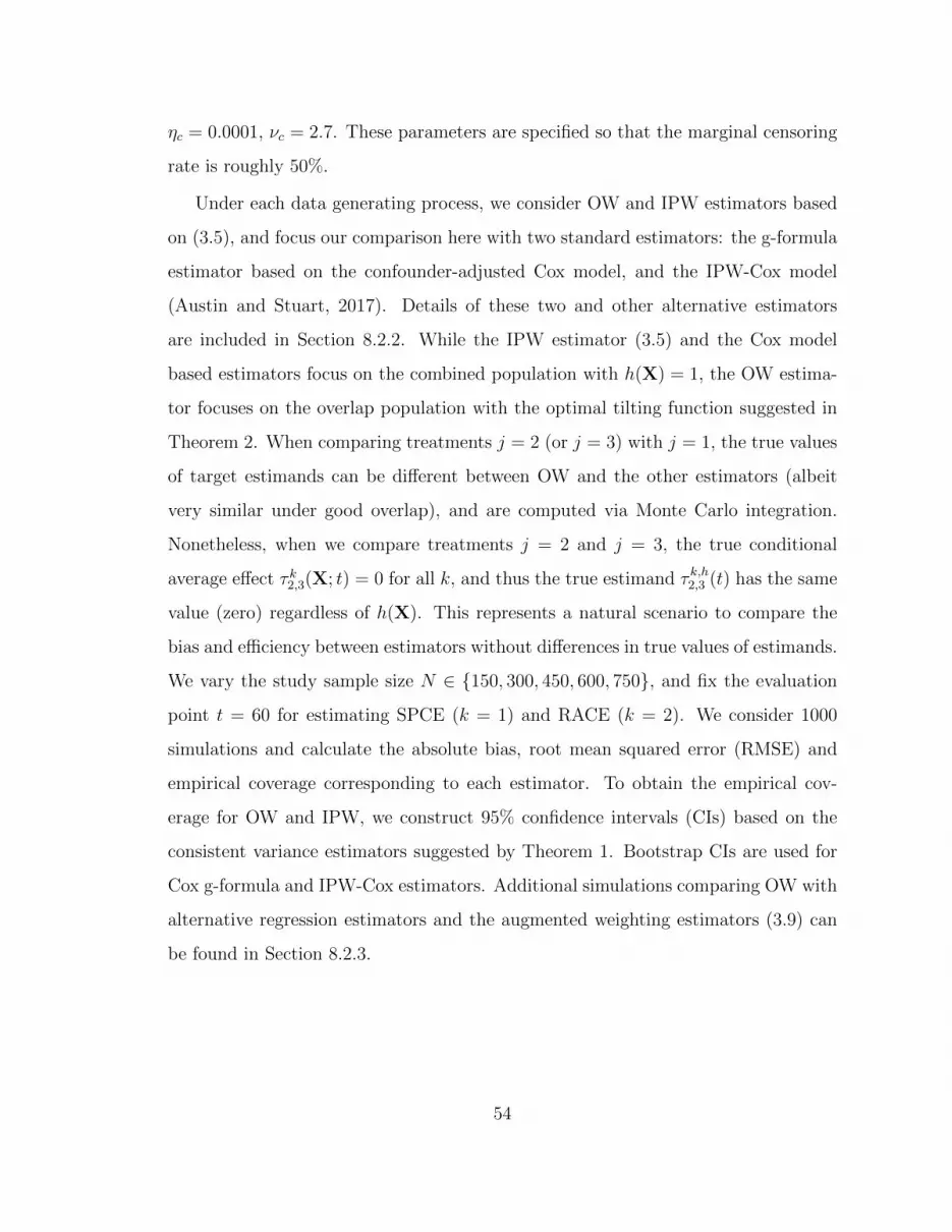
ηc = 0.0001, νc = 2.7. These parameters are specified so that the marginal censoring
rate is roughly 50%.
Under each data generating process, we consider OW and IPW estimators based
on (3.5), and focus our comparison here with two standard estimators: the g-formula
estimator based on the confounder-adjusted Cox model, and the IPW-Cox model
(Austin and Stuart, 2017). Details of these two and other alternative estimators
are included in Section 8.2.2. While the IPW estimator (3.5) and the Cox model
based estimators focus on the combined population with h(X) = 1, the OW estima-
tor focuses on the overlap population with the optimal tilting function suggested in
Theorem 2. When comparing treatments j = 2 (or j = 3) with j = 1, the true values
of target estimands can be different between OW and the other estimators (albeit
very similar under good overlap), and are computed via Monte Carlo integration.
Nonetheless, when we compare treatments j = 2 and j = 3, the true conditional
average effect τ k2,3(X; t) = 0 for all k, and thus the true estimand τ k,h2,3 (t) has the same
value (zero) regardless of h(X). This represents a natural scenario to compare the
bias and efficiency between estimators without differences in true values of estimands.
We vary the study sample size N ∈ 150, 300, 450, 600, 750, and fix the evaluation
point t = 60 for estimating SPCE (k = 1) and RACE (k = 2). We consider 1000
simulations and calculate the absolute bias, root mean squared error (RMSE) and
empirical coverage corresponding to each estimator. To obtain the empirical cov-
erage for OW and IPW, we construct 95% confidence intervals (CIs) based on the
consistent variance estimators suggested by Theorem 1. Bootstrap CIs are used for
Cox g-formula and IPW-Cox estimators. Additional simulations comparing OW with
alternative regression estimators and the augmented weighting estimators (3.9) can
be found in Section 8.2.3.
54

3.4.2 Simulation results
Under good overlap, Figure 8.5 presents the absolute bias, RMSE and coverage for
OW, IPW estimators based on (3.5), Cox g-formula as well as IPW-Cox estimators,
when survival outcomes are generated from model A and censoring is completely
independent. Here we focus on comparing treatment j = 2 versus j = 3, and thus
the true average causal effect among any target population is null. Across all three
estimands (SPCE, RACE and ASCE), OW consistently outperforms the IPW with
a smaller absolute bias and RMSE, and closer to nominal coverage across all levels
of N . Due to correctly specified outcome model, the Cox g-formula estimator is, as
expected, more efficient than the weighting estimators. However, its empirical cov-
erage is not always close to nominal, especially for estimating ASCE. The IPW-Cox
estimator has the largest bias, because the proportional hazards assumption does not
marginally among any of the target population. Figure 3.1 represents the counterpart
of Figure 8.4 but under poor overlap. The IPW estimator based on (3.5) is suscepti-
ble to lack of overlap due to extreme inverse probability weights, and has extremely
large bias, variance and low coverage. The bias and under-coverage remain for IPW
even after trimming units for whom maxjej(Xi) > 0.97 and minjej(Xi) < 0.03
(Figure 8.5). Under poor overlap, OW is more efficient than IPW regardless of trim-
ming, and becomes almost as efficient as the Cox g-formula estimator for estimating
RACE and ASCE. Furthermore, the proposed OW interval estimator consistently
carries close to nominal coverage for all three types of estimands. Figure 8.9 present
the counterparts of Figure 8.4 and Figure 3.1, but focus on comparing treatments
j = 2 and j = 1 where the true average causal effect is non-null. The patterns are
qualitatively similar.
In Table 3.1, we summarize the performance metrics for different estimators when
the proportional hazards assumption is violated and/or censoring depends on covari-
ates. Similar to Figure 3.1, we focus on comparing treatment j = 2 versus j = 3
such that the true average causal effect is null among any target population. When
55

200 300 400 500 600 700
0.00
0.04
0.08
0.12
SPCE
Sample size
BIA
S
200 300 400 500 600 7000
12
34
56
RACE
Sample size
BIA
S
200 300 400 500 600 700
02
46
810
ASCE
Sample size
BIA
S
200 300 400 500 600 700
0.05
0.10
0.15
SPCE
Sample size
RM
SE
200 300 400 500 600 700
23
45
67
8
RACE
Sample size
RM
SE
200 300 400 500 600 700
24
68
1012
14
ASCE
Sample sizeR
MS
E
200 300 400 500 600 700
0.6
0.7
0.8
0.9
1.0
SPCE
Sample size
CO
VE
R
200 300 400 500 600 700
0.7
0.8
0.9
1.0
RACE
Sample size
CO
VE
R
200 300 400 500 600 700
0.6
0.7
0.8
0.9
1.0
ASCE
Sample size
CO
VE
R
OW IPW Cox IPW−Cox
Figure 3.1: Absolute bias, root mean squared error (RMSE) and coverage for com-paring treatment j = 2 versus j = 3 under poor overlap, when survival outcomes aregenerated from model A and censoring is completely independent.
56

survival outcomes are generated from model B and hence the proportional hazards
assumption no longer holds, both the Cox g-formula and IPW-Cox estimators have
the largest bias, especially under poor overlap. In those scenarios, OW maintains the
largest efficiency, and consistently outperforms IPW in terms of bias and variance.
While the empirical coverage of IPW estimator deteriorates under poor overlap, the
coverage of OW estimator is robust to lack of overlap. When censoring further de-
pends on covariates, we modify the OW and IPW estimators using (3.8) where the
censoring survival functions are estimated by a Cox model. With the addition of in-
verse probability of censoring weights, only OW maintains the smallest bias, largest
efficiency and closest to nominal coverage under poor overlap across all types of esti-
mands. Results for comparing treatments j = 2 and j = 1 are similar and included
in Table 8.5.
In Section 8.2.3, we have additionally compared OW with alternative outcome
regression estimators similar to Mao et al. (2018), and the g-formula estimator based
on pseudo-observations (Andersen et al., 2017; Tanaka et al., 2020). These estimators
were originally developed with binary treatments, and we generalize them in Section
8.2.3 to multiple treatments for our purpose. Compared to OW estimator based on
(3.5), these alternative regression estimators are frequently less efficient and have
less than nominal coverage under poor overlap. An exception is the OW regression
estimator generalizing the work of Mao et al. (2018), which has similar performance
to the OW estimator based on (3.5). We have also carried out additional simulations
in Section 8.2.3 to examine the performance of augmented OW and IPW estimators
(3.9) relative to simple OW and IPW estimators (3.5). While including an outcome
regression component can notably improve the efficiency of IPW with survival out-
comes, the efficiency gain for OW estimator due to an additional outcome model is
somewhat limited, which favors the use of the OW estimator based on (3.5) due to
its simplicity. Finally, we replicate our simulations under a three-arm RCT similar to
Zeng et al. (2020d) (see Remark 3 and Section 8.2.3 for details). We confirmed that
57

Table 3.1: Absolute bias, root mean squared error (RMSE) and coverage for com-paring treatment j = 2 versus j = 3 under different degrees of overlap. In the“proportional hazards” scenario, the survival outcomes are generated from a Coxmodel (model A), and in the “non-proportional hazards” scenario, the survival out-comes are generated from an accelerated failure time model (model B). The samplesize is fixed at N = 300.
Degree of RMSE Absolute bias 95% Coverageoverlap OW IPW Cox IPW-Cox OW IPW Cox IPW-Cox OW IPW Cox IPW-Cox
Model A, completely random censoringSPCE Good 0.002 0.002 0.001 0.003 0.052 0.055 0.011 0.029 0.943 0.947 0.952 0.968
Poor 0.003 0.064 0.005 0.049 0.074 0.173 0.046 0.117 0.918 0.807 0.924 0.647
RACE Good 0.056 0.080 0.047 0.137 1.570 1.523 0.651 1.413 0.945 0.954 0.941 0.969Poor 0.106 2.817 0.252 3.151 2.523 5.784 2.709 6.093 0.931 0.812 0.963 0.650
ASCE Good 0.158 0.177 0.090 0.269 2.916 2.983 1.139 2.766 0.957 0.958 0.961 0.965Poor 0.213 5.433 0.490 4.930 4.305 12.131 4.750 11.625 0.935 0.791 0.749 0.658
Model B, completely random censoringSPCE Good 0.002 0.003 0.002 0.006 0.069 0.075 0.042 0.081 0.947 0.945 0.854 0.841
Poor 0.005 0.043 0.016 0.081 0.097 0.197 0.150 0.222 0.940 0.865 0.863 0.708
RACE Good 0.087 0.127 0.137 0.314 2.432 2.701 2.400 4.096 0.955 0.946 0.844 0.839Poor 0.111 2.962 0.947 4.646 3.862 7.330 8.653 11.275 0.935 0.853 0.830 0.709
ASCE Good 0.168 0.145 0.244 0.605 4.238 4.507 4.173 7.600 0.956 0.957 0.957 0.836Poor 0.223 4.307 1.661 7.562 6.274 13.157 15.027 20.920 0.941 0.862 0.731 0.702
Model A, conditionally independent censoringSPCE Good 0.001 0.002 0.001 0.000 0.044 0.048 0.039 0.039 0.955 0.946 0.906 0.963
Poor 0.005 0.047 0.009 0.089 0.060 0.154 0.056 0.149 0.910 0.792 0.871 0.641
RACE Good 0.003 0.005 0.065 0.022 2.257 2.094 2.315 1.717 0.950 0.949 0.929 0.964Poor 0.168 3.167 0.532 4.603 2.974 6.264 3.334 7.159 0.936 0.858 0.900 0.635
ASCE Good 0.008 0.276 0.163 0.188 4.447 9.351 4.899 10.564 0.952 0.950 0.950 0.974Poor 0.110 10.523 1.032 11.657 9.557 22.308 7.157 43.651 0.929 0.768 0.739 0.773
Model B, conditionally independent censoringSPCE Good 0.000 0.001 0.001 0.000 0.037 0.055 0.055 0.059 0.952 0.906 0.772 0.902
Poor 0.002 0.007 0.012 0.025 0.052 0.056 0.164 0.082 0.925 0.879 0.803 0.899
RACE Good 0.005 0.003 0.064 0.136 4.733 4.738 2.944 5.310 0.951 0.953 0.794 0.855Poor 0.132 0.573 0.712 1.594 6.655 6.546 9.092 7.515 0.954 0.899 0.775 0.845
ASCE Good 0.004 0.055 0.166 0.268 4.436 4.265 4.761 6.548 0.951 0.953 0.937 0.852Poor 0.179 0.428 1.339 1.973 6.516 7.589 13.039 8.835 0.957 0.908 0.747 0.846
58

OW and IPW estimators based on (3.5) are valid for covariate adjustment in RCTs
since they lead to substantially improved efficiency over the unadjusted comparisons
of pseudo-observations.
3.5 Application to National Cancer Database
We illustrate the proposed weighting estimators by comparing three treatment op-
tions for prostate cancer in an observational dataset with 44,551 high-risk, localized
prostate cancer patients drawn from the National Cancer Database (NCDB). These
patients were diagnosed between 2004 and 2013, and either underwent a surgical
procedure – radical prostatectomy (RP), or were treated by one of two therapeu-
tic procedures – external beam radiotherapy combined with androgen deprivation
(EBRT+AD) or external beam radiotherapy plus brachytherapy with or without an-
drogen deprivation (EBRT+brachy±AD). We focus on time to death since treatment
initiation as the primary outcome, and pre-treatment confounders include age, clin-
ical T stage, Charlson-Deyo score, biopsy Gleason score, prostate-specific antigen
(PSA), year of diagnosis, insurance status, median income level, education, race, and
ethnicity. A total of 2,434 patients died during the study period with their survival
outcome observed, while other patients have right-censored outcomes. The median
and maximum follow-up time is 21 and 115 months, respectively.
We used a multinomial logistic model to estimate the generalized propensity
scores, and visualized the distribution of estimated scores in Figure 8.11. We model
age and PSA by natural splines as in Ennis et al. (2018), and keep linear terms for
all other covariates. We found good overlap across groups regarding the propen-
sity of receiving EBRT+brachy±AD, but a slight lack of overlap regarding the
propensity of receiving RP and EBRT+AD. We checked the weighted covariate
balance under IPW and OW based on the maximum pairwise absolute standard-
ized difference (MPASD) criteria, and present the balance statistics in Table 8.6.
The MPASD for the pth covariate is defined as maxj<j′|Xp,j − Xp,j′|/Sp, where
59

Xp,j =∑N
i=1 1Zi = jXi,pwhj (Xi)/
∑Ni=1 1Zi = jwhj (Xi) is the weighted covariate
mean in group j, and S2p = J−1
∑Jj=1 S
2p,j is the unweighted sample variance averaged
across all groups. Both IPW and OW improved covariate balance, with OW leading
to consistently smaller MPASD, whose value is below the usual 0.1 threshold for all
covariates.
Figure 3.2 presents the estimated causal survival curves for each treatment, Eh(X)
1Ti(j) ≥ t/E(h(X)), along with the 95% confidence bands in the combined pop-
ulation (corresponding to IPW) and the overlap population (corresponding to OW).
We chose 220 grid points equally spaced by half a month for this evaluation. The
estimated causal survival curves among the two target populations are generally sim-
ilar, which is expected given there is only a slight lack of overlap (Figure 8.11).
The surgical treatment, RP, shows the largest survival benefit, followed by the ra-
diotherapeutic treatment, EBRT+brachy±AD, while EBRT+AD results in the worst
survival outcomes during the first 80 months or so. Importantly, the estimated causal
survival curves for the RP and EBRT+brachy±AD crossed after month 80, suggest-
ing potential violations to the proportional hazards assumption commonly assumed
in survival analysis. Figure 3.3a and 3.3b further characterized the the SPCE and
RACE as a function of time t with the associated 95% confidence bands. Evidently,
the SPCE results confirmed the largest causal survival benefit due to RP, followed by
EBRT+brachy±AD. The associated confidence band of SPCE from OW is narrower
than that from IPW and frequently excludes zero. While the analysis of the pairwise
RACE yielded similar findings, the efficiency of OW over IPW became more relevant
when comparing RP and EBRT+brachy±AD. Specifically, the confidence band of
RACE from OW excludes zero until month 80, while the confidence band of RACE
from IPW straddles zero across the entire follow-up period. This analysis shed new
light on the significant causal survival benefit of RP over EBRT+brachy±AD at the
0.05 level in terms of the restricted mean survival time, which was not identified in
previous analysis (Ennis et al., 2018).
60

0.4
0.6
0.8
1.0
0 30 60 90Months after treatment
Sur
viva
l Pro
b, a
djus
ted
by IP
WEBRT+AD
EBRT+brachy±AD
RP
0.4
0.6
0.8
1.0
0 30 60 90Months after treatment
Sur
viva
l Pro
b, a
djus
ted
by O
W
Figure 3.2: Survival curves of the three treatments of prostate cancer (Section 3.5)estimated from the pseudo-observations-based weighting estimator, using IPW (left)and OW (right).
−0.3
−0.2
−0.1
0.0
0.1
0 30 60 90Months after treatment
EB
RT
+A
D v
s R
P C
ompa
rison
, SP
CE
Method
IPW
OW
−0.25
0.00
0.25
0 30 60 90Months after treatment
EB
RT
+br
achy
±AD
vs
RP
Com
paris
on, S
PC
E
−0.2
0.0
0.2
0.4
0 30 60 90Months after treatment
EB
RT
+br
achy
±AD
vs
EB
RT
+A
D C
ompa
rison
, SP
CE
(a) Estimated survival probability as a function of time t in three treatment groups.
−10.0
−7.5
−5.0
−2.5
0.0
0 30 60 90Months after treatment
EB
RT
+A
D v
s R
P C
ompa
rison
, RA
CE
Method
IPW
OW
−3
0
3
6
0 30 60 90Months after treatment
EB
RT
+br
achy
±AD
vs
RP
Com
paris
on, R
AC
E
0.0
2.5
5.0
7.5
10.0
0 30 60 90Months after treatment
EB
RT
+br
achy
±AD
vs
EB
RT
+A
D C
ompa
rison
, RA
CE
(b) Estimated restricted mean survival time as a function of time t in three treat-ment groups.
Figure 3.3: Point estimates and 95% confidence bands of SPCE and RACE as afunction of time from the pseudo-observations-based IPW and OW estimator in theprostate cancer application in Section 3.5.
61

In Table 3.2, we also reported the SPCE and RACE using the IPW and OW
estimators, as well as the Cox g-formula and IPW-Cox estimators at t = 60 months,
i.e. the 80th quantile of the follow-up time. All methods conclude that RP leads to
significantly lower mortality rate at 60 months than EBRT+AD. Compared to IPW,
OW provides similar point estimates and no larger variance estimates. Consistently
with Figure 3.3b, the smaller variance estimate due to OW (compared to IPW) leads
to a change in conclusion when comparing EBRT+brachy±AD versus RP in terms of
RACE at the 0.05 level and confirms the significant treatment benefit of RP. The Cox
g-formula and IPW-Cox estimators sometimes provide considerably different results
than weighting estimators based on (3.5), as they assumed proportional hazards which
may not hold. Overall, we found that, compared to RP, the two radiotherapeutic
treatments led to a shorter restricted mean survival time (1.2 months shorter with
EBRT+AD and 0.5 month shorter with EBRT+brachy±AD) up to five years after
treatment. The 5-year survival probability is also 6.7% lower under EBRT+AD and
3.1% lower under EBRT+brachy±AD compared to RP.
62

Table 3.2: Pairwise treatment effect estimates of the three treatments of prostatecancer (Section 3.5) using four methods, on the scale of restricted average causaleffect (RACE) and survival probability causal effect (SPCE) at 60 months/5 yearspost-treatment.
Method Estimate Standard error 95% Confidence interval p-valueEBRT-AD vs. RP comparisonRestricted average causal effect
OW -1.277 0.150 (-1.524, -1.031) 0.000IPW -0.917 0.264 (-1.351, -0.484) 0.001COX -1.342 0.126 (-1.549, -1.136) 0.000MSM -0.931 0.220 (-1.294, -0.568) 0.000
Survival probability causal effectOW -0.062 0.009 (-0.076, -0.048) 0.000IPW -0.067 0.009 (-0.083, -0.052) 0.000COX -0.059 0.006 (-0.068, -0.050) 0.000MSM -0.039 0.010 (-0.056, -0.023) 0.000
EBRT+brachy±AD vs. RP comparisonRestricted average causal effect
OW -0.562 0.236 (-0.950, -0.174) 0.017IPW -0.309 0.331 (-0.855, 0.236) 0.350COX -0.802 0.214 (-1.155, -0.450) 0.000MSM -0.363 0.317 (-0.885, 0.158) 0.252
Survival probability causal effectOW -0.032 0.013 (-0.054, -0.010) 0.016IPW -0.031 0.013 (-0.053, -0.009) 0.021COX -0.036 0.009 (-0.051, -0.020) 0.000MSM -0.015 0.014 (-0.038, 0.007) 0.256
EBRT+brachy±AD vs. EBRT+AD comparisonRestricted average causal effect
OW 0.715 0.240 (0.321, 1.109) 0.003IPW 0.710 0.242 (0.195, 1.021) 0.015COX 0.540 0.216 (0.184, 0.896) 0.012MSM 0.568 0.246 (0.163, 0.973) 0.021
Survival probability causal effectOW 0.030 0.014 (0.006, 0.053) 0.036IPW 0.036 0.014 (0.013, 0.059) 0.011COX 0.024 0.009 (0.008, 0.039) 0.013MSM 0.024 0.010 (0.007, 0.041) 0.021
63

4
Mediation analysis with sparse and irregularlongitudinal data
4.1 Introduction
Mediation analysis seeks to understand the role of an intermediate variable (i.e. me-
diator) M that lies on the causal path between an exposure or treatment Z and an
outcome Y . The most widely used mediation analysis method, proposed by Baron
and Kenny (1986), fits two linear structural equation models (SEMs) between the
three variables and interprets the model coefficients as causal effects. There is a vast
literature on the Baron-Kenny framework across a variety of disciplines, including
psychology, sociology, and epidemiology (see MacKinnon, 2012). A major advance-
ment in recent years is the incorporation of the potential-outcome-based causal in-
ference approach (Neyman, 1990; Rubin, 1974). This led to a formal definition of
relevant causal estimands, clarification of identification assumptions, and new esti-
mation strategies beyond linear SEMs (Robins and Greenland, 1992; Pearl, 2001; So-
bel, 2008; Tchetgen Tchetgen and Shpitser, 2012; Daniels et al., 2012; VanderWeele,
2016). In particular, Imai et al. (2010b) proved that the Baron-Kenny estimator
can be interpreted as a special case of a causal mediation estimator given additional
assumptions. These methodological advancements opened up new application ar-
eas including imaging, neuroscience, and environmental health (Lindquist and Sobel,
2011; Lindquist, 2012; Zigler et al., 2012; Kim et al., 2019). Comprehensive reviews
on causal mediation analysis are given in VanderWeele (2015); Nguyen et al. (2020).
In the traditional settings of mediation analysis, exposure Z, mediation M and
outcome Y are all univariate variables at a single time point. Recent work has
64

extended to time-varying cases, where at least one of the triplet (Z,M, Y ) is lon-
gitudinal. This line of research has primarily focused on cases with time-varying
mediators or outcomes that are observed on sparse and regular time grids (van der
Laan and Petersen, 2008; Roth and MacKinnon, 2012; Lin et al., 2017a). For exam-
ple, VanderWeele and Tchetgen Tchetgen (2017) developed a method for identify-
ing and estimating causal mediation effects with time-varying exposures and medi-
ators based on marginal structural models (Robins et al., 2000a). Some researchers
also investigated the case with time-varying exposure and mediator for the survival
outcome (Zheng and van der Laan (2017); Lin et al. (2017b)). Another stream of
research, motivated by applications in neuroimaging, focuses on cases where media-
tors or outcomes are densely recorded continuous functions, e.g. the blood-oxygen-
level-dependent (BOLD) signal collected in a functional magnetic resonance imaging
(fMRI) session. In particular, Lindquist (2012) introduced the concept of functional
mediation in the presence of a functional mediator and extended causal SEMs to
functional data analysis (Ramsay and Silverman, 2005). Zhao et al. (2018) further
extended this approach to functional exposure, mediator and outcome.
Sparse and irregularly-spaced longitudinal data are increasingly available for causal
studies. For example, in electronic health records (EHR) data, the number of ob-
servations usually varies between patients and the time grids are uneven. The same
situation applies in animal behavior studies due to the inherent difficulties in observ-
ing wild animals. Such data structure poses challenges to existing causal mediation
methods. First, one cannot simply treat the trajectories of mediators and outcomes
as functions as in Lindquist (2012) because the sparse observations render the tra-
jectories volatile and non-smooth. Second, with irregular time grids the dependence
between consecutive observations changes over time, making the methods based on
sparse and regular longitudinal data such as VanderWeele and Tchetgen Tchetgen
(2017) not applicable. A further complication arises when the mediator and outcome
are measured with different frequencies even within the same individual.
65

In this chapter, we propose a causal mediation analysis method for sparse and
irregular longitudinal data that address the aforementioned challenges. Similar to
Lindquist (2012) and Zhao et al. (2018), we adopt a functional data analysis per-
spective (Ramsay and Silverman, 2005), viewing the sparse and irregular longitudi-
nal data as realizations of underlying smooth stochastic processes. We define causal
estimands of direct and indirect effects accordingly and provide assumptions for non-
parametric identification (Section 4.3). For estimation and inference, we proceed
under the classical two-SEM mediation framework (Imai et al., 2010b) but diverge
from the existing methods in modeling (Section 4.4). Specifically, we employ the func-
tional principal component analysis (FPCA) approach (Yao et al., 2005; Jiang and
Wang, 2010, 2011; Han et al., 2018) to project the mediator and outcome trajectories
to a low-dimensional representation. We then use the first few functional principal
components (instead of the whole trajectories) as predictors in the structural equa-
tion models. To accurately quantify the uncertainties, we employ a Bayesian FPCA
model (Kowal and Bourgeois, 2020) to simultaneously estimate the functional princi-
pal components and the structural equation models. Though the Bayesian approach
to mediation analysis has been discussed before (Daniels et al., 2012; Kim et al., 2017,
2018), it has not been developed for the setting of sparse and irregular longitudinal
data.
Our motivating application is the evaluation of the causal relationships between
early adversity, social bonds, and physiological stress in wild baboons (Section 4.2).
Here the exposure is early adversity (e.g. drought, maternal death before reaching
maturity), the mediators are the strength of adult social bonds, and the outcomes
are adult glucocorticoid (GC) hormone concentrations, which is a measure of an
animal’s physiological stress level. The exposure, early adversity, is a binary variable
measured at one time point, whereas both the mediators and outcomes are sparse
and irregular longitudinal variables. We apply the proposed method to a prospective
and longitudinal observational data set from the Amboseli Baboon Research Project
66

located in the Amboseli ecosystem, Kenya (Alberts and Altmann, 2012) (Section
4.5). We find that experiencing one or more sources of early adversity leads to
significant direct effects (a 9-14% increase) on females’ GC concentrations across
adulthood, but find little evidence that these effects were mediated by weak social
bonds. Though motivated from a specific application, the proposed method is readily
applicable to other causal mediation studies with similar data structure, including
EHR and ecology studies. Furthermore, our method is also applicable to regularly
spaced longitudinal observations.
4.2 Motivating application: early adversity, social bond and stress
4.2.1 Biological background
Conditions in early life can have profound consequences for individual development,
behavior, and physiology across the life course (Lindstrom, 1999; Gluckman et al.,
2008; Bateson et al., 2004). These early life effects are important, in part, because
they have major implications for human health. One leading explanation for how
early life environments affect adult health is provided by the biological embedding
hypothesis, which posits that early life stress causes developmental changes that cre-
ate a “pro-inflammatory” phenotype and elevated risk for several diseases of aging
(Miller et al., 2011). The biological embedding hypothesis proposes at least two,
non-exclusive causal pathways that connect early adversity to poor health in adult-
hood. In the first pathway, early adversity leads to altered hormonal profiles that
contribute to downstream inflammation and disease. Under this scenario, stress in
early life leads to dysregulation of hormonal signals in the body’s main stress re-
sponse system, leading to the release of GC hormone, which engages the body’s
fight-or-flight response. Chronic activation is associated with inflammation and ele-
vated disease risk (McEwen, 1998; Miller et al., 2002; McEwen, 2008). In the second
causal pathway, early adversity hampers an individual’s ability to form strong inter-
personal relationships. Under this scenario, the social isolation contributes to both
67

altered GC profiles and inflammation.
Hence, the biological embedding hypothesis posits that early life adversity affects
both GC profiles and social relationships in adulthood, and that poor social relation-
ships partly mediate the connection between early adversity and GCs. Importantly,
the second causal pathway—mediated through adult social relationships—suggests
an opportunity to transmit the negative health effect of early adversity. Specifically,
strong and supportive social relationships may dampen the stress response or reduce
individual exposure to stressful events, which in turn reduces GCs and inflamma-
tion. For example, strong and supportive social relationships have repeatedly been
linked to reduced morbidity and mortality in humans and other social animals (Holt-
Lunstad et al., 2010; Silk, 2007). In addition to the biological embedding hypothesis,
this idea of social mediation is central to several hypotheses that propose causal con-
nections between adult social relationships and adult health, even independent of
early life adversity; these hypotheses include the stress buffering and stress preven-
tion hypotheses (Cohen and Wills, 1985; Landerman et al., 1989; Thorsteinsson and
James, 1999) and the social causation hypothesis (Marmot et al., 1991; Anderson
and Marmot, 2011).
Despite the aforementioned research, the causal relationships among early ad-
versity, adult social relationships, and HPA (hypothalamic–pituitary–adrenal) axis
dysregulation remain the subject of considerable debate. While social relationships
might exert direct effects on stress and health, it is also possible that poor health and
high stress limit an individual’s ability to form strong and supportive relationships.
As such, the causal arrow flows backwards, from stress to social relationships (Case
and Paxson, 2011). In another causal scenario, early adversity exerts independent
effects on social relationships and the HPA axis, and correlations between social re-
lationships and GCs are spurious, arising solely as a result of their independent links
to early adversity (Marmot et al., 1991).
68

4.2.2 Data
In this chapter, we test whether the links between early adversity, the strength of
adult social bonds, and GCs are consistent with predictions derived from the biolog-
ical embedding hypothesis and other related theories. Specifically, we use data from
a well-studied population of savannah baboons in the Amboseli ecosystem in Kenya.
Founded in 1971, the Amboseli Baboon Research Project has prospective longitudi-
nal data on early life experiences, and fine-grained longitudinal data on adult social
bonds and GC hormone concentrations, a measure of the physiological stress response
(Alberts and Altmann, 2012).
Our study sample includes 192 female baboons. Each baboon entered the study
after becoming mature at age 5, and we had information on its experience of six
sources of early adversity (i.e., exposure) (Tung et al., 2016; Zipple et al., 2019):
drought, maternal death, competing sibling, high group density, low maternal rank,
and maternal social isolation. Table 4.1 presents the number of baboons that ex-
perienced each early adversity. Overall, while only a small proportion of subjects
experienced any given source of early adversity, most subjects experienced at least
one source of early adversity. Therefore, in our analysis we also create a cumulative
exposure variable that summarizes whether a baboon experienced any source of the
adversity.
Table 4.1: Sources of early adversity and the number of baboons experienced eachtype of early adversity. The last row summarizes the number of baboons had at leastone of six individual adversity sources.
early adversity no. subjects did not experience no. subjects did experience(control) (exposure)
Drought 164 28Competing Sibling 153 39High group density 161 31Maternal death 157 35Low maternal rank 152 40Maternal Social isolation 140 52At least one 48 144
69

Each baboon’s adult social bonds (i.e. mediators) and fecal GC hormone concen-
trations (i.e. outcomes) are measured repeatedly throughout its life on the same grid.
Social bonds are measured using the dyadic sociality index with females (DSI-F) (Silk
et al., 2006). The indices are calculated for each female baboon separately based on
all visible observations for social interactions between the baboon and other members
in the entire social group within a given period. Larger values mean stronger social
bonds. We normalized the DSI-F measurements, and the normalized DSI-F values
range from −1.47 to 3.31 with mean value at 1.04 and standard deviation 0.51. The
fecal GC concentrations were collected opportunistically, and the values range from
7.51 to 982.87 with mean 74.13 and standard deviation 38.25. Age is used to index
within-individual observations on both social bond and GC concentrations. Only
about 20% baboons survive until age 18 and thus data on females older than 18
years are extremely sparse and volatile. Therefore, we truncated all trajectories at
age 18, resulting in a final sample with 192 female baboons and 9878 observations.
For wild animals, the observations usually made on irregular or opportunistic
basis. We have on average 51.4 observations of each baboon for both social bonds and
GC concentrations, but the number of observations of a single baboon ranges from 3
to 113. Figure 4.1 shows the mediator and outcome trajectories as a function of age
of two randomly selected baboons in the sample. We can see that the frequency of the
observations and time grids of the mediator or outcome trajectories vary significantly
between baboons.
We also have a set of static and time-varying covariates that are deemed important
to wild baboons’s physiology and behavior. These include reproductive state (i.e.
cycling, pregnant, or lactating), density of the social group, max temperature in the
last 30 days before the fecal sample was collected, whether the sample is collected in
wet or dry season, the amount of rainfall, relative dominance rank of a baboon, and
number of coresident adult maternal relatives.More information on the covariates,
exposure, mediator, and outcomes can be found in Rosenbaum et al. (2020).
70
0.5
2
Mediator, baboon 1
2010
0
Outcome, baboon 1
01.
5Mediator, baboon 2
Age at sample collection
5010
015
0
Outcome, baboon 2
Figure 4.1: Observed trajectories of social bonds and GC hormone as a functionof age of two randomly selected female baboons in the study sample.
4.3 Causal mediation framework
4.3.1 Setup and causal estimands
Suppose we have a sample of N units (in the use case described here, baboons); each
unit i (i = 1, 2, · · · , N) is assigned to a treatment (Zi = 1) or a control (Zi = 0) group.
For each unit i, we make observations at Ti different time points tij ∈ [0, T ], j =
1, 2, · · · , Ti, and Ti can vary between units. At each time point tij, we measure an
outcome Yij and a mediator Mij prior to the outcome, and a vector of p time-varying
covariates Xij = (Xij,1, · · · , Xij,p)′. For each unit, the observations points are sparse
along the time span and irregularly spaced. For simplicity, we assume the observed
time grids for the outcome and the mediator are the same within one unit. However,
our method is directly applicable when the observation grids for the outcome and the
mediator are different for a given individual.
A key to our method is to view the observed mediator and outcome values drawn
from a smooth underlying process Mi(t) and Yi(t), t ∈ [0, T ], with Normal measure-
71

ment errors, respectively:
Mij = Mi(tij) + εij, εij ∼ N (0, σ2m), (4.1)
Yij = Yi(tij) + νij, νij ∼ N (0, σ2y). (4.2)
Hence, instead of directly exploring the relationship between the treatment Zi, me-
diators Mij and outcomes Yij, we investigate the relationship between Zi and the
stochastic processes Mi(tij) and Yi(tij). In particular, we wish to answer two ques-
tions: (a) how big is the causal impact of the treatment on the outcome process, and
(b) how much of that impact is mediated through the mediator process?
To be consistent with the standard notation of potential outcomes in causal infer-
ence (Imbens and Rubin, 2015), from now on we move the time index of the mediator
and outcome process to the superscript: Mi(t) = M ti , Yi(t) = Y t
i . Also, we use the
following bold font notation to represent a process until time t: Mti ≡ M s
i , s ≤ t ∈
R[0,t], and Yti ≡ Y s
i , s ≤ t ∈ R[0,t]. Similarly, we denote covariates between the jth
and j + 1th time point for unit i as Xti = Xi1, Xi2, · · · , Xij′ for tij′ ≤ t < tij′+1.
We extend the definition of potential outcomes to define the causal estimands.
Specifically, let Mti(z) ∈ R[0,t] for z = 0, 1, t ∈ [0, T ], denote the potential values of
the underlying mediator process for unit i until time t under the treatment status
z; let Yti(z,m) ∈ R[0,t] be the potential outcome for unit i until time t under the
treatment status z and the mediator process taking value of Mti = m with m ∈ R[0,t].
The above notation implicitly makes the stable unit treatment value assumption
(SUTVA) (Rubin, 1980), which states that (i) there is no different version of the
treatment, and (ii) there is no interference between the units, more specifically, the
potential outcomes of one unit do not depend on the treatment and mediator values
of other units. SUTVA is plausible in our application. First, there is unlikely different
versions of the early adversities. Second, though baboons live in social groups, it is
unlikely a baboon’s long-term GC concentration (outcome) was much affected by
the early adversities experienced by other cohabitant baboons in its social group,
72

particularly considering the fact that only a small proportion of baboons experienced
any given early adversity. Moreover, the social bond index (mediator) summarizes
the interaction between a focal baboon and other members in a social group, and thus
we can view the impact from other baboons as constant while examining the variation
of social bond for the focal baboon. The notation of Yti(z,m) makes another implicit
assumption that the potential outcomes are determined by the mediator values m
before time t, but not after t. For each unit, we can only observe one realization from
the potential mediator or outcome process:
Mti = Mt
i(Zi) = ZiMti(1) + (1− Zi)Mt
i(0), (4.3)
Yti = Yt
i(z,Mti(Zi)) = ZiY
ti(1,M
ti(1)) + (1− Zi)Yt
i(0,Mti(0)). (4.4)
We define the total effect (TE) of the treatment Zi on the outcome process at
time t as:
τ tTE = EY ti (1,Mt
i(1))− Y ti (0,Mt
i(0)). (4.5)
When there is a mediator, the TE can be decomposed into direct and indirect effects.
Below we extend the framework of Imai et al. (2010b) to formally define these effects.
First, we define the average causal mediation (or indirect) effect (ACME) under
treatment z at time t by fixing the treatment status while altering the mediator
process:
τ tACME(z) ≡ EY ti (z,Mt
i(1))− Y ti (z,Mt
i(0)), z = 0, 1. (4.6)
The ACME quantifies the difference between the potential outcomes, given a fixed
treatment status z, corresponding to the potential mediator process under treatment
Mti(1) and that under control Mt
i(0). In the previous literature, variants of the
ACME are also called the natural indirect effect (Pearl, 2001), or the pure indirect
effect for τ tACME(0) and total indirect effect for τ tACME(1) (Robins and Greenland, 1992)
Second, we define the average natural direct effect (ANDE) (Pearl, 2001; Imai
et al., 2010b) of treatment on the outcome at time t by fixing the mediator process
73

while altering the treatment status:
τ tANDE(z) ≡ EY ti (1,Mt
i(z))− Y ti (0,Mt
i(z)). (4.7)
The ANDE quantifies the portion in the TE that does not pass through the mediators.
It is easy to verify that the TE is the sum of ACME and ANDE:
τ tTE = τ tACME(z) + τ tANDE(1− z), z = 0, 1. (4.8)
This implies we only need to identify two of the three quantities τTE, τ tACME(z),
τ tANDE(z). In this chapter, we will focus on the estimation of τTE and τ tACME(z). Because
we only observe a portion of all the potential outcomes, we cannot directly identify
these estimands from the observed data, which would require additional assumptions.
4.3.2 Identification assumptions
In this subsection, we list the causal assumptions necessary for identifying the ACME
and ANDEs with sparse and irregular longitudinal data. There are several sets of
identification assumptions in the literature (Robins and Greenland, 1992; Pearl, 2001;
Imai et al., 2010a; Shpitser and VanderWeele, 2011) with subtle distinction (Ten Have
and Joffe, 2012). Here we follow the similar set of assumptions in Imai et al. (2010b)
and Forastiere et al. (2018).
The first assumption extends the standard ignorability assumption and rules out
the unmeasured treatment-outcome confounding.
Assumption 1 (Ignorability). Conditional on the observed covariates, the treatment
is unconfounded with respect to the potential mediator process and the potential out-
comes process:
Yti(1,m),Yt
i(0,m),Mti(1),Mt
i(0) ⊥⊥ Zi | Xti,
for any t and m ∈ R[0,t].
74

In our context, Assumption 1 indicates that there is no unmeasured confounding,
besides the observed covariates, between the sources of early adversity and the pro-
cesses of social bonds and GCs. In other words, early adversity is randomized among
the baboons with the same covariates. This assumption is plausible given the early
adversity events considered in this study are largely imposed by nature.
The second assumption extending the sequential ignorability assumption in Imai
et al. (2010b); Forastiere et al. (2018) to the functional data setting.
Assumption 2 (Sequential Ignorability). There exists ε > 0, such that for any
0 < ∆ < ε,the increment of the mediator process is independent of the increment of
potential outcomes process from time t to t+∆, conditional on the observed treatment
status, covariates and the mediator process up to time t:
Y t+∆i (z,m)− Y t
i (z,m) ⊥⊥ M t+∆i (z′)−M t
i (z′) | Zi,Xt
i,Mti(z′′),
for any z, z′, z′′, 0 < ∆ < ε, t, t+ ∆ ∈ [0, T ],m ∈ R[0,T ].
In our application, Assumption 2 implies that conditioning on the early adversity
status, covariates, and the potential social bond history up to a given time point,
any change in the social bond values within a sufficiently small time interval ∆ is
randomized with respect to the change in the potential outcomes. Namely, there are
no unobserved mediator-outcomes confounders in a sufficiently small time interval.
Though it differs in the specific form, Assumption 2 is in essence the same sequential
ignorability assumption used for the regularly spaced observations in Bind et al.
(2015) and VanderWeele and Tchetgen Tchetgen (2017). This is a crucial assumption
in mediation analysis, but is strong and generally untestable in practice because it is
usually impossible to manipulate the mediator values, even in randomized trials.
Assumptions 1 and 2 are illustrated by the directed acyclic graphs (DAG) in Fig-
ure 4.2a, which condition on the covariates Xti and a window between two sufficiently
close time points t and t + ∆. The arrows between Zi, Mti , Y
ti represent a causal
75

relationship (i.e., nonparametric structural equation model), with solid and dashed
lines representing measured and unmeasured relationships, respectively. Figure 4.2b
and 4.2c depicts two possible scenarios where Assumptions 1 and 2 are violated,
respectively, where Ui represents an unmeasured confounder.
Zi ...M ti M t+∆
i
...Y ti Y t+∆
i
(a) DAG of Assumption 1 and 2
Zi ...Mi(t) Mi(t+ ∆)
...Yi(t) Yi(t+ ∆)Ui
Zi ...Mi(t) Mi(t+ ∆)
...Yi(t) Yi(t+ ∆)Ui
(b) DAG of two examples of violation to Assumption 1 (ignorability)
Zi ...Mi(t) Mi(t+ ∆)
...Yi(t) Yi(t+ ∆)
Ui
Zi ...Mi(t) Mi(t+ ∆)
...Yi(t) Yi(t+ ∆)
(c) DAG of two examples of violation to Assumption 2 (sequential ignorability)
Figure 4.2: Directed acyclic graphs (DAG) of Assumptions1,2 and examples ofpossible violations. The arrows between variables represent a causal relationship,with solid and dashed lines representing measured and unmeasured relationships,respectively.
Assumptions 1 and 2 allow nonparametric identification of the TE and ACME
from the observed data, as summarized in the following theorem.
Theorem 3. Under Assumption 1,2, and some regularity conditions (specified in the
Section 8.3.1), the TE, ACME and ANDE can be identified nonparametrically from
76

the observed data: for z = 0, 1, we have
τTE =
∫X
E(Y ti |Zi = 1,Xt
i = xt)− E(Y ti |Zi = 0,Xt
i = xt)dFXti(xt),
τ tACME(z) =
∫X
∫R[0,t]
E(Y ti |Zi = z,Xt
i = xt,Mti = m)dFXt
i(xt)×
dFMti|Zi=1,Xt
i=xt(m)− FMti|Zi=0,Xt
i=xt(m),
where FW (·) and FW |V (·) denotes the cumulative distribution of a random variable or
a vector W and the conditional distribution given another random variable or vector
V , respectively.
The proof of Theorem 3 is provided in the Section 8.3.1. Theorem 3 implies that
estimating the causal effects requires modeling two components: (a) the conditional
expectation of observed outcome process given the treatment, covariates, and the
observed mediator process, E(Y ti |Zi,Xt
i,Mti), and (b) the distribution of the observed
mediator process given the treatment and the covariates, FMti|Zi,Xt
i(·). These two
components correspond to the two linear structural equations in the classic mediation
framework of Baron and Kenny (1986). In the setting of functional data, we can
employ more flexible models instead of linear regression models, and express the TE
and ACME as functions of the model parameters. Theorem 3 can be readily extended
to more general scenarios such as discrete (i.e., as opposed to continuous) mediators
and time-to-event outcomes.
4.4 Modeling mediator and outcome via functional principal compo-nent analysis
In this section, we propose to employ the functional principal component analysis
(FPCA) approach to infer the mediator and outcome processes from sparse and
irregular observations (Yao et al., 2005; Jiang and Wang, 2010, 2011). In order to take
into account the uncertainty due to estimating the functional principal components
(Goldsmith et al., 2013), we adopt a Bayesian model to jointly estimate the principal
77

components and the structural equation models. Specifically, we impose a Bayesian
FPCA model similar to that in Kowal and Bourgeois (2020) to project the observed
mediator and outcome processes into lower-dimensional representations and then
take the first few dominant principal components as the predictors in the structural
equation models.
We assume the potential processes for mediators Mti(z) and outcomes Yt
i(z,m)
have the following Karhunen-Loeve decomposition,
M ti (z) = µM(Xt
i) +∞∑r=1
ζri,zψr(t), (4.9)
Y ti (z,m) = µY (Xt
i) +
∫ t
0
γ(s, t)m(s)ds+∞∑s=1
θsi,zηs(t). (4.10)
where µM(·) and µY (·) are the mean functions of the mediator process Mti and out-
come process Yti , respectively; ψr(t) and ηs(t) are the Normal orthogonal eigenfunc-
tions for Mti and Yt
i , respectively, and ζri,z and θsi,z are the corresponding principal
scores of unit i. The above model assumes that the treatment affects the mediation
and the outcome processes only through the principal scores. We represent the medi-
ator and outcome process of each unit with its principal score ζri,z and θsi,z. Given the
principal scores , we can transform back to the smooth process with a linear combi-
nation. As such, if we are interested in the differences in the process, it is equivalent
to investigate the difference in the principal scores. Also, as we usually require only
3 or 4 components to explain most of the variation, we reduce the dimensions of
the trajectories effectively by projecting the difference to the principal scores. With
the model specification in (4.10), we make an implicit assumption that the ACME
and ANDE are the same in the treatment and control groups in our application,
τ tACME(0) = τ tACME(1), τ tANDE(0) = τ tANDE(1), and thus there are no interactions between
the treatment and the mediator. This assumption leads to a unique decomposition
of the TE for simple interpretations (VanderWeele, 2014).
The underlying processes Mti and Yt
i are not directly observed. Instead, we
assume the observations Mij’s and Yij’s are randomly sampled from the respective
78

underlying processes with errors. For the observed mediator trajectories, we posit the
following model that truncates to the first R principal components of the mediator
process:
Mij = X ′ijβM +R∑r=1
ζri ψr(tij) + εij, εij ∼ N (0, σ2m), (4.11)
where ψr(t) (r = 1, ..., R) are the orthogonormal principal components, ζri (r =
1, ..., R) are the corresponding principal scores, and εij is the measurement error.
With similar parametrization that used in Kowal and Bourgeois (2020), we ex-
press the principal components as a linear combination of the spline basis b(t) =
(1, t, b1(t), · · · , bL(t))′ in L + 2 dimensions and choose the coefficients pr ∈ RL+2 to
meet the normal orthogonality constraints of the rth principal component:
ψr(t) = b(t)′pr, subject to
∫ T
0
ψ2r(t)dt = 1,
∫ T
0
ψr′(t)ψr′′(t)dt = 0, r′ 6= r′′. (4.12)
We assume the principal scores ζri are randomly drawn from normal distributions
with different means in the treatment and control groups, χr1 and χr0, and diminishing
variance as r increases:
ζri ∼ N (χrZi , λ2r), λ2
1 ≥ λ22 ≥ · · ·λ2
R ≥ 0. (4.13)
We select the truncation term R based on the fraction of explained variance (FEV),∑Rr=1 λ
2r/∑∞
r=1 λ2r being greater than 90%.
For the observed outcome trajectories, we posit a similar model that truncates to
the first S principal components of the outcome process:
Yij = XTijβY +
∫ tij
0
γ(u, t)Mui du+
S∑s=1
ηs(t)θsi + νij, νij ∼ N(0, σ2
y). (4.14)
We express the principal components ηs as a linear combination of the spline basis
b(t), with the normal orthogonality constraints:
ηs(t) = b(t)′qs, subject to
∫ T
0
ηs(t)2dt = 1,
∫ T
0
ηs′(t)ηs′′(t)dt = 0, s′ 6= s′′. (4.15)
79

Similarly, we assume that the principal scores of the outcome process for each unit
come from two different normal distributions in the treatment and control group with
means ξs1 and ξs0 respectively, and a shrinking variance ρ2s:
θsi ∼ N (ξsZi , ρ2s), ρ2
1 ≥ ρ22 ≥ · · · ρ2
S ≥ 0. (4.16)
We select the truncation term S based on the FEV being greater than 90%, namely∑Ss=1 ρ
2s/∑∞
s=1 ρ2s ≥ 90%.
We assume the effect of the mediation process on the outcome is concurrent,
namely the outcome process at time t does not depend on the past value of the
mediation process. As such, γ(u, t) can be shrunk to γ instead of the integral in
Model (4.14),
Yij = XTijβY + γMij +
S∑s=1
ηs(t)θsi + νij, νij ∼ N(0, σ2
y). (4.17)
The causal estimands, the TE and ACME, can be expressed as functions of the
parameters in the above mediator and outcome models:
τ tTE =S∑s=1
(ξs1 − ξs0)ηs(t) + γR∑r=1
(χr1 − χr0)ψr(t), (4.18)
τ tACME = γ(χr1 − χr0)ψr(t). (4.19)
To account for the uncertainty in estimating the above models, we adopt the
Bayesian paradigm and impose prior distributions for the parameters (Kowal and
Bourgeois, 2020). For the basis function b(t) to construct principal components, we
choose the thin-plate spline which takes the form b(t) = (1, t, (|t − k1|)3, · · · , |t −
kL|3)′ ∈ RL+2, where the kl (l = 1, 2, · · · , L) are the pre-defined knots on the time
span. We set the values of knots kl with the quantiles of observation time grids.
For the parameters of the principal components, taking the mediator model as an
example, we impose the following priors on the parameters in (4.12):
pr ∼ N(0, h−1r Ω−1), hr ∼ Uniform(λ2
r, 104),
80

where Ω ∈ R(L+2)×(L+2) is the roughness penalty matrix and hr > 0 is the smooth
parameter. The implies a Gaussian Process prior on ψr(t) with mean function zero
and covariance function Cov(ψr(t), ψr(s)) = hrb′(s)Ωb(t). We choose the Ω such that
[Ωr]l,l′ = (kl − kl)2,when l, l′ > 2, and [Ωr]l,l′ = 0 when l, l′ ≤ 2. For the distribution
of principal scores in (4.13), we specify a multiplicative Gamma prior (Bhattacharya
and Dunson, 2011; Montagna et al., 2012) on the variance to encourage shrinkage as
r increases,
χr0, χr1 ∼ N(0, σ2
χr), σ−2χr =
∏l≤r
δχl , δχ1 ∼ Ga(aχ1 , 1), δχl ∼ Ga(aχ2 , 1), l ≥ 2,
λ−2r =
∏l≤r
δl, δ1 ∼ Ga(a1, 1), δl ∼ Ga(a2, 1), l ≥ 2,
a1, aχ1 ∼ Ga(2, 1), a2, aχ2 ∼ Ga(3, 1).
Further details on the hyperparameters of the priors can be found in Bhattacharya
and Dunson (2011) and Durante (2017). For the coefficients of covariates βM , we
specify a diffused normal prior βM ∼ N (0, 1002 ∗ Idim(X)). We impose similar prior
distributions for the parameters in the outcome model.
Posterior inference can be obtained by Gibbs sampling. The credible intervals of
the causal effects τ tTE and τ tACME can be easily constructed using the posterior sample
of the parameters in the model. Details of the Gibbs sampler are provided in the
Section 8.3.2.
4.5 Empirical application
4.5.1 Results of FPCA
We apply the method and models proposed in Section 4.3 and 4.4 to the data de-
scribed in Section 4.2.2 to investigate the causal relationship between early adversity,
social bonds and stress in wild baboons. Here we first summarize the results of FPCA
of the observed trajectories. We posit model (4.11) for the social bonds and Model
(4.17) for the GC concentrations, with some modifications. First, we added two
81

random effects, one for social group and one for hydrological year, in both models.
Second, in the outcome model, we use the log transformed GC concentrations instead
of the original scale as the outcome, which allows us to interpret the coefficient as the
percent difference in GC concentrations between the treatment and control groups.
For both the mediator and outcome processes, the first three functional principal
components explain more than 90% of the total variation, and thus we use them in
the structural equation model for mediation analysis. Figure 4.3 shows the first two
principal components extracted from the mediator (left panel) and outcome (right
panel) processes. For the social bond process, the first two principal components ex-
plain 53% and 31% of the total variation, respectively. The first component depicts
a drastic change in the early stage of a baboon’s life and stabilizes afterwards. The
second component is relatively stable across the life span. For the GC process, the
first two functional principal components explain 54% and 34% of the total varia-
tion, respectively. The first component depicts a stable trend throughout the life
span. The second component shows a quick rise, then steady drop pattern across the
lifespan.
−1
0
1
2
3
4 8 12 16Age at sample collection
Eig
enfu
nctio
n
1st PC:52.67%2nd PC:31.46%
−1
0
1
4 8 12 16Age at sample collection
Eig
enfu
nctio
n
1st PC:54.70%2nd PC:33.77%
Figure 4.3: The first two functional principal components of the process of themediator, i.e. social bonds (left panel) and the outcome, i.e., GC concentrations(right panel).
The left panel of Figure 4.4 displays the observed trajectory of GCs versus the
82

posterior mean of the imputed smooth process of three baboons who experienced
zero (EAG), one (OCT), and two (GUI) sources of early adversity, respectively. We
can see that the imputed smooth process generally captures the overall time trend of
each subject while reducing the noise in the observations. The pattern is similar for
the animals’ social bonds, which is shown in Section 8.3.3 with a few more randomly
selected subjects. Recall that each subject’s observed trajectory is fully captured by
its vector of principal scores, and thus the principal scores of the first few dominant
principal components adequately summarize the whole trajectory. The right panel of
Figure 4.4 shows the principal scores of the first (X-axis) versus second (Y-axis) prin-
cipal component for the GC process of all subjects in the sample, plotted in clusters
based on the number of early adversities experienced. We can see that significant dif-
ferences exist in the distributions of the first two principal scores between the group
who experienced no early adversity and the groups experienced one or more sources
of adversity.
1
2
3
6 9 12 15Age at sample collection
fGC
res
idua
ls
Individual nameEAG:0OCT:1GUI:2+
EAG
GUI
OCT
0.250
0.275
0.300
0.325
0.350
0.375
2.4 2.5 2.6 2.7Score on PC 1
Sco
re o
n P
C 2
Number of adversities
012+
Figure 4.4: Left panel: Observed trajectory of GCs versus the posterior mean of itsimputed smooth process of three baboons who experienced zero (EAG), one (OCT)and two (GUI) sources of early adversity, respectively. Right panel: Principal scoresof the first (X-axis) versus second (Y-axis) principal component for the GC process ofall subjects in the sample; plotted in clusters based on the number of early adversitiesexperienced.
83

4.5.2 Results of causal mediation analysis
We perform a separate causal mediation analysis for each source of early adver-
sity. Table 4.2 presents the posterior mean and 95% credible interval of the total
effect (TE), direct effect (ANDE) and indirect effect mediated through social bonds
(ACME) of each source of early adversity on adult GC concentrations, as well as the
effects of early adversity on the mediator (social bonds). First, from the first column
of Table 4.2 we can see that experiencing any source of early adversity would reduce
the strength of a baboon’s social bond strength with other baboons in adulthood. The
negative effect is particularly severe for those who experienced drought, high group
density, or maternal death in early life. For example, compared with the baboons
who did not experience any early adversity, the baboons who experienced maternal
death have a 0.221 unit decrease in social bonds, translating to a 0.4 standard devi-
ation difference in social bond strength in this population. Overall, experiencing at
least one source of early adversity corresponds to social bonds that are 0.2 standard
deviations weaker in adulthood.
Second, from the second column of Table 4.2 we can see a strong total effect of
early adversity on female baboon’s GC concentrations across adulthood. Baboons
who experienced at least one source of adversity had GC concentrations that were
approximately 9% higher than their peers who did not experience any adversity. Al-
though the range of total effect sizes across all individual adversity sources varies
from 4% to 14%, the point estimates are consistently toward higher GC concentra-
tions, even for the early adversity sources for which the credible interval includes zero.
Among the individual sources of adversity, females who were born during a drought,
into a high-density group, or to a low-ranking mother had particularly elevated GC
concentrations (12-14%) in adulthood, although the credible interval of high group
density includes zero.
Third, while female baboons who experienced harsh conditions in early life show
higher GC concentrations in adulthood, we found no evidence that these effects were
84

Table 4.2: Total, direct and indirect causal effects of individual and cumulativesources of early adversity on social bonds and GC concentrations in adulthood inwild female baboons. 95% credible intervals are in the parenthesis.
Source of adversity effect on mediator τTE τACME τANDE
Drought −0.164 0.124 0.009 0.114(−0.314,−0.014) (0.007, 0.241) (0.000, 0.017) (0.005, 0.222)
Competing sibling −0.106 0.084 0.006 0.078(−0.249, 0.030) (−0.008, 0.172) (0.003, 0.009) (−0.012, 0.163)
High group density −0.271 0.123 0.015 0.108(−0.519,−0.023) (−0.052, 0.281) (0.000, 0.029) (−0.053, 0.252)
Maternal death −0.221 0.061 0.011 0.049(−0.423,−0.019) (−0.006, 0.129) (0.005, 0.014) (−0.014, 0.113)
Low maternal rank −0.052 0.134 0.008 0.126(−0.298, 0.001) (0.011, 0.256) (0.005, 0.011) (0.008, 0.244)
Maternal social isolation −0.040 0.035 0.002 0.033(−0.159, 0.095) (−0.045, 0.116) (0.000, 0.005) (−0.044, 0.111)
At least one −0.102 0.092 0.007 0.084(−0.195,−0.008) (0.005, 0.178) (0.002, 0.009) (0.009, 0.159)
significantly mediated by the absence of strong social bonds. Specifically, the medi-
ation effect τACME (third column in Table 4.2) is consistently small; the strength of
females’ social bonds with other females accounted for a difference in GCs of only
0.85% when averaged across the six individual adversity sources, even though the
credible intervals did not include zero for five of the six individual adversity sources.
On the other hand, the direct effects τANDE (fourth column in Table 4.2) are much
stronger than the mediation effects. When averaged across the six adversity sources,
the direct effect of early adversity on GC concentrations was 11.6 times stronger
than the mediation effect running through social bonds. For example, for females
who experienced at least one source of early adversity, the direct effect explain an
8.4% difference in GC concentrations, while the mediation effect only takes up 0.7%
for the difference in GCs.
We also assess the plausibility of the key causal assumptions in the application.
One possible violation can be due to ‘feedback’ between the social bond and GC
processes, as is shown in Figure 4.2c. We performed a sensitivity analysis by adding
(a) the most recent prior observed GC value, or (b) the average of all past observed
GC values, as a predictor in the mediation model, which led to little difference in
85

the results and thus bolsters sequential ignorability. Though we are not aware of the
existence of other sequential confounders, we also cannot rule them out.
The above findings on the causal relationships among early adversity, social bonds,
and GC concentrations in wild baboons are compatible with observations in many
other species that early adversity and weak relationships both give rise to poor health,
and that early adversity predicts various forms of social dysfunction, including weaker
relationships. However, they call into question the notion that social bonds play a
major role in mediating the effect of early adversity on poor health. In wild female
baboons, any such effect appears to be functionally biologically irrelevant or minor.
4.6 Simulations
In this section, we conduct simulations to further evaluate the operating characteris-
tics of the proposed method and compare it with two standard methods.
4.6.1 Simulation design
We generate 200 units to approximate the sample size in our application. For each
unit, we make Ti observations at the time grid tij ∈ [0, 1], j = 1, 2, · · · , Ti. We
draw Ti from a Poisson distribution with mean T and randomly pick tij uniformly:
Ti ∼ Poisson(T ), tij ∼ Uniform(0, 1), j = 1, 2, · · · , Ti.
For each unit i and time j, we generate three covariates from a tri-variate Normal
distribution, Xij = (Xij1, Xij2, Xij3) ∼ N ([0, 0, 0]T , σ2XI3). We simulate the binary
treatment indicator from Zi = 1ci1 > 0, where ci1 ∼ N (0, 1). To simulate the
sparse and irregular mediator trajectories, we first simulate a smooth underlying
process M ti (z) for the mediators:
M ti (z) = 0.2 + 0.2 + 2t+ sin(2πt))(z + 1)−Xij1 + 0.5Xij2 + εmi (t) + ci2,
86

where the error term εmi (t) ∼ GP(0, σ2mexp−8(s − t)2) is drawn from a Gaussian
Process (GP) with an exponential kernel and σ2m controlling the volatility of the re-
alized curves, and ci2 ∼ N (0, σ2m) to represent the individual random intercepts. The
mean value of the mediator process depends on the covariates and time index t. The
polynomial term and the trigonometric function of t introduce the long term growth
trend and periodic fluctuations, respectively. Also, the coefficient of z evolves as the
time changes, implying a time-varying treatment effect on the mediator. Similarly,
we specify a GP model for the outcome process,
Y ti (z,m) = mt + cos(2πt) + 0.1t2 + 2t+ cos(2πt) + 0.2t2 + 3tz −
0.5Xij2 +Xij3 + εyi (t) + ci3,
where the error term εyi (t) ∼ GP(0, σ2yexp−8(s − t)2) is drawn from a GP, and
ci3 ∼ N (0, σ2y) controls the individual random effects for the outcome process.
The above settings imply non-linear true causal effects (τ tTE and τ tACME) in time,
which are shown as the dashed lines in Figure 4.5. Upon simulating the processes,
we evaluate the potential values of the mediators and outcomes at the sampled time
point tij to obtain the observed trajectories with measurement error:
Mij ∼ N (Mtiji (Zi), 1), Yij ∼ N (Y
tiji (Zi,M
tiji (Zi)), 1).
We control the sparsity of the mediator and outcome trajectories by varying the value
of T in the grid of (15, 25, 50, 100), namely the average number of observations for
each individual.
We compare the proposed method in Section 4.4 (abbreviated as MFPCA) with
two standard methods in longitudinal data analysis: the random effects model (Laird
and Ware, 1982) and the generalized estimating equations (GEE) (Liang and Zeger,
1986). To facilitate the comparisons, we aggregate the time-varying mediation effects
into the following scalar values:
τACME =
∫ T
0
τ tACMEdt, τTE =
∫ T
0
τ tTEdt.
87

The true values for τACME and τTE in the simulations are 1.20 and 2.77 respectively.
For the random effects approach, we fit the following two models:
Mij = XTijβM + sm(Tij) + τmZi + rmij + εmij ,
Yij = XTijβY + sy(Tij) + τyZi + γMij + ryij + εyij,
where rmij and ryim are normally distributed random effects with zero means, sm(Tij)
and sy(Tij) are thin plate splines to capture the nonlinear effect of time. To model the
time dependency, we specify an AR(1) correlation structure for the random effects,
thus Corr(rmij , rmij+1) = p1,Corr(ryij, r
yij+1) = p2, namely the correlation decay exponen-
tially within the observations of a given unit. Given the above random effects model,
the mediation effect and TE can be calculated as: τRDACME = γτm, τ
RDTE = γτm + τy.
For the GEE approach, we specify the following estimation equations:
E(Mij|Xij, Zi) = XTijβM + τmZi,
E(Yij|Mij, Xij, Zi) = XTijβM + τyZi + γMij.
For the working correlation structure, we consider the AR(1) correlation for both
the mediators and outcomes. Similarly, we obtain the estimations through τGEEACME =
γτm, τGEETE = γτm + τy with two different correlation structures.
It is worth noting that both the random effects model and the GEE model gener-
ally lack the flexibility to accommodate irregularly-spaced longitudinal data, which
renders specifying the correlation between consecutive observations difficult. For ex-
ample, though the AR(1) correlation takes into account the temporal structure of
the data, it still requires the correlation between any two consecutive observations
to be constant, which is unlikely to be the case in use cases with irregularly-spaced
data. Nonetheless, we compare the proposed method with these two models as they
are the standard methods in longitudinal data analysis.
88

4.6.2 Simulation results
We apply the proposed MFPCA method, the random effects model, and the GEE
model in Section 4.6.1 to the simulated data Zi,Xij,Mij, Yij, to estimate the causal
effects τTE and τACME.
Figure 4.5 shows the causal effects and associated 95% credible interval estimated
from MFPCA in one randomly selected simulated dataset under each of the four
levels of sparsity T . Regardless of T , MFPCA appears to estimate the time-varying
causal effects satisfactorily, with the 95% credible interval covering the true effects
at any time. As expected, the accuracy of the estimation increases as the frequency
of the observations increases.
0.0 0.2 0.4 0.6 0.8 1.0
02
46
T=15
τ TE
t
0.0 0.2 0.4 0.6 0.8 1.0
02
46
T=25
0.0 0.2 0.4 0.6 0.8 1.0
02
46
T=50
0.0 0.2 0.4 0.6 0.8 1.0
02
46
T=100
0.0 0.2 0.4 0.6 0.8 1.0
01
23
4
T=15
Time
τ AC
ME
t
0.0 0.2 0.4 0.6 0.8 1.0
01
23
4
T=25
Time
0.0 0.2 0.4 0.6 0.8 1.0
01
23
4
T=50
Time
0.0 0.2 0.4 0.6 0.8 1.0
01
23
4
T=100
TimeTrue value Posterior mean 95% Credible interval
Figure 4.5: Posterior mean of τ tTE,τ tACME and 95% credible intervals in one simulateddataset under each level of sparsity with 200 units. The solid lines are the truesurfaces for τ tTE and τ tACME
Table 4.3 presents the absolute bias, root mean squared error (RMSE) and cov-
erage rate of the 95% confidence interval of τTE and τACME under the MFPCA, the
random effects model and the GEE model based on 1000 simulated datasets for each
level of sparsity T in [15, 25, 50, 100]. The performance of all three methods improves
as the frequency of observations increases. With low frequency (T < 100), i.e. sparse
observations, MFPCA consistently outperforms the random effects model, which in
89

turn outperforms GEE in all measures. The advantage of MFPCA over the other
two methods diminishes as the frequency increases. In particular, with dense obser-
vations (T = 100), MFPCA leads to similar results as random effects, though both
still outperform GEE. The simulation results bolster the use of our method in the
case of sparse data.
We also conducted the same simulations with larger sample sizes, N = 500, 1000.
MFPCA’s advantage over the random effects and GEE models in terms of bias and
RMSE increases as the sample size increases. With N = 500, MFPCA already
achieves a coverage rate close to the nominal level. We leave the detailed results to
Section 8.3.4.
Table 4.3: Absolute bias, RMSE and coverage rate of the 95% confidence interval ofMFPCA, the random effects model and the generalized estimating equation (GEE)model under different frequency of observations in the simulations.
τTE τACME
Method Bias RMSE Coverage Bias RMSE CoverageT=15
MFPCA 0.103 0.154 88.4% 0.134 0.273 86.4%Random effects 0.165 0.208 78.2% 0.883 1.673 69.5%
GEE 0.183 0.304 77.6% 0.987 2.051 61.8%T=25
MFPCA 0.092 0.123 92.3% 0.102 0.246 90.6%Random effects 0.124 0.165 81.2% 0.679 1.263 72.3%
GEE 0.152 0.273 80.3% 0.860 1.753 64.4%T=50
MFPCA 0.087 0.112 93.5% 0.094 0.195 92.3%Random effects 0.109 0.134 90.3% 0.228 0.497 88.8%
GEE 0.121 0.175 83.5% 0.236 0.493 80.8%T=100
MFPCA 0.053 0.089 94.3% 0.064 0.163 93.1%Random effects 0.046 0.093 93.1% 0.053 0.154 92.8%
GEE 0.093 0.124 90.5% 0.098 0.161 90.3%
90

5
Double robust representation learning
5.1 Introduction
Causal inference is central to decision-making in healthcare, policy, online advertis-
ing and social sciences. The main hurdle to causal inference is confounding, i.e.,
factors that affect both the outcome and the treatment assignment (VanderWeele
and Shpitser, 2013). For example, a beneficial medical treatment may be more likely
assigned to patients with worse health conditions; then directly comparing the clinical
outcomes of the treated and control groups, without adjusting for the difference in the
baseline characteristics, would severely bias the causal comparisons and mistakenly
conclude the treatment is harmful. Therefore, a key in de-biasing causal estimators
is to balance the confounding covariates or features.
This chapter focuses on using observational data to estimate treatment effects,
defined as the contrasts between the counterfactual outcomes of the same study units
under different treatment conditions (Neyman, 1990; Rubin, 1974). In observational
studies, researchers do not have direct knowledge on how the treatment is assigned,
and substantial imbalance in covariates between different treatment groups is preva-
lent. A classic approach for balancing covariates is to assign an importance weight
to each unit so that the covariates are balanced after reweighting (Hirano et al.,
2003; Hainmueller, 2012; Imai and Ratkovic, 2014; Li et al., 2018a; Kallus, 2018a).
The weights usually involve the propensity score (Rosenbaum and Rubin, 1983) – a
summary of the treatment assignment mechanism. Another stream of conventional
causal methods directly model the outcome surface as a function of the covariates
under treated and control condition to impute the missing counterfactual outcomes
91

(Rubin, 1979; Imbens et al., 2005; Hill, 2011).
Advances in machine learning bring new tools to causal reasoning. A popular di-
rection employs the framework of representation learning and impose balance in the
representation space (Johansson et al., 2016; Shalit et al., 2017; Zhang et al., 2020).
These methods usually separate the tasks of propensity score estimation and out-
come modeling. However, recent theoretical evidence reveals that good performance
in predicting either the propensity score or the observed outcome alone does not
necessarily translate into good performance in estimating the causal effects (Belloni
et al., 2014). In particular, Chernozhukov et al. (2018) pointed out it is necessary
to combine machine learning models for the propensity score and the outcome func-
tion to achieve√N consistency in estimating the average treatment effect (ATE). A
closely related concept is double-robustness (Scharfstein et al., 1999; Lunceford and
Davidian, 2004b; Kang et al., 2007), in which an estimator is consistent if either the
propensity score model or the outcome model, but not necessarily both, is correctly
specified. A similar concept also appears in the field of reinforcement learning for
policy evaluation (Dudık et al., 2011; Jiang and Li, 2016; Kallus and Uehara, 2019).
Double-robust estimators are desirable because they give analysts two chances to
“get it right” and guard against model misspecification.
This chapter highlights the following contributions: (i) We propose to regularize
the representations with the entropy of an optimal weight for each unit, obtained via
an entropy balancing procedure. (ii) We show that minimizing the entropy of bal-
ancing weights corresponds to a regularization on Jensen-Shannon divergence of the
low-dimensional representation distributions between the treated and control groups,
and more importantly, leads to a double-robust estimator of the ATE. (iii) We show
that the entropy of balancing weights can bound the generalization error and there-
fore reduce ITE prediction error.
92

5.2 Background
5.2.1 Setup and assumptions
Assume we have a sample of N units, with N0 in treatment group and N1 in
control group. Each unit i (i = 1, 2, · · · , N) has a binary treatment indicator
Ti (Ti = 0 for control and Ti = 1 for treated), p features or covariates Xi =
(X1i, · · · , Xji, · · · , Xpi) ∈ Rp. Each unit has a pair of potential outcomes Yi(1), Yi(0)
corresponding to treatment and control, respectively, and causal effects are contrasts
of the potential outcomes. We define individual treatment effect (ITE), also known
as conditional average treatment effect (CATE) for context x as: τ(x) = EYi(1) −
Yi(0)|Xi = x, and the average treatment effect (ATE) as: τATE = EYi(1)−Yi(0) =
Exτ(x). The ITE quantifies the effect of the treatment for the unit(s) with a specific
feature value, whereas ATE quantities the average effect over a target population.
When the treatment effects are heterogeneous, the discrepancy between ITE for some
context and ATE can be large. Despite the increasing attention on ITE in recent
years, average estimands such as ATE remain the most important and commonly
reported causal parameters in a wide range of disciplines. Our method is targeted at
estimating ATE, but we will also examine its performance in estimating ITE.
For each unit, only the potential outcome corresponding to the observed treat-
ment condition is observed, Yi = Yi(Ti) = TiYi(1) + (1 − Ti)Yi(0), and the other is
counterfactual. Therefore, additional assumptions are necessary for estimating the
causal effects. Throughout the discussion, we maintain two standard assumptions:
Assumption 3 (Ignorabililty). Yi(1), Yi(0) ⊥⊥ Ti | Xi
Assumption 4 (Overlap). 0 < P (Ti = 1|Xi) < 1.
Under Assumption 3 and 4, treatment effects can be identified from the observed
data. In observational studies, there is often significant imbalance in the covariates
distributions between the treated and control groups, and thus directly comparing
93

the average outcome between the groups may be lead to biased causal estimates.
Therefore, an important step to de-bias the causal estimators is to balance the co-
variates distributions between the groups, which usually involves the propensity score
e(x) = P (Ti = 1|Xi = x), a summary of the treatment assignment mechanism.
Once good balance is obtained, one can also build an outcome regression model
ft(x) = E(Y (t)|Xi = x) for t = 0, 1 to impute the counterfactual outcomes and
estimate ATE and ITE via the vanilla estimator τATE =∑N
i=1f1(Xi) − f0(Xi)/N
and τ(x) = f1(x)− f0(x).
5.2.2 Related work
Double robustness A double-robust (DR) estimator combines the propensity score
and outcome model; a common example for ATE (Robins et al., 1994; Lunceford and
Davidian, 2004b) is:
τDRATE =
N∑i=1
wIPWi (2Ti − 1)Yi − fTi(Xi)+
1
N
N∑i=1
f1(Xi)− f0(Xi), (5.1)
where wIPWi = Ti
e(Xi)+ (1−Ti)
1−e(Xi) is the inverse probability weights (IPW). DR estimator
has two appealing benefits: (i) it is DR in the sense that it remains consistent if
either propensity score model or outcome model is correctly specified, not necessarily
both; (ii) it reaches the semiparametric efficiency bound of τATE if both models are
correctly specified (Hahn, 1998; Chernozhukov et al., 2018). However, the finite-
sample variance for τDRATE can be quite large when the IPW have extreme values,
which is likely to happen with severe confoundings. Several variants of the DR
estimator have been proposed to avoid extreme importance weights, such as clipping
or truncation (Bottou et al., 2013; Wang et al., 2017; Su et al., 2019). We propose
a new weighting scheme, combined with the representation learning, to calculate the
weights with less extreme values and maintain the double robustness.
Representation learning with balance regularization For causal inference
with high-dimensional or complex observational data, an important consideration is
94

dimension reduction. Specifically, we may wish to find a representations Φ(·) =
[Φ1(·),Φ2(·), · · · ,Φm(·)] : Rp → Rm of the original space, and build the model based
on the representations Φ(x) instead of directly on the features x, ft(Φ(x)). To this
end, Johansson et al. (2016) and Shalit et al. (2017) proposed to combine predictive
power and covariate balance to learn the representations, via minimizing the following
type of loss function in the Counterfactual Regression (CFR) framework:
arg minf,Φ∑i=1
L(fTi(Φ(Xi)), Yi) + κ · D(Φ(Xi)Ti=0, Φ(Xi)Ti=1), (5.2)
where the first term measures the predictive power the representation Φ, the second
term measures the distance between the representation distribution in treated and
control groups, and κ is a hyperparameter controlling the importance of distance.
This type of loss function targets learning representations that are predictive of the
outcome and well balanced between the groups. Choice of the distance measure D
in (5.2) is crucial for the operating characteristics of the method; popular choices
include the Integral Probability Measure (IPM) such as the Wasserstein (WASS)
distance (Villani, 2008; Cuturi and Doucet, 2014) or Maximum Mean Discrepancy
(MMD)(Gretton et al., 2009a).
Concerning related modifications of (5.2), in Zhang et al. (2020), the authors argue
that balancing representations in (5.2) may over-penalize the model when domain
overlap is satisfied and propose to use the counterfactual variance as a measure for
imbalance, which can also address measure the “local” similarity in distribution. In
Hassanpour and Greiner (2019) the authors reweight regression terms with inverse
probability weights (IPW) estimated from the representations. In Johansson et al.
(2018), the authors tackle the distributional shift problem, for which they alternately
optimize a weighting function and outcome models for prediction jointly to reduce
the generalization error.
The optimization problem (5.2) only involves the outcome model ft(x), misspeci-
fication of which would likely introduce biased causal estimates. In contrast, the class
of causal estimators of DR estimators like (5.1) combine the propensity score model
95

with the outcome model to add robustness against model misspecifications. A num-
ber of DR causal estimators for high-dimensional data have been proposed (Belloni
et al., 2014; Farrell, 2015; Antonelli et al., 2018), but none has incorporated repre-
sentation learning. Below we propose the first DR representation learning method
for counterfactual prediction. The key is the entropy balancing procedure, which we
briefly review below.
Entropy balancing To mitigate the extreme weights problem of IPW in (5.1),
one stream of weighting methods learn the weights by minimizing the variation of
weights subject to a set of balancing constraints, bypassing estimating the propen-
sity score. Among these, entropy balancing (EB) (Hainmueller, 2012) has received
much interest in social science (Ferwerda, 2014; Marcus, 2013). EB was originally
designed for estimating the average treatment effect on the treated (ATT), but is
straightforward to adapt to other estimands. Specifically, the EB weights for ATE,
are obtained via the following programming problem:
wEB = arg maxw
−
N∑i=1
wi logwi,
, (5.3)
s.t.
(i)∑
Ti=0wiXji =∑
Ti=1wiXji,∀j ∈ [1 : p],
(ii)∑
Ti=0 wi =∑
Ti=1 wi = 1, wi > 0.
Covariate balancing is enforced by the the first constraint (i), also known as the mo-
ment constraint, that the weighted average for each covariate of respective treatment
groups are equal. Generalizations to higher moments are straight forward although
less considered in practice. The second constraint simply ensures the weights are nor-
malized. This objective is an instantiation of the maximal-entropy learning principle
(Jaynes, 1957a,b), a concept derived from statistical physics that stipulates the most
plausible state of a constrained physical system is the one maximizes its entropy. In-
tuitively, EB weights penalizes the extreme weights while keeps balancing condition
satisfied.
Though the construction of EB does not explicitly impose models for either e(x)
96

or ft(x), Zhao and Percival (2017) showed that EB implicitly fits a linear logistic
regression model for the propensity score and a linear regression model for the out-
come simultaneously, where the predictors are the covariates pr representations being
balanced. Entropy balancing is DR in the sense that if only of the two models are
correctly specified, the EB weighting estimator is consistent for the ATE. Note that
the original EB procedure does not provide ITE estimation, which is explored in this
work.
5.3 Methodology
5.3.1 Proposal: unifying covariate balance and representation learning
Based on the discussion above, we propose a novel method to learn DR representa-
tions for counterfactual predictions. Our development is motivated by an insightful
heuristic: the entropy of balancing weight is a proxy measure of the covariate imbal-
ance between the treatment groups. To understand the logic behind this intuition,
recall the more dis-similar two distributions are, the more likely extreme weights
are required to satisfy the matching criteria, and consequently resulting a bigger en-
tropy for the balancing weight. See Figure 5.1 also for a graphical illustration of
this. In Section 5.3.3, we will formalize this intuition based on information-theoretic
arguments.
2 0 2(A) Balanced
0.00.10.20.30.40.50.60.70.8
EB-w
eigh
ts, w
EB i
2 0 2(B) Imbalance
0.0
0.2
0.4
0.6
0.8
1.0T=1T=0
2 0 2(C) Severe Imbalance
0.0
0.2
0.4
0.6
0.8
1.0
A B C0
1
2
3
4
5
6
7
Wei
ghts
ent
ropy
Figure 5.1: When covariates imbalance is more severe, the balance weights wEBi
deviate more from uniform distribution, inducing a lower entropy
97

We adjust the constrained EB programming problem from (5.3) to (5.4), achiev-
ing the balance among the representations/transformed features. As we shall see
later, this distance metric, entropy of balancing weights, leads to desirable theoreti-
cal properties in both ATE and ITE estimation.
wEB = arg maxw
−
N∑i=1
wi logwi,
, (5.4)
s.t.
(i)∑
Ti=0wiΦ(Xji) =∑
Ti=1 wiΦ(Xji),
(ii)∑
Ti=0 wi =∑
Ti=1 wi = 1, wi > 0.
Specifically, we propose to learn a low-dimensional representation of the feature
space, Φ(·), through minimizing the following loss function:
arg minf,Φ
prediction loss on observed outcomes︷ ︸︸ ︷∑i
(Yi − ft=Ti(Φ(Xi)))2 + κ
∑i=1
wEB
i (Φ) logwEB
i (Φ)︸ ︷︷ ︸distance metric, balance regularization
, (5.5)
where we replace the distance metrics in (5.2) with the entropy of wEBi (φ), function
of the representation as implied in the notation, which is the solution to (5.4). At
first sight, solving the system defined by (5.4) and (5.5) is challenging, because the
gradient can not be back-propagated through the nested optimization (5.4). Another
appealing property of EB is computational efficiency. We can solve the dual problem
of (5.4):
minλlog
(∑Ti=0
exp (〈λ0,Φi〉)
)+ log
(∑Ti=1
exp (〈λ1,Φi〉)
)− 〈λ0 + λ1, Φ〉, (5.6)
where λ0,λ1 ∈ Rm are the Lagrangian multipliers, Φ ,∑
i Φi is the unnormalized
mean and 〈·, ·〉 denote the inner product. Note that (5.6) is a convex problem wrt λ,
and therefore can be efficiently solved using standard convex optimization packages
when the sample size is small. Via appealing to the Karush–Kuhn–Tucker (KKT)
conditions, the optimal EB weights wEB can be given in the following Softmax form
98

wEB
i (Φ) =exp(ηi)∑
Tk=Tiexp(ηk)
, ηi , −(2Ti − 1)〈λEB
Ti,Φi〉, (5.7)
where λEB
t , t ∈ 0, 1 is the solution to the dual problem (5.6). Equation (5.7)
shows how to explicitly express the entropy weights as a function of the representation
Φ, thereby enabling efficient end-to-end training of the representation. Compared to
the CFR framework, we have replaced the IPM matching term DIPM(q0 ‖ q1) with
the entropy term H(wEB) =∑
iwEBi logwEB
i . When applied to the ATE estimation,
the commensurate learned entropy balancing weights wEB guarantees the τATE(wEB)
to be DR. For ITE estimation, H(wEB), as a regularization term in (5.5), can bound
the ITE prediction error.
A few remarks are in order. For reasons that will be clear in Section 5.3.3,
we will restrict ft to the family of linear functions, to ensure the nice theoretical
properties of DRRL. Note that is not a restrictive assumption, as many schemes
seek representations that can linearize the operations. For instance, outputs of a
deep neural nets are typically given by a linear mapping of the penultimate layers.
Many modern learning theories, such as reproducing kernel Hilbert space (RKHS),
are formulated under inner product spaces (i.e., generalized linear operations).
After obtaining the representation Φ(x), the outcome function ft, and the EB
weights wEBi , we have the following estimators of τATE and τ(x),
τEB
ATE =N∑i=1
wEB
i (2Ti − 1)Yi − fTi(Φ(Xi))+1
N
N∑i=1
f1(Φ(Xi))− f0(Φ(Xi)), (5.8)
τEB(x) = f1(Φ(x))− f0(Φ(x)). (5.9)
In practice, we can parameterize the representations by θ as Φθ(·) and the outcome
function by γ = (γ0, γ1) as ft,γ(·) = fγt(·) = 〈γt,Φθ〉 to learn the θ, γ instead.
5.3.2 Practical implementation
We now propose an algorithm – referred as Double Robust Representations Learning
(DRRL) – to implement the proposed method when we parameterize the represen-
99

tations Φθ by neural networks. DRRL simultaneously learn the representations Φθ,
the EB weights wEBi and the outcome function ft,γ. The network consists of a repre-
sentation layer performing non-linear transformation of the original feature space, an
entropy-balancing layer solving the dual programming problem in (5.6) and a final
layer learning the outcome function. We visualize the DRRL architecture in Figure
5.2.
We train the model by iteratively solving the programming problem in (5.4) given
the representations Φ and minimizing the loss function in (5.5) given the optimized
weights wEBi . As we have successfully expressed EB weights, and consequently the
entropy term, directly through the learned representation Φ in (5.7), it enables ef-
ficient gradient-based learned schemes, such as stochastic gradient descent, for the
training of DRRL using modern differential programming platforms (e.g., tensorflow,
pytorch). As an additional remark, we note although the Lagrangian multiplier λ is
computed from the representation Φ, its gradient with respect to Φ is zero based on
the Envelop theorem (Carter, 2001). This impliess we can safely treat λ as if it is a
constant in our training objective.
x Φ(x)
L(f1(Φ), Y1)
L(f0(Φ), Y0)
f1
f0
t λEB wEB H(wEB)
...
softmax
Figure 5.2: Architecture of the DRRL network
Adaptation to ATT estimand So far we have focused on DR representa-
tions for ATE; the proposed method can be easily modified to other estimands. For
example, for the average treatment effect on the treated (ATT), we can modify the
EB constraint to∑
Ti=0wiΦji =∑
Ti=1 Φji/N1 and change the objective function to
−∑
Ti=0wi logwi in (5.4). For ATT, we only need to reweight the control group to
match the distribution of the treated group, which remains the same. Thus we only
100

Algorithm 1: Double Robust Representation Learning
Input: data Yi, Ti, XiNi=1,Hyperparameters: importance of balance κ, dimension of representations m,batch size B, learning rate η.Initialize θ0, γ0,λ0.for k = 1 to K do
Sample batch data Yi, Xi, TiBi=1
Calculate Φ(Xi) = Φθk−1(Xi) for each i in the batchEntropy balance steps: Calculate the gradient of objective in (5.6) with respectto λ, Oλ, update λk = λk−1 − ηOλ.Learn representations and outcome function: calculate the gradient of loss (5.5)in the batch data with respect to θ and γ, Oθ,Oγ. Update the parameters:θk = θk−1 − ηOθ,γ
k = γk−1 − ηOγ.end forCalculate the weights wEB
i with formula (5.7).Output Φθ(·), ft,γ, wEB
i
impose balancing constraints on the weighted average of representations of the control
units; the objective function only applies to the weights of the control units. In the
Section 8.4.2, we also provide theoretical proofs for the double-robustness property
of the ATT estimator.
Scalable generalization A bottleneck in scaling up our algorithm to large
data is solving optimization problem (5.6) in the entropy balancing stage. Below we
develop a scalable updating scheme with the idea of Fenchel mini-max learning in Tao
et al. (2019). Specifically, let g(d) be a proper convex, lower-semicontinuous function;
then its convex conjugate function g∗(v) is defined as g∗(v) = supd∈D(g)dv − g(d),
where D(g) denotes the domain of the function g (Hiriart-Urruty and Lemarechal,
2012); g∗ is also known as the Fenchel conjugate of g, which is again convex and
lower-semicontinuous. The Fenchel conjugate pair (g, g∗) are dual to each other, in
the sense that g∗∗ = g, i.e., g(v) = supd∈D(g∗dv − g∗(d). As a concrete example,
(− log(d),−1− log(−v)) gives such a pair, which we exploit for our problem. Based
on the Fenchel conjugacy, we can derive the mini-max training rule for the entropy-
101

balancing objective in (5.6), for t = 0, 1:
minλtmax
utut − exp(ut)
∑Ti=t
exp (〈λt,Φi〉) − 〈λt,Φi〉. (5.10)
5.3.3 Theoretical properties
In this section we establish the nice theoretical properties of the proposed DRRL
framework. Limited by space, detailed technical derivations on Theorem 4, 5 and 6
are deferred to Section 8.4.1.
Our first theorem shows that, the entropy of the EB weights as defined in (5.5)
asymptotically converges to a scaled α-Jensen-Shannon divergence (JSD) of the rep-
resentation distribution between the treatment groups.
Theorem 4 (EB entropy as JSD). The Shannon entropy of the EB weights defined in
(5.4) converges in probability to the following α-Jensen-Shannon divergence between
the marginal representation distributions of the respective treatment groups:
limn→∞
HEB
n (Φ) ,∑i
wEB
i (Φ) log(wEB
i (Φ))
p−→c′KL(p1Φ(x)||pΦ(x)) + KL(p0
Φ(x)||pΦ(x))+ c′′ = c′JSDα(p1Φ, p
0Φ) + c′′
(5.11)
where c′ > 0, c′′ are non-zero constants, ptΦ(x) = P (Φ(Xi = x)|Ti = t) is repre-
sentation distribution in group t (t = 0, 1), pΦ(x) is the marginal density of the
representations, α is the proportion of treated units P (Ti = 1) and KL(·||·) is the
Kullback–Leibler (KL) divergence.
An important insight from Theorem 4 is that entropy of EB weights is an endoge-
nous measure of representation imbalance, validating the insight in Sec 5.3.1 theo-
retically. This theorem bridges the classical weighting strategies with the modern
representation learning perspectives for causal inference, that representation learn-
ing and propensity score modeling are inherently connected and does not need to be
modeled separately.
102

Theorem 5 (Double Robustness). Under the Assumption 3 and 4, the entropy
balancing estimator τEBATE is consistent for τATE if either the true outcome models
ft(x), t ∈ 0, 1 or the true propensity score model logite(x) is linear in repre-
sentation Φ(x).
Theorem 5 establishes the DR property of the EB estimator τEB. Note that the
double robustness property will not be compromised if we add regularization term
in (5.5). Double robust setups require modeling both the outcome function and
propensity score; in our formulation, the former is explicitly specified in the first
component in (5.5), while the latter is implicitly specified via the EB constraints in
(5.4). By M-estimation theory (Stefanski and Boos, 2002), we can show that λEB in
(5.6) converges to the maximum likelihood estimate λ∗ of a logistic propensity score
model, which is equivalent to the solution of the following optimization problem,
minλ
N∑i=1
log(1 + exp(−(2Ti − 1)m∑j=1
λjΦj(Xi))). (5.12)
Jointly these two components constructs the double robustness property of estimator
τEBATE. The linearity restriction on ft is essential for double robustness, and may
appear to be tight, but because the representations Φ(x) can be complex functions
such as multi-layer neural networks (as in our implementation), both the outcome
and propensity score models are flexible.
The third theorem shows that the objective function in (5.5) is an upper bound
of the loss for the ITE. Before proceeding to the third theorem, we define a few
estimation loss functions: Let L(y, y′) be the loss function on predicting the outcome,
lf,Φ(x, t) denote the expected loss for a specific covariates-treatment pair (x, t) given
outcome function f and representation,
lf,Φ(x, t) =
∫y
L(Y (t), ft(Φx))P (Y (t)|x)dY (t). (5.13)
Suppose the covariates follow Xi ∈ X and we denote the distributions in treated and
control group with pt(x) = p(Xi = x|Ti = t), t = 0, 1. For a given f and Φ, the
103

expected factual loss over the distributions in the treated and control groups are,
εtF(f,Φ) =
∫Xlf,φ(x, t)pt(x)dx, t = 0, 1, (5.14)
For the ITE estimation, we define the expected Precision in Estimation of Heteroge-
neous Effect (PEHE) (Hill, 2011),
εPEHE(f,Φ) =
∫X
(f1(Φ(x))− f0(Φ(x))− τ(x))2p(x)dx. (5.15)
Assessing εPEHE(f,Φ) from the observational data is infeasible, as the countefactual
labels are absent, but we can calculate the factual loss εtF. The next theorem illus-
trates we can bound εPEHE with εtF and the α-JS divergence of Φ(x) between the
treatment and control groups.
Theorem 6. Suppose X is a compact space and Φ(·) is a continuous and invert-
ible function. For a given f,Φ, the expected loss for estimating the ITE, εPEHE, is
bounded by the sum of the prediction loss on the factual distribution εtF and the α-JS
divergence of the distribution of Φ between the treatment and control groups, up to
some constants:
εPEHE(f,Φ) ≤ 2 · (ε0F(f,Φ) + ε1
F(f,Φ) + CΦ,α · JSDα(p1Φ, p
0Φ)− 2σ2
Y ), (5.16)
where CΦ,α > 0 is a constant depending on the representation Φ and α, and σ2Y =
maxt=0,1EX [(Yi(t)−E(Yi(t)|X))2|X] is the expected conditional variance of Yi(t).
The third theorem shows that the objective function in (5.5) is an upper bound
to the loss for the ITE estimation, which cannot be estimated based on the observed
data. This theorem justifies the use of entropy as the distance metric in bounding
the ITE prediction error.
5.4 Experiments
We evaluate the proposed DRRL on the fully synthetic or semi-synthetic benchmark
datasets. The experiment validates the use of DRRL and reveals several crucial
104

properties of the representation learning for counterfactual prediction, such as the
trade-off between balance and prediction power. The experimental details can be
found in Section 8.4.3.
5.4.1 Experimental setups
Hyperparameter tuning, architecture As we only know one of the potential
outcomes for each unit, we cannot perform hyperparameter selection on the valida-
tion data to minimize the loss. We tackle this problem in the same manner as Shalit
et al. (2017). Specifically, we use the one-nearest-neighbor matching method (Abadie
and Imbens, 2006) to estimate the ITE for each unit, which serves as the ground
truth to approximate the prediction loss. We use fully-connected multi-layer percep-
trons (MLP) with ReLU activations as the flexible learner. The hyperparameters to
be selected in the algorithm include the architecture of the network (number of rep-
resentation layer, number of nodes in layer), the importance of imbalance measure κ,
batch size in each learning step. We provide detailed hyperparameter selection steps
in section 8.4.3.
Datasets To explore the performance of the proposed method extensively, we
select the following three datasets: (i) IHDP (Hill, 2011; Shalit et al., 2017): a semi-
synthetic benchmark dataset with known ground-truth. The train/validation/test
splits is 63/27/10 for 1000 realizations;(ii) JOBS (LaLonde, 1986): a real-world
benchmark dataset with a randomized study and an observational study. The out-
come for the Jobs dataset is binary, so we add a sigmoid function after the final
layer to produce a probability prediction and use the cross-entropy loss in (5.5); (iii)
high-dimensional dataset, HDD: a fully-synthetic dataset with high-dimensional co-
variates and varying levels of confoundings. We defer its generating mechanism to
Section 5.4.4.
Evaluation metrics To measure the performance of different counterfactual
predictions algorithms, we consider the following evaluation metrics for both average
105

causal estimands (including ATE and ATT) and ITE: (i) the absolute bias for ATE or
ATT predictions εATE = |τATE − τATE|, εATT = |τATT − τATT|; (ii) the prediction loss for
ITE, εPEHE; (iii) policy risk, quantifies the effectiveness of a policy depending on the
outcome function ft(x), RPOL , 1−E(Yi(1)|πf (Xi) = 1)p(πf = 1)−E(Yi(1)|πf (Xi) =
0)p(πf = 0). It measures the risk of the policy πf , which assigns treatment πf = 1 if
f1(x)− f0(x) > δ and remains as control otherwise.
Baselines We compare DRRL with the following state-of-the-art methods: or-
dinary least squares (OLS) with interactions, k-nearest neighbor (k-NN), Bayesian
Additive Regression Trees (BART) (Hill, 2011), Causal Random Forests (Causal
RF) (Wager and Athey, 2018a), Counterfactual Regression with Wasserstein dis-
tance (CFR-WASS) or Maximum Mean Discrepancy (CFR-MMD) and their vari-
ant without balance regularization, the Treatment-Agnostic Representation Net-
work(TARNet) (Shalit et al., 2017). We also evaluate the models that separate
the weighting and representation learning procedure. Specifically, we replace the dis-
tance metrics in (5.5) with other metrics like MMD or WASS, and perform entropy
balancing on the learned representations (EB-MMD or EB-WASS).
5.4.2 Learned balanced representations
We first examine how DRRL extracts balanced representations to support counter-
factual predictions. In Figure 5.3, we select one imbalanced case from IHDP dataset
and perform t-SNE (t-Distributed Stochastic Neighbor Embedding) (Maaten and
Hinton, 2008) to visualize the distribution of the original feature space and the rep-
resentations learned from DRRL algorithm when κ = 1, 1000. While the original
covariates are imbalanced, the learned representations or the transformed features
have more similarity in distributions across two arms. Especially, a larger κ value
leads the algorithm to emphasize on the balance of representations and gives rise to
a nearly identical representations across two groups. However, an overly large κ may
deteriorate the performance, because the balance is improved at the cost of predictive
106

power.
Original featuresControlTreated
Representations =1 Representations =1000
Figure 5.3: t-SNE visualization of original features, representations by DRRL whensetting κ = 1, 1000.
4 2 0 2log10( )
0.2
0.3
0.4
0.5
Out-o
f-sam
ple
ATE,
IHDP DRRL
CFR-WASSCFR-MMD
4 2 0 2log10( )
0.8
1.0
1.2
1.4Ou
t-of-s
ampl
e PE
HE, I
HDP
Figure 5.4: The sensitivity against the relative importance of balance κ of εATE (left)and εPEHE (right). Lower is better.
To see how the importance of balance constraint affects the prediction perfor-
mance, we plot the εATE and εPEHE in IHDP dataset against the hyperparameter κ
(on log scale) in Figure 5.4, for CFR-WASS, CFR-MMD and DRRL, which involve
tuning κ in the algorithms. We obtain the lowest εATE or εPEHE at the moderate level
of balance for the representations. This pattern makes sense as the perfect balance
might compromise the prediction power of representations, while the poor balance
107

cannot adjust for the confoundings sufficiently. Also, the DRRL is less sensitive to
the choice κ compared with CFR-WASS and CFR-MMD, with as the prediction loss
has a smaller variation for different κ.
Table 5.1: Results on IHDP datasets with 1000 replications, JOBS data and HDDdataset with 100 replications, average performance and its standard deviations. Themodels parametrized by neural network are in bold fonts
IHDP JOBS HDD-A HDD-B HDD-CεATE
√εPEHE εATT RPOL εATE
√εPEHE εATE
√εPEHE εATE
√εPEHE
OLS 0.96± .06 6.6± .32 0.08± .04 0.27± .03 − − − − − −k-NN 0.48± .04 3.9± .66 0.11± .04 0.27± .03 1.53± .14 7.71± .36 1.56± .18 6.94± .39 1.78± .23 6.95± .40BART 0.36± .04 3.2± .39 0.08± .03 0.28± .03 0.97± .03 5.63± .28 0.98± .06 4.31± .28 0.94± .08 3.94± .31Causal RF 0.36± .03 4.0± .44 0.09± .03 0.24± .03 0.85± .05 5.52± .16 0.93± .05 4.14± .20 0.87± .06 3.17± .27TARNet 0.29± .02 0.94± .03 0.10± .03 0.28± .03 1.05± .06 4.78± .16 1.30± .08 3.02± .17 1.28± .09 3.28± .23CFR-MMD 0.25± .02 0.76± .02 0.08± .03 0.26± .03 1.12± .05 4.45± .15 1.24± .05 2.71± .16 1.21± .08 3.03± .20CFR-WASS 0.27± .02 0.74± .02 0.08± .03 0.27± .03 1.11± .06 4.48± .14 1.15± .07 2.92± .16 1.22± .08 2.91± .19EB-MMD 0.30± .02 0.76± .03 0.04± .01 0.26± .03 1.07± .05 4.45± .15 0.98± .05 2.71± .16 1.00± .08 3.03± .20EB-WASS 0.29± .02 0.78± .03 0.04± .01 0.27± .03 1.05± .06 4.48± .14 1.03± .07 2.92± .16 1.02± .08 2.91± .19DRRL 0.21± .03 0.68± .02 0.03± .02 0.25± .02 1.01± .04 4.53± .15 0.96± .04 2.70± .16 0.88± .06 2.57± .17
5.4.3 Performance on semi-synthetic or real-world dataset
ATE estimation We can see a significant gain in ATE estimation of DRRL over
most state-of-the-art algorithms in the IHDP data, as in Table 5.1; this is expected,
as DRRL is designed to improve the inference of average estimands. The advantage
remains even if we shift to binary outcome and the ATT estimand in the JOBS data,
as in Table 5.1. Moreover, compared with EB-MMD or EB-WASS which separates
out the weights learning and representation learning, the proposed DRRL also achieve
a lower bias in estimating ATE. This demonstrates the benefits of learning the weights
and representation jointly instead of separating them out.
ITE estimation The DRRL has a better performance compared with the
state-of-the-art methods like CFR-MMD on the IHDP dataset for ITE prediction.
For the binary outcome in the JOBS data, the DRRL gives a better RROL over most
methods except for the Causal RF when setting threshold δ = 0. In Figure 5.5, we
plot the policy risk as a function of the inclusion rate p(πf = 1), through varying the
threshold value δ. The straight dashed line is the random policy assigning treatment
with probability πf , serving as a baseline for the performance. The vertical line shows
108

the πf when δ = 0. The DRRL are persistently gives a lower RROL as we vary the
inclusion rate of the policy
5.4.4 High-dimensional performance and double robustness
We generate HDD datasets from the following model:
Xi ∼ N (0, σ2[(1− ρ)Ip + ρ1p1Tp ])
||β0||0 = ||βτ ||0 = ||γ||0 = p∗, supp(β0) = supp(βτ )
P (Ti = 1) = sigmoid(Xiγ)
Yi(t) = Xiβ0 + tXiβτ + εi, εi ∼ N (0, σ2e), t = 0, 1,
where β0, βτ , γ are the parameters for outcome and treatment assignment model.
We consider sparse cases where the number of nonzero elements in β0, βτ , γ is much
smaller than the total feature size p∗ << p. The support for β0, βτ is the same, for
simplicity.
Three scenarios are considered, by varying the overlapping support of γ and
β0, βτ : (i) scenario A (high confounding), the set of the variables determining the
outcome and treatment assignment are identical, ||supp(β0) ∩ supp(γ)||0 = p∗; (ii)
scenario B (moderate confounding), these two sets have 50% overlapping, ||supp(β0)∩
supp(γ)||0 = p∗/2; scenario C (low confounding), these two sets do not overlap,
||supp(β0) ∩ supp(γ)||0 = 0. We set p = 2000, p∗ = 20, ρ = 0.3 and generate the data
of size N = 800 each time, with 54/21/25 train/validation/test splits. We report
the εATE and εPEHE in Table 5.11. The DRRL obtains the lowest error in estimating
ATE, except for the Causal RF and BART, and achieve comparable performance in
predicting ITE in all three scenarios.
This experiment also demonstrates the superiority of double robustness. The ad-
vantage of DRRL increases as the overlap between the predictors in the outcome
1We omit the OLS here as it is the true generating model.
109

0.0 0.2 0.4 0.6 0.8 1.0Inclusion rate f
0.22
0.24
0.26
0.28
0.30
0.32
0.34
0.36
Polic
y ris
k
p(t)
DRRLCFR MMDCFR-WASSBARTCausalRFTARNET
Figure 5.5: The policy risk curve for different methods, using the random policy asa benchmark (dashed line). Lower value is better.
function and those in the propensity score diminishes (from Scenario A to C), espe-
cially for ATE estimation. This illustrates the benefit of double robustness: when
the representation learning fails to capture the predictive features of the outcomes,
entropy balancing offers a second chance of correction via sample reweighting.
110

6
Causal transfer random forest
6.1 Introduction
A central assumption of the majority of machine learning algorithms is that training
and testing data is collected independently and identically from an underlying dis-
tribution. Contrary to this assumption, in many scenarios training data is collected
under different conditions than the deployed environment (Quionero-Candela et al.,
2009). For example, online services commonly use counterfactual models of user
behavior to evaluate system and policy changes prior to online deployment (Bayir
et al., 2019). In these scenarios, models train on interaction data gathered from pre-
viously deployed versions of the system, yet must make predictions in the context of
the new system (prior to deployment). Other domains with distribution or covariate
shifts include text and image classification (Daume III and Marcu, 2006; Wang and
Deng, 2018), information extraction (Ben-David et al., 2007), as well as prediction
and now-casting (Lazer et al., 2014).
Conventional machine learning algorithms exploit all correlations to predict a
target value. Many of these correlations, however, can shift when parts of the en-
vironment are unrelated to our task change. Viewed from a causal perspective, the
challenge is to distinguish causal relationships from unstable spurious correlations,
as well as to disentangle the influence of co-varying features with the target value
(Peters et al., 2016; Rojas-Carulla et al., 2018; Arjovsky et al., 2019). For example,
in the counterfactual click prediction task we may wish to predict whether a user
would have clicked on a link if we change the page layout (Figure 6.1). Training a
prediction model based on current click logged data will find many factors related
111

to an observation of a click (e.g., display choices such as location and formatting,
as well as factors related to ad quality and relevance). Yet, these factors are often
entangled and co-vary due to platform policy, such as giving higher quality links more
visual prominence through their location and formatting. In other cases, correlations
may be unstable across environments as data generating mechanisms or the plat-
form policy changes. A click prediction model based on this data may be unable to
determine how much the likelihood of a click is due to relevant contextual features
versus environmental factors. As long as the correlations among these features do
not change, the prediction model will perform well. However, when the system is
changed—perhaps a new page layout algorithm reassigns prominence or locations for
links —the prediction model will fail to generalize. Moreover, such drastic system
changes are very common in practice, which will be discussed in the real-application
section.
Business* Ad quality
Platform policy*
Ad display choices
Click?
Figure 6.1: Challenges of robust prediction in a click prediction task: While clicklikelihood depends on display choices and ad quality, those two factors will co-varyin a way that changes as platform policy shifts. Other correlations (e.g,. businessattributes) are unstable across environments.
One way to disentangle causal relationships from merely correlational ones is
through experimentation (Cook et al., 2002; Kallus et al., 2018). For example, if
we randomize the location of links on a page it will break the spurious correlations
between page location and all other factors. This allows us to determine the true
influence or the “causal effect” of page location on click likelihood. Unfortunately,
randomizing all important aspects of a system and policy is often prohibitively ex-
112

pensive, as employing the random platform policy in the system generally induces
revenue loss compared with the a well-tuned production system. Gathering the scale
of randomization data necessary for building a good prediction model is frequently
not possible. Therefore, it is desirable to efficiently combine the relatively small
scale randomized data and the large scale logged data for robust predictions after the
policy changes.
In this chapter, motivated by an offline evaluation application in the sponsored
search engine, we describe a causal transfer random forest (CTRF). The proposed
CTRF combines existing large-scale training data from past logs (L-data) with a
small amount of data from a randomized experiment (R-data) to better learn the
causal relationships for robust predictions. It uses a two-stage learning approach.
First, we learn the CTRF tree structure from the R-data. This allows us to learn a
decision structure that disentangles all the relevant randomized factors. Second, we
calibrate each node (such as calculating the click probability) of the CTRF with both
the L-data and the R-data. The calibration step allows us to achieve the high-
precision predictions that are possible with large-scale data. Further, we complement
our intuitions with theoretical foundations, showing that the model structure training
on randomized data should provide a robust prediction across covariate shifts.
Our contributions in this chapter are 3-fold. Firstly, we introduce a new method
for building robust prediction models that combine large-scale L-data with a small
amount of R-data. Secondly, we provide a theoretical interpretation of the pro-
posed method and its improved performance from the causal reasoning and invariant
learning perspective. Lastly, we provide an empirical evaluation of the robustness im-
provements of this algorithm in both synthetic experiments and multiple experiments
in a real-world, large-scale online system at Bing Ads.
113

6.2 Related work
6.2.1 Off-policy learning in online systems
This chapter is motivated from the task of performing offline policy evaluation in the
online system (Bottou et al., 2013; Li et al., 2012). Occasionally, we would like to
know the outcome of performing an unexplored tuning in the current system, which
is also known as the counterfactual outcome. For example, we are interested in the
change in users click probability after modifying the auction mechanism in the online
ads system (Varian, 2007). Sometimes, the modifications can be drastic from the
previous policy. Instead of running the costly online A/B testing (Xu et al., 2015),
some offline methods are frequently used to predict the counterfactual outcomes based
on the existing logged data from the current system. One novel solution is to build
the model-based simulator. Specifically, we build the model simulating the users
behaviour and measure the metrics change after implementing the proposed policy
changes in the simulator (Bayir et al., 2019). We usually train the user-simulator
model on the L-data generating under previous platform policy. As a result, the
covariate shift problem happens if the proposed change is drastic.
6.2.2 Transfer learning and domain adaptation
The discrepancy across training (large scale logged data e.g.) and testing (data after
policy change e.g.) distribution is a long-standing problem in the machine learning
community. Classic supervised learning might suffer from the generalization problem
when the training data has a different distribution with the data for testing, which is
also referred to the covariate (or distribution or dataset) shift problem, or the domain
adaptation task (Quionero-Candela et al., 2009; Bickel et al., 2009; Daume III and
Marcu, 2006). Specifically, the model learned on a training data (source domain)
is not necessarily minimizing the loss on the testing distribution (target domain).
This hampers the ability of the model to transfer from one distribution or domain to
114

another one.
Some researchers propose to correct for the difference through sample reweight-
ing (Neal, 2001; Huang et al., 2007). Ideally, we wish to weight each unit in the
training set so that we can learn a model minimizing the loss averaged on the testing
distribution after reweighting. However, this strand of approaches requires the knowl-
edge of the testing distribution to estimate the density and is likely to fail when the
testing distribution deviates a lot from the training distribution, with extreme values
in the density ratio. Another type of methods is feature based. Some approaches aim
at learning the features or representations that have predictive power while remain-
ing a similar marginal distribution across source and target domain (Zhang et al.,
2013; Ganin et al., 2016). However, the balance on marginal distributions does not
ensure a similar performance on the target domain. We need to justify the predictive
performance for the learnt features on the target domain.
6.2.3 Causality and invariant learning
Recently, some methods adapt the idea from causal inference to define the transfer
learning with assumptions on the causality relationship among the features (Peters
et al., 2016; Magliacane et al., 2018; Rojas-Carulla et al., 2018; Meinshausen, 2018;
Kuang et al., 2018; Arjovsky et al., 2019; Huang et al., 2020). Specifically, researchers
paraphrase the transfer difficulty as the confounding problem in causal inference
literature (Pearl, 2009; Imbens and Rubin, 2015). The reason for poor generalization
performance is that the model is learning some spurious correlation relationships
on the source domain, which are not expected to hold on the target domain. The
invariant features across the domains should be the direct causes of the outcome
(suppose being not intervened), as the causality relationship is presumably to be
stable across training and testing distribution (Pearl et al., 2009). Our work focus
on utilizing the R-data generating from a random policy, which is formally defined
later, to exploit the causal relationship with limited sample size. Within the same
115

causality framework, our model learns the invariant features that can transfer to the
unknown target domain and be robust to severe covariate shifts.
6.3 Causal Transfer Random Forest
In this section, we formulate the covariate shift problem and the transfer task. First,
we formalize the problem and illustrate its role in sponsored search. Second, we
introduce our proposed causal transfer random forest method, which can efficiently
extract causality information from randomized data and improve generalization for
a new testing distribution. Third, we provide theoretical interpretation for the pro-
posed algorithm with causal reasoning.
6.3.1 Problem setup
Let y ∈ Y be a binary outcome label given contextual features x ∈ Rp and in-
tervenable features, z ∈ Rp′ . We desire a model to map from the feature space
to a distribution over the outcome space, i.e. learning the conditional distribution
p(y|x, z). Taking our motivating application, sponsored search, as a concrete exam-
ple, the contextual features x include user context and the query issued by the user;
the features z encode aspects that the publishers can manipulate, for instance, the
location or the quality of the ads; and y is whether or not a user clicked on the ad.
In practice, an advertising system takes many steps to create the pages showing the
ads.
The feature shift problem arises when there is a drastic change in the joint fea-
tures distribution of p(x, z). This shift might happen if the marginal distribution of
contextual feature p(x) varies. More commonly, the shift occurs when p(z|x) changes
to another distribution p∗(z|x), namely, we change the data generating mechanism for
z. This can happen when the platform policy change in the sponsored search system.
In this case, the model learned from the training distribution p(x, z) = p(x)p(z|x)
might not generalize to the new distribution p∗(x, z) = p(x)p∗(z|x). Therefore, we
116

wish to learn a model p(y|x, z) that is robust to the feature distribution, which can
be safely transferred from original feature distribution p(x, z) to the new p∗(x, z).
We factorize the data (x, z, y) in the following way(Bottou et al., 2013):
p(x, z, y) = p(x)p(z|x)p(y|x, z), (6.1)
where p(x) denotes the distribution of contextual variable, p(z|x) represents how
the platform manipulates certain features, such as the process of selecting ads and
allocating each ad to the position on a page, which involves a complicated system
including auction, filtering and ranking decisions (Varian, 2007). Here p(y|x, z) is the
user click model. One question of interest is how the click through rate E(y) changes
if we make modifications to the system, i.e., replacing the usual mechanism p(z|x)
with a new one p∗(z|x),
E∗(y) =
∫ ∫ ∫p(x)p∗(z|x)p(y|x, z)dxdz. (6.2)
Feature shifts happen if some radical modifications are proposed, namely p(z|x) differs
significantly from p∗(z|x). The user click model p(y|x, z) cannot produce a reliable
estimate for the new click through rate E∗(y) as we usually learn the click model
based on p(x, z) while the testing data for prediction is drawn from p∗(x, z). As
z depends on x differently under various policies, the correlation between z and y
might change after policy changes from p(z|x) to p∗(z|x). In such a scenario, we wish
to build a model that can transfer from training distribution p(x, z) to the target
distribution p∗(x, z), allowing one to evaluate the impact of radical policy changes.
Currently, some publishers run experiments to randomize the features like the
layout and advertisement in each impression shown to the user, which makes z in-
dependent of x. Now, we formally define the R-data as the data generated from
p(x)p(z), usually limited in size due to the low performance and revenue of a random
policy. Meanwhile, we possess a large amount of past log data from the distribution
p(x)p(z|x), which we call L-data. This leads to the opportunity to more efficiently
use R-data by pooling it with large-scale L-data.
117

Although our approach is motivated by the online advertising setting, it is not
restricted to this domain or binary classification task. We aim at building a robust
model p(y|x, z) transferring from the smaller R-data and the large scale L-data to
the targeting source p∗(x, z). We focus on the case that p∗(x, z) differs drastically
from p(x, z), which is either due to the change in the policy p(z|x) or the variation
in contextual features p(x). Although in this application, we may know p∗(x, z) in
advance, the proposed method does not require any prior knowledge on the density
of targeting source.
6.3.2 Proposed algorithm
We base our algorithm on the random forest method (Breiman, 2001), adapting prior
work on the honesty principle for building causal trees and forests (Athey and Imbens,
2016; Wager and Athey, 2018b). Usually, the tree-based method is composed of two
stages (Hastie et al., 2005): building decision boundary and calibrating each leaf
value at the end of the branch to produce an estimate pi. Furthermore, the random
forest framework performs bagging on the training data and building decision tree on
each bootstrap data to reduce variance. Advantages of random forests include their
simplicity and ability to be paralleled.
To handle the feature shifts problem and use R-data efficiently, we propose
the Causal Transfer Random Forest (CTRF) algorithm. The framework is shown
in Figure 6.2. We propose to do bagging and build decision trees solely on the R-
data and then calculate the predicted value (e.g., click probability) on the nodes of
each tree with pooled R-data and L-data. We make calibrations and aggregate over
all trees with the simple average here, which can be extended to other approaches.
In the first step, the model learn the structure of the tree or the decision boundary
first with the R-data. In the next step, we transfer this structure learned to the
whole data set. We take advantage of the pooled data, including both L-data and
R-data, to calculate the predicted value at each node (calibrations). We describe
118

the detailed algorithm in Algorithm 2.
Figure 6.2: CTRF: building random forest from R-data and L-data
We design the algorithm with the intuition that the R-data reduces the problem
of spurious correlation, one of the main reasons for the non-robustness of previous
methods. Specifically, some of the correlations between z and the outcome y are
influenced by the underlying generating mechanism, p(z|x). In such cases, the corre-
lation is spurious in the sense that it will disappear or change if we modify p(z|x) to
p∗(z|x). The model trained on p(x, z) will exploit those spurious correlations with-
out the knowledge that the correlations will not hold on distribution p∗(x, z). It is
important to note that the spurious and non-spurious components of z’s correlation
with y are often not well-aligned with the raw feature representation of z. That is,
this is not a feature selection problem.
Figure 6.3 demonstrates a spurious correlation instance in the ads system, depict-
ing the relationships between ads relevance x, position z and the click outcome y.
The solid lines represent the “stable” relationship or effect between the ads relevance
or the position and the click, while the dashed line stands for the relationship we
119

Algorithm 2: Causal Transfer Random Forest
Input: R-data DR = (xi, zi, yi), i ∈ IR, L-data DL = (xi, zi, yi), i ∈ ILand the prediction point (x∗, z∗).Hyperparameters: bagging ratio: rbag; feature subsampling ratio: rfeature;number of trees: ntree.Bagging: sample the data DR with replacement for ntree times with samplingratio rbag and sample on the feature set (x, z) for each bootstrap data with ratiorfeature.for b = 1 to ntree do
Learn decison tree For the bootstrapped data, (xbi , zbi , ybi ), build decisiontree Tb and corresponding leaf nodes Lbj ⊂ Rp+p′ , j = 1, 2, · · · , Lb, Lb is thenumber of nodes for Tb by maximizing the Information Gain (IG) or Gini Score.
Calibrations For each node Lbj, we calculate the predicted value by the mean
value of samples in this node: yjb = yi, (xi, zi) ∈ Lbj, i ∈ IR ∪ IL.
end forPredictions Collect the predicted value yb for each Tb by examining the nodethat (x∗, z∗) belongs and produce a prediction after aggregation, such as y = ¯yb.Output Random forest Tb, b = 1, · · · , ntree and prediction y∗.
can manipulate. In the L-data, the position is not randomly assigned but instead
associated with other features like ads relevance(Bottou et al., 2013). We tend to
allocate ads of higher relevance to the top of the page. However, the correlation be-
tween position and click changes if we alter the policy allocating the position based
on the relevance, namely p(z|x). Despite the correlation between position and click
being partially spurious, there is still a causal connection as well—higher positioned
ads do attract more clicks, all else being equal.
x: Ads relevance
z: Position on the page y: Click or not click
Figure 6.3: Causal Directed Acyclic Graph (DAG) for the online advertisementsystem
Suppose the tree algorithm makes a split on the position feature, subsequently
it becomes hard to detect the importance of relevance in two sub-branches split
by position. As a result, if we only train on L-data, the decision tree is likely to
120

underestimate the importance of ad relevance. We wish the decision tree structure
we learn to disentangle the unstable or spurious aspects of the correlation among the
features and only learn the “stable” relationships. This task can be accomplished
with the R-data as it removes the spurious correlation. We formally define the
“stable” relationship and prove why R-data can learn those relationships in the
next section.
6.3.3 Interpretations from causal learning
In this section, we justify our intuitions in the previous sections theoretically based
on the results in causal learning. Previous literature builds the connections between
the capability to generalize and the conditional invariant property. Theorem 4 in
Rojas-Carulla et al. (2018) demonstrates that if there is a subset of features S∗
that are conditionally invariant, namely the conditional distribution y|S∗ remains
unchanged across different distributions of p(x, z, y), then the model built on those
features S∗ with pooling data, E(yi|S∗i ), gives the most robust performance. The
robustness is measured by the worst performance with respect to all possible choices
of the targeting distribution p(x, z), which further ensures the model can transfer.
This theorem indicates that we should build model on the set of features or the
transformed features with conditional invariant property.
However, learning the stable features is not simple given we have only two types of
distribution, The next theorem from Peters et al. (2016); Rojas-Carulla et al. (2018)
states the relationship between conditional invariance and causality. Specifically, if we
assume there are causal relationships or structural equation models (SEM) (Pearl,
2009), the direct causes of the outcome are the conditionally invariant features ,
S∗ = PAY , where PAY denotes the parents/direct causes for the outcome y.
With two well-established theorems above, we can look for the direct causes in-
stead of the conditional invariant features. The following theorem shows that the
R-data offers such opportunity.
121

Theorem 7 (Retain stable relationships with R-data). Assume (xi, zi, yi) can be
expressed with a direct acyclic graph (DAG) or structural equation model (SEM).
Then the model trained on R-data, p(xi, zi) = p(x1i )p(x
2i ) · · · p(x
pi )p(z
1i )p(z
2i ) · · · p(z
p′
i )
is consistent for the most robust prediction:
E(yi|xi, zi)⇒ E(yi|PAY ) = E(yi|S∗i ) (6.3)
The theorem assumes all the variables (xi, zi) are randomized and independent
with each other in R-data, which has a gap to the R-data in practice as we cannot
randomize the contextual features x. If the relationships between contextual features
x and outcome y are unstable, it is hard to learn the stable relationships without
randomizing on x. However, randomizing on the manipulable features z will suffice
in practice as the correlation between x an y is likely to be stable. For instance, the
relationship between the user preference or the ads quality itself and the intention
to click is expected to remain unchanged even if we switch the platform policy on
displaying ads. The theorem above suggests if the model is trained on R-data, it
actually relies on the direct causes or robust features S∗i to make prediction. The
detailed theorem proof is provided in the Section 8.5.2.
Figure 6.4 demonstrates this idea. Compared with Figure 6.4 (a), R-data in
Figure 6.4 (b) removes all the effects other than the direct causes of y (PAY is
(X1, X2) here), which indicates that the model trained with R-data will pick up the
features that are robust for predictions.
X1
y
X4
X2 X3
(a) L-data
X1
y
X4
X2 X3
(b) R-data
Figure 6.4: Causal DAG in L-data and R-data, only direct causes or stablepredictors (X1, X2) remain correlated with y in R-data
Likewise, CTRF firstly learns the structure of the model or identifies the stable
122

features for splitting the trees merely with the R-data. With our random forest
method, the stable features are the leaves sliced in the decision tree, which can be
viewed as a transformation of the raw features. This step serves as an analogy to
search for the direct causes or extract robust features. The calibration step on the leaf
values with pooled data corresponds to make predictions conditioning on all robust
features. The second step will not be “contaminated” by the spurious correlation in
L-data as the the decision tree structure has already identified a valid adjustment set
with R-data and is conditioning on that. We also investigate whether the proposed
method can pick up the stable features in the synthetic experiments to demonstrate
its theoretical property.
6.4 Experiments on synthetic data
6.4.1 Setup and baselines
In this part, we evaluate the proposed method and compare with several baseline
methods in the presence of covariate shifts. Given it is a novel scenario (small amount
of R-data with large L-data), we design two synthetic experiments to create an
artificial case that the data generating mechanism p(z|x) changes. The first exper-
iment specifies the causality relationship between variables explicitly. The second
experiment is a simulated auction similar to the real-world online, in which the re-
lationship between variables are specified implicitly. In both experiments, we have
some parameters controlling the degree of covariate shift which allows us to evaluate
the performance against different degree of distributional variation.
In our experiments, we compare the causal transfer random forest (CTRF) with
the following methods: logistic regression (LR) (Menard, 2002), Gradient Boosting
Decision Tree (GBDT) (Ke et al., 2017), logistic regression with sampling weighting
(LR-IPW), Gradient Boosting Decision Tree with sample reweighting (GBDT-IPW),
random forest model trained on R-data (RND-RF), random forest model trained on
L-data (CNT-RF), random forest model trained with the L-data and R-data pool-
123

ing together (Combine-RF). Among all those methods, LR-IPW and GBDT-IPW are
designed to handle distribution shifts with a proper weighting with ratio of densities
(Bickel et al., 2009; Huang et al., 2007). Implementation details are included in the
8.5.1.
As our method is designed to handle extreme covariate shifts, we evaluate different
methods in terms of the performance on the shifted testing data only. Although our
method is not restricted to classification task, we only focus on the binary outcome
to be coherent with our motivated application from ads click. For binary classifica-
tion task, we focus on the following two metrics, AUC (area under curve) and the
cumulative prediction bias, |¯yi − yi|/yi, which is the adjusted difference in the mean
value of predicted values and actual outcomes. AUC captures the prediction power of
the model while the cumulative prediction bias captures how our method can predict
the counterfactual change, such as the change in the overall click rate.
6.4.2 Synthetic data with explicit mechanism
We generate the data in a similar fashion with the experiments in Kuang et al. (2018).
We generate two sets of features S, V for predictions. S represents the stable feature
or the direct cause of the outcome while V represents the unstable factors that have
spurious correlation with the outcome. We consider three possible scenarios for the
relationships between (S, V ): (a)S ⊥⊥ V , S and V are independent; (b) S → V , S is
the cause for V ; (c) V → S, V is the cause for S. Figure 6.5 demonstrates these three
cases. In all cases, S = (S1, · · · , Sps) is the stable feature while V = (V1, · · · , Vpv) is
the possible unstable factors sharing spurious correlation with the outcome.
S
y V
(a) S ⊥⊥ V
S
y V
(b) S → V
S
y V
(c) V → S
Figure 6.5: Three possible relationships among the variables
124

In case (a), we generate (S, V ) from independent standard Normal distributions
and transform them into the binary vectors,
Sj, Vk ∼ N (0, 1), Sj = 1Sj>0, Vk = 1Vk>0.
In case (b), we generate S from Normal distributions first and generate V as a function
of S.
Sj ∼ N (0, 1), Vk = Sk + Sk+1 +N (0, 2), Sj = 1Sj>0, Vk = 1Vk>0.
In case (c), we generate V first and simulate S as a function of V .
Vk ∼ N (0, 1), Sj = Vj + Vj+1 +N (0, 2), Sj = 1Sj>0, Vk = 1Vk>0.
For the outcome, we keep the generating procedure same across three cases. The
binary outcome y is generated solely as a function of S,
y = sigmoid(
ps∑j=1
αjSj +
ps−1∑j=1
βjSjSj+1) +N (0, 0.2), y = 1y>0.5,
where sigmoid(x) = 1/(1 + exp(−x)). This specification includes both the linear and
non-linear effect of S. The parameters take values as αj = (−1)j(j%3+1)∗p/3, βj =
p/2.
In addition to different generating mechanisms, we introduce an additional spu-
rious correlation with biased sample selection. Specifically, we set an inclusion rate
r = (0, 1) to create a spurious correlation between y and V . If the average value of
Vi =∑pv
j=1 Vij and yi exceed or fall below 0.5 together, we include sample i with prob-
ability r. Otherwise, we include the sample with probability 1−r. Namely, if r > 0.5,
V and y share positive correlation and the correlation is negative if r < 0.5. The
parameter r controls the degree of spurious correlation which induces the covariate
shifts.
We generate a small amount of R-data following case (a) with size nr = 1000,
a large amount of L-data following case (b) nl = 5000 and the testing data from
125

case (c) with size nt = 2000 to mimic the policy change on testing data. We create a
lower amount of R-data to mimic the real business scenario that randomizing the
platform policy reduces the revenue and thus being expensive to collect. We keep a
slightly larger proportion of R-data than the one in practice for fair comparisons
(such as RND-RF) to demonstrate the essential advantage of the proposed method.
Additionally, we set r = 0.7 on the L-data and let r vary from 0.1 to 0.9 on
the testing data to create additional deviance in the distribution. We also vary
the number of features in total p ∈ [20, 40, 80] and keep ps = 0.4p. Within each
configuration, we perform the experiments 200 times and calculate the average AUC
and cumulative bias.
0.2 0.4 0.6 0.8r on test data, p=20
0.600.650.700.750.800.850.900.951.00
AUC
0.2 0.4 0.6 0.8r on test data, p=40
0.600.650.700.750.800.850.900.951.00
0.2 0.4 0.6 0.8r on test data, p=80
0.600.650.700.750.800.850.900.951.00
RND-RFCNT-RFCombine-RFCTRF
0.2 0.4 0.6 0.8r on test data, p=20
0.600.650.700.750.800.850.900.951.00
AUC
0.2 0.4 0.6 0.8r on test data, p=40
0.600.650.700.750.800.850.900.951.00
0.2 0.4 0.6 0.8r on test data, p=80
0.600.650.700.750.800.850.900.951.00
LRLR-IPWGBDTGBDT-IPWCTRF
Figure 6.6: AUC comparison when p = 20, 40, 80. The top row compares withrandom forest based method and the bottom row compares other baselines. CTRFproduces largest AUC in most cases.
Figure 6.6 shows the comparison of AUC against the variation on both p and r.
The top row demonstrates the comparison within the domain of random forest. The
CTRF (red lines) performs the best regardless of feature dimensions. The second
row in Figure 6.6 shows the comparison with LR, LR-IPW, GBDT and GBDT-IPW.
Although the performances are indistinguishable when p = 20, the advantage of
CTRF emerges as we have more spurious correlations.
126

0.2 0.4 0.6 0.8r on test data, p=20
0.000.010.020.030.040.050.060.070.08
Bias
0.2 0.4 0.6 0.8r on test data, p=40
0.000.010.020.030.040.050.060.070.08
0.2 0.4 0.6 0.8r on test data, p=80
0.000.010.020.030.040.050.060.070.08
RND-RFCNT-RFCombine-RFCTRF
0.2 0.4 0.6 0.8r on test data, p=20
0.000.010.020.030.040.050.060.070.08
Bias
0.2 0.4 0.6 0.8r on test data, p=40
0.000.010.020.030.040.050.060.070.08
0.2 0.4 0.6 0.8r on test data, p=80
0.000.010.020.030.040.050.060.070.08
LRLR-IPWGBDTGBDT-IPWCTRF
Figure 6.7: Bias comparison when p = 20, 40, 80, with top row comparing withrandom forest based method and bottom row comparing other baselines. CTRFachieves the lowest bias in all cases.
Figure 6.7 shows the comparison in terms of the bias. A lower value represents
a better performance. The top row shows the comparison with other random forest
based methods. Generally, the cumulative bias increases as r on the testing data
decreases, which means the testing data deviates more from the L-data. However, the
advantage of CTRF (red lines) increases slightly as r decreases, which demonstrates
the robustness against covarites shifts. The comparison with LR or GBDT based
methods at the bottom row shows a similar trend with the AUC. The CTRF achieves
a lower bias among all the approaches and its advantage increases as we have more
features.
In terms of the scalability, we find that the advantage of CTRF over other meth-
ods increases as the feature size p goes up, with a larger AUC and smaller bias.
Additionally, the CTRF builds the decision tree solely on the R-data and the cali-
bration stage on the pooled data is much less computationally intensive, which further
demonstrates its advantage in scalability.
127

6.4.3 Synthetic auction: implicit mechanism
In this subsection, we setup a synthetic auction scenario with a single tuning param-
eter in the policy, demonstrating both how simple parameters can introduce bias into
a domain and CTRF’s ability to transfer between them. In a real-world setting, an
organization can replay the observed control data under varying treatment settings,
utilizing a probability of click model rather than actual clicks to estimate a variety
of key performance indicators. We first generate synthetic samples of classification
0.50 0.55 0.60 0.65 0.70 0.75 0.80 0.85 0.90Treatment Reserve
0.0
0.1
0.2
0.3
0.4
Adva
ntag
e on
AUC
o
n te
stin
g da
ta
CTRFRND-RFCombine-CTRFOracle
0.50 0.55 0.60 0.65 0.70 0.75 0.80 0.85 0.90Treatment reserve
0.1
0.0
0.1
0.2
0.3
0.4
0.5
0.6Ad
vant
age
in b
ias
on
test
ing
data
CTRFRND-RFCombine-CTRFOracle
0.50 0.55 0.60 0.65 0.70 0.75 0.80 0.85 0.90Treatment reserve
0.30
0.35
0.40
0.45
0.50
0.55
0.60
Prob
of i
nclu
ding
c
onfo
undi
ng fa
ctor
in T
op 5
CTRF,RND-RFCNT-RFCombine-CTRFOracle
Figure 6.8: AUC (left graph), cumulative prediction bias (middle graph) and prob-ability of including confounding factor ”position” as Top 5 important features (rightgraph) versus treatment reserve r. Higher r represents a larger change in the testingdistribution. CTRF performs the best among all random forest methods.
data, or a mapping from features to a true relevant/irrelevant binary label. From
this data, we build a true relevance model with random forest to estimate the prob-
ability an item is relevant. Second, we build our L-data and testing auctions by
sampling (20 per auction) from the underlying relevance features and assigning a
relevance score. Per auction, the items are thresholded with the corresponding rele-
vance reserve parameter and the remaining items are ranked. This provides layout
and position information, in addition to the relevance score and relevance features.
Third, Given the layout and items, a simulated user chooses a single ad as relevant
uniformly at random to click, and leaves the others not clicked. The choice of click
is uniform across positions, which means that position is purely a factor spuriously
correlated with the relevance while not affecting the click. We provide the detailed
generating mechanism in the Section 8.5.1.
128

Figure 6.9: Procedures for simulating auctions. Position is an unstable factor forpredicting click as the users pick ads uniformly on a page to click and its correla-tion with relevance score varies across policy, which is implicitly determined by therelevance reserve parameter.
The tuning parameter in the experiment is the relevance reserve parameter r,
controlling the requirement that any item shown to a user meet a minimum relevance,
which controls p(z|x) implicitly. The mechanism to generate simulated auction is
illustrated in Figure 6.9. This parameter affects the correlation between relevance
and position, which can vary between L-data and testing data. Specifically, we
generate the L-data with relevance reserve parameter r = 0.5 while the testing data
with the relevance reserve varying in r ∈ [0.5, 0.9], simulating a desire to increase
the quality of items presented to a user (with a higher threshold). A larger value
in r > 0.5 represents a higher deviation from the L-data with r = 0.5. For the
R-data, we do not have the auction procedure and we pick up the advertisement
uniformly random to display on the page. The size of R-data is approximately 20%
of the L-data.
As we use the random forest model to generate the true relevance score, we
compare the CTRF within the domain of random forest based methods only, including
CNT-RF, RND-RF, Combine-RF and the oracle one training RF on the testing data.
Figure 6.8 illustrates prediction performance of all method while setting CNT-RF as
the baseline. To illustrate the advantage over the baseline method, CNT-RF, we
minus the AUC of CNT-RF from that of all other methods and minus the bias of
the corresponding model from the bias of CNT-RF. Therefore, a larger value in the
graphs indicates a better performance of the corresponding method.
In Figure 6.8, we observe that when the reserve for testing data lies close to 0.5,
129

all models show similar performance. However, as we increase r on testing data and
raise the degree of covariate shift, the CTRF method (red lines) greatly improves in
both AUC and bias. Also, the CTRF demonstrates a better prediction power and
lower bias compared with the RND-RF and Combine-RF. This illustrates CTRF’s
ability to transfer knowledge from one domain to a similar but distinct domain with
unstable factor (in this case, an ad’s position).
We calculate the probability of including the “position”, which is a known spuri-
ously correlated factor by design, in the top 5 factors ranking by feature importance
(Genuer et al., 2010) evaluated on the training dataset. As shown in the right panel of
Figure 6.8, the random forest learned on the R-data (RND-RF,CTRF are identical)
has a lower probability of identifying the unstable or confounding factor as important
predictors, compared with the one utilizing the L-data (CNT-RF, Combine-RF).
This demonstrates that the first stage of structure learning or the decision boundary
on R-data can reduce spurious correlation. This also validates utilizing the large
amount of the L-data to calibrate the parameters in the structure or trees in the
second stage as the prediction does not rely on the unstable factor.
6.5 Experiments on real-world data
In this section, we present experimental results in the real-world application with
data collected from a sponsored search search platform (Bing Ads). First, we discuss
how R-data is collected from real traffic. Next, we demonstrate the robustness
of CTRF-trained click models against the distribution shifts. Finally, we show that
CTRF-enabled holistic counterfactual policy estimation improves global marketplace
optimization problem real business scenarios.
6.5.1 Randomized experiment ( R-DATA)
Randomized data (R-data) collection is very important step to create CTRF since
training requires R-data to learn the structure of trees. In order to collect R-
130

data, we used existing randomization policy on paid search engine which is triggered
less than %1 of the live traffic. The existing randomization policy is triggered in
typical sponsored search requests and there is no difference between randomized
and mainstream traffic in terms of user and advertiser selection. For a given paid
search request, if randomization is enabled, special uniform randomization policy is
triggered. In this uniform randomization policy, all choices that depend on models
are completely randomized. In particular, the ads are randomly permuted and the
page layout (where ads are shown on the page) is chosen at random from the feasible
layouts. The user cost (due to lower relevance) of such randomization is very high
and consequently, limits the trigger rate for the randomized policy.
6.5.2 Robustness to real-world data shifts
We train the user click model on the data collected from the mainstream traffic
and randomized traffic in the search engine, corresponding to the L-data and R-
data respectively. We validate the proposed method on an exploration traffic with
some radical experiments (layout template change, for example), which is the testing
data with covariate shifts. We only compare the method with CNT-RF, Combine-RF
and Oracle-RF, which trains a random forest on the testing data. The last one cannot
be implemented in practice yet it serves to illustrate the capacity of the random forest
method. We fix the total training size to be approximately 1 million with each method
1 and include the same feature set from production for a fair comparison. We focus
on three metrics of interests: AUC (area under curve), RIG (Relative Information
Gain) and cumulative prediction bias2.
Table 6.1 shows that CTRF achieves the best performance among all the random
1The ratio of R-data and L-data is about 1:7, after down-sampling on the L-data. Theproportion of R-data is upweighted for fair comparison. Otherwise, the performance of CNT-RF and Combined-RF will be very close.
2Relative information gain is defined as the RIG = (H(y)+L)/H(y), L is the log loss produced bythe model and H(p) = −plog(p)− (1−p)log(1−p) is the entropy function. Higher value indicatesbetter performance.
131

Table 6.1: Performance comparison for different random forest based model, evalu-ated on some exploration flights with radical policy changes
Methods AUC RIG Cumulative Bias
CNT-RF 0.9273 0.4424 3.87%Combine-RF 0.9282 0.4460 3.39%CTRF 0.9285 0.4477 2.90%Oracle-RF 0.9287 0.4484 0.58%
forest candidates3. As for AUC and RIG, The CTRF shows a slightly better perfor-
mance than other random forest candidates and is very close to Oracle-RF, which
indicates its nearly-optimal prediction performance. In terms of the bias, although
with a gap with the Oracle-RF, the CTRF reduces the cumulative bias for click rate
prediction to a non-negligible degree, which is very essential to the publishers in
decision making. As we are evaluating all the performance on a part of the traffic
performing some radical changes, the results demonstrate that the CTRF improves
the robustness of user click model in terms of prediction power.
6.5.3 End-to-end marketplace optimization
In addition to the prediction power of the model, we also evaluate how the usage of
CTRF can advance the decision making procedure in real business optimization at
Bing Ads.
Marketplace optimization in a nutshell
The goal of Marketplace Optimization for sponsored search is to find optimal op-
erating points for each component of the search engine given all marketplace con-
straints. Marketplace optimization is very different from optimizing certain objective
functions with a given machine learning model. While model training focuses on re-
ducing prediction error for unobserved data, Ads Marketplace Optimization focuses
3We omit the standard error here for brevity and the reported difference here is considered as“significant” in practical application.
132

on improving global objectives like total clicks, revenue when new machine learning
model is used as part of a bigger system. Due to data distribution shifts between
components of a larger system, a locally optimized click model does not necessar-
ily give best performances for global metrics. Therefore, whole components of the
system may need to be tuned together by using more holistic approaches like A/B
testing (Xu et al., 2015) or similar.
Experimental data selection and simulation setup
Robust click prediction plays a very crucial role in improving holistic Ads Marketplace
Optimizer like an open box simulator (Bayir et al., 2019) which can easily have
biased estimations due to data distribution shifts in counterfactual environments. In
our problem context, we integrate CTRF to an open box offline simulator and show
that a new simulator with CTRF will give better results for offline policy estimation
scenarios when data distribution shift is significant.
For experimental runs, we use an open box simulator with two versions of ran-
dom forest, CTRF and CNT-RF (typical RF used), along with the generalized linear
Probit model (Graepel et al., 2010) for click prediction. Then, we run offline coun-
terfactual policy estimation jobs with modified inputs over logs collected from real
traffic. Finally, we compare predictions for marketplace level click metrics with dif-
ferent models against A/B testing by using same production data that is collected
from A/B testing experiment.
To select experimental data, we checked the counterfactual vs factual feature dis-
tribution similarity of multiple real tuning scenarios in search engine traffic. We ap-
plied Jensen-Shannon (JS) divergence to compute the similarity of two distributions.
Based on this distance metric, we selected 2 tuning use cases out of 10 candidate
cases with significantly higher distribution shift, which fits the proposed approach.
First use case belongs to capacity change for Text Ads blocks. Second use belongs to
page layout change. This also demonstrates that drastic policy changes are common
133

in online advertisement tuning tasks. Details on this procedure are included in the
Section 8.5.1.
Experiments on real case studies
In the first case, the capacity of the particular ad block that contains Textual Ads
was increased on the traffic in May 2019 for 10 days time period during A/B testing.
The change was expected to increase both overall click yield and click yield on textual
ad slice for target ad block. For simulator runs, we used 4.6 million samples from
control traffic (L-data) and 100K samples from the randomized traffic (R-data)
that belongs to 3 weeks time period before end date of A/B testing. The randomized
traffic corresponds to page view requests where the mechanisms in online system are
randomized, as described in Section 6.5.1.
Table 6.2: Performance comparison in two cases with radical changes
Ad capacity change ∆CY Error ∆CY Error (Text Ads)
Probit Model 34.94% 17.13%CNT-RF 12.11% 9.96%CTRF 2.07% 8.76%
Layout change ∆CY Error ∆CY Error (Shopping Ads)
Probit Model 35.48% 45.08%CNT-RF 58.06% 34.92%CTRF 22.58% 13.38%
In simulator runs with CTRF, we train the forest and tree structures from R-
data and combine the L-data and R-data to calibrate the leaves of trees in
the forest. Each simulation job uses its trained model to score counterfactual page
views that generated from replying control traffic logs in open box manner with the
suggested input modification (capacity change of ad block). Table 6.2 presents the
comparison of an open box simulator with generalized Probit model, with CTRF
and the random forest trained on control traffic (CNT-RF) based on relative Click
134

Yield delta error 4 against A/B testing experiment that was active for 10 days in
May 2019. To make a fair comparison, we use the same amount of training data for
different variants of random forest models. We observe that click yield deltas coming
from simulator results with CTRF is significantly better than other approaches since
results from CTRF enabled simulator are closer to A/B Testing results from real
traffic.
In the second scenario, the layout of product shopping ads was significantly up-
dated in May 2019 for a week time period during A/B testing. The change was
expected to increase both overall click yield and click yield on product shopping ads
slice for target ad block. In this experiment, we used 15M samples from the control
traffic in A/B testing and the same randomized traffic in the previous experiment.
The bottom part in Table 6.2 presents the comparison of different model-based sim-
ulators in the relative error against the A/B testing experiment that was active for
a week in May 2019. Since the modification for the second experiment yielded a
radical shift in feature distribution of product shopping Ads. The difference with
CTRF enabled simulator vs other approaches is more prominent. Thus, open box
simulator with CTRF also outperforms other approaches in this scenario.
4Relative Click Yield delta error is defined as —∆CYMethod −∆CYAB|/|∆CYAB—. ∆CYMethod
is the predicted change in click rate by the model. ∆CYAB is the actual change in A/B testing.
135

7
Conclusions
In this thesis, I propose several methods to carry out causal inference for various
proposes in different scenarios. The methodological and modeling advances can be
summarized into the five categories: (i) propensity score weighting in randomized
controlled trials (RCT) (ii) propensity score weighting for survival outcomes (iii)
mediation analysis with sparse and longitudinal data (iv) enhancing counterfactual
predictions with machine learning (v) robust prediction with a combination of ran-
domized data and observational data. We will discuss the methods above and provide
possible extension in this Chapter.
In Chapter 2, we advocate to use the overlap propensity score weighting (OW)
method for covariate adjustment in RCT, especially when the sample size is small.
Our simulation shows OW estimator is more efficient than other inverse probability
weighting (IPW) in finite sample samples. Moreover, OW is very simple to implement
in practice and only requires a one-line change of the programming code compared to
the inverse probability weighting (IPW). We also implement the proposed estimatior
and the closed form asymptotic variance estimator in R package PSWeight (Zhou
et al., 2020). There are a number of possible extensions. First, subgroup analysis
is routinely conducted in RCT to examine whether the treatment effect depends on
certain sets of patient characteristics(Wang et al., 2007; Dong et al., 2020). Second,
multi-arm randomized trials are common and the interest usually lies in determining
the pairwise average treatment effect (Juszczak et al., 2019). Although the basic
principle of improving efficiency via covariate adjustment still applies, there is a
lack of empirical evaluation as to which adjustment approach works better in finite
136

samples. In particular, the performance of multi-group ANCOVA and propensity
score weighting merits further study. Lastly, covariate adjustment is also relevant
in cluster randomized controlled trials, where entire clusters of patients (such as
hospitals or clinics) are randomized to intervention conditions (Turner et al., 2017).
It remains an open question whether OW could similarly improve the performance
of IPW for addressing challenges in the analysis of cluster randomized trials.
In Chapter 3, we propose a class of propensity score weighting estimator for
time-to-event outcomes based on pseudo-observations. We established the theoret-
ical properties of the weighting estimator and obtain a new closed-form variance
estimator that takes into account of the uncertainty due to both pseudo-observations
calculation and propensity score estimation; this allows valid and fast estimation of
variance in big datasets, which is a main challenge for previous bootstrap-based meth-
ods (Andersen et al., 2017; Wang, 2018). The proposed weighting estimator is more
robust than standard model-based approaches such as the popular Cox-model-based
causal inference methods. We also established the optimal efficiency property of the
overlap weights estimator within the class of balancing weights. This is confirmed in
simulations and OW’s advantage is particularly pronounced when the covariates be-
tween treatment are poorly overlapped and/or the sample size is small. The proposed
method can be extended in several directions. First, in comparative effectiveness
studies patients often receive treatments at multiple times and covariates informa-
tion is repeatedly recorded during the follow up. The standard approach is to couple a
marginal structural model with a Cox model for the survival outcomes (Robins et al.,
2000b; Daniel et al., 2013; Keil et al., 2014); as discussed before, such an approach is
susceptible to violation to the proportional hazards assumption. It is thus desirable
to extend the pseudo-observations-based weighting method to the setting of sequen-
tial treatments with time-varying covariates. Second, subgroup analysis is common
in comparative effectiveness research to study heterogeneous treatment effect (Green
and Stuart, 2014; Dong et al., 2020). We can easily extend the pseudo-observations
137

approach to the propensity score weighting estimator for subgroup effects discussed in
Yang et al. (2020). We implement the proposed propensity score weighting estimator
in the function PSW.pseudo in the R package PSWeight (Zhou et al., 2020).
In Chapter 4, we proposed a framework for conducting causal mediation analysis
with sparse and irregular longitudinal mediator and outcome data. We defined sev-
eral causal estimands (total, direct and indirect effects) in such settings and specified
structural assumptions to nonparametrically identify these effects. For estimation
and inference, we combine functional principal component analysis (FPCA) tech-
niques and the standard two structural-equation-model system. In particular, we use
a Bayesian FPCA model to reduce the dimensions of the observed trajectories of me-
diators and outcomes. Identification of the causal effects in our method relies a set of
structural assumptions. In particular, sequential ignorability plays a key role but it
is untestable. Conducting a sensitivity analysis would shed light on the consequences
of violating such assumptions (Imai et al., 2010b). However, it is a non-trivial task to
design a sensitivity analysis in complex settings such as ours, which usually involves
more untestable structural and modeling assumptions. An important extension of our
method is to incorporate time-to-event outcomes, a common practice in longitudinal
studies (Lange et al., 2012; VanderWeele, 2011). For example, it is of much scientific
interest to extend our application to investigate the causal mechanisms among early
adversity, social bonds, GC concentrations and length of lifespan. A common compli-
cation in the causal mediation analysis with time-to-event outcomes and time-varying
mediators is that the mediators are not well-defined for the time period in which a
unit was not observed (Didelez, 2019; Vansteelandt et al., 2019). Within our frame-
work, which treats the time-varying observations as realizations from a process, we
can bypass this problem by imputing the underlying smooth process of the mediators
in an identical range for every unit.
In Chapter 5, we propose a novel framework to learn double-robust representa-
tions for counterfactual prediction with the high-dimensional data. By incorporating
138

an entropy balancing stage in the representation learning process and quantifying
the balance of the representations between groups with the entropy of the result-
ing weights, we provide robust and efficient causal estimates. Important directions
for future research include exploring other balancing weights methods (Deville and
Sarndal, 1992; Kallus, 2019; Zubizarreta, 2015) and generalizing into the learning
problem with panel data (Abadie et al., 2010), sequential treatments (Robins et al.,
2000b), and survival outcomes (Cox, 2018).
In Chapter 6, we present a novel method, causal transfer random forest, combining
limited randomized data (R-data) and large scale observational or logged data (L-
data) in the learning problem. We propose to learn the tree structure or the decision
boundary with the R-data and calibrate the leaf value of each tree with the whole
data (R-data and L-data). This approach overcomes the spurious correlation in L-
data and the limitations on sample size for the R-data to provide robustness against
covariate shifts. We evaluate the proposed model in the extensive synthetic data
experiments and implement it in Bing ads system to train the user click model. The
empirical results demonstrate its advantage over other baselines against the radical
policy changes and robustness in real-world prediction tasks. For future work, there
are some important research questions to explore, such as a better understanding of
the relative importance of the R-data versus the L-data, how much R-data is
needed and how this quantity related to the degree of distributional shift.
The thesis covers several important topics in causal inference and it is hard to
wrap up every aspects of this thesis in a nutshell. However, I would like to highlight
two main messages. First, from a modeling perspective, when dealing with the high
dimensional data (e.g. Chapter 5) or the dataset of complex structure (e.g. Chapter
4), it is usually helpful to coupling the causal inference with some dimension reduc-
tion tools and build models on the parsimonious representation of the original data.
Second, from a methodological perspective, the role of balance is highly essential for
causal inference (e.g. Chapter 2,3). Intuitively, balanced data remove the confound-
139

ing bias and approximate a randomized trial, which in turn makes the estimation or
prediction depend less on the models and therefore brings robustness (Chapter 5,6).
140

8
Appendix
8.1 Appendix for Chapter 2
8.1.1 Proofs of the propositions in Section 2.3
We proceed under a set of standard regularity conditions such as the expectations
E(Yi|Xi, Zi), E(Y 2i |Xi, Zi) are finite and well defined. We assume that the treatment
Z is randomly assigned to patients, where Pr(Zi = 1|Xi, Yi(1), Yi(0)) = Pr(Zi = 1) =
r, and 0 < r < 1 is the randomization probability. We allow the joint distribution
Pr(Z1, Z2, · · · , ZN) to be flexible as long as Pr(Zi = 1) = r is fixed. This includes
the case where we assign each unit treatment independently with probability r (N1
and N0 are random variables) or the case where we assign a fixed proportion into the
treatment group (N1 and N0 are fixed). In the former case, we assume r is bounded
away from 0 and 1 so that Pr(N1 = 0) and Pr(N0 = 0) are negligible (otherwise the
weighting estimator may be undefined).
Proof for Proposition 1(a). Suppose the propensity score model ei = e(Xi; θ)
is a smooth function of θ, and the estimated parameter θ is obtained by maximum
likelihood, we derive the score function Sθ,i for each observation i, namely the first
order derivative of the log likelihood with respect to θ,
Sθ,i =∂
∂θli(θ) =
∂
∂θZi log e(Xi; θ) + (1− Zi) log(1− e(Xi; θ))
=Zi − e(Xi; θ)
e(Xi; θ)(1− e(Xi; θ))
∂e(Xi; θ)
∂θ,
where ∂e(Xi;θ)∂θ
is the derivative evaluated at θ. As the true probability of being treated
is a constant r and the logistic model is always correctly specified as long as it includes
141

an intercept, there exists θ∗ such that e(Xi; θ∗) = r. When θ = θ∗, the score function
is,
Sθ∗,i =Zi − rr(1− r)
∂e(Xi; θ∗)
∂θ.
Let Iθθ be the information matrix evaluated at θ, whose exact form is,
Iθθ = E
∂
∂θli(θ)
∂
∂θli(θ)
T
= E
(Zi − e(Xi; θ))
2
(e(Xi; θ)(1− e(Xi; θ)))2
∂e(Xi; θ)
∂θ
∂e(Xi; θ)
∂θ
T.
When θ = θ∗,
Iθ∗θ∗ =1
r(1− r)E
∂e(Xi; θ
∗)
∂θ
∂e(Xi; θ∗)
∂θ
T.
Applying the Cramer-Rao theorem, assume the propensity score model e(Xi; θ) satis-
fies certain regularity conditions (Lehmann and Casella, 2006), the Taylor expansion
θ at true value is,
√N(θ − θ∗) = I−1
θ∗θ∗1√N
N∑i=1
Sθ∗,i + op(1),
By the Weak Law of Large Numbers (WLLN), we can establish the consistency of θ,
θ − θ∗ p→ I−1θ∗θ∗E(Sθ∗,i) = I−1
θ∗θ∗E(Zi − r)r(1− r)
E
∂e(Xi; θ
∗)
∂θ
= 0.
With the consistency of θ, we also have,
1
N
N∑i=1
Zi(1− e(Xi; θ))p→ r(1− r), 1
N
N∑i=1
(1− Zi)e(Xi; θ)p→ r(1− r).
Next, we investigate the influence function of µOW1 − µOW
0 ,
√N(µOW
1 − µOW
0 ) =√N
(∑Ni=1 ZiYi(1− e(Xi; θ))∑Ni=1 Zi(1− e(Xi; θ))
−∑N
i=1(1− Zi)Yie(Xi; θ)∑Ni=1(1− Zi)e(Xi; θ)
),
=1√N
N∑i=1
ZiYi(1− e(Xi; θ))
r(1− r)− (1− Zi)Yie(Xi; θ)
r(1− r)+ op(1).
142

We perform the Taylor expansion at the true value θ∗,
√N(µOW
1 − µOW
0 ) =1√N
N∑i=1
ZiYi(1− e(Xi; θ))e(Xi; θ)
e(Xi; θ)r(1− r)
− (1− Zi)Yi(1− e(Xi; θ))e(Xi; θ)
(1− e(Xi; θ))r(1− r)+ op(1)
√N(µOW
1 − µOW
0 ) =1√N
N∑i=1
ZiYi(1− e(Xi; θ∗))e(Xi; θ
∗)
e(Xi; θ∗)r(1− r)
−(1− Zi)Yi(1− e(Xi; θ∗))e(Xi; θ
∗)
(1− e(Xi; θ∗))r(1− r)−
1√N
N∑i=1
ZiYi(1− e(Xi; θ∗))e(Xi; θ
∗)
e(Xi; θ∗)r(1− r)
−(1− Zi)Yi(1− e(Xi; θ∗))e(Xi; θ
∗)
(1− e(Xi; θ∗))r(1− r)STθ∗,i(θ − θ∗) + op(1),
=1√N
N∑i=1
ZiYir− (1− Zi)Yi
1− r
− 1
N
[ZiYir− (1− Zi)Yi
1− r
STθ∗,i
]√N(θ − θ∗) + op(1),
=1√N
N∑i=1
ZiYir− (1− Zi)Yi
1− r
−E[
ZiYir− (1− Zi)Yi
1− r
STθ∗,i
]I−1θ∗θ∗
1√N
N∑i=1
Sθ∗,i + op(1).
After plugging in the value of Sθ∗,i and Iθ∗θ∗ , we can show that,
µOW
1 − µOW
0 =1
N
N∑i=1
[ZiYir− (1− Zi)Yi
1− r− Zi − rr(1− r)
(1− r)g1(Xi) + rg0(Xi)]
+ op(N−1/2)
g1(Xi) = E
[Yi∂e(Xi; θ
∗)
∂θ
∣∣∣∣Zi = 1
]TE
∂e(Xi; θ
∗)
∂θ
∂e(Xi; θ∗)
∂θ
T−1
∂e(Xi; θ∗)
∂θ,
g0(Xi) = E
[Yi∂e(Xi; θ
∗)
∂θ
∣∣∣∣Zi = 0
]TE
∂e(Xi; θ
∗)
∂θ
∂e(Xi; θ∗)
∂θ
T−1
∂e(Xi; θ∗)
∂θ.
143

Therefore, τOW belongs to the augmented IPW estimator class I in the main text,
which completes the proof of Proportion 1 (a).
Proof for Proposition 1(b): First, we build the relationship between the
asymptotic variance of τOW with the correpsonding information matrix Iθ∗θ∗ and
score function Sθ∗,i evaluated at true value. Based on the results in Proposition 1(a),
the asymptotic variance of τOW depends on the following terms:
limN→∞
NVar(τOW) =Var(ZiYir− (1− Zi)Yi
1− r
−E[
ZiYir− (1− Zi)Yi
1− r
STθ∗,i
]I−1θ∗θ∗Sθ∗,i),
=Var
(ZiYir− (1− Zi)Yi
1− r
)+Var
(E
[ZiYir− (1− Zi)Yi
1− r
STθ∗,i
]I−1θ∗θ∗Sθ∗,i
)−2Cov
(ZiYir− (1− Zi)Yi
1− r
, E
[ZiYir− (1− Zi)Yi
1− r
STθ∗,i
]I−1θ∗θ∗Sθ∗,i
).
Notice the facts that
E
(ZiYir− (1− Zi)Yi
1− r
)= 0, E(Sθ∗,i) = 0,
E(Sθ∗,iSTθ∗,i) = E
(Zi − r)2
r2(1− r)2
E
∂e(Xi; θ
∗)
∂θ
∂e(Xi; θ∗)
∂θ
T
=1
(1− r)rE
∂e(Xi; θ
∗)
∂θ
∂e(Xi; θ∗)
∂θ
T
= Iθ∗θ∗ ,
we have,
Var
(E
[ZiYir− (1− Zi)Yi
1− r
STθ∗,i
]I−1θ∗θ∗Sθ∗,i
)=E
[ZiYir− (1− Zi)Yi
1− r
STθ∗,i
]I−1θ∗θ∗E
[ZiYir− (1− Zi)Yi
1− r
Sθ∗,i
],
=Cov
(ZiYir− (1− Zi)Yi
1− r
, E
[ZiYir− (1− Zi)Yi
1− r
STθ∗,i
]I−1θ∗θ∗Sθ∗,i
).
We can further reduce the asymptotic variance to,
144

limN→∞
NVar(τOW) =Var
(ZiYir− (1− Zi)Yi
1− r
)−Var
(E
[ZiYir− (1− Zi)Yi
1− r
STθ∗,i
]I−1θ∗θ∗Sθ∗,i
).
Recall that X1 and X2 denote two nested sets of covariates with X2 = (X1, X∗1),
and e(X1i ; θ1), e(X2
i ; θ2) are the nested smooth parametric propensity score mod-
els. Suppose τOW1 and τOW
2 are two OW estimators derived from the fitted propen-
sity score e(X1i ; θ1) and e(X1
i ; θ2) respectively. Denote the true value of the nested
propensity score models as θ∗1,θ∗2, the score functions at true value as Sθ∗1,i,Sθ∗2,i
and the information matrix as Iθ∗1,θ∗1 and Iθ∗2,θ∗2 . To prove limN→∞NVar(τOW1 ) ≥
limN→∞NVar(τOW2 ), it is equivalent to establish the following inequality,
Var
(E
[ZiYir− (1− Zi)Yi
1− r
STθ∗2,i
]I−1θ∗2θ∗2Sθ∗2,i
)≥
Var
(E
[ZiYir− (1− Zi)Yi
1− r
STθ∗1,i
]I−1θ∗1θ∗1Sθ∗1,i
).
Using the equivalent expression, this inequality becomes,
E
[ZiYir− (1− Zi)Yi
1− r
STθ∗2,i
]I−1θ∗2θ∗2E
[ZiYir− (1− Zi)Yi
1− r
Sθ∗2,i
]≥
E
[ZiYir− (1− Zi)Yi
1− r
STθ∗1,i
]I−1θ∗1θ∗1E
[ZiYir− (1− Zi)Yi
1− r
Sθ∗1,i
].
Additionally, as the two models are nested,
Iθ∗2θ∗2 =
[Iθ∗1θ∗1 I12
θ∗2θ∗2
I21θ∗2θ∗2 I22
θ∗2θ∗2
]∆=
[I11 I12
I21 I22
],
E
[ZiYir− (1− Zi)Yi
1− r
Sθ∗2,i
]= E
ZiYir − (1−Zi)Yi1−r
Sθ∗1,i
ZiYir− (1−Zi)Yi
1−r
S2θ∗1,i
∆=
[U1
U2
].
The inverse of the information matrix for the larger model is
I−1θ∗2θ∗2 =
[I−1
11 + I−111 I12(I22 − I21I
−111 I12)−1I21I
−111 −I−1
11 I12(I22 − I21I−111 I12)−1
−(I22 − I21I−111 I12)−1I21I
−111 (I22 − I21I
−111 I12)−1
].
145

Hence we can calculate the difference of asymptotic variance,
limN→∞
NVar(τOW
1 )− limN→∞
NVar(τOW
2 ) = UT1 I−1
11 I12(I22 − I21I−111 I12)−1I21I
−111 U1
−UT1 I−111 I12(I22 − I21I
−111 I12)−1U2
−UT2 (I22 − I21I
−111 I12)−1I21I
−111 U1 + UT
2 (I22 − I21I−111 I12)−1UT
2 ,
=(I21I−111 U1 − U2)T (I22 − I21I
−111 I12)−1(I21I
−111 U1 − U2) ≥ 0.
The last inequality follows from the fact that (I22 − I21I−111 I12)−1 is positive definite.
Hence, we have proved the asymptotic variance of the τOW2 is no greater than the OW
estimator τOW1 with fewer covariates, which completes the proof of Proposition 1(b).
Proof for Proposition 1(c): When we are using logistic regression to estimate
the propensity score, we have ∂e(Xi;θ∗)
∂θ= r(1 − r)Xi, Xi = (1, XT
i )T . Plugging this
quantity into the g1, g0, we have,
g1(Xi) = E(YiXi|Zi = 1)TE(XiXTi )−1Xi,
= E(YiXi|Zi = 1)TE(XiXTi |Zi = 1)−1Xi,
g0(Xi) = E(YiXi|Zi = 0)TE(XiXTi |Zi = 0)−1Xi,
where g0 and g1 correspond to linear projection of Yi into the space of Xi (including a
constant) in two arms. If the true outcome surface E(Yi|Xi, Zi = 1) and E(Yi|Xi, Zi =
0) are indeed linear functions of Xi, then the g1(Xi) = E(Yi|Xi, Zi = 1),g0(X) =
E(Yi|Xi, Zi = 0), τOW = µ1OW − µ0
OW is semiparametric efficient. As such, we
complete the proof of Proposition 1(c).
Proof for Proposition 2: Since we require h(x) to be a function of the propen-
sity score, we denote the tilting function and the resulting balancing weights as
h(Xi; θ), w1(Xi; θ), w0(Xi; θ) corresponding to each observation i. Also, we make the
following assumptions:
(i) (Nonzero tilting function) There exists ε > 0 such that Ph(Xi; θ∗) > ε = 1.
146

(ii) (Smoothness) the first and second order derivatives of balancing weights with re-
spect to the propensity score ddew1(Xi; θ), ddew0(Xi; θ),
d2
de2w1(Xi; θ), d
2
de2w0(Xi; θ)
exists and are continuous in e.
(iii) (Bounded derivative in the neighborhood of θ∗) For the true value θ∗, there
exists c > 0 and M1 > 0,M2 > 0 such that∣∣∣∣ ddew0(Xi; θ∗)
∣∣∣∣ ≤M1,
∣∣∣∣ ddew0(Xi; θ∗)
∣∣∣∣ ≤M1∣∣∣∣ d2
de2w0(Xi; θ)
∣∣∣∣ ≤M2,
∣∣∣∣ d2
de2w1(Xi; θ)
∣∣∣∣ ≤M2,
almost surely for θ in the neighborhood of θ∗, i.e. θ ∈ θ| ||θ − θ∗||1 ≤ c.
We do Taylor expansion at the true value θ∗,
√N(µh1 − µh0) =
√N
(∑Ni=1 ZiYiw1(Xi; θ)∑Ni=1 Ziw1(Xi; θ)
−∑N
i=1(1− Zi)Yiw0(Xi; θ)∑Ni=1(1− Zi)w0(Xi; θ)
),
=
1√N
∑Ni=1 ZiYiw1(Xi; θ)
Eh(Xi; θ∗)−
1√N
∑Ni=1(1− Zi)Yiw0(Xi; θ)
Eh(Xi; θ∗)+ op(1),
=1√N
N∑i=1
ZiYiw1(Xi; θ
∗)
Eh(Xi; θ∗)− (1− Zi)Yiw0(Xi; θ
∗)
Eh(Xi; θ∗)
+
ZiYi
ddew1(Xi; θ
∗)− (1− Zi)Yi ddew0(Xi; θ∗) ∂e(Xi;θ
∗)∂θ
T(θ − θ∗)
Eh(Xi; θ∗)
+ZiYi[d2
de2w1(Xi; θ) +
d
dew1(Xi; θ)
]−(1− Zi)Yi
[d2
de2w0(Xi; θ) +
d
dew0(Xi; θ)
]
(θ − θ∗)T ∂2e(Xi; θ)
∂θ2(θ − θ∗)/Eh(Xi; θ
∗)+ op(1),
where θ lies in the line between θ∗ and θ, such that θ = θ∗+t(θ−θ∗), t ∈ (0, 1) (Taylor
expansion with Lagrange remainder term). To see that the third term converges to
zero in probability, we have√N(θ−θ∗) is asymptotic normal distributed with Cramer-
Rao theorem and the asymptotic covariance is proportional to E∂2e(Xi;θ
∗)∂θ2
−1
, which
147

means N(θ − θ∗)TE∂2e(Xi;θ
∗)∂θ2
(θ − θ∗) is tight, or equivalently
P
N(θ − θ∗)TE
∂2e(Xi; θ
∗)
∂θ2
(θ − θ∗) <∞
= 1.
Secondly, as θp→ θ∗, θ
p→ θ∗, when N is sufficiently large, ||θ− θ∗||1 ≤ c, the first and
second order derivative is bounded almost surely, such that∣∣∣∣ d2
de2w1(Xi; θ) +
d
dew1(Xi; θ)
∣∣∣∣ ≤M1 +M2,
∣∣∣∣ d2
de2w0(Xi; θ) +
d
dew0(Xi; θ)
∣∣∣∣ ≤M1 +M2.
Therefore, by the WLLN,
1
N
N∑i=1
ZiYi[d2
de2w1(Xi; θ) +
d
dew1(Xi; θ)
]−(1− Zi)Yi
[d2
de2w0(Xi; θ) +
d
dew0(Xi; θ)
]
≤ (M1 +M2)1
N
N∑i=1
|ZiYi|+ |(1− Zi)Yi)|p→ E|ZiYi|+ |(1− Zi)Yi)| <∞.
Also, as θp→ θ∗, and we assume e(Xi; θ) is smooth (so that ∂2e(Xi;θ)
∂θ2is continuous),
1
N
N∑i=1
∂2e(Xi; θ)
∂θ2
p→ E
∂2e(Xi; θ
∗)
∂θ2
.
As such, we can conclude that the third term converges to zero in probability,
1√N
N∑i=1
ZiYi[d2
de2w1(Xi; θ) +
d
dew1(Xi; θ)
]−(1− Zi)Yi
[d2
de2w0(Xi; θ) +
d
dew0(Xi; θ)
]
(θ − θ∗)T ∂2e(Xi; θ)
∂θ2(θ − θ∗)/Eh(Xi; θ
∗)
= Op
1√N
E|ZiYi|+ |(1− Zi)Yi)|N(θ − θ∗)TE∂2e(Xi;θ
∗)∂θ2
(θ − θ∗)
Eh(Xi; θ∗)
p→ 0.
148

Hence, we have,
√N(µh1 − µh0) =
1√N
N∑i=1
ZiYiw1(Xi; θ
∗)
Eh(Xi; θ∗)− (1− Zi)Yiw0(Xi; θ
∗)
Eh(Xi; θ∗)
+
ZiYi
ddew1(Xi; θ
∗)− (1− Zi)Yi ddew0(Xi; θ∗) ∂e(Xi;θ
∗)∂θ
(θ − θ∗)Eh(Xi; θ∗)
+op(1),
=1√N
N∑i=1
ZiYih(Xi; θ
∗)/r
Eh(Xi; θ∗)− (1− Zi)Yih(Xi; θ
∗)/(1− r)Eh(Xi; θ∗)
+E[ZiYi
ddew1(Xi; θ
∗)− (1− Zi)Yi ddew0(Xi; θ∗) ∂e(Xi;θ
∗)∂θ
T]
Eh(Xi; θ∗)
I−1θ∗θ∗
1√N
N∑i=1
Sθ∗,i
+op(1).
Since h(Xi; θ) is a function of propensity score, h(Xi; θ∗) is a function of r, which
means Eh(Xi; θ∗) = h(Xi; θ
∗). Applying this property and plugging in the value
of Sθ∗,i, Iθ∗θ∗ , we have,
µh1 − µh0 =1
N
N∑i=1
[ZiYir− (1− Zi)Yi
1− r− Zi − rr(1− r)
(1− r)gh1 (Xi) + rgh0 (Xi)
]+ op(N
−1/2),
gh1 (Xi) =− r
h(Xi; θ∗)E
ZiYi
d
dew1(Xi; θ
∗)
∂e(Xi; θ
∗)
∂θ
T
E
∂e(Xi; θ
∗)
∂θ
∂e(Xi; θ∗)
∂θ
T−1
∂e(Xi; θ∗)
∂θ,
gh0 (Xi) =1− r
h(Xi; θ∗)E
(1− Zi)Yi
d
dew0(Xi; θ
∗)
∂e(Xi; θ
∗)
∂θ
T
E
∂e(Xi; θ
∗)
∂θ
∂e(Xi; θ∗)
∂θ
T−1
∂e(Xi; θ∗)
∂θ,
which completes the proof of Proposition 2.
149

8.1.2 Derivation of the asymptotic variance and its consistent estimator in Sec-tion 2.3
Asymptotic variance derivation. As we have shown in the main text (Section
3.3), the asymptotic variance of τOW depends on the elements in the sandwich matrix
A−1BA−T , where A = −E(∂Ui/∂λ),B = E(UiUTi ) evaluated at the true parameter
value (µ1, µ0, θ∗). The exact form of the matrices A and B are as follows:
A =
a11 0 a13
0 a22 a23
0 0 a33
, A−1 =
a−111 0 −a−1
11 a13a−133 ,
0 a−122 −a−1
22 a23a−133
0 0 a−133
, B =
b11 0 b13
0 b22 b23
bT13 bT23 b33
,a11 = EZi(1− ei), a13 = EXT
i (Yi − µ1)Ziei(1− ei), a22 = E(1− Zi)ei,
a23 = −E(XTi (Yi − µ0)(1− Zi)ei(1− ei), a33 = E(ei(1− ei)XXT ],
b11 = E(Yi − µ1)2Zi(1− ei)2, b13 = EXTi (Yi − µ1)Zi(Zi − ei)(1− ei),
b23 = EXTi (Yi − µ0)(1− Zi)(Zi − ei)ei,
b22 = E(Yi − µ0)2(1− Zi)e2i , b33 = E(Zi − ei)2XiX
Ti .
After multiplying A−1BA−T and extracting the upper left 2× 2 matrix, we have,
Σ11 = [A−1BA−T ]1,1 =1
a−211
(b11 − 2a13a−133 b
T13 + a13a
−133 b33a
−133 a
T13),
Σ22 = [A−1BA−T ]2,2 =1
a−222
(b22 − 2a23a−133 b
T23 + a23a
−133 b33a
−133 a
T23),
Σ12 = Σ21 = [A−1BA−T ]1,2 =1
a11a22
(−a13a−133 b
T23 − a23a
−133 b
T13 + a13a
−133 b33a
−133 a
T23).
With the delta method, we can express the asymptotic variance for τOWRD , τ
OWRR , τ
OWOR ,
Var(τOW
RD ) =1
N(Σ11 + Σ22 − 2Σ12) ,
Var(τOW
RR ) =1
N
(Σ11
µ21
+Σ22
µ20
− 2Σ12
µ1µ0
),
Var(τOW
OR ) =1
N
Σ11
µ21(1− µ1)2
+Σ22
µ20(1− µ0)2
− 2Σ12
µ1(1− µ1)µ0(1− µ0)
.
150

Specifically, we write out the exact form of large sample variance for the estimator
on additive scale after exploiting the fact that E(Zi) = E(ei) = r,
NV ar(τOW)→ Var(Yi|Zi = 1)
r+
Var(Yi|Zi = 1)
1− r
− rm1 + (1− r)m0E(XiXTi )−1(2− 3r)m1 + (3r − 1)m0r(1− r)
,
where m1 = E(Xi(Yi − µ1)|Zi = 1),m0 = E(Xi(Yi − µ1)|Zi = 1)
Connection to R-squared: When r = 0.5, the large sample variance of τOW
is,
NVar(τOW)→2 Var(Yi|Zi = 1) + Var(Yi|Zi = 0)
−4(1
2m1 +
1
2m0)E(XXT )−1(
1
2m1 +
1
2m0),
=2 Var(Yi|Zi = 1) + Var(Yi|Zi = 0) − 4E(XiYi)E(XiXTi )−1E(XiYi),
=2 Var(Yi|Zi = 1) + Var(Yi|Zi = 0) − 4R2Y∼XVar(Yi),
=2 Var(Yi|Zi = 1) + Var(Yi|Zi = 0)
−2R2Y∼X Var(Yi|Zi = 1) + Var(Yi|Zi = 0) ,
=4(1−R2Y∼X)Var(Yi),
= limN→∞
(1−R2Y∼X)NVar(τUNADJ).
where Yi = Zi(Yi − µ1) + (1− Zi)(Yi − µ0). In the derivation, we use the fact that,
Var(Yi) = E(Y 2i )− E(Yi)
2 =1
2E((Yi − µ1)2|Zi = 1
)+
1
2E((Yi − µ1)2|Zi = 1
)=
1
2Var(Yi|Zi = 1) + Var(Yi|Zi = 0) .
The efficiency gain is regardless of whether our model is correctly specified or not.
Additionally, if we augment the covariate space from Xi to X∗i , the R2Y∼X is non-
decreasing with R2Y∼X ≤ R2
Y∼X∗ . Therefore, the asymptotic variance of OW esti-
mator with additional covariates decreases, Var(τOW∗) ≤ Var(τOW). This provides a
heuristic justification of Proposition 1(b) when r = 0.5.
151

Consistent variance estimator: We obtain the empirical estimator for the
asymptotic variance by plugging in the finite sample estimate for the elements in the
sandwich matrix A−1BA−T ,
Σ11 =1
a211
(b11 − 2a13a−133 b
T13 + a13a
−133 a
T13),
Σ22 =1
a211
(b22 − 2a23a−133 b
T23 + a23a
−133 a
T23),
Σ12 = − 1
a211
(a13a−133 b
T23 + a23a
−133 b
T13 − a13a
−133 a
T23),
a11 = a22 =1
N
N∑i=1
ei(1− ei), a33 = b33 =1
N
N∑i=1
ei(1− ei)XTi Xi,
a13 =1
N1
N∑i=1
Zie2i (1− ei)(Yi − µ1)2Xi, a23 =
1
N0
N∑i=1
(1− Zi)ei(1− ei)2(Yi − µ0)2Xi,
b11 =1
N1
N∑i=1
Ziei(1− ei)2(Yi − µ1)2, b22 =1
N0
N∑i=1
(1− Zi)e2i (1− ei)(Yi − µ0)2,
b13 =1
N1
∑i
Ziei(1− ei)2(Yi − µ1)Xi, b23 =1
N0
∑i
(1− Zi)e2i (1− ei)(Yi − µ0)Xi.
Hence, we summarize the estimators for the asymptotic variance of τOWRD , τ
OWRR , τ
OWOR in
the following equations,
Var(τOW) =1
N
V UNADJ − vT1
1
N
N∑i=1
ei(1− ei)XTi Xi
−1
(2v1 − v2)
,
152

where
V UNADJ =
1
N
N∑i=1
ei(1− ei)
−1
(E2
1
N1
N∑i=1
Ziei(1− ei)2(Yi − µ1)2 +E2
0
N0
N∑i=1
(1− Zi)e2i (1− ei)(Yi − µ0)2
),
v1 =
1
N
N∑i=1
ei(1− ei)
−1
(E1
N1
N∑i=1
Zie2i (1− ei)(Yi − µ1)2Xi +
E0
N0
N∑i=1
(1− Zi)ei(1− ei)2(Yi − µ0)2Xi
),
v2 =
1
N
N∑i=1
ei(1− ei)
−1
(E1
N1
N∑i=1
Ziei(1− ei)2(Yi − µ1)2Xi +E0
N0
N∑i=1
(1− Zi)e2i (1− ei)(Yi − µ0)2Xi
),
and Ek depends on the estimands. For τOWRD , we have Ek = 1; for τOW
RR , we set Ek = µ−1k ;
for τOWOR , we use Ek = µ−1
k (1− µk)−1 with k = 0, 1.
8.1.3 Variance estimator for τ AIPW
In this section, we provide the details on how to derive the variance estimator for
τAIPW in the main text. Let µ1(Xi;α1), µ0(Xi;α0) be the outcome surface for treated
and control samples respectively, with α1, α0 being the regression parameters. Sup-
pose α1, α0 are the MLEs that solve the score functions∑N
i=1 ZiS1(Yi, Xi;α1) = 0
and∑N
i=1(1 − Zi)S0(Yi, Xi;α0) = 0. We resume our notation and let e(Xi; θ) be
the propensity score, θ be the parameters and Sθ(Xi; θ) be the corresponding score
function. Recall that τAIPW takes the following form:
τAIPW = µAIPW
1 − µAIPW
0 =1
N
N∑i=1
ZiYiei− (Zi − ei)µ1(Xi)
ei
−
(1− Zi)Yi1− ei
+(Zi − ei)µ0(Xi)
1− ei
,
153

Let λ = (ν1, ν0, α0, α1, θ) and λ = (ν1, ν0, α0, α1, θ). Note that λ is the solution for λ
in the equations below:
N∑i=1
Ψi =N∑i=1
ν1 − ZiYi − (Zi − ei)µ1(Xi;α1)/ei
ν0 − (1− Zi)Yi + (Zi − ei)µ0(Xi;α0)/(1− ei)ZiS1(Yi, Xi;α1)
(1− Zi)S0(Yi, Xi;α0)Sθ(Xi; θ)
= 0.
The asymptotic covariance of λ can be obtained via M-estimation theory, which equals
A−1BAT , with A = −E(∂Ψi/∂λ), B = E(ΨiΨTi ). In practice, we use plug-in method
to estimate A,B. We can express τAIPW with the solution λ as τAIPW = ν1 − ν0.
Next, we can calculate the asymptotic variance of τAIPW based on the asymptotic
covariance of λ and the delta method. Similarly, it is straightforward to obtain
the estimator for risk ratio estimator τAIPWRR = log (ν1/ν0) and odds ratio estimator
τAIPWOR = log (ν1/(1− ν1))− log (ν0/(1− ν0)), as in Appendix B.
8.1.4 Additional simulations with binary outcomes
Simulation design
We conduct a second set of simulations where the outcomes are generated from a
generalized linear model. Specifically, we assume the potential outcome follows a
logistic regression model (model 3): for z = 0, 1,
logitPr(Yi(z) = 1) = η + zα +XTi β0 + zXT
i β1, i = 1, 2, . . . , N, (8.1)
where Xi denotes the vector of p = 10 baseline covariates simulated as in Section
4.1 in the main manuscript, and the parameter η represents the prevalence of the
outcomes in the control arm, i.e., u ≈ PrYi(0) = 1 = 1/(1 + exp(−η)). We
specify the main effects β0 = b0 × (1, 1, 2, 2, 4, 4, 8, 8, 16, 16)T , where b0 is chosen to
be the same value used in Section 4.1 for continuous outcomes. For the covariate-
by-treatment interactions, we set β1 = b1 × (1, 1, 1, 1, 1, 1, 1, 1, 1, 1)T and examine
scenarios with b1 = 0 and b1 = 0.75, with the latter representing strong treatment
154

effect heterogeneity. Similarly, we set the true treatment effect to be zero τ = 0. For
the randomization probability r, we examine both balanced assignment with r = 0.5
and unbalanced assignment with r = 0.7. We vary the sample size N from 50 to 500
to represent both small and large sample sizes. We vary the value of η such that the
baseline prevalence u ∈ 0.5, 0.3, 0.2, 0.1, representing common to rare outcomes. It
is expected that the regression adjustment becomes less stable with rare outcomes,
while propensity score weighting estimators are less affected (Williamson et al., 2014).
Under each scenario, we simulate 2000 data replicates, and compare five estima-
tors, τUNADJ, τ IPW, τLR, τAIPW, τOW, for binary outcomes. The unadjusted estimator is
the nonparametric difference-in-mean estimator. For the IPW and OW estimators,
we fit a propensity score model by regressing the treatment on the main effects of
the baseline covariates Xi. With a slight abuse of acronym, in this Section we will
use the abbreviation ‘LR’ to represent logistic regression. For this estimator, we fit
the logistic outcome model with main effects of treatment and covariates, along with
their interactions, as in logitPr(Yi = 1) = δ + Ziκ + XTi ξ0 + ZiX
Ti ξ1. The group
means µ0, µ1 are estimated by standardization (i.e. the basic form of the g-formula
(Hernan and Robins, 2010)),
µLR
0 =1
N
N∑i=1
exp(δ +XTi ξ0)
1 + exp(δ +XTi ξ0)
, µLR
1 =1
N
N∑i=1
exp(δ + κ+XTi ξ0 +XT
i ξ1)
1 + exp(δ + κ+XTi ξ0 +XT
i ξ1).
(8.2)
The estimated group means are then used to calculate risk difference τRD, log risk ratio
τRR and log odds ratio τOR. For the AIPW estimator, we estimate µAIPW1 and µAIPW
0 as
defined in equation (18) of the main text, except that µz(Xi) = E[Yi|Xi, Zi = z] is
now the prediction from the above logistic outcome model. The ratio estimands are
then estimated following equation (10) of the main text.
Because the bias of all these approaches is close to zero, we focus on the relative
efficiency of the adjusted estimator compared to the unadjusted in estimating the
three estimands. We also examine the performance of the variance and normality-
based confidence interval estimators. For the LR estimator, we use the Huber-White
155

variance, and then derive the large-sample variance of τLRRD, τLR
RR and τLROR using the delta
method. For IPW, we use the sandwich variance of Williamson et al. (Williamson
et al., 2014); for OW, we use the sandwich variance proposed in Section 3.3 of the
main text. Details of the variance calculation for the AIPW estimator is given in
Appendix C.
To explore the performance of estimators under model misspecification, we also
repeat the simulations by considering a data generating process with additional co-
variate interaction terms (model 4): for z = 0, 1,
logitPr(Yi(z) = 1) = η + zα +XTi β0 + zXiβ1 +XT
i,intγ, i = 1, 2, . . . , N, (8.3)
which can be viewed as the binary analogy of model 2 defined in equation (19) of
the main text. When the data are generated using model 4, we will examine the
performance of a misspecified logistic regression ignoring the interaction terms Xi,int.
Similarly, for IPW, OW and AIPW, the propensity score model will also ignore the
interaction terms Xi,int.
Results on efficiency of point estimators
Within the range of sample sizes we considered, the potential efficiency gain using
the covariate-adjusted estimators over the unadjusted estimator is at most modest
for binary outcomes. Figure 8.1 presents the relative efficiency results. Because the
finite-sample performance of AIPW is generally driven by the outcome regression
component, we mainly focus on interpreting the comparisons between IPW, LR and
OW. In column (a), where the outcome is common and the data are generated from
model 3, τ IPW, τLR or τOW become more efficient than τUNADJ only when N is greater
than 80. Because the true outcome model is used in model fitting, LR is slightly more
efficient than OW and IPW but the difference quickly diminishes as N increases.
The comparison results are similar when the outcome is generated from model 4
(column (b) and (d)). In addition, when the prevalence of the outcome decreases to
156

50 100 150 200
0.6
1.0
1.4
(a)τRD
50 100 150 200
0.0
0.5
1.0
1.5
(a)τRR
50 100 150 200
0.0
0.5
1.0
1.5
(a)τOR
Sample size
50 100 150 200
0.6
1.0
1.4
(b)τRD
50 100 150 200
0.0
0.5
1.0
1.5
(b)τRR
50 100 150 200
0.0
0.5
1.0
1.5
(bτOR
Sample size
50 100 150 200
0.6
1.0
1.4
(c)τRD
50 100 150 200
0.0
0.5
1.0
1.5
(c)τRR
50 100 150 200
0.0
0.5
1.0
1.5
(c)τOR
Sample size
50 100 150 200
0.6
1.0
1.4
(d)τRD
50 100 150 200
0.0
0.5
1.0
1.5
(d)τRR
50 100 150 2000.
00.
51.
01.
5
(d)τOR
Sample size
Relative efficiency to UNADJ
IPW LR OW
Figure 8.1: The relative efficiency of τ IPW,τLR,τAIPW and τOW relative to τUNADJ forestimating τRD, τRR, τOR, when (a) u = 0.5 and the outcome model is correctly specified(b) u = 0.5 and the outcome model is misspecified (c) u = 0.3, and the outcome modelis correctly specified (d) u = 0.3 and the outcome model is misspecified. A largervalue of relative efficiency corresponds to a more efficient estimator.
157

50 100 150 200
0.6
1.0
1.4
(e)τRD
50 100 150 200
0.0
0.5
1.0
1.5
(e)τRR
50 100 150 200
0.0
0.5
1.0
1.5
(e)τOR
Sample size
50 100 150 200
0.6
1.0
1.4
(f)τRD
50 100 150 200
0.0
0.5
1.0
1.5
(f)τRR
50 100 150 200
0.0
0.5
1.0
1.5
(f)τOR
Sample size
50 100 150 200
0.6
1.0
1.4
(g)τRD
50 100 150 200
0.0
0.5
1.0
1.5
(g)τRR
50 100 150 200
0.0
0.5
1.0
1.5
(g)τOR
Sample size
50 100 150 200
0.6
1.0
1.4
(h)τRD
50 100 150 200
0.0
0.5
1.0
1.5
(h)τRR
50 100 150 2000.
00.
51.
01.
5
(h)τOR
Sample size
Relative efficiency to UNADJ
IPW LR OW
Figure 8.2: The relative efficiency of τ IPW, τLR, τAIPW and τOW relative to τUNADJ
for estimating τRD, τRR, τOR, when (e) u = 0.5, b1 = 0.75, r = 0.5 and the outcomemodel is correctly specified (f) u = 0.5, b1 = 0, r = 0.7 and the outcome model ismisspecified (g) u = 0.2 ,b1 = 0, r = 0.5, and the outcome model is correctly specified(h) u = 0.1, b1 = 0 ,r = 0.5, and the outcome model is correctly specified.
158

around 30% (column (c)), the covariate-adjusted estimators become more efficient
than the unadjusted estimator when N > 100. In this case, the correctly-specified
LR estimator may become unstable in estimating the two ratio estimands when N
is as small as 50, while both OW and IPW are not subject to such concerns because
they do not attempt to estimate an outcome model.
Figure 8.2 presents the relative efficiency results in four additional scenarios. In
the presence of strong treatment effect heterogeneity (column (e)), the covariate-
adjusted estimators, LR and OW, improve over the unadjusted estimator even with a
small sample sizeN = 50. In this case, the efficiency of LR and OW is almost identical
across the range of sample size we examined. In contrast to the continuous outcome
simulations, the LR estimator may become more efficient than OW and IPW with
unbalanced randomization (r = 0.7) and N ≤ 80 (column (f)). However, when the
outcome becomes rare (column (g) and (h)), the OW and IPW estimators are more
stable than LR. In these scenarios, the LR estimates can be quite variable, leading to
dramatic efficiency loss even compared with the unadjusted estimator. With further
investigation, we find that the LR estimator frequently run into numerical issues
and fails to converge under rare outcomes. This non-convergence issue under rare
outcomes also adversely affects the efficiency of the AIPW estimator. Table 8.4
summarizes the number of times that the logistic regression fails to converge as a
function of sample size and prevalence of the outcome under the control condition. For
instance, when the outcome is rare (u = 0.1), the logistic regression fails to converge
more than half of the times even when N = 100. Finally, for binary outcomes, the
difference in efficiency between the adjusted estimators is more pronounced when N
does not exceed 200, and becomes trivial when N = 500.
To summarize, we conclude that for binary outcomes
(i) covariate adjustment improves efficiency most likely when the sample size is at
least 100, except in the presence of large treatment effect heterogeneity where
there is efficiency gain even with N = 50.
159

(ii) the OW estimator is uniformly more efficient in finite samples than IPW and
should be the preferred propensity score weighting estimator in randomized
trials.
(iii) although correctly-specified outcome regression is slightly more efficient than
OW in the ideal case with a non-rare outcome, in small samples regression
adjustment is generally unstable when the prevalence of outcome decreases.
(iv) the efficiency of AIPW is mainly driven by the outcome regression component,
and the instability of the outcome model may also lead to an inefficient AIPW
estimator in finite-samples.
Results on variance and interval estimators
For N ∈ 50, 100, 200, 500, Table 8.2 and 8.3 further summarize the accuracy of
the variance estimators and the empirical coverage rate of the corresponding inter-
val estimator for each approach, in the scenarios presented in Figure 8.1 and 8.2.
The Williamson’s variance estimator for IPW and the sandwich variance for AIPW
frequently underestimate the true variance for all three estimands, so that the as-
sociated confidence interval shows under-coverage, especially when the sample size
does not exceed 100. From a hypothesis testing point of view, as we are setting the
average causal effect to be null, the results suggest the risk of type I error inflation
using IPW or AIPW. Both LR and OW generally improve upon IPW and AIPW
by maintaining closer to nominal coverage rate, with a few exceptions. For example,
we notice that the Huber-White variance for logistic regression can be unstable and
biased towards zero, leading to under-coverage. On the other hand, the proposed
sandwich variance for OW is always close to the true variance regardless of the target
estimand. Likewise, the OW interval estimator demonstrates improved performance
over IPW, LR and AIPW, and maintains close to nominal coverage even in small
samples with rare outcomes, where outcome regression frequently fails to converge.
160

To summarize, we conclude that for binary outcomes
(i) the Williamson’s variance estimator for IPW and the sandwich variance for
AIPW frequently underestimate the true variance for all three estimands.
(ii) the Huber-White variance for logistic regression can be unstable, and may have
large bias in small samples with rare outcomes.
(iii) the proposed sandwich variance for OW is always close to the true variance
regardless of the target estimand, and the OW interval estimator demonstrates
close to nominal coverage even in small samples with rare outcomes.
8.1.5 Additional tables
Table 8.1 summarizes the full simulation results with continuous outcomes. we con-
sider the following scenarios:
1. r = 0.5, b1 = 0, model is correctly specified, corresponding to scenario (a) in
Figure 2.1.
2. r = 0.5, b1 = 0.25, model is correctly specified.
3. r = 0.5, b1 = 0.5, model is correctly specified.
4. r = 0.5, b1 = 0.75, model is correctly specified, corresponding to scenario (b) in
Figure 2.1 of the main text.
5. r = 0.6, b1 = 0, model is correctly specified.
6. r = 0.7, b1 = 0, model is correctly specified, corresponding to scenario (c) in
Figure 2.1.
7. r = 0.5, b1 = 0, model is misspecified.
8. r = 0.7, b1 = 0, model is misspecified, corresponding to scenario (d) in Figure
2.1.
161

We include the additional numerical results for the simulations with binary out-
comes in Table 8.2 and 8.3. For binary outcome, we consider the following scenarios,
1. u = 0.5, r = 0.5, b1 = 0, model is correctly specified, corresponding to scenario
(a) in Figure 8.1.
2. u = 0.5, r = 0.5, b1 = 0, model is misspecified, corresponding to scenario (b) in
Figure 8.1.
3. u = 0.3, r = 0.5, b1 = 0, model is correctly specified, corresponding to scenario
(c) in Figure 8.1.
4. u = 0.3, r = 0.5, b1 = 0, model is misspecified, corresponding to scenario (d) in
Figure 8.1.
5. u = 0.5, r = 0.5, b1 = 0.75, model is correctly specified, corresponding to
scenario (e) in Figure 8.2.
6. u = 0.5, r = 0.7, b1 = 0, model is correctly specified, corresponding to scenario
(f) in Figure 8.2.
7. u = 0.2, r = 0.5, b1 = 0, model is correctly specified, corresponding to scenario
(g) in Figure 8.2.
8. u = 0.1, r = 0.5, b1 = 0, model is correctly specified, corresponding to scenario
(h) in Figure 8.2.
For binary outcome, we also report in Table 8.4 the number of non-convergences
for fitting logistic regression under different baseline outcome prevalence u = 0.5, 0.3,
0.2, 0.1.
162

Table 8.1: The relative efficiency of each estimator compared to the unadjustedestimator, the ratio between the average estimated variance over Monte Carlo vari-ance (Est Var/MC Var), and 95% coverage rate of IPW, LR, AIPW and OWestimators. The results are based on 2000 simulations with a continuous outcome.In the “correct specification” scenario, data are generated from model 1; in the ”mis-specification” scenario, data are generated from model 2. For each estimator, thesame specification is used throughout, regardless of the data generating model.
Sample size Relative efficiency Est Var/MC Var 95% CoverageN IPW LR AIPW OW IPW LR AIPW OW IPW LR AIPW OW
r = 0.5, b1 = 0, correct specification50 1.621 2.126 2.042 2.451 1.001 0.866 0.668 1.343 0.936 0.933 0.885 0.967100 2.238 2.475 2.399 2.548 0.898 0.961 0.799 1.116 0.938 0.944 0.914 0.955200 2.927 2.987 2.984 3.007 0.951 0.996 0.927 1.051 0.946 0.949 0.938 0.956500 2.985 3.004 2.995 3.006 0.963 0.987 0.959 1.000 0.944 0.949 0.942 0.952
r = 0.5, b1 = 0.25, correct specification50 1.910 2.792 2.606 2.905 1.141 0.711 0.684 1.562 0.946 0.899 0.887 0.972100 2.968 3.575 3.481 3.489 0.988 0.811 0.896 1.295 0.954 0.925 0.928 0.968200 3.640 3.864 3.855 3.794 0.932 0.754 0.923 1.079 0.940 0.912 0.933 0.956500 3.801 3.814 3.814 3.791 0.947 0.735 0.940 0.992 0.945 0.907 0.945 0.950
r = 0.5, b1 = 0.5, correct specification50 1.635 2.894 2.781 2.755 1.021 0.463 0.769 1.530 0.936 0.822 0.910 0.970100 3.084 3.917 3.835 3.546 0.984 0.510 0.977 1.291 0.942 0.840 0.944 0.968200 3.187 3.410 3.406 3.287 0.924 0.446 0.936 1.061 0.944 0.802 0.942 0.956500 3.730 3.809 3.810 3.717 1.037 0.477 1.049 1.085 0.957 0.818 0.960 0.962
r = 0.5, b1 = 0.75, correct specification50 1.715 3.043 2.972 2.570 0.991 0.286 0.816 1.383 0.935 0.712 0.918 0.967100 2.679 3.279 3.253 3.003 0.931 0.280 0.917 1.168 0.942 0.710 0.934 0.966200 2.979 3.220 3.215 3.023 0.967 0.278 0.995 1.075 0.951 0.697 0.949 0.964500 3.337 3.425 3.426 3.338 0.995 0.273 1.013 1.037 0.943 0.696 0.945 0.954
r = 0.6, b1 = 0, correct specification50 1.415 1.686 1.605 2.418 1.041 0.745 0.617 1.377 0.938 0.913 0.883 0.959100 2.042 2.378 2.290 2.521 0.889 0.942 0.784 1.104 0.944 0.941 0.915 0.956200 2.777 2.926 2.896 2.981 0.987 1.027 0.947 1.078 0.949 0.950 0.940 0.953500 2.898 2.939 2.939 2.950 0.976 0.994 0.969 1.003 0.953 0.953 0.949 0.953
r = 0.7, b1 = 0, correct specification50 1.056 0.036 0.036 2.270 1.060 0.014 0.026 1.184 0.938 0.779 0.816 0.931100 1.825 2.439 2.311 2.935 0.914 0.858 0.717 1.039 0.946 0.921 0.897 0.923200 2.474 2.706 2.679 2.874 0.971 0.931 0.857 0.963 0.948 0.944 0.927 0.935500 2.641 2.743 2.738 2.809 0.922 0.912 0.887 0.925 0.940 0.936 0.934 0.938
r = 0.5, b1 = 0, misspecification50 1.009 1.093 0.986 1.299 0.773 0.768 0.598 0.900 0.908 0.915 0.870 0.933100 1.371 1.502 1.379 1.549 0.805 0.954 0.779 0.924 0.924 0.946 0.921 0.942200 1.526 1.567 1.516 1.592 0.897 0.965 0.888 0.925 0.938 0.953 0.936 0.944500 1.576 1.587 1.569 1.595 0.913 0.937 0.911 0.912 0.943 0.949 0.944 0.941
r = 0.7, b1 = 0, misspecification50 0.896 0.009 0.009 1.468 0.843 0.005 0.009 0.857 0.904 0.777 0.808 0.906100 1.096 1.258 1.152 1.533 0.724 0.754 0.637 0.837 0.911 0.903 0.878 0.917200 1.390 1.457 1.398 1.570 0.861 0.894 0.816 0.898 0.929 0.938 0.920 0.933500 1.591 1.632 1.612 1.648 0.980 1.003 0.976 0.981 0.948 0.949 0.948 0.949
163

Table 8.2: The relative efficiency, the ratio between the average estimated varianceover Monte Carlo variance and 95% coverage rate of IPW, LR, AIPW and OWestimators for binary outcomes. The scenarios correspond to Figure 8.1.
Relative efficiency Est Var/MC Var 95% CoverageN IPW LR AIPW OW IPW LR AIPW OW IPW LR AIPW OW
u = 0.5, b1 = 0, r = 0.5, correct specification (a)50 0.729 0.966 0.854 0.880 0.936 1.387 0.903 1.124 0.903 0.940 0.906 0.943
τRD 100 1.034 1.100 1.061 1.083 0.796 0.924 0.763 0.972 0.914 0.934 0.905 0.945200 1.152 1.159 1.149 1.158 0.985 1.049 0.967 1.164 0.944 0.953 0.945 0.961500 1.186 1.191 1.191 1.184 0.969 0.995 0.969 1.151 0.946 0.948 0.947 0.962
50 0.690 0.976 0.832 0.860 0.910 1.372 0.870 1.097 0.924 0.966 0.926 0.964τRR 100 1.038 1.104 1.062 1.090 0.803 0.927 0.766 0.979 0.922 0.942 0.915 0.953
200 1.154 1.160 1.150 1.160 0.987 1.050 0.969 1.165 0.948 0.957 0.947 0.964500 1.189 1.193 1.194 1.186 0.971 0.996 0.970 1.152 0.950 0.952 0.949 0.965
50 0.702 0.960 0.836 0.864 0.950 1.395 0.905 1.128 0.913 0.966 0.915 0.955τOR 100 1.031 1.101 1.060 1.082 0.795 0.925 0.763 0.973 0.920 0.938 0.910 0.950
200 1.153 1.160 1.150 1.159 0.985 1.050 0.968 1.164 0.946 0.954 0.946 0.963500 1.187 1.191 1.192 1.184 0.969 0.994 0.968 1.150 0.948 0.951 0.948 0.964
u = 0.5, b1 = 0, r = 0.5, misspecification (b)50 0.742 0.942 0.848 0.827 0.888 1.225 0.825 0.996 0.887 0.943 0.902 0.921
τRD 100 0.971 1.057 1.002 1.033 0.813 0.996 0.799 0.976 0.913 0.945 0.911 0.937200 1.074 1.086 1.076 1.082 0.921 0.993 0.912 1.039 0.936 0.943 0.936 0.950500 1.100 1.106 1.105 1.100 0.962 0.993 0.963 1.088 0.948 0.950 0.948 0.957
50 0.697 0.944 0.824 0.811 0.869 1.244 0.834 1.000 0.909 0.943 0.914 0.948τRR 100 0.968 1.072 1.013 1.036 0.806 0.992 0.797 0.966 0.925 0.956 0.924 0.947
200 1.071 1.084 1.075 1.078 0.913 0.983 0.903 1.029 0.940 0.948 0.940 0.955500 1.103 1.110 1.109 1.103 0.966 0.997 0.967 1.092 0.949 0.952 0.948 0.958
50 0.714 0.936 0.831 0.808 0.890 1.231 0.826 0.997 0.902 0.950 0.909 0.943τOR 100 0.966 1.058 1.001 1.031 0.810 0.995 0.797 0.973 0.919 0.951 0.920 0.944
200 1.075 1.087 1.077 1.083 0.921 0.992 0.911 1.039 0.938 0.947 0.938 0.953500 1.100 1.107 1.106 1.101 0.962 0.993 0.963 1.088 0.949 0.951 0.948 0.958
u = 0.3, b1 = 0, r = 0.5, correct specification (c)50 0.797 0.946 0.899 0.942 0.915 1.369 0.892 1.141 0.896 0.944 0.892 0.937
τRD 100 1.002 1.044 1.021 1.043 0.852 1.138 0.814 1.015 0.925 0.951 0.914 0.945200 1.123 1.124 1.116 1.130 0.976 1.154 0.952 1.131 0.942 0.960 0.940 0.957500 1.187 1.201 1.198 1.188 1.014 1.147 1.014 1.185 0.951 0.964 0.951 0.966
50 0.758 0.034 0.004 0.938 1.004 0.051 0.004 1.241 0.919 0.964 0.917 0.971τRR 100 1.010 1.070 1.041 1.043 0.859 1.173 0.818 1.019 0.936 0.965 0.929 0.956
200 1.124 1.132 1.122 1.129 0.962 1.148 0.939 1.114 0.949 0.968 0.945 0.962500 1.189 1.204 1.201 1.189 1.007 1.141 1.007 1.176 0.954 0.966 0.955 0.968
50 0.748 0.073 0.008 0.924 1.013 0.112 0.009 1.225 0.915 0.959 0.917 0.958τOR 100 1.005 1.057 1.031 1.043 0.855 1.158 0.816 1.019 0.931 0.961 0.922 0.952
200 1.124 1.129 1.120 1.130 0.968 1.152 0.945 1.123 0.946 0.965 0.942 0.960500 1.188 1.203 1.200 1.189 1.011 1.144 1.010 1.181 0.952 0.964 0.953 0.967
u = 0.3, b1 = 0, r = 0.5, misspecification (d)50 0.667 0.921 0.687 0.858 0.924 1.471 0.889 1.204 0.883 0.976 0.943 0.926
τRD 100 0.950 1.021 0.977 0.989 0.859 1.196 0.837 1.019 0.918 0.958 0.912 0.948200 1.126 1.139 1.133 1.126 0.946 1.156 0.931 1.072 0.940 0.963 0.938 0.953500 1.116 1.137 1.132 1.118 1.031 1.209 1.029 1.183 0.951 0.966 0.952 0.962
50 0.543 0.952 0.630 0.795 0.885 1.515 1.039 1.189 0.905 0.986 0.953 0.959τRR 100 0.941 1.041 0.993 0.975 0.843 1.202 0.822 1.000 0.932 0.971 0.923 0.961
200 1.127 1.147 1.142 1.123 0.949 1.170 0.934 1.074 0.946 0.969 0.939 0.958500 1.115 1.139 1.135 1.117 1.028 1.208 1.026 1.178 0.953 0.968 0.954 0.964
50 0.583 0.928 0.634 0.818 0.917 1.498 0.999 1.196 0.900 0.981 0.953 0.945τOR 100 0.944 1.031 0.985 0.981 0.851 1.201 0.829 1.010 0.926 0.965 0.920 0.953
200 1.127 1.143 1.138 1.125 0.947 1.163 0.932 1.074 0.940 0.966 0.940 0.957500 1.116 1.138 1.134 1.118 1.029 1.209 1.027 1.181 0.952 0.967 0.954 0.963
164

Table 8.3: The relative efficiency of each estimator compared to the unadjusted, theratio between the average estimated variance (Est Var) over Monte Carlo variance(MC Var) and 95% coverage rate of IPW, LR, AIPW and OW estimators for binaryoutcomes. The scenarios correspond to Figure 8.2.
Relative efficiency Est Var/MC Var 95% CoverageN IPW LR AIPW OW IPW LR AIPW OW IPW LR AIPW OW
u = 0.5, b1 = 0.75, r = 0.5, correct specification (e)50 1.046 1.217 1.129 1.181 0.905 1.151 0.707 1.066 0.895 0.857 0.829 0.944
τRD 100 1.248 1.294 1.281 1.305 0.945 1.028 0.855 1.298 0.931 0.939 0.921 0.968200 1.365 1.420 1.411 1.367 0.988 1.014 0.966 1.353 0.945 0.947 0.941 0.976500 1.329 1.381 1.380 1.328 0.899 0.871 0.897 1.246 0.940 0.934 0.938 0.973
50 0.910 1.128 0.989 1.069 0.866 1.066 0.634 0.998 0.916 0.914 0.857 0.966τRR 100 1.257 1.283 1.272 1.305 0.959 1.022 0.855 1.306 0.938 0.940 0.933 0.976
200 1.358 1.416 1.408 1.361 0.986 1.012 0.966 1.347 0.946 0.951 0.950 0.981500 1.330 1.384 1.383 1.329 0.899 0.871 0.898 1.244 0.940 0.936 0.940 0.974
50 1.009 1.191 1.107 1.168 0.912 1.136 0.704 1.089 0.909 0.857 0.857 0.957τOR 100 1.246 1.291 1.276 1.305 0.944 1.027 0.851 1.295 0.938 0.946 0.924 0.973
200 1.368 1.425 1.416 1.371 0.988 1.015 0.966 1.353 0.945 0.948 0.944 0.979500 1.330 1.383 1.381 1.329 0.900 0.871 0.898 1.246 0.942 0.935 0.940 0.974
u = 0.5, b1 = 0, r = 0.7, correct specification (f)50 0.619 1.379 1.328 0.882 0.871 18.187 0.560 0.803 0.848 0.917 0.836 0.901
τRD 100 0.902 0.999 0.956 1.026 0.850 0.971 0.760 1.134 0.898 0.949 0.905 0.951200 1.017 1.047 1.033 1.081 0.849 0.898 0.808 1.122 0.920 0.935 0.913 0.960500 1.165 1.180 1.173 1.189 0.981 1.007 0.972 1.281 0.945 0.948 0.944 0.973
50 0.447 1.547 1.472 0.791 0.806 10.114 0.546 0.702 0.877 0.911 0.859 0.935τRR 100 0.872 0.987 0.938 1.025 0.843 0.963 0.757 1.136 0.916 0.954 0.922 0.961
200 1.017 1.052 1.038 1.085 0.843 0.893 0.804 1.112 0.928 0.941 0.920 0.963500 1.166 1.180 1.174 1.190 0.977 1.002 0.968 1.274 0.952 0.952 0.949 0.974
50 0.489 1.512 1.450 0.816 0.881 5.454 0.545 0.728 0.892 0.915 0.842 0.928τOR 100 0.888 0.996 0.949 1.026 0.848 0.972 0.759 1.134 0.908 0.956 0.914 0.958
200 1.015 1.046 1.032 1.081 0.848 0.897 0.807 1.120 0.929 0.941 0.919 0.962500 1.166 1.181 1.174 1.189 0.981 1.007 0.972 1.280 0.946 0.951 0.946 0.973
u = 0.2, b1 = 0, r = 0.5, correct specification (g)50 0.755 0.806 0.758 0.807 0.738 1.093 0.689 0.863 0.887 0.915 0.851 0.917
τRD 100 0.904 0.968 0.952 0.938 0.869 1.485 0.863 1.008 0.916 0.965 0.920 0.933200 1.103 1.129 1.120 1.114 0.925 1.296 0.918 1.048 0.938 0.973 0.933 0.955500 1.103 1.108 1.108 1.102 0.988 1.256 0.979 1.123 0.949 0.971 0.948 0.960
50 0.642 0.010 0.001 0.671 0.868 0.017 0.002 1.034 0.914 0.957 0.900 0.973τRR 100 0.908 1.028 1.004 0.933 0.860 1.532 0.856 0.997 0.925 0.977 0.939 0.952
200 1.102 1.147 1.137 1.110 0.899 1.283 0.895 1.017 0.946 0.978 0.944 0.962500 1.097 1.104 1.104 1.096 0.983 1.253 0.973 1.116 0.949 0.977 0.949 0.964
50 0.649 0.020 0.003 0.698 0.861 0.033 0.003 1.030 0.906 0.957 0.900 0.960τOR 100 0.906 1.009 0.987 0.934 0.863 1.522 0.858 1.002 0.923 0.974 0.930 0.949
200 1.103 1.142 1.133 1.112 0.907 1.289 0.903 1.028 0.943 0.976 0.938 0.960500 1.099 1.105 1.106 1.098 0.985 1.255 0.975 1.118 0.949 0.976 0.948 0.962
u = 0.1, b1 = 0, r = 0.5, correct specification (h)50 0.995 0.800 0.785 1.032 0.238 0.255 0.193 0.277 0.888 0.440 0.417 0.912
τRD 100 0.892 0.881 0.852 0.939 1.064 2.224 0.996 1.194 0.922 0.980 0.947 0.940200 1.038 1.056 1.044 1.054 0.958 1.878 0.948 1.042 0.938 0.991 0.942 0.947500 1.076 1.101 1.100 1.078 0.985 1.577 0.989 1.068 0.949 0.988 0.947 0.954
50 0.570 0.001 0.000 1.057 0.608 0.001 0.000 1.201 0.939 0.375 1.000 0.991τRR 100 0.868 0.979 0.940 0.893 1.089 2.348 1.024 1.232 0.944 0.994 0.952 0.972
200 1.052 1.132 1.115 1.065 0.938 1.910 0.940 1.019 0.949 0.994 0.948 0.957500 1.073 1.101 1.098 1.074 0.976 1.565 0.975 1.058 0.951 0.990 0.951 0.960
50 0.610 0.002 0.000 1.078 0.685 0.002 0.000 1.335 0.928 0.375 1.000 0.985τOR 100 0.872 0.960 0.923 0.901 1.085 2.329 1.018 1.226 0.938 0.993 0.948 0.965
200 1.050 1.121 1.105 1.063 0.941 1.909 0.941 1.024 0.948 0.993 0.945 0.954500 1.074 1.101 1.098 1.075 0.977 1.568 0.977 1.060 0.951 0.990 0.950 0.958
165

Table 8.4: Number of times that the logistic regression fails to converge given dif-ferent outcome prevalence u ∈ 0.5, 0.3, 0.2, 0.1 and sample sizes N ∈ [50, 200].
N u = 0.5 u = 0.3 u = 0.2 u = 0.150 1649 1802 1905 197560 1025 1320 1699 194770 525 823 1245 182980 207 433 834 165990 84 194 527 1393
100 34 89 307 1199110 5 41 159 941120 5 20 88 684130 0 3 44 498140 0 0 17 331150 0 1 10 251160 0 0 11 176170 0 0 2 117180 0 0 0 85190 0 0 0 45200 0 0 0 38
166

8.2 Appendix for Chapter 3
8.2.1 Proof of theoretical properties
Proof of Theorem 1 (i) We first list the regularity assumptions needed for The-
orem 1.
• (R1) We only consider time point t < t such that G(t) > ε > 0, where G is the
survival function for the censoring time Ci. Namely, any time point of interest
has a strictly positive probability of not being censored.
• (R2) The generalized propensity score model (GPS), ej(Xi;γ), satisfies the
regularity conditions specified in Theorem 5.1 of Lehmann and Casella (2006).
Next, we establish the consistency of estimator (5) in the main text. Let Dij =
1Zi = j, we have∑Ni=1 Dij θ
ki (t)w
hj (Xi)∑N
i=1 Dijwhj (Xi)=
EDij θki (t)w
hj (Xi;γ)
E(h(Xi)+ op(1)
=E[Dij θ
ki (t)w
hj (Xi;γ)|Xi]
E(h(Xi))+ op(1)
=Ewhj (Xi;γ)ej(Xi;γ)E(vk(Ti; t)|Xi, Dij = 1)
E(h(Xi))+ op(1)
=Ewhj (Xi;γ)ej(Xi;γ)E(vk(Ti(j); t)|Xi)
E(h(Xi))+ op(1)
=Eh(Xi)E(vk(Ti(j); t)|Xi)
E(h(Xi))+ op(1) = mk,h
j (t) + op(1)
where the third equality follows from the fact that E(θki (t)|
Xi, Dij = 1) = E(vk(Ti; t)|Xi, Dij = 1) + op(1) (Graw et al., 2009; Jacobsen and
Martinussen, 2016) and the fourth equality follows from the unconfoundedness as-
sumption (A1). Therefore, we can show that,∑Ni=1Dij θ
ki (t)w
hj (Xi)∑N
i=1Dijwhj (Xi)−∑N
i=1Dij′ θki (t)w
hj′(Xi)∑N
i=1Dij′whj′(Xi)
p−→ mk,hj (t)−mk,h
j′ (t) = τ k,hj,j′ (t),
167

and thus prove the consistency of the weighting estimator (5).
(ii) Below we derive the asymptotic variance of estimator (5) using the von Mises
expansion on the pseudo-observations (Jacobsen and Martinussen, 2016; Overgaard
et al., 2017). Recall that estimator (5) is of the following form:
τ k,hj,j′ (t) =
∑Ni=1Dij θ
ki (t)w
hj (Xi)∑N
i=1Dijwhj (Xi)−∑N
i=1Dij′ θki (t)w
hj′(Xi)∑N
i=1Dij′whj′(Xi)= mk,h
j (t)− mk,hj′ (t).
We can write the treatment-specific average potential outcome mk,hj (t) as the solution
to the following estimating equation,
N∑i=1
Dijθki (t)− mk,hj (t)whj (Xi;γ) = 0.
A first-order Taylor expansion at the true value of (mk,hj (t),γ) yields,
√Nmk,h
j (t)−mk,hj (t) =ω−1 1√
N
N∑i=1
Dijθki (t)−mk,hj (t)whj (Xi;γ)
+ HTj
√N(γ − γ) + op(1),
where ω = E(Dijwhj (Xi;γ)) = E(h(Xi)) and
Hj = EDij(θ
k(t) + φ′k,i(t)−mk,hj (t))
∂
∂γwhj (Xi;γ)
= E
Dij(θ
k(t) + φ′k,i(t) +1
N − 1
∑l 6=i
φ′′k,(l,i)(t)−mk,hj (t))
∂
∂γwhj (Xi;γ)
= EDij(θ
ki (t)−m
k,hj (t))
∂
∂γwhj (Xi;γ)
+ op(1).
The first line applies the centering property (equation 3.24 in Overgaard et al. (2017))
of the second order derivative Eφ′′k,(l,i)(t)|Oi = 0. The second line of the transforma-
tion for Hj follows from Von-Mises expansion of the pseudo-observations (equation
(6) in the main text). Under the standard regularity conditions in Lehmann and
Casella (2006), we have,
√N(γ − γ) =
1
NI−1γγSγ ,i + op(1).
168

Then we have
√Nmk,h
j (t)−mk,hj (t) =ω−1 1√
N
N∑i=1
Dij(θ
ki (t)−m
k,hj (t))whj (Xi;γ) + HT
j IγγSγ ,i
+ op(1).
Applying the von Mises expansion of the pseudo-observations as in Jacobsen and
Martinussen (2016) and Overgaard et al. (2017), we have,
√Nmk,h
j (t)−mk,hj (t)
=ω−1 1√N
N∑i=1
Dij
θk(t) + φ′k,i(t) +
1
N − 1
∑l 6=i
φ′′k,(l,i)(t)−mk,hj (t)
whj (Xi;γ)
+ HTj IγγSγ ,i+ op(1).
Similar expansions also apply to mk,hj′ (t), and thus we have,
√Nτ k,hj,j′ (t)− τ
k,hj,j′ (t) = ω−1 1√
N
N∑i=1
(ψij − ψij′) + op(1),
ψij = Dij
θk(t) + φ′k,i(t) +
1
N − 1
∑l 6=i
φ′′k,(l,i)(t)−mk,hj (t)
whj (Xi;γ) + HT
j IγγSγ ,i.
Recall that the ith estimated pseudo-observation depends on the observed out-
comes for the rest of sample. Due to the correlation between the estimated pseudo-
observations, the usual Central Limit Theorem does not directly apply. Instead we
reorganize the above expression into a sum of U-statistics of order 2 as follows,
N∑i=1
(ψij − ψij′) =N(N2
) N∑i=1
∑l<i
1
2gil,
where
gil =Dij
θk(t) + φ′i(t)−m
k,hj (t)whj (Xi;γ) + HT
j I−1γγSγ ,i
−Dij′θk(t) + φ′i(t)−mk,hj′ (t)whj′(Xi;γ) + HT
j′I−1γγSγ ,i
+Dljθk(t) + φ′l(t)−mk,hj (t)whj (Xl;γ) + HT
j I−1γγSγ ,l
−Dlj′θk(t) + φ′l(t)−mk,hj′ (t)whj′(Xl;γ) + HT
j′I−1γγSγ ,l
+φ′′k,(l,i)(t)Dijwhj (Xi;γ)−Dij′w
hj′(Xi;γ) +Dljw
hj (Xl;γ)−Dlj′w
hj′(Xl;γ)
.
169

Applying Theorem 12.3 in Van der Vaart (1998), we can show that the asymptotic
variance of τ k,hj,j′ (t) is,
√Nτ k,hj,j′ (t)− τ
k,hj,j′ (t)
d−→ N (0, σ2), σ2 = ω−2 E(gilgim),
where E(gilgim) = VΨj(Oi; t) − Ψj′(Oi; t) = EΨj(Oi; t) − Ψj′(Oi; t)2, and the
scaled influence function for treatment j is
Ψj(Oi; t) =Dijθk(t) + φ′k,i(t)−mk,hj (t)whj (Xi;γ)
+1
N − 1
∑l 6=i
φ′′k,(l,i)(t)Dljwhj (Xl,γ) + HT
j I−1γγSγ ,i.
Hence, we have proved that the asymptotic variance of estimator (5) is EΨj(Oi; t)−
Ψj′(Oi; t)2/E(h(Xi)2.
Explicit formulas for the functional derivatives We provide the explicit ex-
pression for the functional derivative φ′k,i(t) and φ′′k,(i,l)(t) when the pseudo-observations
are computed based on Kaplan-Meier estimator. We define three counting pro-
cess in E : R → [0, 1], that is, for each unit i: Yi(s) = 1Ti ≥ s, Ni,0(s) =
1Ti ≤ s,∆i = 0,Ni,1(s) = 1Ti ≤ s,∆i = 1. Let FN = N−1∑N
i=1(Yi, Ni,0, Ni,1)
be a vector of three step functions and its limit F = (H,H0, H1) ∈ E3, where
H(s) = Pr(Ti ≥ s), H0(s) = Pr(Ti ≤ s,∆i = 0), H1(s) = Pr(Ti ≤ s,∆i = 1) are
the population analog of (Yi(s), Ni,0(s), Ni,1(s)). Notice that for a given element in
D, the space of distribution, there is a unique image in E3. For example, δOi is
mapped to (Yi, Ni,0, Ni,1), F is mapped to F , and FN is mapped to FN .
We then introduce the Nelson-Aalen functional ρ : D→ R at a fixed time point
t as,
ρ(d; t) =
∫ t
0
1h∗ > 0h∗(s)
dh1(s), h = (h∗, h0, h1) ∈ E3 is the unique image of d ∈ D
and the version using F and FN as input,
ρ(F ; t) =
∫ t
0
1H(s) > 0H(s)
dH1(s) = Λ1(t), ρ(FN ; t) =
∫ t
0
1Y (s) > 0Y (s)
dN1(s) = Λ1(t),
170

where Y (s) =∑
i Yi(s), N1(s) =∑
iN1,i(s). Also ρ(FN) actually corresponds to the
Nelson-Aalen estimator of the cumulative hazard Λ1(t). Its first and second order
derivative evaluated at F along the direction of sample i, l is given by James et al.
(1997),
ρ′i(t) =
∫ t
0
1
H(s)dMi,1(s),
ρ′′i,l(t) =
∫ t
0
H(s)− Yl(s)H(s)2
dMi,1(s) +
∫ t
0
H(s)− Yi(s)H(s)2
dMl,1(s),
where Mi,1(s) = Ni,1(s)−∫ s
0Yi(u)dΛ1(u) is a locally square integrable martingale for
the counting process Ni,1(s). The Kaplan-Meier estimator can then be represented
as S(t) = φ1(FN ; t), where φ1(d; t) is defined as,
φ1(d; t) =t∏0
(1− ρ(d; ds)), d ∈ D
where∏(·)
0 is the product integral operator. Next, we fix the evaluation time point
for the Kaplan-Meier functional and calculate its derivative along the direction of
sample i at F ,
φ′1,i(t) = −S(t)ρ′i(t)
Similarly, we can take the second order derivative along the direction of sample (i, l)
at F ,
φ′′1,(i,l)(t) = −S(t)
ρ′′(i,l)(t)− ρ′i(t)ρ′l(t) + 1i = l
∫ t
0
1
H2(s)dNi,1(s)
.
Now we have the expression for φ′1,i(t), φ′′1,(i,l)(t). Notice that the functional for the
restricted mean survival time is the integral of the Kaplan-Meier functional,
φ2(d; t) =
∫ t
0
φ1(d;u)du, d ∈ D.
Then the functional derivative are given by,
φ′2,i(t) =
∫ s
0
φ′1,i(s)ds, φ′′2,(i,l)(t) =
∫ s
0
φ′′1,(i,l)(s)ds.
171

Notice that the above equality holds only if φ1(d; t) is differentiable at any order in
the p-variation setting (Dudley and Norvaisa, 1999) and its composition with the
integration operator is also differentiable at any order, which is indeed the case for
the Kaplan-Meier functional (Overgaard et al., 2017).
Proof of Remark 1: Without censoring, each pseudo-observation becomes θki (t) =
θk(t) + φ′k,i(t) = vk(Ti; t) and QN = 0. Plugging these into the formula of the
asymptotic variance in Theorem 1, we obtain the asymptotic variance derived in Li
and Li (2019b), replacing Yi with vk(Ti; t).
Proof of Remark 2: In this part, we prove that ignoring the “correlation term”
between the pseudo-observations of different units will over-estimate the variance of
the weighting estimator.
Treating each pseudo-observation as an “observed response variable” and ignor-
ing the uncertainty associated with jackknifing will induce the following asymptotic
variance,
σ∗2 =ω−2 E[Dijθki (t)−mk,hj (t)whj (Xi;γ) + HT
j I−1γγSγ ,i
−Dij′θki (t)−mk,hj′ (t)whj′(Xi;γ) + HT
j′I−1γγSγ ,i]
2
=ω−2 E[Dijθk(t) + φ′k,i(t)−mk,hj (t)whj (Xi;γ) + HT
j I−1γγSγ ,i
−Dij′θk(t) + φ′k,i(t)−mk,hj′ (t)whj′(Xi;γ) + HT
j′I−1γγSγ ,i]
2
=ω−2 EΨ∗j(Oi; t)−Ψ∗j′(Oi; t)2,
where the first equality follows from Theorem 2 in Graw et al. (2009). We wish to
show that,
EΨ∗j(Oi; t)−Ψ∗j′(Oi; t)2 ≥ EΨj(Oi; t)−Ψj′(Oi; t)2,
172

and hence σ∗2 ≥ σ2. Notice that,
ηi , Ψ∗j(Oi; t)−Ψ∗j′(Oi; t), ψi , Ψj(Oi; t)−Ψj′(Oi; t)
ψi = ηi +1
N − 1
∑l 6=i
φ′′k,(l,i)(t)[Dljwhj (Xl,γ)−Dlj′w
hj′(Xl,γ)]
Next, we plug the exact formula of φ′k,i(t) and φ′′k,(i,l)(t) into the above equation, and
obtain
Eηi(ψi − ηi)
=− S2(t)E[Dijw
hj (Xi,γ)−Dij′w
hj′(Xi,γ)
∫ t
0
1
H(s)dM(s)∫ t
0
∫ s
0
1
H(u)dM(u)dµ(s)−
∫ t
0
(1− Y (s)
H(s)
)dµ(s)
],
where M(s) = N1(s)−∫ s
0Y (t)dΛ1(t), dµ(s) = E
Dijw
hj (Xi,γ)−Dij′whj′ (Xi,γ)
H(s)dMi,1(s)
.
With the results established in the proof of Theorem 2 in Jacobsen and Martinussen
(2016) (equation (22) in their Appendix, treating Dijwhj (Xi,γ) − Dij′w
hj′(Xi,γ) as
the “A(Z)” in the equation), we can further simplify the above expression to,
Eηi(ψi − ηi) = −S2(t)
∫ t
0
∫ t
0
∫ s∧u
0
λc(v)
H(v)dvdµ(u)dµ(s),
where λc(t) is the hazard function for the censoring time. Also, similar to equation
(16) in the Appendix of Jacobsen and Martinussen (2016), we can show that,
Eψi − ηi2 = S2(t)
∫ t
0
∫ t
0
∫ s∧u
0
λc(v)
H(v)dvdµ(u)dµ(s)
= −Eηi(ψi − ηi)
Combining the above results, we obtain
EΨj(Oi; t)−Ψj′(Oi; t)2 = Eψi2 = Eηi + ψi − ηi2
= Eηi2 + Eψi − ηi2 + 2Eηi(ψi − ηi)
= EΨ∗j(Oi; t)−Ψ∗j′(Oi; t)2 − Eψi − ηi2
≤ EΨ∗j(Oi; t)−Ψ∗j′(Oi; t)2
which completes the proof of this remark.
173

Proof of Remark 3: Treating the generalized propensity score as known will
remove the term HTj′IγγSγ ,i in Ψj(Oi; t). When h(X) = 1 or equivalently under the
IPW scheme, the asymptotic variance based on the known or fixed GPS in estimator
(5), σ2, becomes:
σ2 =E[Dijθk(t) + φ′k,i(t)−mk,hj (t)ej(Xi;γ)−1
−Dij′θk(t) + φ′k,i(t)−mk,hj′ (t)ej′(Xi;γ)−1.
+1
N − 1
∑l 6=i
φ′′k,(l,i)(t)Dljej(Xl;γ)−1 −Dlj′ej′(Xi;γ)−1]2.
On the other hand, the asymptotic variance taking account of uncertainty in esti-
mating the generalized propensity scores can be expressed as,
σ2 =σ2 + 2(Hj −Hj′)T I−1γγ E
[Dij(θk(t) + φ′k,i(t)−m
k,hj (t))ej(Xi;γ)−1
+1
N − 1
∑l 6=i
φ′′k,(l,i)(t)Dljej(Xl;γ)−1
Sγ ,i
−Dij′(θk(t) + φ′k,i(t)−m
k,hj′ (t))ej′(Xi;γ)−1
+1
N − 1
∑l 6=i
φ′′k,(l,i)(t)Dlj′ej′(Xl;γ)−1
Sγ ,i
]+ (Hj −Hj′)
T Iγγ(Hj −Hj′)
=σ2 + 2(Hj −Hj′)T I−1γγ E
[Dij(θk(t) + φ′k,i(t)−m
k,hj (t))ej(Xi;γ)−1Sγ ,i
+1
N − 1
∑l 6=i
φ′′k,(l,i)(t)Dljej(Xl;γ)−1Sγ ,i
−Dij′(θk(t) + φ′k,i(t)−mk,hj′ (t))ej′(Xi;γ)−1Sγ ,i
− 1
N − 1
∑l 6=i
φ′′k,(l,i)(t)Dlj′ej′(Xl;γ)−1Sγ ,i
]+ (Hj −Hj′)
T Iγγ(Hj −Hj′)
=σ2 + 2I + II,
where we applied the facts that E(Sγ ,iSTγ ,i) = Iγγ . The score function Sγ ,i can be
expressed as,
DijSγ ,i = Dij
J∑k=1
∂
∂γek(Xi;γ)
Dik/ek(Xi;γ) =
∂
∂γej(Xi;γ)
Dij/ej(Xi;γ).
174

On the other hand, when h(X) = 1, we have,
∂
∂γwhj (Xi,γ) =
∂
∂γ
ej(Xi;γ)−1
= −ej(Xi;γ)−2 ∂
∂γej(Xi;γ) = −Dijej(Xi;γ)−1Sγ ,i.
Notice that,
Eφ′′k,(l,i)(t)Dljej(Xl;γ)−1Sγ ,i = ESγ ,i Eφ′′k,(l,i)(t)Dljej(Xl;γ)−1|Oi,Xl
= ESγ ,i EDlj|Xlej(Xl;γ)−1 Eφ′′k,(l,i)(t)|Oi,Xl
= ESγ ,i Eφ′′k,(l,i)(t)|Oi,Xl
= Eφ′′k,(l,i)(t)Sγ ,i = ESγ ,i Eφ′′k,(l,i)(t)|Oi = 0,
where the second line follows from the weak unconfoundness assumption (A1), namely,
φ′′k,(l,i)(t) is a function of Tl(j),∆l(j) which independent of Dlj given Xl. With the
above equality, we can show,
EDij(θk(t) + φ′k,i(t)−m
k,hj (t))ej(Xi;γ)−1Sγ ,i
+1
N − 1
∑l 6=i
φ′′k,(l,i)(t)Dljej(Xl;γ)−1Sγ ,i
=EDij(θk(t) + φ′k,i(t)−m
k,hj (t))ej(Xi;γ)−1Sγ ,i
=− E
(θk(t) + φ′k,i(t)−mk,hj (t))
∂
∂γwhj (Xi,γ)
= −Hj
Hence, we have 2I = −2II, and σ2 − σ2 = −(Hj −Hj′)T Iγγ(Hj −Hj′) ≤ 0 since
Iγγ is semi-positive definite. As such, we have proved Remark 3.
Proof of Remark 4: First we will prove the consistency of estimator (5) in the
main text under covariate dependent (conditional independent) censoring specified
in Assumption (A4). We define the functional G by
G(f ; s|X,Z) =s−∏0
(1− Λ(f ; du|X,Z)), f ∈ D
where Λ is the Nelson-Aalen functional for the cumulative hazard of censoring time
Ci. And we define functional v as the vk(f ; t) = vk(T ; t)1C ≥ T ∧ t, for f ∈ D.
175

Hence, we can view (5) using (8) in the main text as a functional from D to R, which
is given by,
Θk(f) =
∫vk(f ; t)
G(f ; T ∧ t|X, Z)df.
According to Overgaard et al. (2019), functional Θk is measurable mapping and 2-
times continuously differentiable with a Lipschitz continuous second-order derivative
in a neighborhood of F . Assuming the censoring survival function G is consistently
estimated, say, by a Cox proportional hazards model, we can establish a similar
property as in the completely random censoring case that (Theorem 2 in Overgaard
et al. (2019)),
Eθki (t)|Xi, Zi = E
vk(Ti; t)1Ci ≥ Ti ∧ t
G(Ti ∧ t|Xi, Zi)|Xi, Zi
+ op(1)
=E(vk(Ti; t)|Xi, Zi)G(Ti ∧ t|Xi, Zi)
G(Ti ∧ t|Xi, Zi)+ op(1)
= E(vk(Ti; t)|Xi, Zi) + op(1).
Therefore, we can show the consistency of estimator (5) based on (8) in the main
text follows the exact same procedure as in the proof for Theorem 1 (i).
Moreover, the asymptotic normality of estimator (5) using (8) follows the same
proof in Theorem 2 (ii) where we replace the derivative φ′k,i(t) and φ′′k,(i,l)(t) with the
one corresponding to the functional Θk. We omit the detailed steps for brevity, but
present the specific forms of the functional derivatives. The first-order derivative of
Θk at F along the direction of sample i is given by,
Θ′k,i =
∫vk(T ; t)1C ≥ T ∧ tG(F ; T ∧ t|X, Z)
dδOi −∫vk(T ; t)1C ≥ T ∧ tG(F |T ∧ t|X, Z)2
G′F (δOi ; T ∧ t|X, Z)dF.
Note that G′F (g; s|X, Z) is the derivative of functional G at F along direction g,
which is,
G′F (g; s|X, Z) = −G(F ; s|X, Z)
∫ s−
0
1
1− dΛ(F ;u|X, Z)Λ′F (g; du|X, Z),
176

where Λ′F (g; du|X, Z) is the functional derivative of the cumulative hazard evaluated
at F along direction g. For example, if the censoring survival function is estimated
by Cox proportional hazards model, the above functional derivative can be obtained
by viewing it as a solution to a set of estimating equations for the Cox model and
employing the implicit function theorem. Detailed derivation is provided in the proof
of Proposition 2 in Overgaard et al. (2019). The second order derivative of Θk at F
along the direction of sample i, l is given by,
Θ′′k,(i,l) =−∫vk(T ; t)1C ≥ T ∧ tG(F ; T ∧ t|X, Z)2
G′F (δOl ; T ∧ t|X, Z)dδOi
−∫vk(T ; t)1C ≥ T ∧ tG(F ; T ∧ t|X, Z)2
G′F (δOi ; T ∧ t|X, Z)dδOl
+ 2
∫vk(T ; t)1C ≥ T ∧ tG(F ; T ∧ t|X, Z)3
G′F (δOi ; T ∧ t|X, Z)G′F (δOl ; T ∧ t|X, Z)dF
−∫vk(T ; t)1C ≥ T ∧ tG(F ; T ∧ t|X, Z)2
G′′F ; (δOi , δOl ; T ∧ t|X, Z)dF.
The second-order derivative of G at F along the direction of (g, h) is,
G′′F (g, h; s|X, Z) =G(F ; s|X, Z)
∫ s−
0
1
1− dΛ(F ;u|X, Z)Λ′F (g; du|X, Z)
×∫ s−
0
1
1− dΛ(F ;u|X, Z)Λ′F (h; du|X, Z)
−G(F ; s|X, Z)
∫ s
0
dΛ′(g; |X, Z)dΛ′(h; |X, Z)
(1− dΛ(F ;u|X, Z))2
−G(F ; s|X, Z)
∫ s−
0
Λ′′F (g, h; du|X, Z)
1− dΛ(F ;u|X, Z).
The second-order derivative of the cumulative hazard for using the proportional haz-
ard model, Λ′′F (g, h; du|X, Z) is given in the Section 3 of the Appendix of Overgaard
et al. (2019).
177

Proof of Theorem 2 We proceed under the regularity conditions specified in the
proof of Theorem 1. Let c = (c1, c2, · · · , cJ) ∈ −1, 0, 1J and define,
τ(c; t)k,h =J∑j=1
cj
∑Ni=1Dij θ
ki (t)w
hj (Xi)∑N
i=1Dijwhj (Xi)
.
It is easy to show that when cj = 1, cj′ = −1, cj′′ = 0, j′′ 6= j, j′, we have τ(c; t)k,h =
τ k,hj,j′ (t). Conditional on the collection of design points Z = Z1, . . . , ZN and X =
X1, . . . ,XN, the asymptotic variance of τ(c; t)k,h is,
N V(τ(c; t)k,h|X,Z) =NJ∑j=1
c2j
[∑Ni=1Dij Vθki (t)|X,Zwhj (Xi)2
∑N
i=1Dijwhj (Xi)2
+
∑i 6=lDijDljCovθki (t), θkl (t)|X,Zwhj (Xi)w
hj (Xl)
∑N
i=1Dijwhj (Xi)2
]
+N∑j 6=j′
cjcj′
∑i 6=lDijDlj′Covθki (t), θkl (t)|X,Zwhj (Xi)w
hj′(Xl)
∑N
i=1 Dijwhj (Xi)∑N
i=1Dij′whj′(Xi)
=A+B + C
First, we consider the asymptotic behaviour of term C. Notice that with von Mises
expansion (equation (6) in the main text),
Covθki (t), θkl (t)|X,Z = Cov
θk(t) + φ′k,i(t) +
1
N − 1
∑m 6=i
φ′′k,(m,i),
θk(t) + φ′k,l(t) +1
N − 1
∑n6=l
φ′′k,(n,l)|X,Z
+ op(N
−1/2)
=Covφ′k,i(t), φ′k,l(t)|X,Z+1
N − 1
∑n6=l
Covφ′k,i(t), φ′′k,(n,l)(t)|X,Z
+1
N − 1
∑m 6=i
Covφ′k,l(t), φ′′k,(m,i)(t)|X,Z
+1
(N − 1)2Cov
∑m6=i
φ′′k,(m,i)(t),∑n6=l
φ′′k,(n,l)(t)|X,Z
+ op(N
−1/2).
We view φ′k,i(t) as a function of (Ti(j),∆i(j)) and φ′′k,(i,l)(t) as function of (Ti(j),∆i(j),
Tl(j′),∆l(j
′)) (since we have DijDlj′ as the multiplier). Due to the independence
178

between (Ti(j),∆i(j)) and (Tl(j′),∆l(j
′)) given X,Z, we can reduce the following
covariance into zero,
Covφ′k,i(t), φ′k,l(t)|X,Z = 0,when i 6= l,
Covφ′k,i(t), φ′′k,(n,l)(t)|X,Z = 0,when i 6= n,
Covφ′k,l(t), φ′′k,(m,i)(t)|X,Z = 0,when l 6= m,
Covφ′′k,(m,i)(t), φ′′k,(n,l)(t)|X,Z = 0,when m 6= n.
Therefore, we have
Covθki (t), θkl (t)|X,Z =1
N − 1Covφ′k,i(t), φ′′k,(i,l)(t)|X,Z
+1
N − 1Covφ′k,l(t), φ′′k,(l,i)(t)|X,Z
+1
(N − 1)2
∑m 6=i,m 6=l
Covφ′′k,(m,i)(t), φ′′k,(m,l)(t)|X,Z
+ op(N−1/2).
Note that we have,
1
N
N∑i=1
Dijwhj (Xi)
p−→∫XE(Dij|X)/ej(X)h(X)f(X)µ(dX) , Ch,
Then term C is asymptotically equals to,
N∑j 6=j′
cjcj′
∑i 6=lDijDlj′Covθki (t), θkl (t)|X,Zwhj (Xi)w
hj′(Xl)
∑N
i=1Dijwhj (Xi)∑N
i=1 Dij′whj′(Xi)
=∑j 6=j′
cjcj′
∑i 6=lDijDlj′Covθki (t), θkl (t)|X,Zwhj (Xi)w
hj′(Xl)/N
∑N
i=1 Dijwhj (Xi)/N∑N
i=1Dij′whj′(Xi)/N
=∑j 6=j′
cjcj′
∑i 6=lDijDlj′
1N−1
Covφ′k,i(t), φ′′k,(i,l)(t)|X,Zwhj (Xi)whj′(Xl)/N
∑N
i=1Dijwhj (Xi)/N∑N
i=1Dij′whj′(Xi)/N
+∑j 6=j′
cjcj′
∑i 6=lDijDlj′
1N−1
Covφ′k,l(t), φ′′k,(l,i)(t)|X,Zwhj (Xi)whj′(Xl)/N
∑N
i=1 Dijwhj (Xi)/N∑N
i=1Dij′whj′(Xi)/N
+∑j 6=j′
cjcj′
∑i 6=lDijDlj′
1(N−1)2
∑m6=i,m 6=l Covφ′′k,(m,i)(t), φ′′k,(m,l)(t)|X,Zwhj (Xi)w
hj′(Xl)/N
∑N
i=1Dijwhj (Xi)/N∑N
i=1Dij′whj′(Xi)/N
+ op(1) = op(1)
179

Next, we consider term B. Similarly, we have
Covθki (t), θkl (t)|X,Z = Covφ′k,i(t), φ′k,l(t)|X,Z
+1
N − 1
∑n6=l
Covφ′k,i(t), φ′′k,(n,l)(t)|X,Z+1
N − 1
∑m6=i
Covφ′′k,(m,i)(t), φ′k,l(t)|X,Z
+1
(N − 1)2
∑m6=i,n6=l
Covφ′k,(m,i)(t), φ′′k,(n,l)(t)|X,Z+ op(N−1/2)
=1
N − 1Covφ′k,i(t), φ′′k,(i,l)(t)|X,Z+
1
N − 1Covφ′k,l(t), φ′′k,(i,l)(t)|X,Z
+1
(N − 1)2
∑m6=i,m 6=l
Covφ′k,(m,i)(t), φ′′k,(m,l)(t)|X,Z+ op(N−1/2).
Then the term B asymptotically equals,
N
∑i 6=lDijDljCovθki (t), θkl (t)|X,Zwhj (Xi)w
hj (Xl)
∑N
i=1Dijwhj (Xi)2
=
∑i 6=lDijDlj
1N−1
Covφ′k,i(t), φ′′k,(i,l)(t)|X,Zwhj (Xi)whj (Xl)/N
∑N
i=1 Dijwhj (Xi)/N2
+
∑i 6=lDijDlj
1N−1
Covφ′k,l(t), φ′′k,(i,l)(t)|X,Zwhj (Xi)whj (Xl)/N
∑N
i=1 Dijwhj (Xi)/N2
+
∑i 6=lDijDlj
1(N−1)2
∑m 6=i,m 6=l Covφ′k,(m,i)(t), φ′′k,(m,l)(t)|X,Zwhj (Xi)w
hj (Xl)/N
∑N
i=1Dijwhj (Xi)/N2
+ op(1) = op(1)
Lastly, for term A, Note that we have,
Vθki (t)|X,Z = Covθki (t), θki (t)|X,Z = Cov
θk(t) + φ′k,i(t) +
1
N − 1
∑m 6=i
φ′′k,(m,i),
θk(t) + φ′k,i(t) +1
N − 1
∑m6=i
φ′′k,(m,i)|X,Z
+ op(N
−1/2)
= Vφ′k,i(t)|X,Z+1
(N − 1)2
∑m6=i
Covφ′′k,(m,i)(t)2|X,Z+ op(N−1/2).
180

Further observe that
N
∑Ni=1Dij Vθki (t)|X,Zwhj (Xi)2
∑N
i=1Dijwhj (Xi)2=
∑Ni=1Dij Vφ′k,i(t)|X,Zwhj (Xi)2/N
∑N
i=1 Dijwhj (Xi)/N2
+
∑Ni=1 Dij
∑m 6=i Covφ′′k,(m,i)(t)2|X,Zwhj (Xi)2/(N(N − 1)2)
∑N
i=1Dijwhj (Xi)/N2+ op(1)
=
∑Ni=1Dij Vφ′k,i(t)|X,Zwhj (Xi)2/N
∑N
i=1 Dijwhj (Xi)/N2+ op(1).
Also, we have
N∑i=1
Dij Vφ′k,i(t)|X,Zwhj (Xi)2/N −→p
∫XVφ′k,i(t)|X,Z/ej(X)h(X)2f(X)µ(dX).
Therefore, assuming the generalized homoscedasticity condition such that Vφ′k,i(t)|
X,Z = Vφ′k,i(t)|Xi, Zi = v, the conditional asymptotic variance of τ(c; t)k,h is,
limN→∞
N Vτ(c; t)k,h|X,Z =
∫X
J∑j=1
c2jv/ej(X)h(X)2f(X)µ(dX)/C2
h
=EXh2(X)
∑Jj=1 c
2j/ej(X)
C2h
v
=EXh2(X)
∑Jj=1 c
2j/ej(X)
EX [h(X)]2v
≥EXh2(X)
∑Jj=1 c
2j/ej(X)
EXh2(X)∑J
j=1 c2j/ej(X)EX(
∑Jj=1 c
2j/ej(X))−1
.
The inequality follows from the Cauchy-Schwarz inequality and the equality is at-
tained when h(X) ∝ ∑J
j=1 c2j/ej(X)−1. Consequently, the sum of the asymptotic
variance of all pairwise comparisons is,
∑j<j′
limN→∞
N V(τj,j′(t)k,h|X,Z) =(J − 1)
J∑j=1
EXh2(X)/ej(X)EX [h(X)]2
v
We consider the variance of τ(c; t)k,h where c = (1, 1, 1, · · · , 1). We can show that,
limN→∞
Nτ(c; t)k,h =J∑j=1
EXh2(X)/ej(X)EX [h(X)]2
v
181

Therefore,∑
j<j′ limN→∞N V(τj,j′(t)k,h|X,Z) attains its minimum when limN→∞N
τ(c; t)k,h are minimized. Notice that c2j = 1 in c. Hence, when h(X) ∝
∑J
j=1 1/ej(X)−1, the sum of the conditional asymptotic variance of all pairwise
comparison is minimized, which completes the proof of Theorem 2.
Details on augmented weighting estimator In this part, we provide the outline
on how to derive the variance estimator of the augmented weighting estimator using
the pseudo-observations. Suppose the estimated parameter of the outcome model
αj are the MLEs that solve the score functions∑N
i=1 1Zi = jSj(Xi, θki ;αj) =
0, then we can express the augmented weighting estimator based on the solution
(ν0, νj, νj′ , αTj , γ)T to the following estimation equations
∑Ni=1 Ui = 0,
N∑i=1
Ui(ν0, νj, νj′ , αTj , γ) =
N∑i=1
h(Xi;γ)mkj (Xi;αj)−mk
j′(Xi;αj)− ν01Zi = jθki −mk
j (Xi;αj)− νjwhj (Xi)
1Zi = j′θki −mkj′(Xi;αj′)− νj′whj′(Xi)
1Zi = 1S1(Xi, θki ;α1)
· · ·1Zi = JSJ(Xi, θ
ki ;αJ)
Sγ(Xi, Zi;γ)
= 0.
The augmented weighting estimator is ν0 + νj − νj′ . The corresponding variance
estimator can be obtained by applying Theorem 3.4 in Overgaard et al. (2017), which
offers the asymptotic variance of the estimated parameters based on the estimating
equations involving the pseudo-observations.
8.2.2 Details on simulation design
Figure 8.3 illustrates the distribution of the true generalized propensity score (GPS)
in the simulations that approximate (i) randomized controlled trials (RCT), (ii) ob-
servational study with good covariate overlap between groups, and (iii) observational
study with poor covariate overlap between groups. In the simulated RCT, the propen-
sity for being assigned to three arms are the same (1/3) for each unit. In the simulated
182

observational study, the GPS for three arms differ; the distributions of the GPS to
each arm exhibit a larger difference when the overlap is poor.
0.0 0.2 0.4 0.6 0.8 1.0
Propensity for being assigned to ARM 1 good overlap
Den
sity
0.0 0.2 0.4 0.6 0.8 1.0
Propensity for being assigned to ARM 2 good overlap
0.0 0.2 0.4 0.6 0.8 1.0
Propensity for being assigned to ARM 3 good overlap
0.0 0.2 0.4 0.6 0.8 1.0
Propensity for being assigned to ARM 1 moderate overlap
Den
sity
0.0 0.2 0.4 0.6 0.8 1.0
Propensity for being assigned to ARM 2 moderate overlap
0.0 0.2 0.4 0.6 0.8 1.0
Propensity for being assigned to ARM 3 moderate overlap
0.0 0.2 0.4 0.6 0.8 1.0
Propensity for being assigned to ARM 1 poor overlap
True GPS
Den
sity
0.0 0.2 0.4 0.6 0.8 1.0
Propensity for being assigned to ARM 2 poor overlap
True GPS
0.0 0.2 0.4 0.6 0.8 1.0
Propensity for being assigned to ARM 3 poor overlap
True GPS
Z=1 Z=2 Z=3
Figure 8.3: Generalized propensity score distribution under different overlap condi-tions across three arms in the simulation studies. First row: randomized controlledtrials (RCT); second row: observational study with good covariate overlap; third row:observational study with poor covariate overlap.
Below, we describe the details of the alternative estimators considered in the
simulation studies.
1. Cox model with g-formula (Cox): We fit the cox proportional hazard model
with the hazard rate λ(t|Xi, Zi),
λ(t|Xi, Zi) = λ0(t) exp(XiαT +
∑j∈J
γj1Zi=j).
183

Based on the hazard rate, we can calculate the conditional survival probability
function S(t|Xi, Zi) and estimate τ k,hj,j′ (t) when h(x) = 1 with the g-formula,
τ 1j,j′(t) =
N∑i=1
S(t|Xi, Zi = j)−N∑i=1
S(t|Xi, Zi = j′)
/N,
τ 2j,j′(t) =
∫ t
0
N∑i=1
S(u|Xi, Zi = j)−N∑i=1
S(u|Xi, Zi = j′)du
/N.
2. Cox with IPW (Cox-IPW): We first fit a multinomial logistic regression model
for the GPS and construct the IPW, i.e. we assign weights wi = 1/Pr(Zi|Xi)
for each unit. Next, we fit a Cox proportional hazard model on the weighted
sample with a hazard rate,
λ(t|Xi, Zi) = λ0(t) exp(XiαT +
∑j∈J
γj1Zi=j).
We then calculate the survival probability S(t|Zi) in each arm and estimate
τ k,hj,j′ (t) when h(x) = 1 using,
τ 1j,j′(t) = S(t|Zi = j)− S(t|Zi = j′),
τ 2j,j′(t) =
∫ t
0
S(u|Zi = j)− S(u|Zi = j′)du.
3. Trimmed IPW-PO (T-IPW): this is the propensity score weighting estima-
tor (3.5) with h(x) = 1, and trim the units with maxjej(Xi) > 0.97 and
minjej(Xi) < 0.03. We select this threshold so that the proportion of the
sample being trimmed does not exceed 20%.
4. Unadjusted estimator based on pseudo-observations (PO-UNADJ): we take the
mean difference of the pseudo-observations between two arms.
τ kj,j′(t) =N∑i=1
θki (t)1Zi=j/N∑i=1
1Zi=j −N∑i=1
θki (t)1Zi=j′/N∑i=1
1Zi=j′ .
184

5. Regression model using the pseudo-observations with the g-formula (PO-G):
we fit the following regression model between the pseudo-observations and Xi
and Zi,
E(θki (t)|Xi, Zi) = g(XiαT +
∑j∈J
γj1Zi=j),
where g(·) is the link function (we use log-link for RACE/ASCE and comple-
mentary log-log link and construct the estimator for τ k,hj,j′ (t) with h(x) = 1 using
the g-formula,
τ kj,j′(t) =N∑i=1
E(θki (t)|Xi, Zi = j)− E(θki (t)|Xi, Zi = j′)/N.
6. Augmented weighting estimator (AIPW, OW): we use equation (9) in the main
text using IPW or OW.
7. Propensity score weighted Cox model estimator in Mao et al. (2018) (IPW-
MAO,OW-MAO): we employ the estimator proposed in Mao et al. (2018) com-
bining IPW or OW in fitting the Cox model.
8.2.3 Additional simulation results
Additional comparisons under poor covariate overlap Figure 8.4 shows the
comparison of different estimators in the simulated data with good covariate overlap
between treatment arms. The OW estimator achieves lower bias and RMSE compared
with other estimators (except for comparing with the Cox estimator) in most cases.
Moreover, coverage of the 95% confidence interval of the OW estimator is close to the
nominal level while the other estimators exhibit poor coverage especially in estimating
the ASCE.
Comparison with trimmed IPW In Figure 8.5, we compare the performance
of the trimmed IPW estimator (T-IPW) in the case of good overlap. Firstly, we
185

200 300 400 500 600 700
0.00
0.01
0.02
0.03
0.04
0.05
SPCE
Sample size
BIA
S
200 300 400 500 600 700
0.0
0.5
1.0
1.5
2.0
RACE
Sample size
BIA
S
200 300 400 500 600 700
01
23
ASCE
Sample size
BIA
S
200 300 400 500 600 700
0.05
0.10
0.15
SPCE
Sample size
RM
SE
200 300 400 500 600 700
12
34
56
RACE
Sample size
RM
SE
200 300 400 500 600 700
24
68
1012
ASCE
Sample size
RM
SE
200 300 400 500 600 700
0.80
0.85
0.90
0.95
1.00
SPCE
Sample size
CO
VE
R
200 300 400 500 600 700
0.80
0.85
0.90
0.95
1.00
RACE
Sample size
CO
VE
R
200 300 400 500 600 700
0.80
0.85
0.90
0.95
1.00
ASCE
Sample size
CO
VE
R
OW IPW Cox IPW−Cox
Figure 8.4: Absolute bias, root mean squared error (RMSE) and coverage of the95% confidence interval for comparing treatment j = 2 versus j = 3 under goodoverlap, when the survival outcomes are generated from Model A and censoring iscompletely independent.
notice that trimming greatly reduces RMSE and absolute bias compared to the un-
trimmed IPW estimator in Figure 8.4. Moreover, coverage rate of the trimmed IPW
estimator become closer to the nominal level. Nonetheless, IPW with trimming is
still consistently worse than OW under poor overlap.
Comparison with regression on pseudo-observations Figure 8.6 shows the
comparison with the estimators using regression on pseudo-observations. When we
have a good overlap, the regression adjusted estimator PO-G achieves a similar RMSE
and bias with the IPW estimator and being slightly better when we target at the
ASCE. However, the coverage of the PO-G is relatively poor compared with the
weighting estimators, which might be due to the misspecifications of the regression
models. The performance of PO-G deteriorates when the covariates overlap is poor,
186

200 300 400 500 600 700
0.00
00.
010
0.02
0
SPCE
Sample size
BIA
S
200 300 400 500 600 700
0.0
0.5
1.0
1.5
RACE
Sample size
BIA
S
200 300 400 500 600 700
0.0
0.5
1.0
1.5
2.0
2.5
ASCE
Sample size
BIA
S
200 300 400 500 600 700
0.02
0.06
0.10
0.14
SPCE
Sample size
RM
SE
200 300 400 500 600 700
12
34
56
RACE
Sample size
RM
SE
200 300 400 500 600 700
24
68
1012
ASCE
Sample size
RM
SE
200 300 400 500 600 700
0.80
0.85
0.90
0.95
1.00
SPCE
Sample size
CO
VE
R
200 300 400 500 600 700
0.80
0.85
0.90
0.95
1.00
RACE
Sample size
CO
VE
R
200 300 400 500 600 700
0.80
0.85
0.90
0.95
1.00
ASCE
Sample size
CO
VE
R
OW T−IPW Cox IPW−Cox
Figure 8.5: Absolute bias, root mean squared error (RMSE) and coverage for com-paring treatment j = 2 versus j = 3 under poor overlap, when survival outcomesare generated from model A and censoring is completely independent. Additionalcomparison with T-IPW.
with a larger bias, RMSE and lower coverage rate.
Comparison with augmented weighting estimator In Figure 8.7, we compare
the proposed estimators with two augmented weighting estimators, AIPW and AOW,
under a good or poor overlap respectively. The AOW achieves a lower bias and RMSE
than the AIPW. Also, the AIPW brings much efficiency gain and reduces the bias
drastically compared to the IPW estimator. The improvement of augmenting IPW
estimator with an outcome model is more pronounced under a poor overlap. On the
other hand, the difference between AOW and OW is almost indistinguishable under
a good or poor overlap.
187

Comparison with the estimators in Mao et al. (2018) Figure 8.8 compares
with the estimator proposed in Mao et al. (2018) in the simulations. OW-MAO
exhibits a lower bias and RMSE in both cases with good or poor overlap except for the
estimation on ASCE. The IPW-MAO estimator has a smaller bias and RMSE than
the IPW estimator yet not comparable to the OW estimator in all cases. However, the
coverage of both estimators, especially the IPW-MAO, is lower than the nominal level.
The under-coverage is severe when we have a poor overlap or the target estimand is
the ASCE.
Simulation results with non-zero treatment effect Figure 8.9 draws the com-
parison among estimators when the true treatment effect is not zero (j = 1, j′ = 2).
For a fair comparison, we scale the bias and RMSE by the absolute value of the true
estimand τ1,2(t)k,h for different choices of h. The pattern under good or poor overlap
is similar to the one with zero treatment effect. The OW has a lower RMSE and bias
in most cases except when comparing with the Cox estimator if targeting at SPCE.
Additionally, we find that the coverage rate of the Cox and IPW-Cox estimator using
the bootstrap method is extremely low for ASCE, which is similar to our findings
under zero treatment effect. In Table 8.5, we report the performance of different esti-
mators under conditionally independent censoring or when the proportional hazards
assumption is violated. The pattern is similar to Table 1 in the main text with OW
performs the best under dependent censoring or with the violation of proportional
hazards assumption.
Results with for simulated RCT In Figure 8.10, we show the results in the
simulated RCT. The bias and RMSE of different estimators becomes similar except
that the Cox achieves the smallest RMSE among all estimators considered. More
importantly, we can see that the weighting estimators using IPW and OW show
a similar bias yet a lower RMSE compared to the PO-UNADJ. This demonstrates
the efficiency gain from covariates adjustment through weighting in RCT, which
188

Table 8.5: Absolute bias, root mean squared error (RMSE) and coverage for com-paring treatment j = 1 versus j′ = 2 under different degrees of overlap. In the“proportional hazards” scenario, the survival outcomes are generated from a Coxmodel (model A), and in the “non-proportional hazards” scenario, the survival out-comes are generated from an accelerated failure time model (model B). The samplesize is fixed at N = 300.
Degree of RMSE Absolute bias 95% Coverageoverlap OW IPW Cox Cox-IPW OW IPW Cox MSM OW IPW Cox Cox-IPW
Model A, completely random censoringSPCE Good 0.002 0.004 0.001 0.005 0.054 0.054 0.013 0.030 0.948 0.951 0.947 0.930
Poor 0.004 0.081 0.003 0.078 0.083 0.176 0.048 0.145 0.913 0.790 0.939 0.561
RACE Good 0.026 0.090 0.037 0.132 1.383 1.500 0.697 1.417 0.945 0.956 0.964 0.968Poor 0.071 3.645 0.140 4.049 1.953 6.681 2.762 7.213 0.933 0.798 0.919 0.599
ASCE Good 0.530 1.339 7.309 2.146 4.982 4.775 3.887 4.413 0.942 0.923 0.061 0.886Poor 2.432 3.353 21.485 3.726 9.413 12.230 12.852 12.540 0.888 0.847 0.012 0.674
Model B, completely random censoringSPCE Good 0.001 0.001 0.003 0.017 0.071 0.077 0.046 0.094 0.955 0.943 0.752 0.837
Poor 0.004 0.055 0.021 0.130 0.086 0.201 0.198 0.250 0.942 0.862 0.733 0.650
RACE Good 0.073 0.065 0.148 0.501 2.234 2.844 2.496 4.441 0.956 0.939 0.755 0.842Poor 0.112 3.800 1.883 5.573 2.948 8.242 10.762 11.610 0.940 0.837 0.735 0.687
ASCE Good 1.643 3.743 5.538 3.293 5.838 7.934 7.245 12.613 0.935 0.931 0.539 0.820Poor 3.549 5.817 19.251 8.771 8.595 13.510 26.296 19.850 0.860 0.850 0.475 0.626
Model A, conditionally independent censoringSPCE Good 0.001 0.003 0.000 0.036 0.045 0.045 0.049 0.060 0.950 0.947 0.886 0.934
Poor 0.005 0.056 0.006 0.144 0.069 0.157 0.060 0.194 0.955 0.790 0.908 0.533
RACE Good 0.014 0.074 0.197 0.999 1.895 2.410 2.715 2.206 0.953 0.952 0.912 0.951Poor 0.204 3.339 0.300 6.250 2.505 7.396 3.407 8.536 0.956 0.848 0.887 0.562
ASCE Good 0.402 0.412 20.575 11.066 9.203 10.636 12.305 21.736 0.950 0.942 0.701 0.956Poor 0.989 9.342 21.787 26.463 16.998 22.016 12.859 48.089 0.951 0.790 0.636 0.596
Model B, conditionally independent censoringSPCE Good 0.018 0.029 0.000 0.006 0.062 0.070 0.053 0.078 0.830 0.842 0.722 0.869
Poor 0.028 0.046 0.018 0.036 0.084 0.074 0.241 0.161 0.685 0.429 0.712 0.833
RACE Good 0.287 1.337 0.072 0.075 4.707 5.168 2.805 5.512 0.944 0.940 0.731 0.858Poor 1.129 4.045 0.585 3.511 6.286 7.240 11.919 10.292 0.924 0.756 0.707 0.805
ASCE Good 3.743 6.095 6.892 6.848 9.481 11.344 8.277 14.402 0.798 0.769 0.534 0.733Poor 6.111 15.916 19.178 12.482 12.905 13.447 27.745 15.250 0.753 0.387 0.522 0.532
189

generalizes the findings in Zeng et al. (2020d) to the censoring outcomes setting.
Moreover, all estimators include the simple PO-UNADJ achieve the coverage rates
close to the nominal level.
8.2.4 Additional information of the application
Table 8.6 reports the summary statistics of covariates in the application on prostate
cancer (Section 6) and demonstrates that the balance is improved after weight-
ing. The MPASDIPW and MPASDOW is smaller than the unadjusted difference
MPASDUNADJ. Please refer to Ennis et al. (2018) for the details of the variable used.
Figure 8.11 illustrates the estimated generalized propensity scores, which indicates a
good overlap.
Table 8.6: Descriptive statistics of baseline covariates in the comparative effective-ness study on prostate cancer described in Section 5 and maximized pairwise absolutestandardized difference (MPASD) of each covariate across three arms before and afterweighting.
Overall RP EBRT+AD EBRT+brachy±AD MPASDUNADJ MPASDIPW MPASDOW
No (%) 44551(100) 26474 (59.42) 15435 (34.65) 2642(5.93)Continuous covariates, mean and standard deviation (in parenthesis).
Age 65.32 (8.19) 62.61 (7.02) 69.66 (8.19) 67.15 (7.72) 0.919 0.105 0.096PSA 201.89 (223.42) 189.20 (214.84) 225.77 (238.08) 189.577 (207.46) 0.166 0.055 0.029
Categorial covariates, number of units in each class.
RaceBlack 7127 3632 3000 495 0.151 0.032 0.036Other 1524 903 522 99 0.020 0.012 0.004
Spanish or Hispanic 1963 1135 703 125 0.021 0.020 0.013Insure type ($)
Not insured 986 555 402 29 0.110 0.004 0.009Private insurance 19522 14608 3925 989 0.629 0.014 0.015
Medicaid 1284 598 612 74 0.100 0.030 0.033Medicare 1026 436 553 37 0.149 0.013 0.006
Government 482 235 211 36 0.044 0.020 0.006Income level ($)
<30000 5533 2954 2234 345 0.099 0.034 0.01830000-34999 7628 4330 2858 440 0.057 0.024 0.01335000-45999 12436 7317 4458 661 0.087 0.003 0.009
Education level >29 6776 3719 2651 406 0.086 0.024 0.02120-28.9 9707 5461 3690 556 0.079 0.005 0.00414-19.9 10706 6299 3806 601 0.045 0.014 0.005
Charlson Comorbidity Index1 7008 4575 2101 332 0.134 0.002 0.011≥ 2 1211 631 517 63 0.060 0.003 0.003
Gleason score≤ 6 3493 2769 553 171 0.274 0.030 0.0077 9347 5964 2837 546 0.103 0.023 0.0169 11781 6130 4968 683 0.204 0.012 0.00710 932 348 532 52 0.144 0.008 0.004
Clinical T stage≤ cT3 5723 2785 2529 409 0.169 0.008 0.025
Year of diagnosis2004-2007 330 127 167 36 0.090 0.012 0.0132008-2010 11582 6665 4082 835 0.144 0.009 0.005
190

200 300 400 500 600 700
0.00
0.01
0.02
0.03
0.04
0.05
SPCE
Sample size
BIA
S
200 300 400 500 600 700
0.0
0.5
1.0
1.5
2.0
RACE
Sample size
BIA
S
200 300 400 500 600 700
01
23
ASCE
Sample size
BIA
S
200 300 400 500 600 700
0.05
0.10
0.15
SPCE
Sample size
RM
SE
200 300 400 500 600 700
12
34
56
RACE
Sample size
RM
SE
200 300 400 500 600 700
24
68
1012
ASCE
Sample size
RM
SE
200 300 400 500 600 700
0.80
0.85
0.90
0.95
1.00
SPCE
Sample size
CO
VE
R
200 300 400 500 600 700
0.80
0.85
0.90
0.95
1.00
RACE
Sample size
CO
VE
R
200 300 400 500 600 700
0.80
0.85
0.90
0.95
1.00
ASCE
Sample size
CO
VE
R
OW IPW Cox IPW−Cox PO−G PO−UNADJ
(a) Comparison under good overlap
200 300 400 500 600 700
0.00
0.04
0.08
0.12
SPCE
Sample size
BIA
S
200 300 400 500 600 700
01
23
45
6
RACE
Sample size
BIA
S
200 300 400 500 600 700
02
46
810
ASCE
Sample size
BIA
S
200 300 400 500 600 700
0.05
0.10
0.15
SPCE
Sample size
RM
SE
200 300 400 500 600 700
23
45
67
8
RACE
Sample size
RM
SE
200 300 400 500 600 700
24
68
1012
14
ASCE
Sample size
RM
SE
200 300 400 500 600 700
0.6
0.7
0.8
0.9
1.0
SPCE
Sample size
CO
VE
R
200 300 400 500 600 700
0.7
0.8
0.9
1.0
RACE
Sample size
CO
VE
R
200 300 400 500 600 700
0.6
0.7
0.8
0.9
1.0
ASCE
Sample size
CO
VE
R
OW IPW Cox IPW−Cox PO−G PO−UNADJ
(b) Comparison under poor overlap
Figure 8.6: Absolute bias, root mean squared error (RMSE) andcoverage for comparing treatment j = 2 versus j = 3, when survivaloutcomes are generated from model A and censoring is completelyindependent. Additional comparison with PO-G and PO-UNADJ.
191

200 300 400 500 600 700
0.00
0.01
0.02
0.03
0.04
0.05
SPCE
Sample size
BIA
S
200 300 400 500 600 700
0.0
0.5
1.0
1.5
2.0
RACE
Sample size
BIA
S
200 300 400 500 600 700
01
23
ASCE
Sample size
BIA
S
200 300 400 500 600 700
0.05
0.10
0.15
SPCE
Sample size
RM
SE
200 300 400 500 600 700
12
34
56
RACE
Sample size
RM
SE
200 300 400 500 600 700
24
68
1012
ASCE
Sample size
RM
SE
OW IPW Cox IPW−Cox AOW AIPW
(a) Comparison under good overlap
200 300 400 500 600 700
0.00
0.04
0.08
0.12
SPCE
Sample size
BIA
S
200 300 400 500 600 700
01
23
45
6
RACE
Sample size
BIA
S
200 300 400 500 600 700
02
46
810
ASCE
Sample size
BIA
S
200 300 400 500 600 700
0.05
0.10
0.15
SPCE
Sample size
RM
SE
200 300 400 500 600 700
23
45
67
8
RACE
Sample size
RM
SE
200 300 400 500 600 700
24
68
1012
14
ASCE
Sample size
RM
SE
OW IPW Cox IPW−Cox AOW AIPW
(b) Comparison under poor overlap
Figure 8.7: Absolute bias, root mean squared error (RMSE) and coverage for com-paring treatment j = 2 versus j = 3, when survival outcomes are generated frommodel A and censoring is completely independent. Additional comparison with aug-mented weighting estimators.
192

200 300 400 500 600 700
0.00
0.01
0.02
0.03
0.04
0.05
SPCE
Sample size
BIA
S
200 300 400 500 600 700
0.0
0.5
1.0
1.5
2.0
RACE
Sample size
BIA
S
200 300 400 500 600 700
01
23
ASCE
Sample size
BIA
S
200 300 400 500 600 700
0.05
0.10
0.15
SPCE
Sample size
RM
SE
200 300 400 500 600 700
12
34
56
RACE
Sample size
RM
SE
200 300 400 500 600 700
24
68
1012
ASCE
Sample size
RM
SE
200 300 400 500 600 700
0.80
0.85
0.90
0.95
1.00
SPCE
Sample size
CO
VE
R
200 300 400 500 600 700
0.80
0.85
0.90
0.95
1.00
RACE
Sample size
CO
VE
R
200 300 400 500 600 700
0.75
0.80
0.85
0.90
0.95
ASCE
Sample size
CO
VE
R
OW IPW Cox IPW−Cox IPW−MAO OW−MAO
(a) Comparison under good overlap
200 300 400 500 600 700
0.00
0.04
0.08
0.12
SPCE
Sample size
BIA
S
200 300 400 500 600 700
01
23
45
6
RACE
Sample size
BIA
S
200 300 400 500 600 700
02
46
810
ASCE
Sample size
BIA
S
200 300 400 500 600 700
0.05
0.10
0.15
SPCE
Sample size
RM
SE
200 300 400 500 600 700
23
45
67
8
RACE
Sample size
RM
SE
200 300 400 500 600 700
24
68
1012
14
ASCE
Sample size
RM
SE
200 300 400 500 600 700
0.6
0.7
0.8
0.9
1.0
SPCE
Sample size
CO
VE
R
200 300 400 500 600 700
0.7
0.8
0.9
1.0
RACE
Sample size
CO
VE
R
200 300 400 500 600 700
0.0
0.2
0.4
0.6
0.8
ASCE
Sample size
CO
VE
R
OW IPW Cox IPW−Cox IPW−MAO OW−MAO
(b) Comparison under poor overlap
Figure 8.8: Absolute bias, root mean squared error (RMSE) andcoverage for comparing treatment j = 2 versus j = 3, when survivaloutcomes are generated from model A and censoring is completelyindependent. Additional comparison with IPW-MAO,OW-MAO.
193

200 300 400 500 600 700
0.00
0.02
0.04
0.06
SPCE
Sample size
BIA
S
200 300 400 500 600 700
0.0
0.5
1.0
1.5
2.0
RACE
Sample size
BIA
S
200 300 400 500 600 700
02
46
810
ASCE
Sample size
BIA
S
200 300 400 500 600 700
0.05
0.10
0.15
SPCE
Sample size
RM
SE
200 300 400 500 600 700
12
34
56
RACE
Sample size
RM
SE
200 300 400 500 600 700
56
78
910
11
ASCE
Sample size
RM
SE
200 300 400 500 600 700
0.80
0.85
0.90
0.95
1.00
SPCE
Sample size
CO
VE
R
200 300 400 500 600 700
0.80
0.85
0.90
0.95
1.00
RACE
Sample size
CO
VE
R
200 300 400 500 600 700
0.0
0.2
0.4
0.6
0.8
1.0
ASCE
Sample size
CO
VE
R
OW IPW Cox IPW−Cox
(a) Comparison under good overlap
200 300 400 500 600 700
0.00
0.05
0.10
0.15
SPCE
Sample size
BIA
S
200 300 400 500 600 700
02
46
8
RACE
Sample size
BIA
S
200 300 400 500 600 700
510
1520
25
ASCE
Sample size
BIA
S
200 300 400 500 600 700
0.05
0.10
0.15
0.20
SPCE
Sample size
RM
SE
200 300 400 500 600 700
24
68
RACE
Sample size
RM
SE
200 300 400 500 600 700
68
1012
14
ASCE
Sample size
RM
SE
200 300 400 500 600 700
0.6
0.7
0.8
0.9
1.0
SPCE
Sample size
CO
VE
R
200 300 400 500 600 700
0.6
0.7
0.8
0.9
1.0
RACE
Sample size
CO
VE
R
200 300 400 500 600 700
0.0
0.2
0.4
0.6
0.8
1.0
ASCE
Sample size
CO
VE
R
OW IPW Cox IPW−Cox
(b) Comparison under poor overlap
Figure 8.9: Absolute bias, root mean squared error (RMSE) andcoverage for comparing treatment j = 1 versus j = 2, when survivaloutcomes are generated from model A and censoring is completelyindependent.
194

200 300 400 500 600 700
0.00
00.
002
0.00
4
SPCE
Sample size
BIA
S
200 300 400 500 600 700
0.00
0.05
0.10
0.15
0.20
0.25
RACE
Sample size
BIA
S
200 300 400 500 600 700
0.0
0.1
0.2
0.3
0.4
0.5
ASCE
Sample size
BIA
S
200 300 400 500 600 700
0.02
0.04
0.06
0.08
SPCE
Sample size
RM
SE
200 300 400 500 600 700
0.5
1.0
1.5
2.0
RACE
Sample size
RM
SE
200 300 400 500 600 700
1.0
2.0
3.0
4.0
ASCE
Sample size
RM
SE
200 300 400 500 600 700
0.95
0.97
0.99
SPCE
Sample size
CO
VE
R
200 300 400 500 600 700
0.94
0.96
0.98
1.00
RACE
Sample size
CO
VE
R
200 300 400 500 600 700
0.94
0.96
0.98
1.00
ASCE
Sample size
CO
VE
R
OW IPW Cox IPW−Cox PO−G PO−UNADJ
Figure 8.10: Absolute bias, root mean squared error (RMSE) and coverage forcomparing treatment j = 2 versus j = 3 in simulate RCT, when survival outcomesare generated from model A and censoring is completely independent. Additionalcomparison with PO-G and PO-UNADJ.
0.0 0.2 0.4 0.6 0.8 1.0
Propensity for RP
Estimated GPS
Den
sity
0.0 0.2 0.4 0.6 0.8 1.0
Propensity for EBRT+AD
Estimated GPS
Den
sity
0.00 0.05 0.10 0.15
Propensity for EBRT+brachy±AD
Estimated GPS
Den
sity
RPEBRT+ADEBRT+brachy±AD
Figure 8.11: Marginal distributions of the estimated generalized propensity scoresfor three arms from a multinomial logistic regression in the prostate cancer applica-tion.
195

8.3 Appendix for Chapter 4
8.3.1 Proof of Theorem 3
We provide the mathematical proof for Theorem 3. For the first part of Theorem 3,
identification of total effect, for any z ∈ 0, 1 we have
E(Y ti |Zi = z,Xt
i) = E(Y ti (z,Mi(z))|Zi = z,Xt
i) = E(Y ti (z,Mi(z))|Xt
i).
The second equality follows from Assumption 1. Therefore, we prove the identification
of τ tTE,
τ tTE =
∫XE(Y t
i (1,Mi(1))|Xti)− E(Y t
i (0,Mi(0))|Xti)dFXt
i(xt),
=
∫XE(Y t
i |Zi = 1,Xti = xt)− E(Y t
i |Zi = 0,Xti = xt)dFXt
i(xt),
For the second part, identification of τ tACME, we make the following regularity assump-
tions. Suppose the potential outcomes Y ti (z,m) as a function of m is Lipschitz con-
tinuous on [0, T ] with probability one. There exists A <∞, |Y ti (z,m)−Y t
i (z,m′)| ≤
A||m−m′||2, for any z, t,m,m′ almost surely.
For any z, z′ ∈ 0, 1, we have∫X
∫R[0,t]
E(Y ti |Zi = z,Xt
i = xt,Mti = m)dFXt
i(xt)× dFMt
i|Zi=z′,Xti=xt(m)
=
∫X
∫R[0,t]
E(Y ti (z,m)|Zi = z,Xt
i = xt,Mti = m)× dFMt
i|Zi=z′,Xti=xt(m).
For any path m on the time span [0, t], we make a finite partition into H pieces at
points MH = t0 = 0, t1 = t/H, t2 = 2t/H, · · · , tH = t. Now we consider using a
step function with jumps at points MH . Denote the step function as mH , which is:
mH(x) =
m(0) = m0 0 ≤ x < t/H,
m(t/H) = m1 t/H ≤ x < 2t/H,
· · ·m((H − 1)t/H) = mH (H − 1)t/H ≤ x ≤ t.
We wish to use this step function mH(x) to approximate function m. First, given m
is Lipschitz continuous, there exists B > 0 such that |m(x1)−m(x2)| ≤ B|x1 − x2|.
196

Therefore, the step functions mH approximates the original function m well in the
sense that,
||mH −m||2 ≤H∑i=1
t
HB2 t
2
H2 O(H−2).
As such we can approximate the expectation over a continuous process with expec-
tation on a vector with values on the jumps, (m0,m1, · · · ,mH). That is,∫X
∫R[0,t]
E(Y ti (z,m)|Zi = z,Xt
i = xt,Mti = m)× dFMt
i|Zi=z′,Xti=xt(m)
∫X
∫R[0,t]
E(Y ti (z,mH)|Zi = z,Xt
i = xt,Mti = mH)
× dFMti|Zi=z′,Xt
i=xt(mH)+O(H−2).
This equivalence follows from the regularity condition that the potential outcome
Y ti (z,m) as a function of m is continuous with the L2 metrics of m. As the values of
steps function mH are completely determined by the values on finite jumps, we can
further reduce to,
∫X
∫RH
E(Y ti (z,mH)|Zi = z,Xt
i = xt,m0,m1,m2, · · ·mH)
×dFm0,m1,··· ,mH |Zi=z′,Xti=xt(m0,m1,m2, · · ·mH)+O(H−2).
With Assumption 1, we can show that
dFm0,m1,··· ,mH |Zi=z′,Xti=xt(m0,m1,m2, · · ·mH)
= dFm0(z′),m1(z′),··· ,mH(z′)|Xti=xt(m0,m1,m2, · · ·mH),
= dFmH(z′)|Xti=xt(mH).
With a slightly abuse of notations, we use mH(z) to denote the potential process
induced by the original potential process Mti(z) and mi(z) to denote potential values
of Mti(z) evaluated at point xi = it/H. Also, with the Assumption 2, we can choose
a large H such that t/H ≤ ε. Then we have the following conditional independence
197

conditions,
Y 0i (z,mH) ⊥⊥m0|Zi,Xt
i,
Y t/Hi (z,mH)− Y 0
i (z,mH) ⊥⊥(m1 −m0)|Zi,Xti,m
0H ,
Y 2t/Hi (z,mH)− Y t/H
i (z,mH) ⊥⊥(m2 −m1)|Zi,Xti,m
t/HH ,
· · ·
Y ti (z,mH)− Y t(H−1)/H
i (z,mH) ⊥⊥(mH −mH−1)|Zi,Xti,m
t(H−1)/HH ,
where are equivalent to,
Y 0i (z,mH) ⊥⊥m0|Zi,Xt
i,
Y t/Hi (z,mH)− Y 0
i (z,mH) ⊥⊥(m1 −m0)|Zi,Xti,m0,
Y 2t/Hi (z,mH)− Y t/H
i (z,mH) ⊥⊥(m2 −m1)|Zi,Xti,m0,m1,
· · ·
Y ti (z,mH)− Y t(H−1)/H
i (z,mH) ⊥⊥(mH −mH−1)|Zi,Xti,m0,m1 · · · ,mH−1,
as the step function mit/HH is completely determined by values m0, · · · ,mi. With the
above conditional independence, we have,
E(Y ti (z,mH)|Zi = z,Xt
i = xt,m0,m1,m2, · · ·mH)
= E(Y ti (z,mH)|Zi = z,Xt
i = xt).
With similar arguments, it also equals:
E(Y ti (z,mH)|Zi = z,Xt
i = xt) = E(Y ti (z,mH)|Zi = z′,Xt
i = xt),
= E(Y ti (z,mH)|Zi = z,Xt
i = xt,m0 = m0(z′), · · ·mH = mH(z′)),
= E(Y ti (z,mH)|Zi = z,Xt
i = xt,mH(z′) = mH),
= E(Y ti (z,mH)|Xt
i = xt,mH(z′) = mH).
198

As a conclusion, we have shown that,∫X
∫R[0,t]
E(Y ti (z,m)|Zi = z,Xt
i = xt,Mti = m)× dFMt
i|Zi=z′,Xti=xt(m),
∫X
∫R[0,t]
E(Y ti (z,mH)|Xt
i = xt,mH(z′) = mH)× dFmH(z′)|Xti=xt(mH)+O(H−2),
∫XE(Y t
i (z,mH(z′))|Xti = xt) +O(H−2),
∫XE(Y t
i (z,m(z′))|Xti = xt) +O(H−2).
The last equivalence comes from the regularity condition of Y ti (z,m(z′)) as a function
of m(z′). Let H goes to infinity, we have,∫X
∫R[0,t]
E(Y ti |Zi = z,Xt
i = xt,Mti = m)dFXt
i(xt)× dFMt
i|Zi=z′,Xti=xt(m)
=
∫XE(Y t
i (z,m(z′))|Xti = xt)dFXt
i(xt).
With this relationship established, it is straightforward to show that,
τ tACME(z) =
∫XE(Y t
i (z,m(1))|Xti = xt)− E(Y t
i (z,m(0))|Xti = xt)dFXt
i(xt),
=
∫X
∫R[0,t]
E(Y ti |Zi = z,Xt
i = xt,Mti = m)dFXt
i(xt)×
dFMti|Zi=1,Xt
i=xt(m)− FMti|Zi=0,Xt
i=xt(m),
which completes the proof of Theorem 3.
199

8.3.2 Gibbs sampler
In this section, we provide detailed descriptions on the Gibbs sampler for the model
in Section 4.4. We only include the sampler for mediator process as the sampling
procedure is essentially identical for the outcome process. For simplicity, we introduce
some notations to represent vector values, Mi = (Mi1,Mi2, · · · ,Mini) ∈ RTi ,Xi =
[Xi1, Xi2, · · · , Xini ]′ ∈ RTi×p, ψr(ti) = [ψr(ti1), · · · , ψr(tini)] ∈ RTi
1. Sample the eigen function ψr(t), r = 1, 2 · · · , R.
• (a)pr| · · · ∼ N(Q−1ψrlψr , Q
−1ψr
) conditional on Crψr = 0,
Cr = [ψ1, ψ2, · · · , ψr−1, ψr+1, · · · , ψR]′BG
= [p1, · · · ,pr−1,pr+1, · · · ,pR]B′GBG,
where BG is the basis functions evaluated at a equal spaced grids on
[0,1],t1, t2, · · · , tG, G = 50 for example, BG = [b(t1), · · · ,b(tG)]′ ∈
RG×(L+2). The corresponding mean and covariance functions are,
Qψr =
∑Ni=1B
′iBiζ
2r,i
σ2m
+ hkΩ,
lψr =
∑Ni=1B
′iζi,r(Mi −Xiβ
TM −
∑Rr′ 6=r ψr(ti)ζr′,i)
σ2m
.
Update the pr ← pr/√
p′rB′GBGpr = pr/||ψr(t)||2 to ensure ||ψr(t)||2 =
1 and ψr(t) = b(t)ψr and update ζr,i =→ ζr,i ∗ ||ψr(t)||2 to maintain
likelihood function.
• (b)hk| · · · ∼ Ga((L+ 1)/2, ψ′rΩψr) truncated on [λ2r, 104].
2. Sample the principal score ζr,i.ζr,i| · · · ∼ N(µr/λ2r, λ
2r)
σ2r = (||ψr(ti)||22/σ2
m + ξi,r/λ2r)−1,
µr =(Mi −Xiβ
TM − (
∑r′ 6=r ψr′(ti)ζr′,i))
′ψr(ti)
σ2ε
+(τ0,r(1− Zi) + τ1,rZi)ξi,r
λ2r
.
200

3. Sample the causal parameters χr0, χr1. Let χz = (χrz, · · · , χRz ), z = 0, 1,χrz| · · · ∼
N(Q−1z,rlz,r, Q
−1z,r).
Qz,r = (N∑i=1
ξr,i1Zi=z/λ2r + 1/σ2
χr)−1,
lz,r =N∑i=1
ζr,iξr,i1Zi=z/λ2r.
4. Sample the coefficients βM . The coefficients for covariates are βM | · · · ∼
N(Q−1β µβ, Q
−1β ),
Qβ = X ′X/σ2m + 1002Idim(X),
µβ =N∑i=1
X ′i(Mi −R∑r=1
ψr(ti)ζi,r)/σ2m.
5. Sample the precision/variance parameters.
• (a) σ−2m | · · · ∼ Ga(
∑Ni=1 Ti/2,
∑Ni=1 ||Mi −Xiβ
′M −
∑Rr=1 ψr(ti)ζi,r||22/2)
• (b) σ2χr | · · · ,
δχ1| · · · ∼ Ga(aχ1 +R, 1 +1
2
R∑r=1
χ(r)1 (χr20 + χr21 )), χ
(r)l =
r∏i=l+1
δχi
δχr | · · · ∼ Ga(aχ2 +R + 1− r, 1 +1
2
R∑r′=r
χ(r)r′ (τ r
′20 + χr
′21 )), r ≥ 2,
σ−2χr =
r∏r′=1
δχr′ .
• (c)λ2r| · · · ,
δ1| · · · ∼ Ga(a1 +RN/2, 1 +1
2
R∑r=1
χ(r)′
1 ξi,r(ζi,r − (1− Zi)χr0 − Ziχr1)2,
χ(r)′
l =r∏
i=l+1
δi,
201

δr| · · ·Ga(a2+(R− r + 1)N/2,
1 +1
2
R∑r′=r
χ(r)′
r′ ξi,r′(ζi,r′ − (1− Zi)χr′
0 − Ziχr′
1 )2), r ≥ 2,
λ−2r =
r∏r′=1
δr′ .
• (d) ξi,r| · · · ∼ Ga(v+12, 1
2(v + (ζi,r′ − (1− Zi)χr
′0 − Ziχr
′1 )2/λ2
r)).
• (e) a1, a2, aχ1 , aχ2 can be sampled with Metropolis-Hasting algorithm.
The sampling for the outcomes model Yij is similar to that for the mediator model
except that we added the imputed value of the mediator process M(tij) as a covariate.
202

8.3.3 Individual imputed process
Figure 8.12 shows the posterior means of the imputed smooth processes of the media-
tors and the outcomes against their respective observed trajectories of eight randomly
selected subjects in the sample. For social bonds (left panel of Figure 8.12), the im-
puted smooth process adequately captures the overall time trend of each subject
while reduce the noise in the observations, evident in the subjects with code name
HOK, DUI and LOC.
For the subjects with few observations or observations concentrating in a short
time span, such as subject NEA, the imputed process matches the trend of the
observations while extrapolating to the rest of the time span with little information.
FPCA achieves this by borrowing information from other units when learning the
principal component on the population level. Compared with social bonds, variation
of the adult GC concentrations across the lifespan is much smaller. In the right
panel in Figure 8.12, we can see the imputed processes for the GC concentrations are
much flatter than those for social bonds. It appears that most variation in the GCs
trajectories is due to noise rather than intrinsic developmental trend.
203

LAS PEB
Q1
−1
0
1
HOK NEA
Q2
−1
0
1
DUI LYM
Q3
−1
0
1
LOC URU
Q4
4 8 12 16 4 8 12 16
−1
0
1
Age at sample collection
Soc
ial c
onne
cted
ness
res
idua
ls
LAS PEB
Q1
0
1
2
3
HOK NEA
Q2
0
1
2
3
DUI LYM
Q3
0
1
2
3
LOC URU
Q4
4 8 12 16 4 8 12 16
0
1
2
3
Age at sample collection
fGC
res
idua
ls
Figure 8.12: The imputed underlying smooth process against the observed trajec-tories for social bonds (left panel) and GC concentrations (right panel).
8.3.4 Simulation results for sample size N = 500, 1000
We provide the detailed simulation results on the performance of MFPCA when
sample size N equals 300, 500 here. In Figure 8.13, we draw the posterior mean and
the 95% credible intervals for MFPCA of τ tTE,τ tACME across different levels of sparsity.
The MFPCA produces the point estimations that are close to the true values and
the credible intervals covering the true process. In Table 8.7, we compare the bias,
RMSE and coverage rate of the proposed method with random effects and GEE
approaches. Across different levels of sparsity, the MFPCA shows a lower bias and
the RMSE compared with the other methods. Also, the coverage rate of the MFPCA
for τ tTE,τ tACME becomes close to the nominal level 95% when the sample size N and
204

the observations per unit T is larger.
0.0 0.2 0.4 0.6 0.8 1.0
02
46
T=15,N=500
τ TE
t
0.0 0.2 0.4 0.6 0.8 1.0
02
46
T=25,N=500
0.0 0.2 0.4 0.6 0.8 1.0
02
46
T=50,N=500
0.0 0.2 0.4 0.6 0.8 1.0
02
46
T=100, N=500
0.0 0.2 0.4 0.6 0.8 1.0
01
23
4
T=15, N=500
Time
τ AC
ME
t
0.0 0.2 0.4 0.6 0.8 1.0
01
23
4
T=25, N=500
Time
0.0 0.2 0.4 0.6 0.8 1.0
01
23
4
T=50, N=500
Time
0.0 0.2 0.4 0.6 0.8 1.0
01
23
4
T=100, N=500
Time
0.0 0.2 0.4 0.6 0.8 1.0
02
46
T=15,N=1000
τ TE
t
0.0 0.2 0.4 0.6 0.8 1.0
02
46
T=25,N=1000
0.0 0.2 0.4 0.6 0.8 1.00
24
6
T=50,N=1000
0.0 0.2 0.4 0.6 0.8 1.0
02
46
T=100, N=1000
0.0 0.2 0.4 0.6 0.8 1.0
01
23
4
T=15, N=1000
Time
τ AC
ME
t
0.0 0.2 0.4 0.6 0.8 1.0
01
23
4
T=25, N=1000
Time
0.0 0.2 0.4 0.6 0.8 1.0
01
23
4T=50, N=1000
Time
0.0 0.2 0.4 0.6 0.8 1.0
01
23
4
T=100, N=1000
TimeTrue value Posterior mean 95% Credible interval
Figure 8.13: Posterior mean of τ tTE,τ tACME and 95% credible intervals in one simulateddataset under each level of sparsity. The top two rows are the ones when settingN = 300 and the bottom two rows are the case when N = 500. The solid lines arethe true surfaces for τ tTE and τ tACME
205

Table 8.7: Absolute bias, RMSE and coverage rate of the 95% confidence interval ofMFPCA, the random effects model and the generalized estimating equation (GEE)model under different sparsity levels with N = 500, 1000.
τTE τACME
Method Bias RMSE Coverage Bias RMSE CoverageT=15, N=500
MFPCA 0.079 0.109 91.4% 0.104 0.196 90.8%Random effects 0.103 0.132 87.4% 0.424 0.967 84.2%
GEE 0.117 0.163 87.1% 0.531 1.421 79.5%T=25, N=500
MFPCA 0.076 0.102 93.8% 0.096 0.189 92.0%Random effects 0.092 0.118 91.5% 0.397 0.894 88.4%
GEE 0.095 0.134 90.7% 0.523 1.032 89.1%T=50, N=500
MFPCA 0.061 0.095 94.3% 0.073 0.176 92.4%Random effects 0.068 0.097 93.7% 0.078 0.170 92.8%
GEE 0.073 0.104 93.2% 0.089 0.323 92.5%T=100, N=500
MFPCA 0.035 0.068 95.2% 0.046 0.123 94.8%Random effects 0.033 0.061 95.1% 0.045 0.129 94.3%
GEE 0.035 0.067 94.5% 0.051 0.130 94.2%T=15, N=1000
MFPCA 0.065 0.097 91.9% 0.097 0.164 91.3%Random effects 0.085 0.123 90.7% 0.387 0.885 89.6%
GEE 0.093 0.145 90.4% 0.489 1.103 84.6%T=25, N=1000
MFPCA 0.053 0.081 93.9% 0.088 0.185 93.1%Random effects 0.058 0.097 93.0% 0.230 0.526 91.7%
GEE 0.068 0.115 92.4% 0.297 0.611 91.5%T=50, N=1000
MFPCA 0.036 0.063 94.2% 0.054 0.221 93.6%Random effects 0.035 0.068 94.2% 0.052 0.203 93.2%
GEE 0.040 0.073 93.9% 0.057 0.214 93.1%T=100, N=1000
MFPCA 0.020 0.053 95.1% 0.023 0.087 94.8%Random effects 0.023 0.050 94.8% 0.021 0.097 94.4%
GEE 0.021 0.054 94.6% 0.027 0.098 94.5%
206

8.4 Appendix for Chapter 5
8.4.1 Theorem proofs
In this section, we present the detailed proofs for the theoretical properties in Section
5.3.3 in the main text,
Lemma 1. The optimal value of dual variable λEB converges to maximum likelihood
estimator λ? in (5.7) in probability.
Proof: The following proposition is based on a given representation, therefore
we treat Φ(·) as a fixed function. With Karush-Kuhn-Tucker (KKT) conditions, we
derive the first order optimiality condition of (5.6):
n∑i=1
(1− Ti)e∑mj=1 λmΦj(Xi)(Φj(Xj)− Φj) = 0
n∑i=1
Tie−
∑mj=1 λmΦj(Xi)(Φj(Xj)− Φj) = 0,
for j = 1, 2, · · · ,m. We rewrite the above conditions as estimating equations, let
aj(X,T, r,λ) = (1−T )e∑mj=1 λjΦj(X)(Φj(X)−rj), bj(X,T,m,λ) = Te
∑mj=1 λjΦj(X)(Φj−
rj). Then (8.4.1) is the same as:
n∑i
aj(Xi, Ti, r,λ) = 0, j = 1, 2, · · · ,m
n∑i
bj(Xi, Ti, r,λ) = 0, j = 1, 2, · · · ,m.
We can verify that rj = E(Φj(X)) and λ∗ is the solution to the population version
of (8.4.1). First, set rj = E(Φj(X)) and taking the conditional expectation of aj, bj
given X is:
E(aj(X,T,λ, r)|X) =(1− e(X))e∑mj=1 λjΦj(X)(Φj(X)− E(Φj(X)),
E(bj(X,T,λ, r)|X) =e(X)e∑mj=1−λjΦj(X)(Φj(X)− E(Φj(X)).
207

Suppose we are fitting the propensity score model with the log likelihood in (13), let
λ∗ = (λ∗1, · · ·λ∗m) be the MLE solution in (8.2) and plug into the e(X), we have:
E(aj(X,T,λ, r)|X) =e∑mj=1 λjΦj(x)
e∑mj=1 λ
∗jΦj(X)
(Φj(X)− E(Φj(X)),
E(bj(X,T,λ, r)|X) =e∑mj=1−λjΦj(x)
e∑mj=1−λ
∗jΦj(x)
(Φj(X)− E(Φj(X)).
The only way to make the follow quantify to be zero is to set λj = λ∗j . So far we
have verified λ∗ is the solution to the population version of (8.4.1), whose sample
version is the KKT condition. Therefore, according to the M-estimation theory, we
show that λEB to λ∗, which is the MLE solution for (8.2).
Proof for Theorem 4: According to Lemma 1, we have λEB → λ∗. Therefore,
with wEBi =
exp(−(2Ti−1)∑mj=1 λ
EBj Φj(Xi))∑
Ti=0 exp(−(2Ti−1)∑mj=1 λ
EBj Φj(Xi))
, wi ∝ 1e(xi)
for Ti = 1 and wi ∝ 11−e(xi) (up
to a normalized constant) for Ti = 0. Also, we have,
1
e(xi)=
1
p(Ti = 1|Φ(Xi))=
p(Φ(Xi))
p(Φ(Xi)|Ti = 1)p(Ti = 1),
1
1− e(xi)=
1
p(Ti = 0|Φ(Xi))=
p(Φ(Xi))
p(Φ(Xi)|Ti = 0)p(Ti = 0).
Also, we can derive,
N1wEB
i →1/e(xi)∑
Ti=11
e(xi)/N1
=1
e(xi)/E(1/e(xi)|Ti = 1).
Notice that,
E(1/e(xi)|Ti = 1) =
∫X
1
e(x)p(x|T = 1)dx =
∫X
p(Φ(Xi))
p(T = 1)dx = p(Ti = 1).
Therefore, we have,
N1wEB
i →p(Φ(Xi))
p(Φ(Xi)|Ti = 1),
208

where N1 is the number of treated. For the entropy of the EB weights,
−∑Ti=1
wEB
i logwEB
i =
∑Ti=1N1w
EBi logN1w
EBi
Ni
+ c′′1
= Exi|Ti=1(N1wEB
i logN1wEB
i )) + c′′1
= −∫X
logp(Φ(x))
p(Φ(x)|Ti = 1)p(Φ(x)|T = 1)dx+ c′′1
=
∫X
logp(Φ(x)|T = 1)
p(x)p(Φ(x)|T = 1)dx+ c′′1
= KL(p(Φ(x)|T = 1)||p(Φ(x))) + c′′1.
Similarly, we have,
−∑Ti=0
wEB
i logwEB
i → KL(p(Φ(x)|T = 0)||p(Φ(x))) + c′′0.
Therefore, we can conclude that
−∑i
wiEB logwEB
i → c′[KL(p0Φ(x)||pΦ(x)) + KL(p1
Φ(x)||pΦ(x))] + c′′.
Specifically, with pΦ(x) = αp1Φ(x)+(1−α)p0
Φ(x), with α = p(Ti = 1) we can conclude
that
−∑i
wEB
i logwEB
i → c′JSDα(p1Φ(x), p0
Φ(x)) + c′′.
Therefore, we show that the max entropy is a linear transformation of JSDα(p1Φ(x)|p0
Φ(x)).
We can use its negative value∑
iwEBi logw
EBi as a measure of balance.
Proof for Theorem 5:(a) Correctly specified propensity score model
Suppose logite(x) is linear in Φ(x), which means fitting a logistic regression be-
tween Ti and Φ(x) is a correctly specified model for the propensity score. Therefore,
according to Lemma 1, we have wEBi → 1
e(xi)for Ti = 1 and wEB
i → 11−e(xi) for Ti = 0.
The estimator in (8) can be expressed as,
τEB
ATE =∑Ti=1
wEB
i Yi −∑Ti=0
wEB
i Yi +1
N
N∑i=1
(TiwEB
i N − 1)f1(Φ(Xi))
− 1
N
N∑i=1
((1− Ti)wEB
i N − 1)f0(Φ(Xi)),
209

where we∑
Ti=1 wEBi Yi −
∑Ti=0 w
EBi Yi converges to τATE, which is the usual IPW
estimator when the propensity score model is correctly specified. For the last two
terms in (8.4.1),
N∑i=1
(TiwEB
i N − 1)f1(Φ(Xi)) = N∑Ti=1
wEB
i γ′1Φ(Xi)−N
N∑i=1
γ′1Φ(Xi)/N
= N∑Ti=1
m∑j=1
γ1j(wEB
i Φj(Xi)− Φj(Xi)) = 0.
The second equality follows from the balance constraint in (7). Similarly, we can
show that 1N
∑Ni=1((1− Ti)wEB
i N − 1)f0(Φ(Xi)) = 0. Therefore, we have shown that
τEBATE converges to τATE when propensity score model is correctly specified.
(b)Correctly specified outocme model Suppose the true outcome function
is linear in representation Φ(x), thus f(x, 0) = γ′0Φ(x), f(x, 1) = γ′1Φ(x), which means
f1(Φ(Xi))→ f1(Φ(Xi)), f0(Φ(Xi))→ f0(Φ(Xi)). Then we have,
∑Ti=1
wEB
i Yi − f1(Φ(Xi)) →EN1wEB
i (Yi − f1(Φ(Xi)))|Ti = 1
= EN1wEB
i (E(Yi|Xi, Ti = 1)− f1(Φ(Xi))) (8.4)
= EN1wEB
i (E(Yi(1)|Xi)− f1(Φ(Xi))) (8.5)
= EN1wEB
i (f1(Φ(Xi))− f1(Φ(Xi))) = 0. (8.6)
The first equality (8.4) follows from the law of iterated expectation. The second
equality (8.5) follows from the ignorability Assumption 3. Similarly, we can prove
that,
∑Ti=0
wEB
i Yi − f0(Φ(Xi)) → 0.
Therefore, the first term in (8),∑N
i=1 wEBi (2Ti−1)Yi−fTi(Φ(Xi)) =
∑Ti=1 w
EBi Yi−
f1(Φ(Xi))+∑
Ti=0 wEBi Yi− f0(Φ(Xi)) → 0. Also, the second term in (8) converges
210

to the true τATE,
1
N
N∑i=1
f1(Φ(Xi))− f0(Φ(Xi)) → E(f1(Φ(Xi))− f0(Φ(Xi))
= EE(Yi(1)|Xi)− E(Yi(0)|Xi)
= EE((Yi(1)− Yi(0))|Xi)
= E(Yi(1)− Yi(0)) = τATE
Based on the consistency under condition (a) and (b), we can conclude estimator in
(8) is doubly robust for τATE.
We list two lemmas required for the proof of Theorem 6. Lemma 2 defines the
counterfactual loss and show that the expected loss of estimating ITE can be bounded
by the sum of factual loss and counterfactual loss.
Lemma 2. For given outcome function f and representation Φ, define the counter-
factual loss for treatment arm t as,
εtCF(f,Φ) =
∫Xlf,Φ(x, t)p1−t(x)dx.
Then, we can bound the expected loss in estimating εPEHE by the factual loss εtF(f,Φ)
and counterfactual loss εtCF(f,Φ),
εPEHE(f,Φ) ≤ 2(εF(f,Φ) + εCF(f,Φ)− 2σ2Y ),
εF(f,Φ) = αε1F(f,Φ) + (1− α)ε0
F(f,Φ),
εCF(f,Φ) = (1− α)ε1CF(f,Φ) + αε0
CF(f,Φ),
where σ2Y = maxt=0,1EX [(Yi(t)− E(Yi(t)|X))2|X] is the expected conditional vari-
ance of Yi(t) over the covariate space X .
Proof: This lemma is exactly the same as the proof for the first inequality of
Theorem 1 in Shalit et al. (2017). We refer readers to that part for conciseness.
Lemma 3 below outlines the connection between the total variation distance and
α-JS divergence.
211

Lemma 3. The total variational distance between distributions p and q can be bounded
by the α-JS divergence,
TV (p, q) =
∫|p(x)− q(x)|dx ≤ 2
α
√(1− e−JSDα(p,q)) ≤ 2
α
√JSDα(p, q).
Proof: Define rα(x) = (1− α)p(x) + αq(x), we evaluate KL(p(x)||rα(x)),
KL(p(x)||rα(x)) = −∫p(x) log
rα(x)
p(x)
= −∫p(x)[log min(
rα(x)
p(x), 1) + log max(
rα(x)
p(x), 1)]dx (8.7)
≥ − log
∫p(x) min(
rα(x)
p(x), 1)dx− log
∫p(x) max(
rα(x)
p(x), 1)dx (8.8)
= − log
∫min(rα(x), p(x))dx− log
∫max(rα(x), p(x))dx (8.9)
= − log
∫(p(x) + rα(x)
2− |p(x)− rα(x)|
2)dx
− log
∫(p(x) + rα(x)
2+|p(x)− rα(x)|
2)dx (8.10)
= − log(1− α
2
∫|p(x)− q(x)|dx) + log(1 +
α
2
∫|p(x)− q(x)|dx)
= − log(1− α2
4TV 2(p, q)).
The second equality (8.7) follows from the fact that x = min(x, 1) max(x, 1). The
first inequality (8.8) follows from Jensen inequality. The fourth equality (8.10) follows
from the fact that min(a, b) = a+b2− |a−b|
2,max(a, b)a+b
2+ |a−b|
2. which indicates,
JSDα(p, q) =1
2[KL(p(x)||rα(x)) + KL(q(x)||rα(x))] ≥ − log(1− α2
4TV 2(p, q)),
(8.11)
TV (p, q) ≤ 2
α
√(1− e−JSDα(p,q)) ≤ 2
α
√JSDα(p, q). (8.12)
The second inequality in (8.12) follows from the fact that 1− e−x ≤ x.
With Lemma 2 and 3, we proceed to prove Theorem 6. The strategy is to bound
by the counterfactual loss by the factual loss and total variation distance. Next step,
we replace total variation distance with α-JS divergence. In the final, we bound the
loss of estimating ITE by the counterfactual loss an factual loss with Lemma 2.
212

Proof for Theorem 6 Let Ψ(·) : Rm → X denote the inverse mapping of Φ(X).
First, we bound the counterfactual loss εCF(f,Φ) with the factual loss εF(f,Φ) and
α-JS divergence,
|ε0CF(f,Φ)− ε0
F(f,Φ)| = |∫Xlf,Φ(x, 0)p1(x)dx−
∫Xlf,Φ(x, 0)p0(x)dx|
≤∫Xlf,Φ(x, 0)|p1(x)− p0(x)|dx
=
∫Rm
lf,Φ(Ψ(s), 0)|p1Φ(s)− p0
Φ(s)|ds (8.13)
≤ BΦ
∫Rm|p1
Φ(s)− p0Φ(s)|ds = BΦTV (p1
Φ, p0Φ) (8.14)
≤ 2BΦ
α
√JSDα(p1
Φ, p0Φ). (8.15)
The equality (8.13) follows from the change of variable formula, the second inequality
(8.14) from the fact that lf,Φ(Ψ(s), 0) is a continuous function on a compact space.
The third inequality (8.15) follow from Lemma 3. With similar argument, we can
derive that,
|ε1CF(f,Φ)− ε1
F(f,Φ)| ≤ 2B′Φα
√JSDα(p1
Φ, p0Φ).
Therefore, we have,
|εCF(f,Φ)− αε0F(f,Φ) + (1− α)ε1
F(f,Φ)|
= α|ε0CF(f,Φ)− ε0
F(f,Φ)|+ (1− α)|ε1CF(f,Φ)− ε1
F(f,Φ)|
≤ 2(1− α)BΦ + αB′Φ
α
√JSDα(p1
Φ, p0Φ) ≤ CΦ,α
√JSDα(p1
Φ, p0Φ)
.
With Lemma 2, we have
εPEHE(f,Φ) ≤ 2(εF(f,Φ) + εCF(f,Φ)− 2σ2Y )
≤ 2(αε1F(f,Φ) + (1− α)ε0
F(f,Φ) + εCF(f,Φ)− 2σ2Y )
≤ 2(αε1F(f,Φ) + (1− α)ε0
F(f,Φ) + αε0F(f,Φ)
+ (1− α)ε1F(f,Φ) + CΦ,α
√JSDα(p1
Φ, p0Φ)− 2σ2
Y )
= 2(ε0F(f,Φ) + ε1
F(f,Φ) + CΦ,α
√JSDα(p1
Φ, p0Φ)− 2σ2
Y ),
213

which proves the inequality in Theorem 6 (typo correction: missing squared root in
the main text on JSDα(p1Φ, p
0Φ)).
8.4.2 Generalization to other estimands
In this section, we use τATT an example of how to generalize to other estimands. If we
are interested in estimating τATT, we can solve the following optimization problem,
maxw
−N∑
Ti=0
wi logwi,
s.t∑Ti=0
wiΦji =∑Ti=1
Φji/N1 = Φj(1), j = 1, 2 · · · ,m,∑Ti=0
wi = 1, wi > 0.
And our estimator for τATT is
τEB
ATT =∑Ti=1
Yi/N1 −∑Ti=0
wEB
i Yi.
We prove its double robustness in Theorem 8.
Theorem 8 (Double Robustness for ATT). Under Assumptions 3 and 4, the entropy
balancing estimator τEBATT with the weights wEB
i (Φ) solved from Problem (6) and (8.4.2)
is doubly robust in the sense that: If either the true outcome model f(x, 0)1 or the
true propensity score model logite(x) is linear in the representations Φ(x), then τEBATT
is consistent for τATT.
Proof: The dual problem for the optimization problem is
minλ
log(∑Ti=0
exp(m∑j=1
λjΦj(Xi)))−m∑j=1
λjΦj(1)
where λj is the Lagrangian multiplier. With KKT condition, the optimal weights are
wEB
i =exp(
∑mj=1 λ
EB
j Φj(Xi))∑Ti=0 exp(
∑mj=1 λ
EB
j Φj(Xi))
214

where λEB is the solution to the dual problem (8.4.2). (a)Correctly specified
propensity score model If the logit of true propensity score value, log( e(Xi)1−e(Xi))
is linear in Φj(Xi), then we can show that λEB converges to the solution λ∗ to the
following optimization problem by Lemma 1.
minλ
∑Ti=0
log(1 + exp(−(2Ti − 1)m∑j=1
λjΦj(Xi)))
which is maximizing the log likelihood when fitting a logistic regression between Ti
and Φj(Xi). As long as we have λEB converges to λ∗, we can claim that N0wEBi →
c e(Xi)1−e(Xi)(Zhao and Percival, 2017), c is some normalized constant, which proves the
consistency of the estimator.
(b)Correctly specified outcome model If outcome model f(x, 0) is linear
in Φj(Xi), then we can expand E(Yi(0)|Xi = x) = f(x, 0) =∑m
j=1 γ0jΦj(x).
E(Yi(0)|Ti = 1) =
∫XE(Yi(0)|Xi = x, Ti = 1)p1(x)dx,
=
∫XE(Yi(0)|Xi = x)p1(x)dx,
=m∑j=1
γ0j
∫Φj(x)p1(x)dx.
We also have, ∑Ti=0
wEB
i Yi =∑Ti=0
wEB′
i Yi/N0 → EwEB′
i Yi(0)|Ti = 0
=
∫wEB′
i E(Yi(0)|Xi)p0(x)dx
=m∑j=1
γ0j
∫wEB′
i Φj(x)p0(x)dx.
where wEB′i is the normalized wEB
i with wEB′i = N0w
EBi . Notice that,∑
Ti=0
wEB′Φj(Xi)/N0 →∫wEB′
i Φj(x)p1(x)dx,
∑Ti=1
Φj(Xi)/N1 →∫
Φj(x)p1(x)dx,
215

By the constraints of (8.4.2), we have:∑Ti=0
w′EBΦj(Xi)/N0 =
∑Ti=0
wEBΦj(Xi) =∑Ti=1
Φj(Xi)/N1.
Therefore, we have ∫Φj(x)p1(x)dx =
∫wEB′
i Φj(x)p0(x)dx,
which implies ∑Ti=0
wEB
i Yi → E(Yi(0)|Ti = 1).
With∑
Ti=1 Yi/N1 → E(Yi(1)|Ti = 1), we establish the consistency if outcome model
is correctly specified.
Based on (a) and (b), we show τEBATT is doubly robust. The proof is largely follows
from Zhao and Percival (2017).
8.4.3 Experiments details
Hyperparameter selection
We random sample one combination from all possible choice hyperparameters and
train the model on the experimental dataset each time. We perform the hyperpa-
rameters selection regime described in section 6 and report only the best one within
all possible choices in the random sampling. Table 8.8 lists all possible choice for
the parameter. For IHDP data and high-dimensional data, we evaluate εPEHE on the
validation dataset. For the Jobs experiments, we evaluate the policy risk RPOL.
Table 8.8: Hyperparameter choices
Hyperparameters Value grid
Imbalance importance κ 10k/26k=−10
Number of representations layers 1, 2, 3, 4, 5Dimensions of representations layers 20, 50, 100, 200Batch size 100, 200, 500
216

Datasets details
The IHDP and Jobs datasets are public available already. For anonymmous pur-
pose, we will provide the link to download those datasets upon being accepted. We
also include the dataset in npz files in the supplementary material. For the high-
dimensional dataset, we provide a guidance of data generating process in the main
text.
Computing infrastructure
We run the code with environment Tensorflow 1.4.1 and Numpy 1.16.5 in Python
2.7.
217

8.5 Appendix for Chapter 6
8.5.1 Details on experiments
Details on synthetic auction
We enumerate the steps for generating the synthetic auction data.
• Step 1: We utilize the scikit-learn.make classification function to generate
synthetic relevance data (x, y). Each data point corresponds to one ad to be
shown.
• Step 2: We fit a random forest model to the data to calculate a relevance
score/probability of being click p for each ad.
• Step 3: We run a simulated auction based on the relevance score with some
additional noise p′. Each auction determines the ad’s layout on one page. In
each auction, 20 ads are being considered to compete for the position in the
layout with at most 5 slots. Notice that the relevance reserve serves as a filter
to determine whether the ad can join the auction.
• Step 4: we assign position based on the p′ in the auction with high relevance
assigned to the top position.
• Step 5: We generate click based on true relevance score p with Bernoulli trials
and randomly pick up one ad to click if the user would click multiple ads on
the same page.
For randomized data, we skip the auction stage and simply randomly pick some ads
to show on the page. We run 10000 auctions for the randomized data and 25000
auctions on the log data. The final sample size ratio between randomized and log
data is approximately 1:5.
218

Details on end-to-end optimization task
We also provide a detailed description on how we calculate the degree of feature shifts
in real-world task and how we pick up the optimization tasks.
In order to compute distribution shift between two different environments, we
use discrete bins to represent each feature as a multinomial distribution similar to
approach described in Bayir et al. (2019). After that, we applied Jensen-Shannon
(JS) divergence metric to compute the similarity of two multinomial distribution for
the same feature in counterfactual vs factual environment. We select the typical cases
with lower similarity to demonstrate the use of the the proposed method. The JS
Divergence of two probability distribution P and Q are given below:
JS(P ||Q) =1
2DKL(P ||M) +
1
2DKL(Q||M),M =
1
2(P +Q)
JS Divergence is the symmetric version of Kullback–Leibler divergence which can be
computed as below for a given multinomial distribution with k different bins.
DKL(P ||Q) =k∑i
(P (i) ln(P (i)
Q(i)))
Once the JS divergence of each feature is computed based on counterfactual (P )
vs factual (P ∗) feature distributions, the final distribution shift score (DS) over N
features is computed as root mean square of all JS divergence values across all features
as follows:
DS =
√√√√ 1
N
N∑i
[JS(Pi||P ∗i )]2
The distribution shift (DS) scores for selected real use cases are given below in Ta-
ble 8.9. We calculate the feature shifts of 10 candidate task in total and compare the
two tasks in the paper with other eight tasks. Based on the JS-divergence metrics,
219

the two tasks we demonstrate in the paper serve as good examples for covariates
shifts and drastic change in the mechanism.
Table 8.9: Comparison for distribution shifts
DS (Text Ads Case) 10−2
DS (Shopping Ads Case) 5x10⁻³
Average DS (Others) 45x10−5
STD of DS (Others) 35x10−5
8.5.2 Proof for theorems
First, we give explicit description for the theorems in Section 6.3.3 which are from
previous literature. The first theorem in Rojas-Carulla et al. (2018) establishes the
relationship between conditional invariant property and robust prediction
Theorem 9 (Adversarial robustness). Suppose we have training data from various
sources. (xki , zki , yki ) ∼ Pk, k = 1, 2, · · · , K and wish to make prediction on target-
ing (xK+1i , zK+1
i , yK+1i ) ∼ PK+1. Assume there exists a unique subset of features
S∗ such that: yki |S∗kid= yk
′i |S∗k
′i , k 6= k′ ∈ 1, 2, · · ·K+1 (conditional invariant prop-
erty). Then:
EP1,··· ,K (yi|S∗i ) = argminfsup(xi,zi,yi)∼PE||f(xi, zi), yi||2,
where P is the family of distributions of (xi, zi, yi) satisfying the invariant property.
P1,··· ,K is the distribution pooling P1,P2 · · · ,Pk together.
The second theorem from Peters et al. (2016); Rojas-Carulla et al. (2018) states
relationship between conditional invariant property and causality.
Theorem 10 (Relationship to causality). If we further assume (xi, zi, yi) can be
expressed with a direct acyclic graph (DAG) or structural equation model (SEM).
220

Namely, let ci = (xi, zi), cji = hj(cPAji , eji ), yi = hy(c
PAYi , ei). Then we have S∗i =
cPAYi , where cPAj denotes the parents for cj, cPAY denotes the parents for y, eji , ei are
the noises, hj(·, ·) and hy(·, ·) are deterministic functions.
Now we prove the Theorem 7 to validate the use of R-data, Proof: Assuming
certain regularity conditions, such as the integrals are well-defined, suppose the model
trained can converge to the conditional mean,
E(yi|xi, zi) →p
∫Yyp(y|x, z)dy =
∫Yyp(y, x, z)
p(x, z)dy
Furthermore, under randomization conditions, we have,∫Yyp(y, x, z)
p(x, z)dy =
∫Yy
p(y, x, z)
p(x1i )p(x
2i · · · p(x
pi )p(z
1i ) · · · p(z
p′
i ))dy
=
∫Yyp(y|cPAYi )p(x1
i )p(x2i ) · · · p(x
pi )p(z
1i ) · · · p(z
p′
i )
p(x1i )p(x
2i ) · · · p(x
pi )p(z
1i ) · · · p(z
p′
i )dy
=
∫Yyp(y(do(cPA
Y
i ))p(x1i )p(x
2i ) · · · p(x
pi )p(z
1i ) · · · p(z
p′
i )
p(x1i )p(x
2i ) · · · p(x
pi )p(z
1i ) · · · p(z
p′
i )dy
= E(yi|cPAYi ) = E(yi|S∗i )
221

Bibliography
Alberto Abadie and Guido W Imbens. Large sample properties of matching estima-tors for average treatment effects. Econometrica, 74(1):235–267, 2006.
Alberto Abadie, Alexis Diamond, and Jens Hainmueller. Synthetic control methodsfor comparative case studies: Estimating the effect of california’s tobacco controlprogram. Journal of the American Statistical Association, 105:493–505, 2010.
Ahmed M Alaa and Mihaela van der Schaar. Bayesian inference of individualizedtreatment effects using multi-task gaussian processes. In Advances in Neural In-formation Processing Systems, pages 3424–3432, 2017.
Ahmed M Alaa and Mihaela van der Schaar. Bayesian nonparametric causal inference:Information rates and learning algorithms. IEEE Journal of Selected Topics inSignal Processing, 12(5):1031–1046, 2018.
Susan C Alberts and Jeanne Altmann. The amboseli baboon research project: 40years of continuity and change. In Long-term Field Studies of Primates, pages261–287. Springer, 2012.
Per K Andersen, Elisavet Syriopoulou, and Erik T Parner. Causal inference in sur-vival analysis using pseudo-observations. Statistics in Medicine, 36(17):2669–2681,2017.
Per Kragh Andersen and Maja Pohar Perme. Pseudo-observations in survival anal-ysis. Statistical Methods in Medical Research, 19(1):71–99, 2010.
Per Kragh Andersen, John P Klein, and Susanne Rosthøj. Generalised linear mod-els for correlated pseudo-observations, with applications to multi-state models.Biometrika, 90(1):15–27, 2003.
Per Kragh Andersen, Mette Gerster Hansen, and John P Klein. Regression analysisof restricted mean survival time based on pseudo-observations. Lifetime DataAnalysis, 10(4):335–350, 2004.
Michael Anderson and Michael Marmot. The effects of promotions on heart disease:Evidence from whitehall. The Economic Journal, 122(561):555–589, 2011.
Michael Anderson and Michael Marmot. The effects of promotions on heart disease:Evidence from whitehall. The Economic Journal, 122(561):555–589, 2012.
Adin-Cristian Andrei and Susan Murray. Regression models for the mean of thequality-of-life-adjusted restricted survival time using pseudo-observations. Bio-metrics, 63(2):398–404, 2007.
Joseph Antonelli, Matthew Cefalu, Nathan Palmer, and Denis Agniel. Doubly robustmatching estimators for high dimensional confounding adjustment. Biometrics, 74(4):1171–1179, 2018.
Martin Arjovsky, Leon Bottou, Ishaan Gulrajani, and David Lopez-Paz. Invariantrisk minimization. arXiv preprint arXiv:1907.02893, 2019.
222

Serge Assaad, Shuxi Zeng, Chenyang Tao, Shounak Datta, Nikhil Mehta, RicardoHenao, Fan Li, and Lawrence Carin. Counterfactual representation learning withbalancing weights. arXiv preprint arXiv:2010.12618, 2020.
Onur Atan, James Jordon, and Mihaela van der Schaar. Deep-treat: Learning optimalpersonalized treatments from observational data using neural networks. In Thirty-Second AAAI Conference on Artificial Intelligence, 2018.
Susan Athey and Guido Imbens. Recursive partitioning for heterogeneous causaleffects. Proceedings of the National Academy of Sciences, 113(27):7353–7360, 2016.
Susan Athey, Guido Imbens, Thai Pham, and Stefan Wager. Estimating averagetreatment effects: Supplementary analyses and remaining challenges. AmericanEconomic Review, 107(5):278–81, 2017.
Peter C Austin. Absolute risk reductions and numbers needed to treat can be obtainedfrom adjusted survival models for time-to-event outcomes. Journal of ClinicalEpidemiology, 63(1):46–55, 2010a.
Peter C Austin. The performance of different propensity-score methods for esti-mating differences in proportions (risk differences or absolute risk reductions) inobservational studies. Statistics in Medicine, 29(20):2137–2148, 2010b.
Peter C Austin. Generating survival times to simulate cox proportional hazardsmodels with time-varying covariates. Statistics in Medicine, 31(29):3946–3958,2012.
Peter C Austin. The performance of different propensity score methods for estimatingmarginal hazard ratios. Statistics in Medicine, 32(16):2837–2849, 2013.
Peter C Austin. The use of propensity score methods with survival or time-to-event outcomes: reporting measures of effect similar to those used in randomizedexperiments. Statistics in Medicine, 33(7):1242–1258, 2014.
Peter C Austin and Tibor Schuster. The performance of different propensity scoremethods for estimating absolute effects of treatments on survival outcomes: asimulation study. Statistical Methods in Medical Research, 25(5):2214–2237, 2016.
Peter C. Austin and Elizabeth A. Stuart. Moving towards best practice when usinginverse probability of treatment weighting (IPTW) using the propensity score toestimate causal treatment effects in observational studies. Statistics in Medicine,34(28):3661–3679, 2015.
Peter C Austin and Elizabeth A Stuart. The performance of inverse probability oftreatment weighting and full matching on the propensity score in the presence ofmodel misspecification when estimating the effect of treatment on survival out-comes. Statistical Methods in Medical Research, 26(4):1654–1670, 2017.
Peter C. Austin, Andrea Manca, Merrick Zwarenstein, David N. Juurlink, andMatthew B. Stanbrook. A substantial and confusing variation exists in handling ofbaseline covariates in randomized controlled trials: a review of trials published inleading medical journals. Journal of Clinical Epidemiology, 63(2):142–153, 2010.
Xiaofei Bai, Anastasios A Tsiatis, and Sean M O’Brien. Doubly-robust estimators
223

of treatment-specific survival distributions in observational studies with stratifiedsampling. Biometrics, 69(4):830–839, 2013.
Jessie P. Bakker, Rui Wang, Jia Weng, Mark S. Aloia, Claudia Toth, Michael G.Morrical, Kevin J. Gleason, Michael Rueschman, Cynthia Dorsey, Sanjay R. Patel,James H. Ware, Murray A. Mittleman, and Susan Redline. Motivational enhance-ment for increasing adherence to CPAP: a randomized controlled trial. Chest, 150(2):337–345, 2016.
Heejung Bang and James M Robins. Doubly robust estimation in missing data andcausal inference models. Biometrics, 61(4):962–973, 2005.
Reuben M Baron and David A Kenny. The moderator–mediator variable distinctionin social psychological research: Conceptual, strategic, and statistical considera-tions. Journal of Personality and Social Psychology, 51(6):1173, 1986.
Patrick Bateson and Peter Gluckman. Plasticity and robustness in development andevolution. International Journal of Epidemiology, 41(1):219–223, 2012.
Patrick Bateson, David Barker, Timothy Clutton-Brock, Debal Deb, Bruno D’udine,Robert A Foley, Peter Gluckman, Keith Godfrey, Tom Kirkwood, Marta MirazonLahr, et al. Developmental plasticity and human health. Nature, 430(6998):419,2004.
Murat Ali Bayir, Mingsen Xu, Yaojia Zhu, and Yifan Shi. Genie: An open boxcounterfactual policy estimator for optimizing sponsored search marketplace. InProceedings of the Twelfth ACM International Conference on Web Search and DataMining, pages 465–473. ACM, 2019.
Andrea Bellavia and Linda Valeri. Decomposition of the total effect in the presenceof multiple mediators and interactions. American Journal of Epidemiology, 187(6):1311–1318, 2018.
Alexandre Belloni, Victor Chernozhukov, and Christian Hansen. Inference on treat-ment effects after selection among high-dimensional controls. The Review of Eco-nomic Studies, 81(2):608–650, 2014.
Alexandre Belloni, Victor Chernozhukov, Ivan Fernandez-Val, and Christian Hansen.Program evaluation and causal inference with high-dimensional data. Economet-rica, 85(1):233–298, 2017.
Shai Ben-David, John Blitzer, Koby Crammer, and Fernando Pereira. Analysis ofrepresentations for domain adaptation. In Advances in Neural Information Pro-cessing Systems, pages 137–144, 2007.
Yoshua Bengio, Tristan Deleu, Nasim Rahaman, Rosemary Ke, Sebastien Lachapelle,Olexa Bilaniuk, Anirudh Goyal, and Christopher Pal. A meta-transfer objectivefor learning to disentangle causal mechanisms. arXiv preprint arXiv:1901.10912,2019.
Andrew Bennett, Nathan Kallus, and Tobias Schnabel. Deep generalized method ofmoments for instrumental variable analysis. In Advances in Neural InformationProcessing Systems, pages 3559–3569, 2019.
Anirban Bhattacharya and David B Dunson. Sparse bayesian infinite factor models.
224

Biometrika, pages 291–306, 2011.
Ioana Bica, Ahmed M Alaa, and Mihaela van der Schaar. Time series deconfounder:Estimating treatment effects over time in the presence of hidden confounders. arXivpreprint arXiv:1902.00450, 2019.
Steffen Bickel, Michael Bruckner, and Tobias Scheffer. Discriminative learning undercovariate shift. Journal of Machine Learning Research, 10(Sep):2137–2155, 2009.
M-AC Bind, TJ Vanderweele, BA Coull, and JD Schwartz. Causal mediation analysisfor longitudinal data with exogenous exposure. Biostatistics, 17(1):122–134, 2015.
M-AC Bind, TJ Vanderweele, BA Coull, and JD Schwartz. Causal mediation analysisfor longitudinal data with exogenous exposure. Biostatistics, 17(1):122–134, 2016.
Nadine Binder, Thomas A Gerds, and Per Kragh Andersen. Pseudo-observations forcompeting risks with covariate dependent censoring. Lifetime Data Analysis, 20(2):303–315, 2014.
Adam Bloniarz, Hanzhong Liu, Cun-Hui Zhang, Jasjeet S Sekhon, and Bin Yu. Lassoadjustments of treatment effect estimates in randomized experiments. Proceedingsof the National Academy of Sciences, 113(27):7383–7390, 2016.
Christopher M. Booth. Evaluating patient-centered outcomes in the randomized con-trolled trial and beyond: Informing the future with lessons from the past. ClinicalCancer Research, 16(24):5963–5971, 2010.
Leon Bottou, Jonas Peters, Joaquin Quinonero-Candela, Denis X Charles, D MaxChickering, Elon Portugaly, Dipankar Ray, Patrice Simard, and Ed Snelson. Coun-terfactual reasoning and learning systems: The example of computational adver-tising. The Journal of Machine Learning Research, 14(1):3207–3260, 2013.
Leo Breiman. Random forests. Machine learning, 45(1):5–32, 2001.
Fernando A Campos, Francisco Villavicencio, Elizabeth A Archie, Fernando Colchero,and Susan C Alberts. Social bonds, social status and survival in wild baboons: atale of two sexes. Philosophical Transactions of the Royal Society B, 375(1811):20190621, 2020.
Michael Carter. Foundations of mathematical economics. MIT Press, 2001.
Anne Case and Christina Paxson. The long reach of childhood health and circum-stance: evidence from the whitehall ii study. The Economic Journal, 121(554):F183–F204, 2011.
Tarani Chandola, Mel Bartley, Amanda Sacker, Crispin Jenkinson, and Michael Mar-mot. Health selection in the whitehall ii study, uk. Social science & medicine, 56(10):2059–2072, 2003.
Olivier Chapelle and Lihong Li. An empirical evaluation of thompson sampling. InAdvances in Neural Information Processing Systems, pages 2249–2257, 2011.
Paidamoyo Chapfuwa, Serge Assaad, Shuxi Zeng, Michael Pencina, Lawrence Carin,and Ricardo Henao. Survival analysis meets counterfactual inference. arXivpreprint arXiv:2006.07756, 2020.
225

Mariette J Chartier, John R Walker, and Barbara Naimark. Separate and cumulativeeffects of adverse childhood experiences in predicting adult health and health careutilization. Child abuse & neglect, 34(6):454–464, 2010.
Zhengping Che, Sanjay Purushotham, Kyunghyun Cho, David Sontag, and Yan Liu.Recurrent neural networks for multivariate time series with missing values. Scien-tific reports, 8(1):6085, 2018.
Guanhua Chen, Donglin Zeng, and Michael R Kosorok. Personalized dose findingusing outcome weighted learning. Journal of the American Statistical Association,111(516):1509–1521, 2016.
Pei-Yun Chen and Anastasios A Tsiatis. Causal inference on the difference of therestricted mean lifetime between two groups. Biometrics, 57(4):1030–1038, 2001.
Patricia W Cheng and Hongjing Lu. Causal invariance as an essential constraint forcreating a causal representation of the world: Generalizing. The Oxford Handbookof Causal Reasoning, page 65, 2017.
Victor Chernozhukov, Christian Hansen, and Martin Spindler. Post-selection andpost-regularization inference in linear models with many controls and instruments.American Economic Review, 105(5):486–90, 2015.
Victor Chernozhukov, Denis Chetverikov, Mert Demirer, Esther Duflo, ChristianHansen, Whitney Newey, and James Robins. Double/debiased machine learningfor treatment and structural parameters. The Econometrics Journal, 21(1):C1–C68, 2018.
Jody D. Ciolino, Renee H. Martin, Wenle Zhao, Michael D. Hill, Edward C. Jauch,and Yuko Y. Palesch. Measuring continuous baseline covariate imbalances in clin-ical trial data. Statistical Methods in Medical Research, 24(2):255–272, 2015.
Jody D. Ciolino, Hannah L. Palac, Amy Yang, Mireya Vaca, and Hayley M. Belli.Ideal vs. real: A systematic review on handling covariates in randomized controlledtrials. BMC Medical Research Methodology, 19(1):1–11, 2019.
Sheldon Cohen and Thomas A Wills. Stress, social support, and the buffering hy-pothesis. Psychological Bulletin, 98(2):310, 1985.
Elizabeth Colantuoni and Michael Rosenblum. Leveraging prognostic baseline vari-ables to gain precision in randomized trials. Statistics in Medicine, 34(18):2602–2617, 2015.
Stephen R Cole and Miguel A Hernan. Adjusted survival curves with inverse prob-ability weights. Computer Methods and Programs in Biomedicine, 75(1):45–49,2004.
Thomas D Cook, Donald Thomas Campbell, and William Shadish. Experimentaland quasi-experimental designs for generalized causal inference. Houghton MifflinBoston, MA, 2002.
David Roxbee Cox. Analysis of survival data. Chapman and Hall/CRC, 2018.
R K Crump, V J Hotz, G W Imbens, and O A Mitnik. Moving the goalposts: Ad-
226

dressing limited overlap in the estimation of average treatment effects by changingthe estimand. Technical Report 330, National Bureau of Economic Research, Cam-bridge, MA, September 2006. URL http://www.nber.org/papers/T0330.
Marco Cuturi and Arnaud Doucet. Fast computation of wasserstein barycenters. InInternational conference on machine learning, pages 685–693. PMLR, 2014.
Rhian M Daniel, SN Cousens, BL De Stavola, Michael G Kenward, and JAC Sterne.Methods for dealing with time-dependent confounding. Statistics in Medicine, 32(9):1584–1618, 2013.
Michael J Daniels, Jason A Roy, Chanmin Kim, Joseph W Hogan, and Michael GPerri. Bayesian inference for the causal effect of mediation. Biometrics, 68(4):1028–1036, 2012.
Hal Daume III. Frustratingly easy domain adaptation. In Proceedings of the 45thAnnual Meeting of the Association of Computational Linguistics, pages 256–263,2007.
Hal Daume III and Daniel Marcu. Domain adaptation for statistical classifiers. Jour-nal of Artificial Intelligence Research, 26:101–126, 2006.
Marie Davidian, Anastasios A Tsiatis, and Selene Leon. Semiparametric estimation oftreatment effect in a pretest–posttest study with missing data. Statistical Science,20(3):261, 2005.
David L. DeMets and Robert M. Califf. Lessons learned from recent cardiovascularclinical trials: Part I. Circulation, 106(6):746–751, 2002.
Jean-Claude Deville and Carl-Erik Sarndal. Calibration estimators in survey sam-pling. Journal of the American Statistical Association, 87(418):376–382, 1992.
Vanessa Didelez. Defining causal mediation with a longitudinal mediator and a sur-vival outcome. Lifetime Data Analysis, 25(4):593–610, 2019.
Vanessa Didelez, A Philip Dawid, and Sara Geneletti. Direct and indirect effects ofsequential treatments. In Proceedings of the Twenty-Second Conference on Uncer-tainty in Artificial Intelligence, pages 138–146, 2006.
Peng Ding and Fan Li. Causal inference: A missing data perspective. StatisticalScience, 33(2):214–237, 2018.
Peng Ding and Tyler J Vanderweele. Sharp sensitivity bounds for mediation underunmeasured mediator-outcome confounding. Biometrika, 103(2):483–490, 2016.
Jing Dong, Junni L. Zhang, Shuxi Zeng, and Fan Li. Subgroup balancing propensityscore. Statistical Methods in Medical Research, 29(3):659–676, 2020.
Miroslav Dudık, John Langford, and Lihong Li. Doubly robust policy evaluation andlearning. arXiv preprint arXiv:1103.4601, 2011.
Miroslav Dudık, Dumitru Erhan, John Langford, and Lihong Li. Sample-efficient nonstationary policy evaluation for contextual bandits. arXiv preprintarXiv:1210.4862, 2012.
227

Miroslav Dudık, Dumitru Erhan, John Langford, Lihong Li, et al. Doubly robustpolicy evaluation and optimization. Statistical Science, 29(4):485–511, 2014.
Richard M Dudley and Rimas Norvaisa. Differentiability of six operators on nons-mooth functions and p-variation, Lecture Notes in Math. 1703. Springer, Berlin,1999.
Daniele Durante. A note on the multiplicative gamma process. Statistics & ProbabilityLetters, 122:198–204, 2017.
Marko Elovainio, Jane E Ferrie, Archana Singh-Manoux, Martin Shipley, G DavidBatty, Jenny Head, Mark Hamer, Markus Jokela, Marianna Virtanen, Eric Brun-ner, et al. Socioeconomic differences in cardiometabolic factors: social causation orhealth-related selection? evidence from the whitehall ii cohort study, 1991–2004.American Journal of Epidemiology, 174(7):779–789, 2011.
Ronald D Ennis, Liangyuan Hu, Shannon N Ryemon, Joyce Lin, and Madhu Mazum-dar. Brachytherapy-based radiotherapy and radical prostatectomy are associatedwith similar survival in high-risk localized prostate cancer. Journal of ClinicalOncology, 36(12):1192–1198, 2018.
Gary W Evans, Dongping Li, and Sara Sepanski Whipple. Cumulative risk and childdevelopment. Psychological bulletin, 139(6):1342, 2013.
Max H Farrell. Robust inference on average treatment effects with possibly morecovariates than observations. Journal of Econometrics, 189(1):1–23, 2015.
Vincent J Felitti, Robert F Anda, Dale Nordenberg, David F Williamson, Alison MSpitz, Valerie Edwards, and James S Marks. Relationship of childhood abuse andhousehold dysfunction to many of the leading causes of death in adults: The adversechildhood experiences (ace) study. American Journal of Preventive Medicine, 14(4):245–258, 1998.
Jeremy Ferwerda. Electoral consequences of declining participation: A natural ex-periment in austria. Electoral Studies, 35:242–252, 2014.
Laura Forastiere, Alessandra Mattei, and Peng Ding. Principal ignorability in me-diation analysis: through and beyond sequential ignorability. Biometrika, 105(4):979–986, 2018.
David A. Freedman. On regression adjustments in experiments with several treat-ments. The Annals of Applied Statistics, 2(1):176–196, 2008.
Yaroslav Ganin, Evgeniya Ustinova, Hana Ajakan, Pascal Germain, Hugo Larochelle,Francois Laviolette, Mario Marchand, and Victor Lempitsky. Domain-adversarialtraining of neural networks. The Journal of Machine Learning Research, 17(1):2096–2030, 2016.
Etienne Gayat, Matthieu Resche-Rigon, Jean-Yves Mary, and Raphael Porcher.Propensity score applied to survival data analysis through proportional hazardsmodels: a monte carlo study. Pharmaceutical Statistics, 11(3):222–229, 2012.
Robin Genuer, Jean-Michel Poggi, and Christine Tuleau-Malot. Variable selectionusing random forests. Pattern Recognition Letters, 31(14):2225–2236, 2010.
228

Peter D Gluckman, Mark A Hanson, Cyrus Cooper, and Kent L Thornburg. Effectof in utero and early-life conditions on adult health and disease. New EnglandJournal of Medicine, 359(1):61–73, 2008.
Jeff Goldsmith, Sonja Greven, and CIPRIAN Crainiceanu. Corrected confidencebands for functional data using principal components. Biometrics, 69(1):41–51,2013.
Thore Graepel, Joaquin Quinonero Candela, Thomas Borchert, and Ralf Herbrich.Web-scale bayesian click-through rate prediction for sponsored search advertisingin microsoft’s bing search engine. In ICML, 2010.
Frederik Graw, Thomas A Gerds, and Martin Schumacher. On pseudo-values forregression analysis in competing risks models. Lifetime Data Analysis, 15(2):241–255, 2009.
Kerry M Green and Elizabeth A Stuart. Examining moderation analyses in propen-sity score methods: application to depression and substance use. Journal of Con-sulting and Clinical Psychology, 82(5):773, 2014.
Arthur Gretton, Alex Smola, Jiayuan Huang, Marcel Schmittfull, Karsten Borgwardt,and Bernhard Scholkopf. Covariate shift by kernel mean matching. Dataset shiftin machine learning, 3(4):5, 2009a.
Arthur Gretton, Alex Smola, Jiayuan Huang, Marcel Schmittfull, Karsten Borgwardt,and Bernhard Scholkopf. Covariate shift by kernel mean matching. Dataset shiftin machine learning, 3(4):5, 2009b.
J Hahn. On the role of the propensity score in efficient semiparametric estimation ofaverage treatment effects. Econometrica, 66(2):315–331, 1998.
Jens Hainmueller. Entropy balancing for causal effects: A multivariate reweightingmethod to produce balanced samples in observational studies. Political Analysis,20(1):25–46, 2012.
J. Hajek. Comment on “an essay on the logical foundations of survey sampling byd. basu”. In V. P. Godambe and D. A. Sprott, editors, Foundations of StatisticalInference. Holt, Rinehart and Winson, Toronto, 1971.
Kyunghee Han, Pantelis Z Hadjipantelis, Jane-Ling Wang, Michael S Kramer, Se-ungmi Yang, Richard M Martin, and Hans-Georg Muller. Functional principal com-ponent analysis for identifying multivariate patterns and archetypes of growth, andtheir association with long-term cognitive development. PloS one, 13(11):e0207073,2018.
Sebastian Haneuse and Andrea Rotnitzky. Estimation of the effect of interventionsthat modify the received treatment. Statistics in Medicine, 32(30):5260–5277, 2013.
Sam Harper and Erin C Strumpf. Commentary: Social epidemiologyquestionableanswers and answerable questions. Epidemiology, 23(6):795–798, 2012.
Negar Hassanpour and Russell Greiner. Counterfactual regression with importancesampling weights. In Proceedings of the Twenty-Eighth International Joint Con-ference on Artificial Intelligence, IJCAI-19, pages 5880–5887, 2019.
229

Trevor Hastie, Robert Tibshirani, Jerome Friedman, and James Franklin. The ele-ments of statistical learning: data mining, inference and prediction. The Mathe-matical Intelligencer, 27(2):83–85, 2005.
Walter W. Hauck, Sharon Anderson, and Sue M. Marcus. Should we adjust forcovariates in nonlinear regression analyses of randomized trials? Controlled ClinicalTrials, 19(3):249–256, 1998. ISSN 01972456. doi: 10.1016/S0197-2456(97)00147-5.
Miguel A Hernan. The hazards of hazard ratios. Epidemiology (Cambridge, Mass.),21(1):13, 2010.
Miguel A Hernan and James M Robins. Causal Inference. CRC Boca Raton, FL,2010.
Miguel A Hernan, Babette Brumback, and James M Robins. Marginal structuralmodels to estimate the joint causal effect of nonrandomized treatments. Journalof the American Statistical Association, 96(454):440–448, 2001.
Miguel Angel Hernan, Babette Brumback, and James M Robins. Marginal structuralmodels to estimate the causal effect of zidovudine on the survival of hiv-positivemen. Epidemiology, pages 561–570, 2000.
Adrian V. Hernandez, Ewout W. Steyerberg, and J. Dik F. Habbema. Covariateadjustment in randomized controlled trials with dichotomous outcomes increasesstatistical power and reduces sample size requirements. Journal of Clinical Epi-demiology, 57(5):454–460, 2004.
Jennifer L Hill. Bayesian nonparametric modeling for causal inference. Journal ofComputational and Graphical Statistics, 20(1):217–240, 2011.
K Hirano and G W Imbens. Estimation of causal effects using propensity scoreweighting: An application to data on right heart catheterization. Health Servicesand Outcomes Research Methodology, 2:259–278, 2001.
K Hirano, G W Imbens, and G Ridder. Efficient estimation of average treatmenteffects using the estimated propensity score. Econometrica, 71(4):1161–1189, 2003.
Jean-Baptiste Hiriart-Urruty and Claude Lemarechal. Fundamentals of convex anal-ysis. Springer Science & Business Media, 2012.
Paul W Holland. Statistics and causal inference. Journal of the American StatisticalAssociation, 81(396):945–960, 1986.
Julianne Holt-Lunstad, Timothy B Smith, and J Bradley Layton. Social relationshipsand mortality risk: a meta-analytic review. PLoS Medicine, 7(7):e1000316, 2010.
Julianne Holt-Lunstad, Timothy B Smith, Mark Baker, Tyler Harris, and DavidStephenson. Loneliness and social isolation as risk factors for mortality: a meta-analytic review. Perspectives on psychological science, 10(2):227–237, 2015.
Biwei Huang, Kun Zhang, Jiji Zhang, Joseph Ramsey, Ruben Sanchez-Romero,Clark Glymour, and Bernhard Scholkopf. Causal discovery from heteroge-neous/nonstationary data. Journal of Machine Learning Research, 21(89):1–53,2020.
230

Jiayuan Huang, Arthur Gretton, Karsten Borgwardt, Bernhard Scholkopf, and Alex JSmola. Correcting sample selection bias by unlabeled data. In Advances in NeuralInformation Processing Systems, pages 601–608, 2007.
Alan E Hubbard, Mark J Van Der Laan, and James M Robins. Nonparametriclocally efficient estimation of the treatment specific survival distribution with rightcensored data and covariates in observational studies. In Statistical Models inEpidemiology, the Environment, and Clinical Trials, pages 135–177. Springer, 2000.
K Imai and M Ratkovic. Covariate balancing propensity score. Journal of the RoyalStatistical Society: Series B, 76(1):243–263, 2014.
Kosuke Imai, Luke Keele, and Dustin Tingley. A general approach to causal mediationanalysis. Psychological Methods, 15(4):309, 2010a.
Kosuke Imai, Luke Keele, and Teppei Yamamoto. Identification, inference and sensi-tivity analysis for causal mediation effects. Statistical Science, pages 51–71, 2010b.
Kosuke Imai, Marc Ratkovic, et al. Estimating treatment effect heterogeneity inrandomized program evaluation. The Annals of Applied Statistics, 7(1):443–470,2013.
G W Imbens. Nonparametric estimation of average treatment effects under exogene-ity: A review. The Review of Economics and Statistics, 86(1):4–29, 2004.
Guido W Imbens. The role of the propensity score in estimating dose-response func-tions. Biometrika, 87(3):706–710, 2000.
Guido W Imbens, Whitney K Newey, and Geert Ridder. Mean-square-error calcula-tions for average treatment effects. IEPR Working Paper No.05.34, 2005.
GW Imbens and DB Rubin. Causal Inference for Statistics, Social, and BiomedicalSciences: An Introduction. Cambridge University Press, New York, 2015.
Martin Jacobsen and Torben Martinussen. A note on the large sample properties ofestimators based on generalized linear models for correlated pseudo-observations.Scandinavian Journal of Statistics, 43(3):845–862, 2016.
Lancelot F James et al. A study of a class of weighted bootstraps for censored data.Annals of Statistics, 25(4):1595–1621, 1997.
Edwin T Jaynes. Information theory and statistical mechanics. Physical Review, 106(4):620, 1957a.
Edwin T Jaynes. Information theory and statistical mechanics. ii. Physical Review,108(2):171, 1957b.
Haomiao Jia and Erica I Lubetkin. Impact of adverse childhood experiences onquality-adjusted life expectancy in the us population. Child Abuse & Neglect, 102:104418, 2020.
Ci-Ren Jiang and Jane-Ling Wang. Covariate adjusted functional principal compo-nents analysis for longitudinal data. The Annals of Statistics, 38(2):1194–1226,2010.
231

Ci-Ren Jiang and Jane-Ling Wang. Functional single index models for longitudinaldata. The Annals of Statistics, 39(1):362–388, 2011.
Nan Jiang and Lihong Li. Doubly robust off-policy value evaluation for reinforcementlearning. In International Conference on Machine Learning, pages 652–661, 2016.
Marshall M Joffe, Thomas R Ten Have, Harold I Feldman, and Stephen E Kimmel.Model selection, confounder control, and marginal structural models: review andnew applications. The American Statistician, 58(4):272–279, 2004.
Fredrik Johansson, Uri Shalit, and David Sontag. Learning representations for coun-terfactual inference. In International Conference on Machine Learning, pages 3020–3029, 2016.
Fredrik D Johansson, Nathan Kallus, Uri Shalit, and David Sontag. Learn-ing weighted representations for generalization across designs. arXiv preprintarXiv:1802.08598, 2018.
Edmund Juszczak, Douglas G. Altman, Sally Hopewell, and Kenneth Schulz. Report-ing of Multi-Arm Parallel-Group Randomized Trials: Extension of the CONSORT2010 Statement. Journal of the American Medical Association, 321(16):1610–1620,2019.
Brennan C. Kahan, Vipul Jairath, Caroline J. Dore, and Tim P. Morris. The risksand rewards of covariate adjustment in randomized trials: An assessment of 12outcomes from 8 studies. Trials, 15(1):1–7, 2014.
Brennan C. Kahan, Helen Rushton, Tim P. Morris, and Rhian M. Daniel. A compar-ison of methods to adjust for continuous covariates in the analysis of randomisedtrials. BMC Medical Research Methodology, 16(1):1–10, 2016.
Nathan Kallus. Balanced policy evaluation and learning. In Advances in NeuralInformation Processing Systems, pages 8895–8906, 2018a.
Nathan Kallus. Deepmatch: Balancing deep covariate representations for causalinference using adversarial training. arXiv preprint arXiv:1802.05664, 2018b.
Nathan Kallus. Generalized optimal matching methods for causal inference. Journalof Machine Learning Research, 2019.
Nathan Kallus and Masatoshi Uehara. Double reinforcement learning for efficient off-policy evaluation in markov decision processes. arXiv preprint arXiv:1908.08526,2019.
Nathan Kallus, Aahlad Manas Puli, and Uri Shalit. Removing hidden confounding byexperimental grounding. In Advances in Neural Information Processing Systems,pages 10888–10897, 2018.
Joseph DY Kang, Joseph L Schafer, et al. Demystifying double robustness: A com-parison of alternative strategies for estimating a population mean from incompletedata. Statistical Science, 22(4):523–539, 2007.
Guolin Ke, Qi Meng, Thomas Finley, Taifeng Wang, Wei Chen, Weidong Ma, QiweiYe, and Tie-Yan Liu. Lightgbm: A highly efficient gradient boosting decision tree.In Advances in Neural Information Processing Systems, pages 3146–3154, 2017.
232

Alexander P Keil, Jessie K Edwards, David R Richardson, Ashley I Naimi, andStephen R Cole. The parametric g-formula for time-to-event data: towards intu-ition with a worked example. Epidemiology (Cambridge, Mass.), 25(6):889, 2014.
Edward H Kennedy. Semiparametric theory and empirical processes in causal infer-ence. In Statistical causal inferences and their applications in public health research,pages 141–167. Springer, 2016.
Chanmin Kim, Michael J Daniels, Bess H Marcus, and Jason A Roy. A frameworkfor bayesian nonparametric inference for causal effects of mediation. Biometrics,73(2):401–409, 2017.
Chanmin Kim, Michael Daniels, Yisheng Li, Kathrin Milbury, and Lorenzo Cohen.A bayesian semiparametric latent variable approach to causal mediation. Statisticsin Medicine, 37(7):1149–1161, 2018.
Chanmin Kim, Michael J Daniels, Joseph W Hogan, Christine Choirat, and Corwin MZigler. Bayesian methods for multiple mediators: Relating principal stratificationand causal mediation in the analysis of power plant emission controls. The Annalsof Applied Statistics, 13(3):1927, 2019.
Maiken IS Kjaersgaard and Erik T Parner. Instrumental variable method for time-to-event data using a pseudo-observation approach. Biometrics, 72(2):463–472,2016.
John P Klein and Per Kragh Andersen. Regression modeling of competing risks databased on pseudovalues of the cumulative incidence function. Biometrics, 61(1):223–229, 2005.
John P Klein, Brent Logan, Mette Harhoff, and Per Kragh Andersen. Analyzingsurvival curves at a fixed point in time. Statistics in Medicine, 26(24):4505–4519,2007.
John P Klein, Mette Gerster, Per Kragh Andersen, Sergey Tarima, and Maja PoharPerme. Sas and r functions to compute pseudo-values for censored data regression.Computer Methods and Programs in Biomedicine, 89(3):289–300, 2008.
Ron Kohavi and Roger Longbotham. Online controlled experiments and a/b testing.Encyclopedia of machine learning and data mining, pages 922–929, 2017.
Ron Kohavi, Alex Deng, Brian Frasca, Toby Walker, Ya Xu, and Nils Pohlmann.Online controlled experiments at large scale. In Proceedings of the 19th ACMSIGKDD international conference on Knowledge discovery and data mining, pages1168–1176. ACM, 2013.
Daniel R Kowal. Dynamic function-on-scalars regression. arXiv preprintarXiv:1806.01460, 2018.
Daniel R Kowal and Daniel C Bourgeois. Bayesian function-on-scalars regression forhigh-dimensional data. Journal of Computational and Graphical Statistics, 29(3):629–638, 2020.
Hannes Kroger, Eduwin Pakpahan, and Rasmus Hoffmann. What causes healthinequality? a systematic review on the relative importance of social causation andhealth selection. The European Journal of Public Health, 25(6):951–960, 2015.
233

Kun Kuang, Peng Cui, Susan Athey, Ruoxuan Xiong, and Bo Li. Stable predictionacross unknown environments. In Proceedings of the 24th ACM SIGKDD Inter-national Conference on Knowledge Discovery & Data Mining, pages 1617–1626,2018.
Soren R Kunzel, Jasjeet S Sekhon, Peter J Bickel, and Bin Yu. Metalearners forestimating heterogeneous treatment effects using machine learning. Proceedings ofthe National Academy of Sciences, 116(10):4156–4165, 2019.
Nan M Laird and James H Ware. Random-effects models for longitudinal data.Biometrics, pages 963–974, 1982.
Robert J LaLonde. Evaluating the econometric evaluations of training programs withexperimental data. The American Economic Review, pages 604–620, 1986.
Richard Landerman, Linda K George, Richard T Campbell, and Dan G Blazer. Alter-native models of the stress buffering hypothesis. American Journal of CommunityPsychology, 17(5):625–642, 1989.
Theis Lange, Stijn Vansteelandt, and Maarten Bekaert. A simple unified approach forestimating natural direct and indirect effects. American Journal of Epidemiology,176(3):190–195, 2012.
Finnian Lattimore, Tor Lattimore, and Mark D Reid. Causal bandits: Learning goodinterventions via causal inference. In Advances in Neural Information ProcessingSystems, pages 1181–1189, 2016.
David Lazer, Ryan Kennedy, Gary King, and Alessandro Vespignani. The parable ofgoogle flu: traps in big data analysis. Science, 343(6176):1203–1205, 2014.
Elisa T Lee and John Wang. Statistical methods for survival data analysis, volume476. John Wiley & Sons, 2003.
Erich L Lehmann and George Casella. Theory of point estimation. Springer Science& Business Media, 2006.
Selene Leon, Anastasios A Tsiatis, and Marie Davidian. Semiparametric estimationof treatment effect in a pretest-posttest study. Biometrics, 59(4):1046–1055, 2003.
C. Leyrat, A. Caille, A. Donner, and B. Giraudeau. Propensity scores used for analysisof cluster randomized trials with selection bias: A simulation study. Statistics inMedicine, 32(19):3357–3372, 2013.
Clemence Leyrat, Agnes Caille, Allan Donner, and Bruno Giraudeau. Propensityscore methods for estimating relative risks in cluster randomized trials with low-incidence binary outcomes and selection bias. Statistics in Medicine, 33(20):3556–3575, 2014.
Fan Li. Comment: Stabilizing the doubly-robust estimators of the average treatmenteffect under positivity violations. Statistical Science, 0(0):1–10, 2020.
Fan Li and Fan Li. Double-robust estimation in difference-in-differences with anapplication to traffic safety evaluation. Observational Studies, 5:1–20, 2019a.
Fan Li and Fan Li. Propensity score weighting for causal inference with multiple
234

treatments. The Annals of Applied Statistics, 13(4):2389–2415, 2019b.
Fan Li, Alan M Zaslavsky, and Mary Beth Landrum. Propensity score weightingwith multilevel data. Statistics in Medicine, 32(19):3373–3387, 2013.
Fan Li, Yuliya Lokhnygina, David M. Murray, Patrick J. Heagerty, and Elizabeth R.Delong. An evaluation of constrained randomization for the design and analysisof group-randomized trials. Statistics in Medicine, 35(10):1565–1579, 2016. ISSN10970258.
Fan Li, Elizabeth L. Turner, Patrick J. Heagerty, David M. Murray, William M.Vollmer, and Elizabeth R. Delong. An evaluation of constrained randomization forthe design and analysis of group-randomized trials with binary outcomes. Statisticsin Medicine, 36:3791–3806, 2017. ISSN 10970258.
Fan Li, Kari Lock Morgan, and Alan M Zaslavsky. Balancing covariates via propen-sity score weighting. Journal of the American Statistical Association, 113(521):390–400, 2018a.
Fan Li, Laine E Thomas, and Fan Li. Addressing extreme propensity scores via theoverlap weights. American Journal of Epidemiology, 188(1):250–257, 2019.
L Li and T Greene. A weighting analogue to pair matching in propensity scoreanalysis. International Journal of Biostatistics, 9(2):1–20, 2013.
Lihong Li, Wei Chu, John Langford, Taesup Moon, and Xuanhui Wang. An unbiasedoffline evaluation of contextual bandit algorithms with generalized linear models.In Proceedings of the Workshop on On-line Trading of Exploration and Exploitation2, pages 19–36, 2012.
Lihong Li, Shunbao Chen, Jim Kleban, and Ankur Gupta. Counterfactual estimationand optimization of click metrics in search engines: A case study. In Proceedingsof the 24th International Conference on World Wide Web, pages 929–934. ACM,2015.
Ya Li, Xinmei Tian, Mingming Gong, Yajing Liu, Tongliang Liu, Kun Zhang, andDacheng Tao. Deep domain generalization via conditional invariant adversarialnetworks. In Proceedings of the European Conference on Computer Vision (ECCV),pages 624–639, 2018b.
Kung-Yee Liang and Scott L Zeger. Longitudinal data analysis using generalizedlinear models. Biometrika, 73(1):13–22, 1986.
Bryan Lim. Forecasting treatment responses over time using recurrent marginalstructural networks. In Advances in Neural Information Processing Systems, pages7483–7493, 2018.
Sheng-Hsuan Lin, Jessica Young, Roger Logan, Eric J Tchetgen Tchetgen, andTyler J VanderWeele. Parametric mediational g-formula approach to mediationanalysis with time-varying exposures, mediators, and confounders. Epidemiology(Cambridge, Mass.), 28(2):266, 2017a.
Sheng-Hsuan Lin, Jessica G Young, Roger Logan, and Tyler J VanderWeele. Medi-ation analysis for a survival outcome with time-varying exposures, mediators, andconfounders. Statistics in Medicine, 36(26):4153–4166, 2017b.
235

Winston Lin. Agnostic notes on regression adjustments to experimental data: Re-examining freedman’s critique. The Annals of Applied Statistics, 7(1):295–318,2013.
Martin A Lindquist. Functional causal mediation analysis with an application to brainconnectivity. Journal of the American Statistical Association, 107(500):1297–1309,2012.
Martin A Lindquist and Michael E Sobel. Graphical models, potential outcomes andcausal inference: Comment on ramsey, spirtes and glymour. NeuroImage, 57(2):334–336, 2011.
Jan Lindstrom. Early development and fitness in birds and mammals. Trends inEcology & Evolution, 14(9):343–348, 1999.
Anqi Liu and Brian Ziebart. Robust classification under sample selection bias. InAdvances in Neural Information Processing Systems, pages 37–45, 2014.
Christos Louizos, Uri Shalit, Joris M Mooij, David Sontag, Richard Zemel, and MaxWelling. Causal effect inference with deep latent-variable models. In Advances inNeural Information Processing Systems, pages 6446–6456, 2017.
Jared K Lunceford and Marie Davidian. Stratification and weighting via the propen-sity score in estimation of causal treatment effects: a comparative study. Statisticsin Medicine, 23(19):2937–2960, 2004a.
JK Lunceford and M Davidian. Stratification and weighting via the propensityscore in estimation of causal treatment effects: A comparative study. Statisticsin Medicine, 23:2937–2960, 2004b.
Laurens van der Maaten and Geoffrey Hinton. Visualizing data using t-sne. Journalof Machine Learning Research, 9(Nov):2579–2605, 2008.
David MacKinnon. Introduction to statistical mediation analysis. Routledge, 2012.
Sara Magliacane, Thijs van Ommen, Tom Claassen, Stephan Bongers, Philip Ver-steeg, and Joris M Mooij. Domain adaptation by using causal inference to predictinvariant conditional distributions. In Advances in Neural Information ProcessingSystems, pages 10846–10856, 2018.
Huzhang Mao, Liang Li, Wei Yang, and Yu Shen. On the propensity score weightinganalysis with survival outcome: Estimands, estimation, and inference. Statisticsin Medicine, 37(26):3745–3763, 2018.
Huzhang Mao, Liang Li, and Tom Greene. Propensity score weighting analysis andtreatment effect discovery. Statistical Methods in Medical Research, 28(8):2439–2454, 2019.
Jan Marcus. The effect of unemployment on the mental health of spouses–evidencefrom plant closures in germany. Journal of Health Economics, 32(3):546–558, 2013.
Michael Marmot, Carol D Ryff, Larry L Bumpass, Martin Shipley, and Nadine FMarks. Social inequalities in health: next questions and converging evidence. SocialScience & Medicine, 44(6):901–910, 1997.
236

Michael G Marmot, Stephen Stansfeld, Chandra Patel, Fiona North, Jenny Head, IanWhite, Eric Brunner, Amanda Feeney, and G Davey Smith. Health inequalitiesamong british civil servants: the whitehall ii study. The Lancet, 337(8754):1387–1393, 1991.
Bruce S McEwen. Stress, adaptation, and disease: Allostasis and allostatic load.Annals of the New York Academy of Sciences, 840(1):33–44, 1998.
Bruce S McEwen. Central effects of stress hormones in health and disease: Un-derstanding the protective and damaging effects of stress and stress mediators.European Journal of Pharmacology, 583(2-3):174–185, 2008.
Nicolai Meinshausen. Causality from a distributional robustness point of view. In2018 IEEE Data Science Workshop (DSW), pages 6–10. IEEE, 2018.
Scott Menard. Applied logistic regression analysis, volume 106. Sage, 2002.
Andrea Mercatanti and Fan Li. Do debit cards increase household spending? evidencefrom a semiparametric causal analysis of a survey. The Annals of Applied Statistics,8(4):2485–2508, 2014.
Gregory E Miller, Sheldon Cohen, and A Kim Ritchey. Chronic psychologicalstress and the regulation of pro-inflammatory cytokines: a glucocorticoid-resistancemodel. Health Psychology, 21(6):531, 2002.
Gregory E Miller, Edith Chen, and Karen J Parker. Psychological stress in childhoodand susceptibility to the chronic diseases of aging: moving toward a model ofbehavioral and biological mechanisms. Psychological Bulletin, 137(6):959, 2011.
Silvia Montagna, Surya T Tokdar, Brian Neelon, and David B Dunson. Bayesianlatent factor regression for functional and longitudinal data. Biometrics, 68(4):1064–1073, 2012.
K. L. Moore and Mark J. van der Laan. Covariate adjustment in randomized trialswith binary outcomes: Targeted maximum likelihood estimation. Statistics inMedicine, 28(1):39–64, 2009.
Kelly L. Moore, Romain Neugebauer, Thamban Valappil, and Mark J. van der Laan.Robust extraction of covariate information to improve estimation efficiency in ran-domized trials. Statistics in Medicine, 30(19):2389–2408, 2011.
Øyvind Næss, Bjøgulf Claussen, and George Davey Smith. Relative impact of child-hood and adulthood socioeconomic conditions on cause specific mortality in men.Journal of Epidemiology & Community Health, 58(7):597–598, 2004.
Radford M Neal. Annealed importance sampling. Statistics and Computing, 11(2):125–139, 2001.
Daniel Nettle. What the future held: Childhood psychosocial adversity is associ-ated with health deterioration through adulthood in a cohort of british women.Evolution and Human Behavior, 35(6):519–525, 2014.
J Neyman. On the application of probability theory to agricultural experiments:Essay on principles, section 9. Statistical Science, 5(4):465–480, 1990.
237

Trang Quynh Nguyen, Ian Schmid, and Elizabeth A Stuart. Clarifying causal medi-ation analysis for the applied researcher: Defining effects based on what we wantto learn. Psychological Methods, page in press, 2020.
Martin Nygard Johansen, Søren Lundbye-Christensen, and Erik Thorlund Parner.Regression models using parametric pseudo-observations. Statistics in Medicine,2020.
Morten Overgaard, Erik Thorlund Parner, Jan Pedersen, et al. Asymptotic theoryof generalized estimating equations based on jack-knife pseudo-observations. TheAnnals of Statistics, 45(5):1988–2015, 2017.
Morten Overgaard, Erik Thorlund Parner, and Jan Pedersen. Pseudo-observationsunder covariate-dependent censoring. Journal of Statistical Planning and Inference,202:112–122, 2019.
Vishal M Patel, Raghuraman Gopalan, Ruonan Li, and Rama Chellappa. Visual do-main adaptation: A survey of recent advances. IEEE Signal Processing Magazine,32(3):53–69, 2015.
Judea Pearl. Direct and indirect effects. In Proceedings of the Seventeenth Confer-ence on Uncertainty in Artificial Intelligence, pages 411–420. Morgan KaufmannPublishers Inc., 2001.
Judea Pearl. Causality. Cambridge university press, 2009.
Judea Pearl et al. Causal inference in statistics: An overview. Statistics Surveys, 3:96–146, 2009.
F. Pedregosa, G. Varoquaux, A. Gramfort, V. Michel, B. Thirion, O. Grisel, M. Blon-del, P. Prettenhofer, R. Weiss, V. Dubourg, J. Vanderplas, A. Passos, D. Courna-peau, M. Brucher, M. Perrot, and E. Duchesnay. Scikit-learn: Machine learning inPython. Journal of Machine Learning Research, 12:2825–2830, 2011.
Maja Pohar Perme and Per Kragh Andersen. Checking hazard regression modelsusing pseudo-observations. Statistics in Medicine, 27(25):5309–5328, 2008.
Jonas Peters, Peter Buhlmann, and Nicolai Meinshausen. Causal inference by usinginvariant prediction: identification and confidence intervals. Journal of the RoyalStatistical Society: Series B (Statistical Methodology), 78(5):947–1012, 2016.
Kaitlyn Petruccelli, Joshua Davis, and Tara Berman. Adverse childhood experiencesand associated health outcomes: A systematic review and meta-analysis. Childabuse & neglect, 97:104127, 2019.
Stuart J. Pocock, Susan E. Assmann, Laura E. Enos, and Linda E. Kasten. Subgroupanalysis, covariate adjustment and baseline comparisons in clinical trial reporting:Current practice and problems. Statistics in Medicine, 21(19):2917–2930, 2002.
Jason Poulos and Shuxi Zeng. Rnn-based counterfactual prediction, with an applica-tion to homestead policy and public schooling. arXiv preprint arXiv:1712.03553,2017.
Scott Powers, Junyang Qian, Kenneth Jung, Alejandro Schuler, Nigam H Shah,Trevor Hastie, and Robert Tibshirani. Some methods for heterogeneous treatmenteffect estimation in high dimensions. Statistics in Medicine, 37(11):1767–1787,
238

2018.
Joaquin Quionero-Candela, Masashi Sugiyama, Anton Schwaighofer, and Neil DLawrence. Dataset shift in machine learning. The MIT Press, 2009.
Gillian M. Raab, Simon Day, and Jill Sales. How to select covariates to include inthe analysis of a clinical trial. Controlled Clinical Trials, 21(4):330–342, 2000.
Hanaya Raad, Victoria Cornelius, Susan Chan, Elizabeth Williamson, and SuzieCro. An evaluation of inverse probability weighting using the propensity score forbaseline covariate adjustment in smaller population randomised controlled trials.BMC Medical Research Methodology, 70(20):000, 2020.
James Ramsay and Bernard Silverman. Functional Data Analysis. Springer, 2005.
Michelle L Reid, Kevin J Gleason, Jessie P Bakker, Rui Wang, Murray A Mittleman,and Susan Redline. The role of sham continuous positive airway pressure as aplacebo in controlled trials: Best apnea interventions for research trial. Sleep, 42(8):zsz099, 2019.
James Robins. A new approach to causal inference in mortality studies with a sus-tained exposure period—application to control of the healthy worker survivor effect.Mathematical modelling, 7(9-12):1393–1512, 1986.
James M Robins. Marginal structural models versus structural nested models as toolsfor causal inference. In Statistical models in epidemiology, the environment, andclinical trials, pages 95–133. Springer, 2000.
James M Robins. Semantics of causal dag models and the identification of direct andindirect effects, 2003.
James M Robins and Dianne M Finkelstein. Correcting for noncompliance and de-pendent censoring in an aids clinical trial with inverse probability of censoringweighted (ipcw) log-rank tests. Biometrics, 56(3):779–788, 2000.
James M Robins and Sander Greenland. Identifiability and exchangeability for directand indirect effects. Epidemiology, pages 143–155, 1992.
James M Robins, Andrea Rotnitzky, and Lue Ping Zhao. Estimation of regressioncoefficients when some regressors are not always observed. Journal of the AmericanStatistical Association, 89(427):846–866, 1994.
James M Robins, Andrea Rotnitzky, and Lue Ping Zhao. Analysis of semiparametricregression models for repeated outcomes in the presence of missing data. Journalof the American Statistical Association, 90(429):106–121, 1995.
James M Robins, Sander Greenland, and Fu-Chang Hu. Estimation of the causal ef-fect of a time-varying exposure on the marginal mean of a repeated binary outcome.Journal of the American Statistical Association, 94(447):687–700, 1999.
James M Robins, Miguel Angel Hernan, and Babette Brumback. Marginal structuralmodels and causal inference in epidemiology. Epidemiology, 11(5), 2000a.
J.M. Robins and A G Rotnitzky. Comment on the bickel and kwon article, ’inferencefor semiparametric models: Some questions and an answer’. Statistica Sinica, 11:
239

920–936, 01 2001.
JM Robins, MA Hernan, and B Brumback. Marginal structural models and causalinference. Epidemiology, 11:550–560, 2000b.
Laurence D. Robinson and Nicholas P. Jewell. Some Surprising Results about Covari-ate Adjustment in Logistic Regression Models. International Statistical Review, 59(2):227, 1991.
Mateo Rojas-Carulla, Bernhard Scholkopf, Richard Turner, and Jonas Peters. Invari-ant models for causal transfer learning. The Journal of Machine Learning Research,19(1):1309–1342, 2018.
Tessa Roseboom, Susanne de Rooij, and Rebecca Painter. The dutch famine and itslong-term consequences for adult health. Early human development, 82(8):485–491,2006.
Tessa J Roseboom, Jan HP van der Meulen, Clive Osmond, David JP Barker,Anita CJ Ravelli, Jutta M Schroeder-Tanka, Gert A van Montfrans, Robert PJMichels, and Otto P Bleker. Coronary heart disease after prenatal exposure to thedutch famine, 1944–45. Heart, 84(6):595–598, 2000.
P R Rosenbaum and D B Rubin. The central role of the propensity score in obser-vational studies for causal effects. Biometrika, 70(1):41–55, 1983.
Paul Rosenbaum. Observational Studies. Springer, New York, 2002.
S Rosenbaum, S Zeng, F Campos, L Gesquiere, J Altmann, S Alberts, F Li, andE Archie. Social bonds do not mediate the relationship between early adversityand adult glucocorticoids in wild baboons. Proceedings of the National Academyof Sciences, page in press, 2020.
W.F. Rosenberger and J.M. Lachin. Randomization in clinical trials: theory andpractice. Wiley Interscience, New York, NY, 2002.
David L Roth and David P MacKinnon. Mediation analysis with longitudinal data.Longitudinal data analysis: A practical guide for researchers in aging, health, andsocial sciences, pages 181–216, 2012.
D B Rubin. Estimating causal effects of treatments in randomized and nonrandomizedstudies. Journal of Educational Psychology, 66(1):688–701, 1974.
D. B. Rubin. Bayesian inference for causal effects: The role of randomization. TheAnnals of Statistics, 6:34–58, 1978.
D B Rubin. Using multivariate matched sampling and regression adjustment to con-trol bias in observational studies. Journal of the American Statistical Association,74(366):318–324, 1979.
Donald B Rubin. Randomization analysis of experimental data: The fisher random-ization test comment. Journal of the American Statistical Association, 75(371):591–593, 1980.
Donald B Rubin. Matched sampling for causal effects. Cambridge University Press,2006.
240

Donald B Rubin. For objective causal inference, design trumps analysis. The Annalsof Applied Statistics, 2(3):808–840, 2008.
DO Scharfstein, A Rotnitzky, and JM Robins. Adjusting for nonignorable drop-out using semiparametric nonresponse models (with discussion). Journal of theAmerican Statistical Association, 94:1096–1146, 1999.
E C Schneider, P D Cleary, A M Zaslavsky, and A M Epstein. Racial disparity ininfluenza vaccination: Does managed care narrow the gap between African Ameri-cans and whites? Journal of the American Medical Association, 286(12):1455–1460,2001.
Shaun R Seaman and Stijn Vansteelandt. Introduction to double robust methods forincomplete data. Statistical Science, 33(2):184, 2018.
S. J. Senn. Covariate imbalance and random allocation in clinical trials. Statistics inMedicine, 8(4):467–475, 1989.
Uri Shalit, Fredrik D Johansson, and David Sontag. Estimating individual treatmenteffect: generalization bounds and algorithms. In Proceedings of the 34th Interna-tional Conference on Machine Learning-Volume 70, pages 3076–3085. JMLR. org,2017.
Changyu Shen, Xiaochun Li, and Lingling Li. Inverse probability weighting for co-variate adjustment in randomized studies. Statistics in Medicine, 33(4):555–568,2014.
Susan M Shortreed and Ashkan Ertefaie. Outcome-adaptive lasso: Variable selectionfor causal inference. Biometrics, 73(4):1111–1122, 2017.
Ilya Shpitser and Tyler J VanderWeele. A complete graphical criterion for the ad-justment formula in mediation analysis. The International Journal of Biostatistics,7(1), 2011.
Joan B Silk. The adaptive value of sociality in mammalian groups. PhilosophicalTransactions of the Royal Society B: Biological Sciences, 362(1480):539–559, 2007.
Joan B Silk, Jeanne Altmann, and Susan C Alberts. Social relationships among adultfemale baboons (papio cynocephalus) i. variation in the strength of social bonds.Behavioral Ecology and Sociobiology, 61(2):183–195, 2006.
Gabrielle Simoneau, Erica EM Moodie, Jagtar S Nijjar, Robert W Platt, and ScottishEarly Rheumatoid Arthritis Inception Cohort Investigators. Estimating optimaldynamic treatment regimes with survival outcomes. Journal of the American Sta-tistical Association, pages 1–9, 2019.
Noah Snyder-Mackler, Joseph Robert Burger, Lauren Gaydosh, Daniel W Belsky,Grace A Noppert, Fernando A Campos, Alessandro Bartolomucci, Yang ClaireYang, Allison E Aiello, Angela O’Rand, Mullan Harris, C. A. Shively, S. Alberts,and J. Tung. Social determinants of health and survival in humans and otheranimals. Science, 368(6493), 2020.
Michael E Sobel. Identification of causal parameters in randomized studies withmediating variables. Journal of Educational and Behavioral Statistics, 33(2):230–
241

251, 2008.
Leonard A Stefanski and Dennis D Boos. The calculus of m-estimation. The AmericanStatistician, 56(1):29–38, 2002.
Alisa J. Stephens, Eric J. Tchetgen Tchetgen, and Victor De Gruttola. Augmentedgeneralized estimating equations for improving efficiency and validity of estima-tion in cluster randomized trials by leveraging cluster-level and individual-levelcovariates. Statistics in Medicine, 31(10):915–930, 2012.
Alisa J. Stephens, Eric J.Tchetgen Tchetgen, and Victor De Gruttola. Flexiblecovariate-adjusted exact tests of randomized treatment effects with applicationto a trial of HIV education. Annals of Applied Statistics, 7(4):2106–2137, 2013.
Chien-Lin Su, Robert W Platt, and Jean-Francois Plante. Causal inference for re-current event data using pseudo-observations. Biostatistics, 2020.
Yi Su, Maria Dimakopoulou, Akshay Krishnamurthy, and Miroslav Dudık. Doublyrobust off-policy evaluation with shrinkage. arXiv preprint arXiv:1907.09623, 2019.
Masahiro Sugihara. Survival analysis using inverse probability of treatment weightedmethods based on the generalized propensity score. Pharmaceutical Statistics: TheJournal of Applied Statistics in the Pharmaceutical Industry, 9(1):21–34, 2010.
Masashi Sugiyama, Matthias Krauledat, and Klaus-Robert MAzller. Covariate shiftadaptation by importance weighted cross validation. Journal of Machine LearningResearch, 8(May):985–1005, 2007.
Masashi Sugiyama, Shinichi Nakajima, Hisashi Kashima, Paul V Buenau, and Mo-toaki Kawanabe. Direct importance estimation with model selection and its appli-cation to covariate shift adaptation. In Advances in Neural Information ProcessingSystems, pages 1433–1440, 2008.
Adith Swaminathan and Thorsten Joachims. Batch learning from logged banditfeedback through counterfactual risk minimization. Journal of Machine LearningResearch, 16(1):1731–1755, 2015a.
Adith Swaminathan and Thorsten Joachims. Counterfactual risk minimization:Learning from logged bandit feedback. In International Conference on MachineLearning, pages 814–823, 2015b.
Shiro Tanaka, M Alan Brookhart, and Jason P Fine. G-estimation of structural nestedmean models for competing risks data using pseudo-observations. Biostatistics, 21(4):860–875, 2020.
Shuhan Tang, Shu Yang, Tongrong Wang, Zhanglin Cui, Li Li, and Douglas E Faries.Causal inference of hazard ratio based on propensity score matching. arXiv preprintarXiv:1911.12430, 2019.
Chenyang Tao, Liqun Chen, Shuyang Dai, Junya Chen, Ke Bai, Dong Wang, JianfengFeng, Wenlian Lu, Georgiy Bobashev, and Lawrence Carin. On fenchel mini-maxlearning. In Advances in Neural Information Processing Systems, pages 3559–3569,2019.
Eric J Tchetgen Tchetgen and Ilya Shpitser. Semiparametric theory for causal me-
242

diation analysis: efficiency bounds, multiple robustness, and sensitivity analysis.Annals of Statistics, 40(3):1816, 2012.
Thomas R Ten Have and Marshall M Joffe. A review of causal estimation of effects inmediation analyses. Statistical Methods in Medical Research, 21(1):77–107, 2012.
Laine E Thomas, Fan Li, and Michael J Pencina. Overlap weighting: A propensityscore method that mimics attributes of a randomized clinical trial. Journal of theAmerican Medical Association, 323(23):2417–2418, 2020a.
Laine E Thomas, Fan Li, and Michael J Pencina. Using propensity score meth-ods to create target populations in observational clinical research. Journal of theAmerican Medical Association, 323(5):466–467, 2020b.
Douglas D. Thompson, Hester F. Lingsma, William N. Whiteley, Gordon D. Murray,and Ewout W. Steyerberg. Covariate adjustment had similar benefits in smalland large randomized controlled trials. Journal of Clinical Epidemiology, 68(9):1068–1075, 2015.
Einar B Thorsteinsson and Jack E James. A meta-analysis of the effects of experi-mental manipulations of social support during laboratory stress. Psychology andHealth, 14(5):869–886, 1999.
Anastasios Tsiatis. Semiparametric theory and missing data. Springer Science &Business Media, 2007.
Anastasios A Tsiatis, Marie Davidian, Min Zhang, and Xiaomin Lu. Covariate ad-justment for two-sample treatment comparisons in randomized clinical trials: aprincipled yet flexible approach. Statistics in Medicine, 27(23):4658–4677, 2008.
Jenny Tung, Elizabeth A Archie, Jeanne Altmann, and Susan C Alberts. Cumulativeearly life adversity predicts longevity in wild baboons. Nature Communications, 7(1):1–7, 2016.
Elizabeth L. Turner, Fan Li, John A. Gallis, Melanie Prague, and David M. Murray.Review of recent methodological developments in group-randomized trials: part1–design. American Journal of Public Health, 107(6):907–915, 2017.
Eric Tzeng, Judy Hoffman, Kate Saenko, and Trevor Darrell. Adversarial discrimi-native domain adaptation. In Proceedings of the IEEE Conference on ComputerVision and Pattern Recognition, pages 7167–7176, 2017.
Mark J van der Laan and Maya L Petersen. Direct effect models. The InternationalJournal of Biostatistics, 4(1), 2008.
Mark J van der Laan and James M Robins. Unified methods for censored longitudinaldata and causality. Springer Science & Business Media, 2003.
Mark J Van der Laan and Sherri Rose. Targeted learning: causal inference for ob-servational and experimental data. Springer Science & Business Media, 2011.
Mark J Van Der Laan and Daniel Rubin. Targeted maximum likelihood learning.The International Journal of Biostatistics, 2(1), 2006.
Mark J Van der Laan, Eric C Polley, and Alan E Hubbard. Super learner. Statistical
243

Applications in Genetics and Molecular Biology, 6(1), 2007.
Aad W Van der Vaart. Asymptotic statistics. Cambridge Series in Statistical andProbablistic Mathematics, volume 3. Cambridge university press, 1998.
Tyler VanderWeele. Explanation in causal inference: methods for mediation andinteraction. Oxford University Press, 2015.
Tyler J VanderWeele. Causal mediation analysis with survival data. Epidemiology(Cambridge, Mass.), 22(4):582, 2011.
Tyler J VanderWeele. A unification of mediation and interaction: a four-way decom-position. Epidemiology (Cambridge, Mass.), 25(5):749, 2014.
Tyler J VanderWeele. Mediation analysis: a practitioner’s guide. Annual Review ofPublic Health, 37:17–32, 2016.
Tyler J VanderWeele and Ilya Shpitser. On the definition of a confounder. Annalsof Statistics, 41(1):196, 2013.
Tyler J VanderWeele and Eric J Tchetgen Tchetgen. Mediation analysis with timevarying exposures and mediators. Journal of the Royal Statistical Society: SeriesB (Statistical Methodology), 79(3):917–938, 2017.
Tyler J VanderWeele, Stijn Vansteelandt, and James M Robins. Effect decompositionin the presence of an exposure-induced mediator-outcome confounder. Epidemiol-ogy (Cambridge, Mass.), 25(2):300, 2014.
Stijn Vansteelandt, Martin Linder, Sjouke Vandenberghe, Johan Steen, and JesperMadsen. Mediation analysis of time-to-event endpoints accounting for repeatedlymeasured mediators subject to time-varying confounding. Statistics in Medicine,38(24):4828–4840, 2019.
Hal R Varian. Position auctions. International Journal of Industrial Organization,25(6):1163–1178, 2007.
Cedric Villani. Optimal transport: old and new, volume 338. Springer Science &Business Media, 2008.
Stefan Wager and Susan Athey. Estimation and inference of heterogeneous treatmenteffects using random forests. Journal of the American Statistical Association, 113(523):1228–1242, 2018a.
Stefan Wager and Susan Athey. Estimation and inference of heterogeneous treatmenteffects using random forests. Journal of the American Statistical Association, 113(523):1228–1242, 2018b.
Michael P Wallace and Erica EM Moodie. Doubly-robust dynamic treatment regimenestimation via weighted least squares. Biometrics, 71(3):636–644, 2015.
Bingkai Wang, Elizabeth L Ogburn, and Michael Rosenblum. Analysis of covariancein randomized trials: More precision and valid confidence intervals, without modelassumptions. Biometrics, 75(4):1391–1400, 2019.
244

Jixian Wang. A simple, doubly robust, efficient estimator for survival functions usingpseudo observations. Pharmaceutical Statistics, 17(1):38–48, 2018.
Mei Wang and Weihong Deng. Deep visual domain adaptation: A survey. Neuro-computing, 312:135–153, 2018.
Rui Wang, Stephen W. Lagakos, James H. Ware, David J. Hunter, and Jeffrey M.Drazen. Statistics in medicine - Reporting of subgroup analyses in clinical trials.New England Journal of Medicine, 357(21):2189, 2007.
Shirley V Wang, Yinzhu Jin, Bruce Fireman, Susan Gruber, Mengdong He, RichardWyss, HoJin Shin, Yong Ma, Stephine Keeton, Sara Karami, et al. Relative per-formance of propensity score matching strategies for subgroup analyses. AmericanJournal of Epidemiology, 187(8):1799–1807, 2018a.
Xuanhui Wang, Nadav Golbandi, Michael Bendersky, Donald Metzler, and MarcNajork. Position bias estimation for unbiased learning to rank in personal search.In Proceedings of the Eleventh ACM International Conference on Web Search andData Mining, pages 610–618. ACM, 2018b.
Yixin Wang and David M Blei. The blessings of multiple causes. arXiv preprintarXiv:1805.06826, 2018.
Yu-Xiang Wang, Alekh Agarwal, and Miroslav Dudik. Optimal and adaptive off-policy evaluation in contextual bandits. In Proceedings of the 34th InternationalConference on Machine Learning-Volume 70, pages 3589–3597. JMLR. org, 2017.
John Robert Warren. Socioeconomic status and health across the life course: atest of the social causation and health selection hypotheses. Social forces, 87(4):2125–2153, 2009.
Junfeng Wen, Chun-Nam Yu, and Russell Greiner. Robust learning under uncertaintest distributions: Relating covariate shift to model misspecification. In ICML,pages 631–639, 2014.
Elizabeth J Williamson, Andrew Forbes, and Ian R White. Variance reduction in ran-domised trials by inverse probability weighting using the propensity score. Statisticsin Medicine, 33(5):721–737, 2014.
Jun Xie and Chaofeng Liu. Adjusted kaplan–meier estimator and log-rank test withinverse probability of treatment weighting for survival data. Statistics in Medicine,24(20):3089–3110, 2005.
Ya Xu, Nanyu Chen, Addrian Fernandez, Omar Sinno, and Anmol Bhasin. Frominfrastructure to culture: A/b testing challenges in large scale social networks. InProceedings of the 21th ACM SIGKDD International Conference on KnowledgeDiscovery and Data Mining, pages 2227–2236, 2015.
Li Yang and Anastasios A Tsiatis. Efficiency study of estimators for a treatmenteffect in a pretest–posttest trial. The American Statistician, 55(4):314–321, 2001.
Shu Yang. Propensity score weighting for causal inference with clustered data. Jour-nal of Causal Inference, 6(2), 2018.
Shu Yang, Guido W Imbens, Zhanglin Cui, Douglas E Faries, and Zbigniew Kadziola.
245

Propensity score matching and subclassification in observational studies with multi-level treatments. Biometrics, 72(4):1055–1065, 2016.
Siyun Yang, Elizabeth Lorenzi, Georgia Papadogeorgou, Daniel M Wojdyla, Fan Li,and Laine E Thomas. Propensity score weighting for causal subgroup analysis.arXiv preprint arXiv:2010.02121, 2020.
Fang Yao, Hans-Georg Muller, and Jane-Ling Wang. Functional data analysis forsparse longitudinal data. Journal of the American Statistical Association, 100(470):577–590, 2005.
Jinsung Yoon, James Jordon, and Mihaela Van Der Schaar. Gain: Missing dataimputation using generative adversarial nets. arXiv preprint arXiv:1806.02920,2018a.
Jinsung Yoon, James Jordon, and Mihaela van der Schaar. Ganite: Estimation ofindividualized treatment effects using generative adversarial nets. InternationalConference on Learning Representations, 2018b.
Salim Yusuf. Randomised controlled trials in cardiovascular medicine: Past achieve-ments, future challenges. British Medical Journal, 319(7209):564–568, 1999.
Shuxi Zeng, Serge Assaad, Chenyang Tao, Shounak Datta, Lawrence Carin, and FanLi. Double robust representation learning for counterfactual prediction. arXivpreprint arXiv:2010.07866, 2020a.
Shuxi Zeng, Murat Ali Bayir, Joel Pfeiffer, Denis Charles, and Emre Kiciman. Causaltransfer random forest: Combining logged data and randomized experiments forrobust prediction. arXiv preprint arXiv:2010.08710, 2020b.
Shuxi Zeng, Fan Li, and Peng Ding. Is being an only child harmful to psychologicalhealth?: evidence from an instrumental variable analysis of china’s one-child policy.Journal of the Royal Statistical Society: Series A (Statistics in Society), 183(4):1615–1635, 2020c.
Shuxi Zeng, Fan Li, Rui Wang, and Fan Li. Propensity score weighting for covariateadjustment in randomized clinical trials. Statistics in Medicine, 40(4):842–858,2020d.
Shuxi Zeng, Stacy Rosenbaum, Elizabeth Archie, Susan Alberts, and Fan Li. Causalmediation analysis for sparse and irregular longitudinal data. arXiv preprintarXiv:2007.01796, 2020e.
Kun Zhang, Bernhard Scholkopf, Krikamol Muandet, and Zhikun Wang. Domainadaptation under target and conditional shift. In International Conference onMachine Learning, pages 819–827, 2013.
Min Zhang and Douglas E Schaubel. Double-robust semiparametric estimator fordifferences in restricted mean lifetimes in observational studies. Biometrics, 68(4):999–1009, 2012.
Min Zhang, Anastasios A. Tsiatis, and Marie Davidian. Improving efficiency ofinferences in randomized clinical trials using auxiliary covariates. Biometrics, 64(3):707–715, 2008.
Yao Zhang, Alexis Bellot, and Mihaela van der Schaar. Learning overlapping rep-
246
resentations for the estimation of individualized treatment effects. arXiv preprintarXiv:2001.04754, 2020.
Qingyuan Zhao and Daniel Percival. Entropy balancing is doubly robust. Journal ofCausal Inference, 5(1), 2017.
Yi Zhao, Xi Luo, Martin Lindquist, and Brian Caffo. Functional mediation analysiswith an application to functional magnetic resonance imaging data. arXiv preprintarXiv:1805.06923, 2018.
Ying Y Zhao, Rui Wang, Kevin J Gleason, Eldrin F Lewis, Stuart F Quan, Claudia MToth, Michael Morrical, Michael Rueschman, Jia Weng, James H Ware, et al. Effectof continuous positive airway pressure treatment on health-related quality of lifeand sleepiness in high cardiovascular risk individuals with sleep apnea: Best apneainterventions for research (bestair) trial. Sleep, 40(4):zsx040, 2017.
Yingqi Zhao, Donglin Zeng, A John Rush, and Michael R Kosorok. Estimatingindividualized treatment rules using outcome weighted learning. Journal of theAmerican Statistical Association, 107(499):1106–1118, 2012.
Wenjing Zheng and Mark van der Laan. Longitudinal mediation analysis with time-varying mediators and exposures, with application to survival outcomes. Journalof Causal Inference, 5(2), 2017.
Wenjing Zheng and Mark J van der Laan. Asymptotic theory for cross-validatedtargeted maximum likelihood estimation. U.C. Berkeley Division of BiostatisticsWorking Paper Series, 2010.
Wenjing Zheng and Mark J van der Laan. Mediation analysis with time-varyingmediators and exposures. In Targeted Learning in Data Science, pages 277–299.Springer, 2018.
Tianhui Zhou, Guangyu Tong, Fan Li, and Laine E Thomas. Psweight: An r packagefor propensity score weighting analysis. arXiv preprint arXiv:2010.08893, 2020.
Corwin M Zigler, Francesca Dominici, and Yun Wang. Estimating causal effects ofair quality regulations using principal stratification for spatially correlated multi-variate intermediate outcomes. Biostatistics, 13(2):289–302, 2012.
Matthew N Zipple, Elizabeth A Archie, Jenny Tung, Jeanne Altmann, and Susan CAlberts. Intergenerational effects of early adversity on survival in wild baboons.Elife, 8:e47433, 2019.
Guangyong Zou. A Modified Poisson Regression Approach to Prospective Studieswith Binary Data. American Journal of Epidemiology, 159(7):702–706, 2004. ISSN00029262. doi: 10.1093/aje/kwh090.
Jose R Zubizarreta. Stable weights that balance covariates for estimation with in-complete outcome data. Journal of the American Statistical Association, 110(511):910–922, 2015.
247

Biography
Shuxi Zeng received a B.A. in Economics and B.S. in Mathematics from Tsinghua
University in 2017 and a Ph.D. in Statistics from Duke University in 2021.
248