Please do not remove this page
Modeling and Managing Program References in aMemory HierarchyPhalke, Vidyadharhttps://scholarship.libraries.rutgers.edu/discovery/delivery/01RUT_INST:ResearchRepository/12643446130004646?l#13643539490004646
Phalke. (1995). Modeling and Managing Program References in a Memory Hierarchy. Rutgers University.https://doi.org/10.7282/T3V40ZS4
Downloaded On 2022/09/02 23:00:31 -0400
This work is protected by copyright. You are free to use this resource, with proper attribution, forresearch and educational purposes. Other uses, such as reproduction or publication, may require thepermission of the copyright holder.

MODELING AND MANAGING PROGRAM
REFERENCES IN A MEMORY HIERARCHY
BY VIDYADHAR PHALKE
A dissertation submitted to the
Graduate School—New Brunswick
Rutgers, The State University of New Jersey
in partial fulfillment of the requirements
for the degree of
Doctor of Philosophy
Graduate Program in Computer Science
Written under the direction of
Professor Bhaskarpillai Gopinath
and approved by
________________________________
________________________________
________________________________
________________________________
________________________________
New Brunswick, New Jersey
October, 1995

1995
Vidyadhar Phalke
ALL RIGHTS RESERVED

ABSTRACT OF THE DISSERTATION
MODELING AND MANAGING PROGRAM
REFERENCES IN A MEMORY HIERARCHY
by Vidyadhar Phalke, Ph.D.
Dissertation Director: Professor Bhaskarpillai Gopinath
Using data compression, we derive predictable properties of program reference
behavior. The motivation behind this approach is that if a data source is highly
predictable, then its output has very low entropy, thus leading to high compress-
ibility. This approach has an important property that prediction can be carried out
without assuming any rigid model of the data source.
We find the sequence of time instances when a given memory location is accessed
(called Inter-Reference Gap or IRG) to be a highly compressible, and hence a highly
predictable stream. We validate this predictability in two ways:
1. First, we present memory replacement algorithms, both under a fixed mem-
ory scenario, and a dynamic allocation setting, which exploit the predictable
nature of the IRGs to improve upon known techniques for this task. For fixed
buffer, we obtain miss ratio improvements up to 37.5% over the LRU replace-
ment. For dynamic memory management we obtain up to 20% improvement
in the space-time product over the Denning’s Working Set algorithm. The
improvements are obtained at the cache (both L1 and L2), virtual memory,
disk buffer and at the database buffer levels.
2. Second, we present trace compaction techniques, both lossless and lossy,
using IRGs and show significant improvements over other known techniques
for trace compaction.
iii

Second, we use spatial locality, both at the memory reference, and at the page
level, to propose a new technique for lossless trace compaction which improves upon
the best known method of Samples [69] up to 60%.
We discover the predictable nature of missed cache lines under a variety of
workloads, and propose a hardware scheme for prefetching based on the history of
misses. This technique is shown to have a significant improvement in miss ratio
(up to 32%) over the non prefetching schemes.
Finally, we propose a new measure for space-time product for dynamic memory
management, since the known measures are inadequate for new multithreaded
and shared memory architectures. Under this measure we show that the optimal
online algorithm is a policy which alternates between two windows, unlike the fixed
window scheme of the Denning’s Working Set algorithm. Additionally, we show
empirical evidence supporting the need for these newer measures and algorithms.
iv

ACKNOWLEDGMENTS
First and foremost, I would like to thank Professor B. Gopinath for his guidance,
encouragement, and moral support during the past four years. I would like to thank
the other members of my thesis committee Professors Michael Fredman, Miles
Murdocca, Edward G. Coffman, and Zoran Miljanic for their time and valuable
comments.
I thank Arup Acharya, Ajay Bakre, Vipul Gupta, P. Krishnan, Peter Onufryk,
and Vassilis Tsotras for reviewing my papers, thesis, and research documents,
my colleagues T. M. Nagaraj and M. M. Suryanarayana for some very beneficial
discussions, Knut Grimsrud, Digital Equipment Corporation, and P. Zabback for
providing some of the program traces used for our simulations, and finally, John
Scafidi of the Integrated Systems Laboratory and the LCSR Computing staff for
being helpful and patient with my endless demands for computing resources.
I also thank Valentine Rolfe for providing me support and care throughout my
stay at Rutgers.
Finally, I would like to thank my wife, Debjani, for continuously and selflessly
providing me love and support during the ups and downs of my graduate career.
She also reviewed my papers and my thesis, and gave very useful suggestions.
My deepest gratitude goes to my brother Vinayak, my father Dattatreya Sadashiv
Phalke, and Debjani’s family for having full confidence in me and my endeavors,
and encouraging me all throughout.
v

DEDICATION
To my late mother Shyamala.
vi

TABLE OF CONTENTS
ABSTRACT OF THE DISSERTATION . . . . . . . . . . . . . . . . . . . . . . . . . iii
ACKNOWLEDGMENTS . . . . . . . . . . . . . . . . . . . . . . . . . . . . . . . . . . . . v
DEDICATION . . . . . . . . . . . . . . . . . . . . . . . . . . . . . . . . . . . . . . . . . . vi
LIST OF FIGURES . . . . . . . . . . . . . . . . . . . . . . . . . . . . . . . . . . . . . . ix
LIST OF TABLES . . . . . . . . . . . . . . . . . . . . . . . . . . . . . . . . . . . . . . . xii
1. Overview and Contribution . . . . . . . . . . . . . . . . . . . . . . . . . . . . . . . 1
2. Review of Previous Work . . . . . . . . . . . . . . . . . . . . . . . . . . . . . . . . . 4
2.1 Review of Program Reference Modeling . . . . . . . . . . . . . . . . . . . . . . . 4
2.2 Review of Online Issues in Memory Management . . . . . . . . . . . . . . . . . 9
3. Program Reference Modeling . . . . . . . . . . . . . . . . . . . . . . . . . . . . . 19
3.1 Introduction . . . . . . . . . . . . . . . . . . . . . . . . . . . . . . . . . . . . . . . . 19
3.2 Single Address Profile . . . . . . . . . . . . . . . . . . . . . . . . . . . . . . . . . . 23
3.3 Temporal Correlation Charts . . . . . . . . . . . . . . . . . . . . . . . . . . . . . 31
3.4 Conclusions . . . . . . . . . . . . . . . . . . . . . . . . . . . . . . . . . . . . . . . . . 42
4. Trace Compaction as a Tool for Discovering Program Regularities . 43
4.1 Introduction . . . . . . . . . . . . . . . . . . . . . . . . . . . . . . . . . . . . . . . . 43
4.2 Related Work and Mache Compression . . . . . . . . . . . . . . . . . . . . . . . 45
4.3 Page-mache and IRG Compression . . . . . . . . . . . . . . . . . . . . . . . . . 46
4.4 Results and Analysis . . . . . . . . . . . . . . . . . . . . . . . . . . . . . . . . . . 48
4.5 Lossy Compression using IRG . . . . . . . . . . . . . . . . . . . . . . . . . . . . 50
4.6 Conclusions . . . . . . . . . . . . . . . . . . . . . . . . . . . . . . . . . . . . . . . . . 55
5. Inter Reference Gap Modeling . . . . . . . . . . . . . . . . . . . . . . . . . . . . 56
5.1 Introduction . . . . . . . . . . . . . . . . . . . . . . . . . . . . . . . . . . . . . . . . 56
5.2 Motivation for IRG Modeling . . . . . . . . . . . . . . . . . . . . . . . . . . . . . 58
5.3 Previous Work on Program Modeling and IRGs . . . . . . . . . . . . . . . . . 59
vii

5.4 IRG Model and Prediction . . . . . . . . . . . . . . . . . . . . . . . . . . . . . . . 62
5.5 IRG Based Memory Replacement Algorithm . . . . . . . . . . . . . . . . . . . 64
5.6 IRG Model Based Variable Space Management . . . . . . . . . . . . . . . . . 81
5.7 Conclusions . . . . . . . . . . . . . . . . . . . . . . . . . . . . . . . . . . . . . . . . . 88
6. More Experiments with Replacement . . . . . . . . . . . . . . . . . . . . . . . 90
6.1 From LFU to LRU . . . . . . . . . . . . . . . . . . . . . . . . . . . . . . . . . . . . 90
6.2 Replacement at Level 2 (L2 cache) . . . . . . . . . . . . . . . . . . . . . . . . . 93
6.3 Conclusions . . . . . . . . . . . . . . . . . . . . . . . . . . . . . . . . . . . . . . . . . 98
7. A Miss Prediction Based Architecture for Cache Prefetching . . . . . 100
7.1 Introduction . . . . . . . . . . . . . . . . . . . . . . . . . . . . . . . . . . . . . . . 100
7.2 Program Model and Prefetching . . . . . . . . . . . . . . . . . . . . . . . . . . 101
7.3 Architecture of the Prefetcher . . . . . . . . . . . . . . . . . . . . . . . . . . . 104
7.4 Simulation Description and Results . . . . . . . . . . . . . . . . . . . . . . . . 110
7.5 Performance of Remaining Benchmarks . . . . . . . . . . . . . . . . . . . . . 119
7.6 Conclusions . . . . . . . . . . . . . . . . . . . . . . . . . . . . . . . . . . . . . . . . 120
8. Space-Time Trade-off in Virtual Memory . . . . . . . . . . . . . . . . . . . . 123
8.1 Introduction . . . . . . . . . . . . . . . . . . . . . . . . . . . . . . . . . . . . . . . 123
8.2 Definitions . . . . . . . . . . . . . . . . . . . . . . . . . . . . . . . . . . . . . . . . 124
8.3 Minimal space for a fixed fault rate . . . . . . . . . . . . . . . . . . . . . . . . 125
8.4 Space-time functions . . . . . . . . . . . . . . . . . . . . . . . . . . . . . . . . . . 130
8.5 Experimental Verification . . . . . . . . . . . . . . . . . . . . . . . . . . . . . . 133
8.6 Conclusions . . . . . . . . . . . . . . . . . . . . . . . . . . . . . . . . . . . . . . . . 140
9. Conclusions and Future Work . . . . . . . . . . . . . . . . . . . . . . . . . . . . 141
References . . . . . . . . . . . . . . . . . . . . . . . . . . . . . . . . . . . . . . . . . . . . 143
viii

LIST OF FIGURES
2.1: Cache model for Aven’s replacement algorithm . . . . . . . . . . . . . . . . . . 13
2.2: So and Rechtschaffen’s approximate replacement . . . . . . . . . . . . . . . . 16
3.1: IRG histogram of the most, 4th most, and 20th most referred items . . . . 26
3.2: IRG histogram of the most, 4th most, and 20th most referred items . . . . 27
3.3: Sequence of IRG values of the most, 4th most, and 20th most referred items 28
3.4: Sequence of IRG values of the most, 4th most, and 20th most referred items 29
3.5: Compression of IRG streams for the six traces . . . . . . . . . . . . . . . . . . 30
3.6: CC1 and EQN10 trace plot . . . . . . . . . . . . . . . . . . . . . . . . . . . . . . . 32
3.7: KENBUS1 and MUL8 trace plot . . . . . . . . . . . . . . . . . . . . . . . . . . . 33
3.8: OO1F and RBER1 trace plot . . . . . . . . . . . . . . . . . . . . . . . . . . . . . . 34
3.9: CC1 and EQN10 trace plots for I (Instruction +ve Y-axis) and D (Data -ve
Y-axis) streams . . . . . . . . . . . . . . . . . . . . . . . . . . . . . . . . . . . . . . . 36
3.10: Compression of the I and D streams . . . . . . . . . . . . . . . . . . . . . . . . 37
3.11: The stack and data temporal plots for CC1 . . . . . . . . . . . . . . . . . . . 38
3.12: The code temporal plot for CC1 . . . . . . . . . . . . . . . . . . . . . . . . . . . 39
3.13: Temporal plot of misses reaching the secondary store for filters of size 256
and 1K words . . . . . . . . . . . . . . . . . . . . . . . . . . . . . . . . . . . . . . . 41
3.14: Temporal plot of misses reaching the secondary store for filter of size 4K
words . . . . . . . . . . . . . . . . . . . . . . . . . . . . . . . . . . . . . . . . . . . . . 42
4.1: Samples’ mache technique for trace compaction . . . . . . . . . . . . . . . . . 45
4.2: Comparison of trace compression mechanisms . . . . . . . . . . . . . . . . . . 49
4.3: Schematic of the IRG filter process. IRG’() are actually stored on the disk. 51
4.4: Wrong ordering in the trace due to interleaving. . . . . . . . . . . . . . . . . . 54
5.1: Pseudo code for the IRG replacement algorithm. . . . . . . . . . . . . . . . . . 67
5.2: Pseudo code for the IRG model update and the prediction subroutines. . . 68
5.3: Miss ratio comparison in a fully associative cache . . . . . . . . . . . . . . . . 71
5.4: Miss ratio in a paged memory, object and disk buffer . . . . . . . . . . . . . 72
5.5: Miss ratio comparison of log2 IRG approximation for order 0 . . . . . . . . 74
ix

5.6: Miss ratio variation with % of resident IRG models queried for
replacement for a cache of size 16Kb . . . . . . . . . . . . . . . . . . . . . . . . . 76
5.7: BIT0 algorithm for page replacement . . . . . . . . . . . . . . . . . . . . . . . . 78
5.8: Miss ratio comparison of BIT algorithms against LRU and OPT . . . . . . 79
5.9: Miss ratio comparison of SET0 algorithm for a 32 Kb cache . . . . . . . . . 80
5.10: Pseudo code for the WIRG algorithm. � is the fault penalty. . . . . . . . . 85
5.11: Fault rate as a function of average memory used (in number of pages). . 86
5.12: Fault rate as a function of average memory used (in number of pages). . 87
6.1: EXP algorithm for replacement . . . . . . . . . . . . . . . . . . . . . . . . . . . . 91
6.2: Performance of the EXP algorithm. � versus miss ratio plots are for a
32Kb 8-way set associative cache with a 4 byte line size. In the miss ratio
comparison EXP uses �=0.9999. . . . . . . . . . . . . . . . . . . . . . . . . . . . . 92
6.3: � versus miss ratio plot for the Independent Reference Model . . . . . . . . 93
6.4: Replacement comparison for 4-way caches for COMP0 . . . . . . . . . . . . . 94
6.5: Replacement comparison for 4-way caches for EQN0 . . . . . . . . . . . . . . 95
6.6: Replacement comparison for 4-way caches for ESP0 . . . . . . . . . . . . . . 95
6.7: Replacement comparison for 4-way caches for KENBUS1 . . . . . . . . . . . 96
6.8: Replacement comparison for 4-way caches for LI0 . . . . . . . . . . . . . . . . 96
6.9: Replacement comparison for L2 caches with same number of sets as L1 for
EQN0 . . . . . . . . . . . . . . . . . . . . . . . . . . . . . . . . . . . . . . . . . . . . . 98
7.1: Probability estimates for misses on block P followed by misses of blocks Q,
R, and S . . . . . . . . . . . . . . . . . . . . . . . . . . . . . . . . . . . . . . . . . . . 102
7.2: Block diagram of the prefetch architecture . . . . . . . . . . . . . . . . . . . 106
7.3: Timing diagram for the prefetch architecture . . . . . . . . . . . . . . . . . . 107
7.4: Prefetch–to–access delay for KENS trace, for a 4KB cache . . . . . . . . . 109
7.5: In-cache architecture . . . . . . . . . . . . . . . . . . . . . . . . . . . . . . . . . . 110
7.6: Miss ratio improvement in a 4KB, 4-way set associative cache . . . . . . 112
7.7: Increase in data traffic in a 4KB, 4-way set associative cache . . . . . . . 112
7.8: Miss ratio improvement and bus traffic increase versus cache size for a
4-way cache . . . . . . . . . . . . . . . . . . . . . . . . . . . . . . . . . . . . . . . . 112
x

7.9: Miss ratio improvement and bus traffic increase versus size of a direct
mapped cache . . . . . . . . . . . . . . . . . . . . . . . . . . . . . . . . . . . . . . . 113
7.10: Miss ratio improvement and bus traffic increase versus associativity . 115
7.11: Miss ratio improvement and bus traffic increase versus block size . . . 116
7.12: Miss ratio as a function of k . . . . . . . . . . . . . . . . . . . . . . . . . . . . 117
7.13: Increase in data bus traffic as a function of k . . . . . . . . . . . . . . . . 117
7.14: Miss ratio improvement and bus traffic increase versus cache size for I
and D caches . . . . . . . . . . . . . . . . . . . . . . . . . . . . . . . . . . . . . . 118
7.15: Miss ratio improvement and bus traffic increase for the in-cache
architectures . . . . . . . . . . . . . . . . . . . . . . . . . . . . . . . . . . . . . . . 119
7.16: Miss ratio improvement and bus traffic increase versus cache size for the
SPEC92 traces . . . . . . . . . . . . . . . . . . . . . . . . . . . . . . . . . . . . . . 120
7.17: Miss ratio improvement and bus traffic increase versus cache size for the
ATUM traces . . . . . . . . . . . . . . . . . . . . . . . . . . . . . . . . . . . . . . . 121
8.1: A simplified view of a paged memory . . . . . . . . . . . . . . . . . . . . . . . 123
8.2: s versus f for the example in lemma 2. . . . . . . . . . . . . . . . . . . . . . . 127
8.3: s versus f for FixWinw, and the convex hull LH. . . . . . . . . . . . . . . . . 128
8.4: Pictorial representation of the Markov decision process MDPp Labels on
arcs denote (action, cost, transition probability). . . . . . . . . . . . . . . . . 132
8.5: f-s curve for FixWinw for the 12th, 16th, 20th, and 50th most referred pages
of the EQN10 trace . . . . . . . . . . . . . . . . . . . . . . . . . . . . . . . . . . . . 134
8.6: Pseudo code for the OZ Algorithm . . . . . . . . . . . . . . . . . . . . . . . . . 135
8.7: C space–time product for WS and OZ relative to VMIN . . . . . . . . . . . 136
8.8: Markov Chain description of a two distribution model for item j . . . . . 137
8.9: Pseudo code for the OZ2 Algorithm . . . . . . . . . . . . . . . . . . . . . . . . 139
8.10: C space-time product comparison for � and � equal to 100. . . . . . . . . 139
xi

LIST OF TABLES
Table 3.1: Description of the traces used in our simulations . . . . . . . . . . . . . 21
Table 3.2: Representative traces used in our simulations . . . . . . . . . . . . . . . 22
Table 3.3: Statistics of IRG streams depicted in figures 3.1 and 3.2 . . . . . . . . 25
Table 3.4: Division of I and D streams . . . . . . . . . . . . . . . . . . . . . . . . . . . 36
Table 3.5: Trace length as seen by the secondary buffer . . . . . . . . . . . . . . . 40
Table 4.1: Error in fault rate while simulating WS, PFF and LRU on the
compacted traces for the SPIC trace . . . . . . . . . . . . . . . . . . . . . 53
Table 4.2: Error in fault rate while simulating WS, PFF and LRU on the
compacted traces for the CC1 trace . . . . . . . . . . . . . . . . . . . . . . 54
Table 5.1: Description of traces used for IRG simulations. . . . . . . . . . . . . . . 69
Table 5.2: Miss ratios for DEC0 trace under a fully associative cache. . . . . . . 70
Table 5.3: IRG improvement . . . . . . . . . . . . . . . . . . . . . . . . . . . . . . . . . 73
Table 5.4: IRG simulation overheads . . . . . . . . . . . . . . . . . . . . . . . . . . . . 73
Table 5.5: BIT algorithm overheads . . . . . . . . . . . . . . . . . . . . . . . . . . . . . 78
Table 5.6: ST Space-Time Product for the CC1, DEC0 and SPIC simulations.
For WIRG0 and WIRG3 we show the % improvement over WS. . . . 88
Table 5.7: R and K errors for the CC1 simulations. . . . . . . . . . . . . . . . . . . 88
Table 6.1: Traces used in the L2 simulations . . . . . . . . . . . . . . . . . . . . . . . 94
Table 7.1: Ratio of useful prefetches for a 4-way set associative cache . . . . . 114
Table 8.1: Miss ratio under the WS algorithm with � (WS window size) equal to
10,000 . . . . . . . . . . . . . . . . . . . . . . . . . . . . . . . . . . . . . . . . 133
Table 8.2: ST space-time comparison. Normalized by the trace length. . . . . 137
xii

1
Chapter 1
Overview and Contribution
The motivation behind this thesis is to study program predictability using real
execution traces, and then applying the findings to improve memory management
algorithms. Our approach is not a model fitting one, but instead we try to learn
program properties in the light of universal data compression schemes. The intuitive
notion is that if a data source is highly predictable, then its output has very low
entropy, and is very compressible. In this way, by using data compression and by
computing the entropy of a stream we can quantify whether it is predictable or
not. This approach has a nice property that prediction can be carried out without
assuming any model of the source.
On the memory management side, policies like replacement, placement,
prefetching, scheduling, I/O buffering, etc. are online in nature, i.e. decisions
have to be made without any knowledge of the future. A bad decision can lead to
extra costs later in time. Over the last couple of decades a tremendous amount
of work has been done to decide online policies for caches, virtual memories, disk
buffers, distributed caches, database buffers, and so on. Almost all of these on-
line policies have been heavily tuned towards the need of that particular level of
the memory hierarchy. For example, in cache memories, due to the high speeds
and the technology involved, the replacement algorithm has been eliminated via
direct mapping. Yet another example is the UNIX virtual memory, where a simple
CLOCK program (an approximation of the Global LRU) is used for page removal
and replacement. In short, the practical world is driven by what is simple and
gives reasonably good performance.
Scientifically, the question of how well certain aspects of memory management
can be handled, is still an open question. There are two well known approaches:
1. The earliest approach is to find the best solution assuming that the entire
future of program behavior is known in advance, i.e. the concept of off-

2
line optimality. Algorithms like Belady’s MIN for replacement, Prieve and
Fabry’s VMIN for dynamic memory management etc. fall under this cate-
gory. These techniques give us a lower bound on the performance index and
serve as a benchmark against which new algorithms can be compared.
2. Over the last ten years or so, a new approach called competitive analysis has
been introduced to analyze and compare memory management algorithms.
Simply put, this approach quantifies how “far” a certain algorithm is from
the off-line optimal solution, in the worst case. Most of this work is theoretic,
and not enough emphasis is placed in modeling real reference streams.
Our aim is to go one step beyond these two approaches and answer the following
question: What is the best possible online algorithm for a particular memory man-
agement task ? For which, we define online optimality, and try to fill the gap between
the competitive and the off-line optimal concepts. Although it can be argued that a
tight lower bound on the competitive factor can answer some of our questions, we do
not take this theoretic approach, but instead concentrate on the empirical and try
to tie up predictability with the best possible online solution. The main reason for
doing so is that program reference characteristics pertaining to locality, clustering,
and fractal like behavior differ drastically from one application to another, and from
one level of memory hierarchy to another. These dramatic differences can not be
captured by the simple and general models like Directed Graphs, Markov Chains
etc. used for the competitive analysis.
The main contributions of this thesis are as follows:
1. We study the behavior of the most frequently accessed items1 in a trace. The
sequence of time instances when a particular item is accessed (called Inter-
Reference Gap or IRG) is shown to be highly compressible, highly predictable
stream. We validate this predictability in two ways:
a. We present memory replacement algorithms, both under a fixed memory
scenario, and a dynamic allocation setting, which exploit the predictable
1 We use the terms item, address, and location interchangeably to mean the object being accessed by
a program. The meaning is clear from the memory hierarchy level being considered, e.g. an address
in a disk access trace will mean the location of a disk block.

3
nature of the IRGs to improve upon known techniques for this task.
For a fixed buffer, we obtain miss ratio improvements up to 37.5% over
LRU and other known techniques. For dynamic memory management
we obtain up to 20% improvement in the space-time product over the
well known Working Set algorithm. Chapter 5 has the details.
b. Second, we present trace compaction techniques, both lossless and lossy,
and show significant improvement over other known techniques for trace
compaction. These are presented in chapter 4.
2. We discover the hierarchical nature of spatial locality, i.e. if we look at the
stream of references for a particular page, we notice that they also show
spatial locality. We exploit this property to propose a new lossless trace
compaction technique which improves upon the mache concept of Samples
[69] by up to 60%. In addition, we extend this technique to do lossy
compression of traces such that the trace lengths become about 5% of the
original at the cost of introducing errors up to 3.7% and 0% for the LRU and
WS simulations, respectively. Chapter 4 gives the details.
3. We discover the predictable nature of missed cache lines or blocks under a
wide variety of workloads, and propose a hardware scheme for prefetching
based on the history of misses. This technique is shown to have a significant
improvement in miss ratio (up to 32%) over the non prefetching schemes. In
addition, this technique improves upon the traditional sequential prefetching
scheme in miss ratio, as well as in the number of prefetches. A complete
description is given in chapter 7.
4. Finally, in chapter 8 we propose a new measure for space-time product for dy-
namic memory management, since the older measures are not adequate for
the new types of memory architectures - multithreaded, distributed virtual
memories, etc. Under this measure we derive some theorems about optimal
online algorithms. Additionally, we show empirical evidence supporting the
need for these newer measures.

4
Chapter 2
Review of Previous Work
In this chapter we review previous work that has been done in the field of pro-
gram reference modeling and memory management. We only describe in detail the
work that is the most recent. We first start with the description of different models
of program behavior. After that, we discuss the work on memory management.
2.1 Review of Program Reference Modeling
Broadly speaking, there are two classes of program reference models - descriptive
and simulation. The descriptive ones are used to characterize and explain specific
characteristics of program behaviour. These are usually validated via a qualitative
comparison with the real world observations.
Simulation or Analytical models are used to produce artificial stream of memory
references which can be used for queuing analysis, performance measurement,
reasoning about memory management algorithms, and so on. Since they need to
be tractable, they are usually very simple. Certain models are both, descriptive as
well as simulation.
2.1.1 Descriptive Models
1. Working Set: The working set W(t,T) description of Denning [26] is one of
the earliest models which captures temporal locality in program behavior.
The current locality at time t, is measured as the set of pages accessed in the
last T steps or references, which is the set of distinct pages in rt-T+1... rt-1rt,
where r is the reference string. The main contribution of this model has been
in providing a good paging algorithm for virtual memory environments.
2. GLM: Spirn [82] proposes a General Locality Model (GLM) to capture chang-
ing locality patterns. The reference string is subdivided into a series of
phases, where each phase is generated by a ranking. A ranking orders the

5
pages by their probability of reference. The probabilities can change within
a phase, provided they keep the ranking constant. Each phase has a differ-
ent ranking from the previous phase. Thus each phase can be represented
by a permutation of {1,2,...,N} and by the probability distribution at each
time instant. The duration of a phase is called the holding time for that
permutation (also called locality list). This model allows either a slow drift
among neighboring localities, or a sudden change to a disjoint locality.
3. BLI (Bounded Locality Interval): Madison and Batson [50] describe the
bounded locality interval, a definition of temporal locality using an LRU
stack. It is the interval in which the top k elements of the stack do not
change (they can get reordered though) and each one is referenced at least
once in that interval. Thus we get levels of locality depending upon how
many top positions of the stack we are looking at. This model captures the
rapidness with which the same set of items is being accessed. For example, if
the BLI of k equal to 2 is of a very long duration, then it implies that exactly
two fixed items are being accessed. By describing a program execution as a
sequence of BLI hierarchies, various phases of the program can be captured.
Majumdar and Bunt [51] experimentally show that the BLI model can also
capture file system reference histories.
4. Easton proposes a model for database behavior [27] which characterizes each
unique database item to be in either of two states. In one state the reference
probability is very high, and in the other it is low. This model is validated
qualitatively against several database traces.
5. Haikala [38] uses an autoregressive moving average (ARMA) model to de-
scribe the correlation structure in sequences of lifetimes – the inter-fault
gaps. The ARMA(1,1) model is :
xt =�0
1��1+ at + (�1 ��1)xt�1 + (�1 ��1)�1xt�2 + (�1 ��1)�
21xt�3 + :::
where xt is the observed lifetime at time i, ai’s are a series of independent
identically distributed random variables (white noise) and �0, �1, and �1

6
are constants. They empirically show that a trace’s lifetime history can be
captured by this kind of an infinite series.
6. Power Law: Chow [16] proposes a power law for cache miss ratio behavior:
M = AC�
where M is the miss ratio of a cache of size C, and A, � are constants. Using
this law Thiebaut [88] proposes a fractal random walk model for memory
reference
Pr[U > u] =
�u
u0
���u � u0
where U is the jump length to the next memory reference. u0 is a constant
and � is the fractal dimension. This is also a generative model. This tech-
nique is shown to have similar hit-ratio curves as the traces it is validated
against.
7. Agarwal et al [1] model cache miss behavior using four parameters. The first
parameter - Start-up effect, occurs when a program starts and the number
of misses is the number of unique lines referred to. This is followed by the
nonstationary behavior when the program’s working set changes slowly over
time and new blocks which are never accessed before are accessed. Intrinsic
interference occurs when multiple program blocks collide with each other.
Finally, multiprogramming leads to extrinsic interference when blocks from
another program collide and remove the active blocks of another program.
They further analyze the effects of the block size on the basis of run length
distribution and the distribution of space intervals between runs.
8. Singh [71] extends the work of Thiebaut [88] to include the effect of line
size in the modeling of u(t,L), the number of unique lines accessed till time
t using line size L. They propose,
u(t; L) = WLatbdlogL log t
where W, a, b, d are constants that are related, respectively, to the working
set size, spatial locality, temporal locality and interactions between spatial
locality and temporal locality. Their model is qualitatively validated using
several ATUM benchmark traces.

7
2.1.2 Simulation / Analytical Models
The simulation models broadly fall into two categories - probabilistic models with
the memory locations themselves being the range of random variables, and the
stack distance based:
1. The probabilistic memory models associate a fixed or a time varying probabil-
ity with each location and then use those to generate the reference streams.
a. IRM: King [47] proposes the Independent Reference Model. The items
have identically, independently distributed probability of reference at
each instant of time. Pr{rt=i} = pi, i = 1, 2, ..., N; t = 1, 2, ... It can
be assumed that items are numbered so that the probabilities satisfy
p1 � p2 � ::: � pN . Due to its simplicity, this model has been extensively
used in analytical reasoning about memory management algorithms [47,
3, 33, 5, 76, 64, 6, 22, 9, 57, 59].
b. Markov Model: The obvious generalization of the IRM is the Markov
model, which describes the reference string r1,r2, ... by an ergodic, finite
Markov chain. For a set of pages {1,2,...,N} the chain is defined by
the transition probability matrix [pij ]ni;j=1, where pij = Pr{ rt=j|rt-1=i }.
This model has also been used extensively for proving theorems about
program behavior and memory management [30, 20, 34, 41, 42].
c. Renewal model: Opderbeck and Chu [58] extend the IRM model to the
continuous time domain. They describe the inter-reference gaps as being
independent and identically distributed random variables. The IRM
in the continuous time is given by the superposition of N independent
Poisson processes with parameters p1 ; p2 ; :::; pN withNPi=1
pi = 1. From
continuous time distribution, mapping to the actual reference string is
done by sorting the time values on the real number axis. This model
provides a better empirical explanation for the Working Set behavior,
than does the IRM model.
2. The stack based models assume all the items to be in a stack initially and
then generate distance values in the stack using a probability distribution.

8
a. SSM: In the simple stack model, a distance string d1, d2, ..., dk is
generated as a sequence of independent trials, where Pr{ dt = i } = ai, i =
1, 2, ..., N; t = 1, 2, ... The items are assumed to be in a N size stack. The
set {ai} is called the set of distance probabilities. The ai’s are assumed
to be stationary, so this model is the distance analog of the independent
reference model. In this model a weak locality condition for a specific
value of l is defined as minfa1; :::; alg � maxfal+1; :::; aNg. On the other
hand a monotonically non-increasing ordering a1 � a2 � ::: � aN defines
a strong locality condition. This is identical to the IRM model described
earlier.
b. SLRUM: Extending SSM further, Spirn [83] proposes the Stack LRU
model in which the generated address is moved to the top of the stack.
Thus, at each time instant a random distance d is generated and the
address at that position in the stack is moved to the top and all items
at positions 1,...,d-1 are pushed down. In this way temporal behavior
is captured. Many validations of this model have been done, and it has
also been used for analytical reasoning [4, 18, 27, 37, 39, 49].
c. VSLM: Very Simple Locality Model [84] is a special case of SLRUMwhere
the locality size is fixed to some l. The distance probabilities d1, d2, ...,
dl are all equal to (1� �)=l and dl+1, dl+2, ..., dn have probabilities equal
to �=(n� l). Thus, it is a two state model for the distance probabilities.
d. Multiple distribution: A simple extension to the SLRUM is the analog of
the GLM descriptive model. There are multiple stack distance distribu-
tion vectors and using a Markov process the trace generation can move
from one distribution to another. The simplest case is the one where the
stack is randomly shuffled at the end of each phase.
e. Shedler and Tung’s model: A more complex distance probability is spec-
ified under Shedler and Tung’s [70] Markov model. This model has a set
of N nodes, out of which k nodes labelled 1, 2, ... k form a fully connected
graph. Finite probabilities are assigned to p1,x and px,l, where x is k+1,
k+2, ..., N. In addition, there are edges from i to i+1, for i = k+1, k+2,

9
..., N-1. Using this Markov Model a random walk generates a sequence
of distance values (the node id’s) which drives an LRU stack. Here k
reflects upon the locality size and edges from i to i+1 are there to bring
a contiguous stream of items into the locality, from time to time. They
use this model for analyzing the time interval between faults in a paged
memory.
f. LRU hit function model: Wong and Morris [93] use runs of type 1,2,...,i
for varying values of i to generate traces which give a desired hit-ratio
for an LRU cache. This process is then repeated (duplicate the trace) and
replicated (generate identical trace pattern with a disjoint address space)
to produce larger traces. These large traces have a property that they
obey a desired LRU hit function, and provide a simple way of generating
synthetic traces.
g. Fractal based: Thiebaut [89] proposes a fractal geometry based distance
generating mechanism to drive an LRU stack.
Prfdist � xg =(
A�
� x(1��) for x � Cc
A�
�
�C
(��)c + (1� x)C
(1��)c
�for x � Cc
where the critical cache size Cc is equal to
Cc = A�
��1
The variable � is a measure of spatial locality and A a constant. This is
based on the Random Walk Method proposed by the same authors [88].
This technique generates synthetic traces which have cache miss ratio
curves similar to some real ones.
2.2 Review of Online Issues in Memory Management
There are three main online issues in memory management which are universal for
any level of the memory hierarchy:
1. Fetch policy: This policy decides when a needed cache block, page or file will
be brought into the higher level of the memory hierarchy. The two ways that

10
are possible are fetch on demand and prefetching. Fetch on demand is not
an online issue, since it is a default policy, on the other hand, prefetching is
a non trivial issue since it has to predict the future behavior of the program.
Another issue is the placement of this prefetched item.
2. Placement policy: The second issue arises when there are multiple choices,
as regards the placement of the fetched item. For example, in set-associative
caches there are multiple sets in which a fetched block can be placed.
3. Replacement policy: Once a missed item is fetched in, we need to decide the
item it is going to replace. This is also a critical task since we do not want
to remove an item which will be accessed very near in the future.
2.2.1 Prefetch policies
Prefetching can be either hardware-based [75, 43, 13, 14] or software-directed [48,
67, 55]. Hardware-based prefetches are transparent to the program and do not
affect the program semantics. In contrast, software-directed schemes involve static
analysis of the program, leading to insertion of prefetch instructions in the code
itself. Although the latter technique is more effective, it cannot uncover some useful
prefetches (patterns which can be discovered only upon execution) and there is more
execution overhead due to the extra prefetch instructions.
A. J. Smith [75] proposes one of the earliest cache prefetching strategies which
upon miss on memory block a generates two block addresses a and a+1. After block
a is fetched, a prefetch is initiated for block a+1. This strategy is categorized as
sequential prefetching. A more general sequential prefetching would prefetch the
next k consecutive blocks on a miss. Jouppi [43] improves sequential prefetching
for the direct mapped cache by placing FIFO steam buffers between the cache and
the main memory.
For cache memory systems, a large volume of research has been devoted to
branch prediction in programs. Although the motivation behind this work is CPU
pipelining, prefetching has also benefitted from it.
Fu, Patel, Chen and others [31, 32, 72, 13, 14] propose schemes called stride
prefetching which use the past history of a program to predict the future. For each

11
instruction, the distance (the stride) between its past operands is computed. If this
instruction is likely to be executed in the near future, then its stride is used to
predict its future operand, which is then prefetched.
Song and Cho [81] propose a prefetch-on-fault strategy for a paged memory
system. They maintain a history of page faults, and upon a fault on page p prefetch
page q, if in the past a fault on page p was followed by a subsequent fault on page q.
A data compression based prefetch strategy is proposed by Curewitz et al [21]
for databases, which uses the past history of accesses to predict the future and
prefetch. They deal with a client-server architecture where the user application
(client) accesses the database disk (server) for a database page and caches a finite
number of pages. The page reference string is compressed using the LZ78 [94]
compression techniques at the user site, which is then used for predicting the
future pages. Their technique is based on Vitter and Krishnan’s [92] competitive
prefetching algorithm.
Griffioen and Appleton [35] propose a scheme for file prefetching by building
a Markov model for the file access patterns. Using this model and the current
estimated state of the system, files are prefetched into the disk buffer.
2.2.2 Placement policies
In most set associative cache memories, placement is simply decided by using a
fixed set of bits from the memory address being accessed. Although hashing based
techniques have shown improvement [78], they are not used because they need extra
levels of logic, making them impractical.
Recently, page placement has been gaining importance due to its impact on
direct-mapped cache misses. In a virtual memory with caching, the mapping from
the main memory to the cache is predefined. In which case if two frequently used
pages are placed in page frames which map to the same set in the cache, then
unnecessary conflict misses can occur at the cache level. The optimal placement
strategy has been shown to be computationally intractable [56]. On the other hand,
simple policies like bin hopping [46] have been shown to be very effective. Here,
page frames are partitioned into equivalence classes (bins) based on their cache

12
mapping, and a round-robin allocation policy is used over these bins. Other online
techniques like page coloring [87] have also been shown to be efficient and practical.
2.2.3 Replacement policies
There are two types of replacement. In the first case the buffer (cache, main memory
etc.) is of a fixed size and replacement is done only when a new item is brought
in. In the second, replacement (removal) can be done at any time (even if no new
item is brought in) because space usage is also an issue. An example of the former
is a primary cache, and that of the latter is a multiprogrammed shared memory
system. In the following discussion paging and caching terminologies are used
interchangeably.
The simplest of the replacement algorithms are Random Replacement (RR),
First In First Out (FIFO), LRU (Least Recently Used), Least Frequently Used
(LFU), Working Set (WS), and the off-line Optimal (OPT). All these methods have
been studied in the literature extensively, so we won’t discuss their details here.
Following is a chronological description of other work in the area of replacement
algorithms:
The ATLAS loop detector [8] scheme uses the total time a page remains idle the
last time it is swapped out, as an approximation for the inter-reference gap. This
algorithm minimizes the number of faults if the pattern of reference is strictly cyclic.
Mattson et al [52] propose an analysis of LFU, LRU, RR and OPT. They use
the concept of a “stack algorithm” to explain the performance differences. King [47]
analyzes LRU, FIFO and A0 (keeping items with the largest probability of reference)
for the Independent Reference Model (IRM) and gives a general framework for
analyzing replacement algorithms under the IRM model. Aho et al [3] demonstrate
A0 to be optimal under the IRM model.
Thorington et al [91] propose an adaptive caching algorithm (SIM), where they
simulate multiple caching strategies like LRU, LFU, MRU (Most Recently Used)
and MFU (Most Frequently Used), simultaneously and follow the one, which if
used, would have been the best. For their sample set of programs, they obtain

13
a performance index ( ratio of LRU’s miss ratio to that of SIM) greater than 1.00
(almost always) and up to 3.92.
Prieve [60] proposes a page partition technique for variable space management,
in which the threshold � , the WS window size, is different for each one of the pages.
The value of � for each page is decided using a space-time cost minimization on a
per page basis.
Aven et al [5] propose a class of replacement algorithms denoted
Ahl (m1m2 . . .mh). Where h, l and mi’s are integers, l ≤ m1 and m1+m2+...+mh=m. m
is the cache size. Imagine the cache as depicted in figure 2.1.
m m m
l
1 2 h
Figure 2.1: Cache model for Aven’s replacement algorithm
Upon a hit, if the item is within the first l slots then it does not move. Else, if
it is in the m1th partition then it is moved to the top of partition m1 and the rest of
the items in m1 are pushed down. Otherwise, if it is in the mith partition then it
is moved to the top of the mi-1th partition. The last element of the mi-1
th partition
is moved on top of the mith partition. Finally, if it is a miss, then the new item is
brought at the top of the mhth partition, and rest of its elements are pushed down
and the last one deleted. Consider the case when h=1. If l = m then it is the FIFO
policy. If l = 1 then it is LRU. The authors show that by varying the parameters
of Ahl (m1m2 . . .mh), a spectrum of algorithms from A0 to FIFO is created. Under
the IRM model, the hit ratio degrades from A0, to Alm, to A2
1
�m2 ;
m2
�, to LRU, and
finally to FIFO.
Smith [74] proposes a modified working set algorithm called DWS (Damped
Working Set). The main idea is to remove large accumulations of pages which
happen in the WS algorithm at the time of locality changes. Their algorithm keeps
the pages of the last � references, but upon a fault replaces the least recently used
page if it was referenced more than �*� time units ago ( � < 1 ). This method

14
performs slightly worse than WS, but brings down the space usage at locality
transitions.
Chu and Opderbeck [18] analytically model a PFF (Page Fault Frequency)
algorithm for variable memory management. In their method, if the page fault
frequency goes above a certain threshold, then all the faulting pages are brought in
the memory (extra memory is given if needed). If it falls below the threshold, then
the unreferenced pages since the last page fault are removed to the disk. They use
the LRU stack model for modeling program behavior and a semi-Markov model to
analyze and derive statistical properties for the PFF algorithm.
Prieve and Fabry [61] formulate the VMIN algorithm for variable sized memory
allocation. They show it to be optimal for a space-time criteria where an algorithm
which has a curve of average memory size vs page fault rate closer to the origin is
supposed to be better. If R is the cost of a page fault and U is the cost of keeping one
page in memory for one reference time, then after an access to a page, it is removed
if and only if it won’t be referenced again in the next R/U time units.
A. J. Smith [76] analyzes the OPT and the VMIN algorithms for the IRM and
the LRU Stack models. He uses Markov models to capture the behaviour of these
two algorithms under the two memory reference models, and concludes that OPT
and VMIN have inherent advantages to account for the performance differences
between practical demand paging algorithms and the theoretically optimal ones.
Denning and Slutz [25] generalize the Working Set notion to segments, where
the cost of retaining and retrieval is different for each segment. They propose
the Generalized Working Set (GWS) and the Generalized OPT (GOPT) algorithms
under this model.
Rao [64] shows methods to compute fault rates for various cache organizations
like direct-mapped, set-associative, fully-associative and sector-buffer under the
IRM model. He also shows FIFO and RR to have identical performance under
IRM. Also, a direct-mapped buffer under a near-optimal restructuring is shown to
have a comparable performance as a fully-associative LRU buffer.
A. J. Smith [78] surveys the state of the art in cache memories in his paper.

15
Based on prior experiments and his research, he concludes that all fixed-space non-
usage based algorithms (those which make a replacement decision on some basis
other than and not related to usage, e.g. FIFO, RR) yield comparable hit-ratios. He
shows LRU to perform better than FIFO. Further, he proposes that variable-space
algorithms are unsuitable for cache memories since they (the caches) are too small
to hold more than one working set.
Babaoglu and Ferrari [6] propose the notion of hybrid algorithms. The cache is
split into two, and different strategies for replacement are used in the two partitions.
They show that a FIFO-LRU combination is the same as Aven’s [5] Ak1. They analyze
other combinations like FIFO-LRU, RR-LRU, FIFO-WS, and RR-WS under the IRM
model and present analytical values for the fault rates in each one of the cases. In
addition, they show that steady state fault rates for FIFO-LRU and RR-LRU are the
same. The steady state fault rates and the mean memory occupancies for FIFO-WS
and RR-WS are the same too. For IRM simulations and some real traces, these
algorithms show closeness to LRU for a large variation in the fraction of memory
managed by a non-LRU policy. They conclude that a large fraction of a cache can
be managed using a “cheaper” algorithm with a very small penalty in performance.
Smith and Goodman [79] propose a separate instruction cache. For a looping
program (references of repeating patterns) they show RR to be better than both
LRU and FIFO under a fully associative cache. They also analyze direct mapped
and set associative caches under this model. For simple loops they show that a
direct mapped cache outperforms a fully associative LRU, which in turn is bettered
by a fully associative RR. Their experimental results with real traces support their
claims.
So and Rechtschaffen [80] propose approximate replacement strategies based on
the observation that most hit references are to a fraction of the cache (they call it the
MFU region). Which implies that total ordering, as in LRU, is not that essential.
They propose a Partitioned LRU (PLRU) algorithm which maintains a partial order
among the elements in the cache using a tree. For example, consider figure 2.2.
Here, the cache memory has 8 slots. Each node shows the number of bits it has.
In this case each node has one bit and using that it creates an order among its two

16
1
1 1
1 1 1 1
Cache memory1 2 3 4 5 6 7 8
Figure 2.2: So and Rechtschaffen’s approximate replacement
children. For example, the bit at the root can be used to create an order between
the sets { 1, 2, 3, 4} and { 5, 6, 7, 8}. This partial order is used for deciding which
item to replace. They show PLRU to work comparably with LRU for two real traces.
Frequency Based Replacement (FBR), introduced by Robinson and Devarakonda
[66] for disk block buffer replacement, shows up to 34% improvement over the LRU-
OPT difference. Their method uses a basic LRU stack, but in addition maintains
reference counts for each of the items. The buffer is divided into three regions -
a new section (MRU), a middle, and an old section (LRU). A reference to a block
increments its count if it is not in the new section. Upon a miss, the item with the
smallest count in the old section is removed.
O’Neil et al [57] modify LRU (LRU-K) to take advantage of A0, and show the
optimality of their method under the IRM model. They use the kth backward
distance of a page (i.e. the time at which the kth last reference to a page is made)
to approximate the probability of its future references. Upon a miss, the page with
the oldest kth backward distance is removed. When k=1, we get the standard LRU
method. They show LRU-2 to perform better than LRU-1 for a database trace and
show consistent improvements for higher order LRU-K’s on a couple of synthetic
database traces.

17
Choi and Ruschitzka [15] propose a near optimal method, using locality sets.
Their PSETMIN algorithm is based on the assumption that certain executions can,
in advance, know a superset of addresses out of which future references will be
made. This is especially true for relational database transactions, because most of
the databases, prior to query execution, preprocess the query, generate a plan, and
optimize it. So, although the exact reference string itself is not known, a string of
sets (which they call locality sets) can be determined in advance. This sequence of
sets is then used in a similar fashion as in the off-line OPT algorithm.
Besides this work in the universal replacement schemes, the systems community
has recently gotten interested in designing paging algorithms that adapt to the
locality characteristics of a program. McNamee and Armstrong [53] extend the
Mach OS to accommodate user-level replacement policies. In effect, each process
can decide its own replacement policy. This is an attempt to define “locality” by the
user rather than the system itself. Harty and Cheriton [40] provide a framework for
memory control by the application itself. In the V++ system, the system page cache
manager can reclaim page frames from applications, but the application itself has
complete control over which page to surrender. Again, this leads to the application
deciding its own replacement policy.
In the theory community too the concept of competitive analysis as introduced
by Sleator and Tarjan [73] has created lot of interest in paging algorithms. Fiat et al
[29] show some competitive randomized marking algorithms for page replacement.
Their method is a randomized form of LRU with two stacks. Borodin et al [10]
introduce a new notion of locality using graphs. Each page is a node on a graph and
the next reference can only be to an adjacent node or the node itself. They show
competitive marking algorithms for a wide class of graphs. Finally, Karlin et al [45]
model locality using a Markov chain. They devise a competitive algorithm based on
distances in the underlying graph of the Markov chain.
Finally, a word about cache partitioning. Under multiprogramming environ-
ments it might be useful to split up a cache among two competing processes. This
has been shown to produce better results than an overall LRU by Stone et al [85].

18
They propose a method of modified-LRU, for two competing programs. Cache allo-
cation to the two stream is modeled as a Markov chain and the optimum is derived
as the partition where the miss rate derivatives for the two programs are equal.
Thiebaut et al [90] extend this partitioning result to disk caches and show 1 to 2%
improvement in the miss ratio over the conventional global LRU.

19
Chapter 3
Program Reference Modeling
3.1 Introduction
Our approach is a bottom-up study of program reference behavior. We start with the
smallest unit of a program’s reference – amain memory reference, and continue on to
cache block reference, to page reference, and finally to disk I/O and object reference
for a database. This motivation behind this study is to deduce any predictability
in a program’s access behavior. In order to ensure that our study is well founded
and as general as possible, we collect program reference traces from a number of
different sources and over a wide type of programs. Table 3.1 has a description of
all the traces we use.
Name Description Trace
Length
(in thou-
sands)
Total unique
references
Number
(in thou-
sands)
Normal-
ized by
trace
length %
Source: ATUM Suite from Stanford University
CC1 Gnu C compilation 1000 43.1 4.3
DEC0 DECSIM, a behavioral simulator atDEC, simulating some cachehardware
362 18.8 5.2
FORA FORTRAN compilation 388 20.8 5.4
FORF Another FORTRAN compilation 368 30.1 8.2
FSXZZ Scientific code 239 24.1 10.1
IVEX DEC Interconnect Verify, checkingnet lists in a VLSI chip
342 37.0 10.8
LISP LISP runs of BOYER (a theoremprover)
291 5.95 2.0
Table 3.1: Description of the traces used in our simulations (Continued) . . .

20
Name Description Trace
Length
(in thou-
sands)
Total unique
references
Number
(in thou-
sands)
Normal-
ized by
trace
length %
MACR An assembly level compile 343 24.0 7.0
MEMXX Simulation program 445 26.5 6.0
MUL2 VMS multiprogramming at level 2 372 14.5 3.9
MUL8 VMS multiprogramming at level 8 :spice, alloc, a Fortran compile, aPascal compile, an assembler, astring search in a file, jacobi and anoctal dump
429 33.1 7.7
PASC Pascal compilation of a microcodeparser program
422 14.2 3.4
SPIC SPICE simulating a 2-input tri-stateNAND buffer
447 9.2 2.1
SPICE Another SPICE simulation 1000 15.3 1.5
TEX Text formatting utility 817 38.2 4.7
UE02 Simulation of interactive usersrunning under Ultrix
358 31.6 8.8
BACH-BYU: SPEC2 suite from Brigham-Young University
COMP0 compress: text compression utility 157500 870.8 0.55
EQN0 eqntott: conversion from equation totruth table
118100 740.0 0.63
ESP0 espress: minimization of booleanfunctions
138200 42.2 0.03
KENS Kenbus1 SPEC benchmarksimulating 20 users
4372 160.8 3.7
LI0 Lisp interpreter 145000 63.4 0.04
CAD page references: DEC Research Lab, MA
CAD1P Graphical display of a DEC CADtool doing circuit design using ICs
74 1.67 2.3
CAD2P A longer session of CAD1P 147 1.67 1.1
SALEMP A CAD tool trace 50 0.16 0.3
Table 3.1: Description of the traces used in our simulations (Continued) . . .

21
Name Description Trace
Length
(in thou-
sands)
Total unique
references
Number
(in thou-
sands)
Normal-
ized by
trace
length %
Object references: DEC Research Lab, MA and OO7 benchmark from University ofWisconsin
OO1F OO1 database benchmark runningon DEC Object/DB system withforward traversal of relations
11.7 0.52 4.4
OO1R OO1 database benchmark withreverse traversal of relations
11.7 0.53 4.5
OO7T1 OO7 benchmark running on DECObject/DB product doing querytraversals
28.1 6.0 21.4
OO7T4 OO1 database trace with almostsequential access
1.53 1.52 99.5
OO7T3A Another traversal trace like OO7T1 30.1 6.3 20.9
CAD1O UID reference trace in CAD1Pabove
73.8 15.4 20.9
CAD2O UID reference trace in CAD2Pabove
147 15.4 10.5
SALEMO UID reference trace in SALEMPabove
42.9 1.75 11.4
Disk References: Distributed file server traces from UC Berkeley Sprite System.
RBER1 48 hour long trace of four fileservers supporting about 40workstations, from Jan 23 to Jan 25.
617.4 52.1 8.4
RBER2 48 hour long trace, from May 10 toMay 12.
517.1 47.3 9.1
RBER3 48 hour long trace, from May 14 toMay 16.
595.4 78.6 13.2
RBER5 48 hour long trace, from June 27 toJune 28.
385.6 36.5 9.5
Table 3.1: Description of the traces used in our simulations
Using the virtual address references of a program we derive the cache block
reference traces and page reference traces assuming standard cache and page

22
mapping procedures.
In the following discussion we use the term address to mean either of the
following depending on the context, and the level of memory hierarchy we are
talking about:
Cache block: Between an external cache and a main memory system. Also
referred to as cache line by other authors.
Level 2 block (L2 block): For references to a Level 2 cache, when a miss
occurs on a Level 1 (possibly on-chip) cache.
Page: In a virtual memory architecture with paging. This value is usually
obtained by dividing the virtual address by the page size.
Sector: Between a disk and a main memory environment where I/O opera-
tions are buffered.
File: Between an auxiliary store (disk, collection of disks) and a file buffer.
Similar to disk buffering, except that it has a different granularity.
Object: In a CAD / database environment. The object could be a database
record, a relation or a file depending on the granularity.
Although we carry out analyses and simulation studies of all the traces described
in table 3.1, we will present results only for a small set of representative traces
described in table 3.2.
Name Description Memory hierarchy level
CC1 ATUM virtual memory trace of aGnu C compilation
Primary L1 cache
EQN10 4Kb size page reference trace ofthe eqntott SPEC92 trace
Page level in a virtual memory
KENBUS1 SPEC92 virtual memory trace ofkenbus simulating 20 users
Primary L1 cache
MUL8 ATUM virtual memory trace of VMSmultiprogramming
Primary L1 cache
OO1F OO1 database trace of object-id’s Database object cache
RBER1 SPRITE file-id reference trace Disk buffer
Table 3.2: Representative traces used in our simulations

23
We study an address’s behavior in a trace, in two stages:
1. First we look at a single address’s behavior without considering other ad-
dresses. This we call the Single address profile.
2. Second, we study the correlation between program items in two ways:
a. First we develop a tool for visually analyzing patterns in program traces.
This tool is used to establish several known and some new program
properties.
b. Second we analyze the predictability in traces using trace compression.
3.2 Single Address Profile
An address is a component of the smallest granularity in a trace. From each trace we
pick a sample of addresses representing the characteristics of a trace. These items
are then individually analyzed to understand any temporal locality characteristics.
Inter Reference Gap (IRG) Model: We model the time at which a given item
is accessed using a model for the difference in time of successive references. To
understand the motivation consider the following pseudo-assembly example:
loop1: mov M[i], %r1 ; 2 references (instruction + data)jmpz done ; 1 "addi %r1, -1, %r1 ; 1 "mov %r1, M[i] ; 2 "movi M[a], %r2 ; 3 " (indirect memory access)mov M[a], %r3 ; 2 "inc %r3 ; 1 "mov %r3, M[a] ; 2 "sub %r2, %r4, %r5 ; 1 "jneg big ; 1 "mov %r4, %r2 ; 1 "
big: jmp loop1 ; 1 "done: ...
...org 1000i: dw 1org 2000a: dw 1
It is not hard to see that this code is a part of a routine which finds the minimum

24
in an array. Now we look at the memory reference pattern generated by this code.
Memory addresses used by the data in this code are 1000 and 2000 . Address 1000
(variable i ) is accessed at top of the loop and at the fourth instruction from top.
So the time instances relative to the start of this code, when the location 1000 is
accessed, is 1, 5, 19, 23, 37, 41, 55, 59, 72, 76, ... etc. The corresponding IRG string
will be 4, 14, 4, 14, 4, 14, 4, 13, 4, ... etc. – a regular expression of the form (4
(14+13))* - which has a highly repetitive and predictable nature.
To get an idea of the IRG value distribution we study the most referred items in
each one of the traces. In figures 3.1 and 3.2 we present the IRG value distribution
of the most referred, the fourth most referred, and the twentieth most referred items
of the six traces described in table 3.2. On the X axis we have the IRG value and
on the Y axis we have the frequency count of the particular IRG value, for that
particular address. Both axes are on a logarithmic scale. Some relevant statistics
of these plots are presented in table 3.3. In addition, we plot the actual sequence
of the IRG values for the first hundred references of each one of the items used in
figures 3.1 and 3.2. Each IRG stream is plotted from left to right, with the IRG
value on the Y axis. These are depicted in figures 3.3 and 3.4.
Four key features stand out from these plots:
1. A multimodal envelope of the distribution of the IRG values.
2. Certain IRG values never occur (vertical gaps in the histogram plots), and
those that do occur form a small fraction of the possible IRG values.
3. A high degree of skew in the frequencies towards “smaller” values of IRG.
4. High correlation among successive IRG values.
Additionally to verify the predictiveness of the IRG values, we compress the IRG
streams of all the addresses of each one of the traces. The compression figures in
percentage are given in figure 3.5.
In chapter 5 we present a scheme for IRG prediction based on the compressibility
of IRG streams. It is validated by showing its application to memory replacement
algorithms.

25
Trace Address
rank
Number
of refer-
ences
Minimum
IRG value
Maximum
IRG value
Mean
IRG
value
Std
Deviation
CC1 1 2.3K 2 17K 145 696
4 2.0K 5 146K 407 4.4K
20 1.0K 4 2.1K 86 238
EQN10 1 68M 1 128K 1.7 49
4 4.9M 1 47K 24 122
20 158K 1 210K 748 9.1K
KENBUS1 1 35K 2 242K 115 3.2K
4 12K 3 839K 113 8.8K
20 7.3K 8 69K 17 805
MUL8 1 4.0K 2 35K 31 562
4 3.9K 11 35K 31 564
20 1.3K 1 2.3K 53 111
OO1F 1 279 1 444 40 91
4 199 1 450 56 107
20 19 301 739 562 145
RBER1 1 41K 1 51K 7.7 413
4 15K 1 50K 20 749
20 2.3K 1 1.6K 13 69
Table 3.3: Statistics of IRG streams depicted in figures 3.1 and 3.2

26
100
105
1010
100
101
102
103
IRG valueIR
G f
requ
ency
cou
nt
CC1 100169ac
100
105
1010
100
101
102
103
IRG value
IRG
fre
quen
cy c
ount
CC1 100151a0
100
105
1010
100
102
104
106
108
IRG value
IRG
fre
quen
cy c
ount
EQN10 1d84
100
105
1010
100
102
104
106
108
IRG value
IRG
fre
quen
cy c
ount
EQN10 19f2
100
105
1010
100
102
104
106
IRG value
IRG
fre
quen
cy c
ount
EQN10 44
100
105
1010
100
105
IRG value
IRG
fre
quen
cy c
ount
KENBUS1 9
100
105
1010
100
101
102
103
104
IRG value
IRG
fre
quen
cy c
ount
KENBUS1 a
100
105
1010
100
101
102
103
104
IRG value
IRG
fre
quen
cy c
ount
KENBUS1 39a8
100
105
1010
100
101
102
103
IRG value
IRG
fre
quen
cy c
ount
CC1 7ffda47c
Figure 3.1: IRG histogram of the most, 4th most, and 20th most referred items

27
100
105
1010
100
101
102
103
104
IRG value
IRG
fre
quen
cy c
ount
MUL8 2027cf4
100
105
1010
100
101
102
103
IRG value
IRG
fre
quen
cy c
ount
MUL8 2027cd8
100
105
1010
100
101
102
103
IRG value
IRG
fre
quen
cy c
ount
MUL8 71fe9ddc
100
102
104
100
101
102
103
IRG value
IRG
fre
quen
cy c
ount
OO1F 18
100
102
104
100
101
102
IRG value
IRG
fre
quen
cy c
ount
OO1F 1
102
103
100
101
IRG value
IRG
fre
quen
cy c
ount
OO1F 93
100
105
100
105
IRG value
IRG
fre
quen
cy c
ount
RBER1 89
100
105
100
105
IRG value
IRG
fre
quen
cy c
ount
RBER1 662
100
105
1010
100
101
102
103
IRG value
IRG
fre
quen
cy c
ount
RBER1 26481
Figure 3.2: IRG histogram of the most, 4th most, and 20th most referred items

28
0 50 10010
0
101
102
103
104
105
IRG
val
ue
CC1 100169ac
0 50 10010
0
101
102
103
104
105
106
IRG
val
ue
CC1 100151a0
0 50 10010
0
101
102
103
104
IRG
val
ue
CC1 7ffda47c
0 50 10010
0
101
102
103
104
105
106
107
IRG
val
ue
EQN10 1d84
0 50 10010
0
101
102
103
104
105
106
107
IRG
val
ue
EQN10 19f2
0 50 10010
0
101
102
103
104
105
IRG
val
ue
EQN10 44
0 50 10010
0
101
102
103
104
105
106
IRG
val
ue
KENBUS1 9
0 50 10010
0
101
102
103
104
105
106
IRG
val
ue
KENBUS1 a
0 50 10010
0
101
102
103
104
105
IRG
val
ue
KENBUS1 39a8
Figure 3.3: Sequence of IRG values of the most, 4th most, and 20th most referred items

29
0 50 10010
0
101
102
103
104
105
IRG
val
ue
MUL8 2027cf4
0 50 10010
1
102
103
104
105
IRG
val
ue
MUL8 2027cd8
0 50 10010
0
101
102
103
104
IRG
val
ue
MUL8 71fe9ddc
0 50 10010
0
101
102
103
IRG
val
ue
OO1F 18
0 50 10010
0
101
102
103
IRG
val
ue
OO1F 1
0 10 2010
2
103
IRG
val
ue
OO1F 93
0 50 10010
0
101
102
103
IRG
val
ue
RBER1 89
0 50 10010
0
101
102
103
104
105
IRG
val
ue
RBER1 662
0 50 10010
0
101
102
103
104
105
106
IRG
val
ue
RBER1 26481
Figure 3.4: Sequence of IRG values of the most, 4th most, and 20th most referred items

30
CC1 KENBUS1 MUL8 EQN10 OO1F RBER1
Trace name
0
2
4
6
8
10
12
14
Com
pres
sion
(%
)
irg
Figure 3.5: Compression of IRG streams for the six traces

31
3.3 Temporal Correlation Charts
A large number of program characteristics can be understood by merely looking
at the patterns in program behavior. For this purpose we develop a tool for
trace analysis. This tool takes as its input a trace stream of the format: [TYPE,
ADDRESS]* where TYPE is either I (instruction), DR (data read), or DW (data
write), and ADDRESS is the memory location being accessed. In the simplest form,
it plots a chart with a unique id for each address accessed versus time. If memory
address a is the kth unique address accessed from the start of the trace, then we
assign k as a unique id to address a. At each time instant t we plot the unique id
kt corresponding to the address at accessed at time t. The envelope of this curve
corresponds to the total number of unique locations accessed till time t. In figures
3.6, 3.7, and 3.8 we plot the charts for the six representative traces.
The following conclusions can be drawn from these charts:
1. Chow’s power law [16], which proposes that the number of unique locations
accessed is an exponential function of the total number of references, seems
to hold only for virtual memory references and disk references.
2. Page level and object level references (EQN10 and OO1F) access all the
locations they will ever need, early in the execution. Hence their envelope
in the charts increases very steeply initially, and then flattens out.
3. Object and disk traces (OO1F and RBER1) exhibit less clustering and locality
of references. The traces resemble the IRM model.

32
Figure 3.6: CC1 and EQN10 trace plot

33
Figure 3.7: KENBUS1 and MUL8 trace plot

34
Figure 3.8: OO1F and RBER1 trace plot

35
3.3.1 Correlation across segments
To distinguish between the Data stream behavior, and the Instruction stream
behavior, the unique id plots described above are split into two. On the positive
Y axis we plot a unique id for each unique instruction, and on the negative Y axis
we plot unique points corresponding to data references. We use the CC1 trace as
a representative trace in this subsection for the charts. In figure 3.9 we plot the
Instruction stream unique ids on the positive Y axis, and the Data stream unique
ids on the negative Y axis. In table 3.4 we show the statistical difference in the
I and D streams. We also compressed the I and D streams separately using the
IRG method described later in chapter 4. In figure 3.10 we show the compression
obtained for the I, D, and the overall trace.
Further, we divide the traces using the spatial distance among addresses. For
example, in the CC1 trace, there are three obvious memory address partitions - one
starting at location 222, another starting at 228, and a third one at 231. The last one
growing down. It is quite obvious that the three segments corresponded to code,
data, and stack respectively. In figures 3.11 and 3.12 we plot the temporal profile
of these three segments for the CC1 trace.
Following properties of the segments are observed from these charts:
1. I streams are much more compressible than D streams, implying that they
are more predictable. This agrees very well with what is known about
program behavior.
2. A high degree of correlation can be observed across different segments of a
program. Pattern changes in time are correlated across space.
An important use of the address correlation observed across various segments
is in predicting access patterns, which can be used effectively for prefetching in a
memory hierarchy. We exploit this predictability for cache memories and show its
advantages over sequential prefetching in chapter 7.

36
Figure 3.9: CC1 and EQN10 trace plots for I(Instruction +ve Y-axis) and D (Data -ve Y-axis) streams
Trace Percentage of instructions in thetrace
Percentage of distinct addressescorresponding to instructions
CC1 76 72
KENBUS1 76 59
MUL8 46 40
EQN10 74 30
Table 3.4: Division of I and D streams

37
CC1 KENBUS1 MUL8 EQN10
Trace name
0
2
4
6
8
10
12
14
16
Com
pres
sion
(%
)
I stream
D stream
Overall
Figure 3.10: Compression of the I and D streams

38
Figure 3.11: The stack and data temporal plots for CC1

39
Figure 3.12: The code temporal plot for CC1

40
3.3.2 Program patterns as seen by the next level of hierarchy
The plots above are from the viewpoint of a CPU, i.e. virtual memory references.
Modeling and analyzing these access patterns is useful for managing a cache or a
primary buffer. On the other hand, the patterns seen by an Level 2 (L2) cache or
a secondary store can be quite different because only the misses reach these levels
of the memory hierarchy. To see these references, we mask off the unique id points
in the above plots which will hit in a primary buffer of a fixed size. By varying the
buffer size, the patterns of misses are observed.
Trace Primary filter size Fraction of trace reachingsecondary buffer (%)
CC1 256 words 51
1024 words 28
4096 words 8.5
EQN10 4 pages 7.4
16 pages 1.6
64 pages 0.6
KENBUS1 256 words 52
1024 words 37
4096 words 21
MUL8 256 words 45
1024 words 17
4096 words 11
OO1F 256 objects 83
512 objects 23
1024 objects 4.5
RBER1 256 disk blocks 19
1024 disk blocks 15
4096 disk blocks 13
Table 3.5: Trace length as seen by the secondary buffer
In table 3.5 we present the fraction of references reaching the secondary buffer
as a function of the primary filter size, and in figures 3.13 and 3.14 we present the
patterns of misses for the CC1 trace.

41
Figure 3.13: Temporal plot of misses reaching thesecondary store for filters of size 256 and 1K words

42
Figure 3.14: Temporal plot of misses reaching the secondary store for filter of size 4K words
3.4 Conclusions
In this chapter we gave a flavor of the kind of information and data we are interested
in. We described the wide range of traces, with a wide range of properties, that
are used for our trace driven simulations for this thesis. We also gave evidence
correlating known predictable properties with data compression, e.g. instruction
streams are supposed to be more predictable than the data streams.
In the following chapter we discuss the details and results of various trace
compression techniques based on known properties of program behavior. We also
discuss program properties discovered via these experiments.

43
Chapter 4
Trace Compaction as a Tool for
Discovering Program Regularities
4.1 Introduction
Computer programs executing for a few seconds can produce references to millions of
addresses, which are captured and stored in trace files. These files are then typically
used for validating memory models, studying caching and paging algorithms, and
data-flow analysis for code optimization, among other applications.
Due to the large size of these traces, it is almost impossible to analyze the
predictable properties of a program by merely building stochastic models. Consider
the following program segments (just follow the flow of control):
loop1: mov M[i], %r1addi %r1, -1, %r1mov %r1, M[i]jmp loop1
loop2: jz gosubmov %r1, M[i]jmp loop2
gosub: movi M[a], %r2mov M[a], %r3inc %r3mov %r3, M[a]sub %r2, %r4, %r5jmp loop2
If we denote a sequential execution as S and a jump as J, then loop1 has the
behavior SSSJSSSJSSSJ.... On the other hand loop2 can have a typical behavior
as SSJSSJJSSSSSJ... etc. Although the percentage of sequentiality in both the
traces is about the same (75%), it is obvious that we will consider loop1 to be
“more sequential” than loop2 . This intuitive reasoning is based on the fact that
the sequentiality in loop1 is more predictable than in loop2 .
Since data compression is a metric for measuring predictability in a data stream,
we can build compression schemes based on different program properties, and then
44
use them to compare and contrast various predictable properties of a program.
Consider a simple example: A program instruction stream produces a sequence
of addresses 0004, 0008, 000c, 0010, 0014, 0018, ... etc. (a sequential trace). If we
simply try to compress this stream we will get no compression, since each reference
is a different new symbol. On the other hand, if we take the successive differences
then we get a highly regular stream which has zero entropy in the limiting case.
Thus, by using the sequential access property of a program, followed by compression,
we are able to establish that this particular trace is highly sequential. On the other
hand if by taking successive differences we do not get high compression then we can
safely conclude that the initial trace did not posses large sequentiality.
In this chapter we compare various trace compression techniques based on
different program properties and analyze the differences. The different methods
are:
1. UNIX gzip: Standard compression utility used as a benchmark.
2. Mache: Samples [69] technique in which successive difference in the ad-
dresses of the I stream and D stream are compressed. Here spatial locality
in program behavior is exploited for compression.
3. Page-mache: First a program trace is subdivided into a page level trace
and an offset trace for each page. This subdivided trace is then compressed
using the proximity technique of mache. This uses spatial locality at a page
as well as the offset level within a page.
4. IRG based: The notion of inter reference gap as defined in section 3.2 can
be used to compress traces by first generating the IRG stream for each
address in a trace and then compressing each one of them individually. This
technique exploits the temporal locality in a program behavior.
Section 4.2 describes some related work on trace compression and the mache
method of Samples [69]. Section 4.3 describes our methods. In section 4.4 we
present the compression results and analyze the differences. Finally, in section 4.5
we present an IRG based lossy compression scheme for speeding up trace driven
simulations.

45
4.2 Related Work and Mache Compression
The main objective of the lossy compaction methods has been to reduce cache
algorithm simulation time. Among them, two methods are proposed by Smith
[77]. The first one removes the most frequent hits in a cache, assuming all caching
algorithms perform equally well for the highly referenced addresses. The second
method takes samples of a trace at regular intervals with the underlying assumption
that locality does not change very rapidly. Puzak [63] proposes a method called trace
stripping in which a direct-mapped cache (called a cache filter) with a fixed block
size is simulated, only the misses are stored in the final compaction. This method
does not introduce errors in simulations with caches containing more sets than those
in the filter. Agarwal and Huffman [2] propose a method called blocking, where first
they apply Puzak’s cache filter, followed by a block filter which removes spatially
“nearby” references by doing a div operation and removing low order bits from the
address. Their method can produce trace size reductions of one to two orders of
magnitude, and introduces simulation errors of the order of 10%.
The simplest starting points for lossless trace compaction are the standard Ziv
Lempel [95, 96] based methods like the UNIX1 compress and gzip schemes. We use
these methods as our basis for comparison.
Samples [69] proposes a method called mache which improved upon UNIX
compress by a factor of at least three.
l = labela = address
IF ( a[t] within delta of c[l[t]] )THEN output ( a[t] - c[l[t]] )ELSE output ( a[t], "miss") ;
c[l[t]] = a[t] ;
c[i] (i=0, 1, 2) stores previousreference with label i.
l[t]
a[t]
Cache-difference Module
UNIXbackend
CompressedTrace
InputTrace
Figure 4.1: Samples’ mache technique for trace compaction
His basic idea (depicted pictorially in figure 4.1) is to use sequentiality among
successive addresses of the same label in a trace. The label refers to read, write and
1 UNIX is a trademark of AT&T Bell Laboratories.

46
instruction fetch. At each step, if the currently referenced address acurr is within �
(a predefined constant called threshold) of aprev, then the difference is sent out to a
UNIX utility like compress; here acurr is the currently referenced address and aprev
is the previous address of the same label as that of acurr. Else acurr is sent out (with
a special symbol called “miss”). Thus, each symbol size is at most log2�, or of the
same size as the original address (plus a small number of bits for the label field).
If addresses for the same label type are spatially near then a few bits are needed
to encode them because the differences are much smaller than the actual address
values which are typically 32 bits wide.
In this way their method exploits spatial locality in the Instruction and the Data
streams for getting an improved compression.
4.3 Page-mache and IRG Compression
4.3.1 Page Mache
Consider � = <l1 a1> <l2 a2> ...<lt at> as the original reference string. Where li ’s are
one of the three labels : instruction fetch, read from a location or write to a location.
The ai’s are virtual addresses from an address space of size N. Unless mentioned
otherwise, N is 232 for all the traces used in this chapter.
Consider the virtual address space partitioned in pages, each of size P. Thus,
there are N/P pages (assuming both N and P are powers of 2). Now split address
reference stream � into two levels. Level 1 is the corresponding page reference
stream (call it �) and level 2 is the offset stream for each of the pages (call them �0,
�1, ...�N/P –1; �i being the trace of the ith page). For example, consider the following
piece of a trace. The left column is the label value and on the right is a 32 bit
memory address in hexadecimal. Page size is 4096 words :

47
Original trace
2 387e1 38810 70ffe2dc2 38850 70ffe2e82 38890 70ffe2e40 70ffe2e02 388f2 3894
Level 1 page trace �
2 31 30 70ffe2 30 70ffe2 30 70ffe0 70ffe2 32 3
Level 2 offset traces
for pages 3 and 70ffe
�3 :
2 87e1 8812 8852 8892 88f2 894
�70ffe :
0 2dc0 2e80 2e40 2e0
Having generated the page and offset level traces, we compress them by using
the mache technique described above in section 4.2. This technique exploits spatial
locality at the word level, as well as the page level to achieve improved compression.
4.3.2 Trace Compaction using IRG
We propose our second trace compression scheme based on the IRG model introduced
in section . This technique exploits the temporal regularity in program behavior for
compression.
In the first step, we isolate the IRG streams of each one of the addresses in a
trace. After which, each one of the IRG streams (a sequence of integer pairs - label,
IRG value) are compressed individually using the UNIX compress or gzip utility. To
generate the original trace, we have to uncompress and interleave the IRG streams.
We illustrate the process by the following example:

48
Original trace
2 381 380 702 380 702 380 700 702 382 38
IRG streams: (label, IRG value)
address 38
2 11 12 22 22 32 1
address 70
0 30 20 20 1
4.3.3 Other Techniques
Other techniques we tried out are:
1. Splitting trace at a segment level. Instead of splitting the trace at a page
level, we first identify the code, data, and stack regions of a trace, and then
segment mache them. This does not work better than page mache with a
large page size, since code, data, and stack are usually located far-apart in
the address space.
2. Byte splitting. Since an address is composed of 32 bits, we convert it to four
streams of one byte each - taking the highest 8 bits, second highest 8 bits,
etc. from the 32 bit original address. This technique improves upon the
standard UNIX techniques up to 45%, but does not work better than our
other methods.
4.4 Results and Analysis
4.4.1 Compression Results
Four virtual memory traces CC1, KENBUS1, MUL8, one page reference trace
EQN10, one object trace OO1, and one disk trace RBER1 are used for validating
our algorithm.
We experiment with both UNIX compress and gzip as the compression back-
end, and find the latter to be significantly superior. All the following results are

49
CC1 KENBUS1 MUL8 EQN10 OO1F RBER1
Trace name
0
5
10
15
20
25
30
Com
pres
sion
(%
)
gzip
mache
page-mache
irg
Figure 4.2: Comparison of trace compression mechanisms
presented using gzip as the backend. For the mache method, we experiment with
threshold values ranging from 32 to 512M, and find 32 to be almost always the best.
In figure 4.2 we present the compression figures for the four techniques. Even
though OO1F and RBER1 traces are not memory traces, page-mache works very
well on them too.
4.4.2 Analysis
For the mache technique, define a “hit” to be the case when the next symbol in
the stream is within the threshold value. We look into the working of the CC1
trace compression in a detailed manner. Maching the original trace gives 78.5%
hits for a threshold of 32. On the other hand splitting the CC1 trace using a page
size of 4K words and a threshold of 32 gives 93% hits in the level 1 page reference
stream and 86% hits in the level 2 offset reference streams. The “misses” generate
symbols which are less frequent and hence are potential points for an unmatch in
the pattern searching of the backend compress or gzip programs. This intuitive
reason along with the fact that the page-mached streams use less bytes for a miss
than the mached stream (for a page size of 4K, a miss in page stream will need
3 bytes, and in offset stream it will need 2 bytes, whereas mache uses 5 bytes for

50
the same) leads to more regularity in the input to the backend compress or gzip
programs. This in turn, results in a better overall compression ratio.
From the compression figures, the following conclusions can be drawn:
1. Main memory traces exhibit a high degree of spatial locality. This stems
from the sequential behaviour of the instruction stream. Both mache and
page mache benefit from this property.
2. At the database and disk trace level, mache does not work well because
the references are to a data stream. There is less locality among successive
references. Further, since disk I/O’s are buffered before an actual read-write
occurs to the disk, almost all the sequentiality is lost.
3. The IRG streams in the main memory as well as the object and file levels
exhibit high correlation. Except for MUL8, this technique always works
better than mache. Thus, there is “more” predictability in the successive
time instances of the same address, than in the successive references in the
instruction or data stream.
4.5 Lossy Compression using IRG
Finally in this section, we propose a scheme for compressing traces in a lossy manner
so as to reduce the time taken for trace driven simulations. We store each IRG string
for each page accessed in a trace, separately. These separate IRG strings are then
interleaved to generate the original trace. The key idea is that if the WS algorithm
with window size � is to be simulated on a trace, then all IRGs with values smaller
than � can be ignored because they do not cause a fault.
4.5.1 IRG Filter
Consider a page p having an IRG stream g1, g2, g3, ... etc. If gi is smaller than the
WS window size � , then the reference following the gith gap will not cause a fault on
page p, otherwise it will. Also the faults in WS with a larger window form a subset
of those in WS with a smaller window. In our IRG filter scheme with parameter
T, we simply remove IRG values smaller than T in each of the IRG streams of a

51
trace and store them in separate files. The WS algorithm with a window size greater
than T, will give the same number of faults on the compacted trace as in the original
trace, resulting in zero error in the fault rate.
12 912 9 4 91212 4
IRG(12) 1-2-4-1-...
IRG(9) 2-2-2-6-...
IRG(4) 5-4-1-8-...
IRG string foreach page
Original trace(page sequence)
.
.
.
IRG filter T=2
IRG’(12) 4-...
IRG’(9) 6-...
IRG’(4) 5-4-8-..
.
.
.
WS, VMIN etc.Simulations
LRU etc.Simulations
IRGInterleaving
Figure 4.3: Schematic of the IRG filter process. IRG’() are actually stored on the disk.
To simulate WS with window size � in our scheme, we walk from one IRG stream
to another, counting the number of gaps that are larger than � . The sum of such
gaps is the total number of faults. To simulate LRU and LRU-like algorithms, first
we have to reconstruct a single trace from the IRG streams. We do this by simply
interleaving the compacted IRG streams. The reason why we expect this to work is
because most of the cache and memory algorithms fault when a reference is made
to the same address or page after a long interval of time – which we do preserve
in our compacted IRG models. The interleaving method does involve extra work in
comparison to the stack deletion method. But then it is done only once, following
which multiple simulations can be done. We leave out the details of interleaving
in this presentation.
Average Memory Usage: The other important parameter in a dynamic mem-
ory simulation is the average memory usage. Stack deletion and other stack based
compacting methods drop the timing information and hence they give erroneous
memory usage statistics when used for WS simulations. For example, simulation of
WS on a stack deleted trace with D=4 gave an error of up to 240% for the SPIC trace.
The IRG filter with parameter T, will underestimate average memory usage if
used directly, because all the gaps smaller than T are removed during compression.

52
These small gaps represent intervals during which the corresponding page is mem-
ory resident. To solve this problem, all we need to maintain is the sum of all the
gaps with value ≤ T, over all the IRG strings. This is just one extra integer and
therefore the compression remains the same and we get zero error for the average
memory usage in the WS simulations.
4.5.2 Compression results
We compare the IRG filter with Smith’s stack deletion method. The parameters for
the two compression techniques are chosen such that nearly the same compression
is obtained using both the techniques. We then simulate the WS, Page Fault
Frequency (PFF) and the LRU algorithms on the compacted traces. Here we present
results for the SPIC page reference trace with 512 lines per page and the CC1 page
reference trace with 1024 lines per page. Similar results are obtained for other page
reference traces. In tables 4.1 and 4.2, the � in the WS rows is the window size
of the WS algorithm. The � in the PFF rows is the inter-fault duration threshold
of the PFF algorithm. The M in the LRU rows is the size of the main memory in
number of pages. Error is calculated as�Miss Ratio(Compressed Trace)
Miss Ratio(Original Trace)� 1
�� 100 %
Positive error implies an overestimation and a negative error implies an underes-
timation. We define compression as the ratio of the number of references in the
output trace to those in the original trace.
Tables 4.1 and 4.2 show results for two different compression values – one is of
the order of 10%, and the other is of the order of 1%. The stack deletion method
performs poorly for WS and PFF simulations in both the cases, for all values of
� and � respectively, while IRG filter performs very well. On the other hand,
LRU simulations after doing IRG filtering give errors up to 13.6%, and sometimes
outperform the LRU simulations done on the stack deleted traces.
4.5.3 Error Analysis and Improvement
Stack deletion performs poorly for WS, VMIN and PFF simulations because the
precise timing information is lost during compression. We remedy this by storing

53
�12.5% Compression �2.5% Compression
IRG Filter
T=16
Comp=12.4%
Stack
Deletion
D=4
Comp=12.6%
IRG Filter
T=256
Comp=2.2%
Stack
Deletion
D=16
Comp=2.7%
WSVMIN
� = 512 0 -49.7 0 -73.4
� = 1024 0 -52.5 0 -92.0
� = 2048 0 -53.2 0 -91.7
� = 4096 0 -79.5 0 -90.5
PFF � = 128 6 -45.8 7.2 -76.5
� = 256 10.2 -36.8 6.3 -80.6
� = 512 1.5 -55.7 -5.2 -88.1
� = 1024 -4.6 -67.5 -19.8 -91.6
LRU M = 32 -1.5 0.6 -13.6 0.2
M = 64 4.0 -0.1 0.5 1.3
M = 128 1.4 -0.1 0.06 0.13
M = 256 -1.2 0.1 -1.9 1.2
Table 4.1: Error in fault rate while simulating WS, PFFand LRU on the compacted traces for the SPIC trace
the original clock-tick information in the compacted trace. This drops the miss ratio
errors in the WS simulations for the CC1 trace to 6.8%, 14.8%, 11.3%, and 6.4% for
� equal to 512, 1024, 2048, and 4096, respectively (stack size D=16). Although this
did improve the WS simulations, it still has the following disadvantages: (1) One
more set of data (time stamps), as big as the compacted trace itself, needs to be
maintained, (2) WS and VMIN miss ratio and average memory errors will still be
nonzero, and (3) WS simulations will be slowed down because the sliding window
algorithm will have to take into account the original clock-ticks.
IRG filtering, gives errors in LRU simulations because gap-removal followed by
interleaving, can result in wrong ordering of references. Consider figure 4.4.

54
�11.5% Compression �2.7% Compression
IRG Filter
T=12
Comp=11.5%
Stack
Deletion
D=3
Comp=11.6%
IRG Filter
T=256
Comp=2.8%
Stack
Deletion
D=16
Comp=2.6%
WSVMIN
� = 512 0 -77.4 0 -89.7
� = 1024 0 -76.5 0 -90.6
� = 2048 0 -75.8 0 -88.2
� = 4096 0 -72.8 0 -82.9
PFF � = 128 5.2 -73.9 4.7 -89.4
� = 256 1.1 -74.2 3.2 -88.2
� = 512 -4.3 -74.7 -3.6 -86.6
� = 1024 11.1 -67.4 12.3 -83.7
LRU M = 64 -2.7 0.1 -12.8 1
M = 128 -2.2 0.1 -9 0
M = 256 0 0 0 0
M = 512 0 0 0 0
Table 4.2: Error in fault rate while simulating WS, PFFand LRU on the compacted traces for the CC1 trace
0 1 2 3 4 5 6 7 8 9 10 11
x x x x x y y
x y x x y
Original trace
Compacted trace (T=2)
Time
IRG(x):IRG(y):
Figure 4.4: Wrong ordering in the trace due to interleaving.
After doing IRG filtering with T=2, the two original references y(7) and x(8)
become x(6) and y(7) respectively. We remedy this problem by adding precise timing
information as in the stack deletion improvement above. This worsens compression
(doubles it) but the LRU error becomes less than 3.7% for all the simulations
described in tables 4.1 and 4.2.

55
4.6 Conclusions
We effectively showed via compression that references at various levels of the
memory hierarchy have predictable characteristics. We discovered that spatial
locality is not only present within the code, data, and stack segments, but also
at the page level within each of these segments. Temporal locality is also shown
to exist via IRG compression. In addition, we showed that by using lossy IRG
compression, trace driven simulations for memory management algorithms can be
speeded up by two orders of magnitude.
In the next chapter, we further exploit the predictive characteristics of IRGs
via memory replacement algorithms. We empirically show significant performance
improvements over other known techniques for replacement.

56
Chapter 5
Inter Reference Gap Modeling
5.1 Introduction
There are two broad classifications of locality. Temporal locality, which proposes
that an address just referred to, has a high probability of getting referred to in
the near future; and spatial locality which says that an address nearby in memory
space to the one just referred to has a high probability of being referenced in the
near future. Use of the temporal locality principle is done for deallocating memory,
e.g. the least recently used (LRU) cache replacement policy replaces the cache block
which hasn’t been referred to for the longest duration. This is done assuming that
the chances of the least-recently-used block being referred to again, are very low.
Similarly, the working-set (WS) principle removes pages in a virtual memory system
if they haven’t been referred to for a certain predefined amount of time (WS window
size).
Spatial locality, on the other hand, is exploited to transfer chunks of data, larger
than required, between successive levels in a memory hierarchy. For example, when
a cache miss occurs, a block (usually much larger than a single word) is brought
in from the main memory. The block, in addition to the required memory word,
contains addresses which are physically adjacent to the one just referenced. Another
example is the sequential prefetching strategy, which presumes spatial locality of
reference when doing prefetching.
In this chapter, we study temporal locality using a wide array of program
execution traces. A trace, in general, is a log of all the events that occur during
a program run, but in our case we only look at all the memory addresses that get
referenced. This is sufficient because temporal locality is concerned only with the
addresses. Time is virtual, which means that each memory reference is assumed

57
to happen at a clock tick, the real absolute time between consecutive references is
immaterial.
For the sake of completeness, we repeat the following definition:
We define IRG (Inter-Reference Gap) for an address in a trace, as the time interval
between successive references to that same address. The IRG stream for an address
in a trace, is the sequence of successive IRG values for that address. For example, if
an address a gets referred to at time t1, t2, t3, t4 and so on, then the IRG stream for a
will be t2–t1, t3–t2, t4–t3 and so on. These time values (ti’s) are virtual as explained
before, and we are not measuring the absolute time at which the access is made.
Each of the IRG streams is modeled using an order k Markov chain. The
motivation for using a kth-order Markov chain stems from the PPM compression
technique [86] which models the data source as an order k Markov chain. Using
the past IRG values, these models are modified online and a prediction technique
is defined to estimate the future IRG values. The prediction technique, and hence
the model is validated in the following two different ways:
First, it is validated by applying it in the memory replacement process. Such
prediction based algorithms, although space and time wise expensive, give an idea
of how much improvement can be made in the miss ratios by modeling temporal
locality. We then explore for a practical solution and propose an explicit predictor
based replacement algorithm that works well in practice and does not consume
prohibitive amount of space.
Second, we apply the prediction technique for improving variable memory man-
agement algorithms. Here both space and time have to be optimized for a process.
Using our prediction model, we improve the space-time product over existing tech-
niques like the Working Set (WS) and the Page Fault Frequency (PFF) algorithms.
We present our work in two parts. In the first part, we deal only with the IRG
modeling, in the following way. In section 5.2 we describe some simple properties of
the IRG streams and present the motivation for studying them in detail. In section
5.3 we describe related work on program modeling – both analytical and empirical,
and show why it is inadequate for our purposes. In section 5.4 we formally describe

58
our model and the prediction technique based upon that.
In the second part, we present the two validations of our model. First, in section
5.5 we apply the prediction techniques to fixed memory replacement algorithms and
present the improvements using trace driven simulations. Second, in section 5.6 we
describe a new dynamic memory algorithm based on IRG modeling and show why
it is better than the current algorithms.
5.2 Motivation for IRG Modeling
In chapter 3 we saw some simple characteristics of the IRG streams. All IRG
streams, in all our traces showed similar characteristics, i.e. (a) a multimodal
envelope of the distribution, (b) certain IRG values never occur (vertical gaps in
the histogram plots), and those that do occur form a small fraction of the possible
IRG values, (c) a high degree of skew in the frequencies, and (d) high correlation
among successive IRG values. We now address the question of what we aim to
achieve by studying IRG streams of a program execution.
First, IRG stream modeling isolates temporal locality from spatial locality. This
is because it ignores the effect of other addresses and looks only at the past behavior
of a particular address. Analysis of all the IRG streams in a trace will give all the
information there is, about temporal locality of the whole trace. This has direct
impact on memory replacement and deallocation algorithms.
Second, we expect a small fraction of all the IRG streams to capture the temporal
behaviour of the entire trace. This is due to the fact that memory references are
correlated, and a very small subset of addresses get referenced most of the time.
Hence a few IRG streams can approximate the whole trace. This is useful in trace
compaction and speeding up of trace driven simulations of memory management
algorithms.
IRG stream modeling can provide a way to capture what we call inter-cluster
locality. Addresses that are spatially far apart show correlation in certain cases. For
example, between the code and the data address spaces, which are spatially disjoint,
there is a direct correlation between an instruction word and the data memory

59
word that is fetched upon its execution. Neither spatial locality nor temporal
locality can capture this behavior, but by finding a correlation between different
IRG streams we can model this property automatically. This can be utilized for
improving prefetching algorithms, e.g. Chen and Baer [13] improve prefetching by
just using the correlation between the successive operands of an instruction.
Changes in IRG stream behavior can be used to signal phase changes in a pro-
gram. Intuitively speaking, a visible change in the IRG patterns of the frequently
accessed variables, usually implies a global behavioral change. For example, con-
sider the execution of a loop in a program, where a loop index is accessed every time
at the top of the loop. While continuously looping, if a switch happens from rapid
accesses (small values of IRGs) to infrequent accesses (large values of IRGs) to the
loop index, this will imply that either the number of variables accessed inside the
loop body has increased, or the same variables are getting accessed in a different
pattern, inside the loop. In either case, it is a shift in the program behavior. If
such phase changes are detected early enough via IRG modeling, then they can be
applied to prefetching and avoiding cold misses at the onset of new program phases.
Lastly, in certain cases IRG streams are the only way to find performance related
parameters. For example, in a distributed system, because of lack of knowledge of
the global snapshot, we can only monitor each object separately. For example, we
can only record the time instants a particular resource is accessed, which is nothing
but the IRG stream of that particular resource.
5.3 Previous Work on Program Modeling and IRGs
Most of the work in modeling temporal locality can be classified into two broad cate-
gories. First are analytical models which are tractable and yield interesting results,
but their precision is questionable. Other program models are more empirical and
they try to capture some behavioral characteristics of a program. We discuss both
of them, and try to show why they are inadequate for modeling IRGs.

60
5.3.1 Analytical Modeling
The simplest mathematical model is the independent reference model (IRM). In this
model, each address has a fixed reference probability and references are mutually
independent. In other words, the string of references is modeled as a sequence
of i.i.d. random variables. King [47], Aven et al [5], Rao [64], among others,
use this model to study performances of replacement algorithms and get closed-
form expressions for the miss ratios. In order to use this model for IRG modeling,
consider address i. Assuming i is accessed at time t, the probability that it will be
accessed next at time t+k is Pr(IRGi = k) = pi(1� pi)k�1
. This implies that in all
IRG streams, every IRG value has a finite probability of occurrence. In addition, IRG
values in a stream are independent of each other and have a unimodal distribution.
Spirn’s [82] generalized locality model (GLM), also has the same drawbacks because
it is made up of locality phases, each of which is an IRM. Thus, IRM based
techniques are inadequate for capturing any of the temporal characteristics shown
in section 5.2.
Opderbeck and Chu [58] propose a renewal model for program behavior. They
model IRGs using continuous distributions which decay exponentially with time. In
other words, the longer an address remains unreferenced, the smaller its probability
of reference becomes. This will give a nonincreasing IRG value distribution, again
not agreeing with our observations.
The stack model of Mattson et al [52] and its derivatives [70, 82, 89] try to
capture temporal locality by generating reference strings via a probabilistic access
to an LRU stack. If we look at the IRG streams in this model, all of them have the
same behavior in the asymptotics. Second, each of the successive IRG values are
independent and each of them can possibly take on any value. Finally, if the stack
probabilities are nonincreasing, the IRG distribution will also be nonincreasing.
None of these properties agree with our observations.
Stochastic models of Franklin and Gupta [30] model program behavior as a
probabilistic transition matrix. As long as there is exactly one node per address in
the transition graph, we will get independent successive IRG values. On the other

61
hand, if we have program transition graphs [30], we can get IRG streams which
might agree with our observations. But transition graphs are derived from the
programs themselves, and not from the traces. So in order to build an IRG model in
such a situation, first a transition graph will have to be derived from the trace, which
is similar to inferring a Markov chain from its output. This is an open problem in
the area of Information Theory [68], hence not applicable for IRG modeling.
5.3.2 Empirical Modeling
Almost all empirical models which are geared for capturing temporal locality do not
focus on each address separately. They see addresses as sets and try to model the
behavior of these entire sets. Thus, they are at a “macro-level”, as opposed to our
model which is at a “micro-level”.
Madison and Batson [7, 50] propose an LRU stack based model called the
bounded-locality-interval (BLI) model. It defines temporal locality as a series of
hierarchies Sk using the time periods during which the top k addresses of the LRU
stack remain unchanged. Since only the durations of no-change are modeled and
address-specific information is ignored, IRG modeling can not be extrapolated from
this scheme.
Denning’s working set [23] models temporal behavior using a threshold � .
Temporal locality is represented as a two state model where an address is either in
the memory or it is not. The former occurring when there is at least one reference
to this address in the last � memory accesses. This is a very simple approximation
which “forgets” an address’s IRG behavior once it is not referenced in the last �
accesses.
Chow’s power law [16] and its extension by Thiebaut and others to fractal
behavior [88, 54] characterizes temporal locality at a macro level. Chow proposes
that the miss ratio of a finite cache almost universally obeys the rule m = A�c�
where m is the miss ratio, c the cache size, and A and � are constants. Thiebaut et
al extend this idea to model program behavior as a fractal random walk over a one
dimensional lattice (the memory), with the jumps having a hyperbolic distribution.
Singh et al [71] also model temporal locality using a power law. Although these ideas

62
provide models which can be completely specified by a small set of parameters, they
can not describe the behavior of the IRG streams, making them irrelevant in this
discussion.
Choi and Ruschitzka [15] model database behavior as a sequence of phases.
Each phase is denoted by a set-duration pair (Li, � i) where Li is a set out of
which � i references are made in the ith phase. This is similar to Spirn’s GLM
mentioned above and hence has the same drawbacks for modeling IRGs. In addition,
reference behavior within a phase is not modeled, so specific timing information for
a particular address is unknown.
A model proposed for databases by Easton [27] models each IRG stream indi-
vidually. Each IRG stream is modeled as a two mode exponential distribution, i.e.
an IRG takes a value from one of the two distributions depending on which mode
– “cluster-mode” or “gap-mode”, the address is in. Although more powerful than
the IRM model, all it does is split IRM into two modes, and hence has the same
modeling drawbacks as the IRM.
5.4 IRG Model and Prediction
In this section we formally present our IRG model and explain how it is used
for future reference estimation. We also present the correlation between data
compression algorithms and our prediction techniques
Consider the IRG stream of an address a in a program execution P. Call it
IRGP(a). If address a gets referenced at virtual times t1, t2, t3 and so on, then,
IRGP (a)=X1X2X3 . . . whereXi=ti�ti�1; t0=0
Each of the gap values, Xi, is treated as a symbol generated from an unknown
source IRGP(a). These Xi ’s take on values in the range [1,1), although in a trace of
length T, the largest IRG value possible is T. Also, in a finite trace, we ignore the
last access of an address because the IRG following that last access is unknown.
We model IRGP(a) for each a, as a kth order Markov chain, i.e.
PrfXt = xtjXi = xi; 1� i� t�1g = PrfXt = xtjXi = xi; t�k� i� t�1g

63
Thus, Xt is dependent on the last k IRG values, and each distinct k tuple
<Xi1Xi2...Xik> forms a state in the Markov chain. To estimate Xt, given all the
past Xi’s ( 1 ≤i ≤t-1) we use a frequency count argument over Markov chains of all
orders from 0 to k.
Let the current observed IRGP(a) be X=X1X2...Xt-1. A substring Xqp is the
sequence of symbols occurring in the positions XpXp+1...Xq (1 ≤p ≤q ≤t-1) of X. We say
Xqp occurs at position j in X, if Xj+q�p
j matches Xqp symbol by symbol (1 ≤j ≤t-1-(q-p)).
The level z predictor (0 ≤z ≤k) works assuming a zth order Markov chain.
Level z predictor: We estimate the probability of the next symbol Xt being
x, as the fraction of times symbol x occurred following the substring Xt�1t�z in Xt�2
1 .
Let Nt-1 be the number of occurrences of substring Xt�1t�z in Xt�2
1 . Let mx be the
number of occurrences of substring Xt�1t�z+x (+ denotes concatenation) in Xt�1
1 . Then
PrfXt = xjXi = xi; 1� i�t�1g is estimated by
cPrfXt = xjXi = xi; 1� i� t�1g = mx
Nt�1
where Nt-1 is assumed to be non zero. Otherwise level z predictor is undefined.
So the level 0 predictor assumes IRGP(a) to be an i.i.d. source, and the level 1
predictor is a standard Markov chain. The motivation behind these multiple layers
of predictors is to have a system which can make a “good” guess even when the kth
level predictor fails. Failure of a level k predictor can happen in case Xt�1t�k never
occurs in X (Nt-1 is zero). It can also happen that we “learn” some information about
Xt which does not “agree” with the level k predictions, e.g. we might “learn” that Xt
will be none of the symbols with nonzero probability estimates at level k. In such a
case, we will switch to level k-1 for prediction, and recurse to lower levels if needed.
Our technique differs from the PPM data compression [86] predictor on one
point. The difference is that, unlike PPM, at times, we can “learn” that a certain
IRG value will not occur even before it is completely known, and hence can switch
to a lower level predictor. For example, supposing level k predictor for IRGP(a)
estimates Xt to be one of the values – { 2, 8, 12 } (say), with some finite probabilities.
Now, if the time since the last reference to a is already greater than 12, then we
“know” that the level k estimator will fail, so we can switch to the level k-1 predictor.

64
Example: We give an example to illustrate our model and the prediction
method. Consider the following page reference string “bcaababbaccacabcabacda”.
Page a is referenced at times 3, 4, 6, 9, 12, 14, 17, 19, 22. The IRG string for
a is thus, X91= 3 1 2 3 3 2 3 2 3. For the level 2 predictor, we look at the past
occurrences of the two most recent IRG values (2 3). This gives us the following
probability estimates:
Level 2: cPrfX10 = 2jX8 = 2; X9 = 3g = 0:5;
cPrfX10 = 3jX8 = 2; X9 = 3g = 0:5
Level 1: cPrfX10 = 1jX9 = 3g = 0:25; cPrfX10 = 2jX9 = 3g = 0:5;
cPrfX10 = 3jX9 = 3g = 0:25
Level 0: cPrfX10 = 1g = 0:11; cPrfX10 = 2g = 0:33; cPrfX10 = 3g = 0:55
5.5 IRG Based Memory Replacement Algorithm
In this section, we present the first application of our IRG model which is to improve
memory replacement algorithms. We first describe the related work in this area,
then our algorithm, followed by simulation results. At the end of this section we
describe a page replacement algorithm which uses an approximation of the IRG
model and is also practical.
5.5.1 Introduction
In the steady state of process execution, the higher level of memory is full, and a
miss implies not only a fetch but also a replacement; an address must be removed
from the higher level. The address to be replaced is decided by what is called the
replacement algorithm. Various studies of memory reference models and simulations
of program traces have been done to determine a good replacement algorithm.
Belady [19] proposes a forward distance based optimal algorithm, called OPT or
MIN, for replacement in a fixed memory scenario. It works under the assumption
that all the future references are known beforehand. Whenever an address needs
to be replaced, the algorithm finds out the one that is referenced farthest in the
future (out of those in the memory), and replaces that one. If an address won’t be
referenced ever in the future then its future reference time is assumed to be at 1.

65
So the forward distance of an address x in reference string r1, r2 ... rt ..., at time
t is defined as:
dt(x) =
�k if tt+k is the �rst occurrence of x in rt+1; rt+2; . . .
1 if x does not appear in rt+1; rt+2; . . .
Thus, the address with the largest dt value is replaced. Previous prediction based
techniques for replacement use heuristics, in a loose way, to pinpoint addresses that
need to be retained, and those that can be replaced. We use our temporal locality
models to predict forward distances more precisely and apply them to memory
replacement algorithms. We validate our model using a variety of samples from
cache traces, page reference traces, and CAD / database traces. The principles of
predictability, which we propose, in general, hold at all these levels of memory
hierarchy.
5.5.2 Related Work
All classic replacement algorithms try to estimate the address with the longest for-
ward distance, using some information from their past behavior. Forward distance
of an address is the number of time units, from the current time, when that address
will be referred to next. This is done because Belady’s MIN algorithm (also called
OPT in the literature), which is off-line optimal for the number of misses for a fixed
size memory, replaces the address with the largest forward distance.
LRU estimates that the address with the longest backward distance (analo-
gously defined like the forward distance) has the largest forward distance. LRU-K
[57], estimates the address with the kth earliest reference to be the one with the
largest forward distance. (Note – LRU-1 is the same as LRU). Least frequently
used (LFU) replaces the address with the smallest number of references. This is
the same as estimating the forward distance by averaging all the IRGs of the past.
First in first out (FIFO), uses the time since the arrival as an estimate for the for-
ward distance. Other replacement algorithms like Am1 , CLIMB [5] and frequency
based replacement (FBR) [66] use an underlying stack, which implies an LRU kind
of forward distance estimation. Only random replacement (RR) does not try to esti-
mate the forward distance. It works on the principle that a random replacement will
rarely throw out a frequently used address because they are very small in number.

66
5.5.3 IRG Replacement Algorithm
Assume that the memory can hold only M addresses (an address, as mentioned
before, could be a cache block, a page or a data object depending on the context) at a
time. For each address, we maintain IRG stream information as will be needed by
the underlying predictor. Upon reference to an address x at time tnow, assuming x
was referred to last at time tprev, we get the new IRG symbol tnow�tprev for x’s IRG
stream. Procedure access() (figure 5.1) is invoked every time a memory access
is made. If the requested address a is found in memory, a hit occurs, otherwise
it is a miss. When a miss occurs, procedure access() invokes another routine
estimate_farthest() to find the address with the highest forward predicted
distance. If the process of estimation does not succeed, the least recently used
address is replaced. Otherwise, the address with the largest predicted forward
distance is replaced. In addition, upon access to a, the latest IRG symbol of a’s
IRG stream is generated, which is taken care of by the update_irg_stream()
procedure. Figure 5.1 has the pseudo code.
The procedures update_irg_stream() and estimate_forward() are depen-
dent upon the order k of the underlying model. When update_irg_stream( x) is
invoked, a new IRG symbol is added and it updates frequency counts for all the
level z predictors (0 ≤z ≤k). Figure 5.2 has the pseudo code for these subroutines.
Array Count[ C, s] maintains frequencies of symbols occurring after substring
C. It takes two parameters, a context (C) and a symbol (s). C is a sequence of symbols,
following which s occurs. C is NULL when u is 0 in the update_irg_stream()
procedure. Procedure estimate_forward() uses level z predictors of all orders
from z=k to z=0, till it finds an IRG symbol with value greater than the current gap.
If nothing appropriate is found, it returns a FAIL.
This technique requires frequency counts for all possible context-symbol pairs,
for all contexts of length 0 to k. A context tree, as defined in [65] is used to keep these
counts. The tree has k levels and the number of children per node is at most i, where
i is the number of distinct symbols in the IRG stream. At each node a frequency
table of size at most i is maintained, making the space requirement O(ik+1). At

67
PROC access(address a, memory M)update_irg_stream(a);IF(a not in M)THEN
x = estimate_farthest(M);replace x by a;
ENDIFbring a to TopOfStack of M;RETURN a;
ENDPROC
PROC estimate_farthest(memory M)max = 0; pmax = NULL;FOR each x in M DO
y = estimate_forward(x);IF(y == FAIL)THEN
RETURN LRU(M);ENDIFIF(y > max)THEN
max = y;pmax = x;
ENDIFENDFORRETURN pmax;
ENDPROC
Figure 5.1: Pseudo code for the IRG replacement algorithm.
each update_irg_stream() k frequency counts are incremented and a pointer
set at the appropriate leaf at level k. Hence the process of estimate_forward()
involves only a search in the frequency tables along a path from a leaf to the root.
We only deal with models of order smaller than three in our simulations, in which
case space is not prohibitive.
5.5.4 Description of Experiments
In table 5.1 we give the details of the representative traces used in our simulations.
We do our simulations with the 0th and the 1st order predictors, labelled as IRG0
and IRG1 in the plots. For comparison purposes we also simulate least recently used
(LRU) and the off-line optimal algorithm (OPT).

68
PROC update_irg_stream(address a)/* S 1S2...Sv-1 be a’s current IRG stream. S v be the new IRG symbol
added. */FOR u=k to 0 DO
Count[S v-u ...Sv-1 ,S v]++;ENDFOR
ENDPROC
PROC estimate_forward(address a)/* S 1S2...Sv be a’s current IRG stream.G be the current gap i.e.the
time since last reference to a. */FOR u=k to 0 DO
find d,(d > G) which has thehighest frequency count amongCount[S v-u ...Sv-1 ,D] ;IF(such d is found)THEN
RETURN d-G;ENDIF
ENDFORRETURN FAIL;
ENDPROC
Figure 5.2: Pseudo code for the IRG model update and the prediction subroutines.
With the ATUM traces and the KENS trace, which are main memory references,
we simulate a fully associative cache with block size of 4 words. The IRG modeling
is done with respect to the block references rather than each memory word having
its own IRG model.
For the DEC0 trace we also simulate the 2nd order predictor (IRG2). In addition,
we compare the performance of IRG algorithms with the LRU-K algorithms [57],
for K equal to 2 and 3. We present these results in a chart (table 5.2) instead of
a graph, for the sake of clarity.
For the rest of the ATUM and the KENS traces, figure 5.3 has the miss ratio
plots for the OPT, LRU, IRG0 and IRG1 algorithms. The cache size (in number of
memory bytes) is on the X-axis and the Y-axis has the miss ratio.
Two important features stand out in these experiments. First IRG1 is only
marginally superior to IRG0. In fact, in some cases it performs worse than IRG0.

69
Name Description TraceLength
Total uniquereferences
Number Normal-ized bytracelength(%)
Virtual memory references
CC1 Gnu C compilation 1M 43K 4.3
DEC0 DECSIM, a behavioral simulation ofsome cache hardware
362K 19K 5.2
KENBUS1 Kenbus1 SPEC92 benchmarksimulating 20 users
4.4M 161K 3.7
MUL8 VMS multiprogramming at level 8 :spice, alloc, a Fortran compile, aPascal compile, an assembler, astring search in a file, jacobi and anoctal dump
429K 33K 7.7
Page references
EQN10 eqntott SPEC92 benchmark 118M 2.3K 0.002
Object references
OO1F OO1 database benchmark runningon DEC Object/DB system withforward traversal of relations
12K 0.52K 4.4
Disk trace
RBER1 Berkeley SPRITE disk trace 413K 40K 9.7
Table 5.1: Description of traces used for IRG simulations.
The main reason for this is that it adapts at a slower rate to a drastic change in
an IRG stream than does IRG0. Thus, when some IRG stream changes its pattern
drastically, IRG1 makes more incorrect predictions than IRG0.
Second, for larger cache sizes, IRG0 and IRG1 tend away from OPT towards
LRU. The main reason for this is the inability of IRG0 and IRG1 to predict for large
sized caches. When the cache becomes larger, more and more blocks with very few
references (very small IRG history) are present, so the predictors return a FAIL,
most of the time. In this case we replace the least recently used block. On the other

70
Algo-
rithm
Cache Size (bytes)
2K 4K 8K 16K 32K 64K 128K
LRU 0.4290 0.3434 0.2861 0.2161 0.1415 0.0638 0.0453
LRU-2 0.4532 0.3752 0.3093 0.2358 0.1392 0.0839 0.0537
LRU-3 0.4626 0.3839 0.3088 0.2226 0.1465 0.0964 0.0509
IRG0 0.3860 0.3199 0.2653 0.2042 0.1415 0.0638 0.0453
IRG1 0.3804 0.3152 0.2619 0.2032 0.1415 0.0638 0.0453
IRG2 0.3780 0.3148 0.2612 0.1943 0.1348 0.0638 0.0453
OPT 0.3125 0.2455 0.1881 0.1302 0.0752 0.0484 0.0397
Table 5.2: Miss ratios for DEC0 trace under a fully associative cache.
hand, in a smaller cache, all the blocks present have a long IRG history, making
a good prediction possible.
On a side note, the reason why LRU-K performs poorly is that it assumes an
Independent Reference Model as the underlying program model. In practice this is
not true since our algorithms, which assume a discrete and predictable IRG stream,
perform better.
We simulate a paged memory environment for the EQN10 page reference traces
and apply our IRG algorithms for replacement. The number of page frames is varied
from 2 to 64 for this simulation. Notice that although with a very small number
of page frames, a very low miss ratio is obtained, our method still improves upon
LRU. Figure 5.4 shows the comparison of the LRU, IRG0, IRG1 and OPT algorithms
for the EQN10, OO1F and RBER1 traces. The X-axis has the size of the memory
in number of pages, objects and disk blocks, respectively. Notice that for OO1F,
although LRU does not have a “smooth” curve, IRG0 does, because it “mimics” OPT
more accurately than LRU. We do not show IRG1 for the OO1F and RBER1 traces
because it is almost identical to IRG0.
Finally in table 5.3 we summarize the improvement in the miss ratio over LRU.
For the virtual memory traces we only present the results for the associative cache,
although for set-associative caches the improvements are slightly higher.

71
2K 4K 8K 16K 32K 64K0
0.1
0.2
0.3
0.4
0.5
0.6LRUIRG0IRG1OPT
Cache size (bytes)M
iss
ratio
CC1
2K 4K 8K 16K 32K 64K0.1
0.2
0.3
0.4
0.5
0.6
Cache size (bytes)
Mis
s ra
tioKENBUS1
2K 4K 8K 16K 32K 64K0
0.1
0.2
0.3
0.4
0.5
Cache size (bytes)
Mis
s ra
tio
MUL8
Figure 5.3: Miss ratio comparison in a fully associative cache
5.5.5 Implementation Overheads
The replacement decisions using the IRG strategy have large time and space over-
heads. An IRG model has to be maintained for each one of the referenced addresses.
In addition, at every access the IRG model of the referenced address has to be up-
dated. On the prediction side, at each miss, each of the IRG models have to be

72
4 16 64 256 1K0
0.2
0.4
0.6
0.8
1
Memory size (objects)
Mis
s ra
tioOO1F
16 64 256 1K0.1
0.15
0.2
.25
0.3
0.35
0.4
Disk buffer size (disk blocks)
Mis
s ra
tio
RBER1
2 4 8 16 32 640
0.05
0.1
0.15
0.2LRUIRG0IRG1OPT
Memory size (page frames)
Mis
s ra
tio
EQN10
Figure 5.4: Miss ratio in a paged memory, object and disk buffer
queried to predict the address with the farthest expected reference.
Table 5.4 describes the space-time overheads for the simulations from subsec-
tion 5.5.4. For the CC1, KENBUS1 and MUL8 traces the overheads are for the
associative cache simulations. We normalize IRG time with the time taken for the
LRU simulations. Absolute time taken by the IRG methods decreases with cache
size, because a larger cache implies a smaller number of misses and hence a fewer

73
Trace Miss ratio improvement of IRG0 over LRU (%)
Max. improvement Avg. improvement
CC1 14.5 9.8
KENBUS1 13.1 8.5
MUL8 24.5 17.7
EQN10 12.4 7.2
OO1F 37.5 15.2
RBER1 7.3 5.2
Table 5.3: IRG improvement
Trace Average IRG0 overhead Average IRG1 overhead
Space (bytes) Time(Relativeto LRU)
Space (bytes) Time(Relativeto LRU)
Total Peraddress
Total Peraddress
CC1 5.9M 154 4.1 17.7M 459 7.8
KENBUS1 5.9M 99 5.3 16.6M 281 11.1
MUL8 2.1M 81 15.0 6.1M 238 14.6
EQN10 0.44M 481 6.4 1.7M 1.8K 7.7
OO1F 115K 225 6.5 305K 594 7.0
RBER1 1.6M 42 43 4.7M 123 30.6
Table 5.4: IRG simulation overheads
number of replacement decisions. The time here is the simulation time and should
not be mistaken for the cache access time. These numbers merely depict the over-
heads of IRG methods over LRU. The space shown is the average number of words
needed per IRG model. This space is not always needed because once an address is
replaced, its IRG model can also be removed from the higher level memory.
5.5.6 Some Practical Implementations
As observed in our experiments, order 0 model achieves improvements up to 37.5%
over the LRU miss ratio. In order to implement a replacement algorithm with the
order 0 predictor, we need to keep frequency counts of all possible IRG values that
occur in the past for each of the addresses. In addition, at each replacement decision,
prediction needs to be done for each of the resident addresses. Both of these tasks

74
make it impossible to have a practical solution even while using the 0th order IRG
model. To alleviate these problems, we considered some approximations, and in the
following describe the effect of those approximations using trace driven simulations.
Space reduction: First we address the storage issue. If counters for each
IRG value are kept, we will need space proportional to the number of different IRG
symbols that occur. This will imply a very low space requirement for the rarely
referenced addresses. But this argument will not hold when memory is small and
most of the addresses in the memory are the highly referenced ones, implying a large
overall space requirement. To circumvent this problem, we can approximate IRG
values. We cannot do a simple divide operation to approximate the IRGs because
small IRG values are important in modeling loop behavior etc. On the other hand, a
large enough IRG value will usually make an address a candidate for replacement,
so two large IRG values can be approximated by one. A simple strategy will be
to approximate an IRG value by its logarithm, i.e. approximate IRG g by 2dlog(g)e.
Figure 5.5 shows the effect of approximating IRG using the logarithmic scheme. For
the CC1 trace, replacement decisions are with respect to an associative cache, and
for EQN10, they are for a paged memory system. The X-axis shows the memory
size, and the Y-axis has the increase in miss ratio for logarithmic approximation of
IRG0. We denote the IRG0 approximation by LOG0.
2 4 8 16 32 64−3
−2
−1
0
1
2
3
4
Memory size (page frames)
Incr
ease
in m
iss
ratio
(%
)
EQN10 LOG0 comparison with IRG0
2K 4K 8K 16K 32K 64K−15
−10
−5
0
5
10
15
Cache size (bytes)
Incr
ease
in m
iss
ratio
(%
)
CC1 LOG0 comparison with IRG0
Figure 5.5: Miss ratio comparison of log2 IRG approximation for order 0
For the CC1 trace, IRG0 uses 38.5 words on the average, per IRG0 model. On
the other hand LOG0 uses only 12.2 words per model. In comparison, the block size

75
is 16 bytes, making this LOG0 scheme impractical for cache memories. Additionally,
cache memories are usually direct or 2–way, in which case replacement decisions
are not that critical.
For the EQN10 trace, 120.3 words are used per IRG0 model, whereas the
logarithmic approximation uses only 31 words per model. Moreover, the number of
bits needed to code logarithmic IRG values are even smaller. Another observation is
that LOG0 sometimes performs better than IRG0. So, for these kinds of numbers, a
simple implementation is to keep about 100 bytes reserved in each page (each page
being 4K bytes) and use the LOG0 model for replacement. Other schemes like LFU,
LRU-K [57] also use some extra bytes for each page.
Other methods for saving space are:
1. Keeping an address’s IRG model only for the duration that address is in the
memory. Whenever an address is replaced, its IRG model is reset. This
method does not work well (tends away from OPT towards LRU) because
deleting the entire IRG model of the replaced address implies less informa-
tion for the predictor. This results in a greater number of no predictions
(FAILs) and hence more LRU replacements.
2. Keeping only a few of the frequent IRG values and approximating the rest.
This method does improve upon LRU but does not work better than the
logarithmic approximation.
3. Keeping only the IRG values of the last k (a predefined threshold) IRG
symbols. This saves on space for a small enough k, but does not work better
than logarithmic approximation for too small a k. This also has a larger
overhead of recomputing the IRG frequencies every time a new IRG symbol
is encountered.
Time reduction: Extra time is spent both on a hit, as well as on a miss. Upon
a hit on address a, a new IRG value gets generated for IRGP(a). The frequency
count corresponding to this value needs to be incremented. Also, a pointer keeping
track of a’s last reference needs to be updated. Upon a miss, in addition to the above
steps, predictions need to be carried out for all the addresses in the memory. The

76
overhead in a hit is very small so we only consider ways to save time whenever a
replacement decision has to be made.
We know that LRU is a good replacement algorithm, in general. So, we keep
our memory as an LRU stack. At the time of replacement, we choose one of the m
lowest addresses in the LRU stack for replacement. We query only these m IRG
models for the farthest. We simulate a fully associative cache with 4 byte block
size for our traces. Figure 5.6 shows the miss ratio as a function of the fraction of
IRG models queried. 0% is the same as LRU and 100% is the original IRG0. For
example, 20% querying for a cache size of 4K words (1024 blocks) implies that 205
least recently used IRG models are queried, instead of all the 1024.
0 20 40 60 80 1000.266
0.268
0.27
0.272
0.274
0.276
Percent queried for replacement
Mis
s ra
tio
CC1 miss ratio
0 20 40 60 80 1001
2
3
4
5
Percent queried for replacement
Tim
e ov
erhe
ad
CC1 time overhead
Figure 5.6: Miss ratio variation with % of resident IRGmodels queried for replacement for a cache of size 16Kb
The second graph in figure 5.6 describes the time overhead in simulations using
the selective querying process. Time is relative with respect to the LRU simulation.
Again, these numbers are merely for quantizing the overheads of prediction and
are not to be mistaken for the real cache access time. As the size of query becomes
larger, the time taken also increases. On the other hand, with increase of cache
size, the time taken usually decreases because there are fewer misses and hence,
fewer replacement decisions. An interesting observation is that the miss ratio is not
the best for 100% (=IRG0) querying. This happens because in large caches there
are blocks with IRG models having less information. In such case, it is better to
use a combination of the LRU ranking and the IRG model.

77
As expected, time overhead for set associative caches is small since only a small
number of cache blocks need to be queried. For example, for the CC1 trace the time
overhead for IRG0 is 3.2 for a 2-way set associative cache. Similarly for MUL8 it
is 2.2.
5.5.7 A Practical IRG Replacement Algorithm for Virtual Memory
Extrapolating the approximation from the previous section 5.5.6, to a minimal
possible one, we implement two versions, one is an IRG0 approximation, and the
other an IRG1 approximation, for a paged virtual memory.
We approximate an IRG value g, as before, to the closest power of 2, i.e. 2dlog(g)e.
In addition, we neglect values of g greater than 216. Furthermore we do not compute
the probability of the occurrence of an IRG via a frequency count. Instead, if an
IRG g occurs then we use a single bit to remember its approximation. In this way
for IRG0 approximation, which we call BIT0, we will need only 16 bits (2 bytes) per
page. For IRG1 approximation, we will need 16x16 + 16 bits = 34 bytes. In addition
we will need to keep track of the last reference to a page, and in case of BIT1, the
last state of the model. In all, we will need 4 bytes for BIT0, and 36 bytes for BIT1,
which is a minor increase in the size of a page map table entry.
In figure 5.7 we present an implementation of the BIT0 algorithm. BIT1 has a
similar implementation, except that it needs to update extra bits, and the prediction
process is a bit more complex. In the procedure, CLOCKrepresents a global clock
which gets incremented at each page reference. Function LMBretrieves the position
of the leftmost bit of its argument if it is a power of 2, otherwise it adds 1 to it
(approximation to log). POWER2computes the power of two.
We present the results of trace driven analysis for the BIT0 and BIT1 algorithms
in figure 5.8. We use the CC1, KENBUS1, MUL8, and EQN0 traces by mapping
virtual addresses to 1Kb page addresses. In table 5.5 we present the average
improvement in miss ratio over LRU, and the simulation time with respect to LRU
for the BIT0 and the BIT1 algorithms. The number of page frames is varied from
2 to 1K.

78
PROC access(Page p)IF(PMT[p].last!=0 && CLOCK-PMT[p].last < 0x10000)THEN
PMT[p].bitvector[LMB(CLOCK-PMT[p].last)] = 1 ;ENDIFPMT[p].last = CLOCK ;IF(page_fault(p))THEN
FOR each page i in memory DOx[i]=least significant set bit j in PMT[i].bitvector
such that PMT[i].last+POWER2(j)>t ;ENDFORq = ArgMax(x[i]) over all pages i in memory ;replace q with p ;
ENDIFENDPROC
Figure 5.7: BIT0 algorithm for page replacement
Trace BIT0 BIT1
Miss ratio improv. Simulation
time
Miss ratio improv. Simulation
timeAvg. Max. Avg. Max.
CC1 6.0 15.2 1.10 6.7 14.7 1.12
EQN0 2.9 7.8 1.06 4.4 10.4 1.07
KENBUS1 4.4 8.9 1.21 6.2 11.6 1.25
MUL8 4.5 13.2 1.10 5.8 15.7 1.13
Table 5.5: BIT algorithm overheads

79
1 4 16 64 256 1K0
0.05
0.1
0.15
0.2
0.25
LRUBIT0BIT1OPT
Page frames
Mis
s ra
tio
CC1
1 4 16 64 256 1K0
0.05
0.1
0.15
0.2
0.25
Page frames
Mis
s ra
tio
KENBUS1
1 4 16 64 256 1K0
0.05
0.1
0.15
0.2
0.25
0.3
0.35
Page frames
Mis
s ra
tio
EQN0
1 4 16 64 256 1K0
0.05
0.1
0.15
0.2
Page frames
Mis
s ra
tio
MUL8
Figure 5.8: Miss ratio comparison of BIT algorithms against LRU and OPT
5.5.8 A Practical IRG Replacement Algorithm for Cache Memory
We also analyze the performance of BIT0 for a set associative cache. Unlike paged
memory, where a PMT entry exists for all the pages in the virtual space, in a cache
memory there is no mechanism for maintaining the IRG history of a cache block
once it has been replaced. So we reset the IRG history whenever a block is removed
from the cache, the rest of the BIT0 implementation is the same as in figure 5.7. We
call this algorithm SET0. In figure 5.9 we present the miss ratio versus associativity
comparison plots for the CC1, KENBUS1 and MUL8 traces. Associativity is varied
from 2 to 16, the block size is 16 bytes, and the cache size is 32Kb.

80
2 4 8 160.08
0.1
0.12
0.14
0.16
0.18
0.2 LRUSET0BIT0OPT
AssociativityM
iss
ratio
CC1
2 4 8 160.18
0.2
0.22
0.24
0.26
0.28
0.3
0.32
Associativity
Mis
s ra
tio
KENBUS1
2 4 8 160.08
0.09
0.1
0.11
0.12
0.13
0.14
Associativity
Mis
s ra
tio
MUL8
Figure 5.9: Miss ratio comparison of SET0 algorithm for a 32 Kb cache
Comparing with figure 5.3, we notice that full associativity does not have any
advantage over a 16-way cache. For a 32Kb cache, SET0 has significant advantage
over LRU for the CC1 and the KENBUS1 traces. For the MUL8 trace it performs
marginally worse than LRU. As the associativity is increased, SET0 degrades

81
to LRU since the probability of having blocks in the cache with no IRG history
increases.
5.6 IRG Model Based Variable Space Management
In this section we propose the second application of our IRG model – a variable
memory management algorithm. A variable (or dynamic) memory management al-
gorithm’s task is to allocate and deallocate pages to a process in such a way so as to
keep the space-time product as low as possible. This is applicable in multiprogram-
ming environments where miss ratio as well as space has to be minimized for each
of the processes. We use our IRG model to predict pages which will be accessed “far”
in the future and remove them from memory. We first briefly describe the problem
and the significant algorithms that have tried to solve it. Then we describe our IRG
based algorithm and present simulation results for the same.
5.6.1 Introduction
In amultiprogrammed paged environment, the twomost important criteria on which
the overall system performance depends are, memory usage, and the fault rate of
each process. Memory is a shared resource among multiple processes which makes
it a critical parameter – unlike the fixed space uniprogrammed scenario where
reducing the fault rate is the only concern. Space-Time Product (ST) as defined
by Denning [23] is a standard measure for evaluating the performance of a process.
It is defined as the integral of the memory used over the time the process is running
or waiting for a missing page to be swapped into the main memory:
ST =TXt=1
s(t) + � �MXi=1
s(ti)
where T is the total time a process lasts, s(t) is the memory (in number of pages),
occupied by it at time t, � is the fault penalty or the swapping delay, ti (i = 1, 2
... M) is the time at which the ith fault took place and M are the total number of
faults. Prieve and Fabry [61] define a simpler Space-Time Product (C) which makes
a simplifying assumption that all faults have the same cost � , thus:
C =TXt=1
s(t) + � �M

82
Under both these measures, the smaller the space-time product, the better is
the performance of the system. All the standard algorithms try to minimize this
product by estimating pages which need not be kept in the memory. These are the
pages which either will never be accessed in the future, or they will be accessed so
far away in the future that keeping them in the memory for that long is not cost
effective. IRG modeling gives us a direct method for estimating how far in the future
a page will be referenced. Our algorithm is validated via trace driven simulations
by showing space-time improvements over the current best known algorithms.
5.6.2 Related Work
To achieve a lower space-time product, numerous algorithms have been proposed.
We will only sketch the important ones. Denning proposes the Working Set (WS)
algorithm [23] which keeps the pages referenced in the last � memory accesses,
in the memory. Upon a fault it fetches the faulted page, and after each memory
reference it removes the page that has not been referenced in the last � memory
accesses, if any. The Page Fault Frequency (PFF) algorithm [17], on the other hand,
does swapping of pages only at fault times. At a fault it swaps in the faulting page,
and if the time since the last fault is less than � (some predefined constant) then
it keeps the pages as such, otherwise it removes the pages that are not referenced
since the last fault. Thus it can be viewed as an algorithm which tries to keep the
fault rate less than 1/�. Experimental and analytical studies have shown WS to
perform better than PFF and to be more stable [23, 37]. Smith’s Damped Working
Set [74] has less than 5% space-time product improvements over WS and its main
purpose is to remove temporary memory overflows and not to improve the space-
time product. Fixed space algorithms, e.g. LRU, in general have been shown to have
worse space-time product than WS and PFF [24, 76], so we won’t discuss them here.
Prieve and Fabry [61] propose VMIN - an optimal variable space algorithm for
the C (see above) space-time product measure, i.e. an algorithm that produces the
minimal fault rate for a given average memory usage. But their algorithm is off-
line in the sense that it needs to know the next � references beforehand. After
each fault it brings in the faulting page, and after each reference it swaps out the
83
referred page if it will not be accessed in the next � memory accesses. Budzinski et
al [12] propose DMIN, an off-line optimal algorithm for the space-time cost criteria
ST. They need to know the entire trace beforehand and map the ST minimization
problem to the maxflow problem in graphs.
5.6.3 Drawbacks of the WS Algorithm
We analyze why the WS algorithm does not perform as well as the VMIN algorithm.
These observations along with our IRG model are used to improve on the WS
algorithm.
1. VMIN and WS have identical faults for a given � (fault penalty) and a given
reference string. This is because the only difference between VMIN and WS
is that VMIN removes those pages early which WS removes after they leave
its window. Consider a page referenced at time t and next at time t+x. If
x ≤ � then a hit will happen at time t+x for both VMIN and WS. On the
other hand if x > � then VMIN will remove that page immediately at time t
whereas WS will remove it at time t+� , and in both cases a fault will occur
at time t+x. But VMIN saves one page of space for an entire duration � .
2. Consider a page which is accessed at time t and then again at time t+�+x,
where 0 < x ≤ � . At time t+� , WS will remove this page. On the other hand
if we keep this page for x more units of time then we will avoid a fault and
get a better C space-time product. WS assumes that a page not referenced
for � time units, will not be accessed in the next � references. This gives bad
performance when IRG values are in between � and 2� .
3. The WS algorithm can be looked at as a crude IRG predictor. Immediately
after a page is referenced, it “predicts” its next IRG value to be ≤ � and keeps
it in the memory. If the page stays unreferenced for � time units, it “predicts”
the next IRG to be greater than 2� and removes it. A better knowledge of
the past IRG behavior of a page, and a flexibility to “predict” at more time
instances (instead of just two) can improve this prediction technique.

84
5.6.4 WIRG Dynamic Memory Algorithm
We propose a dynamic space management algorithm WIRG-k, that uses an under-
lying level k IRG prediction technique. This prediction technique is similar to the
one used in the fixed space scenario in section 5.5.
At each reference to a page p, we predict the next IRG value of p, using its
past IRG history. If the predicted value is ≤ � then we keep that page, else we
remove it. There are two scenarios when we can make an error. First, when due
to overestimation we remove the page, when in fact, it is referenced within the
next � references. In this case we will cause an extra fault, which we call an R
(remove) error. Second, we might underestimate and keep a page when it is actually
referenced at a time beyond the next � references (or not referenced at all in the
future). To alleviate this problem, which we call the K (keep) error, we again use
IRG prediction for a resident page that has not been referenced for more than �
time units. If the predicted next IRG value is smaller than � then we keep the page
else we remove it. Note that IRG predictions in the case of the K errors will use the
added information about the current non reference interval for that page, i.e. if a
page hasn’t been referenced for the last m time units then its next IRG value has
to be larger than m. In figure 5.10 we give the pseudo code of the algorithm.
In the algorithm, when estimate_forward() returns a FAIL because the
current duration of non reference is greater than any of the IRGs seen so far, we
remove that page. We did this because such an event usually implies a change in
access pattern of that page, making its IRG history obsolete.
5.6.5 Simulation Experiments
We use the same set of traces as used in section 5.5 for our IRG cache memory
simulations. Additionally we use some more ATUM traces to authenticate our
prediction model and algorithms. Simulations are done for a paged virtual memory
environment using 512 words per page. The page level traces are obtained from
the virtual address traces by dividing the address value by 29. One IRG model is
built for each unique page in a trace.

85
PROC access(address a, memory M)update_irg_stream(a); /*Same as in IRG replacement*/IF(a not in M)THEN
Fetch (a);ENDIFAccess (a); /*Use page a*/FOR each x in M DO
IF(x was just accessed ORx was accessed more than � units ago)THEN
y = estimate_forward(x);IF(y > � )THEN
remove(x);ELSEIF(y==FAIL AND x has been accessed more than once)
THENremove(x);
ENDIFENDIF
ENDFORENDPROC
Figure 5.10: Pseudo code for the WIRG algorithm. � is the fault penalty.
We compare our WIRG-i algorithms that use an i level IRG predictor as defined
in section 5.4, with the Working Set (WS) and the VMIN algorithms. Figures 5.11
and 5.12 depict the average memory used (in pages) versus the fault rate for these
traces. The experiments are carried out by varying the value of � . We also simulate
the PFF algorithm, but do not present its results since it performs worse than WS
for all the simulations.
In table 5.6 we present the space-time product under the ST measure for the
CC1, DEC0, and SPIC trace simulations. The values are normalized with respect
to the length of the trace.
Finally, in table 5.7 we present the normalized R and K errors for our WIRG
algorithms for the CC1 trace simulations. The R error is multiplied with � , since
an error which results in a fault causes a space-time overhead proportional to � .
Similar results are obtained for other traces.

86
1 4 16 64 2560
0.05
0.1
0.15
0.2
0.25WSWIRG0WIRG3VMIN
Average memory size (pages)
Faul
t rat
e
CC1
1 4 16 64 2560
0.05
0.1
.15
0.2
0.25
Average memory size (pages)
Faul
t rat
e
KENBUS1
Figure 5.11: Fault rate as a function of average memory used (in number of pages).
Error Analysis: (1) The number of K errors is always an order of magnitude
larger than R errors. The main reason is that the decision to remove a page is
only made either right after an access, or after an interval of � non-references to
that page. This reduces the number of places where an R error could be made. (2)
The number of K errors goes down with an increase in the order of the underlying
predictor. This is mainly because a higher order predictor implies more accurate
predictions. (3) The R errors slightly go up with the order of the underlying
predictor. This is due to the fact that most of the R errors occur during the initial
references to a page when the IRG history is too small to benefit from the higher
order predictors.
5.6.6 Variations in WIRG
As explained in section 5.5, IRG models consume a large amount of extra space and
time, so we try the following variations in our WIRG algorithm in order to find a
practical improvement over WS:
1. Doing prediction for removal at every instant of time. In this case the num-
ber of R errors goes up, although the K errors do not go down substantially,
resulting in worse performance than WS for large values of � .
2. Approximating the IRG stream to 0’s and 1’s, when the IRG value is ≤ � and
> � , respectively. Although this results in smaller prediction overheads, the
R and K errors go up considerably for high values of � . The performance is
better than WS for very small values of � only.
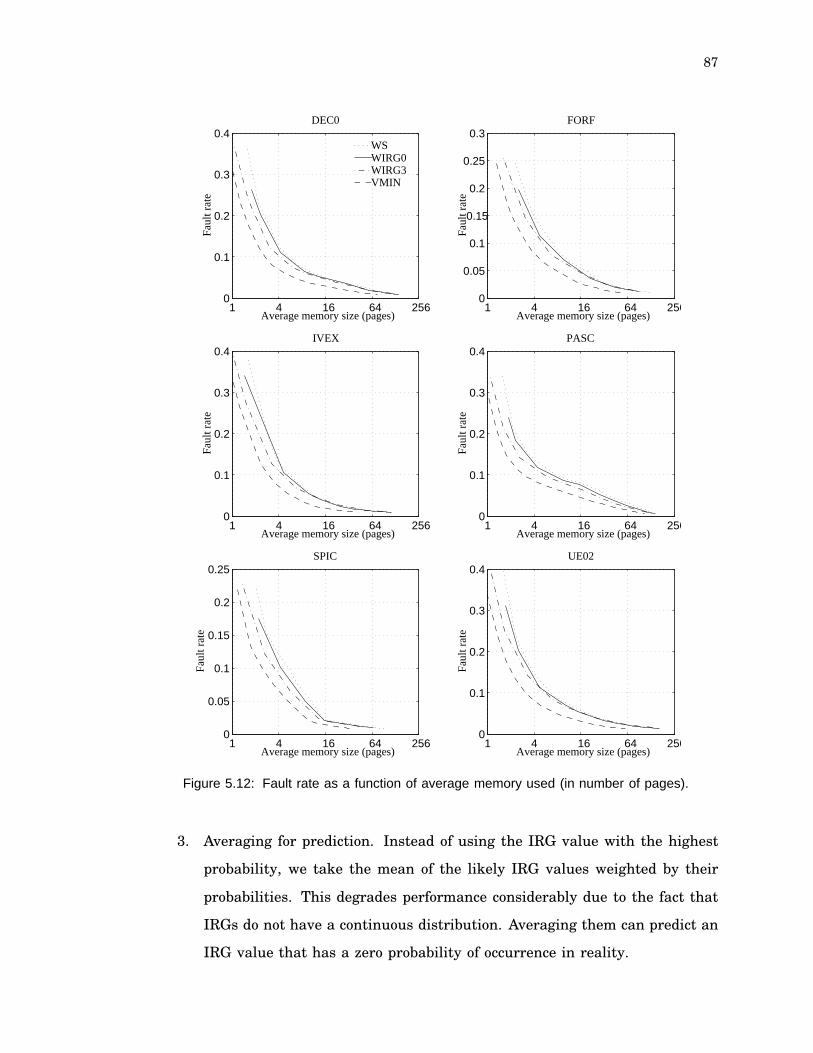
87
1 4 16 64 2560
0.1
0.2
0.3
0.4WSWIRG0WIRG3VMIN
Average memory size (pages)
Faul
t rat
e
DEC0
1 4 16 64 2560
0.05
0.1
0.15
0.2
0.25
0.3
Average memory size (pages)
Faul
t rat
e
FORF
1 4 16 64 2560
0.1
0.2
0.3
0.4
Average memory size (pages)
Faul
t rat
e
IVEX
1 4 16 64 2560
0.1
0.2
0.3
0.4
Average memory size (pages)
Faul
t rat
e
PASC
1 4 16 64 2560
0.05
0.1
0.15
0.2
0.25
Average memory size (pages)
Faul
t rat
e
SPIC
1 4 16 64 2560
0.1
0.2
0.3
0.4
Average memory size (pages)
Faul
t rat
e
UE02
Figure 5.12: Fault rate as a function of average memory used (in number of pages).
3. Averaging for prediction. Instead of using the IRG value with the highest
probability, we take the mean of the likely IRG values weighted by their
probabilities. This degrades performance considerably due to the fact that
IRGs do not have a continuous distribution. Averaging them can predict an
IRG value that has a zero probability of occurrence in reality.

88
�
(miss
pena-
lty)
Normalized Space-Time product ST = AvgMem � (1 + MissRatio � � )
CC1 DEC0 SPIC
WS WIRG0 WIRG3 WS WIRG0 WIRG3 WS WIRG0 WIRG3
Imp. over WS Imp. over WS Imp. over WS
512 323 1.8 7.6 577 3.5 20.2 223 0.5 16.8
1024 667 5.9 7.7 1307 7.5 16.2 529 3.6 16.6
2048 1193 9.7 7.3 2632 6.7 10.6 1156 5.0 14.9
4096 1833 0.7 -3.7 4866 2.3 2.7 2770 1.5 14.1
8192 3397 1.5 -3.1 9234 -3.2 -7.6 6904 0 0
Table 5.6: ST Space-Time Product for the CC1, DEC0 and SPIC simulations.For WIRG0 and WIRG3 we show the % improvement over WS.
�
(misspena-lty)
Normalized R and K errors
WIRG0 WIRG1 WIRG2 WIRG3
R K R K R K R K
512 2.6 12.5 2.7 10.6 2.9 9.8 3.0 9.4
1024 4.8 16.4 5.1 14.6 5.3 13.7 5.4 13.1
2048 6.6 19.8 7.2 17.9 7.4 17.3 7.7 16.7
4096 7.2 24.1 8.0 23.0 8.6 22.4 9.2 21.7
8192 12.6 31.3 13.7 30.5 14.0 29.7 14.7 29.3
Table 5.7: R and K errors for the CC1 simulations.
4. Approximating the prediction by looking only at the last k (some predefined
constant) IRG values in each of the IRG streams. Although storage gets
reduced, prediction becomes difficult as the statistics have to be recomputed
at the occurrence of each new IRG value. A better solution is to maintain
frequency counts in a fixed buffer and use it as a cyclic queue. This slightly
improves performance over WS.
5.7 Conclusions
In this chapter, we presented replacement methods which use the past temporal
characteristics of an address to predict the future behavior. These methods show

89
universal applicability at all levels of the memory hierarchy and we obtain sig-
nificant performance improvements in the miss ratio over other known methods.
We also proposed some approximate strategies which are both practical and better
than other known methods.
The work in this chapter was based on the inherent predictable property of
the IRG streams. In the next chapter we explore other techniques for replacement
which are based on some other properties of program behavior.

90
Chapter 6
More Experiments with Replacement
6.1 From LFU to LRU
In the theoretical study of program reference strings, two models have been used
extensively. These are the Independent Reference Model (IRM) [47], and the Stack
LRU Model (SLRUM) [83]. Most of the other complex models have been derived by
extending these two.
The online optimal replacement algorithm for IRM model is known to be the A0
algorithm [47] which maintains the top k-1 pages with the highest probability of
reference in the memory (k is the memory size). This can be easily approximated
by the Least Frequently Used (LFU) algorithm. In the case of the SLRUM model,
if the strong locality constraint is observed, i.e. Pr(dist=i) ≥ Pr(dist=i+1) for all i,
then LRU has been shown to be the online optimal replacement algorithm [24]. In
practice, LRU and its derivatives have been shown to perform better than LFU, at
all levels of the memory hierarchy [78, 66, 57]. The main drawback of LFU is its
property to hold back items. Even when an item is no longer needed, it is kept in
memory for a much longer period than LRU because it has a high frequency count.
Programs behave in a phase like manner [50, 23], where each phase is marked
by an affinity to a distinct set of memory locations. This can be also observed from
the trace plots in chapter 3. A simple behavioral model to capture this property is
Spirn’s GLM [82] model (refer chapter 2). It is not hard to see that an online optimal
replacement policy in this case is an LFU policy which resets all the reference
counters when the program changes its phase. Since it is a non trivial task to
detect a phase change in a program, we propose a simple technique which uses
exponentially decaying frequency counters, and study its properties (we call it the
EXP algorithm). Specifically,
Ca[t] = �Ca[t� 1] + �t;a

91
where Ca[t] is the reference count of address a at time t, � is the scaling factor (0
<� ≤1), and �t,a is 1 if address a is accessed at time t, else it is 0. In figure 6.1 we
have the detailed pseudo-code for this algorithm. CLOCKis a global timer. MinSet
function returns all items with the minimal counter value. Notice that counters are
decayed only upon a replacement decision.
PROC access(item a, memory M)SetCounter(a,1) ;IF(a not in M)THEN
X = MinSet( SetCounter(m,0): for all m in M);z = Least Recently Used item in X;Replace z by a;
ENDIFRETURN a;
ENDPROC
PROC SetCounter(item p, int i)C[p]= �CLOCK�LAST[p] x C[p] + i;LAST[p] = CLOCK;RETURN C[p];
ENDPROC
Figure 6.1: EXP algorithm for replacement
The space complexity of EXP is mainly due to the floating point counters it has
to maintain (unlike the integer counters which LFU uses). The time overhead is
because to the computation (�CLOCK�LAST[p]) which needs to be done at every replace-
ment decision.
In figure 6.2 we present the miss ratio as a function of � for a 8-way, 32Kb, 4
byte per line cache for the CC1 and KENBUS1 traces. Notice that �=1 is the same
as LFU, and �=0 is LRU. The miss ratio for CC1 for LFU is 33.4%, and for LRU it
is 16.9%. The local minima for this configuration is obtained at �=0.999865, where
the miss ratio is 15.2% (an improvement of 9.8%). To find the effect of associativity,
we find the miss ratios for �=0.9999, for 2-way, 4-way and 16-way caches, with the
number of sets remaining constant. In addition we compute the miss ratios for the

92
LFU, LRU, and OPT algorithms. The comparison is shown in figure 6.2. In addition
we plot the miss ratio for our predictive algorithm BIT0, explained in chapter 5.
0.999 0.9995 10.15
0.2
0.25
0.3
ρ
Mis
s ra
tioρ versus miss ratio for CC1
0.999 0.9995 10.22
0.24
0.26
0.28
0.3
0.32
0.34
ρ versus miss ratio for KENBUS1
ρ
Mis
s ra
tio
2 4 8 160
0.1
0.2
0.3
0.4
0.5LFULRUEXPBIT0OPT
Associativity
Mis
s ra
tio
Miss ratio comparison for CC1
2 4 8 160.1
0.2
0.3
0.4
0.5LFULRUEXPBIT0OPT
Associativity
Mis
s ra
tio
Miss ratio comparison for KENBUS1
Figure 6.2: Performance of the EXP algorithm. � versus miss ratio plots are for a 32Kb 8-wayset associative cache with a 4 byte line size. In the miss ratio comparison EXP uses �=0.9999.
We also validate the EXP algorithm against other traces for different cache
configurations. The results obtained are similar. A value of � very close to 1, results
in a miss ratio better than both LFU and LRU. We also experiment with replacement
in paged memory, object traces, and disk traces. For the page references and disk
traces, LFU is worse than LRU, but the miss ratio as a function of � is monotonic.
Same characteristics are observed for object traces, where sometimes LFU is better
than LRU.
To characterize the behavior of the EXP algorithm for the Independent Reference
Model (IRM), in figure 6.3 we plot the � versus miss ratio plot for a 32Kb 8-way
set associative cache on an IRM trace generated using the probabilities of the CC1

93
0.992 0.994 0.996 0.998 10.5
0.55
0.6
0.65
0.7
ρ
Mis
s ra
tioFigure 6.3: � versus miss ratio plot for the Independent Reference Model
trace. Notice that the miss ratios are much higher than the corresponding original
CC1 trace, and that LFU performs better than LRU.
6.2 Replacement at Level 2 (L2 cache)
When an access misses at a higher level in the memory hierarchy, a reference to the
next level in the hierarchy is made. In the context of cache memory, L2 means the
second level cache which is accessed after a miss in the primary cache. Due to high
locality of reference, primary caches usually have a very low miss ratio. This locality
of reference is lost upon reaching the L2 cache. In this section we investigate the
L2 cache references, and some suitable replacement policies.
We simulate an 8Kb direct mapped cache with 16 byte block size as the primary
L1 cache. In table 6.1 we describe the traces used. These were primarily chosen
because of their long lengths (few hundred million references), such that the number
of references reaching L2 be large enough to make the L2 simulations meaningful.
In order to compare replacement policies at the L2 level, we simulate the OPT
(off-line optimal), LRU, LFU, FIFO, RR (random replacement), and our BIT0 (IRG
based with history maintained forever) and SET0 (IRG based with history being
reset upon replacement) replacement strategies using a 2-way, a 4-way, and a 8-
way L2 cache. The L2 cache size is varied from 32Kb to 2Mb. We use worseness in
the miss ratio with respect to the OPT algorithm, as the performance criteria. In
figures 6.4, 6.5, 6.6, 6.7, and 6.8 we present the OPT miss ratio and the worseness of

94
Trace name Miss ratio at L1
(%)
Number of
references
reaching L2
COMP0: SPEC92 text compressionutility
15.4 24.3M
EQN0: SPEC92 eqntott conversionfrom equation to truth table
7.6 8.9M
ESP0: SPEC92 espress minimizationof boolean functions
7.6 10.5M
KENBUS1: SPEC92 kenbus1simulating 20 users
47.5 2.1M
LI0: SPEC92 lisp interpreter 23.5 34.0M
Table 6.1: Traces used in the L2 simulations
rest of the replacement algorithms for a 4-way set associative cache. Similar results
are obtained for the case of 2-way and 8-way caches.
64Kb 128Kb 256Kb 512Kb 1Mb
Cache size
0
10
20
30
40
50
60
Mis
s ra
tio c
ompa
riso
n %
OPT miss ratio
BIT0 Worse
SET0 Worse
LRU Worse
LFU Worse
FIFO Worse
RR Worse
Figure 6.4: Replacement comparison for 4-way caches for COMP0
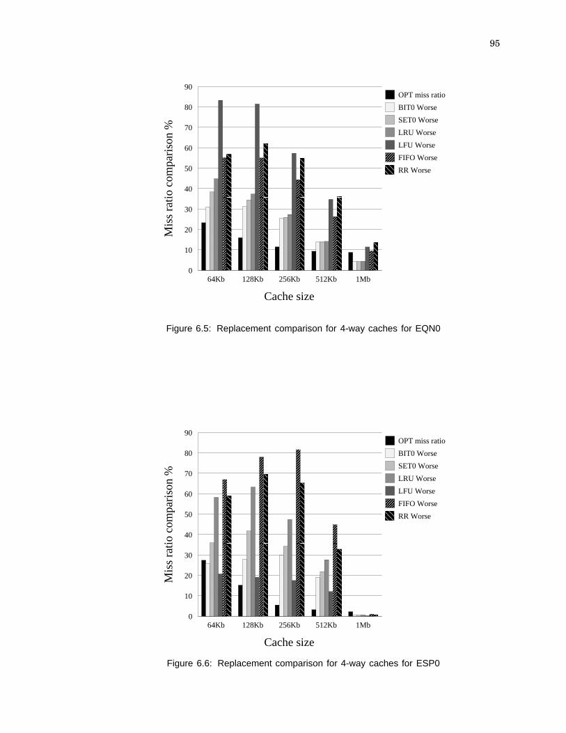
95
64Kb 128Kb 256Kb 512Kb 1Mb
Cache size
0
10
20
30
40
50
60
70
80
90
Mis
s ra
tio c
ompa
riso
n %
OPT miss ratio
BIT0 Worse
SET0 Worse
LRU Worse
LFU Worse
FIFO Worse
RR Worse
Figure 6.5: Replacement comparison for 4-way caches for EQN0
64Kb 128Kb 256Kb 512Kb 1Mb
Cache size
0
10
20
30
40
50
60
70
80
90
Mis
s ra
tio c
ompa
riso
n %
OPT miss ratio
BIT0 Worse
SET0 Worse
LRU Worse
LFU Worse
FIFO Worse
RR Worse
Figure 6.6: Replacement comparison for 4-way caches for ESP0

96
64Kb 128Kb 256Kb 512Kb 1Mb
Cache size
0
10
20
30
40
50
60
Mis
s ra
tio c
ompa
riso
n %
OPT miss ratio
BIT0 Worse
SET0 Worse
LRU Worse
LFU Worse
FIFO Worse
RR Worse
Figure 6.7: Replacement comparison for 4-way caches for KENBUS1
64Kb 128Kb 256Kb 512Kb 1Mb
Cache size
0
10
20
30
40
50
60
70
Mis
s ra
tio c
ompa
riso
n %
OPT miss ratio
BIT0 Worse
SET0 Worse
LRU Worse
LFU Worse
FIFO Worse
RR Worse
Figure 6.8: Replacement comparison for 4-way caches for LI0
From these simulations of the L2 cache, following features about the known
replacement strategies and our methods stand out:

97
1. Miss ratios are very high at the L2 level. For example, for a 2-way 32Kb L2
cache, LRU has miss ratios from 25 to 67%. Even for a large cache like a
8-way 2Mb, the miss ratios are between 2 to 17%.
2. LRU is not unbeatable in comparison to the well known LFU, FIFO, and RR
policies. In fact for the ESP0 trace it is almost as bad as the RR policy.
3. FIFO and RR have similar miss ratios at the L2 level. This has been already
demonstrated for primary cache memories [78].
4. LFU has a very high variation across different benchmarks. In some cases
it performs better than other known techniques and in some cases it is even
worse than RR.
5. Our BIT0 technique, which uses a predictive approach, works the best in
almost all the cases.
6. The SET0 technique, which has a very small overhead, works better than
all the known replacement techniques.
To analyze these properties, consider the L1 cache behavior. It is a direct
mapped cache with 512 sets. The CPU memory reference pattern can be visualized
as an interleaving of 512 disjoint reference streams, where a reference to block r
belongs to stream numbered r mod 512. It is obvious that if we keep the number
of sets the same for the L2 cache, then the references which reach L2 are the same
as that of L1 minus the successive repetitions in each one of the 512 streams. The
successive repetitions all hit at L1. This implies that a policy which works well for
L1, will also work well for L2. To validate this hypothesis, we simulate an L2 cache
with 512 sets and vary the L2 associativity from 2 to 64. In figure 6.9 we present the
worseness of different algorithms with respect to the optimal, for the EQN0 trace.
Similar results are obtained for the rest. We notice that LRU performs better than
other known replacement strategies, and that BIT0 improves upon it.

98
2 4 8 16 32 64
Associativity
0
20
40
60
80
100
120
140
160
Mis
s ra
tio c
ompa
riso
n %
OPT miss ratio
BIT0 Worse
SET0 Worse
LRU Worse
LFU Worse
FIFO Worse
RR Worse
Figure 6.9: Replacement comparison for L2 caches with same number of sets as L1 for EQN0
Interestingly, all replacement algorithms degrade with respect to OPT as the
associativity is increased. This is in contrast to the behavior we saw before where the
cache size is increased by increasing the number of sets. The miss ratio difference
between the OPT algorithm and the other algorithms remains almost constant as
the associativity is increased. This is mainly because of capacity misses which occur
if the working set of blocks mapping to the same set has a size larger than the
associativity. Only when the associativity is made as large as 32, the miss ratios
improve.
6.3 Conclusions
We presented two interesting results for replacement algorithms in this chapter. It
is shown that LFU on a per phase basis can be better than LRU for cache memories.
We believe that with a compiler directed mechanism for signalling phase changes,
LFU can be used for making replacement decisions. Our solution (EXP) needs
floating point counters which can be expensive in today’s VLSI technology.

99
For L2 caches, we showed that LRU need not be the best replacement policy.
LFU proves to be better in some cases. This is mainly because at the L2 level,
references show lesser locality of reference as compared to the L1 level. This was
also proposed in figures 3.13 and 3.14.
We continue with the discussion of cache memories in the next chapter. This
time we look at prefetching using the past history of misses.

100
Chapter 7
A Miss Prediction Based
Architecture for Cache Prefetching
7.1 Introduction
When a program executes, the memory reference behavior is governed by the
principle of locality [84], i.e. the accesses are clustered in space and time. In
addition, programs show correlation across spatially disjoint address spaces, which
we call the inter-cluster locality. This could happen between the code and the data
segment, for example. Another situation where it could happen is in procedure
calls, where the program line making the call and the procedure code itself will
always be correlated in time. Yet another example is the correlation between the
last instruction and the first instruction of a loop. Since miss patterns are a subset
of the reference patterns, it is quite natural to assume that misses would also be
similarly correlated. We aim to exploit this correlation in our prefetch algorithm.
Another important characteristic of the missed references is their fractal nature
[88]. Misses are grouped over time in clusters, each cluster is comprised of smaller
subclusters, each subcluster contains more clusters, and so on. In addition, two
clusters which are made up of misses on almost the same set of memory references,
have similar miss patterns over time. If two such miss clusters are far apart in
time, any simple replacement algorithm, e.g. LRU, will repeat those patterns. On
the other hand, if we “remember” such patterns then we can avoid the misses by
prefetching, if the onset of a repeating miss pattern can be detected quickly enough.
In this chapter, we propose a new prefetch-on-miss technique based on the
history of misses during a program’s execution. We model the sequence of missed
block addresses as a walk on a first order Markov chain. Using this model we predict
the next likely misses and prefetch the blocks predicted to be missed in the future.
Since a complete Markov model is impractical, we only keep an approximation,

101
which is practical. This is done by using extra space at the hierarchy level of the
main memory (which is not expensive) and a bidirectional address bus from the
CPU to the main memory. The extra memory is used to store the Markov model
history of misses. The address bus is utilized in its idle state to notify the CPU as
to which blocks to prefetch next.
We gain significant performance improvement over sequential prefetching via
this technique. For a 4-way cache of 4KB size, and at most one prefetch on amiss, we
obtain miss ratio improvements up to 14% over the sequential technique. In addition
we reduce data bus traffic up to 17% over the sequential method. The corresponding
numbers for a 32KB cache are 14% and 19%, respectively. The improvements in
miss ratio over a non-prefetching scheme are up to 32% and 37%, for cache sizes
of 4KB and 32KB, respectively. The simulations are done over ATUM and SPEC
benchmarks over a wide range of cache configurations. We vary the number of sets,
the associativity, and the block size, with cache sizes ranging from 4KB to 256KB.
In section 7.2 we describe our program model and the prefetching algorithm.
In section 7.3 we give details of our prefetch architecture. In sections 7.4 and 7.5
we evaluate the performance of our system and describe the simulation results.
Finally, in section 7.6 we present the conclusions.
7.2 Program Model and Prefetching
In this section, we first describe the program model and the prefetch technique.
Then we discuss an approximation of this technique suitable for cache prefetching.
7.2.1 Model of Prefetching
Let a program memory access behavior be represented as a reference string Rt =
r1r2...rt. Here each ri is a memory block address to which the ith reference is made.
Let F(Rt, m) = ri1ri2ri3... denote the sequence of block addresses where misses
happen upon executing Rt. Assume the string F(Rt, m) is generated by a first-order
Markov chain, where each rik represents a state. The best estimate of such a Markov
chain is done by a probabilistic finite state machine P(F) defined as follows :

102
1. P(F) has N(F) number of states where N(F) is the number of unique symbols
in F(Rt, m). Each state is labelled by the corresponding block address.
2. In P(F), a directed edge connects state u to v iff substring “uv” (u followed
by v) occurs in F(Rt, m). The probability associated with such an arc is the
ratio of occurrences of substring “uv” in F(Rt, m) to that of u in F(Rt, m).
We illustrate this model by an example. Refer to figure 7.1. P, Q, R, and S are
unique block numbers. In the past, a miss on block P is followed by a miss on block
Q, K1 number of times. A miss on P is followed by a miss on R, K2 times, and by
a miss on S, K3 times. The probability of a miss occurring on block X (X = Q, R, or
S), given that a miss occurs at block P, is given by Pr(P,X).
Pr(P,Q) = K1 / ( K1 + K2 + K3 )Pr(P,R) = K2 / ( K1 + K2 + K3 )Pr(P,S) = K3 / ( K1 + K2 + K3 )
P
Q
R
S
K1
K2
K3
Figure 7.1: Probability estimates for misses on block P followed by misses of blocks Q, R, and S
Let a miss occur at block reference u. Let state u have outgoing edges to states
v1, v2... in P(F). The arcs with the highest probability of transition amongst (u, v1),
(u, v2)... are found and the corresponding blocks (vi’s), up to a maximum of k (a
prespecified parameter), are prefetched.
If the string of misses is known to be generated by a first-order Markov chain,
the above described method is a provably optimal online prefetcher for a fixed k
[21]. But this method cannot be directly applied for cache prefetching due to its
large computations. Hence we will approximate it as per the requirements of our
caching environment.

103
7.2.2 A simple k predictor
Consider the following execution of a pseudo assembly program :
loop: ld [X], %r0 /* Load r0 with word at location Xld [Y], %r1 /* Load r1 with word at location Y::: /* Instructions with no reference to X or Ybne loop /* Loop back
Assume memory words X and Y are in different main memory blocks and the blocks
containing the above instructions are already in the cache. A miss happens on
memory word X. At the next instruction, a miss occurs on memory word Y. If we
remember this sequence of misses, then the next time a miss occurs at X, we not
only fetch the block containing X, but also prefetch the block containing Y. This
could happen, for example, if the loop in the above example is large enough to flush
X and Y out of the cache by the time it returns to the line labelled loop .
There are three main reasons why we expect this method to show significant
performance improvement :
1. First, since successive memory accesses tend to be correlated, the misses will
also be. This has been demonstrated empirically by Haikala [38]. Further,
Puzak [63] has shown that the sequence of misses captures the temporal
features of the original reference string. Therefore, by maintaining a model
of the misses we can “remember” most of the behavioral characteristics of
the original reference stream.
2. Second, miss patterns repeating after long periods of time are “forgotten”
by most of the cache management algorithms. For example, if a reference
substring repeats after a reasonably long gap, then LRU will have identical
miss patterns at both times. This can be avoided, assuming that we can
store the miss correlations over long periods of time.
3. Finally, between two consecutive misses there will usually be a sequence of
hits (on an average (miss ratio)�1 hits). Thus, for low miss ratios we expect
a large number of prefetches to complete successfully, i.e. a miss does not
happen before the prefetch is over. This is in contrast to a reference stream
model [21], where the very next reference is predicted and prefetched.

104
We limit our predictor to prefetch k blocks on a miss, k being a constant. Upon
a miss on block b, we need to know the k most likely misses which will happen
next. This is done by “remembering” the last k misses which had followed the miss
on block b in the past. The k entries are maintained as a simple FIFO buffer for
ease of implementation. We illustrate this process by an example. Consider the
sequence of missed blocks as “0 2 1 2 1 0 1 4 2 3 1 4”. For k equal to 2, the history
will look as follows:
Current State Probable Next
State
0 1 2
1 4 0
2 3 1
3 1 -
4 2 -
In this way, we approximate the optimal Markov model described in section
7.2.1 in the following ways:
1. The k highest probabilities of transition out of a state are approximated by
a FIFO ranking. Keeping the count of each transition will involve keeping
all the outgoing edges, which is expensive, and therefore not done.
2. An access to a prefetched block (a miss in the original non-prefetch scheme)
does not lead to a Markov model transition. This assumption is needed since
a transition involves prefetching and book keeping, which is too expensive
to do upon each hit.
7.3 Architecture of the Prefetcher
In this section, we describe the architecture of our prefetching hardware. It is
presented assuming a very simple cache-main memory organization. However,
it should be noted that we are doing this only for the sake of completeness, and
the main emphasis is on the model of prefetching and its results. The actual

105
implementation will vary depending on the type of memory, processor and other
hardware parameters. We also describe an alternate technique for prefetching
which can be built by merely changing the CPU control logic.
We specify a cache by three parameters, B is the size of the block - the smallest
unit of data transfer between the cache and the main memory, S is the number of
sets in the cache, and A is the associativity of each set. We use the triple (S, A, B)
to represent a cache configuration. The caches use the Least Recently Used (LRU)
technique for replacement in each set. Each prefetched block is placed in the least
recently used slots of the set.
7.3.1 Prefetch Architecture
We maintain a separate prefetch engine to keep the Markov model approximation,
and to initiate prefetches. This prefetch engine is at the same level in the memory
hierarchy as the main memory. It has the capacity to read-write on the address
bus, much like a DMA device. In addition it can reverse the direction of the address
bus, and send data to the CPU. For storing the history of misses, it has a memory
table called the signal buffer, made up of M rows with k entries in each row. M
is the total number of blocks in main memory. Each row b of the signal buffer is
a FIFO buffer, which stores the addresses of the blocks (up to a maximum of k),
which were missed right after a miss on block b in the past. A single register L is
used to store the latest miss address.
The CPU needs a bank of k registers to store the prefetch addresses sent by the
prefetch engine. This is not a significant overhead since k is 1 or 2 (due to reasons
of practicality we can not prefetch larger number of blocks in a cache environment).
Figure 7.2 has the block diagram of our architecture.
We note that when a block is accessed for the first time, it causes a cold miss.
This will not trigger any history based prefetches. If the number of cold misses is
very high, it can degrade performance considerably. To alleviate this problem, our
prefetch engine incorporates sequential prefetching upon a cold miss, i.e. when the
history information of a missed block b is null, then it prefetches block b+1, for k
equal to 1. Initially, row b of the signal buffer contains values b+1, b+2, ... b+k.

106
CPU
Blk 0Blk 1
Main Memory
.
.
.
Data Bus
Address Bus
PrefetchAddressBus
PrefetchRegisters
Set S-1
Cache Memory
Slot 0 Slot 1 Slot A-1 Set 0 Set 1 . . .
.
.
.
.
.
.
Prefetch Engine
A 0 A 1 A k-1
Signal Buffer
L . . ...
0
M-1
Blk M-1
Figure 7.2: Block diagram of the prefetch architecture
When a miss occurs on block b, the CPU places the value b on the address bus.
This value is latched on by main memory which then starts transferring data from
the main memory block b to the cache. The prefetch engine inserts b in the signal
buffer row pointed to by L. L is then updated to point to row b of the signal buffer.
Next the prefetch engine reverses the address bus (it is idle at this point), and puts
out the k entries from the row pointed to by L on the address bus. This is done
in k clock cycles, after which, the address bus direction is restored back. The CPU
stores the k prefetch addresses received from the prefetch engine in its prefetch
registers. We assume that main memory to CPU data transfer (fetch on miss) takes
more than k clock cycles (k is typically 1 or 2).
After the missed block is brought in the cache, the CPU has k addresses to
prefetch. It matches these addresses against the cache tags and initiates prefetches
for the blocks that are not in the cache. If a prefetch is successful, i.e. a miss does
not occur before it is completed, then that prefetched block is placed in the least
recently used slot of the cache.
The issue of another miss occurring before a prefetch is over, is an orthogonal
problem. What we have provided is an “oracle” to the CPU which does not alter
the timing sequence. All it does is give a “smart” choice for prefetching. This is

107
CLOCK
REV
MISS
(2) Prefetch engine reverses address bus
(3) k = 2 Prefetch addresses sent fromthe prefetch engine to the CPU
(4) Prefetch enginerestores address bus
(1) Missed block address latched by main memorySignal buffer update carried out
AddressBus
Figure 7.3: Timing diagram for the prefetch architecture
done with a small overhead at the main memory level. For a block size of 16 words
per block, and k equal to 1, the size of the signal buffer will be 1/16th of the main
memory (a 6.25% increase).
Now we address the issue of the bidirectional address bus in more details. DMA
is an instance where an address bus is used both by the CPU and another device.
In the case of DMA, the address bus is used for main memory read or write. We
however need to use it to send an address value to the CPU. This can be easily
achieved by an extra control line which the prefetch engine has the ability to turn
on or off. During a miss processing, when the address bus becomes idle, the REV
(reverse) control line is turned on by the prefetch engine, disabling any input to the
main memory. Simultaneously it disconnects the MAR (memory address register) of
the CPU and redirects the traffic of the address bus into the CPU prefetch registers.
REV is turned off by the prefetch engine after the prefetch address transfer is over.
A timing diagram is given in figure 7.3.
Another issue is the design of the prefetch engine. It needs the ability to snoop
on the address bus and find out when a miss happens. This can be done obviously.

108
The prefetch engine also needs to update its miss history efficiently, which can be
done by maintaining each row in the signal buffer as a cyclic FIFO. The cyclic part
is needed to read off the k entries. We can use the address decoding logic of the
main memory itself to set the L pointer in the prefetch engine. Alternately, the
entire prefetch engine can be built as part of the main memory design itself. With
each main memory block we attach additional k memory words to store the history.
But this scheme will need multiple ports to the main memory, since the fetch and
the history prediction needs to be carried out in parallel.
Finally, we present the prefetch-to-access delay characteristics of our technique.
We define prefetch-to-access delay as the number of memory references between
the time a block is prefetched and the time when it is actually accessed. Here we
only count the “useful” prefetches, i.e. a prefetch which avoids a miss. This delay
quantifies the time available for carrying out the actual prefetch. More the prefetch-
to-access delay, greater is the CPU flexibility in bringing in a block. This is suitable
for pipelined prefetching where a prefetch is pipelined (delayed) when a miss occurs
before the prefetch is complete. Obviously, the prefetch-to-access delay has no effect
on a prefetcher which aborts prefetching if a miss happens.
Figure 7.4 has the cumulative distribution of the prefetch-to-access delay value
for the KENS trace, simulating a 4KB, 4-way set associative cache, with block size
16 words. SEQL denotes the distribution for the sequential prefetching, and HIST
is our technique with k equal to 1. In general, (as observed from other experiments
too), our method has a larger prefetch-to-access delay than the sequential technique.
7.3.2 A simpler in-cache Architecture
A simpler architecture in comparison to the one described above is one where
the prefetch engine is maintained as part of the CPU-cache unit itself. In this
architecture no modifications are needed to the CPU or the address bus, only the
CPU control logic needs to be changed. Obviously, we can not maintain the entire
signal buffer in cache, e.g. for a 24 bit address machine, with 16 words per block,
and k equal to 1, we need a 4MB signal buffer – obviously infeasible. Hence we
keep the Markov model of only l number of states, where l is typically 1K or less.

109
0 5 10 15 20 25 30 350
0.1
0.2
0.3
0.4
0.5
0.6
0.7
0.8
0.9
1
Prefetch-to-access delay
Cum
ulat
ive
Dis
trib
utio
n
___ SEQL- - - HIST
Figure 7.4: Prefetch–to–access delay for KENS trace, for a 4KB cache
This restriction will add one extra field to the signal buffer since we will need to
store the Markov model transitions as a pair of states.
Assume a miss happens on block a, followed by a miss on block b. First we
search for an entry corresponding to a in the signal buffer. If it exists then we add
b to its FIFO queue. If it does not then we create a row for a and add b to it. In
case the signal buffer is full, we use the FIFO policy to purge an entry. Next, we
look for an entry for block b. If the entry exists, then we prefetch the k addresses
given in that entry.
The overheads, besides the size of the signal buffer, are the adding of a new
row to the signal buffer when all its rows are occupied, and the search for a block
address upon a miss. The addition of a new entry is simply done in a FIFO manner
by maintaining the rows as a cyclic queue. This obviously implies that we “forget”
some history. The search is carried out associatively, which can be expensive for
large number of entries. However, it occurs only upon a miss, providing us with a
large time interval for carrying it out. Additionally, this expense can be reduced by
partitioning the signal buffer into sets (like the cache) and doing the search only in
a set, or by using a fast hashing technique.
The overheads of such a technique can be reduced by increasing the block size.
This will decrease the total number of unique block references, and hence the signal
buffer search will be reduced.

110
Tag Data
CPU
Signal Buffer
L
S A1 A2 Ak
Main memory blocks
Address bus Cacheblocks
Figure 7.5: In-cache architecture
7.4 Simulation Description and Results
We do performance evaluation of our architecture using ATUM and SPEC bench-
mark traces, and in this section we present the results. These traces are described
in table 3.1.
We use two figures of merit to evaluate our technique. One is the miss ratio
improvement over a non-prefetching scheme, and the other is the increase in
data bus traffic, due to prefetching. Since our comparison basis is the sequential
technique, we also present results for the same. In the following discussion we refer
to the sequential method as “SEQL”, and our technique as “HIST”. Throughout, we
use the term memory word to imply 4 bytes, and unless otherwise noted, k - the
maximum number of prefetches upon a miss, is 1 block. We also assume that no
prefetch is aborted, which means that in reality, the performance figures will be
lower than those presented here.

111
For algorithm A, the two figures of merit are defined as:
Miss ratio improvement :
Amiss imp =miss ratio(NONPREF) � miss ratio(A)
miss ratio(NONPREF)
Increase in data traffic :
A traffic inc =#miss(A) + #prefetch(A) � #miss(NONPREF)
#miss(NONPREF)
Where NONPREF refers to the non-prefetching, fetch-on-demand strategy. #miss is
the total number of misses, and #prefetch is the total number of blocks prefetched.
To limit cache simulation time, only the first 5 million references from each
benchmark, or the trace length, whichever smaller is used. Results using the
full reference streams are similar. Moreover, the relative merit of our technique
increases for longer traces, since it “learns” more about the history of misses.
Since the total number of benchmarks is large, we only present a summary
for them in this section (in section 7.5 we have plots for all traces). After that
we present results describing the effect of changing various cache and prefetch
parameters using DEC0 and LISP as the “representative” benchmarks. Results are
similar for other benchmarks.
7.4.1 Summary of results for a 4-way 4KB cache
In figure 7.6 we plot the miss ratio improvements with respect to a non-prefetching
cache, for both the SEQL and HIST techniques, for all traces. The cache is a 4KB,
4-way set associative cache with a block size of 16 words (represented by ( 16, 4, 16)
– using the notation in section 7.3). LRU policy is used in each set for replacement.
Figure 7.7 shows the increase in data bus traffic with respect to a non-prefetching
scheme for the same set of simulations.
Using our technique, all the benchmarks show a 25 to 32% improvement in the
miss ratio over the non-prefetching scheme. In addition, bus traffic is substantially
reduced in comparison to the sequential method.

112
CC
1
DE
C0
FOR
A
LIS
P
MA
CR
MU
L8
PASC
SPIC
CO
MP0
EQ
N0
KE
NS
LI0
Benchmark
0
5
10
15
20
25
30
35
Impr
ovem
ent i
n m
iss
ratio
(%
)
HIST
SEQL
Figure 7.6: Miss ratio improvement in a4KB, 4-way set associative cache
CC
1
DE
C0
FOR
A
LIS
P
MA
CR
MU
L8
PASC
SPIC
CO
MP0
EQ
N0
KE
NS
LI0
Benchmark
0
10
20
30
40
50
60
Incr
ease
in d
ata
bus
traf
fic
(%)
HIST
SEQL
Figure 7.7: Increase in data traffic in a4KB, 4-way set associative cache
7.4.2 Effect of cache size on performance
We study the effect of cache size on our prefetching scheme, by varying the number
of sets from 16 to 4K. Figure 7.8 shows the plots where the block size is 16 words,
and the cache is 4-way set associative, i.e. ( *, 4, 16) caches. We also simulate a
direct mapped cache with 16 words per block. Figure 7.9 has the corresponding
plots. Results are similar for different block sizes.
SEQL miss imp
HIST miss imp HIST traffic inc
SEQL traffic inc
4K 16K 64K 256K15
20
25
30
35
40
45
Cache Size (bytes)
Perc
ent c
hang
e
DEC0
4K 16K 64K 256K10
20
30
40
50
60
Cache Size (bytes)
Perc
ent c
hang
e
LISP
Figure 7.8: Miss ratio improvement and bus traffic increase versus cache size for a 4-way cache

113
SEQL miss imp
HIST miss imp HIST traffic inc
SEQL traffic inc
4K 8K 16K 32K 64K15
20
25
30
35
40
45
50
Cache Size (bytes)
Perc
ent c
hang
e
DEC0
4K 8K 16K 32K 64K0
20
40
60
80
Cache Size (bytes)
Perc
ent c
hang
e
LISP
Figure 7.9: Miss ratio improvement and bus traffic increase versus size of a direct mapped cache
Although the overall miss ratio goes down with an increase in the number of
sets (in figure 7.8, for DEC0 trace, the non-prefetching miss ratio reduces from 19%
to 2%), the miss ratio improvements and the traffic increase stays constant. This
implies that the misses which get eliminated due to the increase in the number of
sets, do not drastically change the regularities in the original miss patterns. For
example, the original miss string “... abc ... abc ...”, on increasing the number of
sets, will change to “... ac ... ac ...”. This is also obvious from the way set mapping
is done. In the above example, if a miss on a triggers a prefetch of block b in the
original case, then for the larger number of sets, a miss on a will prefetch block c,
preserving the miss ratio improvements.
On a side note, this explanation can not be applied for the case when the cache
size is increased via an increase in the set size. This is due to the fact that regularity
can not be guaranteed for the eliminated misses when they are governed by the LRU
stack behavior of other blocks in the set.
An important issue for the direct mapped cache is the case where a prefetched
block maps onto the same block which is just missed. If we assume that the CPU
accesses the missed block prior to the prefetched block coming in, then we do not
need to change our architecture. Otherwise, we will have to either delay the prefetch
or abort it. In our experiments we find that less than 5% of the prefetches map to the

114
Trace Cache
size (KB)
Non
prefetch-
ing miss
ratio (%)
SEQUENTIAL HISTORY
Miss ratio
(%)
Useful
prefetches
(%)
Miss ratio
(%)
Useful
prefetches
(%)
DEC0 4 19.3 15.0 37 13.9 51
16 12.3 8.95 48 8.53 61
64 5.3 4.00 51 3.81 62
256 2.1 1.47 53 1.46 56
LISP 4 19.3 16.3 30 14.0 60
16 3.22 2.79 33 2.41 64
64 0.93 0.73 51 0.68 66
256 0.61 0.42 65 0.42 65
Table 7.1: Ratio of useful prefetches for a 4-way set associative cache
same block as the one just missed. For such low values, neglecting these prefetches
will not degrade the HIST performance significantly.
For a direct mapped cache, we also compare our method against Jouppi’s stream
buffer [43] of length 1. For the DEC0 trace, his method yields a miss ratio
improvement of 15% for a 32KB direct mapped cache with 16 word lines. On the
other hand, for the same configuration, SEQL yields a 21%, and our technique yields
a 24% miss ratio improvement. For other traces too, his technique with stream
length 1 does not show any significant improvement over the sequential technique.
An important feature of any prefetch algorithm is the number of useful
prefetches, i.e. a prefetch that results in a miss getting avoided. Table 7.1 lists the
ratio of useful prefetches to the total prefetches for the simulations in figure 7.8.
The percentage of useful prefetches for our technique is much larger than that of
the sequential technique.
7.4.3 Effect of degree of associativity on performance
Keeping the block size and the number of sets fixed, we vary the number of blocks in
a set and evaluate its impact on our technique. Figure 7.10 presents the miss ratio
improvement and the data traffic increase for both the SEQL and HIST methods,

115
where the block size is 16 words per block and the number of sets is 16, i.e. ( 16, *,
16) caches. Results with block size of 4 words, and 64 and 256 sets, are similar.
SEQL miss imp
HIST miss imp HIST traffic inc
SEQL traffic inc
1 2 4 8 16 3215
20
25
30
35
40
45
50
Degree of associativity
Perc
ent c
hang
e
DEC0
1 2 4 8 16 320
20
40
60
80
Degree of associativityPe
rcen
t cha
nge
LISP
Figure 7.10: Miss ratio improvement and bus traffic increase versus associativity
As the cache size is increased by increasing the number of blocks per set, the
number of hot misses goes down. Hot misses are those which are caused due to the
cache being too small to accommodate the entire “working set”. These hot misses
are the ones which primarily assist our algorithm. As they reduce in number, cold-
misses start dominating, and our algorithm degenerates to the sequential technique
for very large associativity.
7.4.4 Effect of block size on performance
We vary the block size, keeping the number of sets and the set size (in terms of
memory blocks) constant. Figure 7.11 presents plots for miss ratio improvement
and data bus traffic increase, for a 4-way cache with 16 sets, i.e. ( 16, 4, *) caches.
Results for direct mapped, as well as 64 and 256 sets per cache, are similar.
As the block size is increased, for both the techniques, the miss ratio improve-
ment decreases. This is expected since sequentiality gets reduced due to merger of
consecutive blocks to create larger blocks. This reduction in sequentiality is also
evident from the fact that the performance gap between our technique and the se-
quential technique (see figure 7.11) increases with the block size. On the other

116
SEQL miss imp
HIST miss imp HIST traffic inc
SEQL traffic inc
4 8 16 32 6415
20
25
30
35
40
45
50
Block Size (words)
Perc
ent c
hang
e
DEC0
4 8 16 32 640
10
20
30
40
50
60
Block Size (words)
Perc
ent c
hang
e
LISP
Figure 7.11: Miss ratio improvement and bus traffic increase versus block size
hand, the correlation between spatially far apart addresses (inter-cluster locality)
in a large address space (32 bit, for example), is independent of small block size (4
to 64 words per block), and therefore the predictive part of our architecture is not
affected by the block size.
7.4.5 Prefetch k = 2, 4, 8 blocks on a miss
Although k = 8 is impractical for certain cache architectures, we simulate our archi-
tecture for that value also. This is done so as to study the miss ratio improvement as
a function of k. We compare our technique against the general sequential method,
where upon a miss on block a, blocks a+1, a+2... a+k are prefetched. Figure 7.12
has the miss ratio as a function of k for both sequential and our technique. In the
figure, k equal to 0 denotes the non-prefetch miss ratio. The plots are for a 16KB,
4-way cache with a block size of 16 words. Figure 7.13 has the increase in data bus
traffic for the plots depicted in figure 7.12.
Interestingly, the sequential technique degrades for higher values of k. Al-
though the number of prefetches go up, the miss ratio more or less remains con-
stant. This is mainly due to unneeded blocks (blocks which will not be accessed at
all) displacing blocks from the “working set”. On the other hand, for higher values
of k, our technique works well, wherein the miss ratio is brought down by more
than 50% at the cost of doubling the data bus traffic.

117
HIST SEQL
0 2 4 6 80.04
0.06
0.08
0.1
0.12
0.14
Max prefetch on a miss (k)
Mis
s ra
tio
DEC0
0 2 4 6 80.015
0.02
0.025
0.03
0.035
Max prefetch on a miss (k)
Mis
s ra
tio
LISP
Figure 7.12: Miss ratio as a function of k
HIST SEQL
0 2 4 6 80
50
100
150
200
250
300
350
Max prefetch on a miss (k)
Incr
ease
in d
ata
bus
traf
fic
(%)
DEC0
0 2 4 6 80
100
200
300
400
500
Max prefetch on a miss (k)
Incr
ease
in d
ata
bus
traf
fic
(%)
LISP
Figure 7.13: Increase in data bus traffic as a function of k
7.4.6 Instruction Prefetching vs Data Prefetching
Our architecture, as presented, can not distinguish between instruction references
and data (operand) references. Minor modifications to the prefetch engine, and a
control line from the CPU can add this facility. To find out the domain (instruction
stream or data stream) which chiefly benefits from our technique, we simulate
separate instruction (I) and data (D) caches. A miss in the data cache triggers
a prefetch only in the data cache and the same holds for the instruction cache.
Thus we maintain two parallel histories at the prefetch engine level. In figure 7.14

118
we present the miss ratio improvement and traffic increase for the DEC0 trace, for
the two separate streams. Both the I and D caches are 4-way set associative with
16 words per block.
SEQL miss imp
HIST miss imp HIST traffic inc
SEQL traffic inc
4K 16K 64K 256K0
10
20
30
40
50
Cache Size (bytes)
Perc
ent c
hang
e
DEC0 Instruction Prefetching
4K 16K 64K 256K0
10
20
30
40
50
60
70
Cache Size (bytes)
Perc
ent c
hang
e
DEC0 Data Prefetching
Figure 7.14: Miss ratio improvement and bus traffic increaseversus cache size for I and D caches
From these plots, it is obvious that instruction streams are, in general, highly
sequential. For the I cache, both techniques – sequential and ours, perform very
well. Although, for smaller caches our technique works better – it has a lower bus
traffic increase.
By using separate data and instruction histories, the overall miss ratio improve-
ment is lower than a common history cache (see figure 7.8). This is due to the fact
that we do not use the correlation between the code and the data to prefetch.
7.4.7 In-Cache prefetch engine
Finally, we discuss the simulation results where the signal buffer is part of the
cache, as described in section 7.3.2. We present results for two signal buffer sizes.
One has 256 rows and the other has 1K rows. In both the cases k is equal to
1. Assuming each block address takes one memory word, a 256 row signal buffer
will need 2KB space. Similarly for 1K rows we need a 8KB signal buffer. In figure
7.15 we present the miss ratio improvement and data bus traffic increase for the two

119
signal buffer configurations, with 4-way, 16 words per block caches. For comparison,
we also show the values for the original architecture which has no limitations on
the size of the signal buffer.
HIST miss imp HIST traffic inc
SigB=1K miss imp SigB=1K traffic inc
SigB=256 miss imp SigB=256 traffic inc
SEQL miss imp SEQL traffic inc
4K 16K 64K 256K15
20
25
30
35
40
45
Cache Size (bytes)
Perc
ent c
hang
e
DEC0
4K 16K 64K 256K10
20
30
40
50
60
Cache Size (bytes)
Perc
ent c
hang
e
LISP
Figure 7.15: Miss ratio improvement and bus traffic increase for the in-cache architectures
For caches of all sizes, the in-cache technique yields significant improvements
over the sequential method. However, this gain is annulled for small caches due
to the extra space taken by the signal buffer. On the other hand, increasing the
block size decreases the signal buffer size limitations, since the number of unique
blocks goes down.
7.5 Performance of Remaining Benchmarks
In figures 7.16 and 7.17 we present the miss ratio improvement and the increase in
data bus traffic values for the sequential method (SEQL) and our technique (HIST)
for all the benchmarks. The cache is a 4-way set associative cache with 16 words
per block. The cache size is varied by increasing the number of sets. Maximum
number of prefetches at each miss (k) is 1 block.

120
SEQL miss imp
HIST miss imp HIST traffic inc
SEQL traffic inc
4K 8K 16K 32K 64K 128K10
15
20
25
30
35
40
Cache Size (bytes)
Perc
ent c
hang
e
COMP0
4K 8K 16K 32K 64K 128K20
25
30
35
40
Cache Size (bytes)
Perc
ent c
hang
e
EQN0
4K 8K 16K 32K 64K 128K15
20
25
30
35
Cache Size (bytes)
Perc
ent c
hang
e
KENS
4K 8K 16K 32K 64K 128K15
20
25
30
35
Cache Size (bytes)
Perc
ent c
hang
e
LI0
Figure 7.16: Miss ratio improvement and bus trafficincrease versus cache size for the SPEC92 traces
7.6 Conclusions
We have defined a notion of inter-cluster locality to explain the predictable nature
of misses in a non-prefetching cache. We have proposed a Markov model based tech-
nique for capturing this behaviour, and have used that model to prefetch in a cache
memory environment. A simple prefetch-on-miss architecture, which does not add
to the complexity of the CPU, is proposed to implement this technique. It involves
a minor increase in main memory size (less than 6.25%) and a bidirectional ad-
dress bus, both of which are extensions of a practical nature. We have analyzed the
performance of our technique using ATUM and SPEC benchmark traces, obtaining
significant miss ratio improvements over conventional schemes. For a 4-way set
associative 32KB cache, with at most one prefetch on a miss, we obtain consistent

121
SEQL miss imp
HIST miss imp HIST traffic inc
SEQL traffic inc
4K 8K 16K 15 64K10
15
20
25
30
35
Cache Size (bytes)
Perc
ent c
hang
e
CC1
4K 8K 16K 32K 64K20
25
30
35
40
45
Cache Size (bytes)
Perc
ent c
hang
e
FORA
4K 8K 16K 32K 64K15
20
25
30
35
40
45
50
Cache Size (bytes)
Perc
ent c
hang
e
MACR
4K 8K 16K 32K 64K15
20
25
30
35
40
Cache Size (bytes)
Perc
ent c
hang
e
MUL8
4K 8K 16K 32K 64K10
15
20
25
30
35
40
Cache Size (bytes)
Perc
ent c
hang
e
PASC
4K 8K 16K 32K 64K10
15
20
25
30
35
40
45
Cache Size (bytes)
Perc
ent c
hang
e
SPIC
Figure 7.17: Miss ratio improvement and bus trafficincrease versus cache size for the ATUM traces
miss ratio improvements over a non-prefetching scheme in the range of 23 to 37%.
The increase in bus traffic, in this case, is in the range of 11 to 39%. In compari-
son to the sequential method, the miss ratio improvements are up to 14% and the

122
reduction in bus traffic is up to 17%. Similar improvements over the sequential
technique are obtained for larger and direct mapped caches. For the case where
up to 8 prefetches are allowed on a miss, the miss ratio improves up to 30% over
the sequential method.
We have provided a Markov model based “oracle” to the CPU to identify which
blocks to prefetch. In conjunction with the recent results of Song and Cho for
virtual memory [81], and Griffioen and Appleton for file systems [35], this technique
implies that history based systems can provide substantial improvements in memory
management algorithms at all levels of the hierarchy.
In the next chapter, we shift our focus on to the next levels of the memory
hierarchy, i.e. the page level in a virtual memory setting, disk blocks and database
buffer management. We propose new measures for the space-time product, and
propose online optimal algorithms for page management.

123
Chapter 8
Space-Time Trade-off in Virtual Memory
8.1 Introduction
In a multiprogrammed uniprocessor paged environment, the two most important
criteria on which the overall system performance depends are, memory usage, and
the fault rate of each process. Memory is a shared resource among multiple pro-
cesses which makes it a critical parameter – unlike the fixed space uniprogrammed
scenario where reducing the fault rate is the only concern. A number of pages re-
side on a secondary store, like a disk, and a subset of them are present in main
memory. A simplified view is shown in figure 8.1. Here processes P and Q use
pages p1, p2, p3 and q1, q2, respectively. Out of which, pages p2, q1, and q2 are
currently in main memory.
P Q
p1 p
2p3
q1
q2
Processes
Main memory(Limited space)
Disk (Virtual space)
p2
q1
q2
Figure 8.1: A simplified view of a paged memory
We model the time-instances at which references to a page p are made, using
the Inter-Reference-Gap (IRG) sequence for a page. If page p is accessed at times
ti, i=1, 2, 3, ... (from any process), then the sequence of IRGs is ti+1�ti, i=1, 2,
3, .... Here time ti could be real (absolute time) or virtual (at each clock tick one
page is referenced). Using this IRG model for each page, we study the space and

124
time trade-off. Specifically, we assume a demand fetched scenario, where a page is
brought into memory only on a fault, and can be removed to the disk at any time.
Space is computed as the total duration of stay of a page in main memory, and time
is computed as the number of faults on that page.
We show the following results:
1. For a fixed fault rate on a page, the lower bound on space is achievable by
an online randomized policy.
2. When the overall space-time cost for a page is defined as a linear combination
of space and time, the online optimal policy is deterministic.
In related work, Denning [26] defines the well known Working Set (WS) notion
for memory management. Under this policy, pages accessed in the last � memory
accesses are kept in memory. By varying � , the trade-off in average space versus
fault rate can be found under this model. Although practical, this policy does not
propose any notion of optimality. On the other hand, Prieve and Fabry [61] propose
an optimal strategy VMIN, which achieves the minimal average space for a fixed
fault rate. Their technique needs to know the next � memory accesses a priori, and
hence is not online.
Other related work on space-time trade-off in virtual memory has focussed on
reducing maximum working set size [74], generalizing the WS notion to segments
[25], and analyzing the working set characteristics[11, 58, 37, 41]. A comprehensive
review of these papers has appeared in Denning’s paper [23].
8.2 Definitions
Let page p be referenced, by any process, at times t1, t2, t3, ..., etc. To simplify, we
consider time to be virtual, i.e. at each unit of time, some page is referenced.
Define: The Inter-Reference-Gap (IRG) is defined as the duration of time be-
tween successive references to page p. The sequence of IRGs for page p are t2�t1,t3�t2, t4�t3, ..., and so on.
Example:

125
12 72 80 136 150 172
IRG(p) = ... 60, 8, 56, 14, 22, ...
Reference times for page p:
Define: Independent-Gap-Model (IGM). We model the IRG values for a page p,
as a sequence of i.i.d. random variables. The range of the IRG values is I+, the set
of positive integers. The probability of an IRG value being i is fixed at gi, and is
independent of the history of IRGs. Obviously,Pi2I+
gi = 1.
Space sp : We measure space via the duration of stay of page p in memory, i.e.:
sp =Lt
T !1
KTPi=1
(ri � bi)
T
where sp is the normalized duration of stay of page p in memory. T is the total time
since the first reference to page p, KT is the number of times page p is faulted on
up to time T, bi is the time instant of the ith fault on p, and ri is the time when
page p is removed from memory after its ith fault. If the page hasn’t been removed
after the KTth fault, then rKT equals T.
Time fp : Time on a per page basis, is measured using the fault rate of that
page. The per-page fault rate fp is simply the number of faults on page p (KT)
divided by the total number of references to page p.
fp =Lt
T !1KT
NT
where NT is the total number of references to page p up to time T.
8.3 Minimal space for a fixed fault rate
We drop the subscript p from fp and sp, in the following discussion, since we are
only looking at a single page’s behavior.
It is obvious that for a fault rate f equal to 0, s is 1, i.e. we keep the page
forever; and for f equal to 1, s is 0, i.e., we never keep the page.
If we know the entire IRG string a priori, the minimal off-line space required
to achieve a fault rate of f, is to keep the page for the smallest length IRGs such

126
that the fraction of remaining IRGs is less than or equal to f. In other words, the
minimal off-line space smin(f) is given by the largest k such that:
f <Xi>k
gi
and the corresponding space is given by the sum of all the IRGs of length smaller
than k, normalized by the total duration:
smin(f) =1
E(i)
Xi�k
i gi
where E(i) is the expected IRG value. (We assume that E(i) exists and is finite).
Lemma 1: smin(f) is a convex function of f.
Proof: For simplicity, we consider the continuous domain (assume IRGs are
distributed over a continuous distribution g(t) of positive reals). In which case:
f = 1�kZ
0
g(t) dt
smin(f) =1
E(t)
kZ0
t g(t) dt
where E(t) is the expected IRG value, which we assume exists and is finite. The
second derivative of smin(f) is given by:
d2
df2smin(f) =
1
E(t) g(G�1(1� f ))
where G�1 is the inverse c.d.f. of g(t). The second derivative is obviously positive,
proving the lemma. An analogous, albeit complex proof exists for the discrete
case. §
Next, we address the online algorithm question, i.e. given the IGM distribution
of a page, what is the minimal space achievable by an online algorithm.
Define: A fixed window algorithm FixWinw is defined as an algorithm, which
after a reference to page p, keeps it in memory till its next reference, or w more time
steps, whichever happens first (Denning’s WS algorithm falls under this class). We
denote the fault rate and the space used by FixWinw as f(w), and s(w), respectively,

127
0 0.2 0.4 0.6 0.8 10
0.2
0.4
0.6
0.8
1
f
s
s(w)smin(f)
Figure 8.2: s versus f for the example in lemma 2.
which are given by:
f (w) =Xi>w
gi
s(w) =1
E(i)
0@Xi�w
i gi + wXi>w
gi
1ALemma 2: For fixed window algorithms FixWinw, s(w) need not be a convex
function of f(w).
Proof: A simple example will suffice. Let g1=0.2, g2=0.8, and gi=0, i>2. There
are only three possible window sizes, w=0, 1, and 2. Figure 8.2 has the f versus s
plot for these values of w.
§
Using FixWinw for w=0, 1, 2, ..., we get a set of points (f(w), s(w)) in the f-
s plane. Given two such points (f(w1), s(w1)) and (f(w2), s(w2)), corresponding to
FixWinw1 and FixWinw2, respectively, a randomized algorithm can achieve points on
the line joining (f(w1), s(w1)) to (f(w2), s(w2)) in the f-s plane. After each reference
to page p, this algorithm chooses either w1 or w2 as the window to be used till the
next reference. The value of the probability of choosing w1 over w2 decides the exact
position of this algorithm on the line joining (f(w1), s(w1)) to (f(w2), s(w2)). If � is
the probability of choosing w1 (1–� is the probability of choosing w2), then it can

128
0 0.2 0.4 0.6 0.8 10
0.2
0.4
0.6
0.8
1LHs(w)
f
s
Figure 8.3: s versus f for FixWinw, and the convex hull LH.
be easily verified that the fault rate will be (�f(w1)+(1–�)f(w2)), and the space will
be (�s(w1)+(1–�)s(w2)). Generalizing this fact, we have the following lemma, which
has an obvious proof:
Lemma 3: Given a set of windows S={w1, w2, w3, ...}, an algorithm A
which chooses some window from S after each reference (probabilistically
or otherwise), has a fault rate of f(A) and space usage equal to s(A), such
that the point (f(A), s(A)) in the f-s plane lies inside the convex hull of
points corresponding to the fixed window algorithms FixWinw, for all w 2S. §
Consider all the points in the f-s plane corresponding to FixWinw for w=0, 1, 2,
..., and so on. Let LH be the lower convex hull of these points. For example consider
g1=0.44, g2=0.01, g3=0.349, g4=0.001, g5=0.2, and gi=0, i>5, using w=0, 1, 2, 3, 4, 5,
we get the points of FixWinw on the f-s plane as depicted in figure 8.3. LH marks
the convex hull of these points.
Theorem 1: The convex hull LH of (f(w), s(w)) for w=0, 1, 2, ..., and so on, is
the range of all online algorithms, i.e. the (f,s) point corresponding to any
online algorithm lies inside the convex hull LH.
Proof: No online algorithm can benefit from the history of the IRG values of page
p, since they are independent of each other (IGM assumption). The only information

129
an algorithm has is the length of the current gap, i.e. the duration since the last
reference to the page p.
In the most general case, an online algorithm A is a function z:I!R, which maps
k, the length of the current gap, to a probability z(k) of keeping the page, i.e. if the
number of time steps since the last reference to the page is k, then with probability
z(k), algorithm A keeps the page, otherwise it removes it.
We transform algorithm A to another algorithm A’ which chooses a window
probabilistically using function u:I!R.
u(w) =
w�1Yk=0
z(k)
!(1� z(w))
A’ chooses a window of size w with probability u(w) after a reference to the page.
If the page is accessed within the next w steps then its a hit, else it removes the
page after w steps.
We show that the distribution of space and time for A and A’ are the same,
proving that they are equivalent.
Given that a gap g (>0) occurs, the probability that A keeps the page for a
duration i, i=0, 1, ..., g, is given by:
Prob(space = ijIRG = g;A) =
8>><>>:�
i�1Qk=0
z(k)
�(1� z(i)) if i < g
g�1Qk=0
z(k) if i = g
Similarly, the probability of fault for A is given by:
Prob(faultjIRG = g; A) = Prob�Page getting removed at the ith step, 0 � i < g
�= 1�
g�1Yk=0
z(k)
!For algorithm A’, the probability of keeping a page for duration i, i=0, 1, ..., g
is given by:
Prob�space = ijIRG = g; A0� = �Prob(choosing window size = ijIRG = g; A0) if i < g
Prob(choosing window size � gjIRG = g; A0) if i = g
=
8>><>>:�
i�1Qk=0
z(k)
�(1� z(i)) if i < g
g�1Qk=0
z(k) if i = g

130
Similarly, the probability of fault for A’ is given by:
Prob�faultjIRG = g;A0� = Prob(choosing window size < g)
= 1� g�1Yk=0
z(k)
!
Therefore A’ has the same space and time distribution as algorithm A. From
lemma 3, the space-time point for A’ in the f-s plane will lie within the convex hull
of points corresponding to FixWinw, w=0, 1, 2, ..., proving our theorem. §
Corollary 1: An optimal online algorithm for a fixed fault rate q, is the
algorithm which randomly chooses between fixed window sizes w1 and w2,
with probability of choosing w1 being �. Segment ((f(w1), s(w1)) , (f(w2), s(w2)))
is an edge in the lower convex hull of LH, which intersects the vertical line
f=q. � is computed using � =�
q�f(w2)f(w1)�f(w2)
�. In case the line f=q intersects the
lower hull of LH on a vertex of LH, then the optimal algorithm is a fixed
window algorithm corresponding to that vertex.
Proof: The proof follows from Lemma 3 and Theorem 1. §
8.4 Space-time functions
In this section we consider functions which combine space and time, producing a
single value, and discuss the online optimality under such functions.
The Space-Time Product (ST) defined by Denning [26], for a process, in units of
byte-second, is the integral of the memory used over the time the process is running
or waiting for a missing page to be swapped into the main memory. On a per page
basis, normalized with time, it can be approximated to the following (See [61]):
STp = sp + �rp�pfp
where � is the swapping delay, rp is the average amount of memory blocked by a
process due to a fault on page p, �p is the rate of accessing page p. Assuming rp and
�p to be constant, this definition is a linear combination of space and time defined
in section 8.2.

131
Theorem 2: If the space-time function is a linear combination of space sp
and time fp, then the optimal online algorithm is a fixed window algorithm.
Proof: A linear combination of sp and fp (sp + � fp) as a space-time cost measure,
along with the IGM model for a page makes the space-time optimization problem a
Markov decision process MDPp as follows:
Decision epochs: At each unit of time, a decision to either remove or keep
the page has to be made.
States: The states are “just referenced”, “in memory for i units since the last
reference”, “not in memory and i units since the last reference”, for i=1, 2, 3, ..., and
so on. We denote these states by M0, Mi, Di, i=1, 2, 3, ..., and so on, respectively.
Actions: If the page is in memory, a decision to either keep or remove that page
has to be made. Once the page is removed, no decision can be made till the next
reference. We denote the action of keeping by K, removing by R, and no action as Z.
Cost: The cost of K is 1 unit of space. The cost of R and Z is � if the next
state is M0, else it is 0.
Transition probabilities:
p(M0jMi; a) = �i+1; for a = K;R
p(Mi+1jMi;K) = 1� �i+1
p(Di+1jMi; R) = 1� �i+1
p(M0jDi+1;Z) = �i+2
p(Di+2jDi+1; Z) = 1� �i+2 i = 0; 1;2; :::
where �i is the residual probability:
�i =giP
j�i
gj
Since we know from Markov decision theory [62] that deterministic policies are
optimal under the expected total cost criteria, MDPp will also have a deterministic
optimal policy. In this case, the only non-deterministic part is in the Mi, i=0, 1,
2, ... states. Let w be the smallest integer such that at state Mw the R (remove)
decision is made deterministically. It is not hard to see that it implies a fixed

132
M0
M1
M2
D1
D2
(R,α,π )
(R,α,π )
(R,α,π )
(K,1,π )
(K,1,π )
(K,1,π )
(R,0,1-π )
(R,0,1-π )
(K,1,1-π )
(K,1,1-π )
(K,1,1-π )
(R,0,1-π )
(R,α,π )
(R,α,π )
(R,0,1-π )
(R,0,1-π )
1
1
2
2
3
3
2
1
3
2
3
1
2
3
2
3
Figure 8.4: Pictorial representation of the Markov decision process MDPp
Labels on arcs denote (action, cost, transition probability).
window algorithm of window size w, i.e. FixWinw. In case no such w exists, then it
is a fixed window algorithm of window size 1. §
The window size for the optimal online algorithm can be found by simply
minimizing the expected space-time function. As before, to simplify, we consider
the continuous domain (assume IRGs are distributed over a continuous distribution
g(t)). In which case, if the fixed window is w, then:
f(w) = 1�wZ0
g(t) dt
s(w) =1
E(t)
0@ wZ0
t g(t) dt + w
1Zw
g(t) dt
1AWe get the cost function c(w) as:
c(w) = s(w) + �f(w)
=1
E(t)
wZ0
t g(t) dt +
�w
E(t)+ �
�0@1� wZ0
g(t) dt
1AMinimizing with respect to w, we get:
�E(t) g(wmin) = 1�G(wmin)
�E(t)g0(wmin) + g(wmin) < 0

133
where G is the c.d.f. of g(t), and g’(wmin) is the derivative of g(t) at t=wmin.
Corollary 2: Under the Independent Reference Model (IRM) of program
behavior, and a linear combination of space and time, the optimal policy
is either w=0 or w=1.
Proof: Under IRM, the analogue continuous IGM is an exponential distribution,
for which c’(w) is non zero for w ≥ 0. Hence, the minimal has to lie at the extreme
points of w’s range. (A different proof for this corollary has been presented in
[59]). §
8.5 Experimental Verification
8.5.1 Virtual memory references
We experiment with the EQN10 4Kb page reference trace, to understand the f-s
space-time characteristics. It has 118M page references, where 2340 unique pages
are accessed in the entire trace. In figure 8.5 we plot the FixWinw curve for four
pages - the 12th (page address 32), the 16th (page address 1d67), the 20th (page
address 44), and the 50th (page address c2d) most referred pages of the trace. For
the sake of comparison, we also present the miss ratio and the space usage under
the WS algorithm with � (WS window size) equal to 10,000, in table 8.1.
Page number Reference count rank WS miss ratio (%)
32 12 0.35
1d67 16 0.78
44 20 0.72
c2d 50 0.41
Table 8.1: Miss ratio under the WS algorithm with � (WS window size) equal to 10,000
From the two figures, it is obvious that for pages 32 and 44, significant improve-
ments in the space-time product over WS are possible, since the f-s curve is concave
around the fault rates depicted in table 8.1.

134
0 1 2 3 4 5x 10
−3
0
0.2
0.4
0.6
0.8
1
f
s
32
0 0.2 0.4 0.6 0.8 1x 10
−3
0
0.2
0.4
0.6
0.8
1
f
s
1d67
0 0.002 0.004 0.006 0.008 0.010
0.2
0.4
0.6
0.8
1
f
s
44
0 0.002 0.004 0.006 0.008 0.010
0.2
0.4
0.6
0.8
f
s
c2d
Figure 8.5: f-s curve for FixWinw for the 12th, 16th,20th, and 50th most referred pages of the EQN10 trace
8.5.2 Object and Disk traces
Space-Time trade-off issues occurring in database and disk buffer management are
analogous to the virtual memory scenario. If multiple transactions or processes
share a buffer, then dynamic partitioning of the buffer needs to be done.
An obvious solution is to extend the virtual memory solutions to object buffers
and disk buffers. In this subsection, we show that virtual memory solutions are not
adequate, and indeed a solution based on corollary 2 of section 8.4 is far superior.
The new algorithm (OZ - one/zero) either keeps an item forever in the buffer, or
always faults on it. The criteria for choosing between the two options is based on
the estimated probability of reference of that item. If that probability is greater
than 1/� (where � is the penalty for a fault), then that item is kept forever, else it
is never kept. The online optimality of this algorithm under the IRM model follows

135
PROCEDURE PageAccess(Page p){
Clock ++;IF(p not in Memory)THEN
Fetch(p); /*Fetch page*/Access(p); /*Use page p*/IF(PMT[p].First==NULL)THEN
PMT[p].First=Clock;PMT[p].Current=Clock;PMT[p].Freq ++;FOR(all pages q in Memory)DO{
IF(Clock-PMT[q].Current � �
OR Clock-PMT[q].First > �*PMT[q].Freq)THEN
Remove(q); /*Remove if out of window or low probability*/}
}
Figure 8.6: Pseudo code for the OZ Algorithm
from corollary 2 of section 8.4, and is also given using a different approach in [59].
The details of the algorithm with the assumptions are given in figure 8.6.
The traces used for the validation of our OZ algorithm are OO1, OO7 bench-
marks, CAD object reference traces, and RBER1, RBER3 SPRITE traces. We sim-
ulate the OZ, the VMIN and the WS algorithm, for each one of the traces. The C
space-time product [61] is used as the performance criteria, and we use the follow-
ing measure for our comparisons:
Worse(A) =CA �CVMIN
CVMIN
where CA is the C space-time product for algorithm A. In Fig.8.7, we present the
two numbers Worse(WS) and Worse(OZ), as a function of � , the fault penalty, for
the OO1F, OO7T1, CAD1O, CAD2O, RBER1, and RBER3 traces. We also present
the ST space-time products [26] for two of the representative traces in table 8.2.
Results are similar for rest of the traces.
Two distribution IRG model In this section we extend the IRM model to a
two distribution model to incorporate some realistic features of program behavior.

136
4 16 64 256 1k0
20
40
60
80
100
x WSo OZ
x WSo OZ
x WSo OZ
x WSo OZ
x WSo OZ
x WSo OZ
% W
orse
tha
n V
MIN
OO1F
512 1k 2k 4k0
20
40
60
80
100
% W
orse
tha
n V
MIN
OO7T1
4 16 64 256 1k 4k0
20
40
60
80
100
% W
orse
tha
n V
MIN
CAD1O
4 16 64 256 1k 4k 16k0
20
40
60
80
100
% W
orse
tha
n V
MIN
CAD2O
32 1k 32k0
20
40
60
80
100
% W
orse
tha
n V
MIN
RBER1
32 1k 32k0
20
40
60
80
100
% W
orse
tha
n V
MIN
RBER3
τ τ
τ τ
τ τ
Figure 8.7: C space–time product for WS and OZ relative to VMIN
Program references, in general, exhibit temporal locality of reference, i.e. a page
recently referred, has a high probability of getting accessed again. An IRM model
does not capture this behavior since the probability of reference of each page is

137
Trace Algorithm � (fault penalty)
4 16 64 256 1K 4K 16K 32K
OO1F WS 8.3 118 1762 22.3K 134K - - -
OZ 2.9 19 201 2.91K 26.8K - - -
VMIN 0.6 1.6 12 0.28K 22.7K - - -
RBER1 WS 8.2 73 606 5.47K 53.4K 558K 5.50M 17.1M
OZ 3.0 31 326 3.77K 41.7K 444K 4.56M 14.9M
VMIN 1.3 12 93 0.79K 6.84K 60.2K 0.50M 1.5M
Table 8.2: ST space-time comparison. Normalized by the trace length.
burst leanref
bj
1-aj1-bj
p (1-a )j j
(1-p )(1-b )jj
p a + (1-p )bj j j j
aj
Figure 8.8: Markov Chain description of a two distribution model for item j
invariant with time. We propose to capture temporal locality via a two distribution
model for each item. A burst distribution where the probability of reference is very
high, a lean distribution where it is low. Other authors have used similar models to
characterize program behavior. Easton [28] proposes a two state model to analyze
WS algorithm characteristics in a database reference stream. Guimaraes [36] uses
a two state geometric IRG distribution model where all the pages have the same
stochastic behavior.
Each item j is characterized by three probabilities aj, bj, and pj. These three
probabilities correspond to the burst distribution, the lean distribution, and the
probability of a burst type reference, respectively. After a reference to item j, its
next distribution is decided by probability pj. After the distribution is fixed, the
probability of reference to item j stays fixed at either aj or bj till a reference to
j actually happens. Figure 8.8 depicts the behavior. State labelled “ref” denotes
reference to item j.
Under this model of temporal locality, by using theorems from the previous

138
section, we derive the following OZ2 online optimal algorithm for the C space-time
product.
Three cases, depending on the values of aj, bj, pj, and � , arise (the first two are
similar to the OZ algorithm):
1. Both 1/aj and 1/bj are smaller than � . In this case the item j is never removed
from memory.
2. Both 1/aj and 1/bj are larger than � . In this case item j is never kept in
memory.
3. When 1/aj < � < 1/bj we get a fixed window algorithm FixWinw with w(j) the
window size for item j given by:
w(j) =
log
0@ (1�pj)�
1bj��
�pj
��� 1
aj
� � log(1�bj)log(1�aj)
1Alog�
1�aj1�bj
� (A)
We use a simple heuristic to identify the two distributions. If an Inter-Reference
Gap (IRG) value is greater than � then we assume the reference to be lean, otherwise
it is burst. The probabilities aj and bj are estimated as the reciprocal of the average
IRG value in each one of the two distributions. Finally, the transition probabilities
are estimated by counting the number of occurrences of the two distributions. Figure
8.9 describes the algorithm in detail.
Finally, in figure 8.10 we present the C space-time product for various algo-
rithms for four traces. The value of � and � in the simulations is 100, and the C
values depicted are normalized with respect to the trace length.

139
PROCEDURE UpdateIRGmodel(Object p, Time t)IF(t-LastRef[p] > � )THEN state=b; ELSE state=a;/*Find state*/SigmaIRG[p][state]+=t-LastRef[p];Count[p][state]++; /*Update probability model*/LastRef[p]=t;Compute X_min[p]; /*Use equation (A)*/
PROCEDURE ObjectAccess(Object p)GlobalClock ++;UpdateIRGmodel( p, GlobalClock);IF(p not in Memory)THEN Fetch(p); /*Fault on object p*/Access(p); /*Use object p*/FOR(all objects q in Memory)DO
IF(GlobalClock � LastRef[q]+X_min[q])THEN Remove(q);/*For X_min use Eqn.(A)*/
Figure 8.9: Pseudo code for the OZ2 Algorithm
OO1F OO7T1 CAD1O CAD2O
Trace
0
20
40
60
80
100
120
140
160
180
200
Nor
mal
ized
C s
pace
-tim
e
VMIN
WS
OZ1
OZ2
Figure 8.10: C space-time product comparison for � and � equal to 100.
140
8.6 Conclusions
In this chapter, we presented theoretical results for space-time optimization in
paged virtual memory, and in database and disk buffers. The notion of treating
IRG sequence for each item (page, database object, file etc.) independently, was
also introduced. This notion is especially useful for the upcoming new architectures
where large scale threading and memory sharing results in the IRG streams for
different addresses becoming more independent of each other. Additionally, the
older definitions of space-time (ST, C, etc.) are becoming obsolete, since a stall
on a thread need not stall the entire process (some other thread can be switched).
In which case, the penalty for a fault can be anything from the thread switching
overhead to the actual swapping delay. Moreover, sharing of address space can not
be handled by the traditional space-time measures.
On the other hand, our method of looking at space-time on a per address basis,
presents a general framework for space-time computation since the cost of a fault
can be customized for each address, and each reference, individually.

141
Chapter 9
Conclusions and Future Work
In this thesis we showed that data compression is an effective tool for discovering
program properties. In particular, in chapter 5 we looked at the sequence of
Inter-Reference Gaps (IRGs), i.e. the time difference between successive references
to the same address in a program execution, and showed that they are highly
compressible, and hence highly predictable. We exploited this predictability to
propose a universal replacement algorithm, for both fixed and variable memory,
and showed its applicability via a significant performance improvement over other
known techniques for replacement.
We further used this notion of IRGs in chapter 8 to model sequence of references
in a threaded architecture where consecutive references generated by a CPU need
not be correlated (generated by different threads, for example). In this context, we
proposed new methods for computing the space-time trade-off, and showed online
optimal algorithms for achieving them. We also showed the practical use of the new
algorithms via performance improvement over other known methods.
The BIT0 and the SET0 implementations of the IRG replacement algorithms,
showed that LRU can be considerably improved by using the reference behavior
of the past, without adding considerable overheads. Further applications of this
technique are possible for:
1. Replacement in cache prefetching: When a block is prefetched into a cache,
we need to remove some block from the cache. By using IRG prediction we
can try to remove the one which would be accessed farthest in the future.
2. Prefetching in paged memory, databases and file systems: Using the IRG
history of an item not in memory, we can predict when it will be accessed
next, and prefetch it before it is referenced.
In the process of discovering predictable properties of program behavior, we
showed two new techniques for storing program traces losslessly, and one technique

142
for lossy compression of traces for speeding up trace-driven simulations. These
results were presented in chapter 4.
We used the predictiveness of misses in a cache memory to propose a prefetch
scheme in chapter 7. This was shown to be a much better mechanism than sequen-
tial prefetching since data streams generally do not have sequential characteristics
like those of the instructions. We also proposed an architecture for implement-
ing such a scheme. This scheme needs to be tested under a real setting where
prefetches might not complete before the next miss. In addition, other methods for
history based prefetching with lesser overheads need to be investigated.
Finally, in chapter 6 we presented some results for replacement at L1 and L2
cache memory levels. It was shown that LRU need not be the best practical policy at
the L1 level. An LFU based scheme which can recognize phase changes (or working
set changes) will work better than LRU. Additionally, at the L2 level, due to “loss”
of locality, LRU was not the best replacement policy among the known methods of
replacement. We also showed that our IRG based scheme performed better than
all the other methods for replacement, both at the L1, as well as at the L2 levels.
Future work in L2 replacement includes, finding effective techniques for identifying
program phases, building simple predictive models, and prefetching. Recent work
on exclusive replacement in L2 caching [44] has been one such step, where a non-
traditional replacement approach is taken.

143
References
[1] A. Agarwal, M. Horowitz, and J. Hennessy. An analytical cache model. ACM
Transactions on Computer Systems, 7(2), May 1989.
[2] Anant Agarwal and Minor Huffman. Blocking: Exploiting spatial locality for
trace compaction. In Proceedings of ACM SIGMETRICS 1990 Conference on
Measurement & Modeling of Computer Systems, May 1990.
[3] A.V. Aho, P.J. Denning, and J.D. Ullman. Principles of optimal page replace-
ment. Journal of the ACM, 18, January 1971.
[4] Arvind, R.Y. Kain, and E. Sadeh. On reference string generation processes. ACM
4th Symposium on Operating Systems, pages 80–87, 1973.
[5] O.I. Aven, L.B. Boguslavsky, and Y.A. Kogan. Some results on distribution-free
analysis of paging algorithms. IEEE Transactions on Computers, 25(7), July 1976.
[6] Ozalp Babaoglu and Domenico Ferrari. Two-level replacement decisions in
paging stores. IEEE Transactions on Computers, 32(12), December 1983.
[7] Alan Batson. Program behavior at the symbolic level. Computer, pages 21–26,
November 1976.
[8] M.H.J. Baylis, D.G. Fletcher, and D.J. Howarth. Paging studies made on the
I.C.T. ATLAS computer. Information Processing 1968, IFIP Congress Booklet D,
1968.
[9] J. van den Berg and D. Towsley. Properties of the miss ratio for a 2–level storage
model with LRU or FIFO replacement strategy and independent references. IEEE
Transactions on Computers, 42(4), April 1993.
[10] A. Borodin, S. Irani, P. Raghavan, and B. Schieber. Competitive paging with
locality of reference. In Twenty-Third Annual ACM Symposium on Theory of
Computing, 1991.
[11] Peter Bryant. Predicting working set sizes. IBM Journal of Research and
Development, 19:221–229, May 1975.
[12] R.I. Budzinski, E.S. Davidson, W. Mayeda, and H.S. Stone. DMIN: an algorithm
for computing the optimal dynamic allocation in a virtual memory computer. IEEE
Transactions on Software Engineering, SE-7(1), January 1981.

144
[13] T.F. Chen and J.L. Baer. Reducing memory latency via non-blocking and
prefetching caches. ASPLOS-V, October 1992.
[14] Tien-Fu Chen. Data Prefetching for High-Performance Processors. PhD thesis,
University of Washington Department of Computer Science and Engineering, July
1993.
[15] Andrew Choi and Manfred Ruschitzka. Managing locality sets: The model and
fixed-size buffers. IEEE Transactions on Computers, 42(2), February 1993.
[16] C.K. Chow. On optimization of storage hierarchy. IBM Journal of Research
and Development, 18:194–203, May 1974.
[17] Wesley W. Chu and Holger Opderbeck. Program behavior and the page-fault-
frequency replacement algorithm. Computer, pages 29–38, November 1976.
[18] W.W. Chu and H. Opderbeck. Analysis of the PFF replacement algorithm via
a semi-markov model. Communications of the ACM, 19(5), May 1976.
[19] Edward G. Coffman and Peter J. Denning. Operating Systems Theory. Prentice-
Hall, 1973.
[20] P.J. Courtois and H. Vantilborgh. A decomposable model of program paging
behavior. Acta Informatica, 6:251–275, 1976.
[21] K.M. Curewitz, P. Krishnan, and J.S. Vitter. Practical prefetching via data
compression. In Proceedings of 1993 ACM SIGMOD, June 1993.
[22] Asit Dan and Don Towsley. An approximate analysis of the LRU and FIFO
buffer replacement schemes. In Proceedings of 1990 ACM SIGMETRICS Conference
on Measurement & Modeling of Computer Systems, May 1990.
[23] P. Denning. Working sets past and present. IEEE Transactions on Software
Engineering, SE–6, January 1980.
[24] Peter J. Denning and G. Scott Graham. Multiprogrammed memory manage-
ment. In Proceedings of the IEEE, June 1975.
[25] Peter J. Denning and Donald R. Slutz. Generalized working sets for segment
reference strings. Communications of the ACM, 21, September 1978.
[26] P.J. Denning. The working set model for program behavior. Communications
of the ACM, 11(5), May 1968.

145
[27] M.C. Easton. Cold-start vs. warm-start miss ratio. Communications of the
ACM, 21, October 1978.
[28] M.C. Easton. A model for data base reference strings based on behavior of
reference clusters. IBM Journal of Research and Development, 22:197–202, March
1978.
[29] A. Fiat, R.M. Karp, M. Luby, L.A. McGeoch, D.D. Sleator, and N.E. Young.
Competitive paging algorithms. Journal of Algorithms, 12, 1991.
[30] M.A. Franklin and R.K. Gupta. Computation of pf probabilities from program
transition diagrams. Communications of the ACM, 17:186–191, 1974.
[31] J.W.C. Fu and J.H. Patel. Data prefetching in multiprocessor vector cache
memories. In Proceedings of the 18th Annual Symposium on Computer Architecture,
pages 54–63, 1991.
[32] J.W.C. Fu and J.H. Patel. Stride directed prefetching in scalar processors. In
Proceedings of the 25th International Symposium on Microarchitecture, pages 102–
110, 1992.
[33] Erol Gelenbe. A unified approach to the evaluation of a class of replacement
algorithms. IEEE Transactions on Computers, C–22(6), June 1973.
[34] C. Glowacki. A closed form expression of the page fault rate for the LRU
algorithm in a markovian reference model of program behavior. In International
Computing Symposium, pages 315–318, April 1977.
[35] James Griffioen and Randy Appleton. Reducing file system latency using a
predictive approach. In Proceedings of the Summer 1994 USENIX Conference, June
1994.
[36] C.C. Guimaraes. Queuing models with applications to scheduling in operating
systems. Technical report, Jennings Computer Center, Case Western Reserve
University, OH, 1973.
[37] Ram K. Gupta and Mark A. Franklin. Working set and page fault frequency
algorithms: A performance comparison. IEEE Transactions on Computers, C-27(8),
August 1978.
[38] I.J. Haikala. ARMA model of program behaviour. In Proceedings of Perfor-
mance ’86 and ACM SIGMETRICS 1986 Joint Conference on Computer Performance
Modeling, Measurement and Evaluation, pages 170–179, May 1986.

146
[39] Ilkka J. Haikala. Cache hit ratios with geometric task switch intervals. In
Proceedings of the 11th Annual Symposium on Computer Architecture, June 1984.
[40] K. Harty and D. Cheriton. Application-controlled physical memory using ex-
ternal page-cache management. Technical report, Department of Computer Science,
Stanford University, CA, 1991.
[41] M. Hofri and P. Tzelnic. The working set size distribution for the markov chain
model of program behavior. SIAM Journal of Computing, 11:453–466, 1982.
[42] M.A. Holliday. A program behavior model and its evaluation. Technical Report
CS-1990–9, Department of Computer Science, Duke University, Durham, NC,
March 1990.
[43] N.P. Jouppi. Improving direct-mapped cache performance by the addition of a
small fully-associative cache and prefetch buffers. In Proceedings of the 17th Annual
Symposium on Computer Architecture, pages 364–373, May 1990.
[44] N.P. Jouppi and S.J.E. Wilton. Tradeoffs in two-level on-chip caching. Technical
Report 93/3, Digital Western Research Laboratory, 1993.
[45] A.R. Karlin, S.J. Phillips, and P. Raghavan. Markov paging. In Proceedings of
the 33rd Annual IEEE Symposium on Foundations of Computer Science, October
1992.
[46] R.E. Kessler and M.D. Hill. Page placement algorithms for large real-indexed
caches. ACM Transactions on Computer Systems, 10(4), November 1992.
[47] W.F. King. Analysis of paging algorithms. In Proceedings of IFIP Congress,
Ljublanjana, Yugoslavia, August 1971.
[48] A.C. Klaiber and H.M. Levy. An architecture for software-controlled data
prefetching. In Proceedings of the 18th Annual Symposium on Computer Archi-
tecture, pages 43–53, 1991.
[49] Makoto Kobayashi and Myron H. MacDougall. The stack growth function:
Cache line reference models. IEEE Transactions on Computers, 38(6), June 1989.
[50] A.W. Madison and A. Batson. Characteristics of program localities. Communi-
cations of the ACM, 19, May 1976.
[51] S. Majumdar and R.B. Bunt. Measurement and analysis of locality phases in
file referencing behaviour. In Proceedings of Performance ’86 and ACM SIGMET-
RICS 1986 Joint Conference on Computer Performance Modeling, Measurement and

147
Evaluation, pages 180–192, May 1986.
[52] R.L. Mattson, J. Gecsei, D.R. Slutz, and I.L. Traiger. Evaluation techniques
and storage hierarchies. IBM Systems Journal, 9:78–117, 1970.
[53] Dylan McNamee and Katherine Armstrong. Extending themach external pager
interface to allow user-level page replacement policies. Technical Report 90–09–05,
University of Washington, September 1990.
[54] Abraham Mendelson, Dominique Thiebaut, and Dhiraj L. Pradhan. Modeling
live and dead lines in cache memory systems. IEEE Transactions on Computers,
42(1), January 1993.
[55] T.C. Mowry, M.S. Lam, and Anoop Gupta. Design and evaluation of a compiler
algorithm for prefetching. ASPLOS-V, October 1992.
[56] T.J. Murray, A.A. McRae, and A.W. Madison. Perfect page placement and its
computational complexity. Technical report, Clemson University, 1994.
[57] Elizabeth J. O’Neil, Patrick E. O’Neil, and Gerhard Weikum. The LRU-K page
replacement algorithm for database disk buffering. In Proceedings of 1993 ACM
SIGMOD, June 1993.
[58] H. Opderbeck and W.W. Chu. The renewal model for program behavior. SIAM
Journal of Computing, 4:356–374, 1975.
[59] Vidyadhar Phalke. A time invariant working set model for independent
reference. In ACM 33rd Annual Southeast Conference, Clemson, SC, March 1995.
[60] B.G. Prieve. A Page Partition Replacement Algorithm. PhD thesis, UC-
Berkeley, 1973.
[61] B.G. Prieve and R.S. Fabry. VMIN — an optimal variable-space page replace-
ment algorithm. Communications of the ACM, 19(5), May 1976.
[62] Martin L. Puterman. Markov decision processes. John Wiley and Sons, 1994.
[63] Thomas R. Puzak. Analysis of Cache Replacement Algorithms. PhD thesis,
University of Massachusetts Department of Electrical and Computer Engineering,
February 1985.
[64] G.S. Rao. Performance analysis of cache memories. Journal of the ACM, 25(3),
July 1978.

148
[65] Jorma Rissanen. A universal data compression system. IEEE Transactions on
Information Theory, IT-29(5), September 1983.
[66] John T. Robinson and Murthy V. Devarakonda. Data cache management
using frequency-based replacement. In Proceedings of 1990 ACM SIGMETRICS
Conference on Measurement & Modeling of Computer Systems, May 1990.
[67] Anne Rogers and Kai Li. Software support for speculative loads. ASPLOS-V,
October 1992.
[68] S. Rudich. Inferring the structure of a markov chain from its output. In
Proceedings of the 32nd Annual IEEE Symposium on Foundations of Computer
Science, 1985.
[69] A. Dain Samples. Mache: No-loss trace compaction. In Proceedings of ACM
SIGMETRICS 1989 Conference on Measurement & Modeling of Computer Systems,
May 1989.
[70] G.S. Shedler and C. Tung. Locality in page reference strings. SIAM Journal of
Computing, 1(3), September 1972.
[71] Jaswinder Pal Singh, Harold S. Stone, and Dominique F. Thiebaut. A model
of workloads and its use in miss-rate prediction for fully associative caches. IEEE
Transactions on Computers, 41(7), July 1992.
[72] I. Sklenar. Prefetch unit for vector operations on scalar computers. Computer
Architecture News, 20(4), 1992.
[73] D.D. Sleator and R.E. Tarjan. Amortized efficiency of list update and paging
rules. Communications of the ACM, 28(2), February 1985.
[74] A.J. Smith. A modified working set paging algorithm. IEEE Transactions on
Computers, 25(9), September 1976.
[75] A.J. Smith. Sequential program prefetching in memory hierarchies. IEEE
Computer, 12, December 1978.
[76] Alan Jay Smith. Analysis of optimal look-ahead demand paging algorithms.
SIAM Journal of Computing, 5(4), December 1976.
[77] Alan Jay Smith. Two methods for the efficient analysis of memory address trace
data. IEEE Transactions on Software Engineering, SE-3(1), January 1977.
[78] Alan Jay Smith. Cache memories. Computing Surveys, 3(14), September 1982.

149
[79] James E. Smith and James R. Goodman. Instruction cache replacement policies
and organizations. IEEE Transactions on Computers, 34(3), March 1985.
[80] Kimming So and Rudolph N. Rechtschaffen. Cache operations by MRU change.
IEEE Transactions on Computers, 37(6), June 1988.
[81] Insgik Song and Yookun Cho. Page prefetching based on fault history. In
Proceedings of USENIX Mach III Symposium, 1993.
[82] J.R. Spirn. Program Locality and Dynamic Memory Management. PhD thesis,
Princeton University, 1973.
[83] J.R. Spirn. Program Behavior: Models and Measurements. Operating and
Programming Systems Series. Elsevier, 1976.
[84] J.R. Spirn and P.J. Denning. Experiments with program locality. In Proceed-
ings of AFIPS FJCC, volume 1, pages 611–621, 1972.
[85] Harold S. Stone, John Turek, and Joel L. Wolf. Optimal partitioning of cache
memory. IEEE Transactions on Computers, 41(9), September 1992.
[86] J.A. Storer. Data Compression methods and theory. Computer Science Press,
MD, 1988.
[87] G. Taylor, P. Davies, and M. Farmwald. The TLB slice-a low cost high-speed
address translation mechanism. In Proceedings of the 17th Annual Symposium on
Computer Architecture, June 1990.
[88] Dominique Thiebaut. On the fractal dimension of computer programs and
it s application to the prediction of the cache miss ratio. IEEE Transactions on
Computers, 38(7), July 1989.
[89] Dominique Thiebaut. Synthetic traces for trace-driven simulation of cache
memories. IEEE Transactions on Computers, 41(4), April 1992.
[90] Dominique Thiebaut, Harold S. Stone, and Joel L. Wolf. Improving disk cache
hit-ratios through cache partitioning. IEEE Transactions on Computers, 41(6), June
1992.
[91] J.M. Thorington and J.D. Irwin. An adaptive replacement algorithm for paged-
memory computer systems. IEEE Transactions on Computers, 21(10), October 1972.
[92] J.S. Vitter and P. Krishnan. Optimal prefetching via data compression. In
Proceedings of the 32nd Annual IEEE Symposium on Foundations of Computer

150
Science, October 1991.
[93] Wing Shing Wong and Robert J. T. Morris. Benchmark synthesis using the
LRU cache hit function. IEEE Transactions on Computers, 37(6), June 1988.
[94] J. Ziv. Coding theorems for individual sequences. IEEE Transactions on
Information Theory, IT-24(4), July 1978.
[95] J. Ziv and A. Lempel. A universal algorithm for sequential data compression.
IEEE Transactions on Information Theory, IT–23(3), May 1977.
[96] J. Ziv and A. Lempel. Compression of individual sequences via variable-rate
coding. IEEE Transactions on Information Theory, IT-24(5), September 1978.

151
Vita
Vidyadhar Phalke
1973-85 Central School, Dehradoon and New Delhi, India.
1985-89 B.Tech., Computer Science and Engineering Indian Institute Tech-
nology, New Delhi, India.
1989-92 M.S., Computer Science, Rutgers University, NJ, USA.
1992-95 Ph.D., Rutgers University, NJ, USA.
Publications
1994 B. Gopinath and V. Phalke. Using Spatial Locality for Trace Com-
pression. Proceedings of IEEE Data Compression Conference, Snow-
bird UT, 1994.
1995 V. Phalke and B. Gopinath. Program Modeling via Inter-Reference
Gaps and Applications. Proceedings of International Workshop on
Modeling, Analysis and Simulation of Computer and Telecommuni-
cation Systems, Durham NC, 1995.
V. Phalke, A Time Invariant Working Set Model for Independent
Reference. 33rd ACM Southeast Conference, Clemson SC, 1995.
V. Phalke and B. Gopinath. An Inter-Reference Gap Model for Tem-
poral L ocality in Program Behavior. ACM SIGMETRICS Interna-
tional Conference on Measurement and Modeling of Compute r Sys-
tems, Ottawa Canada, 1995.
V. Phalke and B. Gopinath. A Miss History based Architecture for
Cache Prefetching. International Workshop onMemory Management,
Scotland UK, 1995. In Springer-Verlag LNCS Vol. 986.