© ZF Friedrichshafen AGInternal
Model-Based E-Drive Dimensioning
Dr. Florian Loos, Navid Daniali, Dr. Markus Schäfer | E-Mobility
© ZF Friedrichshafen AGInternal © ZF Friedrichshafen AG2020-06-30 | Model-Based E-Drive Dimensioning 2
2. E-Drive Concept
3. Matlab Inverter Model
4. Applications
5. Conclusion & Outlook
1. E-Mobility @ ZF
Agenda
© ZF Friedrichshafen AGInternal © ZF Friedrichshafen AG2020-06-30 | Model-Based E-Drive Dimensioning 3
01E-Mobility @ ZF
© ZF Friedrichshafen AGInternal
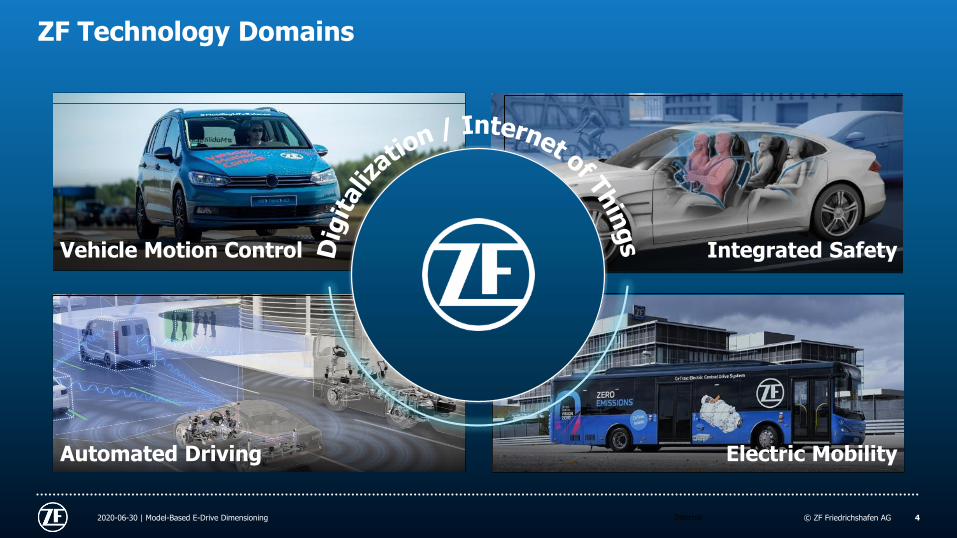
ZF Technology Domains
42020-06-30 | Model-Based E-Drive Dimensioning
Vehicle Motion Control
Automated Driving Electric Mobility
Integrated Safety

© ZF Friedrichshafen AGInternal2020-06-30 | Model-Based E-Drive Dimensioning 5
ZF Systems Expertise
Advanced Driver Assistance Systems
Electric Drives
Chassis Components
Steering Systems
Damping Systems
Safety Electronics
Active Chassis Systems
Axle Drives / Electric Axle Drives
Axle Systems
Braking Systems
Transmission Systems
Electronic Systems
Occupant Safety Systems
Electrified Powertrain: Vehicle Motion Control: Automated Driving: Integrated Safety:

Internal
ZF electrifies everything on wheelsFrom bikes and cars to trucks and buses
© ZF Friedrichshafen AGInternal © ZF Friedrichshafen AG© ZF Friedrichshafen AG
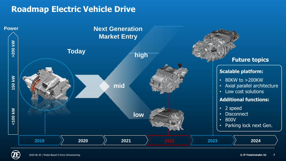
Roadmap Electric Vehicle Drive
72020-06-30 | Model-Based E-Drive Dimensioning
2019 2020 2021 2022 2023 2024
Today
>2
00
kW
<1
00
kW
Power
15
0 k
W
Next Generation
Market Entry
low
mid
high
Scalable platform:
• 80KW to >200KW• Axial parallel architecture• Low cost solutions
Additional functions:
• 2 speed• Disconnect• 800V• Parking lock next Gen.
Future topics
© ZF Friedrichshafen AGInternal © ZF Friedrichshafen AG2020-06-30 | Model-Based E-Drive Dimensioning 8
02E-Drive Concept
© ZF Friedrichshafen AGInternal 92020-06-30 | Model-Based E-Drive Dimensioning
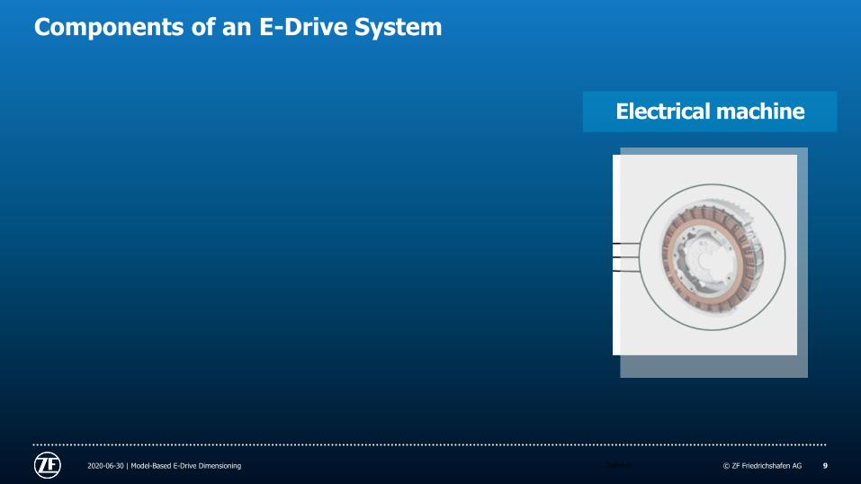
Components of an E-Drive System
Electrical machine

© ZF Friedrichshafen AGInternal 102020-06-30 | Model-Based E-Drive Dimensioning
Components of an E-Drive System
Energy source Electrical machine
© ZF Friedrichshafen AGInternal 112020-06-30 | Model-Based E-Drive Dimensioning
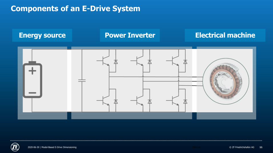
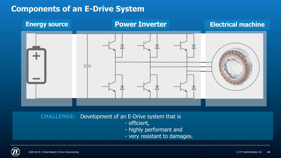
Components of an E-Drive System
Electrical machineEnergy source Power Inverter
© ZF Friedrichshafen AGInternal 122020-06-30 | Model-Based E-Drive Dimensioning
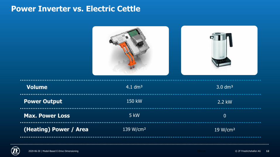
Power Inverter vs. Electric Cettle
Volume
Power Output
Max. Power Loss
(Heating) Power / Area
4.1 dm³
150 kW 2.2 kW
5 kW 0
139 W/cm² 19 W/cm²
3.0 dm³

© ZF Friedrichshafen AGInternal 132020-06-30 | Model-Based E-Drive Dimensioning
Power Inverter in action - „139W/cm²“
© ZF Friedrichshafen AGInternal 142020-06-30 | Model-Based E-Drive Dimensioning
Components of an E-Drive System
Electrical machineEnergy source
CHALLENGE: Development of an E-Drive system that is - efficient, - highly performant and- very resistant to damages.
Power Inverter
© ZF Friedrichshafen AGInternal
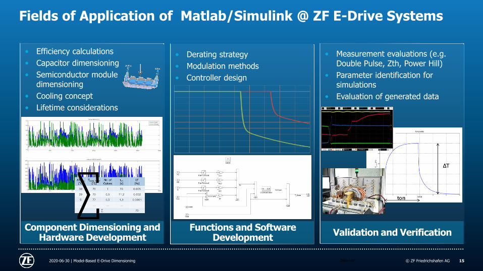
Fields of Application of Matlab/Simulink @ ZF E-Drive Systems
2020-06-30 | Model-Based E-Drive Dimensioning 15
• Efficiency calculations
• Capacitor dimensioning
• Semiconductor module dimensioning
• Cooling concept
• Lifetime considerations
Component Dimensioning and Hardware Development
• Measurement evaluations (e.g. Double Pulse, Zth, Power Hill)
• Parameter identification for simulations
• Evaluation of generated data
Validation and Verification
• Derating strategy
• Modulation methods
• Controller design
Functions and Software Development
© ZF Friedrichshafen AGInternal © ZF Friedrichshafen AG2020-06-30 | Model-Based E-Drive Dimensioning 16
03Matlab Inverter Model

© ZF Friedrichshafen AGInternal
System Parameters
…
Lifetime Model
172020-06-30 | Model-Based E-Drive Dimensioning
Efficiency
Diagrams
Performance
Diagrams
Lifetime
Calculations
Derating
Strategy
Matlab Inverter Model
Matlab Inverter Model
Thermal Losses
HeatGeneration
LifetimeConsump
-tion
Max. ElectricalCurrents
Loss Parameters
Operating Data Thermal
Parameters

© ZF Friedrichshafen AGInternal 182020-06-30 | Model-Based E-Drive Dimensioning
Invert
er
Model
Loss Modell
Standard Operation Mode
Highside
IGBTsSwitching Losses
Conduction Losses
DiodesSwitching Losses
Conduction Losses
Lowside
IGBTsSwitching Losses
Conduction Losses
DiodesSwitching Losses
Conduction Losses
Active Short Circuit
Highside
IGBTs
Switching Losses
Conduction Losses
DiodesSwitching Losses
Conduction Losses
Lowside
IGBTs Switching Losses
Conduction Losses
Diodes Switching Losses
Conduction Losses
Thermal Model
Coolant
IGBTs Highside
Diodes Highside
IGBTs Lowside
Diodes Lowside
Structure Inverter Model
Lines of Matlab Code
∑ Simulink Blocks
~10,000
>>3,000
ca. 10 years of development

© ZF Friedrichshafen AGInternal © ZF Friedrichshafen AG2020-06-30 | Model-Based E-Drive Dimensioning 19
04Applications
© ZF Friedrichshafen AGInternal © ZF Friedrichshafen AG2020-06-30 | Model-Based E-Drive Dimensioning 20
Efficiency and Performance Calculations
04-1

© ZF Friedrichshafen AGInternal
CO2 reduction: Every gram counts
212020-06-30 | Model-Based E-Drive Dimensioning
Conventional drivelines Electric drivelinesHybrid drivelines
CO2 reduction: Every gram counts
© ZF Friedrichshafen AGInternal 222020-06-30 | Model-Based E-Drive Dimensioning
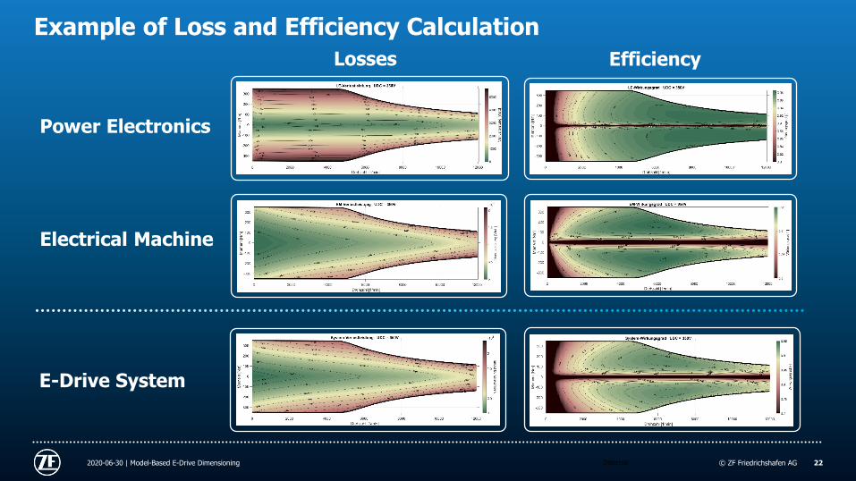
Example of Loss and Efficiency Calculation
Losses Efficiency
Power Electronics
Electrical Machine
E-Drive System

© ZF Friedrichshafen AGInternal 232020-06-30 | Model-Based E-Drive Dimensioning
Example of Loss and Efficiency CalculationLosses Efficiency
Power Electronics
Electrical Machine
E-Drive System
→ Losses and efficiency of entire E-Drive system calculated over torque and speed range
© ZF Friedrichshafen AGInternal 242020-06-30 | Model-Based E-Drive Dimensioning
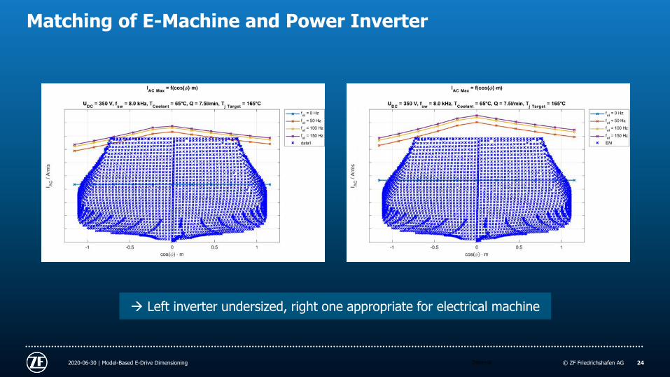
Matching of E-Machine and Power Inverter
→ Left inverter undersized, right one appropriate for electrical machine

© ZF Friedrichshafen AGInternal © ZF Friedrichshafen AG2020-06-30 | Model-Based E-Drive Dimensioning 25
04-2Lifetime Prediction

© ZF Friedrichshafen AGInternal 262020-06-30 | Model-Based E-Drive Dimensioning
• Different extension coefficients result in thermal stress.
• Each junction can absorb a certain amount of energy and will fail afterwards.
Ploss
∆T PLoss = f(Iac, fsw, Udc, TKM, ..)
• To predict time to failure of each junction, thermal stress has to be described mathematically.
Lifetime Simulation Semiconductor
Image source:G. Farks, D. Schweitzer, Z. Sarkany, M. RenczOn the Reproducibility of Thermal Measurements and of Related ThermalMetrics in Static and Transient Tests of Power Devices

© ZF Friedrichshafen AGInternal 272020-06-30 | Model-Based E-Drive Dimensioning
„Mission Profile“of Electr. Drive
(M, v, UBatt)
„Mission Profile“of Power Electronics
(UDC, I, cosφ, m, fel)
Simulation
Model EM
Temperature ProfileSemiconductor(TIGBT, TDiode)
Simulation
Model PE
Load Cycle of Semiconductor(∆T-Histogram)
Rainflow
Classification
Lifetime Consumptionof Semiconductors
Palmgren
Miner
Probability of Failureof Semiconductors
Weibull
Distribution
Input ofPower Cycling Test Results
Lifetime Consumptionper Temperature Rise
Power Cycling Stability
Coolant Temperature + Coolant Flow Rate
Workflow Lifetime Predicition

© ZF Friedrichshafen AGInternal 282020-06-30 | Model-Based E-Drive Dimensioning
-40 -30 -20 -15 -10 -5 0 5 10 15 20 25 30 35 40 45 50 55 60 65 70
Drive Cycle 1 1,255% 2,409% 4,481% 6,046% 8,104% 10,021% 12,313% 13,961% 16,357% 19,063% 22,560% 26,583% 22,326% 22,372% 22,964% 28,918% 36,264% 45,296% 56,361% 69,869% 86,308%
Drive Cycle 2 1,051% 2,013% 3,734% 5,032% 6,734% 8,382% 10,373% 11,960% 14,125% 16,591% 19,713% 23,320% 19,845% 20,034% 20,600% 25,923% 32,485% 40,546% 50,412% 62,444% 77,073%
Drive Cycle 3 0,716% 1,365% 2,522% 3,391% 4,528% 5,658% 7,031% 8,204% 9,753% 11,539% 13,770% 16,365% 14,232% 14,544% 15,034% 18,883% 23,618% 29,419% 36,504% 45,124% 55,578%
Drive Cycle 4 1,043% 1,994% 3,691% 4,967% 6,640% 8,268% 10,237% 11,835% 13,999% 16,474% 19,598% 23,216% 19,935% 20,229% 20,848% 26,205% 32,800% 40,889% 50,776% 62,818% 77,437%
Drive Cycle 5 0,765% 1,461% 2,703% 3,636% 4,858% 6,060% 7,518% 8,734% 10,358% 12,223% 14,563% 17,278% 14,925% 15,185% 15,653% 19,667% 24,607% 30,662% 38,060% 47,065% 57,991%
Drive Cycle 6 0,819% 1,563% 2,891% 3,888% 5,195% 6,475% 8,023% 9,294% 11,001% 12,954% 15,412% 18,256% 15,674% 15,888% 16,360% 20,556% 25,720% 32,051% 39,786% 49,201% 60,626%
Drive Cycle 7 0,398% 0,760% 1,406% 1,893% 2,530% 3,170% 3,950% 4,631% 5,526% 6,561% 7,856% 9,365% 8,241% 8,489% 8,827% 11,098% 13,894% 17,324% 21,518% 26,627% 32,830%
Distr. Cold 0,10% 0,20% 0,30% 0,70% 2,00% 3,00% 5,00% 15,00% 26,10% 25,70% 13,30% 5,00% 2,00% 1,00% 0,50% 0,10% 0,00% 0,00% 0,00% 0,00% 0,00%
Distr. Hot 0,00% 0,00% 0,00% 0,00% 0,00% 0,00% 0,00% 0,00% 0,00% 0,10% 0,50% 0,50% 1,30% 2,20% 4,70% 14,00% 27,10% 25,80% 14,70% 6,70% 1,60%
Cooling temperature in °C
Example of Lifetime Prediction
0%
20%
40%
60%
80%
100%
120%
140%
-40 -20 -10 0 10 20 30 40 50 60 70 80
Drive Cycle 1
Drive Cycle 2
Drive Cycle 3
Drive Cycle 4
Drive Cycle 5
Drive Cycle 6
Drive Cycle 7
Upper Bound
Cooling temperature in °C
Lifetim
e c
onsu
mption

© ZF Friedrichshafen AGInternal © ZF Friedrichshafen AG2020-06-30 | Model-Based E-Drive Dimensioning 29
05Conclusion & Outlook

© ZF Friedrichshafen AGInternal
Conclusion
• Challenge: E-Drive system → efficient, highly performant and persistent
• Development of Matlab/Simulink environment: enables evaluation of efficiency, performance, lifetime
• Entire E-drive system can be correctly dimensioned, improved and optimized by simulation!
Outlook
• Increase of level of automation
• Combining Matlab/Simulink environment with CAD-, FEM- and CFD-simulation environments
• Integration of EMC simulation in our simulation environment
302020-06-30 | Model-Based E-Drive Dimensioning
Conclusion & Outlook
© ZF Friedrichshafen AGInternal 312020-06-30 | Model-Based E-Drive Dimensioning
Questions & Answers
Contact: [email protected]


![Performance Evaluation of Integrated Voice/Data Services ... · radio resource dimensioning. For voice traffic over GSM, Erlang model [1] is still the main tool for resource dimensioning.](https://static.cupdf.com/doc/110x72/5b42ef767f8b9a85708b76cb/performance-evaluation-of-integrated-voicedata-services-radio-resource.jpg)