Mid-level Visual Element Discovery as Discriminative Mode Seeking
Harley Montgomery11/15/13

Main Idea
• What are discriminative features exactly, and how can we find them automatically?
• Discriminative features are local maxima in the feature distribution of positive/negative examples, p+(x)/p-(x)
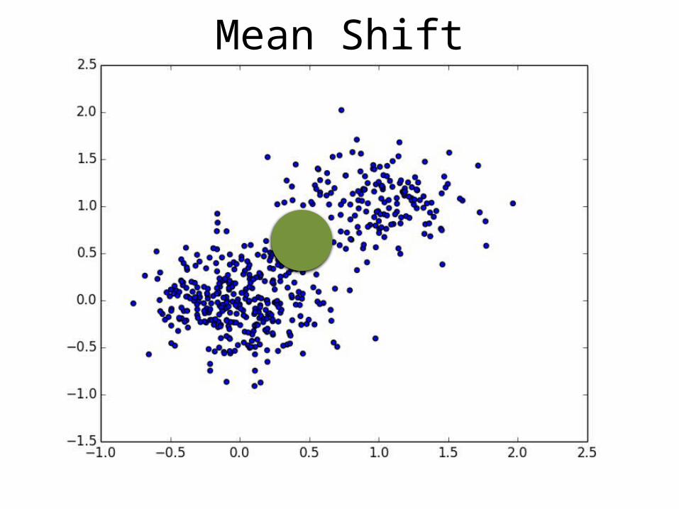
Mean Shift
Mean Shift
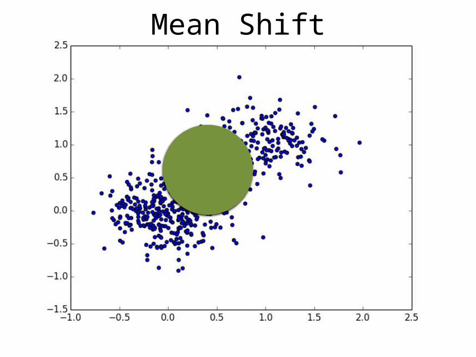
Mean Shift – 1st Issue
• HOG distances vary significantly across feature space, different bandwidths are needed in different regions
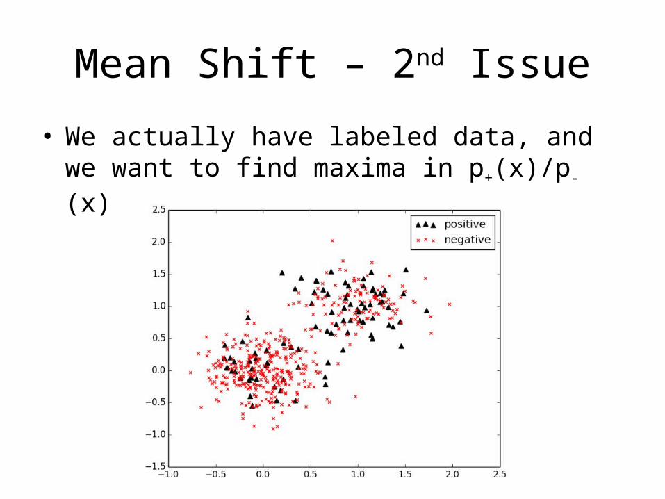
Mean Shift – 2nd Issue
• We actually have labeled data, and we want to find maxima in p+(x)/p-(x)
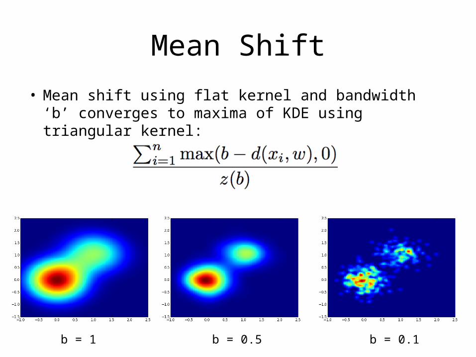
Mean Shift
• Mean shift using flat kernel and bandwidth ‘b’ converges to maxima of KDE using triangular kernel:
b = 1 b = 0.1b = 0.5
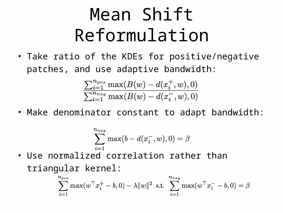
Mean Shift Reformulation
• Take ratio of the KDEs for positive/negative patches, and use adaptive bandwidth:
• Make denominator constant to adapt bandwidth:
• Use normalized correlation rather than triangular kernel:
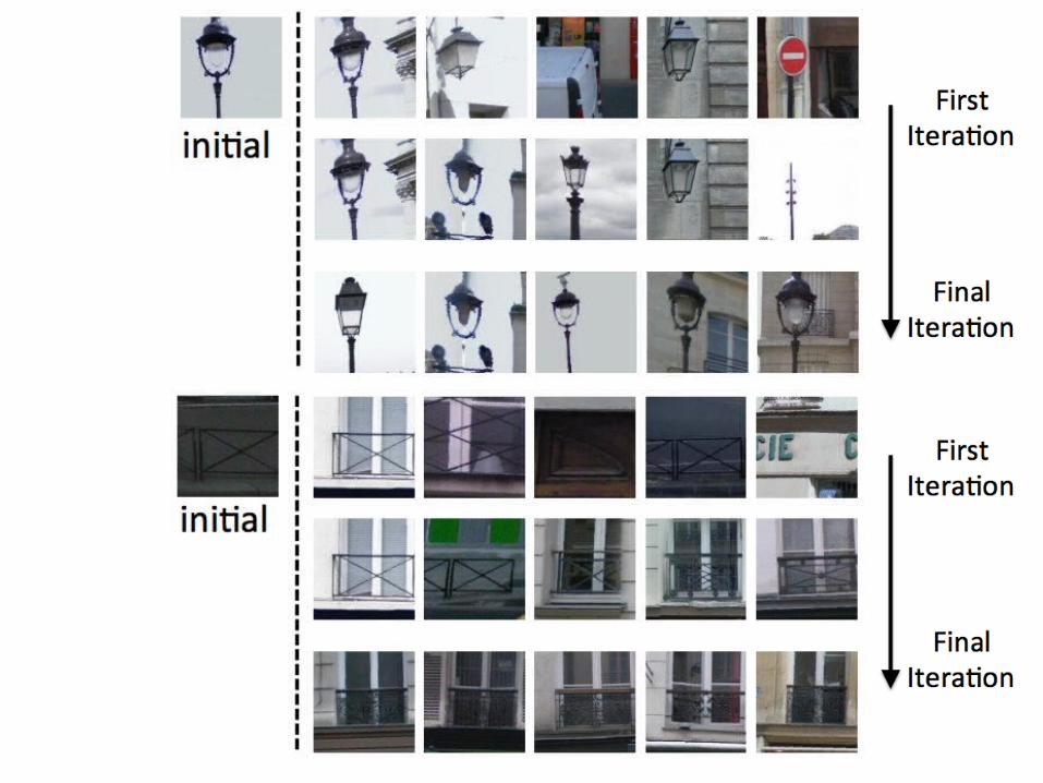
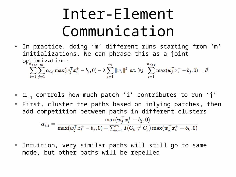
Inter-Element Communication• In practice, doing ‘m’ different runs starting from ‘m’ initializations. We
can phrase this as a joint optimization:
• αi,j controls how much patch ‘i’ contributes to run ‘j’• First, cluster the paths based on inlying patches, then add competition
between paths in different clusters
• Intuition, very similar paths will still go to same mode, but other paths will be repelled
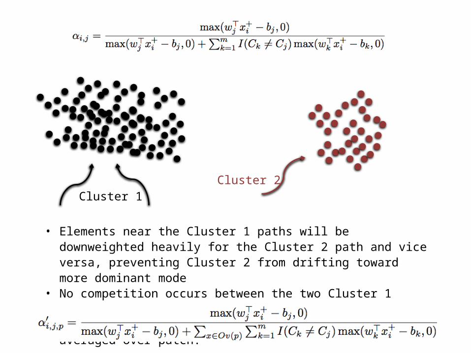
Cluster 1Cluster 2
• Elements near the Cluster 1 paths will be downweighted heavily for the Cluster 2 path and vice versa, preventing Cluster 2 from drifting toward more dominant mode
• No competition occurs between the two Cluster 1 paths• In practice, calculated a per pixel quantity and averaged over patch:

No inter-element communication
With inter-element communication
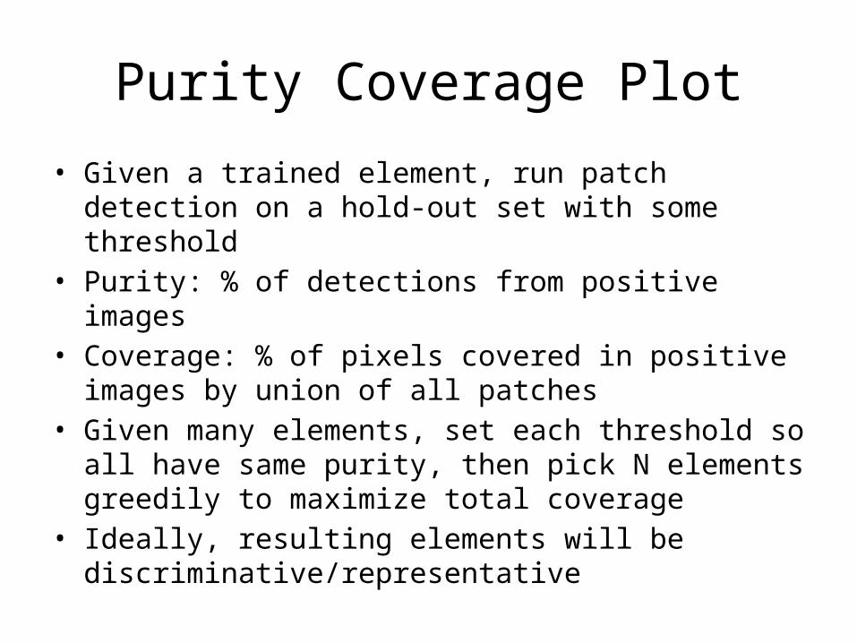
Purity Coverage Plot
• Given a trained element, run patch detection on a hold-out set with some threshold
• Purity: % of detections from positive images• Coverage: % of pixels covered in positive images by union of
all patches• Given many elements, set each threshold so all have same
purity, then pick N elements greedily to maximize total coverage
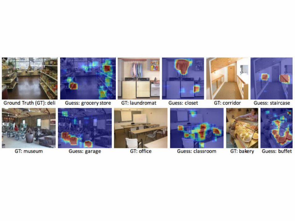
• Ideally, resulting elements will be discriminative/representative

• Discriminative mode seeking finds better elements than previous methods
Purity Coverage Plot
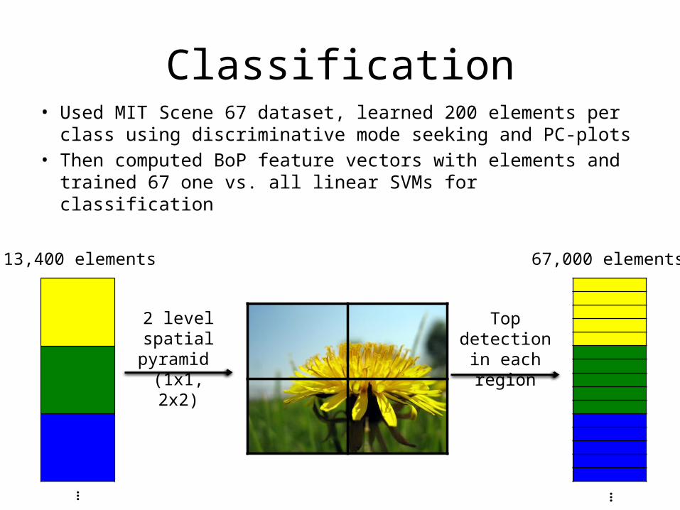
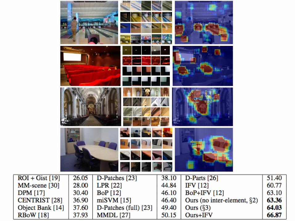
Classification• Used MIT Scene 67 dataset, learned 200 elements per class
using discriminative mode seeking and PC-plots• Then computed BoP feature vectors with elements and
trained 67 one vs. all linear SVMs for classification
13,400 elements
2 level spatial pyramid (1x1, 2x2)
Top detection in each region
67,000 elements
… …

Conclusion
• Defined discriminative elements as maxima in the ratio between positive/negative distributions
• Adapted mean shift algorithm to find the maxima in these distributions
• Introduced PC plots to choose best elements out of many
• Achieved state-of-the-art accuracy on MIT Scene 67 dataset